8 Quantum Cluster Methods

Erik KochComputational Materials ScienceGerman Research School for Simulation SciencesJulich

Contents1 Periodic systems 4

1.1 Lattices . . . . . . . . . . . . . . . . . . . . . . . . . . . . . . . . . . . . . . 41.2 Superlattices . . . . . . . . . . . . . . . . . . . . . . . . . . . . . . . . . . . . 8

2 Variational methods 102.1 Variational Monte Carlo . . . . . . . . . . . . . . . . . . . . . . . . . . . . . 142.2 Correlated sampling . . . . . . . . . . . . . . . . . . . . . . . . . . . . . . . . 162.3 Gutzwiller approximation . . . . . . . . . . . . . . . . . . . . . . . . . . . . . 182.4 Brinkman-Rice transition . . . . . . . . . . . . . . . . . . . . . . . . . . . . . 20

3 Projection techniques 233.1 Importance sampling . . . . . . . . . . . . . . . . . . . . . . . . . . . . . . . 243.2 Fixed-node Monte Carlo . . . . . . . . . . . . . . . . . . . . . . . . . . . . . 253.3 Optimization of the trial function . . . . . . . . . . . . . . . . . . . . . . . . . 263.4 Quasi-particle energies . . . . . . . . . . . . . . . . . . . . . . . . . . . . . . 30

4 Conclusion 35

E. Pavarini, E. Koch, D. Vollhardt, and A. LichtensteinDMFT at 25: Infinite DimensionsModeling and Simulation Vol. 4Forschungszentrum Julich, 2014, ISBN 978-3-89336-953-9http://www.cond-mat.de/events/correl14

8.2 Erik Koch

The central challenge of electronic structure theory is the solution of the many-electron Hamil-tonian in the Born-Oppenheimer approximation (in atomic units)

H = −1

2

∑i

~∇2i +

∑i

Vext(~ri) +∑i<j

1

|~ri − ~rj|, (1)

where the external potential is, e.g., the Coulomb potential of the nuclei of charge ZI at position~RI , shifted by their mutual Coulomb interaction

Vext(~r) =∑I

ZI

|~r − ~RI |+∑I<J

ZIZJ

|~RI − ~RJ |. (2)

Introducing a basis-set {ϕα(x)} of spin-orbitals, we can rewrite H in second quantization

H = −∑αβ

tαβ c†αcβ +

1

2

∑αβγδ

Uαδβγc†αc†βcγcδ (3)

where the creation/annihilation operators fulfill the anticommutation relations {c†α, c†β} = 0 =

{cα, cβ} and {cα, c†β} = 〈α|β〉 = Sαβ , and S is the overlap matrix [1]. The matrix elements are

given by integrating over the orbital degrees of freedom x = (~r, σ)

tαβ =∑α′β′

(S−1)αα′

∫dx ϕα′(x)

(1

2~∇2 − Vext(~r )

)ϕβ′(x) (S−1)β′β (4)

and

Uαδβγ

=∑α′δ′β′γ′

S−1αα′ S

−1ββ′

∫dx

∫dx′ ϕα′(x)ϕβ′(x′)

1

|~r − ~r ′|ϕγ′(x

′)ϕδ′(x) S−1γ′γ S

−1δ′δ . (5)

This representation of the Hamiltonian is suited for introducing approximations. By truncatingthe basis-set to only K functions, the Hilbert space H of H for a system with N electrons isrestricted to a finite variational subspaceH({ϕαn(x); |n = 1 . . . K}) of dimension

(KN

). Work-

ing with a finite basis set introduces a basis-set error. To keep it small, the basis functions arechosen such that the eigenstates of interest are represented well onH({ϕαn(x) |n = 1 . . . K}),using, e.g., low-energy orbitals to represent the ground state. The basis-set error can be esti-mated by comparing results calculated with basis sets of increasing size and extrapolating to thecomplete-basis-set-limit. Such calculations are computationally demanding, as the dimensionof the Hilbert space increases for K � N � 1 (using Stirling’s approximation) with a highpower, given by the (fixed) number of electrons in the system, as O(KN).For extended systems the problem becomes even harder. To ensure size-consistency [2], mean-ing that the basis-set error for extensive observables, e.g., the total energy, scales at most withthe number of electrons, we have to increase K along with N , leading to an exponential scal-ing of the variational space with system size. Practical simulations are therefore restricted toquite small clusters. These have a large fraction of surface atoms. As a simple example, fora 10 × 10 × 10 cluster 488 of the 1000 atoms are on the surface. The surface effects can be

Quantum Cluster Methods 8.3

removed by putting the system in a simulation cell spanned by three vectors ~Ri and assumingthat the system is periodically repeated [3]. Instead of leaving the system, an electron passingthrough a face of the simulation cell continues into the neighboring cell, while one of its im-ages enters through the opposite face. Thus, we are dealing with an extended system with aninfinite number of electrons. Still, by virtue of the periodicity, only the N electrons inside thesimulation cell are independent degrees of freedom. We can then restrict the calculation to thesimulation cell C =

{∑i xi

~Ri

∣∣ xi ∈ [0, 1)}

by including the periodic images of the externalpotential (created inside the simulation cell) and the interaction with the electrons outside thesimulation box in the Hamiltonian [4]

Hpbc = −1

2

N∑i=1

~∇2i +

∑~n∈Z3

∑i

V Cext(~ri − ~R~n) +1

2

∑~n∈Z3

∑i,j

′ 1

|~ri − ~rj − ~R~n|. (6)

where ~R~n =∑3

i=1 ni~Ri and the prime on the last sum indicates that i 6= j when ~n = 0. The

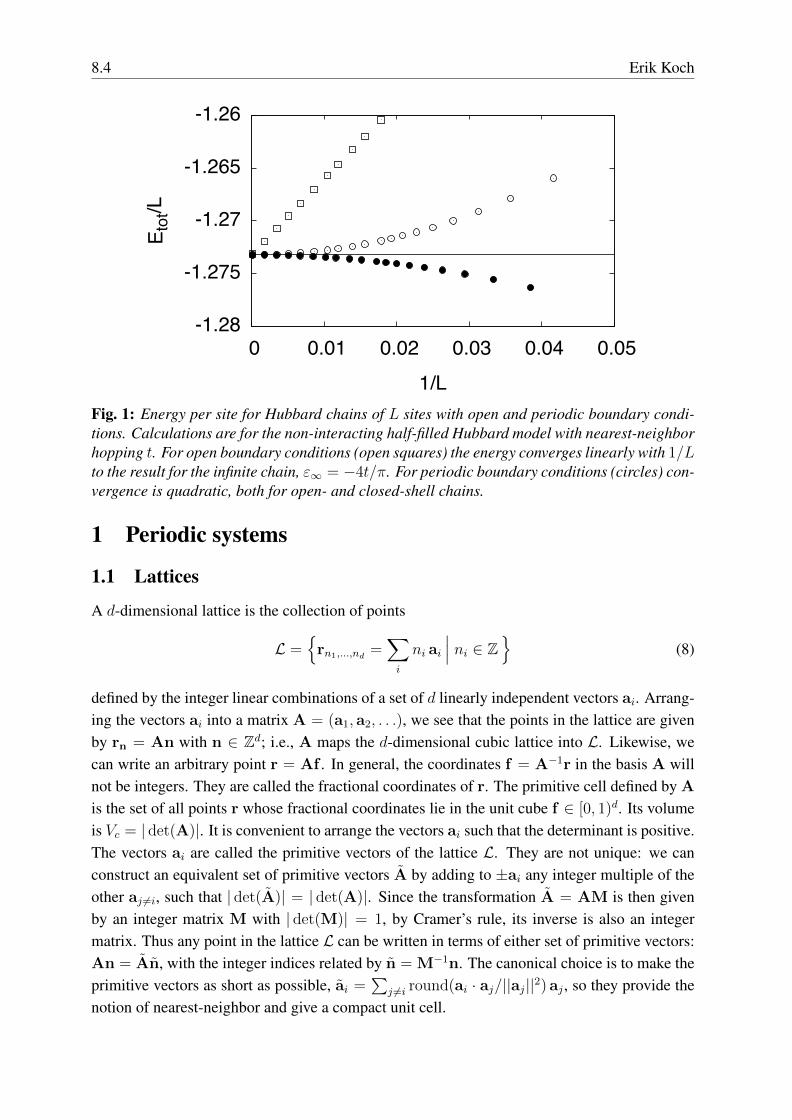
eigenfunctions of (6) on the simulation cell C represent a system of average electron densityN/VC . We see that, while removing surface effects, the introduction of periodic boundary con-ditions not only modifies interactions of ranges longer than the radius of the simulation cellbut also suppress fluctuations of the number of electrons between simulation cells. Moreover,the average electron density can only be a multiple of 1/VC as the simulation cell must con-tain an integer number of electrons. Obviously, these finite-size errors vanish in the limit ofinfinite simulation cell volume VC → ∞. Fig. 1 shows a comparison of the finite-size scalingfor the ground-state energy with open and with periodic boundary conditions. For systems thatdevelop long-range correlations, care has to be taken in the finite-size extrapolation for corre-lation functions C(~r, ~r′), as imposing periodic boundary conditions C(~r, ~r + ~Ri) = C(~r, ~r′)

can frustrate correlations that are not commensurate with the simulation cell. This becomesparticularly evident for a crystal in which the external potential of the infinite system is periodicVext(~r + ~ai) = Vext(~r ) with the periodicity of the lattice spanned by the vectors ~ai. Only whenthe vectors ~Ri spanning C are chosen as integer linear combinations ~Ri =

∑j nij ~aj will the

external potential in Hpbc agree with Vext:∑~n∈Z3

V Cext(~r − ~R~n) = Vext(~r) , (7)

where V Cext is the external potential originating, e.g., from the nuclei inside C.For such periodic systems the nature of the many-body problem becomes apparent. The inter-action term by itself is not particularly complicated. It is diagonal in real space, so finding thearrangement of electrons that minimizes their mutual Coulomb repulsion is a straightforwardclassical optimization problem, the solution being a Wigner crystal [5]. The kinetic energy,on the other hand, is diagonal in k-space. For a lattice-periodic potential, Vext couples only adiscrete set of k-vectors, so that the single-electron part of H can be solved in terms of Blochwaves. Solutions of the full problem thus have to balance the extended Bloch waves (kineticenergy) against the localized Wigner crystal (electron-electron repulsion).

8.4 Erik Koch

-1.28

-1.275

-1.27

-1.265

-1.26

0 0.01 0.02 0.03 0.04 0.05

E tot

/L

1/LFig. 1: Energy per site for Hubbard chains of L sites with open and periodic boundary condi-tions. Calculations are for the non-interacting half-filled Hubbard model with nearest-neighborhopping t. For open boundary conditions (open squares) the energy converges linearly with 1/Lto the result for the infinite chain, ε∞ = −4t/π. For periodic boundary conditions (circles) con-vergence is quadratic, both for open- and closed-shell chains.

1 Periodic systems

1.1 Lattices

A d-dimensional lattice is the collection of points

L ={

rn1,...,nd =∑i

ni ai

∣∣∣ ni ∈ Z}

(8)

defined by the integer linear combinations of a set of d linearly independent vectors ai. Arrang-ing the vectors ai into a matrix A = (a1, a2, . . .), we see that the points in the lattice are givenby rn = An with n ∈ Zd; i.e., A maps the d-dimensional cubic lattice into L. Likewise, wecan write an arbitrary point r = Af . In general, the coordinates f = A−1r in the basis A willnot be integers. They are called the fractional coordinates of r. The primitive cell defined by A

is the set of all points r whose fractional coordinates lie in the unit cube f ∈ [0, 1)d. Its volumeis Vc = | det(A)|. It is convenient to arrange the vectors ai such that the determinant is positive.The vectors ai are called the primitive vectors of the lattice L. They are not unique: we canconstruct an equivalent set of primitive vectors A by adding to ±ai any integer multiple of theother aj 6=i, such that | det(A)| = | det(A)|. Since the transformation A = AM is then givenby an integer matrix M with | det(M)| = 1, by Cramer’s rule, its inverse is also an integermatrix. Thus any point in the lattice L can be written in terms of either set of primitive vectors:An = An, with the integer indices related by n = M−1n. The canonical choice is to make theprimitive vectors as short as possible, ai =

∑j 6=i round(ai · aj/||aj||2) aj , so they provide the

notion of nearest-neighbor and give a compact unit cell.

Quantum Cluster Methods 8.5

The reciprocal latticeRL associated with L arises naturally when considering the Fourier trans-form of lattice periodic functions, i.e., functions V (r + An) = V (r). The Fourier expansion ofa general function V (r) is given by

V (r) =

∫ddk V (k) eik·r . (9)

When V (r) is periodic on L, we have

V (r + An) =

∫ddk V (k) eik·r eik·An = V (r) . (10)

By the linear independence of Fourier modes it follows that only terms with exp(ik ·An) = 1

for all n ∈ Zd can contribute. The k-vectors fulfilling this condition form the reciprocal lattice

RL ={

Gm∣∣ m ∈ Zd

}(11)

with primitive vectors G = (2πA−1)T . Since (2πG−1)T = A, the reciprocal lattice of RLis L. By construction, the reciprocal lattice vectors g ∈ RL define plane waves exp(ig · r)

for which all lattice points rn ∈ L fall on planes of phase = 1. The reciprocal lattice vectors,except the gamma-point g = 0, are thus orthogonal to planes containing an infinite number oflattice points. A given set of lattice planes can be characterized by the shortest reciprocal latticevector gmin = Gm perpendicular to it. The expansion coefficients m in terms of the primitivereciprocal vectors are the Miller indices. As for the real lattice, the primitive vectors are notunique: A = AM gives G = (2πA−1)T = G(M−1)T , which also span RL. The canonicalchoice for the primitive reciprocal cell is k ∈ G (−1/2, 1/2]d. A momentum k from a primitivereciprocal cell (first Brillouin zone) is called a crystal momentum.Transforming the single-electron Hamiltonian

Hsingle = −1

2∇2

r + Vext(r) (12)

with lattice-periodic potential Vext(r) =∑

m∈Zd VGm eiGm·r to k-space

〈k|Hsingle|k′〉 =k2

2δ(k− k′) + VGm δ(k− k′ −Gm) (13)

or, more elegantly,

Hsingle =∑k

k2

2c†k,σ ck,σ +

∑k

∑m∈Zd

VGm c†k+Gm,σ ck,σ , (14)

we see that the Hamiltonian only couples states whose wave-vectors differ by reciprocal latticevectors (for m 6= 0 they are Umklapp processes). Thus, Hsingle is block-diagonal in k-space sothat its eigenstates are of the form

ϕn,k(r) =∑m∈Zd

cn,m ei(k+Gm)·r , (15)

8.6 Erik Koch

where k, now restricted to the primitive reciprocal cell, is the cryrstal momentum of the stateand n its band index. Under translations by a lattice vector An they transform as

ϕn,k(r + An) = eik·An ϕn,k(r) , (16)

i.e., as irreducible representations of the abelian translation group. This is the Bloch theorem.Transforming back to real space, we could determine the eigenfunctions ϕn,k(r) by solving theeigenvalue problem for Hsingle(

1

2∇2

r + Vext(r)

)ϕn,k(r) = εn,k ϕn,k(r) (17)

not on the entire space Rd, but on a single primitive lattice cell imposing k-boundary conditionsϕn,k(ai) = eik·ai ϕn,k(0). It is, however, more common to rewrite (15) as

ϕn,k(r) = eik·r∑m

cn,m eiGm·r = eik·r un,k(r) . (18)

with the lattice-periodic Bloch function un,k(r). Using this form as an ansatz in (17), we seethat the Bloch functions can be obtained from the eigenvalue problem(

1

2

(− i∇r + k

)2+ V (r)

)un,k(r) = εn,k un,k(r) , (19)

on a primitive cell of Lwith periodic boundary conditions. We note that in this equation k playsthe role of a constant vector potential.For a general time-reversal-symmetric Hamiltonian, every eigenfunction ϕα(r) is degeneratewith its complex conjugate, so that we can choose real eigenfunctions. Taking the complexconjugate of (19) shows that for a real potential we can choose un,k(r) = un,−k(r). When thepotential is inversion-symmetric, V (−r) = V (r), then ϕα(−r) is degenerate with ϕα(r). For(19) it implies un,k(−r) = un,−k(r). In the presence of both symmetries we obtain un,k(r) =

un,−k(r) = un,k(−r).A Bloch theorem also holds for the eigenstates of a many-body Hamiltonian that is invariantunder lattice translations. Translating all electrons by the same lattice vector An will multiplythe wave-function by a phase eiktot·An, where ktot is the total crystal momentum of the many-body state. Thus, in k-space the Hamiltonian block-diagonalizes into sectors with a given totalcrystal momentum. Writing H in k-space

H =∑k,σ

(k2

2c†k,σ ck,σ +

∑m

VGm c†k+Gm,σck,σ +1

2

∑k′,σ′;q

c†k+q,σc†k′−q,σ′

1

|q |2ck′,σ′ck,σ

)(20)

we see that acting on a Slater determinant of plane waves with momenta ki (or Bloch waves ofcrystal momenta ki), the Hamiltonian does not change total crystal momentum ktot =

∑ki.

However, while the kinetic energy is diagonal and the external potential scatters only betweenplane waves differing by a reciprocal lattice vector, the electron-electron interaction scatters

Quantum Cluster Methods 8.7

plane waves of arbitrary single-electron momentum. Thus, for the eigenvalue problem we haveto consider Slater determinants of plane waves with arbitrary wave-vectors ki.As the simplest example, let us consider the Slater determinant of two plane waves

Φk1,k2(r1, r2) =1√2

(1

(2π)d/2

)2∣∣∣∣∣ eik1·r1 eik2·r1

eik1·r2 eik2·r2

∣∣∣∣∣ ∝ ei(k1·r1+k2·r2) − ei(k2·r1+k1·r2) (21)

By construction it transforms as desired under a shift of all electrons by a lattice vector

Φk1,k2(r1 + An, r2 + An) = e(k1+k2)·An Φk1,k2(r1, r2) . (22)

The situation is, however, markedly different from the single-electron case (15): there, we canalways translate a single electron coordinate into a primitive cell, allowing us to consider thesingle-electron Bloch functions on a finite volume. For more electrons, however, their relativedistance is unchanged under the collective translation, so that we cannot bring all coordinatesinto a finite volume. To make this possible, we would need a Bloch-type theorem for translationsof individual electrons:

Φk1,k2(r1 + c, r2) = eik·c Φk1,k2(r1, r2) (23)

(the equivalent equation for translations of r2 follows from the antisymmetry). Inserting (21) wesee that such an individual-electron Bloch-condition puts constraints on the allowed momenta:exp(i(ki− k) ·c) = 1. Thus, to be able to restrict the many-electron wavefunction to a primitivecell spanned by three vectors C with boundary conditions

Φk1,k2(ci, r2, . . .) = eik·ci Φk1,k2(0, r2, . . .) , (24)

we can only allow Slater determinants constructed from plane waves with wave vectors ki suchthat the ki − k are reciprocal lattice vectors of C. For k = 0 we obtain the simulation cellwith periodic boundary conditions discussed in the introduction. The eigenfunctions of H withboundary conditions (24) can be written in the Bloch-like form

ΨCn,k

(r1, r2, . . .) = eik·∑i ri UC

n,k(r1, r2, . . .) , (25)

where UCn,k

(r1, r2, . . .) is invariant under translations of a single electron by a vector from C andantisymmetric under particle exchange. While UC

n,kapparently is the many-body generalization

of the single-electron Bloch function un,k(r), we have to keep in mind that its construction isbased on the artificial boundary conditions (24), which depend on the choice of the volume C.When the volume is chosen small, calculations are simple but the wave functions ΨC

n,kwill give

poor approximations to the actual ground state, while increasing the cell improves the accuracybut also makes calculations increasingly difficult.Physically, as in the single-electron case (19), the twisted boundary conditions (24) correspondto a constant vector potential. The dependence of the ground state energy EC

0 (k) can be usedto distinguish metallic from (Mott) insulating systems: the second derivative at k = 0 of theenergy with respect to the current driving vector potential gives the static response. For metalsit stays finite while for insulators it vanishes in the thermodynamic limit [6].

8.8 Erik Koch

1.2 Superlattices

For a system with lattice periodicity the single- and many-electron boundary conditions (16) and(24) should be consistent. This implies, in particular, that the vectors spanning the cell should beinteger linear-combinations of the primitive lattice vectors, ci =

∑ai lij , or, in matrix notation,

C = AL, where the columns of L are the primitive cell vectors in units of the primitive latticevectors. The vectors C span a lattice S ⊆ L, called a superlattice. The volume of the primitiveunit cell of C is | det(L)| times the volume of the primitive lattice cell. Since L is an integermatrix, its determinant is also an integer.As the choice of the primitive lattice vectors A for a given latticeL is not unique, so is the choiceof L for a given superlattice S. We can, however, easily check whether, for given primitivelattice vectors A, two integer matrices span the same superlattice by reducing them to theirHermite normal form [7] and checking if they agree. The reduction of a non-singular integermatrix L to its Hermite normal form (HNF)

Λ =

λ11 0 0 · · ·λ21 λ22 0

λ31 λ32 λ33

... . . .

(26)

with λii ≥ 1, and λii > λij ≥ 0 can be done recursively. Allowed operations that leave thesuperlattice spanned by the transformed matrix unchanged are (i) multiplying a column by ±1,(ii) exchanging columns, and (iii) adding an integer multiple of another column. The reductionalgorithm [8] is based on the Euclidean algorithm for finding the greatest common divisor

gcd(a, b) =

|a| if b = 0 (operation of type (i))gcd(b, a) if |a| < |b| (operation of type (ii))gcd(a− ba/bcb, b) otherwise (operation of type (iii))

(27)

where a and b are the matrix elements in a given row of the matrix, and we perform the op-erations not just on these matrix elements but on their entire column vectors. To reduce thefirst row of L to the required form, we apply the Euclidean algorithm on the last two columns,reducing the coefficient in the last column to zero. In this way we reduce all matrix elementsexcept the first to zero, obtaining λ11 = gcd(l11, . . . , l1d). We iterate this procedure for the sub-matrix obtained by removing the first row and column to bring the matrix to lower triangularform. Finally, we use column operations to replace the off-diagonal elements in a row by theirremainders on division by the corresponding diagonal element.Besides giving a criterion for determining equivalent primitive cell vectors, the Hermite normalform gives a prescription for enumerating all non-equivalent periodic clusters of a given size.We have to be careful, however, when the lattice L spanned by A has point symmetries besidessimple inversion. Since the construction of Λ contains no information on the underlying lattice,such additional symmetries can render superlattices with different HNF equivalent.Fig. 2 gives an example of how different equivalent primitive cells can appear. For the squarelattice with point-symmetry C4v, we see that primitive vectors spanning the same superlattice

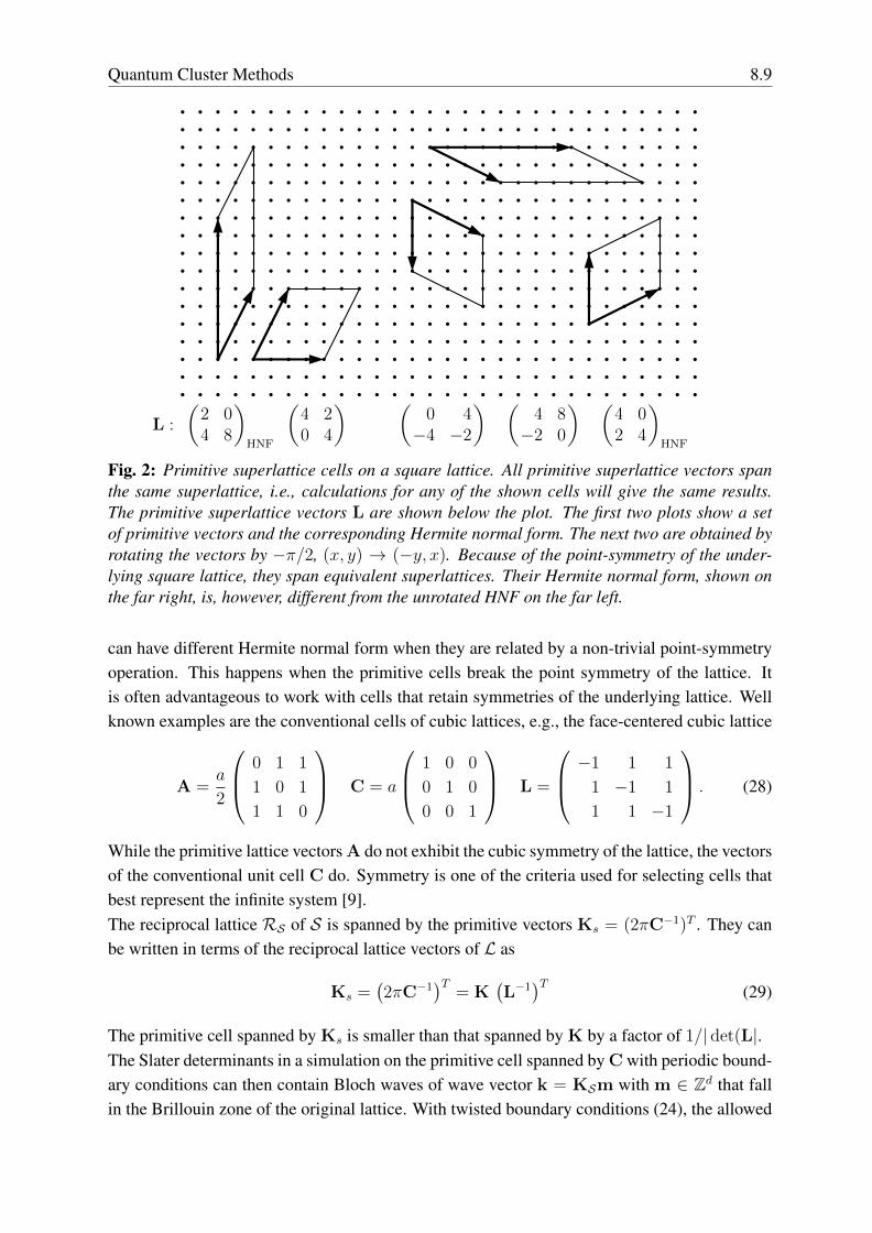
Quantum Cluster Methods 8.9

L :

(2 04 8

)HNF

(4 20 4

) (0 4−4 −2

) (4 8−2 0

) (4 02 4

)HNF

Fig. 2: Primitive superlattice cells on a square lattice. All primitive superlattice vectors spanthe same superlattice, i.e., calculations for any of the shown cells will give the same results.The primitive superlattice vectors L are shown below the plot. The first two plots show a setof primitive vectors and the corresponding Hermite normal form. The next two are obtained byrotating the vectors by −π/2, (x, y) → (−y, x). Because of the point-symmetry of the under-lying square lattice, they span equivalent superlattices. Their Hermite normal form, shown onthe far right, is, however, different from the unrotated HNF on the far left.

can have different Hermite normal form when they are related by a non-trivial point-symmetryoperation. This happens when the primitive cells break the point symmetry of the lattice. Itis often advantageous to work with cells that retain symmetries of the underlying lattice. Wellknown examples are the conventional cells of cubic lattices, e.g., the face-centered cubic lattice

A =a

2

0 1 1

1 0 1

1 1 0

C = a

1 0 0

0 1 0

0 0 1

L =

−1 1 1

1 −1 1

1 1 −1

. (28)

While the primitive lattice vectors A do not exhibit the cubic symmetry of the lattice, the vectorsof the conventional unit cell C do. Symmetry is one of the criteria used for selecting cells thatbest represent the infinite system [9].The reciprocal lattice RS of S is spanned by the primitive vectors Ks = (2πC−1)T . They canbe written in terms of the reciprocal lattice vectors of L as

Ks =(2πC−1

)T= K

(L−1

)T (29)

The primitive cell spanned by Ks is smaller than that spanned by K by a factor of 1/| det(L|.The Slater determinants in a simulation on the primitive cell spanned by C with periodic bound-ary conditions can then contain Bloch waves of wave vector k = KSm with m ∈ Zd that fallin the Brillouin zone of the original lattice. With twisted boundary conditions (24), the allowed

8.10 Erik Koch

wave vectors are shifted by k. The choice k = ki/2 corresponds to a sign-change under atranslation by ci, i.e., antiperiodic boundary conditions in that direction.When the primitive superlattice vectors are chosen as integer multiples of the primitive latticevectors, ci = ni ai, the reciprocal lattice shifted by k =

∑i(ni − 1)ki/2ni forms a Monkhorst-

Pack grid of special k-points that are popular for Brillouin-zone integrations [10].

2 Variational methods

Conceptually, the variational approach is straightforward: to find the ground state of a Hamil-tonian H, just minimize the energy expectation value

E[Ψ ] =〈Ψ |H|Ψ〉〈Ψ |Ψ〉

. (30)

The practical problem is, of course, the choice of a suitable variational space. The system-atic approach is to write the trial wave function as a linear combination of Slater determi-nants Ψ(r) =

∑α cα Φα(r) and allow all amplitudes cα to vary. For a finite system with N

electrons and a finite basis set of K orbitals there will be(KN

)Slater determinants. Mini-

mizing E[Ψ ] = E(c1, c2, . . .) amounts then to a high-dimensional optimization problem. AsE(c1, c2, . . .) has no local minima, this can be done using a steepest descent method, e.g., theLanczos method [11]. It involves the repeated application of the Hamiltonian to the trial func-tion. When working with a basis set, a Hamiltonian (2) with pair interaction only couplesSlater determinants that differ in at most two orbitals. Thus, the matrix representation of H inSlater-determinant space is reasonably sparse so that the matrix-vector product can be efficientlycalculated. Nevertheless this method, called configuration interaction (CI) as it describes the in-terplay of Slater determinants (electron configurations), is limited to quite small systems by thesheer number of Slater determinants spanning the Hilbert space, or, equivalently, by the numberof parameters cα that need to be simultaneously optimized: For a system with 25 electrons andjust 50 basis functions, the number of parameter is already above 1014, i.e., requiring a peta byteof memory just for storing the parameters cα. A way out might be to consider only “important”Slater determinants. It turns out that the variational energy converges, however, only slowlywith the number of determinants included in the calculation. Moreover, when we want to studysystems of increasing size a truncated CI easily leads to size-consistency problems [2].An alternative to the full-CI ansatz are wave functions that capture the strongest effects of elec-tron correlation with only a small number of parameters. To identify the major effect of electroncorrelation on the wave function, we return to the energy expectation value (30). Considered asa wave function functional, the stationarity condition

0 =δE

δΨ=H|Ψ〉〈Ψ |Ψ〉

− 〈Ψ |H|Ψ〉〈Ψ |Ψ〉2

|Ψ〉 (31)

is equivalent to the Schrodinger equation H Ψ(r) = E Ψ(r). Dividing by the wave function weobtain the local energy

Eloc(r) =H Ψ(r)

Ψ(r), (32)

Quantum Cluster Methods 8.11

which is constant for eigenstates ofH , i.e., its variance is zero (zero variance property). We canthus find eigenstates by minimizing the variance of the local energy (variance minimization)

σ2[Ψ ] =

∫|Eloc(r)|2 |Ψ(r)|2 dr−

(∫Eloc(r) |Ψ(r)|2 dr

)2

= 〈Ψ |H2|Ψ〉 − 〈Ψ |H|Ψ〉2. (33)

This approach can also be employed for constructing good trial wave functions.We might think that, as the solution of a second-order differential equation, wave functionsare smooth with continuous first derivative. This is, however, not true at singularities in thepotential. A well-known example is the hydrogen atom. Its ground state fulfills

Hϕ1s(~r) = −1

2~∇2ϕ1s(~r)−

1

rϕ1s(~r) = E1s ϕ1s(~r) . (34)

For r → 0, the potential energy diverges while Hϕ1s(~r) remains finite. For this reason, the 1s

function goes to a finite value at the position of the nucleus, producing a cusp , i.e., a discon-tinuity in the first derivative, which gives rise to the canceling divergence in the kinetic energy.The cancelation condition determining the cusp in the wave function, in the case of hydrogenϕ1s ∼ exp(−

√x2 + y2 + z2), is called the cusp condition [12]. Removing divergences in the

local energy by implementing the cusp condition is the most important step towards reducingthe variance of Eloc(r), i.e., constructing good variational wave functions.The cusps at the position of the nuclei are built into the single-particle orbitals obtained froma mean-field solution of (1). The many-body eigenstates will, however, also have cusps whentwo electrons meet (~ri → ~rj). These cusps are, of course, not easily reproduced by a linearcombination of Slater determinants, which explains the slow convergence of CI expansions.To derive the cusp conditions, we start with the electron-nucleus cusp. Following the exampleof hydrogen, we write the wave function close to a nucleus of charge Z as exp(−uZ(r)), wherer is the distance of the electron from the nucleus. For r close to zero the local energy is

Eloc(r) = −1

2

(d2

dr2+ 2

rddr

)e−uZ(r)

e−uZ(r)− Z

r= −−u′′Z(r) + u′Z

2(r)− 2u′Z(r)

r

2− Z

r. (35)

Thus, it stays finite for r → 0 when

duZdr

∣∣∣∣r=0

= +Z . (36)

For electrons, the cusp condition will depend on their relative spin orientation. Electrons withopposite spin need not be antisymmetrized so that we can write the wave function when theelectrons are close to each other as exp(−uσ,−σ(r)) with r = |r1 − r2|. The situation is almostthe same as for the electron-nucleon cusp, except that (i) electrons repel each other and (ii) wenow have two electronic degrees of freedom, i.e., we get contributions from the kinetic energyoperator for both electrons, resulting in

duσ,−σdr

∣∣∣∣r=0

= −1

2. (37)

8.12 Erik Koch

For electrons with parallel spin, the wave function must be antisymmetric in the electron co-ordinates, i.e., there must be a nodal surface separating the region where the wave function ispositive from that where it is negative. For r1 ≈ r2 we can approximate the nodal surface bya · r = 0, which is a plane when we keep one of the electron coordinates fixed. We can thenwrite the antisymmetric wave function close to r = 0 as a · r exp(−uσ,σ(r)). Removing thesingularity in the local energy now requires [4]

duσ,σdr

∣∣∣∣r=0

= −1

4. (38)

Thus, the correlation cusp for opposite-spin electrons affects the wave function more thanthat for parallel spins since electrons with the same spin already tend to avoid each other asa consequence of exchange.The cusp conditions just tell us the form of the wave function right at the singularity. To put thisinformation into a usable wave function, we have to parametrize the electron-electron functionsuσ,σ′(r) for finite r. This is typically done by writing u(r) as a rational function that fulfillsthe cusp condition for r → 0 and goes to a constant for r → ∞. To ensure antisymmetryand the electron-nucleus cusps, the electron-electron correlators are multiplied onto a Slaterdeterminant. This gives the Jastrow wave function [14]

ΨJ(r1, σ1; . . . ; rN , σN) = Φ(r1, σ1; . . . ; rN , σN)∏i<j

e−uσi,σj (rij) . (39)

The product of pair functions is called the Jastrow factor. It will tend to reduce the amplitude ofthe Slater determinant when electrons come close to each other, i.e., it introduces a correlationhole. For systems with inhomogeneous charge density this means that the Jastrow factor pusheselectrons away from regions of high charge-density, where the probability of two electronsapproaching each other is largest. This can be compensated by introducing single-electronterms in the Jastrow factor [15]. That is particularly important when the Slater determinantused in (39) accurately describes the charge density of the system, e.g., from density-functionaltheory.Having chosen parametrizations for uσ,σ′(r) and the single-electron term, the variational ap-proach looks straightforward: just minimize the energy expectation value 〈ΨJ |H|ΨJ〉/〈ΨJ |ΨJ〉with respect to the (relatively few) Jastrow parameters. The pair functions, however, make itimpossible to evaluate the expectation value other than by integrating over all electron configu-rations

〈ΨJ |H|ΨJ〉〈ΨJ |ΨJ〉

=

∫dr1 · · · drN ΨJ(r1, σ1; . . . ; rN , σN)H ΨJ(r1, σ1; . . . ; rN , σN)∫

dr1 · · · drN |ΨJ(r1, σ1; . . . ; rN , σN)|2(40)

This 3N -dimensional integral is best done using stochastic sampling – variational Monte Carlo.What improvements in energy can we expect? Typically, optimizing a good trial function willlower the energy expectation value by only a few percent of the energy calculated with just themean-field Slater determinant. This might seem little reward for the considerable effort. We

Quantum Cluster Methods 8.13

0 20 40 60D

0.00

0.05

0.10

0.15w

ght

g=0.30

0 20 40 60D

0.00

0.05

0.10

0.15

wght

g=0.50

0 20 40 60D

0.00

0.05

0.10

0.15

wght

g=1.00

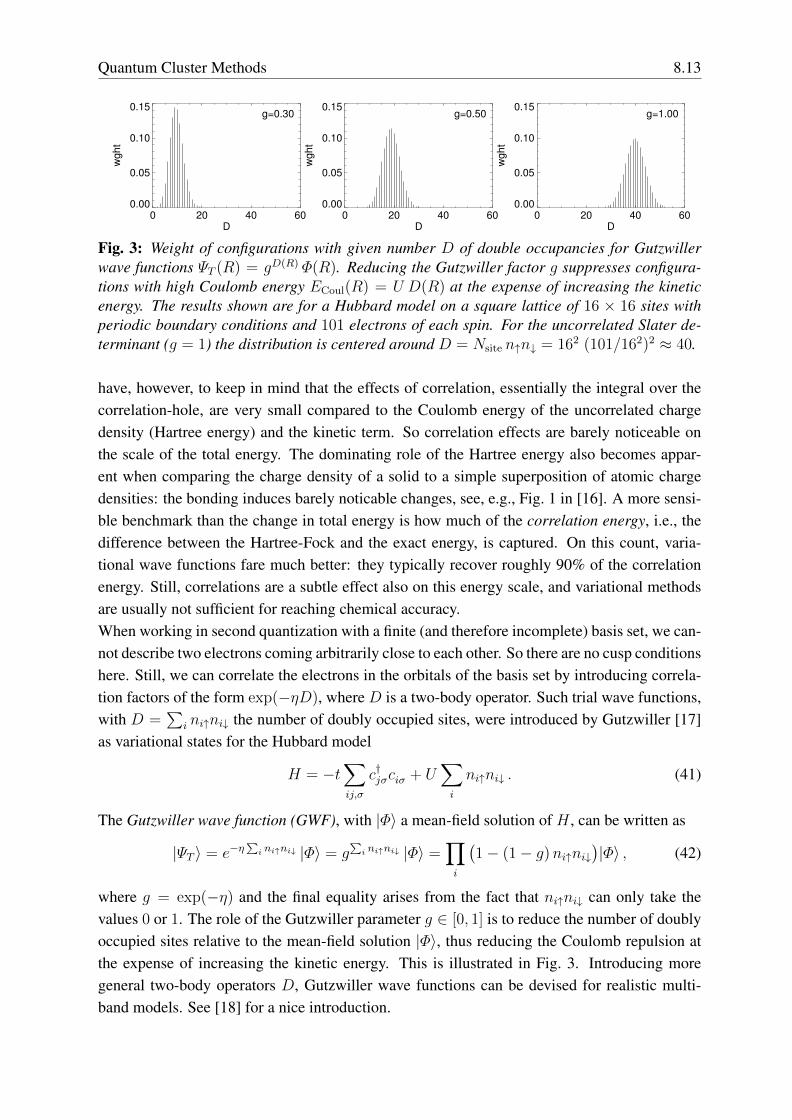
Fig. 3: Weight of configurations with given number D of double occupancies for Gutzwillerwave functions ΨT (R) = gD(R) Φ(R). Reducing the Gutzwiller factor g suppresses configura-tions with high Coulomb energy ECoul(R) = U D(R) at the expense of increasing the kineticenergy. The results shown are for a Hubbard model on a square lattice of 16 × 16 sites withperiodic boundary conditions and 101 electrons of each spin. For the uncorrelated Slater de-terminant (g = 1) the distribution is centered around D = Nsite n↑n↓ = 162 (101/162)2 ≈ 40.

have, however, to keep in mind that the effects of correlation, essentially the integral over thecorrelation-hole, are very small compared to the Coulomb energy of the uncorrelated chargedensity (Hartree energy) and the kinetic term. So correlation effects are barely noticeable onthe scale of the total energy. The dominating role of the Hartree energy also becomes appar-ent when comparing the charge density of a solid to a simple superposition of atomic chargedensities: the bonding induces barely noticable changes, see, e.g., Fig. 1 in [16]. A more sensi-ble benchmark than the change in total energy is how much of the correlation energy, i.e., thedifference between the Hartree-Fock and the exact energy, is captured. On this count, varia-tional wave functions fare much better: they typically recover roughly 90% of the correlationenergy. Still, correlations are a subtle effect also on this energy scale, and variational methodsare usually not sufficient for reaching chemical accuracy.When working in second quantization with a finite (and therefore incomplete) basis set, we can-not describe two electrons coming arbitrarily close to each other. So there are no cusp conditionshere. Still, we can correlate the electrons in the orbitals of the basis set by introducing correla-tion factors of the form exp(−ηD), where D is a two-body operator. Such trial wave functions,with D =

∑i ni↑ni↓ the number of doubly occupied sites, were introduced by Gutzwiller [17]

as variational states for the Hubbard model

H = −t∑ij,σ

c†jσciσ + U∑i

ni↑ni↓ . (41)

The Gutzwiller wave function (GWF), with |Φ〉 a mean-field solution of H , can be written as

|ΨT 〉 = e−η∑i ni↑ni↓ |Φ〉 = g

∑i ni↑ni↓ |Φ〉 =

∏i

(1− (1− g)ni↑ni↓

)|Φ〉 , (42)

where g = exp(−η) and the final equality arises from the fact that ni↑ni↓ can only take thevalues 0 or 1. The role of the Gutzwiller parameter g ∈ [0, 1] is to reduce the number of doublyoccupied sites relative to the mean-field solution |Φ〉, thus reducing the Coulomb repulsion atthe expense of increasing the kinetic energy. This is illustrated in Fig. 3. Introducing moregeneral two-body operators D, Gutzwiller wave functions can be devised for realistic multi-band models. See [18] for a nice introduction.

8.14 Erik Koch

2.1 Variational Monte Carlo

As seen in (40), evaluating the energy expectation value for a Jastrow wave function involvesthe integration over the 3N -dimensional configuration space of the electrons. The key for doingthis using stochastic sampling is again the local energy, which allows us to rewrite (40) as

〈ΨJ |H|ΨJ〉〈ΨJ |ΨJ〉

=

∫dr1 · · · drN Eloc(r1, σ1; . . . ; rN , σN) |ΨJ(r1, σ1; . . . ; rN , σN)|2∫

dr1 · · · drN |ΨJ(r1, σ1; . . . ; rN , σN)|2. (43)

As it is non-negative and normalized,

p(r1, σ1; . . . ; rN , σN) =|ΨJ(r1, σ1; . . . ; rN , σN)|2∫

dr1 · · · drN |ΨJ(r1, σ1; . . . ; rN , σN)|2(44)

is a probability distribution function on the configuration space, so that we can evaluate (43)by sampling configurations R = (r1, σ1; . . . ; rN , σN) with probability p(R) and average thecorresponding local energy Eloc(R).The same approach works for Hamiltonians written in second quantization, the main differencebeing that in this case the electron configurations are discrete, specifying the occupation ofthe orbitals used in second quantization. In the following, we specialize to the case of thesimple Hubbard model (41) with one orbital per site. Denoting by R an electron configuration,specifying on which site the electrons are located as well as their spin, we can write the energyexpectation value of a trial function ΨT as

ET =〈ΨT |H|ΨT 〉〈ΨT |ΨT 〉

=

∑REloc(R) Ψ 2

T (R)∑R Ψ

2T (R)

, (45)

with the local energy

Eloc(R) =∑R′

〈ΨT |R′〉 〈R′|H|R〉〈ΨT |R〉

=∑R′ 6=R

tΨT (R′)

ΨT (R)+ U D(R). (46)

If the Hamiltonian allows only hopping to near neighbors, the sum over R′ in the local energyscales with the number of near neighbors times the number of electrons in the system. Incontrast, the sum over R in (45) is over all configurations, i.e., of the order of the dimension ofthe Hilbert space. With increasing system size this rapidly becomes extremely large. To give animpression, the dimension of the Hilbert space for the model shown in Fig. 3 is

(162

101

)×(

162

101

),

which is larger than 10146. So it seems quite impossible to do the sum in (45). Even generatingconfigurations at a rate of 3.3 GHz, we could visit just 1017 configurations per year. It is themagic of stochastic methods that sums over such spaces can still be done to an astonishingaccuracy.The idea of variational Monte Carlo [19, 20] is to perform a random walk in the space ofconfigurations, with transition probabilities p(R → R′) chosen such that the configurationsRVMC in the random walk have the probability distribution function Ψ 2

T (R). Then

EVMC =

∑RVMC

Eloc(RVMC)∑RVMC

1≈∑

REloc(R) Ψ 2T (R)∑

R Ψ2T (R)

= ET . (47)

Quantum Cluster Methods 8.15

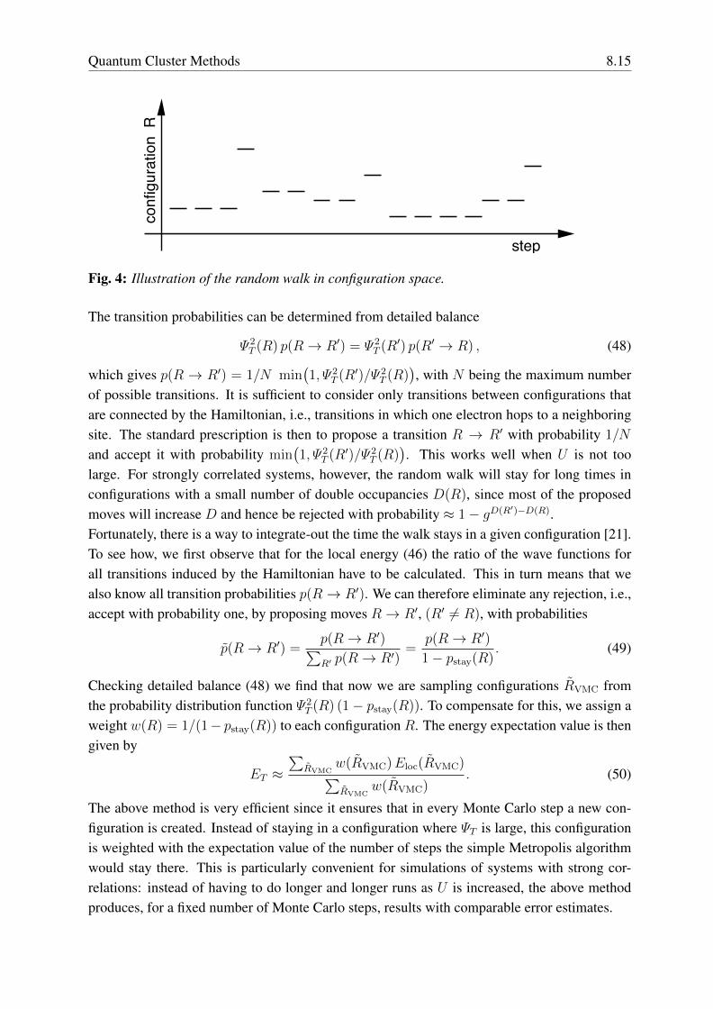
conf

igur

atio

n R

step

Fig. 4: Illustration of the random walk in configuration space.

The transition probabilities can be determined from detailed balance

Ψ 2T (R) p(R→ R′) = Ψ 2

T (R′) p(R′ → R) , (48)

which gives p(R → R′) = 1/N min(1, Ψ 2

T (R′)/Ψ 2T (R)

), with N being the maximum number

of possible transitions. It is sufficient to consider only transitions between configurations thatare connected by the Hamiltonian, i.e., transitions in which one electron hops to a neighboringsite. The standard prescription is then to propose a transition R → R′ with probability 1/N

and accept it with probability min(1, Ψ 2

T (R′)/Ψ 2T (R)

). This works well when U is not too

large. For strongly correlated systems, however, the random walk will stay for long times inconfigurations with a small number of double occupancies D(R), since most of the proposedmoves will increase D and hence be rejected with probability ≈ 1− gD(R′)−D(R).Fortunately, there is a way to integrate-out the time the walk stays in a given configuration [21].To see how, we first observe that for the local energy (46) the ratio of the wave functions forall transitions induced by the Hamiltonian have to be calculated. This in turn means that wealso know all transition probabilities p(R→ R′). We can therefore eliminate any rejection, i.e.,accept with probability one, by proposing moves R→ R′, (R′ 6= R), with probabilities

p(R→ R′) =p(R→ R′)∑R′ p(R→ R′)

=p(R→ R′)

1− pstay(R). (49)

Checking detailed balance (48) we find that now we are sampling configurations RVMC fromthe probability distribution function Ψ 2

T (R) (1− pstay(R)). To compensate for this, we assign aweight w(R) = 1/(1− pstay(R)) to each configuration R. The energy expectation value is thengiven by

ET ≈∑

RVMCw(RVMC)Eloc(RVMC)∑RVMC

w(RVMC). (50)

The above method is very efficient since it ensures that in every Monte Carlo step a new con-figuration is created. Instead of staying in a configuration where ΨT is large, this configurationis weighted with the expectation value of the number of steps the simple Metropolis algorithmwould stay there. This is particularly convenient for simulations of systems with strong cor-relations: instead of having to do longer and longer runs as U is increased, the above methodproduces, for a fixed number of Monte Carlo steps, results with comparable error estimates.

8.16 Erik Koch

2.2 Correlated sampling

The essence of the variational method is the minimization of the energy expectation value (45)as a function of the variational parameters in the trial function. To this end, we could simplyperform independent VMC calculations for a set of different parameters. It is, however, difficultto compare the energies from independent calculations since each VMC result comes with itsown statistical errors. This problem can be avoided with correlated sampling [19,22]. The ideais to use the same random walk in calculating the expectation value for different trial functions.This reduces the relative errors and hence makes it easier to find the minimum.Let us assume that we have generated a random walk {RVMC} for the trial function ΨT . Usingthe same random walk, we can also estimate the energy expectation value (47) for a differenttrial function ΨT . To do so we have to compensate for the fact that the configurations have theprobability distribution Ψ 2

T instead of Ψ 2T by introducing reweighting factors

ET ≈∑

RVMCEloc(R) Ψ 2

T (R)/Ψ 2T (R)∑

RVMCΨ 2T (R)/Ψ 2

T (R). (51)

Likewise, (50) is reweighted into

ET ≈∑

RVMCw(R) Eloc(R) Ψ 2

T (R)/Ψ 2T (R)∑

RVMCw(R) Ψ 2

T (R)/Ψ 2T (R)

. (52)

Also, the local energy Eloc(R) can be rewritten such that the new trial function appears onlyin ratios with the old one. For Gutzwiller functions this implies a drastic simplification. Sincethey differ only in the Gutzwiller factor, the Slater determinants cancel, leaving only powers(g/g)D(R)

ET (g) ≈∑

RVMCEloc(R) (g/g)2D(R)∑RVMC

(g/g)2D(R)(53)

and

Eloc(R) = −t∑R′ 6=R

(g/g)D(R′)−D(R) ΨT (R′)

ΨT (R)+ U D(R). (54)

As the number of doubly occupied sites D(R) for a configuration R is an integer, we canrearrange the sums in (53) and (54) into polynomials in g/g. The energy expectation value forany Gutzwiller parameter g is then given by a rational function in the variable g/g, where thecoefficients only depend on the fixed trial function |Ψ(g)〉.It is then clear how we proceed to optimize the Gutzwiller parameter in variational MonteCarlo [21]: we first pick a reasonable g and perform a VMC run for |Ψ(g)〉 during which wealso estimate the coefficients of the above polynomials. We can then easily calculate ET (g) byevaluating the rational function in g/g. Since the number of non-vanishing coefficients typicallyis only of the order of a few tens (see the distribution of weights shown in Figure 3), this is avery efficient process.Figure 5 shows how the method works in practice. Although we deliberately picked a badstarting point, we still find the correct minimum. Of course, this will not be true for the whole

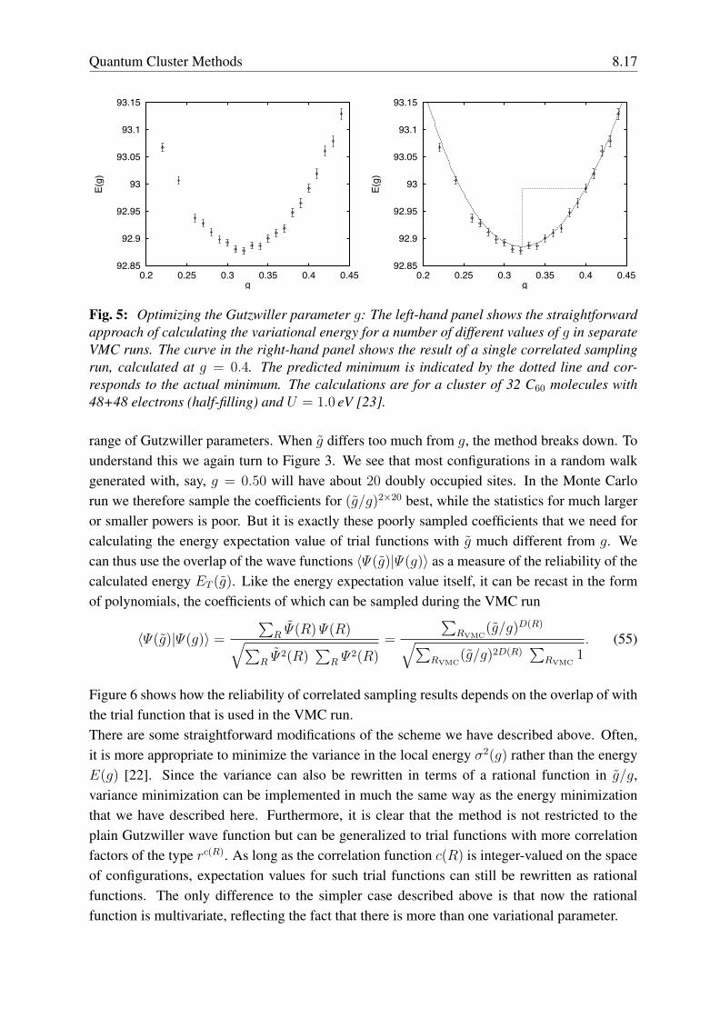
Quantum Cluster Methods 8.17

92.85

92.9

92.95

93

93.05

93.1

93.15

0.2 0.25 0.3 0.35 0.4 0.45

E(g)

g

92.85

92.9

92.95

93

93.05

93.1

93.15

0.2 0.25 0.3 0.35 0.4 0.45

E(g)

g

Fig. 5: Optimizing the Gutzwiller parameter g: The left-hand panel shows the straightforwardapproach of calculating the variational energy for a number of different values of g in separateVMC runs. The curve in the right-hand panel shows the result of a single correlated samplingrun, calculated at g = 0.4. The predicted minimum is indicated by the dotted line and cor-responds to the actual minimum. The calculations are for a cluster of 32 C60 molecules with48+48 electrons (half-filling) and U = 1.0 eV [23].

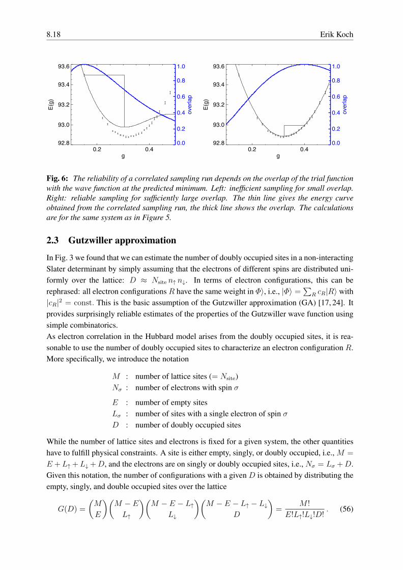
range of Gutzwiller parameters. When g differs too much from g, the method breaks down. Tounderstand this we again turn to Figure 3. We see that most configurations in a random walkgenerated with, say, g = 0.50 will have about 20 doubly occupied sites. In the Monte Carlorun we therefore sample the coefficients for (g/g)2×20 best, while the statistics for much largeror smaller powers is poor. But it is exactly these poorly sampled coefficients that we need forcalculating the energy expectation value of trial functions with g much different from g. Wecan thus use the overlap of the wave functions 〈Ψ(g)|Ψ(g)〉 as a measure of the reliability of thecalculated energy ET (g). Like the energy expectation value itself, it can be recast in the formof polynomials, the coefficients of which can be sampled during the VMC run

〈Ψ(g)|Ψ(g)〉 =

∑R Ψ(R)Ψ(R)√∑

R Ψ2(R)

∑R Ψ

2(R)=

∑RVMC

(g/g)D(R)√∑RVMC

(g/g)2D(R)∑

RVMC1. (55)

Figure 6 shows how the reliability of correlated sampling results depends on the overlap of withthe trial function that is used in the VMC run.There are some straightforward modifications of the scheme we have described above. Often,it is more appropriate to minimize the variance in the local energy σ2(g) rather than the energyE(g) [22]. Since the variance can also be rewritten in terms of a rational function in g/g,variance minimization can be implemented in much the same way as the energy minimizationthat we have described here. Furthermore, it is clear that the method is not restricted to theplain Gutzwiller wave function but can be generalized to trial functions with more correlationfactors of the type rc(R). As long as the correlation function c(R) is integer-valued on the spaceof configurations, expectation values for such trial functions can still be rewritten as rationalfunctions. The only difference to the simpler case described above is that now the rationalfunction is multivariate, reflecting the fact that there is more than one variational parameter.

8.18 Erik Koch

0.2 0.4g

92.8

93.0

93.2

93.4

93.6

E(g)

0.0

0.2

0.4

0.6

0.8

1.0

overlap

0.2 0.4g

92.8

93.0

93.2

93.4

93.6

E(g)

0.0

0.2

0.4

0.6

0.8

1.0

overlap

Fig. 6: The reliability of a correlated sampling run depends on the overlap of the trial functionwith the wave function at the predicted minimum. Left: inefficient sampling for small overlap.Right: reliable sampling for sufficiently large overlap. The thin line gives the energy curveobtained from the correlated sampling run, the thick line shows the overlap. The calculationsare for the same system as in Figure 5.

2.3 Gutzwiller approximation

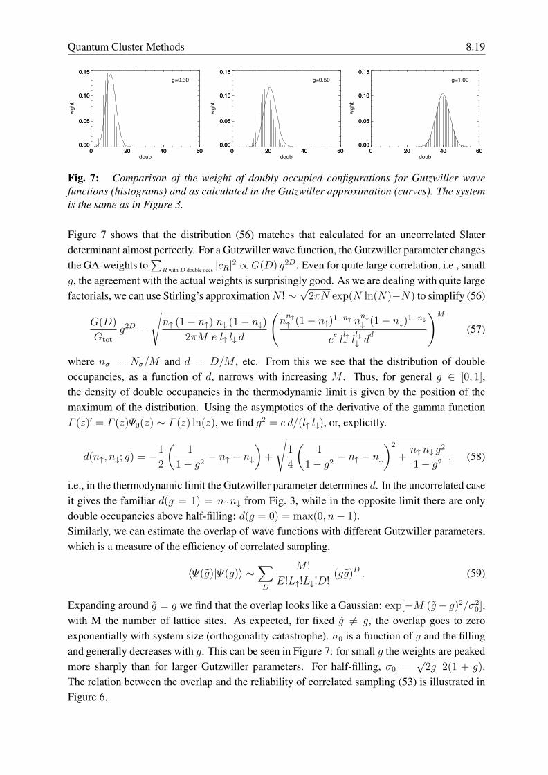
In Fig. 3 we found that we can estimate the number of doubly occupied sites in a non-interactingSlater determinant by simply assuming that the electrons of different spins are distributed uni-formly over the lattice: D ≈ Nsite n↑ n↓. In terms of electron configurations, this can berephrased: all electron configurations R have the same weight in Φ〉, i.e., |Φ〉 =

∑R cR|R〉 with

|cR|2 = const. This is the basic assumption of the Gutzwiller approximation (GA) [17, 24]. Itprovides surprisingly reliable estimates of the properties of the Gutzwiller wave function usingsimple combinatorics.As electron correlation in the Hubbard model arises from the doubly occupied sites, it is rea-sonable to use the number of doubly occupied sites to characterize an electron configuration R.More specifically, we introduce the notation

M : number of lattice sites (= Nsite)Nσ : number of electrons with spin σ

E : number of empty sitesLσ : number of sites with a single electron of spin σD : number of doubly occupied sites

While the number of lattice sites and electrons is fixed for a given system, the other quantitieshave to fulfill physical constraints. A site is either empty, singly, or doubly occupied, i.e., M =

E +L↑ +L↓ +D, and the electrons are on singly or doubly occupied sites, i.e., Nσ = Lσ +D.Given this notation, the number of configurations with a given D is obtained by distributing theempty, singly, and double occupied sites over the lattice

G(D) =

(M

E

)(M − EL↑

)(M − E − L↑

L↓

)(M − E − L↑ − L↓

D

)=

M !

E!L↑!L↓!D!. (56)

Quantum Cluster Methods 8.19

0 20 40 600.00

0.05

0.10

0.15

0 20 40 600.00

0.05

0.10

0.15

0 20 40 600.00

0.05

0.10

0.15

0 20 40 60doub

0.00

0.05

0.10

0.15wght

g=0.30

0 20 40 60doub

0.00

0.05

0.10

0.15

wght

g=0.50

0 20 40 60doub

0.00

0.05

0.10

0.15

wght

g=1.00

Fig. 7: Comparison of the weight of doubly occupied configurations for Gutzwiller wavefunctions (histograms) and as calculated in the Gutzwiller approximation (curves). The systemis the same as in Figure 3.

Figure 7 shows that the distribution (56) matches that calculated for an uncorrelated Slaterdeterminant almost perfectly. For a Gutzwiller wave function, the Gutzwiller parameter changesthe GA-weights to

∑R withD double occs |cR|2 ∝ G(D) g2D. Even for quite large correlation, i.e., small

g, the agreement with the actual weights is surprisingly good. As we are dealing with quite largefactorials, we can use Stirling’s approximationN ! ∼

√2πN exp(N ln(N)−N) to simplify (56)

G(D)

Gtot

g2D =

√n↑ (1− n↑) n↓ (1− n↓)

2πM e l↑ l↓ d

(nn↑↑ (1− n↑)1−n↑ n

n↓↓ (1− n↓)1−n↓

eell↑↑ l

l↓↓ d

d

)M

(57)

where nσ = Nσ/M and d = D/M , etc. From this we see that the distribution of doubleoccupancies, as a function of d, narrows with increasing M . Thus, for general g ∈ [0, 1],the density of double occupancies in the thermodynamic limit is given by the position of themaximum of the distribution. Using the asymptotics of the derivative of the gamma functionΓ (z)′ = Γ (z)Ψ0(z) ∼ Γ (z) ln(z), we find g2 = e d/(l↑ l↓), or, explicitly.

d(n↑, n↓; g) = −1

2

(1

1− g2− n↑ − n↓

)+

√1

4

(1

1− g2− n↑ − n↓

)2

+n↑ n↓ g2

1− g2, (58)

i.e., in the thermodynamic limit the Gutzwiller parameter determines d. In the uncorrelated caseit gives the familiar d(g = 1) = n↑ n↓ from Fig. 3, while in the opposite limit there are onlydouble occupancies above half-filling: d(g = 0) = max(0, n− 1).Similarly, we can estimate the overlap of wave functions with different Gutzwiller parameters,which is a measure of the efficiency of correlated sampling,

〈Ψ(g)|Ψ(g)〉 ∼∑D

M !

E!L↑!L↓!D!(gg)D . (59)

Expanding around g = g we find that the overlap looks like a Gaussian: exp[−M (g− g)2/σ20],

with M the number of lattice sites. As expected, for fixed g 6= g, the overlap goes to zeroexponentially with system size (orthogonality catastrophe). σ0 is a function of g and the fillingand generally decreases with g. This can be seen in Figure 7: for small g the weights are peakedmore sharply than for larger Gutzwiller parameters. For half-filling, σ0 =

√2g 2(1 + g).

The relation between the overlap and the reliability of correlated sampling (53) is illustrated inFigure 6.

8.20 Erik Koch

For the energy expectation value

E(g) =〈Ψ(g)|H|Ψ(g)〉〈Ψ(g)|Ψ(g)〉

= −2t∑ij,σ

〈Ψ(g)|c†jσciσ|Ψ(g)〉〈Ψ(g)|Ψ(g)〉

+ U D(g) (60)

in the Gutzwiller approximation, the Hubbard energy is explicitly given through the relation (58)between g and the density of doubly occupied sites. For estimating the kinetic energy, we firstobserve that 〈Ψ(g)|c†jσciσ|Ψ(g)〉/〈Ψ(g)|Ψ(g)〉 is the probability for an electron of spin σ tohop from site i to site j. The probability for a hop being allowed by the Pauli principle isnσ (1− nσ). In the Gutzwiller approximation there are more severe constraints on the hoppingprocesses coming from the condition that the density of doubly occupied sites is fixed at (58).Thus, only hops from a singly occupied to an empty site (probability lσ e) or from a doubly toa singly occupied site (probability d l−σ) are allowed. Thus, replacing the Pauli constraint withthe more severe Gutzwiller constraints reduces the hopping matrix elements of the uncorrelatedSlater determinant by the hopping reduction factor

γσ(nσ, g) =

(√lσ e+

√d l−σ

)2

nσ (1− nσ), (61)

where we have added the amplitudes for the two allowed hopping processes. Using again thebasic assumption of the Gutzwiller approximation that all configurations contribute the same,we find for the energy per site

εGA(g) =∑σ

γσ(nσ, g) ε(0)σ (nσ) + U d(n↑, n↓; g) , (62)

where ε0σ(nσ) is the kinetic energy for the Slater determinant of the Gutzwiller wave functions.

Optimizing the Gutzwiller parameter g thus means finding the best trade-off between loweringthe Hubbard energy by reducing the density of double occupancies and the simultaneous in-crease in the (negative) kinetic energy due to the band narrowing proportional to the hoppingreduction γσ. Because of the relation (58) between g and d we actually need not consider g butcan minimize the energy using d as the parameter.

2.4 Brinkman-Rice transition

At half-filling (nσ = 1/2) the expressions from the Gutzwiller approximation simplify signifi-cantly. The hopping reduction factor becomes γ = 16d(1/2 − d), so we can write the energyexpectation value per site as

ε(d) = 16 d (1/2− d) ε(0) + U d , (63)

where ε(0) is the kinetic energy density of the uncorrelated system (both spins). Minimizinggives

dmin(U) =1

4+

U

32ε(0). (64)

Quantum Cluster Methods 8.21

0

1

2

3

4

5

6

7

8

9

6 7 8 9 10 11 12 13 14

Eg /

t

U / t

30 sites 50 sites 70 sites 90 sites110 sites130 sites

GA

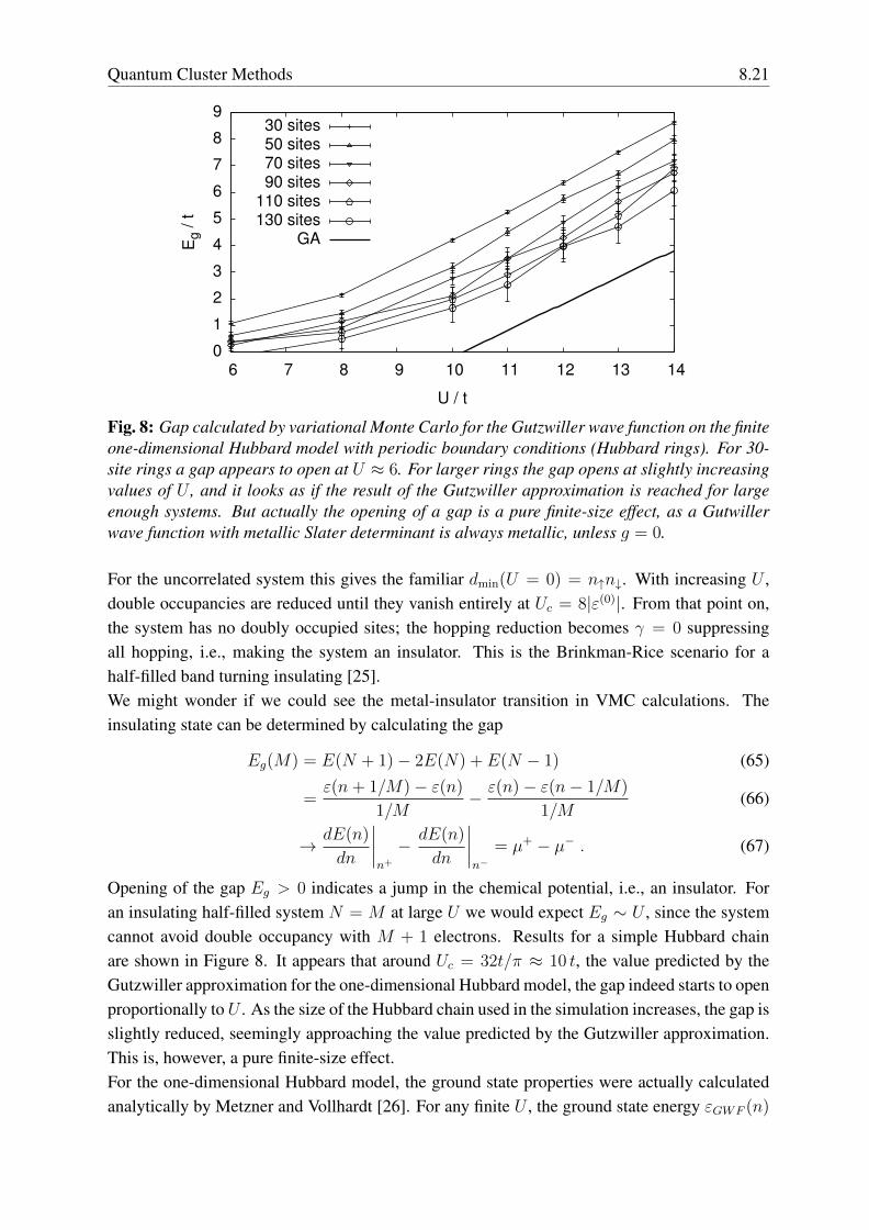
Fig. 8: Gap calculated by variational Monte Carlo for the Gutzwiller wave function on the finiteone-dimensional Hubbard model with periodic boundary conditions (Hubbard rings). For 30-site rings a gap appears to open at U ≈ 6. For larger rings the gap opens at slightly increasingvalues of U , and it looks as if the result of the Gutzwiller approximation is reached for largeenough systems. But actually the opening of a gap is a pure finite-size effect, as a Gutwillerwave function with metallic Slater determinant is always metallic, unless g = 0.

For the uncorrelated system this gives the familiar dmin(U = 0) = n↑n↓. With increasing U ,double occupancies are reduced until they vanish entirely at Uc = 8|ε(0)|. From that point on,the system has no doubly occupied sites; the hopping reduction becomes γ = 0 suppressingall hopping, i.e., making the system an insulator. This is the Brinkman-Rice scenario for ahalf-filled band turning insulating [25].We might wonder if we could see the metal-insulator transition in VMC calculations. Theinsulating state can be determined by calculating the gap

Eg(M) = E(N + 1)− 2E(N) + E(N − 1) (65)

=ε(n+ 1/M)− ε(n)

1/M− ε(n)− ε(n− 1/M)

1/M(66)

→ dE(n)

dn

∣∣∣∣n+

− dE(n)

dn

∣∣∣∣n−

= µ+ − µ− . (67)

Opening of the gap Eg > 0 indicates a jump in the chemical potential, i.e., an insulator. Foran insulating half-filled system N = M at large U we would expect Eg ∼ U , since the systemcannot avoid double occupancy with M + 1 electrons. Results for a simple Hubbard chainare shown in Figure 8. It appears that around Uc = 32t/π ≈ 10 t, the value predicted by theGutzwiller approximation for the one-dimensional Hubbard model, the gap indeed starts to openproportionally to U . As the size of the Hubbard chain used in the simulation increases, the gap isslightly reduced, seemingly approaching the value predicted by the Gutzwiller approximation.This is, however, a pure finite-size effect.For the one-dimensional Hubbard model, the ground state properties were actually calculatedanalytically by Metzner and Vollhardt [26]. For any finite U , the ground state energy εGWF (n)

8.22 Erik Koch

has a continuous derivative at half-filling. So the Gutzwiller wave function always describes ametal, except for g = 0. This example should serve as a warning that finite-size extrapolationscan be quite tricky. Here, even though the energy per site converges quickly to the exact result,having to take finite differences instead of derivatives in the evaluation of the gap for finitesystems can create the appearance of a gapped system.There is an elegant argument using the response of the energy to twisted boundary conditionsthat shows that, quite generally, Gutzwiller-type wave functions with a metallic Slater determi-nant are always metallic [27]. Consider a variational wave function

|Ψ〉 =∏α

gCαα |Φ〉 , (68)

where |Φ〉 is a Slater determinant and Cα a set of correlation functions (the simple Gutzwillerfunction uses only one correlation function,

∑i ni↑ni↓). For twisted boundary conditions in

direction c on a finite simulation cell, moving an electron by the cell vector c = An introducesa phase exp(ik · c). This phase can be absorbed into the Hamiltonian by transforming the cre-ation/annihilation operators at site Aj into cjσ → eik·Aj cjσ and introducing periodic boundaryconditions. The Hamiltonian thus becomes dependent on k with the hopping terms picking up aphase from the twisted boundary conditions, while in the Hubbard interaction the phases cancel

H(k) = −t∑ij,σ

eik·A(i−j) c†jσciσ + U∑i

ni↑ ni↓ . (69)

The energy expectation value for the Gutzwiller wave function depends on k and the gα, wherethe Gutzwiller parameters change with the boundary conditions as

EG(k+dk, {gα(k+dk)}) = EG(k, {gα(k)})+

(∂EG∂k

+∑α

∂EG∂gα

dgαdk

)dk+O(dk2). (70)

The Gutzwiller parameters minimize EG, i.e., the variations of the energy expectation valuewith respect to the gα vanish. Solving the resulting linear system for the first-order term givesthe dependence of the Gutzwiller parameters on the boundary conditions

dgαdk

= −∑β

(∂2EG∂gβ ∂gα

)−1(∂2EG∂gβ ∂k

), (71)

while the second derivative of the energy with respect to the boundary conditions is

d2EGdk2

=d

dk

(∂EG∂k

+∑α

∂EG∂gα

dgαdk

)=∂2EG∂k2

+∑α

∂2EG∂k ∂gα

dgαdk

. (72)

When the Gutzwiller factors in (68) are independent of the boundary conditions, e.g., the Ci aredensity or spin correlation functions, the explicit dependence of EG on the boundary conditionsk is only through the kinetic energy T . For a metallic Slater determinant the first term will thenproduce a non-vanishing conductivity for any U , except in the atomic limit U →∞.The Brinkman-Rice transition is thus produced by the Gutzwiller approximation, although it isnot present in the underlying Gutzwiller wave function, except in the limit d → ∞, where theGutzwiller approximation becomes exact [26].

Quantum Cluster Methods 8.23

3 Projection techniques

We can systematically improve on the variational results by using projection techniques [28].The basic idea is surprisingly simple: when we operate with exp(−τH) on a wave function|ΨT 〉 then, for large τ , the ground state |ψ0〉 will dominate in the projected function, providedthat the initial function had non-zero overlap with it. For a finite-dimensional Hamiltonian,where the spectrum is bounded not only from below but also from above, this imaginary-timepropagation can be simplified to a matrix vector product

|Ψ (n+1)〉 = [1− τ(H − E(n))] |Ψ (n)〉 ; |Ψ (0)〉 = |ΨT 〉, (73)

where τ has to be small enough and E(n) is chosen to ensure normalization of the projectedfunctions. To see under what conditions this converges to the ground state, we expand thestarting function |ΨT 〉 =

∑i ci|Ψi〉 in eigenstates H|Ψi〉 = Ei|Ψi〉. Then

|Ψ (n)〉 =∑

ci∏n

[1− τ(Ei − E(n))]|Ψi〉 . (74)

Convergence to |Ψ0〉, up to normalization, is ensured if ci 6= 0 and

|1− τ(E0 − E(n))| > |1− τ(Ei − E(n))| ∀i 6= 0 . (75)

For τ > 0 we distinguish two cases

• 1− τ(E0 − E(n)) > 1− τ(Ei − E(n)), which leads to the trivial E0 < Ei, and

• 1−τ(E0−E(n)) > −[1−τ(Ei−E(n))], from which follows that 2 > τ(Ei+E0−2E(n)).

Thus, to secure convergence, one has to choose

0 < τ <2

Emax + E0 − 2E(n)(76)

which implies that E(n) ∈ [E0, Emax] must lie inside the spectrum of H . In fact, for large n itwill approach the ground state energy.Because of the prohibitively large dimension of the many-body Hilbert space, the matrix vectorproduct in (73) cannot be done exactly. Instead, we rewrite the equation in configuration space∑

R′

|R′〉〈R′|Ψ (n+1)〉 =∑R,R′

|R′〉 〈R′|1− τ(H − E0)|R〉︸ ︷︷ ︸=:F (R′,R)

〈R|Ψ (n)〉 (77)

and perform the propagation in a stochastic sense: |Ψ (n)〉 is represented by an ensemble ofconfigurations R with weights w(R). The transition matrix element F (R′, R) is rewritten asa transition probability p(R → R′) times a normalization factor m(R′, R). The iteration (77)is then stochastically performed as follows: for each R we pick, out of the set of all allowedconfigurations, one new configurationR′ with probability p(R→ R′) and multiply its weight bym(R′, R). Then the new ensemble of configurations R′ with their respective weights representsthe new function |Ψ (n+1)〉.

8.24 Erik Koch

3.1 Importance sampling

Importance sampling introduces a guiding function |ΨG〉 to decisively improve the efficiency ofthe stochastic projection by enhancing transitions from configurations where the trial function issmall to configurations with large trial function, i.e., by replacing the transition matrix elementF (R′, R) with G(R′, R) = 〈R′|ΨG〉F (R′, R)/〈R|ΨG〉. The propagation is then given by∑

R′

|R′〉〈R′|ΨG〉〈R′|Ψ (n+1)〉 =∑R,R′

|R′〉G(R′, R) 〈R|ΨG〉 〈R|Ψ (n)〉 (78)

and the ensemble of configurations now represents the product ΨG Ψ (n). This means that theprobability distribution function P (n)(w,R) dw of configurations R with weight w is such that

ΨG(R)Ψ (n)(R) =

∫wP (n)(w,R) dw . (79)

To see this, we rewrite the matrix element of the propagation as

G(R′, R) = p(R→ R′)m(R′, R) , (80)

where p(R → R′) is the probability for the random walk to move from configuration R toR′ and the weight m(R′, R) takes care of the normalization. For the probability distributionfunction this implies

P (n+1)(w′, R′) dw′ =∑R

p(R→ R′) P (n)

(w′

m(R′, R), R

)dw′

m(R′, R)(81)

and hence∫w′ P (n+1)(w′, R′) dw′ =

∑R

p(R→ R′)

∫w′ P (n)

(w′

m(R′, R), R

)dw′

m(R′R)

=∑R

p(R→ R′)m(R′, R)

∫wP (n)(w,R) dw

=∑R

G(R′, R) ΨG(R)Ψ (n)(R)

= ΨG(R′)Ψ (n+1)(R′) .

After a large number n of iterations, the ground-state energy is given by the mixed estimator

E(n)0 =

〈ΨG|H|Ψ (n)〉〈ΨG|Ψ (n)〉

≈∑

REloc(R) w(n)(R)∑R w

(n)(R). (82)

When we start the iteration from the guiding function, we can generate the configurations for theinitial state ΨG(R)Ψ (0)(R) by a variational Monte Carlo run for ΨG. For this practical reasonone usually choses the guiding function to be the VMC trial function. In the following wetherefore use ΨG and ΨT synonymously.

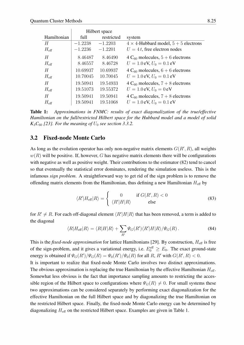
Quantum Cluster Methods 8.25

Hilbert spaceHamiltonian full restricted systemH −1.2238 −1.2203 4× 4-Hubbard model, 5 + 5 electronsHeff −1.2236 −1.2201 U = 4 t, free electron nodes

H 8.46487 8.46490 4 C60 molecules, 5 + 6 electronsHeff 8.46557 8.46728 U = 1.0 eV, U0 = 0.1 eVH 10.69937 10.69937 4 C60 molecules, 6 + 6 electronsHeff 10.70045 10.70045 U = 1.0 eV, U0 = 0.1 eVH 19.50941 19.54933 4 C60 molecules, 7 + 8 electronsHeff 19.51073 19.55372 U = 1.0 eV, U0 = 0 eVH 19.50941 19.50941 4 C60 molecules, 7 + 8 electronsHeff 19.50941 19.51068 U = 1.0 eV, U0 = 0.1 eV

Table 1: Approximations in FNMC: results of exact diagonalization of the true/effectiveHamiltonian on the full/restricted Hilbert space for the Hubbard model and a model of solidK3C60 [23]. For the meaning of U0 see section 3.3.2.

3.2 Fixed-node Monte Carlo

As long as the evolution operator has only non-negative matrix elements G(R′, R), all weightsw(R) will be positive. If, however, G has negative matrix elements there will be configurationswith negative as well as positive weight. Their contributions to the estimator (82) tend to cancelso that eventually the statistical error dominates, rendering the simulation useless. This is theinfamous sign problem. A straightforward way to get rid of the sign problem is to remove theoffending matrix elements from the Hamiltonian, thus defining a new Hamiltonian Heff by

〈R′|Heff |R〉 =

{0 if G(R′, R) < 0

〈R′|H|R〉 else(83)

for R′ 6= R. For each off-diagonal element 〈R′|H|R〉 that has been removed, a term is added tothe diagonal

〈R|Heff |R〉 = 〈R|H|R〉+∑R′

ΨG(R′)〈R′|H|R〉/ΨG(R) . (84)

This is the fixed-node approximation for lattice Hamiltonians [29]. By construction, Heff is freeof the sign-problem, and it gives a variational energy, i.e. Eeff

0 ≥ E0. The exact ground-stateenergy is obtained if ΨG(R′)/ΨG(R) = Ψ0(R′)/Ψ0(R) for all R, R′ with G(R′, R) < 0.It is important to realize that fixed-node Monte Carlo involves two distinct approximations.The obvious approximation is replacing the true Hamiltonian by the effective Hamiltonian Heff .Somewhat less obvious is the fact that importance sampling amounts to restricting the acces-sible region of the Hilbert space to configurations where ΨG(R) 6= 0. For small systems thesetwo approximations can be considered separately by performing exact diagonalization for theeffective Hamiltonian on the full Hilbert space and by diagonalizing the true Hamiltonian onthe restricted Hilbert space. Finally, the fixed-node Monte Carlo energy can be determined bydiagonalizing Heff on the restricted Hilbert space. Examples are given in Table 1.

8.26 Erik Koch

92.7

92.71

92.72

92.73

92.74

92.75

92.76

92.77

92.78

92.79

92.8

0.2 0.25 0.3 0.35 0.4 0.45

E(g

)

g

92.7

92.75

92.8

92.85

92.9

92.95

93

93.05

93.1

93.15

0.2 0.25 0.3 0.35 0.4 0.45

E(g

)

g

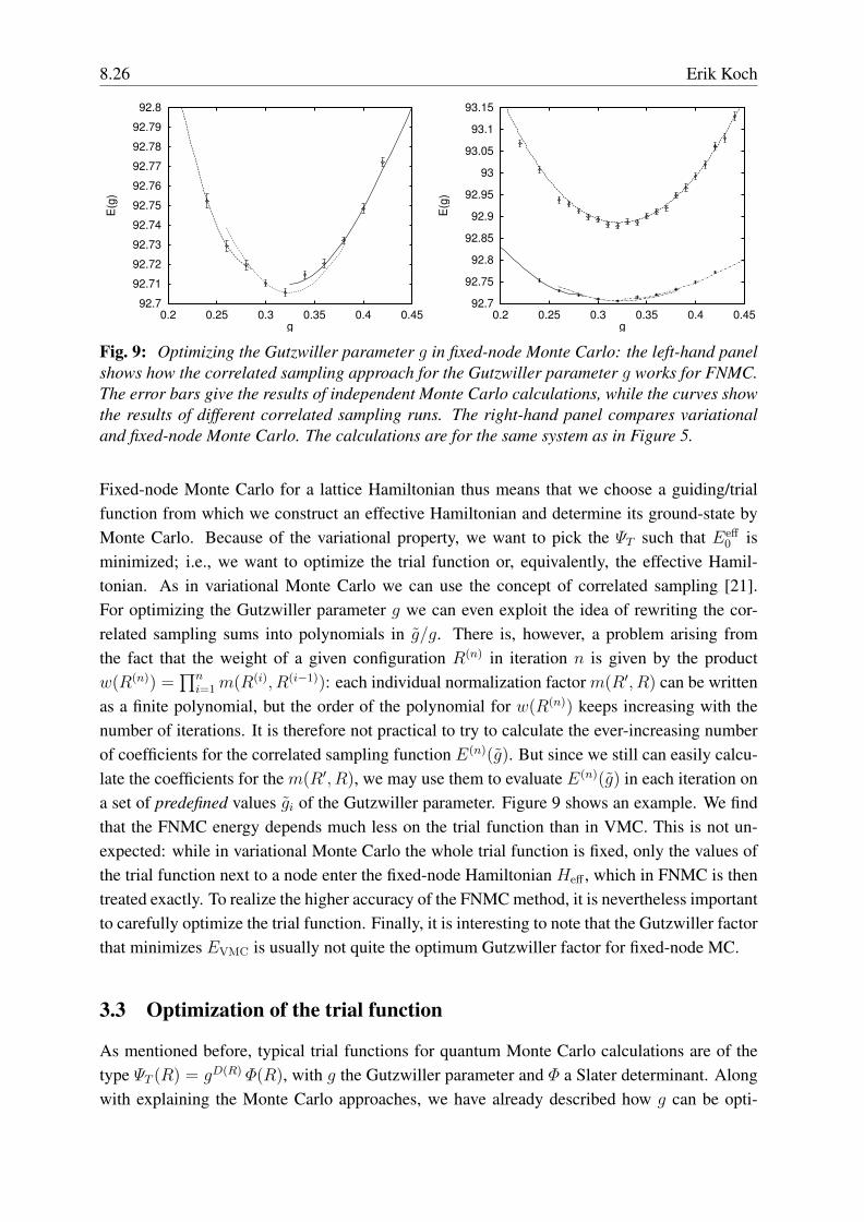
Fig. 9: Optimizing the Gutzwiller parameter g in fixed-node Monte Carlo: the left-hand panelshows how the correlated sampling approach for the Gutzwiller parameter g works for FNMC.The error bars give the results of independent Monte Carlo calculations, while the curves showthe results of different correlated sampling runs. The right-hand panel compares variationaland fixed-node Monte Carlo. The calculations are for the same system as in Figure 5.

Fixed-node Monte Carlo for a lattice Hamiltonian thus means that we choose a guiding/trialfunction from which we construct an effective Hamiltonian and determine its ground-state byMonte Carlo. Because of the variational property, we want to pick the ΨT such that Eeff

0 isminimized; i.e., we want to optimize the trial function or, equivalently, the effective Hamil-tonian. As in variational Monte Carlo we can use the concept of correlated sampling [21].For optimizing the Gutzwiller parameter g we can even exploit the idea of rewriting the cor-related sampling sums into polynomials in g/g. There is, however, a problem arising fromthe fact that the weight of a given configuration R(n) in iteration n is given by the productw(R(n)) =

∏ni=1m(R(i), R(i−1)): each individual normalization factor m(R′, R) can be written

as a finite polynomial, but the order of the polynomial for w(R(n)) keeps increasing with thenumber of iterations. It is therefore not practical to try to calculate the ever-increasing numberof coefficients for the correlated sampling function E(n)(g). But since we still can easily calcu-late the coefficients for the m(R′, R), we may use them to evaluate E(n)(g) in each iteration ona set of predefined values gi of the Gutzwiller parameter. Figure 9 shows an example. We findthat the FNMC energy depends much less on the trial function than in VMC. This is not un-expected: while in variational Monte Carlo the whole trial function is fixed, only the values ofthe trial function next to a node enter the fixed-node Hamiltonian Heff , which in FNMC is thentreated exactly. To realize the higher accuracy of the FNMC method, it is nevertheless importantto carefully optimize the trial function. Finally, it is interesting to note that the Gutzwiller factorthat minimizes EVMC is usually not quite the optimum Gutzwiller factor for fixed-node MC.

3.3 Optimization of the trial function

As mentioned before, typical trial functions for quantum Monte Carlo calculations are of thetype ΨT (R) = gD(R) Φ(R), with g the Gutzwiller parameter and Φ a Slater determinant. Alongwith explaining the Monte Carlo approaches, we have already described how g can be opti-

Quantum Cluster Methods 8.27

mized. The fundamental idea was that, for the reweighting in correlated sampling, only ratiosof the new and old trial functions are needed so that the weights and energies appearing in theMonte Carlo calculation can be recast in the form of polynomials in the ratio of the Gutzwillerparameters. In the following, we discuss generalizations of this approach to trial functionswith several Gutzwiller parameters. After that, we address the optimization of the other partof a Gutzwiller wave function: the Slater determinant. In particular, we demonstrate how thecharacter of the Slater determinant affects the result of the Monte Carlo calculation.

3.3.1 More Gutzwiller parameters

To study the static dielectric screening [30], we have to determine the response of the chargedensity to the introduction of a test charge q placed on molecule iq. To describe the test charge,the term

H1(q) = qU∑mσ

niqmσ (85)

is added to the Hamiltonian. In the spirit of the Gutzwiller ansatz, we correspondingly add asecond Gutzwiller factor to the wave function that reflects the additional interaction term qUNiq

|ΨT (g, h)〉 = gDhNiq |Φ〉. (86)

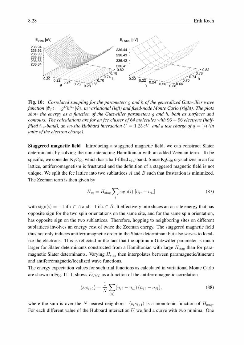
Finding the best Gutzwiller parameters is now a two-dimensional optimization problem. Deal-ing with polynomials in the two variables g and h, the method of correlated sampling works asstraightforwardly as described above for the case of a plain Gutzwiller wave function. As an ex-ample, Fig. 10 shows the result of the optimization, both in variational and in fixed-node MonteCarlo, for a cluster of 64 C60 molecules in an fcc arrangement (periodic boundary conditions)resembling K3C60 with a test charge q = 1/4. In practice, we first optimize the parameters invariational Monte Carlo. We then use the optimum VMC parameters as starting points for theoptimization in the more time-consuming fixed-node Monte Carlo calculations.

3.3.2 Variation of the Slater determinant

In the traditional Gutzwiller ansatz, the Slater determinant Φ is the ground-state wave func-tion of the non-interacting Hamiltonian. This is, however, not necessarily the best choice. Analternative would be to use the Slater determinant Φ(U) obtained by solving the interactingproblem in the Hartree-Fock approximation. We can even interpolate between the two extremesby doing a Hartree-Fock calculation with a fictitious Hubbard interaction U0 to obtain Slaterdeterminants Φ(U0). Yet another family of Slater determinants Φ(Hstag) can be obtained fromsolving the non-interacting Hamiltonian with an added staggered magnetic field, which lets uscontrol the antiferromagnetic character of the trial function. Although optimizing parametersin the Slater determinant is not possible with the method described in the preceding sections,an efficient optimization of the Gutzwiller factors makes it possible to optimize the overall trialfunction without too much effort.

8.28 Erik Koch

0.20 0.22 0.24 0.26 0.28g 0.66

0.70

0.74

0.78

0.82

h

236.84

236.86

236.88

236.90

236.92

236.94

EVMC [eV]

0.20 0.22 0.24 0.26 0.28g 0.66

0.70

0.74

0.78

0.82

h

236.41

236.42

236.43

236.44

EFNMC [eV]

Fig. 10: Correlated sampling for the parameters g and h of the generalized Gutzwiller wavefunction |ΨT 〉 = gDhNc |Φ〉, in variational (left) and fixed-node Monte Carlo (right). The plotsshow the energy as a function of the Gutzwiller parameters g and h, both as surfaces andcontours. The calculations are for an fcc cluster of 64 molecules with 96 + 96 electrons (half-filled t1u-band), an on-site Hubbard interaction U = 1.25 eV , and a test charge of q = 1/4 (inunits of the electron charge).

Staggered magnetic field Introducing a staggered magnetic field, we can construct Slaterdeterminants by solving the non-interacting Hamiltonian with an added Zeeman term. To bespecific, we consider K3C60, which has a half-filled t1u-band. Since K3C60 crystallizes in an fcclattice, antiferromagnetism is frustrated and the definition of a staggered magnetic field is notunique. We split the fcc lattice into two sublattices A and B such that frustration is minimized.The Zeeman term is then given by

Hm = Hstag

∑i

sign(i) [ni↑ − ni↓] (87)

with sign(i) = +1 if i ∈ A and −1 if i ∈ B. It effectively introduces an on-site energy that hasopposite sign for the two spin orientations on the same site, and for the same spin orientation,has opposite sign on the two sublattices. Therefore, hopping to neighboring sites on differentsublattices involves an energy cost of twice the Zeeman energy. The staggered magnetic fieldthus not only induces antiferromagnetic order in the Slater determinant but also serves to local-ize the electrons. This is reflected in the fact that the optimum Gutzwiller parameter is muchlarger for Slater determinants constructed from a Hamiltonian with large Hstag than for para-magnetic Slater determinants. Varying Hstag then interpolates between paramagnetic/itinerantand antiferromagnetic/localized wave functions.The energy expectation values for such trial functions as calculated in variational Monte Carloare shown in Fig. 11. It shows EVMC as a function of the antiferromagnetic correlation

〈sisi+1〉 =1

N

∑〈ij〉

(ni↑ − ni↓) (nj↑ − nj↓), (88)

where the sum is over the N nearest neighbors. 〈sisi+1〉 is a monotonic function of Hstag.For each different value of the Hubbard interaction U we find a curve with two minima. One

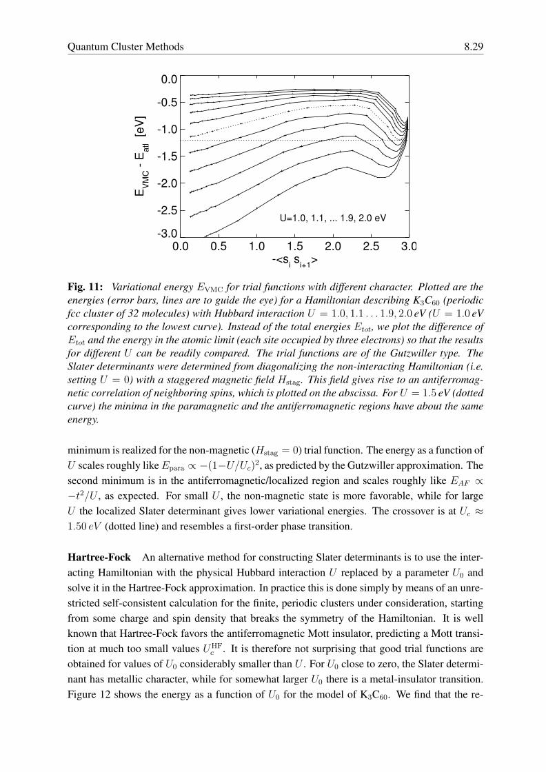
Quantum Cluster Methods 8.29

0.0 0.5 1.0 1.5 2.0 2.5 3.0-<s

i s

i+1>

-3.0

-2.5

-2.0

-1.5

-1.0

-0.5

0.0

EV

MC -

Ea

tl [e

V]

U=1.0, 1.1, ... 1.9, 2.0 eV

Fig. 11: Variational energy EVMC for trial functions with different character. Plotted are theenergies (error bars, lines are to guide the eye) for a Hamiltonian describing K3C60 (periodicfcc cluster of 32 molecules) with Hubbard interaction U = 1.0, 1.1 . . . 1.9, 2.0 eV (U = 1.0 eVcorresponding to the lowest curve). Instead of the total energies Etot, we plot the difference ofEtot and the energy in the atomic limit (each site occupied by three electrons) so that the resultsfor different U can be readily compared. The trial functions are of the Gutzwiller type. TheSlater determinants were determined from diagonalizing the non-interacting Hamiltonian (i.e.setting U = 0) with a staggered magnetic field Hstag. This field gives rise to an antiferromag-netic correlation of neighboring spins, which is plotted on the abscissa. For U = 1.5 eV (dottedcurve) the minima in the paramagnetic and the antiferromagnetic regions have about the sameenergy.

minimum is realized for the non-magnetic (Hstag = 0) trial function. The energy as a function ofU scales roughly likeEpara ∝ −(1−U/Uc)2, as predicted by the Gutzwiller approximation. Thesecond minimum is in the antiferromagnetic/localized region and scales roughly like EAF ∝−t2/U , as expected. For small U , the non-magnetic state is more favorable, while for largeU the localized Slater determinant gives lower variational energies. The crossover is at Uc ≈1.50 eV (dotted line) and resembles a first-order phase transition.

Hartree-Fock An alternative method for constructing Slater determinants is to use the inter-acting Hamiltonian with the physical Hubbard interaction U replaced by a parameter U0 andsolve it in the Hartree-Fock approximation. In practice this is done simply by means of an unre-stricted self-consistent calculation for the finite, periodic clusters under consideration, startingfrom some charge and spin density that breaks the symmetry of the Hamiltonian. It is wellknown that Hartree-Fock favors the antiferromagnetic Mott insulator, predicting a Mott transi-tion at much too small values UHF

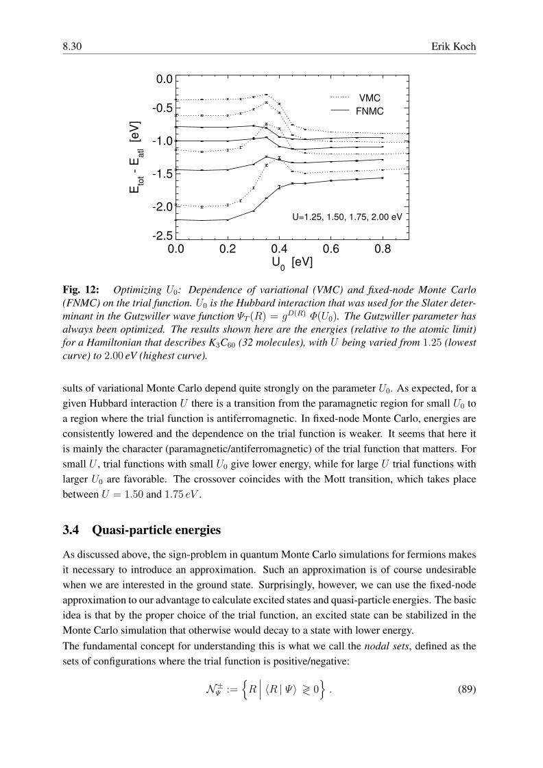
c . It is therefore not surprising that good trial functions areobtained for values of U0 considerably smaller than U . For U0 close to zero, the Slater determi-nant has metallic character, while for somewhat larger U0 there is a metal-insulator transition.Figure 12 shows the energy as a function of U0 for the model of K3C60. We find that the re-

8.30 Erik Koch

0.0 0.2 0.4 0.6 0.8U

0 [eV]

-2.5

-2.0

-1.5

-1.0

-0.5

0.0

Eto

t - E

atl [e

V]

U=1.25, 1.50, 1.75, 2.00 eV

VMC

FNMC

Fig. 12: Optimizing U0: Dependence of variational (VMC) and fixed-node Monte Carlo(FNMC) on the trial function. U0 is the Hubbard interaction that was used for the Slater deter-minant in the Gutzwiller wave function ΨT (R) = gD(R) Φ(U0). The Gutzwiller parameter hasalways been optimized. The results shown here are the energies (relative to the atomic limit)for a Hamiltonian that describes K3C60 (32 molecules), with U being varied from 1.25 (lowestcurve) to 2.00 eV (highest curve).

sults of variational Monte Carlo depend quite strongly on the parameter U0. As expected, for agiven Hubbard interaction U there is a transition from the paramagnetic region for small U0 toa region where the trial function is antiferromagnetic. In fixed-node Monte Carlo, energies areconsistently lowered and the dependence on the trial function is weaker. It seems that here itis mainly the character (paramagnetic/antiferromagnetic) of the trial function that matters. Forsmall U , trial functions with small U0 give lower energy, while for large U trial functions withlarger U0 are favorable. The crossover coincides with the Mott transition, which takes placebetween U = 1.50 and 1.75 eV .

3.4 Quasi-particle energies

As discussed above, the sign-problem in quantum Monte Carlo simulations for fermions makesit necessary to introduce an approximation. Such an approximation is of course undesirablewhen we are interested in the ground state. Surprisingly, however, we can use the fixed-nodeapproximation to our advantage to calculate excited states and quasi-particle energies. The basicidea is that by the proper choice of the trial function, an excited state can be stabilized in theMonte Carlo simulation that otherwise would decay to a state with lower energy.The fundamental concept for understanding this is what we call the nodal sets, defined as thesets of configurations where the trial function is positive/negative:

N±Ψ :={R∣∣∣ 〈R | Ψ〉 ≷ 0

}. (89)

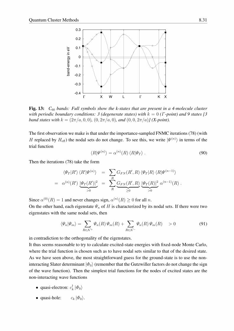
Quantum Cluster Methods 8.31

-0.4

-0.3

-0.2

-0.1

0

0.1

0.2

0.3

K X W L K K X

band

-ene

rgy

in e

V

Fig. 13: C60 bands: Full symbols show the k-states that are present in a 4-molecule clusterwith periodic boundary conditions: 3 (degenerate states) with k = 0 (Γ -point) and 9 states [3band states with k = (2π/a, 0, 0), (0, 2π/a, 0), and (0, 0, 2π/a)] (X-point).

The first observation we make is that under the importance-sampled FNMC iterations (78) (withH replaced by Heff) the nodal sets do not change. To see this, we write |Ψ (n)〉 in terms of thetrial function

〈R|Ψ (n)〉 = α(n)(R) 〈R|ΨT 〉 . (90)

Then the iterations (78) take the form

〈ΨT |R′〉 〈R′|Ψ (n)〉 =∑R

GFN(R′, R) 〈ΨT |R〉 〈R|Ψ (n−1)〉

= α(n)(R′) |ΨT (R′)|2︸ ︷︷ ︸>0

=∑R

GFN(R′, R)︸ ︷︷ ︸≥0

|ΨT (R)|2︸ ︷︷ ︸>0

α(n−1)(R) .

Since α(0)(R) = 1 and never changes sign, α(n)(R) ≥ 0 for all n.On the other hand, each eigenstate Ψn of H is characterized by its nodal sets. If there were twoeigenstates with the same nodal sets, then

〈Ψn|Ψm〉 =∑R∈N+

Ψn(R)Ψm(R) +∑R∈N−

Ψn(R)Ψm(R) > 0 (91)

in contradiction to the orthogonality of the eigenstates.It thus seems reasonable to try to calculate excited-state energies with fixed-node Monte Carlo,where the trial function is chosen such as to have nodal sets similar to that of the desired state.As we have seen above, the most straightforward guess for the ground-state is to use the non-interacting Slater determinant |Φ0〉 (remember that the Gutzwiller factors do not change the signof the wave function). Then the simplest trial functions for the nodes of excited states are thenon-interacting wave functions

• quasi-electron: c†k |Φ0〉

• quasi-hole: ck |Φ0〉.

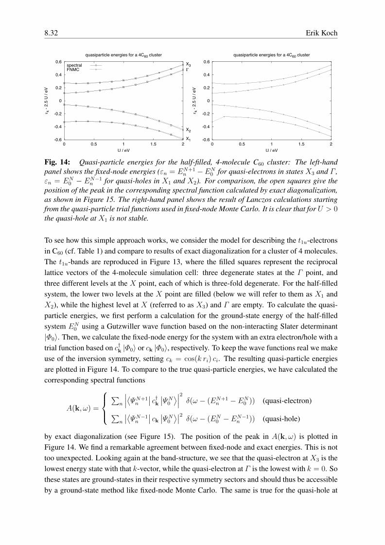
8.32 Erik Koch

-0.6

-0.4

-0.2

0

0.2

0.4

0.6

0 0.5 1 1.5 2

¡ k -

2.5

U /

eV

U / eV

quasiparticle energies for a 4C60 cluster

X1

X2

KX3spectral

FNMC

-0.6

-0.4

-0.2

0

0.2

0.4

0.6

0 0.5 1 1.5 2

¡ k -

2.5

U /

eV

U / eV

quasiparticle energies for a 4C60 cluster

Fig. 14: Quasi-particle energies for the half-filled, 4-molecule C60 cluster: The left-handpanel shows the fixed-node energies (εn = EN+1

n −EN0 for quasi-electrons in states X3 and Γ ,

εn = EN0 − EN−1

n for quasi-holes in X1 and X2). For comparison, the open squares give theposition of the peak in the corresponding spectral function calculated by exact diagonalization,as shown in Figure 15. The right-hand panel shows the result of Lanczos calculations startingfrom the quasi-particle trial functions used in fixed-node Monte Carlo. It is clear that for U > 0the quasi-hole at X1 is not stable.

To see how this simple approach works, we consider the model for describing the t1u-electronsin C60 (cf. Table 1) and compare to results of exact diagonalization for a cluster of 4 molecules.The t1u-bands are reproduced in Figure 13, where the filled squares represent the reciprocallattice vectors of the 4-molecule simulation cell: three degenerate states at the Γ point, andthree different levels at the X point, each of which is three-fold degenerate. For the half-filledsystem, the lower two levels at the X point are filled (below we will refer to them as X1 andX2), while the highest level at X (referred to as X3) and Γ are empty. To calculate the quasi-particle energies, we first perform a calculation for the ground-state energy of the half-filledsystem EN

0 using a Gutzwiller wave function based on the non-interacting Slater determinant|Φ0〉. Then, we calculate the fixed-node energy for the system with an extra electron/hole with atrial function based on c†k |Φ0〉 or ck |Φ0〉, respectively. To keep the wave functions real we makeuse of the inversion symmetry, setting ck = cos(k ri) ci. The resulting quasi-particle energiesare plotted in Figure 14. To compare to the true quasi-particle energies, we have calculated thecorresponding spectral functions

A(k, ω) =

∑

n

∣∣∣⟨ΨN+1n

∣∣ c†k ∣∣ΨN0 ⟩∣∣∣2 δ(ω − (EN+1n − EN

0 )) (quasi-electron)∑n

∣∣⟨ΨN−1n

∣∣ ck ∣∣ΨN0 ⟩∣∣2 δ(ω − (EN0 − EN−1

n )) (quasi-hole)

by exact diagonalization (see Figure 15). The position of the peak in A(k, ω) is plotted inFigure 14. We find a remarkable agreement between fixed-node and exact energies. This is nottoo unexpected. Looking again at the band-structure, we see that the quasi-electron at X3 is thelowest energy state with that k-vector, while the quasi-electron at Γ is the lowest with k = 0. Sothese states are ground-states in their respective symmetry sectors and should thus be accessibleby a ground-state method like fixed-node Monte Carlo. The same is true for the quasi-hole at

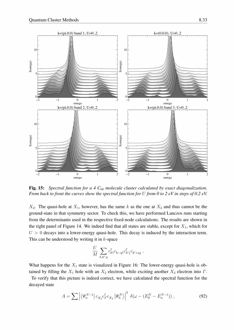
Quantum Cluster Methods 8.33

k=(pi,0,0) band 1, U=0..2

ï2 ï1 0 1 2omega

0

5

10

I(om

ega)

k=(0,0,0), U=0..2

ï2 ï1 0 1 2omega

0

5

10

I(om

ega)

k=(pi,0,0) band 2, U=0..2

ï2 ï1 0 1 2omega

0

5

10

I(om

ega)

k=(pi,0,0) band 3, U=0..2

ï2 ï1 0 1 2omega

0

5

10I(

omeg

a)

Fig. 15: Spectral function for a 4 C60 molecule cluster calculated by exact diagonalization.From back to front the curves show the spectral function for U from 0 to 2 eV in steps of 0.2 eV.

X2. The quasi-hole at X1, however, has the same k as the one at X2 and thus cannot be theground-state in that symmetry sector. To check this, we have performed Lanczos runs startingfrom the determinants used in the respective fixed-node calculations. The results are shown inthe right panel of Figure 14. We indeed find that all states are stable, except for X1, which forU > 0 decays into a lower-energy quasi-hole. This decay is induced by the interaction term.This can be understood by writing it in k-space

U

M

∑k,k′,q

c†k↑ck−q↑c†k′↓ck′+q↓ .

What happens for the X1 state is visualized in Figure 16: The lower-energy quasi-hole is ob-tained by filling the X1 hole with an X2 electron, while exciting another X2 electron into Γ .

To verify that this picture is indeed correct, we have calculated the spectral function for thedecayed state

A =∑∣∣∣⟨ΨN−1

n

∣∣ cX2c†Γ cX2

∣∣ΨN0 ⟩∣∣∣2 δ(ω − (EN0 − EN−1

n )) , (92)

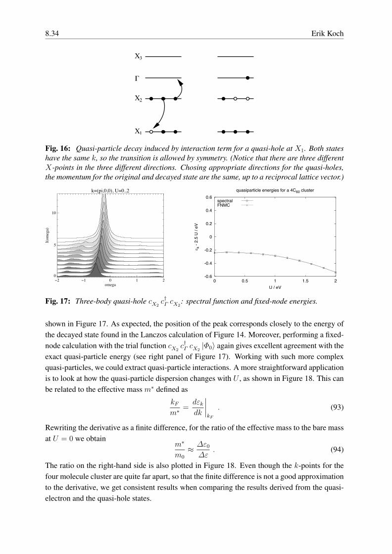
8.34 Erik Koch

X

2

1

3

X

X

K

Fig. 16: Quasi-particle decay induced by interaction term for a quasi-hole at X1. Both stateshave the same k, so the transition is allowed by symmetry. (Notice that there are three differentX-points in the three different directions. Chosing appropriate directions for the quasi-holes,the momentum for the original and decayed state are the same, up to a reciprocal lattice vector.)

k=(pi,0,0), U=0..2

ï2 ï1 0 1 2omega

0

5

10

I(om

ega)

-0.6

-0.4

-0.2

0

0.2

0.4

0.6

0 0.5 1 1.5 2

¡ k -

2.5

U /

eV

U / eV

quasiparticle energies for a 4C60 cluster

spectralFNMC

Fig. 17: Three-body quasi-hole cX2c†Γ cX2

: spectral function and fixed-node energies.

shown in Figure 17. As expected, the position of the peak corresponds closely to the energy ofthe decayed state found in the Lanczos calculation of Figure 14. Moreover, performing a fixed-node calculation with the trial function cX2

c†Γ cX2|Φ0〉 again gives excellent agreement with the

exact quasi-particle energy (see right panel of Figure 17). Working with such more complexquasi-particles, we could extract quasi-particle interactions. A more straightforward applicationis to look at how the quasi-particle dispersion changes with U , as shown in Figure 18. This canbe related to the effective mass m∗ defined as

kFm∗

=dεkdk

∣∣∣∣kF

. (93)

Rewriting the derivative as a finite difference, for the ratio of the effective mass to the bare massat U = 0 we obtain

m∗

m0

≈ ∆ε0

∆ε. (94)

The ratio on the right-hand side is also plotted in Figure 18. Even though the k-points for thefour molecule cluster are quite far apart, so that the finite difference is not a good approximationto the derivative, we get consistent results when comparing the results derived from the quasi-electron and the quasi-hole states.

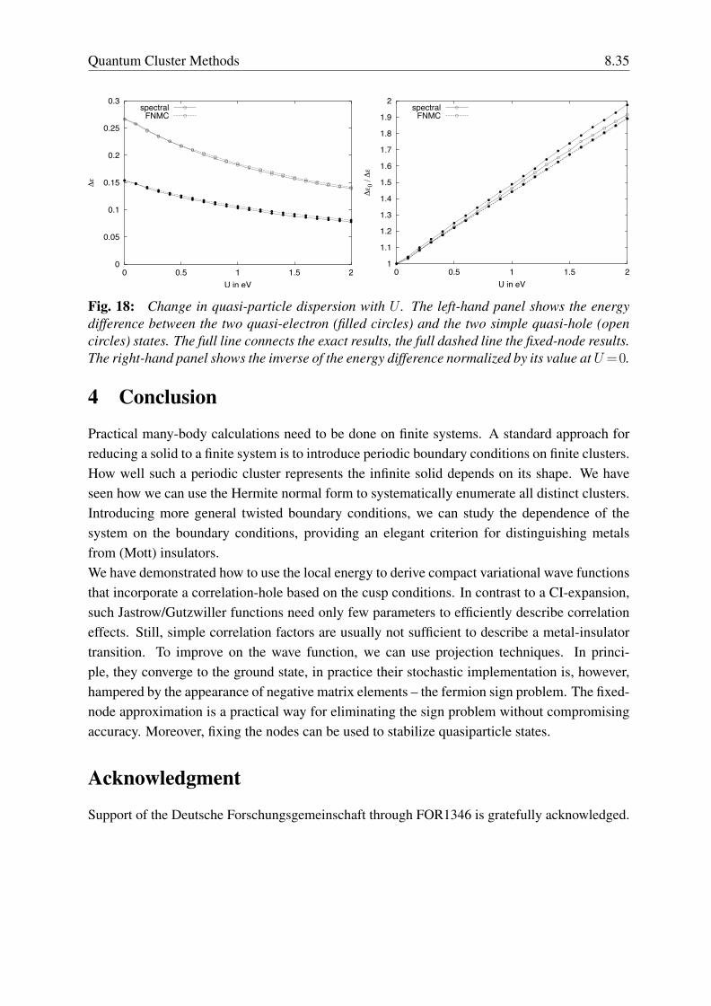
Quantum Cluster Methods 8.35

0

0.05

0.1

0.15

0.2

0.25

0.3

0 0.5 1 1.5 2

6¡

U in eV

spectralFNMC

1

1.1

1.2

1.3

1.4

1.5

1.6

1.7

1.8

1.9

2

0 0.5 1 1.5 2

6¡ 0

/ 6¡

U in eV

spectralFNMC

Fig. 18: Change in quasi-particle dispersion with U . The left-hand panel shows the energydifference between the two quasi-electron (filled circles) and the two simple quasi-hole (opencircles) states. The full line connects the exact results, the full dashed line the fixed-node results.The right-hand panel shows the inverse of the energy difference normalized by its value atU=0.

4 Conclusion

Practical many-body calculations need to be done on finite systems. A standard approach forreducing a solid to a finite system is to introduce periodic boundary conditions on finite clusters.How well such a periodic cluster represents the infinite solid depends on its shape. We haveseen how we can use the Hermite normal form to systematically enumerate all distinct clusters.Introducing more general twisted boundary conditions, we can study the dependence of thesystem on the boundary conditions, providing an elegant criterion for distinguishing metalsfrom (Mott) insulators.We have demonstrated how to use the local energy to derive compact variational wave functionsthat incorporate a correlation-hole based on the cusp conditions. In contrast to a CI-expansion,such Jastrow/Gutzwiller functions need only few parameters to efficiently describe correlationeffects. Still, simple correlation factors are usually not sufficient to describe a metal-insulatortransition. To improve on the wave function, we can use projection techniques. In princi-ple, they converge to the ground state, in practice their stochastic implementation is, however,hampered by the appearance of negative matrix elements – the fermion sign problem. The fixed-node approximation is a practical way for eliminating the sign problem without compromisingaccuracy. Moreover, fixing the nodes can be used to stabilize quasiparticle states.

Acknowledgment

Support of the Deutsche Forschungsgemeinschaft through FOR1346 is gratefully acknowledged.

8.36 Erik Koch

References

[1] E. Koch: Many-body states, in [33]

[2] A. Szabo and N.S. Ostlund: Modern Quantum Chemistry (Dover Publications, 1996)

[3] M. Born and T. von Karman, Physikal. Z. 13, 297 (1912)

[4] W.M.C. Foulkes, L. Mitas, R.J. Needs, and G. Rajagopal, Rev. Mod. Phys. 73, 33 (2001)

[5] E. Wigner, Phys. Rev. 46, 1002 (1934)

[6] W. Kohn, Phys. Rev. 133, A171 (1964)

[7] M. Newman: Integral Matrices (Academic Press, New York, 1972)

[8] H. Cohen: A Course in Computational Algebraic Number Theory(Springer, Heidelberg, 1993)

[9] D.D. Betts, H.Q. Lin, and J.S. Flynn, Can. J. Phys. 77, 353 (1999)

[10] H.J. Monkhorst and J.D. Pack, Phys. Rev. B 13, 5188 (1976)

[11] E. Koch: The Lanczos Method, in [31]

[12] T. Kato, Commun. Pure Appl. Math. 10, 151 (1957)

[13] B.L. Hammond, W.A. Lester, P.J. Reynolds:Monte Carlo Methods in Ab Initio Quantum Chemistry (World Scientific, 1994)

[14] R. Jastrow, Phys. Rev. 98, 1479 (1955)

[15] S. Fahy, X.W. Wang, and S.G. Louie, Phys. Rev. B 42, 3502 (1990)

[16] E. Pavarini and E. Koch: Introduction, in [31]

[17] M.C. Gutzwiller, Phys. Rev. 137, A1726 (1965)

[18] J. Bunemann: The Gutzwiller Density Functional Theory in [32]

[19] D.M. Ceperley, G.V. Chester, and M.H. Kalos, Phys. Rev. B 16, 3081 (1977)

[20] P. Horsch and T.A. Kaplan, J. Phys. C 16, L1203 (1983);H. Yokoyama and H. Shiba, J. Phys. Soc. Jpn. 56, 1490 (1987)

[21] E. Koch, O. Gunnarsson, and R.M. Martin, Phys. Rev. B 59, 15632 (1999)

[22] C. Umrigar, K. Wilson, and J. Wilkins, Phys. Rev. Lett. 60, 1719 (1988)

[23] E. Koch, O. Gunnarsson, and R.M. Martin, Phys. Rev. B 60, 15714 (1999)

Quantum Cluster Methods 8.37

[24] D. Vollhardt, Rev. Mod. Phys. 56, 99 (1984)

[25] W.F. Brinkman and T.M. Rice, Phys. Rev. B 2, 4302 (1970);T.M. Rice and W.F. Brinkman, in Critical Phenomena in Alloys, Magnets, andSuperconductors, ed. by R.E. Mills, E. Ascher, R. Jaffee (McGraw Hill, New York, 1971)

[26] W. Metzner and D. Vollhardt, Phys. Rev. Lett. 59, 121 (1987)and Phys. Rev. B 37, 7382 (1988)

[27] A.J. Millis and S.N. Coppersmith, Phys. Rev. B 43, 13770 (1991)

[28] N. Trivedi and D.M. Ceperley, Phys. Rev. B 40, 2737 (1989)

[29] D.F.B. ten Haaf, H.J.M. van Bemmel, J.M.J. van Leeuwen, and W. van Saarloos,Phys. Rev. Lett. 72, 2442 (1994) and D.F.B. ten Haaf, H.J.M van Bemmel,J.M.J. van Leeuwen, W. van Saarloos, and D.M. Ceperley, Phys. Rev. B 51, 13039 (1995)

[30] E. Koch, O. Gunnarsson, and R.M. Martin, Phys. Rev. Lett. 83, 620 (1999)

[31] E. Pavarini, E. Koch, D. Vollhardt, and A. Lichtenstein (eds.):The LDA+DMFT approacht to strongly correlated materialsReihe Modeling and Simulation, Vol. 1 (Forschungszentrum Julich, 2011)http://www.cond-mat.de/events/correl11

[32] E. Pavarini, E. Koch, F. Anders, and M. Jarrell (eds.):Correlated Electrons: From Models to MaterialsReihe Modeling and Simulation, Vol. 2 (Forschungszentrum Julich, 2012)http://www.cond-mat.de/events/correl12

[33] E. Pavarini, E. Koch, and U. Schollwock (eds.):Emergent Phenomena in Correlated matterReihe Modeling and Simulation, Vol. 3 (Forschungszentrum Julich, 2013)http://www.cond-mat.de/events/correl13