Quantitative Interprocedural Analysis · the effectiveness of our approach with two case studies. First, we show that our framework provides a sound approach (no false pos-itives)

Quantitative Interprocedural Analysis ∗

Krishnendu ChatterjeeAndreas Pavlogiannis

IST Austria (Institute of Science and TechnologyAustria) Klosterneuburg, Austria

{krish.chat, pavlogiannis}@ist.ac.at

Yaron VelnerTel Aviv University, [email protected]

AbstractWe consider the quantitative analysis problem for interprocedu-ral control-flow graphs (ICFGs). The input consists of an ICFG ,a positive weight function that assigns every transition a positiveinteger-valued number, and a labelling of the transitions (events) asgood, bad, and neutral events. The weight function assigns to eachtransition a numerical value that represents a measure of how goodor bad an event is. The quantitative analysis problem asks whetherthere is a run of the ICFG where the ratio of the sum of the numer-ical weights of good events versus the sum of weights of bad eventsin the long-run is at least a given threshold (or equivalently, to com-pute the maximal ratio among all valid paths in the ICFG). Thequantitative analysis problem for ICFGs can be solved in polyno-mial time, and we present an efficient and practical algorithm forthe problem. We show that several problems relevant for static pro-gram analysis, such as estimating the worst-case execution time ofa program or the average energy consumption of a mobile applica-tion, can be modeled in our framework. We have implemented ouralgorithm as a tool in the Java Soot framework. We demonstratethe effectiveness of our approach with two case studies. First, weshow that our framework provides a sound approach (no false pos-itives) for the analysis of inefficiently-used containers. Second, weshow that our approach can also be used for static profiling of pro-grams which reasons about methods that are frequently invoked.Our experimental results show that our tool scales to relatively largebenchmarks, and discovers relevant and useful information that canbe used to optimize performance of the programs.

Categories and Subject Descriptors D.3.4 [Programming Lan-guages]: Processors—Optimization; F.3.2 [Logics and Meaningsof Programs]: Semantics of Programming Langugages—ProgramAnalysis

General Terms Algorithms, Languages, Performance

Keywords Interprocedural analysis, Quantitative objectives,Mean-payoff and ratio objectives, Memory bloat, Static profiling.

∗ This work has been supported by the Austrian Science Foundation (FWF)under the NFN RiSE (S11405-07), FWF Grant P23499-N23, ERC Startgrant (279307: Graph Games), ERC grant 321174-VSSC, Israel ScienceFoundation grant 652/11, and Microsoft faculty fellows award.

Permission to make digital or hard copies of all or part of this work for personal orclassroom use is granted without fee provided that copies are not made or distributedfor profit or commercial advantage and that copies bear this notice and the full citationon the first page. Copyrights for components of this work owned by others than theauthor(s) must be honored. Abstracting with credit is permitted. To copy otherwise, orrepublish, to post on servers or to redistribute to lists, requires prior specific permissionand/or a fee. Request permissions from [email protected] ’15, January 15–17, 2015, Mumbai, India.Copyright is held by the owner/author(s). Publication rights licensed to ACM.ACM 978-1-4503-3300-9/15/01. . . $15.00.http://dx.doi.org/10.1145/2676726.2676968

1. IntroductionStatic and interprocedural analysis. Static analysis techniquesprovide ways to obtain information about programs without actu-ally running them on specific inputs. Static analysis explores theprogram behavior for all possible inputs and all possible execu-tions. For non-trivial programs, it is impossible explore all the pos-sibilities, and hence static analysis uses approximations (abstractinterpretations) to account for all the possibilities [16]. Static anal-ysis algorithms generally operate on the interprocedural control-flow graphs (for brevity ICFGs). An ICFG consists of a collectionof control-flow graphs (CFGs), one for each procedure of the pro-gram. The CFG of each procedure has a unique entry node anda unique exit node, and other nodes represent statements of theprogram and conditions (in other words, basic blocks of the pro-gram). In addition, there are call and return nodes for each pro-cedure which represent invoking of procedures and return fromprocedures. Call-transitions connect call nodes to entry nodes; andreturn-transitions connect exit nodes to return nodes. Algorithmicanalysis of ICFGs provides the mathematical framework for staticanalysis of programs. Interprocedural analysis with objectives suchas reachability, set-based information, etc have been deeply studiedin the literature [10, 24, 29, 31–33].

Quantitative objectives. A qualitative (or Boolean) objective as-signs to every run of a program a Boolean value (accept or reject). Aquantitative objective assigns to every run of a program a real valuethat represents a quality measure of the run. The analysis of pro-grams with quantitative objectives is gaining huge prominence dueto embedded systems with requirements on resource consumption,promptness of responses, performance analysis etc. Quantitativeobjectives have been proposed in several applications such as forworst-case execution time (see [41] for survey), power consump-tion [37], prediction of cache behavior for timing analysis [20],performance measures [5, 13, 21], to name a few. Another impor-tant feature of quantitative objectives is that they are very well-suited for anytime algorithms [8] (where anytime algorithms gen-erate imprecise answers quickly, and proceed to construct progres-sively better approximate solutions with refinements) (for a moreelaborate discussion see [12]).

Mean-payoff and ratio objectives. One of the most well-studiedand mathematically elegant quantitative objectives is the mean-payoff objective, where a rational-valued weight is associated withevery transition and the goal is to ensure that the long-run averageof the weights along a run is at least a given threshold [3, 19, 46].For example, consider a weight function that assigns to everytransition the resource (such as power) consumption, then themean-payoff objective measures the average resource consumptionalong a run. Along with ICFGs with mean-payoff objectives, wealso consider ratio objectives. For ratio objectives, the transitions(events) of the ICFGs are labelled as good, bad, or neutral events,and a positive weight function assigns a positive integer-valued

weight to every transition, and the weight function represents howgood or bad an event is. The quantitative analysis problem asks ifthere is a run of the program such that the ratio of the sum of theweights of the good events versus the weights of the bad events inthe long-run is at least a given threshold. For example, consider aweight function that assigns weight 1 to each transition, and a la-beling of events as follows: whenever a request is made is a badevent, whenever a request is pending is a good event, and wheneverno request is pending is a neutral event. The ratio objective assignsthe long-run average time between requests and the correspondinggrant per request for a run, and measures timeliness of responses torequests. Finite-state systems (or intraprocedural finite-state pro-grams) with mean-payoff objectives have been studied in the lit-erature in [19, 21, 26, 46] for performance modeling, and morerecently applied in synthesis of reactive systems with quality guar-antee [5] and robustness [6], reliability requirements and resourcebounds of reactive systems [9, 13, 17].Interprocedural quantitative analysis. Quantitative objectivessuch as mean-payoff and ratio objectives provide the appropriateframework to express several important system properties such asresource consumption and timeliness. While finite-state systemswith mean-payoff objectives have been studied in the literature,the static analysis of ICFGs with mean-payoff and ratio objectiveshas largely been ignored. An interprocedural analysis is precise ifit provides the meet-over-all-valid-paths solution (a path is valid ifit respects the fact that when a procedure finishes it returns to thesite of the most recent call). In the quantitative setting, the problemcorresponds to finding the maximal value over all valid paths and toproduce a witness (symbolic) path for that value. In this work, weconsider precise interprocedural quantitative analysis for ICFGswith mean-payoff and ratio objectives.Our contributions. In this work we present a flexible and generalmodelling framework for quantitative analysis and show how it canbe used to reason about quantitative properties of programs andabout potential optimizations in the program. We present an effi-cient polynomial-time algorithm for precise interprocedural quan-titative analysis, which is implemented as a tool. We demonstratethe efficiency of the algorithm with two case studies, and show thatour approach scales to programs with thousands of methods.1. (Theoretical modeling). We show that ICFGs with mean-

payoff and ratio objectives provide a robust framework that nat-urally captures a wide variety of static program analysis opti-mization and reasoning problems.(a) (Detecting container usage). An exceedingly important

problem for performance analysis is detection of runtimebloat that significantly degrades the performance and scal-ability of programs [27, 45]. A common source of bloat isinefficient use of containers [45]. We show that the prob-lem of detecting usage of containers can be modeled asICFGs with ratio objectives. A good use of a container cor-responds to a good event and no use of the container is a badevent, and a misuse is represented as a low ratio of good vsbad events. Hence the container usage problem is naturallymodeled as ratio analysis of ICFGs. While the problem ofdetecting container usage was already considered in [45],our different approach has the following benefits (see Sec-tion 5.2 for a comparison). First, our approach can handlerecursion ([45] does not handle recursion). Second, our ap-proach is sound, and does not yield false positives. Third,the approach of [45] ignored DELETE operations and we areable to take into consideration both ADD and DELETE oper-ations (thus provide a more refined analysis). Moreover, ouralgorithmic approach for analysis of ICFGs is polynomial,whereas the algorithmic approach of [45] in the worst casecan be exponential.

(b) (Static profiling of programs). We use our framework tomodel a conceptually new way for static profiling of pro-

grams for performance analysis. A line in the code (or acode segment) is referred as hot if there exists a run of theprogram where the line of code is frequently executed. Forexample, a function is referred as hot if there exists a runof the program where the function is frequently invoked,i.e., the frequency of calls to the function among all func-tion calls is at least a given threshold. Again this problem isnaturally modeled as ratio problem for ICFGs, and our ap-proach statically detects methods that are more frequentlyinvoked. Optimization of frequently executed code wouldnaturally lead to performance improvements and reasoningabout hot spots in the code can assist the complier to applyoptimization such as function inlining and loop unrolling(see Subsection 3.2 for more details).

(c) (Other applications). We show the generality of our frame-work by demonstrating that it provides an appropriateframework for theoretical modeling of diverse applicationssuch as interprocedural worst-case execution time analysis,evaluating speedup in parallel computation, and interproce-dural average energy consumption analysis.

2. (Algorithmic analysis). The quantitative analysis of ICFGswith mean-payoff objectives can be achieved in polynomialtime by a reduction to pushdown systems with mean-payoff ob-jectives (which can be solved in polynomial time [14]). How-ever, the resulting algorithm in the worst case has time complex-ity that is a polynomial of degree thirteen and space complexitythat is a polynomial of degree six (which is prohibitive in prac-tice). We exploit the special theoretical properties of ICFGsin order to improve the theoretical upper bound and get analgorithm that in the worst case runs in cubic time and withquadratic space complexity. In addition, we exploit the prop-erties of real-world programs and introduce optimizations thatgive a practical algorithm that is much faster than the theoreticalupper bound when the relevant parameters (the total number ofentry, exit, call, and returns nodes) are small, which is typicalin most applications. Finally we present a linear reduction ofthe quantitative analysis problem with ratio objectives to mean-payoff objectives.

3. (Tool and experimental results). We have implemented our al-gorithm and developed a tool in the Java Soot framework [38].We show through two case studies that our approach scales torelatively large programs from well-known benchmarks. Thedetails of the case studies are as follows:(a) (Detecting container usage). Our experimental results show

that our tool scales to relatively large benchmarks (DaCapo2009 [4]), and discover relevant and useful information thatcan be used to optimize performance of the programs. Ourtool could analyze all containers in several benchmarks (likemuffin) whereas [45] could analyze them partially (in muf-fin only half of the containers were analyzed in [45] — be-fore the predefined time bound was exceeded). Our soundapproach allows us to avoid false reports (that were reportedby [45]) and our simple mathematical modelling even al-lows us to report misuses that were not reported by [45].

(b) (Static profiling of programs). We run an analysis to detecthot methods for various thresholds. Our experimental re-sults on the benchmarks report only a small fraction of thefunctions as hot for high threshold values, and thus give use-ful information about potential functions to be optimized forperformance gain. In addition we perform a dynamic profil-ing and mark the top 5% of the most frequently invokedfunctions as hot. Our experiments show a significant corre-lation between the results of the static and dynamic analysis.In addition, we show that the sensitivity and specificity ofthe static classification can be controlled by considering dif-ferent thresholds, where lower thresholds increase the sen-sitivity and higher thresholds increase the specificity. We in-

vestigate the trade-off curve (ROC curve) and demonstratethe prediction power of our approach.

Thus we show that several conceptually different problems re-lated to program optimizations are naturally modeled in ourframework, and demonstrate that we present a flexible andgeneric framework for quantitative analysis of programs. More-over, our case studies show that our tool scales to benchmarkswith real-world programs.

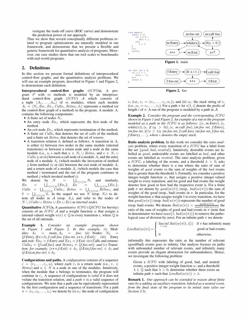
2. DefinitionsIn this section we present formal definitions of interproceduralcontrol-flow graphs, and the quantitative analysis problems. Wewill use an example program, described in Figure 1 and Figure 2,to demonstrate each definition.Interprocedural control-flow graphs (ICFGs). A pro-gram P with m methods is modeled by an interproce-dural control-flow graph (ICFG) A which consists ofa tuple ⟨A1, . . . , Am⟩ of m modules, where each moduleAi = ⟨Ni,Eni,Ex i,Callsi,Retnsi, δi⟩ represents a method (orthe control-flow graph of a method) in the program. A module Ai

contains the following components:• A finite set of nodes Ni.• An entry node Eni, which represents the first node of the

method.• An exit node Ex i, which represents termination of the method.• A finite set Callsi that denotes the set of calls of the method,

and a finite set Retns i that denotes the set of returns.• A transition relation δi defined as follows: A transition in Ai

is either (i) between two nodes in the same module (internaltransitions) or between a return node and a node in the samemodule (i.e., u, v such that u ∈ Ni ∪ Retns i and v ∈ Ni ∪Callsi); or (ii) between a call node of a module Ai and the entrynode of a module Aj (which models the invocation of methodj from method i); or (iii) between the exit node of module Ai

and a return node of a module Aj (which models the case thatmethod i terminated and the run of the program continues inmethod j which invoked method i).

We denote by N =⋃

1≤i≤m Ni and similarly,En =

⋃1≤i≤m{Eni}; Ex =

⋃1≤i≤m{Ex i};

Calls =⋃

1≤i≤m Callsi; Retns =⋃

1≤i≤m Retnsi; andδ =

⋃1≤i≤m δi. In the sequel we use N (resp. Ni) to de-

note all nodes in A (resp. Ai), and refer to the nodes ofN \ (Calls ∪ Retns ∪ En ∪ Ex) as internal nodes.Quantitative ICFGs. A quantitative ICFG (QICFG for brevity)consists of an ICFG A and a weight function w that assigns arational-valued weight w(e) ∈ Q to every transition e, where Q isthe set of all rationals.

Example 1. Consider an example program shownin Figure 1 and Figure 2. In this example, (i) Mod-ules: A1 = main, A2 = foo; (ii) Nodes: N2 ={f:Entry, if(x>1), f:call foo, f:foo ret, x++, f:Exit}; (iii) Entryand exit: En2 = f:Entry and Ex 2 = f:Exit; (iv) Calls and returns:Calls2 = {f:call foo} and Retns2 = {f:foo ret}; and (v) Transi-tion: for example, (x++,f:Exit) ∈ δ2, (f:Exit,f:foo ret) ∈ δ2 and(f:Exit,m:foo ret) ∈ δ2.

Configurations and paths. A configuration consists of a sequencec = (r1, . . . , rj , u), where each ri is a return node (i.e., ri ∈Retns) and u ∈ N is a node in one of the modules. Intuitively,when the module that u belongs to terminates, the program willcontinue in rj . A sequence of configurations is valid if it does notviolate the transition relation, and a path π is a valid sequence ofconfigurations. We note that a path can be equivalently representedby the first configuration and a sequence of transitions. For a pathπ = ⟨c1, c2, . . . , cℓ⟩ we denote by (i) ni: the node of configuration

v o i d main (){wh i l e ( x ){

i f ( y > 0 )f o o ( x ) ;

e l s ez = 7 ;

}z ++;r e t u r n ;

}

m:Entry while(x)

z++

if(y > 0 )

m:Exit

m:foo ret m:call foo

z=7

Figure 1. main

i n t f o o ( i n t x ){i f ( x > 1 )

f o o ( x − 1 ) ;x ++;r e t u r n x ;

}

f:Entry if( x>1 ) f:call foo

f:foo ret x++ f:Exit

Figure 2. foo

ci (i.e., ci = (r1, . . . , rj , ni)), and (ii) αi: the stack string of ci(i.e., αi = r1, . . . , rj). For a path π let π[1, i] denote the prefix oflength i of π. A run of the program is modeled by a path in A.

Example 2. Consider the program and the corresponding ICFGshown in Figure 1 and Figure 2. An example of a run in the programmodeled as a path in the ICFG is as follows: ⟨(ϵ, m:Entry), (ϵ,while(x)), (ϵ, if (y > 0)), (ϵ, m:call foo), (m:foo ret, f:Entry),(m:foo ret, if (x > 1)), (m:foo ret, f:call foo), (m:foo ret, f:foo ret,f:Entry), . . . ⟩, where ϵ denotes the empty stack.

Ratio analysis problem. In this work we consider the ratio anal-ysis problem, where every transition of a ICFG has a label fromthe set {good , bad ,neutral}. Intuitively, desirable events are la-belled as good , undesirable events are labelled as bad , and otherevents are labelled as neutral . The ratio analysis problem, givena ICFG , a labeling of the events, and a threshold λ > 0, asksto determine whether there is a run where the ratio of sum ofweights of good events vs the sum of weights of the bad eventsthat is greater than the threshold λ. Formally, we consider a positiveinteger-weight function w, that assigns a positive integer-valuedweight to every transition, and for good and bad events the weightdenotes how good or how bad the respective event is. For a finitepath π we denote by good(w(π)) (resp., bad(w(π))) the sum ofweights of the good (resp., bad) events in π. In particular, for theweight function w that assigns weight 1 to every transition, we havethat good(w(π)) (resp. bad(w(π))) represents the number of good(resp. bad) events. We denote Rat(w(π)) = good(w(π))

max{1,bad(w(π))} theratio of the sum of weights of good and bad events in π (note thatin denominator we have max{1, bad(w(π))} to remove the patho-logical case of division by zero). For an infinite path π we denote

LimRat(w(π))=

⎧⎪⎨

⎪⎩

lim infi→∞

Rat(w(π[1, i])) if π has infinitely manygood or bad events;

0 otherwise;

informally this represents the ratio as the number of relevant(good/bad) events goes to infinity. Our analysis focuses on pathswith unbounded number of relevant events, and infinitely manyevents provide an elegant abstraction for unboundedness. Hence,we investigate the following problem:

Given a ICFG with labeling of good, bad, and neutralevents, a positive integer weight function w, and a thresholdλ ∈ Q such that λ > 0, determine whether there exists aninfinite path π such that LimRat(w(π)) > λ.

Remark 1. Our approach can be extended to reason about finiteruns by a adding an auxiliary transition, labeled as a neutral event,from the final state of the program to its initial state (also seeSection 3.3).

Mean-payoff analysis problem. In the mean-payoff analysis prob-lem we consider a QICFG with a rational-valued weight functionw. For a finite path π in a QICFG we denote by w(π) the totalweight of the path (i.e., the sum of the weights of the transitionsin π), and by Avg(w(π)) = w(π)

|π| the average of the weights,where |π| denotes the length of π. For an infinite path π, we de-note LimAvg(w(π)) = lim infi→∞ Avg(w(π[1, i])). The mean-payoff analysis problem asks whether there exists an infinite path πsuch that LimAvg(w(π)) > 0. In Section 4 we show how the ratioanalysis problem of ICFGs reduces to the mean-payoff analysisproblem of QICFGs.Assigning context-dependent and path-dependent weights. Inour model the numerical weights are assigned to every transition ofa ICFG . First, note that since we consider weight functions as aninput and allow all weight functions, the weights could be assignedin a dependent way. Second, in general, we can have an ICFG ,and a finite-state deterministic automaton (such as a deterministicmean-payoff automaton [13]) that assigns weights. The determin-istic automaton can assign weights depending on different contexts(or call strings) of invocations, or even independent of the contextbut dependent on the past few transitions (i.e., path-dependent), i.e.,the automaton has the stack alphabet and transition of the ICFG asinput alphabet and assigns weights depending on the current stateof the automaton and an input letter. We call such a weight functionregular weight function. Given a regular weight function specifiedby an automaton A and an ICFG we can obtain a ICFG (that rep-resents the path-dependent weights) by taking their synchronousproduct, and hence we will focus on ICFGs for algorithmic anal-ysis. The regular weight function can also be an abstraction of thereal weight function, e.g., the regular weight function is an over-approximation if the weights that it assigns to the good (resp. bad)events are higher (resp. lower) than the real weights. If the origi-nal weight function is bounded, then an over-approximation with aregular weight function can be obtained (which can be refined to bemore precise by allowing more states in the automaton of the reg-ular weight function). Note that the new ICFG which is obtainedfrom an ICFG and automaton A has a blowup in the number ofstates of A, and thus there is a tradeoff between the precision of Aand the size of the new ICFG constructed.

3. Applications: Theoretical ModelingIn this section we show that many diverse problems for staticanalysis can be reduced to ratio analysis of ICFGs. We will presentexperimental results (in Section 5) for the problems described inSection 3.1 and Section 3.2.

3.1 Container analysisThe inefficient use of containers is the cause of many performanceissues in Java. An excellent exposition of the problem with sev-eral practical motivations is presented in [45]. The importance ofaccurate identification of misuse of containers that minimizes (andideally eliminates) the number of false warnings was emphasizedin [45] and much effort was spent to avoid false warnings for real-world programs. We show that the ratio analysis for ICFGs pro-vides a mathematically sound approach for the identification of in-efficient use of containers.Two misuses. We aim to capture two common misuses of contain-ers following the definitions in [45]. The first inefficient use is anunderutilized container that always holds very few number of ele-ments. The cause of inefficiency is two-fold: (i) a container is typi-cally created with a default number of slots, and much more mem-ory is allocated than needed; and (ii) the functionality that is asso-ciated with the container is typically not specialized to the case thatit has only very few elements. The second inefficiency is caused byoverpopulated containers that are looked up rarely, though poten-tially they can have many elements. This causes a memory waste

and performance penalty for every lookup. Thus we consider thefollowing two cases of misuse:1. A container is underutilized if there exists a constant bound on

the number of elements that it holds for all runs of the program.2. For a threshold λ, a container is overpopulated if for all runs of

the program the ratio of GET vs ADD operations is less than λ.We note that our approach is demand-driven (where users canspecify to check the misuse of a specific container).

Modeling. The modeling of programs as ICFGs is standard. Wedescribe how the weight function and the ratio analysis problem canmodel the problem of detecting misuses. We abstract the differentcontainer operations into GET, ADD, and DELETE operations. Forthis purpose we require the user to annotate the relevant classmethods by GET, ADD, or DELETE; and by a weight function thatcorresponds to the number of GET, ADD, or DELETE operationsthat the method does (typically this number is 1). For example,in the class HashSet, the add method is annotated by ADD, thecontains method is annotated by GET and the remove operationis annotated by DELETE. The clear operation which removes allelements from the set is annotated by DELETE but with a largeweight (if clear appears in a loop, it dominates the add operationsof the loop). We note that the annotation can be automated with theapproach that is described in [45].1. When detecting underutilized containers we define ADD opera-

tions as good events and DELETE operations as bad events, andcheck for threshold 1. Note that the relevant threshold is 1: ifthe (long-run) ratio of ADD vs DELETE is not greater than 1,then the total number of elements in the container is boundedby a constant.

2. When detecting overpopulated containers we define GET oper-ations as good events and ADD operations as bad events, andcheck for the given threshold λ.

In addition, since we wish to analyze heap objects, the allocationof the container is a bad event with a large weight (i.e., similareffect as of clear); see Example 3. The container is misused iffthe answer to the ratio analysis problem is NO (note that in theproblem description for container analysis we have quantificationover all paths and for ratio analysis of ICFGs the quantificationis existential). The detection is demand-driven and done for anallocated container c.

Details of modeling. Intuitively, a transition in the call graph is goodif it invokes a functionality that is annotated by a good operation(i.e., ADD operation for the underutilized analysis and GET opera-tion for the overpopulated analysis) and the object that invokes theoperation points to container c, and it is bad if the invoked operationis annotated as bad. Formally, for a given allocated container c: Ifat a certain line a variable t that may point to c invokes a good func-tionality, then we denote the transition as good. If t must point to cand invokes a bad functionality, then we denote it as a bad events.All other transitions are neutral. Note that our modeling is conser-vative. The misuse is detected for the container c if all runs of theprogram have a ratio of good vs bad events that is below the thresh-old (in other words, the container is not misused if there exists apath where the ratio of good vs bad events is above the threshold,and this exactly corresponds to the ratio analysis of ICFGs).

Example 3. We illustrate some important aspects of the containeranalysis problem with an example. Consider the program shown inFigure 3. We consider the containers that are allocated in line 9and in line 20 and analyze them for underutilization. There existruns that go through line 14 and properly use the container that isallocated in line 9, since qux method can add unbounded numberof elements to the hash table (due to its recursive call). However,the container in line 20 is underutilized, since in every run thenumber of elements is bounded by 2. However, note that if theDELETE operation is not handled, then the container is reportedas properly used. We note that since we assign large weights to

1 v o i d qux ( H a s h t a b l e h , i n t x ){2 h . p u t ( x , x / 2 ) ;3 i f ( x > 0 ){4 qux ( h , x / 2 ) ;5 }6 }78 H a s h t a b l e b ar ( i n t x ){9 r e t u r n new H a s h t a b l e ( x∗x ) ;

10 }

12 v o i d f o o ( i n t x ){13 i f ( x % 2){14 H a s h t a b l e h1 = b ar ( x ) ;15 qux ( h1 , x ) ;16 }17 e l s e18 {19 f o r ( i n t y = 0 ; y < x ; y++ ){20 H a s h t a b l e h2 = new H a s h t a b l e ( y ) ;21 h2 . p u t ( y , x ) ;22 f o r ( i n t z = 0 ; z < y ; z++ )23 {24 h2 . p u t ( z , y ) ;25 . . .26 h2 . remove ( z ) ;27 }28 }29 }30 }

Figure 3. An example for underutilized container analysis.

the allocation of the container, this prevents the analysis fromreporting that h2 properly uses the container that is allocated inline 20. In summary, the example illustrates the following importantfeatures: (1) the proper usage of the container should be tested alsooutside of its allocation site1 (as opposed to the approach of [45]);(2) sometimes the proper usage of a container is due to recursion;and (3) handling DELETE operations appropriately increases theprecision of analysis. While these important features are illustratedwith the toy example, such behaviors were also manifested in theprograms of the benchmarks (see Subsection 5.2 for details).

Soundness. Our ratio analysis approach for ICFGs is both soundand complete (with respect to the weighted abstracted ICFG).Since we use a conservative approach for assigning bad and goodevents, the ICFG we obtain for the misuse analysis of containersis sound and we get the following result.

Theorem 1. (SOUNDNESS). The underutilized and overpopulatedcontainer analysis through the ratio analysis problem on ICFGsis sound (do not report false positives, i.e., any reported misusedcontainer is truly misused).

Remark 2. We remark about the significance of the soundness ofour approach.• The soundness criteria is a very important and desirable feature

for container analysis (for details see [43, 45]), because areported misused container needs to be analyzed manually andincurs a substantial effort for optimization. Hence as arguedin [43, 45], spurious warnings (false positive) of misuse mustbe minimized. In our approach, a misuse is reported iff in everyrun a misuse is detected, and with a sound (over approximation)annotation of the weights our approach is sound.

• The soundness of our approach is with respect to a sound (overapproximation) annotation of the ADD , DELETE and GEToperations. In addition, for a given ICFG , our ratio analysisis precise (i.e.. both sound and complete), hence, our containeranalysis is sound.

3.2 Static profilingFinding the most frequently executed lines in the code can helpthe programmer to identify the critical parts of the program andfocus on the optimization of these parts. It can also assist thecompiler (e.g., a C compiler) to decide whether it should applycertain optimizations such as function inlining (replacing a functioncall by the body of the called function) and loop unrolling (re-writethe loop as a repeated sequence of similar independent statements).These optimizations can reduce the running time of the program,but on the other hand, they increase the size of the (binary) code.Hence, knowing whether the function or loop is hot (frequently

1 E.g., an HashTable is allocated in bar function but the proper usage is doneoutside the allocation site, namely, after the termination of bar.

invoked) is important when considering the time vs. code sizetradeoff. In this subsection we present the model for profiling thefrequency of function calls (which allows finding hot functions),and we note that our profiling technique is generic and can be scaledto detect other hot spots in the code (e.g., hot loops).

Problem description. Given a program with several functions, afunction f is called λ-hot, if there exists a run (of unboundedlength) of the program where the frequency of calls to f (amongall function calls in the run) is at least λ. Formally, for a run,given a prefix of length i, let #f(i) denote the number of callsto f and #c(i) denote the number of function calls in the prefixof length i. The function is λ-hot if there exists a run such thatlim infi→∞

#f(i)#c(i) > λ.

Modeling. The modeling of programs as ICFGs is straightfor-ward. We describe the labeling of events and weight function inICFGs to determine if a function f is λ-hot. First we label call-transitions to f as good events and assign weight 1; then we labelall other call-transitions as bad events and assign them weight 1. Toensure that the number of calls to f also appear in the denomina-tor (in the total number of calls) we label transitions from the entrynode of f as bad events with weight 1. The function f is λ-hot iffthe answer to the ratio analysis problem with threshold λ is YES.

3.3 Estimating worst-case execution timeThe approach of [12] for estimating worst-case execution time(WCET) is also naturally captured by ratio analysis. While the in-traprocedural problem was considered in [12], our approach allowsthe more general interprocedural analysis. In this approach, we con-sider (as in [12]) that each program statement is assigned a cost thatcorresponds to its running time (e.g., number of CPU cycles).

Modeling. The modelling of WCET analysis of the program is asfollows: We add to the ICFG of the program a transition fromevery terminal node to the initial node, and every such transition isa bad event with weight 1. All the other transitions are good eventsand their weight is their cost (running time). The WCET of theprogram is at most N cycles if and only if the answer to the ratioanalysis problem with threshold N is NO.

3.4 Evaluating the speedup in a parallel computationThe speed of a parallel computing is limited by the time needed forthe sequential fraction of the program. For example, if a programruns for 10 minutes on a single processor core, and a certainpart of the program that takes 2 minutes to execute cannot beparallelized, then the minimum execution time cannot be less thantwo minutes (regardless of how many processors are devoted toa parallelized execution of this program). Hence, the speedup is atmost 5. Amdahl’s law [1] states that the theoretical speedup that canbe obtained by executing a given algorithm on a system capable ofexecuting n threads of execution is at most 1

B+ 1n (1−B)

, where B isthe fraction of the algorithm that is strictly serial. Our ratio analysistechnique can be used to (conservatively) estimate the value of Band thus to evaluate the outcome of Amdahl’s law.

Modeling. As in Section 3.3, we consider that the cost of everyprogram statement is given, and we add to the ICFG of the pro-gram a transition from every terminal node to the initial node, thistime as a neutral event with weight 0. All the transitions of the codethat cannot be parallelized are defined as good events, and the othertransitions are defined as bad events. We denote by P the fractionof the code that can be parallelized and by S the fraction of the codethat is strictly serial. The value of S

P is at most λ if and only if theanswer to the ratio analysis problem with threshold λ is NO. HenceB is bounded by 1

1+ 1λ

for which the answer to the ratio analysisproblem with threshold λ is NO.

3.5 Average energy consumptionIn the case of many consumer electronics devices, especially mo-bile phones, battery capacity is severely restricted due to constraintson size and weight of the device. This implies that managing energywell is paramount in such devices. Since most mobile applicationsare non-terminating (e.g., a web browser), the most important met-ric for measuring energy consumption is the average memory con-sumption per time unit [11], e.g., watts per second.Modeling. We consider that the running time and energy consump-tion of each statement in the application code is given (or is approx-imated). In our modeling we split each transition in the ICFG intotwo consecutive transitions, the first is a good event and the next isa bad event. The good event is assigned with a weight that corre-sponds to the energy consumption of the program statement and thebad event is assigned with a weight that corresponds to the runningtime of the statement. The average energy consumption of the ap-plication is at most λ if and only if the answer to the ratio analysisproblem is NO.

4. Algorithm for Quantitative Analysis ofQICFGs

In this section we present three results. The mean-payoff analysisproblem for QICFGs can be solved in polynomial time, this canbe derived from [14]. First, we present an algorithm that signifi-cantly improves the current theoretical bound for the problem forQICFGs. Second, we present an efficient algorithm that in mostpractical cases is much faster as compared to the theoretical upperbound. Finally, we present a linear reduction of the ratio analysisproblem to the mean-payoff analysis problem for QICFGs.

4.1 Improved algorithm for mean-payoff analysisIn this section we first discuss the basic polynomial-time algorithmfor mean-payoff analysis of QICFGs that can be obtained fromthe results on pushdown systems shown in [14]. Due to spaceconstraints the technical proofs are relegated to the supplementarymaterial.Results of [14] and reduction. The results of [14] show thatpushdown systems with mean-payoff objectives can be solved inpolynomial time. Given a pushdown system with state space Qand stack alphabet Γ, the polynomial-time algorithm of [14] canbe described as follows. The algorithm is iterative, and in eachiteration it constructs a finite graph of size O(|Q| · |Γ|2) and runs aBellman-Ford style algorithm on the finite graph from each vertex.The Bellman-Ford algorithm on the finite graph from all verticesin each iteration requires O(|Q|3 · |Γ|6) time and O(|Q|2 · |Γ|4)space. The number of iterations required is O(|Q|2 · |Γ|2). Thusthe time and space requirement of the algorithm are O(|Q|5 · |Γ|8)and O(|Q|2 · |Γ|4), respectively. A QICFG can be interpretedas a pushdown system where N corresponds to Q and Retnscorresponds to Γ.

Theorem 2. (BASIC ALGORITHM [14]). The mean-payoff analy-sis problem for QICFGs can be solved in O(|N |5 · |Retns |8) timeand O(|N |2 · |Retns |4) space, respectively.

Improved algorithm. We will present an improved polynomial-time algorithm for the mean-payoff analysis of QICFGs. Theimprovement relies on the following properties of QICFGs:1. The transitions of a module are independent of the stack of a

configuration, while in pushdown systems the transitions candepend on the top symbol of the stack. This enables to reducethe size of the finite graphs to be considered in every iteration.

2. Every call node has only one corresponding return node. There-fore, if a module A1 invokes a module A2, then the behavior ofA1 after the termination of A2 is independent of A2. This en-ables us to reduce the number of iterations to O(|Calls |).

To present the improved algorithm and its correctness formally, weneed a refined analysis and extensions of the results of [14]. Wefirst describe a key aspect and present an overview of the solution.

Remark 3. (Infinite-height lattice). Our algorithm will be an it-erative algorithm till some fixpoint is reached. However, for inter-procedural analysis with finite-height lattices, fixpoints are guaran-teed to exist. Unfortunately in our case for mean-payoff objectives,it is an infinite-height lattice. Thus a fixpoint is not guaranteed.For this reason the analysis for mean-payoff objectives is more in-volved, and this is even in the case of finite graphs. For example, forreachability objectives in finite graphs linear-time algorithms ex-ist, whereas for finite graphs with mean-payoff objectives the best-known algorithms (for over three decades) are quadratic [23].

Solution overview. In finite graphs the solution for the mean-payoff analysis is to check whether the graph has a cycle C suchthat the sum of weights of C is positive. If such a cycle exists, thena lasso path that leads to the cycle and then follows the cyclic pathforever has positive mean-payoff value. For QICFGs we show thatit is enough to find either a loop in the program such that the sumof weights of the loop is positive or a sequence of calls and returnswith positive total weight such that the last invoked module is thesame as the first invoked module. For this purpose we compute asummary function that finds the maximum weight (according to thesum of weights) path between every two statements of a method(i.e., between every two nodes of a module). The computation is anextension of the Bellman-Ford algorithm to QICFGs. We showthat it is enough to compute a summary function for QICFGswith a stack height that is bounded by some constant, and thenall that is left is to mark pairs of nodes such that the weight of amaximal weight path between them is unbounded. In finite graphsthe maximum weight between two vertices is unbounded only ifthe graph has a cycle with positive sum of weights (i.e., a pathwith positive total weight that can be pumped). For QICFGs itis also possible to pump special types of acyclic paths. We firstcharacterize these pumpable paths (up to Lemma 2). We then showhow to compute a bounded summary function (Lemma 3 and theparagraph that follows it and Example 5). Finally we show howto use the summary function to solve the mean-payoff analysisproblem. We start with the basic notions related to stack heightsand pumpable paths, and their properties which are crucial for thealgorithm.Stack heights. The configuration stack height of c =(r1, . . . , rj , u), denoted as SH(c), is j. For a finite path π =⟨(α1, n1), . . . , (αℓ, nℓ)⟩, the stack height of the path (denoted bySH(π)) is the maximal stack height of all the configurations inthe path. Formally SH(π) = max{|α1|, . . . , |αℓ|}. The addi-tional stack height of π is the additional height of the stack in thesegment of the path, i.e., the additional stack height ASH(π) isSH(π)−max(|α1|, |αℓ|).Pumpable pair of paths. Let π = ⟨c1t1t2 . . . ⟩ be a finite or infinitepath (where each ti is a transition in the QICFG). A pumpablepair of paths for π is a pair of non-empty sequences of transitions:(p1, p2) = (ti1ti1+1 . . . ti1+ℓ1 , ti2ti2+1 . . . ti2+ℓ2), for ℓ1, ℓ2 ≥0, i1 ≥ 0 and i2 > i1 + ℓ1 such that for every j ≥ 0 the pathπj(p1,p2)

obtained by pumping the pair p1 and p2 of paths j timeseach is a valid path, i.e., for every j ≥ 0 we have

πj(p1,p2)

= ⟨c1t1 . . . ti1−1(p1)jti1+ℓ1+1 . . . ti2−1(p2)

jti2+ℓ2+1 . . . ⟩

is a valid path. We illustrate the above definitions with the nextexample.

Example 4. Consider the program from Figure 1 and Figure 2 andthe corresponding ICFG . A possible path in the program is

m:Entry → while(x) → if(y>0) → m:call foo →f:Entry → if(x>1) → f:call foo → f:Entry → if(x>1) →

x++ → f:Exit → f:foo ret → x++ → f:Exit →m:foo ret→ while(x)

and we denote this path with π. Then ASH(π) = 2, and the pairof paths f:Entry → if(x>1) → f:call foo and f:foo ret → x++ →f:Exit is a pumpable pair of paths.

In the next lemmas we first show that every path with largeadditional stack has a pumpable pair of paths, and then establish theconnection of additional stack height and the existence of pumpablepair of paths with positive weights in Lemma 2. The key intuitionfor the proof of the next lemma is that a path with ASH(π) >|Calls|+ 1 must contain a recursive call that can be pumped.

Lemma 1. Let π be a finite path with ASH(π) = d > |Calls|+1.Then π has a pumpable pair of paths.

Lemma 2. Let c1, c2 be two configurations and j ∈ Z. Let d ∈ Nbe the minimal additional stack height of all paths between c1 andc2 with total weight at least j. If d > |Calls|+ 1, then there existsa path π∗ from c1 to c2 with additional stack height d that has apumpable pair (p1, p2) with w(p1) + w(p2) > 0.

Proof. Let us consider the set of paths Π between c1 and c2 withtotal weight at least j, and let Πmin be the subset of Π that hasminimal additional stack height. The proof is by induction on thelength of paths in Πmin. Consider a path π from Πmin that has theshortest length among all paths in Πmin. Since ASH(π) = d >|Calls| + 1, then by Lemma 1 it contains a pumpable pair. Let usconsider the path π1 obtained from π by pumping the pumpablepair zero times (i.e., the pumpable pair is removed). Since weremove a part of the path we have that ASH(π1) ≤ ASH(π).If w(π1) ≥ w(π), then we obtain a path π1 with weight atleast j, with either smaller additional stack height than π, or ofshorter length, contradicting that π is the shortest length minimaladditional stack height path with weight at least j. Hence we musthave w(π1) < w(π), and hence the pumpable pair has positiveweight. Now for an arbitrary path π in Πmin we obtain that it hasa pumpable pair. Either the pumpable pair has positive weight andwe are done, else removing the pumpable pair we obtain a shorterlength path of the same stack height, and the result follows byinductive hypothesis on the length of paths.

Our algorithm for the mean-payoff analysis problem is based ondetecting the existence of certain non-decreasing paths with posi-tive weight. The maximal weights of such non-decreasing pathsbetween node pairs are captured with the notion of a summaryfunction and bounded summary functions (with bounded additionalstack height). We now define them, and establish the lemma relatedto the number of bounded summary functions to be computed.Local minimum and non-decreasing paths. A configuration ci ina path π = ⟨c1, . . . , cℓ⟩ is a local minimum if the stack heightof ci is minimal in π, i.e., |αi| = min(|α1|, . . . , |αℓ|). A pathfrom configuration (α, n1) to (αβ, n2) is a non-decreasing α-path if (α, n1) is a local minimum. Note that if a sequence oftransitions is a non-decreasing α-path for some α ∈ Retns∗, thenthe same sequence of transitions is a non-decreasing γ-path forevery γ ∈ Retns∗. Hence, we say that π is a non-decreasing pathif there exists α ∈ Retns∗ such that π is a non-decreasing α-path.Summary function. Given the QICFG A and α ∈ Retns∗, wedefine a summary function sα :

⋃1≤ℓ≤m(Nℓ ×Nℓ) → {−∞} ∪

Z ∪ {ω} as:1. sα(n1, n2) = z ∈ Z iff the weight of the maximum weight

non-decreasing path from configuration (α, n1) to configura-tion (α, n2) is z.

2. sα(n1, n2) = ω iff for all j ∈ N there exists a non-decreasingpath from (α, n1) to (α, n2) with weight at least j.

3. sα(n1, n2) = −∞ iff there is no non-decreasing path from(α, n1) to (α, n2).

We note that for every α, β ∈ Retns∗ it holds that sα ≡ sβ .Hence, we consider only s ≡ sϵ (where ϵ is the empty stringand corresponds to empty stack). The computation of the summaryfunction is done by considering stack height bounded summaryfunctions defined below.Stack height bounded summary function. For everyd ∈ N, the stack height bounded summary functionsd :

⋃1≤ℓ≤m(Nℓ × Nℓ) → {−∞} ∪ Z ∪ {ω} is defined

as follows: (i) sd(n1, n2) = z ∈ Z iff the weight of the maximumweight non-decreasing path from (ϵ, n1) to (ϵ, n2) with additionalstack height at most d is z; (ii) sd(n1, n2) = ω iff for all j ∈ Nthere exists a non-decreasing path from (ϵ, n1) to (ϵ, n2) withweight at least j and additional stack height at most d; and(iii) sd(n1, n2) = −∞ iff there is no non-decreasing path withadditional stack height at most d from (ϵ, n1) to (ϵ, n2).

Facts of summary functions. We have the following facts: (i) forevery d ∈ N, we have sd+1 ≥ sd (monotonicity); and (ii) sd+1

is computable from sd and the QICFG . By the above facts weget that if sd ≡ sd+1, i.e., if a fix point is reached, then s ≡ sd.For interprocedural analysis with finite-height lattices, fix pointsare guaranteed to exist. Unfortunately in our case, the image of si isinfinite and moreover, it is an infinite-height lattice. Thus a fix pointis not guaranteed. The next lemma shows that we can compute allthe non-ω values of s with the bounded summary function.

Lemma 3. Let d = |Calls|+1. For all n1, n2 ∈ N , if s(n1, n2) ∈Z ∪ {−∞}, then s(n1, n2) = sd(n1, n2).

By Lemma 3 we get that if sd+1(n1, n2) > sd(n1, n2) (for d =|Calls|+1), then s(n1, n2) = ω. Hence, the summary function s isobtained by the fix point of the following computation: (i) Computesi+1 from si up to sd for d = |Calls| + 1; (ii) for i ≥ |Calls| +1, if si+1(n1, n2) > si(n1, n2), then set si+1(n1, n2) = ω;(iii) a fix point is reached after at most O(|Calls |) iterations (say jiterations), and then we set s ≡ sj . This establishes that we requireonly O(|Calls|) iterations as compared to O(|N |2 · |Retns |2)iterations. The number of returns and calls are the same and thuswe significantly improve the number of iterations required fromthe quartic worst-case bound to linear bound. We now describe thecomputation of every iteration to obtain si+1 from si.Computation of si+1 from si. We first compute a partial func-tion, namely, s′i+1 : En × Ex → {−∞,ω} ∪ Z that satisfiess′i+1(n1, n2) = si+1(n1, n2) for every n1 ∈ En and n2 ∈ Ex .We initialize s′0(n1, n2) = s0(n1, n2). For every module Aℓ weconstruct a finite graph Gi

ℓ by taking all the nodes and transitionsof Aℓ and by adding a transition between every call node and itscorresponding return node. For every transition between a pair ofnodes n1, n2 ∈ Nℓ \ (Callsℓ ∪ Retnsℓ) we assign the weight ac-cording to the original weight in A. For every transition between acall node that invokes module Ap and a corresponding return nodewe assign the weight s′i(Enp,Ex p). To compute s′i+1 for moduleAℓ we run one Bellman-Ford iteration over Gi

ℓ for source node Enℓ

and target node Ex ℓ. We observe the next two key properties of s′i:• For every iteration i, a module Aℓ, and pair of nodes n1, n2 ∈Nℓ we have that the weight of the maximum weight path be-tween n1 and n2 in Gi

ℓ is exactly si+1(n1, n2) (the proof is bya simple induction over i).

• If s′i+1 ≡ s′i, then si+1 ≡ si (follows from the first keyproperty).

Hence, to compute s we compute s′i+1 from s′i until we get s′i+1 ≡s′i, and then we compute all pairs maximum weight paths (e.g.,by the Floyd-Warshall algorithm) over every Gi

ℓ and get si+1

(and si+1 ≡ s). The Floyd-Warshall algorithm has a cubic timecomplexity and quadratic space complexity [15]. Therefore, thetime complexity for computing every iteration of si is O(

∑|Nℓ|2)

and the complexity of the last step is O(∑

|Nℓ|3). The space

complexity of the last step is O(max{|N1|, . . . , |Nm|}2), but tostore si we require O(

∑|Nℓ|2) space.

Summary graph. Given QICFG A with a summary func-tion s, we construct the summary graph Gr(A) = (V,E)of A with a weight function w : E → Z ∪ {ω} asfollows: (i) V = N \ (Ex ∪ Retns); and (ii) E =Einternal ∪ Ecalls where Einternal = {(n1, n2) | n1, n2 ∈Nℓ for some ℓ, and s(n1, n2) > −∞} contains the transitions inthe same module and Ecalls = {(n1, n2) | n1 ∈ Calls and n2 ∈En and n1 is a call to a module with entry node n2} contains thecall transitions. The weights of Einternal are according to the sum-mary function s and the weights of Ecalls are according to theweights of these transitions in A (i.e., according to w). A simplecycle in Gr(A) is a positive simple cycle iff one of the followingconditions hold: (i) the cycle contains an ω edge; or (ii) the sum ofthe weights of the cycles according to the weights of the summarygraph is positive. Lemma 4 shows the equivalence of the mean-payoff analysis problem and positive cycles in the summary graph.

Lemma 4. A QICFG A has a path π with LimAvg(w(π)) > 0iff the summary graph Gr(A) has a (reachable) positive cycle.

Proof. If Gr(A) does not contain a positive cycle, then it followsthat the weight of every non-decreasing path in A is bounded by theweight of the maximum weight path in Gr(A). Hence, for everyinfinite path π we get that every prefix of π is a non-decreasingpath from the initial configuration with bounded weight (sum ofweights bounded from above), and therefore LimAvg(w(π)) ≤ 0.Conversely, if Gr(A) has a positive cycle, then it follows that thereis a path π0π1 in Gr(A) such that π0 and π1 are non-decreasingpaths, π1 begins and ends in the same node (possibly at higherstack height) and w(π1) > 0. Hence, the path π0πω

1 is a validpath and satisfies LimAvg(w(π0πω

1 )) = w(π1)|π1|

> 0, whereπω1 = π1 · π1 · π1 . . . is the infinite concatenation of the finite

path π1. The desired result follows.

Algorithm and analysis. Algorithm 1 solves the mean-payoff anal-ysis problem for QICFGs. The computation of the summary func-tion requires O(|Calls|) computations of the partial summary func-tion s′i, which requires m runs of Bellman-Ford algorithm, each runover a graph of size |Nℓ| (hence, each run takes O(|Nℓ|2) time).In addition the computation requires m runs of all pairs maximumweight path (Floyd-Warshall) algorithm. Each run is over a graph ofsize O(|Nℓ|) (hence, each run takes O(|Nℓ|3) time and O(|Nℓ|2)space). Finally we detect positive cycles by running Bellman-Fordalgorithm once over the summary graph, which takes O(|N |2) timeand O(|N |) space. Thus we obtain the following result.

Theorem 3. (IMPROVED ALGORITHM). Algorithm 1solves the mean-payoff analysis problem for QICFGs inO((|Calls| · (

∑|Nℓ|2)

)+ (

∑|Nℓ|3) + |N |2

)time and

O(∑

|Nℓ|2) space.

Remark 4. Note that in the worst case the running time of Algo-rithm 1 is cubic and the space requirement is quadratic.

The next example is an illustration of a run of Algorithm 1.

Example 5. Consider the QICFG that consists of modules f andg (Figures 4 and 5) and the entry of f is the initial entry of theprogram. We now describe the run of Algorithm 1 over the QICFG .For simplicity, we denote the graph of f by F and the graph of g byG (and not by G1 and G2). Note that the number of call nodes is 3.

We first compute the summary function s′ and the first stepis to compute s′0. We have s′0(f:entry,f:exit) = −35, ands′0(g:entry,g:exit) = −25.

In order to compute s′1(f:entry,f:exit) we construct a graph F 0

from F by adding a transition from the node f:call g to the nodef:ret g with weight s′0(g:entry,g:exit) and find the maximum weight

Algorithm 1 Mean-payoff QICFG Analysis1: for ℓ← 1 to m do2: s′0(Enℓ,Ex ℓ) ← BELLMAN-FORD(Aℓ) {Compute s′0 by

running Bellman-Ford algorithm on Aℓ}3: end for4: i← 15: loop6: for ℓ← 1 to m do7: Construct Gi−1

ℓ according to s′i−1

8: s′i(Enℓ,Ex ℓ)← BELLMAN-FORD(Gi−1ℓ ) {Compute s′i

by running Bellman-Ford algorithm over Gi−1ℓ }

9: end for10: if s′i ≡ s′i−1 then11: break12: end if13: if i > |Calls|+ 1 then14: for ℓ← 1 to m do15: if s′i(Enℓ,Ex ℓ) > s′i−1(Enℓ,Ex ℓ) then16: s′i(Enℓ,Ex ℓ) = ω17: end if18: end for19: end if20: i← i+ 121: end loop22: s←FLOYD-WARSHALL(s′i)23: Construct Gr(A) from s24: BELLMAN-FORD(Gr(A)) {Run Bellman-Ford over Gr(A)}25: if Gr(A) has a positive cycle then26: return YES27: else28: return NO29: end if

f:call g f:g ret

f:entry f:v f:exit-30

-10-15-5

Figure 4. Module f

g:entry g:u1

g:call g g:ret g

g:u2 g:exit

g:call f g:ret f

-10-5

-1035

-5

-10

-10

Figure 5. Module g

f:call g

f:entry f:v-30

-15

g:entry g:u1

g:call g

g:u2

g:call f

-10

-5

ω

-100

0

0

Figure 6. Summary graph of f and g

path from f:entry to f:exit in F 0. We get s′1(f:entry,f:exit) = −35.In order to compute s′1(g:entry,g:exit) we construct a graph G0

from G by adding a transition from g:call g to g:ret g with weights′0(g:entry,g:exit) and a transition from g:call f to g:ret f withweight s′0(f:entry,f:exit) and find the maximum weight path fromg:entry to g:exit in G0. We get s′1(g:entry,g:exit) = −10.

Since s′1 = s′0, we continue to compute s′2. We construct F 1 andG1 in the same manner as we constructed F 0 and G0 (but takethe values of s′1 instead of s′0) and get s′2(f:entry,f:exit) = −35,s′2(g:entry,g:exit) = 5. For i = 3 we get s′3(f:entry,f:exit) = −35,s′3(g:entry,g:exit) = 20. For i = 4, s′4(f:entry,f:exit) = −35,s′4(g:entry,g:exit) = 35.

For i = 5 we get s′5(f:entry,f:exit) = −20 ands′5(g:entry,g:exit) = 50. Since i > |Calls| + 1 ands′5(f:entry,f:exit) > s′4(f:entry,f:exit) and s′5(g:entry,g:exit) >s′4(g:entry,g:exit) we assign assign s′5(f:entry,f:exit) = ω ands′5(g:entry,g:exit) = ω. In the sixth iteration we get a fix point(that is, s′6 ≡ s′5) and exit the loop block.

From F 5 and G5 we compute the summary function s.For example s(g:entry,g:u1) = ω and s(f:entry,f:v) = −30.Finally, we construct the summary graph (see Figure 6)and check whether a positive cycle exists. The cyclef:entry→f:v→f:call g→g:entry→g:u1→g:u2→g:call f→f:entrycontains an ω-edge and thus, it is a positive cycle. Hence algorithmreturns YES.

4.2 Efficient algorithm for mean-payoff analysisIn this section we further improve the algorithm for the mean-payoff analysis problem for QICFGs, and the improvement de-pends on the fact that typically the number of entry, exit, call, andreturns nodes is much smaller than the size of the QICFGs. For-mally, in most typical cases we have |Ex∪Retns∪Calls∪En| <<|N |. Let Xℓ = {Ex ℓ,Enℓ} ∪ Retnsℓ ∪ Callsℓ and X =

⋃ℓ Xℓ.

We present an improvement that enables us to construct the sum-mary function over graphs of size O(|Xℓ|) (instead of graphs ofsize O(|Nℓ|) of Section 4.1), and with at most O(|Calls |) iter-ations. Hence, the algorithm in most typical cases will be muchfaster and require much smaller space.Compact representation. The key idea for the improvement isto represent the modules in compact form. The compact form ofa module Aℓ, denoted by Comp(Aℓ), consists of the entry, exit,call, and returns node of Aℓ. There is transition between everynode in Comp(Aℓ), and the weight of each transition is the maxi-mum weight path between the nodes with additional stack height0 (and if there is no such path, then the weight is −∞). For-mally, Comp(Aℓ) = (V,E); where V = Xℓ; E = V × V , andw(v1, v2) = s0(v1, v2) (where s0 is the bounded height summaryfunction of height 0). If in Comp(Aℓ) there is a cycle with positiveweight that is reachable from the entry node, then we say that Aℓ

is a positive mean-payoff witness. The computation of the compactform for a module Aℓ requires O(|Xℓ| · |Nℓ|2) time and O(|Nℓ|)space (running Bellman-Ford on each Aℓ), and thus the compactform for all modules can be computed in O(

∑|Xℓ| · |Nℓ|2) time

and O(max |Nℓ|) space (note that the space can be reused).Witness in summary graph of compact forms. After construct-ing the compact forms, we compute a summary functionfor Comp(A1), . . . ,Comp(Am), and a corresponding summarygraph. We say that there is a path with positive mean-payoff iffthere exists a positive cycle in the summary graph or there existsa path to the entry node of a positive mean-payoff witness. Thecorrectness of the algorithm relies on the next lemma.

Lemma 5. Let A = ⟨A1, . . . , Am⟩ be a QICFG , let Gr(A) beits summary graph and let Comp(Gr(A)) be the summary graphthat is formed by Comp(A1), . . . ,Comp(Am). The following as-sertions are equivalent:1. Gr(A) has a (reachable) positive cycle.

2. Comp(Gr(A)) has a (reachable) positive cycle or a positivemean-payoff witness.

The above lemma establishes the correctness of the computationon compact form graphs, and gives us the following result. Thefollowing result is obtained from Theorem 3 by replacing |Nℓ| with|Xℓ| and |N | by |X|, and the additional

∑|Xℓ| · |Nℓ|2 time and

max |Nℓ| space are required for the compact form computation.

Theorem 4. (EFFICIENT ALGORITHM). The mean-payoff analysis problem for QICFGs can be solved inO((|Calls| · (

∑|Xℓ|2)

)+ (

∑|Xℓ|3) + |X|2 +

∑|Xℓ| · |Nℓ|2

)

time and O(∑

|Xℓ|2 + max |Nℓ|) space, where Xℓ ={Ex ℓ,Enℓ} ∪ Retnsℓ ∪ Callsℓ and X =

⋃ℓ Xℓ.

4.3 Reduction: Ratio analysis to mean-payoff analysisWe now establish a linear reduction of the ratio analysis problem tothe mean-payoff analysis problem. Given a ICFG A with labelingof good, bad, and neutral events, a positive integer weight functionw, and rational threshold λ > 0, the reduction of the ratio analysisproblem to the mean-payoff analysis problem is as follows. Weconsider a QICFG A′ with weight function wλ for the mean-payoff objective defined as follows: for a transition e we have

wλ(e) =

⎧⎪⎨

⎪⎩

w(e) if e is labelled with good

−λ · w(e) if e is labelled with bad

0 otherwise (if e is labelled with neutral )

The next lemma establishes the correctness of the reduction.

Lemma 6. Given a ICFG A with labeling of good, bad, andneutral events, a positive integer weight function w, and rationalthreshold λ > 0, let A′ be the QICFG with weight function wλ.

There exists a path π in A with LimRat(w(π)) > λ iffthere exists a path π in A′ with LimAvg(wλ(π)) > 0.

Remark 5. Note that in our reduction from ratio analysis to mean-payoff analysis we do not change the QICFG , but only changethe weight function. Thus our algorithms from Theorem 3 andTheorem 4 can also solve the ratio analysis problem for QICFGs.Moreover, our proof of lemma 6 shows that for all paths π, if wehave LimAvg(wλ(π)) > 0, then we also have LimRat(w(π)) >λ, i.e., any witness for the mean-payoff analysis is also a witnessfor the ratio analysis.

5. Experimental Results: Two Case StudiesIn this section we present our experimental results on two case stud-ies described in Section 3.1 and Section 3.2. We run our case stud-ies on several benchmarks in Java, including DaCapo 2009 bench-marks [4], and we use [7, 25] to assist Soot for the construction ofthe control-flow graphs. First we present some optimizations thatproved useful for speed-up in the benchmarks.

5.1 Optimization for case studiesWe present four optimizations for the case studies: the first two aregeneral, and the last two are specific to our case studies.Faster computation of stack height bounded summary func-tion. We note that if module Aℓ invokes only modulesAj1 , . . . , Ajk , and s′i(Enjh ,Ex jh ) = s′i−1(Enjh ,Ex jh) for allh ∈ {1, . . . , k}, then s′i(Enℓ,Ex ℓ) = s′i−1(Enℓ,Ex ℓ). Hence,when computing s′i, we maintain a set Li = {ℓ | s′i(Enℓ,Ex ℓ) >s′i−1(Enℓ,Ex ℓ)}, and in the next iteration we run Bellman-Fordalgorithm only for the modules that invoke modules from Li.Reducing the number of iterations for fix point. We now presentan optimization that allows us to reduce the number of boundedheight summary functions from O(|Calls|) to a practically con-stant number. We note that the O(|Calls |) theoretical bound is

tight. However, only pathological cases can reach even a fractionof this bound. We note that in typical programs the average nest-ing of function calls is practically constant (say 10). So if we donot get a fix point after 10 iterations (i.e., s′11 > s′10), then it isprobably because there is a recursive call with positive weight. Ifthis is the case, then if we build the summary graph according tos11, we will get a positive cycle in the summary graph, that is, wewill get a witness for a path with a positive mean-payoff, and wecan stop the computation (since by definition s ≥ s11, we get thatthis witness is valid). Hence, our optimized algorithm is to com-pute the bounded height summary function s′i and if s′i > s′i−1 andi = 10, 20, 30, . . . , then we construct the summary graph and lookfor a witness path. If a path is found, then we are done. Otherwisewe continue and compute s′i+1.

Removing redundant modules. Consider an ICFG A =⟨A1, . . . , Am⟩ in which every node is reachable from the programentry (the entry node of the main method). We say that module Ai

is non-redundant if (i) the module has non-zero weight transitions(good or bad events); or (ii) it invokes a non-redundant module, andis called redundant otherwise. Let Ai be a redundant module. Forevery path π that contains a transition to Eni (an invocation of Ai),the segment of π between that transition and the first transition toExi contains only neutral transitions. Because all nodes of A arereachable, we can safely replace each call node that invokes Ai byan internal node that leads to the corresponding return node, and la-bel it as a neutral event. Our optimization then consists of removingredundant modules, as follows:1. First, we perform a single-source interprocedural reachability

from the program entry, which requires linear time ([31]), anddiscard all non-reachable nodes in all modules.

2. Then, we perform a backwards reachability computation on thecall graph of A, starting from the set of all modules that containnon-zero weight transitions. All detected redundant modulesare discarded, and calls to them are replaced according to theabove description.

Hence, when computing the bounded height summary function,the size of the graph is smaller and the Bellman-Ford algorithmtakes less time. Additionally, the number of calls |Calls| decreases,which reduces the number of iterations required in the main loopof Algorithm 1. In the first case study, typically more than half ofthe methods are eliminated in this process.

Incremental computation of summary functions. We present thefinal optimization which is relevant for our second case study.Let A1 be a QICFG and let A2 be a QICFG that is obtainedfrom A1 only by increasing some of the transitions weights. Lets1 be the summary function of A1. Then we can compute thesummary function of A2 by setting s′20 ≡ s1 and by computings′2i from s′2i+1 in the usual way. The correctness is almost trivial.Since the weights of A2 are at least as the weights of A1, weget that if we conceptually add a transition (n1, n2) with weights1(n1, n2) for every two nodes (in the same module) in A2, thenthe weights of the paths with the maximal weight in A2 remainthe same. By assigning s′20 = s1 we only add such conceptualtransitions. Hence, the correctness follows. We now describe howthis optimization speed up the analysis of the second case study.In the static profiling for function frequencies, we need to build asummary graph for every function f , and then run the mean-payoffanalysis for every such graph. Given this optimization, we can firstcompute (only once) a summary graph for the case that all methodinvocations are bad events. We denote this QICFG by A∗ and thecorresponding summary function by s∗. Note that in A∗ all weightsare negative, and the mean-payoff analysis answer is trivially NO.But still the summary function computation, which computes thequantitative information about the maximum weight context-freepaths, provides useful information and saves recomputation. Todetermine the frequency of f we assign weights to A and get Af ,

and the difference between Af and A∗ is only in the weight thatis assigned to the invocation of f . We then compute the summaryfunction sf for Af by first assigning s′f0 = s∗. In practical cases,programs can have thousands of methods, but only small portion ofthem will have a path to f . So along with the previous optimizationswe get that only few Bellman-Ford runs are required to compute sf .Overall, the computation of s∗ is expensive, and may take severalminutes for a large program, but it is done only once, and then thecomputation of each sf is much faster.

5.2 Container analysis

Technical details about experimental results. We discuss a fewrelevant details about our experiments and results.• We use the points-to analysis tool of [36]. This tool provides

interprocedural on demand analysis for a may-alias relation-ship of two variables. We say that a variable may point to anallocated container if it may-alias the container, and a variablemust point to an allocated container if it may-alias only one al-located container.

• For the underutilized containers the threshold is 1, and for theanalysis of overpopulated containers we set a threshold of 0.1for our experimental results. That is, if the ratio between thenumber of added elements to the number of lookup operationsis more than 10, then the container is overpopulated.

Experimental results. Our experimental results on the benchmarksare reported in Table 1. In the table, # M and # CO represent thenumber of methods and containers that are reachable from the mainentry of the program, respectively; # OP and # UC represent thenumber of overpopulated and underutilized containers discoveredby our tool, respectively; and TA(s) and TQ(s) represent the timerequired for alias analysis and the time required for the quantita-tive analysis of QICFGs (in seconds), respectively; and the entriesof the respective columns represent the time for overpopulated/un-derutilized container analysis. We now highlight some interestingaspects of our experimental results. First, our approach for con-tainer analysis discovers containers that are overpopulated or un-derutilized, while maintaining soundness. Second, the cases that weidentify reveal useful information for optimization, for example, inthe first (batik-rasterizer) and the second (batik-svgpp) benchmarkswe identify containers that always have a small bounded number ofelements.

Benchmark # M # CO # OP # UC TA(s) TQ(s)batik-rasterizer 21433 9 1 2 124/125 144/143

batik-svgpp 7859 3 0 3 20/20 14/13mrt 9798 10 1 0 70/13 41/59

java cup 8173 10 0 0 19/19 25/22xalan 8729 6 3 2 5/5 41/43

polyglot 8068 8 2 2 0/0 17/17antlr 8607 15 5 2 11/12 25/24jflex 21852 43 3 6 2473/2614 178/210

avrora 13331 75 9 9 145/141 111/113muffin 22503 50 3 5 2500/157 352/173bloat06 10675 211 32 14 399/250 2241/2165

eclipse06 9335 74 8 4 37/22 222/164jython06 12210 66 9 5 154/68 13593/8376

Table 1. Experimental results for container usage analysis

Comparison with the work of [45]. While the notion of under-utilized and overpopulated containers is the same in our work andin [45], the concrete mathematical definition is different.• (Conceptual difference in modeling). The formal definitions

in [45] rely on properties of a specifically constructed inequalitygraph that in practice gives a good approximation on whether acontainer is properly used (for details, see Definition 8 in [45]).Our formal definition is conceptually simpler and relies on avery general and flexible mathematical framework, but on the

Benchmark # M # I Tantlr 768 326 1.2bloat 2576 676 30.8

eclipse 1056 215 2.3fop 429 47 0.4

luindex 567 239 0.7lusearch 842 237 2.5

pmd 2547 589 11.5

Table 2. Experimental results for frequency of functions.

Figure 7. The ROC curves. The left plot shows the results when allmethods are analyzed. The right plot shows the results when onlythe active methods are analyzed.

other hand it crucially relies on the accuracy of the constructedQICFG . For example, our technique may not report a containeras underutilized even if the witness path for proper utilization isvery complex, e.g., has 20 nested function calls, and thereforeit is unlikely to be realizable on practice.

• (Advantages and disadvantages). Our approach has severaladvantages: (1) First, our approach can handle recursion,whereas [45] does not handle recursion. (2) Second, we presenta sound and complete approach for ratio analysis of QICFGs,and with a conservative modeling we have a sound analysis ap-proach for detecting containers misuse. (3) Third, our algorithmis polynomial time (once the points-to relation is computed),whereas the algorithmic approach of [45] in the worst case isexponential. (4) Finally, our approach also allows us to handleDELETE operations: in [45] loops with only ADD operations(in ADD vs DELETE) were identified as proper usage, whereaswe identify loops where the difference of the ADD and DELETEoperations is positive as proper usage (this subsumes the loopsof [45] and for example, also loops with two ADD operationsand one DELETE operation). Example 3 illustrates the advan-tages of our approach. One drawback of our approach is thatit is conservative: while for underutilized containers analysis(ADD vs DELETE) our approach captures all cases of [45] (asexplained above), our approach for overpopulated containersanalysis is more conservative (to obtain soundness).

• (Comparison of experimental outcomes). With our approachwe were able to fully analyze all the containers in all bench-marks, whereas in [45] the analysis for few benchmarks (e.g.,muffin) was not done for all containers since a timeout wasreached. Below we present example snippets of code from thebenchmarks where our analysis gives different results from theanalysis of [45]. The example in Figure 8 shows that handlingDELETE operations leads to more refined analysis: in the ex-ample, if DELETE operations are not handled, then the misuseis not detected. The example in Figure 9 shows that the properutilization of containers might depend on the recursive calls. Fi-nally, the example in Figure 10 illustrates that the proper use ofcontainers can be outside its allocation site.

1 p u b l i c v o i d c l e a r e d ( ) {2 . . .3 i f ( l i s t != n u l l ){4 . . .5 }6 e l s e{7 O b j e c t o = el emen t sB y I d . remove ( i d ) ;8 i f ( o != t h i s ) / / oops n o t us !9 e l emen t sB y Id . p u t ( id , o ) ;

10 }11 }

1 p u b l i c v o i d r u n ( ) {2 wh i l e ( t r u e ) {3 . . .4 i f ( . . . ) {5 . . .6 r c . c l e a r e d ( ) ;7 }8 . . .9 }

10 . . .11 }

Figure 8. An example from benchmark batik. The method runinvokes cleared in a loop, and in every invocation, one elementof elementsById is removed and one element is added. Thus in thisloop the total number of elements in elementsById is bounded.

1 v o i d addCNAME( CNAMERecord cname ) {2 i f ( b a c k t r a c e == n u l l )3 b a c k t r a c e = new Vect o r ( ) ;4 b a c k t r a c e . i n s e r t E l e m e n t A t ( cname , 0 ) ;5 }67 p u b l i c Set R esp o n se f i n d R e c o r d s (Name name , s h o r t t y p e ) {8 . . .9 i f ( t y p e != Type .CNAME && t y p e != Type .ANY && r r s e t . g e t Ty p e ( ) == Type .CNAME)

10 {11 z r = f i n d R e c o r d s ( cname . g e t T a r g e t ( ) , t y p e ) ;12 z r . addCNAME( cname ) ;13 . . .14 }15 . . .16 r e t u r n z r ;17 }

Figure 9. An example from benchmark muffin. The method find-Records has a recursive call, and method addCNAME adds anelement to vector backtrace. A path with recursion depth n addsn elements to backtrace. Hence, backtrace may have unboundednumber of elements and it is not underutilized.

1 H a s h t a b l e c g i ( R eq u es t r e q u e s t )2 {3 H a s h t a b l e a t t r s = new H a s h t a b l e ( 1 3 ) ;4 . . .5 i f ( q u er y != n u l l )6 {7 S t r i n g T o k e n i z e r s t = new S t r i n g T o k e n i z e r ( d eco d e ( q u er y ) , ”&” ) ;8 wh i l e ( s t . hasMoreTokens ( ) )9 {

10 . . .11 a t t r s . p u t ( key , v a l u e ) ;12 }13 }14 . . .15 r e t u r n a t t r s ;16 }1718 p u b l i c Reply r ecv R ep l y ( R eq u es t r e q u e s t )19 {20 . . .21 e l s e i f ( r e q u e s t . g e t P a t h ( ) . e q u a l s ( ” / admin / s e t ” ) )22 {23 H a s h t a b l e a t t r s = c g i ( r e q u e s t ) ;24 . . .25 f o r ( i n t i = 0 ; i < e n a b l e d . s i z e ( ) ; i ++)26 {27 . . .28 p r e f s . p u t ( key , ( S t r i n g ) a t t r s . g e t ( key ) ) ;29 }30 . . .31 }32 . . .33 r e t u r n r e p l y ;34 }

Figure 10. An example from benchmark muffin. The method cgiallocates the container attrs and potentially adds it many elements.The method recvReply performs a get operation over attrs in aloop. Since we analyze not only the operations that are nested inthe allocation site, we detect that attrs is not overpopulated (theanalysis of [45] reports it as overpopulated).

5.3 Static profiling: frequency of function calls

Experimental results. We examined ten thresholds, namely1/30, 2/30, 3/30, ..., 10/30, and for each threshold λ we say thata method is statically hot if it is λ-hot (according to the definitionin Subsection 3.2). We compared the results to dynamic profilingfrom the DaCapo benchmarks [4]. In the dynamic profiling we de-fine the top 5% of the most frequently invoked functions as dynam-ically hot. For example, if a program has 1000 functions, and inthe benchmark 500 functions were invoked at least once, then the25 most frequently invoked functions are dynamically hot. We notethat theoretically speaking, the definitions of dynamic and statichotness are incomparable (basically for any λ), but our experimen-tal results show a good correlation between the two notions. Toillustrate the correlation we treat our static analysis as a classifierof hot methods, and the specificity and sensitivity of the classifierare controlled by the threshold λ. The sensitivity of a classifier ismeasured by the true positive rate (tpr), which is

#dynamically hot methods that are reported as statically hot#dynamically hot methods

The specificity is determined by the false positive rate (fpr):

#non-dynamically hot methods that are reported as statically hot#methods

For high values of λ, the classifier is expected to capture onlydynamically hot methods (but it will miss most of the dynamicallyhot methods), and thus it will have very high fpr but very lowtpr. For very low values of λ the classifier will report most of themethods as hot, so most of the hot methods will be reported ashot, and we will have very high tpr but very low fpr. A fundamentalmetric for classifier evaluation is a receiver operating characteristic(ROC) graph. A ROC graph is a plot with the false positive rate onthe X axis and the true positive rate on the Y axis. The point (0,1)is the perfect classifier, and the area beneath an ROC curve can beused as a measure of accuracy of the classifier.

In our experimental evaluation we only considered applicationfunctions (and not library functions), and the results are presentedin Table 2. In the table, # M represents the number of applicationmethods (that are reachable from the main entry of the program), #I represents the number of application methods that were actuallyinvoked in the benchmark, T represents the average running timefor the static analysis of a single method (i.e., to check whether asingle method is λ-hot for a fixed λ) (in seconds). For each λ wepresent the tpr and fpr values of the classifications. We present anevaluation for two cases. In the first case we statically analyze allthe methods and calculate the tpr and fpr accordingly. In the secondcase we consider only the active methods, namely, the methodsthat were invoked at least once in the program, and we removeall the other methods from the program control flow graph. Thissimulates a typical case where the programmer has prior knowledgeon methods that are definitely not hot and can instruct the staticanalysis to ignore them. The ROC curves are presented in Figure 7,where the most left points on the graph are for λ = 10/30 andthe fpr and tpr increases as λ decreases (until it finally reaches1/30). In general, for most of the programs the static analysis givesuseful and quite accurate information. Specifically, the thresholdλ = 7/30 captures more than half of the hot methods for mostbenchmarks (i.e., except fop and antlr) and with a fpr less than0.3 which means that if a method was statically reported as nothot, then with probability 0.7 it is really not hot. We note that theanalysis over fop gives quite poor results because only 10% of themethods were active. However, when we analyzed only the activemethods we get better results for fop, see the right hand graph inFigure 7. When we only consider the active methods, the thresholdλ = 9/30 captures most of the dynamically hot methods whilemaintaining a fpr less than 0.1 (for most programs).

Remarks. We run the experiments on a single thread Intel Pentium3.80GHz. For Table 1 results, the alias analysis did not completefor some benchmarks (e.g. fop, pmd). In Table 2 we only showbenchmarks for which we managed to obtain dynamic profiles. Fora few benchmarks (e.g. jython) the quantitative analysis took toolong for the entire benchmark. In such cases, our tool could be usedto focus on specific functions.

6. Related WorkInterprocedural analysis. Algorithms that operate on the interpro-cedural control-flow graphs provide the framework for static analy-sis of programs, and have numerous applications. Precise interpro-cedural analysis is crucial for dataflow analysis and has been stud-ied in several works [29, 31]. The study of interprocedural analysishas also been extended to weighted pushdown systems, where theweight domain is a bounded idempotent semiring [10, 33]. Anal-ysis of such weighted pushdown systems has been used in manyapplications of program analysis [24, 32, 33]. Our work is differentbecause the objectives (mean-payoff and ratio analysis) we con-sider are very different from reachability and bounded domains.The mean-payoff objective is a function that assigns a real-valuednumber to every path. In contrast to bounded domain functions,the range of a mean-payoff function is potentially uncountable. Wedevelop novel techniques to extend the summary graph approachfor finite-height lattices to solve mean-payoff analysis of QICFGs(which requires computing fix points for infinite-height lattices).Mean-payoff analysis. Mean-payoff objectives are quantitativemetrics for performance modeling in many applications and verywell-studied in the context of finite-state graphs and games. Finite-state graphs and games with mean-payoff objectives have beenstudied in [19, 21, 23, 46] for performance modeling, and ro-bust synthesis of reactive systems [5, 6]. Quantitative abstraction-refinement frameworks for finite-state systems with mean-payoffobjectives have also been studied in [12]. While the mean-payoffobjectives have been considered in depth for finite-state systems,they have not been considered in depth for interprocedural analysis.Pushdown systems with mean-payoff objectives were consideredin [14]. We significantly improve the complexity of the polynomial-time algorithm for interprocedural mean-payoff analysis that can beobtained by a reduction to the results of [14].Detecting inefficiently-used containers. Bloat detection and de-tecting inefficiently used containers have been identified in manyprevious works as a major reason for program inefficiency. Dy-namic approaches for the problem were studied in many workssuch as [18, 27, 28, 30, 34, 35, 44]. A static approach to analyzethe problem was first considered in [45], which is the most closelyrelated work to our case study. The work of [45] provides an excel-lent exposition of the problem with several practical motivations. Italso describes the clear advantages of the static analysis tools, andidentifies that soundness in detecting inefficiently used containers(with no or low false positive rates) is a very important feature.Our approach for the problem is significantly different from theapproach of [45]. A big part of the contribution of [45] is an auto-mated annotation for the functionality of the containers operation.The main algorithmic approach of [45] is to use CFL-reachability(context-free reachability) to identify nesting loop depths and thenuse this information for detecting misuse of containers. Our algo-rithmic approach is very different: we use a quantitative analysisapproach, i.e., ratio analysis of QICFGs to model the problem.Static profiling of programs. Static and dynamic profiling of pro-grams is in the heart of program optimization. Static profiling aretypically used in branch predictions where the goal is to assignprobabilities to branches, and typically require some prior knowl-edge on the probability of inputs. Static profiling of programs forbranch predictions has been considered in [2, 22, 39, 42]. Dynamicprofiling has also been used in many applications related to perfor-

mance optimizations, see [40] for a collection of dynamic profilingtools. Two main drawbacks of dynamic profiling are that they re-quire inputs, and they cannot be used for compiler optimizations.We use static profiling to determine if a function is invoked fre-quently along some run of the program, and do not require any priorknowledge on inputs. The techniques used in [2, 39, 42] involvessolving linear equations with sparse matrix solvers, whereas oursolution method is different (by quantitative analysis of QICFGs).

7. ConclusionIn this work we considered the quantitative (ratio and mean-payoff)analysis for interprocedural programs. We demonstrated how in-terprocedural quantitative analysis can aid to automatically reasonabout properties of programs and potential program optimizations.We significantly improved the theoretical known upper-bound forthe polynomial-time solution, and presented several practical opti-mizations that proved to be useful in real programs. We have imple-mented the algorithm in Java, and showed that it scales to DaCapobenchmarks of real-world programs. This shows that interprocedu-ral quantitative analysis is feasible and useful. Some possible di-rections of future works are as follows: (1) extend our frameworkwith multiple quantitative objectives and study their applications;and (2) extend [12] to have an abstraction-refinement frameworkfor quantitative interprocedural analysis.Acknowledgments. We thank Mooly Sagiv for pointing us to ref-erence [45], Nimrod Zibil for discussions on C optimizations, andanonymous reviewers for their helpful comments.

References[1] G. M. Amdahl. Validity of the single processor approach to achieving

large scale computing capabilities. In Proceedings of the April 18-20,1967, spring joint computer conference, pages 483–485. ACM, 1967.

[2] T. Ball and J. R. Larus. Branch prediction for free. In PLDI, pages300–313, 1993.

[3] H. Bjorklund, S. Sandberg, and S. Vorobyov. A combinatorialstrongly subexponential strategy improvement algorithm for meanpayoff games. In MFCS’04, pages 673–685, 2004.

[4] S. M. Blackburn, R. Garner, C. Hoffmann, A. M. Khang, K. S. McKin-ley, R. Bentzur, A. Diwan, D. Feinberg, D. Frampton, S. Z. Guyer,M. Hirzel, A. Hosking, M. Jump, H. Lee, J. E. B. Moss, A. Phansalkar,D. Stefanovic, T. VanDrunen, D. von Dincklage, and B. Wiedermann.The dacapo benchmarks: java benchmarking development and analy-sis. SIGPLAN Not., 41(10):169–190, 2006.

[5] R. Bloem, K. Chatterjee, T. A. Henzinger, and B. Jobstmann. Betterquality in synthesis through quantitative objectives. In CAV, pages140–156, 2009.

[6] R. Bloem, K. Greimel, T. A. Henzinger, and B. Jobstmann. Synthesiz-ing robust systems. In FMCAD, pages 85–92, 2009.

[7] E. Bodden, A. Sewe, J. Sinschek, M. Mezini, and H. Oueslati. Tamingreflection: Aiding static analysis in the presence of reflection andcustom class loaders. In ICSE ’11, pages 241–250. ACM, 2011.

[8] M. S. Boddy. Anytime problem solving using dynamic programming.In AAAI, pages 738–743, 1991.

[9] U. Boker, K. Chatterjee, T. A. Henzinger, and O. Kupferman. Tempo-ral specifications with accumulative values. In LICS, 2011.

[10] A. Bouajjani, J. Esparza, and T. Touili. A generic approach to the staticanalysis of concurrent programs with procedures. In POPL, 2003.

[11] A. Carroll and G. Heiser. An analysis of power consumption in asmartphone. In USENIX, 2010.

[12] P. Cerny, T. A. Henzinger, and A. Radhakrishna. Quantitative abstrac-tion refinement. In POPL, pages 115–128, 2013.

[13] K. Chatterjee, L. Doyen, and T. A. Henzinger. Quantitative languages.ACM Trans. Comput. Log., 11(4), 2010.

[14] K. Chatterjee and Y. Velner. Mean-payoff pushdown games. In LICS,pages 195–204, 2012.

[15] T. H. Cormen, C. E. Leiserson, R. L. Rivest, and C. Stein. Introductionto Algorithms. The MIT Press, 3rd edition, 2009.

[16] P. Cousot and R. Cousot. Abstract interpretation: A unified latticemodel for static analysis of programs by construction or approxima-tion of fixpoints. In POPL, pages 238–252, 1977.

[17] M. Droste and I. Meinecke. Describing average- and longtime-behavior by weighted MSO logics. In MFCS, pages 537–548, 2010.

[18] B. Dufour, B. G. Ryder, and G. Sevitsky. A scalable technique forcharacterizing the usage of temporaries in framework-intensive javaapplications. In SIGSOFT FSE, pages 59–70, 2008.

[19] A. Ehrenfeucht and J. Mycielski. Positional strategies for mean payoffgames. Int. Journal of Game Theory, 8(2):109–113, 1979.

[20] C. Ferdinand, F. Martin, R. Wilhelm, and M. Alt. Cache behaviorprediction by abstract interpretation. Sci. Comput. Program., 99.

[21] J. Filar and K. Vrieze. Competitive Markov Decision Processes.Springer-Verlag, 1997.

[22] J. L. Hennessy and D. A. Patterson. Computer Architecture, FourthEdition: A Quantitative Approach. Morgan Kaufmann, 2006.

[23] R. Karp. A characterization of the minimum cycle mean in a digraph.Discrete Mathematics, 23:309–311, 1978.

[24] A. Lal, T. W. Reps, and G. Balakrishnan. Extended weighted push-down systems. In CAV, pages 434–448, 2005.

[25] O. Lhotak and L. J. Hendren. Scaling java points-to analysis usingspark. In CC, pages 153–169, 2003.

[26] T. A. Liggett and S. A. Lippman. Stochastic games with perfectinformation and time average payoff. Siam Review, 11:604–607, 1969.

[27] N. Mitchell and G. Sevitsky. The causes of bloat, the limits of health.In OOPSLA, pages 245–260, 2007.

[28] N. Mitchell, G. Sevitsky, and H. Srinivasan. Modeling runtime behav-ior in framework-based applications. In ECOOP, 2006.

[29] M. Muller-Olm and H. Seidl. Precise interprocedural analysis throughlinear algebra. In POPL, pages 330–341, 2004.

[30] G. Novark, E. D. Berger, and B. G. Zorn. Efficiently and preciselylocating memory leaks and bloat. In PLDI, pages 397–407, 2009.

[31] T. W. Reps, S. Horwitz, and S. Sagiv. Precise interprocedural dataflowanalysis via graph reachability. In POPL, pages 49–61, 1995.

[32] T. W. Reps, A. Lal, and N. Kidd. Program analysis using weightedpushdown systems. In FSTTCS, pages 23–51, 2007.

[33] T. W. Reps, S. Schwoon, S. Jha, and D. Melski. Weighted pushdownsystems and their application to interprocedural dataflow analysis. Sci.Comput. Program., 58(1-2):206–263, 2005.

[34] O. Shacham, M. T. Vechev, and E. Yahav. Chameleon: adaptiveselection of collections. In PLDI, pages 408–418, 2009.

[35] A. Shankar, M. Arnold, and R. Bodık. Jolt: lightweight dynamicanalysis and removal of object churn. In OOPSLA, 2008.

[36] M. Sridharan and R. Bodık. Refinement-based context-sensitivepoints-to analysis for java. In PLDI, pages 387–400, 2006.

[37] V. Tiwari, S. Malik, and A. Wolfe. Power analysis of embeddedsoftware: a first step towards software power minimization. IEEETrans. VLSI Syst., 2(4):437–445, 1994.

[38] R. Vallee-Rai, P. Co, E. Gagnon, L. Hendren, P. Lam, and V. Sundare-san. Soot - a java bytecode optimization framework. In CASCON’99.

[39] T. A. Wagner, V. Maverick, S. L. Graham, and M. A. Harrison. Accu-rate static estimators for program optimization. In PLDI, 1994.

[40] Wikipedia. List of performance analysis tools.[41] R. Wilhelm, J. Engblom, A. Ermedahl, N. Holsti, S. Thesing, D. B.

Whalley, G. Bernat, C. Ferdinand, R. Heckmann, T. Mitra, F. Mueller,I. Puaut, P. P. Puschner, J. Staschulat, and P. Stenstrom. The worst-caseexecution-time problem - overview of methods and survey of tools.ACM Trans. Embedded Comput. Syst., 7(3), 2008.

[42] Y. Wu and J. R. Larus. Static branch frequency and program profileanalysis. In MICRO 27, pages 1–11. ACM, 1994.

[43] Y. Xie, M. Naik, B. Hackett, and A. Aiken. Soundness and its role inbug detection systems. In Proc. of the Workshop on the Evaluation ofSoftware Defect Detection Tools, 2005.

[44] G. H. Xu, N. Mitchell, M. Arnold, A. Rountev, E. Schonberg, andG. Sevitsky. Finding low-utility data structures. In PLDI, 2010.

[45] G. H. Xu and A. Rountev. Detecting inefficiently-used containers toavoid bloat. In PLDI, pages 160–173, 2010.

[46] U. Zwick and M. Paterson. The complexity of mean payoff games ongraphs. Theoretical Computer Science, 158:343–359, 1996.

Documents

Quantitative Interprocedural Analysis · the effectiveness of our approach with two case studies. First, we show that our framework provides a sound approach (no false pos-itives)