Interprocedural  Dataflow  Analysis    

Galeotti/Gorla/Rau  Saarland  University  

  How  do  we  know  “divByX”  does  not  fail?  

int divByX(int x) { [result := 10/x]1; } void caller1() { [x := 5]1; [y := divByX(x)]2;                [y := divByX(5)]3;                [y := divByX(1)]4; }

float area(Square c) { [result := c.l*c.l]1; } void caller1(Square c2) { [Square c = new Square()]1; [float a1= area(c)]2; [return area(c2)+a1]3; }

  How  do  we  know  “area”  does  not  fail?  

  Analyze  a  program  with  many  methods    Strategies:  

  Build  an  interprocedural  CFG    Assume/Guarantee    Context  sensitivity  ▪  Inlining    ▪  Call  string  ▪  Compute  “summaries”  

  Extend  CFG  for  many  procedures    Add  an  edge  from  the  caller  

to  the  callee’s  entry  node    Add  an  edge  from  the  return  

node  to  the  call’s  next  node  

2:y:=double(x)

3:z:=divByX(y)

1:x:=5

int double(int x) { [result := 2*x]1; } int divByX(int x) { [result := 10/x]1; } void caller1() { [x := 5]1; [y := double(x)]2; [z := divByX(y)]3; }

1:result:=2*x

1:result:=10/x

X  =  Xcaller1  

X  =  Xcaller1  

y  =  result  

z  =  result  

caller1   double   divByX  

Pos   x   y   z   x   res   x   res    

Entry   ⊥   ⊥   ⊥   ⊥   ⊥   ⊥   ⊥  

1   NZ   ⊥   ⊥   ⊥   ⊥   ⊥   ⊥  

double.en   NZ   ⊥   ⊥   NZ   ⊥   ⊥   ⊥  

double.1   NZ   ⊥   ⊥   NZ   NZ   ⊥   ⊥  

double.ex   NZ   NZ   ⊥   NZ   NZ   ⊥   ⊥  

divByX.en   NZ   NZ   ⊥   NZ   NZ   NZ   ⊥  

divByX.1   NZ   NZ   ⊥   NZ   NZ   NZ   NZ  

divByX.ex   NZ   NZ   NZ   NZ   NZ   NZ   NZ  

  caller  1  Analysis  

2:y:=double(x)

3:z:=divByX(y)

1:x:=5

1:result:=2*x

1:result:=10/x

X  =  Xcaller1  

X  =  Xcaller1  

y  =  result  

z  =  result  

int double(int x) { [result := 2*x]1; } void caller1() { [x := 5]1; [y := double(x)]2; [z := 10/y]3 [x := 0]4; [y := double(x)]5; }

2:y:=double(x)

3:z:=10/y

1:x:=5

1:result:=2*x

4:x:=0

5:y:=double(x) Any  problem  with  this?  

Caller   double  

Pos   x   y   z   x   Res  

Entry   ⊥   ⊥   ⊥   ⊥   ⊥  

1   NZ   ⊥   ⊥   ⊥   ⊥  

double.en   NZ   ⊥   ⊥   NZ   ⊥  

double.1   NZ   ⊥   ⊥   NZ   NZ  

double.ex   NZ   NZ   ⊥   NZ   NZ  

3   NZ   NZ   NZ   NZ   NZ  

4   Z   NZ   NZ   NZ   NZ  

double.en   MZ   NZ   NZ   MZ   NZ  

double.1   MZ   NZ   NZ   MZ   MZ  

double.ex   MZ   MZ   NZ   MZ   MZ  

We  have  to  check  node  3!    

3   MZ   MZ   NZ   MZ   MZ  

4   Z   MZ   NZ   MZ   MZ  

  Warning:  div  by  zero!    False  positive!  

2:y:=double(x)

3:z:=10/y

1:x:=5

1:result:=2*x

o

i

4:x:=0

5:y:=double(x) x  =  U(Z,NZ),  y  =  U(⊥,NZ),  z=U(⊥,NZ  )  

  The  interprocedural  CFG  loses  precision  

  It  can  not  distinguish  different  context  calls.  

  In  particular,  information  may  flow  through  infeasible  paths  

2:y:=double(x)

3:z:=10/y

1:x:=5

1:result:=2*x

4:x:=0

5:y:=double(x)

 We  have  to  distinguish  among  several  context  calls  

 Many  techniques  for  this:    Inlining/Cloning    Call  chains    Assume/  Guarantee   Method  Summaries  

  Idea:  Use  dataflow,  but  rule  out  incorrect  program  paths  

  How?    Inlining:  Include  the  callee’s  code  within  the  caller  ▪  The  program  has  an  unique  method  now  ▪  Instantiate  input/output  parameters  

  Cloning:  Create  a  copy  of  the  method  for  each  invocation.  ▪  Each  copy  represents  a  different  context  

void caller1() { [x := 5]1; [y := divByX(x)]2; y := 10/x; [y := divByX(5)]3; y := 10/5; [y := divByX(0)]4; y := 10/0; }

int divByX(int x) { [result := 10/x]1; } void caller1() { [x := 5]1; [y := divByX(x)]2;                [y := divByX(5)]3;                [y := divByX(0)]4; }

void caller1() { [x := 5]1; [y := divByX_1(x)]2; [y := divByX_2(5)]3; [y := divByX_3(0)]4; } int divByX_1(int x) { [result := 10/x]1; } int divByX_2(int x) { [result := 10/x]1; } int divByX_3(int x) { [result := 10/x]1; }

Cloning   Inlining  

• Advantages:  • More  precision  

• A  version  of  the  method  for  each  context  

• Disadvantages  • More  computational  cost  

• Code  explosion  

  Interface  usage  Interface I { int getValue(); } void process(I i) { i.getValue(); }

Interface I { int getValue(); } Class A implements I… Class B implements I… void process() { I i = null; if(…) i = new A(); else i = new B() i.getValue(); }

  Recursion   void process(int v, int x) { if(v==0) return x; else return process(v-1,x*v) }

 We  have  to  distinguish  among  several  context  calls  

 Many  techniques  for  this:    Inlining/Cloning    Call  chains    Assume/  Guarantee   Method  Summaries  

  During  runtime,  different  method  invocations  are  distinguished  throught  the  call  stack    In  particular  we  might  distinguished  them  throught  control  labels  (example:  m1.4+m2.1+….)  

  Disadvantage    The  stack  might  be  unbounded  ▪  Recursion  

  Idea:      Use  only  the  last  k  calls  for  distinguishing  contexts    We  call  this    “k-­‐limit”  

Caller   double  

Pos   x   y   z   CC   x   Res  

entry   ⊥   ⊥   ⊥   -­‐-­‐   ⊥   ⊥  

1   NZ   ⊥   ⊥   -­‐-­‐   ⊥   ⊥  

double.en   NZ   ⊥   ⊥   Caller1.2   NZ   ⊥  

double.1   NZ   ⊥   ⊥   Caller1.2   NZ   NZ  

double.ex   NZ   NZ   ⊥   Caller1.2   NZ   NZ  

3   NZ   NZ   NZ   -­‐-­‐   NZ   NZ  

4   Z   NZ   NZ   -­‐-­‐   NZ   NZ  

double.en   Z   NZ   NZ   Caller1.5   Z   ⊥  

double.1   Z   NZ   NZ   Caller1.5   Z   Z  

double.ex   Z   Z   NZ   Caller1.5   Z   Z  

  What  will  happen  if  we  double  calls  to  another  method?    int double(int x) { return g(x); }

  int g(int x) { return (2*x); }

2:y:=double(x)

3:z:=10/y

1:x:=5

1:result:=2*x

4:x:=0

5:y:=double(x)

  Is  it  possible  to  find  a  “k”  that  allows  us  to  precisely  handle  this  problem?    m_1.g_1F.double    m_1.  g_1T.g_1F.double    m_1.  g_1T.  g_1T.g_1F.double    …  

  Call  chains  require  approximation  in  case  of  recursive  calls  

int double(int x) { [result := 2*x]1; } int g(int v) { if(v>2) [return g(v-1)]1T else [return double(v)]1F } void m(int x) { [y := g(x)]1; [z := 10/y]2; }

Recap:  

  We  introduce  to  the  abstract  value  the  notion  of  context  using  a  chain  that  models  the  last  invokations    It  is  known  as  k-­‐limiting  

  For  non-­‐recursive  programs  it  could  be  precise  enough    Although  it  is  not  as  precise  as  possible!  Why?  ▪  (loops!)  

  For  recursive  programs  contexts  we  have  to  approximate    Example:  m_1.  (g_1T)*.g_1F.double  

  Although  it  seems  a  rather  obvious  solution,  it  is  not  widely  used    Cost:  multiplies  the  number  of  states  given  the  number  of  paths  

(exponential!)    Depends  on  having  a  good  call-­‐graph  approximation  

 We  have  to  distinguish  among  several  context  calls  

 Many  techniques  for  this:    Inlining/Cloning    Call  chains    Assume/Verify   Method  Summaries  

  Idea:  annotate  each  method  with  information  about  what  it  assumes  and  what  it  guarantees    Precondition:  Initial  values  for  all  parameters    Postcondition:  A  return  value  (result)    Based  on  the  programmer  knowledge  

▪  Individual  knowledge  for  each  method.  

  Or  by  “default”  ▪  example:  every  “equals”  implementation  

  Verification    In  the  annotated  method  ▪  Assume  all  values  for  parameters  ▪  Verify  in  the  annotated  method  that  the  result  ⊆  assumedresult  

  In  the  caller  method  ▪  Verify  arg⊆  assumedarg  

▪  Actual  parameters  satisfy  assumptions  on  formal  parameters  

▪  Use  the  annotated  valued  as  result.  

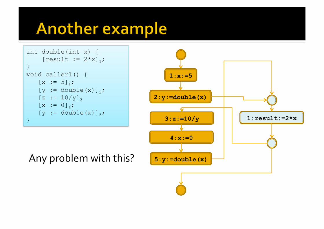
  Example:  Zero  analysis    Default:  MZ  (top)  for  all  arguments  and  results  ▪  Meaning:  The  method  can  receive  any  value  and  return  any  value  

  Benefit:    All  parameters  and  result  satisfy  this  assumption    Cost:  Too  conservative  wrt.  the  actual  input/output  ▪  Many  false  positives  

  divByX  analysis  int divByX(int x) { [result := 10/x]1; } void caller1() { [x := 5]1; [y := divByX(x)]2; }

pos   x   Result  

0   MZ   ⊥  

1   MZ   NZ  

  It  holds  σ(result)⊆MZ    Warning:  div  by  zero  at  #1  

  Caller1  Analysis  pos   x   y  

0   ⊥   ⊥  

1   NZ   ⊥  

2   NZ   MZ  

  It  holds  σ(x)⊆MZ  

  We  assume  x  must  be  MZ  and  result  is  MZ  

  Problem:  div  by  zero  is  not  possible!  

  divByX  analysis  int divByX(int x) { [result := 10/x]1; } void caller1() { [x := 5]1; [y := divByX(x)]2; }

pos   x   Result  

0   NZ   ⊥  

1   NZ   NZ  

  No  warning  s    It  holds  σ(result)⊆NZ  

  Caller1  analysis  pos   x   y  

0   ⊥   ⊥  

1   NZ   ⊥  

2   NZ   NZ  

  It  holds  σ(x)⊆NZ  

  We  assume  x  must  be  NZ  and  result  must  be  NZ  

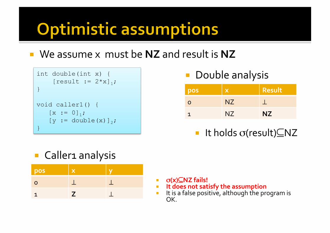
  Double  analysis  int double(int x) { [result := 2*x]1; } void caller1() { [x := 0]1; [y := double(x)]2; }

pos   x   Result  

0   NZ   ⊥  

1   NZ   NZ  

  It  holds  σ(result)⊆NZ  

  Caller1  analysis  pos   x   y  

0   ⊥   ⊥  

1   Z   ⊥  

2   Z   NZ  

  σ(x)⊆NZ  fails!    It  does  not  satisfy  the  assumption    It  is  a  false  positive,  although  the  program  is  

OK.  

  We  assume  x    must  be  NZ  and  result  is  NZ  

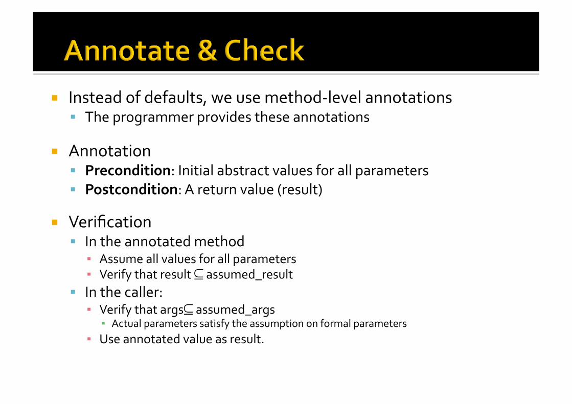
  Instead  of  defaults,  we  use  method-­‐level  annotations    The  programmer  provides  these  annotations  

  Annotation    Precondition:  Initial  abstract  values  for  all  parameters    Postcondition:  A  return  value  (result)  

  Verification    In  the  annotated  method  ▪  Assume  all  values  for  all  parameters  ▪  Verify  that  result  ⊆  assumed_result  

  In  the  caller:  ▪  Verify  that  args⊆  assumed_args  ▪  Actual  parameters  satisfy  the  assumption  on  formal  parameters  

▪  Use  annotated  value  as  result.  

  divByX  Analysis  @NZ int divByX(@NZ int x) { [result := 10/x]1; } void caller1() { [x := 5]1; [y := divByX(x)]2; }

pos   x   Result  

0   NZ   ⊥  

1   NZ   NZ  

  It  holds  σ(result)⊆NZ  

  Caller1  analysis  pos   x   y  

0   ⊥   ⊥  

1   NZ   ⊥  

2   NZ   NZ  

  It  verifies  that  σ(x)⊆NZ  

  double  analysis  @NZ int double(@NZ int x) { [result := 2*x]1; } void caller1() { [x := o]1; [y := double(x)]2; }

pos   x   Result  

0   NZ   ⊥  

1   NZ   NZ  

  It  holds  σ(result)⊆NZ  

  σ(x)⊆NZ  fails!    The  double  precondition  is  not  met    It  is  a  false  positive,  although  the  program  is  

OK  

  Caller1  analysis  pos   x   y  

0   ⊥   ⊥  

1   Z   ⊥  

2  

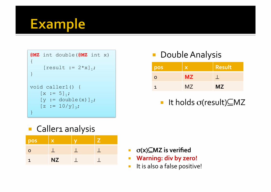
pos   x   y   Z  

0   ⊥   ⊥   ⊥  

1   NZ   ⊥   ⊥  

2   NZ   MZ   ⊥  

3   NZ   MZ   MZ  

  Double  Analysis  @MZ int double(@MZ int x) { [result := 2*x]1; } void caller1() { [x := 5]1; [y := double(x)]2; [z := 10/y]3; }

pos   x   Result  

0   MZ   ⊥  

1   MZ   MZ  

  It  holds  σ(result)⊆MZ  

  Caller1  analysis  

  σ(x)⊆MZ  is  verified    Warning:  div  by  zero!    It  is  also  a  false  positive!  

 We  have  to  distinguish  among  several  context  calls  

 Many  techniques  for  this:    Inlining/Cloning    Call  chains    Assume/  Guarantee   Method  Summaries  

  Idea:    Compute  a  unique  summary  for  each  method   Map  dataflow  input  information  to  dataflow  output  information  

  Context  sensitive    Given  different  input,  they  output  different  results    Instantiate  the  summary  on  each  method  invokation  

  Abstract  Summaries    Represent  symbollically  the  effect  of  the  function  over  the  elements  of  the  lattice  

pos   x   Y   Z  

0   ⊥   ⊥   ⊥  

1   NZ   ⊥   ⊥  

2   NZ   NZ   ⊥  

double:    case  x:NZresult:NZ  pos   x   Result  

0   NZ   ⊥  

1   NZ   NZ  

  Caller1  analysis  

int double(int x) { [result := 2*x]1; } void caller1() { [x := 5]1; [y := double(x)]2; [z := 10/y]3 [x := 0]4; [y := double(x)]5; }

4   Z   NZ   NZ  

5   Z   Z   MZ  

3   NZ   NZ   NZ  

double:    case  x:Zresult:Z  pos   x   Result  

0   Z   ⊥  

1   Z   Z  

• Case  x:NZ    result:  NZ  • Case  x:Z    result:  Z  

Verify:    case  x:NZresult:NZ  pos   x   Result  

0   NZ   ⊥  

1   NZ   NZ  

  Verify  for  caller  1      Case      x:NZ  Pos   x   y   Z  

1   NZ   ⊥   ⊥  

2   NZ   NZ   ⊥  

@Case(“x:NZ -> result:NZ”) @Case(“x:Z -> result:Z”) int double(int x) { [result := 2*x]1; } void caller1() { [x := 5]1; [y := double(x)]2; [z := 10/y]3 [x := 0]4; [y := double(x)]5; }

4   Z   NZ   NZ  

5   Z   Z   NZ  

verify:    case  x:Zresult:Z  pos   x   Result  

0   Z   ⊥  

1   Z   Z  

  Verify  for  caller  1    Case      x:Z  

pos   x   y   Z  

0   ⊥   ⊥   ⊥  

1   NZ   ⊥   ⊥  

2   NZ   NZ   ⊥  

double:  pos   x   Result  

0   A   ⊥  

1   A   A  

  Caller1  Analysis  

int double(int x) { [result := 2*x]1; } void caller1() { [x := 5]1; [y := double(x)]2; [z := 10/y]3 [x := 0]4; [y := double(x)]5; }

4   Z   NZ   NZ  

5   Z   Z   MZ  

3   NZ   NZ   NZ  

Summary:  Case  x:  A    result:  A  

A=NZ  

A=Z  

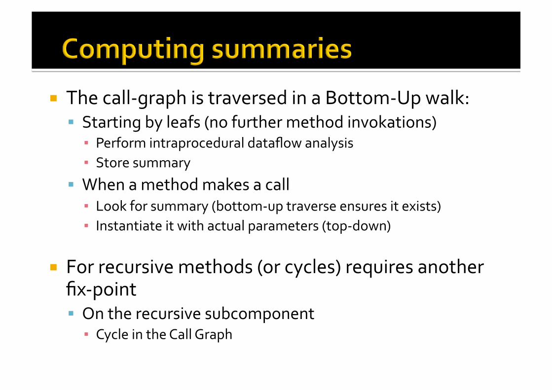
  The  call-­‐graph  is  traversed  in  a  Bottom-­‐Up  walk:    Starting  by  leafs  (no  further  method  invokations)  ▪  Perform  intraprocedural  dataflow  analysis  ▪  Store  summary  

  When  a  method  makes  a  call  ▪  Look  for  summary  (bottom-­‐up  traverse  ensures  it  exists)  ▪  Instantiate  it  with  actual  parameters  (top-­‐down)  

  For  recursive  methods  (or  cycles)  requires  another  fix-­‐point    On  the  recursive  subcomponent  ▪  Cycle  in  the  Call  Graph  

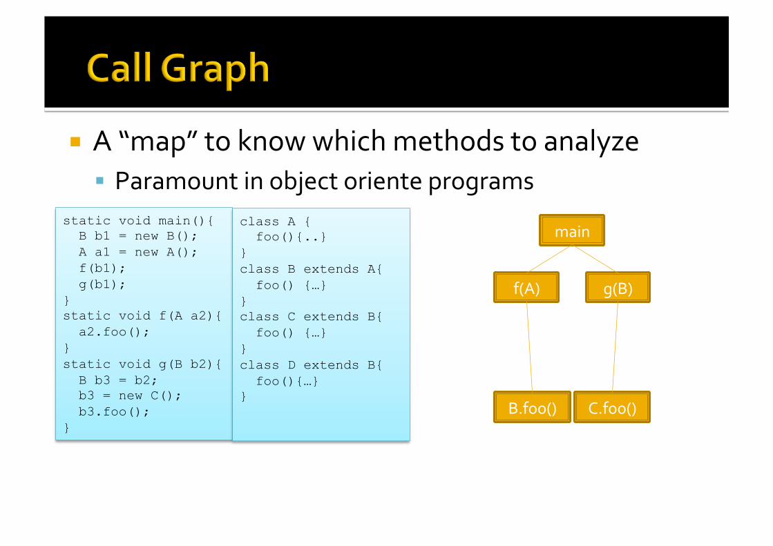
  A  “map”  to  know  which  methods  to  analyze    Paramount  in  object  oriente  programs  

static void main(){ B b1 = new B(); A a1 = new A(); f(b1); g(b1); } static void f(A a2){ a2.foo(); } static void g(B b2){ B b3 = b2; b3 = new C(); b3.foo(); }

class A { foo(){..} } class B extends A{ foo() {…} } class C extends B{ foo() {…} } class D extends B{ foo(){…} }

main  

f(A)   g(B)  

B.foo()   C.foo()  

  A  “map”  to  know  which  methods  to  analyze    Paramount  in  object  oriente  programs  

static void main(){ B b1 = new B(); A a1 = new A(); f(b1); g(b1); } static void f(A a2){ a2.foo(); } static void g(B b2){ B b3 = b2; b3 = new C(); b3.foo(); }

class A { foo(){..} } class B extends A{ foo() {…} } class C extends B{ foo() {…} } class D extends B{ foo(){…} }

main  

f(A)   g(B)  

B.foo()   C.foo()   D.foo()  A.foo()  

Computed  using  Class  Hierarchy  Analysis  (CHA)  

  A  “map”  to  know  which  methods  to  analyze    Paramount  in  object  oriente  programs  

static void main(){ B b1 = new B(); A a1 = new A(); f(b1); g(b1); } static void f(A a2){ a2.foo(); } static void g(B b2){ B b3 = b2; b3 = new C(); b3.foo(); }

class A { foo(){..} } class B extends A{ foo() {…} } class C extends B{ foo() {…} } class D extends B{ foo(){…} }

main  

f(A)   g(B)  

B.foo()   C.foo()  A.foo()  

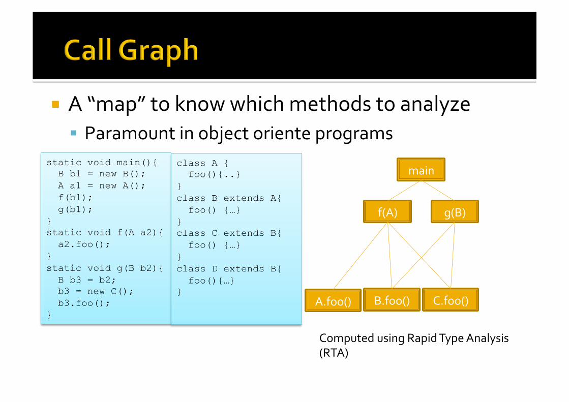
Computed  using  Rapid  Type  Analysis  (RTA)  

  A  “map”  to  know  which  methods  to  analyze    Paramount  in  object  oriente  programs  

static void main(){ B b1 = new B(); A a1 = new A(); f(b1); g(b1); } static void f(A a2){ a2.foo(); } static void g(B b2){ B b3 = b2; b3 = new C(); b3.foo(); }

class A { foo(){..} } class B extends A{ foo() {…} } class C extends B{ foo() {…} } class D extends B{ foo(){…} }

main  

f(A)   g(B)  

B.foo()   C.foo()  A.foo()  

Computed  using  XTA  

  Assumptions    Simple  &  efficient    Imprecise  (too  general)  

  Annotations    Requires  effort    More  precise  than  assumptions    More  efficient  than  

interprocedural  analysis    A  whole-­‐program  analysis  is  

not  required!  

  CFG  Interprocedural    Easy  to  implement    Imprecise    Can  be  too  expensive     As  precise  as  simple  

  Summaries    Very  precise    Vert  expensive  if  no  abstraction  

is  done    They  require  whole-­‐program  

analysis  

  Compilers:  Principles,  Tecniques  &Tools  2nd  Edition:  Aho,  Lam,  Sethi,  Ullman  

  Principles  of  Program  Analysis  .  Flemming  Nielson,  Hanne  Riis  Nielson,  Chris  Hankin.  

  Modern  compiler  implementation  in  Java.  Andrew  Appel.  2nd  Edition.