Embed Size (px)
Citation preview
Interprocedural Analysis
CS252r Spring 2011
© 2010 Stephen Chong, Harvard University
Procedures
•So far looked at intraprocedural analysis: analyzing a single procedure
•Interprocedural analysis uses calling relationships among procedures
•Enables more precise analysis information
2
© 2010 Stephen Chong, Harvard University
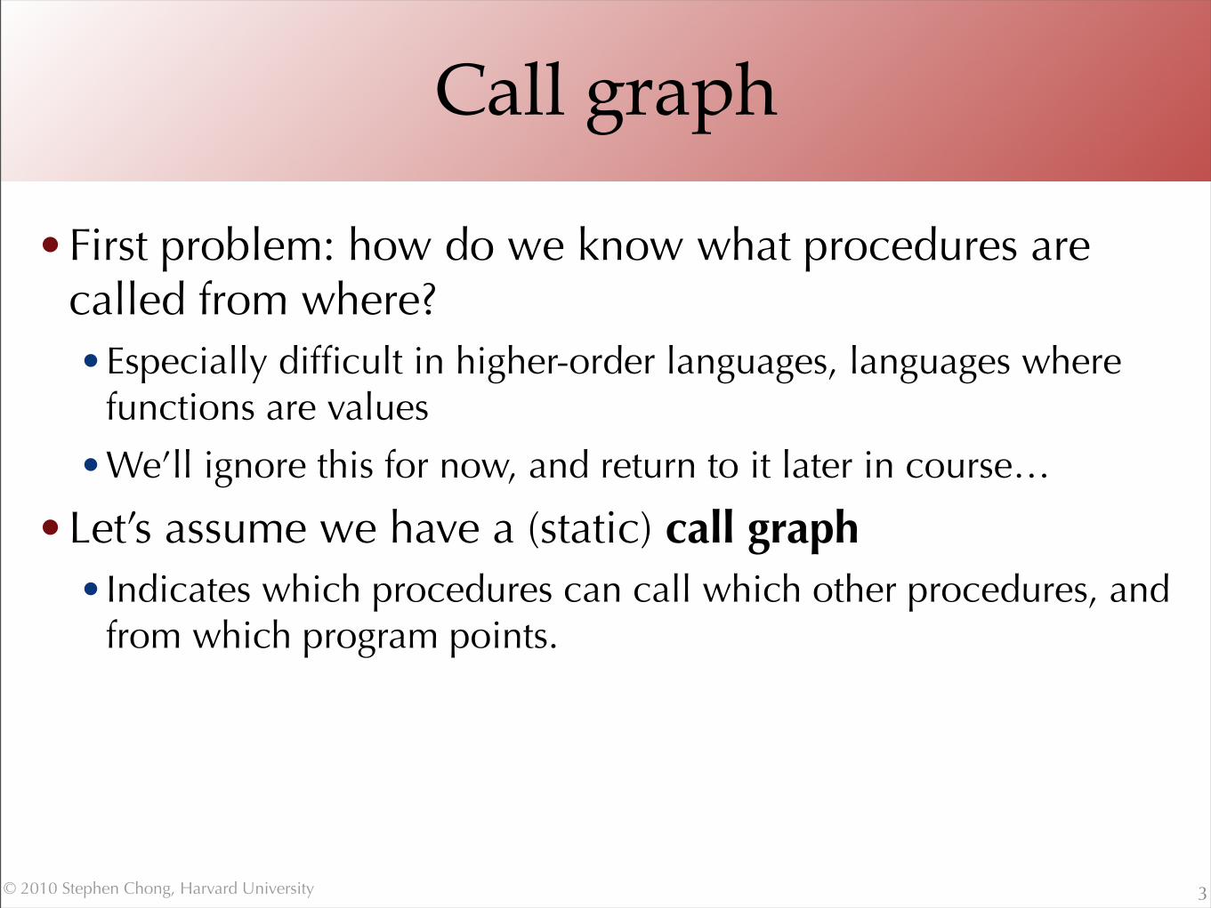
Call graph
•First problem: how do we know what procedures are called from where? •Especially difficult in higher-order languages, languages where
functions are values
•We’ll ignore this for now, and return to it later in course…
•Let’s assume we have a (static) call graph•Indicates which procedures can call which other procedures, and
from which program points.
3

© 2010 Stephen Chong, Harvard University
Call graph example
4
f() { 1: g(); 2: g(); 3: h();}
g() { 4: h();}
h() { 5: f(); 6: i();}
i() { … }
12
3 5
6
4
f
gh
i
© 2010 Stephen Chong, Harvard University
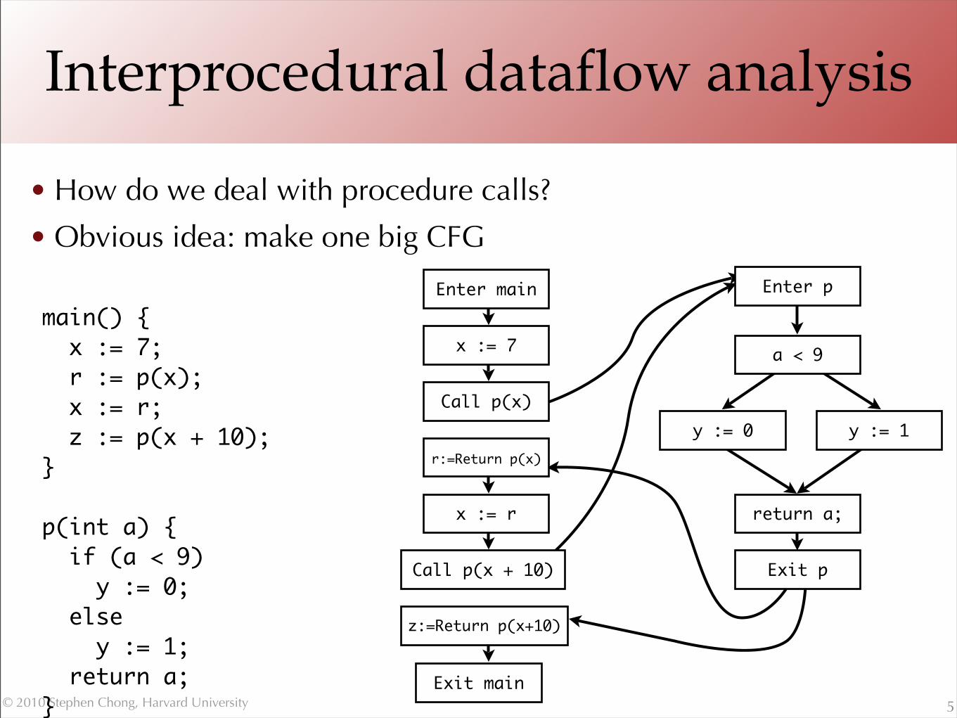
Interprocedural dataflow analysis
• How do we deal with procedure calls?
• Obvious idea: make one big CFG
5
main() { x := 7; r := p(x); x := r; z := p(x + 10);}
p(int a) { if (a < 9) y := 0; else y := 1; return a;}
Exit main
Enter main
x := 7
Call p(x)
r:=Return p(x)
x := r
Call p(x + 10)
z:=Return p(x+10)
Enter p
a < 9
y := 0 y := 1
Exit p
return a;
© 2010 Stephen Chong, Harvard University
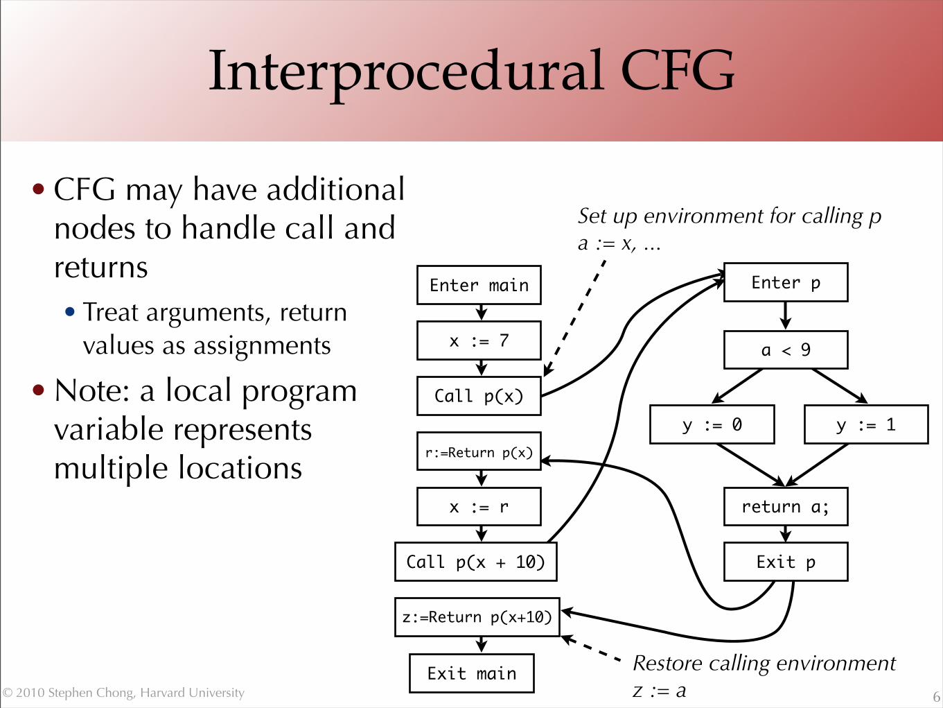
Interprocedural CFG
• CFG may have additional nodes to handle call and returns• Treat arguments, return
values as assignments
• Note: a local program variable represents multiple locations
6
Set up environment for calling pa := x, ...
Restore calling environment z := a
Exit main
Enter main
x := 7
Call p(x)
r:=Return p(x)
x := r
Call p(x + 10)
z:=Return p(x+10)
Enter p
a < 9
y := 0 y := 1
Exit p
return a;
© 2010 Stephen Chong, Harvard University
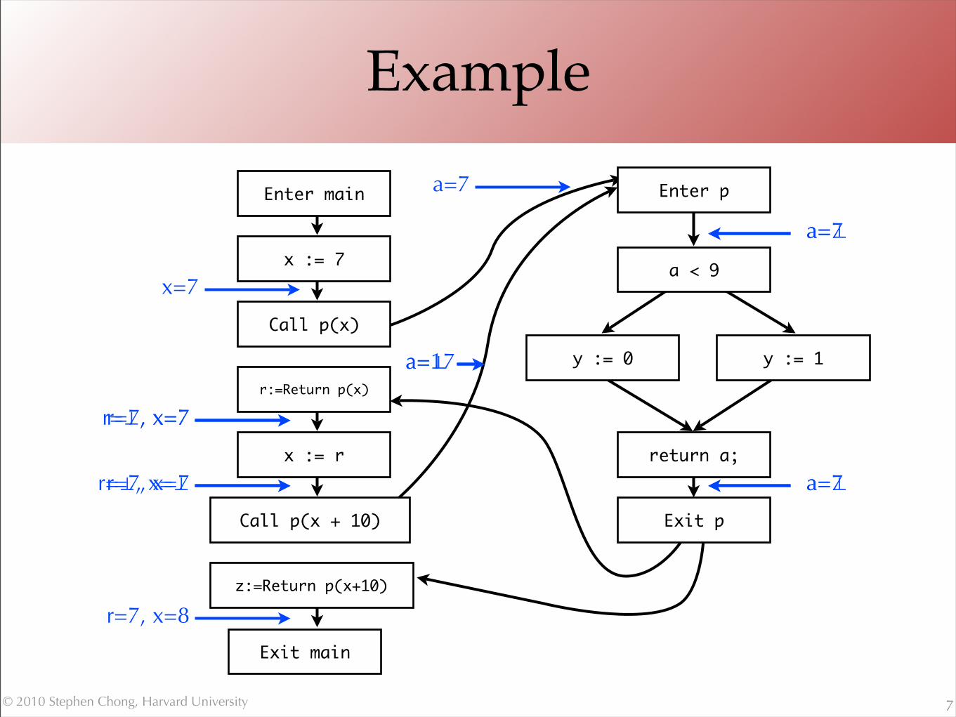
Example
7
Exit main
Enter main
x := 7
Call p(x)
r:=Return p(x)
x := r
Call p(x + 10)
z:=Return p(x+10)
Enter p
a < 9
y := 0 y := 1
Exit p
return a;
x=7
a=7
a=7
a=7
r=7, x=7
r=7, x=7
a=17
a=⊥
a=⊥
r=7, x=8
r=⊥, x=7
r=⊥, x=⊥
a=⊥
© 2010 Stephen Chong, Harvard University
Invalid paths
•Problem: dataflow facts from one call site “tainting” results at other call site•p analyzed with merge of dataflow facts from all call
sites
•How to address?
8
© 2010 Stephen Chong, Harvard University
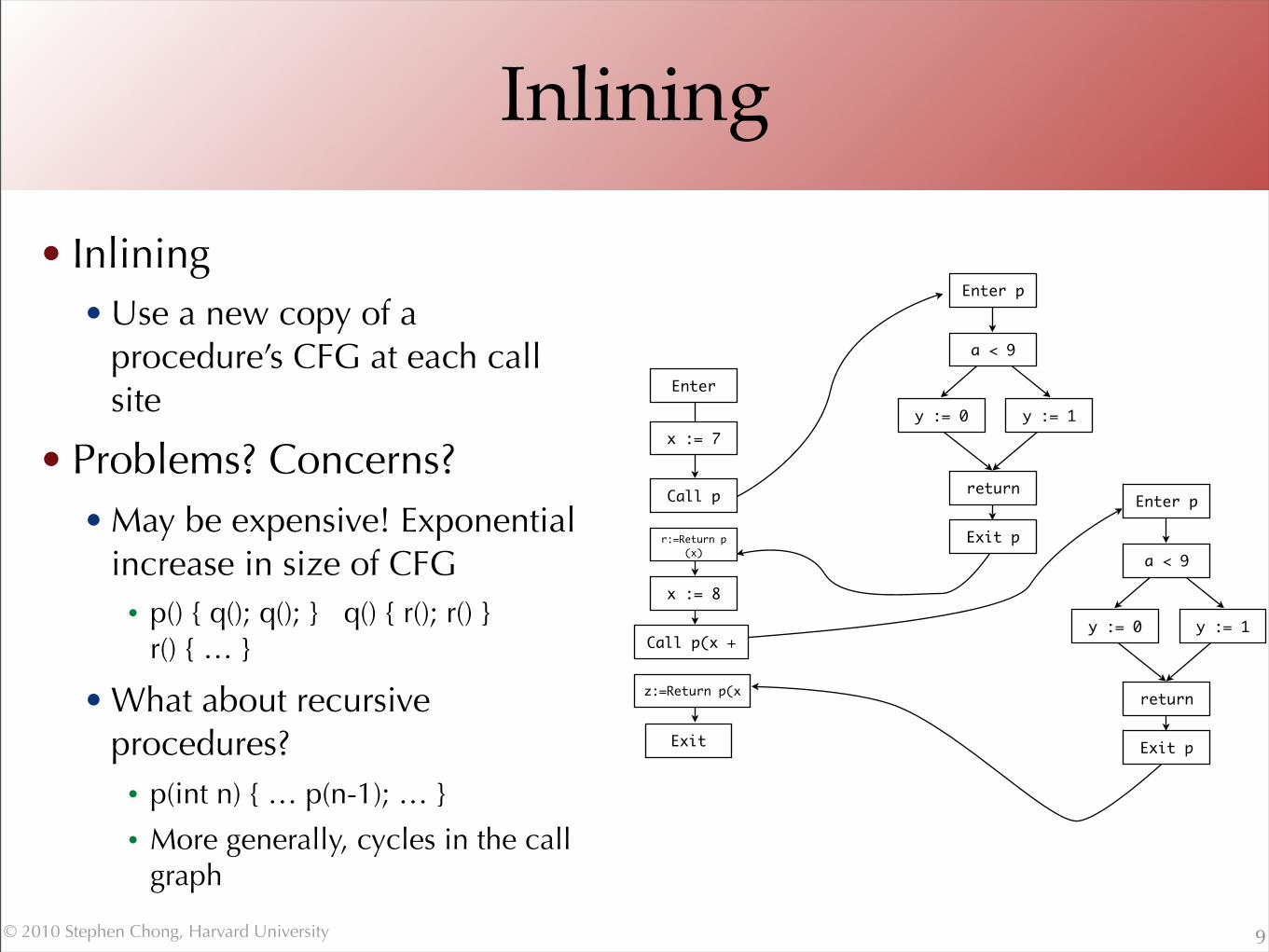
Inlining
• Inlining• Use a new copy of a
procedure’s CFG at each call site
• Problems? Concerns?• May be expensive! Exponential
increase in size of CFG• p() { q(); q(); } q() { r(); r() }
r() { … }
• What about recursive procedures?• p(int n) { … p(n-1); … }
• More generally, cycles in the call graph
9
Exit
Enter
x := 7
Call p
r:=Return p(x)
x := 8
Call p(x +
z:=Return p(x
Enter p
a < 9
y := 0 y := 1
Exit p
return Enter p
a < 9
y := 0 y := 1
Exit p
return
© 2010 Stephen Chong, Harvard University
Context sensitivity
•Solution: make a finite number of copies•Use context information to determine when to
share a copy•Results in a context-sensitive analysis
•Choice of what to use for context will produce different tradeoffs between precision and scalability
•Common choice: approximation of call stack
10
© 2010 Stephen Chong, Harvard University
Context sensitivity example
11
main() { 1: p(); 2: p();}
p() { 3: q();} q() { …}
Exit p
Enter p
3: Call q()
3: Return q()
Context: 1
Exit q
Enter q
...
Context: 3
Exit main
Enter main
1: Call p()
1: Return p()
2: Call p()
2: Return p()
Context: -
Exit p
Enter p
3: Call q()
3: Return q()
Context: 2
© 2010 Stephen Chong, Harvard University
Context sensitivity example
12
main() { 1: p(); 2: p();}
p() { 3: q();} q() { …}
Exit p
Enter p
3: Call q()
3: Return q()
Context: 1::-
Exit q
Enter q
...
Context: 3::1
Exit main
Enter main
1: Call p()
1: Return p()
2: Call p()
2: Return p()
Context: -
Exit p
Enter p
3: Call q()
3: Return q()
Context: 2::-
Exit q
Enter q
...
Context: 3::2

© 2010 Stephen Chong, Harvard University
Fibonacci: context insensitive
13
main() { 1: fib(7);}
fib(int n) { if n <= 1 x := 0 else 2: y := fib(n-1); 3: z := fib(n-2); x:= y+z; return x;}
Exit
Enter
2
Exit
Enter
1: call
1: return
© 2010 Stephen Chong, Harvard University
Fibonacci: context sensitive, stack depth 1
14
main() { 1: fib(7);}
fib(int n) { if n <= 1 x := 0 else 2: y := fib(n-1); 3: z := fib(n-2); x:= y+z; return x;}
Exit
Enter
1: call
1: return
Context: -
Exit
Enter
Context: 1
2
Exit
Enter
Context: 2
2
Exit
Enter
Context: 3
2

© 2010 Stephen Chong, Harvard University
Fibonacci: context sensitive, stack depth 2
15
main() { 1: fib(7);}
fib(int n) { if n <= 1 x := 0 else 2: y := fib(n-1); 3: z := fib(n-2); x:= y+z; return x;}
Exit
Enter
1: call
1: return
Context: -
Context: 1::-
Exit
Enter2
Context: 2::1
Exit
Enter2
Context: 3::1
Exit
Enter2
Context: 2::2
Exit
Enter2
Context: 3::2
Exit
Enter2
Context: 2::3
Exit
Enter2
Context: 3::3
Exit
Enter2
© 2010 Stephen Chong, Harvard University
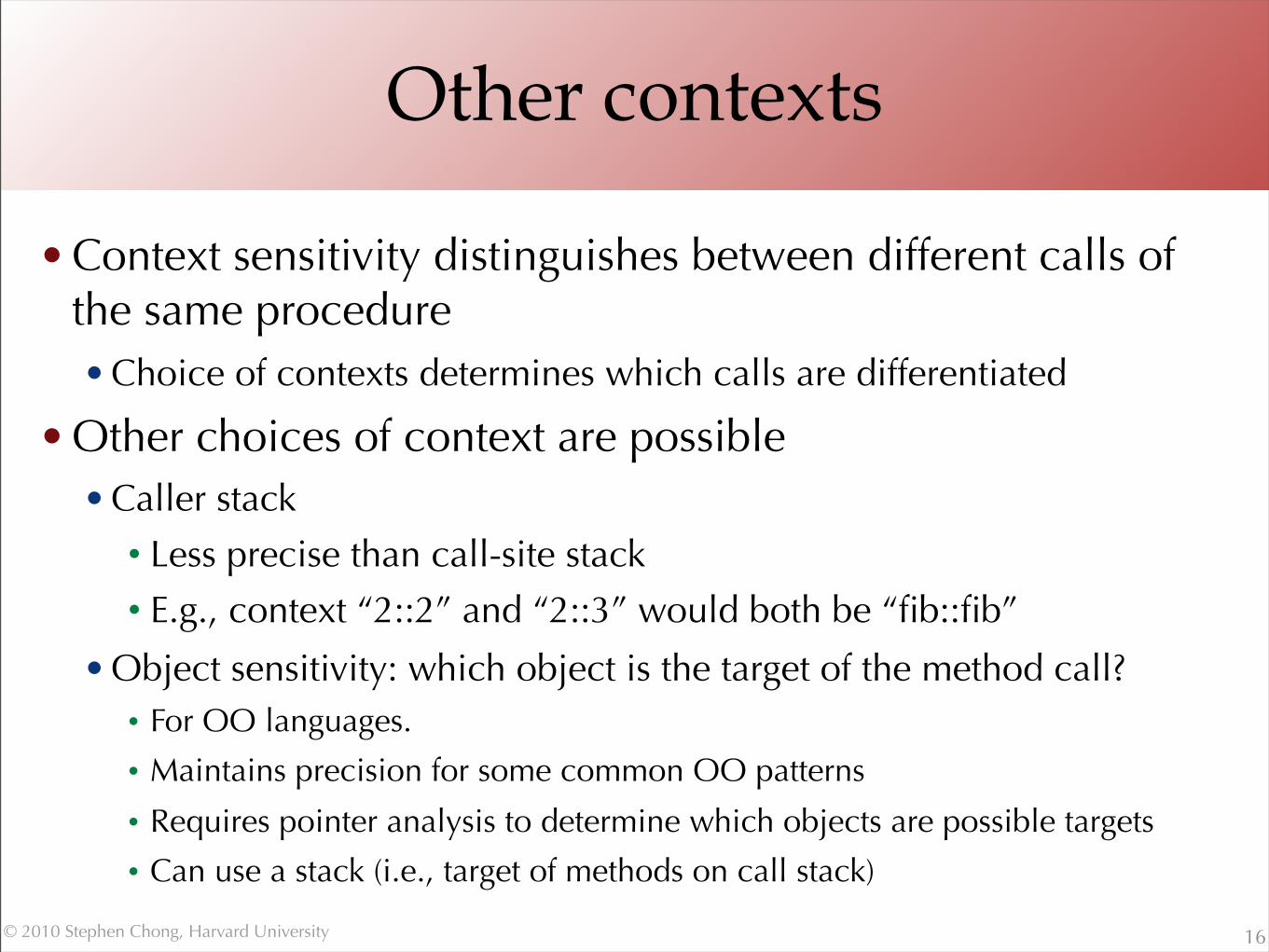
Other contexts
• Context sensitivity distinguishes between different calls of the same procedure• Choice of contexts determines which calls are differentiated
• Other choices of context are possible• Caller stack
• Less precise than call-site stack
• E.g., context “2::2” and “2::3” would both be “fib::fib”
• Object sensitivity: which object is the target of the method call?• For OO languages.
• Maintains precision for some common OO patterns
• Requires pointer analysis to determine which objects are possible targets
• Can use a stack (i.e., target of methods on call stack)
16
© 2010 Stephen Chong, Harvard University
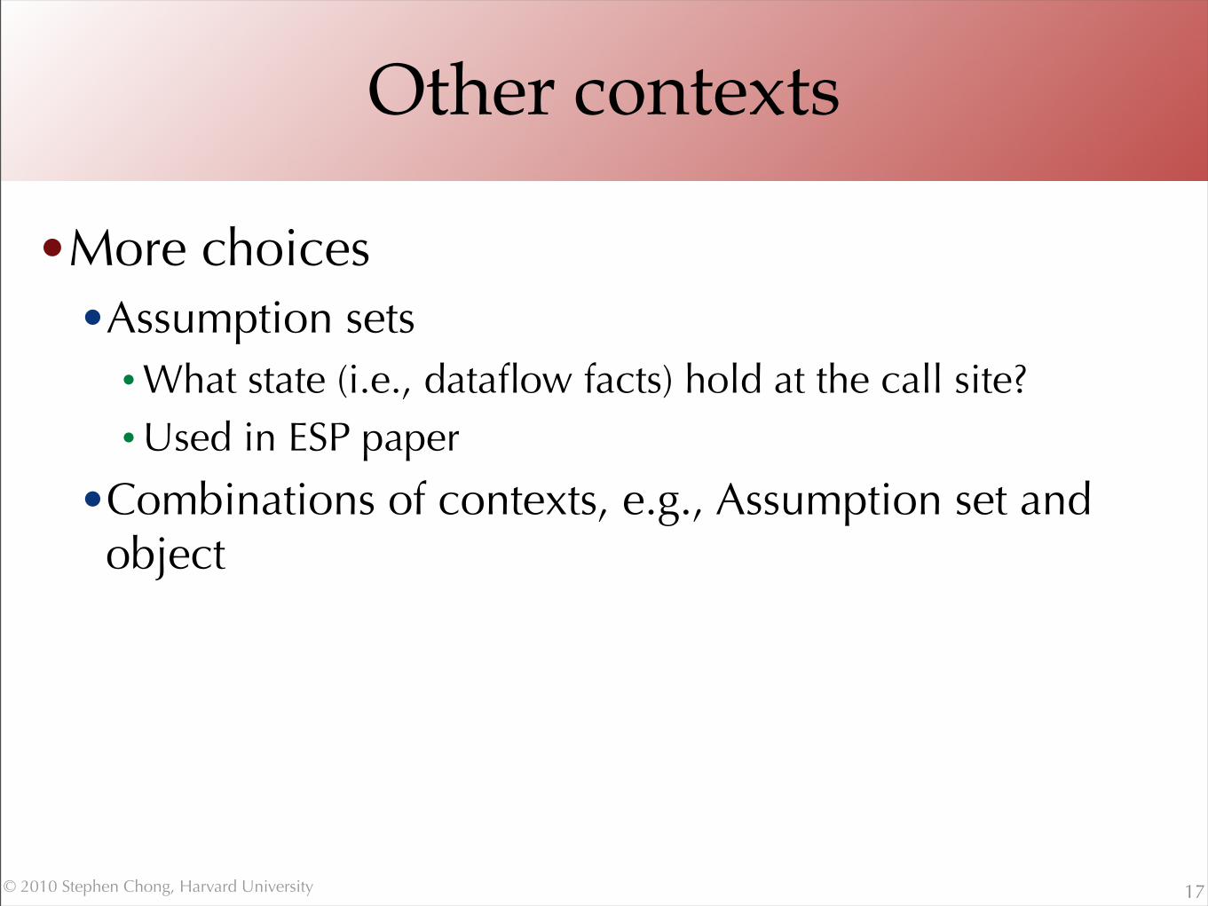
Other contexts
•More choices•Assumption sets•What state (i.e., dataflow facts) hold at the call site?•Used in ESP paper
•Combinations of contexts, e.g., Assumption set and object
17
© 2010 Stephen Chong, Harvard University
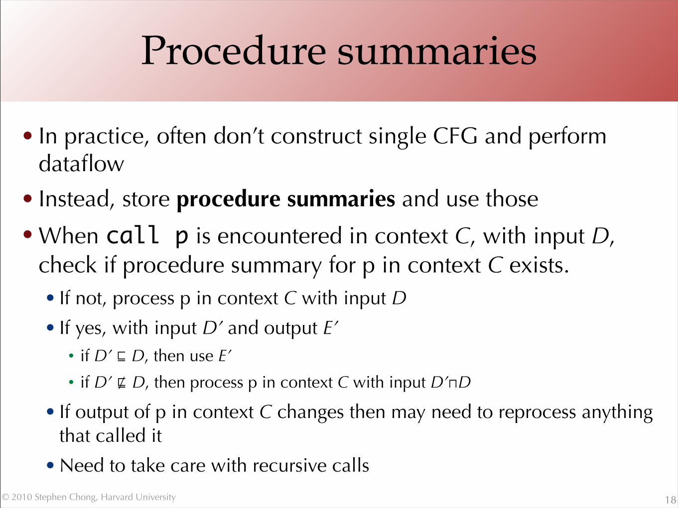
Procedure summaries
• In practice, often don’t construct single CFG and perform dataflow
• Instead, store procedure summaries and use those
• When call p is encountered in context C, with input D, check if procedure summary for p in context C exists.• If not, process p in context C with input D
• If yes, with input D’ and output E’• if D’ ⊑ D, then use E’
• if D’ ⋢ D, then process p in context C with input D’⊓D
• If output of p in context C changes then may need to reprocess anything that called it
• Need to take care with recursive calls
18
© 2010 Stephen Chong, Harvard University
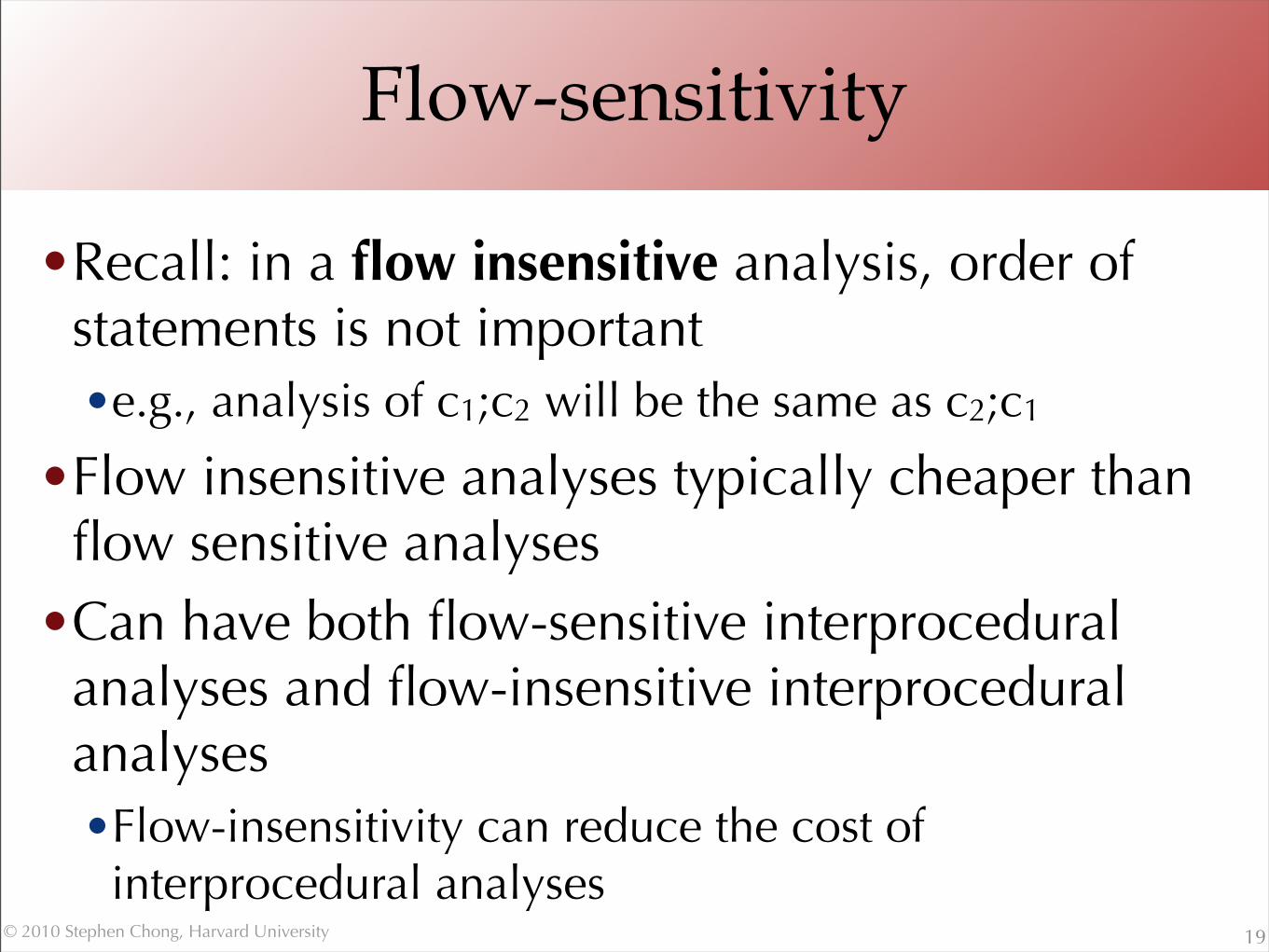
Flow-sensitivity
•Recall: in a flow insensitive analysis, order of statements is not important•e.g., analysis of c1;c2 will be the same as c2;c1
•Flow insensitive analyses typically cheaper than flow sensitive analyses
•Can have both flow-sensitive interprocedural analyses and flow-insensitive interprocedural analyses•Flow-insensitivity can reduce the cost of
interprocedural analyses19
© 2010 Stephen Chong, Harvard University
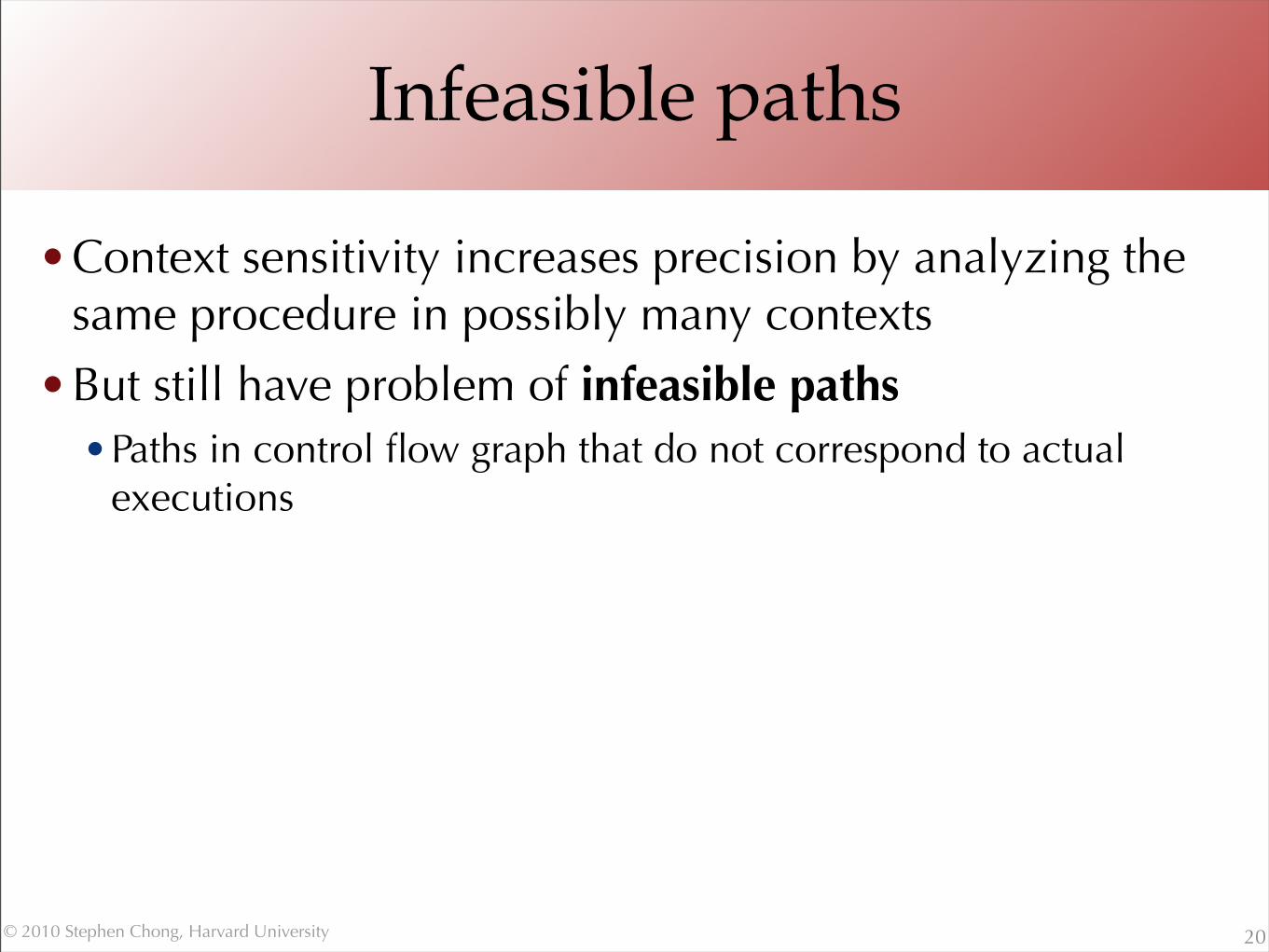
Infeasible paths
•Context sensitivity increases precision by analyzing the same procedure in possibly many contexts
•But still have problem of infeasible paths•Paths in control flow graph that do not correspond to actual
executions
20
© 2010 Stephen Chong, Harvard University
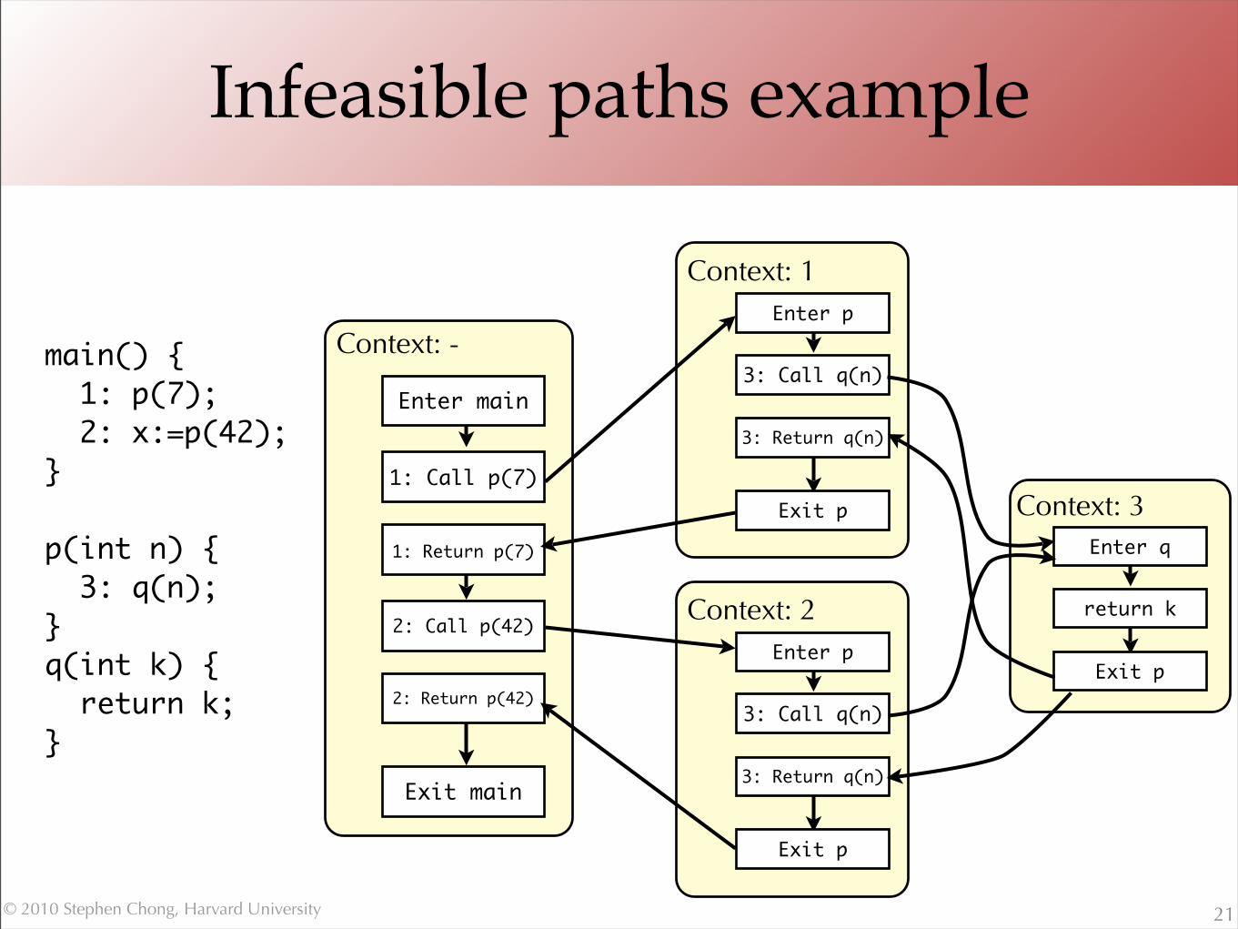
Infeasible paths example
21
main() { 1: p(7); 2: x:=p(42);}
p(int n) { 3: q(n);} q(int k) { return k;}
Exit p
Enter p
3: Call q(n)
3: Return q(n)
Context: 1
Exit p
Enter q
return k
Context: 3
Exit main
Enter main
1: Call p(7)
1: Return p(7)
2: Call p(42)
2: Return p(42)
Context: -
Exit p
Enter p
3: Call q(n)
3: Return q(n)
Context: 2
© 2010 Stephen Chong, Harvard University
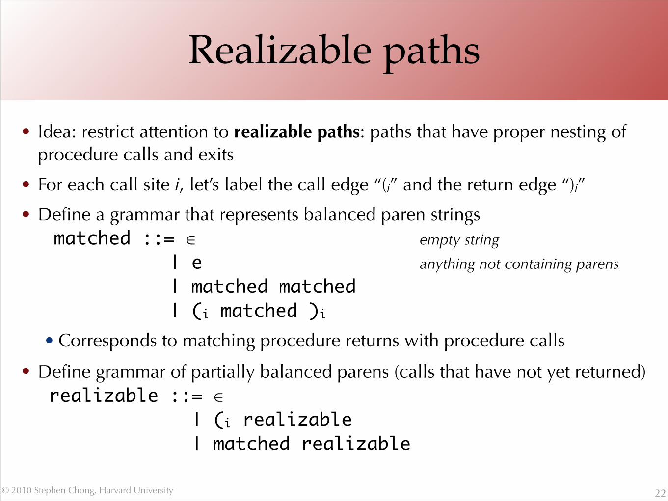
Realizable paths
• Idea: restrict attention to realizable paths: paths that have proper nesting of procedure calls and exits
• For each call site i, let’s label the call edge “(i” and the return edge “)i”
• Define a grammar that represents balanced paren strings matched ::= ∈ empty string
| e anything not containing parens
| matched matched | (i matched )i• Corresponds to matching procedure returns with procedure calls
• Define grammar of partially balanced parens (calls that have not yet returned) realizable ::= ∈ | (i realizable | matched realizable
22

© 2010 Stephen Chong, Harvard University
Example
23
main() { 1: p(7); 2: x:=p(42);}
p(int n) { 3: q(n);} q(int k) { return k;}
Exit p
Enter p
3: Call q(n)
3: Return q(n)
Exit p
Enter q
return k
Exit main
Enter main
1: Call p(7)
1: Return p(7)
2: Call p(42)
2: Return p(42)
(1(3
(2
)1
)2
)3
© 2010 Stephen Chong, Harvard University
Meet over Realizable Paths
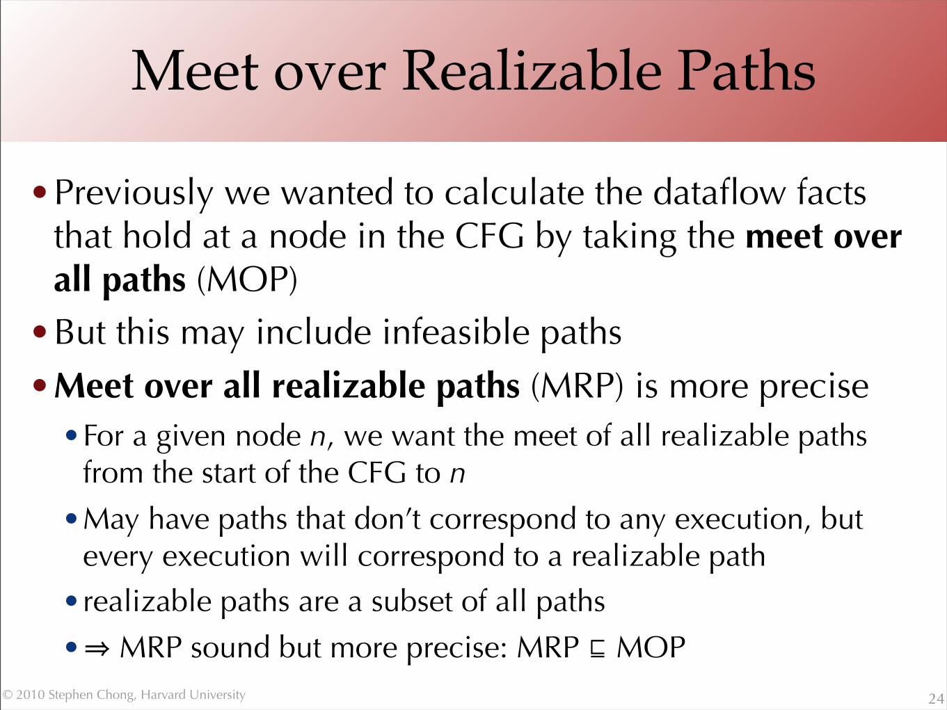
•Previously we wanted to calculate the dataflow facts that hold at a node in the CFG by taking the meet over all paths (MOP)
•But this may include infeasible paths
•Meet over all realizable paths (MRP) is more precise•For a given node n, we want the meet of all realizable paths
from the start of the CFG to n
•May have paths that don’t correspond to any execution, but every execution will correspond to a realizable path
•realizable paths are a subset of all paths
•⇒ MRP sound but more precise: MRP ⊑ MOP
24
© 2010 Stephen Chong, Harvard University
Program analysis as CFL reachability
•Can phrase many program analyses as context-free language reachability problems in directed graphs•“Program Analysis via Graph Reachability” by Thomas
Reps, 1998• Summarizes a sequence of papers developing this idea
25
© 2010 Stephen Chong, Harvard University
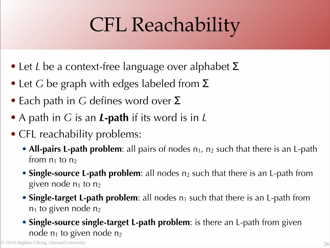
CFL Reachability
• Let L be a context-free language over alphabet Σ• Let G be graph with edges labeled from Σ• Each path in G defines word over Σ• A path in G is an L-path if its word is in L
• CFL reachability problems:• All-pairs L-path problem: all pairs of nodes n1, n2 such that there is an L-path
from n1 to n2
• Single-source L-path problem: all nodes n2 such that there is an L-path from given node n1 to n2
• Single-target L-path problem: all nodes n1 such that there is an L-path from n1 to given node n2
• Single-source single-target L-path problem: is there an L-path from given node n1 to given node n2
26
© 2010 Stephen Chong, Harvard University
Why bother?
•All CFL-reachability problems can be solved in time cubic in nodes of the graph
•Automatically get a faster, approximate solution: graph reachability
•On demand analysis algorithm for free•Gives insight into program analysis complexity
issues
27
© 2010 Stephen Chong, Harvard University
Encoding 1: IFDS problems
•Interprocedural finite distributive subset problems (IFDS problems)•Interprocedural dataflow analysis with• Finite set of data flow facts•Distributive dataflow functions ( f(a⊓b) = f(a) ⊓ f(b) )
•Can convert any IFDS problem as a CFL-graph reachability problem, and find the MRP solution with no loss of precision•May be some loss of precision phrasing problem as
IFDS28
© 2010 Stephen Chong, Harvard University
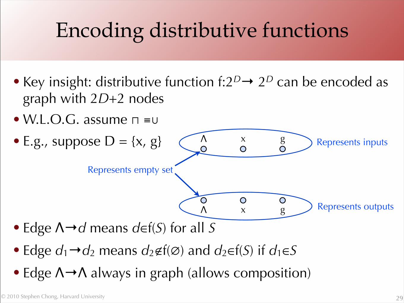
Encoding distributive functions
• Key insight: distributive function f:2D→ 2D can be encoded as graph with 2D+2 nodes
• W.L.O.G. assume ⊓ ≡∪
• E.g., suppose D = {x, g}
• Edge Λ→d means d∈f(S) for all S
• Edge d1→d2 means d2∉f(∅) and d2∈f(S) if d1∈S
• Edge Λ→Λ always in graph (allows composition)
29
Λ x g
Λ x g
Represents inputs
Represents outputs
Represents empty set
© 2010 Stephen Chong, Harvard University
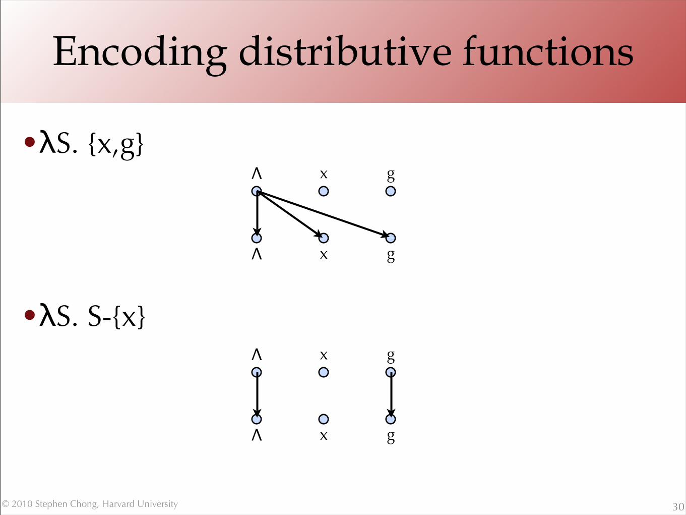
Encoding distributive functions
•λS. {x,g}
•λS. S-{x}
30
Λ x g
Λ x g
Λ x g
Λ x g
© 2010 Stephen Chong, Harvard University
Encoding distributive functions
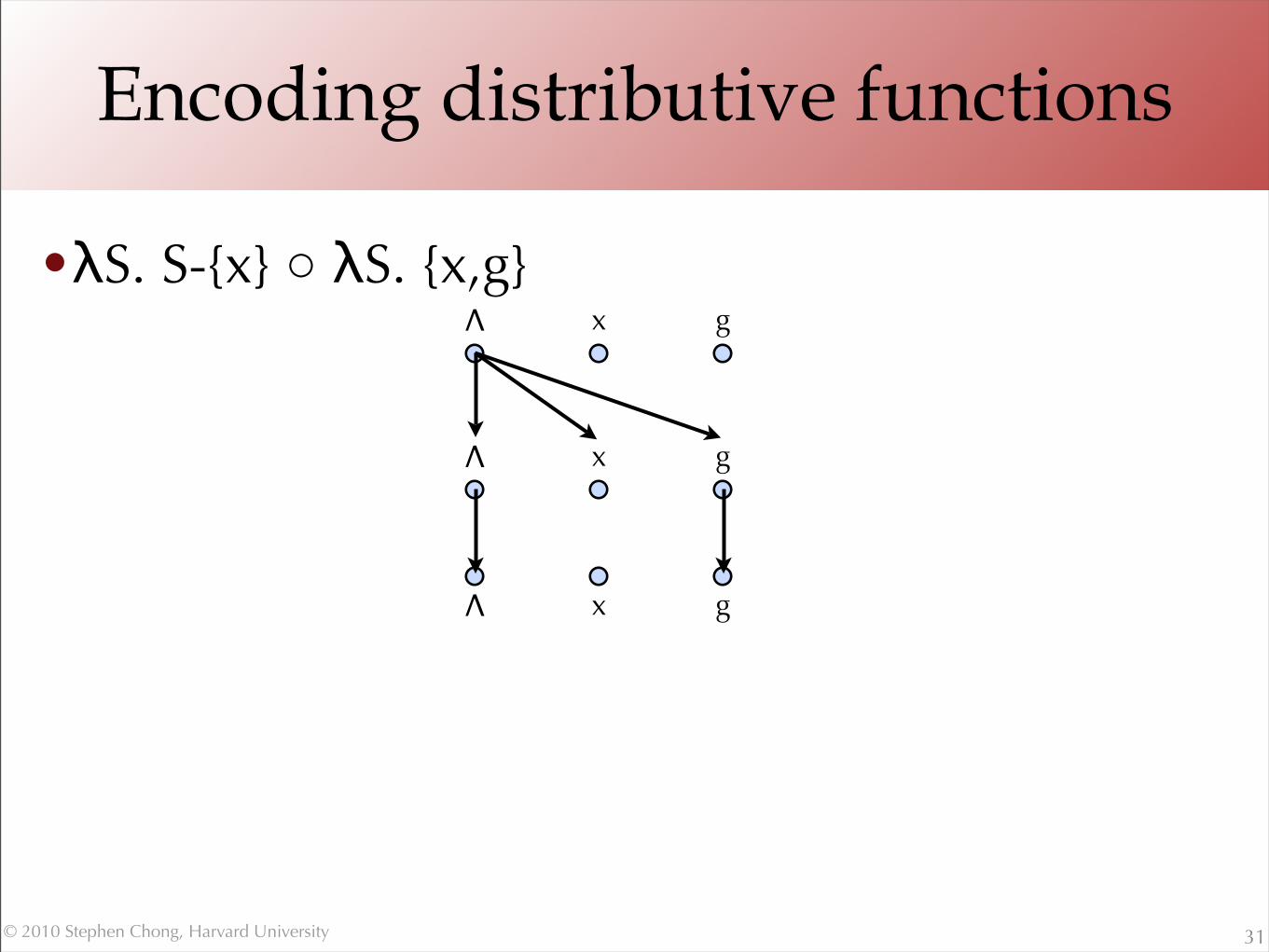
•λS. S-{x} ○ λS. {x,g}
31
Λ x g
Λ x g
Λ x g
© 2010 Stephen Chong, Harvard University
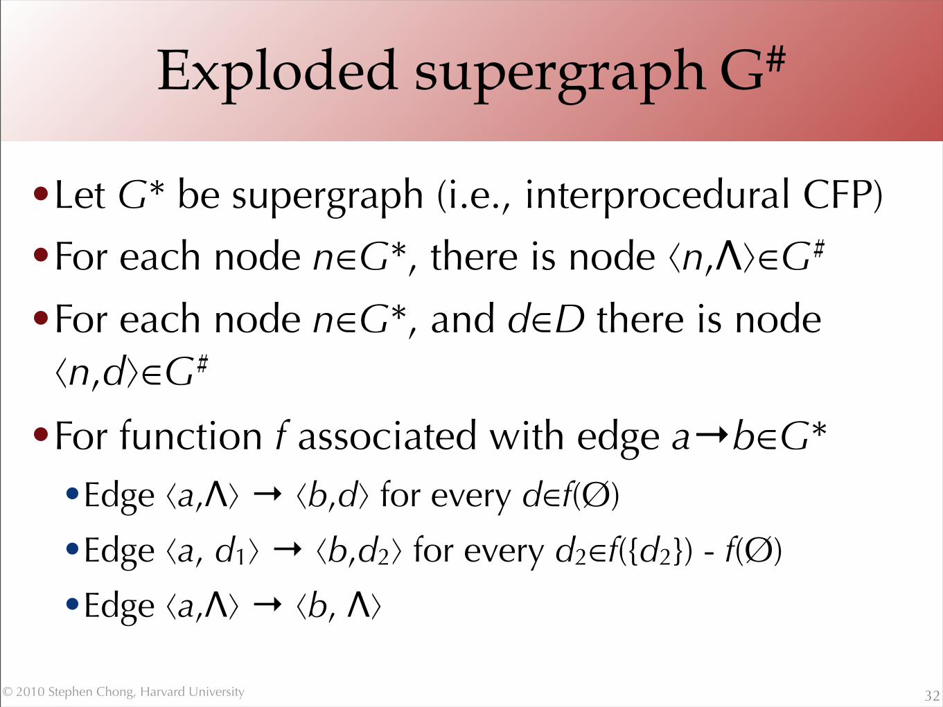
Exploded supergraph G#
•Let G* be supergraph (i.e., interprocedural CFP)
•For each node n∈G*, there is node ⟨n,Λ⟩∈G#
•For each node n∈G*, and d∈D there is node ⟨n,d⟩∈G#
•For function f associated with edge a→b∈G*•Edge ⟨a,Λ⟩ → ⟨b,d⟩ for every d∈f(Ø)
•Edge ⟨a, d1⟩ → ⟨b,d2⟩ for every d2∈f({d2}) - f(Ø)
•Edge ⟨a,Λ⟩ → ⟨b, Λ⟩
32
© 2010 Stephen Chong, Harvard University
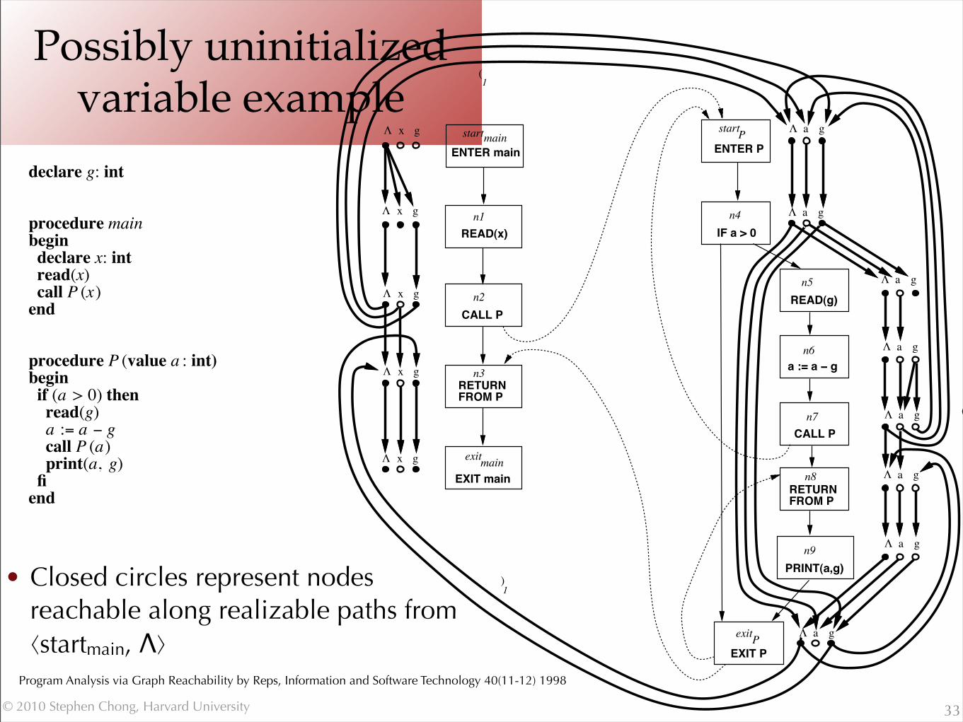
Possibly uninitialized variable example
33
! 5 !
declare g: int
procedure mainbegindeclare x: intread(x)call P (x)end
procedure P (value a : int)beginif (a > 0) thenread(g)a := a ! gcall P (a)print(a, g)fiend
"
"
"
"
"
"
"
"
"
"
"
"
"
"
"
"
S.S!{x}
S.S!{g}
S.S
S.S
S.S
S.S
S.S!{g}
S.S
S.S!{g}
S.S
ENTER PP
IF a > 0n4
ENTER mainmain
READ(x)n1
CALL Pn2
RETURNFROM P
n3
EXIT mainmain
RETURNFROM P
n8
EXIT P
CALL Pn7
n6a := a − g
n5READ(g)
PRINT(a,g)n9
S.{x,g}
S.if (a S) or (g S) then S {a} else S!{a}
U##
S.S<x/a>
S.S!{a}
S.S!{a}
S.S
start
exit
Pexit
start
(
)
(
)
1
1
2
2
(a) Example program (b) Supergraph G*
Fig. 1. An example program and its supergraph G* . The supergraph is annotated with the dataflow functions for the“possibly-uninitialized variables” problem. The notation S<x/a> denotes the set S with x renamed to a.
balanced by a preceding left parenthesis “(i”, but the converse need not hold.To understand these concepts, it helps to examine a few of the paths that occur in Fig. 1.The path “startmain $ n1$ n2$ startP $ n4$ exitP $ n3”, which has word “ee(1ee)1”, is a matchedpath (and hence a realizable path, as well). In general, a matched path from m to n, where m and n are inthe same procedure, represents a sequence of execution steps during which the call stack may tem-porarily grow deeper—because of calls—but never shallower than its original depth, before eventuallyreturning to its original depth.The path “startmain $ n1$ n2$ startP $ n4”, which has word “ee(1e”, is a realizable path but not amatched path: The call-to-start edge n2$ startP has no matching exit-to-return-site edge. A realizablepath from the program’s start node smain to a node n represents a sequence of execution steps that ends,in general, with some number of activation records on the call stack. The pending activation recordscorrespond to the unmatched (i’s in the path’s word.The path “startmain $ n1$ n2$ startP $ n4$ exitP $ n8”, which has word “ee(1ee)2”, is neither amatched path nor a realizable path: The exit-to-return-site edge exitP $ n8 does not correspond to thepreceding call-to-start edge n2$ startP. This path represents an infeasible execution path.
! 10 !
a g
ENTER PP
IF a > 0n4
ENTER mainmain
READ(x)n1
CALL Pn2
RETURNFROM P
n3
EXIT mainmain
RETURNFROM P
n8
EXIT PP
CALL Pn7
n6a := a − g
n5READ(g)
PRINT(a,g)n9
x g
x g
x g
x g
x g
a g
a g
a g
a g
a g
a g
a g
start
exit
exit
start"
"
"
"
"
"
"
"
"
"
"
"
"
(
)
(1
)1
2
2
Fig. 4. The exploded supergraph that corresponds to the instance of the possibly-uninitialized variables problem shownin Fig. 1. Closed circles represent nodes of G# that are reachable along realizable paths from #startmain ,"$. Open cir-cles represent nodes not reachable along such paths.
nodes #n8,g$ and #n9,g$ are reachable only along non-realizable paths from #startmain,"$.) This informa-tion indicates the nodes’ values in the meet-over-all-realizable-paths solution to the dataflow-analysis prob-lem. For instance, the meet-over-all-realizable-paths solution at node exitP is the set {g}. (That is, variableg is the only possibly-uninitialized variable just before execution reaches the exit node of procedure P.) InFig. 4, this information can be obtained by determining that there is a realizable path from #startmain,"$ to#exitP,g$, but not from #startmain ,"$ to #exitP,a$.
4.2. Interprocedural Program SlicingSlicing is an operation that identifies semantically meaningful decompositions of programs, where thedecompositions consist of elements that are not necessarily textually contiguous [98,72,32,46,77,92,19].Slicing, and subsequent manipulation of slices, has applications in many software-engineering tools,
Program Analysis via Graph Reachability by Reps, Information and Software Technology 40(11-12) 1998
• Closed circles represent nodes reachable along realizable paths from ⟨startmain, Λ⟩
© 2010 Stephen Chong, Harvard University
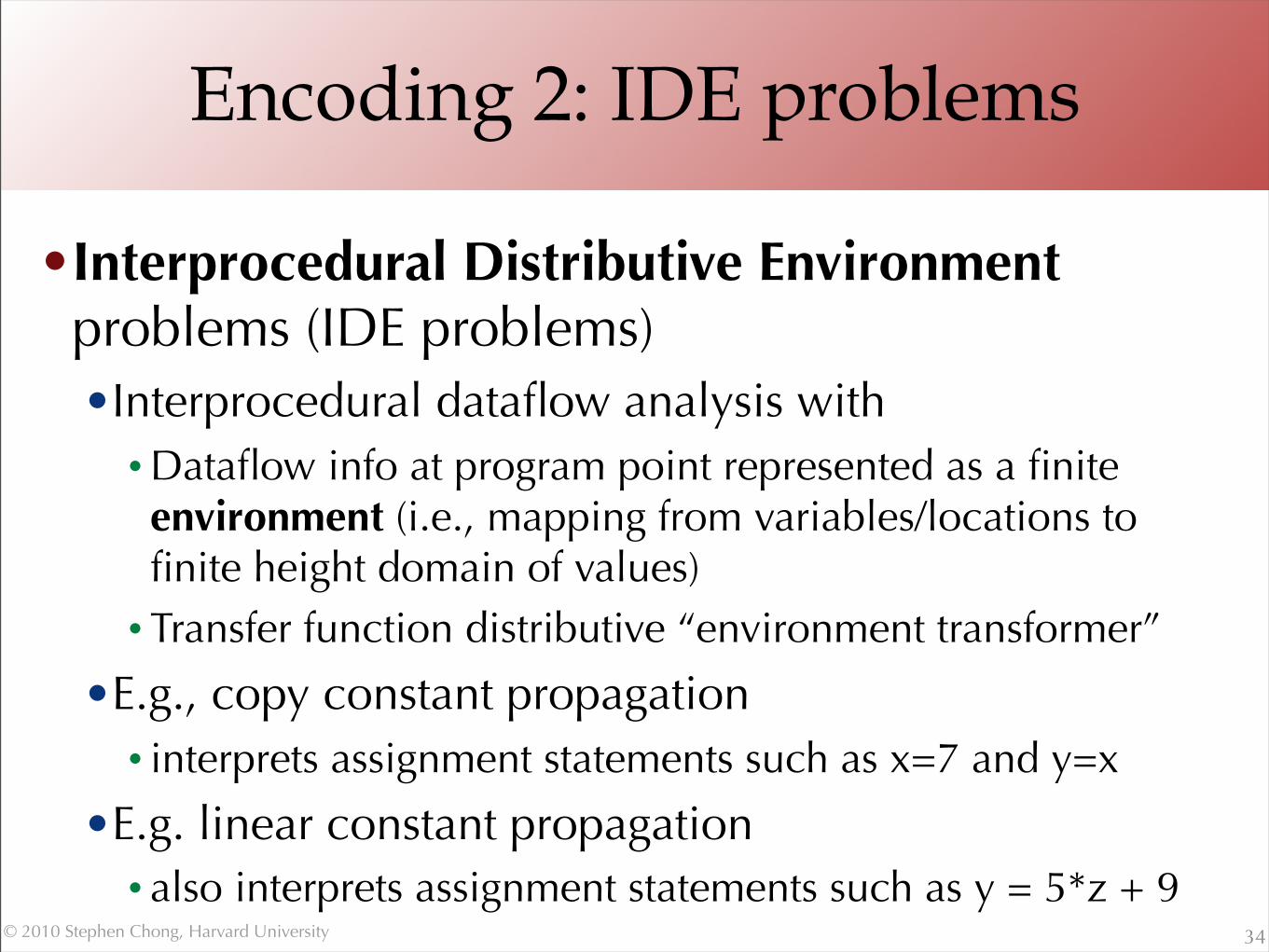
Encoding 2: IDE problems
•Interprocedural Distributive Environment problems (IDE problems)•Interprocedural dataflow analysis with•Dataflow info at program point represented as a finite environment (i.e., mapping from variables/locations to finite height domain of values)• Transfer function distributive “environment transformer”
•E.g., copy constant propagation• interprets assignment statements such as x=7 and y=x
•E.g. linear constant propagation• also interprets assignment statements such as y = 5*z + 9
34
© 2010 Stephen Chong, Harvard University
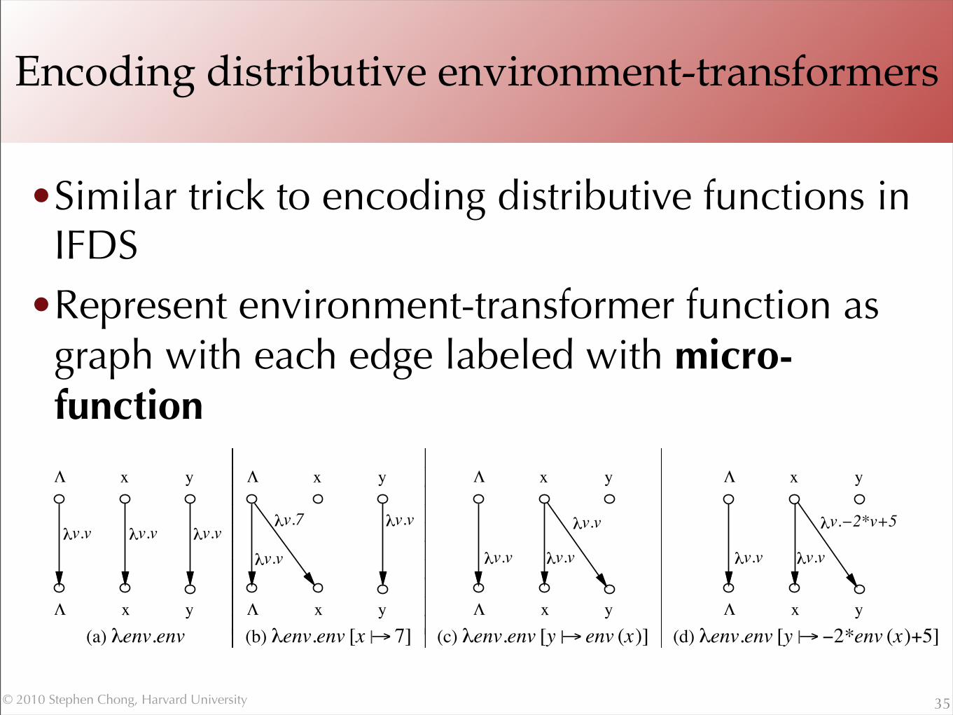
Encoding distributive environment-transformers
•Similar trick to encoding distributive functions in IFDS
•Represent environment-transformer function as graph with each edge labeled with micro-function
35
! 23 !
O ((P " E) + (CallSites " Params 2)).This approach is used in the Wisconsin Program-Slicing Tool, a slicing system that supports essentially
the full C language. (The system is available under license from the University of Wisconsin. It has beensuccessfully applied to slice programs as large as 51,000 lines.)
6. Program Analysis Using More Than Graph ReachabilityThe graph-reachability approach offers insight into ways that machinery more powerful than the graph-reachability techniques described above can be brought to bear on program-analysis problems [78,88].One way to generalize the CFL-reachability approach stems from the observation that CFL-reachability
problems correspond to chain programs, which are a restricted class of Datalog programs. The fact thatCFL-reachability problems are related to chain programs, together with the fact that chain programs arejust a special case of the logic programs to which tabulation and transformation techniques apply, suggeststhat more powerful program-analysis algorithms can be obtained by going outside the class of pure chainprograms [78].A different way to generalize the CFL-reachability approach so as to bring more powerful techniques to
bear on interprocedural dataflow analysis was presented in [88]. This method applies to problems in whichthe dataflow information at a program point is represented by a finite environment (i.e., a mapping from afinite set of symbols to a finite-height domain of values), and the effect of a program operation is capturedby a distributive “environment-transformer” function. This class of dataflow problems has been called theInterprocedural Distributive Environment problems (or IDE problems, for short).Two of the dataflow-analysis problems that the IDE framework handles are (decidable) variants of the
constant-propagation problem: copy-constant propagation and linear-constant propagation. The formerinterprets assignment statements of the form x = 7 and y = x. The latter also interprets statements of theform y = !2*x +5.By means of an “explosion transformation” similar to the one utilized in Section 4.1, an interprocedural
distributive-environment-transformer problem can be transformed from a meet-over-all-realizable-pathsproblem on a program’s supergraph to a meet-over-all-realizable-paths problem on a graph that is larger,but in which every edge is labeled with a much simpler edge function (a so-called “micro-function”) [88].Each micro-function on an edge d 1 # d 2 captures the effect that the value of symbol d 1 in the argumentenvironment has on the value of symbol d 2 in the result environment. Fig. 10 shows the explodedrepresentations of four environment-transformer functions used in constant propagation. Fig. 10(a) showshow the identity function $env.env is represented. Figs. 10(b)!(d) show the representations of the func-tions $env.env [x ||# 7], $env.env [y ||# env (x)], and $env.env [y ||#!2*env (x)+5], which are the dataflowfunctions for the statements x = 7, y = x, and y = !2*x +5, respectively. (% is used to represent the effectsof a function that are independent of the argument environment. Each graph includes an edge of the form%#%, labeled with $v.v; as in Section 4.1, these edges are needed to capture function composition prop-erly.)Dynamic programming on the exploded supergraph can be used to find the meet-over-all-realizable-
paths solution to the original problem: An exhaustive algorithm can be used to find the values for all sym-bols at all program points; a demand algorithm can be used to find the value for an individual symbol at a
%
%
v.v$v.v$v.v$
x y
x y
%
%
v.v$
v.v$$v.7
x y
x y
%
%
v.v$ v.v$
x y
x y
v.v$
%
%
v.v$
$v.!2*v+5
v.v$
x y
x y(a) $env.env (b) $env.env [x ||# 7] (c) $env.env [y ||# env (x)] (d) $env.env [y ||#!2*env (x)+5]
Fig. 10. The exploded representations of four environment-transformer functions used in constant propagation.

© 2010 Stephen Chong, Harvard University
Solving
•Requirements for class F of micro functions•Must be closed under meet and composition
•F must have finite height (under pointwise ordering)
•f(l) can be computed in constant time
•Representation of f is of bounded size
•Given representation of f1, f2 ∈ F• can compute representation of f1 ○ f2 ∈ F in constant time
• can compute representation of f1 ⊓ f2 ∈ F in constant time
• can compute f1 = f2 in constant time
36
© 2010 Stephen Chong, Harvard University
Solving
•First pass computes jump functions and summary functions•Summaries of paths within a procedure and of
procedure calls, respectively
•Second pass uses these functions to computer environments at program points
•More details in “Precise Interprocedural Dataflow Analysis with Applications to Constant Propagation” by Sagiv, Reps, and Horwitz, 1996.
37