Quality of Service Analysis and Control for Wireless Sensor Networks

James Kay and Jeff Frolik

University of Vermont

jkay@uvm.edu, jfrolik@emba.uvm.edu

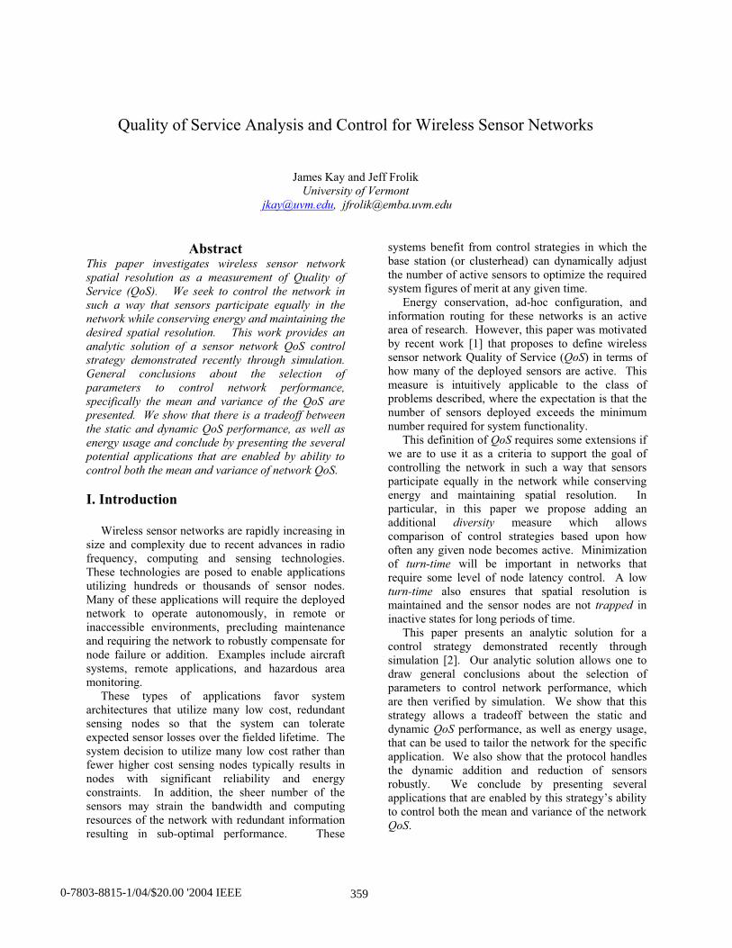
AbstractThis paper investigates wireless sensor network

spatial resolution as a measurement of Quality of

Service (QoS). We seek to control the network in such a way that sensors participate equally in the

network while conserving energy and maintaining thedesired spatial resolution. This work provides an

analytic solution of a sensor network QoS control

strategy demonstrated recently through simulation.General conclusions about the selection of

parameters to control network performance,

specifically the mean and variance of the QoS are presented. We show that there is a tradeoff between

the static and dynamic QoS performance, as well as

energy usage and conclude by presenting the several potential applications that are enabled by ability to

control both the mean and variance of network QoS.

I. Introduction

Wireless sensor networks are rapidly increasing in

size and complexity due to recent advances in radio

frequency, computing and sensing technologies.

These technologies are posed to enable applications

utilizing hundreds or thousands of sensor nodes.

Many of these applications will require the deployed

network to operate autonomously, in remote or

inaccessible environments, precluding maintenance

and requiring the network to robustly compensate for

node failure or addition. Examples include aircraft

systems, remote applications, and hazardous area

monitoring.

These types of applications favor system

architectures that utilize many low cost, redundant

sensing nodes so that the system can tolerate

expected sensor losses over the fielded lifetime. The

system decision to utilize many low cost rather than

fewer higher cost sensing nodes typically results in

nodes with significant reliability and energy

constraints. In addition, the sheer number of the

sensors may strain the bandwidth and computing

resources of the network with redundant information

resulting in sub-optimal performance. These

systems benefit from control strategies in which the

base station (or clusterhead) can dynamically adjust

the number of active sensors to optimize the required

system figures of merit at any given time.

Energy conservation, ad-hoc configuration, and

information routing for these networks is an active

area of research. However, this paper was motivated

by recent work [1] that proposes to define wireless

sensor network Quality of Service (QoS) in terms of

how many of the deployed sensors are active. This

measure is intuitively applicable to the class of

problems described, where the expectation is that the

number of sensors deployed exceeds the minimum

number required for system functionality.

This definition of QoS requires some extensions if

we are to use it as a criteria to support the goal of

controlling the network in such a way that sensors

participate equally in the network while conserving

energy and maintaining spatial resolution. In

particular, in this paper we propose adding an

additional diversity measure which allows

comparison of control strategies based upon how

often any given node becomes active. Minimization

of turn-time will be important in networks that

require some level of node latency control. A low

turn-time also ensures that spatial resolution is

maintained and the sensor nodes are not trapped in

inactive states for long periods of time.

This paper presents an analytic solution for a

control strategy demonstrated recently through

simulation [2]. Our analytic solution allows one to

draw general conclusions about the selection of

parameters to control network performance, which

are then verified by simulation. We show that this

strategy allows a tradeoff between the static and

dynamic QoS performance, as well as energy usage,

that can be used to tailor the network for the specific

application. We also show that the protocol handles

the dynamic addition and reduction of sensors

robustly. We conclude by presenting several

applications that are enabled by this strategy’s ability

to control both the mean and variance of the network

QoS.

3590-7803-8815-1/04/$20.00 '2004 IEEE

The remainder of this paper is organized as

follows: Section II presents the control architecture

investigated in this paper and discusses previous

results. Section III presents an analysis of this

architecture using Markov processes. A direct

formulation of the problem is presented first,

followed by a formulation that significantly reduces

the dimensionality of the problem. Section IV

presents the key results of using this analysis, and

simulation. We conclude in Section V with proposed

extensions to this work.

II. Sensor Automaton and Control

Strategies

This work was motivated by two recently

presented QoS control strategies. Again, we consider

QoS as being defined in terms of average spatial

resolution or equivalently the number of sensors

active in a randomly deployed network. Specifically

we consider the Gur strategy proposed in [1,3] and

the ACK strategy proposed in [2]. Both of these

strategies control QoS for a single-hop cluster. In

addition, both strategies have sensors that use finite

state automata. We will briefly discuss both

strategies to give the reader an appreciation for the

differences and similarities of these techniques. This

will be followed by a detailed analysis of the ACK

strategy.

In the following description we will denote the

number of sensor nodes by N, and the number of

possible node automaton states by G. We distinguish

between the state of each automata and the state of

the entire network by using the terms automata state

and system state.

In both techniques one sensor is active as the

clusterhead node. This sensor receives information

from all other sensors in the network. It is assumed

that all sensors have sufficient transmission strength

to cover the entire area (i.e. cluster). These

techniques are applicable to a wide range of networks

including band limited applications suitable for low-

cost monitoring (e.g. environmental), as well as high

bandwidth applications (e.g. target tracking). This

makes this technique compatible with various

communication protocols including low cost

ALOHA, and carrier sense multiple access (CSMA)

methods.

A. Gur Game

In the Gur strategy the remaining sensors are in

either a STANDBY or ON state as shown in Fig. 1.

Sensors in the ON state are active in sending data to

the clusterhead and counted to determine the network

QoS. Sensors in the STANDBY state do not send

data.

REWARD

-3 -2 -1 1 2 3

PUNISHMENT

STANDBY ON

Figure 1. Gur game automaton.

Sensors move from one state to another based on

being rewarded for their behavior (ON or

STANDBY). Each sensor determines whether to

reward or punish itself based upon a threshold, R,

between 0 and 1 received from the clusterhead. Each

node locally generates a random number, between 0

and 1, and rewards itself if this number is less than R,

otherwise the node punishes itself. The value of R is

calculated once each epoch by the clusterhead and

broadcasted to all sensors, including those in the

STANDBY state.

The threshold R is calculated from a function

whose domain is the QoS calculated above and

whose range is 0 to 1. [1,3] have shown that for this

architecture the mean of the resulting QoS will tend

to the maximum of this reward function for a very

broad class of functions, allowing control of the

network QoS. However, expressions for second and

higher order statistics for this technique have not

been calculated.

The Gur control strategy has two parameters that

can be used to control the network performance, the

number of automata states, and the particular form of

the reward function. [1,3] have shown that 3 ON and

3 STANDBY states provide adequate control. We

are unaware of work on selection of the reward

function to optimize the dynamics (e.g. settling time,

stability, and variance) of the QoS.

B. ACK Automaton.

The ACK protocol was developed as an

alternative to the Gur game [2]. In this technique,

rather than automata states being ON or STANDBY

they are in varying states of being ON. This is

accomplished by assigning a transmit probability Ti

to each of the automata states. During each epoch,

each sensor independently generates a random

360

number between 0 and 1. If this number is less than

Ti, the node transmits, otherwise it is silent. The

clusterhead acknowledges each transmitting sensor

individually and provides a single bit of coupling

information indicating whether the current QoS is

greater than the desired value, Q0. Sensors

transition between states based on this single bit of

information. They punish themselves if the QoS is

greater than the desired value by transitioning toward

the left in Fig. 2. Conversely they reward themselves

by moving right if the QoS is less than or equal to the

desired value. Note that in this technique sensors that

do not transmit can be in a very low power state since

they do not need to listen for control information

from the clusterhead.

desired value. Note that in this technique sensors that

do not transmit can be in a very low power state since

they do not need to listen for control information

from the clusterhead.

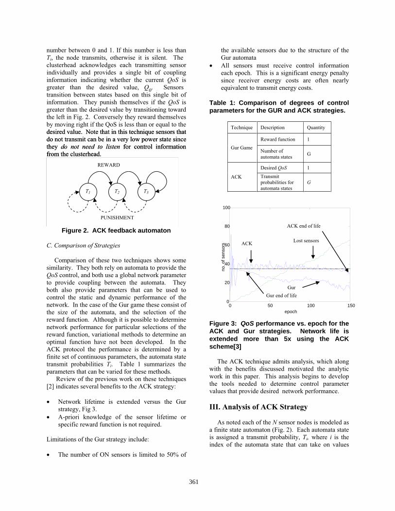
Figure 2. ACK feedback automaton

C. Comparison of Strategies

Comparison of these two techniques shows some

similarity. They both rely on automata to provide the

QoS control, and both use a global network parameter

to provide coupling between the automata. They

both also provide parameters that can be used to

control the static and dynamic performance of the

network. In the case of the Gur game these consist of

the size of the automata, and the selection of the

reward function. Although it is possible to determine

network performance for particular selections of the

reward function, variational methods to determine an

optimal function have not been developed. In the

ACK protocol the performance is determined by a

finite set of continuous parameters, the automata state

transmit probabilities Ti. Table 1 summarizes the

parameters that can be varied for these methods.

Review of the previous work on these techniques

[2] indicates several benefits to the ACK strategy:

Network lifetime is extended versus the Gur

strategy, Fig 3.

A-priori knowledge of the sensor lifetime or

specific reward function is not required.

Limitations of the Gur strategy include:

The number of ON sensors is limited to 50% of

the available sensors due to the structure of the

Gur automata

All sensors must receive control information

each epoch. This is a significant energy penalty

since receiver energy costs are often nearly

equivalent to transmit energy costs.

Table 1: Comparison of degrees of controlparameters for the GUR and ACK strategies.

Technique Description Quantity

Reward function 1

Gur GameNumber of

automata states G

Desired QoS 1

ACK Transmit

probabilities for

automata states

G

REWARD

T2 T3T1

no.o

fsen

sors

100

PUNISHMENT

ACK end of life 80

ACK

Gur

Lost sensors

40

60

20

Gur end of life

Figure 3: QoS performance vs. epoch for theACK and Gur strategies. Network life is extended more than 5x using the ACK scheme[3]

The ACK technique admits analysis, which along

with the benefits discussed motivated the analytic

work in this paper. This analysis begins to develop

the tools needed to determine control parameter

values that provide desired network performance.

III. Analysis of ACK Strategy

As noted each of the N sensor nodes is modeled as

a finite state automaton (Fig. 2). Each automata state

is assigned a transmit probability, Ti, where i is the

index of the automata state that can take on values

00

10050 150epoch

361

from 1 to G. Therefore, in any epoch a sensor node in

automata state i has probability Ti of transmitting.

A. State Transition Rules

The N sensors in the network receive an

acknowledgement (ACK) when they transmit. This

single bit of information provides the only coupling

of the global network state to the individual automata

state. In the proposed QoS control strategy transitions

between automata states are controlled by the

following rules:

Rule 1: A transmitting node goes to the next higher

automata state if QoS Q0. If a transmitting node is

already in the highest automata state, it remains in the

highest state.

Rule 2: A transmitting node goes to the next lower

automata state if QoS>Q0. If a transmitting node is

already in the lowest automata state, it remains in the

lowest state.

Rule 3: Non-transmitting nodes do not change

automata states.

These rules along with the automata structure

allow modeling the network as a Markov process for

which steady state and dynamic solution techniques

are well known[4,5]. Note that the transition

probabilities are functions of the global network

parameter Q0 which prevents modeling each node

independently of the others.

Figure 4: State enumeration, top is direct method, bottom is condensed method. Theexample shown is for 5 nodes, each with 3automaton states.

B. Direct Markov Modeling of System

The assignment of the Markov states for this

formulation is shown in the top half of Fig. 4. The

states are enumerated by N transmit digits and Nautomata state digits. The transmit digits will always

be binary digits, while the base of the automata state

digits will be equal to G, the number of automata

states. This assignment results in 2NGN states.

Examination of this state assignment shows that

every combination of automata state and network

state can be represented. For example, Fig. 4 shows

the case when we have five nodes (N=5) and 3

automaton states (G=3). In the specific network state

shown nodes 3 and 4 are transmitting, and the other

nodes are not. In addition we see that nodes 1 and 5

are in automaton state 3, nodes 2 and 3 are in

automaton state 1, and node 4 is in automaton state 2.

This state enumeration provides knowledge of the

network QoS (the sum of the Transmit Digits) as well

as the automaton state of each node. It is

straightforward to calculate the probability of

transitioning from any state, to any other state using

the following rules. We use Sj to designate the

current network state (i.e. the combination of the

transmit digits and the automaton digits) and Si to

designate the next state of the system. Using this

notation the Markov state transition probabilities

between any two states can be calculated using the

following two step process:

Step 1: Determine which transitions have non-zero

probabilities.

i. If a node’s transmit digit is 0, then it remains in its

current automaton state, since it will not receive any

ACK information from the BASE. Any network

state transition for which this is not true has 0

probability.N Transmit Digits N Automata State Digits ii. If a node’s transmit digit is 1, the automaton state

for that node is increased by 1 if the sum of the

transmit digits in state Si Q0 (reward), and decreased

by 1 if Si>Q0 (punish). Exceptions to this rule occur

at the end states (i.e. when the automaton state is

either 1 or G). If a node is in the 1 state and is

punished, it remains in the 1 state. Similarly if a

node is in automaton state G and is rewarded it

remains in state G. Any network state transition for

which this rule is not followed has 0 probability.

1

1

G

GN)2( NN G

0 0 1 1 0 3 1 1 2 3

Base 2 Base ‘G’

2 1 2 States using

the condensed

methodStates using

the direct

method

Number of nodes in each

automaton state

Step 2: Determine the transition probabilities for the

non-zero cases.

i. The transition probability between Sj and Si is a

product consisting of N terms, one for each node. To

determine the term corresponding to a node first

identify for state Si, the automaton state, k for that

node, and the transmit state for that node. If the

transmit state for a node is 1, then choose the transmit

probability, Tk for the product term for that node. If

362

the transmit state for a node is 0, choose 1-Tk for the

product term.

The results for the mean and variance of QoS for

this case are shown in Fig. 6. In the top figure the

height of the surface is the expected value of QoS.

We have highlighted that region for which |E(QoS)-

Q0|<0.01 by setting the surface height to 0 in this case

(as indicated by the arrow). We also plot the

variance of QoS as a function of T1 and T2 along this

highlighted region, in the lower half of Fig. 6.

The results for the mean and variance of QoS for

this case are shown in Fig. 6. In the top figure the

height of the surface is the expected value of QoS.

We have highlighted that region for which |E(QoS)-

Q0|<0.01 by setting the surface height to 0 in this case

(as indicated by the arrow). We also plot the

variance of QoS as a function of T1 and T2 along this

highlighted region, in the lower half of Fig. 6.

Sj=

Si=

Figure 5: Network states Si and Sj, for N=5,G=3, Q0=3

1 1 0 0 0 1 2 1 1 1

1 0 0 1 1 2 3 1 1 1

Variance

T1

T2

To illustrate the calculation of transitional

probabilities consider the example of Fig. 5 where we

assume Q0=3. In this case, the transition from Sj to Si

will be a reward transition, since the QoS of Sj is 2

which is less than or equal to Q0. We also apply step

1 and determine that the transition probability is not

0. We then form the expression for the transition

probability between states Sj and Si which we denote

Pji as:

To illustrate the calculation of transitional

probabilities consider the example of Fig. 5 where we

assume Q0=3. In this case, the transition from Sj to Si

will be a reward transition, since the QoS of Sj is 2

which is less than or equal to Q0. We also apply step

1 and determine that the transition probability is not

0. We then form the expression for the transition

probability between states Sj and Si which we denote

Pji as:

Pji=T2Q3Q1T1T1 (1)Pji=T2Q3Q1T1T1 (1)

Where Q3=1-T3, Q1=1-T1.Where Q3=1-T3, Q1=1-T1.

Once the transition probabilities between each

state are determined the solution for the probability

of the network being in any state Si, which we denote

P(Si) can be determined using standard Markov

process solution techniques, e.g. [4,5]. Since the QoS

of each Si is known we can then determine the

probability distribution function for the random

variable QoS by weighting each value of QoS by the

sum of the state probabilities for all states with that

value of QoS.

Once the transition probabilities between each

state are determined the solution for the probability

of the network being in any state Si, which we denote

P(Si) can be determined using standard Markov

process solution techniques, e.g. [4,5]. Since the QoS

of each Si is known we can then determine the

probability distribution function for the random

variable QoS by weighting each value of QoS by the

sum of the state probabilities for all states with that

value of QoS.

Figure 6: Results for N=2 G=2, Q0=1

Observations from Fig. 6 are:

1. When T1=T2=0.5 the expected value is exactly 1,

and the variance is exactly 0.5. In this case, G really

is reduced from 2 to 1 since the probability of

transmit does not depend on the automaton state of

that node. In this case we have a Bernoulli process

[2] and we may write the mean and variance as:

The analysis above is valid when Q0<N, and when

all the Ti>0, in which case the process is completely

ergodic and therefore has limiting state probabilities

[4], and can be solved analytically for the probability

density function (pdf) of QoS for each value of N and

G. Knowledge of the pdf allows the calculation of

any statistical moment for QoS. Results for N=2,

G=2 and Q0=1 are given in (2), where we use a

normalizing factor, D, to simplify the expression.

The analysis above is valid when Q0<N, and when

all the Ti>0, in which case the process is completely

ergodic and therefore has limiting state probabilities

[4], and can be solved analytically for the probability

density function (pdf) of QoS for each value of N and

G. Knowledge of the pdf allows the calculation of

any statistical moment for QoS. Results for N=2,

G=2 and Q0=1 are given in (2), where we use a

normalizing factor, D, to simplify the expression.

5.0)5.01(5.02)1()(

15.02)(

TNTQoSVar

NTQoSE (3)

This result is consistent with Fig. 6.

2. Along the curve for which E(QoS)=Q0=1 the

minimum variance occurs when T2=1,

2221

1T , and has value 414.012

which is less than the case of G=1 for which the

variance is 0.5 Results will be presented later in this

paper showing additional control of the variance as

we increase G.

)1(23)1(2

)2(/)2()2(

)2(/)22

4444()1(

)2(/)223

36622()0(

2221

222

21

22

21

221

321

32

22

21

2212

2121

321

32

22

21

222

2121

211

TTTTTTDwhere

cDTTTTQoSP

bDTTT

TTTTTTTTQoSP

aDTTTTT

TTTTTTTQoSP

)1(23)1(2

)2(/)2()2(

)2(/)22

4444()1(

)2(/)223

36622()0(

2221

222

21

22

21

221

321

32

22

21

2212

2121

321

32

22

21

222

2121

211

TTTTTTDwhere

cDTTTTQoSP

bDTTT

TTTTTTTTQoSP

aDTTTTT

TTTTTTTQoSP

Although we now have an analytic solution for the

network, its usefulness is limited. It suffers from the

curse of dimensionality, since the number of states

363

grows as 2NGN. Even for a simple network consisting

of two nodes with two automata states we must solve

a set of sixteen linear equations.

iS =The event that the network transitions to

network state Si.

In equation (4) the P(Si) are unknowns. The

remaining conditional probabilities, ’s, are

known given the transition rules presented earlier. It

is convenient to define an activity measure between

automaton states to facilitate writing an analytic

expression for the ’s. We define:

)/( ji SSP

)/( ji SSP

C. Reducing Analytic Complexity

This rapid state growth in the formulation above

provides motivation for reformulating the problem in

a way that significantly reduces the number of states.

Our approach is to rewrite the system equations in

terms of conditional probabilities. In the previous

formulation we noted that there are GN distinct

automaton states in the Markov process. However,

due to symmetry, network states with the equal

numbers of nodes in each automaton state will have

the same limiting state probabilities and can be

represented as a single state. This results in

Ak(Si,Sj) = The number of nodes in the k’th digit of

the state vector Sj that must transmit in order for

the network to transition to state Si.

The domain of Ak(Si,Sj) is defined to be those

ordered pairs of states, (Si,Sj) which are consistent

with the state transition rules presented earlier, and

for which i j. Those transitions that do not obey

these rules have 0 probability of occurrence, and we

treat the case of i=j as a special case. The domain of

Ak can be further divided into pairs representing

reward, and punish transitions. We designate these

subdomains as Dr, Dp respectively. Due to the hard

limiting of rewarding and punishing at the G’th and

1’st automaton states we leave Ak(Si,Sj) undefined

when k=G for reward states and k=1 for punishstates. We provide an example showing Si, Sj, and Ak

for a reward transition in Fig. 7, for a network with 6

automata states. As discussed above Ak is not defined

for k=6 in this case.

C =1

1

G

GN

unique automaton states (see Fig. 4). A comparison

of the dimensionality for the two formulations is

shown in Table 2, and provides motivation for

condensing the states.

Table 2: Comparison of Markov states forthe direct and condensed formulations

Markov States N G

Direct Condensed

2 2 16 3

3 3 216 10

4 3 1296 15

7 3 2.8E3 36

8 3 1.67E6 45

20 3 3.6E15 231

k= 1 2 3 4 5 6

Sj = 2 1 2 4 1 0

Si= 1 1 3 3 1 1

Ak= 1 1 2 1 1 X We represent these state probabilities by P(Si)

where the subscript takes on C values. These state

probabilities obey the following equation:Figure 7: Example calculation for Ak

Using these definitions we may rewrite (4) as: )()/()( jj

j

ii SPSSPSP (4)

)()/(

)()/()()/()(

),(),(

iii

jj

DSS

ijj

DSS

ii

SPSSP

SPSSPSPSSPSPp

jir

ji

where:

Si=The event that the network is in automaton

state i. We order the G digits of this network

state from 1 to G, with the G’th digit containing

the number of network nodes in the highest

reward state, G-1 the next highest reward state,

down to 1, which is the lowest, most punished

state. The bottom half of Fig. 4 illustrates the case

of 5 nodes, with 2 in the lowest state, 1 in the

second state, and 2 in the highest state.

(5)

This partitioning allows modeling each of the

conditional probabilities in (4) as a set of independent

Bernoulli processes. This independence allows us to express these probabilities as the product of the

probabilities of the independent processes. We

364

define the following notation for the Bernoulli pdf

and cumulative distribution function (cdf):

(6-8) are explained by reference to the activity

measure, Ak. Consider the reward case (7),

(i.e. ). We wish to determine the

conditional probability of transition from state S

rji DSS ),(

kjS

(b

j to

Si. For this transition to occur, we require a specific number of the total number of sensors in each of the

G automaton states to transmit. The number required

to transmit in the k’th automaton state is Ak(Si,Sj).Since the total number of sensors in the k’th

automaton is , the probability that Ak(Si,Sj) of them

will transmit is .),);,( kkjjik TSSSA

wnw ppw

npnwb )1(),;(

= the probability of w successes in nindependent Bernoulli trials with successprobability p. If n=0 we define b(w;n,p)=1when w=0, and 0 elsewhere. If w<0 we define

b(w;n,p)=0.w

i

pnibpnwB

0

),;(),;(

= the probability of w or fewer successes in nindependent Bernoulli trials with success

probability p. If w<0 we define B(w;n,p)=0.

For a given Si, the number of sensors transmitting

in each automaton state is only a function of the

number of sensors in that state. This independenceallows determination of the total probability of

transition as the product of the individualprobabilities, which is represented by the product

term of (7). A special case occurs at automaton state

G for the reward case and state 1 for the punish case. The number of sensors transmitting in these limiting

(i.e. k=1 or G) states is not unique for all transitions,

which is why Ak is left undefined for these cases. Inthe case of a reward transition the number

transmitting in the G’th automaton state, plus the sum

of the sensors transmitting in the other states must be less than or equal to Q0. The probability of this

occurring is: .),);,((

1

1

0 GGjji

G

k

k TSSSAQB

In addition we define:miS = the value of the m’th digit of the state Si.

Referring to the lower half of Fig. 4, we see:1. Digits can range in value from 0 to N.

2. There are G digits in each network state Si,.

3. The value of m can range from 1 to G.

4. for each value of iNS

G

m

mi

1

We now formulate the conditional probabilities as:

If ( (punish case):pji DSS ),

In the case where i=j we require that only sensors

in the limiting states can transmit. The first term in

(8) accounts for the punish case, where only sensors in state 1 are allowed to transmit. The second term

accounts for the reward case, where only sensors in

state G are allowed to transmit.(6))6(),);,((

)},);,((1{)/(

2

11

2

0

m

G

m

mjjim

jj

G

k

ikji

TSSSAb

TSSSAQBSSP

We now have a set of C linear equations for the Cunknown P(Si)’s. These determine the P(Si)’s to a multiplicative constant [4]. We add the additional

constraint that the state probabilities must sum to 1,

i.e.

If (reward case):rDSS ),( ji

)7(),);,((

),);,(()/(

1

1

1

0

m

Gmjjim

GGjj

G

k

ik

ji

TSSSAb

TSSSAQBSSP

1m

i

iSP 1)(

We now derive the probability density function for

QoS given these P(Si)’s. This pdf can then be used to

calculate desired QoS statistics, in particular themean and variance.If i=j (special case):

)8(),;0(),;(

),;0()},;(1{)/(

1

0

2

11

0

m

GmiG

Gi

m

G

m

miiji

TSbTSQB

TSbTSQBSSP

1m

E. Calculation of the Probability Distribution Function for QoS

Given the P(Si) we may write the pdf of QoS as asum of conditional probabilities as follows:

365

)()/()( i

S

i SPSxQoSPxQoSP

i

(9)selecting T1. This allow

performance to the applica

We now define:

)(xf ki ),;( k

ki TSxb

= the probability that x of the nodes in

automaton state k of network state Si are

transmitting.

The f defined above are independent of each other

and can each be viewed as the pdf of a randomvariable x. The sum of these random variables for a

given network state is the QoS for that network state.

The pdf of the sum of independent random variablesis the convolution of their pdf’s [2]. Therefore the

pdf of QoS may be written as the discrete convolution

of these independent pdf’s giving:

and can each be viewed as the pdf of a randomvariable x. The sum of these random variables for a

given network state is the QoS for that network state.

The pdf of the sum of independent random variablesis the convolution of their pdf’s [2]. Therefore the

pdf of QoS may be written as the discrete convolution

of these independent pdf’s giving:

G

iiiii ffffSxQoSP ...)/( 321 Giiiii ffffSxQoSP ...)/( 321 (10) (10)

Given we can determine the pdf of QoS, any

statistical moment can be calculated, in particular the

mean and variance.

Given we can determine the pdf of QoS, anystatistical moment can be calculated, in particular the

mean and variance.

IV. Key Results IV. Key Results

Investigations of our analysis have yielded several

key results.

Investigations of our analysis have yielded several

key results.

Result 1. The mean and variance of QoS can becontrolled by selection of the transmit probabilities.Result 1. The mean and variance of QoS can becontrolled by selection of the transmit probabilities.

An example is shown in Fig. 8 for the case when

N=5, G=3, Q0=3. In this example we have set T3=1

and allowed T2 and T1 to vary. In the left hand plotwe have highlighted the region for which |E(QoS)-

Q0|<0.03 in black. There are actually two curves for

which this condition holds, the first is the easily seen funnel shaped curve, the second one is a narrow strip

that occurs when T1 approaches 0 (as indicated by the

arrow). Note that the funnel mouth widens as T2

approaches 1. This feature allows control of the

variance while maintaining a mean near the control

point. We illustrate this in the right hand side of Fig.8, where we fix T2 at 0.8, and keep T3=1.0, while we

vary T1 to control the variance. By allowing T1 to vary from 0 to 0.45 we can choose a variance

between 0 and 1.2. This ability to control the

variance while keeping the mean relatively constantwas observed in all cases analyzed. In the case of

G=3 the range over which the variance can be

controlled can be set by appropriate selection of T2,and the operating point for the variance controlled by

s tuning the network

tion. Wider ranges ofmean and variance control are possible as we

increase the network size, N, and the number of

automaton states, G.

An example is shown in Fig. 8 for the case when

N=5, G=3, Q0=3. In this example we have set T3=1

and allowed T2 and T1 to vary. In the left hand plotwe have highlighted the region for which |E(QoS)-

Q0|<0.03 in black. There are actually two curves for

which this condition holds, the first is the easily seen funnel shaped curve, the second one is a narrow strip

that occurs when T1 approaches 0 (as indicated by the

arrow). Note that the funnel mouth widens as T2

approaches 1. This feature allows control of the

variance while maintaining a mean near the control

point. We illustrate this in the right hand side of Fig.8, where we fix T2 at 0.8, and keep T3=1.0, while we

vary T1 to control the variance. By allowing T1 to vary from 0 to 0.45 we can choose a variance

between 0 and 1.2. This ability to control the

variance while keeping the mean relatively constantwas observed in all cases analyzed. In the case of

G=3 the range over which the variance can be

controlled can be set by appropriate selection of T2,and the operating point for the variance controlled by

selecting T1. This allows tuning the network

performance to the application. Wider ranges ofmean and variance control are possible as we

increase the network size, N, and the number of

automaton states, G.

0 0.2 0.4 0.6 0.8 10

0.2

0.4

0.6

0.8

1

0 0.2 0.4 0.6 0.8 10

1

2

3

4

53 p2=0.8 p3=1.0

E(QoS)Var(Qos)

T2=0.8 T3=1.0N=5 G=3 Q0=3 T3=1.0

T1

T2 T1

Figure 8. Mean and variance as a function ofthe transmit probabilities.

Result 2. There is a tradeoff between variance andnetwork diversity.

We define diversity loosely as equality of

participation among sensors. We will develop thisconcept by briefly revisiting our analysis, followed

by the introduction of a more formal diversity

measure we name turn time.One of the results of condensing the number of

Markov states is that we lose individual nodeinformation, while retaining network level

information. Thus, our solution allows calculation of

all statistics for the QoS, but does not allow us to determine the specific performance of any individual

node. The result is that systems designed using the

QoS analysis alone may behave in undesired ways.This is illustrated by using the example of N=5,

G=3, and Q0=3 presented in Fig. 8. Let’s assume our

task is to design the system with the minimumvariance in the QoS, while maintaining the mean

close to Q0=3. Using Fig. 8, we decide to select

T1=0, T2=0.8, and T3=1.0. For this selection we seethat the mean is 3.0 and the variance is 0. We met

our goals perfectly! The issue is that the network has

a low diversity. For this particular selection of Ti’swe can analyze the solution in closed form and see

that in this case 3 of the nodes will eventually reach

the highest automaton state and 2 will eventuallyreach the lowest automaton state. Once the network

reaches this configuration no additional automatonstate transitions will occur thus each sensor is

trapped into its final state and some will nottransmit. The specific sensors trapped in this lowest state will depend upon the starting state of the

network, and how it evolves based on the stochastic

rules presented earlier. Note that this trappingbehavior occurs anytime we set the lowest

366

automaton’s transmit probability to 0. The problem

arises should one of the transmitting nodes fail, thuscausing the QoS to drop to 2 without possibility of

achieving Q0 subsequently. (Note that our original

analysis specifically excluded this case, although it is valid for values arbitrarily close to 0).

0 500 1000 1500 2000 2500 3000 3500 4000 4500 50000

200

400

600

800

1000

1200

1400

1600

1800

2000

Turn Time (epochs)

Fre

quen

cy(C

ount

s)

N=4 Q0=3 T1=0.1 T2=0.5 T3=1 T4=1

E(QoS)=3.06 Var(QoS)=0.16

Frequency

(Counts)The discussion above begs the question of how to

trade off variance for diversity in this QoS control strategy. We propose introducing a metric for

diversity measure, turn time, defined as the time,

measured in network epochs, that it takes a sensor inthe network to transition from the lowest automaton

state to the highest automaton state. Turn time beinga random variable can be described by its statistics.

However, the condensed problem formulation trades

off dimensionality for granularity, and cannotdistinguish individual sensor performance. Therefore

simulation of the network is used to obtain turn timestatistics.

Figure 9: Turn time for N=4, Q0=3, T1=0.1,T2=0.5, T3=1, T4=1

0 1 2 3 4 5 6 7

x 105

0

0.5

1

1.5

2

2.5

3

Turn Time (epochs)

Fre

quen

cy(c

ount

s)

N=4 Q0=3 T1=0.01 T2=0.5 T3=1 T4=1E(QoS)=3.01 Var(QoS)=0.012Fig. 9 and Fig. 10 illustrate the tradeoff between

variance and turn time. The two cases are identical

except for the value of T1 which is 0.1 in Fig. 9, and0.01 in Fig. 10. Both cases maintain the mean of

QoS near the desired control point of Q0=3. The

variance in Fig. 9 is ~10 times greater than that in Fig. 10, but is still relatively small (~5% of the

mean). However, the two networks have widely

different turn times. Note that the scale on Fig. 10 is multiplied by 105. The simulation for Fig. 10 was

run with 106 epochs, and still only had a total of 6

turns in the entire simulation. The network of Fig. 10would respond extremely slowly to sensor failures.

Frequency

(Counts)

Figure 10: Turn time for N=4, Q0=3, T1=0.01,T2=0.5, T3=1, T4=1

We conclude discussion of this result byreiterating that trapping states can be used to

minimize variance, but produce low diversity. An

additional example of this is shown in Fig. 11, wherewe show the mean and variance of QoS as a function

of the number of sensor nodes. This system was

simulated using T1=0.001, T2=0.5, T3=1.0 and T4=1.0,and Q0=35. The system QoS tracks the number of

deployed sensors until N=Q0 at which point the

system controls the mean at Q0, with very littlevariance. This demonstrates the ability of this control

method to robustly respond to the addition or loss of

sensors, since the expected value of Q is maintainedclose to the desired value Q0=35 over a wide range of

N.

0 10 20 30 40 50 60 70 80 90 1000

5

10

15

20

25

30

35

40 dE(QoS)Var(QoS)

Var(QoS)

E(Q0S)

Number of Nodes

Figure 11: Reduction of variance using trapping statesHowever, as demonstrated, a system such as Fig.

11 has slow response to sensor losses since the valueT1 is very small. It may be possible to extend this

algorithm to use time varying values of the transition probabilities. For example, we may set T1=0.001 as

in Fig. 11, but allow it to vary to a higher value (e.g.0.1) periodically (e.g. every 50 epochs). This is a

subject of future work.

Result 3. Network Health Monitoring

Up to this point we have been trying to reduce the

variance of QoS, while maintaining the desired mean,and minimizing the turn time. However, variance

can be used to estimate N for applications that can

367

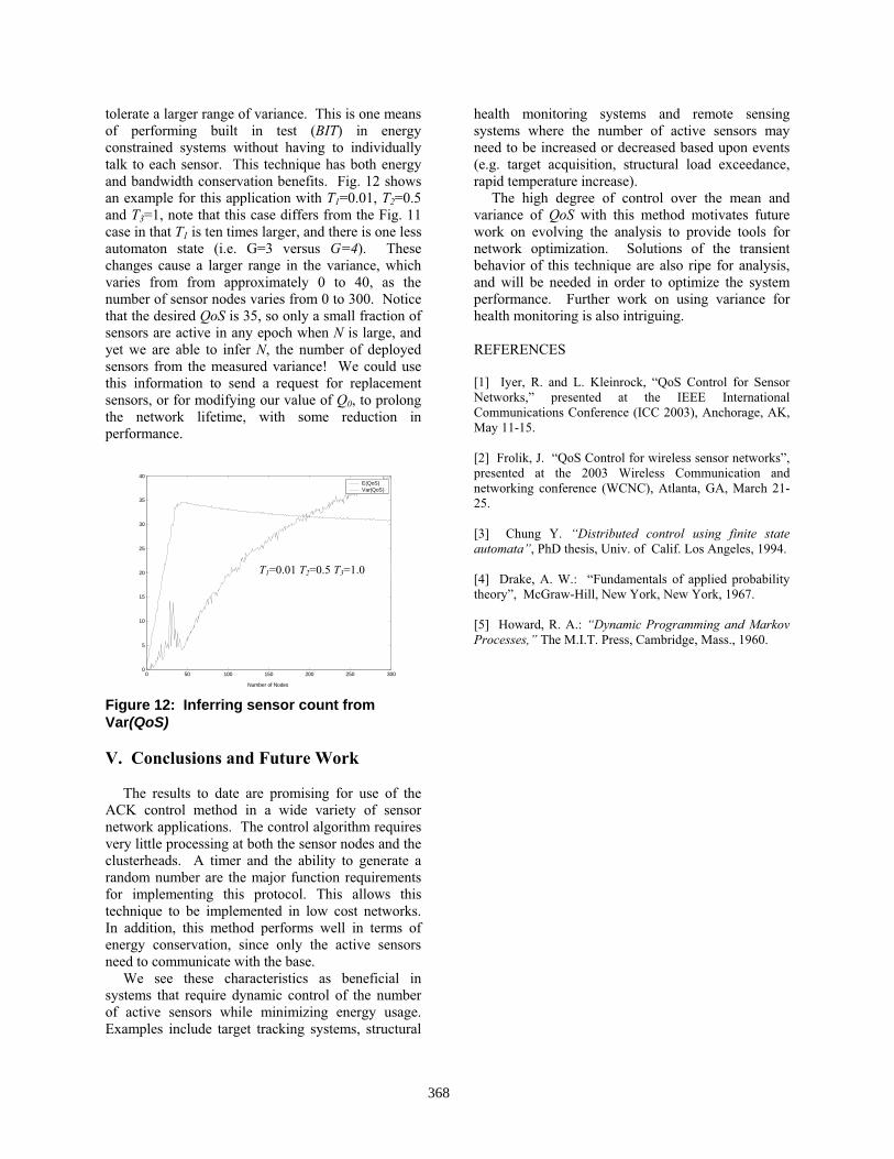
tolerate a larger range of variance. This is one means

of performing built in test (BIT) in energyconstrained systems without having to individually

talk to each sensor. This technique has both energy

and bandwidth conservation benefits. Fig. 12 showsan example for this application with T1=0.01, T2=0.5

and T3=1, note that this case differs from the Fig. 11

case in that T1 is ten times larger, and there is one lessautomaton state (i.e. G=3 versus G=4). These

changes cause a larger range in the variance, which

varies from from approximately 0 to 40, as the number of sensor nodes varies from 0 to 300. Notice

that the desired QoS is 35, so only a small fraction of sensors are active in any epoch when N is large, and

yet we are able to infer N, the number of deployed

sensors from the measured variance! We could usethis information to send a request for replacement

sensors, or for modifying our value of Q0, to prolong

the network lifetime, with some reduction inperformance.

0 50 100 150 200 250 3000

5

10

15

20

25

30

35

40

Number of Nodes

E(QoS)Var(QoS)

T1=0.01 T2=0.5 T3=1.0

Figure 12: Inferring sensor count fromVar(QoS)

V. Conclusions and Future Work

The results to date are promising for use of theACK control method in a wide variety of sensor

network applications. The control algorithm requires

very little processing at both the sensor nodes and theclusterheads. A timer and the ability to generate a

random number are the major function requirementsfor implementing this protocol. This allows this

technique to be implemented in low cost networks.

In addition, this method performs well in terms of energy conservation, since only the active sensors

need to communicate with the base.

We see these characteristics as beneficial in systems that require dynamic control of the number

of active sensors while minimizing energy usage.

Examples include target tracking systems, structural

health monitoring systems and remote sensing

systems where the number of active sensors mayneed to be increased or decreased based upon events

(e.g. target acquisition, structural load exceedance,

rapid temperature increase).The high degree of control over the mean and

variance of QoS with this method motivates future

work on evolving the analysis to provide tools fornetwork optimization. Solutions of the transient

behavior of this technique are also ripe for analysis,

and will be needed in order to optimize the systemperformance. Further work on using variance for

health monitoring is also intriguing.

REFERENCES

[1] Iyer, R. and L. Kleinrock, “QoS Control for Sensor

Networks,” presented at the IEEE International

Communications Conference (ICC 2003), Anchorage, AK,

May 11-15.

[2] Frolik, J. “QoS Control for wireless sensor networks”,

presented at the 2003 Wireless Communication and

networking conference (WCNC), Atlanta, GA, March 21-

25.

[3] Chung Y. “Distributed control using finite state

automata”, PhD thesis, Univ. of Calif. Los Angeles, 1994.

[4] Drake, A. W.: “Fundamentals of applied probability

theory”, McGraw-Hill, New York, New York, 1967.

[5] Howard, R. A.: “Dynamic Programming and Markov

Processes,” The M.I.T. Press, Cambridge, Mass., 1960.

368