Embed Size (px)
Citation preview

Plan for the course
• Tuesday p.m¤ Lecture 1
¤ Lecture 2
• Wednesday a.m.¤ Lecture 3
• Wednesday p.m.¤ Practical Session

QM/MM Modelling
Lecture 1Concepts and Theory

Overview
• Rationale
• Notation¤ inner, outer boundary, link etc
• Historical overview
• Energy expression¤ Additive vs Subtractive
• QM/MM Coupling ¤ Mechanical, electrostatic, polarised
• Link Atom treatments
• Choice of QM and MM models
• Conformational complexity¤ Geometry optimisation algorithms

The QM/MM Modelling Approach
• Couple quantum mechanics and molecular mechanics approaches
• QM treatment of the active site¤ reacting centre¤ excited state processes (e.g. spectroscopy)¤ problem structures (e.g. complex transition
metal centre)
• Classical MM treatment of environment¤ enzyme structure¤ zeolite framework¤ explicit solvent molecules¤ bulky organometallic ligands

Terminology
• Usually we can view QM/MM calculations as a combination of
¤ a QM calculation on a small region of the system
¤ A surrounding environment modelled by a MM calculation
• Optionally, some treatment, e.g. dielectric response of the region outside the outer region is included.
Inner Region Outer Region
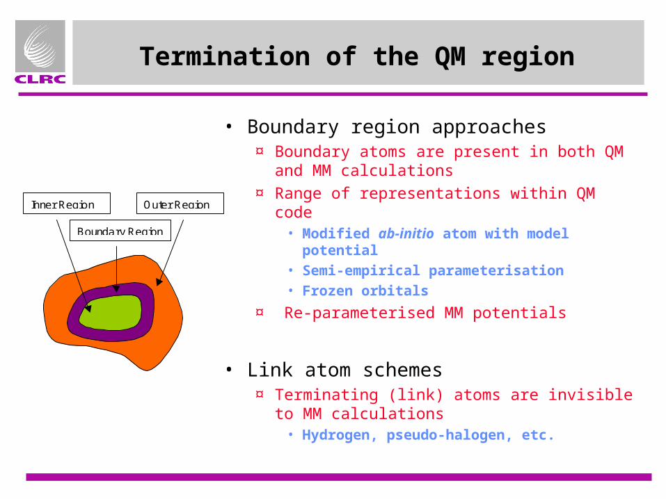
Termination of the QM region
• Boundary region approaches¤ Boundary atoms are present in both QM and
MM calculations
¤ Range of representations within QM code• Modified ab-initio atom with model potential• Semi-empirical parameterisation• Frozen orbitals
¤ Re-parameterised MM potentials
• Link atom schemes¤ Terminating (link) atoms are invisible to MM
calculations• Hydrogen, pseudo-halogen, etc.
Inner Region
Boundary Region
Outer Region
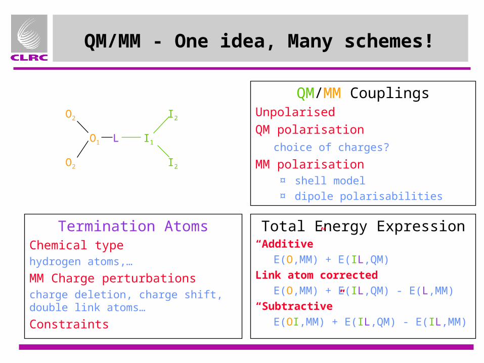
QM/MM - One idea, Many schemes!
Termination AtomsChemical typehydrogen atoms,…
MM Charge perturbationscharge deletion, charge shift, double link atoms…
Constraints
QM/MM CouplingsUnpolarised
QM polarisation
choice of charges?
MM polarisation¤ shell model¤ dipole polarisabilities
Total Energy Expression“Additive”
E(O,MM) + E(IL,QM)
Link atom corrected
E(O,MM) + E(IL,QM) - E(L,MM)
“Subtractive”
E(OI,MM) + E(IL,QM) - E(IL,MM)
O1
O2
I1
I2
L
O2 I2
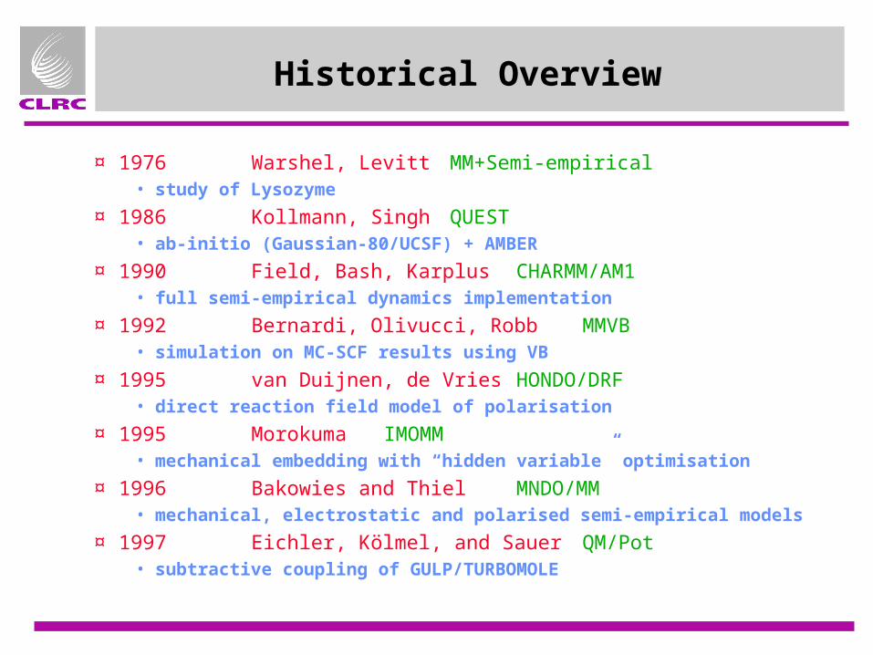
Historical Overview
¤ 1976 Warshel, Levitt MM+Semi-empirical• study of Lysozyme
¤ 1986 Kollmann, Singh QUEST • ab-initio (Gaussian-80/UCSF) + AMBER
¤ 1990 Field, Bash, Karplus CHARMM/AM1• full semi-empirical dynamics implementation
¤ 1992 Bernardi, Olivucci, Robb MMVB• simulation on MC-SCF results using VB
¤ 1995 van Duijnen, de Vries HONDO/DRF• direct reaction field model of polarisation
¤ 1995 Morokuma IMOMM• mechanical embedding with “hidden variable” optimisation
¤ 1996 Bakowies and Thiel MNDO/MM• mechanical, electrostatic and polarised semi-empirical models
¤ 1997 Eichler, Kölmel, and Sauer QM/Pot• subtractive coupling of GULP/TURBOMOLE

Additive Energy Expressions
• Energy Expressions¤ Without link atom correction
E(O,MM) + E(I,QM) + E(IO,QM/MM)¤ Link atom correction
E(O,MM) + E(IL,QM) + E(IO,QM/MM)
- E(L,MM) ¤ Boundary methods
E(OB,MM) + E(IB,QM) + E(IBO,QM/MM)
• Highly variable in implementation¤ QM/MM couplings,¤ QM termination etc
• Advantages¤ No requirement for forcefield for
reacting centre¤ Can naturally build in electrostatic
polarisation of QM region - effects of environment of excitations etc
• Disadvantages¤ Electrostatic coupling of the two
regions, E(IO,QM/MM) is problematic with link atoms
¤ Need for boundary atom parameterisation
• Applications¤ Solvation¤ Enzymes¤ Zeolites

Subtractive QM/MM Coupling
• Energy ExpressionE(OI,MM) + E(IL,QM) - E(IL,MM) ¤ includes link atom correction¤ can treat polarisation of both the
MM and QM regions at the force-field level
• Termination¤ Any (provided a force field model
for IL is available)
• Advantages¤ Potentially highly accurate and free
from artefacts¤ Can also be used for QM/QM
schemes (e.g. IMOMO, Morokuma et al)
• Disadvantages¤ Need for accurate forcefields
(mismatch of QM and MM models can generate catastrophes on potential energy surface)
¤ No electrostatic influence on QM wavefunction included
• Applications¤ Zeolites (Sauer et al) ¤ Organometallics (Morokuma et al)

Choice of QM Model
Applicability¤ Most QM methods are suitable
• semi-empirical• Empirical valence bond (Warshel, MOLARIS)• MM-VB (Robb, fitted to CASSCF)• ab-initio• DFT
– Gaussian basis – Plane wave (CP) - Zeigler, Parrinello, Rothlisburger
Attributes¤ For electrostatic embedding need to insert extra nuclei in Hamiltonian
• Cost implications, eg derivatives, Hessians
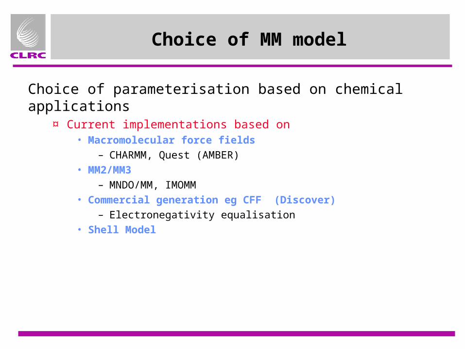
Choice of MM model
Choice of parameterisation based on chemical applications¤ Current implementations based on
• Macromolecular force fields– CHARMM, Quest (AMBER)
• MM2/MM3 – MNDO/MM, IMOMM
• Commercial generation eg CFF (Discover)– Electronegativity equalisation
• Shell Model

Valence Force Fields (i)
• Used for covalently bound molecules and networks
• Terms associated with bonded groups¤ bonds
• e.g. harmonic, quartic
¤ angles• e.g. harmonic, quartic
¤ dihedral (torsion) angles• sin,cos (rotational barriers)• harmonic (e..g planarity constraints)
¤ sometimes other cross-terms• bond-bond coupling• bond-angle coupling

Valence forcefields (ii)
• Non-bonded terms¤ Summed over all non-covalently-bound pairs
• always exclude bonded pairs• exclude 1,3 interactions for angles• sometimes scale 1,4 interactions for dihedrals
¤ van der Waals• Buckingham, Lennard-Jones
¤ electrostatics• simple coulomb (qiqj/r)
– Need to decide the atomic charges … • distance-dependent dielectric
– Approximate correction for solvation
• Examples¤ MM2, AMBER, CHARMM, UFF, CFF, CVFF

Shell Model Force fields
• Typically used for ionic solids
• Leading terms are non-bonded¤ Electrostatics
• often based on formal charges• polarisability of ions included by splitting
total ion charge in – Core (often +ve) and Shell (-ve),
modelling the valence electrons– Shell can shift in response to electrostatic
forces, restoring forces from harmonic “spring”
¤ van der Waals• sometimes compute using shell position
• Can also incorporate 3-body terms • some bond angles are preferred over
others, introducing some covalent character
Shell position
Core position

Choice of MM Model
¤ Practical considerations• for link atoms schemes must be able to remove selected forcefield terms
from topology• need vdW parameters for interaction with QM (always)• QM charges and/or forcefield terms (sometimes)• numerical noise (e.g. cutoffs) important for transition states etc.
¤ Future prospects• DMA, polarisabilities

QM/MM Non-bonded Interactions
¤ Short-range forces (van der Waals)• Typically will follow MM conventions (pair potentials etc), sometimes
reparameterisation is performed to reflect replacement of point charges interactions with QM/MM electrostatic terms.
¤ Electrostatic interactions:• Mechanical Embedding
in vacuo QM calculation coupled classically to MM via point charges at QM nuclear sites
• Electrostatic Embedding
MM atoms appear as centres generating electrostatic contribution to QM Hamiltonian
• Polarised Embedding
MM polarisability is coupled to QM charge density
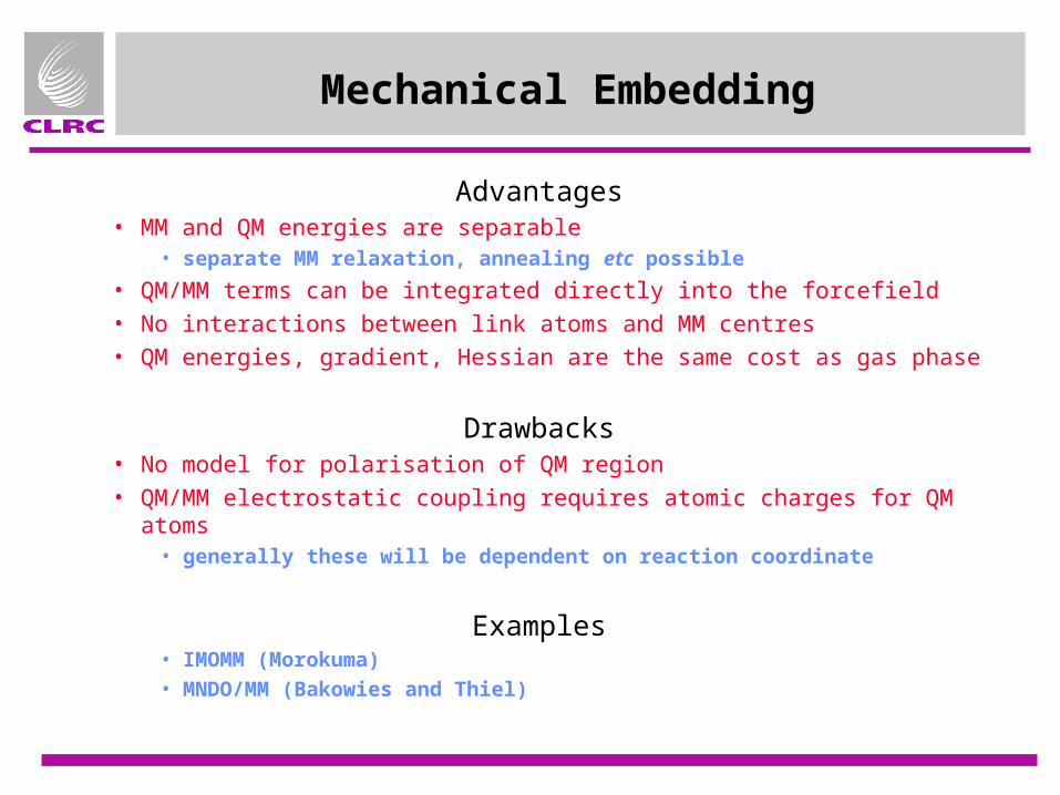
Mechanical Embedding
Advantages• MM and QM energies are separable
• separate MM relaxation, annealing etc possible
• QM/MM terms can be integrated directly into the forcefield• No interactions between link atoms and MM centres• QM energies, gradient, Hessian are the same cost as gas phase
Drawbacks• No model for polarisation of QM region• QM/MM electrostatic coupling requires atomic charges for QM atoms
• generally these will be dependent on reaction coordinate
Examples• IMOMM (Morokuma)• MNDO/MM (Bakowies and Thiel)

Electrostatic Embedding
(i) Assign MM Charges for pure MM system• Derived from empirical schemes (e.g. as part of forcefield)• Fitted to electrostatic potentials• Formal charges (e.g. shell model potentials)• Electronegativity equalisation (e.g. QEq)
(ii) Delete MM charges on atoms in inner region• Attempt to ensure that MM “defect” + terminated QM region has
– correct total charge– approximately correct dipole moment
(iii) Insert charges on MM centres into QM Hamiltonian• Explicit point charges• Smeared point charges• Semi-empirical core interaction terms• Make adjustments to closest charges (deletion, shift etc)

Creation of neutral embedding site (i) Neutral charge groups
• Deletion according to force-field neutral charge-group definitions
C
NC
C
O
H R
N
H
C
O
R

Creation of neutral embedding site (i) Neutral charge groups
• Total charge conserved, poor dipole moments
C
NC
C
O
H R
N
H
C
O
R
H H

Creation of neutral embedding site (ii) Polar forcefields
bond dipole models, e.g. for zeolites (Si +0.5x, O -0.5x)
O-x O-x
O-x
O-x
Si+2x

Creation of neutral embedding site (ii) Polar forcefields
O-0.5x O-0.5x
O-0.5x
O-0.5x
Si
H
H
HH

Creation of neutral embedding site (iii) Double link atoms
• Suggestion from Brooks (NIH) for general deletion (not on a force-field neutral charge-group boundary)
C
NC
C
O
H R
N
H
C
O
R

Creation of neutral embedding site (iii) Double link atoms
• All fragments are common chemical entities, automatic charge assignment is possible.
C
N
CC
O
HR
N
H
C
O
R
H H
H H

Boundary adjustments
¤ Some of the classical centres will lie close to link atom (L)
¤ Artefacts can result if charge at the M1
centre is included in Hamiltonian, many adjustment schemes have been suggested
• Adjustments to polarising field can be made independently from specification of MM…MM interactions
• Similar adjustments may are needed if M1
is classified as a boundary atom, depending on M1 treatment.
M2
M1 Q1
Q2
Q2M2
M3 Q3
L

Boundary Adjustments (i)Selective deletion of 1e integrals
¤ L1: Delete integrals for which basis functions i or j are sited on the link atom L• found to be effective for semi-empirical wavefunctions• difference in potential acting on nearby basis functions causes unphysical polarisation for
ab-initio QM models
¤ L3: Delete integrals for which basis functions i and j are cited on the link atom and qA is the neighbouring MM atom (M1)
• less consistent results observed in practice †
† Classification from Antes and Thiel, in Combined Quantum Mechanical and Molecular Mechanical Methods, J. Gao and M. Thompson, eds. ACS Symp. Ser., Washington DC, 1998.
lr
qlV j
lA
Ai
Aij

Boundary Adjustments (ii)Deletion of first neutral charge group
¤ L2 - Exclude charges on all atoms in the neutral group containing M1
• Maintains correct MM charge– leading error is the missing dipole moment of the first charge group
• Generally reliable – free from artefacts arising from close contacts
• Limitations– only applicable in neutral group case (e.g. AMBER, CHARMM)– neutral groups are highly forcefield dependent– problematic if a charge group needs to be split
• Application – biomolecular systems

Creation of neutral embedding site Double Link Atoms
• Conventional QM/MM schemes¤ Break into H3C and CH3
• Neutral fragments (in this simple case)
• Non-zero individual dipoles
¤ Replace QM CH3 with some form of terminated group (L-CH3)
• Finite total dipole moment
• Often further adjustment to MM charges is required (may create additional charge and dipole errors).
• Double link atom• Dipole generally well approximated by
superposition of bonds
C C
H
H
H H
H
H
C C
H
H
H H
H
H
H
MM QM
C C
H
H
H H
H
H
HH

Boundary adjustments (iv) Gaussian Blur
¤ Delocalise point charge using Gaussian shape function• Large Gaussian width : electrostatic coupling disappears• Narrow Gaussian width : recover point charge behaviour• Intermediate values
– short range interactions are attenuated– long range electrostatics are preserved
¤ Importance of balance - apply to entire MM system or to first neutral group
¤ Particularly valuable for double-link atom scheme where MM link atom charge lies within QM molecular envelope
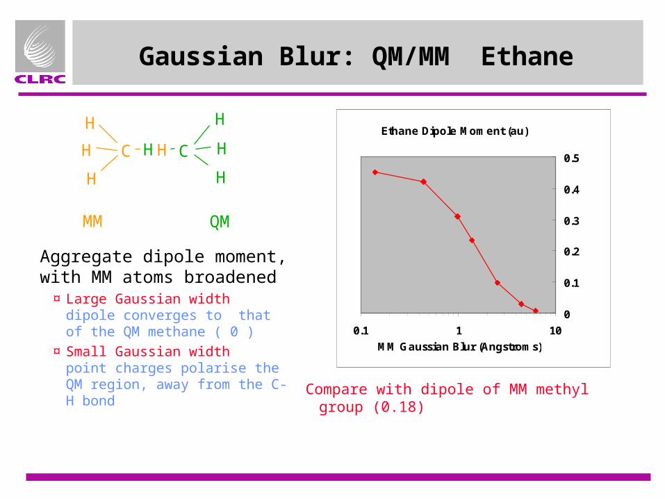
Gaussian Blur: QM/MM Ethane
Aggregate dipole moment, with MM atoms broadened
¤ Large Gaussian width dipole converges to that of the QM methane ( 0 )
¤ Small Gaussian width point charges polarise the QM region, away from the C-H bond
MM QM
C C
H
H
H H
H
H
HH
Compare with dipole of MM methyl group (0.18)
Ethane Dipole Moment (au)
0
0.1
0.2
0.3
0.4
0.5
0.1 1 10
MM Gaussian Blur (Angstroms)
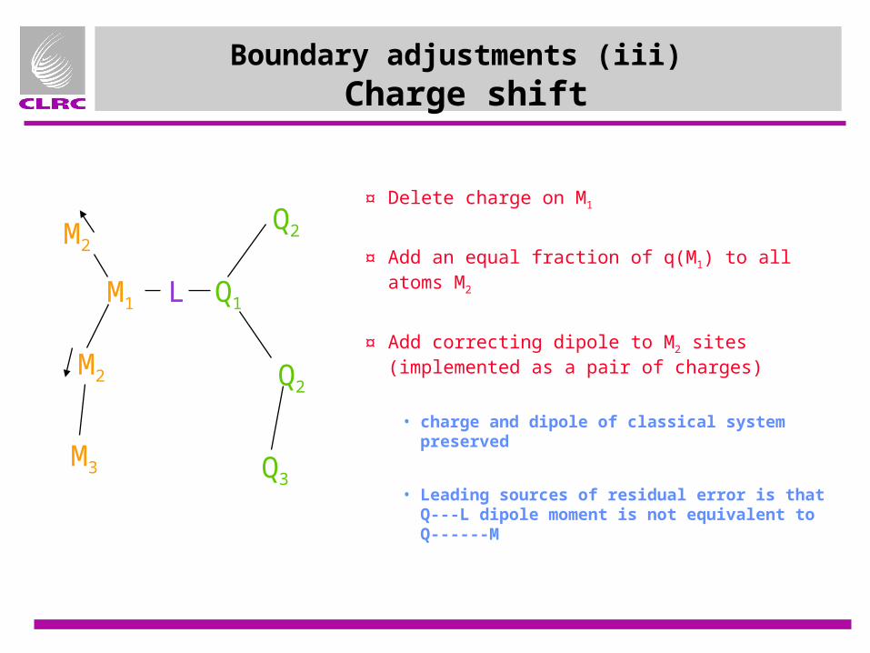
Boundary adjustments (iii) Charge shift
¤ Delete charge on M1
¤ Add an equal fraction of q(M1) to all atoms M2
¤ Add correcting dipole to M2 sites (implemented as a pair of charges)
• charge and dipole of classical system preserved
• Leading sources of residual error is that Q---L dipole moment is not equivalent to Q------M
M2
M1 Q1
Q2
Q2M2
M3 Q3
L

QM/MM coupling - Proton Affinity Tests
• Simplified alcohol test set based on [1]¤ AMBER charge model
¤ QM region is small (HOCH3 in all cases)
¤ Include systems with 1, 2 and 3 link atoms, Ethanol, i-Propanol, t-Butanol
¤ Fixed geometries (from 3-21G QM optimisations)
¤ Compare• Pure QM• L2 (delete first charge group)• Shift (move charge from first atom to
neighbours, add dipole.• Double link atom + Gaussian Blur
H
C CH3O
CH3
CH3
H
C CH3O
CH3
H
H
CO
CH3
H
H
[1] I. Antes and W. Thiel, in “Hybrid Quantum Mechanical and Molecular Mechanical
Methods” J. Gao (ed.) ACS Symp.Ser. 712, ACS, Washington, DC, 1998.
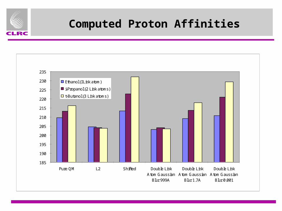
Computed Proton Affinities
185
190
195
200
205
210
215
220
225
230
235
Pure QM L2 Shifted Double LinkAtom Gaussian
Blur 999A
Double LinkAtom Gaussian
Blur 1.7A
Double LinkAtom Gaussian
Blur 0.001
Ethanol (I Link atom)
i-Propanol (2 Link atoms)
t-Butanol (3 Link atoms)

Electrostatic EmbeddingSummary
Advantages• Capable of treating changes in charge density of QM
• important for solvation energies etc
• No need for a charge model of QM region• can readily model reactions that involve charge separation
Drawbacks• Charges must provide a reliable model of electrostatics
• reparameterisation may be needed for some forcefields
• Danger of spurious interactions between link atoms and charges
• QM evaluation needed to obtain accurate MM forces
• QM energy, gradient, Hessian are more costly than gas phase QM
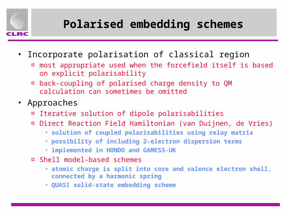
Polarised embedding schemes
• Incorporate polarisation of classical region¤ most appropriate used when the forcefield itself is based on explicit
polarisability
¤ back-coupling of polarised charge density to QM calculation can sometimes be omitted
• Approaches¤ Iterative solution of dipole polarisabilities
¤ Direct Reaction Field Hamiltonian (van Duijnen, de Vries)• solution of coupled polarisabilities using relay matrix• possibility of including 2-electron dispersion terms• implemented in HONDO and GAMESS-UK
¤ Shell model-based schemes• atomic charge is split into core and valence electron shell, connected by
a harmonic spring• QUASI solid-state embedding scheme

QM
Solid-state Embedding Scheme
• Classical cluster termination¤ Base model on finite MM cluster¤ QM region sees fitted correction
charges at outer boundary
• QM region termination¤ Ionic pseudopotentials (e.g. Zn2+,
O2-) associated with atoms in the boundary region
• Forcefield¤ Shell model polarisation¤ Classical estimate of long-range
dielectric effects (Mott/Littleton)
• Energy Expression¤ Uncorrected
• Advantages¤ suitable for ionic materials
• Disadvantages¤ require specialised pseudopotentials
• Applications¤ metal oxide surfaces
MM

Implementation of solid-state embedding
¤ Under development by Royal Institution and Daresbury
¤ Based on shell model code GULP, from Julian Gale (Imperial College)
¤ Both shell and core positions appear as point charges in QM code (GAMESS-UK)
¤ Self-consistent coupling of shell relaxation
• Import electrostatic forces on shells from GAMESS-UK
• relax shell positions
GULP shell relaxation
GAMESS-UK SCF & shell forces
GAMESS-UK atomic forces
GULP forces

Polarised Embedding SchemesSummary
• Advantages¤ more accurate treatment of solvation effects
¤ allows coupling to systems where the best forcefields are based on polarisation (e.g. shell model potentials for metal oxide systems)
• Drawbacks¤ Additional cost
• solution of coupled polarisabilities• some schemes will require additional SCF iterations
¤ requirement for polarised force-field
¤ danger of electrostatic instabilities close to boundaries• difficult to apply reliably when using link atoms

QM Termination Schemes
• Link atom schemes¤ Hydrogen atoms¤ Adjusted electronegativity
• Hamiltonian shift operator• pseudohalogen (Hyperchem)
¤ Methyl groups (Cummins, Gready)
• Boundary schemes¤ Frozen Orbitals
• Local SCF scheme (Rivail)• Generalised hybrid orbital (Gao)• ab-initio implementation (Friesner)
¤ Pseudopotentials• Gaussian basis (Yang), Plane-wave (Rothlisberger)
¤ Adjusted connection atoms (Thiel)• semi-empirical mimic for attached methyl group

Adjusted Connection Atoms
• Semi-empirical parameterisation of boundary atom¤ Implemented in the MNDO package (Thiel el a)
¤ No link atoms needed, boundary atom sited at MM centre
¤ Typically boundary atom is C, parameterised to mimic CH3
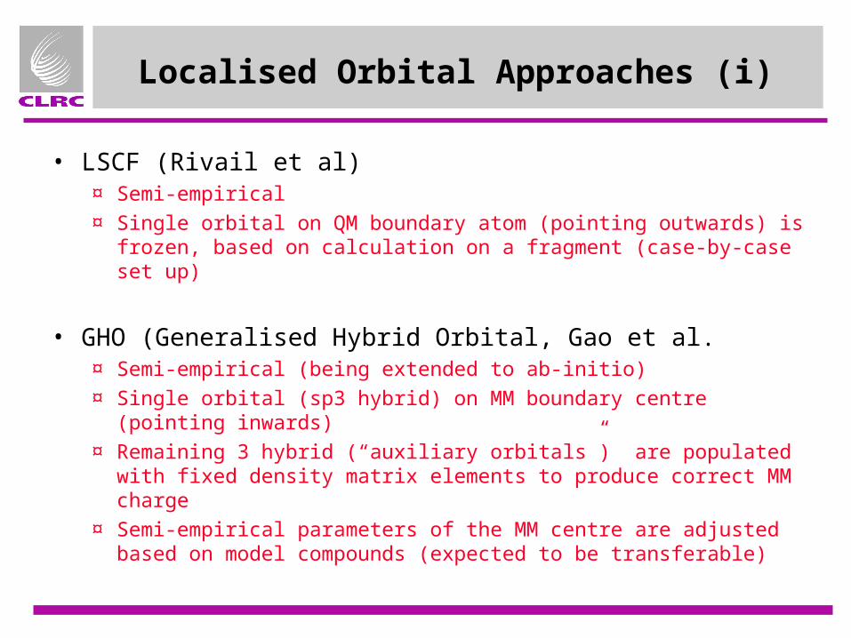
Localised Orbital Approaches (i)
• LSCF (Rivail et al)¤ Semi-empirical
¤ Single orbital on QM boundary atom (pointing outwards) is frozen, based on calculation on a fragment (case-by-case set up)
• GHO (Generalised Hybrid Orbital, Gao et al.¤ Semi-empirical (being extended to ab-initio)
¤ Single orbital (sp3 hybrid) on MM boundary centre (pointing inwards)
¤ Remaining 3 hybrid (“auxiliary orbitals”) are populated with fixed density matrix elements to produce correct MM charge
¤ Semi-empirical parameters of the MM centre are adjusted based on model compounds (expected to be transferable)

Localised orbital Approaches (ii)
• QSite implementation (Friesner et al)
¤ Ab-initio implementation, in Jaguar package
¤ Based on calculations on model fragments, using a particular basis set
¤ Local orbitals include contribution from connected atoms (not just the QM and MM centres
¤ Adjustment of MM parameters performed on a case-by-case basis, currently being used for protein system

• Initial placement¤ Usually on terminated bond
• Unconstrained¤ Additional degrees of freedom present in geometry optimisation and MD
• e.g. CHARMM, QUEST
• Constrained¤ Need to take into account forces on link atoms,
• shared internal coordinate definitions (IMOMM) • chain-rule differentiation (QM/Pot, ChemShell)
Positioning of link atoms
111 M
L
LMM x
x
x
E
x
E
x
E
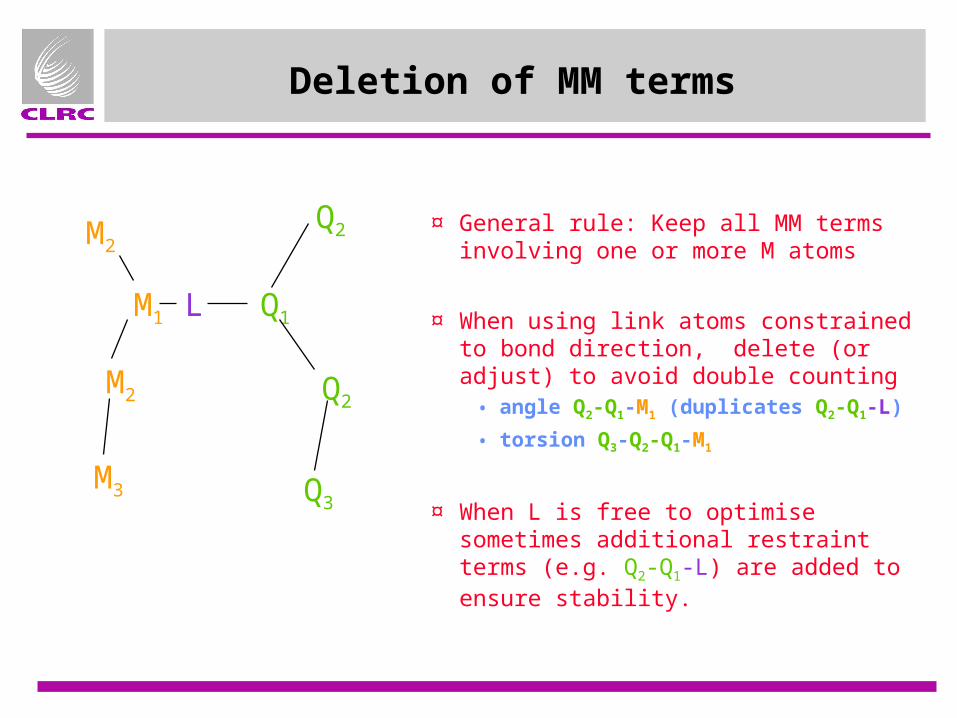
Deletion of MM terms
¤ General rule: Keep all MM terms involving one or more M atoms
¤ When using link atoms constrained to bond direction, delete (or adjust) to avoid double counting
• angle Q2-Q1-M1 (duplicates Q2-Q1-L)
• torsion Q3-Q2-Q1-M1
¤ When L is free to optimise sometimes additional restraint terms (e.g. Q2-Q1-L) are added to ensure stability.
M2
M1 Q1
Q2
Q2M2
M3 Q3
L

Conformational Complexity
The Problem!¤ QM/MM schemes combine
• the cost of QM• the computational complexity of large MM systems
¤ Special treatments are needed for flexible molecules• For mechanical embedding, hidden variables can reduce number of
coordinates by exploring QM PES in presence of adiabatically relaxed MM environment (eg IMOMM)
• For electrostatic embedding, a charge fit to the QM charge density can be used to accelerate MM relaxation around a frozen QM core
– A.J. Turner et al, PCCP 1, p1323, 1999– Zhang et al, J. Chem. Phys., 112, p3483, 2000
¤ Molecular dynamics and free energy techniques will be increasingly important
• computationally demanding for ab-initio QM, requirement for HPC implementations

QM/MM Geometry Optimisation
Small Molecules• Internal coordinates (delocalised,
redundant etc)• Full Hessian• O(N3) cost per step
¤ BFGS, P-RFO
Macromolecules• Cartesian coordinates• Partial Hessian (e.g. diagonal)• O(N) cost per step
¤ Conjugate gradient¤ L-BFGS
Coupled QM/MM schemes¤ Combine cartesian and internal coordinates
¤ Reduce cost of manipulating B, G matrices¤ Define subspace (core region) and relax environment at each step
¤ reduce size of Hessian ¤ exploit greater stability of minimisation vs. TS algorithms¤ Use approximate scheme for environmental relaxation
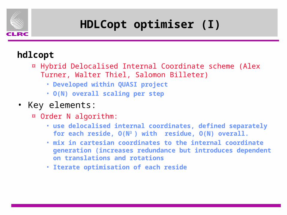
HDLCopt optimiser (I)
hdlcopt ¤ Hybrid Delocalised Internal Coordinate scheme (Alex Turner, Walter
Thiel, Salomon Billeter) • Developed within QUASI project• O(N) overall scaling per step
• Key elements:¤ Order N algorithm:
• use delocalised internal coordinates, defined separately for each reside, O(N3 ) with residue, O(N) overall.
• mix in cartesian coordinates to the internal coordinate generation (increases redundance but introduces dependent on translations and rotations
• Iterate optimisation of each reside

HDLC Optimiser (ii)
¤ Residue specification, often taken from a pdb file (pdb_to_res) allows separate delocalised coordinates to be generated for each residue
¤ Can perform P-RFO TS search in the first residue with relaxation of the others
• increased stability for TS searching• Much smaller Hessians
¤ Further information on algorithm• S.R. Billeter, A.J. Turner and W. Thiel, PCCP 2000, 2, p 2177
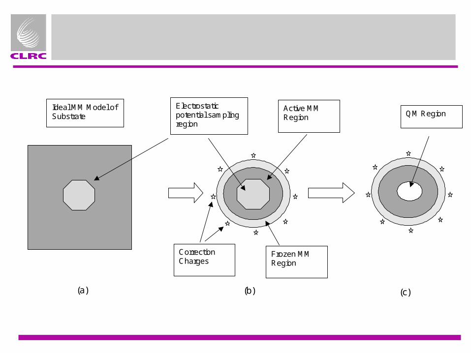
Active MMRegion
Ideal MM Model ofSubstrate
Frozen MMRegion
CorrectionCharges
QM RegionElectrostaticpotential samplingregion
(a) (b) (c)
QM/MM Modelling
Lecture 2QM/MM Implementations
Outline
• Implementation Issues¤ what factors affect the design
• Three QM/MM software approaches¤ QM added as an extension to forcefield¤ MM environment added to a small-molecule treatment¤ Modular scheme with a range of QM and MM methods
• ChemShell¤ Concepts and sample modules¤ Approaches to periodic systems
• High Performance Computing¤ Approach within QUASI¤ Parallel computing techniques within GAMESS-UK, DL_POLY etc
• Tutorial Session¤ Simple Tcl & ChemShell scripts, using the PyMOL GUI
Implementation Issues
• Most implementations are based on existing QM and MM packages
• Implementers face a basic conflict between ¤ modularity
• keeping programs separate• minimal modifications to allow easy upgrades
¤ Performance and Functionality• supporting more complex interactions• minimising overhead, recalculation, file access etc
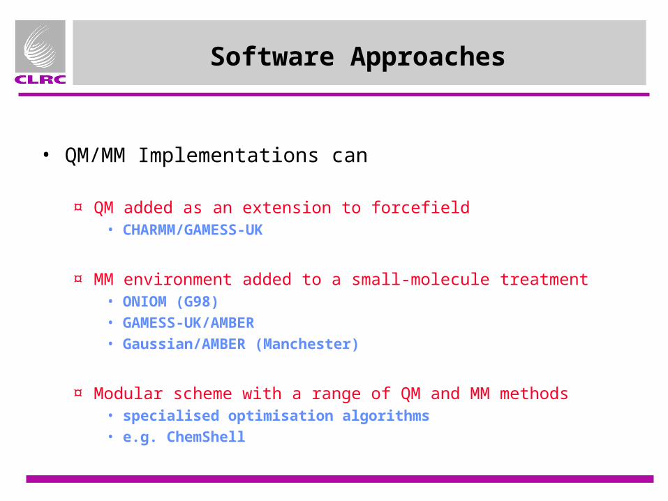
Software Approaches
• QM/MM Implementations can
¤ QM added as an extension to forcefield• CHARMM/GAMESS-UK
¤ MM environment added to a small-molecule treatment• ONIOM (G98)• GAMESS-UK/AMBER• Gaussian/AMBER (Manchester)
¤ Modular scheme with a range of QM and MM methods • specialised optimisation algorithms• e.g. ChemShell

QM/MM Software Approach (i)
• Specialised for a classical modelling approach, by integrating QM code into MM package¤ CHARMM + GAMESS(US), MNDO (Harvard & NIH)
¤ AMBER + Gaussian (UCSF, Manchester)
¤ QM/Pot, GULP + TURBOMOLE (Berlin)
¤ CHARMM + GAMESS (UK) • Daresbury & Bernie Brooks, Eric Billings (NIH)• Similar to existing ab-initio interfaces; CHARMM side follows
coupling to GAMESS(US) (Milan Hodoscek)• Support for Gaussian delocalised point charges
• Advantages¤ Good MD capabilities, model building etc
• Disadvantages¤ Restricted to certain classes of systems by forcefield choice

QM/MM Software Approach (ii)
• Extend QM code by adding MM environment as a perturbation¤ QM code is “in control”
¤ MM environment will typically be relaxed for each QM structure (hidden coordinates)
¤ e.g. ONIOM (Gaussian), IMOMM, Gaussian/AMBER (Manchester)
• Advantages¤ Familiarity for quantum chemists
¤ Tools for small molecule manipulation (internal coordinates, transition state search etc) are available
• Disadvantages¤ Relatively poor tools for management of conformational search of
QM/MM surface, QM/MM dynamics etc

ONIOM
• Widely available, part of Gaussian98
• Subtractive energy expression
¤ E(OI,MM) + E(IL,QM) - E(IL,MM)
• Includes implementation of Forcefields¤ AMBER and UFF
• Both high and low levels can be QM (IMOMO)

QM/MM Software Approach (iii)
• Modular approach covering a range of MM and QM codes¤ e.g. ChemShell
• Advantages¤ Flexibility of applications areas
¤ Ability to choose the best QM code for the specific task
¤ Ease of update of component codes
• Disadvantages¤ Software Complexity
• range of forcefield types• wide variation in QM and MM program design• Close integration needed for performance (e.g. HPC), but weak coupling
simplifies maintenance
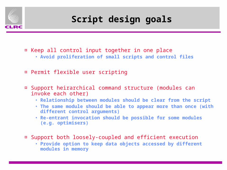
Script design goals
¤ Keep all control input together in one place• Avoid proliferation of small scripts and control files
¤ Permit flexible user scripting
¤ Support heirarchical command structure (modules can invoke each other)• Relationship between modules should be clear from the script• The same module should be able to appear more than once (with
different control arguments)• Re-entrant invocation should be possible for some modules (e.g.
optimisers)
¤ Support both loosely-coupled and efficient execution • Provide option to keep data objects accessed by different modules in
memory

ChemShell
• A Tcl interpreter for Computational Chemistry¤ Interfaces
• ab-initio (GAMESS-UK, Gaussian, CADPAC, TURBOMOLE, MOLPRO, NWChem etc)
• semi-emprical (MOPAC, MNDO)• MM codes (DL_POLY, CHARMM, GULP)
¤ optimisation, dynamics (based on DL_POLY routines)
¤ utilities (clusters, charge fitting etc)
¤ coupled QM/MM methods• Choice of QM and MM codes• A variety of QM/MM coupling schemes
– electrostatic, polarised, connection atom, Gaussian blur .. • QUASI project developments and applications e.g. Organometallics,
Enzymes, Oxides, Zeolites
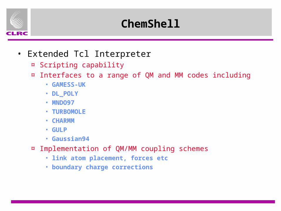
ChemShell
• Extended Tcl Interpreter¤ Scripting capability
¤ Interfaces to a range of QM and MM codes including• GAMESS-UK• DL_POLY• MNDO97• TURBOMOLE• CHARMM• GULP• Gaussian94
¤ Implementation of QM/MM coupling schemes• link atom placement, forces etc• boundary charge corrections

ChemShell Architecture - Languages
• An extended Tcl interpeter, written in..¤ Tcl
• Control scripts• Interfaces to 3rd party executables• GUI construction (Tk and itcl)• Extensions
¤ C• Tcl command implementations• Object management (fragment, matrix, field, graph)
– Tcl and C APIs– I/O
• Open GL graphics
¤ Fortran77• QM and MM codes: GAMESS-UK, GULP, MNDO97, DL_POLY

ChemShell Architecture
Core
¤ ChemShell Tcl interpreter, with code to support chemistry data:
• Optimiser and dynamics drivers
• QM/MM Coupling schemes
• Utilities
• Graphics
¤ GAMESS-UK (ab-initio, DFT)¤ MNDO (semi-empirical)¤ DL_POLY (MM)¤ GULP (Shell model, defects)
Features¤ Single executable possible¤ Parallel implementations
External Modules
¤ CHARMM¤ TURBOMOLE¤ Gaussian94¤ MOPAC¤ AMBER¤ CADPAC
Features¤ Interfaces written in Tcl¤ No changes to 3rd party codes
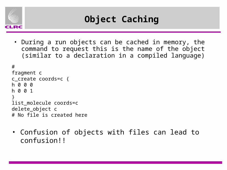
Object Caching
• During a run objects can be cached in memory, the command to request this is the name of the object (similar to a declaration in a compiled language)
#fragment cc_create coords=c {h 0 0 0h 0 0 1}list_molecule coords=cdelete_object c# No file is created here
• Confusion of objects with files can lead to confusion!!

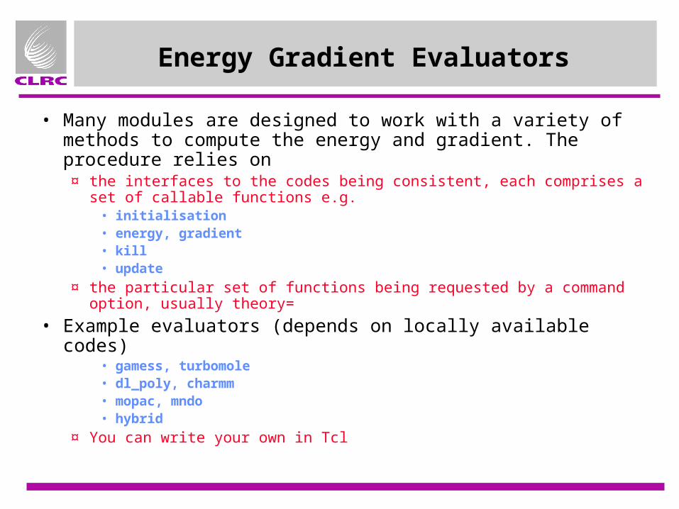
Energy Gradient Evaluators
• Many modules are designed to work with a variety of methods to compute the energy and gradient. The procedure relies on ¤ the interfaces to the codes being consistent, each comprises a set of
callable functions e.g.• initialisation• energy, gradient• kill• update
¤ the particular set of functions being requested by a command option, usually theory=
• Example evaluators (depends on locally available codes)• gamess, turbomole• dl_poly, charmm• mopac, mndo• hybrid
¤ You can write your own in Tcl

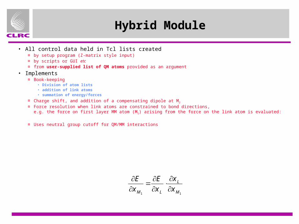
Hybrid Module
• All control data held in Tcl lists created¤ by setup program (Z-matrix style input)¤ by scripts or GUI etc¤ from user-supplied list of QM atoms provided as an argument
• Implements¤ Book-keeping
• Division of atom lists• addition of link atoms• summation of energy/forces
¤ Charge shift, and addition of a compensating dipole at M2
¤ Force resolution when link atoms are constrained to bond directions,e.g. the force on first layer MM atom (M1) arising from the force on the link atom is evaluated:
¤ Uses neutral group cutoff for QM/MM interactions
E
x
E
x
x
xM L
L
M1 1
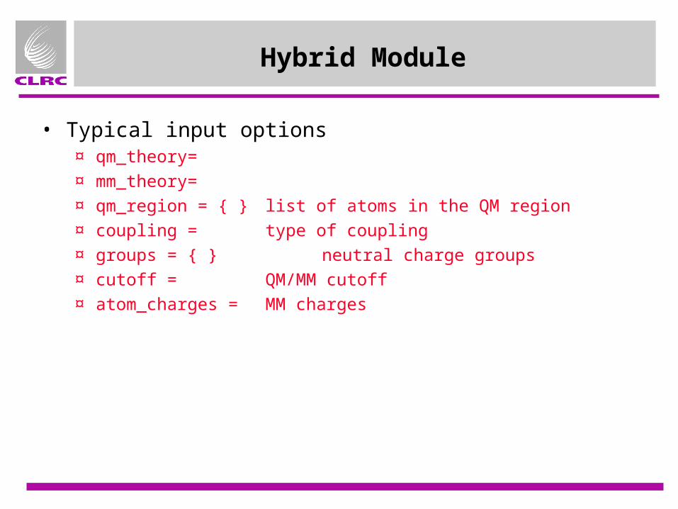
Hybrid Module
• Typical input options¤ qm_theory=
¤ mm_theory=
¤ qm_region = { } list of atoms in the QM region
¤ coupling = type of coupling
¤ groups = { } neutral charge groups
¤ cutoff = QM/MM cutoff
¤ atom_charges = MM charges

HPC Exploitation
¤ Adapt Tcl interpreter to run in parallel, master-slave architecture• one node reads input, all nodes execute commands• in-core storage of data objects
– replicated: default– distributed: specific matrix objects
¤ Use of parallel third party codes (e.g. TURBOMOLE)
¤ Direct coupling to parallel codes:• GA-based
– GAMESS-UK• MPI-based
– MNDO, GULP, DL_POLY

GAMESS-UK Parallel Implementation
¤ Replicated data scheme • store P, F, S etc on every node• minimal communications (load balancing, global sum) • up to ca. 2000 basis functions
¤ Message-passing version (MPI, TCGMSG)• SCF and DFT• Suitable for < 32 processors
¤ Global Array version: • Parallel functionality
– SCF, DFT, MP2, SCF Hessian• Parallel algorithms
– GAs for in-core storage of transformed integrals (to vvoo) and MP2 amplitudes
– parallel linear algebra (PEIGS, DIIS, MXM etc)– GA-mapped ATMOL file system
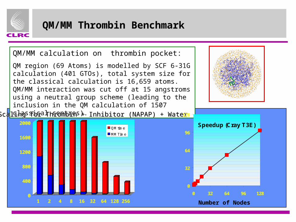
QM/MM Thrombin Benchmark
QM/MM calculation on thrombin pocket:
QM region (69 Atoms) is modelled by SCF 6-31G calculation (401 GTOs), total system size for the classical calculation is 16,659 atoms. QM/MM interaction was cut off at 15 angstroms using a neutral group scheme (leading to the inclusion in the QM calculation of 1507 classical centres).
0
400
800
1200
1600
2000
1 2 4 8 16 32 64 128 256
QM time
MM Time
Scaling for Thrombin + Inhibitor (NAPAP) + WaterScaling for Thrombin + Inhibitor (NAPAP) + Water
Speedup (Cray T3E)
0
32
64
96
128
0 32 64 96 128
Number of Nodes

QM/MM Modelling
TutorialPractical QM/MM Calculations with
the ChemShell Software
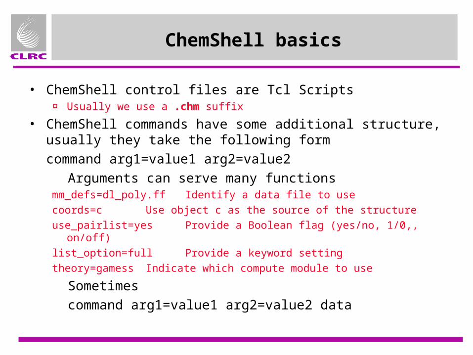
ChemShell basics
• ChemShell control files are Tcl Scripts¤ Usually we use a .chm suffix
• ChemShell commands have some additional structure, usually they take the following form
command arg1=value1 arg2=value2
Arguments can serve many functionsmm_defs=dl_poly.ff Identify a data file to use
coords=c Use object c as the source of the structure
use_pairlist=yes Provide a Boolean flag (yes/no, 1/0,, on/off)
list_option=full Provide a keyword setting
theory=gamess Indicate which compute module to use
Sometimes
command arg1=value1 arg2=value2 data

Very Simple Tcl (i)
• Variable Assignment (all variables are strings)set a 1
• Variable use[ set a ]
$a
• Command result substitution[ <Tcl command> ]
• Numerical expressions¤ set a [ expr 2 * $b ]
• Ouput to stdout¤ puts stdout “this is an output string”
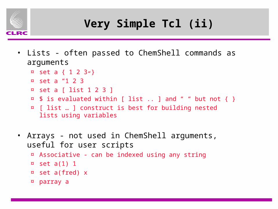
Very Simple Tcl (ii)
• Lists - often passed to ChemShell commands as arguments¤ set a { 1 2 3 }¤ set a “1 2 3”¤ set a [ list 1 2 3 ]¤ $ is evaluated within [ list .. ] and “ “ but not { }¤ [ list … ] construct is best for building nested lists using variables
• Arrays - not used in ChemShell arguments, useful for user scripts
¤ Associative - can be indexed using any string¤ set a(1) 1¤ set a(fred) x¤ parray a
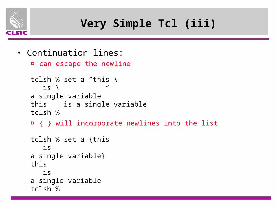
Very Simple Tcl (iii)
• Continuation lines:¤ can escape the newline
tclsh % set a “this \ is \a single variable”this is a single variabletclsh %
¤ { } will incorporate newlines into the list
tclsh % set a {this is a single variable}this is a single variabletclsh %
Very Simple Tcl (iv)
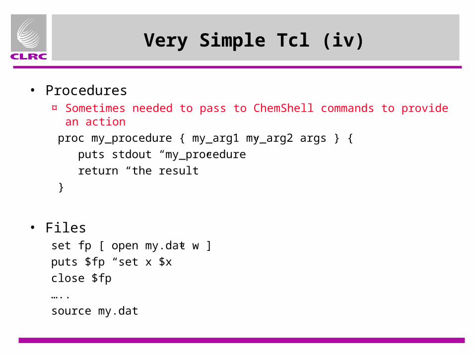
• Procedures¤ Sometimes needed to pass to ChemShell commands to provide an action
proc my_procedure { my_arg1 my_arg2 args } {
puts stdout “my_procedure”
return “the result”
}
• Filesset fp [ open my.dat w ]
puts $fp “set x $x”
close $fp
…..
source my.dat

ChemShell Object types
• ChemShell object types¤ fragment - molecular structure
• creation: c_create, load_pdb …. Universal!!
¤ zmatrix• z_create, newopt, z_surface
¤ matrix• creation: create_matrix, energy and gradient evaluators, dynamics
¤ field• creation: cluster_potential etc, graphical display, charge fits
• GUI only¤ 3dgraph

ChemShell Object Representations
• Between calculations, and sometimes between commands in a script, objects are stored as files. Usually there is no suffix, objects are distinguished internally by the block structure.
% cat cblock = fragment records = 0block = title records = 1phosphineblock = coordinates records = 34p 4.45165900000000e+00 0.00000000000000e+00 -8.17756491786826e-16 c 6.18573550000000e+00 -2.30082107458395e+00 1.93061811508830e+00 c 8.21288557680633e+00 -3.57856465464377e+00 9.30188790875432e-01 c 9.49481331797844e+00 -5.31433733714784e+00 2.37468849115612e+00 c 8.74959098234423e+00 -5.77236643959209e+00 4.81961751564967e+00……....
• Multi block objects are initiated by an empty block (e.g. fragment)• Unrecognised blocks are silently ignored

Object Caching
• During a run objects can be cached in memory, the command to request this is the name of the object (similar to a declaration in a compiled language)
#fragment cc_create coords=c {h 0 0 0h 0 0 1}list_molecule coords=cdelete_object c# No file is created here
• Confusion of objects with files can lead to confusion!!
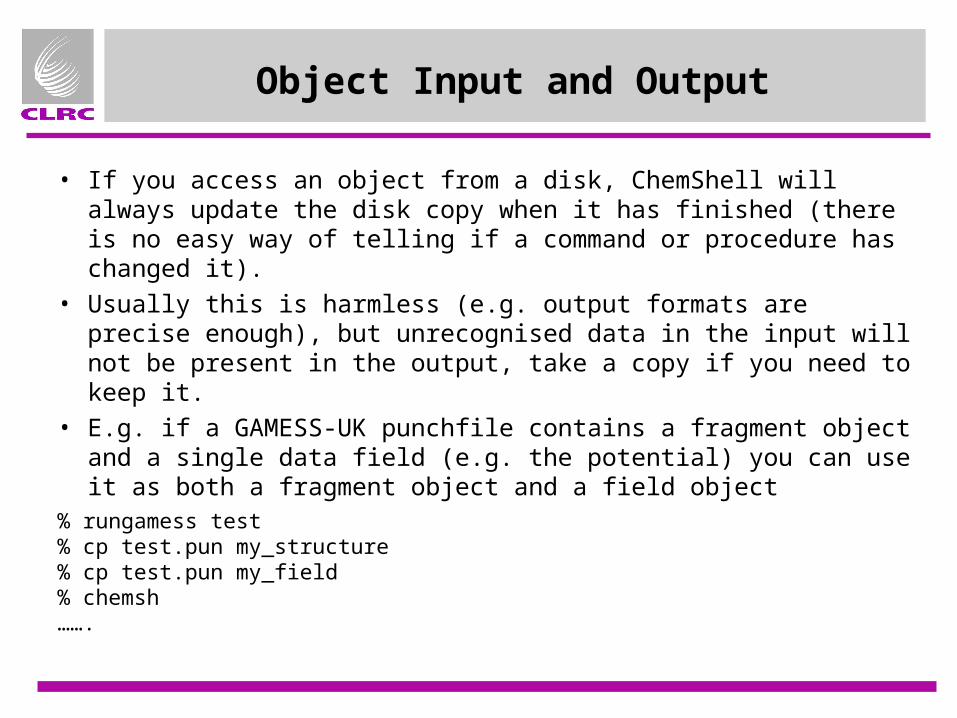
Object Input and Output
• If you access an object from a disk, ChemShell will always update the disk copy when it has finished (there is no easy way of telling if a command or procedure has changed it).
• Usually this is harmless (e.g. output formats are precise enough), but unrecognised data in the input will not be present in the output, take a copy if you need to keep it.
• E.g. if a GAMESS-UK punchfile contains a fragment object and a single data field (e.g. the potential) you can use it as both a fragment object and a field object
% rungamess test% cp test.pun my_structure% cp test.pun my_field% chemsh …….
Energy Gradient Evaluators
• Many modules are designed to work with a variety of methods to compute the energy and gradient. The procedure relies on ¤ the interfaces to the codes being consistent, each comprises a set of
callable functions e.g.• initialisation• energy, gradient• kill• update
¤ the particular set of functions being requested by a command option, usually theory=
• Example evaluators (depends on locally available codes)• gamess, turbomole• dl_poly, charmm• mopac, mndo• hybrid
¤ You can write your own in Tcl

Module options, using the :
The : syntax is used to pass control options to sub-module.
e.g. when running the optimiser, to set the options for the module computing the energy and gradient. {} can be used if there is more than one argument to pass on. Nested structures are possible using Tcl lists
newopt function=zopt : { theory=gamess : { basis=sto3g } zmatrix=z }
Command
newopt arguments
gamess arguments
zopt arguments

Loading Objects - Z-matrices
z_create zmatrix=z {zmatrix angstromcx 1 1.0n 1 cn 2 angf 1 cf 2 ang 3 phivariables cn 1.135319cf 1.287016phi 180.constantsang 90.end}
z_list zmatrix=z
set p [ z_prepare_input zmatrix=z ]puts stdout $p
• z_create provides input processor for the z-matrix object
• z_list can be used to display the object in a readable form
• z_prepare_input provides the reverse transformation if you need something to edit
• z_to_c provides the cartesian representation
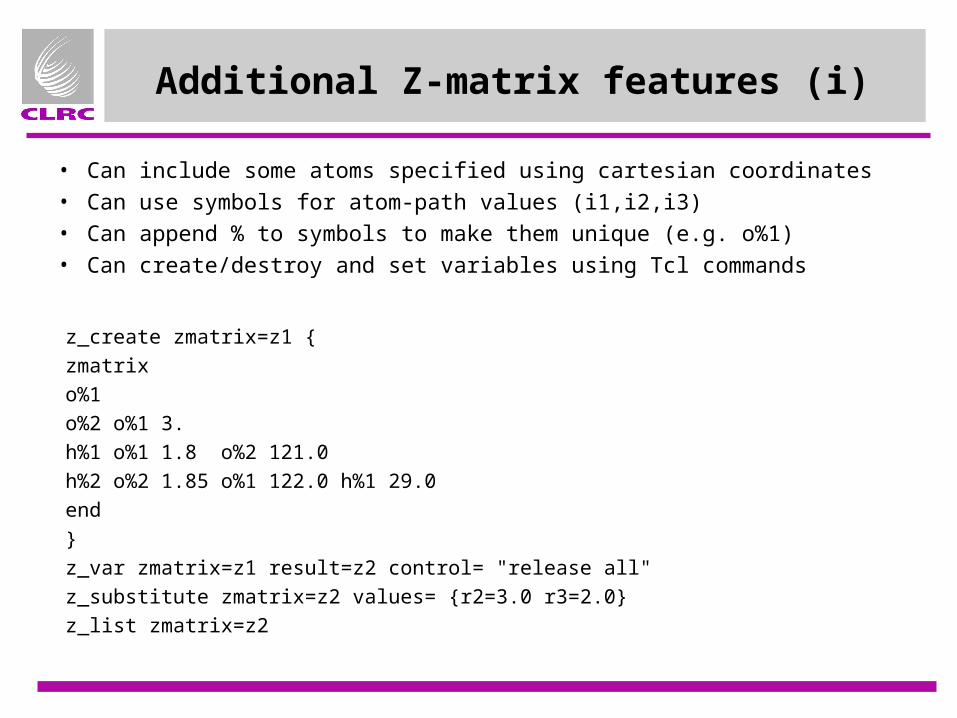
Additional Z-matrix features (i)
• Can include some atoms specified using cartesian coordinates• Can use symbols for atom-path values (i1,i2,i3)• Can append % to symbols to make them unique (e.g. o%1)• Can create/destroy and set variables using Tcl commands
z_create zmatrix=z1 {zmatrixo%1o%2 o%1 3.h%1 o%1 1.8 o%2 121.0h%2 o%2 1.85 o%1 122.0 h%1 29.0end}z_var zmatrix=z1 result=z2 control= "release all"z_substitute zmatrix=z2 values= {r2=3.0 r3=2.0}z_list zmatrix=z2
Additional Z-matrix features (ii)
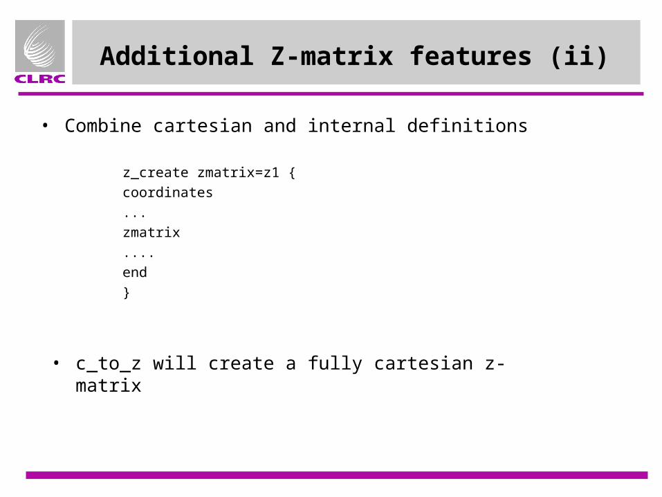
• Combine cartesian and internal definitions
z_create zmatrix=z1 {coordinates... zmatrix....end}
• c_to_z will create a fully cartesian z-matrix
Loading Data Object - Coordinates
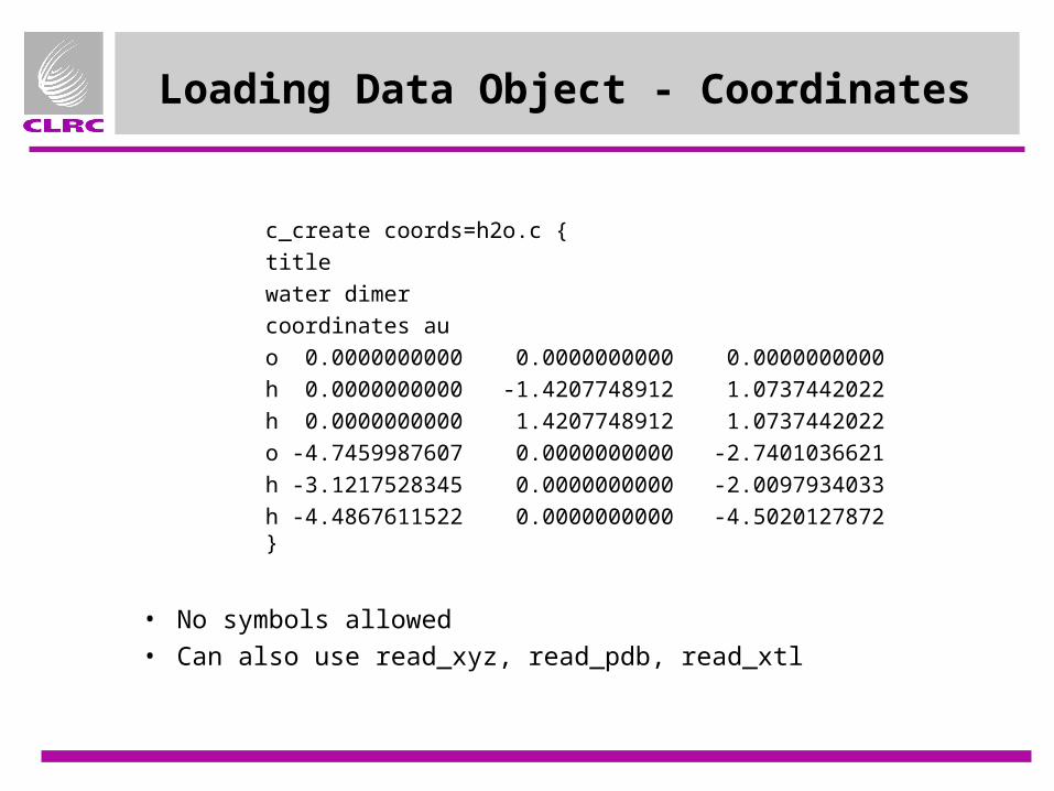
c_create coords=h2o.c {titlewater dimercoordinates auo 0.0000000000 0.0000000000 0.0000000000h 0.0000000000 -1.4207748912 1.0737442022h 0.0000000000 1.4207748912 1.0737442022o -4.7459987607 0.0000000000 -2.7401036621h -3.1217528345 0.0000000000 -2.0097934033h -4.4867611522 0.0000000000 -4.5020127872}
• No symbols allowed• Can also use read_xyz, read_pdb, read_xtl
Periodic Systems (i)
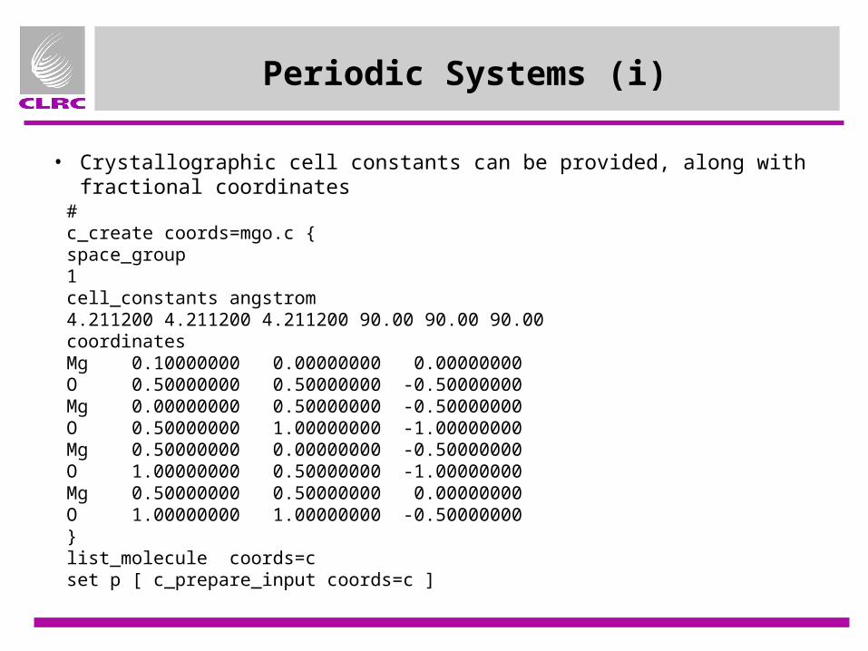
#c_create coords=mgo.c {space_group1cell_constants angstrom4.211200 4.211200 4.211200 90.00 90.00 90.00coordinatesMg 0.10000000 0.00000000 0.00000000O 0.50000000 0.50000000 -0.50000000Mg 0.00000000 0.50000000 -0.50000000O 0.50000000 1.00000000 -1.00000000Mg 0.50000000 0.00000000 -0.50000000O 1.00000000 0.50000000 -1.00000000Mg 0.50000000 0.50000000 0.00000000O 1.00000000 1.00000000 -0.50000000}list_molecule coords=cset p [ c_prepare_input coords=c ]
• Crystallographic cell constants can be provided, along with fractional coordinates

Periodic Systems (ii)
#c_create coords=d {titleprimitive unit cell of diamondcoordinates auc 0.8425347285 0.8425347285 0.8425347285c -0.8425347285 -0.8425347285 -0.8425347285cell au 0.00000 3.37014 3.37014 3.37014 0.00000 3.37014 3.37014 3.37014 0.00000}extend_fragment coords=d cell_indices= { -2 2 -2 2 -2 2 } result=d2
set_cell coords=d cell= { 0.00000 3.37014 3.37014 3.37014 0.00000 3.37014 3.37014 3.37014 0.00000 }
• Alternatively, input the cell explicitly, in c_create or attach to the structure later

QM Code Interfaces
• Provides access to third party codes ¤ GAMESS-UK¤ MOPAC ¤ MNDO¤ TURBOMOLE¤ Gaussian98
• Standardised interfaces¤ argument structure
• hamiltonian (includes functional)• charge, mult, scftype• basis (internal library or keywords)• accuracy• direct• symmetry• maxcyc...
energy coords=c \ theory=gamess : { basis=dzp hamiltonian=b3lyp } \ energy=e
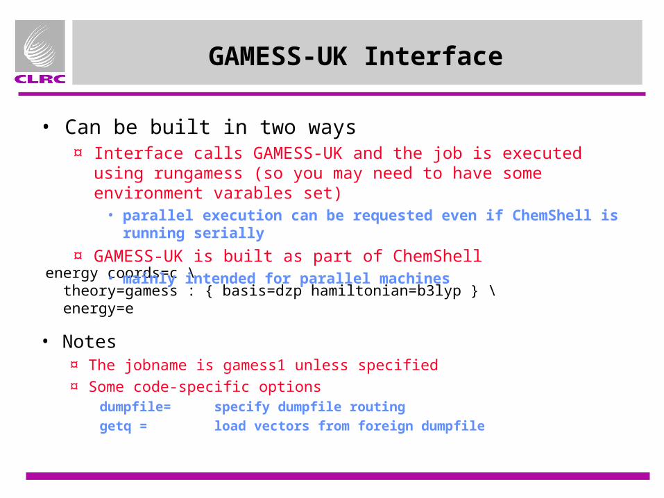
• Notes¤ The jobname is gamess1 unless specified¤ Some code-specific options
dumpfile= specify dumpfile routing
getq = load vectors from foreign dumpfile
GAMESS-UK Interface
• Can be built in two ways¤ Interface calls GAMESS-UK and the job is executed using rungamess (so
you may need to have some environment varables set) • parallel execution can be requested even if ChemShell is running serially
¤ GAMESS-UK is built as part of ChemShell• mainly intended for parallel machines
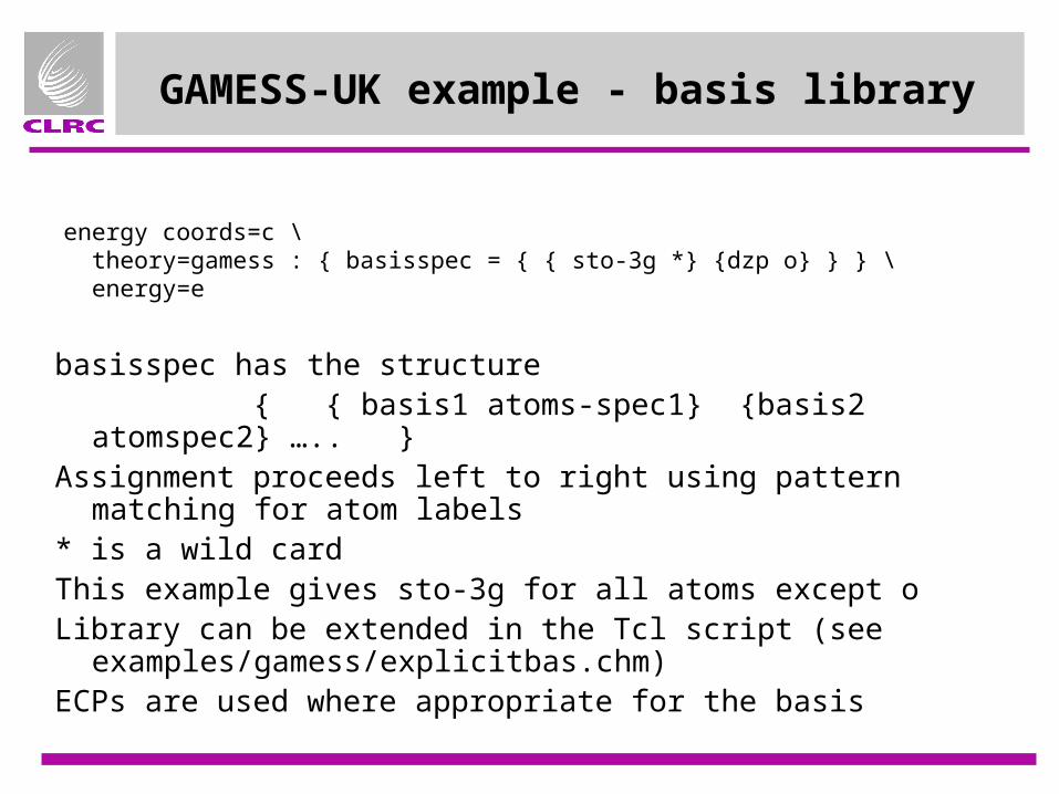
GAMESS-UK example - basis library
basisspec has the structure { { basis1 atoms-spec1} {basis2 atomspec2} ….. } Assignment proceeds left to right using pattern matching for atom
labels* is a wild cardThis example gives sto-3g for all atoms except oLibrary can be extended in the Tcl script (see
examples/gamess/explicitbas.chm)ECPs are used where appropriate for the basis
energy coords=c \ theory=gamess : { basisspec = { { sto-3g *} {dzp o} } } \ energy=e

DL_POLY Interface
• Features¤ Energy and gradient routines from DL_POLY (Bill Smith UK, CCP5)¤ General purpose MM energy expression, including approximations to
• CFF91 (e.g. zeolites)
• CHARMM
• AMBER
• MM2
¤ Topology generator • automatic atom typing
• parameter assignment based on connectivity
• topology from CHARMM PSF input
¤ FIELD, CONFIG, CONTROL are generated automatically¤ FIELD is built up using terms defined in the file specified by mm_defs= argument¤ Periodic boundary conditions are limited to parallelopiped shaped cells¤ Can have multiple topologies active at one time
DL_POLY forcefield terms
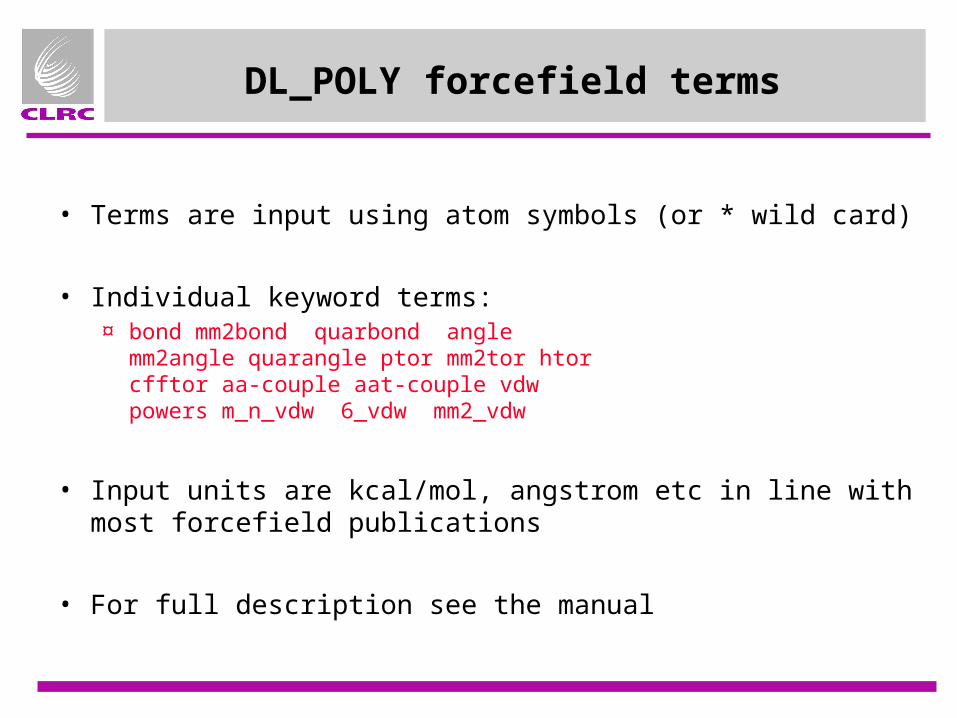
• Terms are input using atom symbols (or * wild card)
• Individual keyword terms:¤ bond mm2bond quarbond angle
mm2angle quarangle ptor mm2tor htor cfftor aa-couple aat-couple vdw powers m_n_vdw 6_vdw mm2_vdw
• Input units are kcal/mol, angstrom etc in line with most forcefield publications
• For full description see the manual

Automatic atom type assigment
• Forcefield definition can incorporate connectivity-based atom type definitions which will be used to assign types
• Atom types are hierarchical, most specific applicable type will be used (algorithm is iterative)
• e.g. to use different parameters for ipso-C of PPh3 define a new type by a connection to phosphorous
query ci "ipso c"supergroup ctarget catom pconnect 1 2endquery
charge c -0.15charge h 0.15
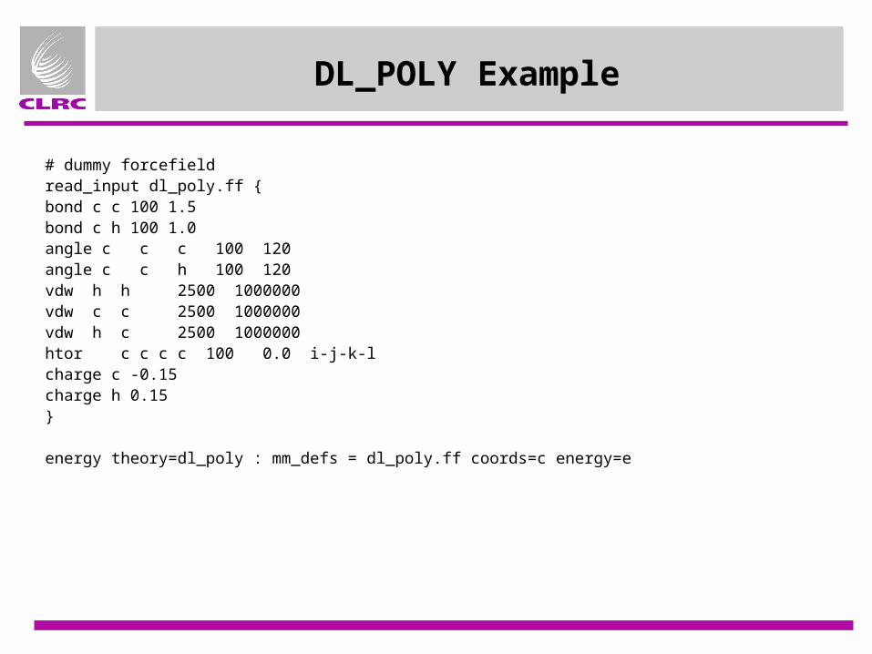
DL_POLY Example
# dummy forcefieldread_input dl_poly.ff {bond c c 100 1.5bond c h 100 1.0angle c c c 100 120angle c c h 100 120vdw h h 2500 1000000vdw c c 2500 1000000vdw h c 2500 1000000htor c c c c 100 0.0 i-j-k-lcharge c -0.15charge h 0.15}
energy theory=dl_poly : mm_defs = dl_poly.ff coords=c energy=e

Using DL_POLY with CHARMM Parameters
• Replicates CHARMM energy expression (without UREY)• Uses standard CHARMM datafiles• Requires CHARMM program + script to run as far as energy evaluation for initial setup • Atom charges and atom types are obtained by communication with a running CHARMM
process (usually only run once)
# run charmm using script providedcharmm.preinit charmm_script=all.charmm coords=charmm.c# Store type names from the topology fileload_charmm_types2 top_all22_prot.inp charmm_types
# These requires CTCL (i.e. charmm running)set types [ get_charmm_types ]set charges [ get_charmm_charges ]set groups [ get_charmm_groups ]#charmm.shutdown
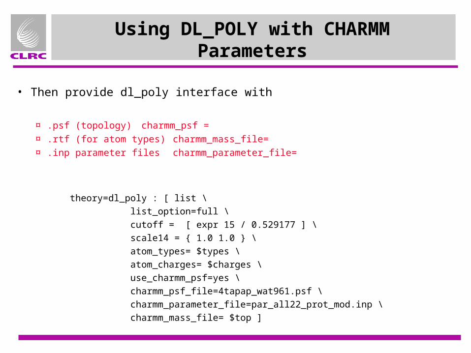
Using DL_POLY with CHARMM Parameters
theory=dl_poly : [ list \ list_option=full \ cutoff = [ expr 15 / 0.529177 ] \ scale14 = { 1.0 1.0 } \ atom_types= $types \ atom_charges= $charges \ use_charmm_psf=yes \ charmm_psf_file=4tapap_wat961.psf \ charmm_parameter_file=par_all22_prot_mod.inp \ charmm_mass_file= $top ]
• Then provide dl_poly interface with
¤ .psf (topology) charmm_psf =¤ .rtf (for atom types) charmm_mass_file=¤ .inp parameter files charmm_parameter_file=

Core modules: Geometry Optimisers
Small Molecules• Internal coordinates (delocalised,
redundant etc)• Full Hessian• O(N3) cost per step
¤ BFGS, P-RFO
Macromolecules• Cartesian coordinates• Partial Hessian (e.g. diagonal)• O(N) cost per step
¤ Conjugate gradient¤ L-BFGS
Coupled QM/MM schemes¤ Combine cartesian and internal coordinates
¤ Reduce cost of manipulating B, G matrices¤ Define subspace (core region) and relax environment at each step
¤ reduce size of Hessian ¤ exploit greater stability of minimisation vs. TS algorithms¤ Use approximate scheme for environmental relaxation

QUASI - Geometry Optimisation Modules
newopt¤ A general purpose optimiser
• Target functions, specified by function = – copt : cartesian (obsolete)– zopt: z-matrix (now also handles cartesians)– new functions can be written in Tcl (see example rosenbrock)
• For QM/MM applications e.g.– P-RFO adapted for presence of soft modes– Hessian update includes partial finite difference in eigenmode basis
• New algorithms can be coded in Tcl using primitive steps (forces, updates, steps, etc).
hessian¤ Generates hessian matrices (e.g. for TS searching)

Newopt example - minimisation
## function zopt allows the newopt optimiser to work with# the energy as a function of the internal coordinates of# the molecule#
newopt function=zopt : { theory=gamess : { basis=dzp } } \ zmatrix=z

Newopt example - transition state determination
# functions zopt.* allow the newopt optimiser to work with# the energy as a function of the internal coordinates of# the molecule
set args "{theory=gamess : { basis=3-21g } zmatrix=z}"
hessian function=zopt : [ list $args ] \ hessian=h_fcn_ts method=analytic
newopt function=zopt : [ list $args ] \ method=baker \ input_hessian=h_fcn_ts \ follow_mode=1

HDLCopt optimiser
hdlcopt ¤ Hybrid Delocalised Internal Coordinate scheme (Alex Turner, Walter
Thiel, Salomon Billeter) • Developed within QUASI project• O(N) overall scaling per step
¤ Key elements:
¤ Residue specification, often taken from a pdb file (pdb_to_res) allows separate delocalised coordinates to be generated for each residue
¤ Can perform P-RFO TS search in the first residue with relaxation of the others
• increased stability for TS searching• Much smaller Hessians
¤ Further information on algorithm• S.R. Billeter, A.J. Turner and W. Thiel, PCCP 2000, 2, p 2177

HDLCopt example
# procedure to update the last step
proc hdlcopt_update { args } { parsearg update { coords } $args write_xyz coords= $coords file=update.xyz end_module}
# select residuesset residues [ pdb_to_res "4tapap_wat83.pdb" ]# load coordinatesread_pdb file=4tapap_wat83.pdb coords=4tapap_wat83.c
hdlcopt coords=4tapap_wat83.c result=4tapap_wat83.opt \ theory=mndo : { hamiltonian=am1 charge=1 optstr={ nprint=2
kitscf=200 } } \ memory=200 residues= $residues \ update_procedure=hdlcopt_update

GULP Interface
• Simple interface to GULP energy and forces
• GULP licensing from Julian Gale
• GULP must be compiled in¤ in alpha version only for the workshop
• ChemShell fragment object supports shells¤ Shells are relaxed by GULP with cores fixed, ChemShell typically controls
the core positions
• Provide forcefield in standard GULP format

GULP interface example
read_input gulp.ff {# from T.S.Bush, J.D.Gale, C.R.A.Catlow and P.D. Battle# J. Mater Chem., 4, 831-837 (1994)speciesLi core 1.000Na core 1.000...buckinghamLi core O shel 426.480 0.3000 0.00 0.0 10.0Na core O shel 1271.504 0.3000 0.00 0.0 10.0...springMg 349.95Ca 34.05...}add_shells coords=mgo.c symbols= {O Mg}newopt function=copt : [ list coords=mgo.c theory=gulp : [ list
mm_defs=gulp.ff ] ]
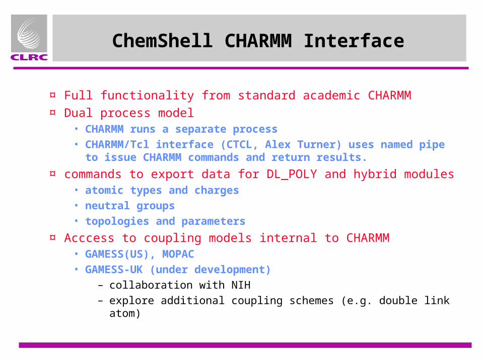
ChemShell CHARMM Interface
¤ Full functionality from standard academic CHARMM
¤ Dual process model• CHARMM runs a separate process • CHARMM/Tcl interface (CTCL, Alex Turner) uses named pipe to issue
CHARMM commands and return results.
¤ commands to export data for DL_POLY and hybrid modules• atomic types and charges• neutral groups• topologies and parameters
¤ Acccess to coupling models internal to CHARMM• GAMESS(US), MOPAC• GAMESS-UK (under development)
– collaboration with NIH– explore additional coupling schemes (e.g. double link atom)
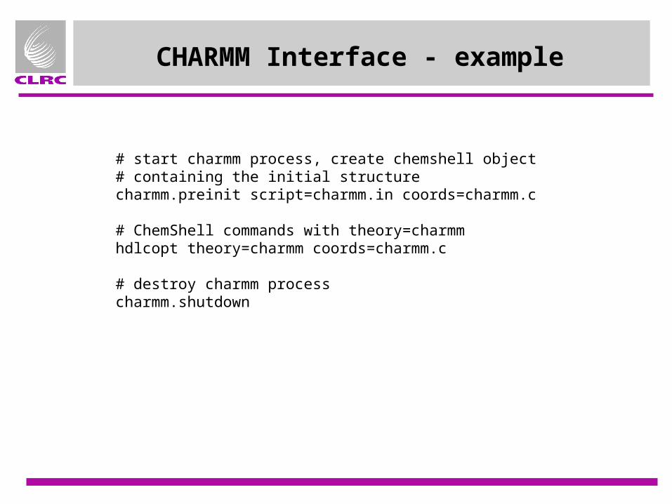
CHARMM Interface - example
# start charmm process, create chemshell object# containing the initial structurecharmm.preinit script=charmm.in coords=charmm.c
# ChemShell commands with theory=charmmhdlcopt theory=charmm coords=charmm.c
# destroy charmm processcharmm.shutdown

Molecular Dynamics Module
• Design Features¤ Generic - can integrate QM, MM, QM/MM trajectories
¤ Based on DL_POLY routines• Integration by Verlet leap-frog• SHAKE constraints• Quaternion rigid body motion• NVT, NPT, NVE integration
¤ Script-based control of primitive steps• Simulation Protocols
– equilibration– simulated annealing
• Tcl access to ChemShell matrix and coordinate objects– e.g. force modification for harmonic restraint
• Data output– trajectory output, restart files

Molecular Dynamics - arguments
• Object oriented syntax follows Tk etc¤ dynamics dyn1 coords=c … etc
• Arguments¤ theory= module used to compute energy and forces¤ coords= initial configuration of the system¤ timestep= integration timestep (ps) [0.0005] ¤ temperature= simulation temperature (K) [293]¤ mcstep= Max step displacement (a.u.) for Monte Carlo [0.2] ¤ taut= Tau(t) for Berendsen Thermostat (ps) [0.5]¤ taup= Tau(p) for Berendsen Barostat (ps) [5.0]¤ compute_pressure= Whether to compute pressure and virial (for NVT
simulation)¤ verbose= Provide additional output¤ energy_unit= Unit for output

Molecular dynamic - arguments
• Arguments (cont.)¤ rigid_groups= rigid group (quaternion defintions)
¤ constraints= interatomic distances for SHAKE
¤ ensemble= Choice of ensemble [NVE]
¤ frozen= List of frozen atoms
¤ trajectory_type= Additional fields for trajectory (> 0 for velocity, > 1 for forces)
¤ trajectory_file= dynamics.trj file for trajectory output
• Methods:¤ Dyn1 configure temperature=300
• configure - modify simulation parameters • initvel - initialise random velocities • forces - evaluate molecular forces • step - Take MD step
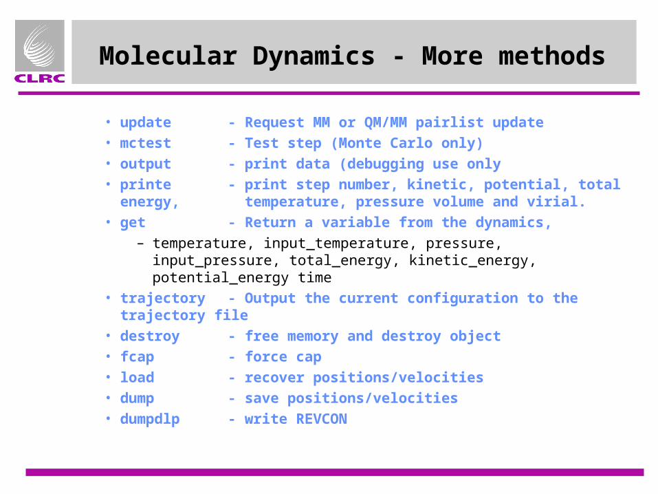
Molecular Dynamics - More methods
• update - Request MM or QM/MM pairlist update • mctest - Test step (Monte Carlo only) • output - print data (debugging use only • printe - print step number, kinetic, potential, total energy,
temperature, pressure volume and virial. • get - Return a variable from the dynamics,
– temperature, input_temperature, pressure, input_pressure, total_energy, kinetic_energy, potential_energy time
• trajectory - Output the current configuration to the trajectory file • destroy - free memory and destroy object• fcap - force cap• load - recover positions/velocities• dump - save positions/velocities• dumpdlp - write REVCON

Molecular Dynamics - Example
dynamics dyn1 coords=c theory=mndo temperature=300 timestep=0.005dyn1 initvelset nstep 0while {$nstep < 10000 } { dyn1 force dyn1 step ..... # additional Tcl commands here incr nstep}dyn1 configure temperature=300# etcdyn1 destroy
Hybrid Module
• All control data held in Tcl lists created¤ by setup program (Z-matrix style input)¤ by scripts or GUI etc¤ from user-supplied list of QM atoms provided as an argument
• Implements¤ Book-keeping
• Division of atom lists• addition of link atoms• summation of energy/forces
¤ Charge shift, and addition of a compensating dipole at M2
¤ Force resolution when link atoms are constrained to bond directions,e.g. the force on first layer MM atom (M1) arising from the force on the link atom is evaluated:
¤ Uses neutral group cutoff for QM/MM interactions
E
x
E
x
x
xM L
L
M1 1

Hybrid Module
• Typical input options¤ qm_theory=
¤ mm_theory=
¤ qm_region = { } list of atoms in the QM region
¤ coupling = type of coupling
¤ groups = { } neutral charge groups
¤ cutoff = QM/MM cutoff
¤ atom_charges = MM charges
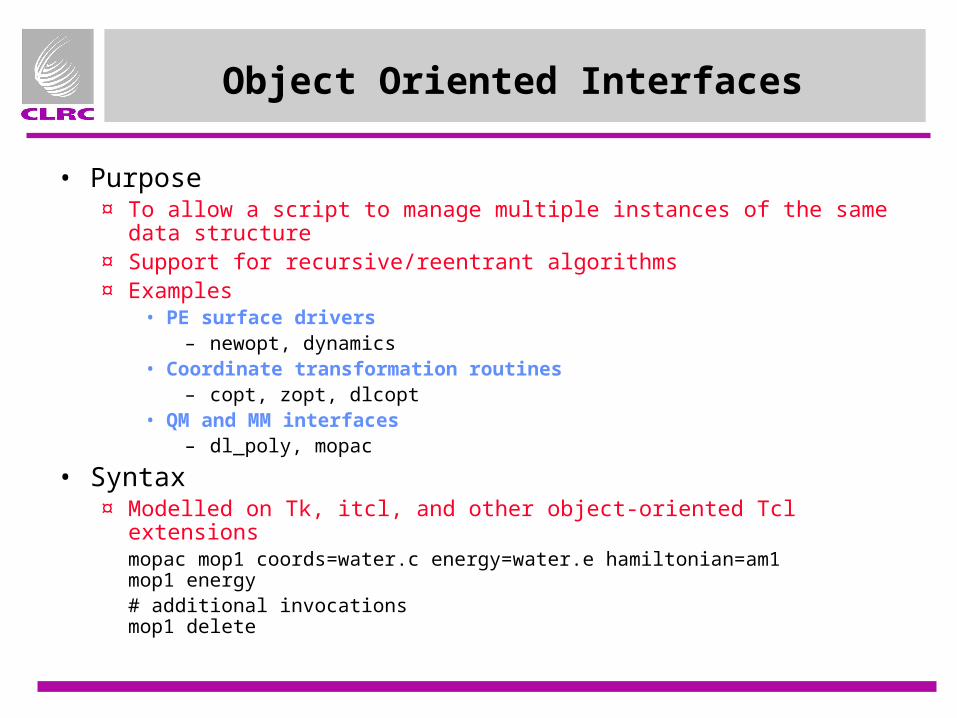
Object Oriented Interfaces
• Purpose¤ To allow a script to manage multiple instances of the same data structure ¤ Support for recursive/reentrant algorithms¤ Examples
• PE surface drivers– newopt, dynamics
• Coordinate transformation routines– copt, zopt, dlcopt
• QM and MM interfaces– dl_poly, mopac
• Syntax¤ Modelled on Tk, itcl, and other object-oriented Tcl extensions mopac mop1 coords=water.c energy=water.e hamiltonian=am1
mop1 energy# additional invocations
mop1 delete

Using multiple objects - A QM/MM optimisation scheme
zopt1
zopt2
newopt1
hopt
newopt2
dl_poly2
hybriddl_poly1
mopac
Object types
newopt: optimiser object
zopt: Z-matrix/cartesian transformation
dl_poly: MM energy and forces
hopt: Custom written target function (150 lines of Tcl)
Instances
zopt1: reduced (active site) coordinates
zopt2: environment coordinates
newopt1: master optimisation, QM/MM hamiltonian, in a reduced coordinate space
newopt2: relax the environment using a pure MM energy expression

• [1]• [2] A. Warshel, M. Levitt, J. Mol. Biol. 103 (1976) 227.• [3] J. Aqvist, A. Warshel, Chem. Rev. 93 (1993) 2523-44.• [4] J. Gao, in K.B. Lipkowitz, D.B. Boyd (Eds.), Reviews in Computational Chemistry. VCH, New York, 1995, vol. 7, p. 119.• [5] T.Z. Mordasini, W. Thiel, Chimia 52 (1998) 288-91.• [6] P. Sherwood, in J. Grotendorst (Ed.), Modern Methods and Algorithms in Quantum Chemistry. NIC Series, Jülich, 2000, vol., p. 257-77. http://www.fz-juelich.de/nic-series/Volume3/sherwood.pdf• [7] GAMESS-UK is a package of ab initio programs written by M.F. Guest, J.H. van Lenthe, J. Kendrick, K. Schöffel, and P. Sherwood, with contributions from R.D. Amos, R.J. Buenker, H.J.J. van Dam, M. Dupuis, N.C. Handy, I.H. Hillier, P.J. Knowles, V. Bonacic-Koutecky, W. von Niessen, R.J. Harrison, A.P. Rendell, V.R. Saunders, A.J. Stone, D.J. Tozer, and A.H. de Vries. The package is derived from the original GAMESS code due to M. Dupuis, D. Spangler and J. Wendoloski, NRCC Software Catalog, Vol. 1, Program No. QG01 (GAMESS), 1980. See http://www.dl.ac.uk/CFS.• [8] W. Thiel, MNDO99. Max-Planck-Institut für Kohlenforschung, Kaiser-Wilhelm-Platz 1, D-45470 Mülheim, Germany, 1999.• [9] P. Sherwood, A.H.de Vries, ChemShell User Manual, available online at http://www.cse.clrc.ac.uk/qcg/chemshell, 1997-2002.• [10] J.K. Ousterhout: Tcl and the Tk toolkit, Addison Wesley, 1994.• [11] W.L. DeLano, The PyMOL Molecular Graphics System (2002) on World Wide Web http://www.pymol.org.• [12] W. Smith, T. Forester, J. Mol. Graph. 14 (1996) 136.• [13] W. Smith, C.W. Yong, P.M. Rodger, Mol. Sim. 28 (2002) 385-471.• [14] J.R. Hill, J. Sauer, J. Phys. Chem. 99 (1995) 9536-50.• [15] J.R. Hill, J. Sauer, J. Phys. Chem. 98 (1994) 1238-44.• [16] B.R. Brooks, R.E. Bruccoleri, B.D. Olafson, D.J. States, S. Swaminathan, M. Karplus, J. Comput. Chem. 4 (1983) 187-217.• [17] J.D. Gale, J. Chem. Soc., Faraday Trans. 93 (1997) 629-37.• [18] B.G. Dick, A.W. Overhauser, Phys. Rev 112 (1958) 90.• [19] W.F.v. Gunsteren, S.R. Billeter, A.A. Eising, P.H. Hünenberger, P. Krüger, A.E. Mark, W.R.P. Scott, I.G. Tironi, Biomolecular Simulation: The GROMOS96 Manual and User Guide. Biomos, Zürich and Groningen, 1996.• [20] S.R. Billeter, C.F.W. Hanser, T.Z. Mordasini, M. Scholten, W. Thiel, W.F. van Gunsteren, Phys. Chem. Chem. Phys. 3 (2001) 688-95.• [21] S.P. Greatbanks, P. Sherwood, I.H. Hillier, J. Phys. Chem. 98 (1994) 8134-39.• [22] D. Das, K.P. Eurenius, E.M. Billings, P. Sherwood, D.C. Chatfield, M. Hodoscek, B.R. Brooks, J. Chem. Phys. 117 (2002) in press.• [23] P. Sherwood, A.H. de Vries, S.J. Collins, S.P. Greatbanks, N.A. Burton, M.A. Vincent, I.H. Hillier, Faraday Discuss. (1997) 79-92.• [24] W. Thiel, in J. Grotendorst (Ed.), Modern Methods and Algorithms in Quantum Chemistry. NIC Series, Jülich, 2000, vol., p. 233-55.
• [25] D. Bakowies, W. Thiel, J. Phys. Chem. 100 (1996) 10580-94.• [26] I. Antes, W. Thiel, J. Phys. Chem. A 103 (1999) 9290-95.• [27] R. Ahlrichs, M. Bär, M. Häser, H. Horn, C. Kölmel, Chem. Phys. Lett. 162 (1989) 165-69.• [28] C. Lennartz, A. Schäfer, F. Terstegen, W. Thiel, J. Phys. Chem. B 106 (2002) 1758-67.• [29] B. Paizs, G. Fogarasi, P. Pulay, J. Chem. Phys. 109 (1998) 6571-76.• [30] O. Farkas, H.B. Schlegel, J. Chem. Phys. 109 (1998) 7100-04.• [31] J. Baker, D. Kinghorn, P. Pulay, J. Chem. Phys. 110 (1999) 4986-91.• [32] K. Nemeth, O. Coulaud, G. Monard, J.G. Angyan, J. Chem. Phys. 114 (2001) 9747-53.• [33] S.R. Billeter, A.J. Turner, W. Thiel, Phys. Chem. Chem. Phys. 2 (2000) 2177-86.• [34] J. Baker, A. Kessi, B. Delley, J. Chem. Phys. 105 (1996) 192-212.• [35] F. Maseras, K. Morokuma, J. Comput. Chem. 16 (1995) 1170-79.• [36] A.J. Turner, V. Moliner, I.H. Williams, Phys. Chem. Chem. Phys. 1 (1999) 1323-31.• [37] Y.K. Zhang, H.Y. Liu, W.T. Yang, J. Chem. Phys. 112 (2000) 3483-92.• [38] M. Sierka, J. Sauer, J. Chem. Phys. 112 (2000) 6983-96.• [39] M. Bühl, F. Terstegen, F. Löffler, B. Meynhardt, S. Kierse, M. Müller, C. Näther, U. Lüning, Eur. J. Org. Chem. (2001) 2151-60.• [40] U. Eichler, C.M. Kölmel, J. Sauer, J. Comput. Chem. 18 (1997) 463-77.• [41] M. Sierka, J. Sauer, Faraday Discuss. (1997) 41-62.• [42] D. Nachtigallova, P. Nachtigall, M. Sierka, J. Sauer, Phys. Chem. Chem. Phys. 1 (1999) 2019-26.• [43] U.C. Singh, P.A. Kollman, J. Comput. Chem. 7 (1986) 718-30.• [44] M.J. Field, P.A. Bash, M. Karplus, J. Comput. Chem. 11 (1990) 700-33.• [45] D.M. Philipp, R.A. Friesner, J. Comput. Chem. 20 (1999) 1468-94.• [46] P.L. Cummins, J.E. Gready, Chem. Phys. Lett. 225 (1994) 11-17.• [47] D. Bakowies, W. Thiel, J. Comput. Chem. 17 (1996) 87-108.• [48] B.T. Thole, Chem. Phys. 59 (1981) 341-50.• [49] I. Antes, W. Thiel, in J.L. Gao, M.A. Thompson (Eds.), Combined Quantum Mechanical and Molecular Mechanical Methods. ACS Symp. Ser., 1998, vol. 712, p. 50.• [50] B.T. Thole, P.T.v. Duijnen, Theor. Chim. Acta 55 (1980) 307.• [51] M.A. Thompson, G.K. Schenter, J. Phys. Chem. 99 (1995) 6374-86.• [52] M.A. Thompson, J. Phys. Chem. 100 (1996) 14492-507.• [53] P.T. van Duijnen, F. Grozema, M. Swart, J. Mol. Struct. (THEOCHEM) 464 (1999) 191-98.• [54] P.E. Smith, W.F. van Gunsteren, in P.K. Weiner, A.J. Wilkinson (Eds.), Computer Simulation of Biomolecular Systems. ESCOM, Leiden, 1993, vol. 2, p. 182-212.• [55] L.N. Kantorovich, J. Phys. C 21 (1988) 5041-56.• [56] L.N. Kantorovich, Int. J. Quantum Chem. 78 (2000) 306-30.• [57] L.N. Kantorovich, Int. J. Quantum Chem. 76 (2000) 511-34.• [58] R. McWeeny: Methods of Molecular Quantum Mechanics, 2nd Edition, Academic Press, London, 1992.• [59] J.H. Lii, N.L. Allinger, J. Comput. Chem. 12 (1991) 186-99.• [60] I. Antes: PhD thesis, University of Zurich, 1998.• [61] B. Waszkowycz, I.H. Hillier, N. Gensmantel, D.W. Payling, J. Chem. Soc., Perkin Trans. 2 (1991) 1819-32.• [62] N. Reuter, A. Dejaegere, B. Maigret, M. Karplus, J. Phys. Chem. A 104 (2000) 1720-35.• [63] J.H. Harding, A.H. Harker, P.B. Keegstra, R. Pandey, J.M. Vail, C. Woodward, Physica B & C 131 (1985) 151-56.• [64] A.B. Kunz, J.M. Vail, Phys. Rev. B 38 (1988) 1058-63.• [65] J.M. Vail, R. Pandey, A.B. Kunz, Rev. Solid State Sci. 5 (1991) 241.• [66] A.L. Shluger, E.A. Kotomin, L.N. Kantorovich, J. Phys. C 19 (1986) 4183-99.• [67] A.L. Shluger, A.H. Harker, V.E. Puchin, N. Itoh, C.R.A. Catlow, Modell. Simul. Mater. Sci. Eng. 1 (1993) 673-92.• [68] A.L. Shluger, J.D. Gale, Phys. Rev. B 54 (1996) 962-69.• [69] A.L. Shluger, P.V. Sushko, L.N. Kantorovich, Phys. Rev. B 59 (1999) 2417-30.• [70] P.V. Sushko, A.L. Shluger, C.R.A. Catlow, Surf. Sci. 450 (2000) 153-70.• [71] J.S. Braithwaite, P.V. Sushko, K. Wright, C.R.A. Catlow, J. Chem. Phys. 116 (2002) 2628-35.• [72] S. Huzinaga, L. Seijo, Z. Barandiaran, M. Klobukowski, J. Chem. Phys. 86 (1987) 2132-45.• [73] L. Seijo, Z. Barandiaran, J. Math. Chem. 10 (1992) 41-56.• [74] M.A. Nygren, L.G.M. Pettersson, Z. Barandiaran, L. Seijo, J. Chem. Phys. 100 (1994) 2010-18.• [75] L. Seijo, Z. Barandiaran, Int. J. Quantum Chem. 60 (1996) 617-34.• [76] J.L. Pascual, L. Seijo, J. Chem. Phys. 102 (1995) 5368-76.• [77] M. Born, Huang: Dynamical Theory of Crystal Lattices, Oxford: Oxford University Press, 1954.• [78] G. Venkataraman, L.A. Feldkamp, V.C. Sahni: Dynamics of Perfect Crystals, MIT: Cambridge, 1975.• [79] T.J. Grey, J.D. Gale, D. Nicholson, Mol. Phys. 98 (2000) 1565-73.• [80] M.S.D. Read, M.S. Islam, F. King, F.E. Hancock, J. Phys. Chem. B 103 (1999) 1558-62.• [81] L. Whitmore, A.A. Sokol, C.R.A. Catlow, Surf. Sci. 498 (2002) 135-46.• [82] P.J. Hay, W.R. Wadt, J. Chem. Phys. 82 (1985) 270-83.• [83] P.J. Hay, W.R. Wadt, J. Chem. Phys. 82 (1985) 299-310.• [84] W.R. Wadt, P.J. Hay, J. Chem. Phys. 82 (1985) 284-98.• [85] P. Durand, J.C. Berthelat, Theor. Chim. Acta 38 (1975) 283.• [86] M. Dolg, U. Wedig, H. Stoll, H. Preuss, J. Chem. Phys. 86 (1987) 866-72.• [87] J. Nieplocha, R.J. Harrison, R.J. Littlefield, J. Supercomputing 10 (1996) 197-220.• [88] M. Bowker, Vacuum 33 (1983) 669-85.• [89] S. Bailey, G.F. Froment, J.W. Snoeck, K.C. Waugh, Catal. Lett. 30 (1995) 99-111.• [90] S.A. French, A.A. Sokol, S.T. Bromley, C.R.A. Catlow, S.C. Rogers, F. King, P. Sherwood, Angew. Chem.-Int. Edit. 40 (2001) 4437.• [91] D.H. Gay, A.L. Rohl, J. Chem. Soc., Faraday Trans. 91 (1995) 925-36.• [92] R. Krishnan, J.S. Binkley, R. Seeger, J.A. Pople, J. Chem. Phys. 72 (1980) 650.• [93] A.D. McLean, G.S. Chandler, J. Chem. Phys. 72 (1980) 5639.• [94] T.H. Dunning, J. Chem. Phys. 90 (1989) 1007-23.• [95] R.A. Kendall, T.H. Dunning, R.J. Harrison, J. Chem. Phys. 96 (1992) 6796-806.• [96] F. Kapteijn, J. RodriguezMirasol, J.A. Moulijn, Appl. Catal., B 9 (1996) 25-64.• [97] Y.J. Li, J.N. Armor, Appl. Catal., B 1 (1992) L21-L29.• [98] G. Kresse, J. Hafner, Phys. Rev. B 47 (1993) 558-61.• [99] G. Kresse, J. Hafner, Phys. Rev. B 49 (1994) 14251-69.• [100] G. Kresse, J. Furthmuller, Comput. Mater. Sci. 6 (1996) 15-50.• [101] W.F. Schneider, K.C. Hass, R. Ramprasad, J.B. Adams, J. Phys. Chem. B 102 (1998) 3692-705.• [102] W.F. Schneider, K.C. Hass, R. Ramprasad, J.B. Adams, J. Phys. Chem. B 101 (1997) 4353-57.• [103] J.C. Schöneboom, H. Lin, N. Reuter, W. Thiel, S. Cohen, F. Ogliaro, S. Shaik, J. Am. Chem. Soc. 124 (2002) 8142-51.• [104] Q. Cui, M. Karplus, J. Am. Chem. Soc. 123 (2001) 2284-90.• [105] Q. Cui, M. Karplus, J. Phys. Chem. B 106 (2002) 1768-98.• [106] L. Ridder, A.J. Mulholland, J. Vervoort, I. Rietjens, J. Am. Chem. Soc. 120 (1998) 7641-42.• [107] W.J.H. van Berkel, F. Müller, Eur. J. Biochem. 179 (1989) 307-14.• [108] S. Thiel, W. Thiel, to be published.• [109] R. Davydov, T.M. Makris, V. Kofman, D.E. Werst, S.G. Sligar, B.M. Hoffman, J. Am. Chem. Soc. 123 (2001) 1403-15.• [110] I. Schlichting, J. Berendzen, K. Chu, A.M. Stock, S.A. Maves, D.E. Benson, B.M. Sweet, D. Ringe, G.A. Petsko, S.G. Sligar, Science 287 (2000) 1615-22.
P. Sherwood, in J. Grotendorst (Ed.), Modern Methods and Algorithms in Quantum Chemistry. NIC Series, Jülich, 2000, vol., p. 257-77. http://www.fz-juelich.de/nic-series/Volume3/sherwood.pdf