PUBLICATIONS - Scripps Institution of Oceanographysgille/pub_dir/jgrc20874.pdf · can indirectly affect SST by modulating upper ocean stratiﬁcation [Lukas and Lindstrom, 1991; de

RESEARCH ARTICLE10.1002/2014JC009924

The diurnal salinity cycle in the tropics

Kyla Drushka1,2, Sarah T. Gille1, and Janet Sprintall1

1Scripps Institution of Oceanography, University of California, San Diego, La Jolla, California, USA, 2Now at Applied PhysicsLaboratory, University of Washington, Seattle, Washington, USA

Abstract Observations from 35 tropical moorings are used to characterize the diurnal cycle in salinity at1 m depth. The amplitude of diurnal salinity anomalies is up to 0.01 psu and more typically �0.005 psu.Diurnal variations in precipitation and vertical entrainment appear to be the dominant drivers of diurnalsalinity variability, with evaporation also contributing. Areas where these processes are strong are expectedto have relatively strong salinity cycles: the eastern Atlantic and Pacific equatorial regions, the southwesternBay of Bengal, the Amazon outflow region, and the Indo-Pacific warm pool. We hypothesize that salinityanomalies resulting from precipitation and evaporation are initially trapped very near the surface and maynot be observed at the 1 m instrument depths until they are mixed downward. As a result, the pattern ofdiurnal salinity variations is not only dependent on the strength of the forcing terms, but also on the phas-ing of winds and convective overturning. A comparison of mixed-layer depth computed with hourly andwith daily averaged salinity reveals that diurnal salinity variability can have a significant effect on upperocean stratification, suggesting that representing diurnal salinity variability could potentially improve air-sea interaction in climate models. Comparisons between salinity observations from moorings and from theAquarius satellite (level 2 version 3.0 data) reveal that the typical difference between ascending-node anddescending-node Aquarius salinity is an order of magnitude greater than the observed diurnal salinityanomalies at 1 m depth.

1. Introduction

The diurnal cycle of salinity is important because it influences upper ocean stratification, which in turn affectssea surface temperature (SST) and air-sea fluxes of heat and momentum. Solar insolation varies throughoutthe day, which drives diurnal cycles in the upper ocean that include variations in temperature [Kawai andWada, 2007], momentum and shear [Cronin and Kessler, 2009], turbulence and mixed-layer depth [Lien et al.,1995]. Diurnal variability is increasingly thought to play an important role in the coupled air-sea system [Kawaiand Wada, 2007; Clayson and Bogdanoff, 2013]: models driven with subdaily forcing more accurately repro-duce oceanic and atmospheric variations at diurnal and intraseasonal time scales compared to those forcedwith daily fields [e.g., McCreary et al., 2001; Bernie et al., 2005; Woolnough et al., 2007]. Diurnal variations of tur-bulence and mixing at the base of the mixed layer also appear to modulate the downward transfer of energy[Woods et al., 1984; Danabasoglu et al., 2006], suggesting that diurnal variability may be important for theinteraction of the surface layer and the deeper ocean [Bernie et al., 2005]. Model sensitivity studies have shownthat a diurnally varying mixed layer is necessary in order to accurately reproduce intraseasonal (i.e., Madden-Julian Oscillation, MJO) variations. The formation of a diurnal warm layer results in a warmer daily-mean SST,which affects convection and winds; wind and convective anomalies associated with the MJO modulate theformation of diurnal warm layers [Bernie et al., 2005; Shinoda, 2005; Woolnough et al., 2007; Li et al., 2013].There are thus feedbacks between diurnal and intraseasonal air-sea processes in the tropics, illustrating theimportance of understanding what drives upper ocean stratification on diurnal scales. None of the studies ofdiurnal-intraseasonal feedbacks considered the role played by salinity. Since salinity controls upper oceanstratification throughout much of the tropics [Sprintall and Tomczak, 1992; de Boyer Mont�egut et al., 2007], itcan potentially play a role in the coupled air-sea system [Anderson et al., 1996]. Understanding where and whydiurnal salinity variations are strong will help to model this complex system.

Although the average diurnal sea surface salinity (SSS) cycle is likely small [�0.005 psu; Cronin and McPha-den, 1999], there are still good reasons for investigating the drivers of diurnal salinity variability. First, salinitycan indirectly affect SST by modulating upper ocean stratification [Lukas and Lindstrom, 1991; de Boyer

Special Section:Early scientific results from thesalinity measuring satellitesAquarius/SAC-D and SMOS

Key Points:� Diurnal salinity throughout the

tropics up to 0.01 psu� Diurnal entrainment and

precipitation drive diurnal salinity� Aquarius ascending-descending

difference exceeds day-night salinitysignal

Correspondence to:K. Drushka,[email protected]

Citation:Drushka, K., S. T. Gille, and J. Sprintall(2014), The diurnal salinity cycle in thetropics, J. Geophys. Res. Oceans, 119,5874–5890, doi:10.1002/2014JC009924.

Received 1 MAR 2014

Accepted 19 AUG 2014

Accepted article online 23 AUG 2014

Published online 10 SEP 2014

DRUSHKA ET AL. VC 2014. American Geophysical Union. All Rights Reserved. 5874

Journal of Geophysical Research: Oceans

PUBLICATIONS

http://dx.doi.org/10.1002/2014JC009924

http://onlinelibrary.wiley.com/journal/10.1002/(ISSN)2169-9291/specialsection/SACDSMOS/



http://onlinelibrary.wiley.com/journal/10.1002/(ISSN)2169-9291/

http://publications.agu.org/

Mont�egut et al., 2007], and hence the amount by which the sea surface warms and cools during the courseof a day [Soloviev and Lukas, 2006]. Understanding where and when diurnal salinity variations are large willallow us to assess their role in the coupled air-sea system, and will help guide decisions about whether sub-daily salinity variations should be included in models. Second, differences between the descending andascending nodes of the Aquarius satellite, which sample in the morning and evening, respectively, canintroduce a day-night bias in SSS retrievals. A knowledge of diurnal SSS variations will help unravel this bias.

Despite recent progress toward quantifying global near-surface salinity variations [e.g. Roemmich and Gilson,2009; Durack and Wijffels, 2010], the understanding of salinity variability on shorter timescales is still limited[Maes et al., 2013]. Quantifying the daily salinity cycle is a challenge: in contrast to SST, which is controlledby a fundamentally diurnal process—solar insolation—SSS is governed by several processes, including pre-cipitation, evaporation, and mixing, that are not exclusively driven by diurnal processes and are not neces-sarily in phase. An additional challenge is that precipitation-driven salinity anomalies often do notpenetrate more than 1 m into the water column [Henocq et al., 2010], which is above the shallowest depthmeasured from most in situ platforms such as typical Argo floats, ship-board thermosalinographs, orexpendable conductivity-temperature-depth probes. As a result, relatively few salinity observations that canbe used to characterize the diurnal cycle exist for the top meter of the ocean. The goal of the present studyis to determine where diurnal salinity variations are strong and to assess the forcing mechanisms that drivethese variations. We use data from moorings throughout the tropics to estimate the average diurnal cycleof 1 m salinity and of precipitation, evaporation, vertical entrainment, and horizontal advection. Findingsfrom this study may ultimately help to improve retrievals by the salinity satellite missions as well as guidefuture in situ and model sensitivity studies aimed at quantifying the role of diurnal salinity variations in thecoupled ocean-atmosphere system.

2. Background

2.1. Drivers of Diurnal SalinityDiurnal SST anomalies are largely driven by solar insolation, which peaks at roughly the same local time ateach day [Woods, 1980; Kawai and Wada, 2007]. In contrast, it is not obvious that salinity should vary diur-nally. While a handful of studies have documented strong changes in upper ocean salinity over the courseof several days or less [e.g. Anderson et al., 1996; Wijesekera and Gregg, 1996; Vialard et al., 2009], few haveevaluated whether those daily changes occur systematically, and, if so, what the implications might be interms of potential feedbacks to the atmosphere. Changes in the salinity averaged over the mixed layer (�S)can be described by:

@�S@t

5E2P

h�S|fflffl{zfflffl}

a

2 u � r�S|fflfflffl{zfflfflffl}b

2 wEDSh|fflffl{zfflffl}

c

1�; (1)

where E and P represent rates of evaporation and precipitation, respectively; h is the mixed-layer depth(MLD); u is the two-dimensional horizontal velocity; wE is the vertical entrainment velocity at the base of themixed layer; and DS represents the change in salinity across the base of the mixed layer. The terms on theright-hand side of equation (1) hence represent (a) surface forcing, (b) horizontal salt advection, and (c) ver-tical entrainment of salt at the base of the mixed layer. � represents horizontal and vertical diffusion andvertical advection. The relative amplitudes and phasing of these processes, as well as the background oceanstratification, all affect how surface salinity varies throughout the course of the day.

Diurnal precipitation is generally strongest in regions with strong mean rainfall, including the IntertropicalConvergence Zone in the Pacific and Atlantic Oceans, the eastern Indian Ocean north of the equator, thewestern Pacific Ocean, and near the coastlines in the western side of each ocean basin [Kikuchi and Wang,2008]. Rainfall in the tropics and subtropics typically peaks in the early morning to midmorning, with after-noon rain also common [Janowiak et al., 1994; Nesbitt and Zipser, 2003]. Tropical rainfall tends to be inter-mittent in space and time, leading to low-salinity surface patches [Soloviev and Lukas, 2006] that are mixedaway within hours to days, primarily due to nighttime convective overturning in the mixed layer [Brainerdand Gregg, 1997; Wijesekera et al., 1999]. Strong rain can produce a thin, buoyant halocline that suppressesturbulent exchange with the water below, trapping atmospheric fluxes to the near surface [Wijesekera et al.,

Journal of Geophysical Research: Oceans 10.1002/2014JC009924


1999]. The strong surface stratification produced by heavy rainfall also reduces the vertical entrainment ofsalt and heat [Anderson et al., 1996].

Wind drives evaporation, which increases SSS [Soloviev and Lukas, 1997, 2006], and also acts to break downsurface stratification and deepen the mixed layer. Wind tends to be strongest in the morning and eveningnear coastlines due to land-sea heat contrasts; the amplitude of the diurnal wind signal decays with dis-tance from shore, and the phasing is highly variable away from the coast [Gille et al., 2005]. In the tradewind bands of the Pacific and Atlantic Oceans, diurnal wind variations are moderately strong, though thephasing varies over small spatial scales (a few degrees of longitude and latitude) [Gille et al., 2005]. Evapora-tion is also affected by air and sea surface temperature and humidity [Fairall et al., 1996], which can varydiurnally. In addition to wind stress, convection that results from nighttime cooling at the sea surface causesthe mixed layer to deepen, entraining deeper water into the mixed layer. Entrainment can increase ordecrease surface salinity depending on the sign of the vertical salinity gradient (DS in equation (1)); salinityincreases with depth in most regions [e.g. de Boyer Mont�egut et al., 2007], so entrainment generally causesthe mixed layer to become more salty.

Diurnal warming can produce a stable daytime surface layer that traps momentum flux, enhancing surfacecurrents [e.g., Bernie et al., 2007; Cronin and Kessler, 2009]; in the presence of a horizontal salinity gradientr�S, this could produce diurnal salinity advection. We assume that this is the primary driver of any horizontalsalt advection, i.e., the horizontal salinity gradient does not vary systematically on diurnal time scales.Although diurnal variations in diffusive processes have been observed [e.g., Lien et al., 1995], we assumethat their impacts on near-surface salinity are negligible.

For equation (1) to hold true, salinity anomalies resulting from each of the processes on the right-hand side mustbe incorporated into the mixed layer on time scales at least as fast as the equation is evaluated: in this case,hours. However, it actually takes hours or longer for precipitation anomalies to be distributed throughout themixed layer: rain forms thin, stable surface lenses that disperse within a few hours due to mixing, diffusion, and/or advection [Brainerd and Gregg, 1997; Wijesekera et al., 1999; Tomczak, 1995]. For a given rain event, the depthof the resulting fresh lens depends on the strength and duration of the rainfall and the local wind speed [Miller,1976] as well as the size of the rain drops [Katsaros and Buettner, 1969]. Early laboratory experiments showed rainpenetrating to<10 cm; observational studies have revealed rain-formed lenses ranging in thickness from tens ofcentimeters [McCulloch et al., 2012; Reverdin et al., 2012] to meters [Price, 1979; Soloviev and Lukas, 2006] to over10 m [Wijesekera et al., 1999]. The depth to which evaporation modulates near-surface salinity is not well under-stood because it is so difficult to measure [Yu, 2010], and few studies have presented observations of near-surface salinity anomalies resulting from evaporation. For example, Soloviev and Vershinsky [1982] observed a�0.02 psu salinity increase in the top 0.5 m that may have been caused by evaporation, but the uncertainty onthe measurement was as large as the signal. More recently, Asher et al. [2014a], using a towed surface salinity pro-filer, found salt-enhanced surface lenses around 0.5 m thick in the subtropical North Atlantic. They noted thatmoderate winds are needed to evaporate enough water to produce a measureable surface salinity anomaly, butwinds stronger than a few m s21 destroy the ability of the surface to support salty anomalies.

A modified version of equation (1) is thus needed to explain salinity anomalies at a discrete depth on timescales faster than 1 day. For an instrument at a depth of 1 m, the salinity change dS1 measured during ashort time step dt (e.g., dt51 h) can be approximated by the following:

dS1 �ð

EhE

S1dt2ð

PhP

S1dt2ð

u1 � rS1dt2dhDS

h: (2)

Equation (2) takes into account the depth to which salinity anomalies resulting from precipitation and evapo-ration penetrate prior to being mixed or advected away, denoted hP and hE, respectively. When hE or hP arethinner than 1 m (and hence the associated salinity anomaly is not detected at 1 m depth), the evaporation orprecipitation term is set to zero. Vertical entrainment is assumed to result from the mixed layer deepening byan amount dh, so vertical velocity is approximated as dh/dt; the associated salinity anomaly is assumed to bedistributed throughout the mixed layer and hence is scaled by MLD (h). Horizontal advection is assumed toresult from the near-surface current u1 acting on the background horizontal salinity gradientrS1.

Results from previous studies examining diurnal salinity cycles have suggested that vertical entrainment may bethe dominant driver of diurnal SSS: Cronin and McPhaden [1999] used 1 m data from several TOGA-COARE



moorings in the western Pacific Ocean to show a 60.005 psu daily salinity cycle with a maximum in the earlymorning, despite strong local rainfall at that time. They suggested that nighttime surface cooling drives over-turning in the mixed layer and entrains deeper, saltier water, producing the early morning salinity maximum.Cronin and McPhaden [1999] also showed that the diurnal salinity signal at 3 m depth was substantially weakerthan that at 1 m depth. Reverdin et al. [2012] showed the average daily salinity cycle in two tropical regionsbased on data from surface drifters at 15–50 cm depth. In the southwest tropical Pacific Ocean, they found anearly morning salinity minimum (i.e., a signal with opposite phasing to that observed by Cronin and McPhaden[1999]) and suggested that strong nighttime rainfall increases surface stability and hence reduces verticalentrainment. Though the studies of Cronin and McPhaden [1999] and Reverdin et al. [2012] found systematicdiurnal salinity cycles, in both cases, the statistical uncertainties on the estimates were nearly as large as the sig-nals themselves. Recently, J. E. Anderson and S. C. Riser (Near-surface variability of temperature and salinity inthe near-tropical ocean: Observations from profiling floats, submitted to Journal of Geophysics Research, 2014)used specialized Argo floats that profile to within�0.2 m of the sea surface to quantify the diurnal cycle ofnear-surface salinity in several regions. They showed a diurnal salinity anomaly on the order of 0.1 psu at 0.2 mdepth, which is smaller by an order of magnitude at 1 m depth, roughly consistent with the result of Cronin andMcPhaden [1999]. To our knowledge, these are the only studies that have considered systematic diurnal salinityanomalies. Their findings highlight the following hypotheses: (a) the phasing and amplitude of diurnal SSS varyspatially; (b) vertical entrainment at the base of the mixed layer is an important driver of diurnal SSS variations;(c) day-to-day variability in subdaily salinity may smooth the average diurnal signal; and (d) diurnal salinity varia-tions decrease substantially with depth, even within the top tens of centimeters of the water column. In thepresent study, we use salinity data at 1 m depth from moorings to assess these hypotheses.

3. Data and Methods

3.1. MooringsWe used data from moorings in the Tropical Atmosphere Ocean (TAO) mooring array, which aredistributed by the TAO Project Office of the Pacific Marine Environmental Laboratory (PMEL) at the NationalOceanic and Atmospheric Administration (NOAA). Only the data with the highest level of accuracy (qualitycontrol flags 1 or 2) were used. At 47 mooring sites, at least 1 year of hourly salinity data (>8760 datapoints) were available; an additional 24 moorings had hourly salinity with <1 year of high-quality data.Where available, we also utilized other hourly measurements made at the moorings: precipitation andwinds (typically measured 4 m and 3.5 m above the sea surface, respectively); near-surface horizontal cur-rents at 10 m depth; and salinity and temperature at all available depths throughout the water column.Three moorings had hourly measurements of both temperature and salinity data with �10 m vertical spac-ing in the top 50 m; for those sites, MLD was computed using a density-threshold criterion: density wasinterpolated vertically to a 1 m grid and then MLD was defined as the depth at which density decreased by0.125 kg m23 relative to 1 m density. Nine of the TAO sites also had >1 year of hourly evaporation esti-mates, which were derived using the Coupled Ocean Atmosphere Response Experiment (COARE) 3.0b bulkflux algorithm [Fairall et al., 2003; Cronin et al., 2006]. Note that no single site had hourly precipitation, evap-oration, and MLD data.

To extract the average diurnal signal, the data were processed in a manner similar to that described by Croninand McPhaden [1999]. First, a low-pass Hamming filter with a 3 day cutoff was applied to the time series at eachmooring; this signal was removed, and the remaining high-frequency component was then smoothed with a1-2-1 triangle filter. The resulting anomalies were then binned according to the local hour of the measurement.For each hourly time bin, this gave an average salinity anomaly and its uncertainty, which was calculated as thestandard error, i.e., the standard deviation divided by the square root of the number of data points. Then, diurnaland semidiurnal harmonics were fit simultaneously using a weighted linear least-squares technique, where theuncertainty of the averages in each time bin provided the weighting. The minimum and maximum daily salinityanomalies were extracted from the fit, and amplitude was computed as half the difference between the maxi-mum and the minimum. The uncertainty of the fit was used to test the significance of the diurnal signals.

The length of the salinity time series varies between individual sites. Generally, diurnal averages made with longertime series have smaller amplitudes, likely as a result of unresolved low-frequency variations that smooth out thesignal when many data points are binned. To avoid biases resulting from differences in record length, we usedexactly 1 year of data from each site and rejected any sites that displayed interannual variability in the diurnal



salinity amplitude. This was done by breaking the full time series into distinct 1 year segments of data and com-puting the diurnal phase and amplitude for each segment. Sites for which the amplitude of the different segmentsvaried by more than 50% of the signal, or the diurnal phase for the different segments differed by more than 2 h,were excluded from the analysis: 12 sites from throughout the set of moorings were removed this way, leaving atotal of 35 mooring sites for which we were confident that the diurnal salinity anomalies could be computed.

3.2. Aquarius DataThe Aquarius satellite is in a polar sun-synchronous orbit and so sees the Earth at the same two times each day,crossing the equator at roughly 06:00 local time (descending nodes) and 18:00 (ascending nodes) [Lagerloefet al., 2008]. As a result, any uncorrectable noise that varies with the time of day or the direction of the satellitewill produce biases between the ascending and descending nodes of the orbit. For example, radio-frequencyinterference that is sampled at different look angles during ascending and descending nodes introduces a biasin some regions (G. Lagerloef, personal communication, 2014), which may mask ascending-descending differen-ces in surface salinity that arise from the actual diurnal salinity cycle. In section 5.2, we estimate the ascending-descending differences in Aquarius salinities. We use the Aquarius Level 2 Combined Active-Passive (CAP) V3.0data set, which has the most up-to-date (as of August 2014) ascending/descending bias corrections. Thisproduct was obtained from the NASA Physical Oceanography Distributed Active Archive Center (PO.DAAC). TheCAP algorithm corrects Aquarius radiometer measurements using simultaneous observations from the onboardscatterometer [Yueh, 2013]. The data set consists of along-track salinity and wind observations for each of thethree radiometers [Le Vine et al., 2007]. The satellite samples each 1.44 s, giving �9.5 km along-track measure-ment spacing; each orbit repeats every 7 days. Two years of Aquarius data, from January 2012 to December2013, were used in this study.

3.3. Ancillary DataWe used several additional data sets to evaluate the salinity observations in the context of atmospheric forc-ing and background ocean conditions. The Monthly Isopycnal and Mixed-layer Ocean Climatology (MIMOC)[Schmidtko et al., 2013] database provided information about the mean ocean stratification. This product isbased primarily on Argo profiling float data, and includes temperature and salinity at standard depth levels(5 m vertical resolution in the top 100 m), as well as MLD, on a monthly, 0.5� horizontal grid. Climatologicalzonal and meridional gradients of surface salinity were estimated using a central difference method.

Global observations of evaporation came from the Hamburg Ocean Atmosphere Parameters and Fluxes fromSatellite Data Set version 3.2 [HOAPSv3.2; Fennig et al., 2012] which is derived from Special Sensor MicrowaveImager (SSM/I) satellite data and is available as a 6 h composite on a 0.5� grid. Precipitation came from theTropical Rainfall Measuring Mission (TRMM) 3B42 version seven data set, which is produced from satellite-based radar, microwave, and visible infrared observations and is available on a 3 hourly, 0.25� horizontal grid[Huffman et al., 2007]. The evaporation and precipitation data sets were smoothed to a 1� spatial grid and thetimestamp for the data in each grid box was converted to local time based on its longitude. The diurnal cycleat each grid point was extracted using a methodology similar to that used for the mooring data: the timeseries were filtered to isolate high-frequency variations, then the 24 h harmonic was fit to the filtered data (asthese were 6 and 3 hourly fields, the semidiurnal harmonic was not included in the fit). This gave maps of thediurnal amplitude of evaporation and precipitation. Using 6 or 3 hourly data to compute the diurnal cyclelikely underestimates the signal; we thus use these diurnal amplitude maps as a way to assess where diurnalevaporation and precipitation are likely to be relatively strong rather than to produce high-accuracy estimatesof the diurnal variation of these processes. Finally, shortwave radiation, net heat flux, and wind stress from theTropFlux product were used to compute mean Monin-Obukhov length scales [e.g., Venkatram, 1980], whichcan be used to relate atmospheric conditions to properties of the mixed layer. TropFlux is computed usingthe COARE v3 bulk flux algorithm applied to a combination of ERA-I reanalysis ISCCP surface radiation, and isavailable on a daily, 1� grid throughout the tropics [Kumar et al., 2012].

4. Observations

4.1. Variations in the Western Pacific Warm PoolFigure 1 shows 20 days of data from the mooring at 156E,2N in the western Pacific Ocean, which is typicalof many of the mooring sites. Temperature at 1 m depth has a strong diurnal signal, peaking in the late



afternoon each day with an anomaly of 0.2–0.5�C (Figure 1a). In contrast, 1 m salinity does not follow anyobvious daily cycle, and instead displays high-frequency variations superimposed on slower (days or longer)variability. Rainfall is generally near zero except for occasional events with rain rates exceeding 10 mm hr21

that typically persist for a few hours and drive fresh salinity spikes of 0.2–0.8 psu (Figure 1a). Evaporation(taken from the nearby mooring at 165E,0N, as there are no hourly evaporation data at 156E,2N) varieserratically (Figure 1c). Evaporation rates are typically around 0.15 6 0.05 mm hr21, which is 10 to 100 timesweaker than the rain events, suggesting that at this location evaporation has much less influence than rain-fall on salinity variations faster than a day. There are also strong salinity anomalies that do not appear linkedto either rainfall or evaporation (e.g., the 0.1 psu freshening on 25 August). These are likely produced byhorizontal advection (for example, advection of a fresh lens produced by recent, nearby rainfall) [Wijesekeraet al., 1999], though surface currents at this site are not available for this time period so this cannot beverified.

During the strong squall on 24 August, a total of around 74 mm of precipitation fell over several hours, driv-ing a freshening of 0.84 psu (Figure 1a). From equation (2), this suggests that the thickness of the rain-formed surface lens (hP) was around 3 m. Repeating this computation for the other rain events seen inFigure 1b gives similar estimates for hP. It is more difficult to estimate the effect of evaporation on 1 m salin-ity because little is known about the impacts of evaporation-driven SSS anomalies on the near-surface salin-ity structure [e.g. Yu, 2010]. We estimate hE very roughly as the depth to which a theoretical water parcel atthe surface sinks after undergoing a small salinity increase. Based on evaporation rates ranging from 0.1 to0.4 mm hr21 and a density profile from the MIMOC climatology (interpolated linearly to the sea surface),and neglecting the effects of evaporation on SST (and hence on near-surface stability), we estimate that hE

is around 1 m to 2 m, consistent with an estimate of 0.5 m made by Asher et al. [2014a] from observationsin the North Atlantic. This suggests that an evaporation-driven salinity anomaly could be detected in 1 msalinity data. From equation (2), an evaporation rate of 0.15 mm hr21 applied to the surface of a layer hav-ing thickness hE51 m would increase salinity at a rate of 0.005 psu hr21, which would be overwhelmed bythe precipitation-driven anomalies during squalls. In other words, strong rain events dominate local salinityon timescales less than a day. However, because evaporation is always nonzero, it contributes significantly

Figure 1. Mooring observations in the western Pacific warm pool during 2006. (a) 1 m salinity (thick) and temperature (thin); (b) precipita-tion; (c) evaporation. All measurements were made at the 156E,2N mooring site, except evaporation, which was made at the 165E,0Nmooring. Ticks along the x axis correspond to midnight, local time.



to the long-term salinity balance: for example, integrated over the 20 day record shown in Figure 1, theevaporation and precipitation nearly cancel each other out.

Figure 1 suggests that if rain events occurred at the same time each day, they would drive a strong (order0.1 psu) diurnal salinity cycle. However, precipitation is clearly irregular and episodic: some days see zerorainfall and other days experience one or more brief episodes that do not necessarily occur at the sametime (Figure 1b). To assess whether there are systematic diurnal salinity variations, we bin the anomalies ofeach variable by hour of day, as described in section 3.

Salinity exhibits a clear diurnal cycle at 156E,2N, though its amplitude is small (0.005 psu; Figure 2a). Salinityis minimum at 15:00 (local time), increases rapidly until 21:00, then weakens slightly for several hours beforeincreasing from 01:00 until its peak at 07:00, after which it freshens quickly from 08:00 to 14:00. The dailysalinity mirrors that of temperature, which peaks at 15:00 and is minimum at 07:00; the rate of cooling dur-ing the night also slows between 22:00 and 03:00 (Figure 2a). Note that the uncertainty estimates on thetemperature anomalies are too small to see, which indicates that the strength and amplitude of the temper-ature signal vary little from day to day, as can be seen in Figure 1a.

The binned precipitation data reveal a noisy but statistically significant diurnal cycle, with a maximumin the morning between 00:00 and 06:00 (Figure 2b). Average precipitation anomalies are �0.07 mm day21,three orders of magnitude smaller than precipitation rates during individual squalls (Figure 1b). This isbecause rain rates are generally low: only 25% of the precipitation observations at this mooring site arenonzero, and only 5% exceed 5 mm hr21. When only observations with nonzero rainfall were averaged, thediurnal signal had an amplitude around �3 times larger than seen in Figure 2b, but the phasing was thesame and the distribution of data points in each time bin was roughly equal. This illustrates that althoughprecipitation peaks in the morning, rain falls at all times of day. As a result, the binned averages are noisy.The total precipitation anomaly from 00:00 to 08:00 is around 0.4 mm. Integrated over a 3 m thick layer hav-ing a salinity of 34.4 psu (Figure 2d), this would produce a total salinity anomaly of around 20.004 psu. This

Figure 2. Daily cycles from mooring observations in the western Pacific warm pool: (a) 1 m salinity (black) and temperature (gray); (b) precipi-tation (black) and evaporation (gray); (c) MLD (black; note the inverted y axis, i.e., positive values indicate deeper mixed layers) and windspeed (gray). The markers and vertical lines represent the average and standard error of all daily anomalies within a given hourly time bin,where daily anomalies were computed by filtering hourly data with a 3 day high-pass filter and then smoothed with a 1-2-1 triangle filter.The solid lines represent the diurnal plus semidiurnal fits to the binned data, and the dotted lines represent the uncertainty on these fits (neg-ligible for the SST signal). All data are plotted as anomalies with respect to the mean, so positive values of a given variable indicate more ofthat variable at a given hour of day, and negative values indicate less of that variable. Two diurnal cycles (48 h) are shown. (d) Climatologicalsalinity profile (line) and MLD (circle) at the mooring site, from the MIMOC data set. As in Figure 1, all measurements were made at the156E,2N mooring site, except evaporation, which was made at the 165E,0N mooring, and MLD, which was made at the 154E,0N site.



is the correct order of magnitude to produce the freshening observed from 07:00 to 15:00 (Figure 2a); how-ever, the freshening occurs several hours later than the rainfall. We hypothesize that the rain-formed lensesare initially <1 m thick and hence are not detected at the moorings; instead, the freshening at 1 m depthbegins a few hours after the strongest rainfall, when positive wind anomalies (Figure 2c) mix the surfacelenses downward.

The bin-averaged anomalies reveal a significant daily cycle in evaporation, with a peak at around 14:00(Figure 2b). Both evaporation and 1 m temperature have similar phasing, with a late afternoon peak and amorning minimum. This is the case at nearly all sites (not shown); in contrast, diurnal wind stress peaksthroughout the day depending on the location, suggesting that temperature changes drive the diurnal sig-nal in evaporation. The composite evaporation is around 0.01 mm hr21, which is around 10% of the meanevaporation signal (Figure 1c). The total evaporation anomaly between 09:00 and 19:00 is around 0.06 mm;averaged over a layer hE51 m thick, this would produce a salinity anomaly of around 0.002 psu. As wasseen for precipitation, there is a lag of several hours between the positive evaporation anomalies and theincrease in salinity at 1 m depth, indicating that the salinity-enhanced layer produced by evaporation maybe initially trapped above 1 m.

The mixed layer starts deepening at around 15:00 and is thickest at around 06:00, before shoaling rapidly from07:00 to 15:00 (Figure 2c). This phasing suggests that nighttime convection is responsible for the daily deepen-ing of the mixed layer, and surface heating in the daytime causes MLD to shoal quickly. Using the observed totalMLD change (dh52 m; Figure 2c) and the climatological MLD (h530 m) and vertical gradient of salinity at thebase of the mixed layer (DS 5 0.02 psu m21; Figure 2d), equation (2) gives a nighttime entrainment salinityanomaly of 10.002 psu. Combined with the 0.002 psu salinity anomaly estimated to result from evaporation,this would balance the 0.004 psu freshening estimated to result from precipitation. However, it underestimatesthe 0.007 psu (peak-to-peak) salinity anomaly that is observed (Figure 2a), suggesting that smaller values for hP

and hE might be more realistic or that other processes could be important. The zonal surface current at a nearbysite along the equator (156E,0N) has a diurnal amplitude of around 0.01 m s21 (not shown); applied for half acycle to the local climatological zonal salinity gradient of around 20.01 psu deg21, this would produce a zonalsalinity anomaly of around 21 3 1025 psu, several orders of magnitude smaller than any other term. The merid-ional salinity advection is similarly weak: although the meridional salinity gradient is of order 0.1 psu deg21, diur-nal meridional currents are of order 0.005 m s21. We therefore suggest that horizontal advection producesnegligible contributions to systematic diurnal variations in salinity.

To summarize, Figure 2 suggests that precipitation, evaporation, and entrainment all likely drive diurnalsalinity variations at 156E,2N, with precipitation and entrainment appearing to dominate. The impacts ofprecipitation and evaporation are highly dependent on the thickness of the layer that they are assumed tovary over (hP and hE in equation (2)). Moreover, if hP and hE are initially thinner than 1 m, the salinity anoma-lies driven by precipitation and evaporation will not be detected at the mooring instruments until they aremixed downward; we hypothesize that this can explain the phasing of the local salinity cycle at this moor-ing, i.e., the lags between precipitation or evaporation and the resulting salinity anomalies. We next extendthe observations of diurnal salinity to all mooring sites in order to assess how the forcing regimes at eachsite contribute to the local salinity variations.

4.2. Spatial Patterns of Daily Surface Salinity VariabilityFigure 3a shows the amplitude of the average daily 1 m salinity anomaly at each mooring site. Diurnal salin-ity amplitudes are small (maximum 0.01 psu and more commonly <0.005 psu), but statistically significantthroughout the tropics. Though spatial patterns are irregular, some structure is apparent: amplitudes arelargest in the eastern and western tropical Pacific, and along the equator in the Atlantic. In the open ocean(e.g. central Pacific and off-equatorial Atlantic), amplitudes are generally small (<0.002 psu).

The phasing of the daily salinity cycle shows substantial variability across different locations, though in gen-eral salinity is minimum between 09:00 and 18:00 (Figure 3b) and maximum between 00:00 and 09:00 (Fig-ure 3c): at 20 of the 35 moorings analyzed, the diurnal salinity cycle had this phasing. The salinity patternsat these sites are generally similar to the example shown in Figure 2, with 1 m salinity increasing as themixed layer deepens during the night and freshening as the mixed layer shoals in the morning. Slight shiftsin the phasing between sites appear to result from subtle differences in the strength and phasing of winds,evaporation, and precipitation. This is illustrated by considering the mooring at 147E,2N, also in the western



Pacific warm pool (Figure 4). There, early morning precipitation is around twice as strong as at the nearby156E,2N site (Figure 2b) and appears to drive immediate 1 m freshening beginning at 03:00. However,winds are weak (Figure 4c), which may prevent the surface fresh signal from mixing any deeper into thewater column. Indeed, 1 m salinity decreases slowly throughout the day even though precipitation stops by08:00, and freshening is in fact strongest at around 15:00, which coincides with the onset of afternoon cool-ing (Figure 4a). This suggests that the freshwater lens produced by morning rainfall remains stable untilnighttime convection mixes the surface water downward; salinity at 1 m depth begins increasing at 18:00,once the fresh lens has been mixed away and entrainment brings saltier water upward.

4.3. Drivers of Diurnal SalinityWe have described how the phasing of diurnal salinity anomalies at 156E,2N can result from nighttimeentrainment combined with surface-trapped rain and evaporation anomalies that are eventually mixed

Figure 3. Characteristics of the daily salinity cycle, obtained by fitting diurnal and semidiurnal harmonics to high-passed 1 m depth salinityanomalies at each mooring site: (a) amplitude, computed as half the maximum minus minimum salinities; (b) time of minimum daily salin-ity (local hour); and (c) time of maximum daily salinity (local hour). Diurnal amplitudes at all sites are statistically significant.

Figure 4. As in Figure 2, but for the mooring at 147E,2N. Evaporation and MLD were not available at this site, so they are not shown.



downward by wind -mixing or convective overturning. Phasing of diurnal salinity at the rest of themooring sites can also be explained using similar arguments (not shown). We next address the questionof whether the amplitude of the anomalies at all sites can be explained using observed anomalies ofthe forcing terms. At the sites for which diurnal cycles of precipitation, evaporation, or mixed-layerdepth can be computed, we estimate their associated contributions to the total observed salinity anom-aly using equation (2), setting hP to 3 m and hE to 1 m and using the local climatological salinity, MLDand salinity jump at the base of the mixed layer. Figure 5 shows that salinity anomalies related to rain-fall and evaporation are significantly correlated with the observed diurnal salinity anomaly; the statisticsfor entrainment are based only on three data points and so are not robust. As noted earlier, diurnalzonal and meridional advection, calculated at four sites, are two orders of magnitude smaller than theobserved salinity signal and hence are not shown. The average contribution of each process is esti-mated by regressing the anomaly produced by that process to the observed diurnal salinity anomaly:this suggests that precipitation produces around 60% of the daily salinity anomaly, entrainment around20% (noting again that this is based on three data points only), and evaporation around 10%. Theseregressions are highly dependent on the value of hP and hE that were chosen: varying hP between 1 and5 m puts the contribution of precipitation at 200% to 30% of the observed salinity; varying hE from 1 to3 m puts the evaporation contribution between 10% and 4%. We conclude that diurnal precipitationappears more important for driving diurnal salinity variations than diurnal evaporation. The effect ofentrainment cannot be reliably estimated, though these results suggest that its contribution is poten-tially important.

Based on Figure 5, we can make an educated guess about where diurnal salinity anomalies might be large.Diurnal precipitation and evaporation amplitudes are estimated from the TRMM and HOAPSv3 data sets,respectively (Figure 6a and 6b). Diurnal precipitation is strong throughout the Indo-Pacific warm pool, inthe northern Bay of Bengal, in the Gulf of Mexico, and in the far eastern equatorial Pacific and AtlanticOceans. Diurnal evaporation is strong in somewhat different regions: near coastlines and away from theequator, particularly in the Northern Hemisphere. Diurnal entrainment is more difficult to estimate becauseit is driven by diurnal variations in MLD, which would require subsurface observations with high temporaland spatial resolution to measure. Such a data set does not exist; however, Schneider and M€uller [1990],showed that the diurnal amplitude of MLD is significantly correlated with the mean Monin-Obukhov ampli-tude scale (hdLi), which can be approximated from mean atmospheric conditions. Using the assumptionthat solar heat flux and winds drive diurnal variations in mixing, and ignoring synoptic-scale variations,Schneider and M€uller [1990] estimated hdLi from atmospheric observations of net heat flux (Qnet), shortwaveradiation (Qsw), and wind stress (s). Denoting daily mean values with an overbar and long-term averageswith hi, the mean Monin-Obukhov length scale is given by

Figure 5. Scatterplots comparing the maximum diurnal salinity anomaly at individual mooring sites (dSobs) to the contribution to diurnal salinity from: (a) precipitation; (b) evaporation;and (c) entrainment. The contribution of each term was estimated using equation (2), with So, h, and dS set to their climatological values based on the MIMOC data set, hP53 m, andhE51 m. Only the mooring sites with sufficient data to estimate the individual terms are shown in each plot; there were no sites with estimates of diurnal precipitation, evaporation, andentrainment, i.e., no site is represented in all three plots. Correlation coefficients (R) are significant at the 95% level for the salinity anomalies related to precipitation and evaporation, butbecause the entrainment anomaly is based on three data points the correlation is not statistically significant. K represents the robust least-squares linear regression, indicating roughlyhow much each process contributes to diurnal salinity anomalies, on average.



hdLi5h�Li 12 112h�Qswih�Qi

� �21" #

; (3)

where h�Li, the averaged Monin-Obukhov depth, is given by

h�Li52hsiqo

� �3=2 agqocph�Qi

� �21

; (4)

where qo is a reference density, a the thermal expansion coefficient, g the gravitational acceleration, and cp

the specific heat. Schneider and M€uller [1990] used in situ observations to show a linear relationshipbetween hdLi and the amplitude of diurnal MLD (in regions where net heat flux exceeds 37 W m22). Usingtime-averaged heat flux and wind stress data from TropFlux, we estimate hdLi from equations (3) and (4)(only considering regions for which h�Qi > 37 W m22). This exercise, while not precise, provides insight intoregional patterns in the strength of diurnal MLD fluctuations (Figure 6c): for example hdLi is relatively weakin a band along the equator. To assess where diurnal salinity entrainment is likely to be strong, we multiplyhdLi by climatological DS=h, which is essentially a measure of the salinity stratification strength. We empha-size that this product is not an absolute estimate of diurnal salinity entrainment, but instead a rough indica-tion of where it might be strong. Regions where DS=h is large (Figure 6d) indicate a thin mixed layer with astrong salinity jump at its base; if diurnal MLD anomalies are strong, diurnal salinity entrainment will arise. Itis unsurprising that Figures 6a and 6d have similar spatial patterns: shallow, salinity-stratified mixed layersare often caused by strong mean precipitation [de Boyer Mont�egut et al., 2007], and regions with strong

Figure 6. Diurnal amplitude of (a) precipitation, based on TRMM data; and (b) evaporation, based on HOAPSv3.2 data. Note the differentcolor scales for precipitation and evaporation. (c) The mean Monin-Obukhov length scale, a proxy for diurnal MLD (note that the colorscale refers to hdLi, not diurnal MLD); regions where net heat flux is smaller than 37 W m22 have been masked out. (d) Salinity jump at thebase of the mixed layer scaled by MLD, based on the MIMOC climatology. (e) Entrainment strength, computed as the product of Figures6c and 6d.



mean precipitation correspond to those with strong diurnal precipitation [Kikuchi and Wang, 2008]. Figure 6eindicates that diurnal entrainment is most likely to produce salinity anomalies in the southwestern Bay of Ben-gal, the Intertropical Convergence Zone of the eastern Pacific Ocean, and the Amazon plume region. In thewestern Pacific, central Indian, and eastern and western Atlantic Oceans around equator, Figure 6c suggeststhat diurnal MLD variations are weak but the stratification is so strong that diurnal salinity entrainment may stillbe significant (Figure 6e). In the central equatorial Pacific Ocean, the entrainment strength is notably weak.

For many of the regions where diurnal precipitation is strongest (Figure 6a), hdLi cannot be computed so itis difficult to assess the strength of diurnal entrainment. Assuming that diurnal MLD variations are nonnegli-gible in the masked regions, and considering precipitation and entrainment to be the dominant drivers, wehypothesize that diurnal salinity variability is strong in the Bay of Bengal, around the Indonesian Seas, in theeastern equatorial Atlantic within 65� of the equator, and in the Pacific Intertropical Convergence Zone.

4.4. Diurnal TemperatureFigure 7a shows the amplitude of the diurnal 1 m temperature signal at each of the TAO mooring sites hav-ing at least 1 year of hourly temperature data, computed using the same procedure that was used to esti-mate the diurnal salinity signal. Typical diurnal temperature amplitudes are between 0.1 and 0.2�C, withlarger values seen closer to the equator, consistent with being driven by solar insolation. Diurnal tempera-ture peaks at �15:00 and is minimum at �06:00 at all sites (not shown), as has been shown previously usingobservations from Argo profiling floats [Gille, 2012]. Considerable scatter is seen between the amplitudes ofdiurnal salinity and temperature, and they are not significantly correlated (R50.15; Figure 7b). This weakcorrelation suggests that it would be difficult to use diurnal temperature as a proxy for diurnal salinity.

5. Implications of Daily Salinity Variations

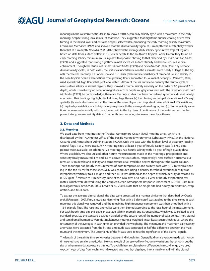
5.1. Impacts on StratificationDiurnal variations in stratification have been shown to affect SST, and hence to be important for air-sea inter-actions in the tropics [e.g. Shinoda, 2005; Kawai and Wada, 2007; Woolnough et al., 2007], so it is useful to con-sider whether daily salinity variations have an appreciable effect on MLD. For the three sites with sufficientsubsurface hourly temperature and salinity data to compute the diurnal MLD cycle, we estimate density andMLD in two ways: (1) using hourly salinity, and (2) using daily-averaged salinity. In both cases, we use hourlytemperatures and compute density and MLD (as defined in section 3), and estimate the diurnal signals ofMLD. At two of the three sites, the daily MLD signal is the same whether computed using hourly or daily salin-ities (Figure 8b and 8c). At 154E,0N in the far western Pacific Ocean, however, the diurnal amplitude of MLDcomputed with the hourly salinity is more than 1.5 times as large as that computed with daily salinity. Evi-dently, the anomalously fresh afternoon conditions (Figure 3b) produce a thinner afternoon mixed layer(Figure 8a). Similarly, the salty morning mixed layer at this site (Figure 3c) produces a much deeper mixed

Figure 7. (a) As for Figure 3a, but showing the amplitude of the daily 1 m temperature signal at the 33 mooring sites where enough hourlywere available to estimate the diurnal signal. (b) Diurnal amplitude of 1 m temperature plotted against diurnal amplitude of 1 m salinity.



layer compared to the daily-average salinity case. The effectof salinity on MLD is asymmetri-cal throughout the day: morn-ing salinity variations produce amixed layer around 1 m thickercompared to the daily-meansalinity case, whereas afternoonsalinity variations cause only a0.5 m MLD difference. Potentialimplications of this finding aredescribed in the discussion sec-tion below. Interestingly, at thenearby 161E,0N site, diurnalsalinity appears to have noimpact on diurnal MLD (Figure8b) despite being only7� longitude from the 154Esite (Figure 8a).

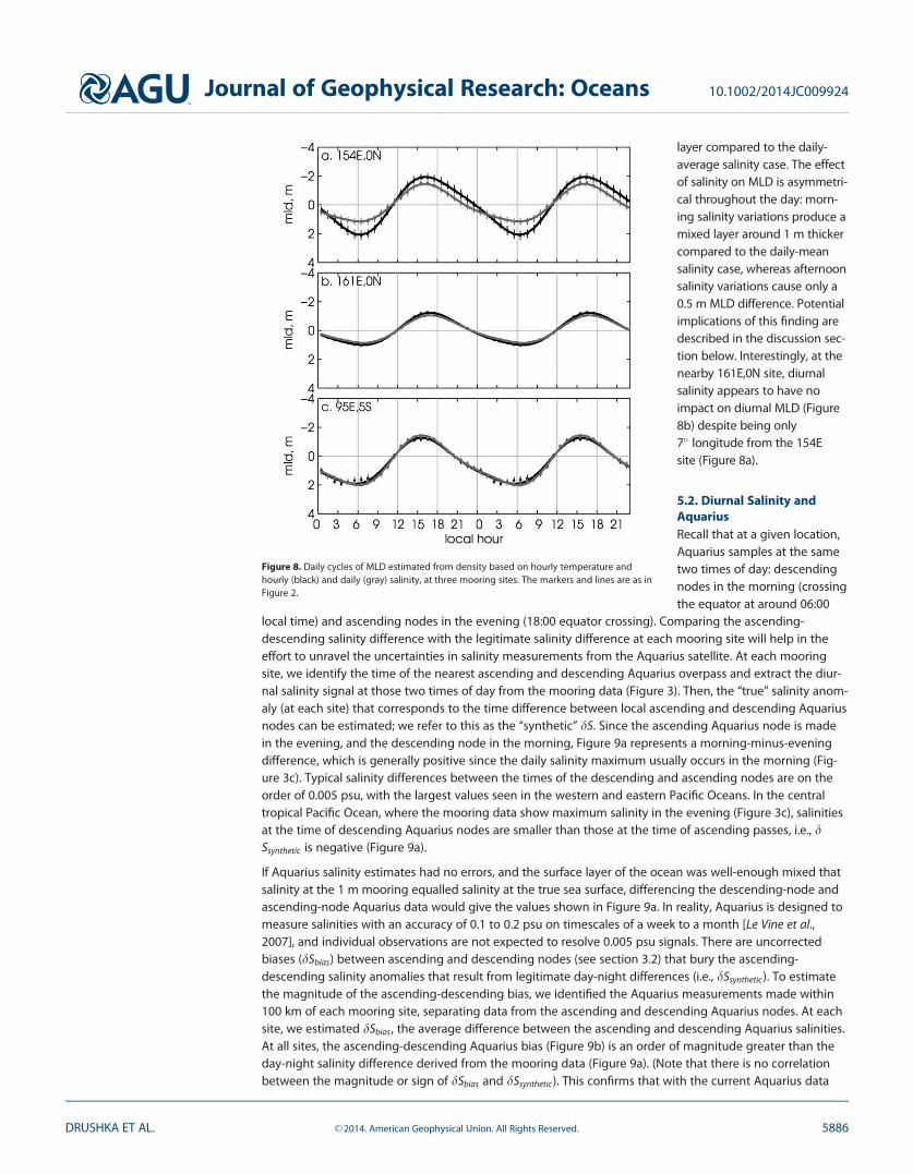
5.2. Diurnal Salinity andAquariusRecall that at a given location,Aquarius samples at the sametwo times of day: descendingnodes in the morning (crossingthe equator at around 06:00

local time) and ascending nodes in the evening (18:00 equator crossing). Comparing the ascending-descending salinity difference with the legitimate salinity difference at each mooring site will help in theeffort to unravel the uncertainties in salinity measurements from the Aquarius satellite. At each mooringsite, we identify the time of the nearest ascending and descending Aquarius overpass and extract the diur-nal salinity signal at those two times of day from the mooring data (Figure 3). Then, the ‘‘true’’ salinity anom-aly (at each site) that corresponds to the time difference between local ascending and descending Aquariusnodes can be estimated; we refer to this as the ‘‘synthetic’’ dS. Since the ascending Aquarius node is madein the evening, and the descending node in the morning, Figure 9a represents a morning-minus-eveningdifference, which is generally positive since the daily salinity maximum usually occurs in the morning (Fig-ure 3c). Typical salinity differences between the times of the descending and ascending nodes are on theorder of 0.005 psu, with the largest values seen in the western and eastern Pacific Oceans. In the centraltropical Pacific Ocean, where the mooring data show maximum salinity in the evening (Figure 3c), salinitiesat the time of descending Aquarius nodes are smaller than those at the time of ascending passes, i.e., dSsynthetic is negative (Figure 9a).

If Aquarius salinity estimates had no errors, and the surface layer of the ocean was well-enough mixed thatsalinity at the 1 m mooring equalled salinity at the true sea surface, differencing the descending-node andascending-node Aquarius data would give the values shown in Figure 9a. In reality, Aquarius is designed tomeasure salinities with an accuracy of 0.1 to 0.2 psu on timescales of a week to a month [Le Vine et al.,2007], and individual observations are not expected to resolve 0.005 psu signals. There are uncorrectedbiases (dSbias) between ascending and descending nodes (see section 3.2) that bury the ascending-descending salinity anomalies that result from legitimate day-night differences (i.e., dSsynthetic). To estimatethe magnitude of the ascending-descending bias, we identified the Aquarius measurements made within100 km of each mooring site, separating data from the ascending and descending Aquarius nodes. At eachsite, we estimated dSbias , the average difference between the ascending and descending Aquarius salinities.At all sites, the ascending-descending Aquarius bias (Figure 9b) is an order of magnitude greater than theday-night salinity difference derived from the mooring data (Figure 9a). (Note that there is no correlationbetween the magnitude or sign of dSbias and dSsynthetic). This confirms that with the current Aquarius data

Figure 8. Daily cycles of MLD estimated from density based on hourly temperature andhourly (black) and daily (gray) salinity, at three mooring sites. The markers and lines are as inFigure 2.



products, simply differencing the ascending and descending Aquarius nodes is not a viable method forextracting day-night salinity differences.

6. Conclusions and Discussion

Hourly observations from 35 moorings have been used to estimate the average daily variability of 1 m salin-ity in the tropics. Consistent with three previous studies [Cronin and McPhaden, 1999; Reverdin et al., 2012](J. E. Anderson and S. C. Riser, submitted manuscript, 2014), we show that the amplitude of the daily salinitycycle just below the sea surface is small: less than 0.01 psu and more typically around 0.005 psu. A closeexamination of dynamics at different sites suggests that entrainment and precipitation appear to drive thediurnal salinity cycle (Figure 5). Although we could only estimate the amplitude of entrainment at threelocations, it contributed significantly to diurnal salinity anomalies there. We hypothesize that entrainment,which results from nighttime convective overturning as the sea surface cools, drives the daily increase ofsalinity (with a small contribution from evaporation) and generally sets the phasing of the signal: increasingsalinity at night with a peak between 00:00 and 09:00 (Figure 3c). Precipitation drives the subsequent fresh-ening; since rainfall can be trapped in thin lenses, the fresh anomalies may not be detected at 1 m depthuntil winds or overturning mixes them below the surface. Horizontal salinity advection, estimated at severalequatorial sites having near-surface velocity data, was found to have a negligible contribution to diurnalsalinity.

While our findings are too speculative to predict the amplitude of diurnal salinity variations, we suggestthat the largest salinity anomalies will be found in regions with large diurnal precipitation and mixed-layerdepth variations and strong salinity stratification. Based on estimates of diurnal precipitation from theTRMM satellite and DS=h from the MIMOC climatology (Figure 6), these regions include the northern Bay ofBengal, the Indonesian Seas, and the eastern equatorial upwelling regions in the Pacific and AtlanticOceans. Diurnal entrainment is challenging to estimate because it requires knowledge of diurnal MLD vari-ability. As a proxy, we computed mean Monin-Obukhov length scales following Schneider and M€uller [1990].Although it gave some insight into patterns of diurnal entrainment, the method is limited to regions havinga net heat flux <37 W m22, which eliminated most areas outside of the equatorial band. Moreover, it is verymuch an approximation, and in situ observations and/or modeling studies are needed in order to moreaccurately quantify diurnal MLD variations throughout the ocean. Argo has previously been used to esti-mate diurnal variations in subsurface temperature [Gille, 2012] and may prove to be a useful tool for quanti-fying diurnal MLD, particularly with the proliferation of floats having high vertical resolution, which moreaccurately resolve subtle variations in MLD.

Quantifying the impacts of precipitation and evaporation on diurnal salinity (Figure 5) relied on the assump-tions that (a) rain-driven anomalies penetrate to 3 m, an estimate based on the size of a freshwater lens esti-mated to arise from observed rain events; and (b) evaporation produces surface salinity anomalies that mixdown to 1 m depth, which was based on stability analysis of a water parcel undergoing typical rates ofevaporation. In fact, rainfall has been shown to drive surface freshening over depths ranging from

Figure 9. (a) Salinity at the time of the local ascending Aquarius pass (around 18:00) minus salinity at the time of the local descendingAquarius pass (around 06:00). Salinities are taken from the fits to 1 m mooring salinities (Figure 3); only sites with statistically significant fitsare plotted. (b) Mean difference between Aquarius descending-node and ascending-node salinities based on Aquarius measurementsmade within 100 km of each mooring site. Note the different color scales in Figures 9a and 9b.



centimeters to more than 10 m [Katsaros and Buettner, 1969; Price, 1979; Wijesekera et al., 1999; Soloviev andLukas, 2006; McCulloch et al., 2012; Reverdin et al., 2012], and the effects of evaporation near the sea surfaceare not well understood [Yu, 2010; Asher et al., 2014a]. Precipitation-related and evaporation-related salinityanomalies are highly dependent on local winds and background stratification [Asher et al., 2014b] and maychange from one day to the next, suggesting that fixed values of hP and hE in equation (2) may be an over-simplification. Understanding the three-dimensional dispersion of salinity anomalies on timescales ofminutes to days is necessary in order to understand the diurnal cycle of surface salinity, and will requireboth modeling and observational efforts.

This study has uncertain conclusions regarding the impacts of diurnal salinity variations on upper oceanstratification. It is an important question, as diurnal variations in MLD appear to modulate SST on intraseaso-nal time scales [Shinoda, 2005]. We have shown that at 154E,0N in the western Pacific warm pool, salinity isresponsible for half of the average daily variation in MLD, which hints at a potentially substantial role ofsalinity in air-sea feedback processes. However, less than 1000 km away at 161E,0N, salinity does not appearto affect diurnal MLD. These results are compelling enough to warrant further investigation of the diurnalsalinity signal in the tropics.

Finally, we consider diurnal salinity variability in the context of the Aquarius satellite salinity mission. Aquarius isin a sun-synchronous orbit, so that ascending and descending nodes cross a given latitude in the evening andthe morning, respectively. For other satellite data sets, this feature has been exploited to extract informationabout day-night differences—for example, in winds [Gille et al., 2003] and SST [Stuart-Menteth et al., 2003]. Wefound that ascending-descending biases in Aquarius data are an order of magnitude greater than the actualday-night salinity anomalies observed at the moorings, indicating that great care must be taken in interpretingday-night differences observed in Aquarius salinities. Our results also have implications if empirical correctionsare applied to the ascending-descending biases in Aquarius salinities: actual day-night salinity anomalies arenonzero at the mooring sites, and likely to be large throughout many regions of the tropics (Figure 6). The pres-ent study used mooring data at 1 m depth, in contrast to the true SSS that Aquarius measures. A recent studyusing Argo floats that profile to within 0.2 m of the surface (J. E. Anderson and S. C. Riser, submitted manu-script, 2014) showed that the diurnal salinity signal at that depth can be about an order of magnitude greaterthan the diurnal salinity signal at 1 m depth, suggesting that diurnal salinity at the sea surface may in fact bestrong enough to be comparable to Aquarius ascending-descending SSS differences. This implies that caremust be taken in correcting the ascending-descending differences in Aquarius, as some of the apparent biascould potentially contain a legitimate diurnal signal. Fully resolving the relationship between true surface salin-ity and near surface (e.g. 1 m depth) will require in situ observations of true SSS over numerous diurnal cyclesin a variety of locations. Extending current observation networks such as the surface drifter program and Argofloats that profile close to the sea surface will be extremely valuable for this task.

ReferencesAnderson, S., R. Weller, and R. Lukas (1996), Surface buoyancy forcing and the mixed layer of the western Pacific warm pool: Observations

and 1D model results, J. Clim., 9(12), 3056–3085.

Asher, W. E., A. T. Jessup, and D. Clark (2014a), Stable near-surface ocean salinity stratifications due to evaporation observed duringSTRASSE, J. Geophys. Res. Oceans, 119, 3219–3233, doi:10.1002/2014JC009808.

Asher, W. E., A. T. Jessup, R. Branch, and D. Clark (2014b), Observations of rain-induced near surface salinity anomalies, J. Geophys. Res.Oceans, doi:10.1002/2014JC009954.

Bernie, D., S. Woolnough, J. Slingo, and E. Guilyardi (2005), Modeling diurnal and intraseasonal variability of the ocean mixed layer, J. Clim.,18(8), 1190–1202.

Bernie, D., E. Guilyardi, G. Madec, J. Slingo, and S. Woolnough (2007), Impact of resolving the diurnal cycle in an ocean-atmosphere GCM.Part 1: A diurnally forced OGCM, Clim. Dyn., 29(6), 575–590, doi:10.1007/s00382-007-0249-6.

Brainerd, K., and M. Gregg (1997), Turbulence and stratification on the tropical ocean-global atmosphere-coupled ocean-atmosphereresponse experiment microstructure pilot cruise, J. Geophys. Res., 102(C5), 10,437–10.

Clayson, C. A., and A. S. Bogdanoff (2013), The effect of diurnal sea surface temperature warming on climatological air-sea fluxes, J. Clim.,26(8), 2546–2556.

Cronin, M. F., and W. S. Kessler (2009), Near-surface shear flow in the tropical Pacific cold tongue front, J. Phys. Oceanogr., 39(5), 1200–1215.

Cronin, M. F., and M. J. McPhaden (1999), Diurnal cycle of rainfall and surface salinity in the western Pacific warm pool, Geophys. Res. Lett.,26(23), 3465–3468.

Cronin, M. F., C. W. Fairall, and M. J. McPhaden (2006), An assessment of buoy-derived and numerical weather prediction surface heatfluxes in the tropical Pacific, J. Geophys. Res. Oceans, 111, C06038, doi:10.1029/2005JC003324.

Danabasoglu, G., W. G. Large, J. J. Tribbia, P. R. Gent, B. P. Briegleb, and J. C. McWilliams (2006), Diurnal coupling in the tropical oceans ofCCSM3, J. Clim., 19(11), 2347–2365.

AcknowledgmentsWe gratefully acknowledge thesources of data for this study: the TAOProject Office of NOAA/PMEL (mooringdata) and NOAA (MIMOC climatology),NASA (Aquarius and TRMM data), theWorld Data Center for Climate(HOAPSv3.2 data), the Indian NationalCentre for Ocean Information Services(TropFlux data). This work wassupported by NASA awardNNX13AO38G (J.S., K.D.) and NOAAgrant NA10OAR4310139 (S.T.G., K.D.).We thank two anonymous reviewersfor their suggestions.



http://dx.doi.org/10.1002/2014JC009808

http://dx.doi.org/10.1002/2014JC009954

http://dx.doi.org/10.1007/s00382-007-0249-6

http://dx.doi.org/10.1029/2005JC003324

de Boyer Mont�egut, C., J. Mignot, A. Lazar, and S. Cravatte (2007), Control of salinity on the mixed layer depth in the world ocean: 1. Generaldescription, J. Geophys. Res, 112, C06011, doi:10.1029/2006JC003953.

Durack, P. J., and S. E. Wijffels (2010), Fifty-year trends in global ocean salinities and their relationship to broad-scale warming, J. Clim.,23(16), 4342–4362.

Fairall, C., E. F. Bradley, J. Hare, A. Grachev, and J. Edson (2003), Bulk parameterization of air-sea fluxes: Updates and verification for theCOARE algorithm, J. Clim., 16(4), 571–591.

Fairall, C. W., E. F. Bradley, D. P. Rogers, J. B. Edson, and G. S. Young (1996), Bulk parameterization of air-sea fluxes for tropical ocean-globalatmosphere coupled-ocean atmosphere response experiment, J. Geophys. Res., 101(C2), 3747–3764.

Fennig, K., A. Andersson, S. Bakan, C.-P. Klepp, and M. Schr€oder (2012), Hamburg Ocean Atmosphere Parameters and Fluxes from SatelliteData—HOAPS 3.2—Monthly Means/6-Hourly Composites, [electronic], Satell. Appl. Fac. on Clim. Monit., doi:10.5676/EUM_SAF_CM/HOAPS/V001.

Gille, S. (2012), Diurnal variability of upper ocean temperatures from microwave satellite measurements and Argo profiles, J. Geophys. Res.,117, C11027, doi:10.1029/2012JC007883.

Gille, S. T., S. G. L. Smith, and S. M. Lee (2003), Measuring the sea breeze from QuikSCAT scatterometry, Geophys. Res. Lett., 30(3), 1114, doi:10.1029/2002GL016230.

Gille, S. T., S. G. L. Smith, and N. M. Statom (2005), Global observations of the land breeze, Geophys. Res. Lett., 32, L05605, doi:10.1029/2004GL022139.

Henocq, C., J. Boutin, G. Reverdin, F. Petitcolin, S. Arnault, and P. Lattes (2010), Vertical variability of near-surface salinity in the tropics: Con-sequences for l-band radiometer calibration and validation, J. Atmos. Oceanic Technol., 27(1), 192–209.

Huffman, G. J., D. T. Bolvin, E. J. Nelkin, D. B. Wolff, R. F. Adler, G. Gu, Y. Hong, K. P. Bowman, and E. F. Stocker (2007), The TRMM Multisatel-lite Precipitation Analysis (TMPA): Quasi-global, multiyear, combined-sensor precipitation estimates at fine scales, J. Hydrometeorol.,8(1), 38–55.

Janowiak, J. E., P. A. Arkin, and M. Morrissey (1994), An examination of the diurnal cycle in oceanic tropical rainfall using satellite and in situdata, Mon. Weather Rev., 122(10), 2296–2311.

Katsaros, K., and K. J. Buettner (1969), Influence of rainfall on temperature and salinity of the ocean surface, J. Appl. Meteorol., 8(1), 15–18.Kawai, Y., and A. Wada (2007), Diurnal sea surface temperature variation and its impact on the atmosphere and ocean: A review, J. Ocean-

ogr., 63(5), 721–744.Kikuchi, K., and B. Wang (2008), Diurnal precipitation regimes in the global tropics, J. Clim., 21(11), 2680–2696.Kumar, P., J. Vialard, M. Lengaigne, V. Murty, and M. McPhaden (2012), Tropflux: Air-sea fluxes for the global tropical oceans-description

and evaluation, Clim. Dyn., 38, 1521–1543.Lagerloef, G., F. Colomb, D. Le Vine, F. Wentz, S. Yueh, C. Ruf, J. Lilly, J. Gunn, and Y. Chao (2008), The Aquarius/SAC-D mission: Designed to

meet the salinity remote-sensing challenge, Oceanography, 21(1), 68–81.Le Vine, D. M., G. S. Lagerloef, F. R. Colomb, S. H. Yueh, and F. A. Pellerano (2007), Aquarius: An instrument to monitor sea surface salinity

from space, IEEE Trans. Geosci. Remote Sens., 45(7), 2040–2050.Li, Y., W. Han, T. Shinoda, C. Wang, R.-C. Lien, J. N. Moum, and J.-W. Wang (2013), Effects of the diurnal cycle in solar radiation on the tropi-

cal Indian Ocean mixed layer variability during wintertime Madden-Julian Oscillations, J. Geophys. Res. Oceans, 118, 4945–4964, doi:10.1002/jgrc.20395.

Lien, R.-C., D. R. Caldwell, M. Gregg, and J. N. Moum (1995), Turbulence variability at the equator in the central Pacific at the beginning ofthe 1991–1993 El Ni~no, J. Geophys. Res., 100(C4), 6881–6898.

Lukas, R., and E. Lindstrom (1991), The mixed layer of the western equatorial Pacific Ocean, J. Geophys. Res., 96(S01), 3343–3357.Maes, C., B. Dewitte, J. Sudre, V. Garcon, and D. Varillon (2013), Small-scale features of temperature and salinity surface fields in the Coral

Sea, J. Geophys. Res. Oceans, 118, 5426–5438, doi:10.1002/jgrc.20344.McCreary, J. P., K. E. Kohler, R. R. Hood, S. Smith, J. Kindle, A. S. Fischer, and R. A. Weller (2001), Influences of diurnal and intraseasonal forc-

ing on mixed-layer and biological variability in the central Arabian Sea, J. Geophys. Res., 106(C4), 7139–7155.McCulloch, M., P. Spurgeon, and A. Chuprin (2012), Have mid-latitude ocean rain-lenses been seen by the SMOS satellite?, Ocean Modell.,

43, 108–111.Miller, J. R. (1976), The salinity effect in a mixed layer ocean model, J. Phys. Oceanogr., 6(1), 29–35.Nesbitt, S. W., and E. J. Zipser (2003), The diurnal cycle of rainfall and convective intensity according to three years of TRMM measure-

ments, J. Clim., 16(10), 1456–1475.Price, J. F. (1979), Observations of a rain-formed mixed layer, J. Phys. Oceanogr., 9(3), 643–649.Reverdin, G., S. Morisset, J. Boutin, and N. Martin (2012), Rain-induced variability of near sea-surface T and S from drifter data, J. Geophys.

Res., 117, C02032, doi:10.1029/2011JC007549.Roemmich, D., and J. Gilson (2009), The 2004–2008 mean and annual cycle of temperature, salinity, and steric height in the global ocean

from the Argo program, Prog. Oceanogr., 82(2), 81–100.Schmidtko, S., G. C. Johnson, and J. M. Lyman (2013), MIMOC: A global monthly isopycnal upper-ocean climatology with mixed layers, J.

Geophys. Res. Oceans, 118, 1658–1672, doi:10.1002/jgrc.20122.Schneider, N., and P. M€uller (1990), The meridional and seasonal structures of the mixed-layer depth and its diurnal amplitude observed

during the Hawaii-to-Tahiti Shuttle experiment, J. Phys. Oceanogr., 20(9), 1395–1404.Shinoda, T. (2005), Impact of the diurnal cycle of solar radiation on intraseasonal SST variability in the western equatorial Pacific, J. Clim.,

18(14), 2628–2636.Soloviev, A., and R. Lukas (1997), Observation of large diurnal warming events in the near-surface layer of the western equatorial pacific

warm pool, Deep Sea Res., Part I, 44(6), 1055–1076.Soloviev, A., and R. Lukas (2006), The near-surface layer of the ocean: Structure, dynamics and applications, chap. 4, in Atmospheric and

Oceanographic Sciences Library, vol. 31, Springer, Dordrecht, Netherlands.Soloviev, A., and N. Vershinsky (1982), The vertical structure of the thin surface layer of the ocean under conditions of low wind speed,

Deep Sea Res., Part A, 29(12), 1437–1449.Sprintall, J., and M. Tomczak (1992), Evidence of the barrier layer in the surface layer of the tropics, J. Geophys. Res., 97(C5), 7305–7316.Stuart-Menteth, A. C., I. S. Robinson, and P. G. Challenor (2003), A global study of diurnal warming using satellite-derived sea surface tem-

perature, J. Geophys. Res., 108(C5), 3155, doi:10.1029/2002JC001534.Tomczak, M. (1995), Salinity variability in the surface layer of the tropical western Pacific Ocean, J. Geophys. Res., 100(C10), 20,499–20,515.Venkatram, A. (1980), Estimating the Monin-Obukhov length in the stable boundary layer for dispersion calculations, Boundary Layer Mete-

orol., 19(4), 481–485.



http://dx.doi.org/10.1029/2006JC003953

http://dx.doi.org/10.5676/EUM_SAF_CM/HOAPS/V001

http://dx.doi.org/10.5676/EUM_SAF_CM/HOAPS/V001

http://dx.doi.org/10.1029/2012JC007883

http://dx.doi.org/10.1029/2002GL016230

http://dx.doi.org/10.1029/2004GL022139

http://dx.doi.org/10.1029/2004GL022139

http://dx.doi.org/10.1002/jgrc.20395


http://dx.doi.org/10.1029/2011JC007549


http://dx.doi.org/10.1029/2002JC001534

Vialard, J., et al. (2009), Cirene: Air-sea interactions in the Seychelles-Chagos Thermocline Ridge region, Bull. Am. Meteorol. Soc., 90(1), 45–61.Wijesekera, H., C. Paulson, and A. Huyer (1999), The effect of rainfall on the surface layer during a westerly wind burst in the western equa-

torial pacific, J. Phys. Oceanogr., 29(4), 612–632.Wijesekera, H. W., and M. C. Gregg (1996), Surface layer response to weak winds, westerly bursts, and rain squalls in the western Pacific

Warm Pool, J. Geophys. Res., 101(C1), 977–997.Woods, J. (1980), Diurnal and seasonal variation of convection in the wind-mixed layer of the ocean, Q. J. R. Meteorol. Soc., 106(449), 379–

394.Woods, J. D., W. Barkmann, and A. Horch (1984), Solar heating of the oceansdiurnal, seasonal and meridional variation, Q. J. R. Meteorol.

Soc., 110(465), 633–656.Woolnough, S., F. Vitart, and M. Balmaseda (2007), The role of the ocean in the Madden-Julian Oscillation: Implications for MJO prediction,

Q. J. R. Meteorol. Soc., 132(622), 117–128.Yu, L. (2010), On sea surface salinity skin effect induced by evaporation and implications for remote sensing of ocean salinity, J. Phys. Oce-

anogr., 40(1), 85–102, doi:10.1175/2009JPO4168.1.Yueh, S. (2013), Aquarius CAP Algorithm and Data User Guide, 2nd ed., Jet Propul. Lab., Pasadena, Calif.



http://dx.doi.org/10.1175/2009JPO4168.1

Documents

PUBLICATIONS - Scripps Institution of Oceanographysgille/pub_dir/jgrc20874.pdf · can indirectly affect SST by modulating upper ocean stratiﬁcation [Lukas and Lindstrom, 1991; de