Embed Size (px)
Citation preview
CHARACTERIZATION OF LANDSCAPE-SCALE HABITAT USE
BY TIMBER RATTLESNAKES (CROTALUS HORRIDUS) WITHIN
THE RIDGE AND VALLEY AND HIGHLANDS REGIONS
OF NEW JERSEY
by
KRIS ALANE SCHANTZ
A thesis submitted to the
Graduate School-New Brunswick
Rutgers, The State University of New Jersey
in partial fulfillment of the requirements
for the degree of
Master of Science
Graduate Program in Ecology and Evolution
written under the direction of
Dr. Joanna Burger
and approved by
_____________________________________
_____________________________________
_____________________________________
New Brunswick, New Jersey May 2009

ii
ABSTRACT OF THE THESIS
Characterization of Landscape-scale Habitat Use by Timber Rattlesnakes
(Crotalus horridus) within the Ridge and Valley and Highlands Regions of
New Jersey
By KRIS ALANE SCHANTZ
THESIS DIRECTOR:
DR. JOANNA BURGER
Regulations and a lack of understanding the habitat needs of timber rattlesnakes
(Crotalus horridus) on a landscape-scale have limited conservation efforts. With better
information land managers and planners could implement strategies that protect suitable
habitats from development and other human activities. While studies have shown
microhabitat characteristics play a role in habitat selection by timber rattlesnakes, it
remains unclear if large-scale features, other than rock outcrops, talus slopes and canopy,
also impact site selection. I compared the habitat use by two metapopulations of timber
rattlesnakes in northern New Jersey with available habitats using GIS data layers to
identify the snakes’ macrohabitat preferences. The results showed snakes used habitats
with slightly more open canopy, closer to rock outcrops, and farther from roads, human
development, forest edge (an interface between any habitat and forests with >50%
canopy closure) and streams and rivers (>10m wide) than randomly sampled locations.
Additionally, I developed a model and distribution map of potential areas where
hibernacula may exist in northern New Jersey by first testing habitat and topographic

iii
variables to determine the predictors of suitable habitat for hibernacula. In 2004,
elevation, sun index, deciduous wetlands and slopes (0-20%) were the most influential
features in predicting suitable habitat for hibernacula. Slopes (0-20%) and deciduous
wetlands were negatively associated with hibernacula indicating that areas containing
shallow slopes and/or deciduous wetlands were less likely to support hibernacula. Sun
index indicated that hibernacula are most likely to be found in areas with steep slopes and
southerly aspects, and elevation, having the least influence in predicting suitable habitat
for hibernacula, showed the likelihood of hibernacula presence increased with increasing
elevation. In 2009, with the addition of interior forest hibernacula in the dataset, only
slope (0-20%) and sun index were influential features in predicting suitable habitat for
hibernacula indicating that the potential for hibernacula presence increased in areas with
steep slopes and southerly aspects. Landscape modeling using GIS-ready habitat features
can help biologists identify habitats essential for populations and metapopulations, and
target conservation of those habitats and connecting corridors for long-term timber
rattlesnake viability.

iv
ACKNOWLEDGEMENTS
This research was funded by the National Park Service (1999-2000) and the US Fish
and Wildlife Service, State Wildlife Grants (2003-2009). I give special thanks to
Gretchen Fowles, NJ Division of Fish and Wildlife, Endangered and Nongame Species
Program (ENSP), for her patience and generosity during the development and refinement
of the hibernacula model and preparation of the foraging model. Without her assistance
and GIS-related guidance, this paper would not exist. I also thank Sharon Petzinger,
ENSP, for providing assistance with statistical analyses. Special thanks to MacKenzie
Hall, Conserve Wildlife Foundation of NJ, formerly “Observer 2” (in Chapter 3’s
discussion) of ENSP, for her tireless and devoted field assistance to the ENSP and to the
rattlesnakes. I thank David Jenkins, Bureau Chief, ENSP, for his patience and guidance
in focusing my objectives; Kathleen Clark, Supervising Biologist, ENSP, for her constant
encouragement and guidance; Michael Valent, Principal Zoologist, ENSP, for his support
and guidance over the many years we’ve worked together and for introducing me to
rattlesnakes.
Also, I am extremely grateful to my brother, Erik, for his understanding, support and
advice over my lifetime. Special thanks to Kathleen Michell and George Banta for the
many educational field days, collaboration on projects and for being supportive of all my
endeavors, and specifically Kathleen for sharing her expertise and knowledge of timber
rattlesnakes. Special thanks to the ENSP staff that assisted in data collection, which
enabled me to fulfill other responsibilities. I’d like to also thank Dr. Howard Reinert,
who over the years has provided me with invaluable information and understanding of

v
rattlesnake behavior and to W.H. (Marty) Martin and Michael Marchand for sharing their
expertise.
Special thanks to Marsha Morin, graduate program administrator for the Ecology
and Evolution Graduate Program at Rutgers University. Marsha has never ceased to
amaze me with her kindness and patience in guiding a part-time student through the maze
of graduate school requirements. I believe without her, graduate school would have been
much more difficult to navigate. Finally, I’d like to thank my Advisory Committee, Drs.
Joanna Burger, Richard Lathrop and Edwin Green for their guidance and assistance
during the course of this research. I also thank them for their patience and understanding,
their encouragement to finish what I started and the kindnesses they’ve shown me over
the years.

vi
TABLE OF CONTENTS
ABSTRACT OF THE THESIS .......................................................................................... ii ACKNOWLEDGEMENTS............................................................................................... iv TABLE OF CONTENTS................................................................................................... vi LIST OF TABLES............................................................................................................. ix LIST OF ILLUSTRATIONS............................................................................................. xi CHAPTER 1: INTRODUCTION....................................................................................... 1
Study Species:.................................................................................................................. 3 Objectives: ....................................................................................................................... 5 Background: .................................................................................................................... 6
Research...................................................................................................... 6 Habitat Modeling and Conservation ........................................................... 9
CHAPTER 2: MODEL DEPICTING SUITABLE HABITAT FOR TIMBER RATTLESNAKE HIBERNACULA ................................................................ 16
MATERIALS AND METHODS: ........................................................................... 17
Study Area........................................................................................................ 17 Data Collection and Compilation..................................................................... 18
Model Preparation..................................................................................... 18
Field Reconnaissance................................................................................ 22
Model Development......................................................................................... 23
RESULTS: .............................................................................................................. 25 DISCUSSION: ........................................................................................................ 29
Model Suitability.............................................................................................. 29
vii
Implications for Management of Rattlesnakes................................................. 33 CHAPTER 3: IDENTIFYING LANDSCAPE-SCALE FEATURES AND PARAMETERS OF SUMMER RANGE......................................................................... 35
MATERIALS AND METHODS: ........................................................................... 36
Study Area........................................................................................................ 36 Radio-telemetry................................................................................................ 38
Transmitters .............................................................................................. 38 Snake Capture and Implantation............................................................... 40 Tracking .................................................................................................... 43
Generating Random Sampling Points .............................................................. 45
Microhabitat.............................................................................................. 45 Macrohabitat ............................................................................................. 46
Data Collection ................................................................................................ 46
Snake Locations and Microhabitat............................................................ 48 Random Locations and Microhabitat........................................................ 52 Snake Locations and Macrohabitat........................................................... 53 Random Locations and Macrohabitat ....................................................... 54
Analysis............................................................................................................ 54
Micro- and Macrohabitat .......................................................................... 55
RESULTS: .............................................................................................................. 58
Tracking Successes and Failures...................................................................... 58 Microhabitat Analysis ...................................................................................... 58 Microhabitat Dataset ........................................................................................ 61 Macrohabitat Analysis ..................................................................................... 63

viii
Macrohabitat Dataset ....................................................................................... 69
DISCUSSION: ........................................................................................................ 71
Micro- and Macrohabitat Play a Role in Site Selection................................... 71 Potential Biases in Data Collection.................................................................. 78 Future Research................................................................................................ 80 Future Applications.......................................................................................... 83
TABLES ........................................................................................................................... 85 ILLUSTRATIONS ......................................................................................................... 111 APPENDICES ................................................................................................................ 116 LITERATURE CITED ................................................................................................... 178

ix
LIST OF TABLES Table 1: Potential habitat predictors of hibernacula and their resultant significance... .... 85 Table 2a: Final habitat selection model depicting suitable habitat for hibernacula, 2004................................................................................................................................... 88 Table 2b: Final habitat selection model depicting suitable habitat for hibernacula, 2009................................................................................................................................... 88 Table 3: Landscape-scale features tested for significance at snake-used versus available habitat within and between study sites.............................................................................. 89 Table 4: Categorical ranges of measures for large-scale features generated by using snake location data and scatter plots................................................................................. 90 Table 5: Data subsets used to compare snake-used and available habitats at and between study sites. .......................................................................................................... 91 Table 6: Random sample points excluded from the Highlands Region data collection. .. 92 Table 7a: Statistical results; snake-used versus available microhabitats within the Kittatinny Ridge study site................................................................................................ 93 Table 7b: Statistical results; snake-used versus available microhabitats within the Highlands Region study site. ............................................................................................ 94 Table 7c: Statistical results; snake-used microhabitats of the Kitattinny Ridge versus Highlands Region study sites............................................................................................ 95 Table 7d: Statistical results; comparing available microhabitats of the Kitattinny Ridge versus Highlands Region study sites................................................................................. 96 Table 7e: Statistical results; snake-used microhabitats of both study sites (Kitattinny Ridge and Highlands Region) versus the available microhabitats of both study sites. .... 97 Table 8a: Statistical results; snake-used versus available habitats with regard to landscape-scale features within the Kittatinny Ridge study site....................................... 98 Table 8b: Statistical results; snake-used versus available habitats with regard to landscape-scale features within the Highlands Region..................................................... 99 Table 8c: Statistical results; snake-used habitats with regard to landscape-scale features within the Kitattinny Ridge versus Highlands Region study sites.................................. 100

x
Table 8d: Statistical results; comparing available habitats with regard to landscape- scale features within the Kitattinny Ridge versus Highlands Region study sites. .......... 101 Table 8e: Statistical results; comparing snake-used habitats of both study sites (Kitattinny Ridge and Highlands Region) versus the available habitats of both study sites with regard to landscape-scale features. ................................................................. 102 Table 8f: Statistical results; snake-used versus available habitats within the Kittatinny Ridge study site for canopy closure. ............................................................................... 103 Table 8g: Statistical results; snake-used versus available habitats within the Highlands Region for canopy closure. ............................................................................................. 104 Table 8h: Statistical results; comparing snake-used habitats within the Kittatinny Ridge versus the Highlands Region study sites for canopy closure. .............................. 105 Table 8i: Statistical results; comparing available habitats within the Kittatinny Ridge versus the Highlands Region study sites for canopy closure.......................................... 106 Table 8j: Statistical results; comparing snake-used habitats of both study sites (Kitattinny Ridge and Highlands Region) versus the available habitats of both study sites for canopy closure................................................................................................... 106 Table 8k: Statistical results; snake-used versus available habitats within the Highlands Region regarding proximity to nearest rock outcrop............................... 107 Table 9a: Mean percentages of snake and random locations' canopy closure for the majority of the study samples. ........................................................................................ 108 Table 9b: Mean distances of snake and random locations' proximities to streams and rivers for the majority of the study samples.................................................................... 108 Table 9c: Mean distances of snake and random locations' proximities to human- occupied areas for the majority of the study samples. .................................................... 109 Table 9d: Mean distances of snake and random locations' proximities to paved roads for the majority of the study samples.............................................................................. 109 Table 9e: Mean distances of snake and random locations' proximities to the forest edge for the majority of the study samples. .................................................................... 110 Table 9f: Mean distances of snake and random locations' proximities to the nearest rock outcrop (within 50m, Highlands Region study site only) for the majority of the study samples. ................................................................................................................. 110
xi
LIST OF ILLUSTRATIONS
Figure 1: Study area within northern New Jersey........................................................... 111 Figure 2: Classification error rates (% locations correctly classified as used or unused) for rattlesnake hibernacula model, 2009 ........................................................... 112 Figure 3: Map distinguishing suitable versus unsuitable habitat for hibernacula, 2004. 113 Figure 4: Map distinguishing suitable versus unsuitable habitat for hibernacula, 2009. 114 Figure 5: Example of computer-generated random points throughout a study site, ignoring hibernacula buffer overlap, for landscape-scale feature characterization of study sites........................................................................................................................ 115

1
CHAPTER 1: INTRODUCTION
Habitat loss continues to be a major factor affecting long-term viability of both
native flora and fauna. However, habitat fragmentation is an issue widely accepted in the
field of conservation as one of the most detrimental factors impacting our native species
(Bennett 1998, 2003, Gibbons et al. 2000). While natural fragmentation does occur, it is
often the human-induced division of larger habitat patches into smaller areas that
negatively impacts species (Hilty 2006). This could be as obvious as a road bisecting
grasslands or as subtle as improper silviculture practices dividing old growth forests with
younger stands that may not be suitable for all wildlife (Bennett 1998, 2003).
Roads and development that fragment habitats create passage barriers for wildlife,
especially terrestrial-bound species, decreasing their chances of successfully moving
from one habitat patch to another. For smaller, slower-moving species such as reptiles
and amphibians, a road could be impossible to cross safely. These manmade boundaries
often isolate populations, limiting genetic exchange, and in some cases, populations
dwindle until they finally disappear (Bennett 1998, 2003, Parent and Weatherhead 2000).
Additionally, linear edge increases as a habitat patch is divided into multiple smaller
patches. This in turn, increases the edge effect caused when an area extending from the
edge inward is impacted by the events occurring on the exterior of the patch (e.g., traffic,
noise, light, increased number of scavengers or predators) (Bennett 1998, 2003).
Depending on the size of the patch, the entire area could be affected, negatively
impacting the species inhabiting the patch by decreasing their foraging or nesting
success, increasing their stress and stress-induced illnesses (i.e., compromising their

2
immune system) and, for water-dependent species, polluting the waters through
petroleum run-off from roads or fertilizers from managed lawns.
Although a relatively recent primary goal in conservation is to protect or restore
connective corridors between suitable habitats, data gaps remain regarding the
requirements of many species (Hilty 2006). Regardless, conservationists agree that
efforts must be made to decrease fragmentation and maintain or increase connectivity
between populations while continuing to research the habitat requirements of wildlife
species in order to refine and/or improve management strategies (Hilty 2006). In
addition, researchers must continue to locate critical core habitats in need of connective
corridors and target immediate conservation and management efforts to maintain or
enhance resident populations, especially for rare flora and fauna.
For a species such as the timber rattlesnake (Crotalus horridus), conservation
strategies that focus on protecting critical core habitats and travel corridors, while
maintaining connectivity to additional populations, can help improve the status of their
populations through the northeastern United States. These snakes move from their
hibernacula to their foraging grounds, generally the same area each year once they have
established their ranges (although slight annual shifting occurs; Reinert and Zappalorti
1988), with males dispersing during the breeding season in search of females. By
determining habitat parameters at both the microhabitat level and landscape-scale (also
referred to as macrohabitat), habitat management and land-use decisions could be
implemented that protect the needs of this species.
3
Study Species:
The timber rattlesnake (Crotalus horridus) is a thick-bodied, slow moving snake that
relies heavily on its camouflage for self-defense. Timber rattlesnakes are only found in
the eastern half of the United States with its range extending from the northeast to the
southeast and on to the mid-west (Galligan and Dunson 1979, Martin 1992b). Declines
in northeastern timber rattlesnakes’ populations have led to the species being listed as
either extirpated, endangered or threatened in all but three of the Northeast states with
only one population remaining in New Hampshire and two in Vermont (Michael
Marchand, New Hampshire Fish and Game Department, pers. comm.). Most of
Massachusetts’ population has disappeared (Martin 2002) and the Maine and Rhode
Island populations are already considered extirpated (Breisch 1992). New York
considers the species threatened, while New Jersey, Connecticut and Maryland list them
as endangered. Pennsylvania currently has listed timber rattlesnakes as a species of
special concern. The timber rattlesnake (Crotalus horridus, formerly Crotalus horridus
horridus, thus excluding the canebrake rattlesnake) of the northern range of Virginia only
has regulatory protection with regard to commercial trade and transport, up to five may
be held in captivity. West Virginia offers no protection at any level. Delaware’s
population is considered extirpated although there are no substantiated historic records of
their existence.
The rattlesnakes’ life history strategy predisposes them to population declines.
Although timber rattlesnakes are generally long lived, some reaching thirty years of age
(Ernst and Barbour 1989), they have relatively late reproductive maturity. The average
female first reproduces at seven to nine years of age (Martin 1993), requiring females to

4
survive natural and anthropogenic predation and other disturbances over many years
before producing a single litter. Females reproduce every three to four years if they have
had successful forages and experience appropriate weather conditions and temperatures
during gestation (Martin 1993). A typical litter consists of only six to ten young (Ernst
and Barbour 1989) and it is unknown how many young survive their first two winters.
There are reports indicating that only 55 – 68% of yearlings survive their first year
(William H. Martin, pers. comm.).
Additionally, timber rattlesnakes have had a long history of abuse and wanton
killings by humans, even the destruction of entire populations (Galligan and Dunson
1979, Furman 2007). As recently as the early 1970’s, bounties were still awarded for
dead rattlesnakes in New York and Vermont (Furman 2007). As late as the 1960’s,
rattlesnakes were collected from New Jersey’s hibernacula and gestating sites for sale to
local zoos, the pet trade and to laboratories for the production of antivenin and simply to
kill them. With protection from the New Jersey Endangered and Nongame Species
Conservation Act (ENSCA, N.J.S.A. 23:2A-1 to –20) to prevent/minimize illegal
collections and mass killings, the most difficult battles in conservation for this rare and
unique species in New Jersey are preventing citizens from committing wanton killings
and the lack of regulations to protect their critical upland habitats.
As a result of their late reproductive maturity, low fecundity, long intervals between
breeding and the lack of habitat protection, in conjunction with human encounters, long-
term survival of timber rattlesnake populations remains in jeopardy in New Jersey.
Conservation measures to protect the populations must take into account the need to
educate society about the important roles of rattlesnakes in our natural world in an effort

5
to prevent or at least minimize wanton killings. Additional measures include the creation
and acceptance of regulations that protect upland habitats where rattlesnakes have been
documented.
Objectives:
This study uses data gathered from 28 radio-tracked timber rattlesnakes in the
deciduous forests of northern New Jersey to identify landscape-scale features of summer
ranges that could be used to develop a predictive model of suitable summer range
habitats. While habitats identified through the landscape-scale parameters used in this
research may not appear to be “preferred” or “optimum” habitat, the study examines
habitat actually used by the snakes. Once habitat is identified as suitable foraging areas
and/or potential summer range, management strategies can be developed to enhance or
restore lands to optimal conditions that also may suit other rare wildlife (e.g., interior
forest species such as barred owls, Strix varia, red-shouldered hawks, Buteo lineatus, and
bobcats, Lynx rufus). This study also develops a predictive model of suitable habitat for
timber rattlesnake hibernacula. By identifying potential areas where hibernacula exist,
targeted field reconnaissance could result in newly discovered hibernacula for which
management and land-use strategies can be developed to enhance and protect these
critical areas. Additionally, it is equally important to identify and protect core foraging
areas (and the associated travel corridors) associated with known or newly discovered
hibernacula in order for local populations of rattlesnakes to persist.

6
Background: Research
There is much literature describing the natural history (Klauber 1956, Galligan and
Dunson 1979, Martin 1992b), seasonal cycles, home range (Reinert and Zappalorti 1988,
Brown 1992, Martin 1992a) and microhabitat use (Klauber 1956, Reinert 1984a and
1984b, Reinert and Zappalorti 1988) of the timber rattlesnake (Crotalus horridus). Over
the past three to four decades the use of radio-telemetry has provided scientists with
detailed insight into the movements and behavior of this secretive creature that is
otherwise difficult to detect because it is cryptically colored and often sits quiet and still.
Information from these studies has proven invaluable in helping scientists and
conservationists understand the microhabitat requirements of this species. Use of this
knowledge has resulted in the implementation of conservation efforts in most of the
northeastern states through public outreach, the protection of dens and state listings
affording the rattlesnakes protection under state Endangered Species Acts. However, this
species is still considered rare and, regionally, populations remain in jeopardy (Galligan
and Dunson 1979, Breisch 1992, Martin 2002, Michael Marchand, New Hampshire Fish
and Game Department, pers. comm.). More action will need to be taken to protect them
before they are regionally extirpated from the Northeast, including gaining a better
understanding of this snake’s needs on a landscape-scale in relationship to their selected
habitats. Determining the proximity of these sites to human activity may better enable
planners and land managers to manage lands suitable for this rare species and minimize
human-rattlesnake interaction (Peterson 1990, Brown 1993, Parent and Weatherhead
2000).

7
Earlier research has provided information on seasonal movements and behavior,
including individual snake’s core and critical habitats (i.e., foraging areas, dens, gestation
and shed sites, transient areas) over a large area. Rattlesnake activity often centers
around their hibernacula and gestation sites (Martin 1993), with snakes moving around a
“general summer range” during the foraging and breeding season and returning to the
same hibernaculum each fall (Landreth 1973, Reinert and Zappalorti 1988). A study of
eighteen resident rattlesnakes tracked by radio-telemetry (fifteen over one active season
and three over two active seasons) showed that each year, resident snakes used the same
path of egress from the hibernaculum and general activity range (Reinert and Rupert
1999). An earlier study that tracked rattlesnakes over one active season found that
rattlesnakes used the same path of egress from the hibernaculum due to the topography
(Bushar et al. 1988), a finding also supported by Brown et al. (1982) and later by the NJ
Division of Fish and Wildlife, Endangered and Nongame Species Program (ENSP),
unpubl. data (1999 - 2000). These studies support the theory that the landscape plays a
vital role in habitat selection and movement patterns because landscape features influence
the path of an individual’s movements.
In addition to landscape features guiding directional movements to and from the
hibernacula, features can also create barriers that may force snakes to use restricted
corridors between preferred habitat patches (Wiegand et al. 1999). These corridors are
not necessarily preferred habitat (Wiegand et al. 1999), but are critical because they allow
movement through potentially unfavorable areas and connect prime habitat patches
(Anderson and Danielson 1997; Wiegand et al. 1999). These corridors also permit

8
genetic exchange between populations, which may be a crucial factor in maintaining
healthy populations (Kienast 1993; Bushar et al. 1998).
Although there may be a number of preferred habitat patches, without corridors to
reach these areas, they provide little support to the snakes, especially when separated by
heavily traveled roads. In addition, this “landscape-guided” directional path of egress
may affect the population’s overall distribution, their abundance in a given area and
possibly their overall success (Flather and Sauer 1996). For example, the rattlesnakes’
path of travel may influence their choice of habitat use and therefore, the availability of
prey, which, in turn can determine their long-term success. Bushar et al. (1998)
suggested that male dispersal distances should be far enough to encounter females from
other dens to increase genetic exchange and that the encounter rate is influenced by rock
outcrop locations and access to the outcrops. This concept also supports the importance
of landscape structure in habitat selection and the importance of habitat selection on
reproductive success.
Habitat analysis on a landscape level may allow the identification of necessary
corridors, or conversely, the lack of corridors, in addition to critical habitat patches
throughout an area. By identifying and determining the importance of the corridors
(those potentially connecting highly used habitat patches or preferred habitats) and
identifying highly used or preferred habitats, land managers, conservation agencies,
regulators and conservationists can develop conservation strategies to protect these vital
pathways and minimize human activity. Further, with access to Geographic Information
Systems (GIS) and satellite imagery since the early 1980s, scientists have been
developing wildlife habitat mapping for targeting reconnaissance work, guiding habitat
9
management and evaluating habitat suitability (Aspinall and Veitch 1993, Pereira and
Itami 1991, Roseberry et al. 1995 and Rittenhouse et al. 2007).
Habitat Modeling and Conservation
In the 1990’s, Alvin Breisch, New York State Department of Environmental
Conservation, developed a model and habitat suitability map of timber rattlesnake
hibernacula for use in New York state (Alvin Breisch, pers. comm.). The resultant map
was broad in scope and identified many areas as suitable habitat. Breisch expressed that
the difficulty was not in a lack of knowledge about rattlesnake habitat requirements, but
rather the quality of the GIS data layers at that time (Alvin Breisch, pers. comm.).
Browning et al. (2005) also developed a model and probability map to depict suitable
habitat for hibernacula within a Wildlife Management Area of predominantly oak-
hickory and oak-pine forests in northeastern Arkansas. Although confident the model
could assist in targeting reconnaissance efforts, they found the areas identified for
potential hibernacula varied widely in their suitability according to the analysis with
some areas being valued as having a lower probability of presence than others. Browning
et al. (2005) suggested the possibility that more refined GIS data layers (i.e., soil
properties) might help in future modeling of rattlesnake hibernacula.
While Breisch’s model of suitable habitat for hibernacula had the potential to
provide useful information and helped focus this present study’s efforts to create a similar
model, it is unclear if his model has been revisited with more current GIS data layers.
Browning’s study incorporated thirty-nine hibernacula, thirty-five that appeared to have
the standard or typical characteristics as described by Klauber (1956) and Galligan and
10
Dunson (1979), including sun-exposed slopes of talus and ridgeline with southeast to
southwest aspects. Four hibernacula had slightly varying features including two facing
north and northeast and two on steeper slopes (Browning et al. 2005). However, with the
assistance of radio-telemetry, researchers have discovered “atypical” hibernacula within
the interior forest (Howard Reinert, pers. comm., Kathleen Michell, pers. comm.,), some
as much as 100m from the nearest basking area (Kathleen Michell, pers. comm., K.A.
Schantz, pers. obs.). “Interior forest” hibernacula may be critical to each local population
due to the difficulty people have in identifying them, thus decreasing the likelihood of
intentional anthropogenic disturbances at these locations. It does not appear that the
model developed by Brown et al. (2005) used interior forest hibernacula, and it is unclear
if Breisch’s model included similar sites or rather focused on hibernacula satisfying the
standard descriptions (Klauber 1956, Galligan and Dunson 1979). Given the limitations
of GIS, it is possible interior forest hibernacula, at least those found in New Jersey, will
not easily be modeled as they are located under the canopy and at lower elevations than
the more typical talus and ridge-based hibernacula, limiting the characteristics
discernable through GIS. It may be necessary to use surficial and subsurface data
depicted in GIS-ready data layers as they become available. Additionally, a dataset
consisting of mostly “typical” hibernacula with fewer interior forest hibernacula may
skew the analyses of habitat and topographic features that act as predictors of hibernacula
presence, decreasing a model’s ability to identify potential habitats where interior forest
hibernacula exist.
Rittenhouse et al. (2007) developed a habitat suitability index model (HSI; HSIs also
described in Dijak et al. 2007) to identify the suitable habitat (active season) of timber

11
rattlesnakes in the central hardwoods of the Midwestern United States. They used five
variables to value the landscape, including proximity to hibernacula (or hibernacula areas
which usually contain multiple den pockets), early successional foraging habitat, distance
to roads, woody debris (for shelter and foraging) and the proportion of woody debris to
foraging habitat determined by canopy cover. The amount and composition of woody
debris was assumed to be correlated to the age of the forest stand with older stands of
trees (>100 years) containing more woody debris suitable for rattlesnake foraging and a
declining suitability as a stand age decreased. Distance to roads was used as a value of
unsuitable habitat with suitability decreasing as distance to roads decreased.
It would be time-intensive and costly to develop broad-scale field documentation
confirming the presence of woody debris over a large area. Thus, it is understandable
why Rittenhouse et al. (2007) derived a value for woody debris based on stand age.
However, while northern New Jersey’s forests, the focal area of this study, are not
homogeneous, there are few uneven-aged forest stands on public lands where rattlesnakes
are found. This is due, in large part, to the lack of timber harvesting and timber stand
improvement work being conducted on public lands in New Jersey. The National Park
Service does not allow any timber harvests nor do they conduct any timber stand
improvement work on the Delaware Water Gap National Recreation Area (located along
the Kittatinny Ridge, a portion of the Ridge and Valley Region). The NJ Division of
Parks and Forestry conducts very limited timber harvesting or timber stand improvement
work on state-owned forests. Given that many of New Jersey’s forests on public lands
contain older stands rather than uneven-aged forest stands, it would be difficult to
develop a gradient representing the amount of woody debris based on the stand age.

12
Therefore, using a value for woody debris derived from stand age may not be as
successful a predictor in all states, specifically New Jersey, as it was in the study by
Rittenhouse et al. (2007).
Since dispersal distances of rattlesnakes from their hibernacula have been well
documented (Brown 1993), applying the proximity of known hibernacula as a means of
identifying suitable habitat will benefit any model. However, it will only assist in areas
where documented hibernacula exist and will not provide information regarding potential
suitable habitats where snakes have not been observed but may persist.
Additionally, roads themselves are unsuitable for rattlesnakes as the snakes are
exposed to predators and at risk of road mortality (Bonnet et al. 1999, Andrews and
Gibbons 2005, Andrews et al. 2006). Timber rattlesnakes, in particular, may be at greater
risk than other snakes as Andrews and Gibbons (2005) found that while most mature
timber rattlesnakes avoided roads, those that approached or attempted to cross, became
immobilized 50% of the time as vehicles approached and passed. This makes them very
susceptible to both accidental and purposeful road mortality. However, it is unclear if all
habitats near or adjacent to roads are also unsuitable or perhaps suitable but avoided by
snakes due to road influences affecting their ability to detect prey and predators such as
noise pollution, light pollution and increased vibrations (Tuxbury and Salmon 2005,
Andrews and Gibbons 2005, Andrews et al. 2006). While Rittenhouse et al. (2007) found
the snakes avoided areas near roads, I will further examine this feature as roads are of
particular concern for wildlife in New Jersey because of the dense infrastructure within
the State.

13
As urban sprawl continues to pepper New Jersey’s landscape, natural resources and
wildlife will benefit from informed land managers and planners that better understand life
history requirements and how to protect these resources on a larger scale. Timber
rattlesnakes, a state endangered species in New Jersey, are protected under the NJ
Endangered and Nongame Species Conservation Act (ENSCA, N.J.S.A. 23:2A-1 to -20).
However at this time, the act does not explicitly guarantee wildlife the protection of
suitable habitat, but rather only protects individuals. Land-use decisions that consider the
requirements of the rare and endangered snake may assist in the recovery of the timber
rattlesnake in northern New Jersey and perhaps other mountainous northeastern habitats.
It is the responsibility of the state wildlife agency in New Jersey to provide the necessary
information on the distribution and critical habitats of rare wildlife so that planners and
regulators can apply this information when making land-use decisions. As such, the NJ
Division of Fish and Wildlife, Endangered and Nongame Species Program (ENSP)
developed a regulatory map, The Landscape Project (Niles et al. 2001), first released in
2001 and now in Version 2.1, to accomplish this task.
The ENSP continues to revise and refine The Landscape Project maps based on
continuing research and literature reviews. The habitat suitability index model developed
by Rittenhouse et al. (2007) is very similar to The Landscape Project in that they both
identify suitable habitat based on documented preferred habitats and requirements of the
species. The Landscape Project map, however, is also based on confirmed observations
of rare wildlife and builds upon those observations (Niles et al. 2001, Winkler et al.
2008).

14
Additionally, the passing of the Highlands Water Protection and Planning Act in
2004 led the Highlands Council to develop a regional master plan to identify areas within
its region in New Jersey for development and conservation (New Jersey Highlands
Council 2008). The ENSP, in an effort to assist the Highlands Council, created a more
specific species-based patch mapping system to value critical habitat within the
Highlands Region (The Landscape Project, Version 3.0, Highlands; Winkler et al. 2008).
By using a species-based patch system, planners and land managers are able to identify
habitat parcels critical to rattlesnake persistence at a more precise scale than the former
version. The ENSP is working to revise the map for the remainder of the State, but
currently uses Version 2.1 outside of the Highlands Region. The Landscape Project map
and documentation can be found on the Internet at
www.njfishandwildlife.com/ensp/landscape/index.htm.
As a regulatory tool, The Landscape Project critical habitat mapping was created
using documented sightings and minimal extrapolation to habitat typing, and therefore, it
can only provide assistance to land stewards, managers and planners in areas where the
State has documented, confirmed occurrences. Given the cryptic nature of rattlesnakes
and the potential continued decline of populations, a lack of observations does not
necessarily mean an absence of snakes (Kéry 2002). An example of this is a
hibernaculum discovered during ENSP’s research along the Kittatinny Ridge (1999-
2000). After approximately twelve visits to and surveys of the area during the fall
seasons of 1999 and 2000, and the spring of 2000, the hibernaculum was believed to
contain a satellite or depleted population as only a single study snake had been observed
in the area. During the spring, 2001, a revisit to collect the snake for transmitter removal

15
and a brief survey of the neighboring talus revealed seven additional rattlesnakes and two
northern copperheads (Agkistrodon contortrix mokasen). Clearly, this supports the need
to protect and manage habitats that fall within the rattlesnakes’ distribution and are
suitable to sustain them, regardless of whether or not there are reported observations.
However, because The Landscape Project includes a regulatory map based on valuing
potential suitable habitat determined by the ENSP and selected from the habitats
described by the NJ Department of Environmental Protection’s 2002 Level III Land
Use/Land Cover data layer (LU/LC02) with modified descriptions from Anderson
(1976), identification of potential “suitable” habitat would value much of the northern
region of New Jersey if observations were not used as a basis for the valuation. Given
the difficulty to detect the snakes, the timber rattlesnake population recovery and
stabilization may depend on the development and implementation of habitat management
strategies that benefit timber rattlesnakes in suitable areas regardless of whether or not an
observation has been documented. By identifying areas of suitable habitat within the
rattlesnakes’ distribution in northern New Jersey, land managers and planners could
implement management strategies to assist in their recovery.
This research focuses on two components that will assist in the conservation of
timber rattlesnakes (Crotalus horridus) in northern New Jersey. The first, described in
Chapter 2, is to develop a model that depicts suitable habitat for hibernacula. The
second, described in Chapter 3, is to identify landscape-scale features and parameters that
will be used to develop a future model depicting suitable habitat for the snakes’ summer
range.

16
CHAPTER 2: MODEL DEPICTING SUITABLE HABITAT FOR
TIMBER RATTLESNAKE HIBERNACULA Timber rattlesnakes (Crotalus horridus) have strong affinities to their home range,
basking areas and hibernacula. Neonatal snakes will scent-trail adult rattlesnakes to their
hibernacula typically for their first few winters (Brown and MacLean 1983, H. Reinert,
pers. comm.). Occasionally, young rattlesnakes will use different hibernacula during the
first two to three years of their lives but will then return annually to one hibernaculum;
most often their wintering site for life (H. Reinert, pers. comm.). Brown (1992) reports
that hibernacula fidelity is strong but not guaranteed, although ENSP (unpubl. data)
supports 100% site fidelity. Regardless, there is clearly a strong attachment to their
hibernacula, and for this reason, it is imperative that these sites are protected from
development and disturbance, but also that connective corridors to the snakes’ summer
range are identified and protected as well. To provide such protection, hibernacula (and
core summer habitat) must be identified. Due to the difficulty in detecting this cryptic
species, this portion of the study focused on the development of a model identifying
suitable habitat for hibernacula to help target field reconnaissance to discover new dens.
17
MATERIALS AND METHODS:
Twenty-one habitat and topographical features identified as potential factors
influencing the presence of hibernacula were tested to determine their ability to identify
potential habitat where hibernacula may exist in northern New Jersey. The features
immediately surrounding known hibernacula were compared to random locations to
determine which combination of the features best predicted the presence of hibernacula.
The resultant model was applied to northern New Jersey using GIS to produce a
distribution map of potential suitable habitat for hibernacula.
Study Area
Data for the model depicting suitable habitat for hibernacula (here after referred to as
“hibernacula model” or “model”) was collected in the mountainous portions of northern
New Jersey where timber rattlesnakes exist including the Kittatinny Ridge (a portion of
the Ridge and Valley Region) and areas within the Highlands Region; a study area
consisting of more than 502,000 acres (Figure 1). Although the model was developed
using known rattlesnake hibernacula locations within these areas, the model has the
potential to be used in other mountainous northeastern states inhabited by timber
rattlesnakes such as New York, Pennsylvania and New Hampshire.
The New Jersey portion of the Kittatinny Ridge, part of the Appalachian Ridge and
Valley, consists of the main Kittatinny Ridge that rises up from the Delaware River at the
Delaware Water Gap in Warren County and extends northeast through Sussex County to
the New York border. This portion of the study area targets approximately 163,400 acres

18
of which approximately 74,700 acres (46%) are in conservation ownership as public
lands held by state and federal governments or are otherwise protected.
The New Jersey Highlands Region extends from western Bergen to eastern Sussex
Counties and from the New York border southwest through Morris and Warren Counties.
The ridges and valleys in this region are the result of the uplifting of the land that
occurred millions of years ago along several faults, primarily the Ramapo and Fyke.
Their current character is the result of millions of years of weathering and erosion and
glacial advances that have stripped the tops of the ridges of soil materials and deposited
them on the lower slopes and in the valleys. Some of the slopes on these ridges are as
steep as 40 percent or more and vertical drops where the bedrock has been exposed are
not uncommon. This portion of the study area includes approximately 338,630 acres of
which approximately 190,886 acres (56%) are in conservation ownership.
The total study area was defined by using all areas, regardless of habitat type, within
New Jersey’s Ridge and Valley and Highlands Regions > 150m (~500’) (Brown 1993) in
elevation using 10-m resolution digital elevation model (DEM) contour lines (NJ
Department of Environmental Protection, Office of Information Resources Management,
Bureau of Geographic Information and Analysis 2002).
Data Collection and Compilation Model Preparation
In preparation of developing the model, GIS data layers of potential habitat types
and topographic features that would potentially assist in depicting suitable habitat for
hibernacula were gathered to test their significance. In preparation to test these variables
(Table 1), known hibernacula locations were compiled and random locations were

19
generated to enable a correlation coefficient analysis of the variables in relation to the
used and [assumed] unused locations (heretofore referred to as unused locations, unused
habitat or absence locations).
With guidance from Al Breisch’s hibernacula model development (pers. comm.),
literature reviews (Klauber 1956, Martin 1992b and 2002, Brown 1993) and personal
knowledge of rattlesnake habitat, GIS data layers of potential significant features
characteristic of hibernacula (or the absence of hibernacula) were compiled from various
sources including the New Jersey Department of Environmental Protection (NJDEP)
(1995, 2002), the United States Department of Agriculture (USDA), Natural Resource
Conservation Service, SSURGO data layers (SSURGO 2004) and digital elevation
models (NJDEP 2002) (Table 1).
In addition, hibernacula locations (n = 26) reported to the ENSP prior to 2001 were
used to develop a model in 2004. However, ENSP staff had not yet confirmed all of the
locations. In 2008, a review of the original hard-copy data of the 26 reported
hibernacula, many made prior to 1995, revealed fifteen of these hibernacula were
questionable as to their reliability and/or their assessment as hibernacula,
transient/staging areas or basking areas. Due to the uncertainty of correctly classifying
these locations as hibernacula, they were excluded from the development of the 2009
model. The refined model, 2009, was developed using 32 hibernacula including the
remaining eleven of the original 26 hibernacula used in the 2004 model and an additional
21 hibernacula located since 2003 (17 through radio-telemetry and four through volunteer
searches; including seven, possibly eight, interior forest hibernacula). The 32 hibernacula
ranged in last observation dates from the early 1980’s to 2008
20
A 200m-radius buffer was applied to each hibernaculum to include transient and
potential gestation areas; these are areas critical to the each population’s persistence.
These are surficially similar habitats and Brown (1992) determined that transient areas
are often located within 200m of a hibernaculum; findings supported by the NJ’s
Division of Fish and Wildlife’s Endangered and Nongame Species Program’s (ENSP),
unpubl. data (1999 - 2000).
To develop the model, I used logistic regression to compare the used and unused
habitats (α = 0.05). However, given the lack of negative data, I used random habitats as
assumed unused locations. Random habitat points were computer-generated without
overlap of each other, known hibernacula or the associated 200m-radius buffers. I then
compared [assumed] unused habitat (also referred to as “absence” locations in this
portion of the study) to the known hibernacula areas (also referred to as “presence”
locations) using the Animal Movement Extension (Hooge and Eichenlaub 1997) in
ArcView 3.2. Ten times as many random points as known hibernacula were generated
and the 200m-radius buffer was applied to all of the points (in 2004, n = 260 and in 2009,
n = 320).
Vegetation datasets (Table 1) were derived from the NJDEP’s 1995/97 (and later,
2002 for use in the 2009 model) Land use/Land cover layers and the soil composition
dataset was derived from SSURGO soil layers (SSURGO 2004). Attributes describing
the percentage of vegetation and soil composition were calculated for the buffer
surrounding each hibernacula and random sample point (here after referred to as
“hibernacula buffer” and “random buffer”, respectively). Digital elevation models
(DEMs) (NJ Department of Environmental Protection, Office of Information Resources

21
Management, Bureau of Geographic Information and Analysis 2002) were used to obtain
elevation information and to derive slope and aspect datasets. The mean elevation and
slope were calculated for each hibernacula and random buffer. The slope dataset (percent
rise) was classified into four categories: 0-20%, 20-40%, 40-60%, and >60%. An aspect
dataset was derived and classified into four categories: 0-90˚ (Northeast), 90-180˚
(Southeast), 180-270˚ (Southwest), and 270-360˚ (Northwest). The proportion of each of
the slope and aspect categories found within the hibernacula and random buffers were
calculated.
DEMs were also used to derive a sun index, representing a factor that combines both
the slope and aspect of the terrain as an indicator of sun exposure. The formula for this
calculation as per Wilson et al. (2001, 2002) is as follows:
Sun index = cos (aspect) x tan (slope) x 100
The resulting values ranged from – 219.4 to 160.8, so a constant equal to 220 was added
to all of the grid cells to obtain positive integers for grid values with low values
representing high solar radiation. For example, sun index values decrease with southerly
aspects and steeper slopes, features indicative of increased sun exposure and thus
preferable wintering habitat for the timber rattlesnake. Conversely, sun index values
increase with northerly aspects and shallow slopes. As such, the lower the sun index
value, the greater likelihood of the habitat being suitable for hibernacula. The mean sun
index was calculated for each hibernacula and random buffer.
22
Field Reconnaissance
Surveys were conducted during emergence, typically late April through May, 2004 –
2008, using the 2004 resultant probability map with the assistance of trained volunteers
and ENSP staff to confirm hibernacula presence. Surveyors targeted areas of highest
probability (90-100% likelihood of hibernacula presence) but often also surveyed areas of
lower probability surrounding these locations.
ENSP staff and experienced volunteers were provided with the appropriate safety
equipment (i.e., chaps/leggings, epi-pens, venom-extractor kits) and given topographic
and aerial maps with an overlay of the probability map. Volunteers always surveyed with
another person (volunteer or staff); staff occasionally surveyed alone. Geographic
Positioning Systems (GPS; Garmin eTrex Legend) were uploaded with a centroid point
of each highest probability polygon to guide field observers to the target areas. However,
surveyors were required to survey all suitable habitats leading to and from the centroid
point, extending from ridge-tops to lower elevation slopes, in effect surveying transect
belts of undetermined and varying widths. Surveyors were required to record both
presence and potential absence findings between centroid points (with centroids used as
points of reference); all rattlesnake (and northern copperhead, Agkistrodon contortrix
mokasen) observations were recorded and captured using a GPS.
In 2006, surveys were targeted to the highest-probability areas that lie within 1 mile
of the New York border because rattlesnake occurrences that crossed the NJ-NY line
could be subject to habitat protection under New York State Department of
Environmental Conservation (NYS DEC) regulations. Since activities adjacent to the
border could potentially impact New Jersey rattlesnake populations during the snakes’

23
summer movements, surveys were conducted in an effort to gather useful information to
provide to the NYS DEC that would assist them in regulatory decisions and potentially
protect New Jersey’s snakes.
Model Development
In 2004, the relationships of 21 habitat and topographic variables (Table 1) were
explored and all variables that were collinear or invariant were eliminated. Point biserial
correlations were also calculated for each variable in relation to whether it was associated
with a hibernaculum or a randomly selected point location to determine which variables
alone were most correlated with presence and absence. Invariant variables and the
variable from a pair of collinear variables that showed a weaker correlation to presence
and absence were not used for model development. Logistic regression models were
created using SPSS 12.0.1 (SPSS Inc., Chicago, Illinois) with the binary response
variable of presence and absence and the habitat variables for every combination of the
final variables. Backwards selection was employed during model development wherein
the variable with the highest p-value was eliminated until each of the remaining variables
had a p-value of <0.05.
The best model was selected based on classification success of used (presence) and
unused (absence) locations by comparing the predicted values from the logistic
regression models with a probability cut-off value that distinguished suitable from
unsuitable habitat. Relative operating characteristic (ROC) graphs/ plots were used to
derive the cut-off value that would successfully classify the maximum proportion of true
positives (used habitats) while minimizing the proportion of incorrectly classified sites

24
(Fielding and Bell 1997, Pearce et al. 2000). The area under the curve (AUC) was used
to evaluate the success of the model based on a value of 0.5 representing a poor
classification through 1.0 representing perfect classification (Pearce et al. 2000 and
Gibson et al. 2004). However, once the data was applied and the classification success
determined, it was necessary to adjust the cut-off value in order to maximize correctly
classified data and minimize incorrectly classified data (Fielding and Bell 1997, Pereira
and Itami 1991)

25
RESULTS:
The final 2004 hibernacula model with the best classification success contained four
variables (Table 1). The same four variables were analyzed in 2009 using logistic
regression in SPSS 12.0.1, but only two were found significant.
The logistic equation and associated inverse logistic transformation of the final 2004
hibernacula model is as follows:
Y = (31.169) – (.195(deciduous wetland)) - (.171 * (slope 0-20%)) + (.005 * (elevation)) - (.117 * (sun index)) Probability of occurrence = exp(Y)/(1+exp(Y))
The most influential variable was slope (0-20%) with a negative influence on predicting
hibernacula as shallow slopes were less likely to support hibernacula. Sun index was the
next most influential variable, also having a negative influence, but in this case, lower
sun index values represented an increase in sun exposure and solar radiation, a preferred
habitat for overwintering rattlesnakes. Therefore, as sun index decreased in value it
became a better predictor of hibernacula presence. Deciduous wetlands also had a
negative influence on predicting hibernacula with the presence of deciduous wetlands
decreasing the likelihood of hibernacula existing in a given area. Finally, elevation was
the least influential variable when predicting hibernacula, but showed higher elevations
had a greater likelihood of hibernacula presence.
Using a “cut-off value” of 0.50, the 2004 model correctly predicted 99.2% (258/260)
of absence locations and 84.6% (22/26) of presence locations. In an attempt to minimize
the number of incorrectly classified absence while maximizing the number of correctly
classified presence locations, using an altered cut-off value of 0.460 resulted in 98.8%

26
(257/260) correctly classified absence locations and 88.5% (23/26) presence locations
(Table 2a). ROC plots yielded an area under the curve (AUC) of 0.993 + 0.004
indicating that the model could correctly distinguish between presence and absence 99%
of the time. Encouragingly, field reconnaissance over four emergence periods (2003 –
2008) using the 2004 hibernacula model resulted in two newly discovered hibernacula
located within areas designated as having the highest probability of presence locations.
Given the accuracy of the 2004 model, the same four variables were used to build
the 2009 model. However, the deciduous wetlands data layer was updated in 2002. A
comparison of proportional deciduous wetlands within reused hibernacula buffers
(buffers used to build both the 2004 and 2009 models) revealed little or no change in the
proportion according to the NJDEP’s 1995/97 Land use/Land cover layer and the 2002
coverage. Two hibernacula buffers had slight changes; one included 4.03% and 4.02%
deciduous wetlands in 2004 and 2009, respectively, and the second had 21.09% and
21.07%, respectively. These were not considered to constitute important differences and
therefore the updated LU/LC02 coverage was applied to all 32 dens.
The final 2009 model using the new hibernacula coverage and updated deciduous
wetlands variable contained only two of the variables that were in the final 2004 model,
slope (0-20%) and sun index (Table 2b). Elevation resulted in a p-value of 0.078 and was
reconsidered for inclusion. However, its inclusion resulted in the model not classifying
presence and absence as well as when it was excluded. Therefore, with both a p-value
higher than the defined limit of 0.05 and its failure to enhance the model, it was excluded.

27
The logistic equation and associated inverse logistic transformation of the 2009
hibernacula model is as follows:
Y = (26.318) – (.125(slope 0-20%)) - (.088 * (sun index))
Probability of occurrence = exp(Y)/(1+exp(Y))
As with the 2004 model, the most influential variable was slope (0-20%) with areas
including shallow slopes being less likely to contain hibernacula. Sun index was also an
influential variable, with sun exposure and solar radiation increasing as the sun index
values decreased. Therefore, as sun index decreased in value it became a better predictor
of hibernacula presence.
Using logistic regression and a cut-off value of 0.50, the model correctly predicted
99% of absence locations but only 62% (20/32) of presence locations. Again, in an effort
to achieve the most successful predictive model, all cut-off values between 0 and 1 were
evaluated (Figure 2). With the optimal cut-off value of 0.11, the 2009 model correctly
predicted 296/320 (92.5%) of absence locations and 29/32 (90.6%) of presence locations.
ROC plots yielded an area under the curve (AUC) of 0.996 + 0.015 indicating that the
model could correctly distinguish between presence and absence 99% of the time.
GIS was used to apply the resultant final models to every possible 200m-radius
buffer at 10m intervals in the study area and produce a map displaying the predicted
relative probability of occurrence of hibernacula (Figures 3 and 4). An evaluation of
these predictive maps revealed the 2004 hibernacula model valued approximately 16,553
acres (3.31% of study area) as suitable hibernacula habitat and the 2009 model valued
approximately 36,939 acres (7.39% of study area) as suitable hibernacula habitat, of

28
which 16,278 acres were also captured in the 2004 model. Of those areas deemed
suitable by the 2004 and 2009 models, 12,509 acres (75.57%, using NJDEP’s pre-2008
open space data layer) and 26,797 acres (72.55%, using NJDEP’s 2008 open space data
layer), respectively, were/are located on conserved lands.
29
DISCUSSION: Both the 2004 and 2009 models were able to correctly classify a large percentage of
both used and [assumed] unused habitats for timber rattlesnake hibernacula. The 2004
model and resultant predictability map, however, were developed using a dataset of
identified hibernacula that fit the more typically characterized hibernacula including sun-
exposed areas along talus or ridgelines at higher elevations with steep slopes. As such,
the model identified similar habitats as potential sites for hibernacula although these
features could have been delineated using aerial photography, topographic maps, minor
field reconnaissance and a basic knowledge of rattlesnake habitat. The 2009 model,
however, was developed using a dataset that included interior forest hibernacula and
excluded questionable hibernacula that had been used in the 2004 model. This resulted in
altering the habitat and topographic features that influenced the predictability of the
model and a predictability map that identified potential ridge and talus hibernacula in
addition to other potential interior forest hibernacula. These sites are virtually impossible
to locate without the use of radio-telemetry due to their uncharacteristic features
(compared to that described in the literature). Such information will guide targeted
surveys to locate these somewhat hidden, but critical sites.
Model Suitability
The 2004 and 2009 models were statistically significant given the classification
results, although they differed with regard to the variables influencing the presence of
hibernacula. The 2004 model was developed using four habitat and topographic
variables. Slope at 0-20% rise and deciduous wetlands were negatively associated with

30
hibernacula as areas with shallow slopes and/or the presence of deciduous wetlands
decreased the likelihood of hibernacula presence. Sun index was also negatively
associated with hibernacula, however, since the lower sun index values represented an
increase in sun exposure and solar radiation, a decrease in the sun index value increased
the likelihood of hibernacula presence. Additionally, the sun index indicated that
hibernacula are most likely to be found in areas with steep slopes and southerly aspects.
Elevation had the least influence in predicting suitable habitat for hibernacula, but
showed an increased likelihood of suitable habitats for hibernacula at higher elevations.
The 2004 model’s inclusion of sites that meet the typical characteristic features of
hibernacula (often including sun-exposed rocky areas at or near ridge tops) and the
availability of GIS data layers for such habitats and features may have enabled the model
to result in a more refined map (valuing fewer acres) than the 2009 model, although not
necessarily more accurate. More than half of the hibernacula used to build the map had
not been confirmed and it is possible that the 2004 model is identifying potential
hibernacula (or hibernacula areas including multiple den pockets) in addition to suitable
transient or basking areas given the similarities in features. Although not the objective of
the model, this information could still assist in targeting survey efforts given the
rattlesnakes’ behavior and propensity to bask at their dens and nearby transient areas
upon emergence, therefore improving the potential to successfully identify these critical
areas.
In 2009, only the sun index and slope (0-20% rise) demonstrated an association with
hibernacula presence. Elevation may have been excluded as a significant feature because
of the inclusion of interior forest hibernacula in this model’s development which, in this
31
dataset, were located along slopes at lower elevations within the forest rather than along
or just below ridge tops. In addition, because these interior forest dens were at lower
elevations, the areas surrounding the hibernacula often contain level ground and
therefore, have a greater ability to support deciduous wetlands within the hibernacula
buffer. This may have impacted the influence of the lack of deciduous wetlands
depicting potential suitable habitat of hibernacula.
The inclusion of at least seven interior forest hibernacula may have resulted in the
2009 model more than doubling the acreage valuing suitable habitat for hibernacula.
However, because these areas are under the canopy, GIS data is limited by information
gathered through DEMs and SSURGO data layers (SSURGO 2004). Habitat data layers
developed through the interpretation of aerial photography or satellite imagery, for
example, may not be accurate, and may have limited the usable variables for this
analysis. This may have caused the resultant model with a slightly broader scope, one
that captured 98% of the habitat identified in 2004 in addition to potential interior forest
hibernacula/ hibernacula areas.
A review of the resultant probability maps shows the increase in acreage of the 2009
model included capturing additional area around the sites identified in 2004 as high
probability in addition to numerous small, isolated forested areas. Although broader in
scope, the 2009 model has identified potential interior forest hibernacula areas (and
likely, the associated open-canopy transient areas) where targeted reconnaissance may
result in the discovery of additional populations. I propose that these interior forest
hibernacula that are difficult to locate and therefore, inadvertently protected from
intentional anthropogenic disturbances, may play a critical role in connecting known

32
populations and therefore, increasing genetic exchange. By locating additional interior
forest hibernacula, habitat management strategies could be developed and implemented
to improve the success and likelihood of populations interacting (e.g., creating open
canopies at rock outcrops). In addition, because this model was developed using
variables derived from nationally available digital elevation models, other northeastern
states could easily build this model and test these variables with their own data to
evaluate the success at appropriately classifying suitable habitat for hibernacula.
Although not tested in this study, it may be beneficial to test additional SSURGO
data layers such as soil porosity and duration of wet periods, depth of soil horizon and the
density of rocks of varying size ranges between the surface and soil horizon, some of
which proved successful for Browning et al. (2005). These, in addition to factors such as
tree roots, may also dictate whether a snake is able to reach below the frost line,
suitability of the subsurface area and the conditions a snake would endure during
emergence as it moves to the surface and could help refine the model.
Although the current models can focus future survey efforts, the many hours that
volunteers and staff dedicated to surveying suitable habitats as identified by the 2004
model resulted in only two newly discovered hibernacula. With the development of the
2009 model, it remains that a large area is valued as potential habitat for timber
rattlesnake hibernacula that would require repeated surveys under optimal weather
conditions and seasonal timing to observe the snakes upon emergence. Without more
precise mapping, radio-telemetry, perhaps, remains the most accurate, successful and cost
efficient method to locate hibernacula although it often requires invasive surgical
transmitter implantation.

33
The ENSP intends to continue to conduct field reconnaissance and radio-telemetry
studies to locate additional hibernacula with the help of trained volunteers. Additional
samples in addition to testing other potential parameters may help refine this model.
Implications for Management of Rattlesnakes
Although the models valued a large portion of land as suitable habitat for
hibernacula, an area still too large to generate substantial survey results in a short period
of time, the 2009 model can still be used to protect potential hibernacula. In New Jersey,
any activity conducted on State lands must undergo an internal review by all offices/
programs whose work/species may be impacted by the activity, whether it be trail
reroutes or creation, prescribed burns or recreational mountain or dirt bike races. ENSP
staff could use the data to determine if targeted survey efforts are needed in a particular
area when reviewing these permit requests and make recommendations accordingly.
Other states, however, such as New York, that provide habitat protection for rare
species could also apply this model to identify targeted locations for surveys when
reviewing permit applications for development. Currently, the regional offices of the
NYS DEC rely on partial data of species' location information retained in the regional
offices as data retained by their Natural Heritage Program (species’ observation database)
is not easily accessible by the regional offices. As such, decisions to require surveys in a
particular area are limited by the regional office staff’s knowledge and data of known
rattlesnake hibernacula within the area. This model could be tested on a state level, in an
effort to increase the dataset and thus improve the accuracy, and then regional offices

34
could consider the information when reviewing applications to determine if surveys
should be conducted.
Additionally, the data could be used, by any state for which the model successfully
classifies habitat, to help provide guidance to conservation partners (e.g., National Park
Service, water utility companies, nonprofit organizations) that wish to avoid and/or
manage sensitive areas or specifically, manage habitat for timber rattlesnakes regardless
of documented occurrences. The model could also serve as a mutual template to model
habitat suitability for other snakes as many of the habitat variables are similar.

35
CHAPTER 3: IDENTIFYING LANDSCAPE-SCALE FEATURES AND PARAMETERS OF
SUMMER RANGE Timber rattlesnakes (Crotalus horridus), in addition to using the same hibernacula
throughout their lives, also return to the same general summer range including foraging
grounds and basking and shed sites, although Reinert and Zappalorti (1988) reported
slight annual shifting of each snake’s overall range. Males and nongravid females
generally use similar forest habitats, although nongravid females typically have smaller
ranges and spend more time in more open, sun-exposed areas than males (Reinert 1984a,
Martin 1992a). Gravid females, in northern New Jersey, forage early in the season but
move to open, rocky areas with shelter rocks where they will gestate for the majority of
the season, giving birth in late August to mid-September (under appropriate weather and
temperature conditions). Given the snakes’ fidelity to their summer ranges, it is
important that such areas are protected and disturbance minimized to increase their
chance of long-term survival. However, suitable habitats within the snakes’ distribution,
where observations have not been documented, may also play an important role in the
population’s persistence, and possibly, genetic exchange as they may connect known
populations. Identifying landscape-scale features and parameters could be used to
develop a habitat suitability map to identify these areas where habitat management
strategies could be implemented.
36
MATERIALS AND METHODS: Data collected over the course of six years was used to develop landscape-scale
(macrohabitat) parameters to help identify suitable summer ranges of timber rattlesnakes.
For the purpose of this analysis, sites are identified as Sites 1 (Kittatinny Ridge) and 2
(Highlands Region).
Study Area
This study focuses on the habitats surrounding twelve known hibernacula for which
radio-telemetry was used on 28 timber rattlesnakes to collect microhabitat and location
data. All thirteen hibernacula are confined to the study area described in the Den Model
section of this paper (Chapter 2, Figure 1).
Site 1, Kittatinny Ridge
This study site is located in the New Jersey Ridge and Valley Region and includes
the area surrounding one hibernaculum along the Kittatinny Ridge in Hardwick
Township, Warren County, New Jersey (ENSP unpubl. data, 1999 and 2000). As the
majority of a single hibernaculm’s population will include home ranges within a 1.5mi-
radius of the hibernaculum (Brown 1993), random habitat points used to determine the
available habitat were confined to within that area, excluding the Delaware River
adjacent to the Kittatinny Ridge.
It is important to note that this portion of the research was part of an earlier study
conducted by the ENSP in partnership with the National Park Service, 1999 - 2000. As

37
such, the type of data collected and the generation of random habitat points varied
slightly.
Site 2, Highlands Region
This study site includes the areas surrounding eleven hibernacula (including two sets
of two with a high degree of overlap) within the Highlands Region, specifically within
eastern Sussex, Passaic, western Bergen and northern Morris Counties. As with Site 1,
because the majority of the summer activity range of snakes from a hibernaculum will be
encompassed in a 1.5mi-radius of the hibernaculum (Brown 1993), random habitat points
used to determine the available habitat were confined to within a 1.5mi-radius around
each hibernacula used in this study.
Both regions have undergone various transformations over the last century.
European settlement brought farmers and miners who cleared the forests. Much of the
Kittatinny Ridge (a portion of the Ridge and Valley Region) was then designated as a
national recreational area, and the forests were allowed to rejuvenate, while the
Highlands have become a combination of development, state and non-government
organizations’ protected lands and private lands of water utility companies. The forests
are a mixture of deciduous hardwoods and hemlock stands. Lowbush blueberry
(Vaccinium vacillans) and mountain laurel (Kalmia latifolia) appear to dominate the
understory at high elevations; and higher still are numerous rock outcrops.
By identifying suitable summer ranges within these areas, regardless of documented
occurrences, land managers and planners could implement strategies to manage and

38
protect these critical habitats. Landscape-scale features and parameters, used to identify
suitable summer range areas for timber rattlesnakes in northern New Jersey, will be
determined by comparing snake-used versus potential available habitats. While
landscape-scale (macrohabitat) features will help identify usable habitats, they cannot
necessarily guide habitat management for a species that relies on conditions dictated by
microhabitat (e.g., temperature and humidity or foraging locations such as downed logs
and rocks). As such, microhabitat data collected from both sites at snake-used and
available (random) locations are analyzed to determine if the microhabitats at and
between sites differ. Such information will help guide future habitat management when
evaluating the snakes’ needs at a State regional level (i.e., New Jersey’s physiographic
regions).
Radio-telemetry
Radio-telemetry was used to gather microhabitat and location data of 28 rattlesnakes.
Although “long-term” (spanning at least one active season) radio-telemetry studies
require the surgical implantation of transmitters, an invasive and risky procedure, the data
collected provides valuable insight into the habitat requirements of timber rattlesnakes in
northern New Jersey.
Transmitters
All transmitters were purchased raw and the ENSP biologists prepared the final
product following techniques described by Reinert (1992). All final packaged peritoneal
transmitters weighed a maximum of 12.5 grams at Site 1 (Kittatinny Ridge) and 11.0

39
grams at Site 2 (Highlands Region). The target proportional weights of transmitters were
to be less than 3% of a snake’s body weight, an acceptable limit that would not impede
their movement and activity (Kathleen Michell, New York Center for Turtle
Rehabilitation and Conservation, Inc., pers. comm.). The ENSP staff surgically
implanted packaged peritoneal transmitters in anesthetized snakes following the
technique described by Reinert and Cundall (1982) and Reinert (1992), and the ENSP
staff training by H. Reinert in the spring of 1999. Appendix 1 includes a detailed account
of capture, implant and release dates and transmitter details.
Site 1 (Kittatinny Ridge)
All transmitters were manufactured by AVM Instrument Co., Ltd. (G-3 and SM-1).
All but three snakes were implanted with transmitters weighing less than 3% of each
snake’s body weight. The three snakes whose transmitters were greater than 3% of their
body weights included a female that provided additional data to the study, a male that did
not recover from surgery and another male whose transmitter failed immediately upon
release and the snake was lost in a crevice. In addition, a third male’s transmitter failed
prior to emergence in 2000. It is important to note that eight of the study snakes endured
multiple surgeries that may have impacted their habitat selection and movements.
Site 2 (Highlands Region)
Either AVM Instrument Co., LTD. (G-3 and G3-1V) or L.L. Electronics (LS-1)
manufactured all transmitters used at this location. All snakes at Site 2 received
transmitters that weighed less than 3% of the snakes’ body weights. Of the nineteen

40
snakes implanted with transmitters during the 2003 and 2004 active seasons, three
transmitters failed during hibernation and two others shortly after emergence, providing
only partial seasonal data; all were unscheduled failures. Additionally, four snakes
provided no data to the study. A gravid female and a male were killed shortly after their
releases; the female’s remains were recovered, but the male’s transmitter was found in
the leaf litter with no sign of his remains. Another female was removed from the study
within two and a half months due to a battery leak and potential injury. A mature male’s
transmitter signal became irregular shortly after release and failed. Fifteen snakes
provided data for use in these analyses; a total of 28 snakes between the two study sites.
Snake Capture and Implantation
Snakes were captured using snake hooks and cotton pillowcases or snake bags
(Midwest Tongs, Inc., Greenwood, MO); carrying one snake per clean bag. The bags
were marked if multiple snakes were captured in a given day. When in captivity, all
snakes were kept solitary in sterilized tanks with fresh water and heating pads in areas
with minimal to no human activity. All views were obscured to minimize stress. Snakes
held in captivity for a week or longer were taken outdoors on warm days to bask.
Prolonged periods in captivity were the result of ENSP staff time constraints and
difficulty in coordinating schedules.
Site 1, Kittatinny Ridge
Eleven snakes were implanted in 1999 and six in 2000. Biologists captured six
snakes (four adult males, one sub-adult male and 1 female) basking during emergence in
41
the spring, 1999, and implanted them with transmitters. The remaining eleven study
snakes (four males and seven females) were captured in the field through random
observations or in close proximity to study snakes during the 1999 and 2000 field
seasons. Five of these snakes (2 males, one nongravid female, two gravid females) were
not used for any part of this analysis. One male’s transmitter failed upon release, the
second did not recover from surgery. The gravid females’ habitat selection is different
than that used during foraging by males and nongravid females, and would likely bias the
data. The remaining nongravid female spent the majority of her summer at or adjacent to
the hibernacula even after shedding. As I could not determine why she remained so close
to the area upon recent review of the data, I decided to exclude her from the analysis in
case she was recovering from an injury that I had not realized in 2000. Of the remaining
six snakes tracked through hibernation, it was determined that one female was from the
same study hibernaculum as the initial six snakes captured during emergence, 1999, but
three females and two males were from four newly discovered hibernacula. Of the
snakes to be included in this analysis (n = 13), there is GIS-based information
(macrohabitat) for seven snakes with complete seasons and three snakes (females) for
only partial seasons due to a computer failure and loss of 2000 digital data. “Partial
season” data refers to data sets that include fewer than ten observations during one or
more seasonal periods; pre-breeding (emergence – June 30), breeding (July 1 – August
15, capturing the peak of the breeding season in New Jersey) and/or post-breeding
(August 16 – ingress, which also includes the waning breeding season) (K.A. Schantz,
pers. obs.). Microhabitat data is available for all thirteen snakes (Appendix 2).
42
Site 2, Highlands Region
Due to the geographical expanse this study area covered, ENSP biologists focused
on capturing study specimens from two known dens and a third potential hibernaculum
during emergence in the spring of 2003. Biologists captured three snakes suitable for
peritoneal transmitters (two adult males, one sub-adult male). The remaining sixteen
snakes implanted with transmitters included 10 adult males, three sub-adult males and
three females (one gravid, one post-partum and one nongravid), all captured during the
2003 and 2004 field seasons through random sightings and with the assistance of the
ENSP’s volunteer Venomous Snake Response Team. These volunteers are trained to
safely remove venomous snakes from private lands or human-occupied sites (e.g.,
campgrounds) upon request and, in this case, were able to provide the ENSP with
additional study specimens. One male’s transmitter (H26) was replaced in 2005 in order
to obtain a full season of data and enable the biologist to locate the snake for transmitter
removal the following spring.
Reproductively mature (or nearly mature) males were targeted for this study (Site 2;
ENSP Highlands Timber Rattlesnake Project, 2003-2006) for two reasons. First, adult
males travel further from their hibernacula than nongravid or gravid females. While
gravid females may forage in forested habitat early in the season, they will move to
gestation sites located at open, basking areas where they remain for most of the summer,
thus using different habitat than that of foraging males and nongravid females. However,
males and nongravid females use similar habitats, although not exactly the same, during
the active season (Reinert 1984a, 1984b). As such, the ability to identify summer-activity
ranges around hibernacula for males will likely capture the habitats used by nongravid
43
females. In addition, there is an inherent risk when any animal undergoes surgery. Since
the rattlesnake population is endangered in New Jersey and the resultant findings of this
study will be applicable to nongravid females, it seemed an unnecessary risk to include
females in the radio-telemetry study. However, under certain circumstances, females
were implanted with transmitters during the study conducted in the Highlands Region.
Three females were implanted with transmitters; two were found adjacent to an area
where few observations had been made and therefore, increased the value of locating the
hibernacula since there was no guarantee we would collect a male from the area. One of
these females was the “injured female” mentioned previously that was removed from the
study. The third (a gravid female) was captured at a site in close proximity to a
residential community known to have rattlesnakes but the hibernacula location had not
been confirmed. Again, not knowing if we would locate a mature male, the decision to
implant her was made to better enable the ENSP to work with the local community to
guide residents away from the critical area through trail reroutes and/or work with the
landowner to enforce restricted public access. She was killed shortly after release.
At Site 2, macro- and microhabitat data are available for fifteen snakes including one
nongravid female. There is partial season data for ten snakes and complete season data
for five snakes (Appendix 2).
Tracking
Field technicians used two types of receivers to track the transmitter-implanted
snakes; the AVM Instrument, Ltd., LA12-Q Portable Telemetry Receiver and the
Advanced Telemetry Systems, Inc., R2000 Scanning Receiver, each in conjunction with

44
a 3 or 4-element hand-held collapsible Yagi antenna. Snakes were tracked, on average,
once every two days throughout the active season; active season being any time the
snakes were not in hibernation, generally mid-April through early-October.
Site 1, Kittatinny Ridge
In addition to active season tracking, staff monitored transmitter function one to two
times during the winter months from varying distances. Staff did not track to dens until
spring, beginning in mid-April of each season, visiting and surveying all hibernacula
locations on average once per week until May 1 when the regular tracking schedule
resumed.
Site 2, Highlands Region
Staff tracked to the dens one to two times during winter months targeting periods
after warm spells to 1) confirm transmitters were functioning properly, 2) check on study
snakes to make sure they remained in their hibernacula and did not emerge for a mid-
winter bask resulting in predation and 3) confirm the hibernacula location, in case any
late-season shifting occurred. Staff tracked to dens prior to emergence, approximately
one to two times per week beginning in mid-late April depending on the season’s weather
conditions, to gauge emergence. Surveys were conducted at alternating locations to
minimize disturbance at any one hibernacula. Hibernacula were selected for early survey
depending on their directional face and sun exposure (Martin 1992a) and the type of
hibernacula (i.e., vertical or horizontal fissure within a large geomorphic structure, open

45
talus or geomorphic features within the interior of the forest), all of which can cause
variation in emergence dates.
Generating Random Sampling Points
Randomly generated sampling points enabled the collection of data regarding the
available habitat at both study sites. This information was used to characterize the
habitats, to compare snake-used and available habitats for both microhabitat and
landscape-level features.
Microhabitat Site 1, Kittatinny Ridge
To collect microhabitat data, using the same method described by Reinert and
Zappalorti (1988), random habitat points (n = 100) were generated within this study area
(1.5mi-radius around the hibernaculum, excluding the Delaware River). The coordinates
for each point were selected from a random numbers table after overlaying the study area
with a 100m x 100m grid.
Site 2, Highlands Region
Random sample size was determined by using the habitat data collected at snake-
observed locations. Using the data variable that had the highest variation, in this case,
canopy closure ranging from 0-100% or, proportionally, 0-1, and applying a 10%
allowable error. The following formula
n = 4 *s2/AE2
46
provided the required sample size of random points to be surveyed (n = 295) (Appendix
3).
Once the sample size was established, random habitat points were generated for each
1.5mi-radius hibernacula buffer (N=11) by first determining the percentage of each
vegetation type as classified by the NJ Department of Environmental Protection’s 2002
Level III Land Use/Land Cover data layer (LU/LC02) within each buffer. Using Animal
Movement Extension (Hooge and Eichenlaub 1997) in ArcView 3.2, the required number
of random points was generated proportionally to their surrounding landscape using
stratified sampling and maintaining a buffer greater than 10m between random and
snake-observed points to avoid overlap and duplicative data.
Macrohabitat To collect macrohabitat data for both study sites, computer-generated random
sample points were confined to the areas within each of the established hibernacula
buffers (1.5mi-radius around each hibernacula). A 100m x 100m grid overlay on the
hibernacula buffers was used to systematically generate random points within each grid
cell, resulting in a combined sample set (regardless of overlapping hibernacula buffers,
Figure 5) (n = 12,592), that excluded sample points falling outside of NJ’s terrestrial
border (i.e., the Delaware River and New York State).
Data Collection
Microhabitat data were collected to characterize the available habitat type and
compare snake-used habitats to the available (random) habitats to determine if they are
47
different. A comparison between the two sites was conducted to determine if there were
regional differences in the habitats snakes are using as well as in the available habitats.
This information will help provide a better understanding to both physiographic
differences/similarities between New Jersey’s two northern metapopulations of timber
rattlesnakes as well as the potential rigidity in microhabitat parameters of suitable habitat.
Location data of radio-tracked rattlesnakes were used in conjunction with GIS data
layers to determine the snakes’ proximities to landscape-scale (macrohabitat) features,
Table 3 (i.e., roads, human activity, streams and forest edge). Proximity to streams and
rivers were determined from the centerlines of waterways >10m wide. Similarly,
proximity to roads was also determined from the centerlines of paved roads of any level
(e.g., park, local, county, interstate, etc.) but excluded residential driveways. Human
activity and human-occupied areas were compiled from the LU/LC02 (Appendix 5) and
“forest edge” included an interface between any habitat and forest with >50% canopy
closure. A canopy closure of 50% was used as the limiting factor since literature and
previous research has shown male and nongravid female rattlesnakes’ affinities for
canopy closure >50% during their active season, excluding basking activities associated
with emergence, shedding and gestating (Reinert 1984a and 1984b, Reinert and
Zappalorti 1988). Additionally, data on canopy closure and proximity to the nearest rock
outcrop and talus (within 50m of observations and random locations) were collected
along with the microhabitat data, but will be analyzed as macrohabitat. As with the
microhabitat data, the macrohabitat data will be used to determine if there are differences
between snake-used and available habitats both at and between study sites. By
identifying landscape-scale features that help define suitable rattlesnake summer range,

48
we can further refine predictive maps of suitable habitat that can help guide land
management and land-use decisions. Moreover, if the same landscape-scale features are
available in GIS data layers in other northeastern states, the information could be used
regionally (northeastern United States) to help identify important habitats that cross state
boundaries.
Snake Locations and Microhabitat
Locations within two to three meters of a snake observation were collected using a
Geographic Positioning System (GPS); Trimble GeoExplorer at Site 1 (Kittatinny Ridge)
and a Garmin eTrex Legend at Site 2 (Highlands Region). GPS locations were only to be
collected when a snake moved more than 10m from the original observation point in a
given area unless there was a noticeable change in the habitat (e.g., forest to field). It
seemed reasonable that such an incremental change would not show a noticeable shift in
the snake’s directional movement. In addition, surveyors at Site 2 were advised to
attempt to acquire a GPS accuracy reading of < 25ft (< approximately 7.62 meters)
before recording the location.
GPS data collected using the Trimble was downloaded and differentially corrected
using Trimble GPS Pathfinder Pro XR and base files obtained from the NJ Department of
Environmental Protection, Bureau of Geographic Information System’s website. Once
data were corrected, they were exported into ArcView 3.2 as a shapefile. GPS data
collected using the Garmin eTrex Legend were downloaded using the DNR Garmin
Extension (Minnesota Department of Natural Resources 2004) in ArcView 3.2.

49
Microhabitat data was only collected if the snake moved more than one meter from
its originally observed location in a given area. It seemed reasonable that such a
movement was indicative of a snake selecting for a particular microclimate or to improve
foraging success, rather than simply repositioning itself. Due to limited resources, data
collection was conducted at the time of observation, risking disturbance to and possibly,
behavioral adjustments of the snakes, and potentially forcing them to move. When
approaching study snakes, surveyors were advised to move slowly, tread lightly and to
attempt to approach the snakes from behind to minimize the possibility of startling the
snakes or triggering their movement into a self-defense response. In addition, note
documentation and data collection for both the Kittatinny study (1999 – 2000) and
Highlands study (2003 – 2006), in the proximity of snakes, were conducted in a sequence
that would attempt to minimize disturbance to the snake; collecting the data that could
cause the most disturbance last. Datasheets can be viewed in Appendices 4a and 4b.
1. All notes, comments and vegetation identifications were recorded three to five
meters from a study snake and occasionally more than five meters. When
possible, the observer would conceal him/herself behind a tree/vegetation.
GPS locations were typically collected at two to three meters from a snake,
depending on the observer and the location of the snake (i.e., within a crevice
where less disturbance would occur versus when the snake was exposed).
2. At Site 2 (Highlands Region), distance measures to the nearest rock outcrop or
talus slope (within 50m of a location) were collected using a Keson Open Reel
tape measure (metric units). Although this information could be considered a
macrohabitat variable, GIS data layers are not complete as they cannot capture

50
outcrops under the canopy and therefore, those data are not available for
random sampling at a large scale. Given the importance of such locations to
the snakes, data collected during microhabitat sampling were used to compare
snake-used and available habitats. These results are included under
Macrohabitat.
3. A Lufkin diameter at breast height tape (metric units) was used to determine
the diameter at breast height (DBH) of the nearest overstory tree.
4. Although slope can be considered a macrohabitat feature, it was collected in
the field for better accuracy than that obtained through GIS data layers. The
slope at a snake’s location was collected at Site 2 using a Suunto optical
reading clinometer (PM-5/360 PC) with the observer standing between three
to five meters from the snake but remaining on the same slope. These data
were evaluated with other microhabitat data.
5. The observer collected additional distance measurements by dropping the lead
of the tape measure in close proximity to, but not touching, the snake and
slowly extending the tape measure and moving away from the snake towards
the target object. Measures of interest included the following items taken
from Reinert (1984a, 1984b):
a. Distance to the nearest rock (>25 cm on shortest side),
b. Distance to the nearest, downed woody log (>5.0cm diameter),
c. Distance to the nearest overstory tree (> 7.5 cm dbh), and
d. Distance to the nearest understory tree or shrub (< 7.5 cm dbh and
> 2.0 m height).

51
Minor adjustments were made to the rock length regarding length of shortest
side and the downed log diameter during the development of the study at the
Kittatinny Ridge (1999 – 2000). It is unclear why these adjustments were
made however, these same parameters were used during the Highlands Study
(2003 – 2006) to obtain comparable data for analysis of and between the two
study sites.
6. Additional microhabitat measurements collected at both sites included
ambient and surface temperature and humidity above and near each snake, and
at Site 1 (Kittatinny Ridge), soil temperature and moisture at 10cm from each
snake and illumination at the snake’s location were also collected. None of
these data will be used in this analysis. However, it is important to note the
additional data collection as it could have influenced the snakes’ behavior and
limited length of time at a given location.
7. The observer recorded a subjective measure, an estimate of the visibility of
the snake (percentage of body visible) from an overhead view. This was done
for a short time at Site 1, but regularly at Site 2. These data will not be used
in this analysis, but again is important to note as it required observers to
approach each snake.
8. The canopy closure at each snake observation was measured using a Forestry
Suppliers, Inc. spherical (convex) densiometer. Observer stood next to the
snakes to gather this information per the instructions provided by the
manufacturer and as described by Lemmon (1956). Canopy closure could be
considered a micro- or macrohabitat variable given the canopy closure could
52
change over short distances and can be altered through habitat management in
addition to providing large-scale guidance through GIS. Since GIS data layers
are available categorically through NJDEP LU/LC02 (broad categories
including 10-50%, >50% canopy), measures were taken in the field for use in
developing future management strategies, but analysis results will be included
under Macrohabitat since categorically, canopy closure could be used in
model development through GIS.
9. After leaving each snake at Site 2, the observer documented each snake’s
behavior upon approach, exit and during data collection.
Random Locations and Microhabitat
All applicable aforementioned microhabitat data were collected at the random
locations (sample size varied with habitat feature). This information was used to
compare the snake-used and available habitats to determine if the snakes are selecting for
particular habitats or merely using what is available to them as characterized by these
random samples.
Site 1, Kittatinny Ridge
Random habitat points were located using a Trimble GeoExplorer. Surveyors were
typically able to locate the point with high accuracy (within < 3m), although on two
occasions, due to dense canopy closure and difficulty obtaining satellites, the surveyor
was forced to pace off the remaining distances (up to 30m) using a compass from the last
readable location.

53
Site 2, Highlands Region
Random habitat points were located using a Garmin eTrex Legend. Surveyors were
advised to obtain GPS accuracy of <25ft to locate random points and to document the
final accuracy reading prior to data collection.
Snake Locations and Macrohabitat
GPS locations were only to be collected when a snake moved more than 10m from
the original observation point unless there was a noticeable change in the habitat. It
seemed reasonable that GIS data layers, when focusing on large-scale features would not
show a noticeable difference within such a small area. Limited by data availability and
quality, GIS data layers of four potential landscape-scale features that could influence a
snake’s occupancy of an area were compiled (Table 3).
When an individual snake or multiple snakes were within 10m of another
observation, only one was used to conduct the final analysis to develop landscape-scale
parameters in an effort to avoid overlap and duplicative information. In an effort to
randomly select the point to include in the analysis, the points were selected based on
1) which location had the most complete micro-dataset (an unknowing “random”
determination by field technicians) or 2) the first date of observation at that shared or
semi-shared location.
Using X-tools Extension (DeLaune 2003) in ArcView 3.2, a 10m-radius buffer was
generated around each snake observation allowing overlapping buffers surrounding
snakes to remain in the study sample to provide additional data of “snake-used” habitats.
54
Proximity measures were gathered using X-tools Extension (DeLaune 2003) in ArcView
3.2 and proximity tools in ArcGIS 9.2.
Random Locations and Macrohabitat
Randomly generated points also received a 10m-radius buffer and the same
macrohabitat data was compiled for each random location (n = 12,592). This information
was used to characterize the available habitat within the twelve hibernacula buffers
captured within this study area (including both Sites 1 and 2). This allowed a comparison
of the snake-used and available habitats to determine if the snakes are selecting for
particular habitats or merely using what is available to them as characterized by these
random samples.
Analysis
Analyses conducted on the available and snake-used habitats focused on the
similarities and differences of microhabitats at and between the two study sites will
provide a better understanding of the snakes’ needs on a finer scale for future develop of
management strategies. The second part of the analysis focused on the landscape-scale
(macrohabitat) features and identifying parameters that could be used in the future
development of a distributional map of potential suitable summer habitat.
All data collected pertaining to gravid females or injured snakes were excluded from
all analyses as their habitat selection is significantly different than that used for foraging
by males and nongravid females. Observations of transient/ traveling snakes were
excluded from these analyses because these observations cannot be confirmed as selected

55
or preferred habitats, the focus of this research, but rather could have been corridors
connecting suitable habitats. In addition, seven snakes moved outside their associated
1.5mi-radius study area buffer (hibernacula buffer). Since random points were confined
to the 1.5mi-radius buffer around each hibernaculum, the combined twenty-seven
stationary observations outside the buffers were excluded from all analyses to
appropriately evaluate the relationship between used and available habitat. Randomly
observed snakes were also excluded from this study as they were often found in open
basking areas, where they are more exposed and easier to find, which could potentially
bias the dataset. In addition, the six snakes from Site 1 (Kittatinny Ridge; M07 - M11
and M17) that were not from the original study hibernaculum have been used in the
analyses as their hibernacula and all but one of their observations were contained within
the 1.5mi-radius of the original study hibernaculum and therefore included selected
habitats from the same available habitat as that used by snakes from the original site.
Their inclusion has provided additional sampling to increase the accuracy of the analyses
and interpretation of the data.
Micro- and Macrohabitat Sites 1 and 2
Histograms and quantile-quantile (Q-Q) plots of micro- and macrohabitat data
resulted in severely skewed data sets for habitat sampling at both snake observations and
random points (Appendix 6a and 6b). All attempts to normalize the data (e.g.,
transformations, removal of outliers) failed. As such, all data were analyzed using the
Mann-Whitney U-Wilcoxon nonparametric two-sample test (SAS Institute 9.1) to

56
determine if habitat availability or snake habitat selection within or between the two sites
showed statistical differences for any of the habitat features.
Snake location data were used to generate scatter plots to identify potential
categories that define large-scale feature preferences and/or aversions (Table 4).
Analysis to compare used and unused habitats both within and between the two study
sites underwent ten different rounds of data grouping (Table 5) including the inclusion
and exclusion of nongravid females, repetitive observations (multiple observations at the
same location) and healing-related observations.
Repetitive and “healing-related” observations were included/excluded from analyses
to determine if they would “weigh”/ skew the dataset. “Healing-related” observations, in
this study, pertain to the stages prior to and the period when snakes undergo ecdysis
approximately four – six weeks following surgical implantation (Kathleen Michell, New
York Center for Turtle Rehabilitation and Conservation, Inc., K.A. Schantz, pers. obs.).
In this analysis, they also include the movements to reach their basking/shed sites.
Snakes that had undergone surgery in late July – early August typically denned prior to
shedding, but showed signs of pre-ecdysis and healing-related behavior (i.e., basking or
moving to basking areas) and began ecdysis immediately after egress the following
spring.
In addition, although The Landscape Map (Version 3.0, Highlands; Winkler et al.
2008) already uses LU/LC02 types to identify critical habitats, I used this study’s location
data of snake-used habitats to evaluate the success of The Landscape Map (Version 3.0,
Highlands; Winkler et al. 2008) in valuing suitable (and used) habitats. I also determined
the proportional acreage of each landcover type within each hibernacula buffer and the

57
expected and actual number of snake observations per landcover type (LU/LC02) to
evaluate if the LU/LC02 data will provide additional insight into habitat selection at a
large scale (i.e., habitat types to include/exclude from the current Landscape Map) and
for the development of a future summer range suitability map.

58
RESULTS: Tracking Successes and Failures
Snakes were successfully tracked at Site 1 (Kittatinny Ridge) in 1999 – 2000 and at
Site 2 (Highlands Region) in 2004 – 2005. Although a few snakes were tracked in 2003
at Site 2, data is sparse as the observer had difficulty locating the transmitter-implanted
snakes and often neglected to collect the data when the snakes were found. However, the
little data that is available for observations in 2003 was used in the micro- and
macrohabitat analyses. Data collected from 28 radio-tracked snakes were used in these
analyses. See Appendices 7a, 7b and 8a, 8b for details of overall tracking success per
site.
There were a total of 248 “healing-related” observations recorded at the two study
sites, 151 of which are also considered repetitive observations (multiple observations at a
given location) and the remaining 97 were associated with single, stationary observations.
There are 164 observations at repeated locations leaving only 13 unrelated to post-
surgical healing behavior. Observers documented traveling or apparent traveling by
snakes 167 times, although this data will not be used for analysis as it is unclear if these
locations represent a part of the snakes’ preferred habitat or are travel corridors between
suitable habitat patches.
Microhabitat Analysis
Analyses were conducted on the different microhabitat variables using the data
subsets described previously under Analysis and can be viewed in Table 5. Analyses of
the microhabitat data using the Mann-Whitney U-Wilcoxon nonparametric two-sample
test (SAS Institute 9.1) revealed the random locations (representing available habitat)
59
between the two sites were significantly different only with regard to distance to the
nearest rock and understory tree, and that snake-used habitats were significantly different
for all the variables tested regardless of the data subset except distance to the nearest rock
and nearest log. Distance to the nearest rock was different between the two sites for all
data subsets except the test including males and females and repetitive and healing-
related observations (Test 5, Table 5). Distance to the nearest log was different for three
out of the eight tests including Tests 3 and 7, both of which include repetitive but
excluded healing-related observations (one with males only, the other with males and
females). This variable was also different between sites for Test 5 (described above).
Additionally, sensitivity analyses run to test the effects of healing-related
observations on the outcome of the statistical significance within and between sites
appeared to play a small role. The statistical significance of the variables (or lack of)
often, but not always, did not change with regard to the inclusion or exclusion of healing-
related observations at either site.
Random (available) locations were different than snake-used habitats for specific
variables under certain conditions (i.e., inclusion/exclusion of females, healing-related or
repetitive observations) at and between Sites 1 and 2 and when comparing all snake-used
habitats to all available habitats. The majority of variables showed a difference between
all snake-used habitats versus all available habitats (Table 7e), however a greater
variation of the statistical results occurred within each site dependent upon the variable
and data subset. These results can be reviewed in Tables 7a – 7e, but the summary is as

60
follows:
• A comparison of random and snake-used locations at Site 1 (Kittatinny Ridge), Table
7a
o Random locations were different from snake-used habitats for distance to rock
and nearest log regardless of the inclusion/exclusion of females, healing-related
or repetitive observations (sample size varied with data subsets and habitat
feature/variable; samples from random locations included a minimum of n = 83
and a maximum of n = 89 and samples from snake-used locations included a
minimum of n = 233 and a maximum of n = 593).
o Random locations were different from snake-used habitats for distance to
nearest overstory tree for all data subsets except when females were included in
conjunction with excluded repetitive and healing-related observations (random,
n = 93; snakes, n = 273-596; sample size varied with data subset).
• A comparison of random and snake-used locations at Site 2 (Highlands Region),
Table 7b
o Random locations were significantly different from snake-used habitats for all
data subsets when testing distance to nearest log or overstory tree (random, n =
246-251; snakes, n = 234-513; sample size varied with data subset and habitat
feature/variable).
o Random locations were significantly different from snake-used habitats for
distance to nearest rock for all but one data subset, Test 2 (males only, excluding
both repetitive and healing-related observations; random, n = 231 or 237;
snakes, n = 254-512; sample size varied with data subset).
61
o Distance to nearest understory tree was the only habitat feature that
demonstrated a pattern in the results with regard to the data subset. The used
and available habitats were different for Tests 2, 4, 6 and 8; only when repetitive
observations were excluded from the data subset (random, n = 251; snakes, n =
235-354; sample size varied with data subset).
o Slope showed significant difference for all data subsets except when both
repetitive and healing-related observations were excluded with male only
observations (random, n = 249; snakes, n = 243-460; sample size varied with
data subset).
Overall, microhabitat analyses revealed that the available and snake-used habitats are
different within and between the physiographic regions (Kittatinny Ridge and the
Highlands Region). Although the available habitats are somewhat unique to each region,
the snakes are selecting for specific habitats different from what is available to them and
from what the other snake population is using.
Microhabitat Dataset
Site 1, Kittatinny Ridge
Data were collected at 94 of the 100 randomly generated points. The remaining six
were excluded as two were located within cornfields, two in open fields, one on a road
and the last in a building. If I had used the same method to determine the appropriate
number of random sample points necessary to characterize the available habitat as I had
used at Site 2 (Highlands Region), a survey of 94/100 points would have resulted in an
allowable error (AE) of 5.0%.

62
The sample size of the data collected at snake observations varied with each variable
(excluding repetitive observations at a given location, n = 545 to n = 801 with an average
n = 762 and median of 800 samples) (Appendix 9a). These figures include male, female
and healing-related observations, but exclude observations at hibernacula and repetitive
observations (multiple observations at the same location, a maximum of 13 observations
not overlapping with healing-related observations), although repetitive observations were
used as part of the data subsets in the analysis.
Site 2, Highlands Region
Data were collected for 246 – 251 randomly generated locations (Appendix 9a),
however only 238 of these were a part of the required 295 randomly generated points to
meet an allowable error (AE) of 10%. The additional locations were generated and
surveyed within one of the hibernaculum buffers due to a miscalculation of the number of
points required for that area (Appendix 3). The 57 remaining points that were excluded
from the required data collection were excluded for various reasons (Table 6) resulting in
an AE of 10 – 15% for six of the nine hibernacula buffers and 10% or lower for the
remaining three (Appendix 3). However, the additional data collection will be used in
this analysis to increase the sample size and better characterize the available habitat of the
Highlands Region. GPS accuracy to locate these points had a mean and 95% CI (2SE) of
22.88m + 0.46m.
The sample size of the data collected at snake observations varies with each variable
(n = 321 to n = 370 with an average n = 352 and median of 368 samples) (Appendix 9a).
These figures include male and female stationary observations and healing-related

63
observations but exclude observations repeated at the same location (a maximum of 13
observations not overlapping with healing-related observations) and observations at
hibernacula. GPS accuracy recording snake locations had a mean and 95% CI (2SE) of
22.63m + 0.23m.
Macrohabitat Analysis
Analyses were conducted on each of the macrohabitat variables using the data
subsets described previously under Analysis and can be viewed in Table 5. Analysis of
the macrohabitat data using the Mann-Whitney U-Wilcoxon nonparametric two-sample
test (SAS Institute 9.1) revealed the random locations (representing available habitat)
were significantly different for all variables except proximity to paved road, for both
sites. Snake-used habitats were significantly different between the sites for canopy and
proximity to forest edge for all data subsets, regardless of the inclusion or exclusion of
females or repeated and healing-related observations. The sites’ snake-used habitats
varied for proximity to roads and human activity depending on the data subset and were
not different with regard to proximity to water (stream/river), see Tables 8a-8e for results.
A comparison of the snake-used and available habitats at each site showed the
habitats were statistically different for canopy closure and proximities to roads and
human activity at both sites. Site 1 (Kittatinny Ridge) showed no statistical difference
between snake-used and available habitat with regard to proximity to water while Site 2
(Highlands) showed differences for this variable across all data subsets. Proximity to
forest edge, for both sites, showed little difference between used and available habitats
with both sites showing a difference when testing with males and included both healing-

64
related and repetitive observations. Additionally, Site 2 showed a difference in regard to
forest edge proximity for the data subset that included males and healing-related
observations, but excluded repetitive observations.
Further testing often revealed snake-used habitats were different than available
habitats; results can be reviewed in Tables 8a-8k, but the summary is as follows:
• Canopy closure was different between snake-used and random locations for all data
subsets within and between the study sites (Tables 8f-8j). Statistical means revealed
that available habitats had higher percentages of canopy closure (less open habitat)
than those habitats selected by the snakes. Additionally, the available habitats at Site
1 (Kittatinny Ridge) showed a higher percentage mean of canopy closure than
available habitat at Site 2 (Highlands Region) and subsequently, snake observations
at Site 1 (Kittatinny Ridge) had a higher percentage mean of canopy closure than did
snakes at Site 2 (Highlands Region).
• Random and snake-used locations at Site 2 were significantly different with regard to
their proximity to rock outcrops (within 50m of the snake or random point location)
regardless of the data subset (Table 8k) (sample size varied with data subsets and
habitat feature/variable; samples from random locations, n = 150 and samples from
snake-used locations included a minimum of n = 172 and a maximum of n = 382).
However, due to a lack of observations of snakes near talus (<5 during the foraging
period), this variable has been excluded from the analysis.

65
• Sensitivity analyses run to test the effects of healing-related observations on the
outcome of the statistical significance within and between sites again appeared to
play a small role.
o At Site 1 (Kittatinny Ridge), only Test 1 (Table 5: males, stationary observations
including repetitive and healing-related) showed a change in statistical
significance with regard to the proximity to forest edge with the inclusion of
both repetitive and healing-related observations, but not with either individually
(Table 8a; random, n = 1,793; snakes, n = 198).
o At Site 2 (Highlands Region), the changes again occurred with regard to the
proximity to forest edge (Table 8b). All tests showed insignificant values except
for Tests 1 (described above; random, n = 10,799; snakes, n = 525) and 4
(males, stationary observations including healing-related but excluding
repetitive locations; random, n = 10,799; snakes, n = 339).
o A comparison between the used locations of both sites showed significant
difference in the proximity to forest edge for all tests, no significance regarding
proximity to streams and rivers, but varying results for proximity to human
activity and roads regardless of the inclusion/exclusion of healing-related
observations (or repetitive observations and females), Table 8c.
o A comparison between the available habitats of both sites showed differences in
the proximities to streams and rivers, forest edge and human activity, while
proximity to roads revealed no difference (Table 8d).
Overall, macrohabitat analyses revealed that the available and snake-used habitats
are somewhat different within and between the physiographic regions (Kittatinny Ridge

66
and the Highlands Region). The Highlands Region showed the most differences between
snake-used and available habitats. However, this data does not provide enough
information to guide management strategies. As such, I used a contingency table (SAS
Institute 9.1) to identify, categorically (described in Table 4), the proximity to large-scale
features and the canopy closure snakes are selecting for in an effort to characterize
summer habitats. This part of the analysis was conducted using the dataset that includes
stationary, healing-related and repetitive locations and tested the inclusion/exclusion of
nongravid females and revealed the following:
• All categorical findings remained the same regardless of the inclusion or exclusion
of nongravid females’ locations.
• The majority of the used and available habitats for both sites were captured within
Category 5 (81-100%) of canopy closure.
• Site 2 showed statistical difference between used and available habitats with regard
to proximity to streams and rivers however, the majority of snake observations and
random points at both sites were captured in Category 1 for proximity to streams and
rivers (0 – 200m).
• With regard to proximity to human activity or human-occupied areas, the majority of
snakes and random points were captured in Category 2 (0 – 500m) for Site 1. At Site
2, however, the majority of random locations (45.35%; 4,897/10,799) were within
Category 2, and 51.17% (285/557 with males and females) and 49.9% (262/525 with
males only) snakes were observed at distances within Category 3 (>500 – 1000m).
• Proximity to roads had a similar effect. The majority of snakes (31.42%, males and
females; 30%, males only) and random locations (53.09%; 5,733/10,799) at Site 2

67
were captured in Category 1 (0 – 500m) as well as most of the random locations
(51.76%; 928/1,793) from Site 1. However, most snake observations (59.36%,
males and females; 60.60%, males only) at Site 1 were made at ranges that fall
within Category 3 (>1000 – 1500m).
• Regarding proximity to forest edge, the majority of snakes and random locations at
both Sites 1 and 2 were located within Category 1 (0 – 200m from the forest edge).
At Site 1, 58.6% of random locations and 46.29% (males and females) and 43.43%
(males only) of snake observations were captured within Category 1. At Site 2,
46.4% of random locations and 42.9% (males and females) and 44.19% (males only)
of snake observations were found within this range.
• At Site 2, measures collected regarding proximity to nearest rock outcrop (within
50m of a snake observation or random point) revealed the majority of random
locations (available habitat; 58.8%, 99/249) were captured within Category 5
(>50m). However, most of the snake observations whereby surveyors recorded this
data (65.38%, males and females, 304/465; 65.52%, males only) were within ranges
defined by Category 1 (0 – 2.0m).
The categorical data enabled me to identify the proximity and percentage ranges
whereby the majority of snake were observed and random locations were found.
However, I could not determine from this information if the snakes were showing an
aversion or an attraction to these features. As such, the means and 95% CI (2SE) (Tables
9a – 9f) were calculated for each category for which the majority of snake observations
and random locations were found to better understand the differences/similarities

68
between the habitats and to evaluate the snakes’ aversions or attractions related to the
landscape features (macrohabitat variables). Given the lack of significant differences
between analyses when including or excluding nongravid females, they have been
included in the summary of measures (Tables 9a - 9f) to provide additional sampling data
and strengthen the accuracy of the results.
The means (Tables 9a-9f) revealed the snakes showed an aversion to human-
occupied areas and paved roads, a slight aversion to streams and rivers (>10m wide) and
a very slight aversion to forest edge. The snakes selected for habitats with >50% canopy
as shown in previous research, but also selected for habitats with slightly more open
canopies than what was available to them. Within the Highlands Region, proximities to
rock outcrop and talus were also collected. Since <5 snakes came within 50m of talus,
this variable was excluded from the analysis. However, snakes showed a strong
attraction to rock outcrops regardless of the inclusion or exclusion of healing-related
observations which are most often associated with rock outcrops.
To further understand habitat selection by the timber rattlesnake on a large scale, I
evaluated the proportional expected and actual number of snake observations per habitat
type (LU/LC02) for each hibernaculum buffer based on the percentage of each LU/LC02
within each buffer (Appendix 10). It is important to note that the snakes’ healing-related
and repeated observations at a given location were also included in this part of the
analysis to better understand habitat preferences. The majority of snake observations
(551/756; 72.9%) for which GIS data was available were found within deciduous forests
with >50% canopy closure. The figures decline precipitously with only 91 observations
located within deciduous forests with 10-50% canopy closure, 35 observations within

69
deciduous wooded wetlands and 17 observations within mixed forests that have >50%
coniferous species and >50% canopy closure. The remaining 62 observations are in a
few additional habitat types (Appendix 10) with <10 observations in each. Using The
Landscape Project map (Version 3.0, Highlands; Winkler et al. 2008), I reviewed the
habitat valued by the species-based patch system and confirmed that approximately
93.4 % of the study snakes’ locations during this research in the Highlands Region (2003-
2006) were captured within the newer species-based patch system (see Appendix 11 for
observations within habitats not valued by this system).
Macrohabitat Dataset
Site 1 and Site 2
Proximity data were compiled for computer-generated random sampling points (Site
1, n = 1,793 and Site 2, n = 10,799; total of n = 12,592) and snake-observed locations
(excluding repetitive observations at a given location, Site 1, n = 191 and Site 2, n = 358;
total of n = 549) to compare large-scale features of snake used and available habitats
(Appendix 9b). However, the sample size of the data at snake and random observations
for canopy closure and distance to the nearest rock outcrop within 50m varied. Canopy
closure data was gathered at Site 1’s snake locations (n = 431) and random locations (n =
93) and at Site 2’s snake locations (n = 369) and random locations (n = 246) for a total of
800 samples at snake locations and 339 at random locations. Distance to the nearest rock
outcrop was only collected at Site 2 (Highlands Region) and resulted in 485 samples from
snake locations (321 when repetitive observations are excluded) and 249 from random
locations. Although distance to nearest talus within 50m was not significant in these

70
analyses, data were collected at Site 2’s snake locations (n = 322 with <5 within 50m of
talus) and random locations (n = 250).
71
DISCUSSION:
This study indicates that timber rattlesnakes select particular microhabitats and
– climates, as have been previously found (Reinert 1984a and 1984b, Martin 1992a). The
macrohabitat data analysis was more complex, with statistical significance of each
landscape-scale feature varying dependent upon the data subset (i.e., females, healing-
related or repetitive observations at a single location) and comparative tests (comparing
used and available habitats at and between study sites). However, ultimately, the
analyses did show that the snakes are selecting for landscape-scale features including the
avoidance of paved roads and human-occupied areas and suggests they may also tend to
avoid forest edge and waterways >10m wide (if possible).
Micro- and Macrohabitat Play a Role in Site Selection
Microhabitat data, although not playing a significant role in this research, did reveal
the snakes are clearly selecting for habitats as there are significant differences at each site
between available and used habitats for many of the features for which data were
collected. Random habitats were different between the sites for two variables (distance
to rock and understory tree), yet snake-used locations were different for all variables
except distance to log between Sites 1 and 2, indicating that regionally, the snakes are
selecting [in part] for specific microhabitat features from what is available to them and is
different from each other.
Although healing-related observations were excluded as part of a sensitivity analysis
for both micro- and macrohabitat, these locations are critical to the snakes given that
snakes return to their same basking/shed sites annually. For this reason, these locations

72
were included in the analyses to determine categorical proximities and the means and
standard errors to better depict important habitats throughout the snakes’ summer range.
Similarly, multiple observations made at the same location were also included in these
analyses as these locations may represent preferred habitat (or critical habitat, in the case
of basking areas) given the snakes spend multiple days at these sites.
Additionally, consideration must be given to the fact that three of the macrohabitat
variables (proximity to human activity, roads and forest edge) are interrelated and
therefore, analyses will reflect this correlation. Proximity to human activity and human-
occupied areas and roads were different between used and available habitats at and
between sites regardless of the data subset used, although not for all data subsets when
comparing only the snake-used habitats between the sites. A comparison of random
locations (available habitat) between the sites revealed they were different for proximity
to human activity but not for proximity to roads. The results of this study indicate that,
regionally, the snakes are selecting for habitat that is not typical of their areas,
characterized by the random habitat sampling, with regard to proximity to human activity
and roads and in fact, are showing an aversion to these areas when not traveling. The
means and standard errors of these results (Tables 9c and 9d) suggest the snakes are
selecting habitat that maintain a further distance from these areas than what is potentially
available to them (distances determined by random points).
In New Jersey, roads and infrastructure create barriers for wildlife movement.
Animals, particularly snakes, may well choose habitats with less edge; thus they may
avoid roads for the most part. However, snakes not only cross roads but bask on paved
and sand roads in the early morning and late evening hours to assist with

73
thermoregulation (H. Reinert, pers. comm., K.A. Schantz, pers. obs.). Steen et al. (2007)
found timber rattlesnakes of Georgia selected habitats with less edge (defined as the
boundary between habitat types) and few roads (road density within the area). New
Jersey’s rattlesnakes in this study selected for similar characteristics (i.e., avoiding
roads), supporting the findings of Steen et al. (2007) and Andrews and Gibbons (2005)
(see Table 8k, 9d and 9e). Further, the data in this study indicate that the only remaining
hibernacula and core foraging habitats of mountainous populations of timber rattlesnakes
are on public or otherwise conserved lands with roads often circling or minimally
fragmenting the lands, potentially isolating populations and/or jeopardizing the lives of
dispersing males and young.
Roads present a direct danger to snakes; slow-moving species like the timber
rattlesnake are particularly vulnerable (Andrews and Gibbons 2005). However, roads
present other concerns, such as light pollution (Tuxbury and Salmon 2005) and noise
pollution that can bleed into the forest, affecting the behavior of snakes and/or their prey
that results in decreased foraging success and causing other indirect impacts (Andrews
and Gibbons 2005, Andrews et al. 2006). Other indirect effects may include an increased
number of scavengers or predators along the roads (Bennett 1998, 2003) and increased
off-road vehicle access (Andrews et al. 2006) which in itself can lead to the destruction of
habitat, additional noise pollution and accidental or purposeful killings of snakes as their
habitat is invaded.
Few tests showed a difference between random and snake locations with regard to
forest edge. Although the means indicate a slight avoidance of such areas (Table 9e), the
differences appear to be minimal and therefore, not particularly useful when
74
characterizing summer habitats. This study did not use the same definition of edge as
Steen et al. (2007), but rather valued “forest edge” as a boundary between a forest with
>50% canopy and any other habitat type. It is possible the results would vary if “forest
edge” within this study also included forested habitats with 10-50% canopy closure, the
second most used LU/LC02 type (Appendix 10).
Canopy closure showed statistical differences between used and available habitats
among all data subsets and comparative tests, clearly indicating the snakes are selecting
for particular canopy closure, or conversely, opening. Statistical means of snake-used
and available habitats within and between study sites indicate the snakes selected for
habitats with slightly more open canopies than what was available to them. Literature
also supports the notion that canopy closure plays a role in habitat selection for seasonal
activities (foraging, shedding, gestating and hibernacula), although it is difficult to
determine if this study supports the literature given all tests were significantly different
and the data was not analyzed by season. Even though snake-used and available habitats
showed statistical and mean differences, random and snake-used habitats at both sites fell
within the 81%-100% canopy closure category. However, this study measured canopy
closure using a convex spherical densiometer, as opposed to making an estimate of
canopy “cover” as described by Jennings et al. (1999). Cook et al. (1995) reported that
such a unit could overestimate the canopy “cover” by 30-40%. It is unclear if Cook et al.
(1995) considered the two, canopy cover and closure, as the same concept and therefore,
having the same inaccuracies. Given the densiometer was used at both study sites for
snakes’ and random locations, the measures can still be used in comparison as to whether

75
or not the snakes used what was available or sought specific habitats, but should not be
used to develop large-scale parameters of preferred habitat.
Within the hibernacula buffers of the Highlands Region, the proximities to rivers and
streams and to rock outcrops were different between used and available habitats among
all data subsets. In addition, the two study sites (one hibernacula buffer of the Kittatinny
Ridge and a compilation of the 11 hibernacula within the Highlands) were statistically
different with regard to river/stream proximity. The difference between the sites in this
regard may be related to the difference in topography. The study site along the Kittatinny
Ridge falls within an area that consists of the main ridge with many terraced slopes that
have southeast and northwest aspects, suitable for streams and rivers towards the lower
elevations on either side. The Highlands is a region characterized by a series of
discontinuous, steep-sided ridges and narrow valleys through which numerous streams
and rivers flow, making it more likely for more of the systematically-generated random
locations throughout the hibernacula buffers to be in closer proximity within the
Highlands Region study site than those generated at the Kittatinny Ridge. As a result, it
is possible that the random locations used in these analyses simply have a higher
proportion in closer proximity to streams and rivers than the somewhat clustered snake-
observed locations as individual snakes will forage in a given area rather than disperse
throughout the entire hibernacula buffer. Although statistically different, the mean
distances of the random and snake locations were not very different but suggest some
avoidance by snakes of these waterways (Table 9b).
Literature supports the value of rock outcrops to rattlesnake populations (discussed
in the introduction of this paper). In this analysis, proximity to rock outcrops, sampled

76
within the hibernacula buffers of the Highlands Region study site, was different between
used and available habitats on all tests with snakes staying in closer proximity to outcrops
than what is generally available to them. This may be an indication that [some] outcrops,
away from human activity, should be managed to maintain sun exposure with shrubby
edge habitats for thermoregulation and foraging opportunities.
Overall, the results of these analyses indicate the snakes are selecting for particular
micro- and macrohabitats compared to what is available. With regard to macrohabitats,
the snakes showed aversions to human-occupied areas, paved roads and streams and
waterways >10m wide and an attraction to rock outcrops. However, analyses of large-
scale information are limited by data quality and availability. For example, the road
coverage did not include a number of local roads and therefore, some of the roads within
and surrounding each hibernaculum buffer had to be hand-digitized to complete the
database. This would not be feasible at a regional scale. In addition, the stream coverage
did not capture streams less than 10m wide. There are many small, intermittent streams
extending down the mountains and through the valleys of both study sites. Observers
witnessed snakes at these locations many times either in close proximity to or drinking
from them. Do these smaller streams play a more significant role than larger streams
given the ease to traverse them? Given the success of identifying potential large-scale
features that impact habitat or foraging area selection, it could be beneficial to continue to
search for and test additional landscape-scale features as GIS data layers become
available.
A commonly used data layer by the ENSP is NJDEP’s Land use/ Land cover data
layer. This data layer was used to determine the expected proportional number of

77
observations per LU/LC02 type within each hibernaculum buffer. Although this study
excluded forest habitats with <50% canopy within the Proximity to forest edge variable,
the actual observations (97) within coniferous habitat with 10-50% canopy exceeded the
expected number of observations (28) (Appendix 10). However, this is, in part,
representative of the inclusion of the healing-related and repetitive observations made at
open canopy basking areas. By excluding healing-related observations (which also
removes 151/164 repetitive observations), the number of snake observations within this
LU/LC02 drops to 64, but still exceeds the expected number of observations, indicating
the snakes are selecting summer habitats with canopy closures of <50%.
Since vegetation structure represents and can dictate the microhabitat and micro-
climate with regard to soil structure and type, humidity, temperature, geology, shade
versus sun exposure, etc., large-scale vegetation mapping may also provide an
understanding of a prey base and optimal conditions for the snakes while providing an
easily accessible database to evaluate the landscape. The use of LU/LC02 has proven to
be a successful means of identifying suitable habitat based on species observations with
the development of The Landscape Project (Version 3.0, Highlands) (Winkler et al.
2008) that uses species-based patches. However, as discussed previously, this is only
useful when observations have been reported and confirmed. It does not provide
guidance to conservationists implementing habitat management strategies in areas where
rattlesnakes may exist but have not been reported. By applying additional landscape-
scale parameters, I could identify suitable areas at a finer scale regardless of reported
rattlesnake observations, which could improve and focus rattlesnake conservation and
habitat management.

78
Although this study has identified site selection by the timber rattlesnakes, this study
is an example of pseudoreplication as the sample set includes few snakes with many
observations. Snakes, as with other animals, can show individual preferences for habitat
based on their own history (i.e., foraging success, basking, finding mates) and therefore
multiple observations of each snake do not necessarily represent the population or the
metapopulation. However, it is virtually impossible to conduct a properly replicated
study with rare wildlife given the difficulty in finding specimens, and the inherent risk to
the animals involved in any study whether it is surgery or simply the repetitive
disturbance directly and indirectly affecting their behavior and overall health.
Potential Biases in Data Collection
The 2003 tracking season was not as successful as 2004 and 2005 because the
observer (# 3) often neglected to collect microhabitat data and incorrectly collected
location data using a GPS, resulting in deletions from the dataset and therefore, limiting
the availability of macrohabitat sampling. Two observers (observers 1, K. Schantz, and
2) collected the majority of the data at snake observations and random locations. In
addition, observer 2 trained under observer 1 for weeks until individual data collection
measures were [nearly] equivalent. Excluding observations of traveling snakes, repetitive
and hibernacula-associated observations and observations of gravid and injured females,
there were 832 single, stationary observations, of which 708 (85%) were made by
observers 1 and 2. Observer 3, in 2003, made 84 observations while ENSP staff surveyed
the remaining 40 observations. Of the 345 random habitat locations, observers 1 and 2

79
collected the majority of the data (59%) while observer 4, in 2000, surveyed 18% (at Site
1), and the remainder were surveyed by ENSP staff.
It is difficult to determine the impact our data collection procedure had on the
snakes. Clearly, it is not preferred to collect data at such close proximity to a study
specimen when the intention is to evaluate habitat selection associated with behavior.
However, out of 1,316 observations where the observers recorded the snakes’ responses
to their presence, snakes moved during 123 observations (<10%), in some cases moving
closer to the observer crawling over our boots or into our grounded backpacks. For 41
observations (3%), snakes rattled, in some cases holding their ground and in others, we
interrupted their travel. Travel often continued after a few minutes. Twenty of those
observations overlap with the observations where we caused the snakes to move but were
not related to interrupted travel. Nine times (<1%), snakes enlarged their bodies in self-
defense, three of which also rattled.
Certainly, the snakes could have moved after the observer(s) had left. But our
presence at the time did not appear to cause a major disturbance. We may have however,
influenced their foraging success given the skittish nature of rodents. Our presence may
have prevented rodents from passing through the snakes’ foraging areas, which in turn
could have resulted in the snake seeking a more productive foraging site.
Although it does not appear that we disturbed the snakes, it did seem that study
snakes became somewhat habituated to our presence. While randomly observed snakes
often demonstrated an alertness upon our approach, the study snakes often appeared to
ignore us or perhaps, simply “wait us out” before behaving in a “normal” fashion. There
were some behavioral differences associated with seasonal activities, such as males

80
protecting females during courtship, rattling or quickly taking cover during ecdysis and
so forth. However, none of these activities appeared to be any different than how a snake
would react in the presence of any predator during these seasonal physiological stages.
Future Research
Future research should focus on an evaluation of habitat selection based on seasonal
movements (pre-breeding, breeding and post-breeding) to determine if habitat and
location parameters varies by season and by sex and/or age class, although this will
require, minimally, one complete season of data for all study snakes. The limited data for
a number of snakes in this study for one, two or all seasons (Appendices 7b and 8b) may
result in an inaccurate interpretation of the preferred habitats and locations and therefore,
this type of analysis was excluded from this study. However, Waldron et al. (2006)
demonstrated seasonal variation in both home range size and habitat selection for both
males and nongravid females of canebrake rattlesnakes (Crotalus horridus, formerly
Crotalus horridus atricaudatus). If northeastern timber rattlesnakes also display micro-
and macrohabitat seasonal preferences, such information could be useful in conservation
and management efforts especially with regard to public lands and season-based
recreational activities that could be diverted to alternate areas in an effort to minimize
anthropogenic disturbances and injuries to snakes and snake deaths. Understanding a
local snake population’s core areas could help guide such management efforts and
certainly, the use of radio-telemetry greatly enhances our knowledge of snake-used
territories. However, the surgical procedure to implant the transmitters is invasive and

81
both the trauma of surgery and the handling of a snake may impact its behavior, at least
temporarily.
Displacement of snakes as a result of capture and release and/or relocation has been
documented to cause irregular and long-distance movements (Galligan and Dunson 1979,
Reinert and Rupert 1999; also see citations) following the release. Many of the snakes in
the Highlands portion of this study were relocated to nearby forests (typically <200m
from their capture locations) after transmitter implantation rather than their capture site
because many were captured on private lands adjacent to public lands. In addition, one
of the snakes (H26) was relocated multiple times as he moved into close proximity of
private residences of a community that had expressed concern about an increase in the
number of rattlesnakes on nearby private lands (from one to three in consecutive years).
While this study was not designed to analyze the effects of “releases” or “relocations,” it
appeared that while some snakes had erratic movements after release, others did not. It is
certainly logical to assume a relocated snake (as with any animal) will require time to
reorient themselves especially given the rattlesnakes’ affinity for their foraging grounds,
basking areas, etc. However, it appeared the irregular and long-distance movements
occurred prior to the snakes’ “healing” periods weeks after surgical implantation of the
transmitters and release, whereby snakes moved to their basking sites.
Since this study was not designed to evaluate such information, all stationary
observations made after a snake was released or relocated were included in the analysis
(excluding only the actual point of release). The assumption was that the snakes will find
foraging or suitable resting habitats along their travels regardless of whether or not they
are reorienting themselves and therefore, the selected habitat is assumed to be their

82
preferred habitat in this study. Sensitivity analyses on “healing” locations (and direct line
movements to those locations) were conducted to determine the effects of those
observations on evaluating optimal foraging habitat given these locations are often quite
different (i.e., open canopy, rock outcrops or talus versus forest). Selecting the
observations considered to be part of the healing process was somewhat subjective.
Repeated observations at basking areas and shed sites following surgery clearly are a part
of the healing process. Movements to those locations, however, were difficult to discern.
In some cases, snakes made straight-line movements to their basking areas, clearly
indicating an urgency to bask, heal and shed. In other cases, however, they circumvented
or even bypassed the site only to backtrack and return to shed. In these cases, movements
were selected based on a timeline and the snake’s previous behavior and propensity for
the area. The use of radio-telemetry in this study therefore may have resulted in
additional preference to basking areas weeks after implantation and release. Over the
course of the active season, though, this presumably would not have created an inordinate
bias for those areas, but could impact a season-based (i.e., pre-breeding, breeding and
post-breeding) analysis.
Given the limitations of peritoneal transmitters with regards to weight and longevity,
it may be appropriate to test post-release displacement by using externally attached
transmitters, using an improved technique developed by Kathleen Michell, New York
Center for Turtle Rehabilitation and Conservation, Inc. and first field tested by Edward
McGowan, Palisades Interstate Park Commission (McGowan et al. 2006). By doing this,
researcher(s) could eliminate the healing variable and focus solely on the snakes’ trauma
and stress of being handled and reorientation.

83
Future Applications
While much research has been conducted on timber rattlesnakes, this study focused
on the development of landscape-scale parameters that may be used to develop a model
and refine predictive habitat maps and therefore, help guide population research and
conservation efforts. Although GIS data layers are limited, it does appear that the few
landscape-scale features tested here could provide additional insight into habitat selection
or avoidance. While measures provided insight into usable summer habitat, it is
important that buffers remain in tact to minimize the “edge-effect.” In this case, edge
being an area along a road, human-occupied habitat or stream/river > 10m wide as the
snakes revealed aversions to these sites. For example, a snake may select foraging
habitat 265m from a paved road, but the habitat between the snake and road acts as a
buffer. As that buffer decreases, the snakes’ core habitat will decrease. Although the
buffer must remain in tact, land managers could target habitat management (creating
optimal conditions) on suitable (potentially used) habitats within the core area.
Additionally, large-scale, GIS-available features must continue to be reviewed and
analyzed to refine this effort.
Other northeastern states with similar GIS data layers could test these features to
develop a model and evaluate its success based on their known hibernacula and
[assumed] foraging range of 1.5mi-radius from the hibernacula. States that have already
developed predictive models could integrate this information to potentially refine their
current information. Such information could help protect this rare species at a regional
(northeastern United States) scale.
84
Although New Jersey currently does not protect upland habitats based on rare
species’ observations, the ENSP and conservation partners are working towards this
effort. Data that will enable the ENSP to potentially refine the current model used for
timber rattlesnake habitat in The Landscape Project may ease the transition (and public
perception) of no protection for habitat to regulated lands. In addition, the development
of a predictive map of potential rattlesnake summer range can be used to target surveys,
educate and recruit local citizens to report observations, work with land stewards of
conserved lands to manage habitat that will benefit timber rattlesnakes and possibly
provide input regarding lands in question for state acquisition.

85
TABLES
Table 1. Potential habitat predictors of hibernacula using a 200m radius around all hibernacula and available (random) locations and their resultant significance.
Variables Description 2004c 2009
Deciduous forest (>50% crown closure)a Proportion of area with
deciduous forest Xd
Coniferous forest (>50% crown closure)a Proportion of area with
coniferous forest X
Deciduous wetlandsa Proportion of area with deciduous wetlands Xde Xe
Cropland/pasturelanda Proportion of area with cropland/pastureland X
Aspect: NE Proportion of area with 0 - 90 degree aspects Xd
Aspect: SE Proportion of area with 90 - 180 degree aspects X
Aspect: NW Proportion of area with 270 - 360 degree aspects X
Aspect: SW Proportion of area with 180 - 270 degree aspects Xd
X – Indicates the variable was tested for significance to determine the final variables to be used to develop the model. aLU/LC types as identified by NJ Department of Environmental Protection (1995) for the 2004 hibernacula model and NJ Department of Environmental Protection (2002) for the 2009 hibernacula model. bSoil data and descriptions as identified by the US Department of Agriculture, Natural Resource Conservation Service, SSURGO data layers (2004). cPoint biserial correlations were calculated for each variable in relation to whether it was associated with a hibernaculum point location or a randomly selected point location to determine which variables alone were most correlated with used and unused locations. dResultant variables used to build the model. eVariables that showed statistical significance in model development and were used to develop the final predictive map in 2004 and to build the model in 2009. fVariables that showed statistical significance in model development, 2009, and were used to develop the final predictive map.

86
Table 1, continued.
Variables Description 2004c 2009
Bare rock Proportion of area with bare rock X
Rocky soilb
Unweathered bedrock Proportion of area with unweathered bedrock X
STV-FSL ("more than 3% of the surface is covered with rock fragments greater than 10" in diameter"; fine sandy loam)
Proportion of area with soil type STV-FSL X
STV-L ("more than 3% of the surface is covered with rock fragments greater than 10" in diameter"; loam)
Proportion of area with soil type STV-L X
STX-FSL ("extremely stony"; fine sandy loam) Proportion of area with
soil type STX-FSL X
STX-L ("extremely stony"; loam) Proportion of area with
soil type STV-L Xd
X – Indicates the variable was tested for significance to determine the final variables to be used to develop the model. aLU/LC types as identified by NJ Department of Environmental Protection (1995) for the 2004 hibernacula model and NJ Department of Environmental Protection (2002) for the 2009 hibernacula model. bSoil data and descriptions as identified by the US Department of Agriculture, Natural Resource Conservation Service, SSURGO data layers (2004). cPoint biserial correlations were calculated for each variable in relation to whether it was associated with a hibernaculum point location or a randomly selected point location to determine which variables alone were most correlated with used and unused locations. dResultant variables used to build the model. eVariables that showed statistical significance in model development and were used to develop the final predictive map in 2004 and to build the model in 2009. fVariables that showed statistical significance in model development, 2009, and were used to develop the final predictive map.

87
Table 1, continued.
Variables Description 2004c 2009
Slope: 0-20% Proportion of area with slopes 0 - 20% Xde Xef
Slope: 20-40% Proportion of area with slopes 20 - 40% X
Slope: 40-60% Proportion of area with slopes 40 - 60% X
Slope: > 60% Proportion of area with slopes >60% X
Slope: mean Mean slope within area X
Elevation: mean Mean elevation within area Xde Xe
Sun Index: mean Mean sun index within area Xde Xef
X – Indicates the variable was tested for significance to determine the final variables to be used to develop the model. aLU/LC types as identified by NJ Department of Environmental Protection (1995) for the 2004 hibernacula model and NJ Department of Environmental Protection (2002) for the 2009 hibernacula model. bSoil data and descriptions as identified by the US Department of Agriculture, Natural Resource Conservation Service, SSURGO data layers (2004). cPoint biserial correlations were calculated for each variable in relation to whether it was associated with a hibernaculum point location or a randomly selected point location to determine which variables alone were most correlated with used and unused locations. dResultant variables used to build the model. eVariables that showed statistical significance in model development and were used to develop the final predictive map in 2004 and to build the model in 2009. fVariables that showed statistical significance in model development, 2009, and were used to develop the final predictive map.

88
Table 2a. Final habitat selection model, 2004. Model coefficient (B), standard error of the coefficient (SE) and probability value (P) are shown for each variable that remained in the model.
Variable B SE P Deciduous wetlands -0.195 0.085 0.021 Slope 0-20% -0.171 0.033 <0.001 Elevation 0.005 0.002 0.007 Sun index -0.117 0.047 0.013 Constant 31.169 10.513 0.003
Table 2b. Final habitat selection model, 2009. Variable B SE P
Slope 0-20% -0.125 0.019 <0.001 Sun index -0.088 0.026 0.001 Constant 26.318 5.827 <0.001

89
Table 3. Landscape-scale variables tested for significance at snake-used versus available habitat testing within and between study sites.
Description Source(s) Proximity to streams and rivers (centerline of streams, minimum 10m width)
NJ DEP, Bureau of Geographic Information Systems, 2002 Stream
Coverage
Proximity to human activitya NJDEP, LU/LC02
Proximity to forest edgea
(forest with >50% canopy) NJDEP, LU/LC02
Proximity to paved roads (center line of roads)
NJ Department of Transportation (2008) and hand digitization of missing
roads using NJDEP 2002 aerial photographs
aAppendix 5 contains a complete list of LU/LC02 types included in these categories.

90
Table 4. Categorical ranges of measures for large-scale features generated by using snake location data and scatter plots.
Categories
Proximity to streams and rivers (m)
Proximity to human
activity (m)
Proximity to forest edge,
forest = >50% canopy (m)
Proximity to roads (m)
Proximity to rock outcrop, within 50m
(m) Canopy
closure (%)
1 0 - 200 In human-occupied areaa 0 - 200 0 - 500 0 - 2 0 - 20
2 >200 - 400 0 - 500 >200 - 400 >500 - 1,000 >2 - 20 21 - 40
3 >400 - 600 >500 - 1,000 >400 - 600 >1,000 - 1,500 >20 - 40 41-60
4 >600 - 800 >1,000 - 1,250 >600 >1,500 - 2,000 >40 - 50 61-80
5 >800 >1,250 Outside forest
with >50% canopya
>2,000 >50 81-100
aAreas selected from NJDEP LU/LC02 (2002); see also Appendix 5.
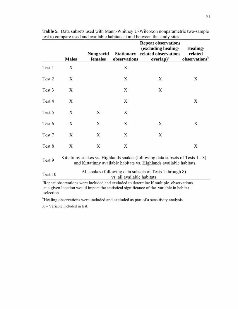
91
Table 5. Data subsets used with Mann-Whitney U-Wilcoxon nonparametric two-sample test to compare used and available habitats at and between the study sites.
Males Nongravid
females Stationary
observations
Repeat observations (excluding healing-
related observations overlap)a
Healing-related
observationsb
Test 1 X X
Test 2 X X X X
Test 3 X X X
Test 4 X X X
Test 5 X X X
Test 6 X X X X X
Test 7 X X X X
Test 8 X X X X
Test 9 Kittatinny snakes vs. Highlands snakes (following data subsets of Tests 1 - 8) and Kittatinny available habitats vs. Highlands available habitats.
Test 10 All snakes (following data subsets of Tests 1 through 8) vs. all available habitats
aRepeat observations were included and excluded to determine if multiple observations at a given location would impact the statistical significance of the variable in habitat selection. bHealing observations were included and excluded as part of a sensitivity analysis. X = Variable included in test.
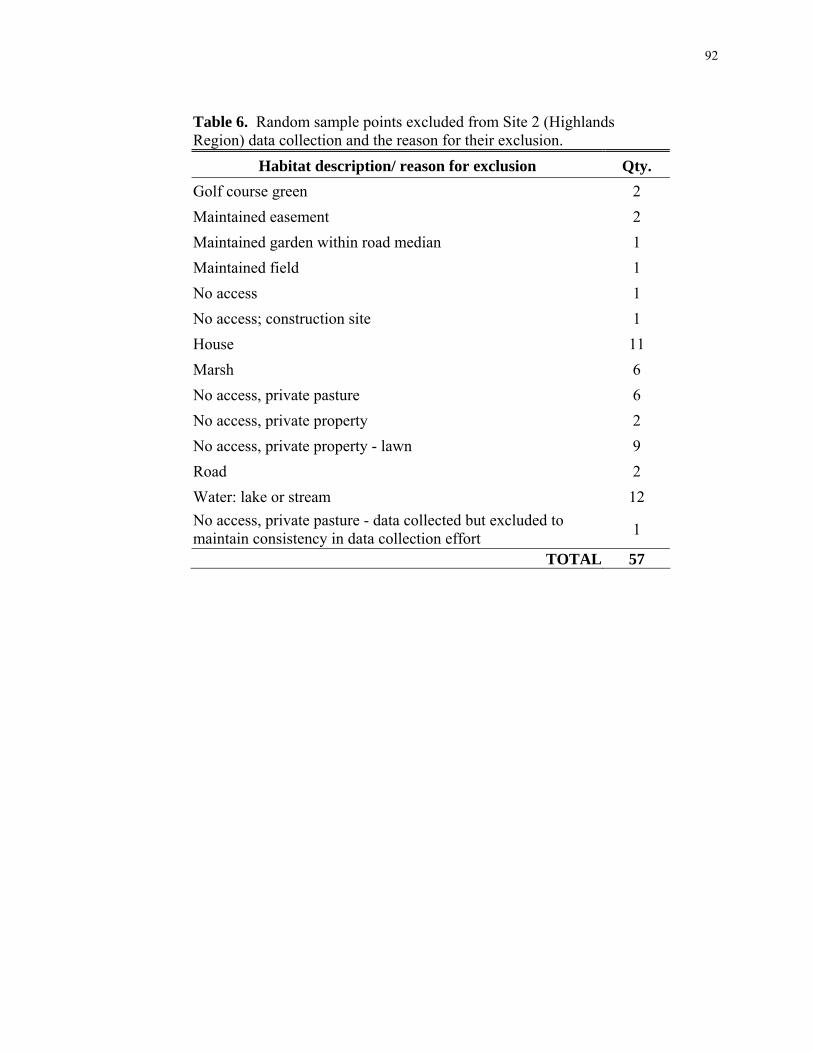
92
Table 6. Random sample points excluded from Site 2 (Highlands Region) data collection and the reason for their exclusion.
Habitat description/ reason for exclusion Qty. Golf course green 2 Maintained easement 2 Maintained garden within road median 1 Maintained field 1 No access 1 No access; construction site 1 House 11 Marsh 6 No access, private pasture 6 No access, private property 2 No access, private property - lawn 9 Road 2 Water: lake or stream 12 No access, private pasture - data collected but excluded to maintain consistency in data collection effort 1
TOTAL 57

93
Table 7a. Results of Mann-Whitney U-Wilcoxon nonparametric two-sample test on used versus available habitats within the Kittatinny Ridge study site (α = 0.05).
Observations included in analysis Sex Distance to
rock Distance to
log
Distance to overstory
tree
DBH of (same)
overstory tree
Distance to understory
tree Slope
Test 1. All stationary observations including repetitive & healing-related locations.
♂
z = 3.0412; p = 0.0024 (Sn = 352; Rn = 83)
z = 2.8508; p = 0.0044 (Sn = 414; Rn = 89)
z = -3.2271; p = 0.0013 (Sn = 421; Rn = 93)
- - -
Test 2. Stationary observations excluding both repetitive & healing-related locations.
♂
z = 2.1456; p = 0.0160 (Sn = 233; Rn = 83)
z = 3.3761; p = 0.0004 (Sn = 270; Rn = 89)
z = -2.1245; p = 0.0168 (Sn = 273; Rn = 93)
- - -
Test 3. Stationary observations including repetitive observations, but excluding healing-related locations.
♂
z = 2.2742; p = 0.0230 (Sn = 302; Rn = 83)
z = 3.6352; p = 0.0003 (Sn = 345; Rn = 89)
z = -2.3197; p = 0.0204 (Sn = 348; Rn = 93)
- - -
Test 4. Stationary observations including healing-related observations, but excluding repetitive locations.
♂
z = 2.5259; p = 0.0115 (Sn = 252; Rn = 83)
z = 2.9545; p = 0.0031 (Sn = 296; Rn = 89)
z = -2.4671; p = 0.0136 (Sn = 302; Rn = 93)
- - -
Test 5. All stationary observations including repetitive & healing-related locations.
♂, ♀
z = 3.2964; p = 0.0010 (Sn = 537; Rn = 83)
z = 3.0753; p = 0.0021 (Sn = 593; Rn = 89)
z = -3.0650; p = 0.0022 (Sn = 596; Rn = 93)
- - -
Test 6. Stationary observations excluding both repetitive & healing-related locations.
♂, ♀
z = 1.9930; p = 0.0463 (Sn = 344; Rn = 83)
z = 3.5360; p = 0.0004 (Sn = 381; Rn = 89)
- - - -
Test 7. Stationary observations including repetitive observations, but excluding healing-related locations.
♂, ♀
z = 2.2476; p = 0.0246 (Sn = 462; Rn = 83)
z = 3.7990; p = 0.0001 (Sn = 506; Rn = 89)
z = -2.3977; p = 0.0165 (Sn = 505; Rn = 93)
- - -
Test 8. Stationary observations including healing-related observations, but excluding repetitive locations.
♂, ♀
z = 2.5271; p = 0.0115 (Sn = 372; Rn = 83)
z = 3.2037; p = 0.0014 (Sn = 414; Rn = 89)
z = -2.1060; p = 0.0352 (Sn = 419; Rn = 93)
- - -
Sn = Snake observations’ sample size Rn = Random locations’ sample size - = Not statistically different

94
Table 7b. Results of Mann-Whitney U-Wilcoxon nonparametric two-sample test on used versus available habitats within the Highlands Region study site (α = 0.05).
Observations included in analysis Sex Distance to
rock Distance to
log
Distance to overstory
tree
DBH of (same)
overstory tree
Distance to understory
tree Slope
Test 1. All stationary observations including repetitive & healing-related locations.
♂
z = 5.4148; p < .0001 (Sn = 481; Rn = 237)
z = 5.0480; p < .0001 (Sn = 483; Rn = 246)
-
z = 4.4553; p < .0001 (Sn = 479; Rn = 251)
-
z = -3.7452; p < .0001 (Sn = 429; Rn = 249)
Test 2. Stationary observations excluding both repetitive & healing-related locations.
♂ -
z = -5.4237; p < .0001 (Sn = 235; Rn = 246)
-
z = -3.8332; p < .0001 (Sn = 234; Rn = 251)
z = -2.7311; p = 0.0063 (Sn = 235; Rn = 251)
-
Test 3. Stationary observations including repetitive observations, but excluding healing-related locations.
♂
z = 3.7372; p = 0.0002 (Sn = 299; Rn = 231)
z = 4.5645; p < .0001 (Sn = 300; Rn = 246)
-
z = 4.0516; p < .0001 (Sn = 299; Rn = 251)
-
z = -3.1145; p = 0.0009 (Sn = 286; Rn = 249)
Test 4. Stationary observations including healing-related observations, but excluding repetitive locations.
♂
z = 2.0692; p = 0.0193 (Sn = 332; Rn = 237)
z = 5.7961; p < .0001 (Sn = 334; Rn = 246)
-
z = 3.6761; p = 0.0002 (Sn = 330; Rn = 251)
z = 2.3261; p = 0.0200 (Sn = 334; Rn = 251)
z = -2.4679; p = 0.0136 (Sn = 291; Rn = 249)
Test 5. All stationary observations including repetitive & healing-related locations.
♂, ♀
z = 5.6386; p < .0001 (Sn = 512; Rn = 237)
z = 5.1704; p < .0001 (Sn = 513; Rn = 246)
-
z = 4.8337; p < .0001 (Sn = 510; Rn = 251)
-
z = -4.2188; p < .0001 (Sn = 460; Rn = 249)
Test 6. Stationary observations excluding both repetitive & healing-related locations.
♂, ♀
z = 2.0722; p = 0.0191 (Sn = 254; Rn = 237)
z = 5.6435; p < .0001 (Sn = 254; Rn = 246)
-
z = 4.2361; p < .0001 (Sn = 254; Rn = 251)
z = 2.6204; p = 0.0088 (Sn = 255; Rn = 251)
z = 2.4852; p = 0.0129 (Sn = 243; Rn = 249)
Test 7. Stationary observations including repetitive observations, but excluding healing-related locations.
♂, ♀
z = 4.1895; p < .0001 (Sn = 329; Rn = 237)
z = 4.7360; p < .0001 (Sn = 329; Rn = 246)
-
z = 4.5648; p < .0001 (Sn = 329; Rn = 251)
-
z = -3.7589; p = 0.0002 (Sn = 316; Rn = 249)
Test 8. Stationary observations including healing-related observations, but excluding repetitive locations.
♂, ♀
z = 2.4882; p = 0.0128 (Sn = 352; Rn = 237)
z = 5.9561; p < .0001 (Sn = 353; Rn = 246)
-
z = 4.0020; p < .0001 (Sn = 350; Rn = 251)
z = 2.2613; p = 0.0237 (Sn = 354; Rn = 251)
z = -2.9731; p = 0.0029 (Sn = 311; Rn = 249)
Sn = Snake observations’ sample size Rn = Random locations’ sample size - = Not statistically different

95
Table 7c. Results of Mann-Whitney U-Wilcoxon nonparametric two-sample test comparing used habitats of the Kitattinny Ridge versus Highlands Region study sites (α = 0.05).
Observations included in analysis Sex Distance to
rock Distance to
log
Distance to overstory
tree
DBH of (same)
overstory tree
Distance to understory
tree Slope
Test 1. All stationary observations including repetitive & healing-related locations.
♂
z = 5.4779; p < .0001
(Sn @ Kittatinny = 352; Sn @
Highlands = 481)
-
z = 4.4959; p < .0001
(Sn @ Kittatinny = 421; Sn @
Highlands = 485)
z = 4.8209; p < .0001
(Sn @ Kittatinny = 420; Sn @
Highlands = 479)
z = 10.5716; p < .0001
(Sn @ Kittatinny = 422; Sn @
Highlands = 481)
z = -12.1546; p < .0001
(Sn @ Kittatinny = 243; Sn @
Highlands = 429)
Test 2. Stationary observations excluding both repetitive & healing-related locations.
♂
z = 2.8151; p = 0.0049
(Sn @ Kittatinny = 233; Sn @
Highlands = 234)
-
z = -2.3920; p = 0.0168
(Sn @ Kittatinny = 273; Sn @
Highlands = 236)
z = -4.6035; p < .0001
(Sn @ Kittatinny = 272; Sn @
Highlands = 234)
z = -10.1364; p < .0001
(Sn @ Kittatinny = 274; Sn @
Highlands = 235)
z = -8.2144; p < .0001
(Sn @ Kittatinny = 133; Sn @
Highlands = 223)
Test 3. Stationary observations including repetitive observations, but excluding healing-related locations.
♂
z = -4.7753; p < .0001
(Sn @ Kittatinny = 302; Sn @
Highlands = 299)
z = 1.9956; p = 0.0460
(Sn @ Kittatinny = 345; Sn @
Highlands = 300)
z = -2.0479; p = 0.0406
(Sn @ Kittatinny = 348; Sn @
Highlands = 301)
z = -4.4569; p < .0001
(Sn @ Kittatinny = 347; Sn @
Highlands = 399)
z = -9.7149; p < .0001
(Sn @ Kittatinny = 349; Sn @
Highlands = 298)
z = -10.5160; p < .0001
(Sn @ Kittatinny = 188; Sn @
Highlands = 286)
Test 4. Stationary observations including healing-related observations, but excluding repetitive locations.
♂
z = 2.9855; p = 0.0028
(Sn @ Kittatinny = 252; Sn @
Highlands = 332)
-
z = 2.4077; p = 0.0161
(Sn @ Kittatinny = 302; Sn @
Highlands = 336)
z = 4.3481; p < .0001
(Sn @ Kittatinny = 301; Sn @
Highlands = 330)
z = 10.4420; p < .0001
(Sn @ Kittatinny = 303; Sn @
Highlands = 334)
z = -8.9712; p < .0001
(Sn @ Kittatinny = 156; Sn @
Highlands = 291)
Test 5. All stationary observations including repetitive & healing-related locations.
♂, ♀ -
z = -4.5274; p < .0001
(Sn @ Kittatinny = 596; Sn @
Highlands = 515)
z = -5.0376; p < .0001
(Sn @ Kittatinny = 596; Sn @
Highlands = 510)
z = -12.8988; p < .0001
(Sn @ Kittatinny = 601; Sn @
Highlands = 512)
z = 10.4420; p < .0001
(Sn @ Kittatinny = 303; Sn @
Highlands = 334)
z = -12.9039; p < .0001
(Sn @ Kittatinny = 358; Sn @
Highlands = 460)
Test 6. Stationary observations excluding both repetitive & healing-related locations.
♂, ♀
z = -4.1257; p < .0001
(Sn @ Kittatinny = 344; Sn @
Highlands = 254)
-
z = -2.2283; p = 0.0259
(Sn @ Kittatinny = 383; Sn @
Highlands = 256)
z = -4.4800; p < .0001
(Sn @ Kittatinny = 383; Sn @
Highlands = 254)
z = -11.4027; p < .0001
(Sn @ Kittatinny = 385; Sn @
Highlands = 255)
z = -8.8639; p < .0001
(Sn @ Kittatinny = 197; Sn @
Highlands = 243)
Sn = Snake observations’ sample size - = Not statistically different
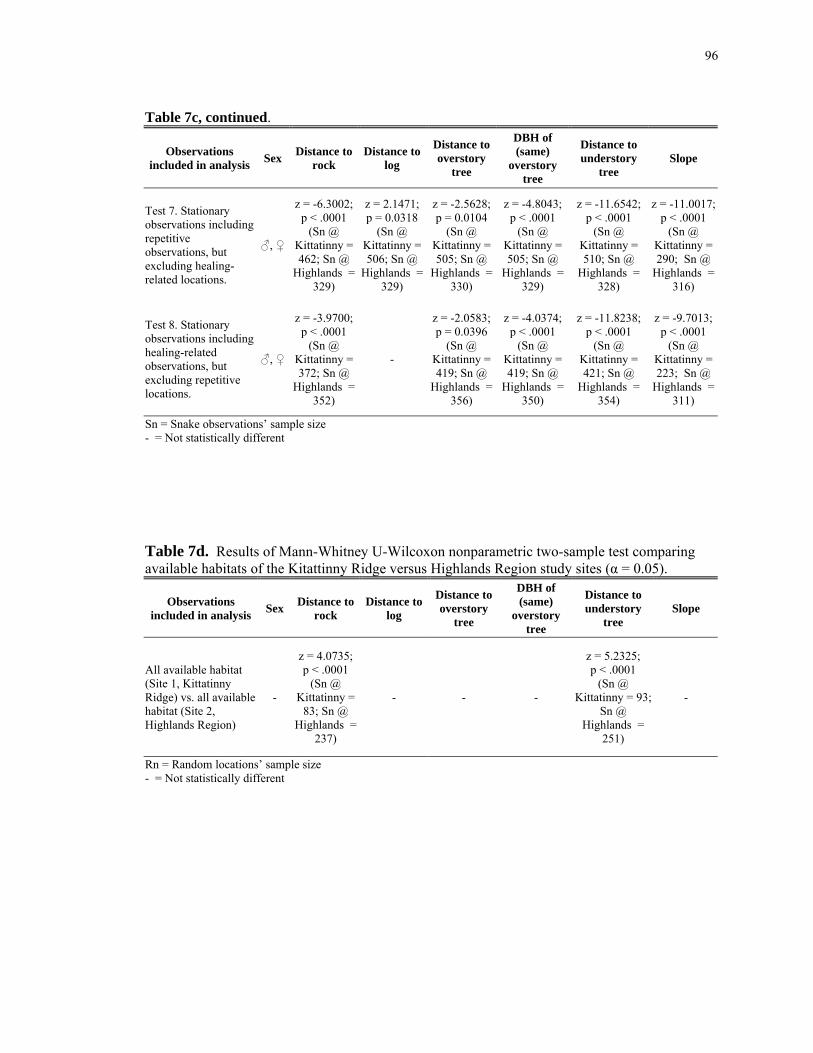
96
Table 7c, continued.
Observations included in analysis Sex Distance to
rock Distance to
log
Distance to overstory
tree
DBH of (same)
overstory tree
Distance to understory
tree Slope
Test 7. Stationary observations including repetitive observations, but excluding healing-related locations.
♂, ♀
z = -6.3002; p < .0001
(Sn @ Kittatinny = 462; Sn @
Highlands = 329)
z = 2.1471; p = 0.0318
(Sn @ Kittatinny = 506; Sn @
Highlands = 329)
z = -2.5628; p = 0.0104
(Sn @ Kittatinny = 505; Sn @
Highlands = 330)
z = -4.8043; p < .0001
(Sn @ Kittatinny = 505; Sn @
Highlands = 329)
z = -11.6542; p < .0001
(Sn @ Kittatinny = 510; Sn @
Highlands = 328)
z = -11.0017; p < .0001
(Sn @ Kittatinny = 290; Sn @
Highlands = 316)
Test 8. Stationary observations including healing-related observations, but excluding repetitive locations.
♂, ♀
z = -3.9700; p < .0001
(Sn @ Kittatinny = 372; Sn @
Highlands = 352)
-
z = -2.0583; p = 0.0396
(Sn @ Kittatinny = 419; Sn @
Highlands = 356)
z = -4.0374; p < .0001
(Sn @ Kittatinny = 419; Sn @
Highlands = 350)
z = -11.8238; p < .0001
(Sn @ Kittatinny = 421; Sn @
Highlands = 354)
z = -9.7013; p < .0001
(Sn @ Kittatinny = 223; Sn @
Highlands = 311)
Sn = Snake observations’ sample size - = Not statistically different
Table 7d. Results of Mann-Whitney U-Wilcoxon nonparametric two-sample test comparing available habitats of the Kitattinny Ridge versus Highlands Region study sites (α = 0.05).
Observations included in analysis Sex Distance to
rock Distance to
log
Distance to overstory
tree
DBH of (same)
overstory tree
Distance to understory
tree Slope
All available habitat (Site 1, Kittatinny Ridge) vs. all available habitat (Site 2, Highlands Region)
-
z = 4.0735; p < .0001
(Sn @ Kittatinny =
83; Sn @ Highlands =
237)
- - -
z = 5.2325; p < .0001
(Sn @ Kittatinny = 93;
Sn @ Highlands =
251)
-
Rn = Random locations’ sample size - = Not statistically different
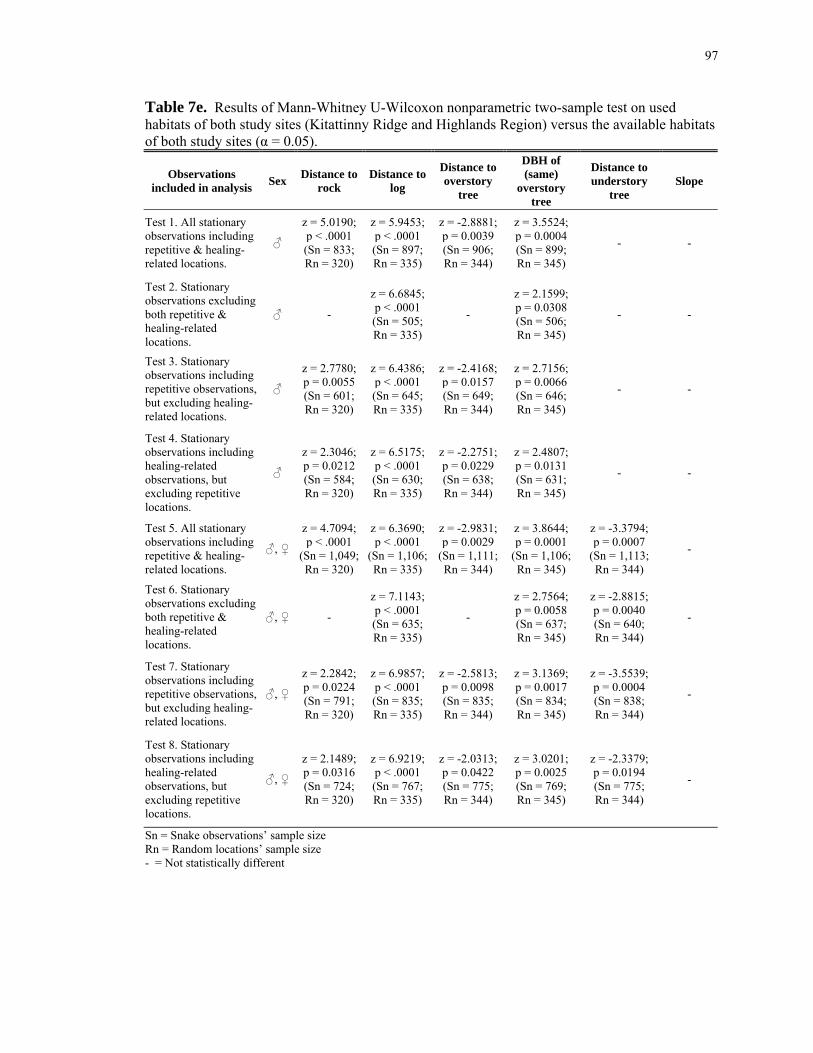
97
Table 7e. Results of Mann-Whitney U-Wilcoxon nonparametric two-sample test on used habitats of both study sites (Kitattinny Ridge and Highlands Region) versus the available habitats of both study sites (α = 0.05).
Observations included in analysis Sex Distance to
rock Distance to
log
Distance to overstory
tree
DBH of (same)
overstory tree
Distance to understory
tree Slope
Test 1. All stationary observations including repetitive & healing-related locations.
♂
z = 5.0190; p < .0001 (Sn = 833; Rn = 320)
z = 5.9453; p < .0001 (Sn = 897; Rn = 335)
z = -2.8881; p = 0.0039 (Sn = 906; Rn = 344)
z = 3.5524; p = 0.0004 (Sn = 899; Rn = 345)
- -
Test 2. Stationary observations excluding both repetitive & healing-related locations.
♂ -
z = 6.6845; p < .0001 (Sn = 505; Rn = 335)
-
z = 2.1599; p = 0.0308 (Sn = 506; Rn = 345)
- -
Test 3. Stationary observations including repetitive observations, but excluding healing-related locations.
♂
z = 2.7780; p = 0.0055 (Sn = 601; Rn = 320)
z = 6.4386; p < .0001 (Sn = 645; Rn = 335)
z = -2.4168; p = 0.0157 (Sn = 649; Rn = 344)
z = 2.7156; p = 0.0066 (Sn = 646; Rn = 345)
- -
Test 4. Stationary observations including healing-related observations, but excluding repetitive locations.
♂
z = 2.3046; p = 0.0212 (Sn = 584; Rn = 320)
z = 6.5175; p < .0001 (Sn = 630; Rn = 335)
z = -2.2751; p = 0.0229 (Sn = 638; Rn = 344)
z = 2.4807; p = 0.0131 (Sn = 631; Rn = 345)
- -
Test 5. All stationary observations including repetitive & healing-related locations.
♂, ♀
z = 4.7094; p < .0001
(Sn = 1,049; Rn = 320)
z = 6.3690; p < .0001
(Sn = 1,106; Rn = 335)
z = -2.9831; p = 0.0029
(Sn = 1,111; Rn = 344)
z = 3.8644; p = 0.0001
(Sn = 1,106; Rn = 345)
z = -3.3794; p = 0.0007
(Sn = 1,113; Rn = 344)
-
Test 6. Stationary observations excluding both repetitive & healing-related locations.
♂, ♀ -
z = 7.1143; p < .0001 (Sn = 635; Rn = 335)
-
z = 2.7564; p = 0.0058 (Sn = 637; Rn = 345)
z = -2.8815; p = 0.0040 (Sn = 640; Rn = 344)
-
Test 7. Stationary observations including repetitive observations, but excluding healing-related locations.
♂, ♀
z = 2.2842; p = 0.0224 (Sn = 791; Rn = 320)
z = 6.9857; p < .0001 (Sn = 835; Rn = 335)
z = -2.5813; p = 0.0098 (Sn = 835; Rn = 344)
z = 3.1369; p = 0.0017 (Sn = 834; Rn = 345)
z = -3.5539; p = 0.0004 (Sn = 838; Rn = 344)
-
Test 8. Stationary observations including healing-related observations, but excluding repetitive locations.
♂, ♀
z = 2.1489; p = 0.0316 (Sn = 724; Rn = 320)
z = 6.9219; p < .0001 (Sn = 767; Rn = 335)
z = -2.0313; p = 0.0422 (Sn = 775; Rn = 344)
z = 3.0201; p = 0.0025 (Sn = 769; Rn = 345)
z = -2.3379; p = 0.0194 (Sn = 775; Rn = 344)
-
Sn = Snake observations’ sample size Rn = Random locations’ sample size - = Not statistically different

98
Table 8a. Results of Mann-Whitney U-Wilcoxon nonparametric two-sample test on used versus available habitats within study site 1 (Kittatinny Ridge) for proximities to water, human activity, forest edge and roads (α = 0.05). Random habitats at Site 1, n = 1,793.
Observations included in analysis Sex Proximity to water
Proximity to human activity
Proximity to forest edge
Proximity to roads
Test 1. All stationary observations including repetitive & healing-related locations. (Snakes, n = 198)
♂ - z = 2.5667; p = 0.0103
z = -2.4860; p = 0.0129
z = 11.3159; p < .0001
Test 2. Stationary observations excluding both repetitive & healing-related locations. (Snakes, n = 142)
♂ - z = 2.5656; p = 0.0103 - z = 8.4491;
p < .0001
Test 3. Stationary observations including repetitive observations, but excluding healing-related locations. (Snakes, n = 185)
♂ - z = 3.1132; p = 0.0019 - z = 10.4942;
p < .0001
Test 4. Stationary observations including healing-related observations, but excluding repetitive locations. (Snakes, n = 147)
♂ - z = 2.4345; p < 0.0149 - z = 8.1019;
p < .0001
Test 5. All stationary observations including repetitive & healing-related locations. (Snakes, n = 283)
♂, ♀ - z = 6.0866; p < .0001 - z = 14.8608;
p < .0001
Test 6. Stationary observations excluding both repetitive & healing-related locations. (Snakes, n = 184)
♂, ♀ - z = 4.8693; p < .0001 - z = 11.2424;
p < .0001
Test 7. Stationary observations including repetitive observations, but excluding healing-related locations. (Snakes, n = 249)
♂, ♀ - z = 6.1782; p < .0001 - z = 13.8461;
p < .0001
Test 8. Stationary observations including healing-related observations, but excluding repetitive locations. (Snakes, n = 195)
♂, ♀ - z = 4.9173; p < .0001 - z = 11.1061;
p < .0001
n = sample size - = Not statistically different

99
Table 8b. Results of Mann-Whitney U-Wilcoxon nonparametric two-sample test on used versus available habitats within study site 2 (Highlands Region) for proximities to water, human activity, forest edge and roads (α = 0.05). Random habitats at Site 2, n = 10,799.
Observations included in analysis Sex Proximity to water
Proximity to human activity
Proximity to forest edge
Proximity to roads
Test 1. All stationary observations including repetitive & healing-related locations. (Snakes, n = 525)
♂ z = 4.1215; p < .0001
z = 8.9261; p < .0001
z = 2.5124; p = 0.0120
z = 14.5786; p < .0001
Test 2. Stationary observations excluding both repetitive & healing-related locations. (Snakes, n = 232)
♂ z = 4.0502; p < .0001
z = 2.3680; p = 0.0179 - z = 4.8912;
p < .0001
Test 3. Stationary observations including repetitive observations, but excluding healing-related locations. (Snakes, n = 330)
♂ z = 4.8399; p < .0001
z = 3.6221; p = 0.0003 - z = 6.4120;
p < .0001
Test 4. Stationary observations including healing-related observations, but excluding repetitive locations. (Snakes, n = 339)
♂ z = 2.8089; p = 0.0050
z = 5.3747; p < .0001
z = 2.4952; p < 0.0126
z = 8.8392; p < .0001
Test 5. All stationary observations including repetitive & healing-related locations. (Snakes, n = 557)
♂, ♀ z = 4.9142; p < .0001
z = 9.5212; p < .0001 - z = 13.8362;
p < .0001
Test 6. Stationary observations excluding both repetitive & healing-related locations. (Snakes, n = 251)
♂, ♀ z = 4.6120; p < .0001
z = 3.0055; p = 0.0027 - z = 4.2952;
p < .0001
Test 7. Stationary observations including repetitive observations, but excluding healing-related locations. (Snakes, n = 361)
♂, ♀ z = 5.7094; p < .0001
z = 4.5499; p < .0001 - z = 5.6643;
p < .0001
Test 8. Stationary observations including healing-related observations, but excluding repetitive locations. (Snakes, n = 358)
♂, ♀ z = 3.3321; p = 0.0009
z = 5.8347; p < .0001 - z = 8.2581;
p < .0001
n = sample size - = Not statistically different

100
Table 8c. Results of Mann-Whitney U-Wilcoxon nonparametric two-sample test comparing used habitats within the Kitattinny Ridge and Highlands Region study sites for proximities to water, human activity, forest edge and roads (α = 0.05).
Observations included in analysis Sex Proximity to water
Proximity to human activity
Proximity to forest edge
Proximity to roads
Test 1. All stationary observations including repetitive & healing-related locations. (Snakes @ Kittatinny, n = 283; Snakes @ Highlands, n = 557)
♂ - z = -6.2231; p < .0001
z = -5.5549; p < .0001 -
Test 2. Stationary observations excluding both repetitive & healing-related locations. (Snakes @ Kittatinny, n = 142; Snakes @ Highlands, n = 232)
♂ - - z = -3.5077; p = 0.0005
z = 2.7694; p = 0.0056
Test 3. Stationary observations including repetitive observations, but excluding healing-related locations. (Snakes @ Kittatinny, n = 185; Snakes @ Highlands, n = 330)
♂ - z = -1.9849; p = 0.0472
z = 4.3498; p < .0001
z = 3.8014; p = 0.0001
Test 4. Stationary observations including healing-related observations, but excluding repetitive locations. (Snakes @ Kittatinny, n = 147; Snakes @ Highlands, n = 339)
♂ - z = -3.7304; p = 0.0002
z = -4.3678; p < .0001 -
Test 5. All stationary observations including repetitive & healing-related locations. (Snakes @ Kittatinny, n = 283; Snakes @ Highlands, n = 557)
♂, ♀ - z = -4.4813; p < .0001
z = -3.0286; p = 0.0025 -
Test 6. Stationary observations excluding both repetitive & healing-related locations. (Snakes @ Kittatinny, n = 184; Snakes @ Highlands, n = 251)
♂, ♀ - - z = -2.1550; p = 0.0312
z = 4.8731; p < .0001
Test 7. Stationary observations including repetitive observations, but excluding healing-related locations. (Snakes @ Kittatinny, n = 249; Snakes @ Highlands, n = 361)
♂, ♀ - - z = -2.3694; p = 0.0178
z = 6.3894; p < .0001
Test 8. Stationary observations including healing-related observations, but excluding repetitive locations. (Snakes @ Kittatinny, n = 195; Snakes @ Highlands, n = 358)
♂, ♀ - z = -2.3019; p = 0.0213
z = -3.0305; p = 0.0024
z = 2.1994; p = 0.0278
n = sample size - = Not statistically different

101
Table 8d. Results of Mann-Whitney U-Wilcoxon nonparametric two-sample test comparing available habitats within the Kitattinny Ridge and Highlands Region study sites for proximities to water, human activity, forest edge and roads (α = 0.05). Random habitats at Site 1, Kittatinny Ridge, n = 1,793; random habitats at Site 2, Highlands Region, n = 10,799.
Observations included in analysis Sex Proximity to water
Proximity to human activity
Proximity to forest edge
Proximity to roads
All available habitat (Site 1) vs. all available habitat (Site 2) - z = 9.9599;
p < .0001 z = -3.5277; p = 0.0004
z = -10.6953; p < .0001 -
n = sample size - = Not statistically different

102
Table 8e. Results of Mann-Whitney U-Wilcoxon nonparametric two-sample test on used habitats of both study sites (Kitattinny Ridge and Highlands Region) versus the available habitats of both study sites for proximities to water, human activity, forest edge and roads (α = 0.05).
Observations included in analysis Sex Proximity to water
Proximity to human activity
Proximity to forest edge
Proximity to roads
Test 1. All stationary observations including repetitive & healing-related locations. (Snakes, n = 722; Random, n = 12,592)
♂ z = 3.6248; p = 0.0003
z = 8.6805; p < .0001 - z = 17.4994;
p < .0001
Test 2. Stationary observations excluding both repetitive & healing-related locations. (Snakes, n = 355; Random, n = 12,592)
♂ z = 3.9956; p < .0001
z = 3.3334; p = 0.0009 - z = 9.4688;
p < .0001
Test 3. Stationary observations including repetitive observations, but excluding healing-related locations. (Snakes, n = 488; Random, n = 12,592)
♂ z = 4.5218; p < .0001
z = 4.4715; p < .0001 - z = 11.4956;
p < .0001
Test 4. Stationary observations including healing-related observations, but excluding repetitive locations. (Snakes, n = 486; Random, n = 12,592)
♂ z = 2.5191; p = 0.0118
z = 5.5017; p < .0001 - z = 11.1779;
p < .0001
Test 5. All stationary observations including repetitive & healing-related locations. (Snakes, n = 839; Random, n = 12,592)
♂, ♀ z = 5.7346; p < .0001
z = 10.6535; p < .0001 - z = 18.7284;
p < .0001
Test 6. Stationary observations excluding both repetitive & healing-related locations. (Snakes, n = 416; Random, n = 12,592)
♂, ♀ z = 5.8072; p < .0001
z = 5.1150; p < .0001 - z = 10.6101;
p < .0001
Test 7. Stationary observations including repetitive observations, but excluding healing-related locations. (Snakes, n = 582; Random, n = 12,592)
♂, ♀ z = 7.0987; p < .0001
z = 6.8494; p < .0001 - z = 12.8566;
p < .0001
Test 8. Stationary observations including healing-related observations, but excluding repetitive locations. (Snakes, n = 553; Random, n = 12,592)
♂, ♀ z = 4.2088; p < .0001
z = 7.0355; p < .0001 - z = 12.2773;
p < .0001
n = sample size

103
Table 8f. Results of Mann-Whitney U-Wilcoxon nonparametric two-sample test on used versus available habitats within Site 1 (Kittatinny Ridge) for canopy closure (α = 0.05).
Observations included in analysis Sex Canopy closure
Test 1. All stationary observations including repetitive & healing-related locations. (Snakes, n = 417; Random, n = 93) ♂ z = 4.3154;
p < .0001
Test 2. Stationary observations excluding both repetitive & healing-related locations. (Snakes, n = 273; Random, n = 93) ♂ z = 2.5172;
p = 0.0118
Test 3. Stationary observations including repetitive observations, but excluding healing-related locations. (Snakes, n = 344; Random, n = 93)
♂ z = 3.0927; p = 0.0020
Test 4. Stationary observations including healing-related observations, but excluding repetitive locations. (Snakes, n = 302; Random, n = 93)
♂ z = 3.1636; p = 0.0016
Test 5. All stationary observations including repetitive & healing-related locations. (Snakes, n = 594; Random, n = 93) ♂, ♀ z = 4.2612;
p < .0001
Test 6. Stationary observations excluding both repetitive & healing-related locations. (Snakes, n = 385; Random, n = 93)
♂, ♀ z = 2.4008; p = 0.0164
Test 7. Stationary observations including repetitive observations, but excluding healing-related locations. (Snakes, n = 506; Random, n = 93)
♂, ♀ z = 3.1712; p = 0.0015
Test 8. Stationary observations including healing-related observations, but excluding repetitive locations. (Snakes, n = 421; Random, n = 93)
♂, ♀ z = 3.0360; p = 0.0024
n = sample size

104
Table 8g. Results of Mann-Whitney U-Wilcoxon nonparametric two-sample test on used versus available habitats within Site 2 (Highlands Region) for canopy closure (α = 0.05).
Observations included in analysis Sex Canopy closure
Test 1. All stationary observations including repetitive & healing-related locations. (Snakes, n = 484; Random, n = 246) ♂ z = 7.6390;
p < .0001
Test 2. Stationary observations excluding both repetitive & healing-related locations. (Snakes, n = 235; Random, n = 246) ♂ z = -4.5717;
p < .0001
Test 3. Stationary observations including repetitive observations, but excluding healing-related locations. (Snakes, n = 300; Random, n = 246)
♂ z = 6.2739; p < .0001
Test 4. Stationary observations including healing-related observations, but excluding repetitive locations. (Snakes, n = 335; Random, n = 246)
♂ z = 4.8541; p < .0001
Test 5. All stationary observations including repetitive & healing-related locations. (Snakes, n = 515; Random, n = 246) ♂, ♀ z = 7.7801;
p < .0001
Test 6. Stationary observations excluding both repetitive & healing-related locations. (Snakes, n = 255; Random, n = 246) ♂, ♀ z = 4.8506;
p < .0001
Test 7. Stationary observations including repetitive observations, but excluding healing-related locations. (Snakes, n = 330; Random, n = 246)
♂, ♀ z = 6.5381; p < .0001
Test 8. Stationary observations including healing-related observations, but excluding repetitive locations. (Snakes, n = 355; Random, n = 246)
♂, ♀ z = 5.0621; p < .0001
n = sample size
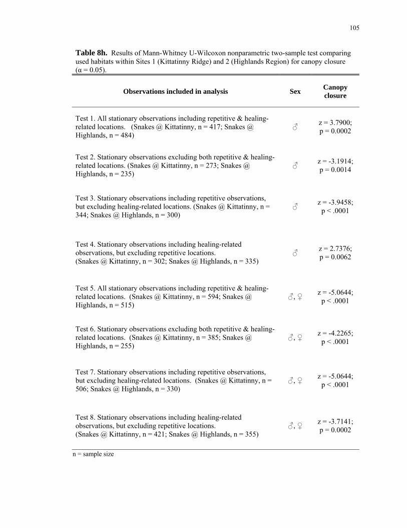
105
Table 8h. Results of Mann-Whitney U-Wilcoxon nonparametric two-sample test comparing used habitats within Sites 1 (Kittatinny Ridge) and 2 (Highlands Region) for canopy closure (α = 0.05).
Observations included in analysis Sex Canopy closure
Test 1. All stationary observations including repetitive & healing-related locations. (Snakes @ Kittatinny, n = 417; Snakes @ Highlands, n = 484)
♂ z = 3.7900; p = 0.0002
Test 2. Stationary observations excluding both repetitive & healing-related locations. (Snakes @ Kittatinny, n = 273; Snakes @ Highlands, n = 235)
♂ z = -3.1914; p = 0.0014
Test 3. Stationary observations including repetitive observations, but excluding healing-related locations. (Snakes @ Kittatinny, n = 344; Snakes @ Highlands, n = 300)
♂ z = -3.9458; p < .0001
Test 4. Stationary observations including healing-related observations, but excluding repetitive locations. (Snakes @ Kittatinny, n = 302; Snakes @ Highlands, n = 335)
♂ z = 2.7376; p = 0.0062
Test 5. All stationary observations including repetitive & healing-related locations. (Snakes @ Kittatinny, n = 594; Snakes @ Highlands, n = 515)
♂, ♀ z = -5.0644; p < .0001
Test 6. Stationary observations excluding both repetitive & healing-related locations. (Snakes @ Kittatinny, n = 385; Snakes @ Highlands, n = 255)
♂, ♀ z = -4.2265; p < .0001
Test 7. Stationary observations including repetitive observations, but excluding healing-related locations. (Snakes @ Kittatinny, n = 506; Snakes @ Highlands, n = 330)
♂, ♀ z = -5.0644; p < .0001
Test 8. Stationary observations including healing-related observations, but excluding repetitive locations. (Snakes @ Kittatinny, n = 421; Snakes @ Highlands, n = 355)
♂, ♀ z = -3.7141; p = 0.0002
n = sample size

106
Table 8i. Results of Mann-Whitney U-Wilcoxon nonparametric two-sample test comparing available habitats within Sites 1 (Kittatinny Ridge) and 2 (Highlands Region) for canopy closure (α = 0.05).
Observations included in analysis Sex Canopy closure
All available habitat (Site 1) vs. all available habitat (Site 2). (Snakes @ Kittatinny, n = 93; Snakes @ Highlands, n = 246) - z = 2.7835;
p = 0.0054
n = sample size - = Not applicable
Table 8j. Results of Mann-Whitney U-Wilcoxon nonparametric two-sample test on used habitats of both study sites (Kitattinny Ridge and Highlands Region) versus the available habitats of both study sites for canopy closure (α = 0.05).
Observations included in analysis Sex Canopy closure
Test 1. All stationary observations including repetitive & healing-related locations. (Snakes, n = 901; Random, n = 339) ♂ z = 8.0847;
p < .0001
Test 2. Stationary observations excluding both repetitive & healing-related locations. (Snakes, n = 508; Random, n = 339) ♂ z = 4.1349;
p < .0001
Test 3. Stationary observations including repetitive observations, but excluding healing-related locations. (Snakes, n = 644; Random, n = 339)
♂ z =5.7734; p < .0001
Test 4. Stationary observations including healing-related observations, but excluding repetitive locations. (Snakes, n = 637; Random, n = 339)
♂ z = 5.1612; p < .0001
Test 5. All stationary observations including repetitive & healing-related locations. (Snakes, n = 1,109; Random, n = 339) ♂, ♀ z = 7.8314;
p < .0001
Test 6. Stationary observations excluding both repetitive & healing-related locations. (Snakes, n = 640; Random, n = 339) ♂, ♀ z = 3.8155;
p = 0.0001
Test 7. Stationary observations including repetitive observations, but excluding healing-related locations. (Snakes, n = 836; Random, n = 339)
♂, ♀ z = 5.6198; p < .0001
Test 8. Stationary observations including healing-related observations, but excluding repetitive locations. (Snakes, n = 776; Random, n = 339)
♂, ♀ z = 4.8938; p < .0001
n = sample size

107
Table 8k. Results of Mann-Whitney U-Wilcoxon nonparametric two-sample test on used versus available habitats at Site 2 (Highlands Region) regarding proximity to nearest rock outcrop; random locations (α = 0.05), n = 150.
Observations included in analysis Sex Proximity to nearest rock outcrop, within 50 m (m)
Test 1. All stationary observations including repetitive & healing-related locations. (Snakes, n = 172)
♂ z = 4.3573; p < .0001
Test 2. Stationary observations excluding both repetitive & healing-related locations. (Snakes, n = 353)
♂ z = 7.2827; p < .0001
Test 3. Stationary observations including repetitive observations, but excluding healing-related locations. (Snakes, n = 230)
♂ z = 5.3131; p < .0001
Test 4. Stationary observations including healing-related observations, but excluding repetitive locations. (Snakes, n = 222)
♂ z = 5.1689; p = 0.0050
Test 5. All stationary observations including repetitive & healing-related locations. (Snakes, n = 382)
♂, ♀ z = 7.5420; p < .0001
Test 6. Stationary observations excluding both repetitive & healing-related locations. (Snakes, n = 190)
♂, ♀ z = 4.8599; p < .0001
Test 7. Stationary observations including repetitive observations, but excluding healing-related locations. (Snakes, n = 258)
♂, ♀ z = 5.7504; p < .0001
Test 8. Stationary observations including healing-related observations, but excluding repetitive locations. (Snakes, n = 240)
♂, ♀ z = 5.5605; p = 0.0009
n = sample size

108
Table 9a. Percentage means and 95% CI (2SE) of snake and random locations' canopy closure representing the category containing the largest sample sizes of each group. Used and available canopy closure were statistically different for all subsets of data although the majority of the data collected were captured within Category 5 (81 – 100% canopy closure). Means reveal the snakes selected for slightly more open canopies than what was available to them.
Canopy closure (%) Site 1 Site 2
Category Snake observations
(N = 379)
Random locations (N = 79)
Snake observations
(N = 284)
Random locations (N = 218)
Category 5 93.80 + 0.58 95.37 + 1.16 92.57 + 0.65 93.08 + 0.66
Table 9b. Distance means and 95% CI (2SE) of snake and random locations' proximities to streams and rivers representing the category containing the largest sample sizes of each group. The proximity to streams and rivers showed statistical differences between used and available habitats within the Highlands Region (Site 2) but not along the Kittatinny Ridge (Site 1). The majority of all samples were within 0 – 200m (Category 1) of a stream or river >10m wide. Means reveal the snakes showed a slight aversion to streams and rivers >10m wide.
Proximity to streams and rivers (m) Site 1 Site 2
Category Snake observations
(N = 119)
Random locations (N = 698)
Snake observations
(N = 252)
Random locations
(N = 5338)
Category 1 118.10 + 8.65 99.70 + 4.35 110.07 + 6.54 93.66 + 1.59

109
Table 9c. Distance means and 95% CI (2SE) of snake and random locations' proximities to human-occupied areas representing the categories containing the largest sample sizes of each group. Proximity to human activity/ human-occupied areas was statistically different among all data subsets testing used and available habitat, but varied when comparing snakes between Sites 1 and 2. The majority of the samples collected were captured within Categories 2 (0 – 500m) and 3 (500 – 1000m). Means reveal the snakes showed an aversion to human-occupied areas.
Proximity to human activity/ human-occupied areas (m) Site 1 Site 2
Category Snake observations
(N = 161)
Random locations (N = 970)
Snake observations
(N = 222)
Random locations
(N = 4897)
Category 2 278.54 + 18.37 201.14 + 9.71 - 196.73 + 4.37
Category 3 - - 785.40 + 14.70 -
Table 9d. Distance means and 95% CI (2SE) of snake and random locations' proximities to paved roads representing the categories containing the largest sample sizes of each group. Proximity to roads was statistically different among all data subsets testing used and available habitat, but varied when comparing snakes between Sites 1 and 2. The majority of the samples collected were captured within Categories 1 (0 – 500m) and 3 (1000 – 1500m). Means reveal the snakes showed an aversion to paved roads for stationary behaviors (e.g., foraging, basking, resting).
Proximity to roads (m) Site 1 Site 2
Category Snake observations
(N = 168)
Random locations (N = 928)
Snake observations
(N = 175)
Random locations
(N = 5733)
Category 1 - 222.67 + 9.43 265.87 + 21.13 181.17 + 3.86
Category 3 1165.77 + 14.88 - - -
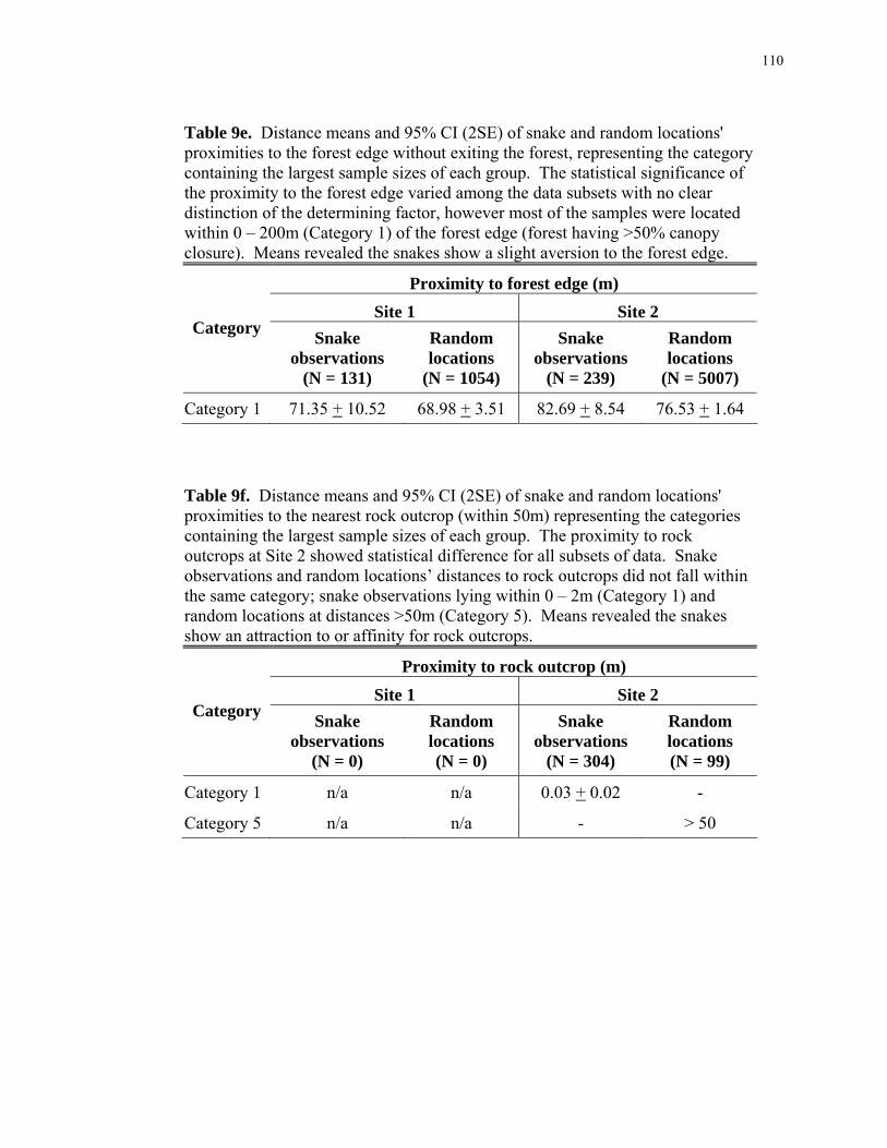
110
Table 9e. Distance means and 95% CI (2SE) of snake and random locations' proximities to the forest edge without exiting the forest, representing the category containing the largest sample sizes of each group. The statistical significance of the proximity to the forest edge varied among the data subsets with no clear distinction of the determining factor, however most of the samples were located within 0 – 200m (Category 1) of the forest edge (forest having >50% canopy closure). Means revealed the snakes show a slight aversion to the forest edge.
Proximity to forest edge (m) Site 1 Site 2
Category Snake observations
(N = 131)
Random locations
(N = 1054)
Snake observations
(N = 239)
Random locations
(N = 5007)
Category 1 71.35 + 10.52 68.98 + 3.51 82.69 + 8.54 76.53 + 1.64
Table 9f. Distance means and 95% CI (2SE) of snake and random locations' proximities to the nearest rock outcrop (within 50m) representing the categories containing the largest sample sizes of each group. The proximity to rock outcrops at Site 2 showed statistical difference for all subsets of data. Snake observations and random locations’ distances to rock outcrops did not fall within the same category; snake observations lying within 0 – 2m (Category 1) and random locations at distances >50m (Category 5). Means revealed the snakes show an attraction to or affinity for rock outcrops.
Proximity to rock outcrop (m) Site 1 Site 2
Category Snake observations
(N = 0)
Random locations (N = 0)
Snake observations
(N = 304)
Random locations (N = 99)
Category 1 n/a n/a 0.03 + 0.02 -
Category 5 n/a n/a - > 50

111
ILLUSTRATIONS
Figure 1. Study area within northern New Jersey.
Highlands Region
Kittatinny Ridge, a portion of the Ridge and Valley Region
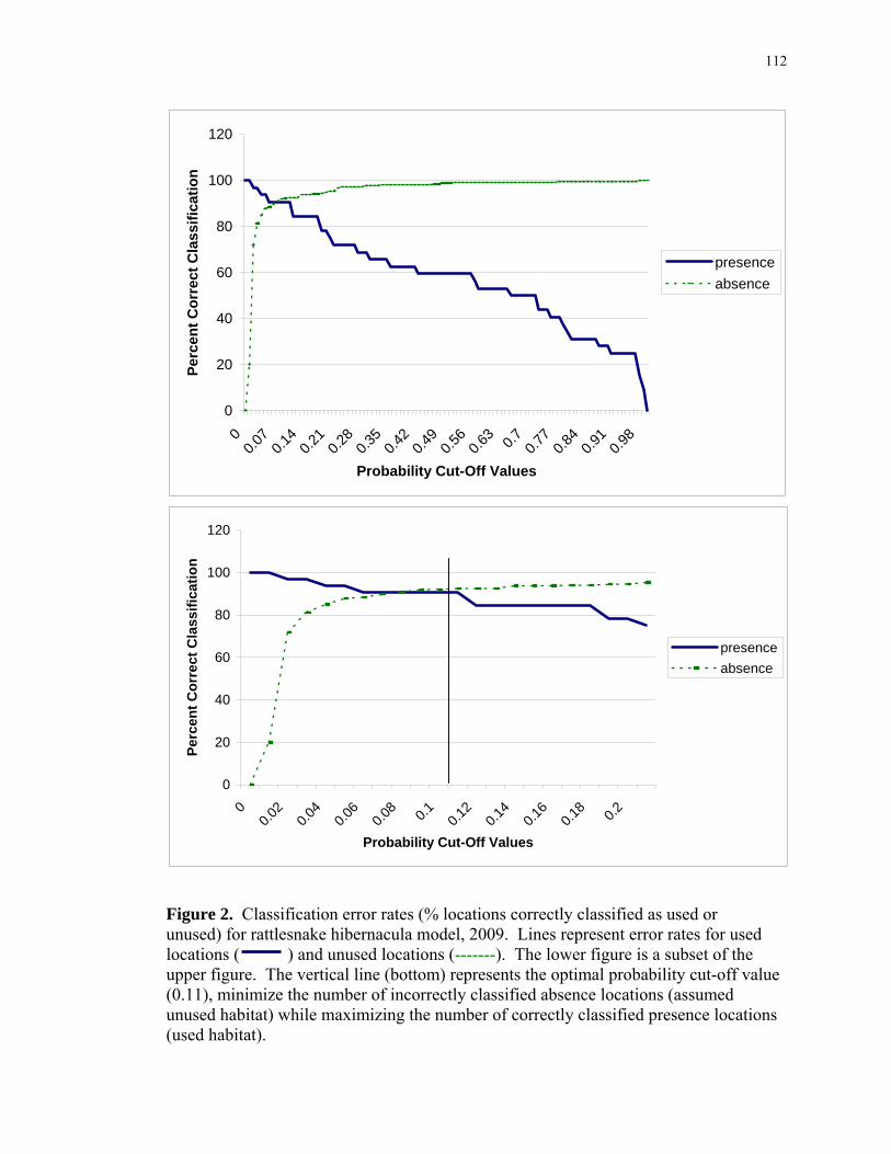
112
0
20
40
60
80
100
120
00.0
20.0
40.0
60.0
8 0.1 0.12
0.14
0.16
0.18 0.2
Probability Cut-Off Values
Perc
ent C
orre
ct C
lass
ifica
tion
presenceabsence
0
20
40
60
80
100
120
00.0
70.1
40.2
10.2
80.3
50.4
20.4
90.5
60.6
3 0.7 0.77
0.84
0.91
0.98
Probability Cut-Off Values
Perc
ent C
orre
ct C
lass
ifica
tion
presenceabsence
Figure 2. Classification error rates (% locations correctly classified as used or unused) for rattlesnake hibernacula model, 2009. Lines represent error rates for used locations ( ) and unused locations (-------). The lower figure is a subset of the upper figure. The vertical line (bottom) represents the optimal probability cut-off value (0.11), minimize the number of incorrectly classified absence locations (assumed unused habitat) while maximizing the number of correctly classified presence locations (used habitat).

113
Figure 3. Map distinguishing suitable versus unsuitable habitat for hibernacula, 2004.

114
Figure 4. Map distinguishing suitable versus unsuitable habitat for hibernacula, 2009.

115
Figure 5. Example of random points generated by overlaying five hibernacula buffers with a 100m x 100m grid overlay; points were generated consistently throughout combined area, ignoring hibernacula buffer overlap.

116
APPENDICES

117
Appendix 1. Transmitter package and snake capture, implant and release details.
Snake ID
Sex/Age Class
Snake: Initial Wt. (g)
Capture Date
Trans. Implant
Date Release
Date
Time in Captivity
(days) Trans. Typea Battery
Trans. Wt. (g)
Trans. Life
(est. days)
Transmitter Proportional
Weight to Snake (%)
Site 1: Kittatinny Ridge
M01 Female, gravid 831 5/05/99 5/19/99 5/20/99 15 G-3 (1) Li 1018;
3.6V 12.5b 227 1.50
post-partum 663 9/22/99 9/23/99 9/24/99 2 G-3 (1) Li 1018;
3.6V 12.5b 520 1.89
613 8/27/00 9/02/00 9/06/00 10 SM-1 (2) Ag 357; 1.5V 12.5b 324 2.04
M02 Male 552 5/05/99 5/19/99 5/20/99 15 G-3 (1) Li 1025; 3.6V 12.5 277 2.26
M03 Male 1170 5/05/99 5/19/99 5/20/99 15 G-3 (1) Li 1025; 3.6V 12.5 297 1.07
1443 9/24/99 9/27/99 10/05/99 11 G-3 (1) Li 1025; 3.6V 12.5 520 0.87
1513 8/27/00 8/29/00 8/29/00 2 G-3 (1) Li 1025; 3.6V 12.5 no data 0.83
aTransmitters manufactured by AVM Instrument, Ltd. (G-3, SM-1 and G3,1V) transmitters and L.L. Electronics (LS-1) transmitters.
bWeights were not recorded for the transmitter package (G-3 with Li1018 battery). The larger package (G-3 with Li1025) weighed 12.5g and therefore was used as an estimated maximum weight for the smaller transmitter package.

118
Appendix 1, continued.
Snake ID
Sex/Age Class
Snake: Initial Wt. (g)
Capture Date
Trans. Implant
Date Release
Date
Time in Captivity
(days) Trans. Typeb Battery
Trans. Wt. (g)
Trans. Life
(est. days)
Transmitter Proportional
Weight to Snake (%)
M04 Male, subadult (suspected)
650 5/05/99 5/27/99 5/29/99 24 G-3 (1) Li 1025; 3.6V 12.5 244 1.92
913 9/22/99 9/23/99 9/24/99 2 G-3 (1) Li 1025; 3.6V 12.5 520 1.37
no data 9/08/00 9/24/00 9/29/00 21 G-3 (1) Li 1025; 3.6V 12.5 no data no data
M05 Male 1125 5/12/99 5/27/99 5/29/99 17 G-3 (1) Li 1025; 3.6V 12.5 277 1.11
1213 9/24/99 9/27/99 10/01/99 7 G-3 (1) Li 1025; 3.6V 12.5 520 1.03
1163 6/29/00 7/17/00 7/18/00 19 G-3 (1) Li 1025; 3.6V 12.5 462 1.07
aTransmitters manufactured by AVM Instrument, Ltd. (G-3, SM-1 and G3,1V) and L.L. Electronics (LS-1).
bWeights were not recorded for the transmitter package (G-3 with Li1018 battery). The larger package (G-3 with Li1025) weighed 12.5g and therefore was used as an estimated maximum weight for the smaller transmitter package.

119
Appendix 1, continued.
Snake ID
Sex/Age Class
Snake: Initial Wt. (g)
Capture Date
Trans. Implant
Date Release
Date
Time in Captivity
(days) Trans. Typea Battery
Trans. Wt. (g)
Trans. Life
(est. days)
Transmitter Proportional
Weight to Snake (%)
M06 Male 650 5/20/99 5/28/99 5/29-6/01/99 29-31 G-3 (1) Li 1025; 3.6V 12.5 320 1.92
888 9/22/99 9/23/99 9/24/99 2 G-3 (1) Li 1025; 3.6V 12.5 378 1.41
813 5/28/00 6/16/00 6/21/00 23 G-3 (1) Li 1025; 3.6V 12.5 462 1.54
M07 Male 912.5 6/28/99 7/15/99 7/18/99 20 G-3 (1) Li 1025; 3.6V 12.5 462 1.37
M08 Female 438 7/16/99 7/19/99 7/20/99 4 SM-1 (2) Ag 357; 1.5V <11 365 2.85
488 5/13/00 5/24/00 5/25/00 12 G-3 (1) Li 1018; 3.6V 12.5b 277 2.56
463 8/29/00 9/07/00 9/08/00 10 SM-1 (2) Ag 357; 1.5V <11 324 2.70
aTransmitters manufactured by AVM Instrument, Ltd. (G-3, SM-1 and G3,1V) and L.L. Electronics (LS-1).
bWeights were not recorded for the transmitter package (G-3 with Li1018 battery). The larger package (G-3 with Li1025) weighed 12.5g and therefore was used as an estimated maximum weight for the smaller transmitter package.

120
Appendix 1, continued.
Snake ID
Sex/Age Class
Snake: Initial Wt. (g)
Capture Date
Trans. Implant
Date Release
Date
Time in Captivity
(days) Trans. Typea Battery
Trans. Wt. (g)
Trans. Life
(est. days)
Transmitter Proportional
Weight to Snake (%)
M09 Female, nongravid 563 8/06/99 8/17/99 8/18/99 12 G-3 (1) Li 1018;
3.6V 12.5b 312.5 2.22
gravid 588 5/09/00 5/18/00 5/23/00 14 G-3 (1) Li 1025; 3.6V 12.5 462 2.13
M10 Female, nongravid 313 8/02/99 8/25/99 8/26/99 24 SM-1 (2) Ag 357;
1.5V <11 324 3.99
gravid 338 6/23/00 7/05/00 7/07/00 15 SM-1 (2) Ag 357; 1.5V <11 324 3.70
M11 Female-nongravid 513 8/05/99 8/25/99 8/26/99 21 SM-1 (2) Ag 357;
1.5V <11 365 2.44
M12 Female, gravid 938 4/25/00 4/28/00 prior to
05/05/00 max. 6 G-3 (1) Li 1018; 3.6V 12.5b 277 1.33
M13 Female 613 4/29/00 6/06/00 6/07/00 38 G-3 (1) Li 1018; 3.6V 12.5b 277 2.04
aTransmitters manufactured by AVM Instrument, Ltd. (G-3, SM-1 and G3,1V) and L.L. Electronics (LS-1).
bWeights were not recorded for the transmitter package (G-3 with Li1018 battery). The larger package (G-3 with Li1025) weighed 12.5g and therefore was used as an estimated maximum weight for the smaller transmitter package.

121
Appendix 1, continued.
Snake ID
Sex/Age Class
Snake: Initial Wt. (g)
Capture Date
Trans. Implant
Date Release
Date
Time in Captivity
(days) Trans. Typea Battery
Trans. Wt. (g)
Trans. Life
(est. days)
Transmitter Proportional
Weight to Snake (%)
M14 Male, subadult 188 4/29/00 6/06/00 6/07/00 38 SM-1 (2) Ag 357;
1.5V <11 277 6.65
M15 Male, subadult 363 5/09/00 6/16/00 n/a n/a G-3 (1) Li 1018;
3.6V 12.5b 277 3.44
M16 Female, gravid 688 6/12/00 6/26/00 6/27/00 15 G-3 (1) Li 1018;
3.6V 12.5b 277 1.82
M17 Male 1138 6/23/00 7/17/00 7/18/00 26 G-3 (1) Li 1025; 3.6V 12.5 462 1.10
Site 2: Highlands Region
H01 Male, adult 1314 5/01/03 5/08/03 5/09/03 8 G-3 (1) Li 1025;
3.6V 11 346 0.84
H02 Male, subadult 614 5/07/03 5/28/03 5/29/03 22 G-3 (1) Li 1025;
3.6V 11 416 1.79
aTransmitters manufactured by AVM Instrument, Ltd. (G-3, SM-1 and G3,1V) and L.L. Electronics (LS-1).
bWeights were not recorded for the transmitter package (G-3 with Li1018 battery). The larger package (G-3 with Li1025) weighed 12.5g and therefore was used as an estimated maximum weight for the smaller transmitter package.

122
Appendix 1, continued.
Snake ID
Sex/Age Class
Snake: Initial Wt. (g)
Capture Date
Trans. Implant
Date Release
Date
Time in Captivity
(days) Trans. Typea Battery
Trans. Wt. (g)
Trans. Life
(est. days)
Transmitter Proportional
Weight to Snake (%)
H03 Male, adult 989 5/28/03 6/01/03 6/03/03 6 G-3 (1) Li 1025;
3.6V 11 378 1.11
H04 Female, gravid Released without transmitter
H05 Female, gravid 1264 6/10/03 6/13/03 6/17/03 7 G-3 (1) Li 1025;
3.6V 11 520 0.87
H06 Female, gravid Released without transmitter
H07 Female, pp Released without transmitter
H08 Female, gravid Released without transmitter
H09 Male 1014 7/02/03 7/08/03 7/09/03 7 G-3 (1) Li 1025; 3.6V 11 520 1.08
aTransmitters manufactured by AVM Instrument, Ltd. (G-3, SM-1 and G3,1V) and L.L. Electronics (LS-1).
bWeights were not recorded for the transmitter package (G-3 with Li1018 battery). The larger package (G-3 with Li1025) weighed 12.5g and therefore was used as an estimated maximum weight for the smaller transmitter package.

123
Appendix 1, continued.
Snake ID
Sex/Age Class
Snake: Initial Wt. (g)
Capture Date
Trans. Implant
Date Release
Date
Time in Captivity
(days) Trans. Typea Battery
Trans. Wt. (g)
Trans. Life
(est. days)
Transmitter Proportional
Weight to Snake (%)
H10 Male, subadult (suspected)
839 7/01/03 7/10/03 7/11/03 10 G-3 (1) Li 1025; 3.6V 11 520 1.31
H11 Female, gravid Released without transmitter
H12 Female, suspected gravid
Released without transmitter
H13 U Released without transmitter; injured- temporarily held at rehabilitator's facility and was released 9/4/03
H14 Male, juvenile Released without transmitter
H15 Male 689 7/27/03 7/31/03 9/04/03 40* G-3, 1-V (3) Ag 357; 1.5V 11 438 1.60
H16 Male, adult 1340 7/28/03 7/31/03 8/01/03 4 G-3 (1) Li 1025;
3.6V 10 416 0.75
aTransmitters manufactured by AVM Instrument, Ltd. (G-3, SM-1 and G3,1V) and L.L. Electronics (LS-1).
bWeights were not recorded for the transmitter package (G-3 with Li1018 battery). The larger package (G-3 with Li1025) weighed 12.5g and therefore was used as an estimated maximum weight for the smaller transmitter package.

124
Appendix 1, continued.
Snake ID
Sex/Age Class
Snake: Initial Wt. (g)
Capture Date
Trans. Implant
Date Release
Date
Time in Captivity
(days) Trans. Typea Battery
Trans. Wt. (g)
Trans. Life
(est. days)
Transmitter Proportional
Weight to Snake (%)
H17 Male, adult Released without transmitter; digesting large prey item
H18 Male, adult 1389 8/12/03 8/21/03 8/22/03 10 G-3 (1) Li 1025;
3.6V 11 520 0.79
H19 Female, pp 496 6/07/04 6/11/04 6/12/04 5 G-3, 1-V (3) Ag 357; 1.5V 11 438 2.22
H20 Male, subadult (suspected)
887 6/29/04 7/07/04 7/07/04 8 G-3 (1) Li 1025; 3.6V 11 462 1.24
H21 Male, adult 1373 7/08/04 7/14/04 7/15/04 7 G-3 (1) Li 1025;
3.6V 11 416 0.80
H22 Male, adult 1819 7/16/04 7/21/04 7/23/04 7 G-3 (1) Li 1025;
3.6V 11 426 0.60
H23 Male, adult 1829 7/17/04 7/22/04 7/23/04 6 G-3 (1) Li 1025;
3.6V 11 438 0.60
aTransmitters manufactured by AVM Instrument, Ltd. (G-3, SM-1 and G3,1V) and L.L. Electronics (LS-1).
bWeights were not recorded for the transmitter package (G-3 with Li1018 battery). The larger package (G-3 with Li1025) weighed 12.5g and therefore was used as an estimated maximum weight for the smaller transmitter package.

125
Appendix 1, continued.
Snake ID
Sex/Age Class
Snake: Initial Wt. (g)
Capture Date
Trans. Implant
Date Release
Date
Time in Captivity
(days) Trans. Typea Battery
Trans. Wt. (g)
Trans. Life
(est. days)
Transmitter Proportional
Weight to Snake (%)
H24 Male, adult 1222 7/21/04 7/22/04 7/23/04 2 G-3 (1) Li 1025;
3.6V 11 438 0.90
Female, suspected gravid
Released without transmitter
H26 Male, adult 1358 8/02/04 8/05/04 8/06/04 4 LS-1 (1) Li 1025;
3.6V 11 462 0.81
1337 7/06/05 7/07/05 7/08/05 2 LS-1 (1) Li 1025; 3.6V 11 - 0.82
H27 Male, adult 1281 8/09/04 8/13/04 8/15/04 6 LS-1 (1) Li 1025;
3.6V 11 416 0.86
H28 Male, subadult 598 8/09/04 8/13/04 8/15/04 6 LS-1 (1) Li 1025;
3.6V 11 416 1.84
H29 Female 877 8/15/04 8/17/04 8/17/04 2 LS-1 (1) Li 1025; 3.6V 11 416 1.25
aTransmitters manufactured by AVM Instrument, Ltd. (G-3, SM-1 and G3,1V) and L.L. Electronics (LS-1).
bWeights were not recorded for the transmitter package (G-3 with Li1018 battery). The larger package (G-3 with Li1025) weighed 12.5g and therefore was used as an estimated maximum weight for the smaller transmitter package.

126
Appendix 2. Summary of available data.
Snake ID
Sex, Age Class or
Condition
Microhabitat data
available
Macrohabitat data
available
Complete Activity
Season of Data
Partial Activity
Season of Data
Site 1: Kittatinny Ridge, NJ Ridge and Valley Region
M01 ♀, PP (2000) X - X -
M02 ♂, A X X X -
M03 ♂, A X X X -
M04 ♂, SA X X X -
M05 ♂, A X X X -
M06 ♂, A X X X -
M07 ♂, A X X Micro Macro
M08 ♀, A X X Micro Macro
M09 ♀, NG X X - X
M10 ♀, NG X X - X
M11 ♀, NG X X - X
M12 ♀, G - - - -
M13 ♀, U - - - -
M14 ♂, SA - - - -
M15 ♂, SA - - - -
M16 ♀, G - - - -
M17 ♂, A X - - X aFewer than 10 observations during one or more seasonal periods. A - Adult, reproductively mature SA - Subadult or nearly mature
NG - Nongravid female
G - Gravid female
U - Undetermined condition or sex

127
Appendix 2, continued.
Snake ID
Sex, Age Class or
Condition
Microhabitat data
available
Macrohabitat data
available
Complete Activity
Season of Data
Partial Activity
Season of Data
Site 2: NJ Highlands Region H01 ♂, A X X - X
H02 ♂, SA X X - X
H03 ♂, A X X - X
H04 ♀, G - - - -
H05 ♀, G - - - -
H06 ♀, G - - - -
H07 ♀, PP - - - -
H08 ♀, G - - - -
H09 ♂, A - - - -
H10 ♂, U X X - X
H11 ♀, G - - - -
H12 ♀, G-s - - - -
H13 U - - - -
H14 ♂, J - - - -
H15 M, U - - - - aFewer than 10 observations during one or more seasonal periods.
A - Adult, reproductively mature
SA - Subadult or nearly mature
G - Gravid female U - Undetermined condition or sex PP - Post partum female G-s - Suspected gravid
J - Juvenile

128
Appendix 2, continued.
Snake ID
Sex, Age Class or
Condition
Microhabitat data
available
Macrohabitat data
available
Complete Activity
Season of Data
Partial Activity
Season of Data
H16 ♂, A X X - X
H17 ♂, A - - - -
H18 ♂, A X X - X
H19 ♀, PP - - - -
H20 ♂, A X X X -
H21 ♂, A X X X -
H22 ♂, A X X - X
H23 ♂, A X X - X
H24 ♂, A X X - X
H25 ♀, G-s - - - -
H26 ♂, A X X X -
H27 ♂, A X X X -
H28 ♂, SA X X X -
H29 ♀, NG X X - X aFewer than 10 observations during one or more seasonal periods. A - Adult, reproductively mature SA - Subadult or nearly mature NG - Nongravid female
PP - Post partum female G-s - Suspected gravid

129
Appendix 3. Microhabitat random sampling requirements, the number of completed surveys and the associated allowable error.
Den Association No. of random sample points
needed for AE=15%
No. of random sample points
needed for AE=10%
No. random habitat points
generated Total No. of
points surveyed
No. of inaccessible
points
Percentage of inaccessible
points 1 9 20 20 20 0 0 2 a 13 29 29 16 13 44.8% 3 a 25 55 55 48 7 12.7% 4 11 28 28 25 3 10.7% 5 16 36 36 36 0 0 6 3 7 7 5 2 28.5% 7b 7 16 33 30 n/a n/a 8 15 34 34 23 11 32.3% 9 31 70 70 49 21 30
TOTALS 130 295 312 252c 57 - aDens 2 and 3 contain two dens each, but due to the severity of overlap, they were combined to determine the number of required random sample points. bRandom sample points for hibernacula # 7 were generated using data from three snakes including an injured female (H19) who was later excluded from this study's analysis. As a result, more random points were generated and surveyed for this location than were necessary. cAn additional 14 points were surveyed at hibernacula # 7, however only 238 of the required 295 points (generated for each hibernacula buffer to meet an AE of 10%) have been surveyed.
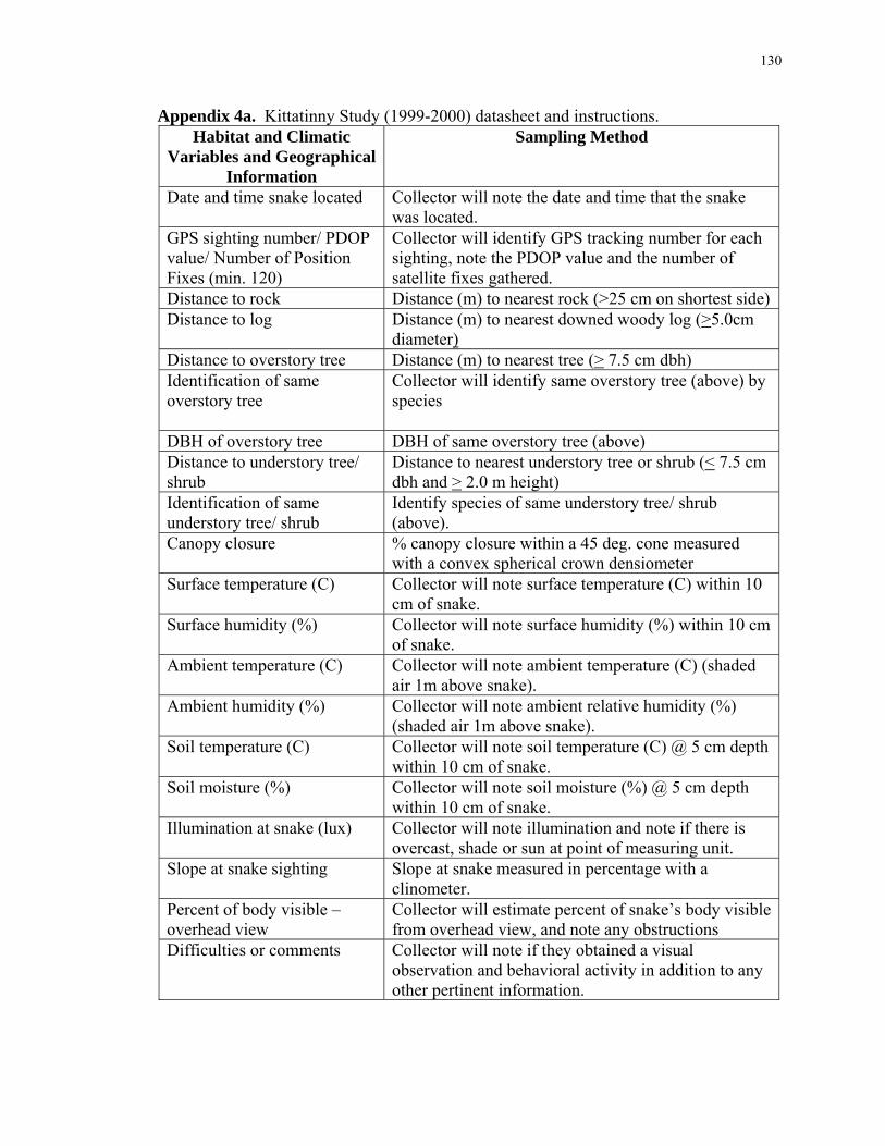
130
Appendix 4a. Kittatinny Study (1999-2000) datasheet and instructions.
Habitat and Climatic Variables and Geographical
Information
Sampling Method
Date and time snake located Collector will note the date and time that the snake was located.
GPS sighting number/ PDOP value/ Number of Position Fixes (min. 120)
Collector will identify GPS tracking number for each sighting, note the PDOP value and the number of satellite fixes gathered.
Distance to rock Distance (m) to nearest rock (>25 cm on shortest side) Distance to log Distance (m) to nearest downed woody log (>5.0cm
diameter) Distance to overstory tree Distance (m) to nearest tree (> 7.5 cm dbh) Identification of same overstory tree
Collector will identify same overstory tree (above) by species
DBH of overstory tree DBH of same overstory tree (above) Distance to understory tree/ shrub
Distance to nearest understory tree or shrub (< 7.5 cm dbh and > 2.0 m height)
Identification of same understory tree/ shrub
Identify species of same understory tree/ shrub (above).
Canopy closure % canopy closure within a 45 deg. cone measured with a convex spherical crown densiometer
Surface temperature (C)
Collector will note surface temperature (C) within 10 cm of snake.
Surface humidity (%)
Collector will note surface humidity (%) within 10 cm of snake.
Ambient temperature (C)
Collector will note ambient temperature (C) (shaded air 1m above snake).
Ambient humidity (%)
Collector will note ambient relative humidity (%) (shaded air 1m above snake).
Soil temperature (C)
Collector will note soil temperature (C) @ 5 cm depth within 10 cm of snake.
Soil moisture (%)
Collector will note soil moisture (%) @ 5 cm depth within 10 cm of snake.
Illumination at snake (lux) Collector will note illumination and note if there is overcast, shade or sun at point of measuring unit.
Slope at snake sighting Slope at snake measured in percentage with a clinometer.
Percent of body visible – overhead view
Collector will estimate percent of snake’s body visible from overhead view, and note any obstructions
Difficulties or comments Collector will note if they obtained a visual observation and behavioral activity in addition to any other pertinent information.
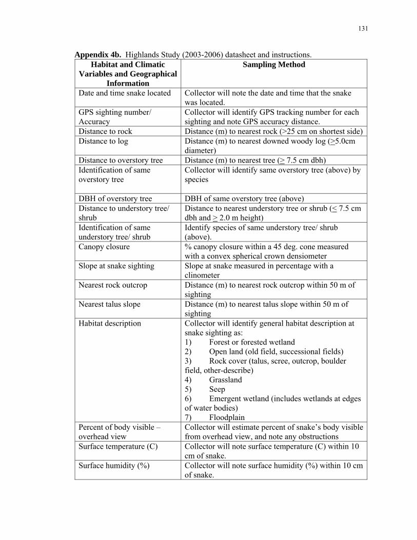
131
Appendix 4b. Highlands Study (2003-2006) datasheet and instructions.
Habitat and Climatic Variables and Geographical
Information
Sampling Method
Date and time snake located Collector will note the date and time that the snake was located.
GPS sighting number/ Accuracy
Collector will identify GPS tracking number for each sighting and note GPS accuracy distance.
Distance to rock Distance (m) to nearest rock (>25 cm on shortest side) Distance to log Distance (m) to nearest downed woody log (>5.0cm
diameter) Distance to overstory tree Distance (m) to nearest tree (> 7.5 cm dbh) Identification of same overstory tree
Collector will identify same overstory tree (above) by species
DBH of overstory tree DBH of same overstory tree (above) Distance to understory tree/ shrub
Distance to nearest understory tree or shrub (< 7.5 cm dbh and > 2.0 m height)
Identification of same understory tree/ shrub
Identify species of same understory tree/ shrub (above).
Canopy closure % canopy closure within a 45 deg. cone measured with a convex spherical crown densiometer
Slope at snake sighting Slope at snake measured in percentage with a clinometer
Nearest rock outcrop Distance (m) to nearest rock outcrop within 50 m of sighting
Nearest talus slope Distance (m) to nearest talus slope within 50 m of sighting
Habitat description Collector will identify general habitat description at snake sighting as: 1) Forest or forested wetland 2) Open land (old field, successional fields) 3) Rock cover (talus, scree, outcrop, boulder field, other-describe) 4) Grassland 5) Seep 6) Emergent wetland (includes wetlands at edges of water bodies) 7) Floodplain
Percent of body visible – overhead view
Collector will estimate percent of snake’s body visible from overhead view, and note any obstructions
Surface temperature (C)
Collector will note surface temperature (C) within 10 cm of snake.
Surface humidity (%)
Collector will note surface humidity (%) within 10 cm of snake.

132
Appendix 4b, continued.
Ambient temperature (C)
Collector will note ambient temperature (C) (shaded air 1m above snake).
Ambient humidity (%)
Collector will note ambient relative humidity (%) (shaded air 1m above snake).
Snake’s behavioral activity at sighting
A. Collector will note activity of snake as: 1) Hunting: active ambush, passive ambush, Reinert
position, scent trailing prey 2) Eating or drinking 3) Mating: copulation, courtship 4) Basking (collector will draw snake’s position):
alone, near/ with another snake 5) Traveling 6) Pre-shed, shedding 7) Within crevice: Partially or completely? Coiled
or stretched? B. Collector will note snake’s response to collector’s
presence 1) Silent: Still/ held ground OR moved away 2) Rattle: Rattle and hold ground OR rattle and
move away 3) Enlarges body in self defense 4) Continues activity without apparent disruption
General description of weather conditions
Collector will note general weather conditions at time of observation and if applicable, prior to observation (i.e. a rainy am will create high humidity in pm).
Note: Size and color phase of snake will be collected when snakes are collected for transmitter implantation.
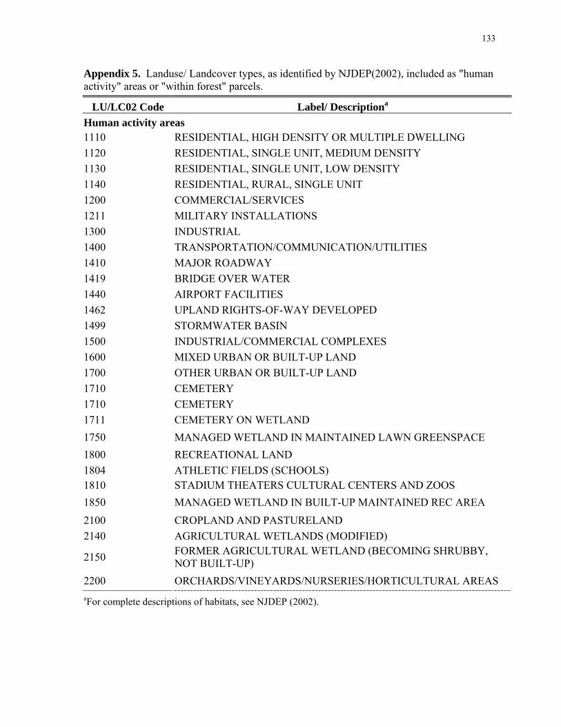
133
Appendix 5. Landuse/ Landcover types, as identified by NJDEP(2002), included as "human activity" areas or "within forest" parcels.
LU/LC02 Code Label/ Descriptiona Human activity areas 1110 RESIDENTIAL, HIGH DENSITY OR MULTIPLE DWELLING 1120 RESIDENTIAL, SINGLE UNIT, MEDIUM DENSITY 1130 RESIDENTIAL, SINGLE UNIT, LOW DENSITY 1140 RESIDENTIAL, RURAL, SINGLE UNIT 1200 COMMERCIAL/SERVICES 1211 MILITARY INSTALLATIONS 1300 INDUSTRIAL 1400 TRANSPORTATION/COMMUNICATION/UTILITIES 1410 MAJOR ROADWAY 1419 BRIDGE OVER WATER 1440 AIRPORT FACILITIES 1462 UPLAND RIGHTS-OF-WAY DEVELOPED 1499 STORMWATER BASIN 1500 INDUSTRIAL/COMMERCIAL COMPLEXES 1600 MIXED URBAN OR BUILT-UP LAND 1700 OTHER URBAN OR BUILT-UP LAND 1710 CEMETERY 1710 CEMETERY 1711 CEMETERY ON WETLAND 1750 MANAGED WETLAND IN MAINTAINED LAWN GREENSPACE 1800 RECREATIONAL LAND 1804 ATHLETIC FIELDS (SCHOOLS) 1810 STADIUM THEATERS CULTURAL CENTERS AND ZOOS 1850 MANAGED WETLAND IN BUILT-UP MAINTAINED REC AREA 2100 CROPLAND AND PASTURELAND 2140 AGRICULTURAL WETLANDS (MODIFIED)
2150 FORMER AGRICULTURAL WETLAND (BECOMING SHRUBBY, NOT BUILT-UP)
2200 ORCHARDS/VINEYARDS/NURSERIES/HORTICULTURAL AREAS aFor complete descriptions of habitats, see NJDEP (2002).

134
Appendix 5, continued. LU/LC02 Code Label/ Descriptiona
2300 CONFINED FEEDING OPERATIONS 2400 OTHER AGRICULTURE 5410 TIDAL RIVERS, INLAND BAYS, AND OTHER TIDAL WATERS 5420 DREDGED LAGOON 6111 SALINE MARSH (LOW MARSH) 6112 SALINE MARSH (HIGH MARSH) 6141 PHRAGMITES DOMINATE COASTAL WETLANDS 7100 BEACHES 7300 EXTRACTIVE MINING 7400 ALTERED LANDS 7500 TRANSITIONAL AREAS Forest habitats 4120 DECIDUOUS FOREST (>50% CROWN CLOSURE) 4220 CONIFEROUS FOREST (>50% CROWN CLOSURE)
4312 MIXED FOREST (>50% CONIFEROUS WITH >50% CROWN CLOSURE)
4322 MIXED FOREST (>50% DECIDUOUS WITH >50% CROWN CLOSURE)
6210 DECIDUOUS WOODED WETLANDS 6220 CONIFEROUS WOODED WETLANDS 6221 ATLANTIC WHITE CEDAR WETLANDS 6251 MIXED WOODED WETLANDS (DECIDUOUS DOM.) 6252 MIXED WOODED WETLANDS (CONIFEROUS DOM.) aFor complete descriptions of habitats, see NJDEP (2002).

135
Appendix 6a. Quantile plots (Q-Q plots) of microhabitat data collected at both snake-used and random (available) locations demonstrate the data does not have a normal distribution.

136
Appendix 6a, continued.

137
Appendix 6a, continued.

138
Appendix 6a, continued.

139
Appendix 6a, continued.

140
Appendix 6b. Quantile plots (Q-Q plots) of macrohabitat data collected at both snake-used and random (available) locations demonstrate the data does not have a normal distribution.

141
Appendix 6b, continued.
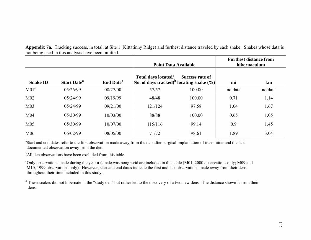
142
Appendix 7a. Tracking success, in total, at Site 1 (Kittatinny Ridge) and furthest distance traveled by each snake. Snakes whose data is not being used in this analysis have been omitted.
Point Data Available Furthest distance from
hibernaculum
Snake ID Start Datea End Datea Total days located/
No. of days tracked)bSuccess rate of
locating snake (%) mi km M01c 05/26/99 08/27/00 57/57 100.00 no data no data
M02 05/24/99 09/19/99 48/48 100.00 0.71 1.14
M03 05/24/99 09/21/00 121/124 97.58 1.04 1.67
M04 05/30/99 10/03/00 88/88 100.00 0.65 1.05
M05 05/30/99 10/07/00 115/116 99.14 0.9 1.45
M06 06/02/99 08/05/00 71/72 98.61 1.89 3.04 aStart and end dates refer to the first observation made away from the den after surgical implantation of transmitter and the last documented observation away from the den. bAll den observations have been excluded from this table. cOnly observations made during the year a female was nongravid are included in this table (M01, 2000 observations only; M09 and M10, 1999 observations only). However, start and end dates indicate the first and last observations made away from their dens throughout their time included in this study.
d These snakes did not hibernate in the "study den" but rather led to the discovery of a two new dens. The distance shown is from their dens.

143
Appendix 7a, continued.
Point Data Available Furthest distance from hibernaculum
Snake ID Start Datea End Datea
Total days located/ No. of days tracked)b
Success rate of locating snake (%) mi km
M07 07/20/99 09/21/00 98/98 100.00 1.60d 2.57
M08 07/22/99 09/27/00 84/85 98.82 1.15 1.85
M09c 08/18/99 09/29/00 21/21 100.00 0.48 0.77
M10c 08/28/99 09/24/00 15/15 100.00 1.08 1.74
M11 08/05/99 10/11/99 19/19 100.00 no data no data
M17 07/20/00 10/19/00 37/37 100.00 no data no data
TOTALS 774/780 99.23 - - aStart and end dates refer to the first observation made away from the den after surgical implantation of transmitter and the last documented observation away from the den. bAll den observations have been excluded from this table. cOnly observations made during the year a female was nongravid are included in this table (M01, 2000 observations only; M09 and M10, 1999 observations only). However, start and end dates indicate the first and last observations made away from their dens throughout their time included in this study. dThese snakes did not hibernate in the "study den" but rather led to the discovery of a two new dens. The distance shown is from their dens.
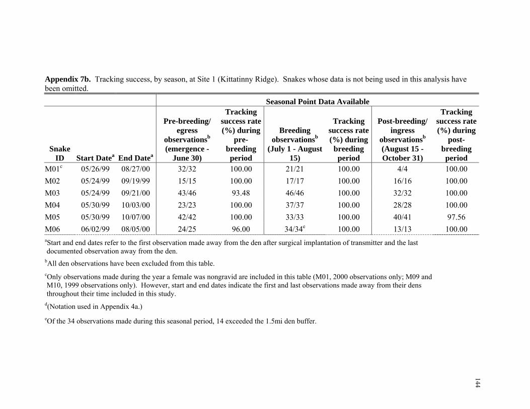
144
Appendix 7b. Tracking success, by season, at Site 1 (Kittatinny Ridge). Snakes whose data is not being used in this analysis have been omitted.
Seasonal Point Data Available
Snake ID Start Datea End Datea
Pre-breeding/ egress
observationsb (emergence -
June 30)
Tracking success rate (%) during
pre-breeding period
Breeding observationsb
(July 1 - August 15)
Tracking success rate (%) during
breeding period
Post-breeding/ ingress
observationsb (August 15 - October 31)
Tracking success rate (%) during
post-breeding period
M01c 05/26/99 08/27/00 32/32 100.00 21/21 100.00 4/4 100.00 M02 05/24/99 09/19/99 15/15 100.00 17/17 100.00 16/16 100.00 M03 05/24/99 09/21/00 43/46 93.48 46/46 100.00 32/32 100.00 M04 05/30/99 10/03/00 23/23 100.00 37/37 100.00 28/28 100.00 M05 05/30/99 10/07/00 42/42 100.00 33/33 100.00 40/41 97.56 M06 06/02/99 08/05/00 24/25 96.00 34/34e 100.00 13/13 100.00 aStart and end dates refer to the first observation made away from the den after surgical implantation of transmitter and the last documented observation away from the den. bAll den observations have been excluded from this table. cOnly observations made during the year a female was nongravid are included in this table (M01, 2000 observations only; M09 and M10, 1999 observations only). However, start and end dates indicate the first and last observations made away from their dens throughout their time included in this study. d(Notation used in Appendix 4a.) eOf the 34 observations made during this seasonal period, 14 exceeded the 1.5mi den buffer.

145
Appendix 7b, continued.
Snake ID Start Datea End Datea
Pre-breeding/ egress
observations (emergence -
June 30)
Tracking success rate (%) during
pre-breeding period
Breeding observations
(July 1 - August 15)
Tracking success rate (%) during
breeding period
Post-breeding/ ingress
observations (August 15 - October 31)
Tracking success rate (%) during
post-breeding period
M07 07/20/99 09/21/00 29/29 100.00 36/36 100.00 33/33 100.00 M08 07/22/99 09/27/00 21/21 100.00 33/33 100.00 30/31 96.77 M09c 08/18/99 09/29/00 0/0 n/a 0/0 n/a 21/21 100.00 M10c 08/28/99 09/24/00 0/0 n/a 0/0 n/a 15/15 100.00 M11 08/05/99 10/11/99 0/0 n/a 0/0 n/a 19/19 100.00 M17 07/20/00 10/19/00 0/0 n/a 14/14 100.00 23/23 100.00
TOTALS 229/233 98.28 271/271 100.00 274/276 99.28 aStart and end dates refer to the first observation made away from the den after surgical implantation of transmitter and the last documented observation away from the den. bAll den observations have been excluded from this table. cOnly observations made during the year a female was nongravid are included in this table (M01, 2000 observations only; M09 and M10, 1999 observations only). However, start and end dates indicate the first and last observations made away from their dens throughout their time included in this study. d(Notation used in Appendix 4a.)
eOf the 34 observations made during this seasonal period, 14 exceeded the 1.5mi den buffer.

146
Appendix 8a. Tracking success, in total, at Site 2 (Highlands Region) and furthest distance traveled by each snake. Snakes whose data is not being used in this analysis have been omitted.
Total point data available Furthest recorded distance from
hibernaculum
Snake ID Start Datea End Datea
Total days located/ No. of days tracked)b
Success rate of locating snake (%) mi km
H01 06/10/03 10/04/03 28/29 96.55 1.24 2.00
H02 06/10/03 06/15/04 42/47 89.36 1.71 2.75
H03 06/06/03 10/04/03 32/32 100.00 0.97 1.56
H10 07/13/03 08/13/03 12/12 100.00 0.68 1.09
H16c 07/28/03 06/04/04 26/26 100.00 0.91 1.46
H18 10/22/03 08/12/04 41/42 97.62 0.74 1.19
H20 07/09/04 07/24/05 73/75 97.33 0.86 1.38
H21 07/17/04 07/30/05 83/86 96.51 2.13 3.43
H22 07/25/04 08/07/05 58/62 93.55 1.66 2.67
H23 07/17/04 05/31/05 10/13 76.92 0.79 1.27 aStart and end dates refer to the first observation made away from the den after surgical implantation of transmitter and the last documented observation away from the den. bAll den observations have been excluded from this table. cSnake H16 was incorporated into study in late July 2003 and tracked until mid-August but then not tracked again until the denning period in late October. H16 was tracked into early July but then removed from study due to anticipated transmitter failure.

147
Appendix 8a, continued.
Total point data available Furthest recorded distance from
hibernaculum
Snake ID Start Datea End Datea
Total days located/ No. of days tracked)b
Success rate of locating snake (%) mi km
H24 07/21/04 06/04/05 16/16 100.00 0.71 1.14
H26 08/07/04 10/06/05 71/74 95.95 1.85 2.98
H27 08/18/04 08/03/05 67/67 100.00 1.77 2.85
H28 08/26/04 08/01/05 62/62 100.00 2.28 3.67
H29 08/15/04 05/15/05 31/31 100.00 0.75 1.21
TOTALS 652/674 96.74 aStart and end dates refer to the first observation made away from the den after surgical implantation of transmitter and the last documented observation away from the den. bAll den observations have been excluded from this table. cSnake H16 was incorporated into study in late July 2003 and tracked until mid-August but then not tracked again until the denning period in late October. H16 was tracked into early July but then removed from study due to anticipated transmitter failure.

148
Appendix 8b. Tracking success, by season, at Site 2 (Highlands Region). Snakes whose data is not being used in this analysis have been omitted.
Seasonal point data available
Snake ID Start Datea End Datea
Pre-breeding observations
(May - June 30)
Tracking success rate (%) during
pre-breeding period
Breeding observations
(July 1 - August 15)
Tracking success rate (%) during
breeding period
Post-breeding/ Ingress
observations (August 15 - October 31)
Tracking success rate (%) during
post-breeding period
H01 06/10/03 10/04/03 5/6 83.33 21/21 100.00 2/2 100.00
H02 06/10/03 06/15/04 25/27d 92.59 17/20d 85.00 0/0 0.00
H03 06/06/03 10/04/03 6/6 100.00 23/23 100.00 3/3e 100.00
H10 07/13/03 08/13/03 0/0 n/a 12/12 100.00 0/0 n/a
H16c 07/28/03 06/04/04 17/17 100.00 7/7 100.00 2/2 100.00 aStart and end dates refer to the first observation made away from the den after surgical implantation of transmitter and the last documented observation away from the den. bAll den observations have been excluded from this table. cSnake H16 was incorporated into study in late July 2003 and tracked until mid-August but then not tracked again until the denning period in late October. H16 was tracked into early July but then removed from study due to anticipated transmitter failure. dSome observations were outside of the snake's 1.5mi den buffer. eTransmitters had unscheduled failures. H03's transmitter failed during hibernation and H23 and H29's transmitters failed early in the 2005 season and were not recovered.

149
Appendix 8b, continued.
Snake ID Start Datea End Datea
Pre-breeding observations (May - June
30)
Tracking success rate (%) during
pre-breeding period
Breeding observations
(July 1 - August 15)
Tracking success rate (%) during
breeding period
Post-breeding/ Ingress
observations (August 15 - October 31)
Tracking success rate (%) during
post-breeding period
H18 10/22/03 08/12/04 28/28 100.00 12/13 92.31 1/1 100.00
H20 07/09/04 07/24/05 26/26 100.00 28/30 93.33 19/19 100.00
H21 07/17/04 07/30/05 28/28 100.00 28/31 90.32 27/27 100.00
H22 07/25/04 08/07/05 29/29 100.00 21/25d 84.00 8/8 100.00
H23 07/17/04 05/31/05 7/10e 70.00 1/1 100.00 2/2 100.00
H24 07/21/04 06/04/05 15/15 100.00 1/1 100.00 0/0 n/a aStart and end dates refer to the first observation made away from the den after surgical implantation of transmitter and the last documented observation away from the den. bAll den observations have been excluded from this table. cSnake H16 was incorporated into study in late July 2003 and tracked until mid-August but then not tracked again until the denning period in late October. H16 was tracked into early July but then removed from study due to anticipated transmitter failure. dSome observations were outside of the snake's 1.5mi den buffer. eTransmitters had unscheduled failures. H03's transmitter failed during hibernation and H23 and H29's transmitters failed early in the 2005 season and were not recovered.

150
Appendix 8b, continued.
Snake ID Start Datea End Datea
Pre-breeding observations (May - June
30)
Tracking success rate (%) during
pre-breeding period
Breeding observations
(July 1 - August 15)
Tracking success rate (%) during
breeding period
Post-breeding/ Ingress
observations (August 15 - October 31)
Tracking success rate (%) during
post-breeding period
H26 08/07/04 10/06/05 25/28 89.29 21/21d 100.00 25/25 100.00
H27 08/18/04 08/03/05 25/25 100.00 16/16 100.00 26/26 100.00
H28 08/26/04 08/01/05 27/27 100.00 15/15 100.00 20/20d 100.00
H29 08/15/04 05/15/05 6/6e 100.00 1/1 100.00 24/24 100.00
TOTALS 269/278 96.76 224/237 94.51 159/159 100.00 aStart and end dates refer to the first observation made away from the den after surgical implantation of transmitter and the last documented observation away from the den. bAll den observations have been excluded from this table. cSnake H16 was incorporated into study in late July 2003 and tracked until mid-August but then not tracked again until the denning period in late October. H16 was tracked into early July but then removed from study due to anticipated transmitter failure. dSome observations were outside of the snake's 1.5mi den buffer. eTransmitters had unscheduled failures. H03's transmitter failed during hibernation and H23 and H29's transmitters failed early in the 2005 season and were not recovered.

151
Appendix 9a. Sample sizes per study site and microhabitat variable collected at random habitats and snakes' stationary observations (males and females), excluding observations at repeated locations and dens.
Distance to rock
Distance to log
Distance to
overstory tree
DBH of overstory
tree
Distance to understory tree/shrub Canopy Slope
Distance to rock outcrop
(w/i 50m)
Distance to talus
(w/i 50m)
Site 1 (Kittatinny) Snakes; n = 429 433 430 430 432 431 224 n/a n/a Site 1 (Kittatinny) Random; n = 94 94 94 94 94 93 1 n/a n/a
Site 2 (Highlands) Snakes; n = 370 368 370 362 369 369 321 321 322 Site 2 (Highlands) Random; n = 251 251 251 251 251 246 249 249 250
Snakes; n = 799 801 800 792 801 800 545 321 322 TOTALS
Random; n = 345 345 345 345 345 339 250 249 250
Appendix 9b. Sample sizes per study site and macrohabitat variable collected at random habitats and snakes' stationary observations (males and females), excluding observations at repeated locations and dens.
Proximity to
streams/rivers Proximity to human
activity Proximity to forest
edge Proximity to roadsSite 1 (Kittatinny) Snakes; n = 191 191 191 191 Site 1 (Kittatinny) Random; n = 1,793 1,793 1,793 1,793
Site 2 (Highlands) Snakes; n = 358 358 358 358 Site 2 (Highlands) Random; n = 10,799 10,799 10,799 10,799
Snakes; n = 549 549 549 549 TOTALS
Random; n = 12,592 12,592 12,592 12,592

152
Appendix 10. Proportional comparison of expected and actual use of the available habitat as identified by NJDEP, LU/LC02 (2002) by transmitter-implanted timber rattlesnakes. LU/LC02 types are in order of snake use.
LU/LC02 ID and Labela
Acres of LULC
within den bufferb
Snake(s) associated
with the den
Relative acreage per den buffer
Expected # of obs.
All stationary
obs.
2435.03 H01, H02 0.740 33.31 40
2212.52 H23 0.492 4.92 6
2295.65 H24 0.510 7.65 14
3736.05 H16 0.830 13.28 18
3734.25 H03 0.830 24.06 21
3667.49 H21, H27 0.815 109.19 120
3904.73 H22, H28 0.868 84.15 79
3491.25 H26 0.776 45.76 47
H20 (♂) 1220.36
H29 (♀) 0.271 25.22 40
1629.86 H18 0.362 14.85 23
1430.87 H10 0.318 3.81 10
4120
DEC
IDU
OU
S FO
RES
T (>
50%
CR
OW
N C
LOSU
RE)
M02, M03, M04, M05, M06 (♂)
2696.86
M09 (♀)
0.599 118.64 133
TOTALS 32454.92 7.41 484.84 551
aLULC02 code and Label are identified and described in further detail by NJDEP, 2002. bAcreages were summed per LU/LC02 within each den buffer regardless of overlap. NOTE: Two dens are based on four den buffers.

153
Appendix 10, continued.
LU/LC02 ID and Labela
Acres of LULC
within den bufferb
Snake(s) associated
with the den
Relative acreage per den buffer
Expected # of obs.
All stationary
obs.
26.37 H01, H02 0.008 0.36 0
103.64 H23 0.023 0.23 0
133.11 H24 0.030 0.44 0
161.08 H16 0.036 0.57 0
161.01 H03 0.036 1.04 0
159.15 H21, H27 0.035 4.74 8
99.76 H22, H28 0.022 2.15 2
152.29 H26 0.034 2.00 0
H20 (♂) 287.24
H29 (♀) 0.064 5.93 41
53.22 H18 0.012 0.48 0
293.36 H10 0.065 0.78 1
M02, M03, M04, M05, M06 (♂)
4110
DEC
IDU
OU
S FO
RES
T (1
0-50
% C
RO
WN
CLO
SUR
E)
210.51
M09 (♀)
0.047 9.26 39
TOTALS 1840.73 0.41 27.99 91 aLULC02 code and Label are identified and described in further detail by NJDEP, 2002. bAcreages were summed per LU/LC02 within each den buffer regardless of overlap. NOTE: Two dens are based on four den buffers.

154
Appendix 10, continued.
LU/LC02 ID and Labela
Acres of LULC
within den bufferb
Snake(s) associated
with the den
Relative acreage per den buffer
Expected # of obs.
All stationary
obs.
132.83 H01, H02 0.040 1.82 5
281.36 H23 0.063 0.63 1
261.15 H24 0.058 0.87 0
273.09 H16 0.061 0.97 0
272.35 H03 0.061 1.75 0
260.65 H21, H27 0.058 7.76 5
274.54 H22, H28 0.061 5.92 6
174.23 H26 0.039 2.28 0
H20 (♂) 231.54
H29 (♀) 0.051 4.78 0
140.62 H18 0.031 1.28 16
217.35 H10 0.048 0.58 0
6210
DEC
IDU
OU
S W
OO
DED
WET
LAN
DS
M02, M03, M04, M05, M06 (♂)
162.52
M09 (♀)
0.036 7.15 2
TOTALS 2682.23 0.61 35.79 35 aLULC02 code and Label are identified and described in further detail by NJDEP, 2002. bAcreages were summed per LU/LC02 within each den buffer regardless of overlap. NOTE: Two dens are based on four den buffers.
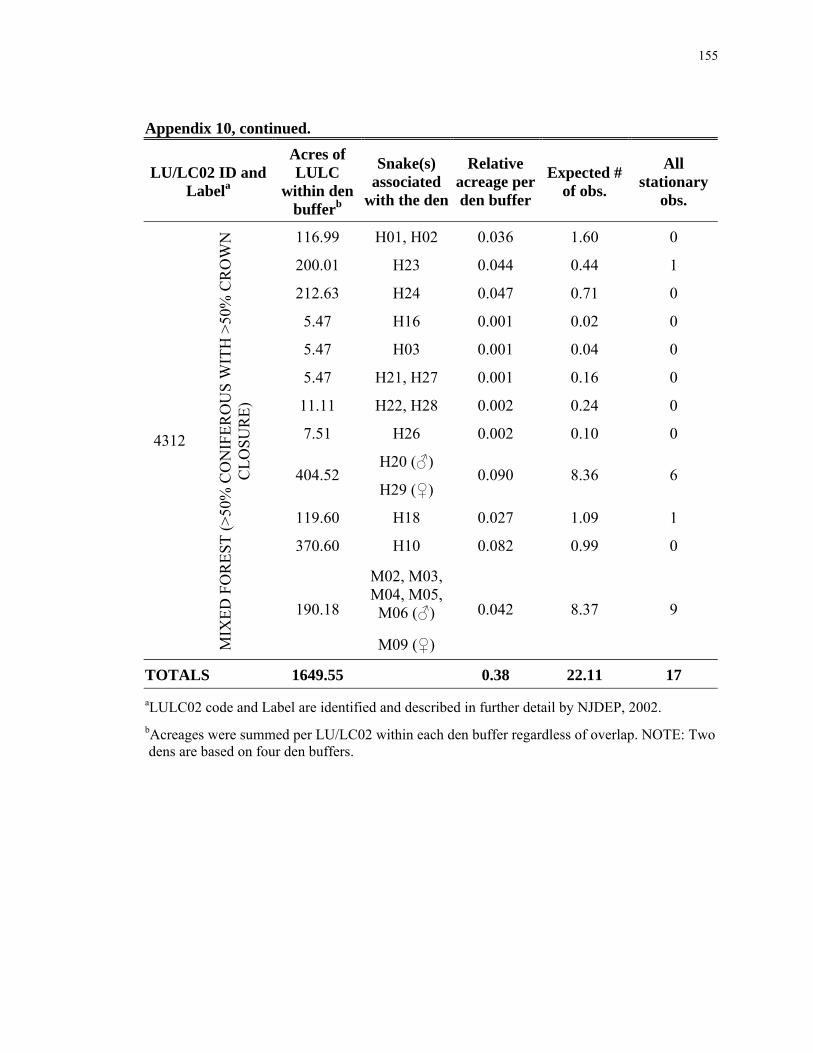
155
Appendix 10, continued.
LU/LC02 ID and Labela
Acres of LULC
within den bufferb
Snake(s) associated
with the den
Relative acreage per den buffer
Expected # of obs.
All stationary
obs.
116.99 H01, H02 0.036 1.60 0
200.01 H23 0.044 0.44 1
212.63 H24 0.047 0.71 0
5.47 H16 0.001 0.02 0
5.47 H03 0.001 0.04 0
5.47 H21, H27 0.001 0.16 0
11.11 H22, H28 0.002 0.24 0
7.51 H26 0.002 0.10 0
H20 (♂) 404.52
H29 (♀) 0.090 8.36 6
119.60 H18 0.027 1.09 1
370.60 H10 0.082 0.99 0
M02, M03, M04, M05, M06 (♂)
4312
MIX
ED F
OR
EST
(>50
% C
ON
IFER
OU
S W
ITH
>50
% C
RO
WN
C
LOSU
RE)
190.18
M09 (♀)
0.042 8.37 9
TOTALS 1649.55 0.38 22.11 17 aLULC02 code and Label are identified and described in further detail by NJDEP, 2002. bAcreages were summed per LU/LC02 within each den buffer regardless of overlap. NOTE: Two dens are based on four den buffers.

156
Appendix 10, continued.
LU/LC02 ID and Labela
Acres of LULC
within den bufferb
Snake(s) associated
with the den
Relative acreage per den buffer
Expected # of obs.
All stationary
obs.
1.34 H01, H02 0.000 0.02 0 H20 (♂)
17.68 H29 (♀)
0.004 0.37 0
60.52 H18 0.013 0.55 0 13.23 H10 0.003 0.04 0
M02, M03, M04, M05, M06 (♂)
4440
MIX
ED D
ECID
UO
US/
C
ON
IFER
OU
S B
RU
SH/
SHR
UB
LAN
D
37.05
M09 (♀)
0.008 1.63 10
TOTALS 129.81 0.03 2.60 10 4.33 H01, H02 0.001 0.06 0 1.05 H23 0.000 0.00 0 1.05 H24 0.000 0.00 0 2.01 H16 0.000 0.01 0 0.86 H03 0.000 0.01 0 5.77 H22, H28 0.001 0.12 10 0.11 H26 0.000 0.00 0
H20 (♂) 16.12
H29 (♀) 0.004 0.33 0
28.22 H18 0.006 0.26 0 9.81 H10 0.002 0.03 0
M02, M03, M04, M05, M06 (♂)
4420
DEC
IDU
OU
S B
RU
SH/ S
HR
UB
LAN
D
18.36
M09 (♀)
0.004 0.81 0
TOTALS 87.70 0.02 1.63 10 aLULC02 code and Label are identified and described in further detail by NJDEP, 2002. bAcreages were summed per LU/LC02 within each den buffer regardless of overlap. NOTE: Two dens are based on four den buffers.
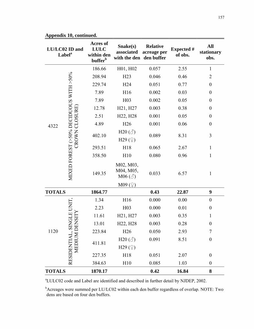
157
Appendix 10, continued.
LU/LC02 ID and Labela
Acres of LULC
within den bufferb
Snake(s) associated
with the den
Relative acreage per den buffer
Expected # of obs.
All stationary
obs.
186.66 H01, H02 0.057 2.55 1 208.94 H23 0.046 0.46 2 229.74 H24 0.051 0.77 0 7.89 H16 0.002 0.03 0 7.89 H03 0.002 0.05 0 12.78 H21, H27 0.003 0.38 0 2.51 H22, H28 0.001 0.05 0 4.89 H26 0.001 0.06 0
H20 (♂) 402.10
H29 (♀) 0.089 8.31 3
293.51 H18 0.065 2.67 1 358.50 H10 0.080 0.96 1
M02, M03, M04, M05, M06 (♂)
4322
MIX
ED F
OR
EST
(>50
% D
ECID
UO
US
WIT
H >
50%
C
RO
WN
CLO
SUR
E)
149.35
M09 (♀)
0.033 6.57 1
TOTALS 1864.77 0.43 22.87 9 1.34 H16 0.000 0.00 0 2.23 H03 0.000 0.01 0 11.61 H21, H27 0.003 0.35 1 13.01 H22, H28 0.003 0.28 0 223.84 H26 0.050 2.93 7
H20 (♂) 0.091 8.51 0 411.81
H29 (♀) 227.35 H18 0.051 2.07 0
1120
RES
IDEN
TIA
L, S
ING
LE U
NIT
, M
EDIU
M D
ENSI
TY
384.63 H10 0.085 1.03 0 TOTALS 1870.17 0.42 16.84 8 aLULC02 code and Label are identified and described in further detail by NJDEP, 2002. bAcreages were summed per LU/LC02 within each den buffer regardless of overlap. NOTE: Two dens are based on four den buffers.
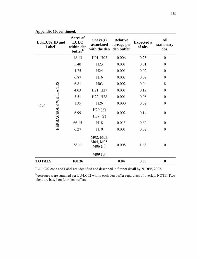
158
Appendix 10, continued.
LU/LC02 ID and Labela
Acres of LULC
within den bufferb
Snake(s) associated
with the den
Relative acreage per den buffer
Expected # of obs.
All stationary
obs.
18.13 H01, H02 0.006 0.25 0
5.40 H23 0.001 0.01 0
4.75 H24 0.001 0.02 0
6.87 H16 0.002 0.02 0
6.81 H03 0.002 0.04 8
4.03 H21, H27 0.001 0.12 0
3.51 H22, H28 0.001 0.08 0
1.35 H26 0.000 0.02 0
H20 (♂) 6.99
H29 (♀) 0.002 0.14 0
66.15 H18 0.015 0.60 0
6.27 H10 0.001 0.02 0
M02, M03, M04, M05, M06 (♂)
6240
HER
BA
CEO
US
WET
LAN
DS
38.11
M09 (♀)
0.008 1.68 0
TOTALS 168.36 0.04 3.00 8 aLULC02 code and Label are identified and described in further detail by NJDEP, 2002. bAcreages were summed per LU/LC02 within each den buffer regardless of overlap. NOTE: Two dens are based on four den buffers.

159
Appendix 10, continued.
LU/LC02 ID and Labela
Acres of LULC
within den bufferb
Snake(s) associated
with the den
Relative acreage per den buffer
Expected # of obs.
All stationary
obs.
19.21 H23 0.004 0.04 0
27.64 H24 0.006 0.09 0
31.89 H16 0.007 0.11 1
31.98 H03 0.007 0.21 0
32.60 H21, H27 0.007 0.97 0
25.40 H22, H28 0.006 0.55 0
35.34 H26 0.008 0.46 5
H20 (♂) 18.88
H29 (♀) 0.004 0.39 0
26.87 H18 0.006 0.24 0
21.18 H10 0.005 0.06 0
M02, M03, M04, M05, M06 (♂)
1463
UPL
AN
D R
IGH
TS-O
F-W
AY
UN
DEV
ELO
PED
37.28
M09 (♀)
0.008 1.64 0
TOTALS 308.26 0.07 4.77 6 aLULC02 code and Label are identified and described in further detail by NJDEP, 2002. bAcreages were summed per LU/LC02 within each den buffer regardless of overlap. NOTE: Two dens are based on four den buffers.
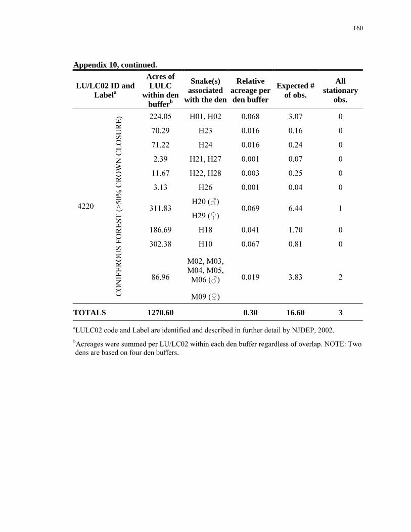
160
Appendix 10, continued.
LU/LC02 ID and Labela
Acres of LULC
within den bufferb
Snake(s) associated
with the den
Relative acreage per den buffer
Expected # of obs.
All stationary
obs.
224.05 H01, H02 0.068 3.07 0
70.29 H23 0.016 0.16 0
71.22 H24 0.016 0.24 0
2.39 H21, H27 0.001 0.07 0
11.67 H22, H28 0.003 0.25 0
3.13 H26 0.001 0.04 0
H20 (♂) 311.83
H29 (♀) 0.069 6.44 1
186.69 H18 0.041 1.70 0
302.38 H10 0.067 0.81 0
M02, M03, M04, M05, M06 (♂)
4220
CO
NIF
ERO
US
FOR
EST
(>50
% C
RO
WN
CLO
SUR
E)
86.96
M09 (♀)
0.019 3.83 2
TOTALS 1270.60 0.30 16.60 3
aLULC02 code and Label are identified and described in further detail by NJDEP, 2002. bAcreages were summed per LU/LC02 within each den buffer regardless of overlap. NOTE: Two dens are based on four den buffers.

161
Appendix 10, continued.
LU/LC02 ID and Labela
Acres of LULC
within den bufferb
Snake(s) associated
with the den
Relative acreage per den buffer
Expected # of obs.
All stationary
obs.
251.84 H23 0.056 0.56 0
202.49 H24 0.045 0.67 1
0.48 H16 0.000 0.00 0
1.73 H03 0.000 0.01 0
16.05 H21, H27 0.004 0.48 0
2.22 H22, H28 0.000 0.05 0
201.29 H26 0.045 2.64 0
H20 (♂) 128.15
H29 (♀) 0.028 2.65 1
73.07 H18 0.016 0.67 0
126.71 H10 0.028 0.34 0
M02, M03, M04, M05, M06 (♂)
1130
RES
IDEN
TIA
L, S
ING
LE U
NIT
, LO
W D
ENSI
TY
35.06
M09 (♀)
0.008 1.54 0
TOTALS 1039.08 0.23 9.60 2 aLULC02 code and Label are identified and described in further detail by NJDEP, 2002. bAcreages were summed per LU/LC02 within each den buffer regardless of overlap. NOTE: Two dens are based on four den buffers.
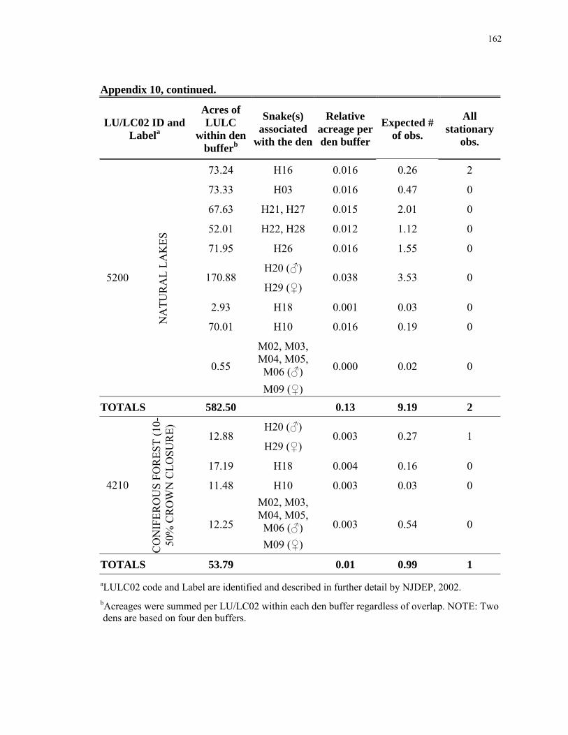
162
Appendix 10, continued.
LU/LC02 ID and Labela
Acres of LULC
within den bufferb
Snake(s) associated
with the den
Relative acreage per den buffer
Expected # of obs.
All stationary
obs.
73.24 H16 0.016 0.26 2
73.33 H03 0.016 0.47 0
67.63 H21, H27 0.015 2.01 0
52.01 H22, H28 0.012 1.12 0
71.95 H26 0.016 1.55 0
H20 (♂) 170.88
H29 (♀) 0.038 3.53 0
2.93 H18 0.001 0.03 0
70.01 H10 0.016 0.19 0
M02, M03, M04, M05, M06 (♂)
5200
NA
TUR
AL
LAK
ES
0.55
M09 (♀)
0.000 0.02 0
TOTALS 582.50 0.13 9.19 2
H20 (♂) 12.88
H29 (♀) 0.003 0.27 1
17.19 H18 0.004 0.16 0
11.48 H10 0.003 0.03 0 M02, M03, M04, M05, M06 (♂)
4210
CO
NIF
ERO
US
FOR
EST
(10-
50%
CR
OW
N C
LOSU
RE)
12.25
M09 (♀)
0.003 0.54 0
TOTALS 53.79 0.01 0.99 1 aLULC02 code and Label are identified and described in further detail by NJDEP, 2002. bAcreages were summed per LU/LC02 within each den buffer regardless of overlap. NOTE: Two dens are based on four den buffers.
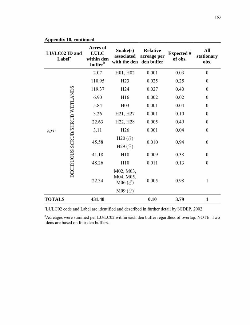
163
Appendix 10, continued.
LU/LC02 ID and Labela
Acres of LULC
within den bufferb
Snake(s) associated
with the den
Relative acreage per den buffer
Expected # of obs.
All stationary
obs.
2.07 H01, H02 0.001 0.03 0
110.95 H23 0.025 0.25 0
119.37 H24 0.027 0.40 0
6.90 H16 0.002 0.02 0
5.84 H03 0.001 0.04 0
3.26 H21, H27 0.001 0.10 0
22.63 H22, H28 0.005 0.49 0
3.11 H26 0.001 0.04 0
H20 (♂) 45.58
H29 (♀) 0.010 0.94 0
41.18 H18 0.009 0.38 0
48.26 H10 0.011 0.13 0
M02, M03, M04, M05, M06 (♂)
6231
DEC
IDU
OU
S SC
RU
B/S
HR
UB
WET
LAN
DS
22.34
M09 (♀)
0.005 0.98 1
TOTALS 431.48 0.10 3.79 1 aLULC02 code and Label are identified and described in further detail by NJDEP, 2002. bAcreages were summed per LU/LC02 within each den buffer regardless of overlap. NOTE: Two dens are based on four den buffers.

164
Appendix 10, continued.
LU/LC02 ID and Labela
Acres of LULC
within den bufferb
Snake(s) associated
with the den
Relative acreage per den buffer
Expected # of obs.
All stationary
obs.
19.89 H01, H02 0.006 0.27 0
26.44 H23 0.006 0.06 0
31.50 H24 0.007 0.10 0
H20 (♂) 92.81
H29 (♀) 0.021 1.92 0
8.28 H18 0.002 0.08 0
65.49 H10 0.015 0.17 0
M02, M03, M04, M05, M06 (♂)
4321
MIX
ED F
OR
EST
(>50
% D
ECID
UO
US
WIT
H 1
0-50
% C
RO
WN
CLO
SUR
E)
45.16
M09 (♀)
0.010 1.99 1
TOTALS 289.58 0.07 4.59 1 aLULC02 code and Label are identified and described in further detail by NJDEP, 2002. bAcreages were summed per LU/LC02 within each den buffer regardless of overlap. NOTE: Two dens are based on four den buffers.

165
Appendix 10, continued.
LU/LC02 ID and Labela
Acres of LULC
within den bufferb
Snake(s) associated
with the den
Relative acreage per den buffer
Expected # of obs.
All stationary
obs.
13.04 H01, H02 0.004 0.18 1
8.36 H23 0.002 0.02 0
4.23 H24 0.001 0.01 0
8.49 H16 0.002 0.03 0
8.49 H03 0.002 0.05 0
8.74 H21, H27 0.002 0.26 0
1.09 H22, H28 0.000 0.02 0
3.05 H26 0.001 0.04 0
H20 (♂) 18.70
H29 (♀) 0.004 0.39 0
19.37 H18 0.004 0.18 0
17.86 H10 0.004 0.05 0
M02, M03, M04, M05, M06 (♂)
1700
OTH
ER U
RB
AN
OR
BU
ILT-
UP
LAN
D
11.40
M09 (♀)
0.008 1.63 0
TOTALS 122.81 0.03 2.86 1 aLULC02 code and Label are identified and described in further detail by NJDEP, 2002. bAcreages were summed per LU/LC02 within each den buffer regardless of overlap. NOTE: Two dens are based on four den buffers.
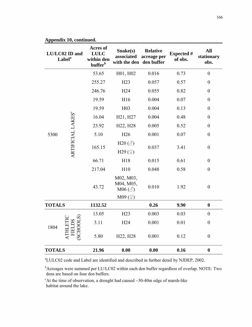
166
Appendix 10, continued.
LU/LC02 ID and Labela
Acres of LULC
within den bufferb
Snake(s) associated
with the den
Relative acreage per den buffer
Expected # of obs.
All stationary
obs.
53.65 H01, H02 0.016 0.73 0
255.27 H23 0.057 0.57 0
246.76 H24 0.055 0.82 0
19.59 H16 0.004 0.07 0
19.59 H03 0.004 0.13 0
16.04 H21, H27 0.004 0.48 0
23.92 H22, H28 0.005 0.52 0
5.10 H26 0.001 0.07 0
H20 (♂) 165.15
H29 (♀) 0.037 3.41 0
66.71 H18 0.015 0.61 0
217.04 H10 0.048 0.58 0
M02, M03, M04, M05, M06 (♂)
5300
AR
TIFI
CIA
L LA
KES
c
43.72
M09 (♀)
0.010 1.92 0
TOTALS 1132.52 0.26 9.90 0
13.05 H23 0.003 0.03 0
3.11 H24 0.001 0.01 0 1804
ATH
LETI
C
FIEL
DS
(SC
HO
OLS
)
5.80 H22, H28 0.001 0.12 0
TOTALS 21.96 0.00 0.00 0.16 0 aLULC02 code and Label are identified and described in further detail by NJDEP, 2002. bAcreages were summed per LU/LC02 within each den buffer regardless of overlap. NOTE: Two dens are based on four den buffers. cAt the time of observation, a drought had caused ~30-40m edge of marsh-like habitat around the lake.

167
Appendix 10, continued.
LU/LC02 ID and Labela
Acres of LULC
within den bufferb
Snake(s) associated
with the den
Relative acreage per den buffer
Expected # of obs.
All stationary
obs.
12.39 H23 0.003 0.03 0
3.84 H24 0.001 0.01 0
29.80 H16 0.007 0.11 0
30.02 H03 0.007 0.19 0
35.17 H21, H27 0.008 1.05 0
3.51 H22, H28 0.001 0.08 0
15.69 H26 0.003 0.21 0
H20 (♂) 40.38
H29 (♀) 0.009 0.83 0
574.85 H18 0.128 5.24 0
36.99 H10 0.008 0.10 0
M02, M03, M04, M05, M06 (♂)
2100
CR
OPL
AN
D A
ND
PA
STU
REL
AN
D
294.66
M09 (♀)
0.065 12.96 0
TOTALS 1077.29 0.24 20.80 0
2150
FOR
MER
AG
RIC
ULT
UR
AL
WET
LAN
D (B
ECO
MIN
G
SHR
UB
BY
, NO
T B
UIL
T-U
P)
55.98 H18 0.012 0.51 0
TOTALS 55.98 0.01 0.51 0
aLULC02 code and Label are identified and described in further detail by NJDEP, 2002. bAcreages were summed per LU/LC02 within each den buffer regardless of overlap. NOTE: Two dens are based on four den buffers.
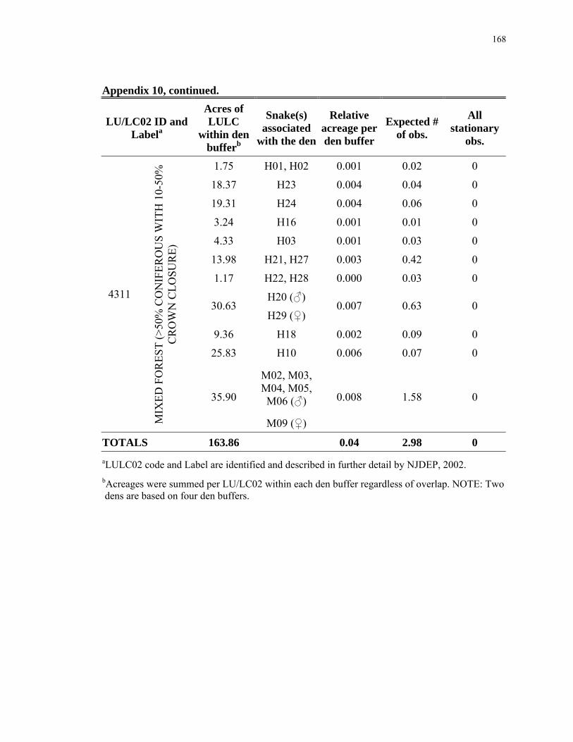
168
Appendix 10, continued.
LU/LC02 ID and Labela
Acres of LULC
within den bufferb
Snake(s) associated
with the den
Relative acreage per den buffer
Expected # of obs.
All stationary
obs.
1.75 H01, H02 0.001 0.02 0
18.37 H23 0.004 0.04 0
19.31 H24 0.004 0.06 0
3.24 H16 0.001 0.01 0
4.33 H03 0.001 0.03 0
13.98 H21, H27 0.003 0.42 0
1.17 H22, H28 0.000 0.03 0
H20 (♂) 30.63
H29 (♀) 0.007 0.63 0
9.36 H18 0.002 0.09 0
25.83 H10 0.006 0.07 0
M02, M03, M04, M05, M06 (♂)
4311
MIX
ED F
OR
EST
(>50
% C
ON
IFER
OU
S W
ITH
10-
50%
C
RO
WN
CLO
SUR
E)
35.90
M09 (♀)
0.008 1.58 0
TOTALS 163.86 0.04 2.98 0 aLULC02 code and Label are identified and described in further detail by NJDEP, 2002. bAcreages were summed per LU/LC02 within each den buffer regardless of overlap. NOTE: Two dens are based on four den buffers.

169
Appendix 10, continued.
LU/LC02 ID and Labela
Acres of LULC
within den bufferb
Snake(s) associated
with the den
Relative acreage per den buffer
Expected # of obs.
All stationary
obs.
2.00 H01, H02 0.001 0.03 0
1.19 H22, H28 0.000 0.03 0
H20 (♂) 10.70
H29 (♀) 0.002 0.22 0
88.51 H18 0.020 0.81 0 10.70 H10 0.002 0.03 0
M02, M03, M04, M05, M06 (♂)
4430
CO
NIF
ERO
US
BR
USH
/ SH
RU
BLA
ND
41.18
M09 (♀)
0.009 1.81 0
TOTALS 154.28 0.03 2.92 0
0.80 H01, H02 0.000 0.01 0
61.99 H23 0.014 0.14 0
49.16 H24 0.011 0.16 0
17.43 H16 0.004 0.06 0
17.43 H03 0.004 0.11 0
18.90 H21, H27 0.004 0.56 0
17.43 H22, H28 0.004 0.38 0
37.50 H26 0.008 0.49 0
H20 (♂) 41.48
H29 (♀) 0.009 0.86 0
37.39 H10 0.008 0.10 0
M02, M03, M04, M05, M06 (♂)
1800
REC
REA
TIO
NA
L LA
ND
9.50
M09 (♀)
0.002 0.42 0
TOTALS 309.00 0.07 3.29 0 aLULC02 code and Label are identified and described in further detail by NJDEP, 2002. bAcreages were summed per LU/LC02 within each den buffer regardless of overlap. NOTE: Two dens are based on four den buffers.
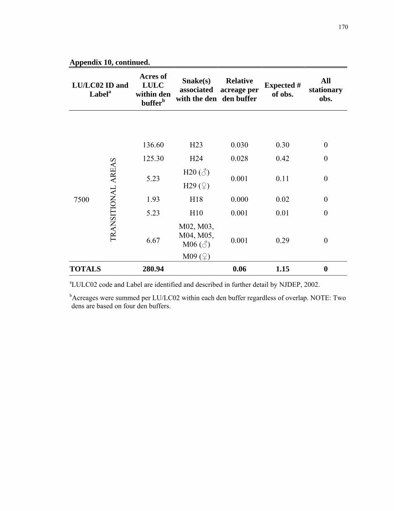
170
Appendix 10, continued.
LU/LC02 ID and Labela
Acres of LULC
within den bufferb
Snake(s) associated
with the den
Relative acreage per den buffer
Expected # of obs.
All stationary
obs.
136.60 H23 0.030 0.30 0
125.30 H24 0.028 0.42 0
H20 (♂) 5.23
H29 (♀) 0.001 0.11 0
1.93 H18 0.000 0.02 0
5.23 H10 0.001 0.01 0
M02, M03, M04, M05, M06 (♂)
7500
TRA
NSI
TIO
NA
L A
REA
S
6.67
M09 (♀)
0.001 0.29 0
TOTALS 280.94 0.06 1.15 0 aLULC02 code and Label are identified and described in further detail by NJDEP, 2002. bAcreages were summed per LU/LC02 within each den buffer regardless of overlap. NOTE: Two dens are based on four den buffers.

171
Appendix 10, continued.
LU/LC02 ID and Labela
Acres of LULC
within den bufferb
Snake(s) associated with the
den
Relative acreage per den buffer
Expected # of obs.
All stationary
obs.
Below are additional LU/LC02 types located within the den buffers. No observations were made within these habitats; totals are provided as a reference of available habitats throughout the combined den buffers.
1140
RES
IDEN
TIA
L,
RU
RA
L, S
ING
LE
UN
IT
715.45 0.014 10.23 0
2140
AG
RIC
ULT
UR
AL
WET
LAN
DS
(MO
DIF
IED
)
494.73 0.009 7.07 0
1200
CO
MM
ERC
IAL/
SE
RV
ICES
275.98 0.005 3.95 0
5100
STR
EAM
S A
ND
C
AN
ALS
243.35 0.005 3.48 0
aLULC02 code and Label are identified and described in further detail by NJDEP, 2002. bAcreages were summed per LU/LC02 within each den buffer regardless of overlap. NOTE: Two dens are based on four den buffers.

172
Appendix 10, continued.
LU/LC02 ID and Labela
Acres of LULC
within den bufferb
Snake(s) associated with the
den
Relative acreage per den buffer
Expected # of obs.
All stationary
obs.
4410
OLD
FIE
LD
(<
25%
BR
USH
C
OV
ERED
) 240.50 0.005 3.44 0
6251
MIX
ED
WO
OD
ED
WET
LAN
DS
(DEC
IDU
OU
S D
OM
.)
150.34 0.003 2.15 0
6220
CO
NIF
ERO
US
WO
OD
ED
WET
LAN
DS
120.85 0.002 1.73 0
6252
MIX
ED
WO
OD
ED
WET
LAN
DS
(CO
NIF
ERO
US
DO
M.)
108.98 0.002 1.56 0
7200
BA
RE
EXPO
SED
R
OC
K, R
OC
K
SLID
ES, E
TC.
62.69 0.001 0.90 0
aLULC02 code and Label are identified and described in further detail by NJDEP, 2002. bAcreages were summed per LU/LC02 within each den buffer regardless of overlap. NOTE: Two dens are based on four den buffers.

173
Appendix 10, continued.
LU/LC02 ID and Labela
Acres of LULC
within den bufferb
Snake(s) associated with the
den
Relative acreage per den buffer
Expected # of obs.
All stationary
obs.
6233
MIX
ED
SCR
UB
/SH
RU
B
WET
LAN
DS
(DEC
IDU
OU
S D
OM
.) 56.12 0.001 0.80 0
2400
OTH
ER
AG
RIC
ULT
UR
E
51.04 0.001 0.73 0
4230
PLA
NTA
TIO
N
50.30 0.001 0.72 0
1300
IND
UST
RIA
L
30.98 0.001 0.44 0
2200
OR
CH
AR
DS/
V
INEY
AR
DS/
N
UR
SER
IES/
H
OR
TIC
ULT
UR
AL
AR
EAS
27.76 0.001 0.40 0
aLULC02 code and Label are identified and described in further detail by NJDEP, 2002. bAcreages were summed per LU/LC02 within each den buffer regardless of overlap. NOTE: Two dens are based on four den buffers.

174
Appendix 10, continued.
LU/LC02 ID and Labela
Acres of LULC
within den bufferb
Snake(s) associated
with the den
Relative acreage per den buffer
Expected # of obs.
All stationary
obs.
1461
WET
LAN
D
RIG
HTS
-OF-
WA
Y
23.69 0.000 0.34 0
1850
MA
NA
GED
W
ETLA
ND
IN
BU
ILT-
UP
MA
INTA
INED
R
EC A
REA
17.93 0.000 0.26 0
7430
DIS
TUR
BED
W
ETLA
ND
S (M
OD
IFIE
D)
16.18 0.000 0.23 0
7300
EXTR
AC
TIV
E M
ININ
G
14.87 0.000 0.21 0
aLULC02 code and Label are identified and described in further detail by NJDEP, 2002. bAcreages were summed per LU/LC02 within each den buffer regardless of overlap. NOTE: Two dens are based on four den buffers.
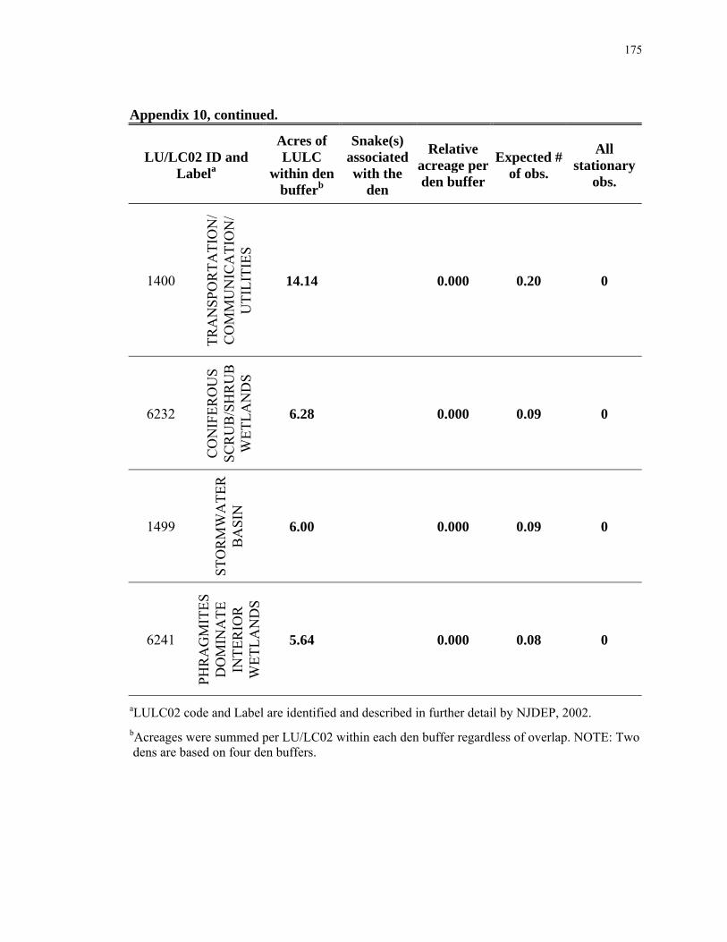
175
Appendix 10, continued.
LU/LC02 ID and Labela
Acres of LULC
within den bufferb
Snake(s) associated with the
den
Relative acreage per den buffer
Expected # of obs.
All stationary
obs.
1400
TRA
NSP
OR
TATI
ON
/ C
OM
MU
NIC
ATI
ON
/ U
TILI
TIES
14.14 0.000 0.20 0
6232
CO
NIF
ERO
US
SCR
UB
/SH
RU
B
WET
LAN
DS
6.28 0.000 0.09 0
1499
STO
RM
WA
TER
B
ASI
N
6.00 0.000 0.09 0
6241
PHR
AG
MIT
ES
DO
MIN
ATE
IN
TER
IOR
W
ETLA
ND
S
5.64 0.000 0.08 0
aLULC02 code and Label are identified and described in further detail by NJDEP, 2002. bAcreages were summed per LU/LC02 within each den buffer regardless of overlap. NOTE: Two dens are based on four den buffers.
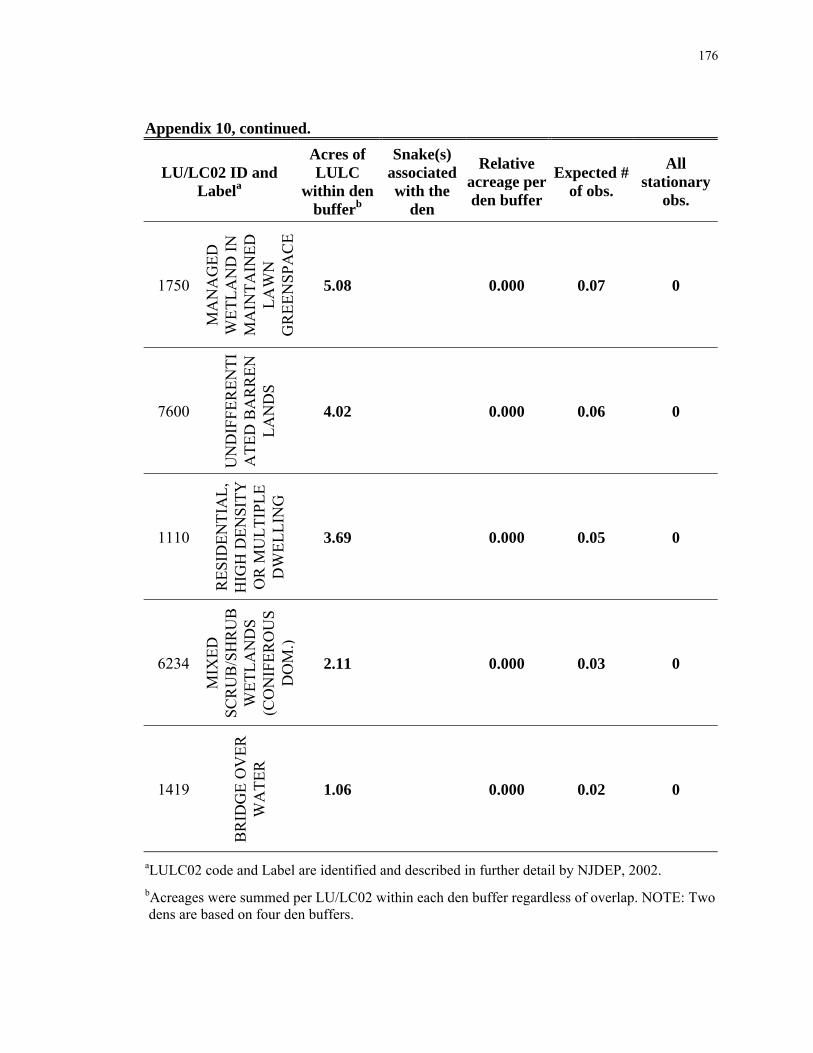
176
Appendix 10, continued.
LU/LC02 ID and Labela
Acres of LULC
within den bufferb
Snake(s) associated with the
den
Relative acreage per den buffer
Expected # of obs.
All stationary
obs.
1750
MA
NA
GED
W
ETLA
ND
IN
MA
INTA
INED
LA
WN
G
REE
NSP
AC
E 5.08 0.000 0.07 0
7600
UN
DIF
FER
ENTI
ATE
D B
AR
REN
LA
ND
S
4.02 0.000 0.06 0
1110
RES
IDEN
TIA
L,
HIG
H D
ENSI
TY
OR
MU
LTIP
LE
DW
ELLI
NG
3.69 0.000 0.05 0
6234
MIX
ED
SCR
UB
/SH
RU
B
WET
LAN
DS
(CO
NIF
ERO
US
DO
M.)
2.11 0.000 0.03 0
1419
BR
IDG
E O
VER
W
ATE
R
1.06 0.000 0.02 0
aLULC02 code and Label are identified and described in further detail by NJDEP, 2002. bAcreages were summed per LU/LC02 within each den buffer regardless of overlap. NOTE: Two dens are based on four den buffers.

177
Appendix 11. Land use cover types containing snake observations not captured by The Landscape Project, Version 3.0 Highlands.
Habitat type (per LU/LC02a) # of Observations Herbaceous wetlands 4
Natural lakeb 1 Cropland/pastureland 1
Residential, single unit 22 Other urban or built up 2 Athletic fields/schools 1
Transportation/communication 5 aLU/LC02 (Land Use Land Cover 2002) per NJ Department of Environmental Protection (2002; modified descriptions of Anderson 1976). bObservation was made during a dry year; snake was foraging at the lake edge in marsh-like habitat.

178
LITERATURE CITED Anderson, G.S. and B.J. Danielson. 1997. The effects of landscape composition and
physiognomy on metapopulation size: the role of corridors. Landscape Ecology 12: 261-271.
Anderson, J.R., E.E. Hardy, J.T. Roach and R.E. Witmer. 1976. A land use and land
cover classification system for use with remote sensor data. U.S. Geological Survey Professional Paper 964. 28pp.
Andrews, K.M. and J.W. Gibbons. 2005. How do highways influence snake movement?
Behavioral responses to roads and vehicles. Copeia 2005 (4): 772-782. Andrews, K.M., J.W. Gibbons, and D.M. Jochimsen. 2006. Literature Synthesis of the
effects of roads and vehicles on amphibians and reptiles. Federal Highway Administration (FHWA), U.S. Department of Transportation, Report NO. FHWA-HEP-08-005. Washington, D.C. 151pp.
Aspinall, R. and N. Veitch. 1993. Habitat mapping from satellite imagery and wildlife
survey data using a Bayesian modeling procedure in a GIS. Photogrammetric Engineering and Remote Sensing 59(4): 537-543.
Bennett, A.F. 1998, 2003. Habitat fragmentation and the consequences for wildlife. Pp.
13-36, In Linkages in the Landscape: The Role of Corridors and Connectivity in Wildlife Conservation. IUCN, Gland, Switzerland and Cambridge, UK. xiv + 254 pp.
Bonnet, X., G. Naulleau and R. Shine. 1999. The dangers of leaving home: dispersal and
mortality in snakes. Biological Conservation 89 (1999): 39-50. Breisch, A. R. 1992. Summary of state/provincial regulations concerning the timber
rattlesnake in the northeast. Pages 7–8 in T. F. Tyning, editor. Conservation of the timber rattlesnake in the northeast. Massachusetts. Audubon Society, Lincoln, Massachusetts, USA.
Brown, W.S. 1992. Emergence, ingress and seasonal captures at dens of northern timber
rattlesnake (Crotalus horridus). Pp. 251-258, In J.A. Campbell and E.D. Brodie, Jr. (eds.). Biology of the Pitvipers. Selva Press, Tyler, Texas. 467 pp.
----------------. 1993 Biology, status and management of the timber rattlesnake (Crotalus
horridus): a guide for conservation. SSAR Herpetological Circular 22:1-78. ----------------, D.W. Pyle, K.R. Greene and J.B. Friedlaender. 1982. Movements and
temperature relationships of timber rattlesnakes (Crotalus horridus) in Northeastern New York. Journal of Herpetology 16(2): 151-161.

179
---------------- and F.M. MacLean. 1983. Conspecific scent-trailing by newborn timber rattlesnakes, Crotalus horridus. Herpetologica 39(4): 430-436.
Browning, D.M., S.J. Beaupre and L. Duncan. 2005. Using partitioned Mahalanobis
D2(K) to formulate a GIS-based model of timber rattlesnake hibernacula. Journal of Wildlife Management 69(1): 33-44.
Bushar, L.M., H.K. Reinert and L. Gelbert. 1998. Genetic variation and gene flow
within and between local populations of the timber rattlesnake, Crotalus horridus. Copeia 1998(2): 411-422.
Cook, J.G., T.W. Stutzman, C.W. Bowers, K.A. Brenner and L.L. Irwin. 1995. Spherical
densiometers produce biased estimates of forest canopy cover. Wildlife Society Bulletin 23(4): 711-717.
DeLaune, M.G. 2003. X-tools ArcView Extension (version 09/15/2003). Oregon
Department of Forestry. Dijak, W.D., C.D. Rittenhouse, M.A. Larson, F.R.Thompson, III and J.J. Millspaugh.
2007. Landscape habitat suitability index software. Journal of Wildlife Management 71(2): 668-670.
Endangered and Nongame Species Conservation Act (ENSCA), N.J.S.A. 23:2A-1 to -20. Ernst, C.H. and R.W. Barbour. 1989. Crotalus horridus, timber rattlesnakes. Pp. 211-
214. In Snakes of Eastern North America. George Mason University Press, Virginia. 282 pp.
Fielding, A.H. and J.F. Bell. 1997. A review of methods for the assessment of predication
errors in conservation presence/absence models. Environmental Conservation 24(1): 38-49.
Flather, C.H. and J.R. Sauer. 1996. Using landscape ecology to test hypotheses about
large-scale abundance patterns in migratory birds. Ecology 77(1): 28-35. Furman, J. 2007. Bounty hunting. Pp. 84-103. In Timber Rattlesnakes in Vermont and
New York: Biology, History, and the Fate of an Endangered Species. University Press of New England, Lebanon, New Hampshire. 207 pp.
Galligan, J.H. and W.A. Dunson. 1979. Biology and status of timber rattlesnake
(Crotalus horridus) populations in Pennsylvania. Biological Conservation 15: 13-58.
Gibbons, J.W, D.E. Scott, T.J. Ryan, K.A. Buhlmann, T.D. Tuberville, B.S. Metts, J.L.
Greene, T. Mills, Y. Leiden, S. Poppy and C.T. Winne. 2000. The global decline of reptiles, déjà vu amphibians. BioScience 50: 653-666.
180
Gibson, L.A., B.A. Wilson, D.M. Cahill and J. Hill. 2004. Spatial predication of rufous bristlebird habitat in a coastal heathland: a GIS-based approach. Journal of Applied Ecology 41: 213-223.
Jennings, S.B., N.D. Brown and D. Sheil. 1999. Assessing forest canopies and
understorey illumination: canopy closure, canopy cover and other measures. Forestry 72(1): 59-73.
Hilty, J.A., W.Z. Lidicker, Jr. and A.M. Merenlender. 2006. Background: Land-use
changes and habitat loss and Understanding fragmentation. Pp. 1-48, In Corridor Ecology, The Science and Practice of Linking Landscapes for Biodiversity Conservation. Island Press, Washington, D.C. 323 pp.
Kéry, M. 2002. Inferring the absence of a species – a case study of snakes. Journal of
Wildlife Management 66(2): 330-338. Kienast, F. 1993. Analysis of historic landscape patterns with a Geographical
Information System – a methodological outling. Landscape Ecology 8(2): 103- 118.
Klauber, L.M. 1956. Rattlesnakes, Vols. 1 and 2. Berkeley, University of California
Press. Pp. 1476. Landreth, H. F. 1973. Orientation and behavior of the rattlesnake, Crotalus atrox.
Copeia 1973: 26-31. Lemmon, P.E. 1956. A spherical densiometer for estimating forest overstory density.
Forestry Science 2: 314-320. Martin, W.H. 1992a. Phenology of the timber rattlesnake (Crotalus horridus) in an
unglaciated section of the Appalachian Mountains. Pp. 259-277, In J.A. Campbell and E.D. Brodie, Jr. (eds.). Biology of the Pitvipers. Selva Press, Tyler, Texas.
----------------. 1992b. The timber rattlesnake: its distribution and natural history. Pp. 13-
22, In T. F. Tyning (ed.), Conservation of the Timber Rattlesnake in the Northeast. Massachusetts Audubon Society, Lincoln, MA.
----------------. 1993. Reproduction of the timber rattlesnake (Crotalus horridus) in the
Appalachian Mountains. Journal of Herpetology 27(2): 133-143.
----------------. 2002. Life history constraints on the timber rattlesnake (Crotalus horridus) at its climatic limits. Pp. 285-306, In G.W. Schuett, M. Höggren, M.E. Douglas, and H.W. Greene (eds.). Biology of the Vipers. Eagle Mountain Publishing, Eagle Mountain, Utah.

181
McGowan, E., K. Michell, J.W. Jaycox. 2006. Non-surgical attachment of external transmitters on timber rattlesnakes for monitoring short-term movements. Northeast Natural History Conference, Albany, N.Y. (Presented by K. Michell)
Minnesota Department of Natural Resources. DNR Garmin Extension (version 4.42,
08/06/2004). Downloadable versions available online at: www.dnr.state.mn.us/mis/gis/tools/arcview/extensions.html
New Jersey Department of Environmental Protection (NJDEP), Office of Information
Resources Management (OIRM), Bureau of Geographic Information Systems (BGIS). 1995. Land use/Land cover Update.
New Jersey Department of Environmental Protection (NJDEP), Office of Information
Resources Management (OIRM), Bureau of Geographic Information Systems (BGIS). 2002. Digital Elevation Model.
New Jersey Department of Environmental Protection (NJDEP), Office of Information
Resources Management (OIRM), Bureau of Geographic Information Systems (BGIS). 2002. NJDEP Land use/Land cover Update.
New Jersey Department of Transportation (NJDOT), Bureau of Transportation Data
Development (BTDD). 2008. NJ Roadway Network 2008. Available online at: www.state.nj.us/transportation/gis/map.shtm.
New Jersey Division of Fish and Wildlife, Endangered and Nongame Species Program.
1999-2000. Timber Rattlesnake Project, Kittatinny Ridge. Unpublished data. NJ Highlands Council. Highlands Regional Master Plan, September 8, 2008. Chester,
New Jersey. Pp. 489. Niles, LJ, M. Valent, J. Tash, and J. Myers. 2001. New Jersey's The Landscape Project:
Wildlife habitat Mapping for Community Land-use Planning and Endangered Species Conservation. Project report. Endangered and Nongame Species Program, NJ DFW, NJ DEP. 20 pp.
Parent, C. and P.J. Weatherhead. 2000. Behavioral and life history responses of eastern
massasauga rattlesnakes (Sistrurus catenatus catenatus) to human disturbance. Oecologia 125: 170-178.
Pearce, J. and S. Ferrier. 2000. Evaluating the predictive performance of habitat models
developed using logistic regression. Ecological Modelling 133(2000): 225-245. Pereira, J.M.C. and R.M. Itami. 1991. GIS-based habitat modeling using logistic
multiple regression: A study of the Mt. Graham red squirrel. Photogrammetric Engineering and Remote Sensing 57(11): 1475-1486.
182
Peterson, A. 1990. Ecology and management of a timber rattlesnake (Crotalus horridus L.) population in South-Central New York State. New York State Museum Bulletin 471: 255-261.
Reinert, H.K. 1984a. Habitat variation within sympatric snake populations. Ecology 65:
1673-1682. ----------------. 1984b. Habitat separation between sympatric snake populations. Ecology
65(2): 478-486. ----------------. 1992. Radiotelemetric field studies of pitvipers: data acquisition and
analysis. Pp. 185-197, In J.A. Campbell and E.D. Brodie, Jr. (eds.), Biology of the pitvipers. Selva, Tyler, Texas.
---------------- and D. Cundall. 1982. An improved surgical implantation method for
radio-tracking snakes. Copeia 3:702-705. ---------------- and R.R. Rupert, Jr. 1999. Impacts of translocation on behavior and
survival of timber rattlesnakes, Crotalus horridus. Journal of Herpetology 33(1): 45-61.
---------------- and R.T. Zappalorti. 1988. Timber rattlesnakes (Crotalus horridus) of the
Pine Barrens: Their movement patterns and habitat preference. Copeia 4: 964- 978.
Rittenhouse, C.D., W.D. Dijak, F.R. Thompson, III and J.J. Millspaugh. 2007.
Development of Landscape-level habitat suitability models for ten wildlife species in the central hardwoods region. Pp. 24-27, In Gen. Tech. Rep. NRS-4. Newton Square, PA: U.S. Department of Agriculture, Forest Service, Northern Research Station.
Roseberry, J. L., B.J. Richards and T.P. Hollenhorst. 1994. Assessing the potential
impact of conservation reserve program lands on bobwhite habitat using remote sensing, GIS, and habitat modeling. Photogrammetric Engineering and Remote Sensing 60(9): 1139-1143.
Steen, D.A., L.L. Smith, L.M. Conner, J.C. Brock and S.K. Hoss. 2007. Habitat use of
sympatric rattlesnake species within the Gulf Coastal Plain. Journal of Wildlife Management 71(3): 759-764.
Tuxbury, S.M. and M. Salmon. 2005. Competitive interactions between artificial lighting
and natural cues during sea finding by hatchling marine turtles. Biological Conservation 121: 311 – 316.
183
United State Department of Agriculture (USDA), Soil Survey Staff, Natural Resources Conservation Service. Soil Survey Geographic (SSURGO) Database for [Sussex, Passaic, Warren, Morris and Bergen Counties, New Jersey]. Available online at http://soildatamart.nrcs.usda.gov accessed [04/14/2004].
Waldron, J.L., J.D. Lanham and S.H. Bennett. 2006. Using behaviorally-based seasons to
investigate canebrake rattlesnake (Crotalus horridus) movement patterns and habitat selection. Herpetologica 62(4): 389-398.
Wiegand, T., K.A. Moloney, J. Naves and F. Knauer. 1999. Finding the missing link
between landscape structure and population dynamics: A spatially explicit perspective. American Naturalist 154: 605-627.
Wilson, B. A., J.G. Aberton and T. Reichl. 2001. Effects of fragmented habitat and fire
on the distribution and ecology of the swamp antechinus (Antechinus minimus maritimus) in the eastern Otways, Victoria. Wildlife Research 28(2001): 527-536.
----------------, A. Lewis and J. Aberton. 2002. Spatial model for predicting the presence
of cinnamon fungus (Phytophythora cinnamomi) in sclerophyll vegetation communities in south-eastern Australia. Austral Ecology 28: 108-115.
Winkler, P., G. Fowles, M. Valent and P. Woerner. 2008. New Jersey’s Landscape
Project, (Version 3.0 Highlands): A species-based patch approach to rare and imperiled wildlife habitat mapping for community land-use planning and species conservation. Unpublished booklet prepared for the New Jersey Department of Environmental Protection, Division of Fish and Wildlife, Endangered and Nongame Species Program. 149 pp.