1/33

Project no. 004089

AMMA

African Monsoon Multidisciplinary Analysis Instrument : IP

Thematic Priority : 2.1 Processes studies: Convection and dynamic

4.3 Satellite remote sensing

Du2.1.3.a: ATLAS on a climatology of West African

Mesoscale Convective Systems

Start date of project: 1st January 2003 Duration: 60 months Lead contractor : CNRM Coordinator of deliverable : Mireille Tomasini Evolution of deliverable Due date : M18 Date of first draft : M15 Start of review : Deliverable accepted :

Project co-funded by the European Commission within the Sixth Framework Programme (2002-2006)

Dissemination Level PU Public X PP Restricted to other programme participants (including the Commission Services) RE Restricted to a group specified by the consortium (including the Commission Services) CO Confidential, only for members of the consortium (including the Commission Services)

2/33

ATLAS on a climatology of West African Mesoscale Convective Systems

M. TOMASINI1, J-P. LAFORE1, C. PIRIOU1, R. ROCA2, K. RAMAGE2, H. LAURENT3, C.

MOREL1, S. SENESI1

Abstract

An automated method from the satellite infrared imagery allows us to catch MCS. The main characteristics of the Rapidly Developing Thunderstorms algorithm, like an adaptative temperature threshold, already operational at Météo-France within the SAF-Now Casting, are described.

Thanks to the description of the MCS life cycle provided by the RDT tracking software, a classification into four categories adapted to the West Africa is proposed, based on the MCS duration and propagation speed. Then a climatology on MCS has been realized on eight years (1996-2003), around several specific sites of West Africa (Agoufou, Bamako, Cotonou, Dakar, Niamey, Ouadagoudou, Parakou) like:

• The seasonal cycle of the number of trajectories crossing a site and its inter-annual variability

• The diurnal cycle of the number of trajectories crossing a site • The spatial distribution of the nebulosity

Please find the several quoted external files at the address: : http://aoc.amma-

international.org/ under Observations/Climatology.

1 Météo-France, 42 av. G. Coriolis, 31057 Toulouse Cedex 01, France (mireille.tomasini@meteo.fr) 2 Laboratoire de Météorologie Dynamique, École Normale Supérieure, Paris, France 3 LTHE, Domaine Universitaire, BP 53, 38041 Grenoble cedex 9, France

This deliverable aims at guiding the preparation of the wet AMMA SOP in 2006. A better knowledge of the mean characteristics of MCS (Mesoscale Convective Systems), of

their distribution all during the monsoon season and of their inter annual variability, is a crucial information for deciding the date, duration and location of the different periods of observation to get a representative sampling of the MCS. This work already presenting during the SOP preparatory meetings, helped to perform above operational choices. It thus directly contributed to the TT8 implementation plan.

Also the proposed classification of West African MCS will allow to quickly and easily identify

them during the AMMA campaign and its scientific exploitation. The work needed a close collaborationbetween different between three French laboratories

and involved the contribution of two Work Packages (WP2.1 and WP4.3) to properly use satellite data and to develop a classification and a climatology consistent with our knowledge of convective processes.

3/33

I Introduction West Africa is a vast zone where several types of Mesoscale Convective Systems (MCS)

develop according to the latitude, surface conditions and the topography… MCS is usually defined as a single cumuliform4 and well vertically developed cloud or a cluster of such clouds, of typical horizontal extent 100x100 km², the mesoscale, between the local and synoptic scales. Squall lines (Lafore and Moncrieff 1989) of linear type, Mesoscale Convective Complexes (MCC first defined by Maddox 1980) of circular type, Organized Complex Systems (OCS) of Mathon (2001) which give the more precipitations over the Sahelean band (cf. §3.4) and superclusters of Mapes and Houze (1993) which last more than two days belong all to the MCS types. They produce most of the precipitations over the region. Several authors have tried to classify them.

In 1984, Barnes and Sieckman have classified the oceanic MCS according to their speed, in

three classes with thresholds at 3 and 7 m.s-1, thanks to the rawinsonde data from the GATE experiment. The thermodynamical properties of the faster MCS, named squall lines by the authors, are compared to the slow-moving MCS.

Over the oceanic COARE domain, Chen et al. (1996) had separated the cloud clusters according to their maximum size only, thanks to the tracking program of Williams and Houze (1987) with the Japanese Geosynchronous Meteorological Satellite infrared imagery at the fixed temperature of 208 K. This cold threshold is supposed to match the rain core although a threshold of 235 K is sufficient to catch the deep convection systems. Few but long-lived they contribute to the total cloud coverage at the level of 30% (15%) for a duration longer than 24 hours (48 hours respectively).

Over the Sahel, where atmospheric and surface conditions facilitate the maintenance of organized big systems, Mathon et al. (2002) has found that only 12% of the MCS explain 78% of the nebulosity (at the temperature 233 K) and 83% of the rainfalls. Those systems are the largest and last the longest. They are preponderant from June to September. Their cloud cover is modulated by their size, which is emphasized in August. They propagate quickly (faster than 10 m.s-1) towards the west. Mathon and Laurent (2001) have noticed the coincidence between the speed of the African Equatorial Jet (AEJ) and of the MCS.

On the contrary, on the Amazonian region, the study of Laurent et al. (2002), during the wet season too, shows that the coldest clusters (~210 K) last less than 12 hours.

As a consequence, universal criteria to classify MCS are not obvious and previous proposed classifications are not adapted to West Africa. Our goal is to propose a classification of West Africa MCS (§III) in order to quickly and easily identify them during the AMMA campaign and its scientific exploitation.

As the conventional observation network stays poor in Africa, satellite approach with infrared

pictures, seems best suited. An automated method for catching MCS provides a complete description of their life cycle. The main characteristics of the Rapidly Developing Thunderstorms5 algorithm, already operational at Météo-France within the SAF6-Now Casting, are described in section II.

Arnaud et al. (1992) described some convective events (tracking also with an automatic algorithm from satellite pictures) of the year 1989 that produce rain over the EPSAT7-Niger zone. Machado et al. (1992) studied six summers (1983-88) of Meteosat infrared data over West Africa. Mean structural characteristics of MCS are given like their numbers as a function of their radius and 4 at least at its first stage of development because once the tropopause reaching, it spreads horizontally. 5 RDT in english, ISIS for "Instrument de Suivi dans l’Imagerie Satellitale" in french 6 Satellite Application Facilities 7 Estimation des Précipitations par SATellite

4/33

brightness temperature, the correlation between their horizontal and vertical extends, their spatial distribution, their inter-annual and diurnal variability. More recently, the PhD of Mathon (2001) and the HDR8 of Laurent (2005) were dedicated to such a climatology on MCS. But it remains rare and we proposed in section IV, some climatologies on eight years (1996-2003), treated with the RDT tracking software, around several specific sites (Agoufou, Bamako, Cotonou, Dakar, Niamey, Ouadagoudou, Parakou).

II MCS tracking Temporal series of satellite images (§2.1) have been objectively processed with the RDT5

software developed by Météo-France within the EUMETSAT’s SAF-Now casting to follow MCS (Morel and Sénési 2002). Their detection (§2.2), tracking (§2.3), discrimination among other cloud types (§2.4) and properties are explained below. Section 2.6 provides an example of the RDT product.

2.1 Data Meteosat 7 infrared images (10,8 μ channel) are here used with a spatial resolution of 5x5 km²

and a temporal resolution of 30 mn. The geographical domain covers West Africa from 0°N to 19°N and from 42°E to 18°W.

2.2 Detection All known authors use a fixed temperature threshold to detect tropical and equatorial MCS

between –20°C (253 K) and –75°C (198 K) (cf. Mapes and Houze 1993, for a review of the thresholds used). Jobard and Desbois (1992) have chosen the –60°C (213 K) threshold due to its good correlation with the rainfalls in central Sahel. But a confusion with the cirrus cloud type can be made if the single threshold is too cold. The tracking algorithm of the LTHE-LMD defines and follows the MCS at the –40°C (233 K) temperature assuming that 93% of the total cloud coverage can be tracked at this threshold (Mathon and Laurent 2001). Arnaud et al. (1992) used this same fixed threshold to keep only convective clouds that have the more chance to precipitate.

It is worth knowing that in a standard tropical atmosphere 253 K corresponds to a height of 7.9 km, 230 K to 11.3 km and 207 K to 14.7 km (Machado et al. 1992).

In our program, cells are detected and tracked using an adaptative temperature threshold (from –10°C (263 K) to –65°C (208 K)). A cell is a zone of contiguous pixels having a brightness temperature (that is to say the black-body temperature) Tb colder than a temperature threshold Tth=Tb

minimum+3 (+3 to include the cumulus towers). Therefore, Tth varies with the cell stage during the cell life cycle:

warm at the early stages, starting from –10°C (263 K), to improve the detection, increasingly colder Tth following the system development, until –65°C (208 K), to avoid

merging different embedded systems.

2.3 Tracking The trajectory of a cloud system is built from the overlapping of clouds between two successive

infrared images, using an estimation of their speed. It also handles clouds split and merging processes.

8 Habilitation à Diriger des Recherches

5/33

2.4 Discrimination of convective systems among all tracked systems Tests have been made to use the peripheral gradient and the cooling rate along the trajectory to

separate convective from stratiform clouds (Morel and Sénési 2002). Lightening data can also help but such a network is not available on Africa.

In our study over West Africa where most of clouds are of convective origin, it is sufficient to keep only the trajectories that reach an area of 5000 km² at a temperature of -40°C (233 K). This is the minimum size of our MCS: equivalent radius of 40 km.

Mathon and Laurent (2001), like several authors, use the minimum surface (200 pixels or 4200 km² near the equator) as early as the detection. The MCS lifetime is thus undervalued.

2.5 Properties Relevant morphological (surface, ellipticity and orientation of the best-fitting ellipse of the

cell), radiative (minimum and mean temperature, mean temperature gradient) and dynamical properties of the cells (position of the centre of gravity) and of the trajectories (duration, historical record of cells) are saved at different infrared levels.

2.6 Applications Two versions of the RDT software are available corresponding to two different applications:

• Now-casting purposes: The early detection of convective events and the analysis of the trajectories are useful for forecasters and operationally used at Météo-France. The Figure 1 illustrates this product as proposed to the user on its terminal for a case over West Africa the first of August 2004 at 21 UTC. The trajectories paths are traced in yellow lines. The MCS are outlined at different stages. Once you have clicked inside its contour, its main characteristics (see the right grey box) and the time evolution of typical temperatures and areas show off. Animations are possible too. This product runs already every day with the MSG29 pictures over West Africa. The results are available for consultation on the web site : http://aoc.amma-international.org/observation/mcstracking/. It will be available to the African Operational Centre at Niamey during the Special Observation Period in the summer 2006. Moreover, the images treated with the RDT software are available to the AMMA community for the years 1999, 2000 and 2004 on the web site: http://ammasat.ipsl.polytechnique.fr/.

• Climatology: Trajectories properties are kept in ASCII files so that everybody can easily performed climatological studies. An example of such a file (File 1), its description (File 2) and a FORTRAN 90 file to read it (File 3) are provided. Eight years of data from 1996 to 2003 are available to the AMMA community on request.

9 Météosat Seconde Génération (METEOSAT8)

6/33

Stage: coolingTminimum = -77°CTaverage = -69°CT trend = -4°C/hSurf. trend = -16900 km²/hExpansion = -43,4%Duration = 300mnArea = 6 800 km²Max. area = 14 100 km²Tminimum= -65°C at 19h30Speed = 24,6 m/sCG lat = 13,53°CG lon = 8,25 °

Figure 1: RDT product in its now-casting version. See the users’ guide on the AMMASAT site for the legend.

7/33

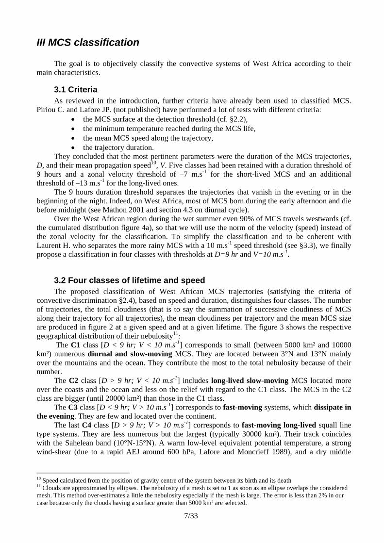
III MCS classification The goal is to objectively classify the convective systems of West Africa according to their

main characteristics.

3.1 Criteria As reviewed in the introduction, further criteria have already been used to classified MCS.

Piriou C. and Lafore JP. (not published) have performed a lot of tests with different criteria: • the MCS surface at the detection threshold (cf. §2.2), • the minimum temperature reached during the MCS life, • the mean MCS speed along the trajectory, • the trajectory duration.

They concluded that the most pertinent parameters were the duration of the MCS trajectories, D, and their mean propagation speed10, V. Five classes had been retained with a duration threshold of 9 hours and a zonal velocity threshold of –7 m.s-1 for the short-lived MCS and an additional threshold of –13 m.s-1 for the long-lived ones.

The 9 hours duration threshold separates the trajectories that vanish in the evening or in the beginning of the night. Indeed, on West Africa, most of MCS born during the early afternoon and die before midnight (see Mathon 2001 and section 4.3 on diurnal cycle).

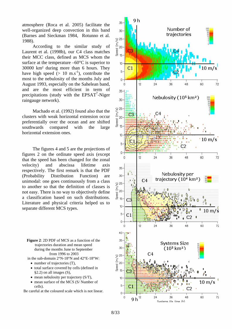
Over the West African region during the wet summer even 90% of MCS travels westwards (cf. the cumulated distribution figure 4a), so that we will use the norm of the velocity (speed) instead of the zonal velocity for the classification. To simplify the classification and to be coherent with Laurent H. who separates the more rainy MCS with a 10 m.s-1 speed threshold (see §3.3), we finally propose a classification in four classes with thresholds at D=9 hr and V=10 m.s-1.

3.2 Four classes of lifetime and speed The proposed classification of West African MCS trajectories (satisfying the criteria of

convective discrimination §2.4), based on speed and duration, distinguishes four classes. The number of trajectories, the total cloudiness (that is to say the summation of successive cloudiness of MCS along their trajectory for all trajectories), the mean cloudiness per trajectory and the mean MCS size are produced in figure 2 at a given speed and at a given lifetime. The figure 3 shows the respective geographical distribution of their nebulosity11:

The C1 class [D < 9 hr; V < 10 m.s-1] corresponds to small (between 5000 km² and 10000 km²) numerous diurnal and slow-moving MCS. They are located between 3°N and 13°N mainly over the mountains and the ocean. They contribute the most to the total nebulosity because of their number.

The C2 class [D > 9 hr; V < 10 m.s-1] includes long-lived slow-moving MCS located more over the coasts and the ocean and less on the relief with regard to the C1 class. The MCS in the C2 class are bigger (until 20000 km²) than those in the C1 class.

The C3 class [D < 9 hr; V > 10 m.s-1] corresponds to fast-moving systems, which dissipate in the evening. They are few and located over the continent.

The last C4 class [D > 9 hr; V > 10 m.s-1] corresponds to fast-moving long-lived squall line type systems. They are less numerous but the largest (typically 30000 km²). Their track coincides with the Sahelean band (10°N-15°N). A warm low-level equivalent potential temperature, a strong wind-shear (due to a rapid AEJ around 600 hPa, Lafore and Moncrieff 1989), and a dry middle

10 Speed calculated from the position of gravity centre of the system between its birth and its death 11 Clouds are approximated by ellipses. The nebulosity of a mesh is set to 1 as soon as an ellipse overlaps the considered mesh. This method over-estimates a little the nebulosity especially if the mesh is large. The error is less than 2% in our case because only the clouds having a surface greater than 5000 km² are selected.

8/33

atmosphere (Roca et al. 2005) facilitate the well-organized deep convection in this band (Barnes and Sieckman 1984, Rotunno et al. 1988).

According to the similar study of Laurent et al. (1998b), our C4 class matches their MCC class, defined as MCS whom the surface at the temperature –60°C is superior to 30000 km² during more than 6 hours. They have high speed (> 10 m.s-1), contribute the most to the nebulosity of the months July and August 1993, especially on the Sahelean band, and are the most efficient in term of precipitations (study with the EPSAT7-Niger raingauge network).

Machado et al. (1992) found also that the clusters with weak horizontal extension occur preferentially over the ocean and are shifted southwards compared with the large horizontal extension ones.

The figures 4 and 5 are the projections of figures 2 on the ordinate speed axis (except that the speed has been changed for the zonal velocity) and abscissa lifetime axis respectively. The first remark is that the PDF (Probability Distribution Function) are unimodal: one goes continuously from a class to another so that the definition of classes is not easy. There is no way to objectively define a classification based on such distributions. Literature and physical criteria helped us to separate different MCS types.

Figure 2: 2D PDF of MCS as a function of the trajectories duration and mean speed during the months June to September

from 1996 to 2003 in the sub-domain 2°N-18°N and 42°E-18°W:

• number of trajectories (T), • total surface covered by cells (defined in

§2.2) on all images (S), • mean nebulosity per trajectory (S/T), • mean surface of the MCS (S/ Number of

cells). Be careful at the coloured scale which is not linear.

9/33

Figure 3a

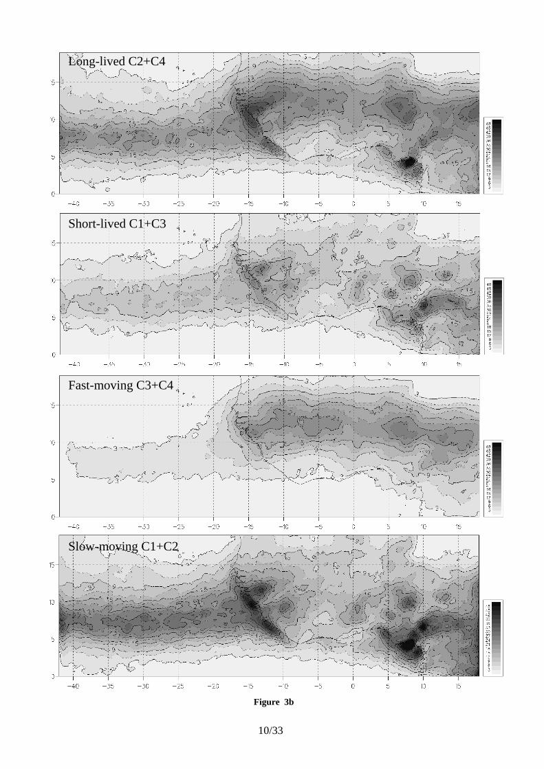
10/33

Figure 3b

Fast-moving C3+C4

Short-lived C1+C3

Long-lived C2+C4

Slow-moving C1+C2

11/33

The distributions as a function of the trajectories mean zonal velocity (figures 4) are:

• Gaussian curves for the number of MCS trajectories with a maximum at –5.5 m.s-1 and a median at –6 m.s-1 (figure 4a),

• Gaussian curves for the total nebulosity with a peak at –8 m.s-1 and a median at –8.5 m.s-1 (figure 4b),

• not Gaussian curves for the nebulosity per trajectory (figure 4c) or for the MCS size (figure 4d) where the peaks are shifted towards the high westwards velocity (-18 m.s-1).

The nebulosity per trajectory and the size of the systems increase strongly with the high westwards velocity from –10 m.s-1, showing that there is a change in the MCS structure when they move quickly. Our cloudiness and system sizes are relatively weak compared to the literature because of the adaptative temperature threshold (cf. §2.2). Notice also the high inter-annual variability, which will be studied in section 4.2.

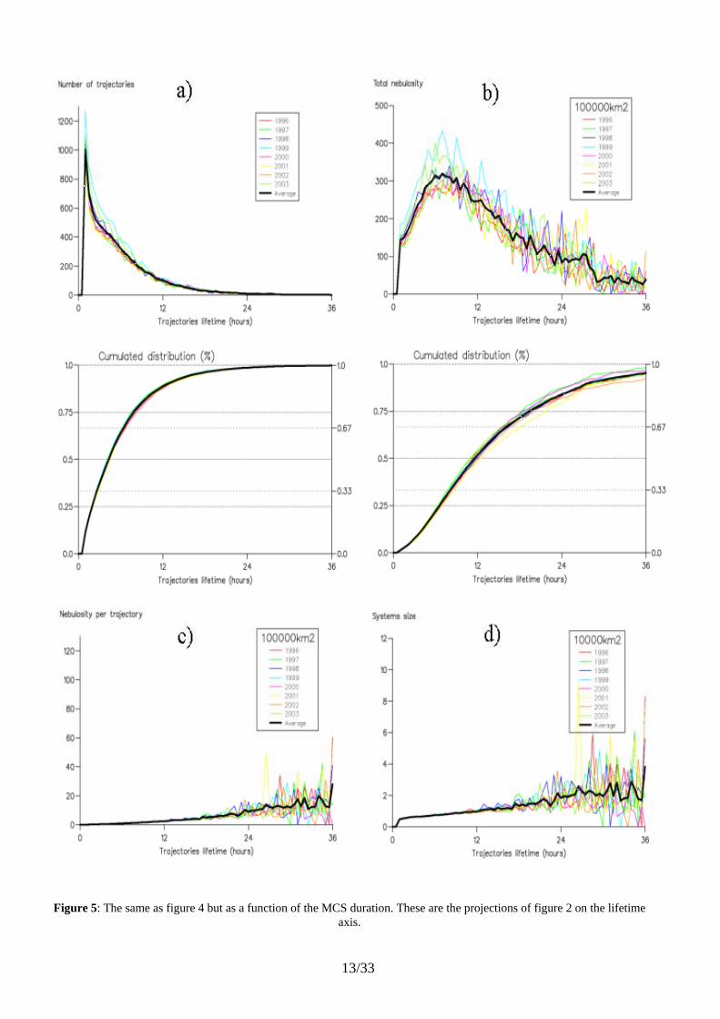
Figures 5 are the PDF versus the duration. The shortest trajectories are the more numerous with half of them lasting less than 4.5 hours (figure 5a). But the peak of total nebulosity occurs between 6 and 9 hours and half of the nebulosity is explained by trajectories lasting more than 11.5 hours (figure 5b). On the other hand, the nebulosity per trajectory (figure 5c) and the mean MCS size (figure 5d) increase linearly with the MCS lifetime before saturation around 36 hours. The slope for the mean MCS size is 417 km² per hour of lifetime. Again we should notice the strong inter-annual variability.

Finally, fast-moving and long-lived clusters (C4 class) are few over West Africa (20% of the MCS moves faster than 10 m.s-1, cf. figure 4a, 10% lasts more than 12 hours and 20% more than 9 hours, cf. figure 5a). However, as they are known to bring annual cyclic saving rains, they have a significant impact on the environment of the Sahelean band. Others MCS types, more numerous and more localized, cumulate the two-third of the nebulosity for the slowest (> -10 m.s-1, cf. figure 4b) or the shortest (< 16 hours, cf. figure 5b).

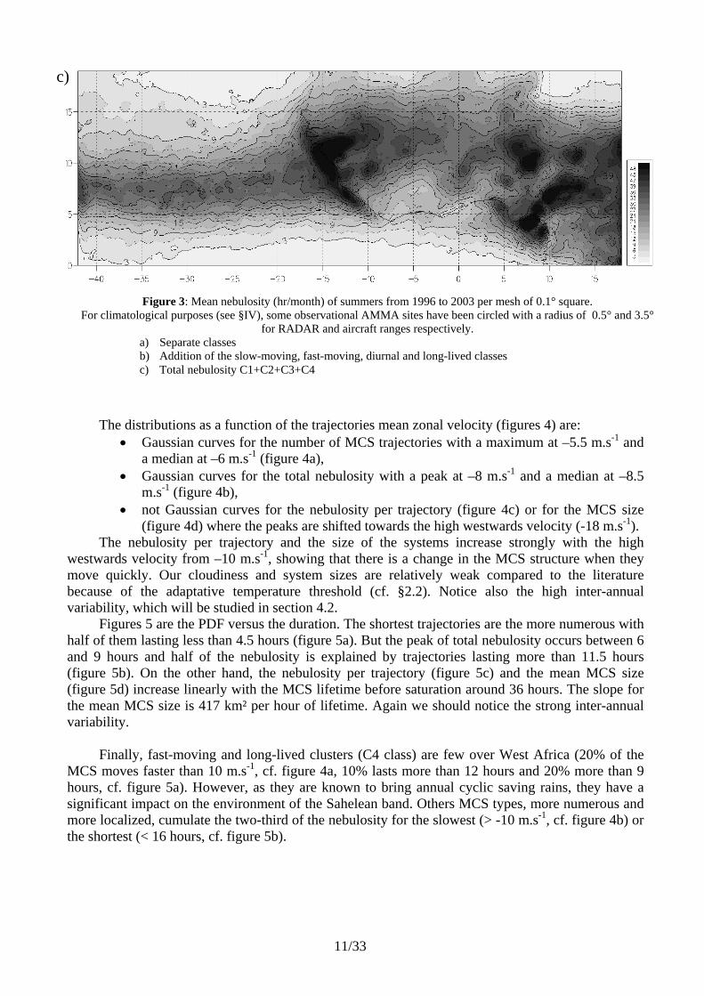
Figure 3: Mean nebulosity (hr/month) of summers from 1996 to 2003 per mesh of 0.1° square. For climatological purposes (see §IV), some observational AMMA sites have been circled with a radius of 0.5° and 3.5°

for RADAR and aircraft ranges respectively. a) Separate classes b) Addition of the slow-moving, fast-moving, diurnal and long-lived classes c) Total nebulosity C1+C2+C3+C4

c)

12/33

Figure 4: Distribution as a function of the zonal velocity. These are the projections of figure 2 on the speed axis: a) Number of trajectories (T, with its cumulated distribution), b) Total cloud coverage (S, with its cumulated distribution), c) Nebulosity

per trajectory (S/T), d) Mean size of the MCS (S/Number of cells). Each curves correspond to the different summers of the years between 1996 and 2003 and the curve in black is their average.

The studied sub-domain stands between 2°N-18°N and 42°E-18°W.

13/33

Figure 5: The same as figure 4 but as a function of the MCS duration. These are the projections of figure 2 on the lifetime axis.

14/33

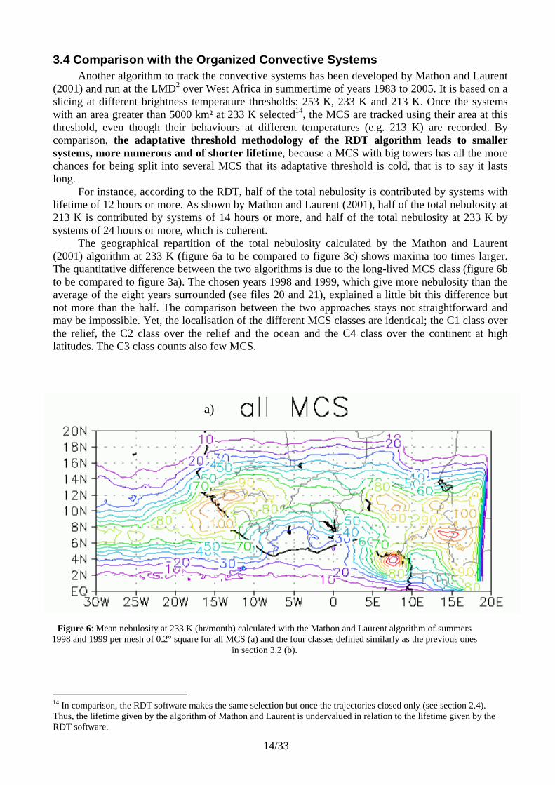
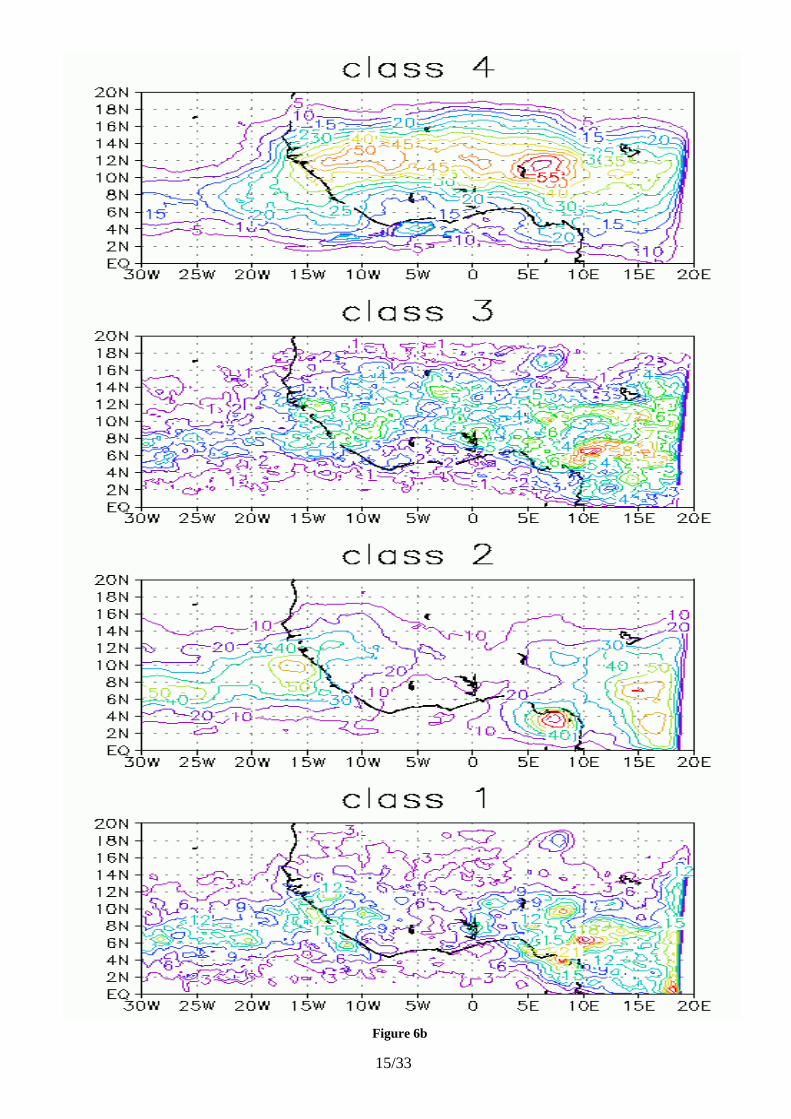
3.4 Comparison with the Organized Convective Systems Another algorithm to track the convective systems has been developed by Mathon and Laurent

(2001) and run at the LMD2 over West Africa in summertime of years 1983 to 2005. It is based on a slicing at different brightness temperature thresholds: 253 K, 233 K and 213 K. Once the systems with an area greater than 5000 km² at 233 K selected14, the MCS are tracked using their area at this threshold, even though their behaviours at different temperatures (e.g. 213 K) are recorded. By comparison, the adaptative threshold methodology of the RDT algorithm leads to smaller systems, more numerous and of shorter lifetime, because a MCS with big towers has all the more chances for being split into several MCS that its adaptative threshold is cold, that is to say it lasts long.

For instance, according to the RDT, half of the total nebulosity is contributed by systems with lifetime of 12 hours or more. As shown by Mathon and Laurent (2001), half of the total nebulosity at 213 K is contributed by systems of 14 hours or more, and half of the total nebulosity at 233 K by systems of 24 hours or more, which is coherent.

The geographical repartition of the total nebulosity calculated by the Mathon and Laurent (2001) algorithm at 233 K (figure 6a to be compared to figure 3c) shows maxima too times larger. The quantitative difference between the two algorithms is due to the long-lived MCS class (figure 6b to be compared to figure 3a). The chosen years 1998 and 1999, which give more nebulosity than the average of the eight years surrounded (see files 20 and 21), explained a little bit this difference but not more than the half. The comparison between the two approaches stays not straightforward and may be impossible. Yet, the localisation of the different MCS classes are identical; the C1 class over the relief, the C2 class over the relief and the ocean and the C4 class over the continent at high latitudes. The C3 class counts also few MCS.

14 In comparison, the RDT software makes the same selection but once the trajectories closed only (see section 2.4). Thus, the lifetime given by the algorithm of Mathon and Laurent is undervalued in relation to the lifetime given by the RDT software.

Figure 6: Mean nebulosity at 233 K (hr/month) calculated with the Mathon and Laurent algorithm of summers 1998 and 1999 per mesh of 0.2° square for all MCS (a) and the four classes defined similarly as the previous ones

in section 3.2 (b).

a)

15/33

Figure 6b

16/33

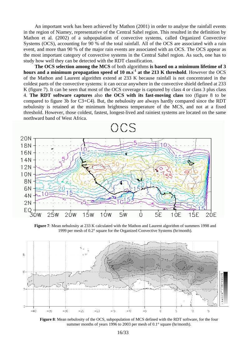
An important work has been achieved by Mathon (2001) in order to analyse the rainfall events in the region of Niamey, representative of the Central Sahel region. This resulted in the definition by Mathon et al. (2002) of a subpopulation of convective systems, called Organized Convective Systems (OCS), accounting for 90 % of the total rainfall. All of the OCS are associated with a rain event, and more than 90 % of the major rain events are associated with an OCS. The OCS appear as the most important category of convective systems in the Central Sahel region. As such, one has to study how well they can be detected with the RDT classification.

The OCS selection among the MCS of both algorithms is based on a minimum lifetime of 3 hours and a minimum propagation speed of 10 m.s-1 at the 213 K threshold. However the OCS of the Mathon and Laurent algorithm extend at 233 K because rainfall is not concentrated in the coldest parts of the convective systems: it can occur anywhere in the convective shield defined at 233 K (figure 7). It can be seen that most of the OCS coverage is captured by class 4 or class 3 plus class 4. The RDT software captures also the OCS with its fast-moving class too (figure 8 to be compared to figure 3b for C3+C4). But, the nebulosity are always hardly compared since the RDT nebulosity is retained at the minimum brightness temperature of the MCS, and not at a fixed threshold. However, those coldest, fastest, longest-lived and rainiest systems are located on the same northward band of West Africa.

Figure 7: Mean nebulosity at 233 K calculated with the Mathon and Laurent algorithm of summers 1998 and 1999 per mesh of 0.2° square for the Organized Convective Systems (hr/month).

Figure 8: Mean nebulosity of the OCS, subpopulation of MCS defined with the RDT software, for the four summer months of years 1996 to 2003 per mesh of 0.1° square (hr/month).

17/33

IV MCS climatology In this paragraph, we present the diurnal cycle (§4.3), seasonal cycle (§4.1) and the inter-annual

variability (§4.2) of the number of trajectories over some sites of West Africa for the June to September months of the eight years period (1996-2003), by distinguishing classes.

4.1 Seasonal cycle Figures 9 and 10 present the number of trajectories per day crossing a disc of radius 3.5° and

0.5° respectively around Niamey. The same graphs are available for Agoufou (File 4), Bamako (File 5), Cotonou (File 6), Dakar (File 7), Ouadagoudou (File 9) and Parakou (File 10). Other sites (or disc sizes) may be available on request.

Note that the method is very sensible to: • the radius because the area varies like its square. Moreover, the larger the radius is,

the more chance one has to catch different types of MCS due to a change in the environment. For example, based at Niamey, an aircraft (action range of 3.5°) can encounter, on average, 5 to 7 MCS per day during the wet period (figure 9c) whereas a RADAR (range of 0.5°) tracks twenty times less MCS (figure 10).

• the intersection method between the area around the site and the MCS because some MCS are as large as this area. To catch the core rain, we count one more trajectory in the disc if, at least one time during its life, the MCS centre of mass intersects the disc.

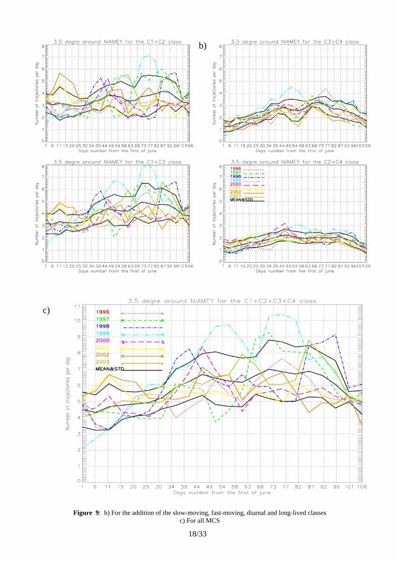
Figure 9: Number of trajectories per day crossing over a disc of a radius 3.5° around NIAMEY as a function of the day from the first of June until the 15 of September. Average over 15 days every 5 days.

The coloured curves correspond to the 8 years. Their average and standard deviation are in black. a) For each class

a)

18/33

Figure 9: b) For the addition of the slow-moving, fast-moving, diurnal and long-lived classes c) For all MCS

b)

c)

19/33

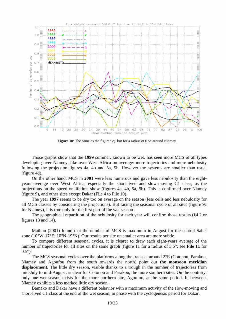
Those graphs show that the 1999 summer, known to be wet, has seen more MCS of all types

developing over Niamey, like over West Africa on average: more trajectories and more nebulosity following the projection figures 4a, 4b and 5a, 5b. However the systems are smaller than usual (figure 4d).

On the other hand, MCS in 2001 were less numerous and gave less nebulosity than the eight-years average over West Africa, especially the short-lived and slow-moving C1 class, as the projections on the speed or lifetime show (figures 4a, 4b, 5a, 5b). This is confirmed over Niamey (figure 9), and other sites except Dakar (File 4 to File 10).

The year 1997 seems to be dry too on average on the season (less cells and less nebulosity for all MCS classes by considering the projections). But facing the seasonal cycle of all sites (figure 9c for Niamey), it is true only for the first part of the wet season.

The geographical repartition of the nebulosity for each year will confirm those results (§4.2 or figures 13 and 14).

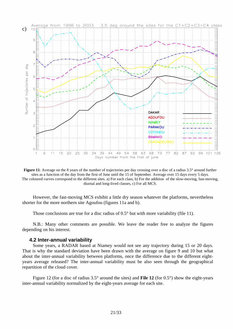
Mathon (2001) found that the number of MCS is maximum in August for the central Sahel

zone (10°W-17°E; 10°N-19°N). Our results per site on smaller area are more subtle. To compare different seasonal cycles, it is clearer to draw each eight-years average of the

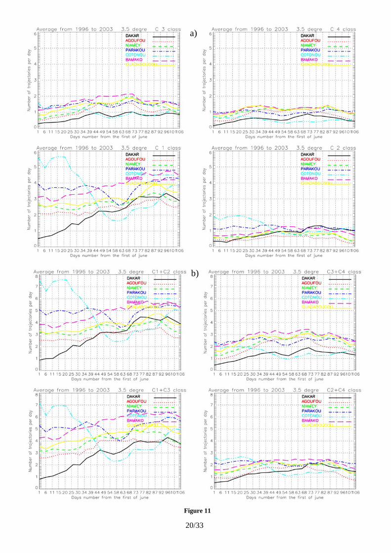
number of trajectories for all sites on the same graph (figure 11 for a radius of 3.5°; see File 11 for 0.5°).

The MCS seasonal cycles over the platforms along the transect around 2°E (Cotonou, Parakou, Niamey and Agoufou from the south towards the north) point out the monsoon meridian displacement. The little dry season, visible thanks to a trough in the number of trajectories from mid-July to mid-August, is clear for Cotonou and Parakou, the more southern sites. On the contrary, only one wet season exists for the more northern site, Agoufou, at the same period. In between, Niamey exhibits a less marked little dry season.

Bamako and Dakar have a different behavior with a maximum activity of the slow-moving and short-lived C1 class at the end of the wet season, in phase with the cyclogenesis period for Dakar.

Figure 10: The same as the figure 9c) but for a radius of 0.5° around Niamey.

20/33

a)

b)

Figure 11

21/33

However, the fast-moving MCS exhibit a little dry season whatever the platforms, nevertheless

shorter for the more northern site Agoufou (figures 11a and b). Those conclusions are true for a disc radius of 0.5° but with more variability (file 11). N.B.: Many other comments are possible. We leave the reader free to analyze the figures

depending on his interest.

4.2 Inter-annual variability Some years, a RADAR based at Niamey would not see any trajectory during 15 or 20 days.

That is why the standard deviation have been drawn with the average on figure 9 and 10 but what about the inter-annual variability between platforms, once the difference due to the different eight-years average released? The inter-annual variability must be also seen through the geographical repartition of the cloud cover.

Figure 12 (for a disc of radius 3.5° around the sites) and File 12 (for 0.5°) show the eight-years

inter-annual variability normalized by the eight-years average for each site.

Figure 11: Average on the 8 years of the number of trajectories per day crossing over a disc of a radius 3.5° around further sites as a function of the day from the first of June until the 15 of September. Average over 15 days every 5 days.

The coloured curves correspond to the different sites. a) For each class, b) For the addition of the slow-moving, fast-moving, diurnal and long-lived classes, c) For all MCS.

c)

22/33

a)

b)

Figure 12

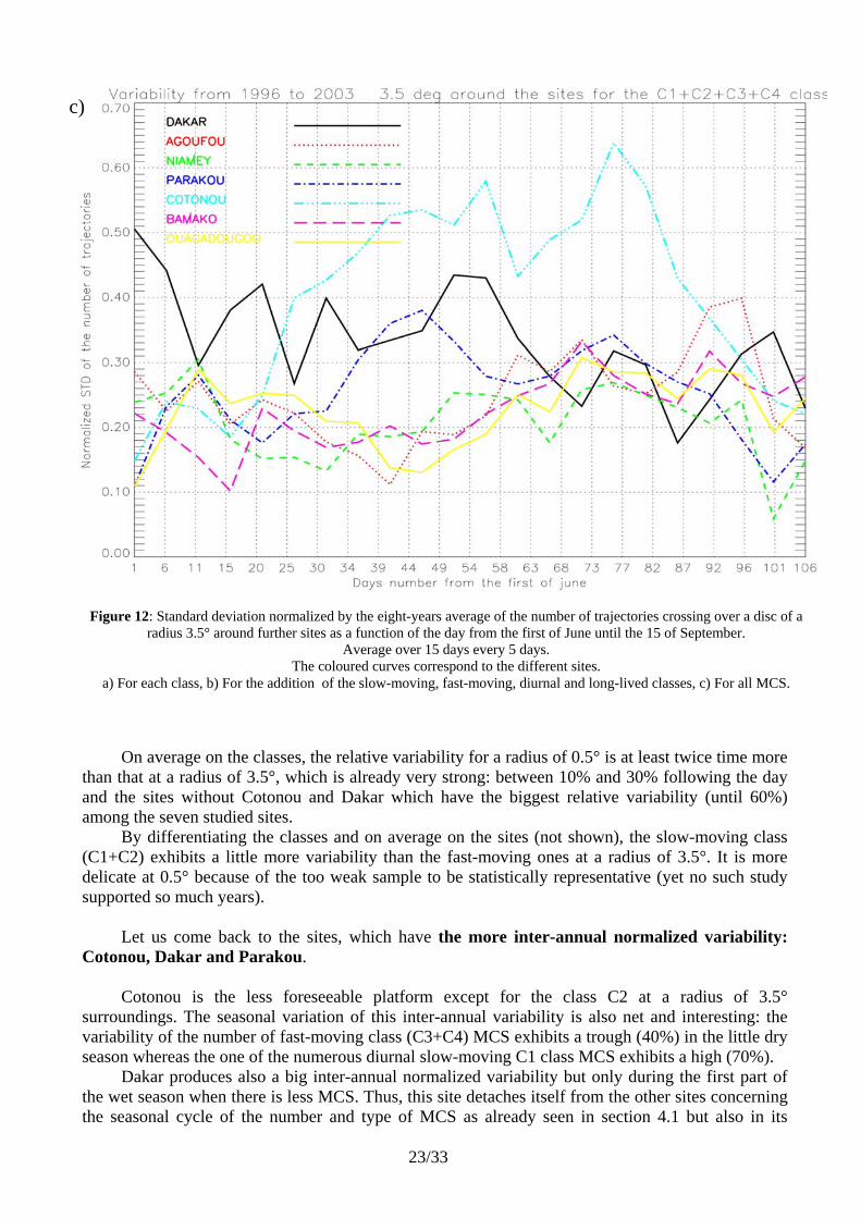
23/33

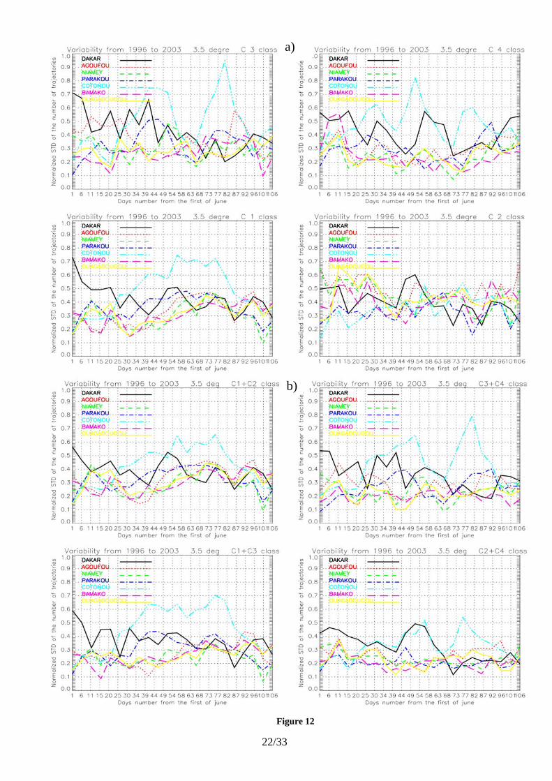
On average on the classes, the relative variability for a radius of 0.5° is at least twice time more than that at a radius of 3.5°, which is already very strong: between 10% and 30% following the day and the sites without Cotonou and Dakar which have the biggest relative variability (until 60%) among the seven studied sites.

By differentiating the classes and on average on the sites (not shown), the slow-moving class (C1+C2) exhibits a little more variability than the fast-moving ones at a radius of 3.5°. It is more delicate at 0.5° because of the too weak sample to be statistically representative (yet no such study supported so much years).

Let us come back to the sites, which have the more inter-annual normalized variability:

Cotonou, Dakar and Parakou. Cotonou is the less foreseeable platform except for the class C2 at a radius of 3.5°

surroundings. The seasonal variation of this inter-annual variability is also net and interesting: the variability of the number of fast-moving class (C3+C4) MCS exhibits a trough (40%) in the little dry season whereas the one of the numerous diurnal slow-moving C1 class MCS exhibits a high (70%).

Dakar produces also a big inter-annual normalized variability but only during the first part of the wet season when there is less MCS. Thus, this site detaches itself from the other sites concerning the seasonal cycle of the number and type of MCS as already seen in section 4.1 but also in its

c)

Figure 12: Standard deviation normalized by the eight-years average of the number of trajectories crossing over a disc of a radius 3.5° around further sites as a function of the day from the first of June until the 15 of September.

Average over 15 days every 5 days. The coloured curves correspond to the different sites.

a) For each class, b) For the addition of the slow-moving, fast-moving, diurnal and long-lived classes, c) For all MCS.

24/33

variability. But be careful, because we divide the standard deviation by the number of events so that a few number increases mathematically the variability, which is the case for Dakar.

Parakou, which is after Cotonou the more southern site, exhibits the same behaviour than Cotonou except for the disc of 0.5°. Indeed, the MCS crossing the south of Parakou must transmit their characters due to their number. An interesting work should be to understand those differences between the more southern sites and others, by comparing the variability in the Guinean Gulf of the sea surface temperatures, or the winds …

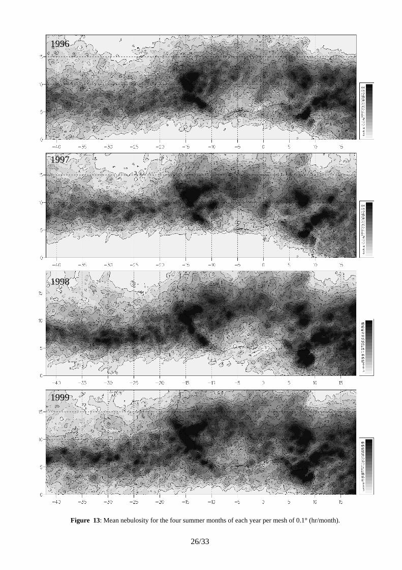
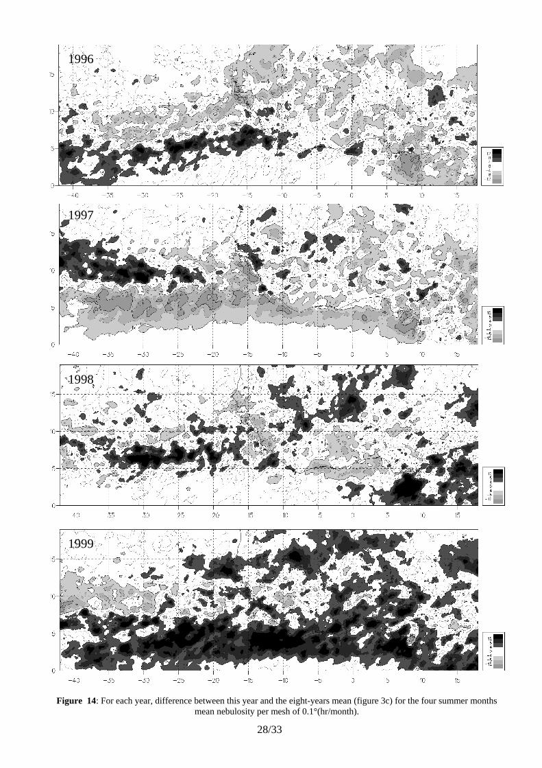
For each year, the geographical repartition of the nebulosity is given figure 13 and the

deviation to the eight-year average Figure 14. Files 20 and 21 show the same parameters respectively but per class. It confirms the conclusions drawn in section 4.1 about the seasonal cycle of the different years and sites. Indeed, the year:

• 1999 is quite wet as compared to the eight-years average, particularly towards the south where the systems are smaller as we have seen within the classification section 3.2 but also for the C4 class.

• 2001 is confirmed as a dry year, except for Dakar (due to the C4 class), the sahelean band between 14°N and 18°N and the continent between 10°W and 5°E.

It also proved the dryness of the year 1997 but also 1996, 2000, with less cloud coverage by the C4 class, and 2002 over the Atlantic ocean.

Over the EPSAT7-Niger zone Laurent et al. (1998a) noticed that the inter-annual variability of the rainfall was due to the variability in the number of MCS.

4.3 Diurnal cycle On the request of the aircraft operators of the Special Observation Period (SOP), the MCS

diurnal cycle is precised around the sites (and not above a point like classical studies) where flights will occur.

The diurnal cycle of the initiations, dissipations, cloud covers and precipitations differs

following the convection types, the regions (ocean, vegetation, orography, …), the atmospheric waves.

Over ocean, diurnal cycle of MCS is complex and not completely understood. It depends on their vertical and horizontal extend. Chen et al. (1996), who have classified the 208 K cloud clusters of the oceanic COARE region following their size, conclude to a weak diurnal cycle for the smallest clouds but to a strong amplitude for the biggest ones. On a largest area, the tropical Pacific ocean, Mapes and Houze (1993) precise the MCS cycles:

• the coldest and largest (208 K, area > 640000 km²) have a strong diurnal cycle with a maximum in the early morning and a minimum in the afternoon.

• the warmest (235 K) or the smallest (area < 250000 km²) are sun-synchronous. Machado et al. (1993), on the East tropical Atlantic, arrived to the same conclusion with a

study on the temperature only. On the contrary, over the continents, Laurent (2005) and Mathon (2001) showed a maximum of

initiations and of cloud coverage (at 235 K) during the afternoon. Yet, this maximum occurs 2 to 4 hours earlier on the amazonian zone than on the sahelean zone. The difference in the precipitation is more fundamental: On the Amazonia, its maximum happens between the maxima of initiations and cloud cover while on the Sahel, it happens at the end of the night and during the morning, because the Sahelean rainfalls are mostly provided by long-lived systems born more eastwards several hours earlier.

On the central Sahel, Machado et al. (1993) had already concluded to the large diurnal amplitude of the convective activity of the coldest clusters (< 253 K). But all clusters gave a nebulosity maximum in the late afternoon and minimum at noon.

From Mathon and Laurent (2001), the Epsat-Sahel zone gives birth to long-lived MCS (> 24 hours) around 1400 LST against 1600 LST for the shortest ones (< 10 hours), and that whatever the

25/33

brightness temperature. The peak of nebulosity occurs three hours later after development and aggregation. The short-lived cells vanish or merge with the largest MCS until morning. The cloud coverage is modulated by the number of short-lived systems and by the size of long-lived ones.

Our results confirm the conclusions of the preceding authors on continents with a maximum of

clouds initiations in the afternoon and a minimum at the end of the morning, all merged classes but apart Dakar where the diurnal cycle stays weak.

Indeed, the files 13 to 19 show the diurnal cycle of the number of trajectories being born and entered in the disc of radius 3.5° around some sites or having disappeared and left this disc, with the following details:

• Like Mathon and Laurent (2001), who separate the cold clusters (213 K to 253 K) into two classes of duration (threshold at 24 hours), our long-lived trajectories (threshold at 9 hours) have a weaker diurnal cycle than the short ones. The central Sahel long-lived MCS of those authors have a diurnal cycle of very weak amplitude. Our long-lived clusters diurnal cycle amplitude (C2+C4) is two times smaller than the one of short-lived clusters (C1+C3) on approximatively the same area (figure 15 for Niamey). But by going towards the south the long-lived MCS cycle weakens until being inexistant around Cotonou (file 15).

• The initiation curve is a bit delated (1.5 hours) with the latitude from Cotonou to Agoufou.

• The dissipation curve has an amplitude maximum in the first part of the night for the classes of trajectories which have a real cycle (short-lived classes C1 and C3) because the squall line class has no dissipation cycle.

V Conclusion Eight summers of infrared satellite data issued from the convective clouds tracking software of

Météo-France over West Africa have been treated. A classification in four classes of the MCS as a function of their speed and lifetime has been

proposed in order to simplify and unify observations, scientific discussions and results. Together with their climatology (number, nebulosity, size, diurnal, seasonal and inter-annual variation, spatial distribution versus the four classes) on several supersites of observations (Agoufou, Bamako, Cotonou, Dakar, Niamey, Ouadagoudou, Parakou), it will help the SOP planning and operations during summer 2006.

Obviously, no relation with the precipitation has been directly made in our work. Nevertheless, further studies have shown the good correlation between the rain core and the coldest core in term of brightness temperature (See Laurent et al. 1998b for a review of the existing methods on ground rainfall estimated by satellite). The Tropical Rainfall Measuring Mission (TRMM) and the EPSAT7-Niger network have had the purpose to find a correlation between rainfall and satellite measurements. According to Jobard and Desbois (1992), correlation between precipitation and satellite coverage is valid on spatio-temporal mean only. Over TOGA-COARE area, Rickenbach (1999) showed also that the propagation of satellite observed cold cloud shield can be decoupled from the propagation of the underlying squall line observed from radar network. Moreover, evaporation of the precipitation before it reaches the ground is another difficulty!

Other studies are imaginable with our eight years MCS characteristics and trajectories data base like the geographical repartition of the initiations and dissipations, the trajectories as a function of the region, orography, winds, period …, or the MCS morphology versus the different classes, the relation with the atmospheric and surface conditions… As a consequence, the data are available for the AMMA community under the form of ASCII files (see an extract file 1), explained file 2 and readable with the FORTRAN 90 file3.

26/33

1996

1997

1998

1999

Figure 13: Mean nebulosity for the four summer months of each year per mesh of 0.1° (hr/month).

27/33

2001

2002

2003

Figure 13

2000

28/33

1996

1997

1998

1999

Figure 14: For each year, difference between this year and the eight-years mean (figure 3c) for the four summer months mean nebulosity per mesh of 0.1°(hr/month).

29/33

2001

2002

2003

Figure 14

2000

30/33

Figure 15: Eight years average diurnal cycle of the number of MCS trajectories in the disc of a radius 3.5° around NIAMEY. The black unbroken curve

corresponds to the MCS births or entries in the disc. The red broken line corresponds to the collapses or exits. Hours in Universal Time. a) For each class, b) For the addition of the diurnal and long-lived classes,

c) For all MCS. See files 13 to 19 for all platforms.

The every 30 mn fluctuations, corresponding to the temporal discretisation, are due to the lack of data.

The trajectories during less than 1 hour (that is to say during 30 mn) have been eliminated.

b)

c)

a)

31/33

VI Reference Arnaud Y., Desbois M. and Maizi J., 1992, Automatic tracking and characterization of African

convective systems on Meteosat pictures, J. of Applied Met., vol. 31, p443-453. Barnes G. and Sieckman K., 1984, The environment of fast- and slow-moving tropical mesoscale

convective cloud lines, Mon. Wea. Rev., 112, p1782-1794. Chen S., Houze R. and Mapes B., 1996, Multiscale variability of deep convection in relation to

large-scale circulation in TOGA COARE, J. of atm. Sc., vol. 53, n°10, p1380-1409. Jobard I. and Desbois M., 1992, Remote sensing of rainfall over the tropical Africa using

METEOSAT infrared imagery, Int. Remote Sensing, 13-14, p2683-2700. Lafore J-P. and Moncrieff M., 1989, A numerical investigation of the organization and

interaction of the convective and stratiform regions of tropical squall lines, J. of atm. Sc., 45, p521-544.

Laurent H., 2005, Contribution à l’étude des systèmes convectifs en régions tropicales, HDR.,

University of Grenoble I, France. Laurent H., D'Amato N. and Lebel T., 1998a, How important is the contribution of the

Mesoscale Convective Complexes to the Sahelian rainfall?, Phys. Chem. Earth, 23, p629-633.

Laurent H., Jobard I. and Toma A., 1998b, Validation of satellite and ground-based estimates of

precipitation over the Sahel, Atm. Research, 47-48, p651-670. Laurent H., Machado L., Morales C. and Durieux L., 2002, Characteristics of the Amazonian

mesoscale convective systems observed from satellite and radar during the WETAMC/LBA experiment, J. Geophys. Res., 107 (D18), 8054, doi:10.1029/2001JD000337.

Machado L., Desbois M. and Duvel J-P., 1992, Structural characteristics of deep convective

systems over Tropical Africa and the Atlantic Ocean, Mon. weather rev., 120, p392-406. Machado L., Duvel J-P. and Desbois M., 1993, Diurnal variations and modulation of easterly

waves on the size distribution of the convective cloud clusters over the West Africa and the Atlantic Ocean, Mon. weather rev., 121, p37-49.

Maddox R., 1980, Mesoscale convective complexes, Bull. Amer. Met. Soc., 61, p1374-1387. Mapes B. and Houze R., 1993, Cloud clusters and superclusters over the oceanic warm pool,

Mon. Wea. Rev., 121, p1398-1415. Mathon V., 2001, Etude climatologique des systèmes convectifs de méso-échelle en Afrique de

l’Ouest, PhD, University of Paris VII. Mathon V. and Laurent H., 2001, Life cycle of Sahelian mesoscale convective cloud systems, Q.

J. R. M. Soc., 127, p377-406. Mathon V., Laurent H. and Lebel T., 2002, Mesoscale convective systems in the Sahel, J. of

Applied Met., vol. 41, n°11, p1081-1092.

32/33

Morel C. and Sénési S., 2002, A climatology of mesoscale convective systems over Europe using

satellite infrared imagery. I: Methodology, Q. J. R. M. Soc., 128, p1953-1992. Rickenbach T., 1999, Cloud-top evolution of tropical oceanic squall lines from radar reflectivity

and infrared satellite data, Mon. Wea. Rev., 127, p2951-2976. Roca R., Lafore JP., Piriou C. and Redelsperger JL., 2005, Extratropical Dry-Air Intrusions

into the West African Monsoon Midtroposphere: An Important Factor for the Convective Activity over the Sahel, J. Atmos. Sci., 62, n°2, p390-407.

Rotunno, R, Klemp J. B. and Weisman M. L., 1988, A theory for strong, long-lived squall lines,

J. Atmos. Sci., 45, p463-485. Williams M. and Houze R., 1987, Satellite observed characteristics of winter monsoon cloud

clusters, Mon. Wea. Rev., 115, p505-519.

33/33

VII List of external files File 1: Example of an ASCII outfile of the RDT software in its climatological version. The

trajectories of the MCS and the cells that have composed them are described. File 2: Description file of an ASCII outfile of the RDT software in its climatological version. File 3: Fortran 90 file to read data of an ASCII outfile of the RDT software in its climatological

version. File 4: Number of trajectories per day crossing over a disc of a radius 3.5° around AGOUFOU as a

function of the day from the first of June until the 15 of September. Average over 15 days every 5 days.

The coloured curves correspond to the 8 years. Their average and standard deviation are in black.

a) For each class, b) For the classes summation two by two, c) For all MCS. File 5: The same as File 4 but for BAMAKO. File 6: The same as File 4 but for COTONOU. File 7: The same as File 4 but for DAKAR. File 8: The same as File 4 but for NIAMEY. File 9: The same as File 4 but for OUADAGOUDOU. File 10: The same as File 4 but for PARAKOU. File 11: Average on the 8 years of the number of trajectories per day crossing over a disc of a radius

0.5° around further sites as a function of the day from the first of June until the 15 of September. Average over 15 days every 5 days.

The coloured curves correspond to the different sites. a) For each class, b) For the addition of the slow-moving, fast-moving, diurnal and long-lived

classes, c) For all MCS. File 12: Standard deviation normalized by the 8 years average of the number of trajectories crossing

over a disc of a radius 0.5° around further sites as a function of the day from the first of June until the 15 of September. Average over 15 days every 5 days.

The coloured curves correspond to the different sites. a) For each class (some data are missing for Cotonou because one divides by a zero eight-

years average: there is no trajectory on average on 15 days the days 60 for the C1 class, 65 to 75 for C2 and 65 for C3), b) For the addition of the slow-moving, fast-moving, diurnal and long-lived classes, c) For all MCS.

File 13: Eight years average diurnal cycle of the number of MCS trajectories in the disc of a radius 3.5° around AGOUFOU. The black unbroken curve corresponds to the MCS births or entries in the disc. The red broken line corresponds to the collapses or outflows. The trajectories during less than 1 hour (that is to say during 30 mn) have been eliminated.

a) For each class, b) For the addition of the slow-moving, fast-moving, diurnal and long-lived classes, c) For all MCS.

File 14: The same as file 13 but for BAMAKO. File 15: The same as file 13 but for COTONOU. File 16: The same as file 13 but for DAKAR. File 17: The same as file 13 but for NIAMEY. File 18: The same as file 13 but for OUADAGOUDOU. File 19: The same as file 13 but for PARAKOU. File 20: Four summer months mean nebulosity for each year and each class per mesh of 0.1°

(hr/month). File 21: Deviation from the average nebulosity of the four summer months of the eight-years for

each class (this average is shown figure 3a) for each year and each class per mesh of 0.1° (hr/month).