Embed Size (px)
Citation preview

Programming in
Martin-Lof’s Type Theory
An Introduction
Bengt Nordstrom
Kent Petersson
Jan M. Smith
Department of Computing SciencesUniversity of Goteborg / Chalmers
S-412 96 GoteborgSweden
This book was published by Oxford University Press in 1990. It is now out ofprint. This version is available from www.cs.chalmers.se/Cs/Research/Logic.

ii

iii
Preface
It is now 10 years ago that two of us took the train to Stockholm to meetPer Martin-Lof and discuss his ideas on the connection between type theoryand computing science. This book describes different type theories (theoriesof types, polymorphic and monomorphic sets, and subsets) from a computingscience perspective. It is intended for researchers and graduate students withan interest in the foundations of computing science, and it is mathematicallyself-contained.
We started writing this book about six years ago. One reason for this longtime is that our increasing experience in using type theory has made severalchanges of the theory necessary. We are still in this process, but have neverthe-less decided to publish the book now.
We are, of course, greatly indebted to Per Martin-Lof; not only for creatingthe subject of this book, but also for all the discussions we have had with him.Beside Martin-Lof, we have discussed type theory with many people and wein particular want to thank Samson Abramsky, Peter Aczel, Stuart Anderson,Roland Backhouse, Bror Bjerner, Robert Constable, Thierry Coquand, PeterDybjer, Roy Dyckhoff, Gerard Huet, Larry Paulson, Christine Paulin-Mohring,Anne Salvesen, Bjorn von Sydow, and Dan Synek. Thanks to Dan Synek alsofor his co-authorship of the report which the chapter on trees is based on.
Finally, we would like to thank STU, the National Swedish Board For Tech-nical Development, for financial support.
Bengt Nordstrom, Kent Petersson and Jan Smith
Goteborg, Midsummer Day 1989.

iv

Contents
1 Introduction 11.1 Using type theory for programming . . . . . . . . . . . . . . . . . 31.2 Constructive mathematics . . . . . . . . . . . . . . . . . . . . . . 61.3 Different formulations of type theory . . . . . . . . . . . . . . . . 61.4 Implementations of programming logics . . . . . . . . . . . . . . 8
2 The identification of sets, propositions and specifications 92.1 Propositions as sets . . . . . . . . . . . . . . . . . . . . . . . . . . 92.2 Propositions as tasks and specifications of programs . . . . . . . 12
3 Expressions and definitional equality 133.1 Application . . . . . . . . . . . . . . . . . . . . . . . . . . . . . . 133.2 Abstraction . . . . . . . . . . . . . . . . . . . . . . . . . . . . . . 143.3 Combination . . . . . . . . . . . . . . . . . . . . . . . . . . . . . 153.4 Selection . . . . . . . . . . . . . . . . . . . . . . . . . . . . . . . . 163.5 Combinations with named components . . . . . . . . . . . . . . . 163.6 Arities . . . . . . . . . . . . . . . . . . . . . . . . . . . . . . . . . 173.7 Definitions . . . . . . . . . . . . . . . . . . . . . . . . . . . . . . . 193.8 Definition of what an expression of a certain arity is . . . . . . . 193.9 Definition of equality between two expressions . . . . . . . . . . . 20
I Polymorphic sets 23
4 The semantics of the judgement forms 254.1 Categorical judgements . . . . . . . . . . . . . . . . . . . . . . . 27
4.1.1 What does it mean to be a set? . . . . . . . . . . . . . . . 274.1.2 What does it mean for two sets to be equal? . . . . . . . 284.1.3 What does it mean to be an element in a set? . . . . . . . 284.1.4 What does it mean for two elements to be equal in a set? 294.1.5 What does it mean to be a proposition? . . . . . . . . . . 294.1.6 What does it mean for a proposition to be true? . . . . . 29
4.2 Hypothetical judgements with one assumption . . . . . . . . . . 294.2.1 What does it mean to be a set under an assumption? . . 304.2.2 What does it mean for two sets to be equal under an
assumption? . . . . . . . . . . . . . . . . . . . . . . . . . . 304.2.3 What does it mean to be an element in a set under an
assumption? . . . . . . . . . . . . . . . . . . . . . . . . . . 30
v

vi CONTENTS
4.2.4 What does it mean for two elements to be equal in a setunder an assumption? . . . . . . . . . . . . . . . . . . . . 31
4.2.5 What does it mean to be a proposition under an assumption? 314.2.6 What does it mean for a proposition to be true under an
assumption? . . . . . . . . . . . . . . . . . . . . . . . . . . 314.3 Hypothetical judgements with several assumptions . . . . . . . . 31
4.3.1 What does it mean to be a set under several assumptions? 314.3.2 What does it mean for two sets to be equal under several
assumptions? . . . . . . . . . . . . . . . . . . . . . . . . . 324.3.3 What does it mean to be an element in a set under several
assumptions? . . . . . . . . . . . . . . . . . . . . . . . . . 324.3.4 What does it mean for two elements to be equal in a set
under several assumptions? . . . . . . . . . . . . . . . . . 334.3.5 What does it mean to be a proposition under several as-
sumptions? . . . . . . . . . . . . . . . . . . . . . . . . . . 334.3.6 What does it mean for a proposition to be true under
several assumptions? . . . . . . . . . . . . . . . . . . . . . 33
5 General rules 355.1 Assumptions . . . . . . . . . . . . . . . . . . . . . . . . . . . . . 375.2 Propositions as sets . . . . . . . . . . . . . . . . . . . . . . . . . . 375.3 Equality rules . . . . . . . . . . . . . . . . . . . . . . . . . . . . . 375.4 Set rules . . . . . . . . . . . . . . . . . . . . . . . . . . . . . . . . 385.5 Substitution rules . . . . . . . . . . . . . . . . . . . . . . . . . . . 38
6 Enumeration sets 416.1 Absurdity and the empty set . . . . . . . . . . . . . . . . . . . . 436.2 The one-element set and the true proposition . . . . . . . . . . . 436.3 The set Bool . . . . . . . . . . . . . . . . . . . . . . . . . . . . . 44
7 Cartesian product of a family of sets 477.1 The formal rules and their justification . . . . . . . . . . . . . . . 497.2 An alternative primitive non-canonical form . . . . . . . . . . . . 517.3 Constants defined in terms of the Π set . . . . . . . . . . . . . . 53
7.3.1 The universal quantifier ( ∀) . . . . . . . . . . . . . . . . . 537.3.2 The function set (→) . . . . . . . . . . . . . . . . . . . . . 537.3.3 Implication (⊃ ) . . . . . . . . . . . . . . . . . . . . . . . 54
8 Equality sets 578.1 Intensional equality . . . . . . . . . . . . . . . . . . . . . . . . . . 578.2 Extensional equality . . . . . . . . . . . . . . . . . . . . . . . . . 608.3 η-equality for elements in a Π set . . . . . . . . . . . . . . . . . . 62
9 Natural numbers 63
10 Lists 67
11 Cartesian product of two sets 7311.1 The formal rules . . . . . . . . . . . . . . . . . . . . . . . . . . . 7311.2 Extensional equality on functions . . . . . . . . . . . . . . . . . . 76

CONTENTS vii
12 Disjoint union of two sets 79
13 Disjoint union of a family of sets 81
14 The set of small sets (The first universe) 8314.1 Formal rules . . . . . . . . . . . . . . . . . . . . . . . . . . . . . . 8314.2 Elimination rule . . . . . . . . . . . . . . . . . . . . . . . . . . . 91
15 Well-orderings 9715.1 Representing inductively defined sets by well-orderings . . . . . . 101
16 General trees 10316.1 Formal rules . . . . . . . . . . . . . . . . . . . . . . . . . . . . . . 10416.2 Relation to the well-order set constructor . . . . . . . . . . . . . 10616.3 A variant of the tree set constructor . . . . . . . . . . . . . . . . 10816.4 Examples of different tree sets . . . . . . . . . . . . . . . . . . . . 108
16.4.1 Even and odd numbers . . . . . . . . . . . . . . . . . . . 10816.4.2 An infinite family of sets . . . . . . . . . . . . . . . . . . . 110
II Subsets 111
17 Subsets in the basic set theory 113
18 The subset theory 11718.1 Judgements without assumptions . . . . . . . . . . . . . . . . . . 117
18.1.1 What does it mean to be a set? . . . . . . . . . . . . . . . 11818.1.2 What does it mean for two sets to be equal? . . . . . . . 11818.1.3 What does it mean to be an element in a set? . . . . . . . 11818.1.4 What does it mean for two elements to be equal in a set? 11918.1.5 What does it mean to be a proposition? . . . . . . . . . . 11918.1.6 What does it mean for a proposition to be true? . . . . . 119
18.2 Hypothetical judgements . . . . . . . . . . . . . . . . . . . . . . . 11918.2.1 What does it mean to be a set under assumptions? . . . 12018.2.2 What does it mean for two sets to be equal under assump-
tions? . . . . . . . . . . . . . . . . . . . . . . . . . . . . . 12018.2.3 What does it mean to be an element in a set under as-
sumptions? . . . . . . . . . . . . . . . . . . . . . . . . . . 12118.2.4 What does it mean for two elements to be equal in a set
under assumptions? . . . . . . . . . . . . . . . . . . . . . 12118.2.5 What does it mean to be a proposition under assumptions?12218.2.6 What does it mean for a proposition to be true under
assumptions? . . . . . . . . . . . . . . . . . . . . . . . . . 12218.3 General rules in the subset theory . . . . . . . . . . . . . . . . . 12218.4 The propositional constants in the subset theory . . . . . . . . . 124
18.4.1 The logical constants . . . . . . . . . . . . . . . . . . . . . 12418.4.2 The propositional equality . . . . . . . . . . . . . . . . . . 125
18.5 Subsets formed by comprehension . . . . . . . . . . . . . . . . . . 12618.6 The individual set formers in the subset theory . . . . . . . . . . 127
18.6.1 Enumeration sets . . . . . . . . . . . . . . . . . . . . . . . 12718.6.2 Equality sets . . . . . . . . . . . . . . . . . . . . . . . . . 127

viii CONTENTS
18.6.3 Natural numbers . . . . . . . . . . . . . . . . . . . . . . . 12818.6.4 Cartesian product of a family of sets . . . . . . . . . . . . 12818.6.5 Disjoint union of two sets . . . . . . . . . . . . . . . . . . 13018.6.6 Disjoint union of a family of sets . . . . . . . . . . . . . . 13018.6.7 Lists . . . . . . . . . . . . . . . . . . . . . . . . . . . . . . 13118.6.8 Well-orderings . . . . . . . . . . . . . . . . . . . . . . . . 131
18.7 Subsets with a universe . . . . . . . . . . . . . . . . . . . . . . . 131
III Monomorphic sets 135
19 Types 13719.1 Types and objects . . . . . . . . . . . . . . . . . . . . . . . . . . 13819.2 The types of sets and elements . . . . . . . . . . . . . . . . . . . 13919.3 Families of types . . . . . . . . . . . . . . . . . . . . . . . . . . . 13919.4 General rules . . . . . . . . . . . . . . . . . . . . . . . . . . . . . 14119.5 Assumptions . . . . . . . . . . . . . . . . . . . . . . . . . . . . . 14219.6 Function types . . . . . . . . . . . . . . . . . . . . . . . . . . . . 143
20 Defining sets in terms of types 14720.1 Π sets . . . . . . . . . . . . . . . . . . . . . . . . . . . . . . . . . 14820.2 Σ sets . . . . . . . . . . . . . . . . . . . . . . . . . . . . . . . . . 14920.3 Disjoint union . . . . . . . . . . . . . . . . . . . . . . . . . . . . . 15020.4 Equality sets . . . . . . . . . . . . . . . . . . . . . . . . . . . . . 15020.5 Finite sets . . . . . . . . . . . . . . . . . . . . . . . . . . . . . . . 15120.6 Natural numbers . . . . . . . . . . . . . . . . . . . . . . . . . . . 15120.7 Lists . . . . . . . . . . . . . . . . . . . . . . . . . . . . . . . . . . 152
IV Examples 153
21 Some small examples 15521.1 Division by 2 . . . . . . . . . . . . . . . . . . . . . . . . . . . . . 15521.2 Even or odd . . . . . . . . . . . . . . . . . . . . . . . . . . . . . . 15921.3 Bool has only the elements true and false . . . . . . . . . . . . . . 16021.4 Decidable predicates . . . . . . . . . . . . . . . . . . . . . . . . . 16221.5 Stronger elimination rules . . . . . . . . . . . . . . . . . . . . . . 163
22 Program derivation 16722.1 The program derivation method . . . . . . . . . . . . . . . . . . . 167
22.1.1 Basic tactics . . . . . . . . . . . . . . . . . . . . . . . . . 16822.1.2 Derived tactics . . . . . . . . . . . . . . . . . . . . . . . . 170
22.2 A partitioning problem . . . . . . . . . . . . . . . . . . . . . . . . 171
23 Specification of abstract data types 17923.1 Parameterized modules . . . . . . . . . . . . . . . . . . . . . . . . 18123.2 A module for sets with a computable equality . . . . . . . . . . . 182
A Constants and their arities 197A.1 Primitive constants in the set theory . . . . . . . . . . . . . . . . 197A.2 Set constants . . . . . . . . . . . . . . . . . . . . . . . . . . . . . 198

CONTENTS ix
B Operational semantics 199B.1 Evaluation rules for noncanonical constants . . . . . . . . . . . . 200

x CONTENTS

Chapter 1
Introduction
In recent years several formalisms for program construction have been intro-duced. One such formalism is the type theory developed by Per Martin-Lof. Itis well suited as a theory for program construction since it is possible to expressboth specifications and programs within the same formalism. Furthermore, theproof rules can be used to derive a correct program from a specification as wellas to verify that a given program has a certain property. This book contains anintroduction to type theory as a theory for program construction.
As a programming language, type theory is similar to typed functional lan-guages such as Hope [18] and ML [44], but a major difference is that the evalua-tion of a well-typed program always terminates. In type theory it is also possibleto write specifications of programming tasks as well as to develop provably cor-rect programs. Type theory is therefore more than a programming language andit should not be compared with programming languages, but with formalizedprogramming logics such as LCF [44] and PL/CV [24].
Type theory was originally developed with the aim of being a clarification ofconstructive mathematics, but unlike most other formalizations of mathematicstype theory is not based on first order predicate logic. Instead, predicate logicis interpreted within type theory through the correspondence between propo-sitions and sets [28, 52]. A proposition is interpreted as a set whose elementsrepresent the proofs of the proposition. Hence, a false proposition is interpretedas the empty set and a true proposition as a non-empty set. Chapter 2 containsa detailed explanation of how the logical constants correspond to sets, thus ex-plaining how a proposition could be interpreted as a set. A set cannot only beviewed as a proposition; it is also possible to see a set as a problem description.This possibility is important for programming, because if a set can be seen asa description of a problem, it can, in particular, be used as a specification of aprogramming problem. When a set is seen as a problem, the elements of the setare the possible solutions to the problem; or similarly if we see the set as a spec-ification, the elements are the programs that satisfy the specification. Hence,set membership and program correctness are the same problem in type theory,and because all programs terminate, correctness means total correctness.
One of the main differences between the type theory presentation in thisbook and the one in [69] is that we use a uniform notation for expressions.Per Martin-Lof has formulated a theory of mathematical expressions in general,which is presented in chapter 3. We describe how arbitrary mathematical ex-
1

2 CHAPTER 1. INTRODUCTION
pressions are formed and introduce an equality between expressions. We alsoshow how defined constants can be introduced as abbreviations of more compli-cated expressions.
In Part I we introduce a polymorphic version of type theory. This version isthe same as the one presented by Martin-Lof in Hannover 1979 [69] and in hisbook Intuitionistic Type Theory [70] except that we use an intensional versionof the equality.
Type theory contains rules for making judgements of the following fourforms:
A is a setA1 and A2 are equal setsa is an element in the set Aa1 and a2 are equal elements in the set A
The semantics of type theory explains what judgements of these forms mean.Since the meaning is explained in a manner quite different from that which iscustomary in computer science, let us first describe the context in which themeaning is explained. When defining a programming language, one often ex-plains its notions in terms of mathematical objects like sets and functions. Sucha definition takes for granted the existence and understanding of these objects.Since type theory is intended to be a fundamental conceptual framework for thebasic notions of constructive mathematics, it is infeasible to explain the mean-ing of type theory in terms of some other mathematical theory. The meaning oftype theory is explained in terms of computations. The first step in this processis to define the syntax of programs and how they are computed. We first intro-duce the canonical expressions which are the expressions that can be the resultof programs. When they are defined, it is possible to explain the judgements,first the assumption-free and then the hypothetical. A set is explained in termsof canonical objects and their equality relation, and when the notion of set isunderstood, the remaining judgement forms are explained. Chapter 4 containsa complete description of the semantics in this manner.
The semantics of the judgement forms justifies a collection of general rulesabout assumptions, equality and substitution which is presented in chapter 5.
In the following chapters (7 – 17), we introduce a collection of sets andset forming operations suitable both for mathematics and computer science.Together with the sets, the primitive constants and their computation rules areintroduced. We also give the rules of a formal system for type theory. The rulesare formulated in the style of Gentzen’s natural deduction system for predicatelogic and are justified from
• the semantic explanations of the judgement forms,
• the definitions of the sets, and
• the computation rules of the constants.
We do not, however, present justifications of all rules, since many of the justifi-cations follow the same pattern.
There is a major disadvantage with the set forming operations presentedin part I because programs sometimes will contain computationally irrelevantparts. In order to remedy this problem we will in part II introduce rules which

1.1. USING TYPE THEORY FOR PROGRAMMING 3
makes it possible to form subsets. However, if we introduce subsets in thesame way as we introduced the other set forming operations, we cannot justifya satisfactory elimination rule. Therefore, we define a new theory, the subsettheory, and explain the judgements in this new theory by translating them intojudgements in the basic theory, which we already have given meaning to in partI.
In part III, we briefly describe a theory of types and show how it can beused as an alternative way of providing meaning to the judgement forms intype theory. The origin of the ideas in this chapter is Martin-Lof’s analysisof the notions of proposition, judgement and proof in [71]. The extension oftype theory presented is important since it makes it possible to introduce moregeneral assumptions within the given formalism. We also show how the theoryof types could be used as a framework for defining some of the sets which wereintroduced in part I.
In part IV we present some examples from logic and programming. Weshow how type theory can be used to prove properties of programs and alsohow to formally derive programs for given specifications. Finally we describehow abstract data types can be specified and implemented in type theory.
1.1 Using type theory for programming
Type theory, as it is used in this book, is intended as a theory for programconstruction. The programming development process starts with the task ofthe program. Often, this is just existing in the head of the programmer, butit can also exist explicitly as a specification that expresses what the programis supposed to do. The programmer, then, either directly writes down a pro-gram and proves that it satisfies the given specification, or successively derivesa program from the specification. The first method is called program verifica-tion and the second program derivation . Type theory supports both methodsand it is assumed that it is the programmer who bridges the gap between thespecification and the program.
There are many examples of correctness proofs in the literature and proofsdone in Martin-Lof’s type theory can be found in [20, 75, 82]. A theory whichis similar to type theory is Huet and Coquand’s Calculus of Constructions [27]and examples of correctness proofs in this theory can be found in [74].
There are fewer examples of formal program derivations in the literature.Manna and Waldinger have shown how to derive a unification algorithm usingtheir tableau method [63] and there are examples developed in Martin-Lof’stype theory in Backhouse et al [6] and in the Theory of Constructions in Paulin-Mohring [80]. A formal derivation of the partitioning problem using type theoryis presented in [87]; a slightly changed version of this derivation is also presentedin chapter 22.
In the process of formal program development, there are two different stagesand usually two different languages involved. First, we have the specificationprocess and the specification language, and then the programming process andthe programming language. The specification process is the activity of find-ing and formulating the problem which the program is to solve. This processis not dealt with in this book. We assume that the programmer knows whatproblem to solve and is able to express it as a specification. A specification is

4 CHAPTER 1. INTRODUCTION
in type theory expressed as a set, the set of all correct programs satisfying thespecification. The programming process is the activity of finding and formu-lating a program which satisfies the specification. In type theory, this meansthat the programmer constructs an element in the set which is expressed by thespecification. The programs are expressed in a language which is a functionalprogramming language. So it is a programming language without assignmentsand other side effects. The process of finding a program satisfying a specifica-tion can be formalized in a programming logic, which has rules for deducingthe correctness of programs. So the formal language of type theory is used as aprogramming language, a specification language and a programming logic.
The language for sets in type theory is similar to the type system in program-ming languages except that the language is much more expressive. Besides theusual set forming operations which are found in type systems of programminglanguages (Bool, A+B, A → B, A×B, List(A), etc.) there are operations whichmake it possible to express properties of programs using the usual connectivesin predicate logic. It is possible to write down a specification without knowingif there is a program satisfying it. Consider for example
(∃a ∈ N+)(∃b ∈ N+)(∃c ∈ N+)(∃n ∈ N+)(n > 2 & an + bn = cn)
which is a specification of a program which computes four natural numbers suchthat Fermat’s last theorem is false. It is also possible that a specification is sat-isfied by several different programs. Trivial examples of this are “specifications”like N, List(N) → List(N) etc. More important examples are the sorting problem(the order of the elements of the output of a sorting program should not beuniquely determined by the input), compilers (two compilers producing differ-ent code for the same program satisfies the same specification as long as thecode produced computes the correct input-output relation), finding an index ofa maximal element in an array, finding a shortest path in a graph etc.
The language to express the elements in sets in type theory constitutes atyped functional programming language with lazy evaluation order. The pro-gram forming operations are divided into constructors and selectors. Construc-tors are used to construct objects in a set from other objects, examples are 0,succ, pair, inl, inr and λ . Selectors are used as a generalized pattern matching:What in ML is written as
case p of (x,y) => d
is in type theory written assplit(p, (x, y)d)
and if we in ML define the disjoint union by
datatype (’A,’B)Dunion = inl of ’A | inr of ’B
then the ML-expression
case p of inl(x) => d| inr(y) => e
is in type theory written as
when(p, (x)d, (y)e)

1.1. USING TYPE THEORY FOR PROGRAMMING 5
General recursion is not available. Iteration is expressed by using the se-lectors associated with the inductively defined sets like N and List(A). Forthese sets, the selectors work as operators for primitive recursion over the set.For instance, to find a program f(n) on the natural numbers which solves theequations {
f(0) = df(n + 1) = h(n, f(n))
one uses the selector natrec associated with the natural numbers. The equationsare solved by making the definition:
f(n) ≡ natrec(n, d, (x, y)h(x, y))
In order to solve recursive equations which are not primitive recursive, one mustuse the selectors of inductive types together with high order functions. Examplesof how to obtain recursion schemas other than the primitive ones are discussedby Paulson in [84] and Nordstrom [77].
Programs in type theory are computed using lazy evaluation. This meansthat a program is considered to be evaluated if it is on the form
c(e1, . . . , en)
where c is a constructor and e1, . . . , en are expressions. Notice that there is norequirement that the expressions e1, . . . , en must be evaluated. So, for instance,the expression succ(2222
) is considered to be evaluated, although it is not fullyevaluated. If a program is on the form
s(e1, . . . , en)
where s is a selector, it is usually computed by first computing the value of thefirst argument. The constructor of this value is then used to decide which of theremaining arguments of s which is used to compute the value of the expression.
When a user wants to derive a correct program from a specification, she usesa programming logic. The activity to derive a program is similar to provinga theorem in mathematics. In the top-down approach, the programmer startswith the task of the program and divides it into subtasks such that the programssolving the subtasks can be combined into a program for the given task. Forinstance, the problem of finding a program satisfying B can be reduced to findinga program satisfying A and a function taking an arbitrary program satisfyingA to a program satisfying B. Similarly, the mathematician starts with theproposition to be proven and divides it into other propositions such that theproofs of them can be combined into a proof of the proposition. For instance,the proposition B is true if we have proofs of the propositions A and A⊃B.
Type theory is designed to be a logic for mathematical reasoning, and it isthrough the computational content of constructive proofs that it can be usedas a programming logic (by identifying programs and proof objects). So thelogic is rather strong; it is possible to express general mathematical problemsand proofs. This is important for a logic which is intended to work in practice.We want to have a language as powerful as possible to reason about programs.The formal system of type theory is inherently open in that it is possible tointroduce new type forming operations and their rules. The rules have to bejustified using the semantics of type theory.

6 CHAPTER 1. INTRODUCTION
1.2 Constructive mathematics
Constructive mathematics arose as an independent branch of mathematics outof the foundational crisis in the beginning of this century, mainly developed byBrouwer under the name intuitionism. It did not get much support becauseof the general belief that important parts of mathematics were impossible todevelop constructively. By the work of Bishop, however, this belief has beenshown to be wrong. In his book Foundations of Constructive Analysis [10],Bishop rebuilds constructively central parts of classical analysis; and he doesit in a way that demonstrates that constructive mathematics can be as elegantas classical mathematics. Basic information about the fundamental ideas ofintuitionistic mathematics is given in Dummet [33], Heyting [50], and Troelstraand van Dalen [108, 109].
The debate whether mathematics should be built up constructively or notneed not concern us here. It is sufficient to notice that constructive mathematicshas some fundamental notions in common with computer science, above all thenotion of computation. This means that constructive mathematics could be animportant source of inspiration for computer science. This was realized alreadyby Bishop in [11]; Constable made a similar proposal in [23].
The notion of function or method is primitive in constructive mathematicsand a function from a set A to a set B can be viewed as a program which whenapplied to an element in A gives an element in B as output. So all functions inconstructive mathematics are computable. The notion of constructive proof isalso closely related to the notion of computer program. To prove a proposition(∀x∈A)(∃y∈B)P (x, y) constructively means to give a function f which whenapplied to an element a in A gives an element b in B such that P (a, b) holds.So if the proposition (∀x∈A)(∃y∈B)P (x, y) expresses a specification, then thefunction f obtained from the proof is a program satisfying the specification.
A constructive proof could therefore itself be seen as a computer programand the process of computing the value of a program corresponds to the processof normalizing a proof. There is however a small disadvantage of using a con-structive proof as a program because the proof contains a lot of computationallyirrelevant information. To get rid of this information Goto [45], Paulin-Mohring[80], Sato [93], Takasu [106] and Hayashi [49] have developed different tech-niques to synthesize a computer program from a constructive proof; this is alsothe main objective of the subset theory introduced in Part II of this book. Goadhas also used the correspondence between proofs and programs to specialize ageneral program to efficient instantiations [41, 42].
1.3 Different formulations of type theory
One of the basic ideas behind Martin-Lof’s type theory is the Curry-Howardinterpretation of propositions as types, i.e. in our terminology, propositionsas sets. This view of propositions is related both to Heyting’s explanation ofintuitionistic logic [50] and, on a more formal level, to Kleene’s realizabilityinterpretation of intuitionistic arithmetic [59].
Another source for type theory is proof theory. Using the identification ofpropositions and sets, normalizing a derivation is closely related to computingthe value of the proof term corresponding to the derivation. Tait’s computability

1.3. DIFFERENT FORMULATIONS OF TYPE THEORY 7
method [105] from 1967 has been used for proving normalization for many dif-ferent theories; in the Proceedings of the Second Scandinavian Logic Symposium[38] Tait’s method is exploited in papers by Girard, Martin-Lof and Prawitz.One of Martin-Lof’s original aims with type theory was that it could serve asa framework in which other theories could be interpreted. And a normalizationproof for type theory would then immediately give normalization for a theoryexpressed in type theory.
In Martin-Lof’s first formulation of type theory [64] from 1971, theorieslike first order arithmetic, Godel’s T [43], second order logic and simple typetheory [22] could easily be interpreted. However, this formulation contained areflection principle expressed by a universe V and including the axiom V ∈ V,which was shown by Girard to be inconsistent. Coquand and Huet’s Theoryof Constructions [26] is closely related to the type theory in [64]: instead ofhaving a universe V, they have the two types Prop and Type and the axiomProp ∈ Type. If the axiom Type ∈ Type is added to the theory of constructionsit would, by Girard’s paradox, become inconsistent.
Martin-Lof’s formulation of type theory in 1972 An Intuitionistic Theoryof Types [66] is similar to the polymorphic and intensional set theory in thisbook. Intensional here means that the judgemental equality is understood asdefinitional equality; in particular, the equality is decidable. In the formulationused in this book, the judgemental equality a = b ∈ A depends on the set Aand is meaningful only when both a and b are elements in A. In [66], equalityis instead defined for two arbitrary terms in a universe of untyped terms. Andequality is convertibility in the sense of combinatory logic. A consequence of thisapproach is that the Church-Rosser property must be proved for the convert-ibility relation. In contrast to Coquand and Huet’s Theory of Constructions,this formulation of type theory is predicative. So, second order logic and simpletype theory cannot be interpreted in it.
Although the equality between types in [66] is intensional, the term modelobtained from the normalization proof in [66] has an extensional equality on theinterpretation of the types. Extensional equality means the same as in ordinaryset theory: Two sets are equal if and only if they have the same elements. Toremedy this problem, Martin-Lof made several changes of the theory, resultingin the formulation from 1973 in An Intuitionistic Theory of Types: PredicativePart [68]. This theory is strongly monomorphic in that a new constant is in-troduced in each application of a rule. Also, conversion under lambda is notallowed, i.e. the rule of ξ-conversion is abandoned. In this formulation of typetheory, type checking is decidable. The concept of model for type theory anddefinitional equality are discussed in Martin-Lof [67].
The formulation of type theory from 1979 in Constructive Mathematics andComputer Programming [69] is polymorphic and extensional. One importantdifference with the earlier treatments of type theory is that normalization is notobtained by metamathematical reasoning. Instead, a direct semantics is given,based on Tait’s computability method. A consequence of the semantics is thata term, which is an element in a set, can be computed to normal form. Forthe semantics of this theory, lazy evaluation is essential. Because of a strongelimination rule for the set expressing the extensional equality, judgementalequality is not decidable. This theory is also the one in Intuitionistic TypeTheory [70]. It is treated in this book and is obtained if the equality setsintroduced in chapter 8 are expressed by the rules for Eq. It is also the theory

8 CHAPTER 1. INTRODUCTION
used in the Nuprl system [25] and by the group in Groningen [6].In 1986, Martin-Lof put forward a framework for type theory. The framework
is based on the notion of type and one of the primitive types is the type of sets.The resulting set theory is monomorphic and type checking is decidable. Thetheory of types and monomorphic sets is the topic of part III of this book.
1.4 Implementations of programming logics
Proofs of program correctness and formal derivations of programs soon becomevery long and tedious. It is therefore very easy to make errors in the derivations.So one is interested in formalizing the proofs in order to be able to mechanicallycheck them and to have computerized tools to construct them.
Several proof checkers for formal logics have been implemented. An earlyexample is the AUTOMATH system [31, 30] which was designed and imple-mented by de Bruijn et al to check proofs of mathematical theorems. Quitelarge proofs were checked by the system, for example the proofs in Landau’sbook: Grundlagen [58]. Another system which is more intended as a proof as-sistant is the Edinburgh (Cambridge) LCF system [44, 85]. In this system auser can construct proofs in Scotts’s logic for computable functions. The proofsare constructed in a goal directed fashion, starting from the proposition the userwants to prove and then using tactics to divide it into simpler propositions. TheLCF system also introduced the notion of metalanguage (ML) in which the usercould implement her own proof strategies. Based on the LCF system, a similarsystem for Martin-Lof’s type theory was implemented in Goteborg 1982 [86].Another, more advanced system for type theory was developed by Constable etal at Cornell University [25].
In contrast with these systems, which were only suited for one particularlogical theory, logical frameworks have been designed and implemented. Harper,Honsell and Plotkin have defined a logical framework called Edinburgh LF [48].This theory was then implemented, using the Cornell Synthesizer. Paulson hasimplemented a general logic proof assistant, Isabelle [83], and type theory isone of the logics implemented in this framework. Huet and Coquand at INRIAParis also have an implementation of their Calculus of Constructions [56].

Chapter 2
The identification of sets,propositions andspecifications
The judgementa ∈ A
in type theory can be read in at least the following ways:
• a is an element in the set A.
• a is a proof object for the proposition A.
• a is a program satisfying the specification A.
• a is a solution to the problem A.
The reason for this is that the concepts set, proposition, specification and prob-lem can be explained in the same way.
2.1 Propositions as sets
In order to explain how a proposition can be expressed as a set we will explainthe intuitionistic meaning of the logical constants, specifically in the way ofHeyting [50]. In classical mathematics, a proposition is thought of as being trueor false independently of whether we can prove or disprove it. On the otherhand, a proposition is constructively true only if we have a method of provingit. For example, classically the law of excluded middle, A∨¬A, is true sincethe proposition A is either true or false. Constructively, however, a disjunctionis true only if we can prove one of the disjuncts. Since we have no method ofproving or disproving an arbitrary proposition A, we have no proof of A∨¬Aand therefore the law of excluded middle is not intuitionistically valid.
So, the constructive explanations of propositions are spelled out in terms ofproofs and not in terms of a world of mathematical objects existing indepen-dently of us. Let us first only consider implication and conjunction.
9

10CHAPTER 2. THE IDENTIFICATION OF SETS, PROPOSITIONS AND SPECIFICATIONS
A proof of A⊃B is a function (method, program) which to eachproof of A gives a proof of B.
For example, in order to prove A⊃A we have to give a method which to eachproof of A gives a proof of A; the obvious choice is the method which returnsits input as result. This is the identity function λx.x, using the λ-notation.
A proof of A &B is a pair whose first component is a proof of A andwhose second component is a proof of B.
If we denote the left projection by fst, i.e. fst(〈a, b〉) = a where 〈a, b〉 is the pairof a and b, λx.fst(x) is a proof of (A &B) ⊃ A, which can be seen as follows.Assume that
x is a proof of A &B
Since x must be a pair whose first component is a proof of A, we get
fst(x) is a proof of A
Hence, λx.fst(x) is a function which to each proof of A &B gives a proof of A,i.e. λx.fst(x) is a proof of A &B⊃A.
The idea behind propositions as sets is to identify a proposition with the setof its proofs. That a proposition is true then means that its corresponding set isnonempty. For implication and conjunction we get, in view of the explanationsabove,
A⊃B is identified with A → B, the set of functions from A to B.
and
A &B is identified with A×B, the cartesian product of A and B.
Using the λ-notation, the elements in A → B are of the form λx.b(x), whereb(x) ∈ B when x ∈ A, and the elements in set A×B are of the form 〈a, b〉 wherea ∈ A and b ∈ B.
These identifications may seem rather obvious, but, in case of implication,it was first observed by Curry [28] but only as a formal correspondence of thetypes of the basic combinators and the logical axioms for a language only in-volving implication. This was extended to first order intuitionistic arithmetic byHoward [52] in 1969. Similar ideas also occur in de Bruijn [31] and Lauchli [61].Scott [97] was the first one to suggest a theory of constructions in which propo-sitions are introduced by types. The idea of using constructions to representproofs is also related to recursive realizability interpretations, first developed byKleene [59] for intuitionistic arithmetic and extensively used in metamathemat-ical investigations of constructive mathematics.
These ideas are incorporated in Martin-Lof’s type theory, which has enoughsets to express all the logical constants. In particular, type theory has functionsets and cartesian products which, as we have seen, makes it possible to expressimplication and conjunction. Let us now see what set forming operations areneeded for the remaining logical constants.
A disjunction is constructively true only if we can prove one of the disjuncts.So a proof of A∨B is either a proof of A or a proof of B together with theinformation of which of A or B we have a proof. Hence,

2.1. PROPOSITIONS AS SETS 11
A∨B is identified with A + B, the disjoint union of A and B.
The elements in A+B are of the form inl(a) and inr(b), where a ∈ A and b ∈ B.Using ≡ for definitional equality, we can define the negation of a proposition
A as:
¬A ≡ A⊃⊥
where ⊥ stands for absurdity, i.e. a proposition which has no proof. If we let ∅denote the empty set, we have
¬A is identified with the set A → ∅
using the interpretation of implication.For expressing propositional logic, we have only used sets (types) that are
available in many programming languages. In order to deal with the quantifiers,however, we need operations defined on families of sets, i.e. sets B(x) dependingon elements x in some set A. Heyting’s explanation of the existential quantifieris the following.
A proof of (∃x∈A)B(x) consists of a construction of an element ain the set A together with a proof of B(a).
So, a proof of (∃x∈A)B(x) is a pair whose first component a is an element in theset A and whose second component is a proof of B(a). The set correspondingto this is the disjoint union of a family of sets, denoted by (Σx∈A)B(x). Theelements in this set are pairs 〈a, b〉 where a ∈ A and b ∈ B(a). We get thefollowing interpretation of the existential quantifier.
(∃x∈A)B(x) is identified with the set (Σx∈A)B(x)
Finally, we have the universal quantifier.
A proof of (∀x∈A)B(x) is a function (method, program) which toeach element a in the set A gives a proof of B(a).
The set corresponding to the universal quantifier is the cartesian product of afamily of sets, denoted by (Πx∈A)B(x). The elements in this set are functionswhich, when applied to an element a in the set A gives an element in the setB(a). Hence,
(∀x∈A)B(x) is identified with the set (Πx∈A)B(x).
The elements in (Πx∈A)B(x) are of the form λx.b(x) where b(x) ∈ B(x) forx ∈ A.
Except the empty set, we have not yet introduced any sets that correspondto atomic propositions. One such set is the equality set a =A b , which expressesthat a and b are equal elements in the set A. Recalling that a proposition isidentified with the set of its proofs, we see that this set is nonempty if and onlyif a and b are equal. If a and b are equal elements in the set A, we postulatethat the constant id(a) is an element in the set a =A b. This is similar torecursive realizability interpretations of arithmetic where one usually lets thenatural number 0 realize a true atomic formula.

12CHAPTER 2. THE IDENTIFICATION OF SETS, PROPOSITIONS AND SPECIFICATIONS
2.2 Propositions as tasks and specifications ofprograms
Kolmogorov [60] suggested in 1932 that a proposition could be interpreted as aproblem or a task in the following way.
If A and B are tasks then
A &B is the task of solving the tasks A and B.
A∨B is the task of solving at least one of the tasks A and B.
A⊃B is the task of solving the task B under the assumption thatwe have a solution of A.
He showed that the laws of the constructive propositional calculus can be vali-dated by this interpretation. The interpretation can be used to specify the taskof a program in the following way.
A &B is a specification of programs which, when executed, yield apair 〈a, b〉, where a is a program for the task A and b is a programfor the task B.
A∨B is a specification of programs which, when executed, eitheryields inl(a) or inr(b), where a is a program for A and b is a programfor B.
A⊃B is a specification of programs which, when executed, yieldsλx.b(x), where b(x) is a program for B under the assumption thatx is a program for A.
This explanation can be extended to the quantifiers:
(∀x∈A)B(x) is a specification of programs which, when executed,yields λx.b(x), where b(x) is a program for B(x) under the assump-tion that x is an object of A. This means that when a program forthe problem (∀x∈A)B(x) is applied to an arbitrary object x of A,the result will be a program for B(x).
(∃x∈A)B(x) specifies programs which, when executed, yields 〈a, b〉,where a is an object of A and b a program for B(a). So, to solve thetask (∃x∈A)B(x) it is necessary to find a method which yields anobject a in A and a program for B(a).
To make this into a specification language for a programming language it isof course necessary to add program forms which makes it possible to apply afunction to an argument, to compute the components of a pair, to find out howa member of a disjoint union is built up, etc.

Chapter 3
Expressions and definitionalequality
This chapter describes a theory of expressions, abbreviations and definitionalequality. The theory was developed by Per Martin-Lof and first presented byhim at the Brouwer symposium in Holland, 1981; a further developed versionof the theory was presented in Siena 1983.
The theory is not limited to type theoretic expressions but is a generaltheory of expressions in mathematics and computer science. We shall start withan informal introduction of the four different expression forming operations inthe theory, then informally introduce arities and conclude with a more formaltreatment of the subject.
3.1 Application
In order to see what notions are needed when building up expressions, let usstart by analyzing the mathematical expression
y + sin y
We can view this expression as being obtained by applying the binary additionoperator + on y and sin(y), where the expression sin(y) has been obtained byapplying the unary function sin on y.
If we use the notatione(e1, . . . , en)
for applying the expression e on e1, . . . , en, the expression above should bewritten
+(y, sin(y))
and we can picture it as a syntax tree:
13

14 CHAPTER 3. EXPRESSIONS AND DEFINITIONAL EQUALITY
+�����
PPPPPy sin
y
Figure 3.1: Syntax tree for the expression +(y, sin(y))
Similarly, the expression (from ALGOL 68)
while x>0 do x:=x-1; f(x) od
is analyzed as
while(>(x,0),;(:=(x,
-(x,1)),
call(f,x))
)
The standard analysis of expressions in Computing Science is to use syntaxtrees, i.e. to consider expressions being built up from n-ary constants usingapplication. A problem with that approach is the treatment of bound variables.
3.2 Abstraction
In the expression ∫ x
1
(y + sin(y))dy
the variable y serves only as a placeholder; we could equally well write∫ x
1
(u + sin(u))du or∫ x
1
(z + sin(z))dz
The only purpose of the parts dy, du and dz, respectively, is to show whatvariable is used as the placeholder. If we let 2 denote a place, we could write∫ x
1
(2 + sin(2))
for the expression formed by applying the ternary integration operator∫
on theintegrand 2 + sin(2) and the integration limits 1 and x. The integrand hasbeen obtained by functional abstraction of y from y + sin(y). We will use thenotation
(x)e

3.3. COMBINATION 15
for the expression obtained by functional abstraction of the variable x in e, i.e.the expression obtained from e by looking at all free occurrences of the variablex in e as holes. So, the integral should be written∫
(((y) +(y, sin(y))), 1, x)
Since we have introduced syntactical operations for both application andabstraction it is possible to express an object by different syntactical forms. Anobject which syntactically could be expressed by the expression
e
could equally well be expressed by
((x)e)(x)
When two expressions are syntactical synonyms, we say that they are defini-tionally, or intensionally, equal, and we will use the symbol ≡ for definitional(intensional) equality between expressions. The definitional equality betweenthe expressions above is therefore written:
e ≡ ((x)e)(x)
Note that definitional equality is a syntactical notion and that it has nothingto do with the meaning of the syntactical entities.
We conclude with a few other examples of how to analyze common expres-sions using application and abstraction:
n∑i=1
1i2
≡∑
(1, n, ((i)/(1, sqr(i))))
(∀x∈N)(x ≥ 0) ≡ ∀(N, ((x) ≥(x, 0)))
for i from 1 to n do S ≡ for(1, n, ((i)S)))
3.3 Combination
We have already seen examples of applications where the operator has beenapplied to more than one expression, for example in the expression +(y, sin(y)).There are several possibilities to syntactically analyze this situation. It is pos-sible to understand the application operation in such a way that an operatorin an application may be applied to any number of arguments. Another wayis to see such an application just as a notational shorthand for a repeated useof a binary application operation, that is e(e1, . . . , en) is just a shorthand for(. . . ((e(e1)) . . . (en)). A third way, and this is the way we shall follow, is tosee the combination of expressions as a separate syntactical operation just asapplication and abstraction. So if e1, e2 . . . and en are expressions, we mayform the expression
e1, e2, . . . , en
which we call the combination of e1, e2, . . . and en.

16 CHAPTER 3. EXPRESSIONS AND DEFINITIONAL EQUALITY
Besides its obvious use in connection with functions of several arguments,the combination operation is also used for forming combined objects such asorderings
A,≤
where A is a set and ≤ is a reflexive, antisymmetric and transitive relation onA, and finite state machines,
S, s0,Σ, δ
where S is a finite set of states, s0 ∈ S is an initial state, Σ an alphabet and δa transition/output function.
3.4 Selection
Given an expression, which is a combination, we can use the syntactical opera-tion selection to retrieve its components. If e is a combination with n compo-nents, then
(e).i
is an expression that denotes the i’th component of e if 1 ≤ i ≤ n. We have thedefining equation
(e1, . . . , en).i ≡ ei
where 1 ≤ i ≤ n.
3.5 Combinations with named components
The components of the combinations we have introduced so far have been de-termined by their position in the combination. In many situations it is muchmore convenient to use names to distinguish the components. We will thereforealso introduce a variant where we form a combination not only of expressionsbut also of names that will identify the components. If e1, e2 . . . and en areexpressions and i1, i2 . . . and in, (n > 1), are different names, then we can formthe expression
i1 : e1, i2 : e2, . . . , in : en
which we call a combination with named components.To retrieve a component from a combination with named components, the
name of the component, of course, is used instead of the position number. So ife is a combination with names i1, . . ., in, then
(e).ij
(where ij is one of i1, . . . , in) is an expression that denotes the component withname ij .
We will not need combinations with named components in this monographand will not explore them further.

3.6. ARITIES 17
3.6 Arities
From the examples above, it seems perhaps natural to let expressions in generalbe built up from variables and primitive constants by means of abstraction,application, combination and selection without any restrictions. This is alsothe analysis, leaving out combinations, made by Church and Curry and theirfollowers in combinatory logic.
However, there are unnatural consequences of this way of defining expres-sions. One is that you may apply, e.g., the expression succ, representing thesuccessor function, on a combination with arbitrarily many components andform expressions like succ(x1, x2, x3), although the successor function only hasone argument. You may also select a component from an expression which is nota combination, or select the m’th component (m > n) from a combination withonly n components. Another consequence is that self-application is allowed;you may form expressions like succ(succ). Self-application, together with thedefining equation for abstraction:
((x)d)(e) ≡ d[x := e]
where d[x := e] denotes the result of substituting e for all free occurrences ofx in d, leads to expressions in which definitions cannot be eliminated. This isseen by the well-known example
((x)x(x))((x)x(x)) ≡ ((x)x(x))((x)x(x)) ≡ . . .
From Church [21] we also know that if expressions and definitional equalityare analyzed in this way, it will not be decidable whether two expressions aredefinitionally equal or not. This will have effect on the usage of a formal systemof proof rules since it must be mechanically decidable if a proof rule is properlyapplied. For instance, in Modus Ponens
A⊃B A
B
it would be infeasible to require anything but that the implicand of the firstpremise is definitionally equal to the second premise. Therefore, definitionalequality must be decidable and definitions should be eliminable. The analysisgiven in combinatory logic of these concepts is thus not acceptable for ourpurposes. Per Martin-Lof has suggested, by going back to Frege [39], that witheach expression there should be associated an arity, showing the “functionality”of the expression. Instead of just having one syntactical category of expressions,as in combinatory logic, the expressions are divided into different categoriesaccording to which syntactical operations are applicable. The arities are similarto the types in typed λ-calculus, at least from a formal point of view.
An expression is either combined, in which case it is possible to select com-ponents from it, or it is single. Another division is between unsaturated ex-pressions, which can be operators in applications, and saturated expressions,which cannot. The expressions which are both single and saturated have arity0, and neither application nor selection can be performed on such expressions.The unsaturated expressions have arities of the form (α→→β), where α and βare arities; such expressions may be applied to expressions of arity α and theapplication gets arity β. For instance, the expression sin has arity (0→→0) and

18 CHAPTER 3. EXPRESSIONS AND DEFINITIONAL EQUALITY
may be applied to a variable x of arity 0 to form the expression sin(x) of arity0. The combined expressions have arities of the form (α1⊗ . . .⊗αn), and fromexpressions of this arity, one may select the i′th component if 1 ≤ i ≤ n. Theselected component is, of course, of arity αi. For instance, an ordering A,≤ hasarity (0⊗((0⊗0)→→0)).
So we make the definition:
Definition 1 The arities are inductively defined as follows
1. 0 is an arity; the arity of single, saturated expressions.
2. If α1, . . . , αn ( n ≥ 2 ) are arities, then (α1⊗ · · ·⊗αn) is an arity; the arityof a combined expression.
3. If α and β are arities, then (α→→β) is an arity; the arity of unsaturatedexpressions.
The inductive clauses generate different arities; two arities are equal only if theyare syntactically identical. The arities will often be written without parentheses;in case of conflict, like in
0→→0⊗0
→→ will have lower priority than ⊗. The arity above should therefore be under-stood as
(0→→(0⊗0))
We always assume that every variable and every primitive (predefined) constanthas a unique arity associated with it.
The arities of some of the variables and constants we have used above are:
Expression Arityy 0x 01 0sin 0→→0succ 0→→0+ 0⊗0→→0∫
((0→→0)⊗0⊗0)→→0
From the rules of forming expressions of a certain arity, which we will give, itis easy to derive the arities
Expression Aritysin(y) 0+(y, sin(y)) 0(y) + (y, sin(y)) 0→→0∫
((y) + (y, sin(y)), 1, x) 0succ(x) 0
However, neither succ(succ) nor succ(x)(x) can be formed, since succ can onlybe applied to expressions of arity 0 and succ(x) is a complete expression whichcan not be applied to any expression whatsoever.

3.7. DEFINITIONS 19
3.7 Definitions
We allow abbreviatory definitions (macros) of the form
c ≡ e
where c is a unique identifier and e is an expression without free variables. Wewill often write
c(x1, x2, . . . , xn) ≡ e
instead of
c ≡ (x1, x2, . . . , xn)e
In a definition, the left hand side is called definiendum and the right handside definiens.
3.8 Definition of what an expression of a certainarity is
In the rest of this chapter, we will explain how expressions are built up fromvariables and primitive constants, each with an arity, and explain when twoexpressions are (definitionally, intensionally) equal.
1. Variables. If x is a variable of arity α, then
x
is an expression of arity α.
2. Primitive constants. If c is a primitive constant of arity α, then
c
is an expression of arity α.
3. Defined constants. If, in an abbreviatory definition, the definiens is anexpression of arity α, then so is the definiendum.
4. Application. If d is an expression of arity α→→β and a is an expression ofarity α, then
d(a)
is an expression of arity β.
5. Abstraction. If b is an expression of arity β and x a variable of arity α,then
((x)b)
is an expression of arity α→→β. In cases where no ambiguities can occur,we will remove the outermost parenthesis.

20 CHAPTER 3. EXPRESSIONS AND DEFINITIONAL EQUALITY
6. Combination. If a1 is an expression of arity α1, a2 is an expression of arityα2, . . . and an is an expression of arity αn, 2 ≤ n, then
a1, a2, . . . , an
is an expression of arity α1⊗α2⊗ · · ·⊗αn.
7. Selection. If a is an expression of arity α1⊗ · · ·⊗αn and 1 ≤ i ≤ n, then
(a).i
is an expression of arity αi.
3.9 Definition of equality between two expres-sions
We will use the notation a : α for a is an expression of arity α and a ≡ b : α fora and b are equal expressions of arity α.
1. Variables. If x is a variable of arity α, then
x ≡ x : α
2. Constants. If c is a constant of arity α, then
c ≡ c : α
3. Definiendum ≡ Definiens. If a is a definiendum with definiens b of arityα, then
a ≡ b : α
4. Application 1. If a ≡ a′ : α→→β and b ≡ b′ : α, then
a(b) ≡ a′(b′) : β
5. Application 2. (β-rule). If x is a variable of arity α, a an expression ofarity α and b an expression of arity β, then
((x)b)(a) ≡ b[x := a] : β
provided that no free variables in a becomes bound in b[x := a].
6. Abstraction 1. (ξ-rule). If x is a variable of arity α and b ≡ b′ : β, then
(x)b ≡ (x)b′ : α→→β
7. Abstraction 2. (α-rule). If x and y are variables of arity α and b : β, then
(x)b ≡ (y)(b[x := y]) : α→→β
provided that y does not occur free in b.

3.9. DEFINITION OF EQUALITY BETWEEN TWO EXPRESSIONS 21
8. Abstraction 3. (η-rule). If x is a variable of arity α and b is an expressionof arity α→→β, then
(x)(b(x)) ≡ b : α→→β
provided that x does not occur free in b.
9. Combination 1. If a1 ≡ a′1 : α1, a2 ≡ a′2 : α2, . . . and an ≡ a′n : αn, then
a1, a2, . . . , an ≡ a′1, a′2, . . . , a
′n : α1⊗α2⊗ · · ·⊗αn
10. Combination 2. If e : α1⊗ · · ·⊗αn then
(e).1, (e).2, . . . , (e).n ≡ e : α1⊗ · · ·⊗αn
11. Selection 1. If a ≡ a′ : α1⊗ · · ·⊗αn and 1 ≤ i ≤ n, then
(a).i ≡ (a′).i : αi
12. Selection 2. If a1 : α1, . . . , an : αn and 1 ≤ i ≤ n then
(a1, . . . an).i ≡ ai : αi
13. Reflexivity. If a : α, then a ≡ a : α.
14. Symmetry. If a ≡ b : α, then b ≡ a : α.
15. Transitivity. If a ≡ b : α and b ≡ c : α, then a ≡ c : α.
From a formal point of view, this is similar to typed λ-calculus. The proofof the decidability of equality in typed λ-calculus can be modified to yield aproof of decidability of ≡. It is also possible to define a normal form such thatan expression on normal form does not contain any subexpressions of the forms((x)b)(a) and (a1, . . . , an).i. It is then possible to prove that every expressionis definitionally equal to an expression on normal form. Such a normalizationtheorem, leaving out combinations, is proved in Bjerner [14].
A note on the concrete syntax used in this book
When we are writing expressions in type theory we are not going to restrictourselves to prefix constants but will use a more liberal syntax. We will freelyuse parentheses for grouping and will in general introduce new syntax by explicitdefinitions, like
(Πx∈A)B(x) ≡ Π(A,B)
If x is a variable of arity α1⊗ · · ·⊗αn we will often use a form of patternmatching and write
(x1, . . . , xn)e
instead of (x)e and, correspondingly, write xi instead of x.i for occurrences ofx.i in the expression e.

22 CHAPTER 3. EXPRESSIONS AND DEFINITIONAL EQUALITY

Part I
Polymorphic sets
23

Chapter 4
The semantics of thejudgement forms
In the previous chapter, we presented a theory of expressions which is the syn-tactical basis of type theory. We will now proceed by giving the semantics ofthe polymorphic set theory. We will do that by explaining the meaning of ajudgement of each of the forms
• A is a set
• A1 and A2 are equal sets
• a is an element in the set A
• a1 and a2 are equal elements in the set A
When reading a set as a proposition, we will also use the judgement forms
• A is a proposition
• A is true,
where the first is the same as the judgement that A is a set and the second onemeans the same as the judgement a is an element in A, but we do’t write downthe element a. We will later, in chapter 18 introduce subsets and then separatepropositions and sets.
The explanation of the judgement forms is, together with the theory of ex-pressions, the foundation on which type theory is built by the introduction ofvarious individual sets. So, the semantical explanation, as well as the intro-duction of the particular sets, is independent of and comes before any formalsystem for type theory. And it is through this semantics that the formal ruleswe will give later are justified.
The direct semantics will be explained starting from the primitive notion ofcomputation (evaluation); i.e. the purely mechanical procedure of finding thevalue of a closed saturated expression. Since the semantics of the judgementforms does not depend on what particular primitive constants we have in thelanguage, we will postpone the enumeration of all the constants and the com-putation rules to later chapters where the individual sets are introduced. A
25

26 CHAPTER 4. THE SEMANTICS OF THE JUDGEMENT FORMS
summary of the constants and their arities is also in appendix A.1. Concerningthe computation of expressions in type theory, it is sufficient to know that thegeneral strategy is to evaluate them from without, i.e. normal order or lazyevaluation is used.
The semantics is based on the notion of canonical expression. The canonicalexpressions are the values of programs and for each set we will give conditionsfor how to form a canonical expression of that set. Since canonical expressionsrepresents values, they must be closed and saturated. Examples of expressions,in other programming languages, that correspond to canonical expressions intype theory, are
3, true, cons(1, cons(2, nil)) and λx.x
and expressions that correspond to noncanonical expressions are, for example,
3+5, if 3 = 4 then fst(〈3, 4〉) else snd(〈3, 4〉) and (λx.x + 1)(12 + 13)
Since all primitive constants we use have arities of the form α1⊗ . . .⊗αn→→0,n ≥ 0, the normal form of a closed saturated expression is always of the form
c(e1, e2, . . . , en) for n ≥ 0
where c is a primitive constant and e1, e2,. . . and en are expressions. In typetheory, the distinction between canonical and noncanonical expressions can al-ways be made from the constant c. It therefore makes sense to divide also theprimitive constants into canonical and noncanonical ones. A canonical constantis, of course, one that begins a canonical expression. To a noncanonical con-stant there will always be associated a computation rule. Since the generalstrategy for computing expressions is from without, the computation process,for a closed saturated expression, will continue until an expression which startswith a canonical constant is reached. So an expression is considered evaluatedwhen it is of the form
c(e1, e2, . . . , en)
where c is a canonical constant, regardless of whether the expressions e1, . . . , en
are evaluated or not. The expressions
true, succ(0), succ(2 + 3) and cons(3, append(cons(1, nil), nil))
all begin with a canonical constant and are therefore evaluated. This may seema little counterintuitive, but the reason is that when variable binding operationsare introduced, it may be impossible to evaluate one or several parts of anexpression. For example, consider the expression λ((x)b), where the part (x)bcannot be evaluated since it is an unsaturated expression. To compute it wouldbe like taking a program which expects input and trying to execute it withoutany input data.
In order to have a notion that more closely corresponds to what one normallymeans by a value and an evaluated expression, we will call a closed saturatedexpression fully evaluated when it is evaluated and all its saturated parts arefully evaluated. The expressions
true, succ(0) and λ((x)(x + 1))

4.1. CATEGORICAL JUDGEMENTS 27
are fully evaluated, but
succ(2 + 3) and cons(3, append(cons(1, nil), nil))
are not.Now that we have defined what it means for an expression to be on canonical
form, we can proceed with the explanations of the judgement forms:
• A is a set
• A1 and A2 are equal sets
• a is an element in the set A
• a1 and a2 are equal elements in the set A
• A is a proposition
• A is true
4.1 Categorical judgements
In general, a judgement is made under assumptions, but we will start to explainthe categorical judgements, that is, judgements without assumptions.
4.1.1 What does it mean to be a set?
The judgement that A is a set, which is written
A set
is explained as follows:
To know that A is a set is to know how to form the canonical elementsin the set and under what conditions two canonical elements areequal.
A requirement on this is that the equality relation introduced between the canon-ical elements must be an equivalence relation. Equality on canonical elementsmust also be defined so that two canonical elements are equal if they have thesame form and their parts are equal. So in order to define a set, we must
• Give a prescription of how to form (construct) the canonical elements,i.e. define the syntax of the canonical expressions and the premises forforming them.
• Give the premises for forming two equal canonical elements.

28 CHAPTER 4. THE SEMANTICS OF THE JUDGEMENT FORMS
4.1.2 What does it mean for two sets to be equal?
Let A and B be sets. Then, according to the explanation of the first judgementform above, we know how to form the canonical elements together with theequality relation on them. The judgement that A and B are equal sets, whichis written
A = B
is explained as follows:
To know that two sets, A and B, are equal is to know that a canon-ical element in the set A is also a canonical element in the set Band, moreover, equal canonical elements of the set A are also equalcanonical elements of the set B, and vice versa.
So in order to assert A = B we must know that
• A is a set
• B is a set
• If a is a canonical element in the set A, then it is also a canonical elementin the set B.
• If a and a′ are equal canonical elements of the set A, then they are alsoequal canonical elements in the set B.
• If b is a canonical element in the set B, then it is also a canonical elementin the set A.
• If b and b′ are equal canonical elements in the set B, then they are alsoequal canonical elements in the set A.
From this explanation of what it means for two sets to be equal, it is clear thatthe relation of set equality is an equivalence relation.
4.1.3 What does it mean to be an element in a set?
The third judgement form, saying that a is an element in the set A, which iswritten
a ∈ A
is explained as follows:
If A is a set then to know that a ∈ A is to know that a, whenevaluated, yields a canonical element in A as value.
In order to assert a ∈ A, we must know that A is a set and that the expressiona yields a canonical element of A as value.

4.2. HYPOTHETICAL JUDGEMENTS WITH ONE ASSUMPTION 29
4.1.4 What does it mean for two elements to be equal ina set?
If A is a set, then we can say what it means for two elements in the set A to beequal. The explanation is:
To know that a and b are equal elements in the set A, is to knowthat they yield equal canonical elements in the set A as values.
Since it is an assumption that A is a set, we already know what it means to bea canonical element in the set A and how the equality relation on the canonicalelements is defined. Consequently, we know what the judgement that the valuesof a and b are equal canonical elements in the set A means. The judgementsaying that a and b are equal elements in the set A is written
a = b ∈ A
4.1.5 What does it mean to be a proposition?
To know that A is a proposition is to know that A is a set.
4.1.6 What does it mean for a proposition to be true?
To know that the proposition A is true is to have an element a in A.
4.2 Hypothetical judgements with one assump-tion
The next step is to extend the explanations for assumption free judgements tocover also hypothetical ones. The simplest assumption is of the form
x ∈ A
where x is a variable of arity 0 and A is a set.Since sets and propositions are identified in type theory, an assumption can
be read in two different ways:
1. As a variable declaration, that is, declaring the set which a free variableranges over, for example, x ∈ N and y ∈ Bool.
2. As an ordinary logical assumption, that is, x ∈ A means that we assumethat the proposition A is true and x is a construction for it.
Being a set, however, may also depend on assumptions. For example, a =A b,which expresses equality on the set A and is defined in chapter 8, is a set onlywhen a ∈ A and b ∈ A. So we are only interested in assumption lists
x1 ∈ A1, x2 ∈ A2(x1), . . . , xn ∈ An(x1, x2, . . . , xn−1)
where each Ai(x1, . . . , xi−1) is a set under the preceding assumptions. Such listsare called contexts . We limit ourselves here to assumptions whose variablesare of arity 0; they are sufficient for everything in type theory except for theelimination rule involving the primitive constant funsplit (chapter 7) and the

30 CHAPTER 4. THE SEMANTICS OF THE JUDGEMENT FORMS
natural formulation of the elimination rule for well-orderings. A more generalkind of assumption is presented in chapter 19.
Now we can extend the semantic explanations to judgements depending oncontexts with assumptions of the form described above. The meaning of anarbitrary judgement is explained by induction on the length n of its context.We have already given the meaning of judgements with empty contexts and,as induction hypothesis, we assume that we know what judgements mean whenthey have contexts of length n−1. However, in order not to get the explanationshidden by heavy notation, we will first treat the case with just one assumption.
4.2.1 What does it mean to be a set under an assumption?
To know the judgement
A(x) set [x ∈ C]
is to know that for an arbitrary element c in the set C, A(c) is a set. Here it isassumed that C is a set so we already know what c ∈ C means. We must alsoknow that A(x) is extensional in the sense that if b = c ∈ C then A(b) = A(c).
4.2.2 What does it mean for two sets to be equal underan assumption?
The second judgement form is explained as follows: To know that
A(x) = B(x) [x ∈ C]
is to know that
A(c) = B(c)
for an arbitrary element c in the set C. Here it is assumed that the judgementsA(x) set [x ∈ C] and B(x) set [x ∈ C] hold. Hence, we know what thejudgement A(c) = B(c) means, namely that a canonical element in the set A(c)is also a canonical element in the set B(c) and equal canonical elements in theset A(c) are equal canonical elements in the set B(c) and vice versa.
4.2.3 What does it mean to be an element in a set underan assumption?
To know that
a(x) ∈ A(x) [x ∈ C]
is to know that a(c) ∈ A(c) for an arbitrary element c in the set C. It is hereassumed that the judgement A(x) set [x ∈ C] holds and hence we know whatit means for an expression to be an element in the set A(c). Hence, we knowthe meaning of a(c) ∈ A(c). In order to make a judgement of this form, wemust also know that a(x) is extensional in the sense that if b = c ∈ C thena(b) = a(c) ∈ A(c).

4.3. HYPOTHETICAL JUDGEMENTS WITH SEVERAL ASSUMPTIONS31
4.2.4 What does it mean for two elements to be equal ina set under an assumption?
To know the judgement
a(x) = b(x) ∈ A(x) [x ∈ C]
is to know that a(c) = b(c) ∈ A(c) holds for an arbitrary element c in the set C.It is here assumed that the judgements A(x) set, a(x) ∈ A(x) and b(x) ∈ A(x)hold under the assumption that x ∈ C.
4.2.5 What does it mean to be a proposition under anassumption?
To know that A(x) is a proposition under the assumption that x ∈ C is to knowthat A(x) is a set under the assumption that x ∈ C.
4.2.6 What does it mean for a proposition to be true un-der an assumption?
To know that the proposition A(x) is true under the assumption that x ∈ C isto have an expression a(x) and know the judgement a(x) ∈ A(x) [x ∈ C].
4.3 Hypothetical judgements with several assump-tions
We now come to the induction step. The general case of contexts of length n isa straightforward generalization of the case with just one assumption.
4.3.1 What does it mean to be a set under several as-sumptions?
To know that
A(x1, . . . , xn) set [x1 ∈ C1, . . . , xn ∈ Cn(x1, . . . , xn−1)]
is to know that
A(c, . . . , xn) set [x2 ∈ C2(c), . . . , xn ∈ Cn(c, . . . , xn−1)]
provided c ∈ C1. So
A(x1, . . . , xn) set [x1 ∈ C1, . . . , xn ∈ Cn(x1, . . . , xn−1)]
means that
A(c1, . . . , cn) set
providedc1 ∈ C1
...cn ∈ Cn(c1, . . . , cn−1)

32 CHAPTER 4. THE SEMANTICS OF THE JUDGEMENT FORMS
It is also inherent in the meaning of a propositional function (family of sets)that it is extensional in the sense that when applied to equal elements in thedomain it will yield equal propositions as result. So, if we have that
a1 = b1 ∈ C1
a2 = b2 ∈ C2(a1)...
an = bn ∈ Cn(a1, . . . , an)
then it follows from
A(x1, . . . , xn) set [x1 ∈ C1, . . . , xn ∈ Cn(x1, . . . , xn−1)]
that
A(a1, . . . , an) = A(b1, . . . , bn)
4.3.2 What does it mean for two sets to be equal underseveral assumptions?
Hypothetical judgements of the other forms are defined in a similar way. Thesecond judgement form is explained as follows.
Let A(x1, . . . , xn) and B(x1, . . . , xn) be sets in the context
x1 ∈ C1, . . . , xn ∈ Cn(x1, . . . , xn−1)
Then to know the judgement
A(x1, . . . , xn) = B(x1, . . . xn) [x1 ∈ C1, . . . , xn ∈ Cn(x1, . . . , xn−1)]
is to know that
A(c, . . . , xn) = B(c, . . . , xn) [x2 ∈ C2(c), . . . , xn ∈ Cn(c, x2, . . . , xn−1)]
provided c ∈ C1.
4.3.3 What does it mean to be an element in a set underseveral assumptions?
The third judgement form has the following explanation for a context of lengthn. Let A(x1, . . . , xn) be a set in the context x1 ∈ C1, . . . , xn ∈ Cn(x1, . . . , xn−1).Then to know the judgement
a(x1, . . . , xn) ∈ A(x1, . . . , xn) [x1 ∈ C1, . . . , xn ∈ Cn(x1, . . . , xn−1)]
is to know that
a(c, x2, . . . , xn) ∈ A(c, x2, . . . , xn) [x2 ∈ C2(c), . . . , xn ∈ Cn(c1, . . . , xn−1)]
provided c ∈ C1.

4.3. HYPOTHETICAL JUDGEMENTS WITH SEVERAL ASSUMPTIONS33
It is also inherent in the meaning of being a functional expression in a setthat it is extensional in the sense that if it is applied to equal elements in thedomain it will yield equal elements in the range. So, if we have
a1 = b1 ∈ C1
a2 = b2 ∈ C2(a1)...
an = bn ∈ Cn(a1, . . . , an)
then it follows from
a(x1, . . . , xn) ∈ A(x1, . . . , xn) [x1 ∈ C1, . . . , xn ∈ Cn(x1, . . . , xn−1)]
thata(a1, . . . , an) = a(b1, . . . , bn) ∈ A(a1, . . . , an).
4.3.4 What does it mean for two elements to be equal ina set under several assumptions?
The fourth judgement form is explained as follows. Let a(x1, . . . , xn) andb(x1, . . . , xn) be elements in the set A(x1, . . . , xn) in the context
x1 ∈ C1, . . . , xn ∈ Cn(x1, . . . , xn−1).
Then to know that
a(x1, . . . , xn) = b(x1, . . . , xn) ∈ A(x1, . . . , xn) [x1 ∈ C1, . . . ,xn ∈ Cn(x1, . . . , xn−1)]
is to know that
a(c, x2, . . . , xn) = b(c, x2, . . . , xn) ∈ A(c, x2, . . . , xn) [x2 ∈ C2(c), . . . ,xn ∈ Cn(c, x2, . . . , xn−1)]
provided c ∈ C1.
4.3.5 What does it mean to be a proposition under severalassumptions?
To know
A(x1, . . . , xn) prop [x1 ∈ C1, . . . , xn ∈ Cn(x1, . . . , xn−1)]
is to know that
A(x1, . . . , xn) set [x1 ∈ C1, . . . , xn ∈ Cn(x1, . . . , xn−1)]
4.3.6 What does it mean for a proposition to be true un-der several assumptions?
To know
A(x1, . . . , xn) true [x1 ∈ C1, . . . , xn ∈ Cn(x1, . . . , xn−1)]
is to have an expression a(x1, . . . , xn) and know the judgement
a(x1, . . . , xn) ∈ A(x1, . . . , xn) set [x1 ∈ C1, . . . , xn ∈ Cn(x1, . . . , xn−1)]

34 CHAPTER 4. THE SEMANTICS OF THE JUDGEMENT FORMS

Chapter 5
General rules
In a formal system for type theory there are first some general rules concerningequality and substitution. These rules can be justified from the semanticalexplanations given in the previous chapter. Then, for each set forming operationthere are rules for reasoning about the set and its elements.
For each set forming operation there are four kinds of rules.
• The formation rules for A describe under which conditions we may inferthat A is a set and when two sets A and B are equal.
• The introduction rules define the set A in that they prescribe how thecanonical elements are formed and when two canonical elements are equal.The constructors for the set are introduced in these rules.
• The elimination rules show how to prove a proposition about an arbitraryelement in the set. These rules are a kind of structural induction rulesin that they state that to prove that an arbitrary element p in the setA has a property C(p) it is enough to prove that an arbitrary canonicalelement in the set has that property. The selector, which is a primitivenoncanonical constant associated with the set is introduced in this kindof rule. It is the selector which makes it possible to do pattern-matchingand primitive recursion over the elements in the set.
• The equality rules describe the equalities which are introduced by the thecomputation rules for the selector associated with the set.
In this chapter we will present the general rules, and in later chapters setforming operations and their rules.
We will present the rules in a natural deduction style
P1 P2 · · · Pn
C
where the premises P1, P2, . . . , Pn and the conclusion C in general are hypo-thetical judgements. When all the premises do not fit on one line, we write the
35

36 CHAPTER 5. GENERAL RULES
rule with one premise on each line:
P1
P2
...Pn
C
When we write a rule, we will only present those assumptions that are dis-charged by the rule. The formation rule for Π will, for instance, be written
A set B(x) set [x ∈ A]Π(A,B) set
The full form of this rule with assumption lists Γ and ∆ is
A set [Γ] B(x) set [∆, x ∈ A]Π(A,B) set [Γ,∆]
A rule like this one is applicable to form a proof of the conclusion if we haveproofs of the two judgements
• A set [Γ′]
• B(x) set [∆′]
and the assumption lists Γ′ and ∆′ in those judgements have the followingproperties
• Γ′ must not contain an assumption for the variable x.
• If there are assumptions for the same variable in Γ′ and ∆′ the sets in theassumptions must be identical, i.e., definitionally equal.
• If there is an assumption for the variable x in ∆′ it must be the lastassumption and the set must be A.
The assumption list [Γ,∆], in the rule above, consists of the assumptions in Γfollowed by those assumptions in ∆ which do not occur in Γ.
If a rule has a premise of the form a ∈ A, we will often exclude the premiseA set and if a premise has the form A = B we will often exclude the premisesA set and B set. And similarly, if the premise is of the form a = b ∈ A, wewill often exclude the premises A set, a ∈ A and b ∈ A. We also extend thisto families of sets, so if we have a premise of the form a(x) ∈ B(x) [x ∈ A]we exclude the premises A set and B(x) set [x ∈ A]. That these premises arerequired follows from the explanation of a ∈ A, A = B and a = b ∈ A. The fullform of the introduction rule for →
b(x) ∈ B [x ∈ A]λ(b) ∈ A → B
is therefore
A set [Γ] B set [∆] b(x) ∈ B [Θ, x ∈ A]λ(b) ∈ A → B [Γ,∆,Θ]
where A, B and b may have occurrences of the variables that are introduced inthe assumption lists Γ, ∆ and Θ respectively.

5.1. ASSUMPTIONS 37
5.1 Assumptions
The first rule we give is the one which makes it possible to introduce assump-tions.
AssumptionA set
x ∈ A [x ∈ A]
This rule says that if A is a set, then we can introduce a variable x of that set.By the correspondence between propositions and sets, and the interpretation
of true propositions as nonempty sets, the assumption x ∈ A also serves as theassumption that the proposition A is true. An assumption of the form A trueis therefore an abbreviation of an assumption x ∈ A where x is a new variable.
Applying the assumption rule on the premise A set gives us the judgementx ∈ A [x ∈ A]. We can see the variable x as a name of an indeterminate proof-element of the proposition A. One way to discharge the assumption x ∈ Ais to find an element a in the set A and substitute it for all free occurrencesof x. Formally this is done by applying one of the substitution rules that areintroduced in section 5.5.
5.2 Propositions as sets
If we have an element in a set, then we will interpret that set as a true propo-sition. We have the rule:
Proposition as seta ∈ A
A true
5.3 Equality rules
We have the following general equality rules:Reflexivity
a ∈ A
a = a ∈ A
A set
A = A
Symmetry
a = b ∈ A
b = a ∈ A
A = B
B = A
Transitivity
a = b ∈ A b = c ∈ A
a = c ∈ A
A = B B = C
A = C
The rules concerning equality between elements can be justified from the factthat they hold for canonical elements. For instance, the symmetry rule can bejustified in the following way: That a = b ∈ A means that a′ = b′ ∈ A, where

38 CHAPTER 5. GENERAL RULES
a′ is the value of a and b′ is the value of b. Since equality between canonicalelements is symmetric we have b′ = a′ ∈ A, which gives that b = a ∈ A.
The other rules are also easily justified, for example the rule concerningsymmetry of equality between sets: The meaning of A = B is that canonicalelements in A are canonical in B and equal canonical elements in A are equalcanonical elements in B. The judgement also means that canonical elements inB are canonical in A and that equal canonical elements in B are equal canonicalelements in A. By just changing the order of these two sentences we get thedefinition of what B = A means.
5.4 Set rules
The meanings of the judgement forms A = B, a ∈ A and a = b ∈ A immediatelyjustify the following rules:
Set equality
a ∈ A A = B
a ∈ B
a = b ∈ A A = B
a = b ∈ B
5.5 Substitution rules
The meanings of the four judgement forms when they depend on a nonemptycontext yield four sets of substitution rules. The judgement
C(x) set [x ∈ A]
means that C(a) is a set, provided a ∈ A, and that C(a) = C(b) whenevera = b ∈ A. This explanation immediately gives us the rules:
Substitution in sets
C(x) set [x ∈ A] a ∈ A
C(a) set
C(x) set [x ∈ A] a = b ∈ A
C(a) = C(b)
The judgementc(x) ∈ C(x) [x ∈ A]
means that c(a) ∈ C(a) if a ∈ A and that c(a) = c(b) ∈ C(a) if a = b ∈ A. Thisjustifies the rules:
Substitution in elements
c(x) ∈ C(x) [x ∈ A] a ∈ A
c(a) ∈ C(a)c(x) ∈ C(x) [x ∈ A] a = b ∈ A
c(a) = c(b) ∈ C(a)
If we read C(x) as a proposition, and consequently c(x) as a proof-elementof the proposition, these rules can be used to discharge an assumption. When ajudgement depends on the assumption that x is a proof-element of the proposi-tion A, we can substitute an actual proof-element for the indeterminate proof-element x and discharge the assumption x ∈ A.

5.5. SUBSTITUTION RULES 39
The meaning of the hypothetical judgement
B(x) = C(x) [x ∈ A]
is that B(a) and C(a) are equal sets for any element a in A. Therefore we havethe rule
Substitution in equal sets
B(x) = C(x) [x ∈ A] a ∈ A
B(a) = C(a)
Finally, we have the hypothetical judgement
b(x) = c(x) ∈ B(x) [x ∈ A]
which means that b(a) and c(a) are equal elements in B(a), provided that a ∈ A.This justifies the rule
Substitution in equal elements
b(x) = c(x) ∈ B(x) [x ∈ A] a ∈ A
b(a) = c(a) ∈ B(a)
These rules for substitution are not sufficient because if we have a judgement
C(x, y) set [x ∈ A, y ∈ B(x)]
and want to substitute a ∈ A for x and b ∈ B(a) for y we cannot use the rulesgiven above since they cannot handle the case with simultaneous substitution ofseveral variables. We therefore extend the substitution rules to n simultaneoussubstitutions. We present only the rule for substitution in equal sets.
Substitution in equal sets of n variables
B(x1, . . . , xn) = C(x1, . . . , xn) [x1 ∈ A1, . . . , xn ∈ An(x1, . . . , xn−1]a1 ∈ A1
...an ∈ An(a1, . . . , an−1
B(a1, . . . , an) = C(a1, . . . , an)
The rule is justified from the meaning of a hypothetical judgement with severalassumptions.
Another way to achieve the same effect is to allow substitution in the middleof a context. For example if we have a judgement
C(x, y) set [x ∈ A, y ∈ B(x)]
we could first substitute a ∈ A for x obtaining the judgement
C(a, y) set [y ∈ B(a)]
then substitute b ∈ B(a) for y. When using type theory to do formal proofs, itis convenient to have substitution rules of this form.

40 CHAPTER 5. GENERAL RULES

Chapter 6
Enumeration sets
Given n canonical constants i1, . . . , in, each of arity 0, we want to be ableto introduce the enumeration set {i1, . . . , in}. So, we introduce a constant{i1, . . . , in} of arity 0. It must be immediate from each identifier ik to whichenumeration set it belongs and what position (index) it has. The conventionwe will follow is that an identifier can only belong to one enumeration set andthe first occurrence of the set decides the index of the elements. We have thefollowing formation rule:
{i1, . . . , in} – formation
{i1, . . . , in} set
The canonical elements of {i1, ..., in} are i1, i2, . . . and in which gives thefollowing n introduction rules (n ≥ 0):
{i1, . . . , in} – introduction 1
i1 ∈ {i1, . . . , in} . . . in ∈ {i1, . . . , in}
Two canonical elements of {i1, . . . , in} are equal only if they are the same canon-ical constants:
{i1, . . . , in} – introduction 2
i1 = i1 ∈ {i1, . . . , in} . . . in = in ∈ {i1, . . . , in}
The selector expression for {i1, . . . , in} is the expression
case{i1,...,in}(a, b1, . . . , bn)
where case{i1,...,in} is a constant of arity 0⊗ · · ·⊗0→→0. The notation for theexpression case{i1,...,in}(a, b1, . . . , bn) in ML is
case a of i1 => b1
...| in => bn
We will usually drop the index in case{i1,...,in} since it is often clear from thecontext. The case-expression is computed in the following way:
41
42 CHAPTER 6. ENUMERATION SETS
1. First evaluate a.
2. If the value of a is ik (1 ≤ k ≤ n) then the value of the case expressionis the value of bk.
We have the following elimination rules:{i1, . . . , in} – elimination 1
a ∈ {i1, . . . , in}C(x) set [x ∈ {i1, . . . , in}]b1 ∈ C(i1)
...bn ∈ C(in)case(a, b1, . . . , bn) ∈ C(a)
{i1, . . . , in} – elimination 2
a = a′ ∈ {i1, . . . , in}C(x) set [x ∈ {i1, . . . , in}]b1 = b′1 ∈ C(i1)
...bn = b′n ∈ C(in)
case(a, b1, . . . , bn) = case(a′, b′1, . . . , b′n) ∈ C(a)
The first elimination rule is justified in the following way. Assume the premisesof the rule. We have to show that
case(a, b1, . . . , bn) ∈ C(a)
which means that we have to show that the value of case(a, b1, . . . , bn) is acanonical element in C(a). This program is computed by first computing thevalue of a. From the first premise we know that the value of a is a canonicalelement in {i1, . . . , in}, so the value must be ij for some j, 1 ≤ j ≤ n. The valueof the case-expression is then the value of bj , according to the computation rulefor case. From one of the premises, we know that the value of bj is a canonicalelement in C(ij). So we have shown that the value of the case-expression is acanonical value in C(ij). But this set is equal to the set C(a). This followsfrom the meaning of the second premise. That C(x) set [x ∈ {i1, . . . , in}] givesthat C(a) = C(ij). From the meaning of two sets being equal it follows thatthe value of the program case(a, b1, . . . , bn) being a canonical element in C(ij)is also a canonical element in C(a).
The second elimination rule can be justified in a similar way, using thecomputation rule for the case-expression and the meaning of the different formsof judgements. Furthermore, the computation rule justifies n equality rules. Foreach k, 1 ≤ k ≤ n, we get the rule:
{i1, . . . , in} – equality
C(x) set [x ∈ {i1, . . . , in}] b1 ∈ C(i1) . . . bn ∈ C(in)case(ik, b1, . . . , bn) = bk ∈ C(ik)

6.1. ABSURDITY AND THE EMPTY SET 43
6.1 Absurdity and the empty set
If n = 0 we get the empty set {} which, of course, has no introduction rule.The {} – elimination rule becomes:
{} – elimination 1
a ∈ {} C(x) set [x ∈ {}]case(a) ∈ C(a)
{} – elimination 2
a = a′ ∈ {} C(x) set [x ∈ {}]case(a) = case(a′) ∈ C(a)
In the following we will not give rules like the second elimination rule above.The general shape of these rules is that sets or elements are equal if their formis identical and their parts are equal. For the monomorphic type theory (seechapter 19) these rules follows immediately from substitution in objects on thetype level.
We will sometimes use the definition
∅ ≡ {}
Viewing sets as propositions, the empty set corresponds to absurdity, i.e. theproposition ⊥ which has no proof. So, making the definition
⊥ ≡ {}
we get, from the elimination rule for {} by omitting some of the constructions,the natural deduction rule for absurdity:
⊥ – elimination⊥ true C prop
C true
where C is an arbitrary proposition (set). That this rule is correct is a directconsequence of the semantics of type theory. If ⊥ is true then we have anelement a in ⊥ and then we can use the rule {} – elimination 1 to conclude thatcase(a) ∈ C and hence that C is true.
6.2 The one-element set and the true proposi-tion
There are many sets which are non-empty and thus can be used to representthe true proposition T (truth). We make the following definition:
T ≡ {tt}
where tt is a new primitive constant of arity 0. From the general rules for theenumeration set, we get the following rules:
T – formation

44 CHAPTER 6. ENUMERATION SETS
T set
T – introduction
tt ∈ T
T – elimination
a ∈ T C(x) set [x ∈ T] b ∈ C(tt)case(a, b) ∈ C(a)
T – equality
C(x) set [x ∈ T] b ∈ C(tt)case(tt, b) = b ∈ C(tt)
We also get the natural deduction rules for truth:T – introduction
T true
T – eliminationT true C true
C true
These two rules are usually not formulated in systems of natural deduction.The last one is for obvious reasons never used.
6.3 The set Bool
In order to form the set of boolean values, we introduce the two constants trueand false, both of arity 0, and make the definitions
Bool ≡ {true, false}if b then c else d ≡ case(b, c, d)
As special cases of the rules for enumeration sets, we getBool – formation
Bool set
Bool – introduction
true ∈ Bool false ∈ Bool
Bool – elimination
b ∈ Bool C(v) set [v ∈ Bool] c ∈ C(true) d ∈ C(false)if b then c else d ∈ C(b)
Bool – equality
C(v) set [v ∈ Bool] c ∈ C(true) d ∈ C(false)if true then c else d = c ∈ C(true)

6.3. THE SET BOOL 45
C(v) set [v ∈ Bool] c ∈ C(true) d ∈ C(false)if false then c else d = d ∈ C(false)
Note the difference of true being an element in the set Bool and the judgementC true which abbreviates that the set C is non-empty. The judgement C is truemeans that we have a proof of the proposition C, so C is really true since wehave proven it. The judgement c = true ∈ Bool means only that if we computethe program c we get the canonical element true as a result. This has nothing todo with truth; we only use true as a convenient name for this canonical element.Some programming languages use other names, for instance 0 and 1 are alsoused. Many years of programming practice have shown that it is convenientto use the names true and false for the canonical elements in the set with twoelements. There is, however, something arbitrary in this choice.
In type theory with a universe (see chapter 14) it is possible to prove that
¬(true =Bool false)
where (true =Bool false) is the proposition, to be introduced in chapter 8, whichis true if true is equal to false .

46 CHAPTER 6. ENUMERATION SETS
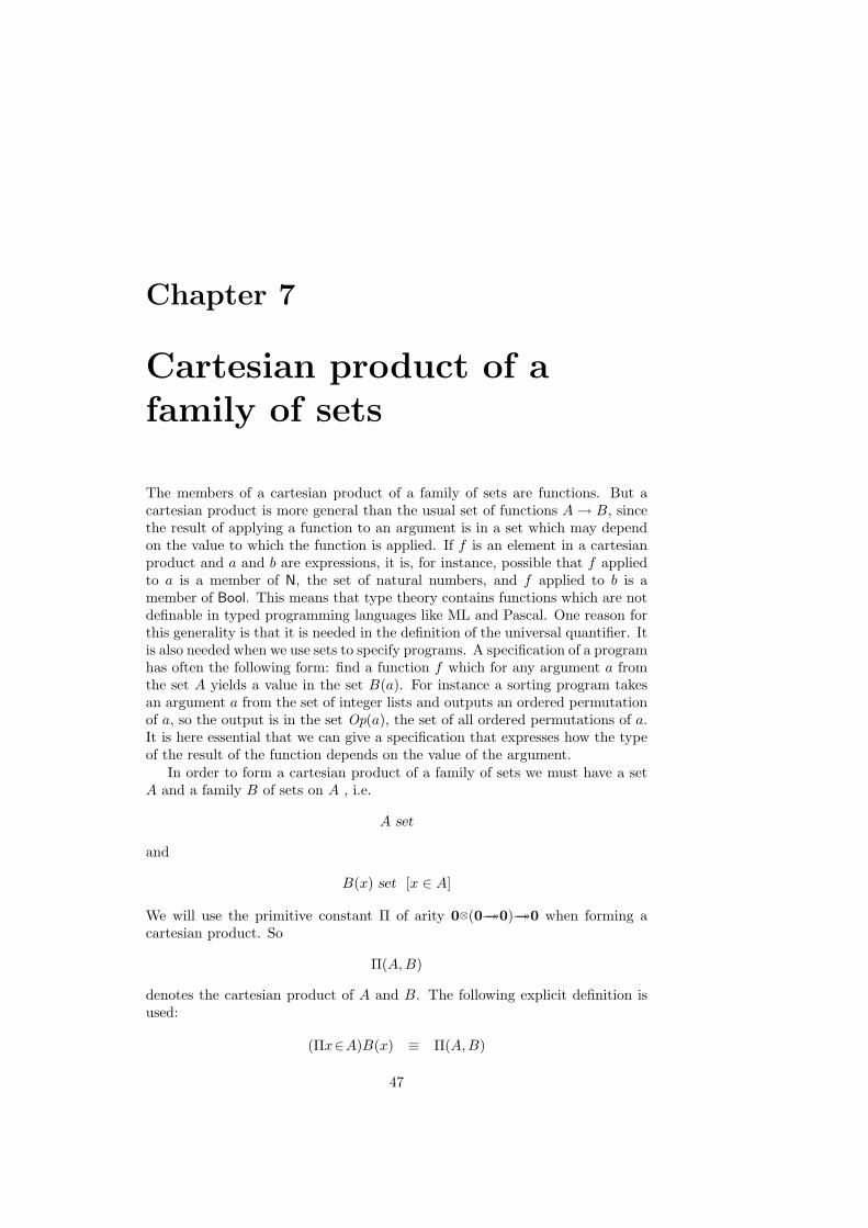
Chapter 7
Cartesian product of afamily of sets
The members of a cartesian product of a family of sets are functions. But acartesian product is more general than the usual set of functions A → B, sincethe result of applying a function to an argument is in a set which may dependon the value to which the function is applied. If f is an element in a cartesianproduct and a and b are expressions, it is, for instance, possible that f appliedto a is a member of N, the set of natural numbers, and f applied to b is amember of Bool. This means that type theory contains functions which are notdefinable in typed programming languages like ML and Pascal. One reason forthis generality is that it is needed in the definition of the universal quantifier. Itis also needed when we use sets to specify programs. A specification of a programhas often the following form: find a function f which for any argument a fromthe set A yields a value in the set B(a). For instance a sorting program takesan argument a from the set of integer lists and outputs an ordered permutationof a, so the output is in the set Op(a), the set of all ordered permutations of a.It is here essential that we can give a specification that expresses how the typeof the result of the function depends on the value of the argument.
In order to form a cartesian product of a family of sets we must have a setA and a family B of sets on A , i.e.
A set
and
B(x) set [x ∈ A]
We will use the primitive constant Π of arity 0⊗(0→→0)→→0 when forming acartesian product. So
Π(A,B)
denotes the cartesian product of A and B. The following explicit definition isused:
(Πx∈A)B(x) ≡ Π(A,B)
47

48 CHAPTER 7. CARTESIAN PRODUCT OF A FAMILY OF SETS
We have to define the canonical elements in Π(A,B) and define what it meansfor two canonical elements to be equal. The elements in Π(A,B) are functionsand we will use the lambda notation for expressing them. So we introduce theprimitive constant λ of arity (0→→0)→→0. The basic notion of function is anexpression formed by abstraction. Therefore the canonical elements in Π(A,B)will be formed by applying the λ on an abstraction b such that b(x) is an elementof B(x) when x ∈ A:
λ(b) is a canonical element in Π(A,B) if b(x) ∈ B(x) [x ∈ A].
The equality between two canonical elements λ(b1) and λ(b2) of Π(A,B) isderived from the equality on the family B(x) on A :
λ(b1) and λ(b2) are equal canonical elements in Π(A,B) providedthat b1(x) = b2(x) ∈ B(x) [x ∈ A].
The primitive non-canonical constant for the Π-set is apply of arity 0⊗0→→0.It is the constant used for applying an element in Π(A,B) to an element in A.Hence, it has the following computation rule:
1. apply(f, a) is evaluated by first evaluating f .
2. If f has value λ(b) then the value of apply(f, a) is the value of b(a).
We will later, in section 7.2, give an alternative non-canonical constant forthe Π-set.
One of the main reasons for introducing the Π-set is that it is needed wheninterpreting the universal quantifier, which has the following Heyting interpre-tation:
(∀x ∈ A)B(x) is true if we can construct a function which whenapplied to an element a in the set A, yields a proof of B(a).
If we identify the proposition B(x) with the family of sets B(x) [x ∈ A], and ifwe let the proofs of B(x) be represented by the elements in the set B(x) [x ∈ A],then the elements in the set Π(A,B) are exactly the functions mentioned in theHeyting interpretation. The elements in Π(A,B) therefore represent the proofsof (∀x∈A)B(x). So we see, that in order to cope with the universal quantifier,it is necessary to have this kind of generalized function set.
Other examples of sets (propositions) that are defined as special cases of thecartesian product are:
1. the restricted set of functions A → B, where the set B does not dependon the argument x ∈ A
2. the implication A⊃B.
3. the record type former in Pascal is a set (Πx ∈ {i1, . . . , in})B(x), themembers of which are tuples. The component of the tuple with the namej is in the set B(j). In Pascal the application apply(f, j) is written f.j.
The last example shows that a cartesian product of a family of sets is ageneralization of a cartesian product of a finite number of sets.

7.1. THE FORMAL RULES AND THEIR JUSTIFICATION 49
It is important to distinguish between the two different notions of functionwe have used. The first is the fundamental syntactical notion of function as anexpression with holes in it, i.e. an expression which is not saturated. The secondis the notion of function as an element in the cartesian product. When there isa risk of confusion between these two notions, we will use the word abstractionfor the syntactic notion and function element for the second. The syntacticalnotion of function is more basic; we use it already when we write down the setsΠ(A,B) and A → C, in these expressions B, Π and → are abstractions.
Examples of canonical elements in different Π-sets are:
λ((x)x) ∈ Π(Bool, (x)Bool)λ(succ) ∈ Π(N, (x)N)
λ((x)λ((y)x + y)) ∈ Π(N, (x)Π(N, (y)N))
where N is the set of natural numbers and succ and + the usual arithmeticaloperations, to be introduced in chapter 9. These expressions can also be written:
λx.x ∈ (Πx∈Bool)Boolλx.succ(x) ∈ (Πx∈N)N
λx.λy.x + y ∈ (Πx∈N)(Πx∈N)N
An example of a non-canonical expression is:
apply(λx.x, false) ∈ Bool
The computation rule for apply justifies the equality
apply(λ(b), a) = b(a) ∈ B(a)
For example,
apply(λx.x, false) = false ∈ Bool
and
apply(λx.if x then 0 else false), true) = if true then 0 else false ∈ N
which can be further evaluated to 0.
7.1 The formal rules and their justification
As defined previously, the canonical elements in Π(A,B) are of the form λ(b),where b(x) ∈ B(x) when x ∈ A. We also defined two canonical elements λ(b1)and λ(b2) in Π(A,B) to be equal if b1(x) = b2(x) ∈ B(x) when x ∈ A. Inorder to see that Π(A,B) is a set it only remains to verify that the equality onΠ(A,B) is extensional. But this is obvious since the free variables in λ(b1) andλ(b2) are also free in b1(x) and b2(x) and the equality on the family B(x) overA is required to be extensional.
Therefore, Π(A,B) is a set if A is a set and if B(x) is a set under theassumption that x ∈ A. Hence, the formation rule is:
Π – formation
A set B(x) set [x ∈ A]Π(A,B) set

50 CHAPTER 7. CARTESIAN PRODUCT OF A FAMILY OF SETS
Since the canonical elements in the set Π(A,B) are of the form λ(b) whereb(x) ∈ B(x) under the assumption that x ∈ A, we get
Π – introduction
b(x) ∈ B(x) [x ∈ A]λ(b) ∈ Π(A,B)
As mentioned earlier, the primitive non-canonical constant for the cartesianproduct is
apply
of arity 0⊗0→→0. We also introduce an infix form of apply by the definition
x · y ≡ apply(x, y)
The rule associated with apply is:Π – elimination 1
f ∈ Π(A,B) a ∈ A
apply(f, a) ∈ B(a)
We have to convince ourselves, from the way apply(f, a) is computed and thesemantics of the judgement forms, that this rule is correct. That f ∈ Π(A,B)means that
f has a value of the form λ(b) (1)
whereb(x) ∈ B(x) [x ∈ A] (2)
since it must have a canonical value in the set Π(A,B) and all canonical valuesof Π(A,B) have this form. By the definition of how apply(f, a) is computed and(1), we get that
apply(f, a) is computed by computing b(a). (3)
Since a ∈ A, we get from (2) that
b(a) ∈ B(a) (4)
(3) and (4) finally give usapply(f, a) ∈ B(a)
and thereby the elimination rule is justified.The way apply(f, a) is computed gives the rule:
Π – equality 1
b(x) ∈ B(x) [x ∈ A] a ∈ A
apply(λ(b), a) = b(a) ∈ B(a)
since b(x) ∈ B(x) [x ∈ A] and a ∈ A give that b(a) ∈ B(a).

7.2. AN ALTERNATIVE PRIMITIVE NON-CANONICAL FORM 51
7.2 An alternative primitive non-canonical form
As an example of how the semantics can justify the introduction of a differentnon-canonical form, we will introduce an alternative to the selector apply in theΠ-set.
For most sets, the non-canonical forms and their computation rules are basedon the principle of structural induction. This principle says, that to prove thata property B(a) holds for an arbitrary element a in the set A, prove that theproperty holds for each of the canonical elements in A. Similarly, to constructa program for an arbitrary element a in the set A, construct a program for eachof the canonical forms of A. The computation rule for the non-canonical formin the Π-set does not follow this principle. It is chosen because the rule is well-known from the λ-calculus (β-reduction). The alternative non-canonical form isbased on the principle of structural induction. We define the new non-canonicalform as follows:
Introduce the constant funsplit of arity (0⊗((0→→0)→→0))→→0 and let theexpression funsplit(f, d) be computed by the following rule:
1. Compute f .
2. If the value of f is λ(b), then the value of funsplit(f, d) is the value ofd(b).
The expression f is to be an arbitrary element in the set Π(A,B) and d(y) isa program in the set C(λ(y)) under the assumption that y(x) ∈ B(x) [x ∈A]. Notice that this is a higher order assumption, an assumption in which anassumption is made. The variable y is of arity 0→→0, i.e. it is a function variable,i.e. a variable standing for an abstraction. Note that a function variable issomething quite different from an element variable ranging over a Π set.
The alternative elimination rule becomes:Π – elimination 2
f ∈ Π(A,B)C(v) set [v ∈ Π(A,B)]d(y) ∈ C(λ(y)) [y(x) ∈ B(x) [x ∈ A]]funsplit(f, d) ∈ C(f)
We can justify Π-elimination 2 in the following way: If f ∈ Π(A,B) it followsfrom the meaning of this judgement form that f must have a canonical elementas value. The canonical elements in the Π set are of the form λ(b), so f has avalue of the form λ(b) and
f = λ(b) ∈ Π(A,B) (1)
whereb(x) ∈ B(x) [x ∈ A] (2)
Since we know that d(y) ∈ C(λ(y)) whenever y(x) ∈ B(x) [x ∈ A] and b(x) ∈B(x) [x ∈ A], we get
d(b) ∈ C(λ(b)) (3)
From the computation rule for funsplit and from (1) we can conclude thatfunsplit(f, d) is computed by computing d(b) and from (3) it follows that
funsplit(f, d) ∈ C(λ(b)) (4)

52 CHAPTER 7. CARTESIAN PRODUCT OF A FAMILY OF SETS
From the premise that C(v) is a set under the assumption that v ∈ Π(A,B) andfrom (1) it follows that
C(f) = C(λ(b)) (5)
and now from (4) and (5) and the meaning of the judgement form A = B, itimmediately follows that
funsplit(f, b) ∈ C(f)
Hence, the first elimination rule is justified.The computation rule for funsplit(λ(b), b) gives the equality rule:
Π – equality 2
b(x) ∈ B(x) [x ∈ A]C(v) set [v ∈ Π(A,B)]d(y) ∈ C(λ(y)) [y(w) ∈ B(w) [w ∈ A]]funsplit(λ(b), d) = d(b) ∈ C(λ(b))
since b(x) ∈ B(x) [x ∈ A] and d(y) ∈ C(λ(y)) [y(w) ∈ B(w) [w ∈ A]] gived(b) ∈ C(λ(b)).
Now we can reintroduce the constant apply of arity 0⊗0→→0 by making anexplicit definition
apply(f, a) ≡ funsplit(f, (x)(x(a)))
If we have defined apply in this way, the expression apply(f, a) will be com-puted in the following way. The program apply(f, a) is definitionally equal tofunsplit(f, (x)(x(a))) which is computed by first computing the value of f . If thevalue is λ(b) then continue to compute the value of the program ((x)(x(a)))(b),a program which is definitionally equal to b(a).
We can also prove a counterpart to the first Π-elimination rule:
Theorem If a ∈ A and f ∈ Π(A,B), then apply(f, a) ∈ B(a).
Proof: Assume that a ∈ A and f ∈ Π(A,B). For some expression b, f mustbe equal to λ(b) where
b(x) ∈ B(x) [x ∈ A] (1)
Using the definition of apply, we get that apply(f, a) is computed by computingfunsplit(λ(b), (x)x(a)). The computation rule for funsplit gives that apply(f, a)is equal to b(a). From (1) we get
b(a) ∈ B(a)
Hence,
apply(f, a) ∈ B(a)
2
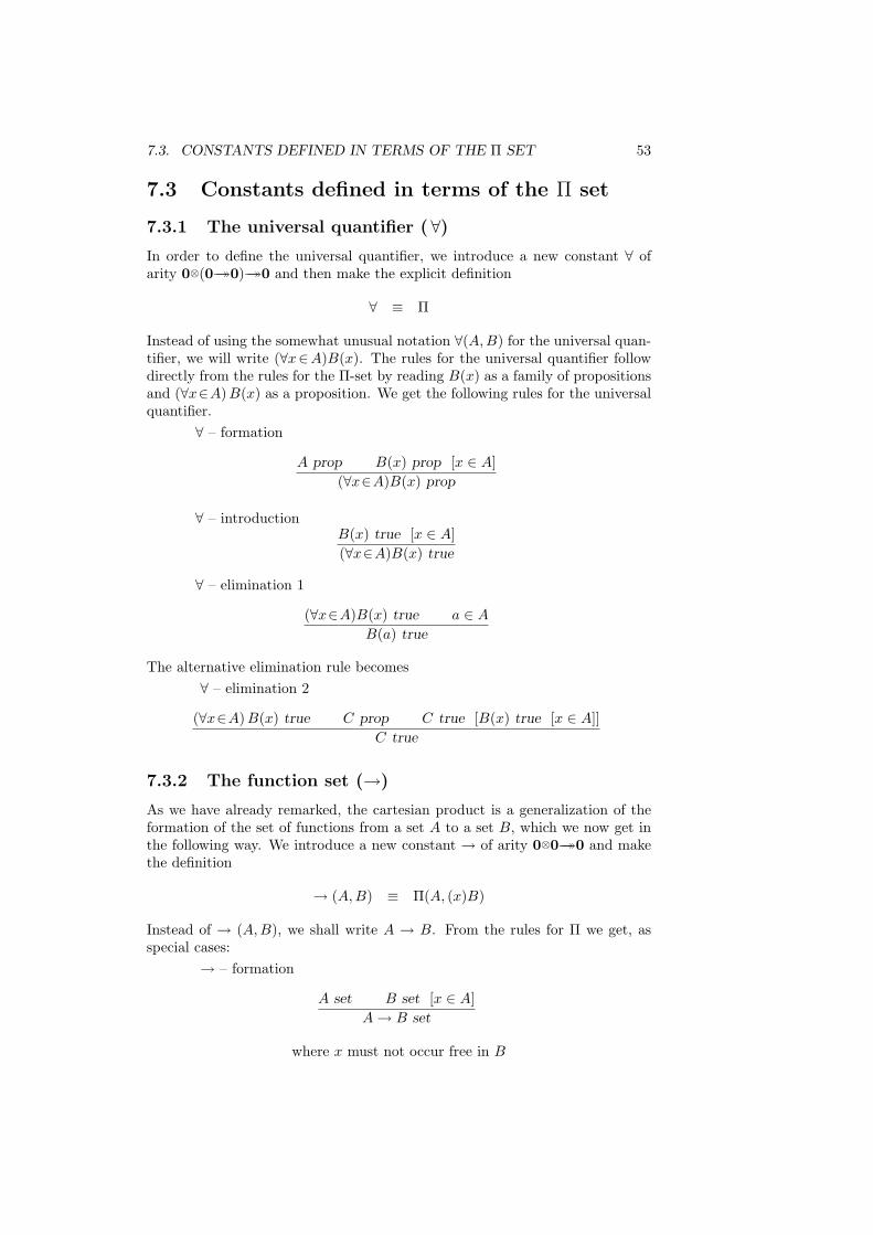
7.3. CONSTANTS DEFINED IN TERMS OF THE Π SET 53
7.3 Constants defined in terms of the Π set
7.3.1 The universal quantifier (∀)In order to define the universal quantifier, we introduce a new constant ∀ ofarity 0⊗(0→→0)→→0 and then make the explicit definition
∀ ≡ Π
Instead of using the somewhat unusual notation ∀(A,B) for the universal quan-tifier, we will write (∀x∈A)B(x). The rules for the universal quantifier followdirectly from the rules for the Π-set by reading B(x) as a family of propositionsand (∀x∈A) B(x) as a proposition. We get the following rules for the universalquantifier.
∀ – formation
A prop B(x) prop [x ∈ A](∀x∈A)B(x) prop
∀ – introductionB(x) true [x ∈ A](∀x∈A)B(x) true
∀ – elimination 1
(∀x∈A)B(x) true a ∈ A
B(a) true
The alternative elimination rule becomes∀ – elimination 2
(∀x∈A) B(x) true C prop C true [B(x) true [x ∈ A]]C true
7.3.2 The function set (→)
As we have already remarked, the cartesian product is a generalization of theformation of the set of functions from a set A to a set B, which we now get inthe following way. We introduce a new constant → of arity 0⊗0→→0 and makethe definition
→ (A,B) ≡ Π(A, (x)B)
Instead of → (A,B), we shall write A → B. From the rules for Π we get, asspecial cases:
→ – formation
A set B set [x ∈ A]A → B set
where x must not occur free in B

54 CHAPTER 7. CARTESIAN PRODUCT OF A FAMILY OF SETS
→ – introductionb(x) ∈ B [x ∈ A]
λ(b) ∈ A → B
where x must not occur free in B
→ – eliminationf ∈ A → B a ∈ A
apply(f, a) ∈ B
→ – equality
b(x) ∈ B [x ∈ A] a ∈ A
apply(λ(b), a) = b(a) ∈ B
where x must not occur free in B or f
7.3.3 Implication (⊃ )
The Heyting interpretation of implication is
The implication A⊃B is true if we can construct a function whichwhen applied to a proof of A, yields a proof of B.
If we let the elements in the set A represent the proofs of the proposition Aand similarly for the set (proposition) B, then we can see that the elements(functions) of A → B are exactly the constructions we require in the Heytinginterpretation to prove A⊃B. So we get the implication A⊃B simply by in-troducing a new constant ⊃ of arity 0⊗0→→0 and making the explicit definition
⊃ ≡ →
The rules for implication immediately follow from the rules for →. By omittingthe proof elements in the rules for implication we get the natural deductionrules:
⊃ – formationA prop B prop [A true]
A⊃B prop
⊃ – introductionB true [A true]
A⊃B true
⊃ – eliminationA⊃B true A true
B true
The alternative elimination rule becomes:A⊃B true C prop C true [B true [A true]]
C true
Notice that the second premise of the formation rule is weaker than in thetraditional rule. To show that A⊃B is a proposition it is enough to show thatA is a proposition and that B is a proposition under the assumption that A istrue This rule has been suggested by Schroeder-Heister [96].

7.3. CONSTANTS DEFINED IN TERMS OF THE Π SET 55
Example. Changing the order of universal quantifiers
From a constructive proof in natural deduction, it is always possible to obtain,by filling in the omitted constructions, a proof in type theory. Consider, forinstance, the following proof in natural deduction:
Assume
(∀x∈N)(∀y∈Bool) Q(x, y)
∀-elimination used twice, gives
Q(x, y) [x ∈ N, y ∈ Bool]
By ∀-introduction (twice) we get
(∀y∈Bool)(∀x∈N) Q(x, y)
Finally by ⊃ -introduction
(∀x∈N)(∀y∈Bool) Q(x, y)⊃ (∀y∈Bool)(∀x∈N)Q(x, y)
With the proof elements present, this proof becomes:Assume
w ∈ (Πx∈N)(Πy∈Bool) Q(x, y)
By Π-elimination (twice) we get
apply2(w, x, y) ∈ Q(x, y) [x ∈ N, y ∈ Bool]
where
apply2(x, y, z) ≡ apply(apply(x, y), z)
and then by Π-introduction (twice)
λy.λx.apply2(w, x, y) ∈ (Πy∈Bool)(Πx∈N) Q(x, y)
Finally, by →-introduction
λw.λy.λx.apply2(w, x, y) ∈(Πx∈N)(Πy∈Bool)Q(x, y) → (Πy∈Bool)(Πx∈N)Q(x, y)
56 CHAPTER 7. CARTESIAN PRODUCT OF A FAMILY OF SETS

Chapter 8
Equality sets
We have seen how to use set-forming operations to build up complex propo-sitions from simpler ones, but so far we have only introduced the elementarypropositions T (the truth) and ⊥ (the absurdity). Since the judgemental equal-ity cannot be used when building propositions, it is necessary to have an ele-mentary proposition expressing that two elements are equal. Beside the equalitysets, it is the universe and general trees, which are introduced later, which makeit possible to have dependent sets.
We will introduce two different sets to express that a and b are equal elementsof a set A. The first one, which we denote by Id(A, a, b) and which we will callintensional equality, will have an elimination rule which expresses an inductionprinciple. The second one, which we denote by Eq(A, a, b), will have a strongelimination rule of a different form than the elimination rules for the other sets.With this set, judgemental equality will no longer be decidable and we willtherefore avoid this equality when possible. It is only in the chapters on well-orderings and general trees we must use it. In the chapter on cartesian productof two sets, we will show that extensionally equal functions are equal in thesense of Eq. Hence, we will call these kind of equalities extensional equalities.
8.1 Intensional equality
The set Id(A, a, b), where Id is a primitive constant of arity 0⊗0⊗0→→0, willrepresent the judgement a = b ∈ A as a set.
Id – formation
A set a ∈ A b ∈ A
Id(A, a, b) set
The set Id(A, a, a) will have the member id(a) where a ∈ A and id is a primitiveconstant of arity 0→→0. So we have
Id – introductiona ∈ A
id(a) ∈ Id(A, a, a)
By using Substitution in sets on a = b ∈ A and Id(A, a, x) set [x ∈ A] we obtainId(A, a, a) = Id(A, a, b). So, by Id –introduction 1 and Set equality we get thederived rule
57

58 CHAPTER 8. EQUALITY SETS
Id – introduction’a = b ∈ A
id(a) ∈ Id(A, a, b)
The primitive non-canonical constant of the equality set is idpeel of arity
(0⊗(0→→0))→→0
The expression idpeel(c, d) is computed as follows:
1. idpeel(c, d) is evaluated by first evaluating c.
2. If c has value id(a) then the value of idpeel(c, d) is the value of d(a).
The way a canonical element is introduced in an equality set and the computa-tion rule for idpeel justifies the elimination rule:
Id – elimination
a ∈ Ab ∈ Ac ∈ Id(A, a, b)C(x, y, z) set [x ∈ A, y ∈ A, z ∈ Id(A, x, y)]d(x) ∈ C(x, x, id(x)) [x ∈ A]idpeel(c, d) ∈ C(a, b, c)
As for the other sets, the elimination rule expresses a principle of structuralinduction on an equality set, but the importance of the elimination rule in thiscase is more in that it is a substitution rule for elements which are equal in thesense of an equality set.
The way idpeel(c, d) is computed gives the rule:Id – equality
a ∈ AC(x, y, z) set [x ∈ A, y ∈ A, z ∈ Id(A, x, y)]d(x) ∈ C(x, x, id(x)) [x ∈ A]idpeel(id(a), d) = d(a) ∈ C(a, a, id(a))
Instead of Id(A, a, b) we will often write a =A b.
Example. Symmetry and transitivity of equality
Let A be a set and a and b elements of A. Assume that
d ∈ Id(A, a, b) (8.1)
In order to prove symmetry, we must construct an element in Id(A, b, a). Byputting C ≡ (x, y, z)Id(A, y, x) in Id-elimination we get, by Id-introduction,
idpeel(d, id) ∈ Id(A, b, a)
so we have proved symmetry. Hence, we have the following derived rule:Symmetry of propositional equality
d ∈ [a =A b]symm(d) ∈ [b =A a]

8.1. INTENSIONAL EQUALITY 59
wheresymm(d) ≡ idpeel(d, id)
To prove transitivity, we assume
e ∈ Id(A, b, c) (8.2)
where c is an element in A. We then have to construct an element in Id(A, a, c).Using Id-elimination with C ≡ (x, y, z)(Id(A, y, c) → Id(A, x, c)) we get fromd ∈ Id(A, a, b), by Π-introduction,
idpeel(d, (x)λy.y) ∈ Id(A, b, c) → Id(A, a, c) (8.3)
(8.2), (8.3) and Π-elimination give
apply(idpeel(d, (x)λy.y), e) ∈ Id(A, a, c)
and, hence, we have transitivity. So we have the following derived rule:Transitivity of propositional equality
d ∈ [a =A b] e ∈ [b =A c]trans(d, e) ∈ [a =A c]
wheretrans(d, e) ≡ apply(idpeel(d, (x)λy.y), e)
Example. Substitution with equal elements
Assume that we have a set A and elements a and b of A. Assume also thatc ∈ Id(A, a, b), P (x) set [x ∈ A] and p ∈ P (a). By Π-introduction we get
λx.x ∈ P (x) → P (x)
Putting C ≡ (x, y, z)(P (x) → P (y)) in Id-elimination we then get
idpeel(c, (x)λx.x) ∈ P (a) → P (b)
from which we obtain, by Π-elimination,
apply(idpeel(c, (x)λx.x), p) ∈ P (b)
So we have the derived rule
P (x) set [x ∈ A] a ∈ A b ∈ A c ∈ Id(A, a, b) p ∈ P (a)subst(c, p) ∈ P (b)
wheresubst(c, p) ≡ apply(idpeel(c, (x)λx.x), p)
If we suppress the proof-objects we get the rule
P (x) set [x ∈ A] a ∈ A b ∈ A Id(A, a, b) true P (a) true
P (b) true
which corresponds to the usual substitution rule in predicate logic with equality.

60 CHAPTER 8. EQUALITY SETS
Example. An equality involving the conditional expression
In this example we will prove, that for any set A
Id(A, if b then c else c, c) [b ∈ Bool, c ∈ A]
is inhabited. We start by assuming that c ∈ A and b ∈ Bool. and will show thatthere is an element in Id(A, if b then c else c, c) by case analysis on b.
1. b = false: The Bool – equality rule gives
if false then c else c = c ∈ A
which, using Id – introduction, gives
id(c) ∈ Id(A, if false then c else c, c)
2. b = true: In the same way as above, we first get
if true then c else c = c ∈ A
by one of the Bool – equality rules, and then
id(c) ∈ Id(A, if true then c else c, c)
by Id – introduction.
Applying the Bool – elimination rule on the two cases, we finally get
if b then id(c) else id(c) ∈ Id(A, if b then c else c, c)
8.2 Extensional equality
We will now give an alternative formulation of equality sets which will have astrong elimination rule of a different form than all the other sets.
In the semantics we have given, following [69, 70], the judgemental equalityis more general than convertibility; we have only required that it should be anequivalence relation which is extensional with respect to substitution. The rulesfor the equality sets given in [69, 70] are different from those we are using. Theformation rule is
Eq – formation
A set a ∈ A b ∈ A
Eq(A, a, b) set
where Eq is a primitive constant of arity 0⊗0⊗0→→0.There is at most one canonical element in an Eq-set:
Eq – introductiona = b ∈ A
eq ∈ Eq(A, a, b)
which differs from the introduction rule for Id-sets in that eq is of arity 0 and,hence, a canonical element of Eq(A, a, b) does not depend on an element in A.The crucial difference, however, is the elimination rule:

8.2. EXTENSIONAL EQUALITY 61
Strong Eq – elimination
c ∈ Eq(A, a, b)a = b ∈ A
Unlike the elimination rules for the other sets, this elimination rule is not astructural induction principle.
We also need an elimination rule by which we can deduce that all elementsin an Eq are equal to eq:
Eq – elimination 2
c ∈ Eq(A, a, b)c = eq ∈ Eq(A, a, b)
Using the two elimination rules for Eq, we can derive an induction rule forEq, corresponding to Id-elimination,
a ∈ Ab ∈ Ac ∈ Eq(A, a, b)C(x, y, z) set [x ∈ A, y ∈ A, z ∈ Eq(A, x, y)]d(x) ∈ C(x, x, eq) [x ∈ A]d(a) ∈ C(a, b, c)
To prove this rule, we assume the premises of the rule. By strong Eq-eliminationand c ∈ Eq(A, a, b), we get
a = b ∈ A (8.1)
From a ∈ A and d(x) ∈ C(x, x, eq) [x ∈ A] we obtain, by substitution,
d(a) ∈ C(a, a, eq) (8.2)
(1), Eq-elimination 2, (2) and substitution, finally give
d(a) ∈ C(a, b, c) (8.3)
If we do not have sets formed by Eq in our formal theory it is possible toshow, by metamathematical reasoning, that if a = b ∈ A is derivable then aconverts to b. That a converts to b is then understood in the usual way ofcombinatory logic with our computational rules for the noncanonical constantsas reduction rules; in particular, it is not necessary to have lazy evaluation.The proof is by induction on the length of the derivation of a = b ∈ A. It isalso possible to show that if c ∈ Id(A, a, b) is derivable and does not depend onany assumptions, then a converts to b; this is the reason why we call equalitiesformed by Id intensional. This result can be proved by normalization; such aproof is complicated but can be done, using standard techniques.
If we express propositional equalities by Eq it is no longer possible to under-stand judgemental equality as convertibility, because it is then possible to provea judgemental equality by reasoning using propositions. So we may e.g. use in-duction when proving a judgement of the form a(x) = b(x) ∈ A [x ∈ N] by firstproving Eq(A, a(x), b(x)) [x ∈ N] and then applying the strong Eq-eliminationrule.

62 CHAPTER 8. EQUALITY SETS
8.3 η-equality for elements in a Π set
We have not formulated any judgemental rule corresponding to η-conversion,that is, we have no rule by which we can conclude
λ((x)apply(f, x)) = f ∈ Π(A,B) [f ∈ Π(A,B)]
Although we do not have this judgemental equality we can prove, by usingΠ-elimination 3, that the corresponding Id judgement holds:
Id(Π(A,B), λ((x)apply(f, x)), f) true [f ∈ Π(A,B)] (1)
(1) can be derived in the following way. By Π-equality we obtain
λ((x)apply(λ(y), x)) = λ(y) ∈ Π(A,B) [y(x) ∈ B(x) [x ∈ A]]
from which we get, by Id-introduction,
id(λ(y)) ∈ Id(Π(A,B), λ((x)apply(λ(y), x)), λ(y)) [y(x) ∈ B(x) [x ∈ A]] (2)
PuttingD(λ(y)) ≡ Id(Π(A,B), λ((x)apply(λ(y), x)), λ(y))
in Π-elimination 3, we obtain from (2)
funsplit(f, (y)id(λ(y))) ∈ Id(Π(A,B), λ((x)apply(f, x)), f) [f ∈ Π(A,B)]
which shows that the judgement (1) holds.A similar proof for Eq instead of Id gives a term t such that
t ∈ Eq(Π(A,B), λ((x)apply(f, x)), f) [f ∈ Π(A,B)]
By strong Eq-elimination, we then obtain
λ((x)apply(f, x)) = f ∈ [f ∈ Π(A,B)]
So in the theory with Eq-sets, we have η-conversion on the judgemental level.

Chapter 9
Natural numbers
The constant N of arity 0 denotes the set of natural numbers. The rule forforming this set is simply
N – formation
N set
The canonical constants 0 and succ of arities 0 and 0→→0 respectively, are usedfor expressing the canonical elements in N. The object 0 is a canonical elementin N and if a is an element in N then succ(a) is a canonical element in N. Thisis reflected in the following introduction rules:
N – introduction 1
0 ∈ N
N – introduction 2a ∈ N
succ(a) ∈ N
We will often use the numerals 1, 2, . . . to denote canonical elements in N.If a and b are equal elements in N then succ(a) and succ(b) are equal canonical
elements in N.The basic way of proving that a proposition holds for all natural numbers is
by mathematical induction: From P (0) and that P (x) implies P (succ(x)) youmay conclude that P (n) holds for all natural numbers n. In order to be able toprove properties by induction on natural numbers in type theory, we introducethe selector natrec of arity 0⊗0⊗(0⊗0→→0)→→0. From a computational point ofview, natrec makes it possible to make definitions by primitive recursion. Theexpression natrec(a, d, e) is computed as follows.
1. Evaluate a to canonical form.
2a. If the result of evaluating a is 0 then the value of the expression is thevalue of d.
2b. If the result of evaluating a is succ(b) then the value of the expressionis the value of e(b, natrec(b, d, e)).
63

64 CHAPTER 9. NATURAL NUMBERS
So, defining a function f by the primitive recursion{f(0) = df(n⊕1) = e(n, f(n))
is in type theory expressed by the definition
f ≡ (n)natrec(n, d, e)
For example, using natrec, we can define the constants ⊕ and ∗ of arity 0⊗0→→0by the explicit definitions
⊕(x, y) ≡ natrec(x, y, (u, v) succ(v))∗(x, y) ≡ natrec(x, 0, (u, v)⊕(y, v))
expressing addition and multiplication, respectively. We will use the infix formatand the ordinary precedence rules for ⊕ and ∗. These definitions correspondexactly to the usual definitions of addition and multiplication by primitive re-cursion.
The elimination rule for the natural numbers is:N – elimination
a ∈ Nd ∈ C(0)C(v) set [v ∈ N]e(x, y) ∈ C(succ(x)) [x ∈ N, y ∈ C(x)]natrec(a, d, e) ∈ C(a)
In order to justify N-elimination we assume the premises a ∈ N, d ∈ C(0) ande(x, y) ∈ C(succ(x)) [x ∈ N, y ∈ C(x)]. We want to convince ourselves that theconclusion is correct, i.e. that the value of natrec(a, d, e) is a canonical elementin C(a)
1. If the value of a is 0 then the value of natrec(a, d, e) is the value of dwhich by the second premise is a canonical element in C(0). From theextensionality of the family C it follows that C(a) = C(0) and, hence,that the value of natrec(a, d, e) is a canonical element in C(a).
2. If the value of a is succ(b), where b ∈ N, then the value of natrec(a, d, e) isthe value of
e(b, natrec(b, d, e)) (1)
It now remains to show that natrec(b, d, e) ∈ C(b). Then it follows fromthe meaning of the last premise that the value of (1) is a canonical elementin C(succ(b)) which by the extensionality of C is also a canonical elementin C(a). To show that natrec(b, d, e) ∈ C(b) we compute the value ofnatrec(b, d, e) by first computing b. The value of b is either 0 or succ(c),where c ∈ N.
(a) If the value of b is 0 then by a similar reasoning as in (1) we concludethat the value of natrec(b, d, e) is a canonical element in C(b).

65
(b) Otherwise, if the value of b is succ(c), where c ∈ N, then we proceedas in (2) to show that the value of natrec(b, d, e) is a canonical elementin C(b). This method will terminate since all natural numbers areobtained by applying the successor function to 0 a finite number oftimes.
If some of the constructions in the elimination rule are omitted, Peano’s fifthaxiom is obtained:
a ∈ N C(v) prop [v ∈ N] C(0) true C(succ(x)) true [C(x) true]C(a) true
Notice that the justification of the induction rule comes from N-eliminationwhich was justified by using mathematical induction on the semantical level. Ofcourse, neither N-elimination nor Peano’s fifth axiom can be justified without theknowledge that N is well-founded, which is something which we must understandfrom the inductive definition of the canonical elements in N, that is, from theintroduction rules for N.
Finally we have the equality rules, which are justified from the computationrule for natrec.
N – equality 1
C(v) set [v ∈ N]d ∈ C(0)e(x, y) ∈ C(succ(x)) [x ∈ N, y ∈ C(x)]natrec(0, d, e) = d ∈ C(0)
N – equality 2
C(v) set [v ∈ N]a ∈ Nd ∈ C(0)e(x, y) ∈ C(succ(x)) [x ∈ N, y ∈ C(x)]natrec(succ(a), d, e) = e(a, natrec(a, d, e)) ∈ C(succ(a))
The proposition in type theory corresponding to Peano’s fourth axiom needsthe Universe set to be proved, so we have to postpone this until later.
Example. The typing of the ⊕ -operator
The constant ⊕ was defined by
⊕(x, y) ≡ natrec(x, y, (u, v) succ(v))
We will now formally show that
⊕(x, y) ∈ N [x ∈ N, y ∈ N]
By the rule of assumption we get
x ∈ N [x ∈ N] (9.1)y ∈ N [y ∈ N] (9.2)

66 CHAPTER 9. NATURAL NUMBERS
Assumption and N-introduction 2 give
succ(v) ∈ N [v ∈ N] (9.3)
By applying N-elimination on (9.1), (9.2) and (9.3) we get
natrec(x, y, (u, v) succ(v)) ∈ N [x ∈ N, y ∈ N]
that is, by definition,⊕(x, y) ∈ N [x ∈ N, y ∈ N]
Example. Peano’s third axiom
Peano’s third axiom is that if the successor of two natural numbers are equalthen the natural numbers are equal. We can formulate this in type theory as aderived rule:
m ∈ N n ∈ N succ(m) = succ(n) ∈ N
m = n ∈ N
In the derivation of this rule we will use the predecessor function pred, which isdefined by
pred ≡ (x)natrec(x, 0, (u, v)u)
Since 0 ∈ N and u ∈ N [u ∈ N], the definition of pred and N-elimination give
pred(x) ∈ N [x ∈ N] (9.1)
Let m ∈ N, n ∈ N andsucc(m) = succ(n) ∈ N (9.2)
By (9.1), (9.2) and Substitution in equal elements, we get
pred(succ(m)) = pred(succ(n)) ∈ N (9.3)
The definition of pred and N-equality 2 give
pred(succ(m)) = m ∈ N (9.4)pred(succ(n)) = n ∈ N (9.5)
Using symmetry and transitivity of judgemental equality on (9.3) – (9.5), wefinally obtain
m = n ∈ N
and, hence we have Peano’s third axiom as a derived rule.Instead of formulating Peano’s third axiom as a derived rule, we could ex-
press it as a proposition, using an equality set:
(∀x∈N)(∀y∈N)(Id(N, succ(x), succ(y))⊃ Id(N, x, y))
This proposition can be proved in a similar way as the derived rule, using therules for Id instead of the rules for judgemental equality. Note that these two for-mulations of Peano’s third axiom are inherently different: the first formulationis about judgements but the second is a proposition.

Chapter 10
Lists
In order to form the set of lists of elements in a set A, we introduce three newconstants: List of arity 0→→0, nil of arity 0 and cons of arity 0⊗0→→0. If A is aset, then the canonical elements in List(A) are nil and cons(a, l) where a is anelement in A and l is an element in List(A). If a = a′ ∈ A and l = l′ ∈ List(A)then cons(a, l) and cons(a′, l′) are equal canonical elements in List(a).
We have the following rule for forming list sets.List – formation
A set
List(A) set
In order to be able to use infix notation when constructing lists, we make thedefinition
a.l ≡ cons(a, l)
The introduction rules are:List – introduction
nil ∈ List(A)a ∈ A l ∈ List(A)
a.l ∈ List(A)
The primitive non-canonical constant listrec of arity 0⊗0⊗(0⊗0⊗0→→0)→→0 isintroduced in order to express recursion on lists. The expression listrec(l, c, e) iscomputed as follows:
1. First compute l.
2a. If the value of l is nil, then the value of listrec(l, c, e) is the value of c.
2b. If the value of l is a.l1 then the value of listrec(l, c, e) is the value ofe(a, l1, listrec(l1, c, e)).
The following rules are justified in the same way as the corresponding rules fornatural numbers:
67

68 CHAPTER 10. LISTS
List – elimination
l ∈ List(A)C(v) set [v ∈ List(A)]c ∈ C(nil)e(x, y, z) ∈ C(x.y) [x ∈ A, y ∈ List(A), z ∈ C(y)]
listrec(l, c, e) ∈ C(l)
List – equality 1
C(v) set [v ∈ List(A)]c ∈ C(nil)e(x, y, z) ∈ C(x.y) [x ∈ A, y ∈ List(A), z ∈ C(y)]
listrec(nil, c, e) = c ∈ C(nil)
List – equality 2
a ∈ Al ∈ List(A)C(v) set [v ∈ List(A)]c ∈ C(nil)e(x, y, z) ∈ C(x.y)) [x ∈ A, y ∈ List(A), z ∈ C(y)]
listrec(a.l, c, e) = e(a, l, listrec(l, c, e)) ∈ C(a.l)
Example. Associativity of append
The function append concatenates two lists and is defined by
append(l1, l2) ≡ listrec(l1, l2, (x, y, z) x.z))
We will use the binary infix operator @ for append,
l1@l2 ≡ append(l1, l2)
From the List-elimination rule, it follows directly that
l1@l2 ≡ listrec(l1, l2, (x, y, z) x.z) ∈ List(A) [l1 ∈ List(A), l2 ∈ List(A)]
By applying List-equality to the definition of l1@l2 we get the following equalities{nil@l2 = l2 ∈ List(A)a.l1@l2 = a.(l1@l2) ∈ List(A)
which are the usual defining equations for append.As a simple example, we are going to show how to formally prove that @ is
associative, i.e. if p, q, r ∈ List(A) then
p@(q@r) =List(A) (p@q)@r
is a true proposition. We will write L instead of List(A). We first give theinformal proof and then translate it to a proof in type theory.
We sometimes use the following notation, introduced by Dijkstra, for infor-mal proofs:

69
t1= { informal argument why t1 = t2 }
t2= { informal argument why t2 = t3 }
t3
This is sometimes generalized from equality to another transitive operator.The proof proceeds by induction on the list p. For the base case, we have to
show that nil@(q@r) =L (nil@q)@r, which is done by simplifying the two sides ofthe equation:
nil@(q@r)= { definition of @ }
q@r
(nil@q)@r= { definition of @, substitution }
q@r
The induction step starts in a similar way and ends in using the inductionhypothesis. We are going to show that (x.y)@(q@r) =L ((x.y)@q)@r from theassumption that y@(q@r) =L (y@q)@r. First, the left hand side:
(x.y)@(q@r)= { definition of @ }
x.(y@(q@r))
Then the right hand side:
((x.y)@q)@r= { definition of @, substitution }
(x.(y@q))@r= { definition of @ }
x.((y@q)@r)=L { induction assumption, substitution }
x.(y@(q@r))
The proof is by induction on the list p, so in type theory we use List-elimination. We have to prove the three premises
1. p ∈ L, which we already have assumed.
2. Find an element in [nil@(q@r) =L (nil@q)@r].
3. Under the assumptions that x ∈ A, y ∈ L and z ∈ [y@(q@r) =L (y@q)@r]find an element in [(x.y)@(q@r) =L ((x.y)@q)@r].

70 CHAPTER 10. LISTS
The following is a formal proof of the two parts in the base step. First wehave the simplification of the left hand side:
q ∈ L r ∈ L
q@r ∈ L
x ∈ A z ∈ L
x.z ∈ LList−intro
listrec(nil, (q@r), (x, y, z)x.z)︸ ︷︷ ︸nil@(q@r)
= q@r ∈ LList−equality
And then we have the simplification of the right hand side:
nil ∈ L
x ∈ A z ∈ L
x.z ∈ LList−intro
nil@q = q ∈ LList−equality
u ∈ L r ∈ L
u@r ∈ L
(nil@q)@r = q@r ∈ Lsubst
These two steps are combined using symmetry and transitivity of equality toobtain the conclusion
nil@(q@r) = (nil@q)@r ∈ L
and hence, using Id-introduction, we get
id(nil@(q@r)) ∈ [nil@(q@r) =L (nil@q)@r]
The induction step is formalized in almost the same way, the only compli-cation is in the last step where the induction assumption is used. Here we mustswitch from definitional equality to propositional equality, and therefore we willuse the derived rules for substitution and transitivity from chapter 8.
In the first part of the induction step we have shown that
(x.y)@(q@r) = x.(y@(q@r)) ∈ L
and in the second part (except for the last step)
((x.y)@q)@r = x.((y@q)@r) ∈ L
Id-introduction then gives
id((x.y)@(q@r)) ∈ [(x.y)@(q@r) =L x.(y@(q@r))] (10.1)
andid(x.((y@q)@r)) ∈ [x.((y@q)@r) =L ((x.y)@q)@r] (10.2)
We then apply the substitution rule for propositional equality on the inductionassumption and the family
P (u) ≡ [x.(y@(q@r)) =L x.u]
and obtain
subst(z, id(x.(y@(q@r)))) ∈ [x.(y@(q@r)) =L x.((y@q)@r)] (10.3)
We can now use transitivity of propositional equality twice on (10.1), (10.3)and (10.2) to get

71
trans(trans(id((x.y)@(q@r)),subst(z, id(x.(y@(q@r))))),
id(x.((y@q)@r))) ∈ [(x.y)@(q@r) =L ((x.y)@q)@r]
We can now combine the solution of the base step and the induction step, usingList-elimination:
listrec(p,id(nil@(q@r)),(x, y, u)trans(trans(id((x.y)@(q@r)),
subst(z, id(x.(y@(q@r))))),
id(x.((y@q)@r)))
) ∈ [p@(q@r) =L (p@q)@r]
which concludes the proof. This example shows the practical importance ofusing the judgement form A true. The explicit element we have found in theset [p@(q@r) =L (p@q)@r] is not a very interesting program. A more elaborateexample is found in [99].

72 CHAPTER 10. LISTS

Chapter 11
Cartesian product of twosets
If A and B are sets, then the cartesian product
A×B
can be formed. The canonical elements of this set are pairs
〈a, b〉
where a ∈ A and b ∈ B. The primitive noncanonical constant for the cartesianproduct is split of arity 0⊗(0⊗0→→0)→→0. If p ∈ A × B and e(x, y) ∈ C(〈x, y〉)under the assumptions that x ∈ A and y ∈ C, then
split(p, e) ∈ C(p)
which is evaluated as follows:
1. split(p, e) is evaluated by first evaluating p.
2. If p has value 〈a, b〉 then the value of split(p, e) is the value of e(a, b).
The split expression is similar to a let expression in ML of the form
case p of (x,y) => e(x,y)
The ordinary projection operators are defined by:
fst(x) ≡ split(x, (y, z)y)snd(x) ≡ split(x, (y, z)z)
We will later see that the cartesian product A × B is a special case of thedisjoint union (Σx∈A)B.
11.1 The formal rules
In order to define A×B, we have to introduce a new constant × of arity 0⊗0→→0.We will write A × B instead of ×(A,B). The set A × B is introduced by therule
73

74 CHAPTER 11. CARTESIAN PRODUCT OF TWO SETS
× – formationA set B set
A×B set
In order to explain the set A×B, we must explain what a canonical elementin the set is and what it means for two canonical elements to be equal. For thispurpose, we introduce a new constant 〈〉 of arity 0⊗0→→0. Instead of writing〈〉(a, b), we will write 〈a, b〉. The canonical elements in the set A×B are givenby the following rule:
× – introductiona ∈ A b ∈ B
〈a, b〉 ∈ A×B
So the canonical elements in the set A× B are of the form 〈a, b〉, where a ∈ Aand b ∈ B.
The elimination rule for the cartesian product is:× – elimination
p ∈ A×B C(v) set [v ∈ A×B] e(x, y) ∈ C(〈x, y〉) [x ∈ A, y ∈ B]split(p, e) ∈ C(p)
We can justify this rule, using the computation rule for split and the semanticalexplanations, in the following way.
The premise that p ∈ A×B means that the value of p is a canonical elementin the set A × B, which by the introduction rule is of the form 〈a, b〉, wherea ∈ A and b ∈ B. We are going to show that
split(p, e) ∈ C(p)
i.e. that the value of split(p, e) is a canonical element in C(p). It follows fromthe computation rule for split that the value of split(p, e) is the value of e(a, b).The meaning of the second premise gives that
e(a, b) ∈ C(〈a, b〉)
i.e. the value of split(p, e) is a canonical element in C(〈a, b〉).From the premise
C(v) set [v ∈ A×B]
it follows thatC(〈a, b〉) = C(p)
since 〈a, b〉 = p ∈ A × B. Hence, canonical elements in C(〈a, b〉) are alsocanonical elements in C(p), in particular the value of split(p, e) is a canonicalelement in C(p).
The computation rule also justifies the equality rule× – equality
a ∈ A b ∈ B e(x, y) ∈ C(〈x, y〉) [x ∈ A, y ∈ B]split(〈a, b〉, e) = e(a, b) ∈ C(〈a, b〉)
We can define logical conjunction by
& ≡ ×

11.1. THE FORMAL RULES 75
and we get the usual natural deduction rules for conjunction by omitting theconstructions in the rules above:
& – formationA prop B prop
A &B prop
& – introduction
A true B true
A &B true
& – elimination
A &B true C prop C true [A true, B true]C true
It is also convenient to have a constant for logical equivalence:
A ⇔ B ≡ (A⊃B) & (B⊃A)
Example. Projection is the inverse of pairing
In the lambda-calculus it is not possible to define pairing and projection sothat 〈fst(z), snd(z)〉 converts to z. In type theory we have only defined thecomputation rules for closed expressions. However, we can prove
(z =A×B 〈fst(z), snd(z)〉) true [z ∈ A×B] (1)
in the following way. By × – equality and the definitions of fst and snd we get
fst(〈x, y〉) = x ∈ A [x ∈ A, y ∈ B]
and
snd(〈x, y〉) = y ∈ B [x ∈ A, y ∈ B]
×-introduction 2 then gives
〈fst(〈x, y〉), snd(〈x, y〉)〉 = 〈x, y〉 ∈ A×B [x ∈ A, y ∈ B]
We can now apply symmetry and Id-introduction to the last equation to get
id(〈x, y〉) ∈ (〈x, y〉 =A×B 〈fst(〈x, y〉), snd(〈x, y〉)〉) [x ∈ A, y ∈ B]
from which we get, by ×-elimination,
split(z, (x, y)id(〈x, y〉)) ∈ (z =A×B 〈fst(z), snd(z)〉) [z ∈ A×B]
Hence, we have proved (1).

76 CHAPTER 11. CARTESIAN PRODUCT OF TWO SETS
11.2 Extensional equality on functions
That two functions f and g in a cartesian product Π(A,B) are extensionallyequal means that
(∀x∈A) Id(B(x), apply(f, x), apply(g, x))
is true. We cannot expect the equality expressed by Id to be extensional, i.e.we cannot expect
(∀x∈A) Id(B(x), apply(f, x), apply(g, x)) ⇔ Id(Π(A,B), f, g)
to hold in general. Informally, we can see that in the following way. Sincethe set Id(Π(A,B), f, g) does not depend on any assumptions, it is nonemptyif and only if f and g are convertible; this follows from a result mentioned insection 8.2. Hence, it is decidable whether Id(Π(A,B), f, g) holds or not. Butwe cannot even expect
(∀x∈N)Id(N, apply(f, x), apply(g, x))
to be decidable. However, Eq is extensional on a cartesian product:
Theorem Under the assumptions f ∈ Π(A,B) and g ∈ Π(A,B) it holds that
(∀x∈A) Eq(B(x), apply(f, x), apply(g, x)) ⇔ Eq(Π(A,B), f, g)
Proof: We first prove the implication from right to left. So let us assumeEq(Π(A,B), f, g). By the strong Eq-elimination rule, we then obtain
f = g ∈ Π(A,B)
which, by equality rules, gives
apply(f, x) = apply(g, x) ∈ B(x) [x ∈ A]
Hence, by Eq-introduction,
eq ∈ Eq(B(x), apply(f, x), apply(g, x))
which, by Π-introduction, gives
λ((x)eq) ∈ (∀x∈A) Eq(B(x), apply(f, x), apply(g, x))
as desired.For the proof of the implication from left to right, assume
(∀x∈A)Eq(B(x), apply(f, x), apply(g, x))
By Π-elimination and the strong Eq-elimination rule, we then obtain
apply(f, x) = apply(g, x) ∈ B(x) [x ∈ A]
which, by equality rules, gives
λ((x)apply(f, x)) = λ((x)apply(g, x)) ∈ Π(A,B)

11.2. EXTENSIONAL EQUALITY ON FUNCTIONS 77
By η-conversion, which we have in the theory with Eq-sets, we then obtain
f = g ∈ Π(A,B)
Hence, by Eq-introduction,
eq ∈ Eq(Π(A,B), f, g)
2

78 CHAPTER 11. CARTESIAN PRODUCT OF TWO SETS

Chapter 12
Disjoint union of two sets
We introduce the constant + of arity 0⊗0→→0 to represent the disjoint unionof two sets. We will often use infix notation instead of the standard prefix one,and, therefore, introduce the definition:
A + B ≡ +(A,B)
To form A + B we have the rule+ – formation
A set B set
A + B set
In order to form elements in a disjoint union of two sets, we introduce thecanonical constants inl and inr, both of arity 0→→0.
Let A and B be sets. The canonical elements in A + B are given by thefollowing introduction rules
+ – introduction
a ∈ A B set
inl(a) ∈ A + B
A set b ∈ B
inr(b) ∈ A + B
The selector for A+B is the constant when of arity 0⊗(0→→0)⊗(0→→0)→→0. Theexpression when(c, d, e) is computed in the following way:
1. Evaluate c to canonical form.
2a. If the value of c is of the form inl(a), then continue by evaluating d(a).
2b. If the value of c is of the form inr(b), then continue by evaluating e(b).
From this computation rule, we get the elimination rule:+ – elimination
c ∈ A + BC(v) set [v ∈ A + B]d(x) ∈ C(inl(x)) [x ∈ A]e(y) ∈ C(inr(y)) [y ∈ B]when(c, d, e) ∈ C(c)
79
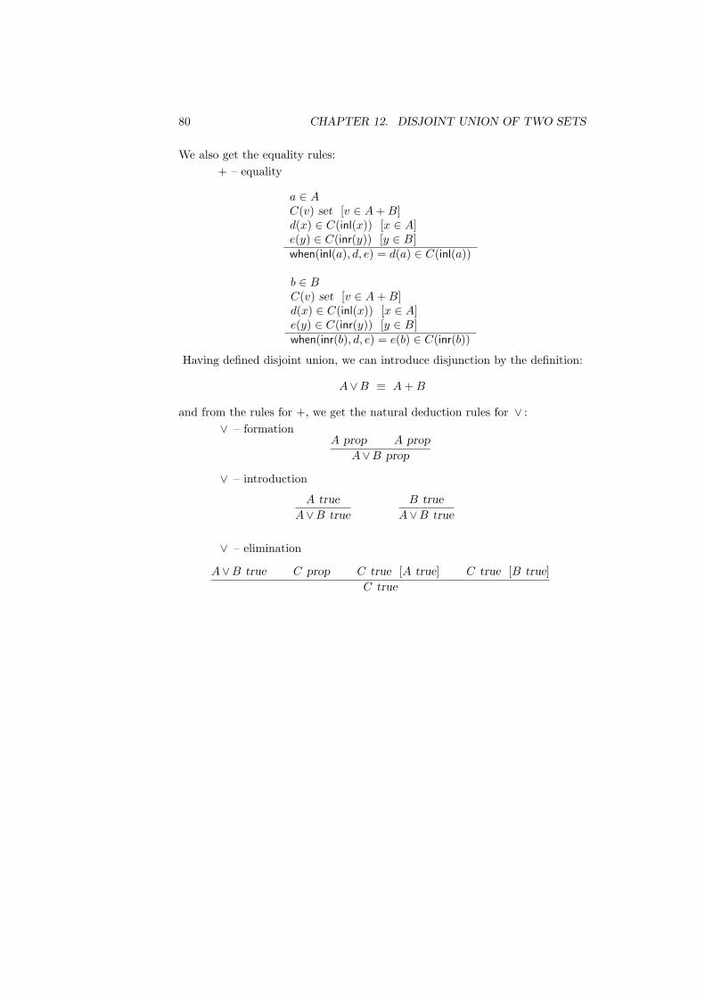
80 CHAPTER 12. DISJOINT UNION OF TWO SETS
We also get the equality rules:+ – equality
a ∈ AC(v) set [v ∈ A + B]d(x) ∈ C(inl(x)) [x ∈ A]e(y) ∈ C(inr(y)) [y ∈ B]when(inl(a), d, e) = d(a) ∈ C(inl(a))
b ∈ BC(v) set [v ∈ A + B]d(x) ∈ C(inl(x)) [x ∈ A]e(y) ∈ C(inr(y)) [y ∈ B]when(inr(b), d, e) = e(b) ∈ C(inr(b))
Having defined disjoint union, we can introduce disjunction by the definition:
A∨B ≡ A + B
and from the rules for +, we get the natural deduction rules for ∨ :∨ – formation
A prop A prop
A∨B prop
∨ – introduction
A true
A∨B true
B true
A∨B true
∨ – elimination
A∨B true C prop C true [A true] C true [B true]C true

Chapter 13
Disjoint union of a family ofsets
In order to be able to deal with the existential quantifier, we will now generalizethe cartesian product of two sets to disjoint union on a family of sets. Wetherefore introduce a new constant Σ of arity 0⊗(0→→0)→→0. Let A be a set andB a family of sets over A, i.e.
B(x) set [x ∈ A]
then we may conclude that Σ(A,B) is a set. So we have the formation ruleΣ – formation
A set B(x) set [x ∈ A]Σ(A,B) set
A canonical element in the set Σ(A,B) is of the form 〈a, b〉 where a is an elementin the set A and b an element in the set B(a). Two canonical elements 〈a, b〉 and〈a′, b′〉 are equal if a = a′ ∈ A and b = b′ ∈ B(a). So we have the introductionrule
Σ – introduction
a ∈ A B(x) set [x ∈ A] b ∈ B(a)〈a, b〉 ∈ Σ(A,B)
We get the cartesian product of two sets if we make the following definition:
A×B ≡ Σ(A, (x)B)
In the chapter on cartesian product of two sets, we introduced the non-canonicalconstant split. The computation rules for split justify the elimination rule
Σ – elimination
c ∈ Σ(A,B)C(v) set [v ∈ Σ(A,B)]d(x, y) ∈ C(〈x, y〉) [x ∈ A, y ∈ B(x)]split(c, d) ∈ C(c)
81

82 CHAPTER 13. DISJOINT UNION OF A FAMILY OF SETS
and the equality ruleΣ – equality
a ∈ Ab ∈ B(a)C(v) set [v ∈ Σ(A,B)]d(x, y) ∈ C(〈x, y〉) [x ∈ A, y ∈ B(x)]split(〈a, b〉, d) = d(a, b) ∈ C(〈a, b〉)
We can show that the elimination rule is correct by assuming the premisesc ∈ Σ(A,B) and d(x, y) ∈ C(〈x, y〉) [x ∈ A, y ∈ B(x)]. The value of split(c, d) iscomputed by first computing c. By the meaning of the first premise, the valueof c is 〈a, b〉 where a ∈ A and b ∈ B(a). The value of split(c, d) is then the valueof d(a, b) which, by the meaning of the second premise and the extensionalityof C, is a canonical element in C(c).
The equality rule is immediately justified from the way split(〈a, b〉, d) is com-puted.
In order to use a notation which is more similar to the existential quantifier,we make the definition
(Σx∈A)B(x) ≡ Σ(A,B)
We can now introduce the existential quantifier:
(∃x∈A)B(x) ≡ (Σx∈A)B(x)
By omitting some of the constructions in the rules for the Σ-set, we get thenatural deduction rules for the existential quantifier:
∃ – introductiona ∈ A B(a) true
(∃x∈A)B(x) true
∃ – elimination
(∃x∈A)B(x) true C prop C true [x ∈ A, B(x) true]C true
Example. All elements in a Σ set are pairs
We will prove that the proposition
(∀p∈Σ(A,B))(∃a∈A)(∃b∈B(a)) (p =Σ(A,B) 〈a, b〉)
is true for an arbitrary set A and an arbitrary family B of sets over A.Assume that p ∈ Σ(A,B). We will prove that the proposition
(∃a∈A)(∃b∈B(a)) (p =Σ(A,B) 〈a, b〉)
is true by Σ-elimination. So, we assume that x ∈ A and y ∈ B(x) and try toprove (∃a ∈A)(∃b ∈B(a)) (〈x, y〉 =Σ(A,B) 〈a, b〉) . But this is immediate fromthe facts that x ∈ A and y ∈ B(x), since then we get that 〈x, y〉 =Σ(A,B) 〈x, y〉 istrue by Id-introduction. And then we can use ∃-introduction twice to concludethat (∃a∈A)(∃b∈B(a)) 〈x, y〉 =Σ(A,B) 〈a, b〉. Finally, we get the desired resultby an ∀-introduction.

Chapter 14
The set of small sets(The first universe)
14.1 Formal rules
The idea behind the set of small sets, i.e. the first universe, is to reflect the setstructure on the object level. In programming we need it for many specificationswhen the most natural way of expressing a proposition is to use recursion orconditionals. We also need it in order to prove inequalities such as 0 6=N succ(0)(see later in this section). It is also necessary when defining abstract data typesin type theory (see chapter 23).
We shall first introduce a set U of small sets, where U is a primitive constantof arity 0, which has constructors corresponding to the set forming operations{i1, ..., in}, N, List, Id, +, Π, Σ, and W. The set forming operation W is usedto represent well-orderings in type theory and is introduced in chapter 15. Westart by introducing the following primitive constants: {i1, ..., in} and N of arity0, List of arity 0→→0, Id of arity 0⊗0⊗0→→0, + of arity 0⊗0→→0 and Π, Σ andW of arity 0⊗(0→→0)→→0.
A problem with the set U is that, because of the enumeration sets, thenumber of constructors is not fixed; this makes it impossible to formulate aninduction principle for U. We will therefore, in section 14.2, change the setstructure and the set of small sets in order to justify an elimination rule forthe universe. One motivation for this is to introduce a selector urec, which isnecessary for doing computations with the elements in the set of small sets.
The set of small sets is defined by giving its canonical elements and theirequality relation. The idea is to let each canonical element represent (code) a setformed by using the set forming operations mentioned earlier. Simultaneouslywith the definition of the canonical elements, we will define a family of setsSet(x) set [x ∈ U] which decodes the elements in the universe to the set theyrepresent. The canonical elements are given by the introduction rules.
U – formationU set
U – introduction 1 {i1, ..., in} ∈ U
83

84 CHAPTER 14. THE SET OF SMALL SETS (THE FIRST UNIVERSE)
Set– introduction 1
Set( {i1, ..., in}) = {i1, ..., in}
U – introduction 2
N ∈ U
Set – introduction 2
Set(N) = N
U – introduction 3
A ∈ U
List(A) ∈ U
Set – introduction 3
A ∈ U
Set(List(A)) = List(Set(A))
U – introduction 4
A ∈ U a ∈ Set(A) b ∈ Set(A)Id(A, a, b) ∈ U
Set – introduction 4
A ∈ U a ∈ Set(A) b ∈ Set(A)Set(Id(A, a, b)) = Id(Set(A), a, b)
U – introduction 5
A ∈ U B ∈ U
A+B ∈ U
Set – introduction 5
A ∈ U B ∈ U
Set(A+B) = Set(A) + Set(B)
U – introduction 6
A ∈ U B(x) ∈ U [x ∈ Set(A)]Π(A,B) ∈ U
Set – introduction 6
A ∈ U B(x) ∈ U [x ∈ Set(A)]Set(Π(A,B)) = Π(Set(A), (x)Set(B(x)))
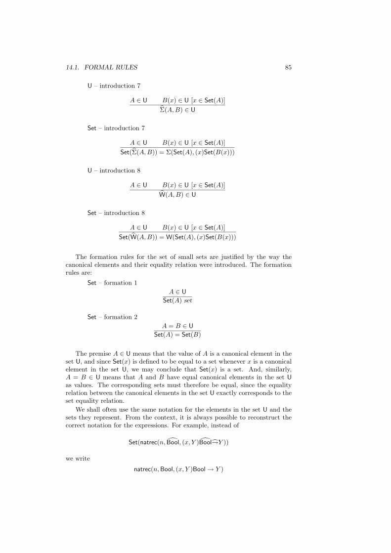
14.1. FORMAL RULES 85
U – introduction 7
A ∈ U B(x) ∈ U [x ∈ Set(A)]Σ(A,B) ∈ U
Set – introduction 7
A ∈ U B(x) ∈ U [x ∈ Set(A)]Set(Σ(A,B)) = Σ(Set(A), (x)Set(B(x)))
U – introduction 8
A ∈ U B(x) ∈ U [x ∈ Set(A)]W(A,B) ∈ U
Set – introduction 8
A ∈ U B(x) ∈ U [x ∈ Set(A)]Set(W(A,B)) = W(Set(A), (x)Set(B(x)))
The formation rules for the set of small sets are justified by the way thecanonical elements and their equality relation were introduced. The formationrules are:
Set – formation 1A ∈ U
Set(A) set
Set – formation 2A = B ∈ U
Set(A) = Set(B)
The premise A ∈ U means that the value of A is a canonical element in theset U, and since Set(x) is defined to be equal to a set whenever x is a canonicalelement in the set U, we may conclude that Set(x) is a set. And, similarly,A = B ∈ U means that A and B have equal canonical elements in the set Uas values. The corresponding sets must therefore be equal, since the equalityrelation between the canonical elements in the set U exactly corresponds to theset equality relation.
We shall often use the same notation for the elements in the set U and thesets they represent. From the context, it is always possible to reconstruct thecorrect notation for the expressions. For example, instead of
Set(natrec(n, Bool, (x, Y )Bool→Y ))
we write
natrec(n, Bool, (x, Y )Bool → Y )

86 CHAPTER 14. THE SET OF SMALL SETS (THE FIRST UNIVERSE)
Example. Peano’s fourth axiom
When we have introduced the universe set we are able to prove that the propo-sition
0 6=N succ(n)
is true for an arbitrary n ∈ N. That is, if we express it in terms of sets, we canconstruct an element peano4 in the set
Id(N, 0, succ(n)) → {}
We will do this by assuming that the set Id(N, 0, succ(n)) is nonempty andshow that we then can construct an element in the empty set. We will usesubstitutivity of propositional equality on a predicate over the natural numberswhich is true only for the number zero.
We start by assuming n ∈ N and x ∈ Id(N, 0, succ(n)). By using N-elimination,we get
natrec(m, T, (y, z){}) ∈ U [m ∈ N]
We make the definition
Is zero(m) ≡ Set(natrec(m, T, (y, z){}))
From N-equality and Set-formation we get the set equalities
Is zero(0) = Set(T) = T
Is zero(succ(n)) = Set({}) = {}
Using substitutivity of propositional equality we get that
subst(x, tt) ∈ Is zero(succ(n))
which by Set-equality yields
subst(x, tt) ∈ {}
Finally, by →-introduction, we discharge the second assumption and obtain
λ((x)subst(x, tt)) ∈ Id(N, 0, succ(n)) → {} [n ∈ N]
So we may putpeano4 ≡ λ((x)subst(x, tt))
and we have a proof of Peano’s fourth axiom.In [101] it is shown that Peano’s fourth axiom cannot be derived in type
theory without universes. The proof is based on interpreting set theory withouta universe in a domain with only two elements. So, a truth valued function ϕ isdefined on the sets and, intuitively, ϕ(A) = > means that the interpretation ofthe set A is a set with one element and ϕ(A) = ⊥ means that A is interpretedas the empty set. ϕ is defined for each set expression A(x1, . . . , xn) by recursion

14.1. FORMAL RULES 87
on the length of the derivation of A(x1, . . . , xn) set [x1 ∈ A1, . . . , xn ∈An(x1, . . . , xn−1)], using the clauses
ϕ({}) = ⊥ϕ({i1, . . . , in}) = >
ϕ(N) = >ϕ(Id(A, a, b)) = ϕ(A)
ϕ(A + B) = ϕ(A) ∨ ϕ(B)ϕ((Πx∈A)B(x)) = ϕ(A) → ϕ(B(x))ϕ((Σx∈A)B(x)) = ϕ(A) ∧ ϕ(B(x))ϕ((Wx∈A)B(x)) = ϕ(A) ∧ (¬ϕ(B(x)))
ϕ({x ∈ A | B(x)}) = ϕ(A) ∧ ϕ(B(x))
Here ∧, ∨, →, and ¬ denote the usual boolean operations.That ϕ really interprets set theory in the intended way is the content of the
following theorem, which is proved in [101].
Theorem Let a(x1, . . . , xn) ∈ A(x1, . . . , xn) be derivable in set theory withoutuniverses under the assumptions x1 ∈ A1, . . . , xn ∈ An(x1, . . . , xn−1). Thenϕ(A(x1, . . . , xn)) = > if ϕ(A1) = · · · = ϕ(An(x1, . . . , xn−1)) = >.
By the interpretation we can now see that for no type A and terms a and bdoes there exist a closed term t such that
t ∈ ¬Id(A, a, b) (∗)
is derivable in type theory without universes. Assume that (∗) holds. Thenthere must exist a derivation of Id(A, a, b) set and, hence, also a derivation ofa ∈ A. So, by the theorem, ϕ(A) = > which, together with the definitions of ϕand ¬, gives
ϕ(¬Id(A, a, b)) = ϕ(Id(A, a, b) → {}) = ϕ(Id(A, a, b)) → ϕ({}) =ϕ(A) → ⊥ = ⊥
Hence, by the theorem, ¬Id(A, a, b) cannot be derived in type theory withoutuniverses.
Assume that Peano’s fourth axiom can be derived, that is, that we, for someclosed term s, have a derivation of
s ∈ (Πx∈N)¬Id(N, 0, succ(x))
By Π-elimination we get apply(s, 0) ∈ ¬Id(N, 0, succ(0)) which is of the form (∗)and therefore impossible to derive in type theory without universes.
Example. The tautology function
A disadvantage with many type systems in programming languages is that someexpressions, although perfectly reasonable, can not be assigned a type. Thetype systems are not well suited to express some properties needed for a safeevaluation of the expression. As an example, take the tautology function from

88 CHAPTER 14. THE SET OF SMALL SETS (THE FIRST UNIVERSE)
the SASL manual [110]. It determines if a boolean expression of n variables(represented as a curried function of n arguments) is a tautology or not. Thefunction is defined, using SASL-notation, as:
taut 0 f = f
taut n f = taut(n− 1) (f true) and taut(n− 1) (f false)
Since SASL is untyped, the function is not assigned a type and for most othertyped languages the definition causes a type error. Informally the type of tautis
(Πn ∈ N)((Bool →n Bool) → Bool)
where (Bool →n Bool) is defined by the equations
Bool →0 Bool = Bool
Bool →k+1 Bool = Bool → (Bool →k Bool)
So, for example,
taut 0 ∈ Bool → Bool
taut 3 ∈ (Bool → Bool → Bool → Bool) → Bool
and we can see that the type of the second argument depends on the value ofthe first.
The type of taut can be expressed using the set U in type theory. Make thefollowing definitions:
and(x, y) ≡ if x then y else false
F(n) ≡ natrec(n, Bool, (x, Y )Bool → Y )taut(n) ≡ natrec(n,
λ((f)f),(x, y)λ((f)and(y · (f · true),
y · (f · false))))
Notice that we have used the infix version of the constant apply,
x · y ≡ apply(x, y)
From these definitions, it immediately follows that
and(x, y) ∈ Bool [x ∈ Bool, y ∈ Bool] (14.1)F(0) = Bool ∈ U (14.2)F(succ(x)) = Bool → F(x) ∈ U [x ∈ N] (14.3)
Using Set-formation on (14.2) and (14.3), we get the set equalities
F(0) = Bool (14.4)F(succ(x)) = Bool → F(x) [x ∈ N] (14.5)
The goal is to prove:
λ((n)taut(n)) ∈ (Πn ∈ N)(F(n) → Bool)

14.1. FORMAL RULES 89
so we start by assuming thatn ∈ N
and then prove taut(n) ∈ F(n) → Bool by induction on n. We first have thebase case. It is easy to see that
λ((f)f) ∈ Bool → Bool
and, since we from (14.4) and →-formation get the set equality
F(0) → Bool = Bool → Bool
we can conclude thatλ((f)f) ∈ F(0) → Bool (14.6)
For the induction step, we make the assumptions
x ∈ N
y ∈ F(x) → Bool
The goal is to prove
λ((f)and(y · (f · true), y · (f · false))) ∈ F(succ(x)) → Bool
We therefore make the assumption
f ∈ F(succ(x)) (14.7)
From (14.7) and the set equality (14.4), we get
f ∈ Bool → F(x)
and then by →-elimination
f · true ∈ F(x)f · false ∈ F(x)
and furthermore by using the induction hypothesis
y · (f · true) ∈ Bool
y · (f · false) ∈ Bool
By substituting these elements into (14.1), we obtain
and(y · (f · true), y · (f · false))) ∈ Bool
By →-introduction, we discharge assumption (14.7) and get
λ((f)and(y · (f · true), y · (f · false))) ∈ F(succ(x)) → Bool (14.8)
We can now use N-elimination on (14.6) and (14.8) to obtain
taut(n) ∈ F(n) → Bool
and finally, by Π-introduction, we get the desired result
λ((n)taut(n)) ∈ (Πn ∈ N)(F(n) → Bool)

90 CHAPTER 14. THE SET OF SMALL SETS (THE FIRST UNIVERSE)
Example. An expression without normal form in the the-ory with extensional equality
A canonical element in the set (Πx∈A)B(x) is of the form λ(b) where b(x) ∈B(x) [x ∈ A] and the expression b(x) is not further evaluated. We have alreadyremarked that evaluating b(x) would be the same as trying to execute a programwhich expects an input without giving any input. Using the extensional equalityEq and the universe in a crucial way, we will now give an example of a lambda-expression λ(b) in the set {} → A, where, by regarding the evaluation rules asreduction rules, b(x) does not even terminate.
By the use of the set of small sets, we will show that
Set(A) = Set(B) [A ∈ U, B ∈ U, x ∈ {}] (14.1)
Assumex ∈ {}
Since Eq(U, A, B) is a set, we get by {}-elimination that
case0(x) ∈ Eq(U, A, B) [A ∈ U, B ∈ U, x ∈ {}]
and by strong Eq-elimination it follows that
A = B ∈ U [A ∈ U, B ∈ U, x ∈ {}] (14.2)
Set-formation 2 and (2) gives
Set(A) = Set(B) [A ∈ U, B ∈ U, x ∈ {}]
and, hence, we have a derivation of (1).Now assume
x ∈ {} (14.3)
By choosing A to be N and B to be N→N, we get from (1)
N = N → N (14.4)
Assumey ∈ N (14.5)
One of the rules for set equality applied on (4) and (5) gives
y ∈ N → N (14.6)
From (5) and (6) we get, by →-elimination,
apply(y, y) ∈ N (14.7)
and from (7) we get, by →-introduction,
λy.apply(y, y) ∈ N → N (14.8)
thereby discharging the assumption (5). (6) and (8) give
λy.apply(y, y) ∈ N (14.9)

14.2. ELIMINATION RULE 91
We can now apply →-elimination on (8) and (9) to get
apply(λy.apply(y, y), λy.apply(y, y)) ∈ N
and →-introduction finally gives
λx.apply(λy.apply(y, y), λy.apply(y, y)) ∈ {} → N
thereby discharging the assumption (3). The expression
apply(λy.apply(y, y), λy.apply(y, y))
is the well-known example from combinatory logic of an expression which re-duces to itself. Since this expression is not on canonical form, we have anexample of a lambda-expression which is an element of a Π-set and whose bodydoes not terminate. Notice that there is no violation of the arity rules whenforming apply(y, y) because apply is of arity 0⊗0→→0 and y is a variable of arity0.
14.2 Elimination rule
With a set of small sets that reflects a set structure with infinitely many setforming operations, it is impossible to justify a structural induction rule onthe set. In order to be able to introduce such an induction rule, the smallenumeration sets, i.e the sets {i1, ..., in}, must be generated from finitely manybasic enumeration sets. We shall therefore modify the system of set formingoperations, and consequently also the set of small sets, to make room for aninduction rule on the elements of the universe. The modified system will onlycontain two basic enumeration sets, the empty set and a set with one element(see the section on enumeration sets); the other enumeration sets are generatedfrom these two sets by means of the disjoint union. With a set structure withonly these two enumeration sets, we get a set of small sets where the first U-introduction rule is replaced by the rules:
U – introduction 1a
∅ ∈ U
Set(∅) = ∅
andU – introduction 1b
T ∈ U
Set(T) = T
An enumeration set with more than one element is formed by repeated use ofthe T set and the disjoint union. We introduce the function constant N′ of arity0 by the definition:
N′(x) ≡ natrec(x, ∅, (u, v)S′(v))
where

92 CHAPTER 14. THE SET OF SMALL SETS (THE FIRST UNIVERSE)
S′(x) ≡ T+x
SoSet(S′(A)) set [A ∈ U] (14.10)
and N′ applied to a natural number n gives an element in U, which correspondsto an enumeration set with n elements. We can now prove that
N′(x) ∈ U [x ∈ N] (14.11)N′(succ(x)) = S′(N′(x)) ∈ U [x ∈ N] (14.12)
From 14.11, we get, by Set-formation,
Set(N′(x)) set [x ∈ N]
Moreover, simplification gives us:
Set(N′(0)) = ∅Set(N′(1)) = T + ∅
with the element inl(tt), and
Set(N′(2)) = T+(T+∅)
with elements inl(tt) and inr(inl(tt)), and so on. If the enumeration sets de-fined here are compared with the enumeration sets Nk in [69] then Set(N′(k))corresponds to Nk, inl(tt) corresponds to 0k and inr(inr(. . . inr(inl(tt)) . . .)) cor-responds to nk, with n being the number of ‘inr’-applications.
By making the definitions:
o′ ≡ inl(tt)s′(x) ≡ inr(x)
scase′(x, y, z) ≡ when(x, (w)y, z)
where o′, s′ and scase′ are constants of arity 0, 0→→0 and 0⊗0⊗(0→→0)→→0respectively, we can prove the judgements
o′ ∈ Set(S′(A)) [A ∈ U] (14.13)
s′(x) ∈ Set(S′(A)) [A ∈ U, x ∈ Set(A)] (14.14)
scase′(x, y, z) ∈ Set(C(x))[A ∈ U, x ∈ Set(S′(A)), C(u) ∈ U [u ∈ Set(S′(A))],y ∈ Set(C(o′)), z(v) ∈ C(s′(v)) [v ∈ Set(A)]]
(14.15)
scase′(o′, y, z) = y ∈ Set(C(o′))[A ∈ U, C(u) ∈ U [u ∈ Set(S′(A))],y ∈ Set(C(o′)), z(v) ∈ C(s′(v)) [v ∈ Set(A)]]
(14.16)
scase′(s′(x), y, z) = z(x) ∈ Set(C(s′(x)))[A ∈ U, x ∈ Set(A), C(u) ∈ U [u ∈ Set(S′(A))],y ∈ Set(C(o′)), z(v) ∈ C(s′(v)) [v ∈ Set(A)]]
(14.17)

14.2. ELIMINATION RULE 93
Per Martin-Lof has given a more direct formulation of the enumerationsets by introducing the set former S as a primitive constant with the follow-ing rules (compare with the theorems (14.10), (14.13), (14.14), (14.15), (14.16)and (14.17) above):
S– formationA set
S(A) set
S– introduction
o ∈ S(A)a ∈ A
s(a) ∈ S(A)
S– elimination
a ∈ S(A) b ∈ C(o) c(x) ∈ C(s(x)) [x ∈ A]scase(a, b, c) ∈ C(a)
S– equality
b ∈ C(o) c(x) ∈ C(s(x)) [x ∈ A]scase(o, b, c) = b ∈ C(o)
a ∈ S(A) b ∈ C(o) c(x) ∈ C(s(x)) [x ∈ A]scase(s(a), b, c) = c(a) ∈ C(s(a))
Given the reformulated set of small sets, we can now justify a structuralinduction rule, which is introduced as follows. First we introduce urec as aconstant of arity
0⊗0⊗0⊗0⊗
(0⊗0→→0)⊗(0⊗0⊗0⊗0→→0))⊗(0⊗0⊗0⊗0→→0))⊗(0⊗(0→→0)⊗0⊗(0→→0)→→0)⊗(0⊗(0→→0)⊗0⊗(0→→0)→→0)⊗(0⊗(0→→0)⊗0⊗(0→→0)→→0)
→→0
and we then define how urec(A, a1, . . . , a9) is computed by the following rules(a ⇒ b means that b is the value of a).
a ⇒ ∅ a1 ⇒ b
urec(a, a1, a2, a3, a4, a5, a6, a7, a8, a9) ⇒ b
a ⇒ T a2 ⇒ b
urec(a, a1, a2, ..., a9) ⇒ b
a ⇒ N a3 ⇒ b
urec(a, a1, a2, ..., a9) ⇒ b

94 CHAPTER 14. THE SET OF SMALL SETS (THE FIRST UNIVERSE)
a ⇒ List(A) a4(A, urec(A, a1, a2, ..., a9)) ⇒ b
urec(a, a1, a2, ..., a9) ⇒ b
a ⇒ Id(A, c, d) a5(A, c, d, urec(A, a1, ..., a9)) ⇒ b
urec(a, a1, a2, ..., a9) ⇒ b
a ⇒ A+B a6(A,B, urec(A, a1, ..., a9), urec(B, a1, ..., a9)) ⇒ b
urec(a, a1, a2, ..., a9) ⇒ b
a ⇒ Π(A,B) a7(A,B, urec(A, a1, ..., a9), (w)urec(B(w), a1, ..., a9)) ⇒ b
urec(a, a1, a2, ..., a9) ⇒ b
a ⇒ Σ(A,B) a8(A,B, urec(A, a1, ..., a9), (w)urec(B(w), a1, ..., a9)) ⇒ b
urec(a, a1, a2, ..., a9) ⇒ b
a ⇒ W(A,B) a9(A,B, urec(A, a1, ..., a9), (w)urec(B(w), a1, ..., a9)) ⇒ b
urec(a, a1, a2, ..., a9) ⇒ b
A restriction in these rules is that w must not occur free in B, a1,. . . , a8 or a9.It would otherwise be bound in (w)urec(B(w), a1, ..., a9).
The computation rule for urec justifies the following elimination rule for theset of small sets:
U- elimination
a ∈ UC(v) set [v ∈ U]a1 ∈ C(∅)a2 ∈ C(T)a3 ∈ C(N)a4(x, y) ∈ C(List(x)) [x ∈ U, y ∈ C(x)]a5(x, y, z, u) ∈ C(Id(x, y, z)) [x ∈ U, y ∈ Set(x), z ∈ Set(x), u ∈ C(x)]a6(x, y, z, u) ∈ C(x+y) [x ∈ U, y ∈ U, z ∈ C(x), u ∈ C(y)]a7(x, y, z, u) ∈ C(Π(x, y)) [x ∈ U, y(v) ∈ U[v ∈ Set(x)],
z ∈ C(x), u(v) ∈ C(y(v))[v ∈ Set(x)]]a8(x, y, z, u) ∈ C(Σ(x, y)) [x ∈ U, y(v) ∈ U[v ∈ Set(x)],
z ∈ C(x), u(v) ∈ C(y(v))[v ∈ Set(x)]]a9(x, y, z, u) ∈ C(W(x, y)) [x ∈ U, y(v) ∈ U[v ∈ Set(x)],
z ∈ C(x), u(v) ∈ C(y(v))[v ∈ Set(x)]]urec(a, a1, a2, a3, a4, a5, a6, a7, a8, a9) ∈ C(a)
Here x, y, z and u must not occur free in the abstraction C. In the followingrules we will not write down the premise C(v) set [v ∈ U].
We also have an elimination rule where the premises and conclusion are ofthe form a = b ∈ A. Furthermore, the computation rule for urec justifies thefollowing equality rules. The last 9 premises of all the equality rules are thesame as the last 9 premises of the elimination rule above.
U- equality 1
a1 ∈ C(∅) a2 ∈ C(T) . . . a9(x, y, z, u) ∈ C(W(x, y)) [. . .]urec(∅, a1, a2, a3, a4, a5, a6, a7, a8, a9) = a1 ∈ C(∅)

14.2. ELIMINATION RULE 95
U- equality 2
a1 ∈ C(∅) a2 ∈ C(T) . . . a9(x, y, z, u) ∈ C(W(x, y)) [. . .]urec(T, a1, a2, a3, a4, a5, a6, a7, a8, a9) = a2 ∈ C(T)
U- equality 3
a1 ∈ C(∅) a2 ∈ C(T) . . . a9(x, y, z, u) ∈ C(W(x, y)) [. . .]urec(N, a1, a2, a3, a4, a5, a6, a7, a8, a9) = a3 ∈ C(N)
U- equality 4
A ∈ U a1 ∈ C(∅) . . . a9(x, y, z, u) ∈ C(W(x, y)) [. . .]urec(List(A), a1, . . . , a9) = a4(A, urec(A, a1, . . . , a9)) ∈ C(List(A))
U- equality 5
A ∈ Uc ∈ Set(A)d ∈ Set(A) a1 ∈ C(∅)
...a9(x, y, z, u) ∈ C(W(x, y)) [. . .]urec(Id(A, c, d), a1, . . . , a9) =a5(A, c, d, urec(A, a1, . . . , a9)) ∈ C(Id(A, c, d))
U- equality 6
A ∈ UB ∈ U
a1 ∈ C(∅)...
a9(x, y, z, u) ∈ C(W(x, y)) [. . .]urec(A+B, a1, . . . , a9) =a6(A,B, urec(A, a1 . . . , a9), urec(B, a1, . . . , a9)) ∈ C(A+B)
U- equality 7
A ∈ UB(x) ∈ U [x ∈ Set(A)]a1 ∈ C(∅)
...a9(x, y, z, u) ∈ C(W(x, y)) [. . .]urec(Π(A,B), a1, . . . , a9) =a7(A,B, urec(A, a1, . . . , a9), (w)urec(B(w), a1, . . . , a9)) ∈ C(Π(A,B))

96 CHAPTER 14. THE SET OF SMALL SETS (THE FIRST UNIVERSE)
U- equality 8
A ∈ UB(x) ∈ U [x ∈ Set(A)]a1 ∈ C(∅)
...a9(x, y, z, u) ∈ C(W(x, y)) [. . .]urec(Σ(A,B), a1, . . . , a9) =a8(A,B, urec(A, a1, . . . , a9), (w)urec(B(w), a1, . . . , a9)) ∈ C(Σ(A,B))
U- equality 9
A ∈ UB(x) ∈ U [x ∈ Set(A)]a1 ∈ C(∅)
...a9(x, y, z, u) ∈ C(W(x, y)) [. . .]urec(W(A,B), a1, . . . , a9) =a9(A,B, urec(A, a1, . . . , a9), (w)urec(B(w), a1, . . . , a9)) ∈ C(W(A,B))
The variables x, y, z and u must not occur free in C, and there must be nofree occurrences of w in B, a1, . . . or a9.

Chapter 15
Well-orderings
In order to introduce the well-ordering set constructor (or well-founded tree setconstructor) we introduce the primitive constants
W of arity (0⊗(0→→0))→→0sup of arity (0⊗(0→→0))→→0
wrec of arity 0⊗(0⊗(0→→0)⊗(0→→0)→→0)→→0
With the well-order set constructor we can construct many different sets oftrees and to characterize a particular set we must provide information abouttwo things:
• the different ways the trees may be formed, and
• for each way to form a tree which parts it consists of.
To provide this information, the well-order set constructor W has two arguments:
1. The constructor set A.
2. The selector family B.
Given a constructor set A and selector family B on A, we can form a well-orderW(A,B) (two other notations are (Wx∈A)B(x) and Wx∈AB(x)). The formationrule therefore has the following form:
W - formation
A set B(x) set [x ∈ A]W(A,B) set
The elements in the set A represents the different ways to form an element inW(A,B) and B(x) represents the parts of a tree formed by x.
The elements of a well-order W(A,B) can, as we already mentioned, be seenas well-founded trees and to form a particular element of W(A,B) we must saywhich way the tree is formed and what the parts are. If we have an element a inthe set A, that is, if we have a particular form we want the tree to have, and if wehave a function from B(a) to W(A,B), that is if we have a collection of subtrees,we may form the tree sup(a, b). We visualize this element in figure 15.1. Theintroduction rule has the form
97

98 CHAPTER 15. WELL-ORDERINGSs sup(a1, b1) ∈ W(A,B)�
��
��
��
��
��
��
��
@@
@@
@@
@@
@@
@@
@@@
%%
%%
%%
%%
%
c1 ∈ B(a1)
. . .
b1(c1) = sup(a2, b2)∈ W(A,B)
s�
��
��
@@
@@
@
��
�s�� SS
SSSs�� SS
JJ
JJ
JJ
JJJs
��
��
�
@@
@@
@
Figure 15.1: An element of a well-order
W - introductiona ∈ A b(x) ∈ W(A,B) [x ∈ B(a)]
sup(a, b) ∈ W(A,B)
It may seem strange that we do not have a particular introduction rule forthe leaves, but we get the same effect if we choose B(x) to be the empty set forsome x ∈ A. In the introduction rule we can see that we must provide a functionfrom B(x) to W(A,B) in order to form an element sup(a, b). In the case whenB(x) is the empty set, we use a small “trick” to provide such a function. Fromthe assumption x ∈ {}, we can, by using the {}-elimination rule, conclude thatcase{}(x) is an element of an arbitrary set, and in this case we of course chooseW(A,B). So if B(a) is empty, then (x)case{}(x) ≡ case{} is a function fromB(a) to W(A,B) and sup(a, case{}) is an element of W(A,B).
Let us take a simple example. We want to construct a well-order set torepresent simple binary trees which, for example, could be defined in ML [72]by
datatype BinTree = leaf | node of BinTree ∗ BinTree
There are two different ways of constructing a binary tree, one to constructa leaf and one to construct a compound tree. The constructor set A musttherefore contain two elements, and we can for example use the enumerationset {leaf,node}. A leaf does not have any parts, so B(leaf) must be the emptyset, and a compound tree has two parts, so we can choose B(node) as the set{left, right}. Putting this together, we get a well-order set
BinTree ≡ W({leaf,node}, (x)Set(case{leaf,node}(x, {}, {left, right})))
which has representations of all binary trees as elements. Notice that we mustuse the universe set to construct the family B. The elements of this well-orderare always of one of the forms
sup(leaf, case{}) sup(node, (x)case{left,right}(x, t′, t′′))
where t′ and t′′ are two elements in W(A,B). By introducing definitions
leaf′ ≡ sup(leaf, case)node′(t′, t′′) ≡ sup(node, (x)case(x, t′, t′′))

99
we get expressions for the elements that look just like the corresponding MLexpressions.
The non-canonical constant in a well-ordering is wrec and the expressionwrec(a, b) is computed as follows:
1. Compute the value of a.
2. If the value is sup(d, e), then the value of wrec(a, b) is the value ofb(d, e, (x)wrec(e(x), b)).
The computation rule for wrec justifies the following elimination rule:W – elimination
a ∈ W(A,B)C(v) set [v ∈ W(A,B)]b(y, z, u) ∈ C(sup(y, z))
[y ∈ A, z(x) ∈ W(A,B) [x ∈ B(y)], u(x) ∈ C(z(x)) [x ∈ B(y)]]wrec(a, b) ∈ C(a)
and the following equality ruleW - equality
d ∈ Ae(x) ∈ W(A,B) [x ∈ B(d)]C(v) set [v ∈ W(A,B)]b(y, z, u) ∈ C(sup(y, z))
[y ∈ A, z(x) ∈ W(A,B) [x ∈ B(y)], u(x) ∈ C(z(x)) [x ∈ B(y)]]wrec(sup(d, e), b) = b(d, e, (x)wrec(e(x), b)) ∈ C(sup(d, e))
As an example of how the non-canonical constant can be used, we define thefunction that counts the number of nodes in a binary tree and which in MLcould be defined by:
fun nrofnodes(leaf) = 1| nrofnodes(node(t′, t′′)) = nrofnodes(t′) + nrofnodes(t′′)
In type theory this function could be defined by
nrofnodes(x) ≡ wrec(x, (y, z, u)case(y, 1, u(left) + u(right)))
Using the elimination rule, we immediately see that
nrofnodes(x) ∈ N [x ∈ BinTree]
and using the equality rule, we immediately get the equalities that correspondto the ML definition.
In the same way as we above introduced defined constants to get a nicersyntax for the elements of the type BinTree, we can make a definition and geta constant that behaves just like a recursion operator on binary trees.
trec′(t, a, b) ≡ wrec(t, (x, y, z)case(x, a, b(y(left), y(right), z(left), z(right))))
The equality rule for wrec corresponds to the equalities:
trec′(leaf′, a, b) = a
trec′(node′(t′, t′′), a, b) = b(t′, t′′, trec′(t′, a, b), trec′(t′′, a, b))

100 CHAPTER 15. WELL-ORDERINGS
And the function counting the number of nodes, which we defined above, canthen be defined as
nrofnodes ≡ trec′(x, 1, (t′, t′′, z′, z′′) z′⊕z′′)
Example. Defining the natural numbers as a well-ordering
It is not difficult to see that the set of natural numbers can be defined by thefollowing abbreviations:
N ≡ (Wx ∈ {zero, succ})Set(case(x, {}, T))0 ≡ sup(zero, case)
succ(a) ≡ sup(succ, (x)a)natrec(a, b, c) ≡ wrec(a, (y, z, u)case(y, b, c(z(tt), u(tt)))
The idea is to let the n:th natural number be represented by a thin tree of heightn. We immediately see from the W-formation rule that
(Wx ∈ {zero, succ}) Set(case(x, {}, T)) set
and therefore, using the definition of N, that the formation rule for the naturalnumbers can be proved. We can also see, by using the W-introduction rule, that
sup(zero, case) ∈ (Wx ∈ {zero, succ})Set(case(x, {}, T))
and hence, using the abbreviations, that the first N-introduction rule, 0 ∈ N,holds. The second introduction rule, succ(x) ∈ N [x ∈ N], corresponds to thejudgement
sup(succ, (y)x) ∈ (Wx ∈ {zero, succ})Set(case(x, {}, T))[x ∈ (Wx ∈ {zero, succ})Set(case(x, {}, T))]
which also is proved directly from the W-introduction rule.Unfortunately the N-elimination rule and the N-equality rule can not be
proved using the intensional equality in type theory. The reason for this isthat there are more elements in the well-order representing the natural numbersthan one expect at first. An element sup(a, b) of a well-order has a functionalcomponent b and the intensional equality means that two functions are equalonly if they convert to each other. So the two functions
(x) 0 and (x) 1
which maps elements in the empty set to natural numbers are not equal evenif they give the same result for all elements in the domain. The consequenceof this for the representation of natural numbers is that there are elements inthe well-order that do not represent any natural number. With an extensionalequality this problem never occurs.

15.1. REPRESENTING INDUCTIVELY DEFINED SETS BY WELL-ORDERINGS101
15.1 Representing inductively defined sets bywell-orderings
Most programming languages have some construction for defining types by in-ductive definitions. “Old” languages use pointers and records and “modern”languages use more sophisticated constructions, see for example [51] and [72].In type theory the well-order set constructor can be used for representing manyinductively defined sets. But as we remarked above, we must have an extensionalequality in order to get the correct elimination and equality rules.
We have shown above how one could represent binary trees and natural num-bers by well-orders. Let us also show how one can define an inductively definedset which uses another set in its definition. Consider the set of binary trees withnatural numbers in its nodes and defined by the following ML definition
datatype BinTree = leaf of N | node of N ∗ BinTree ∗ BinTree
In order to represent this set by a well-order one must consider the naturalnumber as part of the constructor of the tree and instead of having a twoelement set as the set of constructors, we now need N × N. The selectors forinl(n) is the empty set and for inr(n) the set {left, right}. So
W(N + N, (x)Set(when(x, (n){}, (n) {left, right})))
is a well-ordering that represents the type of binary trees with natural numbersin its nodes. The elements are of the form
sup(inl(n), case) and sup(inr(n), (x)case(x, t′, t′′))
where n is a natural number and t′ and t′′ are two elements in W(A,B). To geta better syntax, we can introduce three definitions:
leaf′′(n) ≡ sup(inl(n), case)node′′(n, t′, t′′) ≡ sup(inr(n), (x)case(x, t′, t′′))
trec′′(t, a, b) ≡ wrec(t,(y, z, u)when(y, a, (n)b(n,
z(left),z(right),u(left), u(right))))
The function that adds all the numbers in a tree could in type theory be definedby
addnum(x) ≡ trec′′(x, (n)n, (n, y, z, u, v)n + u + v)≡ wrec(x, (y, z, u)when(y, (n)n, (n)n + u(left) + u(right))

102 CHAPTER 15. WELL-ORDERINGS

Chapter 16
General trees
When we introduced the well-order set constructor in the previous chapter, wesaid that many inductively defined sets could be represented by well-orders andthat the elements of a well-order could be seen as well-founded trees. The well-order set constructor, however, is not easy to use when we want to define afamily of mutually dependent inductive sets, or mutually dependent families oftrees.
For example if we want to represent the types defined in ML by
datatype Odd = sO of Evenand Even = zeroE | sE of Odd;
it is possible but quite complicated to do this by using well-orders. We thereforeintroduce a set constructor, Tree, which could be used for representing such setsin a more direct way. Notice that we must have an extensional equality to getthe correct elimination and equality rule when we represent inductively definedtypes by well-orders and general trees. The set constructor for general trees wasfirst introduced in [88] on which the following chapter is based.
The constructor should produce a family of sets instead of one set as thewell-order set constructor does. In order to do this, we introduce a name set,which is a set of names of the mutually defined sets in the inductive definition.A suitable choice of name set for the example above would be {Odd, Even}.Instead of having one set of constructors B and one index family C over B, asin the well-order case, we now have one constructor set and one selector familyfor each element in A. The constructors form a family of sets B, where B(x)is a set for each x in A and the selector family forms a family of sets C whereC(x, y) is a set for each x in A and y in B(x). Furthermore, since the partsof a tree now may come from different sets, we introduce a function d whichprovides information about this; d(x, y, z) is an element of A if x ∈ A, y ∈ B(x)and z ∈ C(x, y). We call this element the component set name.
The family of sets Tree(A,B, C, d) is a representation of the family of setsintroduced by a collection of inductive definitions, for example an ML data typedefinition. It could also be seen as a solution to the equation
T ∼= (x)(Σy ∈ B(x))(Πz ∈ C(x, y))T (d(x, y, z))
where T is a family of sets over A and x ∈ A. This equation could be interpreted
103

104 CHAPTER 16. GENERAL TREES
as a possibly infinite collection of ordinary set equations, one for each a ∈ A.
T (a1) ∼= (Σy ∈ B(a1))(Πz ∈ C(a1, y)) T (d(a1, y, z))T (a2) ∼= (Σy ∈ B(a2))(Πz ∈ C(a2, y)) T (d(a2, y, z))
...
Or, if we want to express the tree set constructor as the least fixed point of aset function operator.
Tree(A,B,C, d) ∼= FIX((T )(x)(Σy ∈ B(x))(Πz ∈ C(x, y)) T (d(x, y, z)))
Comparing this equation with the equation for the well-order set constructor
W(B,C) ∼= FIX((X )(Σy ∈ B)C(y) → X )
we can see that it is a generalization in that the non-dependent function set,“→”, has become a set of dependent functions, Π. This is a natural general-ization since we are now defining a family of sets instead of just one set andevery instance of the family could be defined in terms of every one of the otherinstances. It is the function d that expresses this relation.
16.1 Formal rules
In order to be able to formulate the rules for the set constructor for trees, weintroduce the primitive constant Tree which has the arity
0⊗(0→→0)⊗(0⊗0→→0)⊗(0⊗0⊗0→→0)→→0→→0
tree of arity 0⊗(0→→0)→→0 and finally treerec of arity
0⊗(0⊗(0→→0)⊗(0→→0)→→0)→→0
The formation rule for the set of trees is:Tree – formation
A setB(x) set [x ∈ A]C(x, y) set [x ∈ A, y ∈ B(x)]d(x, y, z) ∈ A [x ∈ A, y ∈ B(x), z ∈ C(x, y)]a ∈ A
Tree(A,B,C, d)(a) set
The different parts have the following intuitive meaning:
• A, the name set, is a set of names for the mutually dependent sets.
• B(x), the constructor set, is a set of names for the clauses defining the setx.
• C(x, y), the selector family, is a set of names for selectors of the parts inthe clause y in the definition of x.

16.1. FORMAL RULES 105
• d(x, y, z), the component set name, is the name of the set correspondingto the selector z in clause y in the definition of x.
• a determines a particular instance of the family of sets.
Understood as a set of syntax-trees generated by a grammar, the differentparts have the following intuitive meaning:
• A is a set of non-terminals.
• B(x) is a set of names for the alternatives defining the non-terminal x.
• C(x, y), is a set of names for positions in the sequence of non-terminals inthe clause y in the definition of x.
• d(x, y, z), is the name of the non-terminal corresponding to the position zin clause y in the definition of x.
• a is the start symbol.
In order to reduce the notational complexity, we will write T (a) instead ofTree(A,B, C, d)(a) in the rest of this chapter.
The introduction rule for trees has the following formTree – introduction
a ∈ Ab ∈ B(a)c(z) ∈ T (d(a, b, z)) [z ∈ C(a, b)]
tree(a, b, c) ∈ T (a)
Intuitively:
• a is the name of one of the mutually dependent sets.
• b is one of the constructors of the set a.
• c is a function from C(a, b) to a tree. This function defines the differentparts of the element.
The element tree(a, b, c) in the set T (a) corresponds to the tree in figure 16.1,where C(a, b) = {z1, . . . , zn, . . .} and c(zi) ∈ T (d(a, b, zi)).
The elimination rule has the formTree – elimination
D(x, t) set [x ∈ A, t ∈ T (x)]a ∈ At ∈ T (a)f(x, y, z, u) ∈ D(x, tree(x, y, z))
[x ∈ A, y ∈ B(x), z(v) ∈ T (d(x, y, v)) [v ∈ C(x, y)],u(v) ∈ D(d(x, y, v), z(v)) [v ∈ C(x, y)]]
treerec(t, f) ∈ D(a, t)
Its correctness follows from the computation rule for the non-canonical constanttreerec which says that the expression treerec(d, e) is computed as follows

106 CHAPTER 16. GENERAL TREESs tree(a, b, c) ∈ T (a)�
��
��
��
��
��
��
��
@@
@@
@@
@@
@@
@@
@@@
%%
%%
%%
%%
%
z ∈ C(a, b)
. . .
c(z) = tree(a′, b′, c′)∈ T (d(a, b, z))︸ ︷︷ ︸
a′
s�
��
��
@@
@@
@
��
�s�� SS
SSSs�� SS
JJ
JJ
JJ
JJJs
��
��
�
@@
@@
@
Figure 16.1: An element in the set Tree(A,B, C, d)(a)
1. Evaluate d to canonical form.
2. If the value of d is tree(a, b, c) then the value of the expression is e(a, b, c, (x)treerec(c(x), d)).
The computation rule is also reflected in the equality rule:Tree-equality
D(x, t) set [x ∈ A, t ∈ T (x)]a ∈ Ab ∈ B(a)c(z) ∈ T (d(a, b, z)) [z ∈ C(a, b)]f(x, y, z, u) ∈ D(x, tree(x, y, z))
[x ∈ A, y ∈ B(x), z(v) ∈ T (d(x, y, v)) [v ∈ C(x, y)],u(v) ∈ D(d(x, y, v), z(v)) [v ∈ C(x, y)]]
treerec(tree(a, b, c), f) = f(a, b, c, (x)treerec(c(x), f)) ∈ D(a, tree(a, b, c))
16.2 Relation to the well-order set constructor
A well-order set W(B,C) can be seen as an instance of a Tree set. We get thewell-orders by defining a family of trees on a set with only one element. If wemake the definitions:
W(B,C) = Tree(T, (x)B, (x, y)C(y), (x, y, z)tt, tt)sup(b, c) = tree(tt, b, c)
wrec(t, f) = treerec(t, (x, y, z, u)f(y, z, u))
where T is the set consisting of the element tt. Then we can derive the rules forwell-orders from the rules for trees as follows:
Formation rule: If we assume that the premises of the well-order formationrule hold, that is, if we assume
B setC(y) set [y ∈ B]

16.2. RELATION TO THE WELL-ORDER SET CONSTRUCTOR 107
we can infer
T set((x)B)(x) set [x ∈ T]((x, y)C(y))(x, y) set [x ∈ T, y ∈ B]((x, y, z)tt)(x, y, z) ∈ T [x ∈ T, y ∈ B, z ∈ C(y)]tt ∈ T
and then, by the Tree-formation rule, get
Tree(T, (x)B, (x, y)C(y), (x, y, z)tt, tt) set
which is the same as
W(B,C) set
and also the conclusion of the formation rule. So we have proved thatthe formation rule holds for the definition of well-orders in terms oftrees.
Introduction rule: Assume
b ∈ Bc(z) ∈ W(B,C) [z ∈ C(b)]
From the last assumption we get
c(z) ∈ Tree(T, (x)B, (x, y)C(y), (x, y, z)tt, tt) [z ∈ C(b)]
It then follows that
tt ∈ Tb ∈ ((x)B)(tt)c(z) ∈ Tree(T, (x)B, (x, y)C(y), (x, y, z)tt, ((x, y, z)tt))(tt, b, z)
[z ∈ ((x, y)C(y))(b)]
and, from the Tree-introduction rule,
tree(tt, b, c) ∈ Tree(T, (x)B, (x, y)C(y), (x, y, z)tt, tt)
which is the same as
sup(b, c) ∈ W(B,C)
The elimination and equality rules could be proved in the same way.

108 CHAPTER 16. GENERAL TREES
16.3 A variant of the tree set constructor
We will in this section introduce a slight variant of the tree set constructor.Instead of having information in the element about what instance of the familya particular element belongs to, we move this information to the recursion op-erator. We call the new set constructor Tree′, the new element constructor tree′
and the new recursion operator treerec′. The formation rule for Tree′ is exactlythe same as for Tree, but the other rules are slightly modified.
Tree′-introduction
a ∈ Ab ∈ B(a)c(z) ∈ Tree′(A,B,C, d, d(a, b, z)) [z ∈ C(a, b)]
tree′(b, c) ∈ Tree′(A,B, C, d, a)
Tree′-elimination
D(x, t) set [x ∈ A, t ∈ Tree′(A,B,C, d, x)]a ∈ At ∈ Tree′(A,B,C, d, a)f(x, y, z, u) ∈ D(x, tree′(y, z))
[x ∈ A, y ∈ B(x), z(v) ∈ Tree′(A,B, C, d, d(x, y, v)) [v ∈ C(x, y)],u(v) ∈ D(d(x, y, v), z(v)) [v ∈ C(x, y)]]
treerec′(d, a, t, f) ∈ D(a, t)
The formulation of the equality rule is straightforward. Notice that we inthe first version of the tree sets can view the constructor tree as a family ofconstructors, one for each a ∈ A. In this variant we have one constructor forthe whole family, but instead we get a family of recursion operators, one foreach a in A.
16.4 Examples of different tree sets
16.4.1 Even and odd numbers
Consider the following data type definition in ML:
datatype Odd = sO of Evenand Even = zeroE | sE of Odd;
and the corresponding grammar:
<odd> ::= sO(<even>)<even> ::= 0E | sE(<odd>)
If we want to define a set with elements corresponding to the phrases definedby this grammar (and if we consider <odd> as start symbol), we can define
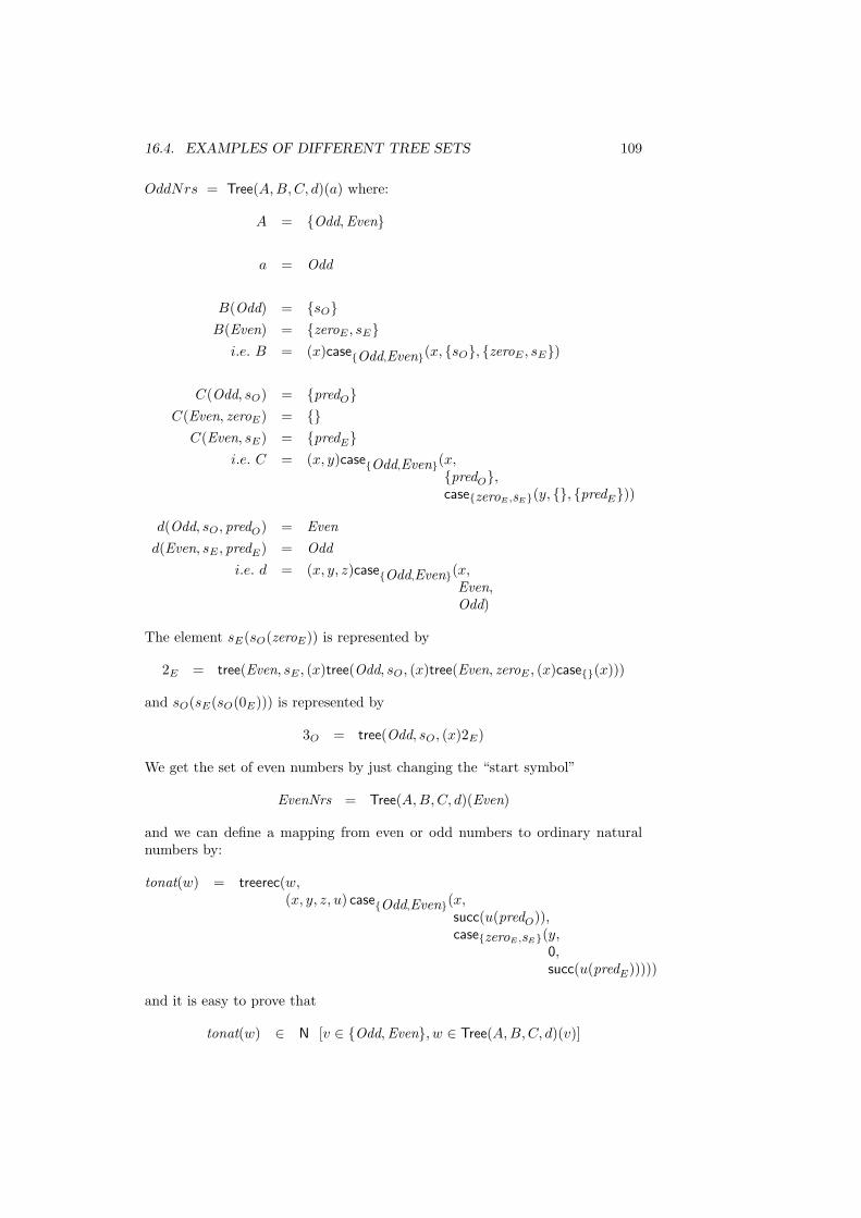
16.4. EXAMPLES OF DIFFERENT TREE SETS 109
OddNrs = Tree(A,B,C, d)(a) where:
A = {Odd,Even}
a = Odd
B(Odd) = {sO}B(Even) = {zeroE , sE}
i.e. B = (x)case{Odd,Even}(x, {sO}, {zeroE , sE})
C(Odd, sO) = {predO}C(Even, zeroE) = {}
C(Even, sE) = {predE}i.e. C = (x, y)case{Odd,Even}(x,
{predO},case{zeroE ,sE}(y, {}, {predE}))
d(Odd, sO, predO) = Evend(Even, sE , predE) = Odd
i.e. d = (x, y, z)case{Odd,Even}(x,Even,Odd)
The element sE(sO(zeroE)) is represented by
2E = tree(Even, sE , (x)tree(Odd, sO, (x)tree(Even, zeroE , (x)case{}(x)))
and sO(sE(sO(0E))) is represented by
3O = tree(Odd, sO, (x)2E)
We get the set of even numbers by just changing the “start symbol”
EvenNrs = Tree(A,B, C, d)(Even)
and we can define a mapping from even or odd numbers to ordinary naturalnumbers by:
tonat(w) = treerec(w,(x, y, z, u) case{Odd,Even}(x,
succ(u(predO)),case{zeroE ,sE}(y,
0,succ(u(predE)))))
and it is easy to prove that
tonat(w) ∈ N [v ∈ {Odd,Even}, w ∈ Tree(A,B,C, d)(v)]
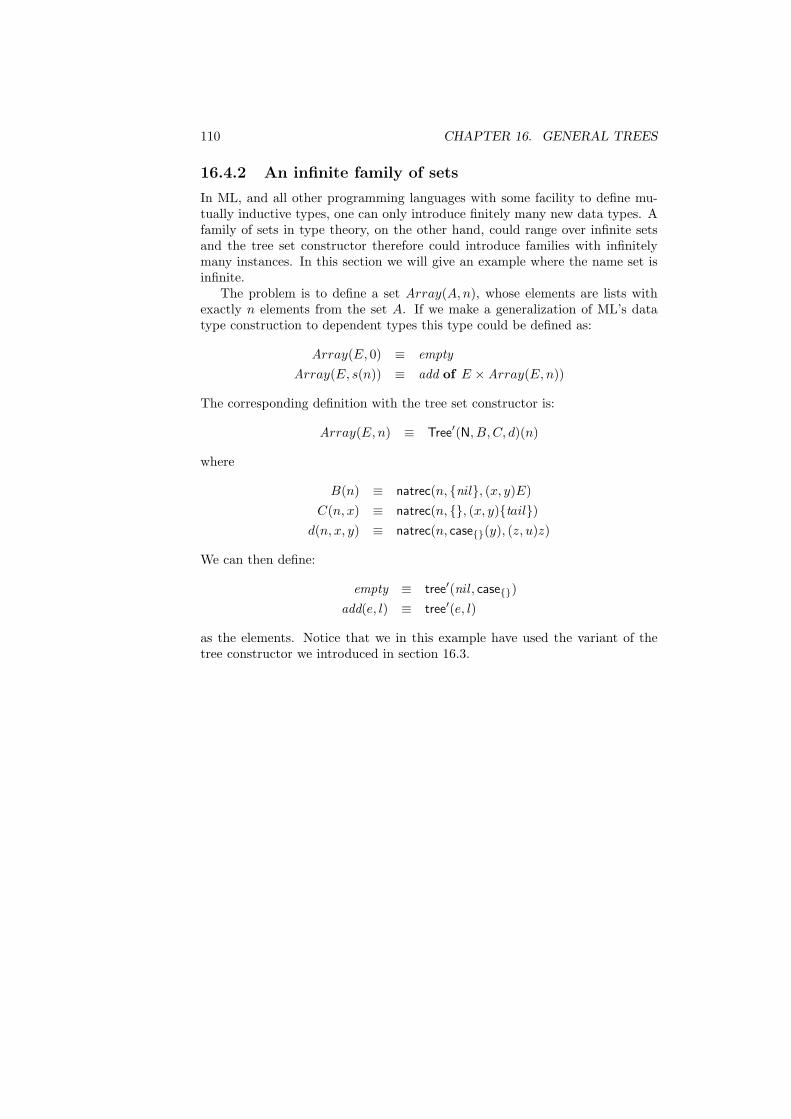
110 CHAPTER 16. GENERAL TREES
16.4.2 An infinite family of sets
In ML, and all other programming languages with some facility to define mu-tually inductive types, one can only introduce finitely many new data types. Afamily of sets in type theory, on the other hand, could range over infinite setsand the tree set constructor therefore could introduce families with infinitelymany instances. In this section we will give an example where the name set isinfinite.
The problem is to define a set Array(A,n), whose elements are lists withexactly n elements from the set A. If we make a generalization of ML’s datatype construction to dependent types this type could be defined as:
Array(E, 0) ≡ emptyArray(E, s(n)) ≡ add of E ×Array(E,n))
The corresponding definition with the tree set constructor is:
Array(E,n) ≡ Tree′(N, B, C, d)(n)
where
B(n) ≡ natrec(n, {nil}, (x, y)E)C(n, x) ≡ natrec(n, {}, (x, y){tail})
d(n, x, y) ≡ natrec(n, case{}(y), (z, u)z)
We can then define:
empty ≡ tree′(nil, case{})add(e, l) ≡ tree′(e, l)
as the elements. Notice that we in this example have used the variant of thetree constructor we introduced in section 16.3.

Part II
Subsets
111


Chapter 17
Subsets in the basic settheory
We will in this section add sets formed by comprehension directly to the basicset theory in a similar way as we have introduced the other primitive sets. Aswe already have mentioned, we will in this approach not be able to formulate asatisfactory elimination rule.
Let A be a set and B a propositional function (family of sets) defined onthe set A, i.e. assume A set and B(x) set [x ∈ A]. From these assumptionsand the explanation of what it means to be a set, it follows that the canonicalelements and their equality relation is understood for the set A and for the setB(a) whenever a ∈ A.
The subset of A with respect to B is denoted
{|}(A,B)
where {|} is a constant of arity 0⊗(0→→0)→→0. Instead of {|}(A,B), we shalluse the more lucid notation
{x∈A | B(x)}
This set forming operation is defined, as all the other sets, by prescribing howto form canonical elements and how to form equal canonical elements: if a is acanonical element in the set A and B(a) is true, i.e. if there exists an elementb ∈ B(a), then a is also a canonical element in the set {x∈A | B(x)}. And if aand c are equal canonical elements in the set A and B(a) is true, then a and c arealso equal canonical elements in the set {x∈A | B(x)}. Since every propositionalfunction is extensional in the sense that it yields equal propositions (sets) whenit is applied to equal elements, it follows from a = c ∈ A and B(x) set [x ∈ A]that B(a) and B(c) are equal propositions (sets). And, consequently, from therequirement that B(a) is true, we immediately get that also B(c) is true.
The introduction of the canonical elements makes sense precisely when A isa set and B(x) is a set under the assumption that x ∈ A. Hence, the formationrule for the subset becomes:
113

114 CHAPTER 17. SUBSETS IN THE BASIC SET THEORY
Subset – formation
A set B(x) set [x ∈ A]{x∈A | B(x)} set
For many sets, the prescription of how to form canonical elements and equalcanonical elements immediately justifies the introduction rules, since the re-quirements for forming canonical elements can be expressed as premises of theintroduction rules. The canonical elements of the subset, however, cannot jus-tify an introduction rule in this way, because the requirement that a should bea canonical element in A cannot be expressed as a premise. So we cannot formthe introduction rule according to the general scheme. Instead, the introductionrule introduces expressions both of canonical and noncanonical form. From theexplanation of the judgement a ∈ A, we know that a, when evaluated, will yielda canonical element in the set A as result. So if B(a) is true, we know that awill also yield a canonical element in the set {x∈A | B(x)}. The introductionrule becomes:
Subset – introduction 1
a ∈ A b ∈ B(a)a ∈ {x∈A | B(x)}
And similarly, if a1 = a2 ∈ A, the evaluation of a1 and a2 will yield equalcanonical elements in the set A as result and, therefore, if B(a1) is true, theywill yield equal canonical elements in the set {x∈A2 | B2(x)}. Since b ∈ B(a1)it follows from a1 = a2 ∈ A and b ∈ B(a1) that b ∈ B(a2). This justifies thesecond introduction rule for subsets:
Subset – introduction 2
a1 = a2 ∈ A b ∈ B(a1)a1 = a2 ∈ {x ∈ A | B(x)}
The subsets are different from all other sets in that the canonical and non-canonical forms of expressions depend only on the parameter set A. So from anelement expression alone, it is impossible to determine the form of its set; it maybelong to A as well as to a subset of A. But this cannot cause any confusion,since an element is always given together with its set.
An elimination rule which captures the way we have introduced elements ina subset is impossible to give in type theory because when we have an elementa in a subset {x ∈ A | B(x)} we have no explicit construction of the proofelement of B(a). The best formulation of an elimination rule we can give is thefollowing:

115
Subset – elimination 1
c ∈ {x ∈ A | B(x)} d(x) ∈ C(x) [x ∈ A, y ∈ B(x)]d(c) ∈ C(c)
where y must not occur free in d nor in C
Because of the syntactical restriction on free variables in the subset-eliminationrule the strength of this rule is connected with the possibility of having rules intype theory where free variables, other than those discharged by the rule, maydisappear in the conclusion. In our basic formulation of Martin-Lof’s set theorywith the intensional identity Id, there are very few possibilities to get rid of freevariables in an essential way.
The strength of adding subsets to set theory with the elimination rule aboveis discussed in detail in [90] where it is shown that propositions of the form
(∀x ∈ {z ∈ A | P (z)})P (x) (∗)
cannot in general be proved. In the intensional formulation we have of settheory, not even (∀x ∈ {z ∈ T | ⊥})⊥ can be derived. The proof in [90] of thisis rather complicated, using a normalization argument.
Propositions of the form (∗) are important when modularizing programderivations, using a top-down approach and decomposing the specification intosubproblems. When solving the subproblems we may want to use lemmas whichhave already been proved. The main idea of splitting up a problem into lemmasis, in program derivation as well as in mathematics, that our original problemcan be reduced to the lemmas; in particular, there should be no need to lookinto the proofs of the lemmas. If we have a lemma which talks about subsets wecertainly want (∗) to be provable since if a ∈ {x ∈ A | P (x)} we want to be ableto conclude P (a) without having to investigate the proof of a ∈ {x ∈ A | P (x)}.
In set theory with the extensional equality Eq, there are more cases for which(∗) can be proved. Let P (x) set [x ∈ A]. The predicate P (x) is called stable if
¬¬P (x) → P (x) [x ∈ A]
Using strong Eq-elimination together with the universe, it is proved in [90] that(∗) holds for all stable predicates, that is
(∀x∈A)(¬¬P (x) → P (x)) → (∀x ∈ {z ∈ A | P (z)})P (x)
holds in the extensional theory. Extending the basic extensional set theory withsubset is discussed in detail in Salvesen [92].
It is also shown in [90] that if we put P (x) equal to
(∃y∈N)T (x, x, y) ∨ ¬(∃y∈N)T (x, x, y)
where T is Kleene’s T -predicate, and put A equal to N, then (∗) cannot bederived in Martin-Lof’s set theory extended with the above rules for subsetsirrespectively of how we formulate the remaining rules; the only requirementsare that the axiom of choice, as formulated in [69, 70], can be proved and thata typable term can be computed by a Turing machine.
So the approach of this chapter to introduce subsets in the same way as theother sets and interpret proposition as sets results in a very weak eliminationrule which, at least in the intensional theory, will not work in practice.

116 CHAPTER 17. SUBSETS IN THE BASIC SET THEORY
Chapter 18
The subset theory
In order to get an elimination rule by which we, for instance, can derive P (a) truefrom a ∈ {x∈A | P (x)} we will now, following ideas of Martin-Lof, give a newmeaning of the judgement A set. We then also have to give new explanationsof the other forms of judgement. All judgements will be explained in terms ofour previous explanations for set theory. We will call this new theory the subsettheory and refer to the earlier set theory as the basic set theory or just set theory.
The crucial difference between the basic set theory and the subset theory isthat propositions will no longer be viewed as sets in the subset theory. However,the semantics of propositions in the subset theory will use propositions as setsin the basic set theory. So we must first extend our language by introducingprimitive constants for the logical constants: &, ∨ and ⊃ of arity 0⊗0→→0, ⊥of arity 0, ∀ and ∃ of arity 0⊗(0→→0)→→0. We also need a primitive constant ID
of arity 0⊗0⊗0→→0 for forming the proposition that two elements of a certainset are equal. Instead of ID(A, a, b) we will often write a =A b.
We will give detailed explanations of the judgements for a subset theorywithout universes. The intuition behind the semantics is that a set A in thesubset theory consists of those elements x in a base set A′ in the basic set theorysuch that A′′(x) holds, where A′′ is a propositional function on A′ in the basicset theory. The situation with universes is somewhat more complicated and willbe discussed later in the chapter.
18.1 Judgements without assumptions
As when we explained the meaning of the judgements of the basic set theory,we first explain the judgements not depending on any assumptions.
117

118 CHAPTER 18. THE SUBSET THEORY
18.1.1 What does it mean to be a set?
To know the judgementA set
in the subset theory is to have a pair (A′, A′′) where we know thatA′ is a set in the basic set theory and that A′′ is a propositionalfunction on A′ in the basic set theory.
So in order to know that A is a set in the subset theory we must have A′ andA′′ and know the judgements
• A′ set
• A′′(x) prop [x ∈ A′]
in the way we already have explained in the basic set theory. Note that thejudgement A′′(x) prop [x ∈ A′] in the basic set theory is just an abbreviationof the judgement A′′(x) set [x ∈ A′].
18.1.2 What does it mean for two sets to be equal?
Let A and B be sets in the subset theory. According to the explanation of whatit means to be a set in the subset theory, we then have sets A′ and B′ andpropositional functions A′′ and B′′ on A′ and B′, respectively. To know thejudgement that A and B are equal sets in the subset theory is explained in thefollowing way:
To know that A and B are equal sets
A = B
in the sense of the subset theory, is to know that A′ and B′ are equalsets in the basic set theory and that A′′(x) and B′′(x) are equivalentpropositions on A′ in the sense of the basic set theory.
So in order to know that A and B are equal, we must know the judgements
• A′ = B′
• A′′(x) ⇔ B′′(x) true [x ∈ A′]
as explained in the basic set theory. Since propositions are interpreted as setsin the basic theory, the judgement A′′(x) ⇔ B′′(x) true [x ∈ A′] means that wehave an element in (A′′(x) → B′′(x))× (B′′(x) → A′′(x)) under the assumptionx ∈ A′.
18.1.3 What does it mean to be an element in a set?
According to the explanation of the judgement A set in the subset theory, Aconsists of those elements x in A′ such that A′′(x) holds:
To know the judgementa ∈ A
where A is a set in the sense of the subset theory, we must knowthat a is an element in A′ and that A′′(a) is true.

18.2. HYPOTHETICAL JUDGEMENTS 119
So in order to know that a is an element in the set A we must know the judge-ments
• a ∈ A′
• A′′(a) true
as explained in the basic set theory. Note that A′′(a) true means that we havean element in the set A′′(a).
18.1.4 What does it mean for two elements to be equal ina set?
If a ∈ A and b ∈ A then the explanation of equality between a and b is thefollowing.
To know that a and b are equal elements in a set A
a = b ∈ A
in the sense of the subset theory is to know the judgement
a = b ∈ A′
in the basic set theory.
So that two elements are equal in a subset means that they must be equalelements in the base set of the subset.
18.1.5 What does it mean to be a proposition?
To know a proposition P in the subset theory is to know a proposi-tion P ? in the basic set theory.
Since P may contain quantifiers ranging over subsets, P ? will depend on theinterpretation of subsets. Since propositions are interpreted as sets in the basicset theory, P ? is nothing but a set in the basic theory.
18.1.6 What does it mean for a proposition to be true?
To know that the proposition P is true in the subset theory is toknow that P ? is true in set theory.
So a proposition P is true in the subset theory if we have an element in the setP ? in the basic set theory.
18.2 Hypothetical judgements
The explanation of a judgement depending on assumptions is done, as in thebasic set theory, by induction on the number of assumptions. Leaving out higherorder assumptions, a member Ck in an arbitrary context C1, . . . , Cn in the subsettheory is either of the form xk ∈ Ak(x1, . . . , xk−1) where Ak(x1, . . . , xk−1) is asubset in the context C1, . . . , Ck−1 or of the form P (x1, . . . , xk) true where
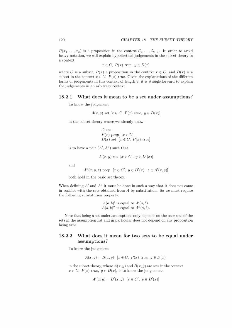
120 CHAPTER 18. THE SUBSET THEORY
P (x1, . . . , xk) is a proposition in the context C1, . . . , Ck−1. In order to avoidheavy notation, we will explain hypothetical judgements in the subset theory ina context
x ∈ C, P (x) true, y ∈ D(x)
where C is a subset, P (x) a proposition in the context x ∈ C, and D(x) is asubset in the context x ∈ C, P (x) true. Given the explanations of the differentforms of judgements in this context of length 3, it is straightforward to explainthe judgements in an arbitrary context.
18.2.1 What does it mean to be a set under assumptions?
To know the judgement
A(x, y) set [x ∈ C, P (x) true, y ∈ D(x)]
in the subset theory where we already know
C setP (x) prop [x ∈ C]D(x) set [x ∈ C, P (x) true]
is to have a pair (A′, A′′) such that
A′(x, y) set [x ∈ C ′, y ∈ D′(x)]
andA′′(x, y, z) prop [x ∈ C ′, y ∈ D′(x), z ∈ A′(x, y)]
both hold in the basic set theory.
When defining A′ and A′′ it must be done in such a way that it does not comein conflict with the sets obtained from A by substitution. So we must requirethe following substitution property:
A(a, b)′ is equal to A′(a, b).A(a, b)′′ is equal to A′′(a, b).
Note that being a set under assumptions only depends on the base sets of thesets in the assumption list and in particular does not depend on any propositionbeing true.
18.2.2 What does it mean for two sets to be equal underassumptions?
To know the judgement
A(x, y) = B(x, y) [x ∈ C, P (x) true, y ∈ D(x)]
in the subset theory, where A(x, y) and B(x, y) are sets in the contextx ∈ C, P (x) true, y ∈ D(x), is to know the judgements
A′(x, y) = B′(x, y) [x ∈ C ′, y ∈ D′(x)]

18.2. HYPOTHETICAL JUDGEMENTS 121
and
A′′(x, y) ⇔ B′′(x, y) true [x ∈ C ′, C ′′(x) true,P ?(x) true, y ∈ D′(x), D′′(x, y) true]
in the basic set theory.
So that the base sets of the two equal sets are equal only depends on the basesets of the subsets in the assumption list. The equivalence of the propositionalparts of the sets, however, may depend also on the propositional parts of thesets in the assumption list as well as on the truth of propositions.
18.2.3 What does it mean to be an element in a set underassumptions?
To know the judgement
a(x, y) ∈ A(x, y) [x ∈ C, P (x) true, y ∈ D(x)]
in the subset theory, where A(x, y) is a set in the context x ∈C, P (x) true, y ∈ D(x), is to know the judgements
a(x, y) ∈ A′(x, y) [x ∈ C ′, y ∈ D′(x)]
and
A′′(x, y, a(x, y)) true [x ∈ C ′, C ′′(x) true,P ?(x) true, y ∈ D′(x), D′′(x, y) true]
in the basic set theory.
Note that a(x, y) is an element in the base set of A(x, y) only depends on thebase sets of the sets in the assumption list and in particular does not dependon any proposition being true.
18.2.4 What does it mean for two elements to be equal ina set under assumptions?
To know the judgement
a(x, y) = b(x, y) ∈ A(x, y) [x ∈ C, P (x) true, y ∈ D(x)]
in the subset theory, where a(x, y) ∈ A(x, y) and b(x, y) ∈ A(x, y) inthe context x ∈ C, P (x) true, y ∈ D(x), is to know the judgement
a(x, y) = b(x, y) ∈ A′(x, y) [x ∈ A′, y ∈ B′(x)]
in the basic set theory.
So that two elements are equal in a set under assumptions means that theymust be equal already as elements in the base set, only depending on the basesets of the sets in the assumption list.

122 CHAPTER 18. THE SUBSET THEORY
18.2.5 What does it mean to be a proposition under as-sumptions?
To know the judgement
Q(x, y) prop [x ∈ C, P (x) true, y ∈ D(x)]
in the subset theory is to know the judgement
Q?(x, y) prop [x ∈ C ′, y ∈ D′(x)]
in the basic set theory.
We must also require the substitution property
Q(a, b)? is equal to Q?(a, b)
18.2.6 What does it mean for a proposition to be trueunder assumptions?
To know the judgement
Q(x, y) true [x ∈ C, P (x) true, y ∈ D(x)]
in the subset theory, where Q(x, y) is a proposition in the contextx ∈ C, P (x) true, y ∈ D(x), is to know the judgement
Q?(x, y) true [x ∈ C ′, C ′′(x) true,P ?(x) true, y ∈ D′(x), D′′(x, y) true]
in the basic set theory.
18.3 General rules in the subset theory
With the exception of the rule Proposition as set, all the general rules of thebasic set theory also hold in the subset theory. Let us as an example justify theSet equality rule
a ∈ A A = B
a ∈ B
By the explanations of judgements of the form a ∈ A and A = B in the subsettheory, we have to show that if the judgements a ∈ A′, A′′(a) true, A′ = B′ andA′′(x) ⇔ B′′(x) true [x ∈ A′] all hold in set theory, then a ∈ B′ and B′′(a) truealso hold in set theory. That a ∈ B′ holds follows from a ∈ A′, A′ = B′ and theType equality rule in set theory. From A′′(a) true and A′′(x) → B′′(x) true [x ∈A′] we get that B′′(a) is true by substitution and →-elimination.
Since a proposition is interpreted as a set in the basic set theory, we did notintroduce judgements of the forms P prop and P true in the formalization ofset theory. For instance, an assumption of the form P true in set theory can beunderstood as an assumption y ∈ P where y is a new variable. In the subsettheory, however, we must have judgements of the forms P prop and P true inthe formal system and therefore we have to add general rules involving thesetwo forms of judgement.

18.3. GENERAL RULES IN THE SUBSET THEORY 123
AssumptionP prop
P true [P true]
By the explanation of what it means to be a proposition in the subset theory,we know that P ? is a proposition, that is a set, in the basic set theory. Hence,by the assumption rule in set theory, we have y ∈ P ? [y ∈ P ?] which is themeaning of P true [P true].
The judgementC(x) prop [x ∈ A]
means that the judgement C?(x) set [x ∈ A′] holds in the basic set theory. Bythe rule Substitution in sets and the substitution property of C?(x) we thereforehave the rule
Substitution in propositions
C(x) prop [x ∈ A] a ∈ A
C(a) prop
The ruleCut rule for propositions
Q prop [P true] P true
Q prop
is justified in the following way. The judgement Q prop [P true] in the subsettheory means that Q? set [y ∈ P ?] in set theory and the judgement P truemeans that we have an element a in the set P ?. By Substitution in sets wetherefore get Q? set, that is, Q? prop as desired.
In a similar way, we can justify the rulesCut rule for equal sets
A = B [P true] P true
A = B
Cut rule for true propositions
Q true [P true] P true
Q true
Cut rule for elements in sets
a ∈ A [P true] P true
a ∈ A
Cut rule for equal elements in sets
a = b ∈ A [P true] P true
a = b ∈ A

124 CHAPTER 18. THE SUBSET THEORY
18.4 The propositional constants in the subsettheory
Without a universe of propositions, which we will introduce later, the proposi-tional constants are the logical constants and the propositional equality.
18.4.1 The logical constants
Let P and Q be propositions in the subset theory. This means that we havepropositions, that is sets, P ? and Q? in the basic theory. Propositions built upfrom P and Q by the sentential connectives are given meaning in the followingway:
(P&Q)? is defined to be the proposition P ? ×Q?.
(P ∨Q)? is defined to be the proposition P ? + Q?.
(P ⊃Q)? is defined to be the proposition P ? → Q?.
The truth T and absurdity ⊥ are given meaning in a similar way:
T? is defined to be the proposition T.
⊥? is defined to be the proposition ∅.
So a sentential constant is given meaning by the use of the same set formingconstant as when interpreting proposition as sets. However, the situation ismore complicated when we come to the quantifiers.
Let A be a set and P a propositional function on A in the subset theory. Wethen have, according to the meaning of being a set and a propositional functionon a set, a base set A′ and propositional functions A′′ and P ? defined on A′ inthe basic set theory. The propositions obtained from P by quantification on Aare given meaning in the following way:
The proposition ((∀x∈A)P (x))? is defined to be
(Πx∈A′)(A′′(x) → P ?(x))
The proposition ((∃x∈A)P (x))? is defined to be
(Σx∈A′)(A′′(x)× P ?(x))
It is now easy to justify the rules of first order logic as we have formulatedthem earlier. As an example, we justify the rules for the universal quantifier.
∀ – formation
A prop P (x) prop [x ∈ A](∀x∈A)P (x) prop
We must show that (Πx∈A′)(A′′(x) → P ?(x)) is a proposition, that is a set, inthe basic set theory from the assumptions that we already know the judgementsA′ set, A′′(x) prop [x ∈ A′] and P ?(x) prop [x ∈ A′]. By →-formation we

18.4. THE PROPOSITIONAL CONSTANTS IN THE SUBSET THEORY125
get A′′(x) → P ?(x) set [x ∈ A′] which gives (Πx∈A′)(A′′(x) → P ?(x)) set asdesired.
∀ – introductionP (x) true [x ∈ A](∀x∈A)P (x) true
That we know the judgement P (x) true [x ∈ A] in the subset theory meansthat we know the judgement P ?(x) true [x ∈ A′, A′′(x) true] in the basic settheory. So we have an expression b for which we know the judgement b(x) ∈P ?(x) [x ∈ A′, y ∈ A′′(x)] in the basic set theory. By →-introduction, we getλy.b(x) ∈ A′′(x) → P ?(x) [x ∈ A′] which, by Π-introduction, gives λx.λy.b(x) ∈(Πx∈A′)(A′′(x) → P ?(x)). Hence, we know the judgement (Πx∈A′)(A′′(x) →P ?(x)) true as desired.
∀ – elimination 1
(∀x∈A)P (x) true a ∈ A
P (a) true
Assume that we have expressions b and c for which we know the judgementsb ∈ (Πx∈A′)(A′′(x) → P ?(x)), a ∈ A and c ∈ A′′(a) in the basic set theory. ByΠ-elimination we get apply(b, a) ∈ A′′(a) → P ?(a) and then, by →-elimination,apply(apply(b, a), c) ∈ P ?(a). So P ?(a) is true in set theory as desired.
18.4.2 The propositional equality
Let A be a subset and a and b elements in A. Then the meaning of a =A b isgiven by
The proposition (a =A b)? is defined to be Id(A′, a, b).
We have the following rules for the propositional equality:= – formation
a ∈ A b ∈ A
a =A b prop
= – introductiona = b ∈ A
a =A b true
= – elimination
C(x) prop [x ∈ A] a =A b true C(a) true
C(b) true
We justify the elimination rule. The judgement a =A b true means that wehave an element c in the set Id(A′, a, b) and the judgement C(a) true means thatwe have an element d in the set C?(a) . Using Id-elimination on c ∈ Id(A′, a, b)and λu.u ∈ C∗(x) → C∗(x) [x ∈ A] we get idpeel(c, (x)λu.u) ∈ C∗(a) → C∗(b).Since d ∈ C∗(a) we then obtain, by →-elimination,
apply(idpeel(c, (x)λu.u), d) ∈ C∗(b)
So, C∗(b) is true in the basic set theory which is the meaning of the judgementC(b) true in the subset theory.

126 CHAPTER 18. THE SUBSET THEORY
18.5 Subsets formed by comprehension
Sets in the subset theory are built up by the set forming operations we alreadyhave in the basic set theory and by set comprehension. The semantics of subsetsintroduced by comprehension is the following:
{x ∈ A | P (x)}′ is defined to be the set A′ and {x ∈ A | P (x)}′′ isdefined to be the propositional function (z)(A′′(z)× P ?(z)) on A′.
The formation ruleSubset – formation
A set P (x) prop [x ∈ A]{x ∈ A | P (x)} set
is justified in the following way. We assume that we know the interpretations ofthe premises, that is that we know the judgements A′ set, A′′(x) prop [x ∈ A′]and P ?(x) prop [x ∈ A′] as explained in the basic set theory. Since {x ∈A | P (x)}′ is defined to be A′, we get that {x ∈ A | P (x)}′ is a set. By ×-introduction we get that A′′(x)× P ?(x) is a proposition when x ∈ A′.
It is also easy to justify the introduction rule:Subset – introduction
a ∈ A P (a) true
a ∈ {x ∈ A | P (x)}
Now we obtain the desired elimination rules for comprehension.Subset – elimination for sets
a ∈ {x ∈ A | P (x)} c(x) ∈ C(x) [x ∈ A, P (x) true]c(a) ∈ C(a)
This rule is justified as follows. We assume that we already know the judgements
a ∈ A′
A′′(a)× P ?(a) truec(x) ∈ C ′(x) [x ∈ A′]C ′′(c(x)) true [x ∈ A′, A′′(x) true, P ?(x) true]
in the basic set theory. From the first and third of these judgements we get, bysubstitution and the substitution property, that c(a) ∈ C(a)′. By ×-elimination,substitution and the substitution property we get from the first, second andfourth judgements that C(a)′′(c(a)) true holds. In a similar way we can justifythe rule
Subset – elimination for propositions
a ∈ {x ∈ A | P (x)} Q(x) true [x ∈ A, P (x) true]Q(a) true
By putting Q(x) equal to P (x) in Subset-elimination for proposition we seethat now we can derive P (a) true from a ∈ {x ∈ A | P (x)} which in general isnot possible in the basic theory.

18.6. THE INDIVIDUAL SET FORMERS IN THE SUBSET THEORY 127
18.6 The individual set formers in the subsettheory
For each set A obtained by any of the individual set formers we have to definethe set A′ and the propositional function A′′ on A′ in the basic set theory. Ingeneral, the formation of a set is made in a context which we will not mentionexplicitly. In particular, the substitution property must be satisfied when wesubstitute terms for the variables in the context. Because of the inductive waythe set is introduced, it is easy to see that the substitution property holds.
To the rules for the individual sets in the basic theory, we will add rules forproving the truth of propositions by structural induction. These new rules willbe called elimination rules for propositions. For the inductively defined sets wewill also give equality rules which will reflect their interpretation in the basicset theory.
18.6.1 Enumeration sets
An enumeration set has the same elements in the subset theory as it has in thebasic theory:
{i1, . . . , in}′ is defined to be the set {i1, . . . , in} and {i1, . . . , in}′′ isdefined to be the propositional function (z)T on {i1, . . . , in}.
To the rules for enumeration sets in the basic theory we have to add the rule{i1, . . . , in} – elimination for propositions
a ∈ {i1, . . . , in}Q(x) prop [x ∈ {i1, . . . , in}]Q(i1) true
...Q(in) true
Q(a) true
This rule is justified in the following way. That the judgement Q(x) prop [x ∈{i1, . . . , in}] holds in the subset theory means that Q?(x) set [x ∈ {i1, . . . , in}]holds in the basic theory since {i1, . . . , in}′ is {i1, . . . , in}. The judgementQ(ik) true means that we have an element bk in the set Q∗(ik). Hence, we canuse {i1, . . . , in}-elimination 1 to obtain case(a, b1, . . . , bn) ∈ Q∗(a). So Q∗(a)is true in the basic set theory and, hence, Q(a) is true in the subset theory asdesired.
The other rules for enumeration sets are also straightforward to justify.
18.6.2 Equality sets
The main purpose of the equality sets in the basic set theory is to reflect thejudgemental equality to the propositional level. Since propositions are not inter-preted as sets in the subset theory, we have introduced equality as a primitiveproposition, so there is really no need of equality sets in the subset theory.However, they can be given semantics in the subset theory:
Id(A, a, b)′ is defined to be the set Id(A′, a, b) and Id(A, a, b)′′ is de-fined to be the propositional function (z)T on Id(A′, a, b).

128 CHAPTER 18. THE SUBSET THEORY
18.6.3 Natural numbers
The natural numbers in the subset theory are, of course, the same as the naturalnumbers in the basic set theory:
N′ is defined to be the set N and N′′ is defined to be the propositionalfunction (z)T′′ on N.
The rules for N are all easy to justify and as an example we justify the newN-elimination rule.
N – elimination for propositions
Q(x) prop [x ∈ N]a ∈ NQ(0) trueQ(succ(x)) true [x ∈ N, Q(x) true]Q(a) true
For the justification of the rule, assume that we have expressions d and e andknow the judgements a ∈ N, d ∈ Q?(0) and e(x, y) ∈ Q?(succ(x)) [x ∈ N, y ∈Q?(x)] as explained in the basic set theory. By the N-elimination rule in thebasic set theory, we get natrec(a, d, e) ∈ Q?(a). So Q(a) is true in the subsettheory as desired.
18.6.4 Cartesian product of a family of sets
An element f in a cartesian product of a family B of sets on a set A in thesubset theory is an element in the cartesian product (Πx∈A′)B′(x) in the basictheory, such that when it is applied on an element a in A′ such that A′′(a) istrue, it gives an element in B′(a) such that B′′(a, apply(f, a)) is true:
((Πx∈A)B(x))′ is defined to be the set (Πx∈A′)B(x)′ and((Πx∈A)B(x))′′ is defined to be the propositional function
(z)((Πx∈A′)(A′′(x) → B(x)′′(apply(z, x))))
on the set (Πx∈A′)B(x)′.
The rule we have to add isΠ – elimination for propositions
f ∈ (Πx∈A)B(x) Q(λ(y)) true [y(x) ∈ B(x) [x ∈ A]]Q(f) true
In this rule we must use a higher order assumption, which we have not discussedfor the subset theory. But we leave out the details of extending our semantics tojudgements depending on higher order assumption. Note that the eliminationrule for Π involving apply cannot be used to obtain an induction principle forpropositions over a Π-type.
We can also justify the equality rule

18.6. THE INDIVIDUAL SET FORMERS IN THE SUBSET THEORY 129
Π-subset – equality
A setB(x) set [x ∈ A]P (x) prop [x ∈ A]Q(x, y) prop [x ∈ A, y ∈ B(x)](Πx∈{u ∈ A | P (u)}){v ∈ B(x) | Q(x, v)} ={z ∈ (Πx∈A)B(x) | (∀u∈A)(P (u)⊃Q(u, apply(z, x)))}

130 CHAPTER 18. THE SUBSET THEORY
18.6.5 Disjoint union of two sets
The semantics of a disjoint union of two sets is the following:
(A + B)′ is defined to be the set A′ + B′ and (A + B)′′ is defined tobe the propositional function
(z)((∃x∈A′)(A′′(x) × Id(A′, z, inl(x))) +(∃y∈B′)(B′′(y) × Id(B′, z, inr(y))))
on the set A′ + B′.
The elimination rule we have to add is+ – elimination for propositions
c ∈ A + B Q(inl(x)) true [x ∈ A] Q(inr(y)) true [y ∈ B]Q(c) true
We also have the equality rule+-subset – equality
A set P (x) prop [x ∈ A] Q(y) prop [y ∈ B]{x ∈ A | P (x)} + {y ∈ B | Q(y)} ={z ∈ A + B |(∃x∈A)(P (x) & z =A inl(x)) ∨(∃y∈B)(Q(y) & z =B inr(y))}
18.6.6 Disjoint union of a family of sets
The semantics of a disjoint union of a family of sets is given by:
((Σx∈A)B(x))′ is defined to be (Σx∈A′)B′(x) and((Σx∈A)B(x))′′ is defined to be the propositional function
(z)(A′′(fst(z))×B(fst(z))′′(snd(z)))
on (Σx∈A′)B′(x).
We have to add the ruleΣ – elimination for propositions
c ∈ Σ(A,B) Q(〈x, y〉) true [x ∈ A, y ∈ B(x)]Q(c) true
We can also justify the equality ruleΣ-subset – equality
A setB(x) set [x ∈ A]P (x) prop [x ∈ A]Q(x, y) prop [x ∈ A, y ∈ B(x)](Σx∈{u ∈ A | P (u)}){v ∈ B(x) | Q(x, v)} ={z ∈ (Σx∈A)B(x) | P (fst(z))×Q(fst(z), snd(z))}

18.7. SUBSETS WITH A UNIVERSE 131
18.6.7 Lists
Let A be a set in the subset theory. The base set List(A)′ is then put equal tothe set List(A′) in the basic set theory. The propositional function List(A)′′ onList(A′) must satisfy that List(A)′′(nil) is true and, for a ∈ A′ and b ∈ List(A′),that List(A)′′(cons(a, b)) is true if A′′(a) and List(A)′′(b) both are true. SoList(A)′′ must be defined by a set valued recursion. The only way we can dothis is by using the universe U and we then obtain the following semantics forList(A):
List(A)′ is defined to be the set List(A′) and List(A′′) is defined tobe the propositional function
(z)(Set(listrec(z, T, (x, y, u)(A′′(x) × u))))
By the notation C we mean the code for the small set C. The code C can bedefined by induction on the formation of the set C.
The use of U when giving semantics to List(A) is not satisfactory since itcannot be extended to subsets involving a universe for subsets. We will discussthis problem in the section on the universe in the subset theory and suggestother ways of giving semantics to List(A).
18.6.8 Well-orderings
As for lists, we must use the universe when giving semantics for well-orderings:
((Wx∈A)B(x))′ is defined to be the set (Wx∈A′)B′(x) and ((Wx∈A)B(x))′′ is defined to be the propositional function
(z)(Set(wrec(z, (x, y, u)(A′′(x) × (Πv∈B(x)′)(B(x)′′(v)→u(v))))))
18.7 Subsets with a universe
We will now introduce a subset U reflecting the subsets introduced so far and asubset P reflecting the propositions we have introduced. We must then extendthe syntax by adding constants
&, ∨, ⊃ , ⊥ ∃, ∀ and ID
which code the propositional constants and a constant Prop for the functionwhich decodes an element in P.
We first give the rules and then indicate how an interpretation of the subsettheory extended with U and P can be given in the basic set theory, using theuniverse U of the basic set theory.
P – formationP prop
P – introduction 1
P ∈ P Q ∈ P
P &Q ∈ P

132 CHAPTER 18. THE SUBSET THEORY
Prop – introduction 1
P ∈ P Q ∈ P
Prop(P &Q) ⇔ (Prop(P )&Prop(Q))
P – introduction 2
P ∈ P Q ∈ P
P ∨Q ∈ P
Prop – introduction 2
P ∈ P Q ∈ P
Prop(P ∨Q) ⇔ (Prop(P ) ∨ Prop(Q))
P – introduction 3
P ∈ P Q ∈ P
P ⊃Q ∈ P
Prop – introduction 3
P ∈ P Q ∈ P
Prop(P ⊃Q) ⇔ (Prop(P )⊃Prop(Q))
P – introduction 4
⊥ ∈ P
Prop – introduction 4
Prop(⊥) ⇔ ⊥
P – introduction 5
A ∈ U P (x) ∈ P [x ∈ Set(A)]∀(A,P ) ∈ P
Prop – introduction 5
A ∈ U P (x) ∈ P [x ∈ Set(A)]Prop(∀(A,P )) ⇔ (∀x∈Set(A))Prop(P (x))
P – introduction 6
A ∈ U P (x) ∈ P [x ∈ Set(A)]∃(A,P ) ∈ P
Prop – introduction 6
A ∈ U P (x) ∈ P [x ∈ Set(A)]Prop(∃(A,P )) ⇔ (∃x∈Set(A))Prop(P (x))

18.7. SUBSETS WITH A UNIVERSE 133
P – introduction 7
A ∈ U a ∈ Set(A) b ∈ Set(A)ID(A, a, b) ∈ P
Prop – introduction 7
A ∈ U a ∈ Set(A) b ∈ Set(A)ID(A, a, b) ⇔ ID(A, a, b)
To the rules for U in the basic set theory, excluding the elimination rule, wemust add rules reflecting subsets introduced by comprehension.
U – introduction 9
A ∈ U P (x) ∈ P [x ∈ Set(A)]
{|}(A,P ) ∈ U
Set – introduction 9
A ∈ U P (x) ∈ P [x ∈ Set(A)]
Set({|}(A,P )) = {x ∈ Set(A) | Prop(P (x))}
We will now indicate how the subset theory with U and P can be interpretedin the basic set theory. The interpretation of U will then reflect the interpreta-tion we already have given of the subset theory without a universe. This leadsto the following definition of U′:
U′ ≡ (Σx′∈U)(Set(x′) → U)
where U in the definiens is the universe in the basic set theory. U′′ is triviallydefined by
U′′ ≡ (z)T
In the interpretation of the subset theory without a universe, the elements ofa set are interpreted by themselves. However, this is no longer possible whenhaving a universe since an element in U′ is a pair, reflecting that a set A in thesubset theory is interpreted as a set A′ in the basic set theory together witha propositional function A′′ on A′. So if a ∈ U in the subset theory, then wecannot have a ∈ U′; instead we must also interpret a as a pair, which we willdenote by a′.
The interpretation of Set is then given by
Set(a)′ ≡ Set(fst(a′))Set(a)′′(z) ≡ Set(apply(snd(a′), z))
Since propositions are interpreted as sets, the interpretation of P must reflectthis:
P′ ≡ U
P′′(z) ≡ T

134 CHAPTER 18. THE SUBSET THEORY
The interpretation of Prop is then given by
Prop(a)′ ≡ Set(a′)Prop(a)′′(z) ≡ T
We must now also define the mapping ′ on elements. For codes of sets formedby comprehension, we have
{|}(a, b)′ ≡ 〈fst(a′), λz.(apply(snd(a′), z)&b′(z)〉
The mapping ′ is defined in a similar way for elements coding sets of the otherforms, reflecting the interpretation of the corresponding set. The mapping ′ willcommute with all the constants for elements which are not codes in U. So, forinstance, pair(a, b)′ ≡ pair(a′, b′).
When defining ′ on codes for lists and well-orderings there is, however, aproblem since the interpretation of these types is using the universe. One wayof solving this problem would be to add an infinite sequence
U1, . . . ,Un, . . .
of universes so that when interpreting Un one could use Un+1. Another way,discussed in [102], would be to extend the basic set theory with the possibilityof defining sets directly by recursion, not using the universe. Defining sets byinduction on lists, we would have to extend the syntax with a new constantListrec of arity 0⊗0⊗(0⊗0⊗0→→0)→→0 and add the rules
Listrec – formation
l ∈ List(A)C setE(x, y, Z) set [x ∈ A, y ∈ List(A), Z set]
Listrec(l, C, E) set
Listrec – equality 1
C set E(x, y, Z) set [x ∈ A, y ∈ List(A), Z set]Listrec(nil, C, E) = C
Listrec – equality 2
l ∈ List(A)C setE(x, y, Z) set [x ∈ A, y ∈ List(A), Z set]Listrec(a.l, C, E) = E(a, l, Listrec(l, C, E))
We can now give the semantics for lists in the subset theory without usinga universe:
List(A)′ is defined to be the set List(A′) and List(A)′′ is defined to bethe propositional function (z)((Listrec(z,T, (x, y, Z)(A′′(x) × Z))))

Part III
Monomorphic sets
135


Chapter 19
Types
In the previous chapters, we have defined a collection of sets and set formingoperations and presented proof rules for these sets. We have introduced theconstants for each set and then presented the proof rules in a natural deductionstyle. Another way of introducing sets is to use the more primitive notion oftype. Intuitively, a type is a collection of objects together with an equivalencerelation. Examples of types are the type of sets, the type of elements in a set,the type of propositions, the type of set-valued functions over a given set, andthe type of predicates over a given set.
In this chapter we will describe a theory of types and show how it can beused to present a theory of sets. We will get possibilities of using variablesranging over sets and higher order objects. The possibility of abstracting overthese kind of variables is essential for structuring big programs and proofs. Italso gives possibilities to use more elegant formulations of the elimination rulesfor the Π-set and the well-orderings. The theory of types can also be used asa logical framework [48] in which it is possible to formalize different logics. Itcan also be used as a theory of expressions where the types replaces the arities;hence, we will in this chapter not rely on the theory of expressions developed inchapter 3.
If one looks in a text book on logic like, for instance, Kleene’s Introductionto Metamathematics, one hardly finds any completely formal derivations. Ingeneral, the derivations depend on metavariables ranging over formulas. Forinstance, in the formal derivation
x = y &x = z
x = y
x = y &x = z⊃x = y
we can replace the formulas x = y and x = z by arbitrary formulas A and Brespectively thereby obtaining the schematic derivation
A &B
A
(A &B)⊃A
which no longer is a formal derivation in predicate logic.
137

138 CHAPTER 19. TYPES
Most of the derivations in this book are also made under some general as-sumptions like “Let A be a set and B(x) a family of sets over A”. Whenimplementing type theory on a computer these kinds of assumptions have tobe made formal. In the Nuprl-system [25] this is made by using universes; forinstance the assumption
“Let X be a set”
is translated into the formal assumption
X ∈ U
However, this does not really capture the assumption that X is an arbitrary set,because U is only the set of small sets which has a fixed inductive definition.What we really want to assume is that X is an arbitrary set, that is, somethingsatisfying the semantical requirements of being a set. In particular, X may inthe future be interpreted as some set which we have not yet defined. It mayalso be interpreted as some set involving U and then it cannot be a small set.
19.1 Types and objects
We will now extend type theory so that assumptions like “X is a set” can bemade. We will do that by introducing an even more basic concept than that ofa set, namely the notion of type. Intuitively, a type is a collection of objectstogether with an equivalence relation.
What does it mean that something is a type? To know that A is a type is toknow what it means to be an object of the type, as well as what it means for twoobjects to be the same. The identity between objects must be an equivalencerelation and it must be decidable. The requirement of decidability of identitycomes from the general requirement of decidability of the new forms of judge-ments that we are introducing in this chapter. In these judgements everythingis there which is needed to be convinced of them: They carry their own proof.
As an example of a type, we will later define the type Set whose objects aremonomorphic sets by explaining what it means to be a set as well as what itmeans for two sets to be the same.
We will writeA type
for the judgement that A is a type. That a is an object of type A is written
a : A
and that a and b are the same object of type A will be written
a = b : A
and, finally, that two types A and B are identical will be written
A = B
What does it mean for two types to be the same? Two types are the sameif an object of one type is also an object of the other type and identical objectsof the one type are identical objects of the other type.

19.2. THE TYPES OF SETS AND ELEMENTS 139
19.2 The types of sets and elements
The type Set which contains (monomorphic) sets as objects is explained byexplaining what a set is and when two sets are identical. To know a set A isto know how the canonical elements of A are formed and when two canonicalelements are identical. Two sets are identical if a canonical element of one setis a canonical element of the other set and if two identical canonical elementsin one set also are identical in the other set.
Hence, we have the axiomSet formation
Set type
Notice that this explanation of what the type Set is, is totally open. Wehave not exhausted the possibilities of defining new sets. This is in contrastwith the set U, whose canonical elements are codings of a fixed number of setconstructing operations. A set is always an inductive structure, we know thata canonical element in it has been formed according to one of its introductionrules.
If A is a set, then El(A) is a type. It is the type whose objects are theelements of A. We know that a is an object in El(A) if we know that the valueof a is a canonical element of A. Two objects in El(A) are identical if theirvalues are identical canonical elements in A. So we have the rules
El-formation
A : Set
El(A) type
A = B : Set
El(A) = El(B)
We will use the abbreviations
A set ≡ A : Set
a ∈ A ≡ a : El(A)
in accordance with the earlier used notation.
19.3 Families of types
In much the same way as the notion of set is extended to families of sets, wewill now introduce families of types.
A context is a sequence
x1 : A1, x2 : A2, . . . , xn : An
such that
• A1 is a type,
• A2[x1 := a1] is a type for an arbitrary object a1 of type A1,...

140 CHAPTER 19. TYPES
• An[x1 := a1][x2 := a2] · · · [xn−1 := an−1] is a type for arbitrary objectsa1, a2, . . . , an−1 of types
A1, A2[x1 := a1], . . . , An−1[x1 := a1][x2 := a2] · · · [xn−2 := an−2]
respectively.
That A is a family of types in the context
x1 : A1, x2 : A2, . . . , xn : An,
which we formally write
A type [x1 : A1, x2 : A2, . . . , xn : An]
means that
A[x1 := a1][x2 := a2] · · · [xn := an] is a type for arbitrary objectsa1, a2, . . . , an−1 of types A1, A2[x1 := a1], . . . ,An[x1 := a1][x2 := a2] · · · [xn−1 := an−1] respectively.
As for families of sets, we also require that A must be extensional in the context,that is, if
a1 = b1 : A1,a2 = b2 : A2[x1 := a1],
...an = bn : An[x1 := a1][x2 := a2] · · · [xn−1 := an−1]
then it follows from
A type [x1 : A1, . . . , xn : An]
that
A[x1 := a1][x2 := a2] · · · [xn := an] = A[x1 := b1][x2 := b2] · · · [xn := bn]
As an example, the two rules for El-formation express that El(X) is a familyof types over Set.
The explanation of the remaining three forms of judgements:
A = Ba : A
a = b : A
in the contextx1 : A1, x2 : A2, . . . , xn : An
is done in a similar way as the first form
A type [x1 : A1, x2 : A2, . . . , xn : An]
by reducing the explanation to the corresponding form with empty context bysubstituting appropriate closed expressions for the variables.

19.4. GENERAL RULES 141
19.4 General rules
Since the identity relation on a type is required to be an equivalence relationand since two types are identical if they have the same objects and identicalobjects of one of the types are also identical objects of the other, we have thefollowing identity rules.
Reflexivity
a : A
a = a : A
A type
A = A
Symmetry
a = b : A
b = a : A
A = B
B = A
Transitivity
a = b : A b = c : A
a = c : A
A = B B = C
A = C
Type identity
a : A A = B
a : B
a = b : A A = B
a = b : B
The explanations of families of types in a context of the form x : A directlygive rules for substitution:
Substitution in types
C type [x : A] a : A
C[x := a] type
C type [x : A] a = b : A
C[x := a] = C[x := b]
Substitution in objects
c : C [x : A] a : A
c[x := a] : C[x := a]c : C [x : A] a = b : A
c[x := a] = c[x := b] : C[x := a]
Substitution in identical types
B = C [x : A] a : A
B[x := a] = C[x := a]
Substitution in identical objects
b = c : B [x : A] a : A
b[x := a] = c[x := a] : B[x := a]
These rules can in the same way as in chapter 5 be extended to generalcontexts of the form x1 : A1, x2 : A2, . . . , xn : An where n simultaneoussubstitutions are made.

142 CHAPTER 19. TYPES
19.5 Assumptions
Our main reason for introducing types is that we want the possibility to makeassumptions of a more general form than x ∈ A, where A is a set. The assump-tions we can now make are of the form
x : C
where C is a type. To be more formal, we have the ruleAssumption
C type
x : C [x : C]
The premise C type in this rule may depend on a nonempty context, but asusual in natural deduction, we only explicitly show that part of the contextwhich is changed by the rule. By using the axiom that Set is a type we can nowmake the assumption that X is an arbitrary set:
Set type
X : Set [X : Set]
which, by the definition above, we can also write
Set type
X set [X set]
Assumptions in set theory without types are always of the form
x ∈ A
where A is a set and they can now be obtained as special cases of assumptionsin the theory of types by the following derivation:
A set
El(A) type
x : El(A) [x : El(A)]
Using our notational conventions, we can write the conclusion of this derivation
x ∈ A [x ∈ A]
Note that this derivation is not formal because of the occurrence of the metavari-able A, which denotes an arbitrary set. It is now possible to make the derivationcompletely formal by making an assumption of the form X set:
Set type
X : Set [X : Set]El(X) type [X : Set]
x : El(X) [X : Set, x : El(X)]
We can also write the conclusion of the derivation more in the style of previouschapters:
x ∈ X [X set, x ∈ X]

19.6. FUNCTION TYPES 143
19.6 Function types
We have not yet defined enough types to turn an assumption like
Let A be a set and B a family of sets over A
into a formal assumption. To do this we need function types. If A is a typeand B is a family of types for x : A then (x : A)B is the type which containsfunctions from A to B as objects. All free occurrences of x in B become boundin (x : A)B.
Fun formation
A type B type [x : A](x : A)B type
A1 = A2 B1 = B2 [x : A1](x : A1)B1 = (x : A2)B2
To define the type of functions (x : A)B we must explain what it means tobe a function and when two functions are the same. To know that an object cis in the type (x : A)B means that we know that when we apply it to an objecta in A we get an object c(a) in B[x := a] and that we get identical objects inB[x := a1] when we apply it to identical objects a1 and a2 in A. Two objectsc1 and c2 in (x : A)B are identical if c1(a) = c2(a) : B[x := a] for an arbitrarya in A. Hence, we have the following two rules
Application
c : (x : A)B a : A
c(a) : B[x := a]c1 = c2 : (x : A)B a = b : A
c1(a1) = c2(a2) : B[x := a]
Functions can be formed by abstraction, if b : B [x : A] then (x)b is anobject in (x : A)B. All free occurences of x in b become bound in (x)b.
Abstractionb : B [x : A]
(x)b : (x : A)B
The abstraction is explained by the ordinary β-rule which defines what it meansto apply an abstraction to an object in A.
β – rulea : A b : B [x : A]
((x)b)(a) = b[x := a] : B[x := a]
It is possible to justify the following rules:ξ – rule
b1 = b2 : B [x : A](x)b1 = (x)b2 : (x : A)B
α – ruleb : B [x : A]
(x)b = (y)(b[x := y]) : (x : A)B
y must not occur free in b
η – rulec : (x : A)B
(x)(c(x)) = c : (x : A)B

144 CHAPTER 19. TYPES
x must not occur free in c
In a context we will often write x ∈ A instead of x : El(A) and y(x) ∈B(x) [x ∈ A] instead of y : (x : El(A))El(B(x)).
Example. Translating between hypothetical judgements and func-tions
From the judgement
a : A [x1 : A1, x2 : A2, . . . , xn : An]
we can derive, by repeated abstractions,
(x1, . . . , xn)a : (x1 : A1)(x2 : A2) · · · (xn : An) A
We can go in the other direction by repeated applications of the rules Assump-tion and Application.
Instead of(x : A)(y : B)C
we will often write(x : A, y : B)C
and, similarly, repeated application will be written f(a, b) instead of f(a)(b) andrepeated abstraction will be written (x, y)e instead of (x)(y)e. When B doesnot depend on the variable x, we will use the following definition:
(A)B ≡ (x : A)B
Example. Looking at a family of sets as an object of a type
We can now formalize an assumption of the form “Let Y (x) be a family of setsover a set X” by the following derivation:
By Set-formation we haveSet type
and, hence, we can use Assumption to obtain
X : Set [X : Set]
from which we get, by El-formation,
El(X) type [X : Set]
We can now use Assumption to get
x : El(X) [X : Set, x : El(X)]
By applying Fun formation we get
(x : El(X)) Set type [X : Set]

19.6. FUNCTION TYPES 145
The objects in the type (x : El(X)) Set are set-valued functions indexed byelements in X. We can now use Assumption to get
Y : (x : El(X))Set [X : Set, Y : (x : El(X))Set]
Hence, by Assumption and application,
Y (x) : Set [X : Set, Y : (x : El(X))Set, x : El(X)]
Using our notational conventions, this may also be written
Y (x) set [X set, Y (x) set[x ∈ X], x ∈ X]
and we may read this
Assume that Y (x) is a set under the assumptions that X is a setand x ∈ X.

146 CHAPTER 19. TYPES

Chapter 20
Defining sets in terms oftypes
We will in this chapter, very briefly, describe the objects in the type Set, therebyillustrating how the theory of types can be used to formulate a theory of sets.
We will introduce the different sets by defining constants of different typesand asserting equalities between elements in the sets. The sets we get aredifferent from the one previously presented. The major difference is that theyare monomorphic, which means that all constants contain explicit informationabout which sets the rest of the arguments belong to. In the polymorphicset theory presented in the previous chapters, the constant apply, for example,takes two arguments, a function from A to B and an element in A. In themonomorphic version, apply will take four arguments. First the two sets, A andB, then the function in A → B, and finally the element in A. One advantagewith a monomorphic version is that all important information about the validityof a judgement is contained in the judgement itself. Given a judgement, it ispossible to reconstruct a derivation of the judgement. The disadvantage, ofcourse, is that programs will contain a lot of information which is irrelevant forthe computation.
Another difference between the two type theory versions is that all functionalconstants introduced in this chapter are curried and written in prefix form. Thereason is that we did only introduce a function type in the chapter about types.The selectors also take their arguments in a different order.
We may define a stripping function on the expressions in the monomorphictheory which takes away the set information and we would then obtain expres-sions of the polymorphic theory. A derivation in the monomorphic theory is,after the stripping, a correct derivation in the polymorphic theory; this can easilybe shown by induction on the length of a derivation in the monomorphic theorysince each rule in the monomorphic theory becomes a rule in the polymorphictheory after stripping. Nevertheless, the polymorphic theory is fundamentallydifferent from the monomorphic theory; in Salvesen [91] it is shown that thereare derivable judgements in the polymorphic theory which cannot come fromany derivable judgement in the monomorphic theory by stripping.
If we declare the constants for the extensional equality Eq in the theory oftypes, we will not be able to derive the strong Eq-elimination rule. So this
147

148 CHAPTER 20. DEFINING SETS IN TERMS OF TYPES
equality does not fit into the monomorphic theory of sets.
20.1 Π sets
The notation (A)B is used instead of (x : A)B whenever B does not containany free occurrences of x. We will write (x1 : A1, . . . , xn : An)B instead of(x1 : A1) . . . (xn : An)B and b(a1, . . . , an) instead of b(a1) . . . (an) in order toincrease the readability.
The Π-sets are introduced by introducing the following constants.
Π : (X :Set, (El (X))Set) Set
λ : (X :Set, Y : (El (X))Set, (x :El (X))El (Y (x)))El (Π(X, Y ))
apply : (X :Set, Y : (El (X))Set,El (Π(X, Y )) , x :El (X))El (Y (x))
and asserting the equality:
apply(A,B, λ(A,B, b), a) = b(a) : El (B(a))
where
A : Set
B : (El (A))Set
a : El (A)b : (x :El (A))El (B(x))
An alternative notation for the function type is x :A−−�B. The type of theconstants for Π is then written as follows:
Π : X :Set−−�(El (X)−−�Set)−−�Set
λ : X :Set−−�(Y :El (X)−−�Set)−−�(x :El (X)−−�El (Y (x)))−−�
El (Π(X, Y ))
apply : X :Set−−�(Y :El (X)−−�Set)−−�(El (Π(X, Y )))−−�
(x :El (X))−−�El (Y (x))
We get the ordinary function set by asserting the equality
A → B = Π(A, (x)B)) : Set [A :Set, B :Set]
In a more conventional formulation the typing of the constants correspond tothe following derivable inference rules (compare with the formation, introductionand elimination rules in chapter 7):
X : Set Y (x) : Set [x : El (X)]Π(X, Y ) : Set

20.2. Σ SETS 149
X : Set Y (x) : Set [x : El (X)] b(x) : El (Y (x)) [x : El (X)]λ(X, Y, b) : El (Π(X, Y ))
X : Set Y (x) : Set [x : El (X)] c : El (Π(X, Y )) a : El (X)apply(X, Y, c, a) : El (Y (a))
and the equality corresponds to the rule (compare with the equality rule)
X : SetY (x) : Set [x : El (X)]b(x) : El (Y (x)) [x : El (X)]a : El (X)apply(X, Y, λ(X, Y, b), a) = b(a) : El (Y (a))
20.2 Σ sets
We get the Σ sets by declaring the constants:
Σ : (X :Set, (El (X))Set) Set
pair : (X :Set, Y : (El (X))Set, x :El (X) ,El (Y (x)))El (Σ(X, Y ))split : (X :Set, Y : (El (X))Set, Z : (El (Σ(X, Y )))Set,
(x :El (X) , y :El (Y (x)))El (Z(pair(X, Y, x, y))) ,w :El (Σ(X, Y )))
El (Z(w))
and asserting the equality:
split(A,B, C, d, pair(A,B, a, b)) = d(a, b) : El (C(pair(A,B, a, b)))
where
A : Set
B : (El (A))Set
C : (El (Σ(A,B)))Set
d : (x :El (A) , y :El (B(x)))El (C(pair(A,B, a, b)))a : El (A)b : El (B(a))
The usual cartesian product is defined by
A×B = Σ(A, (x)B) : Set [A : Set, B : Set]
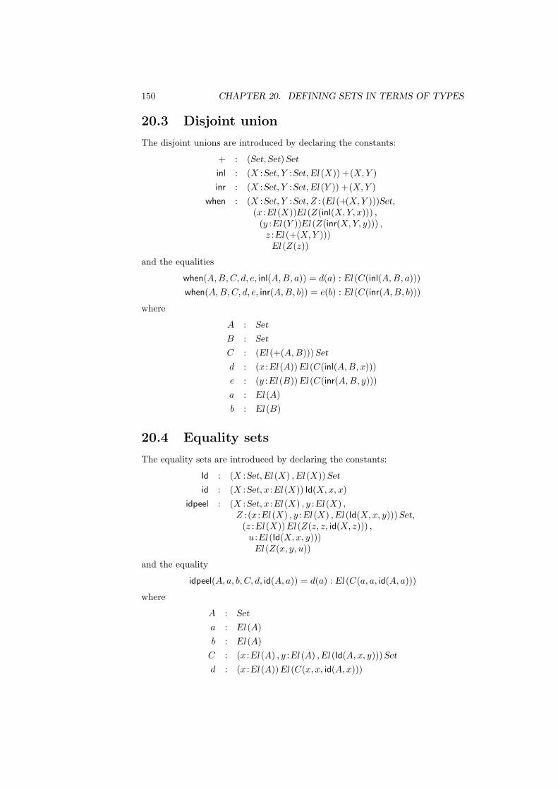
150 CHAPTER 20. DEFINING SETS IN TERMS OF TYPES
20.3 Disjoint union
The disjoint unions are introduced by declaring the constants:
+ : (Set,Set) Set
inl : (X :Set, Y :Set,El (X)) +(X, Y )inr : (X :Set, Y :Set,El (Y )) +(X, Y )
when : (X :Set, Y :Set, Z : (El (+(X, Y )))Set,(x :El (X))El (Z(inl(X, Y, x))) ,
(y :El (Y ))El (Z(inr(X, Y, y))) ,z :El (+(X, Y )))
El (Z(z))
and the equalities
when(A,B, C, d, e, inl(A,B, a)) = d(a) : El (C(inl(A,B, a)))when(A,B,C, d, e, inr(A,B, b)) = e(b) : El (C(inr(A,B, b)))
where
A : Set
B : Set
C : (El (+(A,B)))Set
d : (x :El (A))El (C(inl(A,B, x)))e : (y :El (B))El (C(inr(A,B, y)))a : El (A)b : El (B)
20.4 Equality sets
The equality sets are introduced by declaring the constants:
Id : (X :Set,El (X) ,El (X))Set
id : (X :Set, x :El (X)) Id(X, x, x)idpeel : (X :Set, x :El (X) , y :El (X) ,
Z : (x :El (X) , y :El (X) ,El (Id(X, x, y)))Set,(z :El (X))El (Z(z, z, id(X, z))) ,
u :El (Id(X, x, y)))El (Z(x, y, u))
and the equality
idpeel(A, a, b, C, d, id(A, a)) = d(a) : El (C(a, a, id(A, a)))
where
A : Set
a : El (A)b : El (A)
C : (x :El (A) , y :El (A) ,El (Id(A, x, y)))Set
d : (x :El (A))El (C(x, x, id(A, x)))

20.5. FINITE SETS 151
20.5 Finite sets
We introduce the empty set and the one element set as examples of finite sets.The empty set is introduced by declaring the constants:
{} : Set
case{} : ((Z :El ({}))Set, x :El ({}))El (Z(x))
The one element set is introduced by declaring the constants:
T : Set
tt : El (T))caseT : (Z : (El (T))Set,El (Z(tt)) , x :El (T))El (Z(x))
and the equality
caseT(C, b, tt) = b(tt) : El (C(tt))
where C : (El (T))Set and b : El (C(tt)).
20.6 Natural numbers
The set of natural numbers is introduced by declaring the constants:
N : Set
0 : El (N)succ : (El (N))El (N)
natrec : (Z : (El (N))Set,El (Z(0)) ,
(x :El (N) ,El (Z(x)))El (Z(succ(x))) ,n :El (N))
El (Z(n))
and the equalities
natrec(C, d, e, 0) = d : El (C(0))natrec(C, d, e, succ(a)) = e(a, natrec(C, d, e, a)) : El (C(succ(a)))
where
C : (x :El (N))Set
d : El (C(0))e : (x :El (N) ,El (C(x)))El (C(succ(x)))a : El (N)
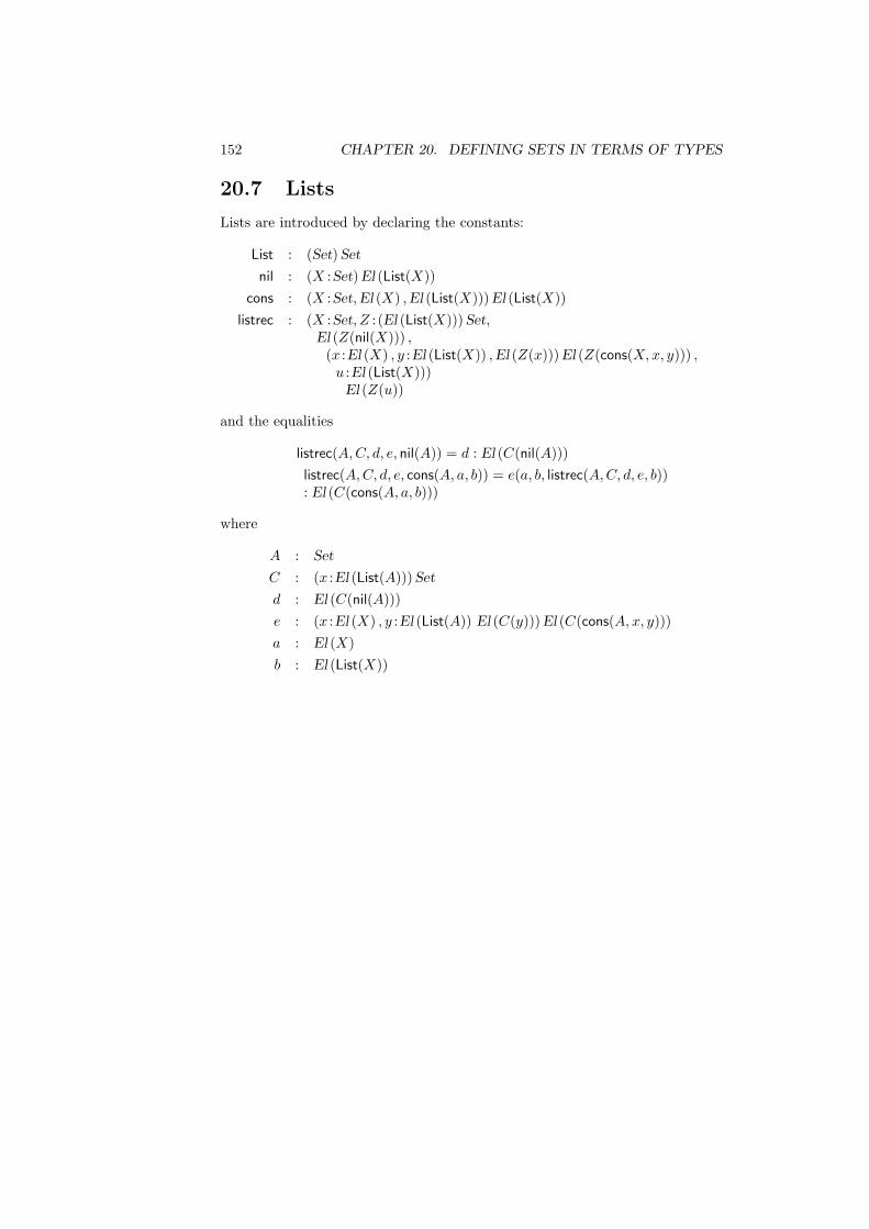
152 CHAPTER 20. DEFINING SETS IN TERMS OF TYPES
20.7 Lists
Lists are introduced by declaring the constants:
List : (Set) Set
nil : (X :Set) El (List(X))cons : (X :Set,El (X) ,El (List(X)))El (List(X))
listrec : (X :Set, Z : (El (List(X)))Set,El (Z(nil(X))) ,
(x :El (X) , y :El (List(X)) ,El (Z(x)))El (Z(cons(X, x, y))) ,u :El (List(X)))
El (Z(u))
and the equalities
listrec(A,C, d, e, nil(A)) = d : El (C(nil(A)))listrec(A,C, d, e, cons(A, a, b)) = e(a, b, listrec(A,C, d, e, b)): El (C(cons(A, a, b)))
where
A : Set
C : (x :El (List(A)))Set
d : El (C(nil(A)))e : (x :El (X) , y :El (List(A)) El (C(y)))El (C(cons(A, x, y)))a : El (X)b : El (List(X))

Part IV
Examples
153


Chapter 21
Some small examples
21.1 Division by 2
In this example we give a derivation of the proposition
(∃y ∈ N)(x =N y ∗ 2)∨ (x =N y ∗ 2⊕ 1) [x ∈ N ] (21.1)
and then by interpreting propositions as sets show how to obtain a programwhich for each natural number n computes the integral part of n/2. In thischapter we are using the infix symbol ⊕ for addition between natural numbers.
We prove (21.1) by induction on x.
Base: By definition of ∗ we have
0 =N 0 ∗ 2
from which we get, by ∨ -introduction and ∃-introduction,
(∃y ∈ N)((0 =N y ∗ 2)∨ (0 =N y ∗ 2⊕ 1))
Induction step: We want to prove
(∃y ∈ N)((x⊕ 1 =N y ∗ 2)∨ (x⊕ 1 =N y ∗ 2⊕ 1))
from the assumptions
x ∈ N, (∃y ∈ N)((x =N y ∗ 2)∨ (x =N y ∗ 2⊕ 1)) (21.2)
We will use ∃-elimination on (21.2) and therefore assume
y ∈ N, x =N y ∗ 2∨x =N y ∗ 2⊕ 1 (21.3)
There are two cases corresponding to the two disjuncts in (21.3):
(i) Assumex =N y ∗ 2 (21.4)
By substitution we get
x⊕ 1 =N y ∗ 2⊕ 1
155
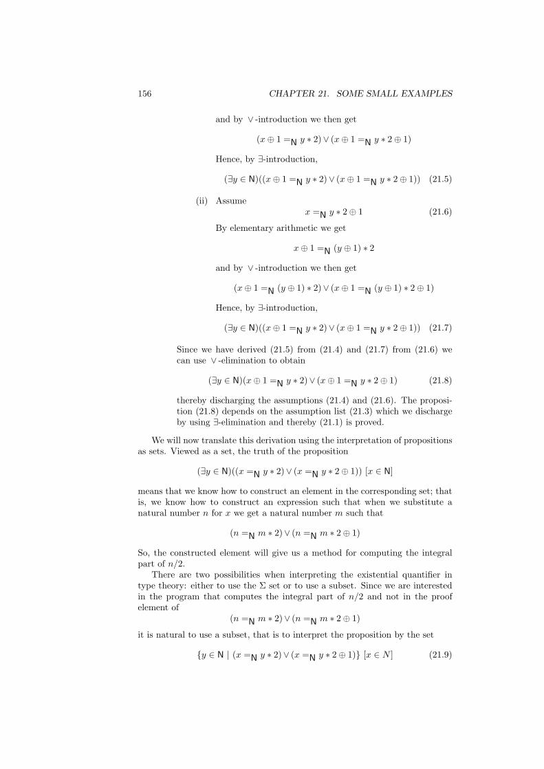
156 CHAPTER 21. SOME SMALL EXAMPLES
and by ∨ -introduction we then get
(x⊕ 1 =N y ∗ 2)∨ (x⊕ 1 =N y ∗ 2⊕ 1)
Hence, by ∃-introduction,
(∃y ∈ N)((x⊕ 1 =N y ∗ 2)∨ (x⊕ 1 =N y ∗ 2⊕ 1)) (21.5)
(ii) Assumex =N y ∗ 2⊕ 1 (21.6)
By elementary arithmetic we get
x⊕ 1 =N (y ⊕ 1) ∗ 2
and by ∨ -introduction we then get
(x⊕ 1 =N (y ⊕ 1) ∗ 2)∨ (x⊕ 1 =N (y ⊕ 1) ∗ 2⊕ 1)
Hence, by ∃-introduction,
(∃y ∈ N)((x⊕ 1 =N y ∗ 2)∨ (x⊕ 1 =N y ∗ 2⊕ 1)) (21.7)
Since we have derived (21.5) from (21.4) and (21.7) from (21.6) wecan use ∨ -elimination to obtain
(∃y ∈ N)(x⊕ 1 =N y ∗ 2)∨ (x⊕ 1 =N y ∗ 2⊕ 1) (21.8)
thereby discharging the assumptions (21.4) and (21.6). The proposi-tion (21.8) depends on the assumption list (21.3) which we dischargeby using ∃-elimination and thereby (21.1) is proved.
We will now translate this derivation using the interpretation of propositionsas sets. Viewed as a set, the truth of the proposition
(∃y ∈ N)((x =N y ∗ 2)∨ (x =N y ∗ 2⊕ 1)) [x ∈ N]
means that we know how to construct an element in the corresponding set; thatis, we know how to construct an expression such that when we substitute anatural number n for x we get a natural number m such that
(n =N m ∗ 2)∨ (n =N m ∗ 2⊕ 1)
So, the constructed element will give us a method for computing the integralpart of n/2.
There are two possibilities when interpreting the existential quantifier intype theory: either to use the Σ set or to use a subset. Since we are interestedin the program that computes the integral part of n/2 and not in the proofelement of
(n =N m ∗ 2)∨ (n =N m ∗ 2⊕ 1)
it is natural to use a subset, that is to interpret the proposition by the set
{y ∈ N | (x =N y ∗ 2)∨ (x =N y ∗ 2⊕ 1)} [x ∈ N ] (21.9)

21.1. DIVISION BY 2 157
However, using the subset it is not possible to directly translate the proof aboveto type theory because subset-elimination is not strong enough to interpret ∃-elimination. So we will instead use the Σ set when translating the proof. Wewill then get an element in the set
(Σy ∈ N)((x =N y ∗ 2) + (x =N y ∗ 2⊕ 1)) [x ∈ N]
and by applying the projection fst on this element we will get a program satis-fying (21.9).
Our proof of
(∃y ∈ N)((x =N y ∗ 2)∨ (x =N y ∗ 2⊕ 1)) [x ∈ N]
was by induction, so we will construct an element of the set
(Σy ∈ N)((x =N y ∗ 2) + (x =N y ∗ 2⊕ 1)) [x ∈ N] (21.10)
by N-elimination, remembering that induction corresponds to N-elimination intype theory.
Base: By N-equality and Id-introduction we have
id(0) ∈ (0 =N 0 ∗ 2)
So, by +-introduction and Σ-introduction, we get
〈0, inl(id(0))〉 ∈ (Σy ∈ N)((0 =N y ∗ 2) + (0 =N y ∗ 2⊕ 1))
Recursion step: We want to construct an element in the set
(Σy ∈ N)((x⊕ 1 =N y ∗ 2) + (x⊕ 1 =N y ∗ 2⊕ 1))
from the assumptions
x ∈ N, z1 ∈ (Σy ∈ N)((x =N y ∗ 2) + (x =N y ∗ 2⊕ 1)) (21.11)
We will use Σ-elimination on (21.11) and therefore assume
y ∈ N, z2 ∈ ((x =N y ∗ 2) + (x =N y ∗ 2⊕ 1)) (21.12)
There are two cases:
(i) Assumez3 ∈ (x =N y ∗ 2) (21.13)
Substitution in the propositional function Id(N, x ⊕ 1, z ⊕1) [z ∈ N] gives
subst(z3, id(x⊕ 1)) ∈ (x⊕ 1 =N y ∗ 2⊕ 1)
and by +-introduction we then get
inr(subst(z3, id(x⊕1))) ∈ (x⊕1 =N y∗2)+(x⊕1 =N y∗2⊕1)
Hence, by Σ-introduction,
〈y, inr(subst(z3, id(x⊕ 1)))〉∈ (Σy ∈ N)((x⊕ 1 =N y ∗ 2)+(x⊕ 1 =N y ∗ 2⊕ 1))
(21.14)

158 CHAPTER 21. SOME SMALL EXAMPLES
(ii) Assumez4 ∈ (x =N y ∗ 2⊕ 1) (21.15)
By elementary arithmetic we get a construction
c(x, y, z4) ∈ (x⊕ 1 =N (y ⊕ 1) ∗ 2)
and by +-introduction we then get
inl(c(x, y, z4)) ∈ (x⊕1 =N (y⊕1)∗2+x⊕1 =N (y⊕1)∗2⊕1)
Hence, by Σ-introduction,
〈y ⊕ 1, inl(c(x, y, z4))〉∈ (Σy ∈ N)((x⊕ 1 =N y ∗ 2)+(x⊕ 1 =N y ∗ 2⊕ 1))
(21.16)
Since we have a derived (21.14) from (21.13) and (21.16) from (21.15)we can use +-elimination to obtain
when(z2,(z3)〈y, inr(subst(z3, id(x⊕ 1)))〉,(z4)〈y ⊕ 1, inl(c(x, y, z4))〉))))
∈ (Σy ∈ N)((x⊕ 1 =N y ∗ 2)+(x⊕ 1 =N y ∗ 2⊕ 1))
(21.17)
thereby discharging assumptions (21.13) and (21.15). (21.16) de-pends on the assumption (21.12) which we can discharge by usingΣ-elimination:
split(z1,(y, z2)when(z2,
(z3)〈y, inr(subst(z3, id(x⊕ 1)))〉,(z4)〈y ⊕ 1, inl(c(x, y, z4))〉))))
∈ (Σy ∈ N)((x⊕ 1 =N y ∗ 2)+(x⊕ 1 =N y ∗ 2⊕ 1))
Now we can use N-elimination to obtain
natrec(x,〈0, inl(id(0))〉,(x, z1)split(z1,
(y, z2)when(z2,(z3)〈y, inr(subst(z3, id(x⊕ 1)))〉,(z4)〈y ⊕ 1, inl(c(x, y, z4))〉))))
∈ (Σy ∈ N)((x =N y ∗ 2)+(x =N y ∗ 2⊕ 1))[x ∈ N]
(21.18)
Defining half proof by
half proof ≡λx.natrec(x,
〈0, inl(id(0))〉,(x, z1)split(z1,
(y, z2)when(z2,(z3)〈y, inr(subst(z3, id(x⊕ 1)))〉,(z4)〈y ⊕ 1, inl(c(x, y, z4))〉)))

21.2. EVEN OR ODD 159
and half byhalf(x) ≡ fst(half proof · x)
we get, by applying Σ-elimination twice and then using subset intro-duction,
half(x) ∈ {y ∈ N|(x =N y ∗ 2) + (x =N y ∗ 2⊕ 1)} [x ∈ N ]
Note that we in this type theory derivation not only have constructed theprogram half but also simultaneously have given an almost formal proof that theprogram satisfies the specification, that is that half(n) computes the integralpart of n/2 for each natural number n.
In the proof there was a proof of a trivial arithmetic equation which wedid not carry out. Note, however, that this proof element is never used in thecomputation of the program half.
Since the program was constructed from a derivation using logic, there occurparts in the program which one normally would not use when constructing theprogram in a traditional way. For instance, the when-part of the program comesfrom an application, in the induction step, of ∨ -elimination where one is usingthe induction hypothesis which tells you that a number is either even or odd.Thinking operationally, one would here probably have used some constructioninvolving if then else .
21.2 Even or odd
By using the previous example and a proof of
((∃x ∈ A)(P (x)∨Q(x)))⊃ ((∃x ∈ A)P (x)∨ (∃x ∈ A)Q(x)) (21.19)
we will derive a program even(n) in the set Bool which has value true if thenatural number n is even and false if n is odd.
This can be proved in the following bottom-up way: By ∃-introduction and∨ -introduction we get
(∃x ∈ A)P (x)∨ (∃x ∈ A)Q(x) [x ∈ A, P (x)]
and(∃x ∈ A)P (x)∨ (∃x ∈ A)Q(x) [x ∈ A, Q(x)]
Now we can use ∨ -elimination to get
(∃x ∈ A)P (x)∨ (∃x ∈ A)Q(x) [x ∈ A, P (x)∨Q(x)]
Finally, by ∃-elimination and ⊃ -introduction we obtain (21.19).Translating this proof, using propositions as sets, gives the following deriva-
tion. By Σ -introduction and + -introduction we get
inl(〈x, u〉) ∈ (Σx ∈ A)P (x) + (Σx ∈ A)Q(x) [x ∈ A, u ∈ P (x)]
and
inr(〈x, v〉) ∈ (Σx ∈ A)Q(x) + (Σx ∈ A)Q(x) [x ∈ A, v ∈ Q(x)]
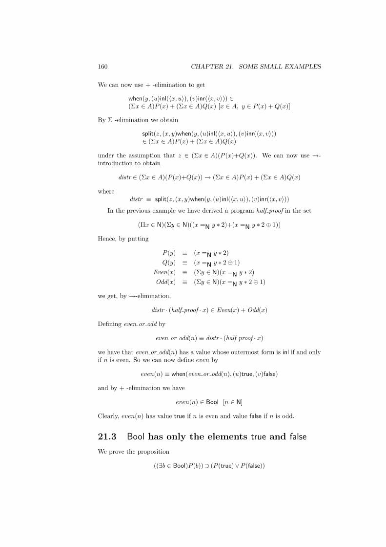
160 CHAPTER 21. SOME SMALL EXAMPLES
We can now use + -elimination to get
when(y, (u)inl(〈x, u〉), (v)inr(〈x, v〉)) ∈(Σx ∈ A)P (x) + (Σx ∈ A)Q(x) [x ∈ A, y ∈ P (x) + Q(x)]
By Σ -elimination we obtain
split(z, (x, y)when(y, (u)inl(〈x, u〉), (v)inr(〈x, v〉))∈ (Σx ∈ A)P (x) + (Σx ∈ A)Q(x)
under the assumption that z ∈ (Σx ∈ A)(P (x)+Q(x)). We can now use →-introduction to obtain
distr ∈ (Σx ∈ A)(P (x)+Q(x)) → (Σx ∈ A)P (x) + (Σx ∈ A)Q(x)
wheredistr ≡ split(z, (x, y)when(y, (u)inl(〈x, u〉), (v)inr(〈x, v〉))
In the previous example we have derived a program half proof in the set
(Πx ∈ N)(Σy ∈ N)((x =N y ∗ 2)+(x =N y ∗ 2⊕ 1))
Hence, by putting
P (y) ≡ (x =N y ∗ 2)Q(y) ≡ (x =N y ∗ 2⊕ 1)
Even(x) ≡ (Σy ∈ N)(x =N y ∗ 2)Odd(x) ≡ (Σy ∈ N)(x =N y ∗ 2⊕ 1)
we get, by →-elimination,
distr · (half proof · x) ∈ Even(x) + Odd(x)
Defining even or odd by
even or odd(n) ≡ distr · (half proof · x)
we have that even or odd(n) has a value whose outermost form is inl if and onlyif n is even. So we can now define even by
even(n) ≡ when(even or odd(n), (u)true, (v)false)
and by + -elimination we have
even(n) ∈ Bool [n ∈ N]
Clearly, even(n) has value true if n is even and value false if n is odd.
21.3 Bool has only the elements true and false
We prove the proposition
((∃b ∈ Bool)P (b))⊃ (P (true)∨P (false))

21.3. BOOL HAS ONLY THE ELEMENTS TRUE AND FALSE 161
by showing that the set
((Σb ∈ Bool)P (b)) → (P (true) + P (false))
is inhabited.We start the derivation by assuming
w ∈ (Σb ∈ Bool)P (b) (21.1)
and then look for an element in the set
P (true) + P (false)
We continue by making two more assumptions
w1 ∈ Bool (21.2)w2 ∈ P (w1) (21.3)
Unfortunately, there is now not a straightforward way to get an element in theset P (true) + P (false) from the assumptions we have introduced. Instead wemust first derive an element in the set
P (w1) → (P (true) + P (false))
by case analysis on w1 and then apply this element on w2 to get an element inthe set
P (true) + P (false)
We use +-introduction and →-introduction on the assumption
q ∈ P (true)
to getλ(inl) ∈ P (true)⊃ (P (true)+P (false)) (21.4)
In the same way we also get
λ(inr) ∈ P (false)⊃ (P (true)+P (false)) (21.5)
By applying Bool-elimination on (21.2), (21.4) and (21.5), we get
if w1 then λ(inl) else λ(inr)∈ P (w1) → (P (true)+P (false)) (21.6)
Then →-elimination, applied on (21.3) and (21.6), gives
apply(if w1 then λ(inl) else λ(inr), w2)∈ P (true)+P (false) (21.7)
Now we can apply the ∃-elimination rule on (21.1) and (21.7) and therebydischarging assumption (21.2) and (21.3):
split(w,(w1, w2)apply(if w1 then λ(inl) else λ(inr),
w2))∈ P (true)+P (false)
(21.8)

162 CHAPTER 21. SOME SMALL EXAMPLES
Finally, by →-introduction, we discharge (21.1) and get
λw.split(w,(w1, w2)apply(if w1 then λ(inl) else λ(inr),
w2))∈ P (true)+P (false)
(21.9)
In essentially the same way we can prove the propositions:
(∃x ∈ N)P (x)⊃ (P (0)∨ (∃y ∈ N)P (succ(y)))(∃x ∈ List(A))P (x)⊃ (P (nil)∨ (∃y ∈ A)(∃z ∈ List(A))P (cons(x, y)))(∃x ∈ A + B)P (x)⊃ ((∃y ∈ A)P (inl(y))∨ (∃z ∈ B)P (inr(z)))(∃x ∈ A×B)P (x)⊃ (∃y ∈ A)(∃z ∈ B)P (〈y, z〉)
21.4 Decidable predicates
The disjoint union can be used to express that a predicate (propositional func-tion) is decidable. Consider the set B(x) set [x ∈ A]. To say that B is decidablemeans that there is a mechanical procedure which for an arbitrary element a ∈ Adecides if B(a) is true or if it is false. In order to formally express that a predi-cate B is decidable for elements from A, one can use the disjoint union. If theset
Decidable(A,B) ≡ (Πx∈A) B(x)∨¬B(x)
is nonempty, then B is decidable and an element in the set is a decision procedurefor the predicate.
As an example of a decidable predicate and a decision procedure, we willshow that there is an element in the set Decidable(N, (n)Id(N, 0, n)), therebygetting a decision procedure that decides if a natural number is equal to zero.We start the derivation by assuming
n ∈ N
We then proceed to find an element in the set
Id(N, 0, n)∨¬Id(N, 0, n)
by induction on n.The base case: By N-introduction, Id-introduction and ∨ -introduction, we
getinl(id(0)) ∈ Id(N, 0, 0)∨¬Id(N, 0, 0)
The induction step: We first introduce the induction assumptions
x ∈ N
y ∈ Id(N, 0, x)∨¬Id(N, 0, x)
and then continue with the assumption
z ∈ Id(N, 0, succ(x))

21.5. STRONGER ELIMINATION RULES 163
By the proof of Peano’s fourth axiom, we have
peano4 ∈ Id(N, 0, succ(n)) → {} [n ∈ N]
By {}-elimination and →-introduction, we get
λ((z)case(peano4 · z)) ∈ ¬Id(N, 0, succ(x))
We can then use ∨ -introduction to get
inr(λ((z)case(peano4 · z)) ∈ Id(N, 0, succ(x))∨¬Id(N, 0, succ(x))
and the N-elimination rule therefore gives us
natrec(n, inl(id(0)), (x, y)inr(λ((z)case(peano4 · z)))) ∈Id(N, 0, n)∨¬Id(N, 0, n)
Finally, by →-introduction,
λ((n)natrec(n, inl(id(0)), (x, y)inr(λ((z)case(peano4 · z)))))∈ Decidable(N, (n)Id(N, 0, n))
So, we have derived a decision procedure for the predicate (n)Id(N, 0, n).
21.5 Stronger elimination rules
It is possible to formulate stronger versions of the elimination rules, for instance,the rule of strong Σ-elimination:
Strong Σ – elimination
c ∈ Σ(A,B)C(v) set [v ∈ Σ(A,B)]d(x, y) ∈ C(〈x, y〉) [x ∈ A, y ∈ B(x), 〈x, y〉 =Σ(A,B) c true]split′(c, d) ∈ C(c)
The third premise is weaker than the corresponding premise in the ordinary rulefor Σ-elimination in that the assumption 〈x, y〉 =Σ(A,B) c true is added. Theconstant split has been replaced by the defined constant split′. This rule can beseen as a derived rule in the following way:
Let
c ∈ Σ(A,B)C(v) set [v ∈ Σ(A,B)]d(x′, y′) ∈ C(〈x′, y′〉) [x′ ∈ A, y′ ∈ B(x′), 〈x′, y′〉 =Σ(A,B) c true]
We are going to use the ordinary Σ-elimination rule on c and the family
C ′(u) ≡ (u =Σ(A,B) c) → C(u)
So, assume x ∈ A and y ∈ B(x) and we want to find an element in
C ′(〈x, y〉) ≡ (〈x, y〉 =Σ(A,B) c) → C(〈x, y〉)

164 CHAPTER 21. SOME SMALL EXAMPLES
Assume therefore that z ∈ (〈x, y〉 =Σ(A,B) c). But then
d(x, y) ∈ C(〈x, y〉)
and →-introduction gives that
λz.d(x, y) ∈ (〈x, y〉 =Σ(A,B) c) → C(〈x, y〉)
thereby discharging the last assumption. Σ-elimination gives
split(c, (x, y)λz.d(x, y)) ∈ (c =Σ(A,B) c) → C(c)
thereby discharging the remaining two assumptions. Since we know that id(c) ∈(c =Σ(A,B) c) we can use →-elimination to finally conclude that
split′(c, d) ∈ C(c)
wheresplit′(c, d) ≡ apply(split(c, (x, y)λz.d(x, y)), id(c)).
Notice, that if the premises of the strong elimination rule hold then thevalue of split′(c, d) is equal to the value of split(c, d) which can be seen from thefollowing computation steps:
c ⇒〈a, b〉 λz.d(a, b) ⇒λz.d(a, b)split(c, (x, y)λz.d(x, y)) ⇒λz.d(a, b) d(a, b) ⇒ q
apply(split(c, (x, y)λz.d(x, y)), id(c)) ⇒ q
We can strengthen the elimination-rules for Π, +, and the enumeration setsin an analogous way:
Strong Π–elimination
c ∈ Π(A,B)C(v) set [v ∈ Π(A,B)]d(y) ∈ C(λ(y)) [y(x) ∈ B(x) [x ∈ A], c =Π(A,B) λ(y) true]funsplit′(c, d) ∈ C(c)
wherefunsplit′(c, d) ≡ apply(funsplit(c, (y)λz.d(y)), id(c))
Strong +–elimination
c ∈ A + B
C(v) set [v ∈ A + B]d(x) ∈ C(inl(x)) [x ∈ A, c =A+B inl(x) true]e(y) ∈ C(inr(y)) [y ∈ B, c =A+B inr(y) true]when′(c, d, e) ∈ C(c)
where
when′(c, d, e) ≡ apply(when(c, (x)λz.d(x), (y)λz.e(y)), id(c))
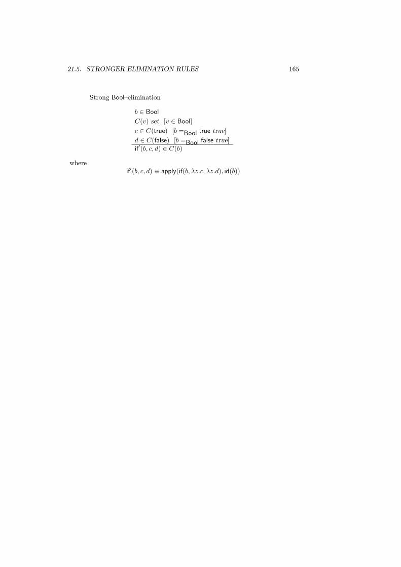
21.5. STRONGER ELIMINATION RULES 165
Strong Bool–elimination
b ∈ Bool
C(v) set [v ∈ Bool]c ∈ C(true) [b =Bool true true]d ∈ C(false) [b =Bool false true]if′(b, c, d) ∈ C(b)
whereif′(b, c, d) ≡ apply(if(b, λz.c, λz.d), id(b))

166 CHAPTER 21. SOME SMALL EXAMPLES

Chapter 22
Program derivation
One of the main reasons for using type theory for programming is that it canbe seen as a theory both for writing specifications and constructing programs.In type theory a specification is expressed as a set and an element of that set isa program that satisfies the specification.
Programming in type theory corresponds to theorem proving in mathemat-ics: the specification plays the role of the proposition to be proved and theprogram is obtained from the proof. We will in this chapter formulate the rulesof type theory as tactics, corresponding to constructing programs top down.The idea of synthesising programs from constructive proofs has been used e.g.by Manna and Waldinger [62] Takasu [106] and Constable and his coworkers atCornell University [25].
22.1 The program derivation method
As already has been mentioned, programming in type theory is like theoremproving in mathematics. However, since parts of the proofs are used in the actualconstruction of programs, the proofs have to be more detailed and formal thanthey usually are in mathematics. In this respect, derivations of programs in typetheory are similar to proofs of mathematical theorems in a formal system. Beingformal is also a necessity when dealing with complex problems since one thencertainly need computer support. For the examples in this chapter the solutionsare so simple that there are no problems in doing the derivations informally.But already in the solution of Dijkstra’s problem of the Dutch national flagusing arrays [87], there are so many steps and so much book-keeping that it isappropriate to make the derivation in such a way that it could be checked bya computer. So, in order to illustrate the method, our example is carried outin such a detail that it should be straightforward to obtain a completely formalderivation. Differences between proofs in traditional mathematics and programderivations as well as the role of formalization are discussed by Scherlis andScott [94].
The usual way of presenting a formal derivation, e.g. in text books onlogic, is to go from axioms and assumptions to the conclusion. When derivingprograms in type theory this would mean that you first start constructing thesmaller parts of the program and then build up the program from these parts.
167

168 CHAPTER 22. PROGRAM DERIVATION
This is not a good programming methodology. Instead we want to use thetop-down approach from structured programming [32]. So, instead of startingthe derivation from axioms and assumptions, we will proceed in the oppositedirection. We will start with the specification, split it into subspecificationsand then compose solutions to these subproblems to a solution of the originalproblem. In the LCF-system [44] there is a goal directed technique for findingproofs in this style.
Corresponding to the judgement
a ∈ A
we have the goal A which is achieved by an element a if we have a proof of a ∈ A.Corresponding to each of the other forms of judgement, we have a goal whichhas the same form as the judgement and which is achieved if we have a proof ofit. For instance the goal a = b ∈ A is achieved if we have a proof of a = b ∈ A.Notice that in general goals may depend on assumptions. The different methodsthat can be used to split a goal into subgoals are called tactics.
22.1.1 Basic tactics
The basic tactics come from reading the rules of type theory bottom-up. Forexample, the introduction rule for conjunction
A true B true
A &B true
becomes, when viewed as a tactic:
The goalA &B true
may be split into the subgoals
A true
andB true
We can describe the tactic in the following way:
dA &B true by & -introduction[A true by ...[B true by ...
b
Similarly, the introduction rule for the cartesian product
a ∈ A b ∈ B
〈a, b〉 ∈ A &B
can be read as a tactic:

22.1. THE PROGRAM DERIVATION METHOD 169
The problem of finding a program that achieves the goal
A×B
can be split into the problem of finding a program a that achievesthe goal
A
and the problem of finding a program b that achieves the goal
B
The goal A×B is then achieved by the program 〈a, b〉.
When deriving a program from a specification, applying a tactic will give apart of the program one is in the process of constructing. In the case of the×-introduction tactic, one gets a part on pair-form. The ×-introduction tacticcan also be described in the following way:
dA×B by ×-introductiondA by ...b3 adB by ...b3 b
b3 〈a, b〉
This schematical way of describing a tactic can be extended to full derivations.It can also be used when a derivation is not yet complete and then give thestructure of the derivation made so far as well as the structure of the programobtained at that stage.
Another example is the rule for ×-elimination:
p ∈ A×B e(x, y) ∈ C(〈x, y〉 [x ∈ A, y ∈ B]split(p, e) ∈ C(p)
we get the following ×-elimination tactic in type theory:
The problem of finding a program that achieves the goal
C(p)
can be replaced by proving that p ∈ A×B and the problem of findinga program e(x, y) that achieves the goal
C(〈x, y〉)
under the assumptions that x ∈ A and y ∈ B.
The goal C(p) is then achieved by the program split(p, e).
In our notation:
dC(p) by ×-eliminationdA×B by ...b3 p[x ∈ A, y ∈ B]
dC(〈x, y〉) by ...b3 e(x, y)
b3 split(p, e)

170 CHAPTER 22. PROGRAM DERIVATION
In this way all rules of type theory may be formulated as tactics. This is also theapproach taken in the system for type theory developed at Cornell University[25]. We give two more examples of translating rules into tactics by formulatingthe Π-introduction rule and the List-elimination rule as tactics. Both tacticswill be used in the derivation of a program for the problem of the Dutch flag.
Corresponding to the Π-introduction rule
b(x) ∈ B(x) [x ∈ A]λ(b) ∈ (Πx ∈ A)B(x)
we have the tactic:
d(Πx ∈ A) B(x) by Π-introduction[x ∈ A]
dB(x) by ...b3 b(x)
b3 λ(b)
The List-elimination rule,
l ∈ List(A)a ∈ C(nil)b(x, y, z) ∈ C(cons(x, y)) [x ∈ A, y ∈ List(A), z ∈ C(y)]
listrec(l, a, b) ∈ C(l)
becomes, when formulated as a tactic:
dC(l) by List-eliminationdList(A) by ...b3 ldC(nil) by ...b3 a[x ∈ A, y ∈ List(A), z ∈ C(y)]
dC(cons(x, y)) by ...b3 b(x, y, z)
b3 listrec(l, a, b)
22.1.2 Derived tactics
If we have a proof of a judgement then we also have a derived tactic corre-sponding to the judgement. We can look at a tactic as another way of readinga hypothetical judgement. For instance, if we have a proof of the hypotheticaljudgement
c(x, y) ∈ C(x, y) [x ∈ A, y ∈ B(x)] (J1)
then we can use the following tactic:
dC(x, y) by J1dA by ...b3 xdB(x) by ...b3 y
b3 c(x, y)

22.2. A PARTITIONING PROBLEM 171
As a simple example, after having made the derivation
[p ∈ A×B]dA by ×-elimination
dA×B by assumptionb3 p[x ∈ A, y ∈ B]
dA by assumptionb3 x
b3 split(p, (x, y)x) ≡ fst(p)
which is a proof of the judgement
fst(p) ∈ A [p ∈ A×B] (×− elim1)
[p ∈ A×B]dA by ×-elim1b3 fst(p)
If we had a mechanical proof checker, it would not be necessary to check thecorrectness of a derived tactic more than once. In an application of it, thereis no need to go through each step in the proof since by the construction of aderived tactic (that it comes from a judgement) we know that if we apply it toproofs of the subgoals it always yield a proof of the goal.
22.2 A partitioning problem
In this section, we will derive a program for Dijkstra’s problem of the Dutchnational flag [32]: Construct a program, that given a sequence of objects, eachhaving one of the colours red, white and blue, rearranges the objects so that theyappear in the order of the Dutch national flag. In type theory, the natural wayof formulating this partitioning problem is to use lists. Our solution will then,we think, result in the simplest possible program for the problem; the programone would write in a functional language like ML. However, the program willnot satisfy Dijkstra’s requirements concerning space efficiency, which is one ofthe main points of his solution. In [87] a similar problem is solved, using arraysinstead of lists and following Dijkstra’s more sophisticated method.
We will use the following general assumptions about the problem: We assumethat A is a set and each element in A has a colour, i.e. there is a functioncolour(x) ∈ Colour, where Colour is the enumeration set {red,white, blue}. Wewill also assume that A has a decidable equality. So we introduce the followingassumptions:
A setcolour(x) ∈ Colour [x ∈ A]eqd(A, x, y) ∈ {z ∈ Bool | z =Bool true ⇔ x =A y} [x ∈ A, y ∈ A]

172 CHAPTER 22. PROGRAM DERIVATION
We start by introducing the following definitions:
Colouredlist(s) ≡ List({x ∈ A | colour(x) =Colour s})Reds ≡ Colouredlist(red)
Whites ≡ Colouredlist(white)Blues ≡ Colouredlist(blue)
append(l1, l2) ≡ listrec(l1, l2, (x, y, z) cons(x, z))l1 ≈P l2 ≡ (∀x∈A) Id(N, occin(x, l1), occin(x, l2))
occin(x, l) ≡ listrec(l, 0, (u, v, w) if eqd(A, x, u) then succ(w) else w)l1@l2 ≡ append(l1, l2)
We have here used a definition of permutation which requires the equality rela-tion on A to be decidable. This restriction can be removed, but the definitionwill then be more complicated.
The specification can now be given by the set
S ≡ (Π l∈List(A)) Flag(l)
where
Flag(l) ≡ {〈l′, l′′, l′′′〉 ∈ Reds×Whites×Blues | l ≈P l′@l′′@l′′′}
using the notation {〈x, y, z〉 ∈ A×B×C | P (x, y, z)} for the subset
{u ∈ A×(B×C) | P (fst(u), fst(snd(u)), trd(u))}
where trd is defined bytrd ≡ (u)snd(snd(u))
Note that a program that satisfies this specification will give a triple of lists asoutput. To get a solution to Dijkstra’s formulation of the problem, these threelists should be concatenated.
Deriving a program that satisfies the specification is nothing but finding aprogram which is a member of the set expressing the specification, or, if wethink of the specification as a goal, to find a program that achieves the goal.
The intuitive idea behind the proof is the following: If l is a list of red,white and blue objects then the problem of finding an element in Flag(l) willbe solved by induction on l. The base case, i.e. when l is equal to nil, is solvedby the partition 〈nil, nil, nil〉. For the induction step, assume that l is cons(x, y)and that we have a partitioning z of y and then separate the problem into threecases:
1. x is red. Then 〈cons(x, fst(z)), snd(z), trd(z)〉 is a partitioning of the listcons(x, y).
2. x is white. Then 〈fst(z), cons(x, snd(z)), trd(z)〉 is a partitioning of the listcons(x, y).
3. x is blue. Then 〈fst(z), snd(z), cons(x, trd(z))〉 is a partitioning of the listcons(x, y).
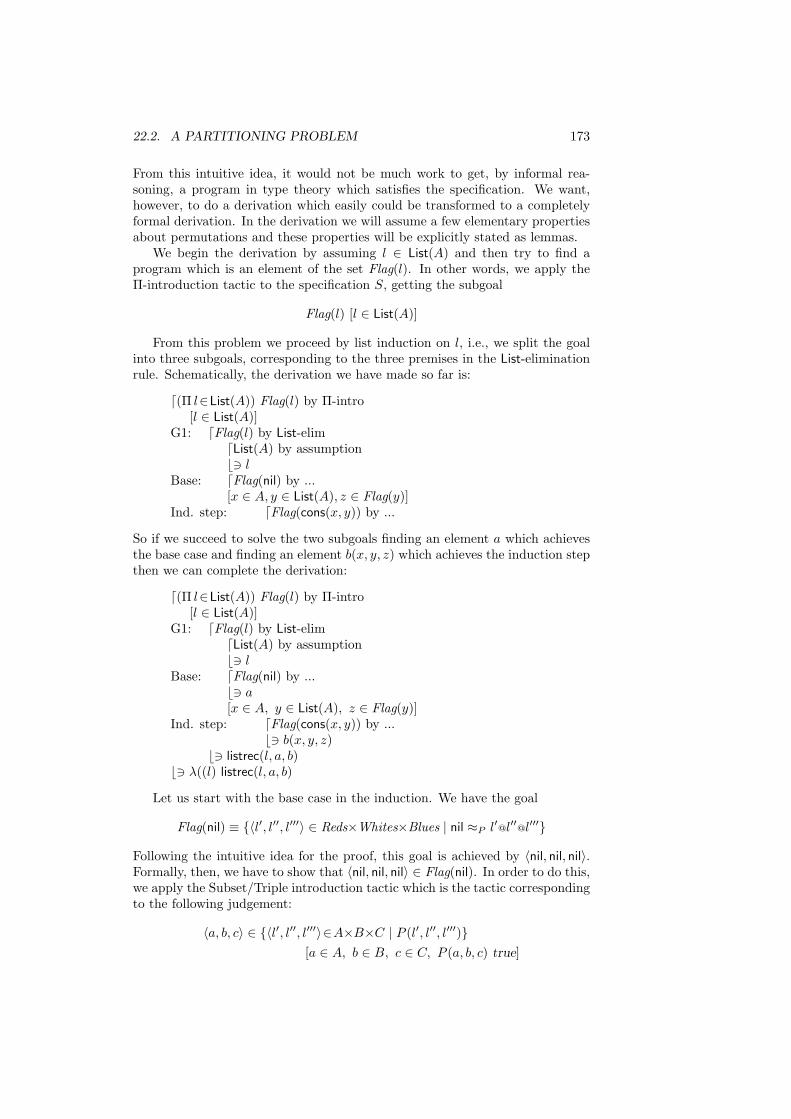
22.2. A PARTITIONING PROBLEM 173
From this intuitive idea, it would not be much work to get, by informal rea-soning, a program in type theory which satisfies the specification. We want,however, to do a derivation which easily could be transformed to a completelyformal derivation. In the derivation we will assume a few elementary propertiesabout permutations and these properties will be explicitly stated as lemmas.
We begin the derivation by assuming l ∈ List(A) and then try to find aprogram which is an element of the set Flag(l). In other words, we apply theΠ-introduction tactic to the specification S, getting the subgoal
Flag(l) [l ∈ List(A)]
From this problem we proceed by list induction on l, i.e., we split the goalinto three subgoals, corresponding to the three premises in the List-eliminationrule. Schematically, the derivation we have made so far is:
d(Π l∈List(A)) Flag(l) by Π-intro[l ∈ List(A)]
G1: dFlag(l) by List-elimdList(A) by assumptionb3 l
Base: dFlag(nil) by ...[x ∈ A, y ∈ List(A), z ∈ Flag(y)]
Ind. step: dFlag(cons(x, y)) by ...
So if we succeed to solve the two subgoals finding an element a which achievesthe base case and finding an element b(x, y, z) which achieves the induction stepthen we can complete the derivation:
d(Π l∈List(A)) Flag(l) by Π-intro[l ∈ List(A)]
G1: dFlag(l) by List-elimdList(A) by assumptionb3 l
Base: dFlag(nil) by ...b3 a[x ∈ A, y ∈ List(A), z ∈ Flag(y)]
Ind. step: dFlag(cons(x, y)) by ...b3 b(x, y, z)
b3 listrec(l, a, b)b3 λ((l) listrec(l, a, b)
Let us start with the base case in the induction. We have the goal
Flag(nil) ≡ {〈l′, l′′, l′′′〉 ∈ Reds×Whites×Blues | nil ≈P l′@l′′@l′′′}
Following the intuitive idea for the proof, this goal is achieved by 〈nil, nil, nil〉.Formally, then, we have to show that 〈nil, nil, nil〉 ∈ Flag(nil). In order to do this,we apply the Subset/Triple introduction tactic which is the tactic correspondingto the following judgement:
〈a, b, c〉 ∈ {〈l′, l′′, l′′′〉∈A×B×C | P (l′, l′′, l′′′)}[a ∈ A, b ∈ B, c ∈ C, P (a, b, c) true]
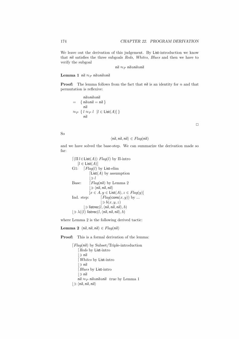
174 CHAPTER 22. PROGRAM DERIVATION
We leave out the derivation of this judgement. By List-introduction we knowthat nil satisfies the three subgoals Reds, Whites, Blues and then we have toverify the subgoal
nil ≈P nil@nil@nil
Lemma 1 nil ≈P nil@nil@nil
Proof: The lemma follows from the fact that nil is an identity for @ and thatpermutation is reflexive:
nil@nil@nil= { nil@nil = nil }
nil≈P { l ≈P l [l ∈ List(A)] }
nil
2
So〈nil, nil, nil〉 ∈ Flag(nil)
and we have solved the base-step. We can summarize the derivation made sofar:
d(Π l∈List(A)) Flag(l) by Π-intro[l ∈ List(A)]
G1: dFlag(l) by List-elimdList(A) by assumptionb3 l
Base: dFlag(nil) by Lemma 2b3 〈nil, nil, nil〉[x ∈ A, y ∈ List(A), z ∈ Flag(y)]
Ind. step: dFlag(cons(x, y)) by ...b3 b(x, y, z)
b3 listrec(l, 〈nil, nil, nil〉, b)b3 λ((l) listrec(l, 〈nil, nil, nil〉, b)
where Lemma 2 is the following derived tactic:
Lemma 2 〈nil, nil, nil〉 ∈ Flag(nil)
Proof: This is a formal derivation of the lemma:
dFlag(nil) by Subset/Triple-introductiondReds by List-introb3 nildWhites by List-introb3 nildBlues by List-introb3 nilnil ≈P nil@nil@nil true by Lemma 1
b3 〈nil, nil, nil〉
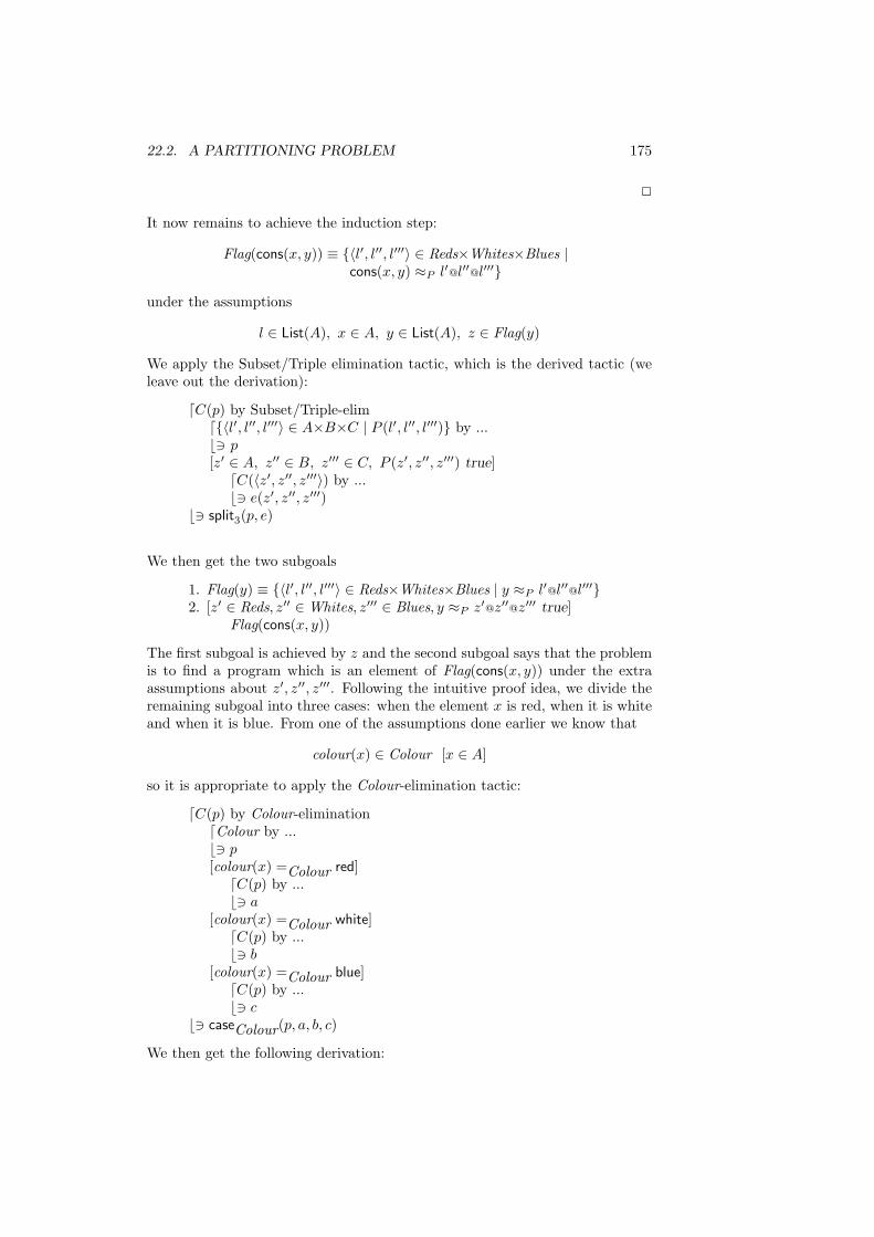
22.2. A PARTITIONING PROBLEM 175
2
It now remains to achieve the induction step:
Flag(cons(x, y)) ≡ {〈l′, l′′, l′′′〉 ∈ Reds×Whites×Blues |cons(x, y) ≈P l′@l′′@l′′′}
under the assumptions
l ∈ List(A), x ∈ A, y ∈ List(A), z ∈ Flag(y)
We apply the Subset/Triple elimination tactic, which is the derived tactic (weleave out the derivation):
dC(p) by Subset/Triple-elimd{〈l′, l′′, l′′′〉 ∈ A×B×C | P (l′, l′′, l′′′)} by ...b3 p[z′ ∈ A, z′′ ∈ B, z′′′ ∈ C, P (z′, z′′, z′′′) true]
dC(〈z′, z′′, z′′′〉) by ...b3 e(z′, z′′, z′′′)
b3 split3(p, e)
We then get the two subgoals
1. Flag(y) ≡ {〈l′, l′′, l′′′〉 ∈ Reds×Whites×Blues | y ≈P l′@l′′@l′′′}2. [z′ ∈ Reds, z′′ ∈ Whites, z′′′ ∈ Blues, y ≈P z′@z′′@z′′′ true]
Flag(cons(x, y))
The first subgoal is achieved by z and the second subgoal says that the problemis to find a program which is an element of Flag(cons(x, y)) under the extraassumptions about z′, z′′, z′′′. Following the intuitive proof idea, we divide theremaining subgoal into three cases: when the element x is red, when it is whiteand when it is blue. From one of the assumptions done earlier we know that
colour(x) ∈ Colour [x ∈ A]
so it is appropriate to apply the Colour-elimination tactic:
dC(p) by Colour-eliminationdColour by ...b3 p[colour(x) =Colour red]
dC(p) by ...b3 a
[colour(x) =Colour white]dC(p) by ...b3 b
[colour(x) =Colour blue]dC(p) by ...b3 c
b3 caseColour(p, a, b, c)
We then get the following derivation:

176 CHAPTER 22. PROGRAM DERIVATION
dFlag(cons(x, y)) by Colour-eliminationdColour by assumptionb3 colour(x)[colour(x) =Colour red]
dFlag(cons(x, y) by ...[colour(x) =Colour white]
dFlag(cons(x, y) by ...[colour(x) =Colour blue]
dFlag(cons(x, y) by ...
That the program〈cons(x, z′), z′′, z′′′〉
achieves the red case is seen by the following derivation, which we call A1.
dFlag(cons(x, y)) ≡{〈l′, l′′, l′′′〉 ∈ Reds×Whites×Blues | cons(x, y) ≈P l′@l′′@l′′′}by Subset/Triple-introdReds ≡ List({x∈A | colour(x) = red}) by List-intro
d{x∈A | colour(x) = red} by subset-introdA by assumptionb3 xdcolour(x) = red true by assumptionb
b3 xd{x∈A | colour(x) = red} by assumptionb3 z′
b3 cons(x, z′)dWhites by assumptionb3 z′′
dBlues by assumptionb3 z′′′
dcons(x, z′)@z′′@z′′′ ≈P cons(x, y) true by Lemma 3b
b3 〈cons(x, z′), z′′, z′′′〉
The following lemma has been used in the derivation.
Lemma 3 If A is a set, x ∈ A, y ∈ List(A), z′ ∈ List(A), z′′ ∈ List(A),z′′′ ∈ List(A) and y ≈P z′@z′′@z′′′ true, then
cons(x, z′)@z′′@z′′′ ≈P cons(x, y) true
Proof: cons(x, z′)@z′′@z′′′
= { List− equality }cons(x, z′@z′′@z′′′)
≈P { z′@z′′@z′′′ ≈P y, cons(x, z) ≈P cons(x, y) [x ∈ A, z ≈P y true] }cons(x, y)
2
We can achieve the remaining subgoals in a similar way, letting A2 and A3correspond to A1 in the white and blue cases, respectively:

22.2. A PARTITIONING PROBLEM 177
dFlag(cons(x, y)) by Colour-eliminationdColour by assumptionb3 colour(x)[colour(x) =Colour red]
dFlag(cons(x, y)) by A1b3 〈cons(x, z′), z′′, z′′′〉
[colour(x) =Colour white]dFlag(cons(x, y) by A2b3 〈z′, cons(x, z′′), z′′′〉
[colour(x) =Colour blue]dFlag(cons(x, y) by A3b3 〈z′, z′′, cons(x, z′′′)〉
Combining the solutions of the last three subproblems gives us that the goalis achieved by
caseColour(colour(x),〈cons(x, z′), z′′, z′′′〉,〈z′, cons(x, z′′), z′′′〉,〈z′, z′′, cons(x, z′′′)〉)
We can now form a program that achieves the induction step:
split3(z,(z′, z′′, z′′′)caseColour(colour(x),
〈cons(x, z′), z′′, z′′′〉,〈z′, cons(x, z′′), z′′′〉,〈z′, z′′, cons(x, z′′′)〉))
G1 is then achieved by
listrec(l, 〈nil, nil, nil〉(x, y, z)split3(z,
(z′, z′′, z′′′)caseColour(colour(x),〈cons(x, z′), z′′, z′′′〉,〈z′, cons(x, z′′), z′′′〉,〈z′, z′′, cons(x, z′′′)〉)))
And, finally
λ((l) listrec(l, 〈nil, nil, nil〉(x, y, z)split3(z,
(z′, z′′, z′′′)caseColour(colour(x),〈cons(x, z′), z′′, z′′′〉,〈z′, cons(x, z′′), z′′′〉,〈z′, z′′, cons(x, z′′′)〉))))
is a program that achieves our original problem and consequently also a programthat satisfies the specification.
The whole derivation is described in figure 22.1.

178 CHAPTER 22. PROGRAM DERIVATION
d(Π l∈List(A)) Flag(l) by Π-intro[l ∈ List(A)]
G1: dFlag(l) by List-elimdList(A) by assumptionb3 l
Base: dFlag(nil) by Lemma 2b3 〈nil, nil, nil〉[x ∈ A, y ∈ List(A), z ∈ Flag(y)]
Ind. step: dFlag(cons(x, y)) by Subset/Triple-elimdFlag(y) ≡{〈l′, l′′, l′′′〉 ∈ Reds×Whites×Blues | y ≈P l′@l′′@l′′′} by ass.b3 z[z′ ∈ Reds, z′′ ∈ Whites, z′′′ ∈ Blues, y ≈P z′@z′′@z′′′ true]
dFlag(cons(x, y)) by Colour-eliminationdColour by assumptionb3 colour(x)[colour(x) =Colour red]
dFlag(cons(x, y)) by A1b3 〈cons(x, z′), z′′, z′′′〉
[colour(x) =Colour white]dFlag(cons(x, y) by A2b3 〈z′, cons(x, z′′), z′′′〉
[colour(x) =Colour blue]dFlag(cons(x, y) by A3b3 〈z′, z′′, cons(x, z′′′)〉
b3 caseColour(colour(x),〈cons(x, z′), z′′, z′′′〉,〈z′, cons(x, z′′), z′′′〉,〈z′, z′′, cons(x, z′′′)〉)
b3 split3(z,(z′, z′′, z′′′)caseColour(colour(x), 〈cons(x, z′), z′′, z′′′〉,
〈z′, cons(x, z′′), z′′′〉,〈z′, z′′, cons(x, z′′′)〉))
b3 listrec(l, 〈nil, nil, nil〉,(x, y, z)split3(z,
(z′, z′′, z′′′)caseColour(colour(x), 〈cons(x, z′), z′′, z′′′〉,〈z′, cons(x, z′′), z′′′〉,〈z′, z′′, cons(x, z′′′)〉)))
b3 λ((l) listrec(l, 〈nil, nil, nil〉,(x, y, z)split3(z,
(z′, z′′, z′′′)caseColour(colour(x), 〈cons(x, z′), z′′, z′′′〉,〈z′, cons(x, z′′), z′′′〉,〈z′, z′′, cons(x, z′′′)〉)))
Figure 22.1: Derivation of a program for the Dutch flag

Chapter 23
Specification of abstractdata types
During the last 10 years, programmers have become increasingly aware of thepractical importance of what Guttag [47] and others have called abstract datatype specifications. A module is a generalization of an abstract data type. It isa tuple
〈A1, A2, . . . , An〉
where some Ai are sets and some are functions and constants defined on thesesets. It is a dependent tuple in the sense that the set that a component belongsto in general can depend on previous components in the tuple. The classicalprogramming example of a module is a stack which is a set together with someoperations defined on the set. An example from mathematics is a group
〈G, ∗, inv, u〉
where G is a set, ∗ ∈ G×G → G, inv ∈ G → G, u ∈ G and certain relationshipshold between the components.
In this section, we will show how to completely specify modules in typetheory using the set of small sets and the dependent sets. We will have a fifthreading of the judgement A set :
A is a module specification
and also a fifth reading of a ∈ A :
a is an implementation of the module specification A
By an abuse of notation, we will not distinguish between sets and theircodings in a universe. We will therefore write A instead of A and not use thefunction Set explicitly. It is always obvious from the context if an expressionrefers to a set or its corresponding element in U.
A simple example is the specification of a stack which in type theory isexpressed by the following set:
179

180 CHAPTER 23. SPECIFICATION OF ABSTRACT DATA TYPES
(ΣStackN ∈ U)(Σempty ∈ StackN)(Σpush ∈ N × StackN → StackN)(Σpop∈StackN → StackN)(Σtop∈StackN → N)
(Πt∈StackN)(Πn∈N)([pop · empty =StackN empty] ×[pop · (push · 〈n, t〉) =StackN t] ×[top · empty =StackN 0] ×[top · (push · 〈n, t〉) =N n])
Using the logical notation for some of the sets, the specification can bereformulated to something that resembles an algebraic specification [47] butwith a completely different semantic explanation:
(∃StackN ∈ U)(∃empty ∈ StackN)(∃push ∈ N× StackN → StackN)(∃pop ∈ StackN → StackN)(∃top∈StackN → N)
(∀t∈StackN)(∀n∈N)([pop · empty =StackN empty] &[pop · (push · 〈n, t〉) =StackN t] &[top · empty =StackN 0] &[top · (push · 〈n, t〉) =N n])
The semantic explanation of this set is an instance of the general schema forexplaining the meaning of a set in terms of canonical expressions and theirequality relation. The canonical expressions of the set (ΣStackN ∈ U) B1 areordered pairs 〈st, b1〉, where st ∈ U and b1 ∈ B1[StackN := st]. Since B1 is alsoa Σ-set, the canonical objects of B1 must also be ordered pairs 〈es, b2〉, wherees ∈ Set(st) and b2 ∈ B2, and so on. If each part of the set is analyzed withrespect to its semantic explanation, one can see that each member of the setmust be equal to a tuple:
〈st, es, pu, po, to, p〉
where〈a, ..., b, c〉 ≡ 〈a, 〈..., 〈b, c〉〉〉
and
st ∈ Ues ∈ Set(st)pu ∈ N× Set(st) → Set(st)po ∈ Set(st) → Set(st)to ∈ Set(st) → Np ∈ (∀t∈Set(st))(∀n∈N) [po · es =Type(st) es]× [. . . ]× [. . .]× [. . .]
Notice that the first component is an element in the set of small sets. This is ofcourse a limitation, we would like to allow an arbitrary set. This could be done,but then we must use something like a Σ-type-forming operation on the level oftypes. The last judgement expresses that st, es, pu and to have the propertiesrequired for the stack operations. So the semantics of the specification is given

23.1. PARAMETERIZED MODULES 181
in terms of the canonical expressions of the set, or, in other words, in terms ofthe correct (canonical) implementations of the specification. The specificationexpresses requirements on implementations of the specification and it is, ofcourse, possible to have requirements which cannot be satisfied. In type theory,a specification with such requirements does not cause any harm; the result isjust that it is impossible to find an implementation for it. It is sometimeseven possible to show that a specification never can be satisfied by proving itequivalent to the empty set.
In the stack specification given above, we specified modules which are equalto objects:
〈st, es, pu, po, to, p〉
where the last component
p ∈ (∀s∈Set(st))(∀n∈N)[po · es =Set(st) es]× [. . . ]× [. . .]× [. . .]
only contains information obtained from the proof that the previous compo-nents of the tuple have the properties required for a stack. This component iscomputationally uninteresting, and if we use a subset instead of a Σ-set we havea specification of a stack without the irrelevant last component:
(Σ StackN ∈ U)(Σempty ∈ StackN)(Σpush ∈ N× StackN → StackN)(Σpop ∈ StackN → StackN){top ∈ StackN → N |
(∀t∈StackN)(∀n∈N)([pop · empty =StackN empty] &[pop · (push · 〈n, t〉) =StackN t] &[top · empty =StackN 0] &[top · (push · 〈n, t〉) =N n])}
As expected, this is a specification of a module which is equal to a 5-tuple:
〈st, es, pu, po, to〉
whose components have the properties we require for a stack.A small problem with this approach is that the equality we get between
stacks is the equality of the implementation of the stack. At the same time aswe specify a stack we would like to have the possibility to express that two stacksare considered equal when they are observationally equal, i.e. when they cannotbe distinguished by any operation defined on stacks. This needs something likea quotient set forming operation, which redefines the equality on a set. Thiswould be a major change in the set theory and we will not explore it furtherhere.
23.1 Parameterized modules
Specifications of parameterized modules, such as a stack of A elements, for anarbitrary set A, are neatly handled in type theory. The parameterized moduleis specified by means of the Π-set former. The specification is the set

182 CHAPTER 23. SPECIFICATION OF ABSTRACT DATA TYPES
STACK ≡(ΠA∈U) in logical notation: (∀A∈U)
(ΣStack ∈ U)(Σempty ∈ Stack)(Σpush ∈ Set(A)× Stack → Stack)(Σpop ∈ Stack → Stack)
...
The canonical expressions of a set (ΠA ∈ U) B are functions λx.s, such thatwhenever they are applied to an object C ∈ U, they will yield an object inthe set B[A := C]. This means that an implementation of the specificationSTACK is a function, which when applied to an element A of the set U returnsan implementation of a stack of A elements. So, if st ∈ STACK , then st · N is amodule of stacks of natural numbers and st · N×N is a module of stacks of pairsof natural numbers. These modules can then be decomposed in the same wayas earlier to get their components.
23.2 A module for sets with a computable equal-ity
The module〈X, e〉
is a computable equality if X is (a coding of) a set and e is a boolean functioncomputing the equality defined on X, i.e.
e · 〈x, y〉 =Bool true, if and only if x =X y
This can be specified by the set
CompEq ≡(ΣX∈U)
{e ∈ X ×X → Bool |(∀y, z∈X)([e · 〈y, z〉 =Bool true ] ⇔ [y =X z])}
Notice that the specification expresses exactly the requirements on the functione, an arbitrary boolean valued function will not do!
We can now use this module specification to define a module FSET for finitesets:
FSET ≡(ΠA∈CompEq)
(ΣFSet ∈ U)(Σeset ∈ FSet)(Σadd ∈ A1 × FSet → FSet){mem ∈ A1 × FSet → Bool |
(∀t∈FSet)(∀a∈A1)(∀b∈A1)([mem · 〈a, eset〉 =Bool false] &[mem · 〈a, add · 〈b, t〉〉 =Bool
if A2 · 〈a, b〉 then true else mem · 〈a, t〉]}

23.2. A MODULE FOR SETS WITH A COMPUTABLE EQUALITY 183
An object of this set is a function which when applied to an object 〈A, e〉 inCompEq yields an implementation of FSET for the particular arguments cho-sen. Note how the Π set-former is used for specifying a dependent function set,in which the elements are functions for which the value of the first argumentsdetermines which set the second argument should be a member of.

184 CHAPTER 23. SPECIFICATION OF ABSTRACT DATA TYPES

Bibliography
[1] Peter Aczel. The Type Theoretic Interpretation of Constructive Set The-ory. In Logic Colloquium ’77, pages 55–66, Amsterdam, 1978. North-Holland Publishing Company.
[2] Peter Aczel. The Type Theoretic Interpretation of Constructive Set The-ory: Choice Principles. In The L. E. J. Brouwer Centenary Symposium,pages 1–40. North-Holland Publishing Company, 1982.
[3] Peter Aczel. The Type Theoretic Interpretation of Constructive Set The-ory: Inductive Definitions. In Logic, Methodology and Philosophy of Sci-ence VII, pages 17–49. Elsevier Science Publishing B.V., 1986.
[4] L. Augustsson and T. Johnsson. The Chalmers Lazy-ML Compiler. TheComputer Journal, 32(2):127 – 141, 1989.
[5] Roland Backhouse. Algorithm Development in Martin-Lof’s Type Theory.Technical report, University of Essex, 1985.
[6] Roland Backhouse, Paul Chisholm, Grant Malcolm, and Erik Saaman.Do-it-yourself type theory. Formal Aspects of Computing, 1:19–84, 1989.
[7] Roland C. Backhouse. Program Construction and Verification. Prentice-Hall, 1986.
[8] Joseph L. Bates and Robert L. Constable. Proofs as Programs. ACMTrans. Prog. Lang. Sys., 7(1):113–136, 1985.
[9] M. J. Beeson. Foundations of Constructive Mathematics. Springer-Verlag,New York, 1985.
[10] Errett Bishop. Foundations of Constructive Analysis. McGraw-Hill, NewYork, 1967.
[11] Errett Bishop. Mathematics as a numerical language. In Myhill, Kino, andVesley, editors, Intuitionism and Proof Theory, pages 53–71, Amsterdam,1970. North Holland.
[12] Errett Bishop and Douglas Bridges. Constructive Analysis. Springer-Verlag, New York, 1985.
[13] Bror Bjerner. Verifying some Efficient Sorting Strategies in Type Theory.PMG Memo 26, Chalmers University of Technology, S–412 96 Goteborg,January 1985.
185

186 BIBLIOGRAPHY
[14] Bror Bjerner. Time Complexity of Programs in Type Theory. PhD thesis,Dept. of Computer Science, University of Goteborg, Goteborg, Sweden,January 1989.
[15] R. Boyer and J. S. Moore. A Computational Logic. Academic Press, NewYork, 1979.
[16] L. E. J. Brouwer. Collected Works, volume 1. North-Holland PublishingCompany, Amsterdam, 1975. Ed. A. Heyting.
[17] W. H. Burge. Recursive Programming Techniques. Addison-Wesley Pub-lishing Company, Reading, Mass., 1975.
[18] R. M. Burstall, D. B. McQueen, and D. T. Sannella. Hope: An Experimen-tal Applicative Language. In Proceedings of the 1980 ACM Symposium onLisp and Functional Programming, pages 136–143, Stanford, CA, August1980.
[19] Rod Burstall. Proving Properties of Programs by Structural Induction.Computer Journal, 12(1):41–48, 1969.
[20] P. Chisholm. Derivation of a Parsing Algorithm in Martin-Lof’s theory oftypes. Science of Computer Programming, 8:1–42, 1987.
[21] A. Church. An unsolvable problem of elementary number theory. Ameri-can Journal of Mathematics, 58:345–363, 1936.
[22] A. Church. A Formulation of the Simple Theory of Types. Journal ofSymbolic Logic, 5:56–68, 1940.
[23] R. L. Constable. Constructive mathematics and automatic program writ-ers. In Proceedings of IFIP Congress, pages 229–233, Ljubljana, 1971.North-Holland.
[24] R. L. Constable and M. J. O’Donnell. A Programming Logic. WinthropPublishing Inc., Cambridge, Massachusetts, 1978.
[25] R. L. Constable et al. Implementing Mathematics with the NuPRL ProofDevelopment System. Prentice-Hall, Englewood Cliffs, NJ, 1986.
[26] Thierry Coquand and Gerard Huet. The Calculus of Constructions. Tech-nical Report 530, INRIA, Centre de Rocquencourt, 1986.
[27] Thierry Coquand and Gerard Huet. The Calculus of Constructions. In-formation and Computation, 76(2/3):95–120, 1988.
[28] H. B. Curry and R. Feys. Combinatory Logic, volume I. North-Holland,1958.
[29] O-J Dahl, E. W. Dijkstra, and C. A. R. Hoare. Structured Programming.Academic Press, 1972.
[30] N. G. de Bruijn. The Mathematical Language AUTOMATH, its usage andsome of its extensions. In Symposium on Automatic Demonstration, vol-ume 125 of Lecture Notes in Mathematics, pages 29–61, Versailles, France,1968. IRIA, Springer-Verlag.

BIBLIOGRAPHY 187
[31] N. G. de Bruijn. A survey of the project AUTOMATH. In J. P. Seldinand J. R. Hindley, editors, To H. B. Curry: Essays on Combinatory Logic,Lambda Calculus, and Formalism, pages 589–606, New York, 1980. Aca-demic Press.
[32] Edsger W. Dijkstra. A Discipline of Programming. Prentice-Hall, 1976.
[33] M. Dummett. Elements of intuitionism. Clarendon Press, Oxford, 1977.
[34] P. Dybjer, B. Nordstrom, K. Petersson, and J. Smith (eds.). Proceedingsof the Workshop of Specification and Derivation of Programs. TechnicalReport PMG-18, Programming Methodology Group, Chalmers Universityof Technology, Goteborg, June 1985.
[35] P. Dybjer, B. Nordstrom, K. Petersson, and J. Smith (eds.). Proceedingsof the Workshop on Programming Logics. Technical Report PMG-37,Programming Methodology Group, Chalmers University of Technology,Goteborg, June 1987.
[36] Peter Dybjer. Inductively Defined Sets in Martin-Lof’s Type Theory. InProceedings of the Workshop on General Logic, Edinburgh, February 1987,number ECS-LFCS-88-52 in LFCS Report Series, 1988.
[37] Roy Dyckhoff. Category Theory as an Extension of Martin-Lof’s typetheory. Technical Report CS/85/3, University of St. Andrews, 1985.
[38] J. E. Fenstad, editor. Proceedings of the Second Scandinavian Logic Sym-posium. North-Holland Publishing Company, 1971.
[39] G. Frege. Function and concept. In P. Geach and M. Black, editors,Translations from the Philosophical Writings of Gottlob Frege. Blackwell,Oxford, 1967.
[40] Gerhard Gentzen. The Collected Papers of Gerhard Gentzen. North-Holland Publishing Company, Amsterdam, 1969. Ed. E.Szabo.
[41] C. Goad. Computational Uses of the Manipulation of Formal Proofs. PhDthesis, Computer Science Department, Stanford University, August 1980.
[42] C. Goad. Proofs as Descriptions of Computation. In Proceedings of the5th Conference on Automated Deduction, volume 87 of Lecture Notes inComputer Science, pages 39–52. Les Arcs, France, Springer-Verlag, 1980.
[43] Kurt Godel. Uber eine bisher noch nicht benutze erweitrung des finitenstandpunktes. Dialectica, 12, 1958.
[44] M. Gordon, R. Milner, and C. Wadsworth. Edinburgh LCF, volume 78 ofLecture Notes in Computer Science. Springer-Verlag, 1979.
[45] S. Goto. Program synthesis from natural deduction proofs. In Proceedingsof IJCAI, Tokyo, 1979.
[46] David Gries. The Science of Programming. Springer-Verlag, New York,1981.

188 BIBLIOGRAPHY
[47] J. V. Guttag. The Specification and Application to Programming of Ab-stract Data Types. PhD thesis, Department of Computer Science, Univer-sity of Toronto, 1975.
[48] Robert Harper, Furio Honsell, and Gordon Plotkin. A Framework forDefining Logics. In Proceedings of the Symposium on Logic in ComputerScience, pages 194–204, Ithaca, New York, June 1987.
[49] Susumu Hayashi and Hiroshi Nakano. PX: A Computational Logic. Foun-dations of Computing. The MIT Press, Cambridge, Massachusetts, 1988.
[50] Arend Heyting. Intuitionism: An Introduction. North-Holland, Amster-dam, 1956.
[51] C. A. R. Hoare. Recursive Data Structures. International Journal ofComputer and Information Sciences, 4(2):105–132, 1975.
[52] W. A. Howard. The formulae-as-types notion of construction. In J. P.Seldin and J. R. Hindley, editors, To H.B. Curry: Essays on CombinatoryLogic, Lambda Calculus and Formalism, pages 479–490. Academic Press,London, 1980.
[53] Gerard Huet. Formal Structures for Computation and Deduction. LectureNotes for International Summer School on Logic Programming and Calculiof Discrete Design, Marktoberdorf, Germany, May 1986.
[54] Gerard Huet. Induction Principles Formalized in the Calculus of Construc-tions. In Proceedings of TAPSOFT 87, pages 276–286. Springer-Verlag,LNCS 249, March 1987.
[55] Gerard Huet. A Uniform Approach to Type Theory. Technical report,INRIA, 1988.
[56] Gerard Huet. The Constructive Engine. Technical report, INRIA, 1989.
[57] R. J. M. Hughes. Why Functional Programming Matters. PMG Report 16,Department of Computer Sciences, Chalmers University of Technology, S–412 96 Goteborg, November 1984.
[58] L. S. van Benthem Jutting. Checking Landau’s “Grundlagen” in the AU-TOMATH system, volume 83 of Mathematical Centre Tracts. Mathema-tisch Centrum, Amsterdam, 1979.
[59] S. C. Kleene. On the interpretation of intuitionistic number theory. Jour-nal of Symbolic Logic, 10:109–124, 1945.
[60] A. N. Kolmogorov. Zur Deutung der intuitionistischen Logik. Matema-tische Zeitschrift, 35:58–65, 1932.
[61] H. Lauchli. An abstract notion of realizability for which intuitionistic pred-icate logic is complete. In Myhill, Kino, and Vesley, editors, Intuitionismand Proof Theory. North Holland, Amsterdam, 1970.
[62] Zohar Manna and Richard Waldinger. A Deductive Approach to ProgramSynthesis. ACM Trans. Prog. Lang. Sys., 2:90–121, 1980.

BIBLIOGRAPHY 189
[63] Zohar Manna and Richard Waldinger. Deductive synthesis of the unifica-tion algorithm. Science of Computer Programming, 1:5–48, 1981.
[64] Per Martin-Lof. A Theory of Types. Technical Report 71–3, Universityof Stockholm, 1971.
[65] Per Martin-Lof. Hauptsatz for the Intuitionistic Theory of Iterated In-ductive Definitions. In J. E. Fenstad, editor, In Proceedings of the SecondScandinavian Logic Symposium, pages 179–216. North-Holland PublishingCompany, 1971.
[66] Per Martin-Lof. An Intuitionistic Theory of Types. Technical report,University of Stockholm, 1972.
[67] Per Martin-Lof. About models for intuitionistic type theories and thenotion of definitional equality. In S. Kanger, editor, In Proceedings ofthe Third Scandinavian Logic Symposium, pages 81–109. North-HollandPublishing Company, 1975.
[68] Per Martin-Lof. An Intuitionistic Theory of Types: Predicative Part. InH. E. Rose and J. C. Shepherdson, editors, Logic Colloquium 1973, pages73–118, Amsterdam, 1975. North-Holland Publishing Company.
[69] Per Martin-Lof. Constructive Mathematics and Computer Programming.In Logic, Methodology and Philosophy of Science, VI, 1979, pages 153–175. North-Holland, 1982.
[70] Per Martin-Lof. Intuitionistic Type Theory. Bibliopolis, Napoli, 1984.
[71] Per Martin-Lof. Truth of a Proposition, Evidence of a Judgement, Valid-ity of a Proof. Transcript of a talk at the workshop Theories of Mean-ing,Centro Fiorentino di Storia e Filosofia della Scienza, Villa di Mondeggi,Florence, June 1985.
[72] R. Milner. Standard ML Core Language. Technical Report CSR-168,University of Edinburgh, Internal report, 1984.
[73] John Mitchell and Gordon Plotkin. Abstract types have existential type.In Proc. of the 12th ACM Symposium on Principles of Programming Lan-guages, pages 37–51, New York, 1985.
[74] Christine Mohring. Algorithm Delvelopment in the Calculus of Construc-tions. In Proceedings Symposium on Logic in Computer Science, pages84–91, Cambridge, Mass., 1986.
[75] Bengt Nordstrom. Programming in Constructive Set Theory: Some ex-amples. In Proceedings 1981 Conference on Functional Languages andComputer Architecture. ACM, October 1981.
[76] Bengt Nordstrom. Multilevel Functions in Type Theory. In Proceedingsof a Workshop on Programs as Data Objects, volume 217, pages 206–221,Copenhagen, October 1985. Springer-Verlag, Lecture Notes in ComputerScience.

190 BIBLIOGRAPHY
[77] Bengt Nordstrom. Terminating General Recursion. BIT, 28(3):605–619,October 1988.
[78] Bengt Nordstrom and Kent Petersson. Types and Specifications. InR. E. A. Mason, editor, Proceedings of IFIP 83, pages 915–920, Ams-terdam, October 1983. Elsevier Science Publishers.
[79] Bengt Nordstrom and Jan Smith. Propositions, Types and Specificationsin Martin-Lof’s Type Theory. BIT, 24(3):288–301, October 1984.
[80] Christine Paulin-Mohring. Extraction de Programmes dans le Calcul desConstructions. PhD thesis, L’Universite Paris VII, 1989.
[81] Lawrence Paulson. A higher-order implementation of rewriting. Scienceof Computer Programming, 3:119–149, 1983.
[82] Lawrence Paulson. Verifying the unification algorithmn in LCF. Scienceof Computer Programming, 5:143–169, 1985.
[83] Lawrence C. Paulson. Natural Deduction Proof as Higher-Order Resolu-tion. Technical report 82, Universtiy of Cambridge Computer Laboratory,Cambridge, 1985.
[84] Lawrence C. Paulson. Constructing Recursion Operators in IntuitionisticType Theory. Journal of Symbolic Computation, 2:325–355, 1986.
[85] Lawrence C. Paulson. Logic and Computation. Cambridge UniversityPress, 1987.
[86] Kent Petersson. A Programming System for Type Theory. PMG report 9,Chalmers University of Technology, S–412 96 Goteborg, 1982, 1984.
[87] Kent Petersson and Jan Smith. Program Derivation in Type Theory: APartitioning Problem. Computer Languages, 11(3/4):161–172, 1986.
[88] Kent Petersson and Dan Synek. A set constructor for inductive sets inMartin-Lof’s type theory. In Proceedings of the 1989 Conference on Cat-egory Theory and Computer Science, Manchester, U. K., volume 389.Lecture Notes in Computer Science, Springer-Verlag, 1989.
[89] J. A. Robinson. A Machine-oriented Logic Based on the Resolution Prin-ciple. ACM, 12:23–41, 1965.
[90] A. Salvesen and J. M. Smith. The Strength of the Subset Type in Martin-Lof’s type theory. In Proceedings of LICS ’88, Edinburgh, 1988. IEEE.
[91] Anne Salvesen. Polymorphism and Monomorphism in Martin-Lof’s TypeTheory. Technical report, Norwegian Computing Center, P.b. 114, Blin-dern, 0316 Oslo 3, Norway, December 1988.
[92] Anne Salvesen. On Information Discharging and Retrieval in Martin-Lof ’s Type Theory. PhD thesis, Institute of Informatics, University ofOslo, 1989.
[93] M. Sato. Towards a mathematical theory of program synthesis. In Pro-ceedings of IJCAI, Tokyo, 1979.

BIBLIOGRAPHY 191
[94] W. L. Scherlis and D. Scott. First Steps Toward Inferential Programming.In Proceedings IFIP Congress, Paris, 1983.
[95] David Schmidt. Denotational Semantics: A Methodology for LanguageDevelopment. Allyn and Bacon, 1986.
[96] Peter Schroeder-Heister. Generalized Rules for Operators and the Com-pleteness of the Intuitionistic Operators &, ∨, ⊃, ⊥, ∀, ∃. In Richter et al,editor, Computation and Proof Theory, volume 1104 of Lecture Notes inMathematics. Springer-Verlag, 1984.
[97] Dana Scott. Constructive validity. In Symposium on Automatic Demon-stration, volume 125 of Lecture Notes in Mathematics, pages 237–275.Springer-Verlag, Berlin, 1970.
[98] J. M. Smith. On a Nonconstructive Type Theory and Program Derivation.In The Proceedings of Conference on Logic and its Applications, Bulgaria.Plenum Press, 1986.
[99] Jan M. Smith. The Identification of Propositions and Types in Martin-Lof’s Type Theory. In Foundations of Computation Theory, Proceedingsof the Conference, pages 445–456, 1983.
[100] Jan M. Smith. An interpretation of Martin-Lof’s type theory in a type-freetheory of propositions. Journal of Symbolic Logic, 49(3):730–753, 1984.
[101] Jan M. Smith. The Independence of Peano’s Fourth Axiom from Martin-Lof’s Type Theory without Universes. Journal of Symbolic Logic, 53(3),1988.
[102] Jan M. Smith. Propositional Functions and Families of Types. NotreDame Journal of Formal Logic, 30(3), 1989.
[103] Soren Stenlund. Combinators, λ-terms, and Proof Theory. D. Reidel,Dordrecht, The Netherlands, 1972.
[104] Goran Sundholm. Constructions, proofs and the meaning of the logicalconstants. The Journal of Philosophical Logic, 12:151–172, 1983.
[105] W. W. Tait. Intensional interpretation of functionals of finite type I. TheJournal of Symbolic Logic, 32(2):198–212, 1967.
[106] S. Takasu. Proofs and Programs. Proceedings of the 3rd IBM Symposiumon Mathematical Foundations of Computer Science, 1978.
[107] A. S. Troelstra. Metamathematical Investigation of Intuitionistic Arith-metic and Analysis, volume 344 of Lecture Notes in Mathematics.Springer-Verlag, New York, 1973.
[108] A. S. Troelstra and D. van Dalen. Constructivism in Mathematics. AnIntroduction, volume I. North-Holland, 1988.
[109] A. S. Troelstra and D. van Dalen. Constructivism in Mathematics. AnIntroduction, volume II. North-Holland, 1988.

192 BIBLIOGRAPHY
[110] D. A. Turner. SASL Language Manual. Technical report, University ofSt. Andrews, 1976.
[111] A. Wikstrom. Functional Programming Using Standard ML. Prentice-Hall, London, 1987.

Index
∗, 64⊕, 64〈 , 〉, 73examples:
All elements in a Σ set are pairs,82
An equality involving the con-ditional expression, 60
An expression without normal form in the the-ory with extensional equal-ity, 90
Associativity of append, 68Changing the order of univer-
sal quantifiers, 55Defining the natural numbers as a well-
ordering, 100Looking at a family of sets as an ob-
ject of a type, 144Peano’s third axiom, 66Peano’s fourth axiom, 86Projection is the inverse of pair-
ing, 75Substitution with equal elements,
59Symmetry and transitivity of equal-
ity, 58The tautology function, 87x ⊕ − operator, 65Translating between hypothet-
ical judgements and func-tions, 144
+, 79, 150+ – rules, 79–80+, 83+ elimination rule for propositions,
130+-subset equality rule, 130= rules, 125–126@, 680, 18⊗, 18
→→, 18→, 148{i1, ..., in}, 83{i1, . . . , in} – rules, 41–42{i1, . . . , in} elimination rule for propo-
sitions, 128{} – rules, 43{}, 151· , 50, 88×, 73, 149× rules, 73–74& rules, 75&, 74∃, 82∃ rules, 82∀, 53∀ rules, 53, 125⊃ , 54⊃ rules, 54–55∨ rules, 80Π rules, 49–50Π, 83Π elimination rule for propositions,
1293PiΠ, 148Π-subset equality rule, 129Σ, 81, 149Σ rules, 82Σ, 83rΣ rules, 81Σ elimination rule for propositions,
130Σ-subset equality rule, 130α – rule, 20, 143β – rule, 20, 143η – rule, 21, 144η-equality, 62λ, 48, 148ξ – rule, 20, 1430, 63, 151
193

194 INDEX
abstract data type, 179abstraction, 14Abstraction rule, 143absurdity, 43append, 68application, 13Application rule, 143apply, 48, 148arity of an expression, 18Assumption rule, 123, 142AUTOMATH, 8axiom of choice, 115
Bishop, 6Bool, 44Bool rules, 44–45Boolean, 44–45
Calculus of Constructions, 8canonical expression, 26cartesian product of a family of sets,
47–55, 148case{i1,...,in}, 41case, 151Church, 17combination, 15combined expression, 17conjunction, 74cons, 67, 152Constable, 6, 167constructive mathematics, 6context, 29, 139Coquand, 3, 7, 8Curry, 10Curry-Howard interpretation, 6Cut rule for elements in sets, 124Cut rule for equal elements in sets,
124Cut rule for equal sets, 123Cut rule for propositions, 123Cut rule for true propositions, 124
de Bruijn, 8, 10definiendum, 19definiens, 19definitional equality of expressions,
15Dijkstra, 167, 171disjoint union of a family of sets, 81–
82, 149
disjoint union of two sets, 79–80, 150Dummet, 6
El formation rule, 139elimination rule, 35empty set, 43enumeration sets, 41–42, 151Eq, 57Eq rules, 60–61equality
as a proposition, 57, 117between canonical elements, 27between elements in a set, 29,
31, 37, 119, 121between expressions, 15between sets, 28, 30, 37, 118,
121extensional, 57identity between objects in a type,
138identity between types, 138intensional, 57
equality rule, 35equality sets, 57–62, 150examples:
Bool has only the elements trueand false, 161
A partitioning problem, 171Decidable predicates, 162Division by 2, 155Even or odd, 159Module for sets with a computable
equality, 182Stack of A elements, 182Stack of natural numbers, 179Stronger elimination rules, 163
existential quantifier, 81, 82expressions, 13
arity, 18canonical —, 26combined —, 17saturated —, 17single —, 17unsaturated —, 17
extensional equality, 57
wfalse, 44Fermat’s last theorem, 4formation rule, 35Frege, 17

INDEX 195
fst, 73Fun formation rule, 143function, 6
as an element in a set, 47, 49,53
as an expression, 14, 48, 51as an object in a type, 143
function set, 48wfunsplit, 51funsplit’, 164
Goad, 6Goto, 6
Hayashi, 6Heyting, 6, 9Hope, 1Howard, 10Huet, 3, 7, 8
Id, 57, 150Id, 83id, 150Id rules, 57–58idpeel, 58, 150if then else , 44if’, 165implication, 48, 54inductive definitions of sets, 101inl, 79, 150inr, 79, 150intensional equality, 57intensional equality of expressions,
15introduction rule, 35Isabelle, 8
Kleene, 6, 10Kleene’s T -predicate, 115Kolmogorov, 12
LCF, 8, 168LF, 8List, 67, 152List, 83List rules, 67–68Listrec, 134listrec, 67, 152Listrec rules, 134lists, 67–71, 152
macro, 19Manna, 167Martin-Lof, 1–3, 13, 17, 117ML, 1
N, 63, 151N, 83N elimination rule for propositions,
128N rules, 63–65natrec, 63, 151natural numbers, 63–66, 151nil, 67, 152
o’, 92one element set, 43–44
P rules, 131–133pair, 149Paulin-Mohring, 6Peano’s third axiom, 66Peano’s fourth axiom, 65, 86peano4, 86, 163Peano’s fifth axiom, 65placeholder, 14predefined constant, 18primitive constant, 18primitive recursion, 64program derivation, 3, 167program verification, 3programming logics, 1, 5proof theory, 6Prop rules, 131–133
realizability, 6record, 48recursion
primitive —, 64Reflexivity rule, 37, 141
S rules, 93Salvesen, 147Sato, 6saturated expression, 17Scherlis, 167Schroeder-Heister, 55Scott, 10, 167scase’, 92Set, 83Set formation rule, 139Set formation rules, 85

196 INDEX
Set introduction rules, 83–85, 133single expression, 17snd, 73specification language, 4split, 73, 149split’, 164stable predicate, 115Strong elimination rules, 163–165structured programming, 168Subset rules, 114–115, 126–127Substitution in propositions – rule,
123Substitution in identical objects –
rule, 141Substitution in identical types – rule,
141succ, 63, 151s’, 92sup, 97symm, 59symmetry, 70Symmetry of propositional equality
– rule, 59Symmetry rule, 37, 141
T, 43, 151T rules, 43–44tactic, 168Tait, 6Takasu, 6, 167taut, 88trans, 59transitivity, 70Transitivity of propositional equal-
ity – rule, 59Transitivity rule, 37, 141trd, 172Tree, 104tree, 104Tree – rules, 104–106treerec, 104trees, 103–110Troelstra, 6true, 44true proposition, 43truth, 44tt, 43, 151Type identity rule, 141
U, 83
U elimination rule, 94U equality rules, 95–96U formation rule, 83U introduction rules, 83–85, 91, 133universal quantifier, 48, 53universes, 83–96unsaturated expression, 17urec, 93
van Dalen, 6
W, 97W, 83W – rules, 97–99Waldinger, 167well-orderings, 97–101when, 79, 150when’, 165wrec, 97
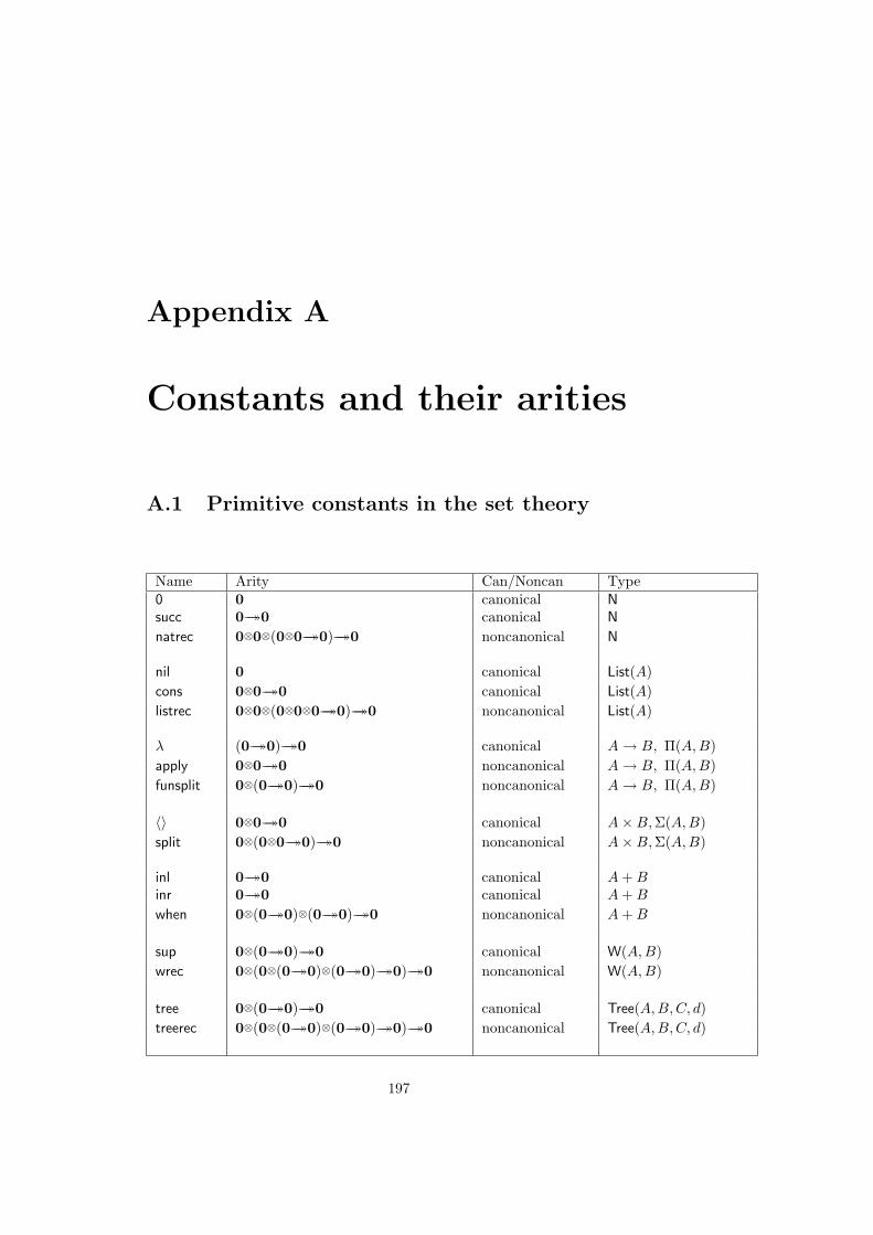
Appendix A
Constants and their arities
A.1 Primitive constants in the set theory
Name Arity Can/Noncan Type0 0 canonical Nsucc 0→→0 canonical N
natrec 0⊗0⊗(0⊗0→→0)→→0 noncanonical N
nil 0 canonical List(A)cons 0⊗0→→0 canonical List(A)listrec 0⊗0⊗(0⊗0⊗0→→0)→→0 noncanonical List(A)
λ (0→→0)→→0 canonical A → B, Π(A,B)apply 0⊗0→→0 noncanonical A → B, Π(A,B)funsplit 0⊗(0→→0)→→0 noncanonical A → B, Π(A,B)
〈〉 0⊗0→→0 canonical A×B,Σ(A,B)split 0⊗(0⊗0→→0)→→0 noncanonical A×B,Σ(A,B)
inl 0→→0 canonical A + Binr 0→→0 canonical A + B
when 0⊗(0→→0)⊗(0→→0)→→0 noncanonical A + B
sup 0⊗(0→→0)→→0 canonical W(A,B)wrec 0⊗(0⊗(0→→0)⊗(0→→0)→→0)→→0 noncanonical W(A,B)
tree 0⊗(0→→0)→→0 canonical Tree(A,B, C, d)treerec 0⊗(0⊗(0→→0)⊗(0→→0)→→0)→→0 noncanonical Tree(A,B, C, d)
197

198 APPENDIX A. CONSTANTS AND THEIR ARITIES
Name Arity Can/Noncan Typeid 0 canonical Id(A, a, b)idpeel 0⊗(0→→0)→→0 noncanonical Id(A, a, b)
{i1, . . . , in} 0 canonical U
N 0 canonical U
List 0→→0 canonical U
Id 0⊗0⊗0→→0 canonical U
+ 0⊗0→→0 canonical U
Π 0⊗(0→→0)→→0 canonical U
Σ 0⊗(0→→0)→→0 canonical U
W 0⊗(0→→0)→→0 canonical Uurec (se page 93) noncanonical U
A.2 Set constants
Name Arity{i1, . . . , in} 0N 0List 0→→0Π 0⊗(0→→0)→→0→ 0⊗0→→0Σ 0⊗(0→→0)→→0× 0⊗0→→0+ 0⊗0→→0Id 0⊗0⊗0→→0W 0⊗(0→→0)→→0Tree 0⊗(0→→0)⊗(0⊗0→→0)⊗(0⊗0⊗0→→0)→→0→→0U 0{|} 0⊗(0→→0)→→0

Appendix B
Operational semantics
The following is a formal description of the operational semantics of the poly-morphic set theory. We use the notation a ⇒ b to mean that the program acomputes to the value b. We start with programs on constructor form, whichalready are evaluated, then we continue with programs on selector form.
i1 ⇒ i1 . . . in ⇒ in
0 ⇒ 0 succ(d) ⇒ succ(d) nil ⇒ nil
cons(d, e) ⇒ cons(d, e) λ(c) ⇒λ(c) inl(d) ⇒ inl(d)
inr(e) ⇒ inr(e) 〈c, d〉 ⇒ 〈c, d〉 sup(c, d) ⇒ sup(c, d)
a ⇒ i1 b1 ⇒ q
casen(a, b1, . . . , bn) ⇒ q
a ⇒ in bn ⇒ q
casen(a, b1, . . . , bn) ⇒ q
a ⇒ 0 b ⇒ q
natrec(a, b, c) ⇒ q
a ⇒ succ(d) c(d, natrec(d, b, c)) ⇒ q
natrec(a, b, c) ⇒ q
a ⇒ nil b ⇒ q
listrec(a, b, c) ⇒ q
a ⇒ cons(d, e) c(d, e, listrec(e, b, c)) ⇒ q
listrec(a, b, c) ⇒ q
a ⇒λ(c) c(b) ⇒ q
apply(a, b) ⇒ q
a ⇒λ(c) b(c) ⇒ q
funsplit(a, b) ⇒ q
a ⇒ inl(d) b(d) ⇒ q
when(a, b, c) ⇒ q
a ⇒ inr(e) c(e) ⇒ q
when(a, b, c) ⇒ q
a ⇒〈c, d〉 b(c, d) ⇒ q
split(a, b) ⇒ q
a ⇒ sup(c, d) b(c, d, (x)wrec(d(x), b)) ⇒ q
wrec(a, b) ⇒ q
199

200 APPENDIX B. OPERATIONAL SEMANTICS
B.1 Evaluation rules for noncanonical constants
The following is an informal description of the operational semantics of typetheory. Only the rules for the selectors are given, since each expression onconstructor form is already evaluated. Let x be a variable and a, b, c, d and eexpressions of suitable arity.
Expression Computation rulecasen(a, b1, . . . , bn) 1. Evaluate a to canonical formwhere a ∈ {i1, . . . , in} 2a. If the value is of the form i1
then continue with b1
2b. If the value is of the form i2then continue with b2
. . .2u. If the value is of the form in
then continue with bn
natrec(a, b, c) 1. Evaluate a to canonical form2a. If the value is of the form 0
then continue with b2b. If the value is of the form succ(d)
then continue with c(d, natrec(d, b, c))
listrec(a, b, c) 1. Evaluate a to canonical form2a. If the value is of the form nil
then continue with b2b. If the value is of the form cons(d, e)
then continue with c(d, e, listrec(e, b, c))
apply(a, b) 1. Evaluate a to canonical form2. If the value is of the form λ(c)
then continue with c(b)
funsplit(a, b) 1. Evaluate a to canonical form2. If the value is of the form λ(c)
then continue with b(c).
split(a, b) 1. Evaluate a to canonical form2. If the value is of the form 〈c, d〉
then continue with b(c, d)

B.1. EVALUATION RULES FOR NONCANONICAL CONSTANTS 201
Expression Computation rulewhen(a, b, c) 1. Evaluate a to canonical form
2a. If the value is of the form inl(d)then continue with b(d)
2b. If the value is of the form inr(e)then continue with c(e)
wrec(a, b) 1. Evaluate a to canonical form2. If the value is of the form sup(c, d)
then continue with b(c, d, (x)wrec(d(x), b))


![· -cup]. synek - 130. FK MLADÁ BOLESLAV B: Knobloch - gt'astný. Tvrdý - wojnar (70. Sediá&ek), Scuk - synek Schubert), (46 - Bulut. FK PARDIJBICE: shejbal - Piibyl, Norek -](https://img.dokumen.tips/doc/110x75/5d574bc088c9934f278bcd99/-cup-synek-130-fk-mlada-boleslav-b-knobloch-gtastny-tvrdy-wojnar.jpg)