Pricing complex options using a simple Monte Carlo Simulation

1Copyright © SBCM 2000

Pricing complex options using a simple Monte Carlo Simulation

Among the different numerical procedures for valuing options, the Monte Carlosimulation is well suited to the construction of powerful yet simple pricing models. Itis especially useful for single variable European options where, as a result of a non-standard pay-out, a closed-form pricing formula either does not exist or is difficult toderive. In addition, the price of complex options is sometimes difficult to explainintuitively and a simulation can often provide some insight into the factors thatdetermine the pricing.

Once a basic pricing model has been constructed, it can be applied to different optionssimply by changing the pay-out function of the underlying variable to suit the particularcase. There is no further need for complicated algebraic calculations.

This article examines the performance of an extremely simple Monte Carlo simulationspreadsheet which estimates the price of options using the same assumptions and basicmethodology as the pricing models used by many banks. Although the presentation ofdetailed calculations and results is limited to LIBOR based non-standard options, theformalism is easily extended to other underlying variables such as other floating-rateindices, term swap rates and foreign exchange rates.

At the core of the simulation is an algebraic expression containing a stochastic term.This formula generates paths for the underlying variable (e.g. LIBOR, swap rate orforeign exchange rate) which are consistent with a given set of forward rates,volatilities and an assumed statistical distribution. The derivation of the generatingformula is addressed in a number of texts but the following outline emphasizes the keypoints. The model assumes that an infinitesimal process for the underlying variable S isgiven by

Sdz +Sdt = dS σµµ is the expected proportional change in S per unit time, σ is the volatility of S and dzis the Wiener process dz = ε√dt (where ε ~ N(0,1), a normal distribution of unitstandard deviation and zero mean). Using Itô’s lemma it is possible to derive theinfinitesimal process for ln(S). The resulting algebraic expression is then in a form thatcan be readily extended to finite time intervals.

For a general time interval starting at time t and ending at time T, the generatingformula for the simulated value of S at time T (ST) is

( ) ( )S = S eT t

- 12

T-t T-t2µ σ σε

+

At time T this formula generates a new value for S which depends, inter alia, on thevalue generated at time t.

The formula needs little alteration to bring in LIBOR as the specific underlyingvariable. The expected proportional change in LIBOR per unit time (µ) is given by the

Pricing complex options using a simple Monte Carlo Simulation.


logarithm of the ratio of successive values of forward LIBOR. Then the formulabecomes:

( ) ( )t-Tt-T21 -

t

Tt T

2

eLIBOR ForwardLIBOR Forward

L = Lσεσ +

×

×

(It assumes that values of implied forward LIBOR have been calculated.)

The pricing spreadsheet can now be assembled. A simple macro or procedure shouldbe written so that the spreadsheet can automatically recalculate itself for any desirednumber of runs. In a simulation of LIBOR rates, the forward LIBOR curve andresulting discount factors must first be calculated. For example, if the term is 2 yearsand the reset frequency is 6-monthly, 4 discount factors and 4 values of 6 monthLIBOR will be relevant to the pricing of transactions (For spot starting transactionsthere are only 3 relevant discount factors and values of LIBOR).

While it is recognized that this specification of the LIBOR process, using staticdiscount factors, is not arbitrage-free, the results have proved accurate for a widerange of product types.

If the particular spreadsheet (e.g. Lotus 1-2-3 or Excel) does not provide a function forcalculating random normal deviates but does provide a function which generatesnumbers from a uniform distribution over [0,1], the following approximation for anormal deviate ε can be used

( )ε ~ N 0,1 R - 6ii=1

i=12

≈ ∑ To standardize the model so that a minimum number of changes is needed to pricedifferent options, it is useful to represent the option cash flows as though they werepart of an interest rate swap. Another reason for this is that many of the options thatwe price at SBCM are typically embedded in structured notes and we price the swapwhich enables the issuer of the note to swap into a conventional floating rate liability.So each option is split into a LIBOR leg that is received and a constrained LIBOR legthat is paid, where the constraints reflect the desired optionality. The received LIBORis the simulated LIBOR generated by the formula and the constrained LIBOR leg is thesimulated LIBOR leg modified by the inclusion of IF, MAX or MIN statements asappropriate.

Hence, for each simulation run, values are assigned to both legs of the swap in everyperiod. By calculating the net present value (NPV) of the difference between the swaplegs using the per-period discount factors and repeating the exercise for severalthousand simulation runs, a distribution of NPVs can be constructed. The mean of thisdistribution is identified as the up-front premium (or the net premium when more thanone embedded option is implied).



To illustrate this method, it is shown below how to estimate the price of two products:

One-way (“sticky”) floating rate note.

This is a floating rate note (FRN) whose coupon cannot fall below its previous settingor rise by more than a pre-defined amount between consecutive periods. A buyer ofsuch a note has bought a floor and sold a cap. The floor rate is equal to theimmediately preceding coupon setting. The cap rate is equal to the sum of theimmediately preceding coupon setting and the maximum per-period increment.Clearly, the cap and floor rates will vary with the actual coupon settings that occurduring the life of the note. Hence the options are said to be path dependent.

The example chosen is a 2 year DEM 6 month LIBOR one-way FRN with a maximumper-period increment of 0.25%. The coupon is 6 month DEM LIBOR flat and eachsuccessive coupon setting is never less than the previous setting. However, eachsuccessive coupon setting cannot exceed the previous coupon by more than 0.25%.The caps and floors implicit in this structure can be priced using the simulation to givean expected up-front premium.

This type of structure often requires that the price be given in terms of the coupon’smargin over LIBOR. This is easily calculated from the up-front premium by dividing itby the sum of the discount factors [(see table)] and multiplying the result by thecoupon frequency (i.e. for semi-annual coupons, multiply by 2).

Spot and Receive PaySemi-annualDiscountForward 6 mth UnconstrainedConstrained PV of

Period Factor DEM LIBOR Volatility N(0,1) LIBOR L1 LIBOR L2 cash flow0 1.0000 4.490% 20.00% (0.433)1 0.9773 4.615% 20.00% (1.041) 4.49% 4.49% 0.00%2 0.9550 5.254% 20.00% 1.462 3.94% 4.49% -0.26%3 0.9303 5.696% 20.00% 0.696 5.47% 4.74% 0.34%4 0.9044 6.271% 20.00% 0.478 6.47% 4.99% 0.68%

=====NPV = 0.76%

=====

( )( )L2 = L1L2 = M IN MAX L1 L2 , L2 for j = 1, 2 or 3

(Where L2 is the co nstrained LIBOR coup on set at time j and L1is the unconstrained LIBOR also set at the beginning of period j)

Equivalent semi - annual margin over L IBOR =2 NPV

360365

Discount F actor at P eriod t

0 0

j j j-1 j-1

j j

t=1

t =4

, .+

× ×

∑

0 25%

A Black, Derman and Toy (BDT) model using a single volatility of 20% gives an up-front premium value of 0.587%. Figure 1 shows the distribution of NPVs given by theMonte Carlo simulation after 8,000 runs



Distribution of Simulated NPV(Maximum Coupon Increase Per Period = 0.25%. Coupon Cannot Decrease.)

0.00

0.05

0.10

0.15

0.20

0.25

0.30

0.35

0.40

0.45

-3% -2% -1% 0% 1% 2% 3% 4% 5% 6% 7% 8% 9%

Simulated NPV

Rel

ativ

e Fr

eque

ncy

BDT Model Premium = 0.587%Average Simulated NPV = 0.583%Median NPV = 0.401%Maximum NPV = 8.327%Minimum NPV = -2.852%Standard Deviation = 1.132%Standard Error = 0.013%Number of simulation runs = 8,000

Single date knock-out cap.

The knock-out cap is designed to reduce the up-front premium payable by the optionbuyer. The knock-out rate is higher than the cap rate and whenever LIBOR sets belowthe knock-out rate, a knock-out cap is indistinguishable from a conventional cap.When LIBOR sets above the knock-out rate, the cap ceases to operate.

Two features of a knock-out structure must be distinguished. First, the knock-outcondition can apply on one or several dates. Second, if a knock-out occurs, it caneither be for that period only or it can apply to all of the remaining caplets. From apricing point of view, the simplest case is a per-period knock-out where the conditionis applied in each period but only to the caplet for that period. In this case the buyer ofsuch a cap has effectively bought a regular cap at the cap rate and has also sold aregular cap and a binary cap, both at the knock-out rate. The binary pay-out is equalto the difference between the knock-out rate and the underlying cap rate.

The example chosen here is more difficult to price. It is a 3 year GBP 6 month LIBOR8% cap with a knock-out rate of 10% applicable after 1 year. While the knock-outcondition is applied on only one date, if the condition is satisfied, all of the remainingcaplets vanish. This type of knock-out cap is not equivalent to a combination ofconventional and binary caps. As far as the simulation goes, it is not difficult to adaptthe model. In each run a flag is set up to monitor the level of LIBOR on the knock-outdate. Whenever the knock-out rate is breached, the constrained LIBOR leg of theswap in all subsequent periods is set equal to the unconstrained LIBOR leg, i.e. allremaining caplets vanish. The simulation is run as before. Using the same notation asin the previous example, the constraint equation is given by:

L20 = L10

L21 = MIN(L11 , 0.08)FLAG: IF(L12 > 0.1, 0, 1)



L2j = IF(FLAG = 0, L1j , MIN(L1j , 0.08)) for j = 2, 3, 4 or 5

A volatility of 20% is assumed. A closed-form solution pricing model using a singlevolatility of 20% gives an up-front premium of 1.11%. The resulting distribution ofthe NPV from the simulation is given in figure 2.

Distribution of Simulated NPV(Cap Strike = 8%, Knock-out Rate = 10%)

0.0

0.1

0.2

0.3

0.4

0.5

0.6

0.7

0.8

0.5% 1.5% 2.5% 3.5% 4.5% 5.5% 6.5% 7.5% 8.5% 9.5% 10.5% 11.5% 12.5% 13.5%

Simulated NPV

Rel

ativ

e Fr

eque

ncy

Calculated Premium = 1.11%Average Simulated NPV = 1.11%Median NPV = 3.48%Maximum NPV = 12.18%Minimum NPV = 0%Standard Deviation = 1.67%Standard Error = 0.02%Number of simulation runs = 8,000

The simulation model is easily changed to price both a multi-date knock-out where allof the remaining caplets disappear if the knock-out level is breached and a per-periodknock-out. The premia are 0.43% and 0.49% respectively.

The sensitivity of the option price to changes in the level of interest rates andvolatilities can be calculated from the simple model. Essentially 2 parallel simulationsare run. For example, the vega of an option is estimated by running a simulation at theoriginal volatility and simultaneously running a simulation at a volatility 1% higher butusing the same set of normal deviates. Similarly, the delta would be estimated byadjusting the forward LIBOR rates upward by 1 basis point and running 2 parallelsimulations for the original and shifted forward curves. Using the simulation for aconventional 3 year GBP cap at 10% gives a delta of 0.41 and a vega of 5.3 (a Blackmodel calculation gives 0.41 and 5.6). For very small values of vega, of the order of 1basis point, the simple model used here may be inaccurate owing to the sampling error.

While the aim of this article has been to present as simple a model as possible, theaccuracy of the model can be improved without any major increase in complexity.Since the estimate of the option value is a sample mean from an underlyingdistribution, some variation will be observed between sets of simulations. Thestandard deviation of the sample means (the standard error) scales inversely with the



square root of the number of runs, i.e. quadrupling the number of runs will only doublethe accuracy but will proportionately increase the running time. A better method forreducing the standard error is to use antithetic variables. This relies on the fact thatany finite normal deviate ε has the same probability of being drawn from a N(0,1)distribution as -ε.

The method then requires that two parallel simulations are run for normal deviates ±ε.This produces 2 distributions of NPVs and the arithmetic mean of the means of thedistributions should then be a more reliable estimate of the option value.

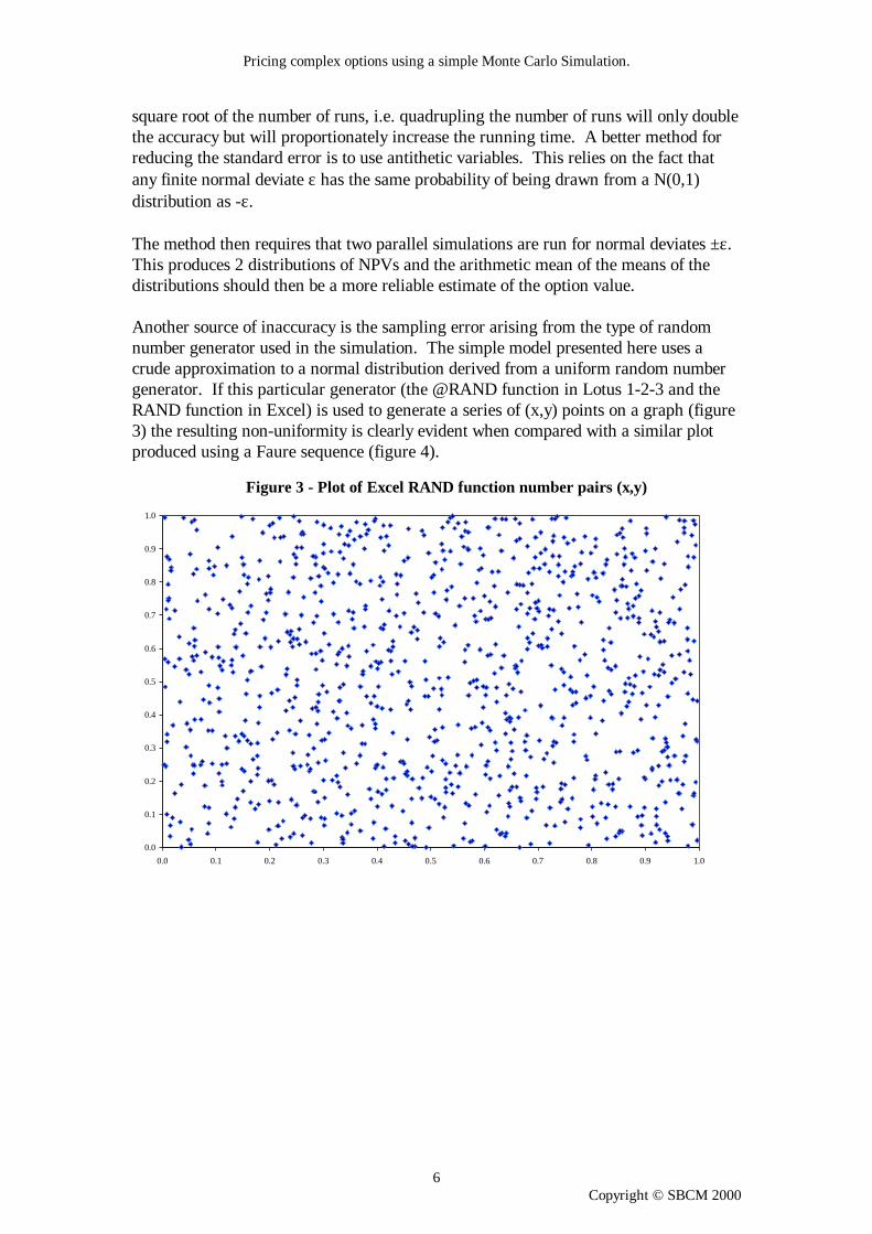
Another source of inaccuracy is the sampling error arising from the type of randomnumber generator used in the simulation. The simple model presented here uses acrude approximation to a normal distribution derived from a uniform random numbergenerator. If this particular generator (the @RAND function in Lotus 1-2-3 and theRAND function in Excel) is used to generate a series of (x,y) points on a graph (figure3) the resulting non-uniformity is clearly evident when compared with a similar plotproduced using a Faure sequence (figure 4).

Figure 3 - Plot of Excel RAND function number pairs (x,y)

0.0

0.1

0.2

0.3

0.4

0.5

0.6

0.7

0.8

0.9

1.0

0.0 0.1 0.2 0.3 0.4 0.5 0.6 0.7 0.8 0.9 1.0



Figure 4 - Plot of Faure sequence number pairs (x,y)

0.0

0.1

0.2

0.3

0.4

0.5

0.6

0.7

0.8

0.9

1.0

0.0 0.1 0.2 0.3 0.4 0.5 0.6 0.7 0.8 0.9 1.0

A number of articles in financial publications demonstrated the greater accuracy ofFaure and Sobol sequences over the more conventional methods used for lowdimension simulations, (e.g. RISK June 1996, pages 63-65). However, such methodswould increase the complexity of the model here, against the aim of this article topresent the simplest possible model which reproduces the results of larger and morecomplicated calculations. n

Peter Fink is senior vice president and head of marketing at SMBC CapitalMarkets, Inc., New Yorke-mail: [email protected]

Documents

Pricing complex options using a simple Monte Carlo Simulation