Embed Size (px)
Citation preview

A Monte Carlo Method for Pricing American
Options
by
LAM Wing Shan
Thesis
Submitted to the Faculty of the Graduate School of
The Chinese University of Hong Kong
(Division of Mathematics)
In partial fulfillment of the requirements
for the Degree of
Master of Philosophy
August, 2003
The Chinese University of Hong Kong holds the copyright of this thesis. Any
person(s) intending to use a part or whole of the materials in the thesis in a
proposed publication must seek copyright release from the Dean of the Graduate
School.

f会/ uisy3A_一 ..
ti ——^^^ 一 V || m 旧 Y 61 i
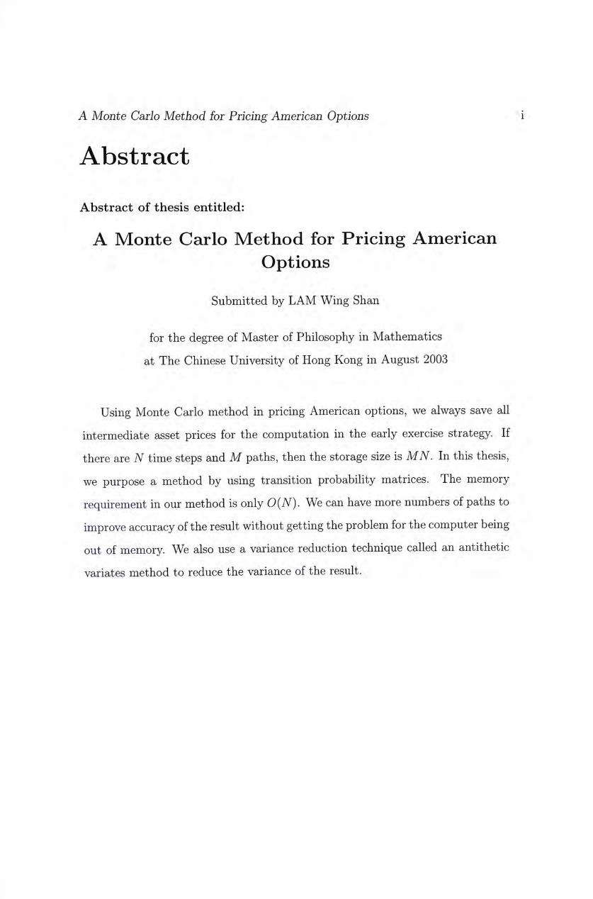
A Monte Carlo Method for Pricing American Options i
Abstract Abstract of thesis entitled:
A Monte Carlo Method for Pricing American Options
Submitted by LAM Wing Shan
for the degree of Master of Philosophy in Mathematics
at The Chinese University of Hong Kong in August 2003
Using Monte Carlo method in pricing American options, we always save all
intermediate asset prices for the computation in the early exercise strategy�If
there are N time steps and M paths, then the storage size is MN. In this thesis,
we purpose a method by using transition probability matrices. The memory
requirement in our method is only 0{N). We can have more numbers of paths to
improve accuracy of the result without getting the problem for the computer being
out of memory. We also use a variance reduction technique called an antithetic
variates method to reduce the variance of the result.

ii
i-i—^ 二趟亜
豕干寸卞維法示口夫式期 f e疋 1貝
當使用蒙特卡羅法來計算美式期權時,我們往往把所有的價格儲存起
來。如果有N個間距及M條路徑,那麼MN便是儲存的容量了。在
這篇論文中,我們會使用機率矩陣來改變儲存的容量爲0(N),因此對
於電腦記憶、容量的限制,我們依然能夠使用足夠數目的M來得到準確
的結果。此外,我們會使用antithetic variates方法來減少結果的方差。

A Monte Carlo Method for Pricing American Options iii
ACKNOWLEDGMENTS
I wish to express my deepest gratitude to my supervisor Dr. Kit-Ming Yeung
for his valuable advice, kind supervision and constant encouragement throughout
the period of my postgraduate study. This work have not been possible without
the support and help of him. Also, special thanks my colleagues M.P. Chau, C.Y.
Ho, P.T. Ho, K.T. Hung and C.Y. Wong for their many helpful discussions.

Contents
1 Introduction 1
2 Background on Option Pricing 3
2.1 Financial options 3
2.1.1 Basic terms of options 3
2.1.2 Trading strategies 4
2.1.3 The Principle of no Arbitrage 5
2.1.4 Rational boundaries on Option Prices 5
2.1.5 American Options 6
2.1.6 Put-Call Parity 7
2.2 Black-Scholes equation 8
2.2.1 Derivation of Black-Scholes equation 8
2.2.2 Solution to the Black-Scholes equation . . . . 10
3 Review on Monte Carlo Method 15
3.1 Monte Carlo Simulation 15
3.2 Pricing an option using Monte Carlo Method 18
3.3 Antithetic Variates Method 21
iv

A Monte Carlo Method for Pricing American Options v
4 Cell Partition Method 23
4.1 An Advantage of the Cell Partition Method 23
4.2 The Algorithm 24
5 Numerical Results 35
6 Conclusion 39
Bibliography 41

Chapter 1
Introduction
Increasingly complex and sophisticated financial products continue to be intro-
duced and accepted in the marketplace. The Monte Carlo method is a useful tool
for pricing American-style options, i.e., where the owner has the right to exercise
early. However, a major difficulty in valuing American-style options is the need
to estimate optimal exercise policies as well. Standard simulation procedures are
forward algorithms , i.e., paths of state variables are simulated forward in time.
Given a state trajectory and a pre-specified exercise policy, a path price is de-
termined. An average over independent samples of path prices gives an unbiased
estimate of the options price. By contrast, pricing procedures for assets with
early-exercise features are generally backward algorithms. That is the optimal
exercise strategy at the maturity of the contract is easily determined. Proceed-
ing backwards in time, the optimal exercise strategy and corresponding price are
determined by dynamic programming. The problem of using simulation to price
American options stems from the difficulty of applying an inherently forward-
based procedure to a problem that requires a backward procedure to solve.
In this thesis, we use transition probability matrices for pricing an American
option. More precisely, we use a grid to partition the time and the payoff into
numbers of cell. The hope is that, we can reduce the error of our result without
1

A Monte Carlo Method for Pricing American Options 2
increasing the memory.
The thesis is organized as follows. A little background on options is provided
in chapter 2. We will give some review on the Monte Carlo method in chapter 3.
In chapter 4, we introduce our approach called cell partition method to price the
American options. In chapter 5, we will give some numerical results to illustrate
the result by our method. Finally, chapter 6 summarizes the thesis.

Chapter 2
Background on Option Pricing
Options have been around for many years, but they were first traded in an or-
ganized exchanged on 26th April 1973 [3, 5, 7]. The Chicago Board Options
Exchange(CBOE) is the first to standardize the listed options. And put options
were introduced in 1977.
2.1 Financial options
2.1.1 Basic terms of options
We first discuss the definition and meaning of different terms in option trading.
An option is a contract between two parties that gives one party the right to buy
or sell a specific amount of an underlying asset to the other party at a specific
price on or before some specific dates. The price at which the underlying asset
is traded is called the exercise price or strike price. The specific date when the
option is no longer valid is the expiration date. The price of an option is referred
to as its premium. If an option can only be exercised on the expiration date,
then the option is called a European option, while if the exercise is allowed on
or before the expiration date, then it is called an American option. The option
holder is the party who buys the right, the option writer is the party who sells
3

A Monte Carlo Method for Pricing American Options 4
the right. A call option gives the right to buy the underlying asset. A put option
gives the right to sell the underlying asset. The holder of a call option wants the
stock price to be above the strike price. The holder and the writer are said to be
in the long and short positions of the option contract, respectively.
In the option pricing theory, there is no arbitrage opportunities, which is
called the no-arbitrage principle. We will give more details in the section (2.1.3).
2.1.2 Trading strategies
Consider a European call option on an underlying asset S(t),where t is the current
time. The expiration date of the option is T and the exercise price is K. If
S{T)�K, then the holder of the call option will choose to exercise the option
because he can buy the asset, which is worth S{T), at the price K. Therefore,
the holder gain S{T) 一 K, However, if S{T) < K, then the holder will forfeit the
right to exercise the option since he can buy the underlying asset in the market
at a price less than the strike price K. The terminal payoff of a European call is
C{S,T) = max(S{T)-K, 0)
The payoff is also the value of the call option at the expiration date. We can
plot the payoff as a function of the underlying asset is known as a payoff diagram.
We illustrate this in the following figure.
0 K S(IJ

A Monte Carlo Method for Pricing American Options 5
Similarly, the terminal payoff of a European put is
F(S,T)=m^x(K-S(T),0)
The payoff diagram is
0 K S(J)
2.1.3 The Principle of no Arbitrage
This principle is also called the law of one price. It states that two equivalent
goods in the same competitive market must have the same price.
The no arbitrage principle can be easily seen to hold in an efficient market.
For example, if we assume that two equivalent derivatives A and B are at $59
and $61, respectively. Assume that there is no transaction cost, a trader can
get a riskless profit of $2 by buying derivative A and selling derivative B. The
trader who engages in such transactions is called an arbitrageur. In an efficient
market, this will be a very short period of time as all the participants are aware
of arbitrage opportunities when they arise.
2.1.4 Rational boundaries on Option Prices
Call options give the holder the right to buy a stock. If the value of a call option
is greater than the current price of the stock, Sq, where So = 5(0), then there is
an arbitrage opportunity. The reason is that a writer of the call option can make
a riskless profit by selling a European call option for C, where C is the value of

A Monte Carlo Method for Pricing American Options 6
the European call option on the stock, or an American call option for Ca, where
Ca is the value of the American call option on the stock, and buy the stock for Sq.
That is she makes C - Sq or Ca - Sq, TO avoid arbitrage opportunities happen,
we have the rational boundaries:
C < SQ , CA < SQ
Similarly, the upper bounds for put options:
P<K , Pa <K
where P is the value of a European put option; and Pa is a value of an American
put option.
By using the no arbitrage argument, we get a better upper boundary for a Euro-
pean put:
P < Ke八T-t)
where r is the risk-free rate, t is the current time and T is the expiration date
of the stock. If not, we suppose P > then an arbitrageur can sell a
European put for P and put it in the bank. At the expiration date T, she gets a
riskless profit P > Kd"�T-t"> from the bank. Using an arbitrarge principle again,
we can get a better lower boundary for a European put:
P > Ker(T-t) — s
2.1.5 American Options
American options give more rights than their European equivalent and are there-
fore more valuable, that is
Ca>C , PA >P

A Monte Carlo Method for Pricing American Options 7
We would not exercise an American call option early. The reason is that, for
an American call option, we have the inequality
CA>S-K
If the holder exercise the option early, then she would pay for a stock with
Ca + K � S
At the expiration date T, her payoff is
S(T) - {Ca + K) < max(5(T) — K, 0)
Therefore, early exercising an American call option would decrease the profit
of the holder.
For all types of options, we have
value of option = intrinsic value + time value
For example, if the underlying asset is trading at $75, a call option with a strike
price $70 will have $5 of intrinsic value. The reason is that the call owner has
the right to buy the stock for $70. For a put option with that strike price has no
intrinsic value because it does not make sense to sell a stock for $70 when it can
be sold for $75. An option is said to be in the money if it has positive intrinsic
value, out of the money if it has zero intrinsic value, and at the money if the
strike price is equal to the spot price of the stock.
2.1.6 Put-Call Parity
Put-call parity states the relation between the prices of calls and puts. To illus-
trate the claim, we compare the values of two portfolios, A and B, formed at the
present time t.
Portfolio A consists of a European call on a non-dividend paying asset with the

A Monte Carlo Method for Pricing American Options 8
Asset value at expiration date S(T) < X S{T) > X
Portfolio A K S(T)
Portfolio B K S{T)
Table 2.1: Payoff at expiration date of Portfolios A and B.
strike price K and the expiration date T. And Ke<T~t�dollars in the bank.
Portfolio B consists of one share of stock and a European put with the strike
price K and the expiration date T.
Table 2.1 lists the payoff at expiration date of the two portfolios for the two cases:
S{T) < and S(T) > X. The values of the two portfolios at the expiration
date T are the same. Due to the no arbitrage principle, the values of the two
portfolios must be the same at the current time, that is
C + Ke'^^-'^ = P ^ S (2.1)
2.2 Black-Scholes equation
In 1973, Fischer Black and Myron Scholes made an enormous contribution to the
theory of finance by deriving a formula to price European call options on non
dividend paying assets. Many traders and investors now use the formula to value
stock options in markets throughout the world.
2.2.1 Derivation of Black-Scholes equation
Assume the evolution of the price of a non dividend paying asset S follows the
geometric Brownain motion:
号=rdt + adZ, (2.2) U

A Monte Carlo Method for Pricing American Options 9
where r is risk-free interest rate; a is the volatility of the stock; and dZ is the
standard Wiener process, which satisfies a normal distribution N{0, And
E{{dZf) = dt , Y8.i{{dZf) = o{dt).
Assume terms of order o{dt) as essentially zero, then (dZ)? = dt and hence
{dSf 二 (J^S'^dt. (2.3)
The value of an option, denoted by V, is a function of the current value of the
underlying asset S, and the time t: V = V{S, t). Using Ito's lemma,
and by (2.2) and (2.3), we have
We consider the value of a portfolio of one long option position and a short
position in some quantity A of the underlying asset:
U = V{S,t)-AS.
The value of the portfolio changes from the time t to t + dt:
tm 二 dV - AdS
if we choose
A 抓 八=液’
then the randomness is reduced to zero.

A Monte Carlo Method for Pricing American Options 10
Thus the portfolio that changes by
is completely riskless. If we have a completely risk-free change dH in the portfolio
value n, then it must be the same as the growth we would get the equivalent
amount of cash in a risk-free interest rate in bank. By the no arbitrage principle,
we have
dU = rUdt. (2.5)
Substituting (2.4) into (2.5), we find that / dv\
dn 二 - rS— dt. V 肪乂
Then we have the following equation:
= 0. (2.6)
This is the Black-Scholes partial differential equation.
2.2.2 Solution to the Black-Scholes equation
Consider the value of a non dividend paying European call C{S, t) that satisfies
(2.6) and final condition, that is dC 1 � d c ^ �
i + (2,7) [C{S, T) = max(5 - K, 0)
where T is the expiration date of the underlying asset. Applying the transforma-
tion
5 = S'e-r�T-t�,c = C'e-八T-t) , c' = C'{S'A).
to equations (2.7). we get a new set of equations 1 多'
1 + (2 ,8)
�C\S',T) = m a x ( 5 ' - A ' , 0 ) .

A Monte Carlo Method for Pricing American Options 11
Applying another transformation to equation (2.8),
S' = Ke'^+i''"^ ,T = T - t , C\S', t) = KV{x, r).
We get
‘^ _ 1 2 种
< ~ ^二 5 � ( 2 . 9 )
This is the well-known heat equation, satisfying
< ~ ^二? (2.10) � Q{x,0) = (j){x - Xq),
with a solution to (2.10) with any fixed xq and any initial datum cj).
1 ( 工 - 工 0 ) 2
Q{x,t;xo) = - j = = e 认 .
Therefore, the solution to (2.9) is roo
V{x, T) 二 max(e^° - 1, 0)Q{x, r; xo)dxo J oo
POO = / (e卯—1, 0)Q{x, r; Xo)dxo
Jo 广 1 (卜邮)2
Jo V2a^7Tr . 1 (工-〜2 fOO I (…0)2
= / 一 - P ^ ^ ^ d X Q - / e dXQ Jo V^a'^nr Jo V2a^7rT
二 / 1 + /2,
where
广 1 (工-工。)2 ^
I i = e 恥 e i ^ c b o , Jo V2a'^7TT 广 1 (X-xq)
I2 = e dxo. Jo w2(t'^ttt

A Monte Carlo Method for Pricing American Options 12
We find Ii and I2.
, r 1 (工-工,0)2 J 12= , - e dxo
Jo V2a^7TT 1 r—00 对2 工_工0
— — / e—“^dyi , by substituting yi 二 ^ V27r J-2- cryY
CRY/R
where N(.) is the cumulative standard normal distribution.
广. 1 (卜
11 = / e 帅 e ~ - ^ d x o Jo V^a'^TTT 1 厂⑴ 1
v27r Jo cryV 1 厂⑴ 1
一 V^ Jo 4 1 厂⑵ 1 =——=e / ——^e dxo
V^ Jo cry^ 1 � , , {x + a � ) 一 Xq = e 2 dy2 , by letting y2 = — �
= 叫 禱
Therefore the solution to (2.9) is
The solution to (2.8) is
(log* + ia2(T -t)\ 丁, M (log 安-\<j\T-t)\ C'[S',t) 二 S'N Uk _L -KN 'k 2V __)_ \ (jyT -1 y 乂 oML -1 y
And the solution to the origin equation (2.7) is
c m 二 s 4 i � g• 作 ; ^ � T — t ) � � f - ( r ; i ^ ) ( " ) ) 乂 cta/T^— 力 y 乂 av-t —t y
二 SN{di)-Ke-八 T-t�N胸,

A Monte Carlo Method for Pricing American Options 13
where
务 + ( ⑵ ( 了 - 力 ) . ( 2 . 1 2 )
For a non dividend paying European put P{S, t) which satisfies:
( d P 1 dP ^ ^ 1 + 5 改 蔽 竹 ^ 液 - 《 二 0 , (2.13)
I P(5',T) = max(K-5 ' , 0).
The solution to (2.13) is easily to derived by using the value of a European call
and put-call parity that stated in (2.1).
P - C + 一 s
where di and d] are given by (2.11) and (2.12) respectively and
However, we cannot apply this equation directly to determine the price of an
American option. The Black-Scholes equation for a European put cannot give
the correct price for an American put, so we need find other methods to solve
it. How to price an American option? There are several methods to deal with
this problem. For example, Cox, Ross and Rubinstein (1979) [5] use the CRR
model to price an American option. The basic idea is to approximate on an
appropriately chosen finite state Markov chain which converges in distribution
to the continuous-time process of interest, then we get the approximate option
value by maximizing over all possible early exercise strategies of the corresponding
present values by backward algorithms. However, it is impossible if the dimension
of the problem is higher than 3 since the computing time grows exponentially in
the number of state variables. Boyle (1979) introduced a simulation method
A Monte Carlo Method for Pricing American Options 14
which is known as the Monte Carlo method. A main advantage of the Monte
Carlo method is that computational time grows linearly with the number of state
variables and is able to approximate high dimensional probability measures. We
will have a brief overview on Monte Carlo method in the next chapter.

Chapter 3
Review on Monte Carlo Method
In recent years, the complexity of numerical computation in financial theory and
practice has increased enormously. We demand more in computational speed
and efficiency. Numerical methods are used for a variety of financial purposes.
The Monte Carlo method is a useful tool for these calculations. The Monte Carlo
method is used to simulate the asset price paths and use it to compute the optimal
exercise strategy for pricing an option.
In this chapter, we compute the price of an option using Monte Carlo Method.
We also describe its advantages and disadvantages and discuss the technique to
improve the efficiency of the method which is based on the idea of P. Boyle [4 .
3.1 Monte Carlo Simulation
Generally, Monte Carlo method can be viewed as a branch of experimental math-
ematics in which one uses random numbers to conduct experiments. Although it
is useful for doing statistical experiments, the randomness of its sampling means
that it will over-sample and under-sample from various parts of the distribu-
tion's shape unless a very large number of simulations are performed. Consider
the problem of approximating the integral f{x)dx with an integration domain
15
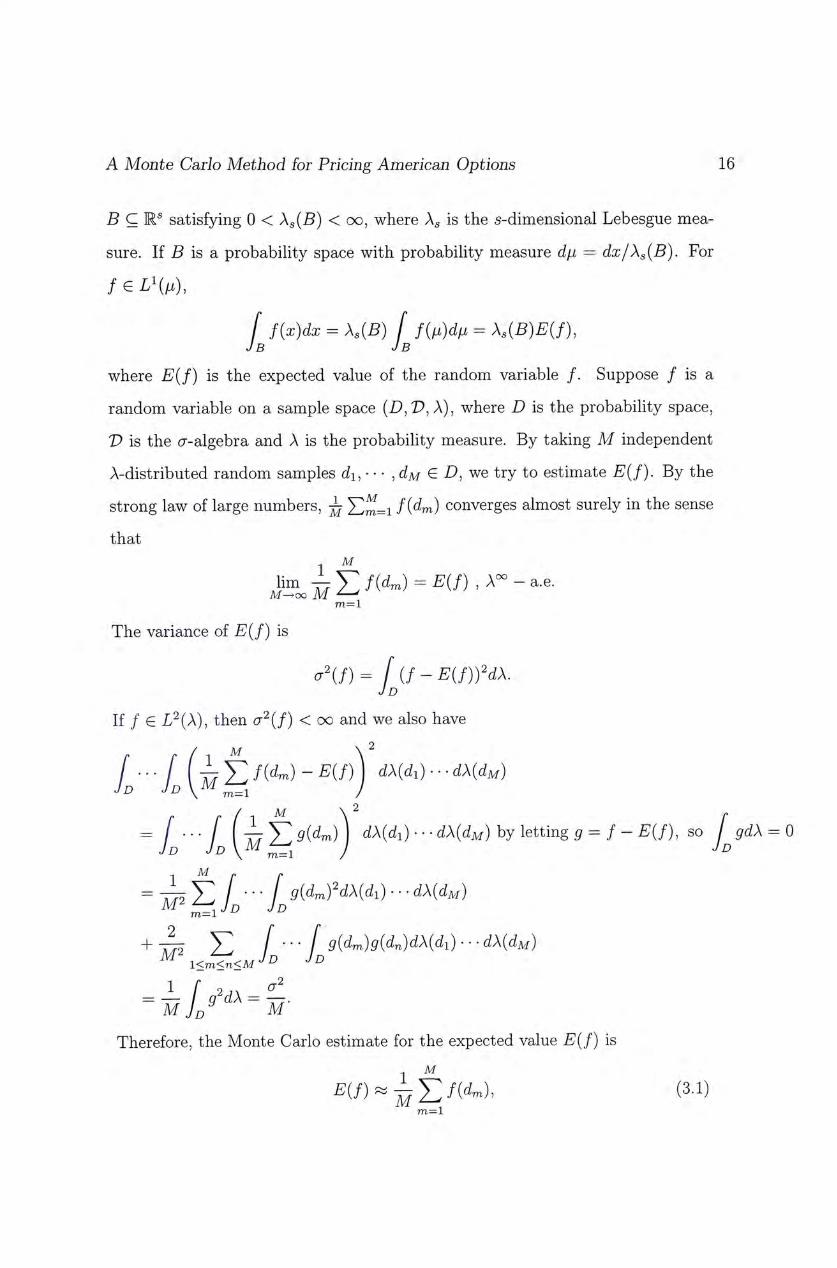
A Monte Carlo Method for Pricing American Options 16
B CR^ satisfying 0 < As(5) < oo, where Ag is the 5-dimensional Lebesgue mea-
sure. If B is a probability space with probability measure d[i 二 dx/\(^B�. For
/ “ 1 ( " ) ,
[f{x)dx = Xs{B) [ f{^)dfi = Xs{B)E{f), JB J B
where E(f) is the expected value of the random variable f. Suppose / is a
random variable on a sample space (D,T>, A), where D is the probability space,
V is the cr-algebra and A is the probability measure. By taking M independent
A-distributed random samples di, • • • ,dM ^ D, we try to estimate E{f). By the
strong law of large numbers,吾 fi^m) converges almost surely in the sense
that 1 M
lim - Y^ f{dm) = E{f) , A � - a . e . M^oo M ^‘ m=l
The variance of E{f) is
一(/)= [ if - E{f)fdX. JD
If / G 1/2(A), then cr^(/) < oo and we also have
r r / 1 M � 2 / … 去;E f{dm) - E{f) dX{d,) . . . dX{dM)
Jd Jd y^-^ /
= [ … . [ l ^ y g i d m ) ] by letting 5 = /-五(/), so [ gdX = 0 Jd JD V^f^i J 九
1 M r r
^ Jd JD
+ ^ […g{dm)9{dn)dX{di)... dX(dM) ^ IK^ukmJd JD
m A ) m Therefore, the Monte Carlo estimate for the expected value E{f) is
M
m—1
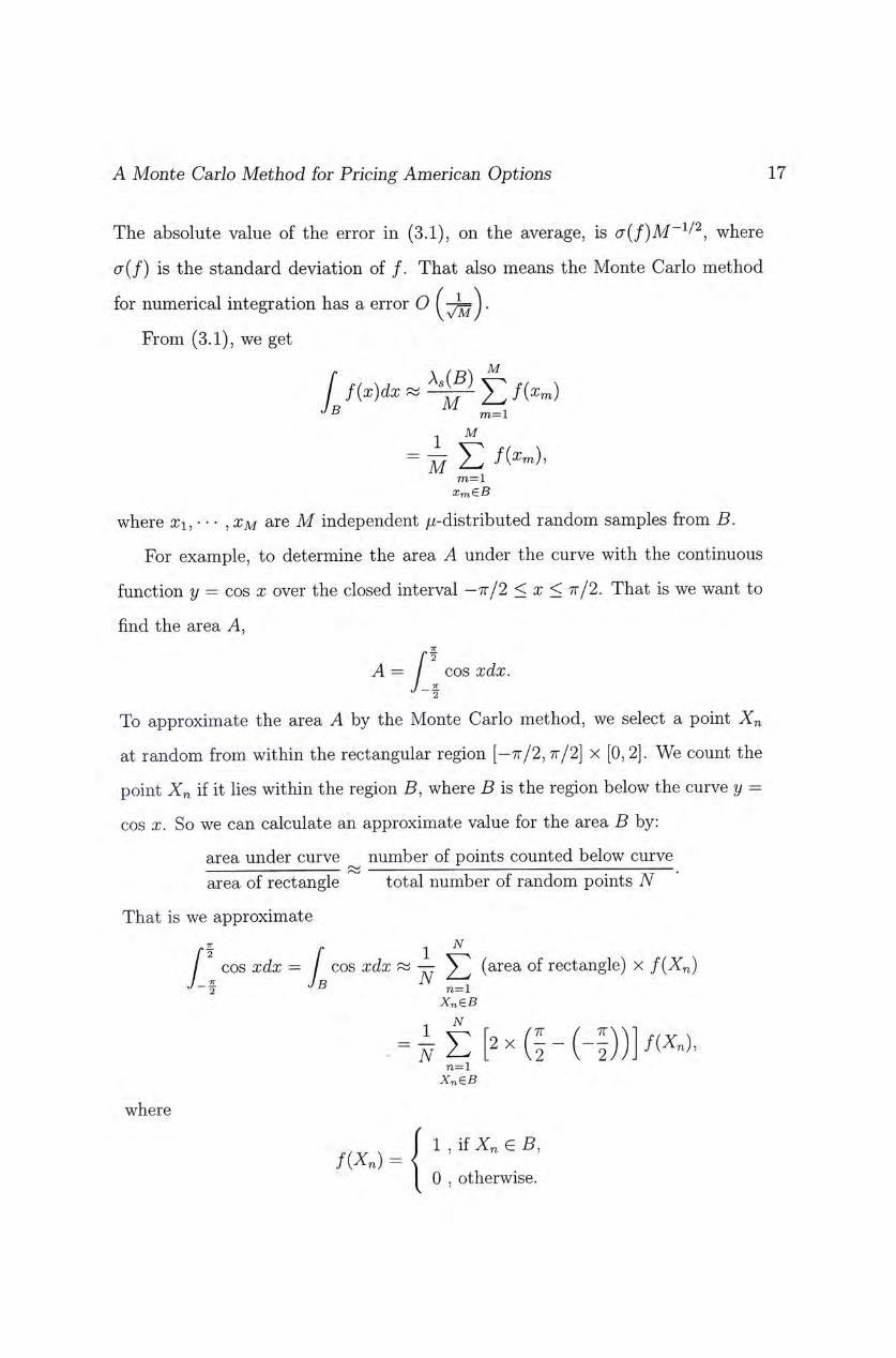
A Monte Carlo Method for Pricing American Options 17
The absolute value of the error in (3.1), on the average, is where
a ( / ) is the standard deviation of / . That also means the Monte Carlo method / 1 \
for numerical integration has a error O ^ .
From (3.1), we get
[mdx f M
1 M E / � ’ m=l Xm^B
where Xi, • • •,Xm are M independent ^-distributed random samples from B.
For example, to determine the area A under the curve with the continuous
function y = cos x over the closed interval -7r/2 < x < 7r/2. That is we want to
find the area A,
A = cos xdx.
To approximate the area A by the Monte Carlo method, we select a point Xn
at random from within the rectangular region [—7r/2, 7r/2] x [0, 2]. We count the
point Xn if it lies within the region B, where B is the region below the curve y =
cos X. So we can calculate an approximate value for the area B by:
area under curve � 皿 m b e r of points counted below curve area of rectangle total number of random points N
That is we approximate .f r Y N / COS xdx 二 / cos xdx ^ — ^ (area of rectangle) x f(Xn)
Jb N n二 1 XneB
卿, n=l
XneB
where
1 , if Xn G /⑷二
I 0 , otherwise.
A Monte Carlo Method for Pricing American Options 18
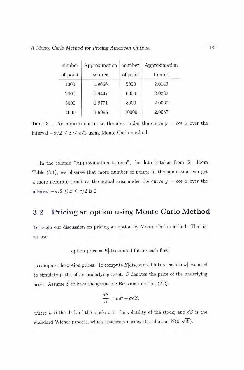
number Approximation number Approximation
of point to area of point to area
1000 1.9666 5000 2.0143
2000 1.9447 6000 2.0232
3000 1.9771 8000 2.0067
4000 1.9996 10000 2.0087
Table 3.1: An approximation to the area under the curve y = cos x over the
interval -7r/2 < x < 7r/2 using Monte Carlo method.
In the column "Approximation to area", the data is taken from [6]. From
Table (3.1), we observe that more number of points in the simulation can get
a more accurate result as the actual area under the curve y = cos x over the
interval -7r/2 < x < 7r/2 is 2.
3.2 Pricing an option using Monte Carlo Method
To begin our discussion on pricing an option by Monte Carlo method. That is,
we use
option price = E'[discounted future cash flow
to compute the option prices. To compute E[discounted future cash flow],we need
to simulate paths of an underlying asset. S denotes the price of the underlying
asset. Assume S follows the geometric Brownian motion (2.2):
dS 7, -—=(idt + adZ, o
where ji is the drift of the stock; a is the volatility of the stock; and dZ is the
standard Wiener process, which satisfies a normal distribution iV(0,Vdi),

A Monte Carlo Method for Pricing American Options 19
If there are M simulations and N time steps between the current time to
and the expiration date T with to < h < . . . < t^ = T, where tj =力o + j M ,
1 < j < we have
A T — to A 力 = 了 .
The known current asset price is S^{to) = Sq, 1 < i < M, and there is a risk-free
rate r. The z-th price path is defined by
S] = 1 < i < M , 1 < j < TV (3.2)
where S'j = S\tj) is the asset price on the z-th path at time tj with SQ = So,
1 < i < M; and ej are independent, identically distributed, standard normal
random numbers.
Now, we introduce transition probability density PtriS) for S, which satisfies
the condition (2.2), with
r Ptr{S)dS=l J —oo
and ptr{S) satisfies the backward Kolmogorov equation
警 +臺〜禁智 = 0 . (3.3) For a terminal payoff f[S), we define E[f{S)] is the expected value of the function
m , then
E[f{S)] 二�f{S)pUS)dS. (3.4) J —OO
Suppose E[/(5T)] is the solution of the function ptr{S, T) at time T, we have
pUS,T) = E[f{ST)].
If E[f{ST)] represents the amount of money received at time T and the current
time is to, let
Vl^S^to) 二 e—邓—t�tr� t).

A Monte Carlo Method for Pricing American Options 20
We substitute
into (3.3). We see that V(S, t) satisfies the Black-Scholes equation
dV 1 2 � 2 炉 V a^y T, n + 炉 硕 滋 — r v = 0.
Therefore,
option value = e—"T-'�)E[/(SO] (3.5)
In order to be able to use E[f{S)] in practice, we need to approximate f{S) by
discretizing the time into N time steps with t^ < ti < - • • < In = T, where tj = T — to
tQ + jAt , I < j < N, At = — ~ . The smaller At, the better approximation.
If there are M stimulations, then we get { / (S ' j , . . . , Sij)�fli, where (S j , . . . ,
is the i-th simulated price path for the underlying asset from the starting time to
to the expiration date T and p{S'j) is the transition probability of Sj, I < j < N,
so that M
Y A 均 二 1. i=l
An estimate of (3.4) is M
i=l I M
=jiZAsi,…,sij) i=l
and substituting into (3.5),
「1 M 1 option price P 2 � - ^ / ( ^ J , • • • . (3.6)
_ -
We see that the price of an option is a discounted expectation of its cash flow.
For each simulated price path • • • , S]^), 1 < z < M, we calculate the
terminal payoff / (S ' j ,…,Sj^) . When M is sufficiently large, for example, take

A Monte Carlo Method for Pricing American Options 21
M = 10,000, the expected option value P is obtained by (3.6). Moreover, the
variance of the sample estimate s is computed by
1 M y = 瑪 , … , 路 ) — ( 3 . 7 )
From the strong law of large numbers, that is if M is sufficiently large,
P - P* " " t e n d s to iV(0,1), /s2
yjd
where P* is the true option value. In addition, by the central limit theorem,
for large M.
One of the advantages of the Monte Carlo method is that it is flexible and
easy to change its complicated terminal payoff function without much work. For
example, the option may depend on the price history of the underlying asset,
like an American option, we need to know all the history of the prices to decide
when we should exercise or hold on the option. Moreover, if we want to get
better accuracy, we just need to run more simulations. However, the Monte
Carlo method has some limitations. From (3.8), we know that we need to run a
large number of simulated paths to obtain a small variance We observe that
if the number of simulations increases 100 times, the accuracy of the expected
value of an option is increased one decimal. Therefore, we can conclude that the
rate of convergence is O 为)• Hence it can take a long time to approximate an
expected value of an option to a high degree of accuracy. 3,3 Antithetic Variates Method To reduce the variance s of the estimate so that a significant reduction in the
number of simulation trials M result, there are several variance reduction tech-
niques in common use, see [4]. And we will describe the antithetic variates method
A Monte Carlo Method for Pricing American Options 22
which is very easy to apply and is completely independent of the option being
valued.
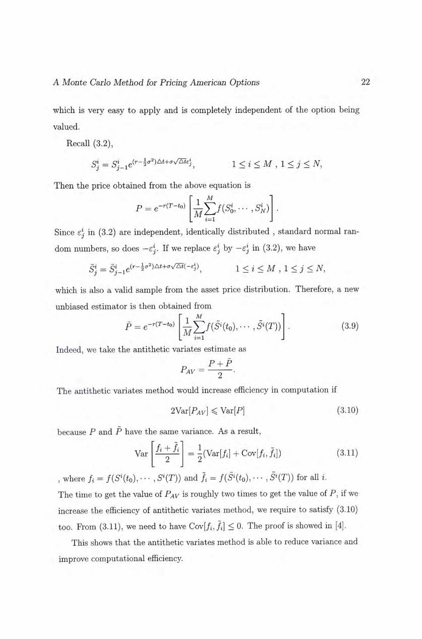
Recall (3.2),
Si = 1 < z < M , 1 < j < TV,
Then the price obtained from the above equation is
� 1 M 1
Since ej in (3.2) are independent, identically distributed , standard normal ran-
dom numbers, so does — ej. If we replace Sj by —Sj in (3.2), we have
= 苟 ( - 4 ) , l < z < M , l < j <iV,
which is also a valid sample from the asset price distribution. Therefore, a new
unbiased estimator is then obtained from � 1 M 1
P = e - 炉 知 ) ^ f . (3.9) . i=l -
Indeed, we take the antithetic variates estimate as
p x 「 宇 .
The antithetic variates method would increase efficiency in computation if
2Var[iV] < Var[P] (3.10)
because P and P have the same variance. As a result,
Var ^ ^ = i ( V a r [ / , ] + C o v [ / „ / , ] ) (3.11)
,where =麟to),…,分(T)) and = /(孕(力o),…,办(T)) for all i�
The time to get the value of Pav is roughly two times to get the value of P, if we
increase the efficiency of antithetic variates method, we require to satisfy (3.10)
too. From (3.11), we need to have Cov[/i, fi] < 0. The proof is showed in [4:.
This shows that the antithetic variates method is able to reduce variance and
improve computational efficiency.

Chapter 4
Cell Partition Method
In this chapter, we estimate the value of an American put option by partitioning
the payoff into tractable cells. We also use transition probability matrices to get
the value of an American put option by a backward algorithm. There is another
way for the partition the payoff into cells, see [1,2]. In [1], numbers of cells at
each time steps remains unchanged and the height of each cell increases at each
time step.
4.1 An Advantage of the Cell Partition Method
Its difficult to value an American put option because we need to estimate its
optimal exercise policy. Standard simulation procedures are forward algorithms.
A simulation generates the path paths forward in time. However, the pricing of
an American option uses a backward algorithm. The optimal exercise strategy at
the expiration date T is easily determined if it is in the money, that is K > S(T)
for a put option. Progressing backward in time, the optimal exercise strategy is
to compare the immediately exercise price and the discounted expected cash flow
from holding onto the option. That is
P{S{t),t) = max(i^ — S{t),E{P{S{t + At),t + At))), (41)
23

A Monte Carlo Method for Pricing American Options 24
where E{-) is the discounted expected value of the option at time t + At; and
P is a non dividend paying American put. One exercise it immediately if the
exercise value, max(K - S{t),0) > E{P{S{t + At),t + At)). In other Monte
Carlo methods for pricing an American option, they save all intermediate asset
prices for the computation in the early exercise strategy. Therefore, the storage
size is MN, where N is the number of time steps and M is the number of paths.
Moreover, the storage size depends on both N and M. If we have more time
steps or simulate more paths, then the storage size increases accordingly. We
cannot use too large M to prevent out of memory for the computer to run the
result by this method. In our method, the main idea of our method is using a
transition probability matrix to determine it. We first use grid to partition the
time and the paths into cells. Then we need to find the transition probability
Pt^t+At at two consecutive time steps t and t -h At, by counting the number of
paths passing through the cell at time t, say a and the number of paths moving
from the cell at time t to the cell at time t + At, say b, then the transition
probability pt,t+At = b/a. The transition probability matrix Pt,t+At is formed by
getting all transition probabilities pt,t+At for each cell between two consecutive
time steps t and t + At and the size of it is denoted by kf. So the main advantage
of our method is only to store the probability matrix instead of all the asset
prices. The storage size of our method is cN, where c is sum of the square of
kt^ c = J2t t- Therefore, the storage size of our method is independent on the
number of simulated paths.
4.2 The Algorithm
1. Generating the paths
In section (3.2), we have mentioned how to use the Monte Carlo method to
simulate the price paths. Using the equation (3.2),we need to generate a

A Monte Carlo Method for Pricing American Options 25
standard normal random number at each time step on each path. We use the
computer language, MATLAB, to do this. It has a built-in function "randn"
to generate these random numbers. Using antithetic variates method in
section (3.3), once we get a random number x to generate a path, we can
generate the other path by using, —x.
2. Partitioning the state space
Suppose we want to generate with M paths and M antithetic paths with
N time steps, the current asset price is /So, the current time is to and the
expiration date is T. We use the grid to partition the time and the paths into
numbers of cell. Each cell has the same, fixed height and width, we divide T — to
the partition in each time step tj, where tj =亡o + jAt, At 二 ~ — ~ and
the payoff is divided into Xj with the fixed height S, where Xj = Xm— + kS.
Xmirij denotes a minimum point at time tj. We also let Xmaxj to be a
maximum point at time tj. A procedure for the partition is as follow:
(a) To achieve the confidence interval 99.95%, we set a 二 3.27 in the
equation at each time step
Xmin] = S欣——ly��卜拳-犯�j—Y�^ , , � ,1 < j < AT. 4.2
I Xmax, = 5;3e(卜i内(H)射时()-l)^/^ ——
Since the value of an American put must greater than or equal to zero,
so Xmirij > 0.
(b) The finite partition at time tj is Cj where Cj = {Cj, C|, • ^ • , Cj^), 'Xmaxj — XminA . .丄 •上i 「一i j � i .r
Qj — ^― IS an integer with [x\ and [x\ are the ceiiing
of X and the floor of x respectively, [x] is the nearest integers that
larger than x and [x] is the nearest integer that smaller than x. Cj

A Monte Carlo Method for Pricing American Options 26
satisfies
‘ k [Xmaxj] — [Xmirij
< i d , = ^ (4.3) � C ^ n C ' j = 0 , for all k ^ L
That is the cell Cj with width from time j to time j +1 and the height
from a;)—1 to x^j hr 1 < k < 历,0<j<N.We can find k by
'(Si-XminX k= - , A 3 )\
where aS] is the value of an underlying asset at time tj at the z-th path.
For time to, the value of an underlying asset is the current asset price
S'o- There is only one partition Cq 二 {S'o}.
3. Transition Probability Matrices
We only need to use two consecutive time steps to get one transition prob-
ability matrix. For two consecutive time steps tj and tj+i, the transition
probability Pjj+i'-
/幻o,o 0,1 . . . \ PjJ+i Pj,j+i
p _ PjJ+l . . . • • •
\Pj,j+l 巧,J+1
where (hkl
P^i+i =\ 4 … (4.4) 0 , otherwise,
with a � i s the number of paths passing through Cj and 6芯十丄 is the number
of paths moving from CJ to Cj+i. Suppose there are M paths {^j ,…,Sf}fLi
A Monte Carlo Method for Pricing American Options 27
and M antithetic paths . . . , Sfjf^^, then aj and bfj^^ are:
4 = Card{z G [1,M]J G [1, N], S] G C;",S} G C^}
hki — V 1
Summation the transition probability over the I at each time tj, we see that
it must be equal to 1. That is
V^ k,i 1
l^P/j+i 二 1-I
4. Backward Algorithm
Now, we calculate an American put option from the expiration date T to
the current time to by a backward process.
(a) The value of American put option for the “ h path at the expiration
date T is
N) = max(i^ - S},, 0), for 0 < z < M, (45)
where Sj is the value of that in the cell Cj, we define Sj is the mean
value of cc广 1 and Xj for 1 < k < Qj and 0 < j < A .
� x ^ r ^ + x) 二� ^
3 2 =Xmiuj + (A: + 0.5)( .
(b) At time t^-i (i.e. t^ - At), comparing the immediately exercise price
max(K — 0) and the price from the expected cash flow from
视AO:
P(总—1, N-l) = max(ir — E 喊 N , 现 (4�6)
where N))) is the discounted expected value from N):
洲=E (力Li X P(苏,iV)e-(询). I
A Monte Carlo Method for Pricing American Options 28
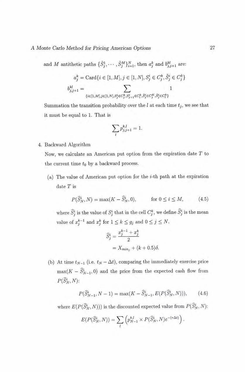
(c) Repeat step (b) recursively, backward in time,
‘ P { S i , j ) = max(i^ —蜀,E�P 尚+1�+ 1))),
^ E 喊 + 1)) = E X P(蜀+1, + ,
. I
f o r i e [0,iV — 1], i e [0,M],
to compute all the prices N -2), iV - 3), . . . , P{Sq, 0).
The price P(5o, 0) is our desired result at time to-
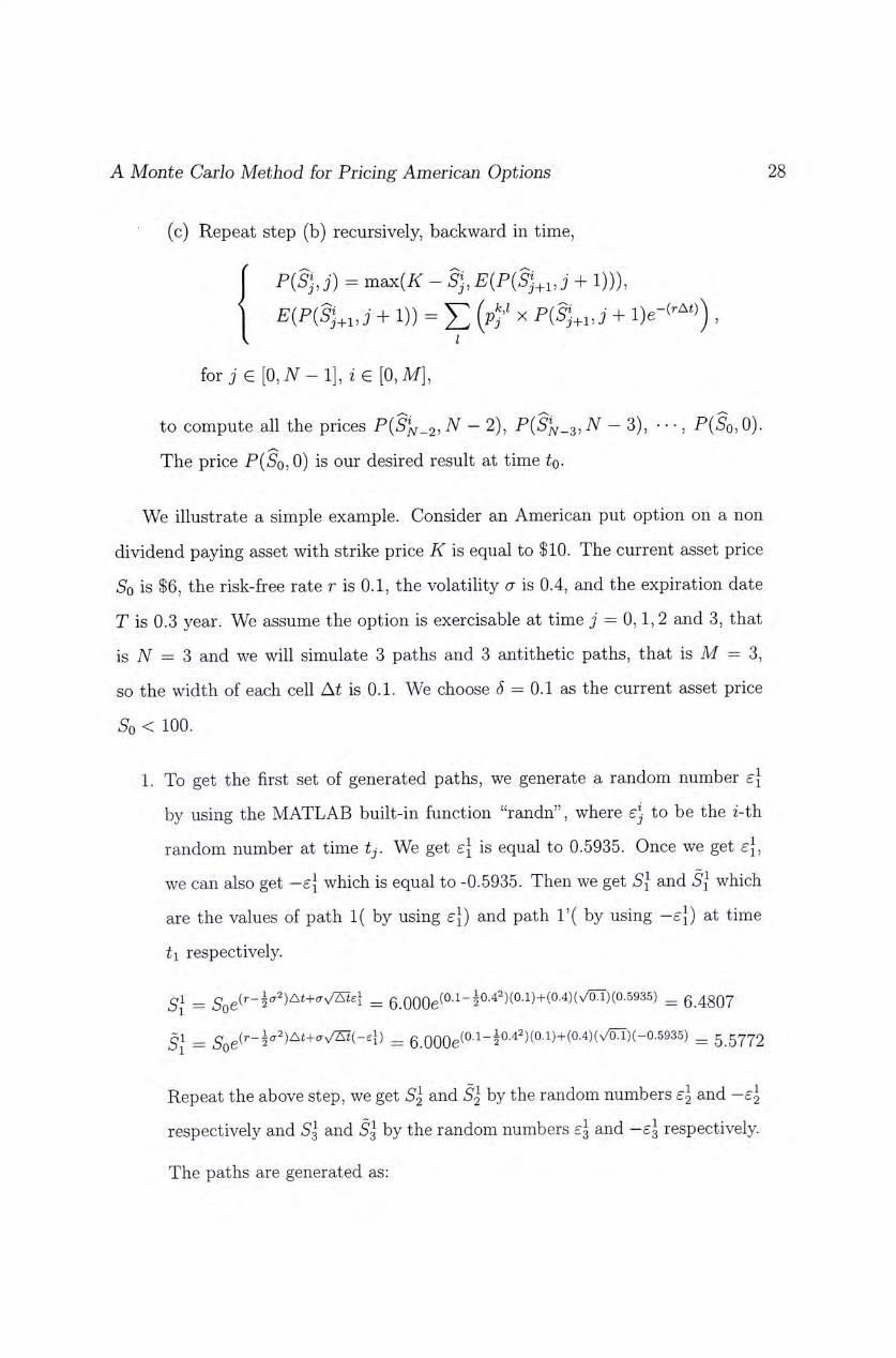
We illustrate a simple example. Consider an American put option on a non
dividend paying asset with strike price K is equal to $10. The current asset price
So is $6, the risk-free rate r is 0.1,the volatility a is 0.4,and the expiration date
T is 0.3 year. We assume the option is exercisable at time j = 0,1,2 and 3, that
is N = 3 and we will simulate 3 paths and 3 antithetic paths, that is M = 3,
so the width of each cell At is 0.1. We choose S = 0.1 as the current asset price
So < 100.
1. To get the first set of generated paths, we generate a random number ej
by using the MATLAB built-in function "randn", where £j to be the i-th
random number at time tj. We get e\ is equal to 0.5935. Once we get e},
we can also get -£\ which is equal to -0.5935. Then we get and S} which
are the values of path 1( by using el) and path l '( by using -e\) at time
ti respectively.
= = g_QQQg(0.1- i0 .42) (0 .1)+(0.4) (V^)(0 .5935) = 6.4807
二 二 g .oOOe^.l —全••42)(0-l) + (0.4)(V^)(_0.5935) = 5.5772
Repeat the above step, we get S2 and §2 by the random numbers s^ and - e l
respectively and S^ and §1 by the random numbers el and - e l respectively.
The paths are generated as:

A Monte Carlo Method for Pricing American Options 29
Path i SQ S^ S^ S^
1 6.0000 6.4807 6.7572 6.4813
1' 6.0000 5.5772 5.3705 5.6215
Similarly, we get path 2, path 2', path 3 and path 3'.
Path i Sq S^ S2 S^
2 6.0000 5.7262 5.3813 4.9347
2' 6.0000 6.3121 6.7436 7.3834
3 6.0000 5.5253 5.4128 5.8155
3' 6.0000 6.5254 6.7043 6.2651
2. By (4.2), we get Xmirij and Xmaxj:
j=Q j = l j 二2 j 二3
XmaXj 6.0000 9.0919 10.8126 12.3565
Xmirij 6.0000 3.9754 3.3562 2.9486
(a) In order to find the partition Cj where Cj = (Cj, • • • , C,), where XmaXj — XminA Qj — — ,we need to find g�first.
'fXmaxi-XminA] [/9.0919 - 3.9754\ 1 _
仍 = [ [ S )\ = K 0.1 Jj 二 双
‘ f Xmax2 - Xmin2\] |Y 10.8126 - 3.3562�1 „ 仍 = K ^ J J = K 0 . 1 ) \ = 7 5 ,
' f Xmax3 - Xmins\] |Y 12.3565 — 3.3562�1 _
仍 - ^ ) \ = ll""""O^jJ 二 95-For each Sp for all j , 2 < z < 3, we should find k from Cj. At time
to, we only have 1 cell in Cq. '(Si-XminX
Jc — �
LV ^ )\ The values of k are showed in Table 4.1.

A Monte Carlo Method for Pricing American Options 30
Path i k,S{ e Cf k, Si e k, SI e
1 26 35 36
1, 17 21 27
2 18 21 20
2' 24 34 45
3 16 21 29
3, 26 34 34
Table 4.1: the value of k, where G C^
3. Find the transition probability matrix
Once we get k, we are able to find the values of a � a n d 吟‘州 for j = 0,1, 2.
For j = 0,aj = 6 and
1 , if / = 16,17,18,24,
佑 = 2 , if / = 26, 0 , otherwise.
\
Therefore,
‘ I , if / = 16,17,18,24,
pli =臺,in = 26, 0 , otherwise.
\
For j = 1, f
1 , if A: = 16,17,18,24,
(A = < 2 , if /c = 26, 0 , otherwise.
V
and blf = bUf = = = blf = blf = 1,otherwise b�;^ = 0.
Therefore, ‘ 16,21 — 17,21 一 18,21 — 24,34 —
Pi,2 = Pi,2 二 Pi,2 — Pi,2 —丄,
< 26,34 _ 26,35 _ 1
]Pi,2 — Pi,2 — 2 ,
Pi'2 = 0 , otherwise.
A Monte Carlo Method for Pricing American Options 31
For J = 2, z
1 , if /c = 35,
, 2 , if A; = 34,
3 , if A: = 21,
0 , otherwise. V
and blf = hlf = blf 二 blf = b'^f = blf = 1, otherwise 6�:^ = 0.
Therefore,
‘2 1 , 2 0 — 21,27 — 21,29 — 1 ^2,3 — ^2,3 一 •^2,3 — 3 '
34,34 34,45 1
I 35,36 1 2,3 = 1,
P2 3 = 0 , otherwise. V ,
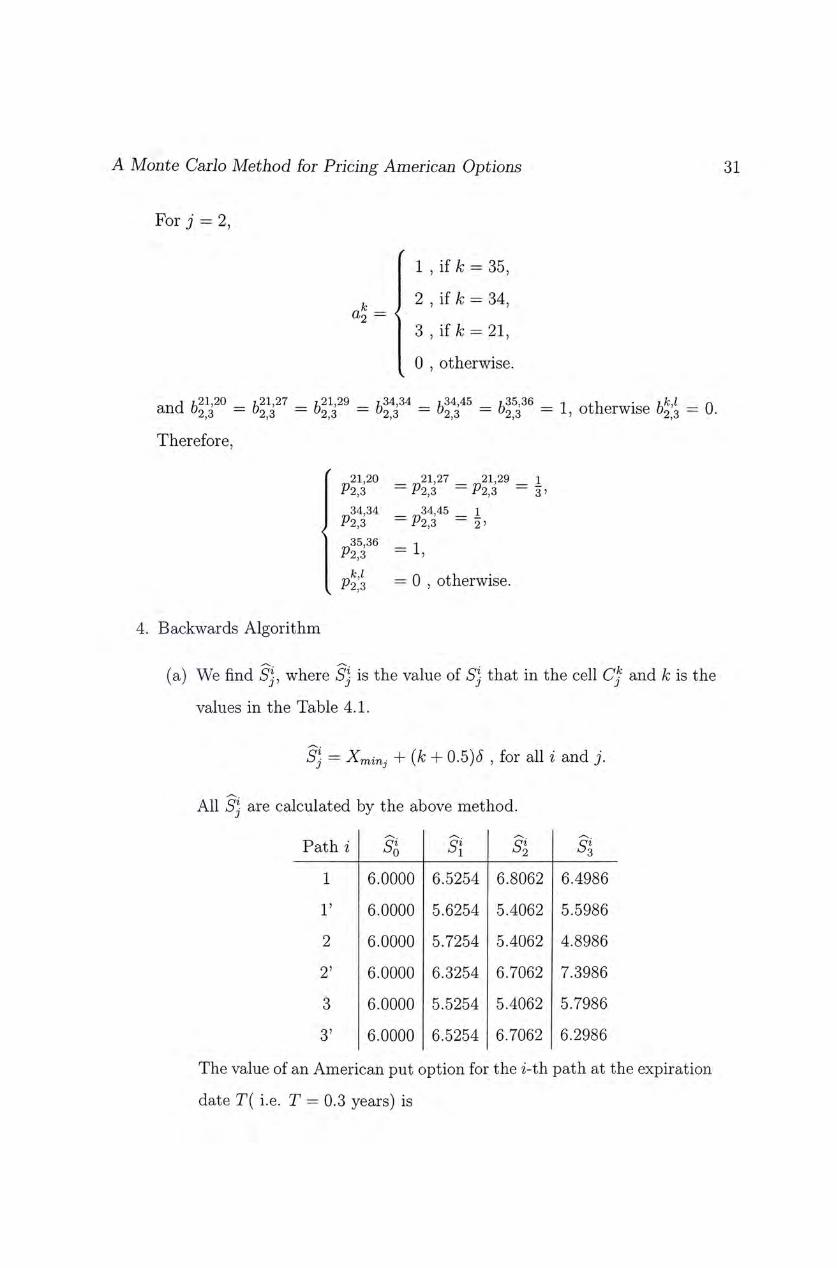
4. Backwards Algorithm
(a) We find 5], where Sj is the value of Sj that in the cell Cj and k is the
values in the Table 4.1.
Sj = Xmirij + (/c + 0�5)5 , for all i and j.
八.
All S�j are calculated by the above method.
Pclijll 2 /S'q S
1 6.0000 6.5254 6.8062 6.4986
1' 6.0000 5.6254 5.4062 5.5986
2 6.0000 5.7254 5.4062 4.8986
2' 6.0000 6.3254 6.7062 7.3986
3 6.0000 5.5254 5.4062 5.7986
3' 6.0000 6.5254 6.7062 6.2986
The value of an American put option for the i-th path at the expiration
date T( i.e. T = 0.3 years) is

A Monte Carlo Method for Pricing American Options 32
Path i Si P{Si 3) = max(ir —离,0)
1 6.4986 3.5014
1' 5.5986 4.4014
2 4.8986 5.1014
2' 7.3986 2.6014
3 5.7986 4.2014
3' 6.2986 3.7014
We have in step 4(a). For each path i, compute the value of the
payoff at each time step tj, that is comparing between the immediately
exercise price {K—Sj, 0) and the price from the expected cash flow from
holding onto the option,丑(P(蜀+” j+1) ) = ^ (p," x + 1)6—一)) I
to see if we should exercise.
(b) The following table is showed the result for time t2 (i.e. j = N — 1).
Holding Exercising
Path i E{P{Sl 3)) max(K — % 0)
二 !:(喊离,3K(圳) I
1 3.4666 3.1938
1' 4.5226 4.5938
2 4.5226 4.5938
2' 3.1200 3.2938
3 4.5226 4.5938
3' 3.1200 3.2938
For those paths we need exercise, we update P{Sl, 2) by the immedi-
ately exercise price, that is
万2 / max(X - SI 0) , if max(i^ — 0) > E{P(S l 3)) unchanged , otherwise
V

A Monte Carlo Method for Pricing American Options 33
Path i Exercise? Updated P(Sl 2)
1 No unchanged
1' Yes 4.5938
2 Yes 4.5938
2' Yes 3.2938
3 Yes 4.5938
3' Yes 3.2938
Repeat the above step to find P(Sl, 1),
Holding Exercising
Path i E{P{Sl 2)) max{K - Si 0)
I :
1 3.3466 3.4746
1' 4.5481 4.3746
2 4.5481 4.2746
2' 3.2610 3.6746
3 4.5481 4.4746
3' 3.3466 3.4746
For those paths we need exercise, we update 1) by the immedi-
ately exercise price, that is
3 / m^x{K-Sl,0) ,ifm^x{K-SlO)>E{P{Sl2))
I unchanged ,otherwise

A Monte Carlo Method for Pricing American Options 34
Path i Exercise? Updated F(Sl 1)
1 Yes 3.4746
r No unchanged
2 No unchanged
2' Yes 3.6746
3 No unchanged
3, Yes 3.4746
Finally we can find 0), the immediately exercise price at time to
is max{K — So, 0)=4 and the price from the expected cash flow from
holding onto the option,
E{P{Sl 1)) = X ] (pli X P{Sl I
=4.0044.
Therefore, the value of the American put option in this example is
$4.0044.
From the above example, we notice that the storage size of our method is
only Since Y^^Jo iOjOj+i) is fixed, the memory is 0{N) which
depends on N only. No matter how we change the number of paths, the storage
size remains unchanged. Therefore, we are able to have a large number of paths
without the problem for the machine being out of memory. We also notice that
the computation time is proportional to M x + 二i(邮j+i) x d. We have the
term M x d from generating M paths, the second term is due to the backward
algorithm in the early exercise strategy.

Chapter 5
Numerical Results
In this chapter, we provide some numerical results to illustrate our method. Our
results will compare with an example given in [8, p.335]. It is an American put
option with strike price K equals to $10,the risk-free rate r is 0.1, the volatility
a is 0.4 and the expiration date T is 0.5 years.
In our experiment, all the simulations were run with a processor, pentium III,
running at a clock rate of 1 GHz, and with 256 Megabyte of main memory. The
number of paths is M,, where M' = 2M( M paths plus M antithetic paths) and
the number of time steps is N. c equals to where (外办十丄)is the
size of the probability matrix Pj j i-
By using the antithetic variates method( AVM) in our method, table 5.1 shows
the effect on the errors by increasing M' paths from 1,000 to 100,000 and N is
fixed. In the table, the results computed by the Crank-Nicolson method are listed
in the column "CNM" and are taken from [8, p.335]. "Mean" and “STD” are the
means and the standard derivations obtained from 10 simulations. "Difference"
is the difference between the "CNM" and the "Mean". The table shows that
increasing M' paths 100 times, the standard derivations are smaller. Moreover,
the error decreases by one decimal point. This agrees with the rate of convergence / \
of the Monte Carlo method being O •
35

A Monte Carlo Method for Pricing American Options 36
M' = 103 M, = 105
So CNM Mean STD Difference Mean STD Difference
2 8.0000 8.0030 0.0007 0.0030 8.0028 0.0002 0.0028
4 6.0000 6.0010 0.0013 0.0010 6.0000 0.0000 0.0000
6 4.0000 4.0029 0.0016 0.0029 4.0000 0.0000 0.0000
8 2.0951 2.1416 0.0102 0.0465 2.1015 0.0009 0.0064
10 0.9211 0.9613 0.0022 0.0402 0.9283 0.0009 0.0072
12 0.3622 0.3905 0.0110 0.0283 0.3661 0.0013 0.0039
14 0.1320 0.1549 0.0087 0.0229 0.1336 0.0007 0.0016
16 0.0460 0.0556 0.0050 0.0096 0.0468 0.0006 0.0008
Table 5.1: CPM with N 二 100, M' = 10 and M' = 10 and using AVM
In table 5.2, "CPU" is the time in second to compute one result. It shows
the effect on the standard derivations obtained and the time after 10 simulation
by using antithetic variates method. From the table, we observe that there are
improvements in the error and the standard derivation for each SQ, and the time
for running one result is also faster by using the antithetic variaties method.
Without using the antithetic variates method, we need to generate 2M paths, so
the computational time is proportional to (2M + c)N. However, we only need to
generate M paths, then M antithetic paths is generated by using the antithetic
variates method, so the computational time is (M + c)N.
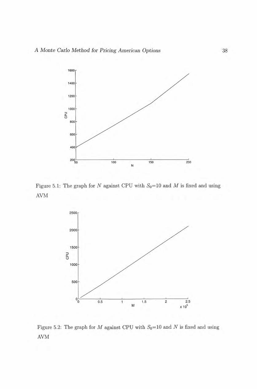
In table 5.3,we fix M' and change N. SQ equals to 10. We plot a graph N
against CPU in Fig. 5.1. We see that the graph C P U : (M + c)N is not linear
because c does not increase linearly.
Table 5.4 shows fixed N and M' is changed. SQ equals to 10. As N is fixed, c is
also fixed. We plot a graph M( but not M') against CPU in Fig. 5.2. We see that
the time increases linear as M increases linearly. This satisfies the computational
time is (M + c)N.

A Monte Carlo Method for Pricing American Options 37
without antithetic variates method with antithetic variates method
So CNM Mean STD Error CPU Mean STD Error CPU
2 8.0028 8.0028 0.0002 0.0028 590.6503 8.0028 0.0002 0.0028 535.3217
4 6.0000 6.0000 0.0000 0.0000 660.8883 6.0000 0.0000 0.0000 584.6208
6 4.0000 4.0000 0.0000 0.0000 737.1379 4.0000 0.0000 0.0000 632.6015
8 2.0951 2.1114 0.0021 0.0163 813.9074 2.1015 0.0009 0.0064 686.3169
10 0.9211 0.9306 0.0025 0.0095 910.9969 0.9283 0.0009 0.0072 736.9736
12 0.3622 0.3662 0.0019 0.0040 983.7516 0.3661 0.0013 0.0039 787.3481
14 0.1320 0.1340 0.0011 0.0020 1061.2600 0.1336 0.0007 0.0016 841.1895
16 0.0460 0.0470 0.0007 0.0010 1099.0000 0.0468 0.0006 0.0008 904.1803
Table 5.2: CPM with N = 100, M' = 10
2M 105
N 50 100 150 200
MEAN 0.9373 0.9283 0.9453 0.9492
CPU 395.9953 736.9736 1087.2900 1550.7800
Table 5.3: CPM with fixed M' and N is changed and using AVM
2M 104 5 X 10⁴ 105 5 X 10⁵
N 50
MEAN 0.9466 0.9391 0.9373 0.9364
CPU 37.7690 194.8232 395.9953 2108.5200
Table 5.4: CPM with fixed N and M' is changed and using AVM
A Monte Carlo Method for Pricing American Options 38
1600�
1400-
1200 - y / "
1000 - ^ ^
800 - ^ ^
6 0 0 -
400 Z
2 0 0 ' ‘ ‘ ‘
50 100 150 200 N
Figure 5.1: The graph for N against CPU with aSq二 10 and M is fixed and using
AVM
2500「
2000 -
1500-
1000 -
500 -
o' 1 1 ‘ ‘ ‘ 0 0.5 1 1.5 2 2.5
M X105
Figure 5.2: The graph for M against CPU with 二 10 and N is fixed and using
AVM

Chapter 6
Conclusion
The main difficulty in pricing American options is to estimate an optimal exercise
strategy. The optimal strategy is to compare the immediately exercise price and
the discounted expected cash flow from holding onto the option:
P(5(t), t) = max(i^ S{t), E{P{S{t + At),t + At)))
Generally, we need to save all intermediate asset prices for the computation in
the early exercise strategy using Monte Carlo method. It results in huge memory.
It depends on both the number of path M and the number of time steps N, In
this thesis, we get a better method in pricing American options. The method is
using probability matrices for pricing an American option. The advantage of our
method is that the storage size is only O(A^), so we can get a more accurate result
by increasing number of paths M without increasing the memory. Therefore, we
can have more numbers of paths to improve accuracy of the result without getting
the problem for the computer being out of memory.
Furthermore, the computation time increases linearly with the number of
paths. With the use of the variance reduction technique, we show that it reduces
the variance of our result. Numerical results illustrate the rate of convergence is
O ( for M' 二 2M, M paths plus M antithetic paths) and demonstrate the
39

A Monte Carlo Method for Pricing American Options 40
viability of our method. Our method is accurate and easy to apply on American
options. It can also be applied to higher dimensional option pricing problems.

Bibliography
.1] J. Barraquand and D. Martineau, Numerical Valuation of High Dimen-
sional Multivariate American Securities, Journal of Financial and Quani-
tative Analysis, 30 (1995), 383 — 405.
2] M. Broadie and P.Glasserman, A Stochastic Mesh Method for Pricing High-
Dimensional American Options, working paper, Columbia University.
3] M. Broadie and P.Glasserman, Pricing American-style securities using
simualUon, Journal of Economics and Control, 21(1997), 1323-1352
4] M. Broadie, P. Boyle and P. Glasserman, Monte Carlo Methods for security
pricing, Journal of Economics and Control, 21 (1997), 1267-1321
5] C. Cox, A. Ross and M. Rubinstein, Option Pricing: A Simplified Approach,
Journal of Financial Economics, 7(1979), 229-263
6] F. Giordano, M. Weir and W. Fox, A first course in Mathematical Modeling,
Brooks/Cole, 1985
7] P. Wilmott, Derivatives: the theory and pratice of financial engineering,
Wiley, 1998.
8] P. Wilmott, J. Dewynne and S. Howison, Option pricing : mathematical
models and computation , Oxford ,1993.
41


EbTiiOhOO
i ••llllllll saLjejqi-n >IHn3
m