Embed Size (px)
Citation preview
This is page 1Printer: Opaque this
Pressure matching forhydrocarbon reservoirs: a casestudy in the use of Bayes linearstrategies for large computerexperiments
Peter S. CraigMichael GoldsteinAllan H. SeheultJames A. Smith
ABSTRACT In the oil industry, fluid flow models for reservoirs are usuallytoo complex to be solved analytically and approximate numerical solutionsmust be obtained using a ‘reservoir simulator’, a complex computer pro-gram which takes as input descriptions of the reservoir geology. We describea Bayes linear strategy for history matching; that is, seeking simulator in-puts for which the outputs match closely to historical production. Thisapproach, which only requires specification of means, variances and covari-ances, formally combines reservoir engineers’ beliefs with data from fastapproximations to the simulator. We present an account of our experiencesin applying the strategy to match the pressure history of an active reservoir.The methodology is appropriate in a wide variety of applications involvinginverse problems in computer experiments.
1 Introduction
This paper describes and illustrates, by means of a case study, a Bayes linearapproach, incorporating expert knowledge, to matching historical hydro-carbon reservoir production using simulators of the reservoir. A reservoirsimulator is a complex computer program for solving the time-dependentpartial differential equations used to model oil, gas and water flow throughan operating reservoir. It takes as input various aspects of reservoir geologyand reservoir operation, including spatial distributions of rock propertiesand details of well locations and operating conditions. It returns as outputvarious measures of production, mostly in the form of time series; in par-ticular, oil, gas and water and pressures measured at the different wells.We are concerned with finding geology inputs for which simulator outputclosely matches observed historical production and, in particular, in this
2 Peter S. Craig, Michael Goldstein, Allan H. Seheult, James A. Smith
study, we aim to match the historical record of pressure readings from anactive reservoir.
Pressure matching is the first stage in a more general process of historymatching, in which we seek a reservoir geology which yields as close amatch as possible to the historical record for a wide variety of productionvariables. This search is carried out by running the simulator at differentinput settings until, hopefully, an acceptable match is found. The task iscomplex as the input and output spaces are very high dimensional, theremay be many or no acceptable matches, and the simulator is expensive inCPU time for each run. In the case study, we considered 40 input variablesand 77 output variables, and a simulation on our computer could take upto three days.
History matching is an example of a wide class of difficult practical prob-lems involving high dimensional searches in complex computer experiments.Such computer experiments have the special feature that repeated runs atthe same input settings always produce the same output, so that the clas-sical concept of random error is not present; an overview of the field isgiven in [SWMW89]. We shall describe a quite general approach to pres-sure matching, which may be similarly applied to many related types ofcomputer search problems. Our approach to prior specification is basedaround combining expert judgements of reservoir engineers with informa-tion gained from the analysis of experiments comprising a large numberof runs on relatively fast simple versions of the simulator. For example, areservoir engineer might judge that an output variable, such as the pressureat a particular well on a particular date, may depend primarily on just a fewof the input variables, such as the permeabilities of neighbouring regions ofthe well. The engineer may also make assessments of magnitudes of mea-surement errors in the recorded production output. The simulator may bespeeded up in various ways: in the case study, we coarsened the spatial gridemployed to solve the fluid flow equations. The output from many relativelyinexpensive runs of the faster simulator is used to build simple descriptionsrelating simulator output to simulator input. The two sources of informa-tion are combined into a specific structure describing prior means, variancesand covariances for relationships between the simulator inputs and outputs,and these relationships are analysed and updated using Bayes linear meth-ods given the outputs from relatively few runs of the ‘full’ simulator. Bayeslinear methods (for an introduction, see [FG93]) only require specificationof prior expectations, variances and covariances for the random quantitiesof interest, without the need for probability distributions, and they canbe linearly updated given outputs on the full simulator. In this way, priorspecification and subsequent analysis, including design computations forselecting inputs to the full simulator, are tractable, especially in contrastwith frequentist and traditional Bayesian formulations.
Our intention is to describe both a general methodology and a case studywhich applies the methodology. A preliminary description of our strategy

1. Pressure matching for hydrocarbon reservoirs 3
in [CGSS96] gave various elements of the methodology with application toa small demonstration problem. In this paper, we apply the methodology topressure matching for an actual reservoir. Among the differences that followfrom the substantially larger scale of this application are that we need toconsider (i) issues related to measurement errors in the recorded history;(ii) differences between the actual reservoir and the simulator; (iii) thedetailed task of constructing the prior specification; and (iv) efficient waysto carry out the various computational steps in our procedures, involvinghigh dimensional search and belief summarisation tasks.
The paper is set out as follows. In Section 2, we describe some of thebackground to the history matching problem. In Section 3, we give detailsof the particular reservoir that is the concern of this study. In Section 4,we discuss the objectives for the study. In Section 5, we outline the gen-eral Bayes linear strategy that we shall follow for matching pressures. InSection 6, we describe the prior formulation that we shall use for relatingparticular geology inputs to pressure outputs. In Section 7, we explain howwe carried out the prior specification to quantify the various elements ofthe prior description. In Section 8, we develop the notion of an implausi-bility measure which we use as a basis for restricting the subset of inputgeologies which may yield acceptable matching outputs. In Section 9, wedescribe the diagnostics that we employ to monitor the various elements ofour prior description. In Section 10, we explain how we choose which simu-lator runs to make in order to narrow our search for acceptable matches. Ineach section, we illustrate the general account with the relevant steps forour case study, and in Section 11 we describe further practical details of thecase study. Finally, in Section 12, we make various concluding commentsabout the study.
2 History Matching
In the oil industry, efficient management and prediction of hydrocarbonproduction depends crucially on having a good fluid flow model of the reser-voir under consideration. The model, which is a complex system of time-dependent, non-linear, partial differential equations describing the flow ofoil, gas and water through the reservoir, is too difficult to be solved an-alytically. Instead, an approximate numerical solution is obtained using a‘reservoir simulator’, a computer code which takes as input physical descrip-tions of the reservoir, such as geology, geometry, faults, well placements,porosities and permeabilities, and produces as outputs time series of oil,gas and water production and pressures at the wells in the reservoir. Thecorresponding historical time series are mostly unequally spaced and thetimes at which the different series are recorded often do not correspond.The eventual aim is to find a setting of the input geology which results in

4 Peter S. Craig, Michael Goldstein, Allan H. Seheult, James A. Smith
a simulator run with outputs which match as closely as possible the corre-sponding reservoir history. This process is termed history matching and isdescribed in [MD90]. In the case study, we try to match recorded pressuresby varying permeabilities in the geologically distinct subregions that makeup the reservoir and by varying transmissibilities of faults which geologistsbelieve may exist at certain locations.
There are several reasons for carrying out a history match. First, we mayhope to predict future reservoir performance, using the given simulator.Secondly, we may intend to use the simulator as an aid to decision making,for example to help decide where to sink further wells. Thirdly, we may wantto make inferences about the physical composition of the reservoir whichmay be used in a more general context, for example as inputs into a moredetailed simulation study of the reservoir. Of most immediate relevance forthe approach that we shall develop are the following two distinctions:
1. Is the aim to find a single good history match, as is often the currentpractice, or is it to seek to identify the class of all possible historymatches, subject to some general criterion of match quality?
2. Is the aim to find history matches which are predictive for futurereservoir performance, or is it to find matches which are informativefor the composition of the reservoir?
We will discuss the consequences of these methodological distinctions inour development of the case study.
In practice, this inverse problem, namely choosing an appropriate inputgeology and perhaps making structural changes to the model so that thesimulator output matches historical time series, is tackled by reservoir en-gineers on a trial and error basis using all of their technical knowledge,experience and specific understandings of the particular reservoir understudy. At each stage, values are chosen for input geology settings, the sim-ulator is run, the production output is scrutinised and compared with his-torical production, and new settings for the geology inputs are suggested.This process is time consuming for two reasons. First, simulator run-timeis typically many CPU hours (between 1 and 3 days in our case study), sothat it is impractical to make large numbers of runs. Secondly, the outputfrom each run requires careful scrutiny in order to select the next choiceof input values at which to run the simulator. In many cases, a fully satis-factory match is not obtained and usually it is hard to judge whether thiswas due to a problem with the underlying model or due to an inadequatesearch over the space of possible inputs. It is hoped that, by formalisingaspects of the problem, (i) more efficient choices may be made for runs onthe simulator; (ii) the efforts of the reservoir engineer may be better spenton those aspects of the study which genuinely require expert intervention;and (iii) a rather more informative analysis can be carried out, involvingconsideration of the class of possible matches and associated uncertainties.

1. Pressure matching for hydrocarbon reservoirs 5
While we discuss these issues in the context of history matching, they aresimilarly relevant for the analysis of any large computer model.
3 Case Study
This case study concerns a large, primarily gas-producing reservoir, onewith which our industrial collaborators Scientific Software-Intercomp (SSI)have twice been involved. For reasons of commercial confidentiality, theidentity and location of the reservoir and certain other details cannot bedisclosed.
The reservoir covers an area of about 30km by 20km and is about 60metres thick. The main productive reservoir units are two sandy layers, atop layer of clean marine sand, and a more shaley bottom layer.
The reservoir comprises four fields. One field is mainly onshore with asmall part under shallow coastal waters, and the other three are offshorein progressively deeper water. Gas production has to date been solely fromthe onshore field, due mainly to the relative costs and ease of drilling.Historical performance suggests that the reservoir fields effectively behaveas one unit, pressure communication between individual fields being viathe hydrocarbon zones and/or common aquifers.
A reservoir description developed by SSI in 1993/94, covering the pro-duction period March 1972 to June 1993, formed the basis of the three-dimensional simulation model used in this case study.
3.1 Simulation Model Description
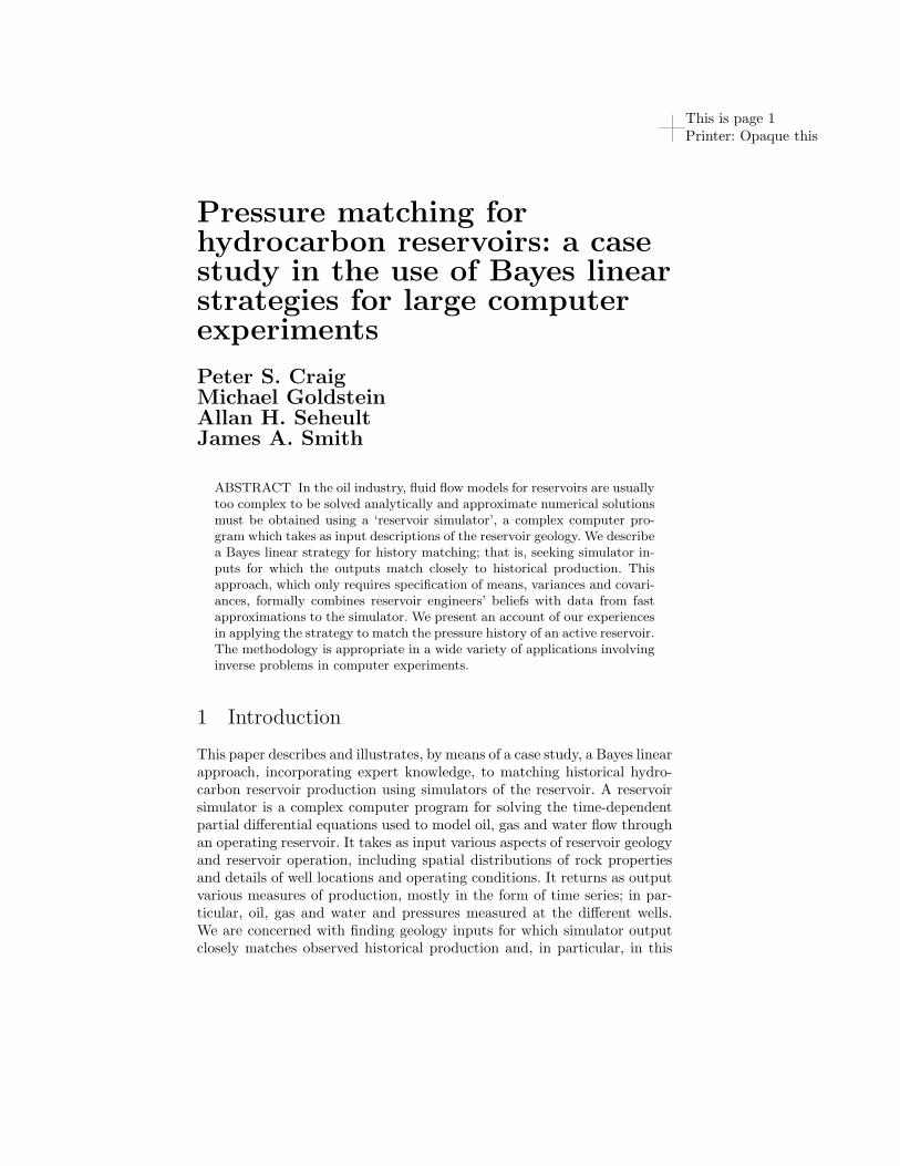
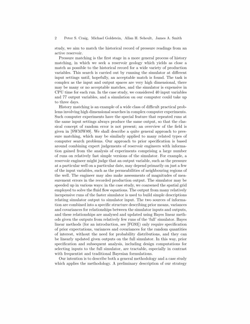
The reservoir description, which includes reservoir structure and geome-try, spatial distribution of porosity and fault patterns, was provided bySSI. Figures 1 and 2 show the extent of the two reservoir layers, and theapproximate location of wells and possible faults.
The initial spatial distribution of absolute permeability for this reservoirwas derived from the corresponding spatial distribution of porosity suppliedby the client oil companies. In the case study, the reservoir was divided intoseven sub-regions. For each sub-region a single multiplicative factor, varyingbetween 10−1 and 101, was used to modify the initial map. Permeabilitiesin the directions of the chosen horizontal orthogonal axes were taken tobe the same, while vertical permeability was taken to be 1% of horizontalpermeability. Porosity and other ‘parameter’ values supplied by SSI, suchas capillary pressures, were kept fixed throughout the case study.
Early simulation studies by SSI utilised a two layer model correspond-ing to the two sandy units. A five layer refinement with these two layersvertically subdivided was used by SSI in the later stages of their study. Inour study of the same field over the same production period, we used this
6 Peter S. Craig, Michael Goldstein, Allan H. Seheult, James A. Smith
1
2
3
4
5
6 7
8
9
1011
12
131415
16 17
18
1920
21
22
23
2425
26
2728
29
30
31 32
3334
35
36
37
38
3940
41
42
43
44
45
46
4748
49
50
8
10
12
13
14
15
16
17
18
19
21
23
2527 2727
29
313335
37
39
1(x1)
2(x2)3(x3)
4(x4)
5(x6)
Top layer of reservoir
1
2
3
4
5
6 7
8
9
1011
12
131415
16 17
18
1920
21
22
23
2425
26
2728
29
30
31 32
3334
35
36
37
38
3940
41
42
43
44
45
46
4748
49
50
9
11
12
13
14
15
16
17
18
20
22
24
2628 2828
30
323436
38
40
1(x1)
2(x2)
3(x3)
4(x5)
5(x7)
Bottom layer of reservoir
FIGURE 1. Maps of the layers of the reservoir (magnified maps of the western endof the reservoir are shown in Figure 2). Regions are indicated by regular hatchingand labelled by bold-face numbers. The corresponding simulator input variable,acting as permeability multiplier for the region, is shown in parentheses after theregion number . White space areas are not part of the reservoir. Possible faultsare indicated by thicker lines. A number on its side beside a fault indicates thevariable controlling the fault’s transmissibility. Wells with measurements used inthe study are located at the centre of the corresponding well number. Other wellsare indicated by dots.
1. Pressure matching for hydrocarbon reservoirs 7
1
2
3
4
5
6
7
8
9
10
11
12
1314
15
1617
18
19
20
21
22
23
24
25
26
27
28
29
30
3132
33
34
35
36
37
38
39
40
41
42
43
44
45
46
47
48
49
50
8
10
12
13
14
15
16
17
18
19
21
23
2527 27
27
29
3133
35
37
39
3(x3)
4(x4)
5(x6)
Top layer of reservoir
1
2
3
4
5
6
7
8
9
10
11
12
1314
15
1617
18
19
20
21
22
23
24
25
26
27
28
29
30
3132
33
34
35
36
37
38
39
40
41
42
43
44
45
46
47
48
49
50
9
11
12
13
14
15
16
17
18
20
22
24
2628 28
28
30
3234
36
38
40
4(x5)
5(x7)
Bottom layer of reservoir
FIGURE 2. Magnified maps of the western end of the reservoir. For details ofthe meaning of symbols, see Figure 1.
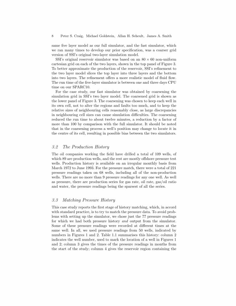
8 Peter S. Craig, Michael Goldstein, Allan H. Seheult, James A. Smith
same five layer model as our full simulator, and the fast simulator, whichwe ran many times to develop our prior specification, was a coarser gridversion of SSI’s original two-layer simulation model.
SSI’s original reservoir simulator was based on an 80 × 60 non-uniformcartesian grid on each of the two layers, shown in the top panel of Figure 3.To better approximate the production of the reservoir, SSI’s refinement tothe two layer model slices the top layer into three layers and the bottominto two layers. The refinement offers a more realistic model of fluid flow.The run time of the five-layer simulator is between one and three days CPUtime on our SPARC10.
For the case study, our fast simulator was obtained by coarsening thesimulation grid in SSI’s two layer model. The coarsened grid is shown asthe lower panel of Figure 3. The coarsening was chosen to keep each well inits own cell, not to alter the regions and faults too much, and to keep therelative sizes of neighbouring cells reasonably close, as large discrepanciesin neighbouring cell sizes can cause simulation difficulties. The coarseningreduced the run time to about twelve minutes, a reduction by a factor ofmore than 100 by comparison with the full simulator. It should be notedthat in the coarsening process a well’s position may change to locate it inthe centre of its cell, resulting in possible bias between the two simulators.
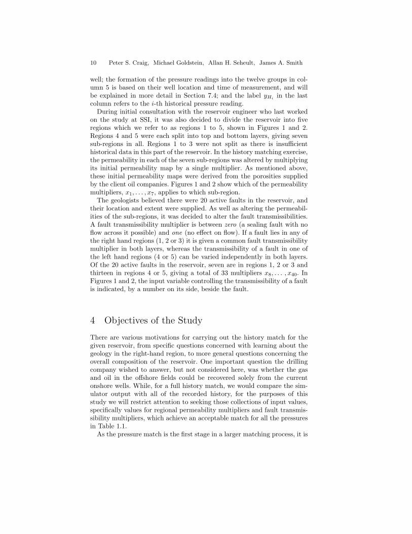
3.2 The Production History
The oil companies working the field have drilled a total of 109 wells, ofwhich 89 are production wells, and the rest are mostly offshore pressure testwells. Production history is available on an irregular monthly basis fromMarch 1972 to June 1993. For the pressure match, there were a total of 221pressure readings taken on 68 wells, including all of the non-productionwells. There are no more than 9 pressure readings for any one well. As wellas pressure, there are production series for gas rate, oil rate, gas/oil ratioand water, the pressure readings being the sparsest of all the series.
3.3 Matching Pressure History
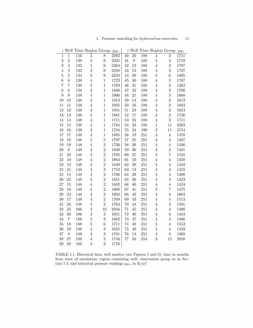
This case study reports the first stage of history matching, which, in accordwith standard practice, is to try to match the pressure data. To avoid prob-lems with setting up the simulator, we chose just the 77 pressure readingsfor which we had both pressure history and output from the simulator.Some of these pressure readings were recorded at different times at thesame well. In all, we used pressure readings from 50 wells, indicated bynumbers in Figures 1 and 2. Table 1.1 summarises this history: column 2indicates the well number, used to mark the location of a well in Figures 1and 2; column 3 gives the times of the pressure readings in months fromthe start of the study; column 4 gives the reservoir region containing the

1. Pressure matching for hydrocarbon reservoirs 9
Original Flow Simulation Grid
Coarsened Grid
FIGURE 3. Grids used for full and fast simulators of reservoir.
10 Peter S. Craig, Michael Goldstein, Allan H. Seheult, James A. Smith
well; the formation of the pressure readings into the twelve groups in col-umn 5 is based on their well location and time of measurement, and willbe explained in more detail in Section 7.4; and the label yHi in the lastcolumn refers to the i-th historical pressure reading.
During initial consultation with the reservoir engineer who last workedon the study at SSI, it was also decided to divide the reservoir into fiveregions which we refer to as regions 1 to 5, shown in Figures 1 and 2.Regions 4 and 5 were each split into top and bottom layers, giving sevensub-regions in all. Regions 1 to 3 were not split as there is insufficienthistorical data in this part of the reservoir. In the history matching exercise,the permeability in each of the seven sub-regions was altered by multiplyingits initial permeability map by a single multiplier. As mentioned above,these initial permeability maps were derived from the porosities suppliedby the client oil companies. Figures 1 and 2 show which of the permeabilitymultipliers, x1, . . . , x7, applies to which sub-region.
The geologists believed there were 20 active faults in the reservoir, andtheir location and extent were supplied. As well as altering the permeabil-ities of the sub-regions, it was decided to alter the fault transmissibilities.A fault transmissibility multiplier is between zero (a sealing fault with noflow across it possible) and one (no effect on flow). If a fault lies in any ofthe right hand regions (1, 2 or 3) it is given a common fault transmissibilitymultiplier in both layers, whereas the transmissibility of a fault in one ofthe left hand regions (4 or 5) can be varied independently in both layers.Of the 20 active faults in the reservoir, seven are in regions 1, 2 or 3 andthirteen in regions 4 or 5, giving a total of 33 multipliers x8, . . . , x40. InFigures 1 and 2, the input variable controlling the transmissibility of a faultis indicated, by a number on its side, beside the fault.
4 Objectives of the Study
There are various motivations for carrying out the history match for thegiven reservoir, from specific questions concerned with learning about thegeology in the right-hand region, to more general questions concerning theoverall composition of the reservoir. One important question the drillingcompany wished to answer, but not considered here, was whether the gasand oil in the offshore fields could be recovered solely from the currentonshore wells. While, for a full history match, we would compare the sim-ulator output with all of the recorded history, for the purposes of thisstudy we will restrict attention to seeking those collections of input values,specifically values for regional permeability multipliers and fault transmis-sibility multipliers, which achieve an acceptable match for all the pressuresin Table 1.1.
As the pressure match is the first stage in a larger matching process, it is
1. Pressure matching for hydrocarbon reservoirs 11
i Well Time Region Group yHi i Well Time Region Group yHi1 1 116 3 8 2292 40 20 188 4 3 17112 2 130 3 9 2335 41 9 188 4 3 17193 3 132 1 9 2364 42 12 188 4 3 17074 4 132 3 9 2350 43 13 188 4 3 17275 5 134 3 9 2234 44 29 188 5 6 16956 6 138 4 1 1723 45 30 188 4 3 17077 7 138 4 1 1769 46 31 188 4 3 13628 8 138 4 1 1880 47 32 188 4 3 17009 9 138 4 1 1906 48 21 188 4 3 1668
10 10 138 4 1 1913 49 14 188 4 3 161311 11 138 4 1 1925 50 16 188 4 3 168212 12 138 4 1 1941 51 23 188 4 3 162413 13 138 4 1 1881 52 17 188 4 3 172614 14 138 4 1 1711 53 24 188 4 3 171115 15 138 4 1 1784 54 33 188 1 11 226316 16 138 4 1 1784 55 34 190 2 11 215417 17 138 4 1 1885 56 19 251 4 4 137618 18 148 5 5 1797 57 35 251 4 4 140719 19 148 4 2 1736 58 26 251 4 4 143620 8 148 4 2 1839 59 36 251 4 4 150121 20 148 4 2 1785 60 37 251 5 7 154522 10 148 4 2 1864 61 10 251 4 4 145823 13 148 4 2 1849 62 38 251 4 4 144324 21 148 4 2 1752 63 13 251 4 4 145525 14 148 4 2 1706 64 39 251 4 4 139826 22 148 4 2 1851 65 30 251 4 4 142327 15 148 4 2 1682 66 40 251 4 4 142428 16 148 4 2 1668 67 41 251 5 7 147529 23 148 4 2 1682 68 42 251 4 4 166430 17 148 4 2 1769 69 43 251 4 4 151331 24 148 4 2 1784 70 44 251 4 4 150132 25 166 3 10 2016 71 45 251 4 4 149833 26 186 4 3 1651 72 46 251 4 4 143434 7 188 4 3 1662 73 47 251 4 4 146635 18 188 5 6 1711 74 48 251 5 4 155336 19 188 4 3 1635 75 49 251 4 4 143337 8 188 4 3 1701 76 14 251 4 4 136938 27 188 4 3 1716 77 50 254 3 12 201639 28 188 4 3 1716
TABLE 1.1. Historical data: well number (see Figures 1 and 2); time in monthsfrom start of simulation; region containing well; observation group as in Sec-tion 7.4; and historical pressure readings yHi, in lb/in2.

12 Peter S. Craig, Michael Goldstein, Allan H. Seheult, James A. Smith
important to identify the collection of possible geologies which may produceadequate pressure matches. In particular, it is useful to identify which ofthe input geology variables considered have little effect in determining thepressure match, as these may be varied in subsequent matching withoutaffecting the match on pressure. More generally, the collection of potentialmatches may be used to capture uncertainty about predictions for futurereservoir behaviour by running the simulator at different reservoir geologieswhich achieve acceptable match quality.
There are three views that we may take in assessing match quality. First,we may simply consider the difference between the observed history and theproduction output of the simulator. Secondly, as the observed history con-sists of true production values observed with error, we may seek to matchthe unobserved true production. Thirdly, we may consider that our goal isto identify the physical composition of the reservoir, in which case we mustalso incorporate into our comparisons the possible differences between thereservoir and the simulator. Although the first of these alternatives is usualpractice, it seems more natural to prefer the second, incorporating explicitassessment of errors in measurement. The choice between the second andthird view is less clear, however. If our intention is to predict future perfor-mance using the given simulator, then arguably it may be most efficient tochoose the best predictor of true production from the simulator. However,if the results of the match are to be used for other inferential purposes,and in particular if the estimated geology that is obtained by the match isto be used outside the context of the given simulation, then arguably weshould incorporate assessments of the differences between the reservoir andthe simulator into our matching procedures.
In this study, we shall mainly concentrate on matching true production,largely ignoring the differences between reservoir and simulator and assess-ing the quality of the match in terms of judgements, about measurementerrors in the pressure readings, that were provided by the reservoir engi-neer. Essentially, ignoring the differences between reservoir and simulator,avoids introducing an extra, and rather subtle, layer of modelling whichwould make it difficult, within the restrictions of the current account, toassess the success of our matching procedure. However, we could incorpo-rate such differences into our procedures in a similar way to measurementerror, and we shall indicate where such differences enter the analysis.
5 Bayes Linear Strategies for History Matching
In [CGSS96], some general strategies were outlined for tackling computerexperiments such as history matching. In this paper we further developthese strategies and describe their application to a particular reservoirstudy.
1. Pressure matching for hydrocarbon reservoirs 13
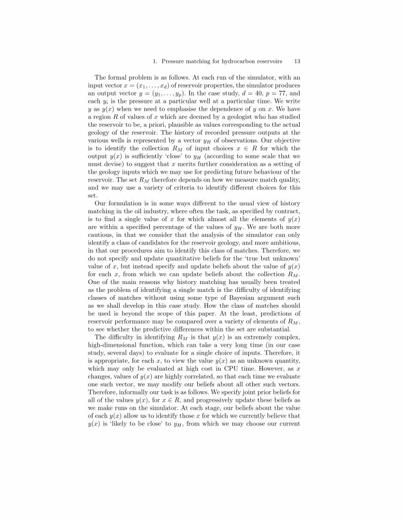
The formal problem is as follows. At each run of the simulator, with aninput vector x = (x1, . . . , xd) of reservoir properties, the simulator producesan output vector y = (y1, . . . , yp). In the case study, d = 40, p = 77, andeach yi is the pressure at a particular well at a particular time. We writey as y(x) when we need to emphasise the dependence of y on x. We havea region R of values of x which are deemed by a geologist who has studiedthe reservoir to be, a priori, plausible as values corresponding to the actualgeology of the reservoir. The history of recorded pressure outputs at thevarious wells is represented by a vector yH of observations. Our objectiveis to identify the collection RM of input choices x ∈ R for which theoutput y(x) is sufficiently ‘close’ to yH (according to some scale that wemust devise) to suggest that x merits further consideration as a setting ofthe geology inputs which we may use for predicting future behaviour of thereservoir. The set RM therefore depends on how we measure match quality,and we may use a variety of criteria to identify different choices for thisset.
Our formulation is in some ways different to the usual view of historymatching in the oil industry, where often the task, as specified by contract,is to find a single value of x for which almost all the elements of y(x)are within a specified percentage of the values of yH . We are both morecautious, in that we consider that the analysis of the simulator can onlyidentify a class of candidates for the reservoir geology, and more ambitious,in that our procedures aim to identify this class of matches. Therefore, wedo not specify and update quantitative beliefs for the ‘true but unknown’value of x, but instead specify and update beliefs about the value of y(x)for each x, from which we can update beliefs about the collection RM .One of the main reasons why history matching has usually been treatedas the problem of identifying a single match is the difficulty of identifyingclasses of matches without using some type of Bayesian argument suchas we shall develop in this case study. How the class of matches shouldbe used is beyond the scope of this paper. At the least, predictions ofreservoir performance may be compared over a variety of elements of RM ,to see whether the predictive differences within the set are substantial.
The difficulty in identifying RM is that y(x) is an extremely complex,high-dimensional function, which can take a very long time (in our casestudy, several days) to evaluate for a single choice of inputs. Therefore, itis appropriate, for each x, to view the value y(x) as an unknown quantity,which may only be evaluated at high cost in CPU time. However, as xchanges, values of y(x) are highly correlated, so that each time we evaluateone such vector, we may modify our beliefs about all other such vectors.Therefore, informally our task is as follows. We specify joint prior beliefs forall of the values y(x), for x ∈ R, and progressively update these beliefs aswe make runs on the simulator. At each stage, our beliefs about the valueof each y(x) allow us to identify those x for which we currently believe thaty(x) is ‘likely to be close’ to yH , from which we may choose our current

14 Peter S. Craig, Michael Goldstein, Allan H. Seheult, James A. Smith
candidates for the collection RM .We have at least three types of problem. First, we have a modelling
problem, in that we must find a way to develop joint prior beliefs aboutthe values of all of the outputs for all choices of inputs. As we can onlymake a relatively small number of evaluations of the simulator, these priorbeliefs must be sufficiently detailed and reliable to allow us to extrapolateour beliefs over the values of y(x) for x varying over the whole of the regionR, while still being of a sufficiently simple form both to allow for meaningfulelicitation and also to result in a tractable analysis. Secondly, we have adesign problem, in that we must at each stage be able to identify at whichvalues of the inputs to run the simulator, so as to maximise the amount ofinformation that we will gain about RM . Thirdly, in addition to the generalproblem of updating such a large collection of beliefs, we have a substantialpractical problem of inversion, which arises due to the high dimensionalnature of the simulator. Even if the function y(x) could be computed verycheaply for all x, there would still be a substantial numerical inversionproblem in identifying the region RM , and this difficulty is compoundedby the substantial uncertainty as to the value of y(x) for all values of x atwhich the simulator has not been evaluated.
Each of these problems is very difficult to tackle within a full Bayes for-malism: prior specification is difficult due to the extreme level of detailrequired for the joint prior distribution; full Bayes design calculations arenotoriously computer intensive, even for much more straightforward prob-lems; and probabilistic analysis and inversion is technically difficult for highdimensional joint distributions.
For these reasons, we choose an approach which is based around theideas of Bayes linear modelling and adjustment of beliefs. An overview ofBayes linear methodology, with applications, is given in [FG93]. The Bayeslinear approach is similar in spirit to the Bayes approach but, rather thanworking with full prior beliefs, we restrict attention to the specification ofprior means, variances and covariances between all quantities of interest.We update our beliefs by linear fitting on the data. In comparison withthe full Bayes analysis, in the Bayes linear approach it is therefore easierto make the required prior specifications and also more straightforward toupdate beliefs, both of which are crucial simplifications when analysingvery high dimensional sequential search problems.
The simplest form of the Bayes linear approach is as follows. We have twovectorsB andD. We specify directly, as primitive quantities, the prior meanvectors, E[B], E[D], and prior variance and covariance matrices, Var[B],Var[D] and Cov[B,D]. The adjusted expectation ED[B] and the adjustedvariance VarD[B] for B, having observed D, are given by
ED[B] = E[B] + Cov[B,D]Var[D]−1(D − E[D]) (1.1)VarD[B] = Var[B]− Cov[B,D]Var[D]−1Cov[D,B] (1.2)

1. Pressure matching for hydrocarbon reservoirs 15
If Var[D] is not invertible, then we use the Moore-Penrose generalised in-verse in the above equations. Adjusted expectations may be viewed as sim-ple approximations to full Bayes conditional expectations, which are exactin certain important special cases such as joint normality. An alternativeinterpretation of Bayes linear analyses, as those inferences for posteriorjudgements which may be justified under partial prior specifications, isgiven in [Gol96]. While there are important foundational reasons for us-ing the Bayes linear approach, our choice in this case study is made onpragmatic grounds. The full Bayes approach is too difficult to implementand our hope is that the Bayes linear approach will capture enough of theuncertainty in the problem to allow us to develop tractable and effectivestrategies for history matching.
Our general strategy, which is applicable to a wide variety of inverse prob-lems for large scale computer models, may be summarised in the followingsteps, which provide an overview of the methodology that we describe andapply in this study.
1. We elicit aspects of qualitative and quantitative prior beliefs by dis-cussion with a reservoir engineer. We only quantify prior means, vari-ances and covariances. We need to elicit two types of beliefs. First,we must consider the relationship between the observed history yHand the output from the simulator. Secondly, we must consider therelationship between input and output for the simulator. In principle,the elicitation should proceed as follows, though in practice we mayneed to approximate some of the steps.
(a) We must consider how closely we should expect to be able tomatch the observed history yH . There are two reasons why wemay not achieve a close match. First, the observations yH maybe considered to consist of a vector of true pressure values, yT ,observed with measurement errors, whose prior variances mustbe quantified. Secondly, there may be systematic differences be-tween the simulator and the reservoir, and means, variances andcovariances for such differences should be assessed. In this study,more attention was paid to representing measurement errorsthan to representing differences between the reservoir and simu-lator, but we shall discuss both types of representation and theissues involved in relating each of these assessments to matchquality.
(b) For each x, x′ ∈ R, we must elicit a prior mean vector and vari-ance matrix for y(x) and a covariance matrix between y(x) andy(x′). These mean and variance specifications are functions ofthe input vector. Given the high dimensionality of the problem,and the need for detailed investigation of the mean and variancesurfaces, we construct this prior specification by first eliciting
16 Peter S. Craig, Michael Goldstein, Allan H. Seheult, James A. Smith
simple qualitative descriptions which focus on the most impor-tant relationships between the inputs and the outputs. We there-fore seek to identify, for each component yi(x) of y(x), a smallsubset of components of x, termed the active collection of inputsfor yi, with the property that our beliefs about changes in thevalue of yi(x) resulting from changes in x are almost entirely ex-plained by the changes in the values of the active variables for yi.In the study, we found that, for each output quantity, the reser-voir engineer was willing to restrict attention to a collection ofthree active variables, which resulted in enormous simplificationsin the subsequent analyses. For each output, we must thereforeidentify the active inputs qualitatively, and then quantify priorbeliefs about the magnitudes of the effects of each active input,which we do by considering the following type of assessment:‘if the value of a particular input, xj say, changes by one unit,while holding all other inputs fixed at some central values, assessmeans and variances for the change in each component of y(x)for which xj is an active variable.’
(c) There is a third potentially useful source of prior beliefs thatmay be relevant to this problem, namely a prior specificationof beliefs about the physical geology. However, we did not haveaccess to the geologist who had been familiar with this reservoir,and the reservoir engineer was unwilling to express such beliefs.It was also his opinion that the geologist was unlikely to havestrong prior opinions.
2. Identifying active variables for each output and quantifying their ef-fects is a large, challenging and unfamiliar elicitation task. Therefore,we find it helpful to construct fast approximations to the original sim-ulator, which can provide additional information to guide our priorquantification. We make many runs on the fast simulators, for in-puts chosen within region R. In the case study, we could performroughly 200 runs on the fast simulator for the time taken by one runof the full simulator. By fitting linear models to the data from theruns on the fast simulator, we may quickly form a fairly detailed,albeit provisional, qualitative and quantitative picture of the rela-tionships between the input and the output variables. Our aim, asin the prior elicitation, is to construct simple descriptions, where weselect a small number of geology input variables which are most im-portant in explaining the variation for each pressure output variable,and then to build a prior description which expresses these relation-ships. The prior specification process that was followed for the casestudy resulted in choosing, for each output quantity, a maximum ofthree active input quantities and fitting a quadratic surface in thethree variables plus a spatially correlated residual structure.

1. Pressure matching for hydrocarbon reservoirs 17
3. We compare the choice of active variables from the prior elicitationand from the data analysis on the fast simulator, and combine theinformation from the two sources using a variety of informal judge-ments and formal methods based on quantities such as elicited beliefsconcerning the differences between the two simulators.
The overall result of our elicitation is (a) a specification of the re-lationship between the observed history and the output of the fullsimulator and (b) a prior description which specifies prior means,variances and covariances between all elements yi(x) and yj(x′) onthe full simulator, based on the selection of active variables for eachcomponent. The functional form of this latter description is based onsmall subsets of the elements of x and contains certain unknown ran-dom quantities (the coefficients of the linear and quadratic terms inthe active variables) about which we may update beliefs as we makeobservations on the full simulator.
4. Using the prior description that we have created, for each x ∈ R,we now have an expectation vector and variance matrix for the dif-ference y(x) − yT . Informally, for any x for which E[y(x) − yT ] is alarge number of standard deviations away from zero, we judge thatit is unlikely that the actual value y(x) would provide an acceptablepressure match. We therefore construct informal ‘implausibility’ mea-sures based on the standardised distance from E[y(x) − yT ] to zero,which we use to identify and eliminate parts of the region R whichwe judge to be implausible as providing potential history matches.These implausibility measures are updated when we modify our ex-pectation vectors and variance matrices as we obtain new informationby making evaluations on the full simulator.
5. We now make a series of runs on the full reservoir simulator, sequen-tially selecting input vectors x[1], x[2], . . . , and evaluating for each,the output vector y(x[j]) . Each such evaluation, y(x[j]), may be usedas data to reduce uncertainty for the value of y(x) for each remainingx, using (1.1) and (1.2), with B equal to y(x) and D being the vectorof all previous evaluations y(x[j]). We are not interested in learningabout the value of any y(x) for which, according to our current beliefs,the standardised value of ED[(y(x) − yT )] is far from zero. At eachstage, we therefore identify the collection of simulator inputs whichhave high plausibility as potential pressure matches, and choose thevalue of x at which to evaluate y(x) as that choice of input whichmost reduces our uncertainties about the values of y(x) for this col-lection. There are various ways in which these choices may be made,depending on whether we are trying to find a single good pressurematch, or whether we are trying to identify the collection of possiblematches. We largely follow the latter alternative and so make sequen-
18 Peter S. Craig, Michael Goldstein, Allan H. Seheult, James A. Smith
tial choices intended to eliminate regions of input space from furtherconsideration.
6. After each run of the simulator, we proceed as follows.
(a) We evaluate various diagnostics to check the reliability of ourprior description. These diagnostics compare the observed val-ues of the output y(x) with our current expectation and variancefor y(x). Consistently poor performance of these diagnostics maysimply suggest an automatic modification, such as inflating someof the variances in our description, or might require expert in-tervention to rebuild various aspects of the belief specification.We might make further calculations to help us to improve thebelief specification. For example, we might learn further aboutthe relationship between the fast and the full simulator, both byassessing the variance of the difference between the outputs forthe two simulators given identical inputs, and also by exploringwhether there might be systematic differences between the twosimulators. In the case study, we did not develop such additionalanalyses, mainly due to time constraints.
(b) Provided that the diagnostics are satisfactory, the current expec-tations and variances for each y(x) are updated using Bayes lin-ear fitting. Our various implausibility measures are re-evaluatedas a basis for the next choice of simulator run.
7. As we continue to make runs on the simulator, we expect the regionof geology inputs which might plausibly yield an adequate matchto shrink in volume. When the region has been sufficiently reduced,which we assess by visual inspection of our implausibility measures,a reduced region is formally selected. Our analysis may suggest thatthis region should contain geologies which were not within the re-gion originally selected as most plausible by the geologist. We thenrepeat step 2 of our strategy, making many runs on the fast versionof the simulator over the reduced region, and recreating our priordescription. This process allows new choices of input geology vari-ables to become active within our revised prior descriptions and alsoallows us to re-estimate the effects of input variables which remain ac-tive in the restricted sub-region. If the new region consists of severaldisconnected sub-regions, we would consider constructing separatedescriptions for each sub-region.
8. We now repeat steps 3 to 6 on the restricted region, until our plausibil-ity measures again suggest that the region may be further restrictedby repeating step 7.
1. Pressure matching for hydrocarbon reservoirs 19
9. This process is iterated until, subject to constraints of time and modeland measurement accuracy, we have identified those collections of ge-ology inputs which yield an acceptable pressure match. At this stage,we may seek to identify geology inputs within our reduced regionwhich we consider to give particularly close pressure matches, as anindication of the overall degree of success of the matching process.
6 Prior Formulation
We now describe the various components of the formal description of priorbeliefs that we use in the case study. The description has two parts. First,we must represent our beliefs concerning the history of recorded pressurevalues at the various wells. Secondly, we must represent our beliefs aboutthe outputs y(x).
The observed values of the pressures are represented by a vector yH . Weconsider the observations to be the sum of the actual pressure values atthe wells, which we denote by the vector yT , and a vector of measurementerrors yE , namely
yH = yT + yE (1.3)
where yT and yE are uncorrelated prior to observing yH . The vector yE haszero prior mean and usually, but not necessarily, its components are uncor-related. Throughout we consider yE to be uncorrelated with all quantitiesy(x), ignoring for simplicity any correlations that may arise from beliefsabout RM .
To express the differences between the reservoir and the simulator, wemay introduce the further relations
yT = yC + yD (1.4)
where yC is the simulator output that we would obtain if we had perfectinformation about the reservoir and used this to choose the correspondingvalues of the geology inputs to the simulator; and yD represents the dif-ference between the simulator and the reservoir. However, yC is not fullyoperationally defined by the above description, as the simulator is a simpli-fication and abstraction of the reservoir. Thus, we might use a further levelof modelling to link the actual reservoir geology with the representationin the simulator. However, this is an unnecessary complication for this ac-count, and equation (1.4) is an adequate representation for many practicalpurposes. In our specification, yC , yD and yE are mutually uncorrelated.The components of yD may be highly correlated; for, if the simulator makesa poor approximation to a particular aspect of production history, then itis likely that there will be a similarly poor approximation to related aspectsof that history.
20 Peter S. Craig, Michael Goldstein, Allan H. Seheult, James A. Smith
We may have various objectives when history matching. The usual for-mulation within the oil industry is to try to find values x for which y(x) isin some sense close to yH . Intuitively, it is more meaningful to seek values xwhich are close to yT . Of course, yT is unobservable, but the practical effectis that we will be more concerned to match closely those elements of yHwhich we judge to be accurately measured than those which we judge to bepoorly measured, as represented by the prior variances for the componentsof yE .
A further alternative is to seek to match yC , with the further practicaleffect that we will be more concerned to match those elements of yH whichcorrespond to aspects of reservoir production which we consider to be wellrepresented by the simulator. For certain purposes, matching yC seems tobe a sensible objective, for example if we want to use the match to makegeneralised inferences about the geology of the reservoir. However, if ouraim is to choose an input vector x for which the simulator output providesa good forecast of future performance of the reservoir, then the choice isless clear. The view of the reservoir engineers whom we consulted was thatthey sought inputs which were able to reproduce the previous reservoirperformance, rather than representing the actual reservoir.
We therefore chose, for the present study, to seek choices of inputs formatching yT . Matching yC would proceed in a formally similar way, butwould rely on a careful elicitation of beliefs over the elements of (1.4).
We now describe how we express prior beliefs about the value of theoutput vector y(x) for general x. We must specify an expectation vectorand variance matrix for each y(x) and a covariance matrix for each pairy(x) and y(x′). In principle, these quantities are functions of all of theelements of x, but, for each component yi(x), certain elements of x willbe the most important in determining the mean and variance structure.This is an important consideration in making the prior elicitation and theresulting analysis tractable. In our prior formulation, we therefore constructbeliefs about each yi(x) which are mainly determined by a small number ofsuch components of x. For each component yi(x), we subjectively identifya subset, x∗i , of the components of x, termed the active variables for yi,where, usually, x∗i is a small subset of x. In our case study, any x∗i hasat most three components. These quantities are chosen to be the elementswithin the input vector which are most important in accounting for ourcurrent beliefs about variation in yi as x varies over the region of geologyvalues which are currently under consideration for providing a potentialhistory match. The choice of active variables is an exercise in qualitativeprior elicitation, and in Section 7, we will describe how, in practice, thiselicitation is made. As we proceed with the analysis, we may change thechoice of active variables several times, and we will describe how and whythe collection may change in our description of the progress of the casestudy.
Having selected the active variables, we express our prior beliefs about
1. Pressure matching for hydrocarbon reservoirs 21
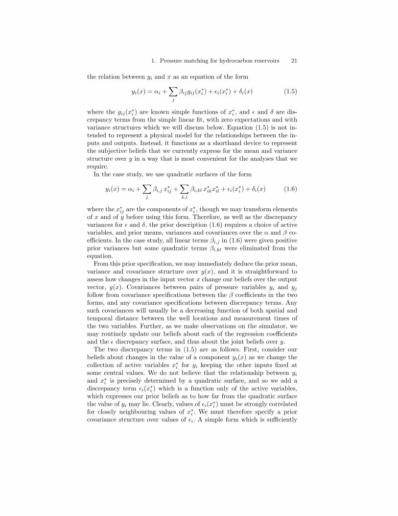
the relation between yi and x as an equation of the form
yi(x) = αi +∑j
βijgij(x∗i ) + εi(x∗i ) + δi(x) (1.5)
where the gij(x∗i ) are known simple functions of x∗i , and ε and δ are dis-crepancy terms from the simple linear fit, with zero expectations and withvariance structures which we will discuss below. Equation (1.5) is not in-tended to represent a physical model for the relationships between the in-puts and outputs. Instead, it functions as a shorthand device to representthe subjective beliefs that we currently express for the mean and variancestructure over y in a way that is most convenient for the analyses that werequire.
In the case study, we use quadratic surfaces of the form
yi(x) = αi +∑j
βi,j x∗ij +
∑k,l
βi,kl x∗ikx∗il + εi(x∗i ) + δi(x) (1.6)
where the x∗ij are the components of x∗i , though we may transform elementsof x and of y before using this form. Therefore, as well as the discrepancyvariances for ε and δ, the prior description (1.6) requires a choice of activevariables, and prior means, variances and covariances over the α and β co-efficients. In the case study, all linear terms βi,j in (1.6) were given positiveprior variances but some quadratic terms βi,kl were eliminated from theequation.
From this prior specification, we may immediately deduce the prior mean,variance and covariance structure over y(x), and it is straightforward toassess how changes in the input vector x change our beliefs over the outputvector, y(x). Covariances between pairs of pressure variables yi and yjfollow from covariance specifications between the β coefficients in the twoforms, and any covariance specifications between discrepancy terms. Anysuch covariances will usually be a decreasing function of both spatial andtemporal distance between the well locations and measurement times ofthe two variables. Further, as we make observations on the simulator, wemay routinely update our beliefs about each of the regression coefficientsand the ε discrepancy surface, and thus about the joint beliefs over y.
The two discrepancy terms in (1.5) are as follows. First, consider ourbeliefs about changes in the value of a component yi(x) as we change thecollection of active variables x∗i for yi keeping the other inputs fixed atsome central values. We do not believe that the relationship between yiand x∗i is precisely determined by a quadratic surface, and so we add adiscrepancy term εi(x∗i ) which is a function only of the active variables,which expresses our prior beliefs as to how far from the quadratic surfacethe value of yi may lie. Clearly, values of εi(x∗i ) must be strongly correlatedfor closely neighbouring values of x∗i . We must therefore specify a priorcovariance structure over values of εi. A simple form which is sufficiently

22 Peter S. Craig, Michael Goldstein, Allan H. Seheult, James A. Smith
flexible to represent all of those aspects of our prior beliefs that we wishedto express is
Cov[εi(x∗i ), εi(x∗′i )] = σ2
εi exp[−θi(x∗i − x∗
′
i )T (x∗i − x∗′
i )]
(1.7)
Secondly, consider our beliefs about changes in the value of a componentyi(x) as we change the whole collection of inputs x. We do not believe thatsuch changes are entirely determined by changes in the active variables, andso we add a second discrepancy term δi(x), to represent our prior beliefsabout variation in yi caused by changes in the whole collection of variables.Careful specification of the covariance structure of beliefs over the values ofδi(x) would again involve some form like (1.7) to express beliefs about localcorrelation. However, at this point we introduce a pragmatic simplification.Each of the other terms in (1.5) involves only the active variables for thecomponent under consideration. It is an enormous simplification for theresulting analysis if we can preserve this property over δi. Therefore, whenwe are updating beliefs over yi(x), we will essentially treat the inputs thatwe have excluded from the active set as unknowns, so that we assign overδi(x) a constant variance σ2
δiand constant covariance (in the case study
this covariance was always set to zero) for any pair of different values ofx. Basic to this simplification is the condition that the extra variation inyi(x) due to variation in elements of x which are excluded from x∗i is smallcompared to variation in yi(x) attributable to variation in x∗i . Provided thatσ2δi
is small, we lose little in our predictive description, while enormouslysimplifying each stage of the ensuing analysis, by this approximation.
The covariance structure for a component yi(x) is therefore determinedby the choice of active variables x∗i , functional forms gij(x∗i ), the quantifi-cation of second order beliefs over the coefficients αi and βij , the choiceof constants in (1.7), and the variance of δi(x). The status of the variouselements in (1.5) is further discussed in [CGSS96]. For our present pur-poses, these forms are simply intended to explain sufficient of the prioruncertainties in the problem to suggest a sensible search strategy for goodhistory matches, while being straightforward enough for this search strat-egy to be tractable. At each stage, these descriptions are provisional, to bemodified according to the results of diagnostic testing, and subsequentlyto be reassessed over sub-regions of the input space which are consideredmost likely to contain acceptable history matches.
7 Prior Specification
We use two sources of information for constructing prior beliefs. First, weuse qualitative and quantitative judgements of reservoir engineers. Sec-ondly, we construct and experiment on fast, approximate versions of the
1. Pressure matching for hydrocarbon reservoirs 23
simulator. These two sources are combined to quantify the prior descrip-tion given in Section 6. We shall outline the basic stages of the process,describing what we now consider to be a sensible sequence of elicitationsteps. This sequence was roughly followed in the case study, but, as thiswas very much a learning process, some of the steps were done in paralleland reconsidered several times in order to obtain a prior description.
7.1 Experts’ Judgements
The first stage in the prior specification was informal discussions with areservoir engineer from SSI who was familiar with the particular reservoir.These discussions clarified basic objectives and identified potential diffi-culties. Informal consideration was given to the qualitative relationshipsbetween inputs and outputs. An initial region of interest was selected asmost likely to contain the reservoir geology, based around a central assess-ment by a geologist as to likely values for the variables.
Resulting from these discussions, we decided to vary two types of quan-tities to match the observed pressures. First, permeability multipliers wereallowed to vary between 0.1 and 10. The variables we use to control thesemultipliers are on a log10 scale, varying from −1 to 1. Secondly, fault trans-missibility multipliers may vary over a range of possible values from 0 (asealing fault, allowing nothing to flow through) to 1 (allowing normal flow),and it was decided to use the whole range. A square root transform of thescale of the fault variable was suggested by subsequent analysis.
We also discussed the magnitudes of the measurement errors as quanti-fied by the prior variances for yE in (1.3). There are three ways in whichpressures at wells may be measured, for each of which a prior precision waselicited, based on 90% intervals for error magnitudes which varied between2% and 10% of observed values. For some of the wells, it was clear that themost accurate method had been used, but, in general, information aboutmeasurement procedures had not been recorded and was not easily avail-able. For some of the readings, inferences could be drawn as to the likelymethod of measurement, but for most a compromise accuracy was chosen.The engineer was happy that the components of yE should be uncorrelatedwith each other and with all other terms.
We further discussed the magnitude of differences between the simulatorand the reservoir, as quantified by the prior variances for yD in (1.4). It be-came clear that beliefs about these differences were based on rather subtleconsiderations. Our impression was that there was substantial prior infor-mation which could have been elicited but that this would have requiredconsiderable modelling. If our primary intention had been to make infer-ences about the composition of the reservoir, then this would have formeda central part of the prior structuring. However, as we were primarily con-cerned with the history match, we restricted attention to simple generalstatements of uncertainty. In particular, the median of the absolute mag-
24 Peter S. Craig, Michael Goldstein, Allan H. Seheult, James A. Smith
nitudes of the percentage changes due to the components of yD was judgedto be 5% of the true values, and correlations between different componentsof yD were largely judged on spatial terms with a correlation of 0.8 at adistance of 200m and negligible correlation at 1600m. However, this wascomplicated by faults: the effective distance between two wells separated byan active fault would be substantially greater than the physical distance,so that generally fault transmissibility should be used to modify physicaldistance.
The reservoir engineer further considered that the correlation structureand expected size of differences between the fast and the full simulatorwould be of a similar order of magnitude to those between the full simulatorand the reservoir.
7.2 Using a Fast Simulator
In order to use (1.6), we need to identify a collection of active input variablesfor each component yi and quantify prior beliefs about the magnitudes ofthe various coefficients in this prior description. This is a difficult and timeconsuming process, which must be repeated for each of a large number ofoutput quantities. Further, we intend to re-examine our choices at certainstages in our search procedure. Therefore, it is very useful to have additionalsources of prior information which we can use in a semi-automatic fashionto simplify the prior specification. For this reason, we constructed a fastversion of the simulator, based on a coarser gridding of the reservoir, whichtook between ten and fifteen minutes per evaluation, as opposed to a fewdays. It was considered that the qualitative features of the two simulatorsmight be sufficiently similar that collections of active variables identifiedon the fast simulator could serve as a choice of active variables in the priordescription of beliefs for the full simulator, and that fitting models of form(1.6) on the fast simulator would give us reasonable prior means for thecorresponding quantities on the full simulator.
We therefore ran the fast version of the simulator many times. In thestudy, we chose a 100 run Latin hypercube design (see [MCB79]) in the 40input variables under consideration. As the study proceeded, we found thatthere was much additional information from the fast simulator results whichcould be exploited, and a larger hypercube might have been preferable.Against this, however, must be weighed the additional use of time andresources. In general, we suggest running a large hypercube at the firststage of the process and rather smaller hypercubes when we subsequentlycome to refit our descriptions over sub-regions.
We now have observations on 100 pairs of input and output vectors. Forsimplicity, we treated each component, yi, of the output vector separately,so that for each component, we had 100 observations of the form (x, yi(x)).These observations were used (i) to select a collection of active input vari-ables for yi, with a separate choice made for each i, (ii) to choose which

1. Pressure matching for hydrocarbon reservoirs 25
quadratic terms to include in addition to the linear terms in the prior de-scription (1.6) and (iii) to aid in quantifying prior beliefs for use with thisprior description on the full simulator.
The process for making the choice, for a given i, is as follows:
1. We first use the stepwise routine in S-PLUS (see [Inc93]) to fit yion linear and quadratic terms in all input variables by using ordinaryleast squares. The first six input variables to enter the description areconsidered as candidate active variables for yi. This was a pragmaticchoice to reduce the computational effort in the next stage of theselection process, but generally we found that there was very littleresidual variability left in each yi by this stage.
2. Now we search stepwise for the ‘best description’ using three or fewerof the six candidate active variables. For each candidate collection ofactive variables, we identify stepwise the best choice of quadratic andinteraction terms to supplement the linear terms in those active vari-ables. The searches require a criterion for selection of active variablesand terms. We considered various criteria for good prior descriptionsin the study, seeking descriptions which are likely to be useful forrestricting the range of possible inputs x for which yi(x) might be anacceptable pressure match. The quantification that was finally usedwas based on selecting the combination of variables which maximised,stepwise, a criterion which is based on the following intuitive moti-vation. Our intention in selecting active input variables is to identify,and therefore eliminate from further consideration, choices of inputswhich are implausible as providing good pressure matches on the fullsimulator. How this will happen is that we will choose sequentiallya set of observations to make on the full simulator, at each stageupdating our mean and variance, for the value of yi(x) for each x,by Bayes linear fitting. As we update our beliefs, we also calculate‘implausibility’ measures, which are intended to identify those col-lections of inputs which may be removed from the starting set R ofpossible input values because according to our adjusted beliefs weshall consider that it is highly ‘implausible’ that these values couldgive an adequate pressure match. Implausibility measures are dis-cussed in Section 8 below. Focussing on component yi, the univariateversions of the measures are based on the magnitude of the followingquantity, which has the important property that it can be calculatedpurely on the basis of first and second-order prior beliefs assigned tothe various quantities, namely
(ED[yi(x)− yTi])2
VarD[yi(x)− yTi]. (1.8)
where yTi is the ith component of yT in (1.3), and the adjusted ex-pectations and variances are taken using (1.1) and (1.2) based on the
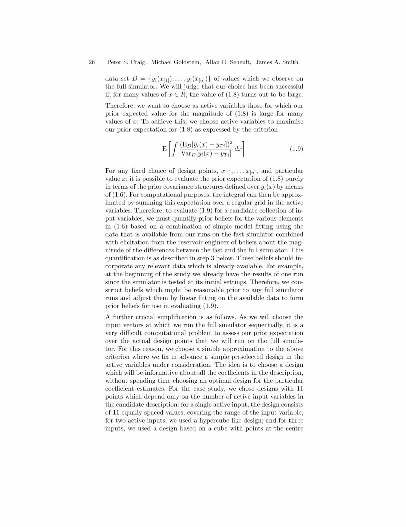
26 Peter S. Craig, Michael Goldstein, Allan H. Seheult, James A. Smith
data set D = {yi(x[1]), . . . , yi(x[n])} of values which we observe onthe full simulator. We will judge that our choice has been successfulif, for many values of x ∈ R, the value of (1.8) turns out to be large.
Therefore, we want to choose as active variables those for which ourprior expected value for the magnitude of (1.8) is large for manyvalues of x. To achieve this, we choose active variables to maximiseour prior expectation for (1.8) as expressed by the criterion
E[∫
(ED[yi(x)− yTi])2
VarD[yi(x)− yTi]dx
](1.9)
For any fixed choice of design points, x[1], . . . , x[n], and particularvalue x, it is possible to evaluate the prior expectation of (1.8) purelyin terms of the prior covariance structures defined over yi(x) by meansof (1.6). For computational purposes, the integral can then be approx-imated by summing this expectation over a regular grid in the activevariables. Therefore, to evaluate (1.9) for a candidate collection of in-put variables, we must quantify prior beliefs for the various elementsin (1.6) based on a combination of simple model fitting using thedata that is available from our runs on the fast simulator combinedwith elicitation from the reservoir engineer of beliefs about the mag-nitude of the differences between the fast and the full simulator. Thisquantification is as described in step 3 below. These beliefs should in-corporate any relevant data which is already available. For example,at the beginning of the study we already have the results of one runsince the simulator is tested at its initial settings. Therefore, we con-struct beliefs which might be reasonable prior to any full simulatorruns and adjust them by linear fitting on the available data to formprior beliefs for use in evaluating (1.9).
A further crucial simplification is as follows. As we will choose theinput vectors at which we run the full simulator sequentially, it is avery difficult computational problem to assess our prior expectationover the actual design points that we will run on the full simula-tor. For this reason, we choose a simple approximation to the abovecriterion where we fix in advance a simple preselected design in theactive variables under consideration. The idea is to choose a designwhich will be informative about all the coefficients in the description,without spending time choosing an optimal design for the particularcoefficient estimates. For the case study, we chose designs with 11points which depend only on the number of active input variables inthe candidate description: for a single active input, the design consistsof 11 equally spaced values, covering the range of the input variable;for two active inputs, we used a hypercube like design; and for threeinputs, we used a design based on a cube with points at the centre
1. Pressure matching for hydrocarbon reservoirs 27
and in the middle of each face and with four other points on verticesof a smaller nested cube.
We have made a variety of somewhat ad hoc choices in order tochoose the preferred collection of active variables. As yet, we havelittle experience as to the sensitivity of our approach to the variousapproximations and assumptions that we have made. However, themethod appeared to select sensible collections of active variables inan automatic fashion in the present study.
3. For each component, yi, we have now selected a collection of threeactive input variables x∗i , and decided which quadratic terms in thesevariables to include in the relation (1.6). The quantification of priorbeliefs over these quantities proceeds as follows. We begin by fit-ting the chosen linear description in the selected variables to the fastsimulator data using ordinary least squares, assuming an uncorre-lated error structure. This is a reasonable approximation, as we havea large sample on a roughly orthogonal design, with values whichare reasonably well separated. The estimated coefficients αi, βi,j andβi,kl are taken to be the corresponding prior means E[αi], E[βi,j ] andE[βi,kl] for the coefficients on the full simulator, and the variance ma-trix of these coefficients is the sum of two components. The first is ouruncertainty about the value of the estimates from the fast simulatorand is taken as the standard estimate from the coefficient variancematrix. The second component represents the engineer’s uncertaintyabout the difference between the two simulators and was taken to bediagonal with each standard deviation for the diagonal taken to be5% of the corresponding coefficient estimate. This was subsequentlyincreased as the case study progressed; see Section 9.
The covariance assessments for εi(x∗i ) and δi(x) are estimated fromthe residuals from the ordinary least squares fit as follows. The over-all error variance, σ2
εi + σ2δi
, is estimated by the residual variance.Individual values for σ2
δiand σ2
εi are found from examining the cor-relations between ‘neighbouring residuals’, as we always treat δi(x)as having zero spatial correlation. As it is hard to estimate θi fromthe data, we chose a value for θi which depended only on the numberof active variables: 85 for one active variable, 42 for two and 32 forthree active variables. This simplification is possible because, for thedescription building process, we linearly transform each input vari-able to the range [−0.5, 0.5]. The chosen values were arrived at byexamination of the spatial autocorrelation function of the residualsfrom quadratic fits to cubic polynomials. Prior covariances betweenany of the four components αi, βi, εi and δi are all zero.
Plots of the spatial and temporal configuration of coefficients for pres-sures yi with the same active variables were then used to assess how much

28 Peter S. Craig, Michael Goldstein, Allan H. Seheult, James A. Smith
spatial and temporal correlation should be built into the prior specification,and to compare with the order of magnitude correlations suggested by thereservoir engineer. There is scope here for more detailed data analysis andmodelling. Overall, we had considerably more confidence in our marginalspecifications than in our joint specification. This, together with variouscomputational problems, led us to prefer marginal to joint analyses in thestudy.
7.3 Checking the prior specification
In Sections 7.1 and 7.2, we have described the basic steps that we followed inconstructing our prior description. The final stage in constructing the priordescription was to check the qualitative and quantitative form of the priorspecification at which we had arrived in consultation with the reservoirengineer. The form of the specification is complicated as there are manyinput quantities related to many output quantities. We created a graphicalelicitation tool which simplified the task of the reservoir engineer, namelychecking that there did not appear to be any substantial flaws in the priorbeliefs that we now expressed.
Our eventual intention is that the elicitation process should become prop-erly interactive, allowing the reservoir engineer to input a priori both quali-tative belief specifications, which may be used to direct our search for activevariables in the fitting stage on the fast simulator (this becomes increasinglyimportant as the number of inputs increases), and also quantitative priorbelief specifications which we may combine with the evaluations on thesimulator in a consistent Bayes linear way. The elicitation tool was there-fore constructed to facilitate this more general approach to elicitation. Thetool that we created could be used: (i) to create and display relationshipsbetween active input variables and the corresponding outputs, basicallyby showing a map of the reservoir on which different inputs and outputscould be displayed and highlighted, where the elements of the display werelinked to tables of variables and to time plots for the measurements; and(ii) to quantify individual aspects of beliefs, offering both graphical meth-ods for expressing uncertainties as to the effects on a pressure output yifrom changing a geology input xj , and also ways of grouping the variablesfor elicitation purposes so that we could use exchangeability arguments toextrapolate uncertainty statements from one quantity to related classes ofquantities. The details of this more general methodology, and a full de-scription as to how the graphical tool functions to support this approach,will be given elsewhere.
Only a small amount of the functionality of the graphical tool was ex-ploited in the case study, but this was sufficient to help the reservoir engi-neer to grasp the qualitative structure of the prior description that we hadassessed, for example by checking features such as whether similar outputquantities were affected by similar active input quantities. The result of

1. Pressure matching for hydrocarbon reservoirs 29
this process was a general agreement as to the choices of active variablecollections that we had made, but surprise as to how few of the fault vari-ables had been included. This was one of the motivations which later ledus to examine carefully the influence of fault variables and which led to asquare root transformation of those variables; see Section 11. The graphicaltool was also used to assess some simple rule of thumb prior quantificationswhich were roughly in accord with the prior description that we had con-structed at the previous stage.
7.4 Details of the Study
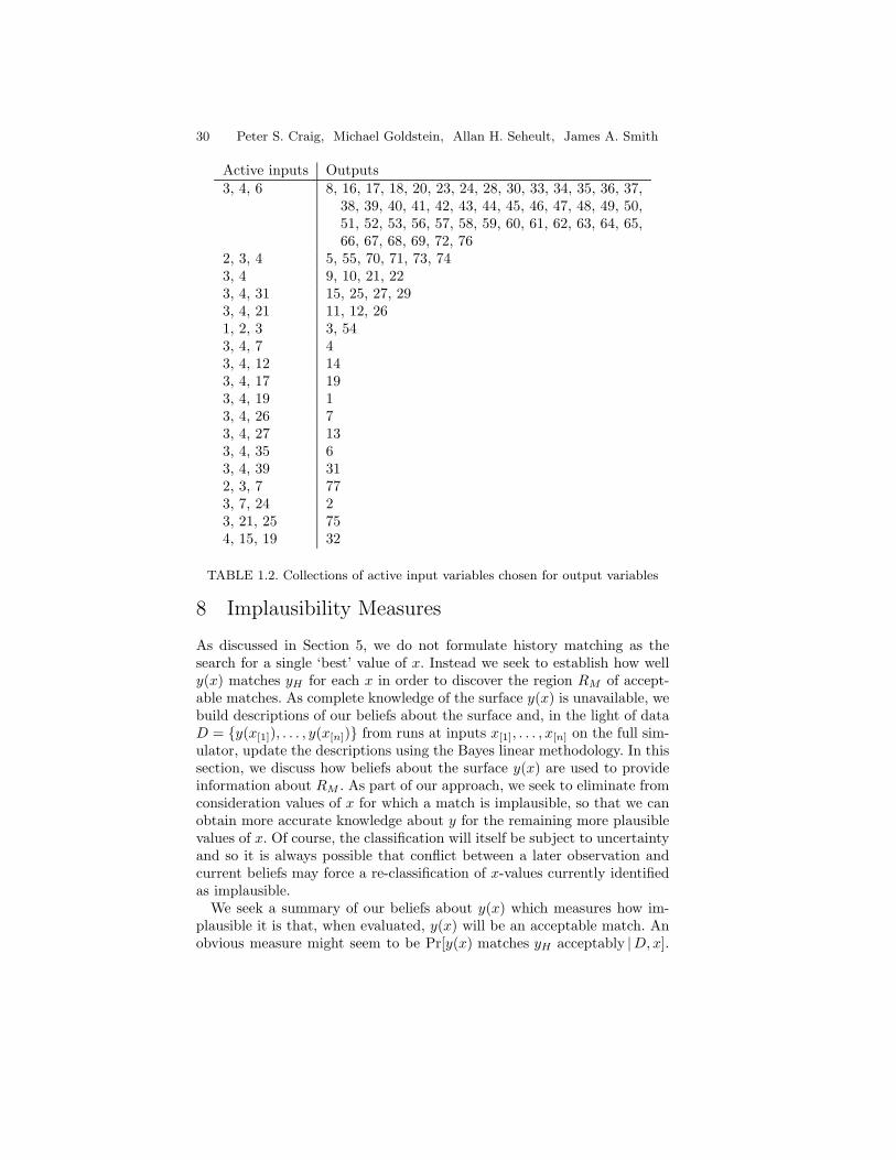
The combinations of active variables chosen are shown in Table 1.2. Recallthat variables 1 to 7 are permeability multipliers for the regions and thatthe remainder are fault transmissibility multipliers. Observe that certaininputs are active for many components; for example, x3, the permeabilitymultiplier for region 3, appears in all but one of the descriptions. By cross-referencing Tables 1.1 and 1.2 and Figures 1 and 2, we can observe that thechoices of active variables seem to be consistent with the physical locationsof wells. For example, the permeability multiplier for region 1 is x1, whichonly appears for outputs at wells in that region. Similarly, outputs fromwells nearer to region 2 are more likely than other outputs to have x2 as anactive variable. The fault transmissibilities which appear as active variablesare usually active for outputs corresponding to wells on which the faultsmight be expected to have an influence.
As an example, the description developed for y9 has two active variables,x3 and x4, each ranging from −1 to 1. The form of the description is
y9(x) = α9 + β9,1x3 + β9,2x4 + β9,12x3x4 + ε9(x3, x4) + δ9(x)
The estimated values of σε9 and σδ9 are respectively 41 and 11. Havingadjusted by the data from running the simulator at its initial settings, themeans for α9, β9,1, β9,2 and β9,12 are respectively 2029, 213, 121 and 80.The corresponding standard deviations are 38, 13, 10 and 13. All coefficientcorrelations are negligible, the largest magnitude being 0.04.
Examination of the means of coefficients of x3 and x4 in all of thesedescriptions showed clear spatial and chronological structure. There wasstrong evidence that for wells in region 4 (the vast majority), the time ofmeasurement could be used to help predict the coefficients. There was alsoclear evidence that the wells in regions 1, 2 and 3 behave differently fromthose in region 4, and that those in region 5 differ from both groups. Onthis basis, supported by the beliefs of the reservoir engineer, we decided toorganise the y-variables into 12 groups, splitting them by time of measure-ment and by region of the reservoir in which the well is located (see column5 of Table 1.1).
30 Peter S. Craig, Michael Goldstein, Allan H. Seheult, James A. Smith
Active inputs Outputs3, 4, 6 8, 16, 17, 18, 20, 23, 24, 28, 30, 33, 34, 35, 36, 37,
38, 39, 40, 41, 42, 43, 44, 45, 46, 47, 48, 49, 50,51, 52, 53, 56, 57, 58, 59, 60, 61, 62, 63, 64, 65,66, 67, 68, 69, 72, 76
2, 3, 4 5, 55, 70, 71, 73, 743, 4 9, 10, 21, 223, 4, 31 15, 25, 27, 293, 4, 21 11, 12, 261, 2, 3 3, 543, 4, 7 43, 4, 12 143, 4, 17 193, 4, 19 13, 4, 26 73, 4, 27 133, 4, 35 63, 4, 39 312, 3, 7 773, 7, 24 23, 21, 25 754, 15, 19 32
TABLE 1.2. Collections of active input variables chosen for output variables
8 Implausibility Measures
As discussed in Section 5, we do not formulate history matching as thesearch for a single ‘best’ value of x. Instead we seek to establish how welly(x) matches yH for each x in order to discover the region RM of accept-able matches. As complete knowledge of the surface y(x) is unavailable, webuild descriptions of our beliefs about the surface and, in the light of dataD = {y(x[1]), . . . , y(x[n])} from runs at inputs x[1], . . . , x[n] on the full sim-ulator, update the descriptions using the Bayes linear methodology. In thissection, we discuss how beliefs about the surface y(x) are used to provideinformation about RM . As part of our approach, we seek to eliminate fromconsideration values of x for which a match is implausible, so that we canobtain more accurate knowledge about y for the remaining more plausiblevalues of x. Of course, the classification will itself be subject to uncertaintyand so it is always possible that conflict between a later observation andcurrent beliefs may force a re-classification of x-values currently identifiedas implausible.
We seek a summary of our beliefs about y(x) which measures how im-plausible it is that, when evaluated, y(x) will be an acceptable match. Anobvious measure might seem to be Pr[y(x) matches yH acceptably |D,x].
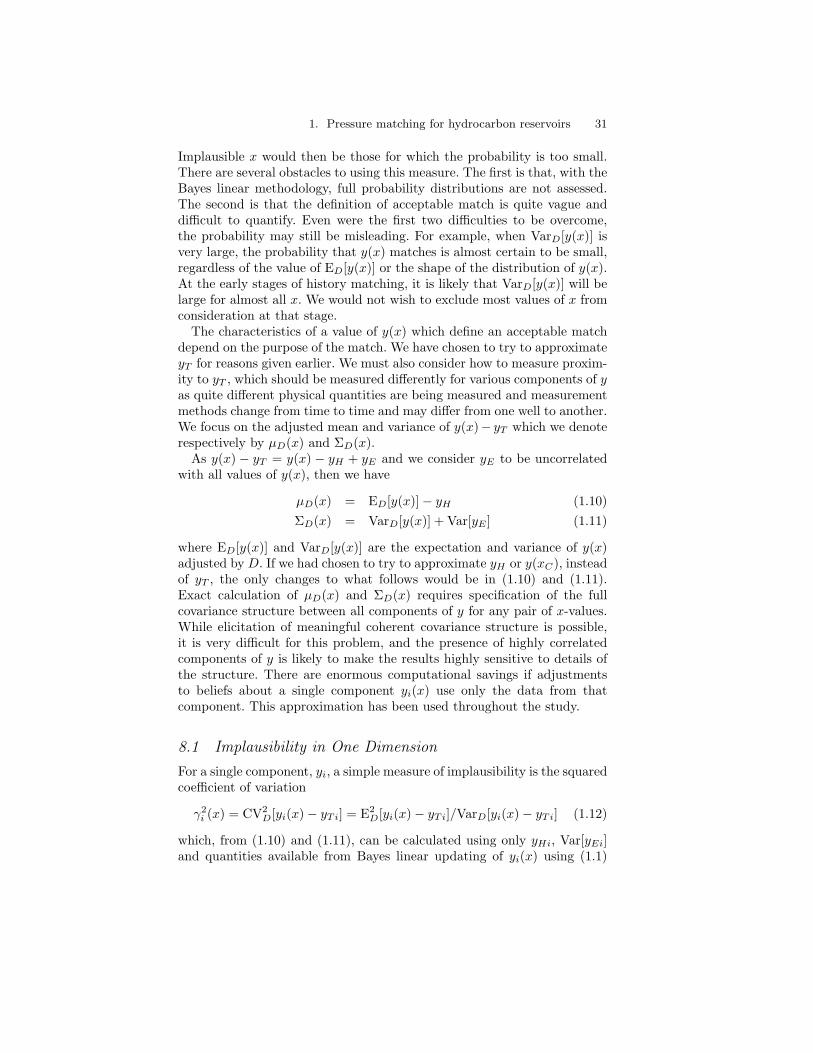
1. Pressure matching for hydrocarbon reservoirs 31
Implausible x would then be those for which the probability is too small.There are several obstacles to using this measure. The first is that, with theBayes linear methodology, full probability distributions are not assessed.The second is that the definition of acceptable match is quite vague anddifficult to quantify. Even were the first two difficulties to be overcome,the probability may still be misleading. For example, when VarD[y(x)] isvery large, the probability that y(x) matches is almost certain to be small,regardless of the value of ED[y(x)] or the shape of the distribution of y(x).At the early stages of history matching, it is likely that VarD[y(x)] will belarge for almost all x. We would not wish to exclude most values of x fromconsideration at that stage.
The characteristics of a value of y(x) which define an acceptable matchdepend on the purpose of the match. We have chosen to try to approximateyT for reasons given earlier. We must also consider how to measure proxim-ity to yT , which should be measured differently for various components of yas quite different physical quantities are being measured and measurementmethods change from time to time and may differ from one well to another.We focus on the adjusted mean and variance of y(x)− yT which we denoterespectively by µD(x) and ΣD(x).
As y(x) − yT = y(x) − yH + yE and we consider yE to be uncorrelatedwith all values of y(x), then we have
µD(x) = ED[y(x)]− yH (1.10)ΣD(x) = VarD[y(x)] + Var[yE ] (1.11)
where ED[y(x)] and VarD[y(x)] are the expectation and variance of y(x)adjusted by D. If we had chosen to try to approximate yH or y(xC), insteadof yT , the only changes to what follows would be in (1.10) and (1.11).Exact calculation of µD(x) and ΣD(x) requires specification of the fullcovariance structure between all components of y for any pair of x-values.While elicitation of meaningful coherent covariance structure is possible,it is very difficult for this problem, and the presence of highly correlatedcomponents of y is likely to make the results highly sensitive to details ofthe structure. There are enormous computational savings if adjustmentsto beliefs about a single component yi(x) use only the data from thatcomponent. This approximation has been used throughout the study.
8.1 Implausibility in One Dimension
For a single component, yi, a simple measure of implausibility is the squaredcoefficient of variation
γ2i (x) = CV2
D[yi(x)− yTi] = E2D[yi(x)− yTi]/VarD[yi(x)− yTi] (1.12)
which, from (1.10) and (1.11), can be calculated using only yHi, Var[yEi]and quantities available from Bayes linear updating of yi(x) using (1.1)
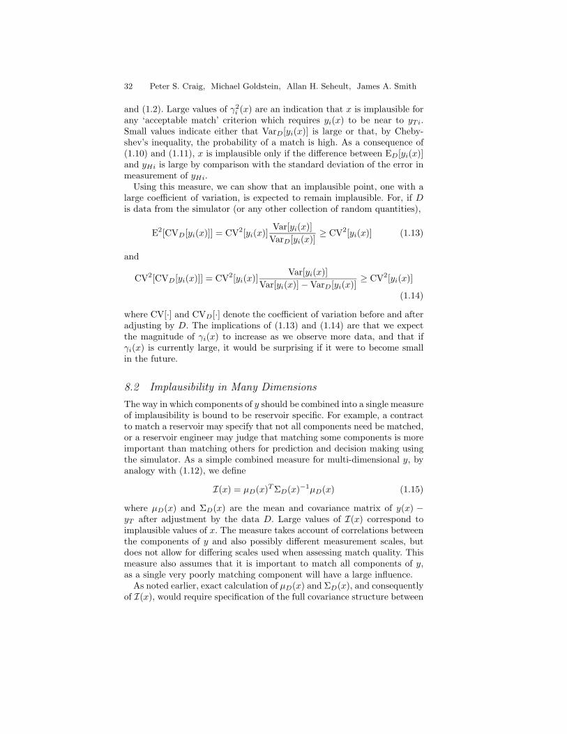
32 Peter S. Craig, Michael Goldstein, Allan H. Seheult, James A. Smith
and (1.2). Large values of γ2i (x) are an indication that x is implausible for
any ‘acceptable match’ criterion which requires yi(x) to be near to yTi.Small values indicate either that VarD[yi(x)] is large or that, by Cheby-shev’s inequality, the probability of a match is high. As a consequence of(1.10) and (1.11), x is implausible only if the difference between ED[yi(x)]and yHi is large by comparison with the standard deviation of the error inmeasurement of yHi.
Using this measure, we can show that an implausible point, one with alarge coefficient of variation, is expected to remain implausible. For, if Dis data from the simulator (or any other collection of random quantities),
E2[CVD[yi(x)]] = CV2[yi(x)]Var[yi(x)]
VarD[yi(x)]≥ CV2[yi(x)] (1.13)
and
CV2[CVD[yi(x)]] = CV2[yi(x)]Var[yi(x)]
Var[yi(x)]−VarD[yi(x)]≥ CV2[yi(x)]
(1.14)
where CV[·] and CVD[·] denote the coefficient of variation before and afteradjusting by D. The implications of (1.13) and (1.14) are that we expectthe magnitude of γi(x) to increase as we observe more data, and that ifγi(x) is currently large, it would be surprising if it were to become smallin the future.
8.2 Implausibility in Many Dimensions
The way in which components of y should be combined into a single measureof implausibility is bound to be reservoir specific. For example, a contractto match a reservoir may specify that not all components need be matched,or a reservoir engineer may judge that matching some components is moreimportant than matching others for prediction and decision making usingthe simulator. As a simple combined measure for multi-dimensional y, byanalogy with (1.12), we define
I(x) = µD(x)TΣD(x)−1µD(x) (1.15)
where µD(x) and ΣD(x) are the mean and covariance matrix of y(x) −yT after adjustment by the data D. Large values of I(x) correspond toimplausible values of x. The measure takes account of correlations betweenthe components of y and also possibly different measurement scales, butdoes not allow for differing scales used when assessing match quality. Thismeasure also assumes that it is important to match all components of y,as a single very poorly matching component will have a large influence.
As noted earlier, exact calculation of µD(x) and ΣD(x), and consequentlyof I(x), would require specification of the full covariance structure between

1. Pressure matching for hydrocarbon reservoirs 33
all components of y for any pair of x-values. We have chosen in this study touse approximations to I(x) which do not use the full covariance structureand which greatly reduce the computational burden. There are a number ofreasons why computation is made quicker by not using the full correlationstructure of y(x). First, adjustment calculations can be carried out sepa-rately for each component of y, using only data from the same component,which immediately reduces the size of covariance matrices used by a factorof p2 (5929 in the case study). Secondly, each component implausibility γiis a function of at most three components of x, which makes it possible tocalculate γi on a grid of x-values. Thirdly, the forms of the approximationsto I(x) allow further computational savings to be described in Section 8.5.
Let us note two extreme situations in which I(x) takes simple forms.If the components of y are uncorrelated, then I(x) =
∑i γ
2i (x) where
γ2i (x), the ‘marginal’ implausibility of x based on component yi, is the
coefficient of variation of yi(x) − yTi, as in (1.12). On the other hand, ifthe p components of y are perfectly correlated then, using a generalisedinverse of ΣD, the implausibility is I(x) = 1
p
∑i γ
2i (x). In both cases, the
adjustments required to compute γi use only the simulator data for thei-th component.
In order to approximate I(x), we divide the components of y into mu-tually exclusive subsets, which are chosen so that the subsets are judgedto be nearly uncorrelated and so that, within each subset, the componentsare judged to be strongly correlated. Consequently, we sum implausibilitiesarising from each of the subsets where the implausibility for each subset isthe average of the corresponding ‘marginal’ implausibilities. Denoting thesubsets by S1, S2, . . . , we approximate I(x) by
I(x) =∑j
1|Sj |
∑i∈Sj
γ2i (x) (1.16)
where |Sj | denotes the number of components of y in Sj . This measurecombines implausibilities associated with the individual components of yin a way which reflects to some extent our beliefs about their correlations.
A quite different measure also used in the case study is
I(x) = maxi|γi(x)| (1.17)
which is conservative, as it is based on the important requirement to only‘rule in’ those inputs which may give an acceptable match for all compo-nents; that is, a point is implausible if it is implausible for at least onecomponent of y. As before, if we ignore the correlation structure of y, wecompute γi using only data values for yi and we obtain the same compu-tational savings as with I(x). A less sensitive measure might be the m-thlargest value of |γi| which, used to define implausibility, would mean thatimplausible values of x were those for which at least m components of y

34 Peter S. Craig, Michael Goldstein, Allan H. Seheult, James A. Smith
failed to match. We have not used it in this study because the computationswould become rather more complex.
Whatever measure of implausibility we choose, the notion appears manytimes in our overall methodology: (i) to help remove from considerationimplausible subsets of x values; (ii) to guide the choice of x-values forruns of the full simulator as described in Section 10, the idea being tochoose as input the value of x whose y will most reduce overall uncertaintyabout y-values for the set of plausible x; (iii) as part of the process ofchoosing descriptions for the components of y, in Section 6; and (iv) toassist informally in deciding when to reformulate the description on a newsub-region of input values.
8.3 Presentation and Interpretation of Implausibility
The implausibility criteria described are functions of all of the componentsof x. For presentation and interpretation, we need to assess implausibilityfor small subsets of the components of x. It seems reasonable that a value ofa single component of x is implausible only if it is implausible for all possiblevalues of the other components. Hence, if x′ and x′′ are complementarysubsets of the components of x, we consider, as a measure of implausibilityfor the components in x′, the projection
minx′′I(x) (1.18)
which is a function only of x′. We can project I(x) and I(x) in the sameway.
Other methods for projecting implausibility measures are possible. How-ever, in the case study, we have used only the method in (1.18), projectingonto at most three components and very often just two, to aid in the visu-alisation of implausibility.
As a basis for assessing implausibility based solely on our restricted beliefspecification we use an heuristic based on the ‘three sigma rule’ [Puk94],which states that for any continuous unimodal density at least 95% of theprobability is within 3 standard deviations of the mean. This informallysuggests that for a single component a value of γ2
i ≥ 9 corresponds to inputwhich is implausible as a match. As a rough calibration for I(x) in (1.16) wehave informally compared values to quantiles of a χ2 distribution having thesame number of degrees of freedom as there are groups, informally treatingthe groups as independent. We treat I(x) from (1.17) as a confirmatorycheck that plausibilities are similar for both plausibility methods.
There are potential dangers associated with the use of either (1.15) or(1.17). In the former, there is the danger that by combining plausibilitycontributions of the components of y through the generalised coefficient ofvariation, we may miss anomalous components or conflicts between groupsof components, which also may make meaningless the overall measure of
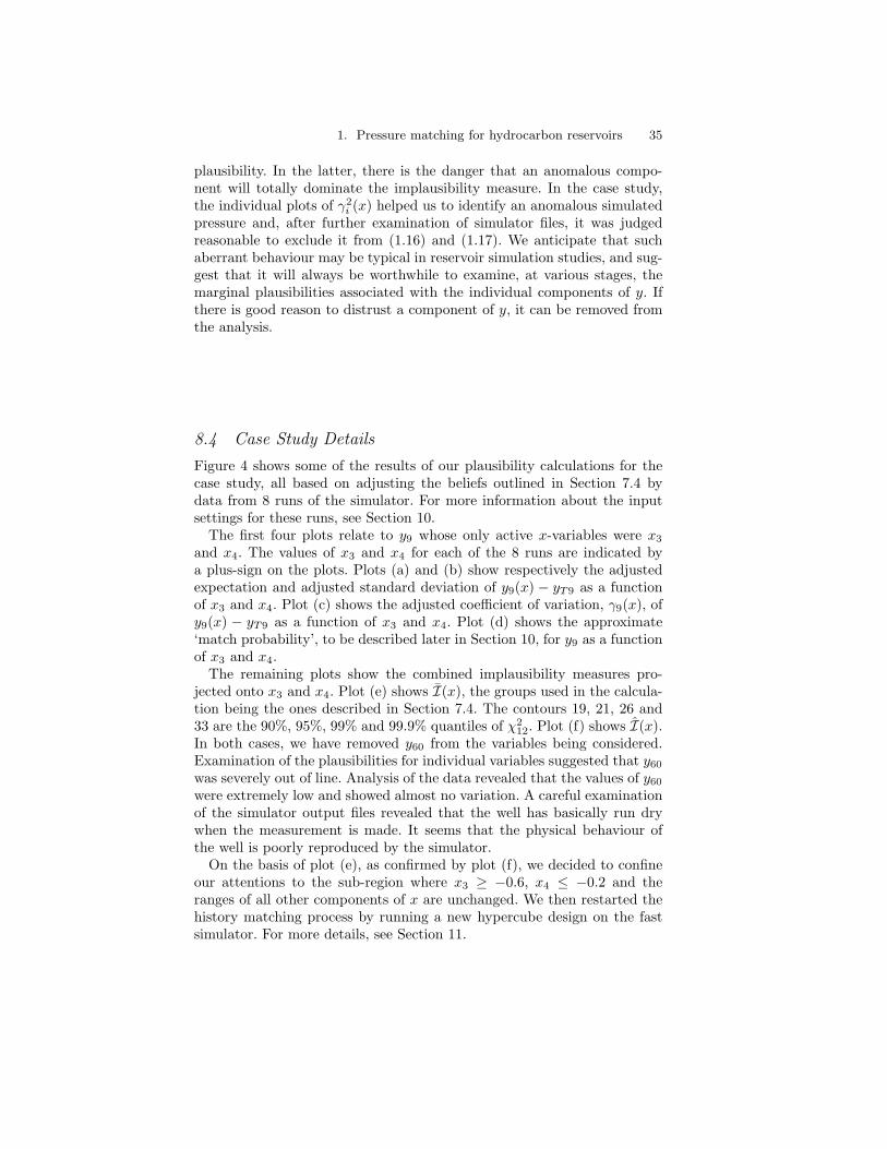
1. Pressure matching for hydrocarbon reservoirs 35
plausibility. In the latter, there is the danger that an anomalous compo-nent will totally dominate the implausibility measure. In the case study,the individual plots of γ2
i (x) helped us to identify an anomalous simulatedpressure and, after further examination of simulator files, it was judgedreasonable to exclude it from (1.16) and (1.17). We anticipate that suchaberrant behaviour may be typical in reservoir simulation studies, and sug-gest that it will always be worthwhile to examine, at various stages, themarginal plausibilities associated with the individual components of y. Ifthere is good reason to distrust a component of y, it can be removed fromthe analysis.
8.4 Case Study Details
Figure 4 shows some of the results of our plausibility calculations for thecase study, all based on adjusting the beliefs outlined in Section 7.4 bydata from 8 runs of the simulator. For more information about the inputsettings for these runs, see Section 10.
The first four plots relate to y9 whose only active x-variables were x3
and x4. The values of x3 and x4 for each of the 8 runs are indicated bya plus-sign on the plots. Plots (a) and (b) show respectively the adjustedexpectation and adjusted standard deviation of y9(x) − yT9 as a functionof x3 and x4. Plot (c) shows the adjusted coefficient of variation, γ9(x), ofy9(x) − yT9 as a function of x3 and x4. Plot (d) shows the approximate‘match probability’, to be described later in Section 10, for y9 as a functionof x3 and x4.
The remaining plots show the combined implausibility measures pro-jected onto x3 and x4. Plot (e) shows I(x), the groups used in the calcula-tion being the ones described in Section 7.4. The contours 19, 21, 26 and33 are the 90%, 95%, 99% and 99.9% quantiles of χ2
12. Plot (f) shows I(x).In both cases, we have removed y60 from the variables being considered.Examination of the plausibilities for individual variables suggested that y60
was severely out of line. Analysis of the data revealed that the values of y60
were extremely low and showed almost no variation. A careful examinationof the simulator output files revealed that the well has basically run drywhen the measurement is made. It seems that the physical behaviour ofthe well is poorly reproduced by the simulator.
On the basis of plot (e), as confirmed by plot (f), we decided to confineour attentions to the sub-region where x3 ≥ −0.6, x4 ≤ −0.2 and theranges of all other components of x are unchanged. We then restarted thehistory matching process by running a new hypercube design on the fastsimulator. For more details, see Section 11.

36 Peter S. Craig, Michael Goldstein, Allan H. Seheult, James A. Smith
x3�
x4
-1.0 -0.5 0.0�
0.5�
1.0
-1.0
-0.5
0.0
0.5
1.0
0
0
100
200�
300�
400�
500�
+
+
+
+
+
+
+
+
x3�
x4
-1.0 -0.5 0.0�
0.5�
1.0
-1.0
-0.5
0.0
0.5
1.0
60�
60�
65�
65�
65�
65�
65�
65�
65�
70�
70�
70�
70�
70�
70�
70�
75�
75�
75�
75�
+
+
+
+
+
+
+
+
(a) (b)
x3�
x4
-1.0 -0.5 0.0�
0.5�
1.0
-1.0
-0.5
0.0
0.5
1.0
-1 -0.5 0
0
0.5�
1 1.5
1.5
2�
2.5�
3�
3.5�
4�
4.5�
5�5.5
�
6�
6.5�
+
+
+
+
+
+
+
+
x3�
x4
-1.0 -0.5 0.0�
0.5�
1.0
-1.0
-0.5
0.0
0.5
1.0
0.0001�
0.001�
0.001�
0.01�
0.05�
0.1�
0.5�0.8
�0.8�
0.9�
0.9�
0.95�
0.95�0.99
�0.99
�
+
+
+
+
+
+
+
+
(c) (d)
x3�
x4
-1.0 -0.5 0.0�
0.5�
1.0
-1.0
-0.5
0.0
0.5
1.0
19 1921�26
�33�40
�50�
50�
75�
75�
100
100
150
150
200�
+
+
+
+
+
+
+
+
x3�
x4
-1.0 -0.5 0.0�
0.5�
1.0
-1.0
-0.5
0.0
0.5
1.0
5�
6�
6�
7�
7�
8�
8�
9�
9�
10
10
11
12
+
+
+
+
+
+
+
+
(e) (f)
FIGURE 4. Implausibility related contour plots after 8 runs of the full simulator:(a) expectation of y9(x)−yT9; (b) standard deviation of y9(x)−yT9; (c) coefficientof variation, γ9, of y9(x) − yT9; (d) ‘match probability’ for y9 (see Section 10);(e) I(x) projected onto x3 and x4; (f) I(x) projected onto x3 and x4.

1. Pressure matching for hydrocarbon reservoirs 37
8.5 Computational Details
In this section we discuss how to compute and project our implausibilitymeasures. Presentation in two or three dimensions requires that grids ofvalues of a projected measure are available. A naive approach would requirethe calculation of grids in d dimensions followed by projection. However, dis likely to be large (40 for the case study) and the smallest possible gridrequires 2d values. A fortunate consequence of the model structure in (1.5)together with the forms of the implausibility measures (1.16) and (1.17)and the projection (1.18) is that the computations can be done easily andrapidly subject to one small assumption, namely that we never considera value of x which is the same as any of those at which we have alreadyevaluated y. Under this assumption, the updated values of γ2
i (x) dependonly on the active components of x for yi.
Since we have at most three active components of x for each yi, it isstraightforward to evaluate γ2
i (x) on a regular lattice of points in the activecomponents. In practice, we have used grids having 11 evenly spaced valuesfor each active component. We now need a way to obtain projections of thecombined measures onto a grid of values in a subset of the components ofx. Suppose we want to eliminate xi from the collection:
• If xi appears as an active variable in only a single component of y,then we simply eliminate xi from that component of y by finding theminimum on the grid for each value of xi. The result is a grid in theremaining active components, and we can easily eliminate all thosecomponents of x which appear just once as active components.
• If xi appears as an active variable in more than one component ofy and all share the same set of active components of x, we combinethese components onto a single grid, either by taking the maximumacross the components for each point on the grid or by summing thecomponents (assuming the γ2
i values have already been pre-scaled todo the weighting required for the combined measure) for each pointon the grid. We then replace the original group of components of yby a single virtual component of y with the new grid of values. Nowxi appears as an active variable in just one component, and we canproceed as in the previous item.
• If xi appears as an active component in more than one component ofy and those components do not all have the same active componentsof x, we must first put each of those components of y onto a largergrid corresponding to the joint collection of all components of x whichare active for those components of y under consideration, so that theyeffectively all share the same collection of active components of x. Wethen proceed as in the previous item.
Eliminating one component of x at a time in this manner will lead to the

38 Peter S. Craig, Michael Goldstein, Allan H. Seheult, James A. Smith
required projection. The only danger is that when putting a group of com-ponents of y onto a common grid in the collection of all their active com-ponents of x, we may be creating an unacceptably large grid, making com-putation infeasible. This situation may not always be avoidable. However,it has not been a problem for the case study and eliminating componentsof x in a sensible order should minimise the likelihood of trouble. We havetwo rules: (i) we prefer to eliminate a component which appears rarely asan active component than to eliminate one which appears frequently; and(ii) since it is simple to find what dimension of grid is required to combinea collection of components of y, we always calculate the dimension and,if it is bigger than three, we seek a different component of x to eliminatewhich would require a lower dimensional grid.
We may subsequently wish to find the value on the full d-dimensionalgrid which corresponds to a particular value in a low dimensional projec-tion. This calculation can be done very easily by back-tracking through theprojection process. All that is required is to store the intermediate gridsformed when components of y are being combined during the projectionprocess.
9 Diagnostics
As our prior description is a simplification of an extremely complex pro-cess, we may expect gross discrepancies in certain aspects of our descrip-tion. Therefore, it is important to carry out diagnostic monitoring, so thatwe become aware of conflicts between observed simulator output and ourdescription of beliefs about y(x). A potential conflict arises when some-thing occurs which, a priori, was considered to be very unlikely. Were weusing Bayes theorem to update beliefs, the degree of conflict would be mea-sured by calculating a suitable probability. Bayes linear analyses must usea different kind of diagnostic measure.
Instead of the probability of some chosen event, we measure the sizeof some chosen quantity, Z, by standardising it using its prior mean andstandard deviation to obtain the diagnostic quantity (Z −E[Z])/Var[Z]1/2
which we denote by S[Z]. The prior mean and standard deviation of S[Z]are respectively 0 and 1. Note that the prior beliefs used to calculate S[Z]are not necessarily the initial beliefs but can be those from any subse-quent belief adjustment prior to the observation of Z. Good candidatesfor diagnostic monitoring include observations and beliefs about importantcomponents used to structure beliefs.
As before, suppose that we sequentially observe the simulator outputsy(x[1]), . . . , y(x[n]). We denote the collection of the first j observations byDj = {y(x[1]), . . . , y(x[j])}. To simplify notation, for any random quantityZ, we write Ej [Z] for the adjusted expectation, EDj [Z], of Z given ob-
1. Pressure matching for hydrocarbon reservoirs 39
servations Dj and Varj [Z] for the adjusted variance VarDj [Z]. When weevaluate y(x[j]) on the simulator, we compare the prior expectation with theobserved value. We will mainly be concerned with monitoring changes inindividual components of y, and we denote the value of yi(x[j]) as yij . Notethat, for the purposes of calculating diagnostics, we will treat x[1], x[2], . . .as known. Even if it were interesting to treat them as unknown, the proper-ties of the sequential design process would be extremely difficult to analyse.
We judge discrepancies in an informal manner. For example, we mightconsider that magnitudes of S[yij ] larger than 3 are suggestive of conflictsbetween our prior formulation and the data. However, the general patternsthat emerge from the collection of evaluations are of principal interest,rather than any particular evaluation. For example, large values associatedwith all the pressures at a particular well might suggest that the fast simu-lator poorly approximates the behaviour of the full simulator at that well.Alternatively, occurrence of many very small values for all components of ywould also be important in suggesting that we might have over-inflated theprior uncertainties, for example by over-estimating the differences betweenthe fast and the full simulators.
We may make a more detailed assessment by monitoring the one stepchanges in expectation, E[r/][Z] = Er[Z] − Er−1[Z], of a quantity Z andassessing their standardised values S[r/][Z] = E[r/][Z]/Varr−1[Z]1/2 to iden-tify whether the sequence of changes in the predictions for Z is behavingas we expect. Of particular interest is the standardised one step compar-ison between an observation and its prediction given all of the precedingobservations, namely
S[j/][yij ] =yij − Ej−1[yij ]√
Varj−1[yij ](1.19)
The discrepancy measures S[r/][yij ] compare changes in observation orexpectation to the expected magnitudes of such changes. Thus, a changein belief, although small, may correspond to a large standardised value andbe of diagnostic interest and a large change of belief may correspond to asmall standardised value and have no diagnostic implication. In order toform a qualitative picture as to the nature of the changes between prior andadjusted expectations, we may decompose the collection of changes in beliefas yij − E[yij ] =
∑jr=1 E[r/][yij ], where the terms E[r/][yij ] are mutually
uncorrelated so that Var[yij ] =∑jr=1 Varr−1[E[r/][yij ]]. Therefore, we may
write S[yij ] as
S[yij ] =∑jr=1 E[r/][yij ]√∑j
r=1 Varr−1[E[r/][yij ]].
Thus, if S[yij ] is large, we may identify which terms E[r/][yij ] explain thisapparent discrepancy, while if S[yij ] is small, we can check as to whether

40 Peter S. Craig, Michael Goldstein, Allan H. Seheult, James A. Smith
this is because each term E[r/][yij ] is small, or whether some of the changesare surprisingly large and positive and some similarly negative leading toan apparently moderate standardised value.
Note that while there is a natural time ordering of the simulator runs, wemay still choose to consider stepwise diagnostics based on rearrangementsof the order of the runs, to see how well each observation that we havemade can be predicted by all of the remaining observations.
There are various further diagnostics that we may evaluate. First, ifwe also evaluate the value of y(x) on the fast simulator, giving a valuey′(x), say, then we can evaluate the standardised differences S[yij − y′ij ].Secondly, we can evaluate diagnostics on the revised assessments of thevarious coefficients in the description (1.5), for example evaluating
S[ED[βij ]] =ED[βij ]− E[βij ]√
Var[ED[βij ]](1.20)
where for simplicity we compare overall changes between prior and adjustedexpectations, but we might also examine stepwise changes in these values.
We have concentrated in our account on diagnostics for individual quan-tities as these are simple to evaluate and interpret. There is no difficulty,in principle, in evaluating joint diagnostics. For example, the analogousquantity to S[yij ] for assessing the full observation y(x[j]) is
S[y(x[j])] = (y(x[j])− E[y(x[j])])T (Var[y(x[j])])−1(y(x[j])− E[y(x[j])])
with a similar stepwise decomposition for changes in expectation for y(x[j]).However, in this study, we considered that our joint prior specificationfor the components of y(x) was not sufficiently detailed to merit carefuldiagnostic examination, and thus preferred to concentrate our attention onthe marginal diagnostics, which are also more easily computed.
9.1 Case Study Details
Figure 5 shows boxplots of the standardised one-step ahead comparisons(1.19) for the first 8 runs of the simulator. Each boxplot corresponds to the77 comparisons from a single run. We see that there are large standardisedcomparisons for all runs except the last one. The last run is extremely closein x3 and x4 to a preceding run and since x3 and x4 are very much the mostimportant x-variables, it is hardly surprising that the diagnostics shouldbe much smaller for what is almost a repeated measurement. Rearrangingthe order of runs so that in turn each run is taken as the last run does notgreatly change the sizes of the standardised comparisons.
We suspected that the problem was caused by having under-estimatedthe difference between the full and fast simulators when building our priordescription. The standard deviation of the difference between full and fast
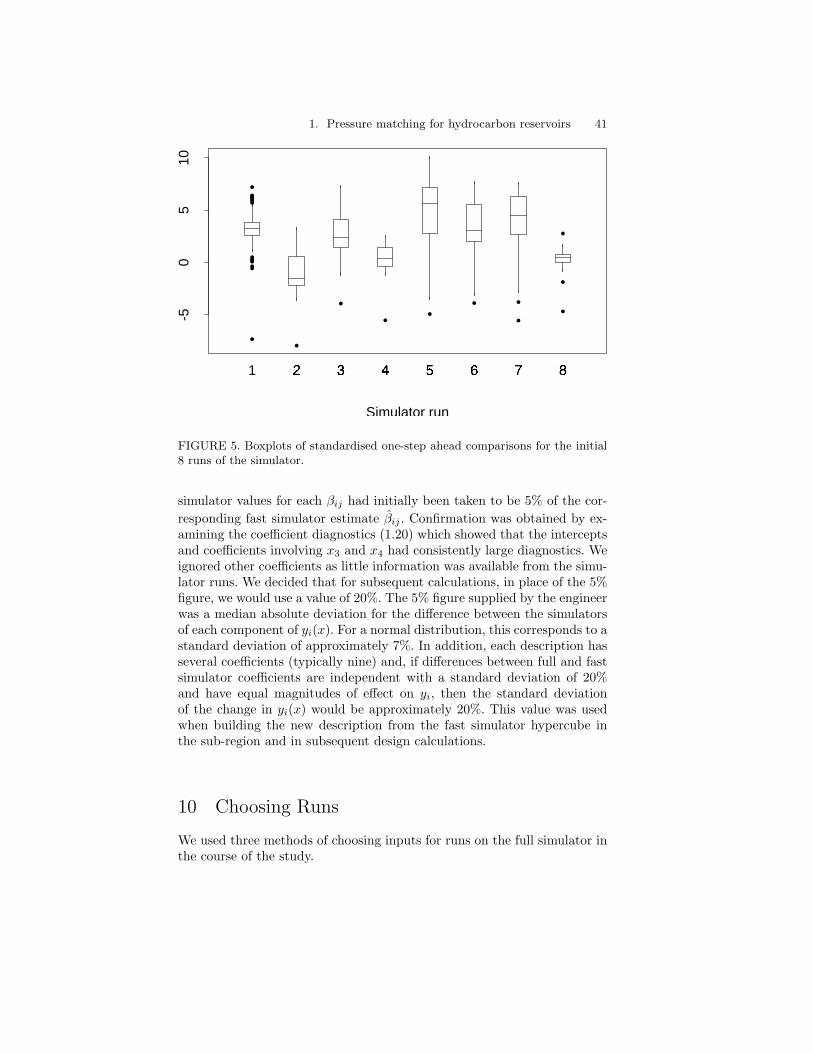
1. Pressure matching for hydrocarbon reservoirs 41
-50
510
•
•••••••
•••••••••
•
•• •
•••
•
•
•
1 2�
3�
4�
5�
6�
7�
8�
Simulator run
FIGURE 5. Boxplots of standardised one-step ahead comparisons for the initial8 runs of the simulator.
simulator values for each βij had initially been taken to be 5% of the cor-responding fast simulator estimate βij . Confirmation was obtained by ex-amining the coefficient diagnostics (1.20) which showed that the interceptsand coefficients involving x3 and x4 had consistently large diagnostics. Weignored other coefficients as little information was available from the simu-lator runs. We decided that for subsequent calculations, in place of the 5%figure, we would use a value of 20%. The 5% figure supplied by the engineerwas a median absolute deviation for the difference between the simulatorsof each component of yi(x). For a normal distribution, this corresponds to astandard deviation of approximately 7%. In addition, each description hasseveral coefficients (typically nine) and, if differences between full and fastsimulator coefficients are independent with a standard deviation of 20%and have equal magnitudes of effect on yi, then the standard deviationof the change in yi(x) would be approximately 20%. This value was usedwhen building the new description from the fast simulator hypercube inthe sub-region and in subsequent design calculations.
10 Choosing Runs
We used three methods of choosing inputs for runs on the full simulator inthe course of the study.
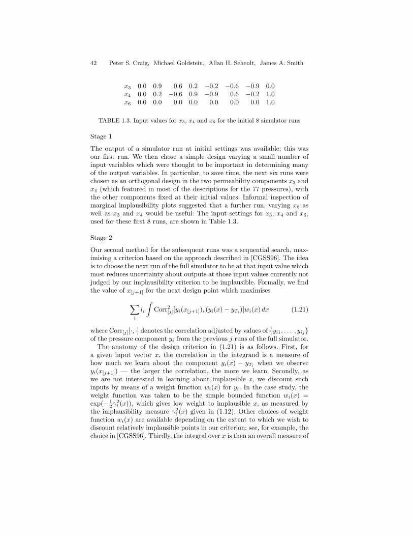
42 Peter S. Craig, Michael Goldstein, Allan H. Seheult, James A. Smith
x3 0.0 0.9 0.6 0.2 −0.2 −0.6 −0.9 0.0x4 0.0 0.2 −0.6 0.9 −0.9 0.6 −0.2 1.0x6 0.0 0.0 0.0 0.0 0.0 0.0 0.0 1.0
TABLE 1.3. Input values for x3, x4 and x6 for the initial 8 simulator runs
Stage 1
The output of a simulator run at initial settings was available; this wasour first run. We then chose a simple design varying a small number ofinput variables which were thought to be important in determining manyof the output variables. In particular, to save time, the next six runs werechosen as an orthogonal design in the two permeability components x3 andx4 (which featured in most of the descriptions for the 77 pressures), withthe other components fixed at their initial values. Informal inspection ofmarginal implausibility plots suggested that a further run, varying x6 aswell as x3 and x4 would be useful. The input settings for x3, x4 and x6,used for these first 8 runs, are shown in Table 1.3.
Stage 2
Our second method for the subsequent runs was a sequential search, max-imising a criterion based on the approach described in [CGSS96]. The ideais to choose the next run of the full simulator to be at that input value whichmost reduces uncertainty about outputs at those input values currently notjudged by our implausibility criterion to be implausible. Formally, we findthe value of x[j+1] for the next design point which maximises
∑i
li
∫Corr2
[j][yi(x[j+1]), (yi(x)− yTi)]wi(x) dx (1.21)
where Corr[j][·, ·] denotes the correlation adjusted by values of {yi1, . . . , yij}of the pressure component yi from the previous j runs of the full simulator.
The anatomy of the design criterion in (1.21) is as follows. First, fora given input vector x, the correlation in the integrand is a measure ofhow much we learn about the component yi(x) − yTi when we observeyi(x[j+1]) — the larger the correlation, the more we learn. Secondly, aswe are not interested in learning about implausible x, we discount suchinputs by means of a weight function wi(x) for yi. In the case study, theweight function was taken to be the simple bounded function wi(x) =exp(− 1
2γ2i (x)), which gives low weight to implausible x, as measured by
the implausibility measure γ2i (x) given in (1.12). Other choices of weight
function wi(x) are available depending on the extent to which we wish todiscount relatively implausible points in our criterion; see, for example, thechoice in [CGSS96]. Thirdly, the integral over x is then an overall measure of
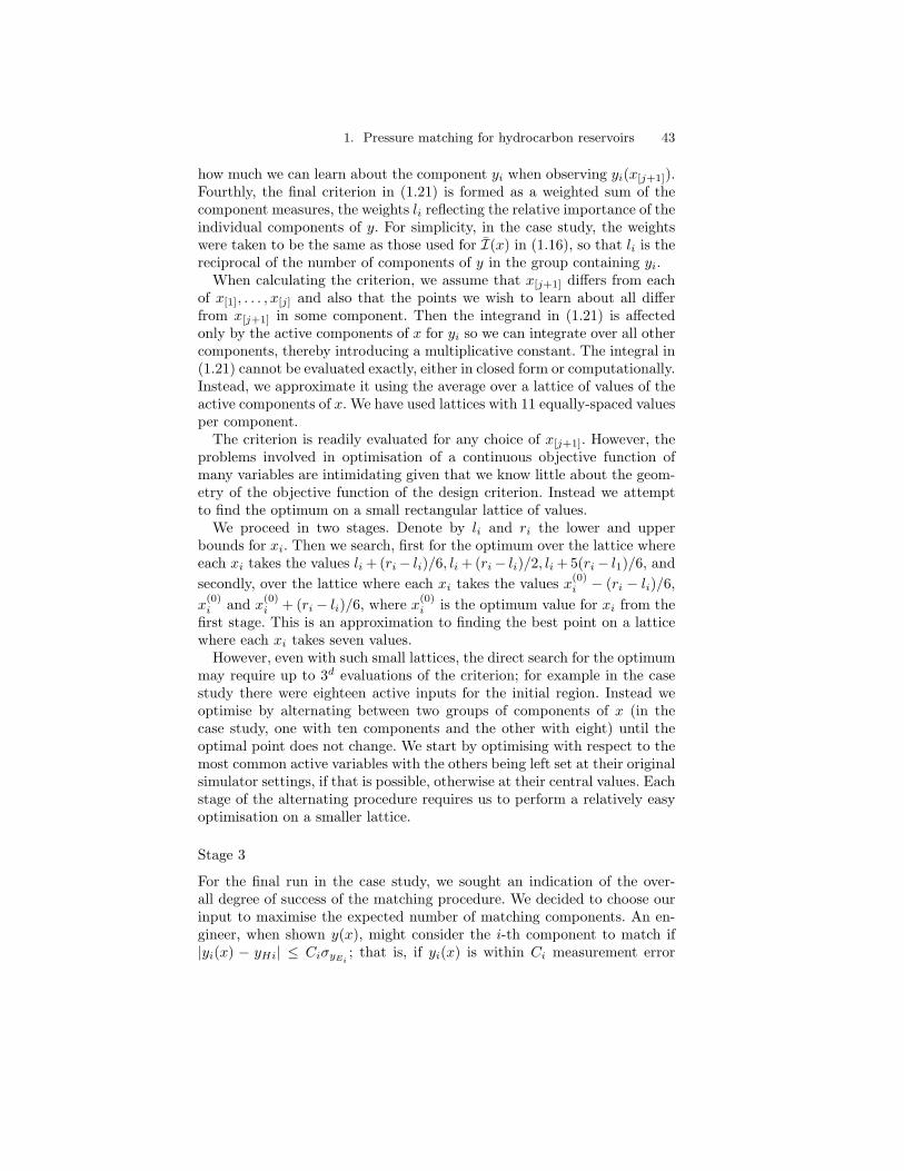
1. Pressure matching for hydrocarbon reservoirs 43
how much we can learn about the component yi when observing yi(x[j+1]).Fourthly, the final criterion in (1.21) is formed as a weighted sum of thecomponent measures, the weights li reflecting the relative importance of theindividual components of y. For simplicity, in the case study, the weightswere taken to be the same as those used for I(x) in (1.16), so that li is thereciprocal of the number of components of y in the group containing yi.
When calculating the criterion, we assume that x[j+1] differs from eachof x[1], . . . , x[j] and also that the points we wish to learn about all differfrom x[j+1] in some component. Then the integrand in (1.21) is affectedonly by the active components of x for yi so we can integrate over all othercomponents, thereby introducing a multiplicative constant. The integral in(1.21) cannot be evaluated exactly, either in closed form or computationally.Instead, we approximate it using the average over a lattice of values of theactive components of x. We have used lattices with 11 equally-spaced valuesper component.
The criterion is readily evaluated for any choice of x[j+1]. However, theproblems involved in optimisation of a continuous objective function ofmany variables are intimidating given that we know little about the geom-etry of the objective function of the design criterion. Instead we attemptto find the optimum on a small rectangular lattice of values.
We proceed in two stages. Denote by li and ri the lower and upperbounds for xi. Then we search, first for the optimum over the lattice whereeach xi takes the values li + (ri− li)/6, li + (ri− li)/2, li + 5(ri− l1)/6, andsecondly, over the lattice where each xi takes the values x(0)
i − (ri − li)/6,x
(0)i and x(0)
i + (ri − li)/6, where x(0)i is the optimum value for xi from the
first stage. This is an approximation to finding the best point on a latticewhere each xi takes seven values.
However, even with such small lattices, the direct search for the optimummay require up to 3d evaluations of the criterion; for example in the casestudy there were eighteen active inputs for the initial region. Instead weoptimise by alternating between two groups of components of x (in thecase study, one with ten components and the other with eight) until theoptimal point does not change. We start by optimising with respect to themost common active variables with the others being left set at their originalsimulator settings, if that is possible, otherwise at their central values. Eachstage of the alternating procedure requires us to perform a relatively easyoptimisation on a smaller lattice.
Stage 3
For the final run in the case study, we sought an indication of the over-all degree of success of the matching procedure. We decided to choose ourinput to maximise the expected number of matching components. An en-gineer, when shown y(x), might consider the i-th component to match if|yi(x) − yHi| ≤ CiσyEi ; that is, if yi(x) is within Ci measurement error
44 Peter S. Craig, Michael Goldstein, Allan H. Seheult, James A. Smith
standard deviations of the corresponding historical value. The choice of Cimight be made according to an engineering criterion of match quality orsome standard value might be used. As an approximation, we calculate theprobability of this event assuming that yi(x) has some convenient distribu-tion parametrised by its mean and standard deviation. The sum of theseprobabilities is the expected number of matching components of y.
We can project this expectation into a smaller number of componentsof x in the same way as we did for implausibility but this time taking themaximum over the components being eliminated. To choose the point toevaluate, we find the value of x which has the highest expected numberof matching components. This calculation can be done by back-trackingthrough the projection process having projected onto a couple of variablesand having found the best value for those variables. All that is requiredis to store the grids formed by combining variables at each stage of theprojection.
11 Case Study: Further Details
We have described how our prior descriptions were formed, how they wereused to select runs on the simulator, how we used plausibility maps torestrict the original region to a smaller sub-region, and how diagnosticscaused us to change our prior description. We now give further details ofthe application of the methodology to the sub-region where x3 ≥ −0.6,x4 ≤ −0.2 and where all other components of x vary over the originalrange of [−1, 1].
We ran a fast simulator hypercube of size 100 on the sub-region andbuilt descriptions using the process outlined in Section 7.2. In stage 2 ofthis process, we took the two previous runs which fell in our sub-region asavailable data, and in stage 3 took the standard deviation of the differencein coefficient values for the simulators to be 20% of the magnitude of thecoefficient estimate from the fast simulator data instead of the original 5%.
Data analysis of the least squares fits suggested a square root transfor-mation for x components representing transmissibilities of faults, as thisresults in a better quadratic fit. Descriptions were then rebuilt using thesame fast simulator data. It should be noted that, as a result, the hypercubeis no longer orthogonal in the new coordinate system.
The collections of active variables chosen for components for the sub-region differed substantially from those for the original region, but in amanner consistent with the change of region. For many components, x3 orx4 was replaced by a permeability multiplier for a nearby region or a trans-missibility multiplier for a nearby fault. Where the same active variableswere chosen, their order of importance often changed. Means of coefficientsfor terms also changed substantially, but usually without changing sign.
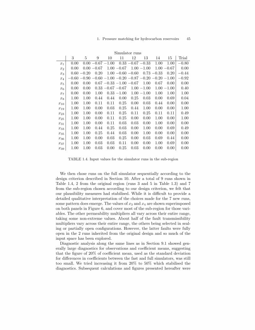
1. Pressure matching for hydrocarbon reservoirs 45
Simulator runs3 5 9 10 11 12 13 14 15 Trial
x1 0.00 0.00 −0.67 −1.00 0.33 −0.67 −0.33 1.00 1.00 −0.80x2 0.00 0.00 −0.67 1.00 −0.67 1.00 −1.00 1.00 −0.67 0.00x3 0.60 −0.20 0.20 1.00 −0.60 −0.60 0.73 −0.33 0.20 −0.44x4 −0.60 −0.90 −0.60 −1.00 −0.20 −0.87 −0.20 −0.20 −1.00 −0.92x5 0.00 0.00 0.67 −0.33 −1.00 −0.67 1.00 0.67 0.00 0.00x6 0.00 0.00 0.33 −0.67 −0.67 1.00 −1.00 1.00 −1.00 0.40x7 0.00 0.00 1.00 0.33 −1.00 1.00 −1.00 1.00 1.00 1.00x8 1.00 1.00 0.44 0.44 0.00 0.25 0.03 0.00 0.69 0.04x10 1.00 1.00 0.11 0.11 0.25 0.00 0.03 0.44 0.00 0.00x19 1.00 1.00 0.00 0.03 0.25 0.44 1.00 0.00 0.00 1.00x23 1.00 1.00 0.00 0.11 0.25 0.11 0.25 0.11 0.11 0.49x25 1.00 1.00 0.00 0.11 0.25 0.00 0.00 1.00 0.00 1.00x31 1.00 1.00 0.00 0.11 0.03 0.03 0.00 1.00 0.00 0.00x33 1.00 1.00 0.44 0.25 0.03 0.00 1.00 0.00 0.69 0.49x35 1.00 1.00 0.25 0.44 0.03 0.00 1.00 0.00 0.00 0.00x36 1.00 1.00 0.00 0.03 0.25 0.00 0.03 0.69 0.44 0.00x37 1.00 1.00 0.03 0.03 0.11 0.00 0.00 1.00 0.69 0.00x39 1.00 1.00 0.03 0.00 0.25 0.03 0.00 0.00 0.00 0.00
TABLE 1.4. Input values for the simulator runs in the sub-region
We then chose runs on the full simulator sequentially according to thedesign criterion described in Section 10. After a total of 9 runs shown inTable 1.4, 2 from the original region (runs 3 and 5 in Table 1.3) and 7from the sub-region chosen according to our design criterion, we felt thatour plausibility measures had stabilised. While it is difficult to provide adetailed qualitative interpretation of the choices made for the 7 new runs,some pattern does emerge. The values of x3 and x4 are shown superimposedon both panels in Figure 6, and cover most of the sub-region for those vari-ables. The other permeability multipliers all vary across their entire range,taking some non-extreme values. About half of the fault transmissibilitymultipliers vary across their entire range, the others being selected in seal-ing or partially open configurations. However, the latter faults were fullyopen in the 2 runs inherited from the original design and so much of theinput space has been explored.
Diagnostic analysis along the same lines as in Section 9.1 showed gen-erally large diagnostics for observations and coefficient means, suggestingthat the figure of 20% of coefficient mean, used as the standard deviationfor differences in coefficients between the fast and full simulators, was stilltoo small. We tried increasing it from 20% to 50% which stabilised thediagnostics. Subsequent calculations and figures presented hereafter were
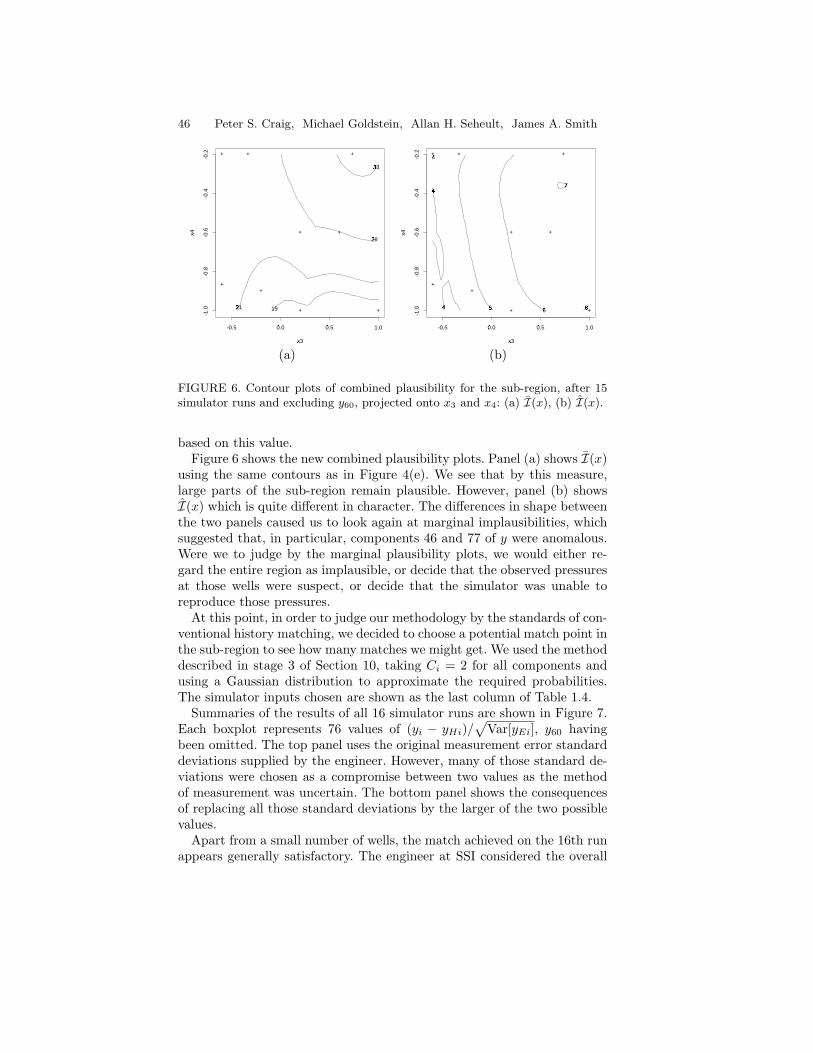
46 Peter S. Craig, Michael Goldstein, Allan H. Seheult, James A. Smith
x3�
x4
-0.5 0.0�
0.5�
1.0
-1.0
-0.8
-0.6
-0.4
-0.2
1921�
26�
33�
+
+
+
+
+
+
++
+
x3�
x4
-0.5 0.0�
0.5�
1.0
-1.0
-0.8
-0.6
-0.4
-0.2
4�
4�
4�
5�
6� 6
�
7�
+
+
+
+
+
+
++
+
(a) (b)
FIGURE 6. Contour plots of combined plausibility for the sub-region, after 15simulator runs and excluding y60, projected onto x3 and x4: (a) I(x), (b) I(x).
based on this value.Figure 6 shows the new combined plausibility plots. Panel (a) shows I(x)
using the same contours as in Figure 4(e). We see that by this measure,large parts of the sub-region remain plausible. However, panel (b) showsI(x) which is quite different in character. The differences in shape betweenthe two panels caused us to look again at marginal implausibilities, whichsuggested that, in particular, components 46 and 77 of y were anomalous.Were we to judge by the marginal plausibility plots, we would either re-gard the entire region as implausible, or decide that the observed pressuresat those wells were suspect, or decide that the simulator was unable toreproduce those pressures.
At this point, in order to judge our methodology by the standards of con-ventional history matching, we decided to choose a potential match point inthe sub-region to see how many matches we might get. We used the methoddescribed in stage 3 of Section 10, taking Ci = 2 for all components andusing a Gaussian distribution to approximate the required probabilities.The simulator inputs chosen are shown as the last column of Table 1.4.
Summaries of the results of all 16 simulator runs are shown in Figure 7.Each boxplot represents 76 values of (yi − yHi)/
√Var[yEi], y60 having
been omitted. The top panel uses the original measurement error standarddeviations supplied by the engineer. However, many of those standard de-viations were chosen as a compromise between two values as the methodof measurement was uncertain. The bottom panel shows the consequencesof replacing all those standard deviations by the larger of the two possiblevalues.
Apart from a small number of wells, the match achieved on the 16th runappears generally satisfactory. The engineer at SSI considered the overall
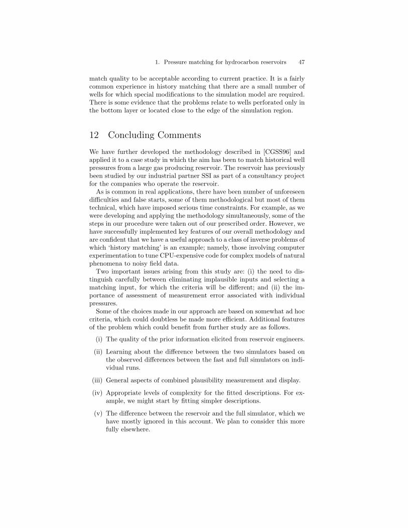
1. Pressure matching for hydrocarbon reservoirs 47
match quality to be acceptable according to current practice. It is a fairlycommon experience in history matching that there are a small number ofwells for which special modifications to the simulation model are required.There is some evidence that the problems relate to wells perforated only inthe bottom layer or located close to the edge of the simulation region.
12 Concluding Comments
We have further developed the methodology described in [CGSS96] andapplied it to a case study in which the aim has been to match historical wellpressures from a large gas producing reservoir. The reservoir has previouslybeen studied by our industrial partner SSI as part of a consultancy projectfor the companies who operate the reservoir.
As is common in real applications, there have been number of unforeseendifficulties and false starts, some of them methodological but most of themtechnical, which have imposed serious time constraints. For example, as wewere developing and applying the methodology simultaneously, some of thesteps in our procedure were taken out of our prescribed order. However, wehave successfully implemented key features of our overall methodology andare confident that we have a useful approach to a class of inverse problems ofwhich ‘history matching’ is an example; namely, those involving computerexperimentation to tune CPU-expensive code for complex models of naturalphenomena to noisy field data.
Two important issues arising from this study are: (i) the need to dis-tinguish carefully between eliminating implausible inputs and selecting amatching input, for which the criteria will be different; and (ii) the im-portance of assessment of measurement error associated with individualpressures.
Some of the choices made in our approach are based on somewhat ad hoccriteria, which could doubtless be made more efficient. Additional featuresof the problem which could benefit from further study are as follows.
(i) The quality of the prior information elicited from reservoir engineers.
(ii) Learning about the difference between the two simulators based onthe observed differences between the fast and full simulators on indi-vidual runs.
(iii) General aspects of combined plausibility measurement and display.
(iv) Appropriate levels of complexity for the fitted descriptions. For ex-ample, we might start by fitting simpler descriptions.
(v) The difference between the reservoir and the full simulator, which wehave mostly ignored in this account. We plan to consider this morefully elsewhere.

48 Peter S. Craig, Michael Goldstein, Allan H. Seheult, James A. Smith
(vi) Match quality. For example, we might monitor variables which arenot formally included in the matching process or examine trends.
(vii) Use of detailed prior information about reservoir properties.
(viii) More decision theoretic views as to how many runs we should take,balancing costs and benefits of continuing or stopping by quantifyingthe value of the match for prediction using the simulator and forlearning about the reservoir.
(ix) The integration of the various stages of our methodology into a singletool. This would seem desirable if the approach is to be used fordecision support.
(x) The advantages and disadvantages of using joint versus marginal co-variance structures. In particular, it would be useful to develop a co-herent covariance structure for the different pressures that properlyreflects their spatial and temporal features.
(xi) The dramatic variation in simulator run time for different inputs. Ourdecision choices should reflect this variation.
Acknowledgements
We are especially grateful to Adam Little and Bob Parish at ScientificSoftware-Intercomp (UK), our industrial collaborators, for their supportand for making available the case study and reservoir simulator. This workhas been supported by a United Kingdom Engineering and Physical Sci-ences Research Council grant under their Complex Stochastic Systems Ini-tiative. We would like to thank the referees and editor for their carefulreading of the paper.
13 References
[CGSS96] P.S. Craig, M. Goldstein, A.H. Seheult, and J.A. Smith. Bayeslinear strategies for matching hydrocarbon reservoir history.In Berger et al., editors, Bayesian Statistics 5. Oxford, 1996.
[FG93] M. Farrow and M. Goldstein. Bayes linear methods forgrouped multivariate repeated measurement studies with ap-plication to crossover trials. Biometrika, 80:39–59, 1993.
[Gol96] M. Goldstein. Prior inferences for posterior judgements. InM. L. D. Chiara et al., editors, 10th International Congressof Logic, Methodology and Philosophy of Science. Kluwer, toappear, 1996.

1. Pressure matching for hydrocarbon reservoirs 49
[Inc93] Statistical Sciences Inc. S-PLUS Reference Manual, Version3.2. StatSci, a division of MathSoft Inc., Seattle, 1993.
[MCB79] M.D. McKay, W.J. Conover, and R.J. Beckham. A compar-ison of three methods for selecting values of input variablesin the analysis of output of computer code. Technometrics,21:239–245, 1979.
[MD90] C. C. Mattax and R. L. Dalton. Reservoir Simulation. Societyof Petroleum Engineers, 1990.
[Puk94] F. Pukelsheim. The three sigma rule. The American Statisti-cian, 48:88–91, 1994.
[SWMW89] J. Sacks, W. Welch, T. Mitchell, and H. Wynn. Design andanalysis of computer experiments. Statistical Science, 4:409–435, 1989.
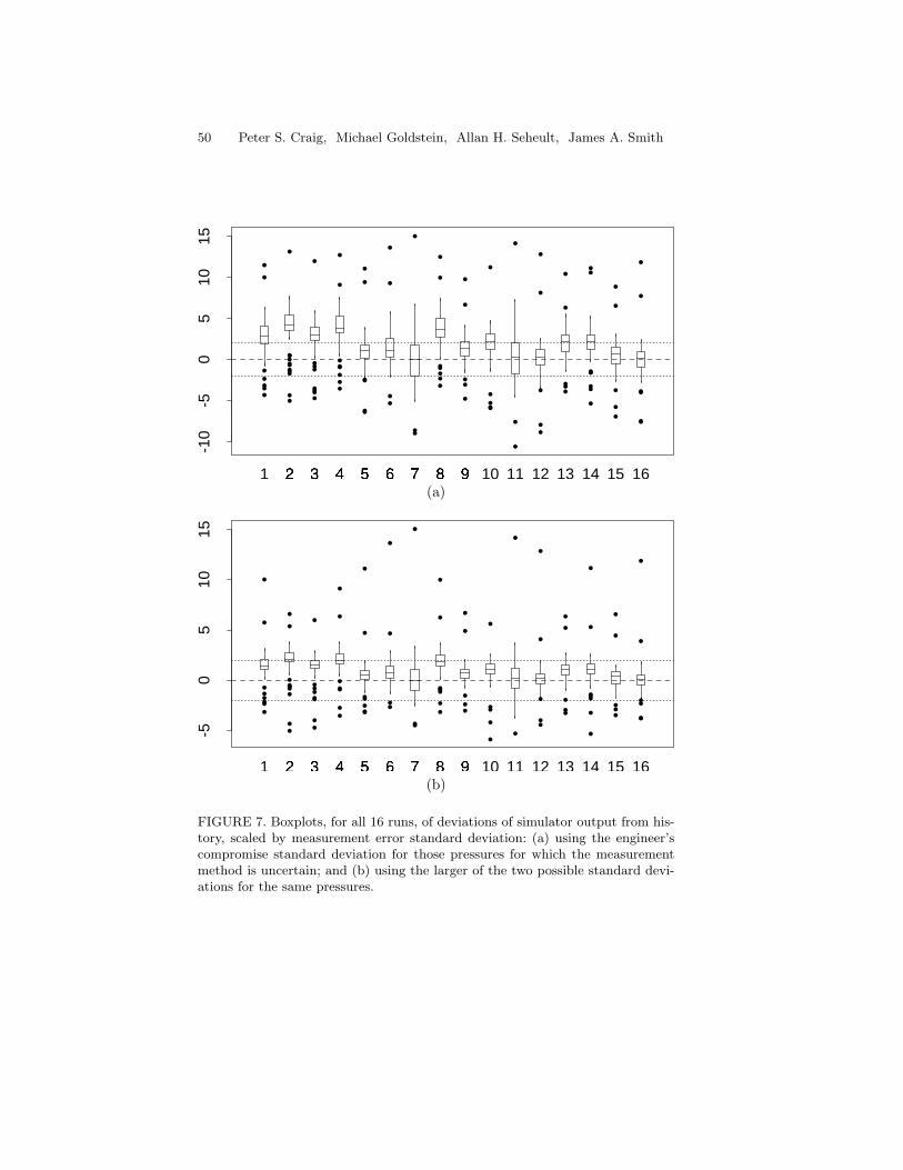
50 Peter S. Craig, Michael Goldstein, Allan H. Seheult, James A. Smith
-10
-50
510
15
•••••
••
••••••••••
•
•••••••
•
••••••
•
•
••
••
••
••
•
•
••
•
•••••
••
•••
•
•
••••
•
•
•
•
••
•
•
•
•••
•
•
••••••
••
•••
••
••
••
•
•
1 2�
3�
4�
5�
6�
7�
8�
9�
10 11 12 13 14 15 16(a)
-50
510
15
••••••
•
•
••
••••••
••
•••••••
•
•••••
•
•
•••••
•
•
••
•
•
••
•
••••••
•
•
•••
••
••••
•
•
•
•••
•
•
•••
••
•••••
•
•
•••
••
••••
•
•
1 2�
3�
4�
5�
6�
7�
8�
9�
10 11 12 13 14 15 16(b)
FIGURE 7. Boxplots, for all 16 runs, of deviations of simulator output from his-tory, scaled by measurement error standard deviation: (a) using the engineer’scompromise standard deviation for those pressures for which the measurementmethod is uncertain; and (b) using the larger of the two possible standard devi-ations for the same pressures.