Embed Size (px)
DESCRIPTION
An overview of turbocharger history with a focus on turbocharger matching via the Winkler Turbocharger matching method, where the necessary equations are derived from first principles.A turbocharger matching project is undertaken as well as providing full MATLAB simulation source-code.
Citation preview

CONSTANT-PRESSURE TURBOCHARGER MATCHING
9th December 2009
Michael de Silva

i
TABLE OF CONTENTS
1 INTRODUCTION ................................................................................................ 12 TURBOCHARGING............................................................................................ 22.1 TurbochargerComponents...............................................................................................................72.2 AvailableTechnology..........................................................................................................................82.2.1 VariableGeometryTurbocharger(VGT) ..............................................................................................82.2.2 Turbine‐sideBypass(Wastegate)......................................................................................................... 102.2.3 TwinEntryTurbine..................................................................................................................................... 102.2.4 Water‐CooledTurbineHousing............................................................................................................. 11
3 TURBOCHARGERMATCHING .......................................................................... 113.1 WinklerTurbochargerMatchingMethod .................................................................................123.1.1 FirstQuadrant ............................................................................................................................................... 153.1.2 SecondQuadrant .......................................................................................................................................... 173.1.3 ThirdQuadrant ............................................................................................................................................. 183.1.4 FourthQuadrant........................................................................................................................................... 19
4 TURBOCHARGERMATCHINGPROJECT............................................................ 214.1 Task1 ....................................................................................................................................................214.2 Task2 ....................................................................................................................................................235 APPENDIXA:MATLABSIMULATIONCODE...................................................... 27

1
1 INTRODUCTION
Dr. Nickolaus A. Otto invented the four-stroke engine in 1876; twenty years later,
Rudolf Diesel created the very first supercharger design. Sir. Dugald Clark
discovered in 1901 that an engine was capable of producing more power if the
volume of air entering the cylinders was artificially increased (Allard, 1986).
It was only in 1902 that Frenchman Louis Renault patented a system that utilised a
centrifugal fan to drive air into the carburettor via its inlet. Five years late, American
Lee Chadwick and J. T. Nicholls implemented a centrifugal compressor to place the
carburettor under pressure thereby increasing its volumetric efficiency, whereas the
first successful modern turbocharger to be driven by the exhaust gasses of the engine
was developed in 1905 by Swiss Dr. Alfred J. Buchi (Humphries, 1992).
The First World War greatly advanced supercharger technology, as this enabled
fighter aircraft and bombers to reach much higher altitudes. Naval vessels also
greatly benefitted from turbocharged diesel engines; in 1925, one of the first
successful applications of a turbocharged diesel engine was in a German ship capable
of 2000 hp (Amann, 1992).
Turbochargers were once again in demand in World War II, where they proved
successful in aircraft such as the B-17 Flying Fortress, P-47 Thunderbolt, and P-38
Lightning (Logan and Roy, 2003). Between 1950 and the Second World War,
turbochargers were commonly found fitted to diesel truck engines in a commercial
capacity. Due to the much higher power densities and improved fuel consumption the
application of turbocharging large diesel truck engines, typically with a displacement
size exceeding 6 litres in capacity, is the industry standard in their production.

2
2 TURBO CHARGING
Supercharging an engine is the process by which a mechanically driven “air pump”,
or compressor, is utilised to artificially provide a much larger amount of fuel-air
mixture to the engine cylinders than normally taken in by naturally aspirated (non-
supercharged) engines.
The basic concept of most of the supercharging devices available is an increase in
pressure of the fuel-air mixture delivered to the cylinders results in an increase in the
density and the mass flow rate of air drawn into the cylinders during each intake
stroke (Mezger, 1978). It is therefore possible to burn more fuel during a combustion
cycle, if the same ratio of air-to-fuel is maintained, and thereby generate more power.
Therefore, a supercharged engine is able to significantly generate more power and
torque than a naturally aspirated, yet identical engine in terms of displacement size.
Conversely, a lighter supercharged engine with a smaller displacement size is capable
of producing the same power and torque as a heavier and larger normally aspirated
engine.
Figure 1: Supercharged engine; the compressor is driven
off the crankshaft (BorgWarner Turbo Systems, 2009)
Figure 2: Turbocharged engine; the compressor is driven
by a gas turbine running off the engine’s exhaust gasses
(BorgWarner Turbo Systems, 2009)
When the source of mechanical power is obtained directly from the engine crankshaft,
the system is classified as a supercharger, where a compressor is directly driven off
the crankshaft. A turbocharger (turbo supercharger) has its centrifugal compressor

3
driven by the engines exhaust gasses; the compressor is axially connected to a
centripetal radial-inflow exhaust-gas turbine via a common shaft. The turbocharger
system is ineffective at low engine speeds due to the introduction of an exhaust
backpressure, and as such the energy of the exhaust gasses are insufficient to
efficiently operate the turbocharger (Schorr, 1979). Therefore, superchargers are
more suited for operation at low engine speeds.
Turbochargers offer two main advantages; the power density of the engine is
increased, and particularly in diesel engines, the specific fuel consumption may be
improved. Exhaust emission due to turbocharging is not adversely effected, as studies
have previously shown, and claims have been made to suggest that typical fuel
consumption is reduced by 20-25% (Schruf and Mayer, 1981). Of course, the
operational characteristics of a turbocharged engine greatly depend on its application.
The characteristics include maximum power output to high torque over a wide engine
RPM (Revolutions Per Minute) while maintaining low fuel consumption.
Turbocharged engines are greatly preferred in industrial and military applications due
to their high power densities.
Figure 3: Turbocharger arrangement, with the compressor and turbine sections (Zinner, 1978)
A logical overview of the mechanical arrangement of a Turbocharger is shown above
in Figure 3, as well as both the compressor and turbine sections. As seen in the

4
illustration above, the hot exhaust gases drive the turbine that is connected to a shaft,
common to both the turbine and compressor, and is held in place by a bearing system.
Figure 4: Diesel engine Turbocharger (BorgWarner Turbo Systems, 2009)
The bearing system not only provides the required lubrication for the continued
operation of the shaft but it also serves to isolate both the chambers from each other.
Since the power generated by the gas turbine drives the compressor impeller, they
both rotate as the same radial velocity, and the air drawn in from the ambient air inlet
is compressed for delivery to the cylinders. The control system, as shown in Figure 4,
serves to alter the operational parameters of the Turbocharger based on the engines
performance (MacInnes, 1984).
The centrifugal forces exerted by the compressor impeller accelerate the air to
extremely high velocities thereby reaching a high level of kinetic energy. This
kinetic energy is transformed into an increase in static pressure, in the diffuser section
where its cross-sectional area increases gradually. With the rise in air pressure, the
velocity of the air decreases and the air flowing along the perimeter of the diffuser is
collected by a volute and delivered to the air outlet and flows to the cylinders of the
engine. The process by which the high velocity, low pressure air is converted into a
low velocity, high-pressure stream is called diffusion. The ambient air is drawn into
the compressor at the ambient temperature of the immediate surroundings, and at a
similar atmospheric pressure. Once compressed, this air is delivered to the air outlet
at temperatures nearing 200°C.
While the compression of the air drawn in by the compressor increases the boost
pressure and charge density, it results in an increase in the temperature of the air as
well. As described by Charles’ Law, an increase in the volume of the air takes place

5
and therefore slightly reduces the charge density. A more immediate concern due to
the increase in temperature is the excessive thermal stresses placed on the engine and
its operating parts, which could ultimately results in pre-ignition or detonation. Figure 3,
illustrates the implementation of an intercooler (or aftercooler) between the
compressor and cylinder intake; this cooling is achieved either with air or water. The
reduction in air temperature not only improves the volumetric efficiency, due to the
density of the air increasing as a result of drop in volume – as determined by Charles’
Law, but also ensures the increase in compression ratio without the overheating of the
cylinder heads. The higher compression offers for improved low RPM output (Stone,
1999).
Turbochargers were typically limited to diesel engines due to the high operational
temperatures of petrol engine exhaust gases far exceeding the operational capabilities
of the materials typically used in the construction of Turbochargers. However,
advances in materials derived from aerospace technology has resulted in the
development of the first Turbocharged petrol engine, developed by BorgWarner
Turbo Systems (2009), and is currently featured in the Type 997 Porsche 911 Turbo
(Paultan.org, 2009).
One of the disadvantages of turbocharging has been commonly termed “Turbo lag” or
“Turbocharger lag”. Since the exhaust gases drive the turbine, Turbo lag is the delay
experienced during the time taken for the turbine to ‘spool’ up and match the exhaust
air velocity. During this period, less power output is experienced until the turbine
spools up to reach the necessary radial velocity to supply optimal boost pressure. As
the demand of torque fluctuates based on the need to accelerate and decelerate the
turbine rotor, to and from high radial velocities, the resulting delay may take several
seconds due to the rotational inertia of the turbine rotor affecting its response to
changes in the exhaust air flow.
Another phenomenon affecting turbochargers is commonly known as the “Surge
effect”. The surge limit is shown in plots of typical turbocharger compressor maps,
Figure 5 and Figure 6. If the compression energy given to the gas by the compressor falls
below that needed to prevail over the adverse pressure gradient between the ambient
air inlet and compressor outlet, the flow of air suddenly collapses. The sudden

6
collapse in airflow results in the output pressure of the compressor dropping to a
sufficient level, thereby re-establishing in the flow of air and this process continues to
repeat in a cyclic manner. Both the turbocharger compressor maps in Figure 5 and Figure 6
show the surge limit and compressor efficiency in terms of the pressure ratio and rate
of non-dimensional mass flow.
Figure 5: Typical Turbocharger compressor map (Logan
and Roy, 2003)
Figure 6: “Typical performance map (pressure ratio plotted
against mass flow parameter, where N is the rotational
speed of the rotor and T and P the absolute temperature and
pressure) for a compressor without a vaned diffuser. The
surge limit is shown clearly on the left, and the limit on the
right is that set by choking of the flow. Between the two are
the loops of constant efficiency. The horizontal arcs
represent constant-speed conditions” (Garrett, Newton and
Steeds, 2000)
Turbocharging is achieved one of two ways: constant pressure and pulse
turbocharging. In constant pressure turbocharging, the exhaust gas is essentially
discharged into a large manifold (plenum) so as to reduce the magnitude of its
pulsations before entering the turbine. While energy conversion efficiency within the
turbine is greater than in pulse turbocharging, much of the kinetic energy of the gas is
lost on leaving the exhaust ports. This is due to the exhaust gas, initially travelling at
a near sonic velocity, ultimately mixing turbulently with the relatively larger volume
of gas in the large manifold as it discharges. Further more, potentially significant heat
loses from the exhaust gas may occur if the plenum is not thermally insulated.
7
The primary disadvantage of pulse turbocharging is its inherently lower efficiency in
energy conversion in comparison with constant pressure turbocharging. Appropriate
manifold design will compensate for this disadvantage, and account for the decrease
in turbine efficiency due to pulsation of the turbine flow. In modern automotive
applications pulse turbocharging is the de facto standard, whereas constant pressure
turbocharging is implemented in engines with a relatively large displacement size and
is therefore typically utilised in large industrial engines.
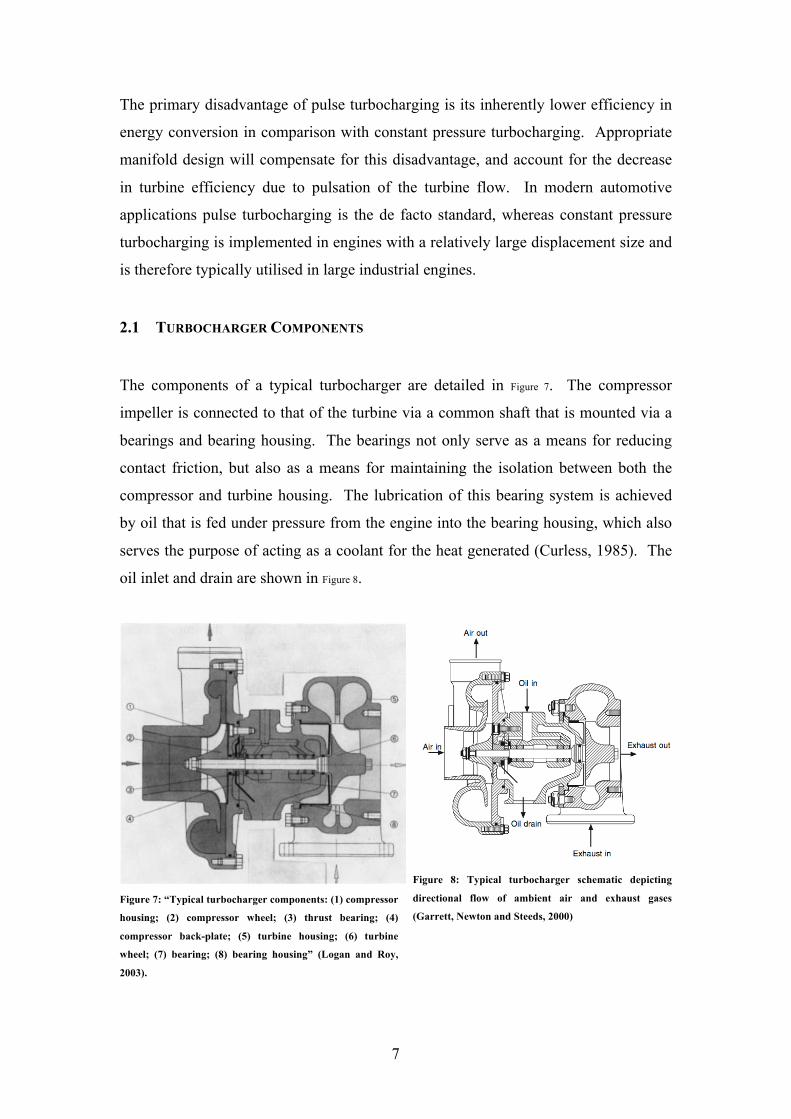
2.1 TURBOCHARGER COMPONENTS
The components of a typical turbocharger are detailed in Figure 7. The compressor
impeller is connected to that of the turbine via a common shaft that is mounted via a
bearings and bearing housing. The bearings not only serve as a means for reducing
contact friction, but also as a means for maintaining the isolation between both the
compressor and turbine housing. The lubrication of this bearing system is achieved
by oil that is fed under pressure from the engine into the bearing housing, which also
serves the purpose of acting as a coolant for the heat generated (Curless, 1985). The
oil inlet and drain are shown in Figure 8.
Figure 7: “Typical turbocharger components: (1) compressor
housing; (2) compressor wheel; (3) thrust bearing; (4)
compressor back-plate; (5) turbine housing; (6) turbine
wheel; (7) bearing; (8) bearing housing” (Logan and Roy,
2003).
Figure 8: Typical turbocharger schematic depicting
directional flow of ambient air and exhaust gases
(Garrett, Newton and Steeds, 2000)

8
The turbine driven by the exhaust gases consists of both the turbine wheel and the
turbine housing, where the energy of the exhaust gases enables the rotation of the
turbine. Once the exhaust gases pass through the blades of the turbine, they are
discharged from the turbine housing through the exhaust outlet, shown in Figure 8.
As the velocity of the exhaust gases is proportional to the speed of the engine, the
rotational velocity of the turbine wheel is thus proportional to the operational speed of
the engine. Turbines are therefore ineffective at lower engine RPMs as the exhaust
gas energy needs to overcome the inertia of the turbine rotor, to set it in motion, and
thereby provide boost pressure; at low RPMs, turbocharged engines therefore tend to
behave like that of a naturally aspirated equivalent.
Similarly, the compressor consists of the compressor wheel (impeller) and compressor
housing. The compressor impeller therefore rotates at same rotational velocity as that
achieved by the turbine wheel and compresses the ambient air drawn in from the air
inlet.
2.2 AVAILABLE TECHNOLOGY
As turbocharges are implemented in a wide variety of applications, the requirements
of these turbocharging systems vary greatly. The following techniques and solutions
are utilised in turbocharged engines so as to obtain the optimum output, depending on
the application of choice. Typical solutions vary in terms of geometrical alterations,
to additional compensatory mechanisms. A few of these techniques are presented in
the following section.
2.2.1 Variable Geometry Turbocharger (VGT)
A Variable Turbine Geometry turbocharger is commonly known as a Variable
Geometry Turbocharger (VGT) as well as a Variable Nozzle Turbine (VNT). These
are a group of turbochargers designed to allow for the effective aspect ratio
(commonly called A/R ratio) to be altered depending on operational conditions.

9
The optimum aspect ratio of a Turbocharged engine at low engine RPMs is
significantly different to that of an engine operating at much higher RPMs. Too large
an aspect ratio will result in the engine being unable to generate sufficient boost
pressure at low RPMs. Conversely, too small an aspect ratio will result in the choking
of the engine and ultimately leading to lower power output (Hishikawa, Okazaki and
Busch, 1988).
Figure 9: Porsche VGT with the turbine guide vanes
“semi-closed” (Paultan.org, 2009).
Figure 10: Exhaust flow through the VGT with the turbine
guide vanes “semi-closed” (Paultan.org, 2009).
Figure 11: Porsche VGT with the turbine guide vanes
“open” (Paultan.org, 2009).
Figure 12: Exhaust flow through the VGT with the turbine
guide vanes “open” (Paultan.org, 2009).
The ability to alter the aspect ratio in Variable Geometry Turbochargers allow them to
maintain the optimum aspect ratio during acceleration of the engine, and are therefore
extremely efficient at higher engine RPMs (Okazaki, Matsuo, Matsudaira and Busch,
1988). As a result, many VGT configurations do not require the implementation of a
wastegate for controlling the turbochargers maximum boost pressure; a higher
turbocharger efficiency is also achieved that than with a wastegate.

10
2.2.2 Turbine-side Bypass (Wastegate)
Turbine-side bypass, more commonly called wastegate, is a valve that diverts a
controlled portion of the exhaust gases away from the turbine wheel. The diversion of
the exhaust gasses allows for maintaining the boost pressure of the turbocharger, the
rotational velocity of the turbine is regulated and as such the rotational velocity of the
compressor impeller is controlled (Lundstrom and Gall, 1986). This control is
typically triggered once the boost pressure has reached a particular maximum
threshold, and is achieved by means of a spring-loaded diaphragm specifically
selected to open the exhaust bypass valve once the compressor output pressure
reaches the predetermined maximum threshold. Such an implementation is shown in
Figure 13.
Figure 13: Typical implementation of a turbine wastegate (Garrett, Newton and Steeds, 2000)
2.2.3 Twin Entry Turbine
As pulse turbocharging is the preferred form of
turbocharging, the turbine wheel is subjected to
variable pressure. The pulsation of the entering gases
are optimised in twin entry turbine implementations
as it allows for much higher pressure ratios to develop Figure 14: Twin Entry Turbine
(BorgWarner Turbo Systems, 2009)

11
in a much shorter time, and therefore results in an increase in efficiency.
The chance of interference is greatly reduced during charge exchange cycles as the
engine cylinders are divided into two groups for the exhaust inlets. As a result, a
more efficient mass flow passes through the turbine resulting in a more desirable level
of torque produced in the engine, especially at lower RPMs.
2.2.4 Water-Cooled Turbine Housing
Turbochargers are not limited to automotive
applications, and one of their first uses was in marine
engines. Most marine engine assemblies are greatly
overcrowded and therefore, water-cooled turbine
housing reduces the chance of injuries to maintenance
personnel.
Such installations in relatively large marine engines require a great amount of cooling,
especially those components in direct contact with exhaust gasses; this heated water
may be further used in secondary applications such as cabin heating.
3 TURBOCHARGER MATCHING
The performance of a turbocharger, as illustrated in Figure 6, is dependant upon the
engine speed while being limited by the surge and choke lines. Delivery of the
appropriate amount of air into the engine cylinders requires the matching of the size
of both the compressor and turbine stages to the swept volume, capacity, and the
power rating of the engine (Weaving, 1990)
Matching turbochargers with engines with a limited or constant speed range has
typically proven to be a rather straightforward task.
However, the process or matching turbochargers with automotive engines that are
typically characterised by their greatly varying speeds are accompanied by complex
matching issues.
Figure 15: Water-cooled Turbine
Housing (BorgWarner Turbo
Systems, 2009)

12
The conditions for matching have been derived with the assumption of constant-
pressure turbocharging, and the effect of pulsation is taken into consideration by the
use of a variable. The following four conditions ensure the matching of a
turbocharger with an engine:
• As the compressor and turbine share the same shaft, the compressor shaft
power equals that of the turbine shaft power,
€
PC = PT
• The rate of non-dimensional mass flow through the turbine is related to the
rate of non-dimensional mass flow of air and rate of non-dimensional mass
flow of fuel through the compressor,
€
˙ m T = ˙ m C + ˙ m f = ˙ m C1+λtotast
λtotast
where
€
ast is the stoichiometric air-fuel ratio and
€
λtot is the relative air ratio.
• The operating point must lie on the flow characteristic of the engine at the
given engine speed.
• The rotational velocity of the compressor impeller should be equal to the
rotational velocity of the turbine wheel, as the pressure ratio and rate of air
flow are fixed by the power balance; Both the compressor and turbine
typically share a common shaft, so that,
€
NC = NT
3.1 WINKLER TURBOCHARGER MATCHING METHOD
The Winkler method, developed by Professor Gustav Winkler and detailed in his
1982 paper titled “Matching turbocharger and engine graphically”, is a means to
allow those without access to simulation tools to easily accomplish the task of
turbocharger matching to engines of choice. The greatest success of this process is its
ability to enable engineers, lacking in-depth knowledge in turbocharging and
thermodynamics, to be able to carry out the task of matching successfully – even
without much knowledge of the inner workings of the turbocharger in question. This
is particularly useful during the product development process where alterations in the
13
design continue to take place; the process of re-matching the engine with the altered
operating conditions is made considerably easier by this method.
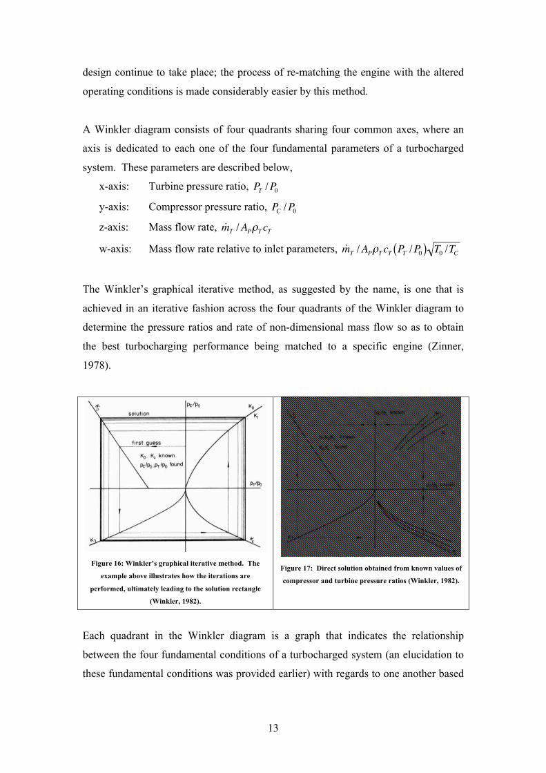
A Winkler diagram consists of four quadrants sharing four common axes, where an
axis is dedicated to each one of the four fundamental parameters of a turbocharged
system. These parameters are described below,
x-axis: Turbine pressure ratio,
€
PT /P0
y-axis: Compressor pressure ratio,
€
PC /P0
z-axis: Mass flow rate,
€
˙ m T / APρT cT
w-axis: Mass flow rate relative to inlet parameters,
€
˙ m T / APρT cT PT / P0( ) T0 /TC
The Winkler’s graphical iterative method, as suggested by the name, is one that is
achieved in an iterative fashion across the four quadrants of the Winkler diagram to
determine the pressure ratios and rate of non-dimensional mass flow so as to obtain
the best turbocharging performance being matched to a specific engine (Zinner,
1978).
Figure 16: Winkler’s graphical iterative method. The
example above illustrates how the iterations are
performed, ultimately leading to the solution rectangle
(Winkler, 1982).
Figure 17: Direct solution obtained from known values of
compressor and turbine pressure ratios (Winkler, 1982).
Each quadrant in the Winkler diagram is a graph that indicates the relationship
between the four fundamental conditions of a turbocharged system (an elucidation to
these fundamental conditions was provided earlier) with regards to one another based
14
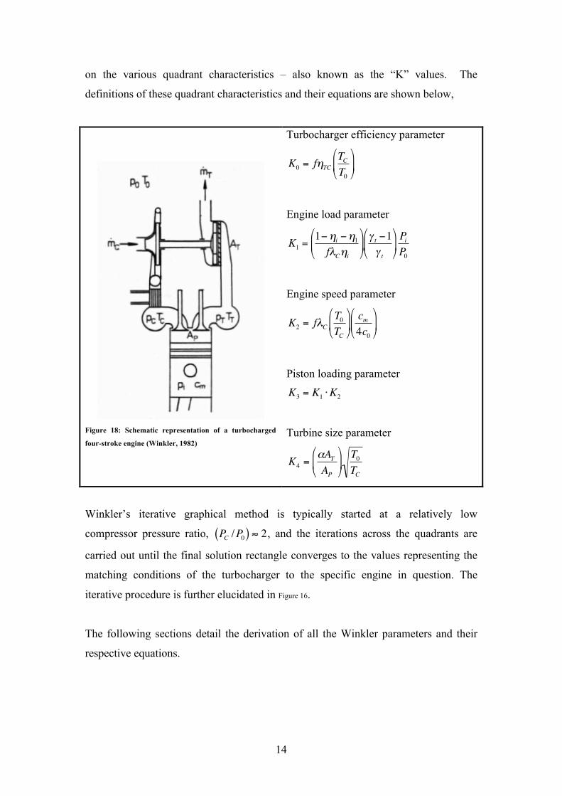
on the various quadrant characteristics – also known as the “K” values. The
definitions of these quadrant characteristics and their equations are shown below,
Figure 18: Schematic representation of a turbocharged
four-stroke engine (Winkler, 1982)
Turbocharger efficiency parameter
€
K0 = fηTCTCT0
Engine load parameter
€
K1 =1−ηi −η1fλCηi
γ t −1γ t
PiP0
Engine speed parameter
€
K2 = fλCT0TC
cm4c0
Piston loading parameter
€
K3 = K1 ⋅K2
Turbine size parameter
€
K4 =αATAP
T0TC
Winkler’s iterative graphical method is typically started at a relatively low
compressor pressure ratio,
€
PC /P0( ) ≈ 2, and the iterations across the quadrants are
carried out until the final solution rectangle converges to the values representing the
matching conditions of the turbocharger to the specific engine in question. The
iterative procedure is further elucidated in Figure 16.
The following sections detail the derivation of all the Winkler parameters and their
respective equations.

15
3.1.1 First Quadrant
A priori knowledge of the exhaust temperature is required to establish the power
equilibrium of the turbocharger. The First Law of Thermodynamics states that energy
is conserved; hence, considering Einstein’s equation of relativity in the form
€
m =Ec2
posits the fact that mass is conserved. Therefore, the fuel energy that is neither
transformed into useful mechanical work nor lost to the environment via cooling may
be found inextricably in the extremely hot exhaust gasses. This can be written as,
€
TT −TC( )mTcp = 1−ηi −η1( )mFCV (1)
The following parameters are introduced,
€
Pi = ηimFCV
VS (2)
€
mT = fλCρCVS (3)
€
ρC =PCRCTC
(4)
Substituting Equation 2 (in terms of
€
mF ) and Equation 3 (in terms of
€
mT ) into
Equation 1, yields the following relationship between the compressor pressure ratio
and temperature ratio,
€
TT −TC( ) fλCρCVScp = 1−ηi −η1( ) PiVSCVηi
CV (5)
Substituting of Equation 4 into Equation 5 and further simplifying,
€
TT −TC( )PCcpRCTC
VS =
1−ηi −η1( )fλCηi
PiVS (6)
Expansion and simplification yields,
€
TTPCcpRCTC
−TCPCcpRCTC
=1−ηi −η1( )fλCηi
Pi (7)

16
€
TTPCTC
− PC =1−ηi −η1( )fλCηi
PiRCcp
(8)
Substituting
€
RCcp
=γ t −1γ t
into Equation 8, above,
€
PCTTTC
−1
=
1−ηi −η1( )fλCηi
Piγ t −1γ t
(9)
€
PCTTTC
=1+
1−ηi −η1( )fλCηi
Piγ t −1γ t
(10)
€
TTTC
=1+1−ηi −η1( )fλCηi
γ t −1γ t
PiP0P0PC
(11)
So as to be able to isolate the engine characteristic parameters in Equation 11, the
characteristic parameter
€
K1 is introduced. As such, Equation 11 simplifies to 13,
€
K1 =1−ηi −η1fλCηi
γ t −1γ t
PiP0
(12)
€
TTTC
=1+K1P0PC
(13)
Winkler (1982) states, “The power equilibrium of the turbocharger is described by
what is sometimes called the first law of turbocharging,” and an expression describing
the relationship between the pressure ratios of the turbine and compressor may be
obtained in consideration of this law,
€
PCP0
= 1+ fηTCcpTcpC
TTT01− P0
PT
γT −1γT
γCγC−1
(14)
Since,
€
TTT0
=TTTC
TCT0
,
€
PCP0
= 1+ fηTCTCT0
cpTcpC
TTTC
1− P0PT
γT −1γT
γCγC−1
(15)

17
€
K0 is introduced, to isolate the engine characteristics,
€
K0 = fηTCTCT0
(16)
€
TTTC
, defined in Equation 13, and
€
K0 are substituted into Equation 15,
€
PCP0
= 1+K0
cpTcpC
1+K1
P0PC
1−
P0PT
γT −1γT
γCγC−1
(17)
3.1.2 Second Quadrant
The characteristic lines in the second quadrant represent a relationship between the
rate of non-dimensional mass flow and the compressor pressure ratio – the air
breathing characteristics of a four-stroke engine (Winkler, 1982). As such, the non-
dimensional mass flow rate is evaluated by the following equation, which relates
turbine mass flow rate to the compressor mass flow rate,
€
˙ m T = f ˙ m C = fλCρCVSn2
(18)
The following parameters are introduced,
€
VS = APS (19)
€
cm = 2Sn (20)
€
ρC =PCRCTC
(21)
The above equations were substituted into Equation 18, yielding,
€
˙ m T = fλCPC
RCTC
APS n2
(22)
€
˙ m TAP
= fλCPC
RCTC
S cm
2S12
= fλCPC
RCTC
cm
4 (23)

18
Substituting
€
RC = R0 into Equation 21 yields
€
R0 =P0T0ρ0
; substituting this into the
previous equation yields,
€
˙ m TAP
= fλCPC
P0
T0ρ0
TC
cm
4= fλC
T0ρ0PC
P0TC
cm
4 (24)
Further simplification is obtained by the introduction of
€
K2 ,
€
K2 = fλCT0TC
cm4c0
(25)
Hence,
€
˙ m TAPρ0c0
= K2PC
P0
(26)
3.1.3 Third Quadrant
Equation 26 is rearranged, as follows, so as to establish a new relationship between
the mass flow rate and the flow conditions before the turbine stage,
€
˙ m TAP
= K2PC
P0
ρ0c0 (27)
The following parameters are introduced,
€
cT = KRTT (28)
€
c0 = KRT0 (29)
€
R =PTρTTT
(30)
Substituting Equation 29 and Equation 30, in terms of
€
ρ0 , into Equation 27 yields,
€
˙ m TAP
= K2PC
P0
P0
RT0
KRT0 (31)

19
Substituting Equation 30 and replacing
€
KRT0 by
€
cT into Equation 31 results in,
€
˙ m TAP
= K2PC
P0
P0
PT
ρTTT
T0
cTT0
TT
= K2PC
P0
ρTTT P0
PTT0
cTT0
TT
(32)
€
˙ m TAPρT cT
= K2PC
P0
P0
PT
TT
T0
T0
TT
(33)
Since
€
x 1x
= x ,
€
˙ m TAPρT cT
= K2PC
P0
P0
PT
TT
T0
T0
= K2PC
P0
P0
PT
TT
T0
(34)
Considering Equation 13 in the form
€
TTTC
= 1+K1P0PC
,
€
˙ m TAPρT cT
= K2PC
P0
1+ K1
P0
PC
P0
PT
TC
T0
(35)
Introducing
€
K3 = K1 ⋅K2 ,
€
˙ m TAPρT cT
PT
P0
T0
TC
= K2
PC
P0
1+
K3
K2PC
P0
(36)
3.1.4 Fourth Quadrant
The characteristic lines in the fourth quadrant relate the rate of non-dimensional mass
flow through the turbine’s exhaust to its pressure ratio. This rate of non-dimensional
mass flow through an equivalent nozzle area is therefore given as,
€
˙ m T = αATρT 2RTTT ψ (37)
where
€
ψ is the turbine flow function parameter for the value of
€
AT and is defined as,
€
ψ =γG
γG −1P4P3
2γG−
P4P3
γG+1γG
(38)

20
Multiplying the left and right hand sides of Equation 37 by
€
1APρTcT
PTP0
T0TC
gives,
€
˙ m TAPρT cT
PT
P0
T0
TC
= αATρT 2RTTT ψ1
APρT cT
PT
P0
T0
TC
(39)
€
K4 is introduced to isolate engine parameters, and is defined as,
€
K4 =αATAP
T0TC
(40)
Introducing
€
cT = γT RTTT and Equation 40 into Equation 39, yields,
€
˙ m TAPρT cT
PT
P0
T0
TC
= K4ψPT
P0
2γT
(41)

21
4 TURBOCHARGER MATCHING PROJECT
4.1 TASK 1
The Ford Puma 2.2L diesel engine is a turbo diesel engine that has a single
turbocharger interfaced with three of its cylinders, hence having a total of two
turbochargers. Winkler’s iterative graphical method is utilised with the assumption of
constant-pressure turbocharging, thereby greatly simplifying the task of matching.
The parameters of each of the Winkler graph quadrants are calculated below as the
first step in the Winkler turbocharger matching process. The operating conditions of
the engine have been supplied in the project specifications.
€
K0 = fηTCTCT0
=1.048× 0.4527×
410.203298
= 0.65306 (42)
€
K1 =1−ηi −η1fλCηi
γ t −1γ t
PiP0
=
1− 0.3821− 0.21321.048 ⋅1.8478 ⋅0.3821
0.351.35
18.81821
(43)
€
K1 =0.40470.739935
0.351.35
18.8182( ) = 2.66841 (44)
€
cm = 2Sn = 2 94.61000
200060
= 6.3067 m/s (45)
€
K2 = fλCT0TC
cm4c0
=1.048 ⋅1.8478
298410.203
6.30674 ⋅ 340
= 6.5237×10⁻³ (46)
€
K3 = K1 ⋅K2 =17.385×10⁻³ (47)
The aspect area of all the pistons is further tripled, as the turbocharger is interfaced
with three cylinders,
€
AP = nπr2( ) = nπ D2
2
n
πD2
4
= 3( ) π (8.6)
2
4
=174.26 cm2 (48)
The flow pulse factor is given as
€
α =1, and therefore,
€
K4 =αATAP
T0TC
=3.7
174.26
298410.203
=18.097×10⁻³ (49)

22
The four quadrants were plotted, utilising the Winkler graph parameters that were
previously calculated, and Winkler’s iterative graphical method was implemented to
determine the pressure ratios of the compressor and turbine as well as their associated
temperature ratio. Once the iterative process was completed, the solution rectangle
was plotted as Figure 19. A developed MATLAB simulation verified the plotted
results yielding an acceptable difference of ~ 2-5% between them (Appendix A).
The following values were obtained from the graph,
€
TTTC
≈ 2.05 (50)
€
PCP0
≈ 2.6 (37.71 PSI of boost pressure) (51)
€
PTP0
≈ 2.55 (52)
Figure 19: Converged solution of the iterative Winkler’s graphical method

23
4.2 TASK 2
This task requires the same turbocharger to be matched to the Ford Puma engine, as in
the previous task, at a decreased engine speed of 1700 rev/min and a compressor
outlet temperature of 320K. As in the previous task, the Winkler graph parameters
are calculated below,
€
K0 = fηTCTCT0
=1.048× 0.4527×
320298
= 0.50945 (53)
€
K1 =1−ηi −η1fλCηi
γ t −1γ t
PiP0
=
1− 0.3821− 0.21321.048 ⋅1.8478 ⋅0.3821
0.351.35
18.81821
(54)
€
K1 =0.40470.739935
0.351.35
18.8182( ) = 2.66841 (55)
€
cm = 2Sn = 2 94.61000
170060
= 5.3607 m/s (56)
€
K2 = fλCT0TC
cm4c0
=1.048 ⋅1.8478
298320
5.36074 ⋅340
= 7.108×10⁻³ (57)
€
K3 = K1 ⋅K2 =18.9678×10⁻³ (58)
The aspect area of all the pistons is further tripled, as the turbocharger is interfaced
with three cylinders,
€
AP = nπr2( ) = nπ D2
2
n
πD2
4
= 3( ) π (8.6)
2
4
=174.26 cm2 (59)
The flow pulse factor is given as
€
α =1 in the specifications, hence,
€
K4 =αATAP
T0TC
=3.7
174.26
298320
= 20.4898×10⁻³ (60)
To ensure the surge effect does not take place the compressor surge line was plotted
in the second quadrant on the Winkler graph, as per the project specifications
indicated values of non-dimensional mass flow rates and pressure ratios of the
compressor surge line.
24
However, the mass flow rate of the compressor specified in the project specifications
needed to be converted from
€
˙ m C into the same form as the z-axis,
€
˙ m TAPρT cT( )
.
The density of air at a temperature of 20°C and pressure of 1 atm or 101.325 kPa,
defined as Normal Temperature and Pressure (NTP), is 1.204 kg/m3. However, at sea
level the density of air is approximately 1.2 kg/m3, and as such
€
ρ0 was taken as 1.2
kg/m3.
Hence, as per Equation 18,
€
f ˙ m CAPρ0c0
=˙ m T
174.2610×10³
1.2( ) 340( )
(61)
Since the calculated value for the aspect area of all the pistons in Equation 56 is in
cm2, care has been taken to convert this to m2 in Equation 58. The values of the
converted form of the non-dimensional mass flow rate of the compressor at their
respective pressure ratios are tabulated in Table 1.
Table 1: Converted values for plotting the compressor surge line in the second
quadrant
€
˙ m TAPρT cT( )
€
PCP0
0.00330 1.317 0.00398 1.5 0.00538 1.717 0.00641 1.983 0.00884 2.317 0.01266 2.733 0.01561 3.25 0.01828 3.75
Due to the avoidance of the “surge effect”, the reduction in the boost pressure of the
turbocharger prevents straightforward matching with the engine at its lower speed. A
solution to this problem is achieved with the implementation of a Variable Geometry
Turbocharger (VGT) and a variable turbine aspect area,
€
AT .

25
Calculating the value for K4 in the fourth quadrant, as performed in Equation 60,
shows
€
AT as an inextricable variable in the formulation. Therefore, the iterative
Winkler graphical method may not be applied in this particular scenario.
It is, however, possible to determine the solution rectangle based on K1, K2, and K3.
Since, it is the value of K4 that determines the curvature of the curve in the fourth
quadrant – multiple plots of varying values for K4 will allow for a manual means for
inspecting the correct curve that intersects the vertex of the solution rectangle in the
fourth quadrant.
Once an appropriate value is obtained for K4, Equation 60 may be re-evaluated to
determine the required turbine aspect area. Utilising the specified value for indicated
mean effective pressure of 18.8182 bars,
€
Pi =qC
λtotastρCεViηi (62)
where the variables above have the following values and definitions,
•
€
qC : the Higher Heating Value (HHV) of diesel, taken as 42.5 MJ/kg
•
€
αst : stoichiometric air-fuel ratio for gasoline, taken as 14.3
•
€
λtot : the fuel equivalence ratio, i.e. the ratio of fuel-air mix to stoichiometric
fuel-air mix, taken as 1.8
•
€
εVi : volumetric efficiency, i.e. how well the cylinder fills, taken as 0.97
Substituting the values above and solving Equation 62 for
€
ρC ,
€
ρC =18.8182×10⁵
42.5×10⁶
1.8×14.3
0.97( ) 0.3821( )
= 3.075 kg/m3 (63)
Substituting the above value for the density, where
€
R = 287 J kg-1 K-1 is the universal
gas constant, and converting from Pascal’s to bars,
€
PC = ρCRTC =3.075( ) 287( ) 320( )100×103
= 2.82 bar or 40.9 PSI boost pressure (64)
€
∴PCP0
= 2.82 (65)

26
The dashed solution rectangle was positioned in Figure 20 with its upper most side
between K1 and K2 with a vertical displacement of
€
PCP0
= 2.82. As such, its vertex in
the fourth quadrant suggests the actual value of K4 is approximately 0.0143. The
following values were obtained from the graph,
€
TTTC
≈ 1.95 (66)
€
PTP0
≈ 4.29 (67)
The effective turbine aspect area from the obtained value for K4 is calculated below,
€
AT =APK4
α
TCT0
=174.26× 0.0143
1
320298
= 2.58226 cm2 (68)
Figure 20: Winkler’s graphical solution based on three fixed positions for K1, K2,
and K3. K4 is required to pass through the solutions vertex in the fourth
quadrant, and is hence determined.

27
5 APPENDIX A: MATLAB SIMULATION CODE
function result = winkler_1
% Engine characteristics and operating parameters
B = 81; % Engine Bore [mm]
S = 94.6; % Engine stroke [mm]
T_0 = 298; % Compressor inlet temperature [K]
P_0 = 1; % Compressor inlet pressure [Bar]
C_0 = 340; % velocity of sound [m/s]
alpha = 1; % Flow pulse factor
f = 1.048; % Mass ration of exhaust gas to air
gamma_t = 1.35; % Gas isentropic exponent
% Specifications for Task 1:
n = 2000; % Engine speed [rev/min]
lambda = 1.8478; % Volumetric efficiency
P_i = 18.8182; % Mean indicated pressure
eta_i = 0.3821; % Indicated efficiency
eta_1 = 0.2132; % Energy loss to coolant relative to fuel energy
T_c = 425; % Compressor temperature [K]
eta_tc = 0.4527; % Turbo charger efficiency
A_t = 3.7; % Effective turbine flow area [cm2]
% Assumption and data collected by author
gamma_c = 1.4; % In the compressor the gas is air
P_t_P_0 = 3; % Turbine pressure ratio
P_c_on_P_0 = 3; % compressor pressure ratio
C_pt = 1107;
C_pc = 1004.5;
% Solution
K_0 = f * eta_tc * (T_c / T_0);
K_1 = ((1 - eta_i - eta_1)/(f * lambda*eta_i)) * ( (gamma_t - 1)/gamma_t ) *
(P_i/P_0);
C_m = 2 * (n * (S/1000))/60;
K_2 = f * lambda * (T_0/T_c) * (C_m / (4 * C_0));
K_3 = K_1 * K_2;
A_p = 3*((pi * (B/10)^2)/4); % The multiplication by 3 is for 3
pistons per stroke
K_4 = (alpha * (A_t/A_p)) * sqrt(T_0/T_c);
% The error variable as an indication of convergence
error = 1;

28
% Calculation of Pc over P0
term_1 = 1;
term_2 = K_0*(C_pt/C_pc);
term_3 = 1 + K_1 * (1/P_c_on_P_0);
term_4 = 1 - (1/P_t_P_0)^( (gamma_t-1)/gamma_t);
P_c_on_P_0 = ( term_1 + term_2 * term_2 * term_3 * term_4) ^ ( gamma_c / (gamma_c
- 1));
while (error > 0.1)
% Calculation of Tt/Tc
T_t_on_T_c = 1+ (K_1 * ( 1 / P_c_on_P_0));
% Calculation of non-dimensionalised mass flow rate
nd_mass = K_2 * P_c_on_P_0;
% Calculation of 3rd quadrant vertical axes
relative_mass_flow = nd_mass * sqrt( 1 + K_3/( nd_mass));
% Calculation for the 4th quadrant
zai = sqrt( ( gamma_t / (gamma_t +1) ) * ( (1/P_t_P_0)^(2/gamma_t) -
(1/P_t_P_0)^((gamma_t + 1)/gamma_t) ));
denominator = K_4* zai * sqrt(2/gamma_t);
P_t_P_0 = relative_mass_flow/denominator;
% All the values at that stage are recorded
answer = [P_c_on_P_0 , P_t_P_0 , nd_mass , relative_mass_flow];
% Calculation of new Pc over P0
term_1 = 1;
term_2 = K_0*(C_pt/C_pc);
term_3 = 1 + K_1 * (1/P_c_on_P_0);
term_4 = 1 - (1/P_t_P_0)^( (gamma_t-1)/gamma_t);
P_c_on_P_0 = ( term_1 + term_2 * term_2 * term_3 * term_4) ^ ( gamma_c / (gamma_c
- 1));
error = abs(answer(1) - P_c_on_P_0);
end
result = answer;

REFERENCES
i Allard, A. (1986) Turbocharging and Supercharging, 2nd edition, Yeovil,
Somerset: Patrick Stephens Ltd.
ii Amann, C.A. (1992) ‘Air-Injection Supercharging—A Page from History’, SAE Paper No. 920843.
iii BorgWarner Turbo Systems (2009) Design and Function of a Turbocharger, http://www.turbodriven.com/en/turbofacts/designTurbine.aspx, Date accessed 8 December 2009.
iv Curless, T. (1985) Turbochargers: Theory, Installation, Maintenance, and Repair,
Osceola: Motorbooks International.
v Garrett, T.K., Newton, K. and Steeds, W. (2000) The Motor Vehicle, 13th edition, Milton Road, Cambridge: Elsevier Science & Technology Books (Butterworth-Heinemann).
vi Hishikawa, A. Okazaki, Y. and Busch, P. (1988) ‘Developments of Variable
Turbine for Small Turbochargers’, SAE Paper No. 880120. vii Humphries, D. (1992) Automotive Supercharging and Turbocharging, Osceola:
Motorbooks International.
viii Logan, E. and Roy, R. (2003) Handbook of Turbomachinery, 2nd edition, Boca Raton, FL: CRC Press.
ix Lundstrom, R.R. and Gall, J.M. (1986) ‘A Comparison of Transient Vehicle
Performance Using a Fixed Geometry, Wastegate Turbocharger and a Variable Geometry Turbocharger’, SAE Paper No. 860104.
x MacInnes, H. (1984) Turbochargers, Tucson, AZ: HP Books.
xi Mezger, H. (1978) ‘Turbocharging Engines for Racing and Passenger Cars’, SAE
Paper No. 780718. xii Okazaki, Y., Matsuo, E., Matsudaira, N. and Busch, P. (1988) ‘Development of a
Variable Area Radial Turbine for Small Turbocharger’, ASME Paper No. 88-GT-102.
xiii Paultan.org (2009) How does Variable Turbine Geometry work?,
http://paultan.org/2006/08/16/how-does-variable-turbine-geometry-work/, Date accessed 8 December 2009.
xiv Schorr, M.L. (1979) Turbocharging: The Complete Guide, Osceola: Motorbooks
International.

xv Schruf, G. and Mayer, A. (1981) ‘Fuel Economy for Diesel Cars by Supercharging’, SAE Paper No. 810343.
xvi Stone, R. (1999) Introduction to Internal Combustion Engines, 3rd edition,
Basingstoke, Hampshire: Palgrave Macmillan.
xvii Weaving, J.H. (1990) Internal Combustion Engineering: Science & Technology, Milton Road, Cambridge: Elsevier (Butterworth-Heinemann).
xviii Winkler, G. (1982) ‘Matching turbocharger and engine graphically’, Institution of
Mechanical Engineers (IMechE) Conference Publications, pp. 165-174. xix Zinner, K. (1978) Supercharging of Internal Combustion Engines –
Fundamentals, Calculations, Examples, Springer-Verlag.