presentée à l’Université Paris-Sud Spécialité: Informatiquesboldo/files/hdr.pdf · presentée à l’Université Paris-Sud Spécialité: Informatique par ... (1642),andBabbage’smachines(1830)wereallmechanicalcomputers

Habilitation à Diriger des Recherches

presentée à l’Université Paris-Sud

Spécialité: Informatique

par

Sylvie Boldo

Deductive Formal Verification:

How To Make Your

Floating-Point Programs Behave

Après avis de: Yves BertotJohn HarrisonPhilippe Langlois

Soutenue le 6 octobre 2014 devant la commission d’examen formée de:

Marc Baboulin MembreYves Bertot Membre/RapporteurÉric Goubault MembreWilliam Kahan MembrePhilippe Langlois Membre/RapporteurClaude Marché MembreJean-Michel Muller Membre

Thanks

First, I would like to thank my reviewers: Yves Bertot, John Harrison, and Philippe Langlois.Thanks for reading this manuscript and writing about it! They found bugs, typos, and Englisherrors. Thanks for making this habilitation better.

Next of course are the jury members: Marc Baboulin, Yves Bertot, Éric Goubault, WilliamKahan, Philippe Langlois, Claude Marché, and Jean-Michel Muller. Thanks for coming! I amalso thankful for the questions that were: // to be ticked afterwards

� numerous,

� interesting,

� broad,

� precise,

� unexpected,

� . . . . . . . . . . . . . . . (please fill).

Je passe maintenant au français pour remercier mon environnement habituel.Un merci particulier à tous ceux qui m’ont poussée (avec plus ou moins de délicatesse) à

écrire cette habilitation. La procrastination fut forte, mais vous m’avez aidée à la vaincre.Pour l’environnement scientifique, merci aux membres des équipes ProVal puis Toccata et

VALS. C’est toujours un plaisir d’avoir un support scientifique et gastronomique. C’est aussigrâce à vous que j’ai envie de venir travailler le matin.

Un merci spécial à mes divers co-auteurs sans qui une partie de ces travaux n’auraientjuste pas eu lieu ou auraient été de notablement moindre qualité.

Un merci encore plus spécial à mes étudiantes en thèse: Thi Minh Tuyen Nguyen etCatherine Lelay. La thèse est une aventure scientifique et humaine. Merci de l’avoir partagéeavec moi.

Mes profonds remerciements à deux extraordinaires assistantes: Régine Bricquet etStéphanie Druetta. Mon travail n’est malheureusement pas que de la science, mais votrecompétence m’a aidée à en faire plus.

Merci à mes enfants, Cyril et Cédric, de dormir (souvent) la nuit.Merci Nicolas.

i

Contents

1 Introduction 11.1 Back in Time . . . . . . . . . . . . . . . . . . . . . . . . . . . . . . . . . . . . . 11.2 Floating-Point Arithmetic . . . . . . . . . . . . . . . . . . . . . . . . . . . . . . 31.3 Formal Proof Assistants . . . . . . . . . . . . . . . . . . . . . . . . . . . . . . . 51.4 State of the Art . . . . . . . . . . . . . . . . . . . . . . . . . . . . . . . . . . . . 7

1.4.1 Formal Specification/Verification of Hardware . . . . . . . . . . . . . . . 71.4.2 Formal Verification of Floating-Point Algorithms . . . . . . . . . . . . . 81.4.3 Program Verification . . . . . . . . . . . . . . . . . . . . . . . . . . . . . 81.4.4 Numerical Analysis Programs Verification . . . . . . . . . . . . . . . . . 11

2 Methods and Tools for FP Program Verification 132.1 Annotation Language and VC for FP arithmetic . . . . . . . . . . . . . . . . . 132.2 Provers . . . . . . . . . . . . . . . . . . . . . . . . . . . . . . . . . . . . . . . . 172.3 Formalizations of Floating-Point Arithmetic . . . . . . . . . . . . . . . . . . . . 18

2.3.1 PFF . . . . . . . . . . . . . . . . . . . . . . . . . . . . . . . . . . . . . . 182.3.2 Flocq . . . . . . . . . . . . . . . . . . . . . . . . . . . . . . . . . . . . . 19

2.4 A Real Analysis Coq Library . . . . . . . . . . . . . . . . . . . . . . . . . . . . 21

3 A Gallery of Verified Floating-Point Programs 233.1 Exact Subtraction under Sterbenz’s Conditions . . . . . . . . . . . . . . . . . . 243.2 Malcolm’s Algorithm . . . . . . . . . . . . . . . . . . . . . . . . . . . . . . . . . 263.3 Dekker’s Algorithm . . . . . . . . . . . . . . . . . . . . . . . . . . . . . . . . . . 283.4 Accurate Discriminant . . . . . . . . . . . . . . . . . . . . . . . . . . . . . . . . 303.5 Area of a Triangle . . . . . . . . . . . . . . . . . . . . . . . . . . . . . . . . . . 323.6 KB3D . . . . . . . . . . . . . . . . . . . . . . . . . . . . . . . . . . . . . . . . . 343.7 KB3D – Architecture Independent . . . . . . . . . . . . . . . . . . . . . . . . . 363.8 Linear Recurrence of Order Two . . . . . . . . . . . . . . . . . . . . . . . . . . 383.9 Numerical Scheme for the One-Dimensional Wave Equation . . . . . . . . . . . 40

4 Because Compilation Does Matter 514.1 Covering All Cases . . . . . . . . . . . . . . . . . . . . . . . . . . . . . . . . . . 52

4.1.1 Double Rounding . . . . . . . . . . . . . . . . . . . . . . . . . . . . . . . 524.1.2 FMA . . . . . . . . . . . . . . . . . . . . . . . . . . . . . . . . . . . . . . 534.1.3 How Can This be Applied? . . . . . . . . . . . . . . . . . . . . . . . . . 534.1.4 Associativity for the Addition . . . . . . . . . . . . . . . . . . . . . . . . 54

4.2 Correct Compilation . . . . . . . . . . . . . . . . . . . . . . . . . . . . . . . . . 55

iii

iv CONTENTS

5 Conclusion and Perspectives 575.1 Conclusion . . . . . . . . . . . . . . . . . . . . . . . . . . . . . . . . . . . . . . . 57

5.1.1 What is Not Here . . . . . . . . . . . . . . . . . . . . . . . . . . . . . . . 575.1.2 What is Here . . . . . . . . . . . . . . . . . . . . . . . . . . . . . . . . . 57

5.2 Perspectives About Tools . . . . . . . . . . . . . . . . . . . . . . . . . . . . . . 585.2.1 Many Tools, Many Versions . . . . . . . . . . . . . . . . . . . . . . . . . 585.2.2 Coq Libraries . . . . . . . . . . . . . . . . . . . . . . . . . . . . . . . . . 595.2.3 Exceptional Behaviors . . . . . . . . . . . . . . . . . . . . . . . . . . . . 59

5.3 Perspectives About Programs . . . . . . . . . . . . . . . . . . . . . . . . . . . . 605.3.1 Computer Arithmetic . . . . . . . . . . . . . . . . . . . . . . . . . . . . 605.3.2 Multi-Precision Libraries . . . . . . . . . . . . . . . . . . . . . . . . . . . 605.3.3 Computational Geometry . . . . . . . . . . . . . . . . . . . . . . . . . . 615.3.4 Numerical Analysis . . . . . . . . . . . . . . . . . . . . . . . . . . . . . . 615.3.5 Stability vs Stability . . . . . . . . . . . . . . . . . . . . . . . . . . . . . 635.3.6 Hybrid Systems . . . . . . . . . . . . . . . . . . . . . . . . . . . . . . . . 63

1. Introduction

If you compare French and English vocabulary, you will notice French only has the notion of“calcul”, which ranges from kids’ additions to Turing machines. In English, there is “calcula-tion” for simple stuff and “computation” when it gets complicated. This manuscript is aboutfloating-point computations. Roughly, floating-point arithmetic is the way numerical quan-tities are handled by the computer. It corresponds to the scientific notation with a limitednumber of digits for the significand and the exponent. Floating-point (FP) computations arein themselves complicated, as they have several features that make them non-intuitive. On thecontrary, we may take advantage of them to create tricky algorithm which are faster or moreaccurate. In particular, this includes exact computations or obtaining correcting terms for theFP computations themselves. Finally, this covers the fact that, in spite of FP computations,we are able to get decent results, even if we sometimes have to pay for additional precision.

Why are we interested in FP computations? Because they are everywhere in our lives.They are used in control software, used to compute weather forecasts, and are a basic blockof many hybrid systems: embedded systems mixing continuous, such as sensors results, anddiscrete, such as clock-constrained computations.

1.1 Back in Time

Let us go back (in time) to what computations are. More than just taxes and geometry,computations have long been used. A fascinating example is the Antikythera Mechanism, asit is a computing device both quite complex and very old.

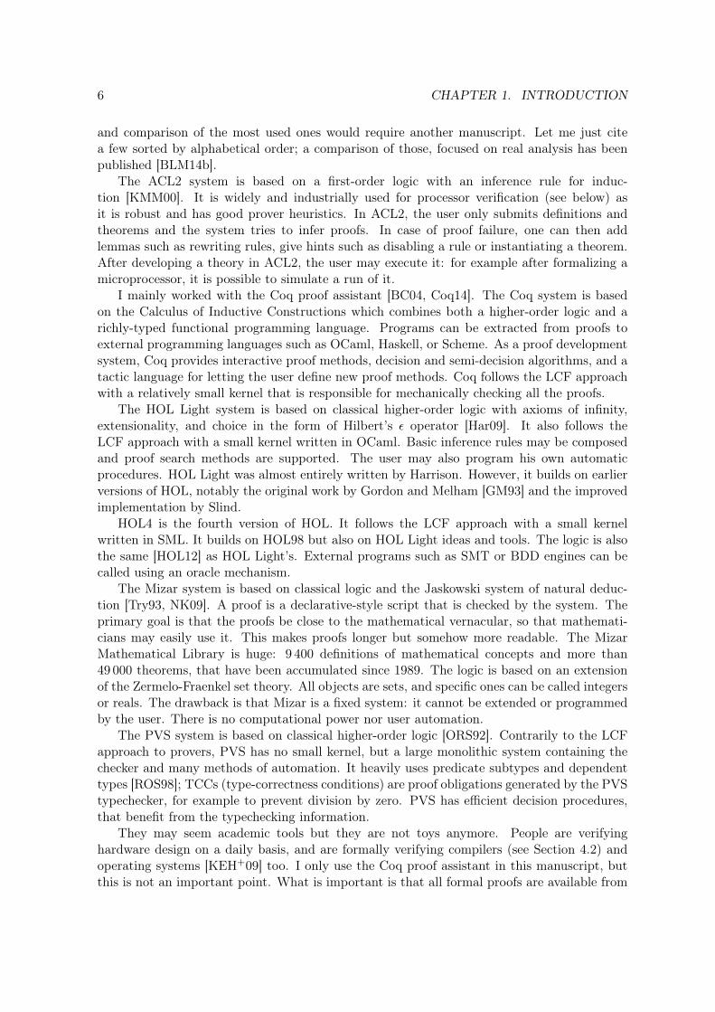
The Antikythera Mechanism is a Greek device that dates from the 1st century BC [EF11,Edm13]. Found in 1900 by sponge divers, its remaining fragments were recently subjectedto microfocus X-ray tomography and a bunch of software, including DNA matching. It wasdiscovered its purpose was astronomical: it was a calendar with the position of the Sunand Moon, eclipse prediction, and probably the position of other planets and stars. Thisastronomical calculator was made of 30 toothed bronze gears wheels and several dials. Itwas a case approximately 34 × 20 × 10 cm. Its upper-back dial was found to be a 235-month calendar, as 235 lunar months correspond almost exactly to 19 years. The AntikytheraMechanism was also able to predict possible lunar or solar eclipses, as observations show thateclipses happen 223 months later than another eclipse. A photo of a fragment and a replicaare given in Figure 1.1 and a diagram showing the complexity is in Figure 1.2. Even a Legoreplica has been set up1.

The first mechanical computers such as the Antikythera Mechanism (80-60 BC), Pas-cal’s calculator (1642), and Babbage’s machines (1830) were all mechanical computers. Thenfloating-point appeared. The first electro-mechanical computers were those made by KonradZuse (1930s and 40s) including the famous Z3. Later came the well-known Crays (1970s).Now John and Jane Doe have a computer and a smartphone, able to perform more than 109

1http://www.youtube.com/watch?v=RLPVCJjTNgk

1

http://www.youtube.com/watch?v=RLPVCJjTNgk

2 CHAPTER 1. INTRODUCTION

Figure 1.1: The Antikythera Mechanism: Photo of the A fragment on the left, Replica onthe right. From http://en.wikipedia.org/wiki/Antikythera_mechanism.c©Marsyas / Wikimedia Commons / CC BY

Figure 1.2: The Antikythera Mechanism: gear chain diagram for the known elements of themechanism. Hypothetical gears in italics.From http://en.wikipedia.org/wiki/Antikythera_mechanism.c©Lead holder / Wikimedia Commons / CC BY

FP computations per second. The (known) top supercomputer in November 20132 is Tianhe-2, developed by China’s National University of Defense Technology, with a performance of33 × 1015 FP computations per second, with more than 3,000,000 cores. Such a supercom-puter can therefore compute more than 1023 bits of FP results in one day. Tucker [Tuc11]therefore has a valid question: “Are we just getting the wrong answers faster?”.

2http://www.top500.org

http://en.wikipedia.org/wiki/Antikythera_mechanism

http://en.wikipedia.org/wiki/Antikythera_mechanism

http://www.top500.org

1.2. FLOATING-POINT ARITHMETIC 3

1.2 Floating-Point Arithmetic

Let us dive into computer arithmetic. As in Konrad Zuse’s Z3, nowadays computers usefloating-point numbers. Which numbers and how operations behave on them is standardizedin the IEEE-754 standard [IEE85] of 1985, which was revised in 2008 [IEE08].

We adopt here the level 3 vision of the standard: we do not consider bit strings, but therepresentation of floating-point data. The format will then be (β, p, emin, emax), where eminand emax are the minimal and maximal unbiased exponents, β is the radix (2 or 10), and p isthe precision (the number of digits in the significand).

In that format, a floating-point number is then either a triple (s, e,m), or an exceptionalvalue: ±∞ or a NaN (Not-a-Number). For non-exceptional values, meaning the triples, wehave additional conditions: emin ≤ e ≤ emax and the significand m has less than p digits. Thetriple can be seen as the real number with value

(−1)s ×m× βe.

We will consider m as an integer and we therefore require that m < βp. The otherpossibility is that m is a fixed-point number smaller than β. In this setting, the commonIEEE-754 formats are binary64, which corresponds to (2, 53, −1074, 971) and binary32,which corresponds to (2, 24, −149, 104).

Infinities are signed and they have mathematical meaning (and will have in the computa-tions too). The NaNs (Not-a-Numbers) are answers to impossible computations, such as 0/0or +∞− +∞. They propagate in any computation involving a NaN. As infinities, they willbe prevented in this manuscript: we will prove their absence instead of using or suffering fromthem.

Non-exceptional values give a discrete finite set of values, which can be represented on thereal axis as in Figure 1.3. FP numbers having the same exponent are in a binade and are atequal distance from one to another. This distance is called the unit in the last place (ulp) asit is the intrinsic value of the last bit/digit of the significand of the FP number [MBdD+10].When going from one binade to the next, the distance is multiplied by the radix, which givesthis strange distribution. Around zero, we have the numbers having the smallest exponentand small mantissas, they are called subnormals and their ulp is that of the smallest normalnumber.

0 R

subnormals binade (common exponent)

Figure 1.3: Distribution of the FP numbers over the real axis.

FP arithmetic tries to mimic real arithmetic but, in many cases, the exact result of anoperation on two FP numbers is not a FP number (this will often be the case in this manuscript,but this is not representative). For example, in binary64, 1 and 2−53 are FP numbers, but1 + 2−53 is not, as it would require 54 bits for the significand. The value therefore needs tobe rounded. The IEEE-754 standard defines 5 rounding modes: towards positive, towards


negative, towards zero, rounding to nearest ties to even, and rounding to nearest ties awayfrom zero.

The main rule of the IEEE standard of FP computation for basic operations is the fol-lowing one, called correct rounding: each operation gives the same result as if it was firstperformed with infinite precision, and then rounded to the desired format. This is a verystrong mathematical property that has several essential consequences:

• portability: as there is only one allowed result for an operation, you may change theprocessor, the programming language or the operating system without any change onthe result. This is called recently “numerical reproducibility”.

• accuracy: the error between the exact value and the computed value is small comparedto these values. It is bounded by one ulp for directed rounding modes and half an ulpfor roundings to nearest.

In particular, if we consider a format (β, p, emin, emax) with integer significand, then thiserror bound can be stated for any rounding to nearest ◦:

∀x, |x| ≥ βp−1+emin ⇒ |◦(x)− x| ≤ β1−p

2|◦(x)|

∀x, |x| < βp−1+emin ⇒ |◦(x)− x| ≤ βemin

2

For directed rounding modes, the same formulas apply without the division by two. Correctrounding gives other interesting properties:

• It paves the way for mathematical proofs of what is happening in a computer program.A clear semantics is needed to build proofs that correspond to reality. A clean uniquemathematical definition is therefore an advance towards safety.

• If the exact mathematical result of a computation fits in a FP format, then it is thereturned result. This property will be thoroughly used in this manuscript. If we areable to prove that the result of a computation can be represented as a FP number, thatis to say it fits in the destination format, then there will be no rounding, which is quiteuseful for the rest of the proof (such as bounding rounding error or proving algebraicequality).

• It helps to preserve some mathematical properties. For example, as both the squareroot and the rounding are increasing, the rounded square root is also increasing. An-other example is: if a function is both correctly rounded and periodic, then its roundedcounterpart is also periodic.

These properties only apply if the basic functions/operators are correctly rounded. Inpractice, this is required for addition, subtraction, multiplication, division, and square root.For these operators, three additional digits are enough to guarantee this correct rounding forall rounding modes, the last one being a sticky bit [Gol91]. Another operator available onrecent processors is the FMA (fused multiply-and-add): it computes a× x+ b with only onefinal rounding instead of a rounded multiplication followed by a rounded addition. Correctrounding is recommended for a larger set of functions, including pow, exp, sin, and cos, butit is known to be much more difficult to ensure [DDDM01].

1.3. FORMAL PROOF ASSISTANTS 5

For some ugly details, as for the difference between signaling and quiet NaNs, the signof 0 − 0 or the value of

(√−0), we refer the reader directly to the standard [IEE08]. Other

major references are an article by Goldberg [Gol91] and the Handbook of Floating-PointArithmetic [MBdD+10].

Previously, I write that this manuscript was about floating-point computations. This isnot true. This manuscript is about trust.

1.3 Formal Proof Assistants

If an article or someone tells you something is true (such as a theorem, an algorithm, aprogram), will you believe it? This question is more sociological than scientific [DLP77]. Youmay believe it for many different reasons: because you trust the author, because the resultseems reasonable, because everybody believes it, because it looks like something you alreadybelieve, because you read the proof, because you tested the program, and so on. We all havea trust base, meaning a set of persons, theorems, algorithms, programs we believe in. But weall have a different trust base, so to convince as many people as possible, you have to reducethe trust base as much as possible.

Proofs are usually considered as an absolute matter, and mathematicians are those that candiscover these absolute facts and show them. However, mathematicians do fail. An old bookof 1935 makes an inventory of 500 errors sometimes made by famous mathematicians [Lec35].Given the current publication rate, such an inventory would now take several bookshelves.As humans are fallible, how can we make proofs more reliable? A solution is to rely on aless-fallible device, the computer, to check the proofs. We also need to detail the proofs muchmore than what mathematicians usually do.

We will need a “language of rules, the kind of language even a thing as stupid as a computercan use” (Porter) [Mac04]. Formal logic studies the languages used to define abstract objectssuch as groups or real numbers and reason about them. Logical reasoning aims at checkingevery step of the proof. It then removes any unjustified assumption and ensures that onlycorrect inferences are used. The reasoning steps that are applied to deduce from a propertybelieved to be true a new property believed to be true are called an inference rule. They areusually handled at a syntactic level: only the form of the statements matters, their contentdoes not. For instance, the modus ponens rule states that, if both properties “A” and “if Athen B” hold, then property “B” holds too, whatever the meaning of A and B. To check thesesyntactic rules are correctly applied, a thing as stupid as a computer can be used. It will beless error-prone and faster than a human being, as long as the proof is given in a languageunderstandable by the computer. The drawback is that all the proof steps will need to besupported by evidence. Depending on your trust base, there are two different approaches.The first one follows the LCF approach [Gor00], meaning the only thing to trust is a smallkernel that entirely checks the proof. The rest of the system, such as proof search, may bebug-ridden as each proof step will ultimately be checked by the trusted kernel. In this case,the proof must be complete: there is no more skipping some part of the proof for shortening orlegibility. Another approach is to trust the numerous existing tools in automated deduction,such as SMT solvers (see also Section 2.2).

Many formal languages and formal proof checkers exist. For the sociological and historicalaspects of mechanized proofs, we refer the reader to MacKenzie [Mac04]. The description


and comparison of the most used ones would require another manuscript. Let me just citea few sorted by alphabetical order; a comparison of those, focused on real analysis has beenpublished [BLM14b].

The ACL2 system is based on a first-order logic with an inference rule for induc-tion [KMM00]. It is widely and industrially used for processor verification (see below) asit is robust and has good prover heuristics. In ACL2, the user only submits definitions andtheorems and the system tries to infer proofs. In case of proof failure, one can then addlemmas such as rewriting rules, give hints such as disabling a rule or instantiating a theorem.After developing a theory in ACL2, the user may execute it: for example after formalizing amicroprocessor, it is possible to simulate a run of it.

I mainly worked with the Coq proof assistant [BC04, Coq14]. The Coq system is basedon the Calculus of Inductive Constructions which combines both a higher-order logic and arichly-typed functional programming language. Programs can be extracted from proofs toexternal programming languages such as OCaml, Haskell, or Scheme. As a proof developmentsystem, Coq provides interactive proof methods, decision and semi-decision algorithms, and atactic language for letting the user define new proof methods. Coq follows the LCF approachwith a relatively small kernel that is responsible for mechanically checking all the proofs.

The HOL Light system is based on classical higher-order logic with axioms of infinity,extensionality, and choice in the form of Hilbert’s ε operator [Har09]. It also follows theLCF approach with a small kernel written in OCaml. Basic inference rules may be composedand proof search methods are supported. The user may also program his own automaticprocedures. HOL Light was almost entirely written by Harrison. However, it builds on earlierversions of HOL, notably the original work by Gordon and Melham [GM93] and the improvedimplementation by Slind.

HOL4 is the fourth version of HOL. It follows the LCF approach with a small kernelwritten in SML. It builds on HOL98 but also on HOL Light ideas and tools. The logic is alsothe same [HOL12] as HOL Light’s. External programs such as SMT or BDD engines can becalled using an oracle mechanism.

The Mizar system is based on classical logic and the Jaskowski system of natural deduc-tion [Try93, NK09]. A proof is a declarative-style script that is checked by the system. Theprimary goal is that the proofs be close to the mathematical vernacular, so that mathemati-cians may easily use it. This makes proofs longer but somehow more readable. The MizarMathematical Library is huge: 9 400 definitions of mathematical concepts and more than49 000 theorems, that have been accumulated since 1989. The logic is based on an extensionof the Zermelo-Fraenkel set theory. All objects are sets, and specific ones can be called integersor reals. The drawback is that Mizar is a fixed system: it cannot be extended or programmedby the user. There is no computational power nor user automation.

The PVS system is based on classical higher-order logic [ORS92]. Contrarily to the LCFapproach to provers, PVS has no small kernel, but a large monolithic system containing thechecker and many methods of automation. It heavily uses predicate subtypes and dependenttypes [ROS98]; TCCs (type-correctness conditions) are proof obligations generated by the PVStypechecker, for example to prevent division by zero. PVS has efficient decision procedures,that benefit from the typechecking information.

They may seem academic tools but they are not toys anymore. People are verifyinghardware design on a daily basis, and are formally verifying compilers (see Section 4.2) andoperating systems [KEH+09] too. I only use the Coq proof assistant in this manuscript, butthis is not an important point. What is important is that all formal proofs are available from

1.4. STATE OF THE ART 7

my web page3, so that they can be re-run to increase your trust in my statements.Finally, I have often been asked this question: “are you very sure?”. This can be restated

as what trust can you put in a formal system, or as who checks the checker [Pol98]. As faras I am concerned, I have no strong belief in the absolute certainty of formal systems, I havea more pragmatic point of view, influenced by Davis [Dav72] with this nice title: “Fidelity inMathematical Discourse: Is One and One Really Two?”. It describes “Platonic mathematics”and its beliefs. In particular, Platonic mathematics assume that symbol manipulation isperfect. Davis thinks this manipulation is in fact wrong with a given probability. Thisprobability depends if the manipulation is done by a human (≈ 10−3) or a machine (≈ 10−10).A cosmic ray may indeed mislead a computer to accept an incorrect proof. The probability istiny, but nonzero. My opinion is that the computer is used here to decrease the probabilityof failure, and hence increase the trust. Perfection is not achievable, we are therefore lookingfor a strong guarantee that can be achieved using formal proof assistants.

1.4 State of the Art

1.4.1 Formal Specification/Verification of Hardware

A first subject where formal proofs have been applied is the verification of hardware and, inparticular, the verification of the Floating-Point Unit (FPU). This is a logical consequenceof the Pentium bug [Coe95]: the poor publicity was very strong and all hardware makerswanted to make sure this would never happen again. Formal methods are also useful as theimplementation of computations with subnormal numbers is difficult [SST05].

Even before, formal methods have been applied to the IEEE-754 standard, and firstlyby specifications: what does this standard in English really mean? Barrett wrote a such aspecification in Z [Bar89]. It was very low-level and included all the features. Later, Minerand Carreño specified the IEEE-754 and 854 standards in PVS and HOL [Car95, Min95,CM95]. To handle similarly radixes 2 and 10, the definitions are more generic and not aslow-level. The drawback is that few proofs have been made in this setting, except by Minerand Leathrum [ML96], and this casts a doubt on the usability of the formalization.

Concerning proofs made by processor makers, AMD researchers, particularly Russinoff,have proved in ACL2 many FP operators mainly for the AMD-K5 and AMD-K7 chips [MLK98,Rus98, Rus99, Rus00]. This is an impressive amount of proofs. The square root of the IBMPower4 chip [SG02] and a recent IBM multiplier have been verified using ACL2 too [RS06].More recently, the SRT quotient and square root algorithms have been verified with a focuson obtaining small and correct digit-selection tables in ACL2 [Rus13]. This last work alsoshows that there are several mistakes in a previous work by Kornerup [Kor05].

During his PhD, Harrison verified a full implementation of the exponential function [Har97,Har00a, Har00b]. He therefore developed a rather high-level formalization of FP arithmeticin HOL Light with the full range of FP values [Har99]. Then Intel hired him and has kepton with formal methods. The Pentium Pro operations have been verified [OZGS99]. ThePentium 4 divider has been verified in the Forte verification environment [KK03]. A full proofof the exponential function, from the circuit to the mathematical function was achieved usingHOL4 [AAHTH10].

3http://www.lri.fr/~sboldo/research.html

http://www.lri.fr/~sboldo/research.html


Now for a few academic works. A development by Jacobi in PVS is composed of botha low-level specification of the standard and proofs about the correctness of floating-pointunits [Jac01, Jac02]. This has been implemented in the VAMP processor [JB05]. An appealingmethod mixes model checking and theorem proving to prove a multiplier [AS95]. Another workproves SRT division circuits with Analytica, a tool written in Mathematica [CGZ99]. A nicesurvey of hardware formal verification techniques, and not just about FP arithmetic, has beendone by Kern and Greenstreet [KG99].

1.4.2 Formal Verification of Floating-Point Algorithms

This is a short section as rather few works mix FP arithmetic and formal proofs. As men-tioned below, Harrison has verified algorithms using HOL Light. With others, he has alsodeveloped algorithms for computing transcendental functions that take into account the hard-ware, namely IA-64 [HKST99]. Our work in Coq is detailed in Sections 2.3.1 and 2.3.2.

Some additional references are related to FP arithmetic without being directly FP algo-rithms. To compute an upper bound for approximation errors, that is to say the differencebetween a function and its approximating polynomial, the Sollya tool generates HOL Lightproofs based on sum-of-squares [CHJL11]. The same problem has been studied in Coq us-ing Taylor models [BJMD+12]. Taylor models were also studied for the proof of the KeplerConjecture [Zum06].

1.4.3 Program Verification

To get a viewpoint about programs, I refer the reader to the very nice http://www.informationisbeautiful.net/visualizations/million-lines-of-code/ to see howmany lines of code usual programs contain. For example, a pacemaker is less than a hundredthousand lines; Firefox is about 10 million lines; Microsoft Office 2013 is above 40 million linesand Facebook is above 60 million lines. An average modern high-end car software is about100 million lines of code.

It is therefore not surprising to see so many bugs, even in critical applications: off-shore platform, space rendezvous, hardware division bug, Patriot missile, USS Yorktown soft-ware, Los Angeles air control system, radiotherapy machine and many others in MacKenzie’sbook [Mac04]. Research has been done and many methods have been developed to preventsuch bugs. The methods considered here mainly belong to the family of static analysis, mean-ing that the program is proved without running it.

Abstract Interpretation

The main intuition behind abstract interpretation is that we do not need to know the exactstate of a program to prove some property: a conservative approximation is sufficient. Thetheory was developed by Cousot and Cousot in the 70s [CC77]. I will only focus on staticanalysis tools with a focus on floating-point arithmetic.

Astrée is a C program analyzer using abstract interpretation [CCF+05]. It automaticallyproves the absence of runtime errors. It was successfully applied to large embedded avion-ics software generated from synchronous specifications. It uses some domain-aware abstractdomains, and more generally octagons for values and some linearization of round-off errors.

Fluctuat is a tool based on abstract interpretation dedicated to the analysis of FP pro-grams [GP06]. It is based on an affine arithmetic abstract domain and was successfully applied

http://www.informationisbeautiful.net/visualizations/million-lines-of-code/

http://www.informationisbeautiful.net/visualizations/million-lines-of-code/


to avionics applications [DGP+09]. It was recently improved towards modularity [GPV12] andto handle unstable tests [GP13].

Another tool called RAICP and based on Fluctuat manages the mix of Fluctuat andconstraint programming. Constraint programming is sometimes able to refine approximationswhen abstract interpretation is not [PMR14].

A related work, but less convincing, concerns the estimation of errors in programs writtenin Scala [DK11]. It is based on affine arithmetic too and includes non-linear and transcendentalfunctions. But all input values must be given to estimate the error of an execution, which israther limited.

Deductive Verification

Taking the definition from Filliâtre [Fil11], deductive program verification is the art of turningthe correctness of a program into a mathematical statement and then proving it.

The first question is that of defining the correctness of a program. In other words, whatis the program supposed to do and how can we express it formally? This is done using aspecification language. This is made of two parts: a mathematical language to express thespecification and its integration with a programming language. The use of a specification lan-guage is needed by deductive verification, but can also be used for documenting the programbehavior, for guiding the implementation, and for facilitating the agreement between teams ofprogrammers in modular development of software [HLL+12]. The specification language ex-presses preconditions, postconditions, invariants, assertions, and so on. This relies on Hoare’swork [Hoa69] introducing the concept known today as Hoare triple. In modern notation, ifP is a precondition, Q a postcondition and s a program statement, then the triple {P}s{Q}means that the execution of s in any state satisfying P must end in a state satisfying Q. If sis also required to terminate, this is total correctness, the opposite being partial correctness.Modern tools use weakest preconditions [Dij75]: given s and Q, they compute the weakestrequirement over the initial state such that the execution of s will end up in a final statesatisfying Q. There is left to check that P implies this weakest requirement. These tools arecalled verification condition generators and efficient tools exist.

The ACSL specification language for C and the Why3 verification condition generator willbe described in the next chapter. As for the others, we will sort them by input language.

Another C verification environment is VCC [CDH+09]. It is designed for low-level concur-rent system code written in C. Programs must be annotated in a language similar to ACSL andare translated into an intermediate language called Boogie. VCC includes tools for monitoringproof attempts and constructing partial counterexample executions for failed proofs. It wasdesigned to verify the Microsoft Hyper-V hypervisor. A hypervisor is the software that sitsbetween the hardware and one or more operating systems; the Microsoft Hyper-V hypervisorconsists of 60,000 lines of C and assembly code.

Java programs can be annotated using JML, a specification language common to numeroustools [BCC+05]. It has two main usages: the first usage is runtime assertion checking and test-ing: the assertions are executed at runtime and violations are reported. This also allows unittesting. The second usage is static verification. JML supports FP numbers and arithmetic, butno real numbers are available in the specification language. It has also been noted that NaNswere a pain as far as specification are concerned [Lea06]. Several tools exist, with differentdegrees of rigor and automation. ESC/Java2 automatically gives a list of possible errors, suchas null pointer dereferencing. KeY also generates proof obligations to be discharged by its own


prover integrating automated and interactive proving [ABH+07, BHS07]. A limit is that theuser cannot add his own external decision procedures. Jahob is the tool nearest to those usedhere: it allows higher-order specifications and calls to a variety of provers, both automaticand interactive (Isabelle and Coq). Nevertheless, its philosophy is that interactive proversshould not be used: Jahob provides various constructions, such as instantiating lemmas orproducing witnesses, to help automated provers. The idea is to have a single environment forprogramming and proving, but this means heavy annotations (even longer than ours) in theintegrated proof language [ZKR09]. Some tools, such as KeY, have the Java Card restrictionsand therefore do not support FP arithmetic.

VeriFast is a separation logic-based program verifier for both Java and C programs. Theuser writes annotations, that are automatically proved using symbolic execution and SMTprovers. Its focus is on proving safety properties, such as the absence of memory safety bugsand of race conditions. It has found many such bugs on industrial case studies [PMP+14].

Spec# is an object-oriented language with specifications, defined as a superset ofC# [BLS05]. Spec# makes both runtime checking and static verification available, the latestbeing based on the Boogie intermediate language. However, Spec# lacks several constructs:mathematical specification, ghost variables. Moreover, quantifiers are restricted to the onesthat are executable.

Dafny is both an imperative, class-based language that supports generic classes and dy-namic allocation and a verifier for this language [Lei10, HLQ12]. The basic idea is that thefull verification of a program’s functional correctness is done by automated tools. The specifi-cation language also includes user-defined mathematical functions and ghost variables. As inVCC and Spec#, Dafny programs are translated into an intermediate language called Boogie.To be executed, the Dafny code may be compiled into .NET code.

The B method uses the same language in specification, design, and program. It dependson set theory and first-order logic and is based on the notion of refinement [Abr05]. It wasdesigned to verify large industrial applications and was successfully applied to the Paris MétroLine 14.

A last work has been done on a toy language with a focus on FP arithmetic [PA13]. As inJML, no real numbers are available and rounding does occur in annotations. The specificationlanguage focuses on the stability of computations, but this only means that the computationbehaves as in extended precision. This unfortunately means neither that the computation isalways stable, nor that it is accurate.

Complementary Approaches

This section describes other approaches that are not directly related to program verification,but have other advantages.

First, interval arithmetic is not a software to verify a program, but a modification ofa program. Instead of one FP number, we keep an upper and a lower bound of the realvalue. Taking advantage of the directed roundings, it is possible to get a final interval thatis guaranteed to contain the correct mathematical value. The final interval may be useless,such as (−∞,+∞), but the motto is “Thou shall not lie”. Large intervals may be due toinstability or to the dependency problem. Nevertheless, interval arithmetic is fast and able toprove mathematical properties [Tuc99].

Test is a common validation method, but is seldom used in FP arithmetic as a completeverification method. The reason is very simple: it rapidly blows up. Consider for example a


function with only three binary64 inputs. There are 2192 possibilities. If each possibility takes1 millisecond to check, an exhaustive test requires more than 1047 years. This has neverthelessbeen used for the table maker’s dilemma for one-input functions, using smart filters andoptimizations [LM01]. Another work involves automatic test and symbolic execution: it triesto find FP inputs in order to test all execution paths [BGM06].

Another interesting approach is that of certificates: instead of proving a priori that aprogram is correct, the program generates both a result and an object that proves the cor-rectness of the result. An a posteriori checking is needed for all calls to the function, but it isvery useful in many cases. A good survey has been done by McConnell et al. [MMNS11], butthe FP examples are not convincing. It seems FP computations are not well-matched withcertificates.

An interesting recent work uses dynamic program analysis to find accuracy prob-lem [BHH12]. As in [PA13], the idea is only to compare with a higher precision, here 120bits. Besides from being slow, this does not really prove the accuracy of the result; it onlydetects some instabilities.

An orthogonal approach is to modify the program into an algebraically equivalent pro-gram, only more accurate. This has been done using Fluctuat and a smart data structurecalled Abstract Program Expression Graph (APEG) so that it is not required to exhaustivelygenerate all possible transformations in order to compare them [IM13].

Most previous approaches overestimate round-off errors in order to get a correct bound.Using a heuristic search algorithm, it is possible to find inputs that create a large floating-pointerror [CGRS14]. It will not always produce the worst case, but such a tool could validate theobtained bounds to warrant they are not too much overestimated.

1.4.4 Numerical Analysis Programs Verification

One of my application domains is numerical analysis. Here are some previous works regardingthe verification of such algorithms/programs.

Berz and Makino have developed rigorous self-verified integrators for flows of ODEs (Ordi-nary Differential Equations) based on Taylor models and differential algebraic methods, thatare the base of the COSY tool. Some current applications of their methods include provingstability of large particle accelerators, dynamics of flows in the solar system, and computerassisted proofs in hyperbolic dynamics [BM98, BMK06].

A comparable work about the integration of ODEs uses interval arithmetic and Taylormodels [NJN07]; it is also a good reference for verified integration using interval arithmetic.

Euler’s method is embedded in the Isabelle/HOL proof assistant using arbitrary-precisionfloating-point numbers [IH12, Imm14]. The Picard operator is used for solving ODEs in Coqusing constructive reals [MS13].

Outline After this introduction, the methods and tools used afterwards are described inChapter 2. The biggest chapter is then Chapter 3: it presents a gallery of formally verified Cprograms. All programs are motivated, then both data about the proofs and the full annotatedC code are given. Chapter 4 emphasizes compilation issues and several solutions. Conclusionsand perspectives are given in Chapter 5.

2. Methods and Tools for Floating-Point Program Verification

Here is the programming by contract method for verifying a C program, that can also befound in Figure 2:

• annotate the program: in C special comments, write what the program expects (suchas a positive value, an integer smaller than 42) and what the program ensures (suchas a result within a small distance of the expected mathematical value). You may alsowrite assertions, loop variants (to prove termination), and invariants (to handle what ishappening inside loops).

• generate the corresponding verification conditions (VCs): here I use Frama-C, its Jessieplugin, and Why. This chain acts as a program that takes the previous C program asinput and generates a bunch of theorems to prove. If all the theorems are proved, thenthe program is guaranteed to fulfill its specification and not to crash (due to exceptionalbehaviors, out-of-bound accesses, and so on).

• prove the VCs. This can be done either automatically or interactively using a proofassistant.

In practice, this is an iterative process: when the VCs are impossible to prove, we modifythe annotations, for example strengthen the loop invariant, add assertions or preconditions,until everything is proved.

Note that the first step is critical: if you put too many preconditions (ultimately false),then the function cannot be reasonably used; if you put too few postconditions (ultimatelytrue), then what you prove is useless. This is not entirely true, as a proved empty postconditionmeans at least that there is no runtime error, which is an interesting result per se.

Let us go into more details. This chapter is divided into three sections. Section 2.1describes the annotation language and the resulting VCs. Section 2.2 introduces the provers.Section 2.3 presents the formalizations of floating-point arithmetic for interactive provers.Section 2.4 describes a Coq library for real analysis.

2.1 Annotation Language and Verification Conditions forFloating-Point Arithmetic

An important work is the design of the annotation language for floating-point arith-metic [BF07]. The goal is to write annotations that are both easy to understand and useful.First, I need to convince the reader of what is proved. Therefore the language must be under-standable to those who are not experts in formal methods: I want computer arithmeticians tounderstand what is proved from the annotations. Second, I need people to use the annotations.Therefore they must correspond to what they want to guarantee on programs.

13

14 CHAPTER 2. METHODS AND TOOLS FOR FP PROGRAM VERIFICATION

Annotated C Program(specification, invariant) Human

Verification Conditions(Theorem statements)

Frama-CJessie plugin

Why

Alt-Ergo CVC3 Z3 Gappa Coq

HumanProved VCs

The program is correct withrespect to its specification

Figure 2.1: Scheme for verifying a C program. Red means the need for human interaction.

2.1. ANNOTATION LANGUAGE AND VC FOR FP ARITHMETIC 15

With Filliâtre, I first designed this language for Caduceus [FM04, FM07]. Caduceus is atool for the static analysis of C programs using a weakest precondition calculus developed byFilliâtre and Marché. Then Caduceus was superseded by Frama-C [CKK+12]: it is a frame-work that takes annotated C as input. The annotation language is called ACSL (for ANSI/ISOC Specification Language) [BCF+14a] and is quite similar to JML: it supports quantifiers andghost code [FGP14] (model fields and methods in JML) that are for specification only, andtherefore not executed. Numerous Frama-C plugins are available for different kinds of analysissuch as value analysis using abstract interpretation, browsing of the dataflow, code transfor-mation, and test-case generation. I use deductive verification based on weakest preconditioncomputation techniques. The available plugins are WP and Jessie [Mar07].

The annotation language for floating-point arithmetic was directly taken from Caduceusto Frama-C. The choice is to consider a floating-point number f as a triple of three values:

• its floating-point value: what you really have and compute with in your computer. Forintuitive annotations, this value is produced when f is written inside the annotations.

• its exact value, denoted by \exact(f). It is the value that would have been obtained ifreal arithmetic was used instead of floating-point arithmetic. It means no rounding andno exceptional behavior.

• its model value, denoted by \model(f). It is the value that the programmer intendsto compute. This is different from the previous one as the programmer may want tocompute an infinite sum or have discretization errors.

A meaningful example is that of the computation of exp(x) for a small x. The floating-point value is 1+x+x*x/2 computed in binary64, the exact value is 1 +x+ x2

2 and the modelvalue is exp(x). This allows a simple expression of the rounding error: |f − \exact(f)| andof the total error. An important point is that, in the annotations, arithmetic operations aremathematical, not machine operations. In particular, there is no rounding error. Simplyspeaking, we can say that floating-point computations are reflected within specifications asreal computations.

Time has shown that the exact value is very useful. It allows one not to state again partof the program in the annotations, which is quite satisfactory. This idea of comparing FPwith real computations is caught again by Darulova and Kuncak [DK14]. As for the modelvalue, this is not so clear: people need to express the model part, but they do not use themodel value for it. They define the intended value as a logical function and compare it to thefloating-point result. In my opinion, the reason is mostly sociological: the annotations thenclearly state what the ideal value is. When the model part is set somewhere in the program,it is less convincing. A solution is to express the value of the model part as a postcondition,but it makes the annotations more cumbersome.

The C annotated program is then given to Frama-C and its Jessie plugin. They transformit into an intermediate language called Why. FP numbers and arithmetic are not built-inin Why. The floating-point operations need to be specified in this intermediate language togive meaning to the floating-point operations. This description is twofold. First, it formalizesthe floating-point arithmetic with a few results. For example, the fact that all binary64roundings are monotonic is stated as follows.


axiom round_double_monotonic :f o ra l l x , y : real . f o ra l l m:mode .x <= y −> round_double(m, x ) <= round_double(m, y )

This is an axiom in Why, but all such axioms are proved in Coq using the formalizationsdescribed in Section 2.3. This is used by automatic provers, even if they know nothing aboutFP arithmetic.

The second part of the description is the formalization of floating-point operations. Forinstance, the addition postcondition states that, if there is no overflow, the floating-point valueis the rounding of x + y, the exact part is the exact addition of the exact parts of x and y,and similarly for the model part.

There is a choice here: by default, we want to prove that no exceptional behaviors occurs.This means that every addition creates a VC that requires that it does not overflow, andsimilarly for subtraction, multiplication, and division (with another for the fact that the divisoris non-zero). The idea is to absolutely prevent exceptional behavior. An extension has beendone that allows exceptional values and computations on them [AM10]. It can be useful insome cases as computations with infinities is quite reasonable, but it means more possibilitiesfor each computation. Therefore, interactive proofs become incredibly cumbersome. Moreover,our choice implies that inputs of functions cannot be infinities or NaNs. This removes theproblems of NaN inputs in annotations described by Leavens [Lea06].

Using weakest preconditions computations, VCs are generated corresponding to FP re-quirements and giving FP properties. Why is then able to translate a VC, meaning a logicalstatement into the input language of many provers described in the next section.

There is a subtlety here as two different Why tools are used. First Why2 (that is to sayWhy 2.x) [Fil03, FM04] is used in most programs. It has a limited ability to call interactiveprovers (such as Coq or PVS). In this case, all VCs are put into a single file. It means that ifVCs 1, 3, and 4 are proved with an automatic prover, but 2 and 5 require interactive proofs,Why2 generates a single file with all 5 VCs. If the user does not want to interactively prove1, 3, and 4, he may remove it from his file so that only 2 and 5 are left. This is the case onlyin the example of Section 3.9. But there is no check by an automatic tool that this removingis safe. The next version is Why3 [Fil13] that allows to use a prover on a VC and to checkindependently the correctness of each VC [BFM+13]. There is therefore no manual removingand this increases the guarantee. Why2 and Why comes with a graphical interface to call anyprover on any VC. A screenshot is given in Figure 2.2.

Why3 files include declaration of types and symbols, definitions, axioms, and goals. Suchdeclarations are organized in small components called theories. A theory may have an axiomthat states that 0 = 1. To ensure the consistency of a theory, this theory can be realized: itmeans that definitions are given and axioms proved, using for instance an interactive prover.This is possible when using only Why3, but not when using the Frama-C/Jessie/Why3 chainfor now. This means that axiomatics defined in ACSL (such as the definition of the ulp) needWhy2 to be realized. The need for these axiomatics can be questioned, but this seemed thebest choice for readability when specifying these programs.

2.2. PROVERS 17

Figure 2.2: Snapshot of the Why3 GUI on the program of Section 3.5.

2.2 Provers

Once the VCs are computed, they must be proved. Several automated provers exist, dependingon the underlying logic and theories involved. The Why tools translate the VCs into the inputformat of the chosen solver.

The solvers that have improved the most recently are SMT solvers. SMT solvers, forSatisfiability Modulo Theories, are tools that decide if a theorem is correct or not. The logicthese solvers are based on is usually first-order classical logic, with several theories added, suchas arithmetic, tableaux, and bits vectors. The ones used here are Alt-Ergo [CCKL08, Con12],CVC3 [BT07], and Z3 [dMB08]. None of them know anything about FP arithmetic by default.This is the reason for providing them with the preceding description in Why that servesas theory. An efficient solution is bit blasting, even if it may get intractable [AEF+05].Another SMT solver is MathSat5 [HGBK12], and it has a decision procedure for FP which issmarter than bit blasting. It mainly handles ranges using conflict-driven clause learning. Notethere is a standardization of the FP arithmetic for all SMT solvers, that includes exceptionalvalues [RW10].

The prover I use the most is Gappa [DM10, dDLM11]. It is based on interval arithmeticand aims at proving properties of numerical programs, especially ranges of values and boundson rounding errors. The inputs are logical formulas quantified over real numbers. The atomsare explicit numerical intervals for expressions. Of course, rounding functions may be usedinside expressions. The user may provide hints, such as splitting on a variable, to help Gappasucceed. I use Gappa for simple proofs for overflow, for rounding errors, and for a local errorin the last program.

Gappa is not only a prover. It is also able to generate a Coq proof of the proved properties,to increase the trust in this yes/no answer. This feature has served to develop a Coq tacticfor automatically solving goals related to floating-point and real arithmetic [BFM09].

There is improvement left in these solvers as some VCs may only be proved by combiningthe features of both Gappa and SMT provers. Some work has been done to mix Gappa andAlt-Ergo [CMRI12], but it is only a prototype.


2.3 Formalizations of Floating-Point Arithmetic

When automatic provers are unable to prove the VCs, which is often the case in the describedprograms as they are tricky, we are left with interactive provers. Floating-point arithmetic isspecified in Why, but must also be formalized in the proof assistants.

While at NIA, I worked with PVS [ORS92] and I defined the high-level floating pointarithmetic formalization of the PVS NASA library [BM06] with a few applications. A low-level formalization of the IEEE-754 standard exist [Min95, CM95] and I also related both.

I mainly work with the Coq proof assistant. It comes with a standard library, so that usersdo not have to start their proofs from scratch but can instead reuse well-known theoremsthat have already been formally proved beforehand. This general-purpose library containsvarious developments and axiomatizations about sets, lists, sorting, arithmetic, real numbers,etc. Here, we mainly use the Reals standard library [May01] and we are also working on itsimprovement (see Section 2.4). A very useful tactic is Interval that simplifies the proofs ofinequalities on expressions of real numbers [Mel12].

The standard library does not come with a formalization of floating-point numbers. Forthat purpose, I have used the two libraries described below.

2.3.1 PFF

The PFF library was initiated by Daumas, Rideau, and Théry [DRT01] in 2001. After anumber of proofs during my PhD, I took over from them. I have contributed and maintainedthe library since then.

Given a radix β greater than one, a FP number x is only a record composed of two signedintegers: the mantissa nx and the exponent ex. As expected, its real value is obtained bycomputing nx × βex .

An FP format is a couple (N,Ei) of natural numbers that correspond to a bound on themantissa and to the minimal exponent. An FP number (n, e) is in the format if and only if

|n| < N and − Ei ≤ e.

In practice, N will be βp most of the time, with p being the precision of the format. Someextensions have been made to handle exceptional values (infinities and NaNs), but they wereunpractical [Bol04a]. Note that several bounded floats will represent the same real value.Consider for example in radix 2 the value: 1 = (1, 0) = (102,−1) = (1002,−2). If needed, acanonical value can be computed: it either has the minimal exponent or a mantissa greater orequal to βp−1. In practice, this was seldom used because seldom needed, except for definingthe ulp.

The main characteristic of this formalization is the fact that roundings are axiomaticallyformalized. A rounding here is a property between a real number and a FP number (asexpected, it also takes the radix and the format). Contrary to many formalizations, it is nota function from reals to FP numbers. It means in particular that there is no computationalcontent and that several FP numbers may be correct roundings of a real. Moreover, theFP number has to be given, with its proof of being one of the possible rounding. This hasadvantages: results that hold for any rounding or any rounding to nearest (whatever the tie)are easy to handle.

A drawback is the unintuitive definition of a rounding: it is a property such that any realcan be rounded; if a FP number is a rounding of a real value, then any FP number equal to

2.3. FORMALIZATIONS OF FLOATING-POINT ARITHMETIC 19

the first one also has the property of being a rounding of the real number; any rounding iseither the rounding up or down of the real number; the rounding is non-decreasing. Of course,IEEE-754 roundings are defined. Another rounding is defined that captures both possible FPnumbers when the real to round is in the middle.

Another drawback is the lack of automation: to prove that a floating-point number iscorrectly rounded is very long and tedious. These choices done, a large library was developed,with many results [Bol04b, BD01, BD02, BD03, BD04a, BD04b, Bol06a, BM08, RZBM09,BDL09, BM11b].

2.3.2 Flocq

Flocq was developed with Melquiond to supersede both PFF, the Coq library of Gappa, andInterval. This section gives the main features of the library [BM11a].

The first feature is that FP numbers are a subset F of the real numbers. This means thereis no requirement for now that F be discrete or that 0 ∈ F. It therefore removes the need fora coercion from F to R, which is rather painful in PFF.

There will be two definitions of the rounding modes: one axiomatic as before, but alsoone computable. A rounding predicate Q has the Coq type R → R → Prop. For it to be arounding predicate, it must fulfill two requirements. First, it must be total: any real can berounded. Second, it must be monotone: ∀x, y, f, g ∈ R, Q(x, f)⇒ Q(y, g)⇒ x ≤ y ⇒ f ≤ g(that is to say nondecreasing). These two properties are sufficient for a rounding predicate tohave reasonable properties. For example, those properties imply the uniqueness of rounding:two reals that are roundings of the same value are equal. This is different from PFF wherethe corresponding property was x < y ⇒ f ≤ g. Indeed, unicity is not required by PFF.

As in PFF (see above), we can then define the common rounding modes by theirmathematical properties for a given F. For instance, rounding toward −∞ is defined byf ∈ F ∧ f ≤ x ∧ (∀g ∈ F, g ≤ x⇒ g ≤ f).

F cannot just be any subset of R. Consider for example the set of rational numbers, thenan irrational number x cannot be rounded toward −∞: there is always another rational that issmaller than x and nearer to x. To define rounding to nearest, with ties to even, an additionalhypothesis on F is required, so that, among two successive FP numbers, one and only one iseven.

Representing formats as predicates and rounding modes as relations on real numbers makesit simple to manipulate them when rounded values are known beforehand. But they are apain when a proof actually needs to account for a value being the correct rounding. Thereforewe have chosen a more computational approach for another representation of formats androunding modes.

All the formats of this family (called generic format) satisfy the following two main prop-erties: they contain only floating-point numbers m · βe and all the representable numbers ina given slice are equally distributed.

The slice of a real number x is given by its discrete β-logarithm e = slice(x) such thatβe−1 ≤ |x| < βe. Then, a format Fϕ is entirely described by a function ϕ : Z → Z thattransforms numbers’ discrete logarithms into canonical exponents for this format. In otherwords, a number x is in Fϕ if and only if it can be represented as a floating-point numberm · βϕ(slice(x)).

More precisely, the format Fϕ is defined as the set of real numbers x such that x is equalto Z

(x · β−ϕ(slice(x))

)· βϕ(slice(x)) with Z the integer part (rounded toward zero).


As expected, ϕ must satisfy a few constraints in order to be a valid format with definableroundings. The common formats are fixed-point (FIX), floating-point with unbounded ex-ponents (FLX), floating-point with gradual underflow (FLT, the only available in PFF), andfloating-point with abrupt underflow (FTZ). The table below formally defines these formatsand how they can be defined using ϕ functions:

Format is defined by ∃f, F2R(f) = x ∧ . . . ϕ(e) =

FIXemin(x) ef = emin emin

FLXp(x) |nf | < βp e− pFLTp,emin(x) emin ≤ ef ∧ |nf | < βp max(e− p, emin)

FTZp,emin(x) x 6= 0⇒ emin ≤ ef ∧ βp−1 ≤ |nf | < βp{e− p if e− p ≥ emin,emin + p− 1 otherwise.

Figure 2.3 shows the graph of the corresponding ϕ functions for the three usual familiesof floating-point formats.

The ulp (unit in the last place) of a real number x is defined as βϕ(slice(x)). This functionis partial: it is not defined for 0 (neither was slice(x)). But it is defined for any other real, beit in Fϕ or not. Several developments have been done using Flocq, including some I did notcontribute to [MDMM13].

FLXFLT

FTZFTZ

FLT

FLX

ϕ(e)

emin emin + p− 1 e

emin

p− 1emin +

p

Figure 2.3: Values of ϕ for formats FLX, FLT, and FTZ, with precision p. These functionsare the same for normal numbers (e ≥ emin + p), but they diverge for subnormal numbers. Inparticular, the ϕ function for FTZ is discontinuous.

FP libraries are a base of this work, but recent applications about numerical analysis haverequired a formal library about real analysis. Coq has evolved a lot during the last decade,but the standard library for real numbers was designed more than ten years ago and has notevolved with Coq.

2.4. A REAL ANALYSIS COQ LIBRARY 21

2.4 A Real Analysis Coq Library

The limits of the standard library for real numbers was especially glaring when we considerednumerical analysis programs and especially the program solving the one-dimensional waveequation of Section 3.9. We wanted to prove that the following d’Alembert’s formula

1

2(u0(x+ ct) + u0(x− ct)) +

1

2c

∫ x+ct

x−ctu1(ξ) dξ +

1

2c

∫ t

0

∫ x+c(t−τ)

x−c(t−τ)f(ξ, τ) dξ dτ

is solution to the partial differential equation of Section 3.9 and regular enough. This wasnext to impossible using the standard library for real numbers. A reason is the overall useof dependent types: the differentiation operator takes a function f , a real number x, and aproof that f is differentiable at point x, and it returns the value of the derivative of f at x.Similarly, the integration operator requires a proof that the function is integrable. Therefore,taking the second derivative of the previous formula would have been ponderous.

With Lelay and Melquiond, we have worked to develop a user-friendly library of realanalysis. After a survey of the main proof assistants and real analysis libraries [BLM14b], wedesigned the Coquelicot library to increase the practicability for the end user [BLM14a]. Wemostly drew our inspiration from Harrison’s theory of Euclidean Space [Har13] and from theuse of filters and type classes in Isabelle/HOL [HIH13].

We provide definitions for limits, derivatives, integrals, series, and power series [LM12,BLM12]. Whenever different, these definitions are proved equivalent to those of the standardlibrary, so that user developments can easily mix both libraries. For all of those notions of realanalysis, total functions are available. These functions return the expected value in case ofconvergence and an arbitrary infinite or real number otherwise. To help with the proof process,the library comes with a comprehensive set of theorems that cover not only these notions,but also some extensions such as parametric integrals, two-dimensional differentiability, andasymptotic behaviors. A tactic to automate proofs of differentiability is also provided.

3. A Gallery of Verified Floating-Point Programs

Even a seemingly simple numerical algorithm is virtually impossible to analyzewith regards to its accuracy. To do so would involve taking into account everysingle floating-point operation performed throughout the entire computation.

Tucker [Tuc11]

This chapter presents several examples of this “virtually impossible” task: the analysis ofthe accuracy of FP programs. This is a gallery of FP programs I formally verified using thetools presented in Chapter 2. More details about the proofs can be found in the correspondingpapers especially concerning the genericity, such as if the proof holds whatever the radix andwhat is the required minimal precision. The Coq proofs for the VCs often rely on these genericprevious proofs. The size of these proofs are put into a “previous Coq proofs” line to give thereader a better order of magnitude of the full proof. The programs only use binary64 FPnumbers and rounding to nearest, ties to even. For each program, the automated provers, theamount of Coq proofs and the fully annotated C program are given after a short introduction.

The certification of these programs has lasted for years. Therefore tools are not alwaysthe same. There is nothing left using Caduceus, but some programs rely on Why3, whileothers on Why2. This is mainly for historical reasons: the programs proved long ago rely onWhy2, while the most recent ones rely on Why3. Another reason is that some results are onlyavailable in PFF and that the translation from PFF to Flocq is time-consuming.

Here is an overview of the verified programs. The first ones are basic literature floating-point algorithms: the exact subtraction, also known as Sterbenz’s theorem, and Malcolm’salgorithm to determine the radix. Then comes Dekker’s algorithm to compute the exact errorof a multiplication. Then come two algorithms by Kahan, an accurate discriminant and thearea of a triangle. The next program KB3D and its variant come from avionics. The last twoprograms come from numerical analysis: the first one is a simple linear recurrence of order 2.The last one is the biggest piece: it is a numerical scheme that solves the 1D wave equation.

As for the choice of these examples, most of them come from Goldberg’s “What everycomputer scientist should know about floating point arithmetic” [Gol91]. This has been myfavorite paper for years as it is both broad, meaning it can be read by non-specialists, anddeep, meaning that specialists may learn from it. For me, this is the reference paper thatdescribes what is the “literature” of FP arithmetic, hence my will to formally verify it.

The tool versions used are the ones available at the time this manuscript is written. Thenumber of lines of Coq proofs are given for information only as it may change when upgradingone of the tools. These programs, the list of used tools and their version numbers are availablefrom my web page1. All the Coq proofs are also given, so that all the verifications can be runagain. By default, the timings are given in seconds on a 3-GHz dual core machine.

1http://www.lri.fr/~sboldo/research.html

23

http://www.lri.fr/~sboldo/research.html

24 CHAPTER 3. A GALLERY OF VERIFIED FLOATING-POINT PROGRAMS

3.1 Exact Subtraction under Sterbenz’s Conditions

The most basic property of floating-point arithmetic is probably this one: if two FP numbersare near one to another, their subtraction is exact. Its paternity is usually given to Ster-benz [Ste74] even if Kahan also claims it. More precisely, it states that, if x and y are FPnumbers such that y

2 ≤ x ≤ 2y, then x − y is computed without error, because it fits into aFP number. This may be a benign cancellation as it is a correct computation. This may alsobe a catastrophic cancellation, as it magnifies the previous errors. Nevertheless, it is not thesubtraction that is inaccurate, even if it is often blamed for inaccuracy.

The program is put on the next page. Note that computations inside annotations areexact. Therefore, the value x-y in the postcondition is the mathematical subtraction betweenx and y. Two VCs are generated using Why2: one for the postcondition and one for safety,corresponding to the fact that there will be no FP overflow.

Proof obligations Coq TimeNb lines

VC for behavior 7VC for safety 20Total (25 lines spec VC excluded) 27 1.93

This program is also verified using Why3. The same VCs are generated, but I take advan-tage of CVC3 to automatically prove the overflow VC.

Proof obligations CVC3 CoqNb lines

VC for behavior 2.34 6VC for safety 0.23

3.1. EXACT SUBTRACTION UNDER STERBENZ’S CONDITIONS 25

/*@ requires y/2. <= x <= 2.*y;@ ensures \result == x-y;@*/

float Sterbenz(float x, float y) {return x-y;

}


3.2 Malcolm’s Algorithm

This is a program known since the 70s that computes the radix [Mal72]. This may seem astrange idea as radix 2 is now omnipresent, but this algorithm runs on any kind of architecture(including pocket calculators). If extended registers are used (see Chapter 4), this algorithmfails as explained by Gentleman and Marovich [GM74]. Note also that radix 10 is back thanksto the new IEEE-754 standard and a few CPU with radix-10 units have already appeared. Itmay give this algorithm a new boost.

The idea is to get one of the smallest positive values such that x = ◦(x + 1). Then, thesmallest FP value greater than x is x+ β. The proof of this algorithm for any radix is rathercomplicated as the values 2i may turn inexact due to rounding on radices other than powers of2. Our formalization for C programs only considers radix-2, therefore we exactly know whichand how much computations will be done. In particular, each multiplication by 2 is exact.

The result of this program is proved to be 2, but the most interesting part is the terminationof this program and its loop invariant. It may be doubtful that a while loop with conditionA != A+1 does terminate.


VC for behavior 1. loop invariant initially holds 32. loop invariant initially holds 23. loop invariant initially holds 24. loop invariant preserved 165. loop invariant preserved 26. loop invariant preserved 737. assertion 488. assertion 59. loop invariant initially holds 210. loop invariant initially holds 211. loop invariant preserved 912. loop invariant preserved 1313. postcondition 21

VC for safety 1. floating-point overflow 92. floating-point overflow 83. arithmetic overflow 14. arithmetic overflow 15. variant decreases 16. variant decreases 37. floating-point overflow 58. floating-point overflow 79. floating-point overflow 510. arithmetic overflow 111. arithmetic overflow 112. variant decreases 113. variant decreases 1

Total (1,191 lines spec VC excluded) 242 1 min 15

3.2. MALCOLM’S ALGORITHM 27

/*@ ensures \result == 2.; */

double malcolm1() {double A, B;A=2.0;/*@ ghost int i = 1; */

/*@ loop invariant A== \pow(2.,i) &&@ 1 <= i <= 53;@ loop variant (53-i); */

while (A != (A+1)) {A*=2.0;/*@ ghost i++; */

}

/*@ assert i==53 && A== 0x1.p53; */

B=1;/*@ ghost i = 1;*/

/*@ loop invariant B == i && (i==1 || i == 2);@ loop variant (2-i); */

while ((A+B)-A != B) {B++;/*@ ghost i++; */

}

return B;

}


3.3 Dekker’s Algorithm

Other algorithms from the 70s are those of Veltkamp and Dekker [Vel69, Dek71]. Veltkamp’salgorithm splits a FP number into its most significant half and its least significant part. Moreprecisely, from a p-bit FP number x, it gets its rounding on about p

2 bits that is hx = ◦ p2(x)

and the tail tx such that x = hx + tx and tx also fits in about p2 bits. The “about” is due to

the parity of p. When p is even, both hx and tx are on p2 bits. In radix 2, they both fit on⌊p

2

⌋bits as the sign of tx saves us a bit. In the other cases, hx and tx may fit on

⌊p2

⌋and

⌈p2

⌉bits (or vice versa) depending on the chosen constant C.

Then Dekker’s algorithm builds upon the previous one to compute the error of the FPmultiplication. The idea is to compute the upper and the lower parts of x and y and multiplyall the parts without rounding error. Then, the algorithm subtracts from the rounded multi-plication all the multiplied parts in the right order, i.e. from the largest to the smallest. Theresult is the correct multiplication subtracted from the rounded one, that is the error.

In order to guarantee that the multiplications of the halves are correct, we have to requirethe radix to be 2 or the precision to be even [Bol06b]. Underflow is a bit tricky to handle,as the returned value may not be the exact error anymore, but only a reasonable approxi-mation [Bol06b]. The algorithm proof provides the underflow constant 2−969. The overflowconstants are such that no overflow will happen, especially in the multiplication by C. TheseVCs are proved by the gappa tactic, hence the one-line proofs. The first requirement statesthat the input xy is equal to the correct rounding to nearest of x*y. This is for the functionto have a single FP number as a result, instead of a structure.


Previous Coq proof (spec + proof) 2,639VC for behavior 1. assertion 3

2. postcondition 238VC for safety 1. floating-point overflow 2

2. floating-point overflow 13. floating-point overflow 24. floating-point overflow 15. floating-point overflow 16. floating-point overflow 17. floating-point overflow 18. floating-point overflow 19. floating-point overflow 110. floating-point overflow 3711. floating-point overflow 4712. floating-point overflow 4313. floating-point overflow 6414. floating-point overflow 4315. floating-point overflow 8316. floating-point overflow 4917. floating-point overflow 94

Total (1,248 lines spec VC excluded) 3,351 9 min 02

3.3. DEKKER’S ALGORITHM 29

/*@ requires xy == \round_double(\NearestEven,x*y) &&@ \abs(x) <= 0x1.p995 &&@ \abs(y) <= 0x1.p995 &&@ \abs(x*y) <= 0x1.p1021;@ ensures ((x*y == 0 || 0x1.p-969 <= \abs(x*y))@ ==> x*y == xy+\result);@*/

double Dekker(double x, double y, double xy) {

double C,px,qx,hx,py,qy,hy,tx,ty,r2;C=0x8000001p0;/*@ assert C == 0x1p27+1; */

px=x*C;qx=x-px;hx=px+qx;tx=x-hx;

py=y*C;qy=y-py;hy=py+qy;ty=y-hy;

r2=-xy+hx*hy;r2+=hx*ty;r2+=hy*tx;r2+=tx*ty;return r2;

}


3.4 Accurate Discriminant

Computing a discriminant, namely b × b − a × c is known to be a FP mess. When the twosubtracted values are nearly equal, only the FP errors made during the multiplications areleft and the final error may be relatively large. A solution is the following algorithm due toKahan [Kah04]. It tests whether we are in the cancellation case or not. If not, it goes forthe naive algorithm (that is accurate enough). In case of possible cancellation, it computesthe errors of both multiplications (using the previous algorithm, with the previously givenannotations) and adds all the terms in the correct order to get an accurate result.

The tricky part lies in the test: it is supposed to clearly make apart the cancellation casesfrom the other cases. In the initial pen-and-paper proof [Kah04, BDKM06], the result of thetest was assumed to be correct, meaning as if it were computed without error. Unfortunately,this is not the case due to the multiplication by 3 and this was discovered during the formalverification of the program. Fortunately, this does not change the accuracy of the final result:in the special cases where the FP test may be wrong, we know that p + q ≈ 3 × |p − q| andtherefore b× b and a× c are about in a factor of 2. This does not suffice to apply Sterbenz’stheorem, but it does suffice to bound the cancellation and to get the same error bound, namely2 ulps.

Note that the ulp is not an ACSL primitive, and therefore needs to be axiomatized. Hereis a precise definition of the ulp: it is a power of 2, it is equal to 2−1074 for subnormals and itis such that |f | < 253ulp(f) otherwise. This set of axioms is required to guarantee that whatI call ulp is indeed the FP common value, and not a constant I put to make the proof run,such as 22000. This axiomatic is then realized in Coq to relate it to the ulp defined in Flocq.

A recent work has improved upon this accuracy using the FMA operator [JLM13].


Previous Coq proof (spec + proof) 3,390VC for theory realization 88VC for behavior 1. postcondition 61

2. postcondition 90VC for safety 1. floating-point overflow 2

2. floating-point overflow 23. floating-point overflow 34. floating-point overflow 45. floating-point overflow 46. precondition for call 27. precondition for call 98. precondition for call 19. precondition for user call 210. precondition for user call 211. precondition for user call 212. precondition for user call 213. precondition for user call 214. floating-point overflow 4415. floating-point overflow 45

Total (1,146 lines spec VC excluded) 3,655 5 min 47

3.4. ACCURATE DISCRIMINANT 31

/*@ axiomatic FP_ulp {@ logic real ulp(double f);@@ axiom ulp_normal1 :@ \forall double f; 0x1p-1022 <= \abs(f)@ ==>\abs(f) < 0x1.p53 * ulp(f);@ axiom ulp_normal2 :@ \forall double f; 0x1p-1022 <= \abs(f)@ ==> ulp(f) <= 0x1.p-52 * \abs(f);@ axiom ulp_subnormal :@ \forall double f; \abs(f) < 0x1p-1022@ ==> ulp(f) == 0x1.p-1074;@ axiom ulp_pow :@ \forall double f; \exists integer i;@ ulp(f) == \pow(2.,i);@ } */

/*@ ensures \result==\abs(f); */double fabs(double f);

/*@ requires@ (b==0. || 0x1.p-916 <= \abs(b*b)) &&@ (a*c==0. || 0x1.p-916 <= \abs(a*c)) &&@ \abs(b) <= 0x1.p510 && \abs(a) <= 0x1.p995 && \abs(c) <= 0x1.p995 &&@ \abs(a*c) <= 0x1.p1021;@ ensures \result==0. || \abs(\result-(b*b-a*c)) <= 2.*ulp(\result);@ */

double discriminant(double a, double b, double c) {double p,q,d,dp,dq;p=b*b;q=a*c;

if (p+q <= 3*fabs(p-q))d=p-q;

else {dp=Dekker(b,b,p);dq=Dekker(a,c,q);d=(p-q)+(dp-dq);

}return d;

}


3.5 Area of a Triangle

Another algorithm by Kahan computes the area of a triangle. The common formula is twomillenia old and attributed to Heron of Alexandria, but it is inaccurate for degenerated trian-gles. Kahan’s formula is mathematically equivalent, but numerically stable. There is no testneeded here, only an algebraically equivalent formula.

This was first “published” on the web [Kah86], and then published in Goldberg’s arti-cle [Gol91] with a bound of 11 ε, where ε stands for β1−p

2 that is 2−53 in binary64. My workimproved the error bound to 6.625 ε [Bol13] and I recently improved it to 4.75 ε.

It seems this example has drawn some academic attention recently. A comparable errorbound is proved, but only on very specific triangles, which are non-pathological: a = 9, b = cand 4.501 ≤ b ≤ 4.89 [DK11] and b = 4, c = 8.5 and 4.500005 ≤ a ≤ 6.5 [DK14]. In thelast case, it is additionally required that b + c > a + 10−6, in order to prove that the squareroot will not fail. I proved that this assumption is superfluous. Another work proves thatboth Kahan’s and Heron’s formula are unstable [PA13], which is correct, but does not giveany insight on the final accuracy of the result.

Proof obligations Gappa CoqNb lines

Previous Coq proof 18.89 2,091VC for behavior 16.00 82VC for safety 1. floating-point overflow 0.02

2. floating-point overflow 0.033. floating-point overflow 0.034. floating-point overflow 0.035. floating-point overflow 0.036. floating-point overflow 0.007. floating-point overflow 0.028. floating-point overflow 0.019. floating-point overflow 0.0010. floating-point overflow 0.0211. floating-point overflow 0.0212. precondition for call 13.22 1313. floating-point overflow 0.0314. floating-point overflow 0.04

3.5. AREA OF A TRIANGLE 33

/*@ requires 0 <= x;@ ensures \result==\round_double(\NearestEven,\sqrt(x));@*/

double sqrt(double x);

/*@ logic real S(real a, real b, real c) =@ \let s = (a+b+c)/2;@ \sqrt(s*(s-a)*(s-b)*(s-c));@ */

/*@ requires 0 <= c <= b <= a && a <= b + c && a <= 0x1p255;@ ensures 0x1p-513 < \result@ ==> \abs(\result-S(a,b,c)) <= (4.75*0x1p-53 + 33*0x1p-106)*S(a,b,c);@ */

double triangle (double a,double b, double c) {return (0x1p-2*sqrt((a+(b+c))*(a+(b-c))*(c+(a-b))*(c-(a-b))));

}


3.6 KB3D

This program comes from avionics. More precisely, KB3D takes as inputs the position andvelocity vectors of two aircraft. The output is a maneuver for preventing conflicts that involvesthe modification of a single parameter of the original flight path: vertical speed, heading, orground speed [DMC05, MSCD05]. This algorithm is distributed: each plane runs it simulta-neously and independently. As any avionics application, the certification level is quite high.A formal proof in PVS of the whole algorithm has been done. It is rather long even if theprogram itself is rather short. But this formal proof was done assuming correct computationson R. Unfortunately, FP inaccuracies may alter the decisions made by this algorithm.

Here, I present a small part of KB3D (rewritten in C) that decides to go on the left oron the right by computing the sign of a quantity. This is typically where FP arithmetic maymake results go wrong. The algorithm was therefore modified in order to have the followingspecification: when it gives an answer, it is the correct one. The idea is to have an errorbound on the value to be tested. If the value is over this error bound, it is sure to be positive,regardless of the errors. If the value is under the error bound, it is sure to be negative. Inthe other cases, the result is of unknown sign and 0 is returned [BN10, BN11]. A commondecision should then be taken or a more accurate result should be computed. As for the valueof the error bound 2−45, it is the smallest automatically proved by Gappa.

This example shows that the exact value does not mix well with modularity. Here, as sx(and similarly for vx, sy, and vy) is unknown, it is assumed to be exact. In another contextwhere we would know the relative error bound, this bound could be put as precondition, andthe postcondition modified accordingly.

Proof obligations Alt-Ergo CVC3 GappaVC for behavior of eps_line 0.06VC for safety of eps_line 1. floating-point overflow 0.01

2. floating-point overflow 0.003. floating-point overflow 0.004. floating-point overflow 0.015. floating-point overflow 0.006. precondition for call 0.017. floating-point overflow 0.018. floating-point overflow 0.009. floating-point overflow 0.0110. floating-point overflow 0.0011. floating-point overflow 0.0012. precondition for call 0.0213. arithmetic overflow 0.43

VC for behavior of sign 0.04VC for safety of sign 0.00

3.6. KB3D 35

//@ logic integer l_sign(real x) = (x >= 0.0) ? 1 : -1;

/*@ requires e1<= x-\exact(x) <= e2;@ ensures (\result != 0 ==> \result == l_sign(\exact(x))) &&@ \abs(\result) <= 1 ;@*/

int sign(double x, double e1, double e2) {

if (x > e2)return 1;

if (x < e1)return -1;

return 0;}

/*@ requires@ sx == \exact(sx) && sy == \exact(sy) &&@ vx == \exact(vx) && vy == \exact(vy) &&@ \abs(sx) <= 100.0 && \abs(sy) <= 100.0 &&@ \abs(vx) <= 1.0 && \abs(vy) <= 1.0;@ ensures@ \result != 0@ ==> \result == l_sign(\exact(sx)*\exact(vx)+\exact(sy)*\exact(vy))@ * l_sign(\exact(sx)*\exact(vy)-\exact(sy)*\exact(vx));@*/

int eps_line(double sx, double sy,double vx, double vy){int s1,s2;

s1=sign(sx*vx+sy*vy, -0x1p-45, 0x1p-45);s2=sign(sx*vy-sy*vx, -0x1p-45, 0x1p-45);

return s1*s2;}


3.7 KB3D – Architecture Independent

This is nearly the same example as before. The only differences are the pragma at the be-ginning of the file and the error bound. The pragma means that this program is consideredto be possibly compiled on various platforms, possibly with FMA or extended registers andthat the postcondition must remain true whatever the compilation choices. See Chapter 4 formore details.

This is important here as KB3D is a coordinated algorithm that will run on several planes.Therefore the decisions must be coherent between the planes and be coordinated in any hard-ware setting. This means that the algorithm answer must be the same, whatever the under-lying processor and compiler.

The main difference with the previous program lies in the error bound, that is slightlygreater than in the previous case. As explained in Chapter 4, this will be enough to covercompilation and hardware variety [BN10, BN11]. As before, the value of the error bound isthe smallest automatically proved by Gappa.

Proof obligations Alt-Ergo CVC3 GappaVC for behavior of eps_line 1.34VC for safety of eps_line 1. floating-point overflow 0.00

2. floating-point overflow 0.003. floating-point overflow 0.004. floating-point overflow 0.005. floating-point overflow 0.006. floating-point overflow 0.047. precondition for call 0.028. floating-point overflow 0.019. floating-point overflow 0.0010. floating-point overflow 0.0711. floating-point overflow 0.0412. floating-point overflow 0.0413. floating-point overflow 0.0414. precondition for call 0.5015. arithmetic overflow 0.67

VC for behavior of sign 0.04VC for safety of sign 0.03

3.7. KB3D – ARCHITECTURE INDEPENDENT 37

#pragma JessieFloatModel(multirounding)

//@ logic integer l_sign(real x) = (x >= 0.0) ? 1 : -1;

/*@ requires e1<= x-\exact(x) <= e2;@ ensures (\result != 0 ==> \result == l_sign(\exact(x))) &&@ \abs(\result) <= 1 ;@*/

int sign(double x, double e1, double e2) {

if (x > e2)return 1;

if (x < e1)return -1;

return 0;}

/*@ requires@ sx == \exact(sx) && sy == \exact(sy) &&@ vx == \exact(vx) && vy == \exact(vy) &&@ \abs(sx) <= 100.0 && \abs(sy) <= 100.0 &&@ \abs(vx) <= 1.0 && \abs(vy) <= 1.0;@ ensures@ \result != 0@ ==> \result == l_sign(\exact(sx)*\exact(vx)+\exact(sy)*\exact(vy))@ * l_sign(\exact(sx)*\exact(vy)-\exact(sy)*\exact(vx));@*/

int eps_line(double sx, double sy,double vx, double vy){int s1,s2;

s1=sign(sx*vx+sy*vy, -0x1.90641p-45, 0x1.90641p-45);s2=sign(sx*vy-sy*vx, -0x1.90641p-45, 0x1.90641p-45);

return s1*s2;}


3.8 Linear Recurrence of Order Two

The last two programs come from numerical analysis. This one is an oversimplification of thenext one and reduces to computing the n-th term of a sequence defined by a linear recurrenceof order 2: un+1 = 2un − un−1. In the general case, the value of the sequence is unbounded,therefore the rounding error is unbounded. I choose a particular case where the sequence isbounded (at least its exact part). For the sake of simplicity, I assume that |un| ≤ 1 for all n.As I bound the rounding error, I am able to bound the computed value by 2. This requiresone to bound the number of iteration, in this precise case by 226. I then prove that the exactvalue of un is u0 + n× (u1− u0) and that the rounding error of un is bounded by n(n+1)

2 2−53.This is due to the fact that the rounding errors do compensate and partially cancel each other.

The difficult point is of course the loop invariant: it needs to describe the exact value ofthe sequence and the precise expression of the rounding error. More precisely, it is based on apredicate mkp that is defined only in Coq. If we denote by δ(f) = f − exact(f), then the mkppredicate states that

mkp(uc, up, n) = ∃ε : N→ R, ∀i ∈ N, i ≤ n⇒ |εi| ≤ 2−53

∧ δ(up) =∑n−1

j=0 (n− j) εj + (1− n) δ(u0) + n δ(u1)

∧ δ(uc) =∑n

j=0(n+ 1− j) εj + (−n) δ(u0) + (n+ 1) δ(u1)

.

The existence of this ε can be stated in ACSL, but it would be long and impractical.We therefore prefer to define it using the Coq proof assistant. The exhibit of the errorcompensation greatly improves the bound on the rounding error.


VC for theory realization 9Previous Coq proof about the realization (spec + proof) 228VC for behavior 1. loop invariant initially holds 2

2. loop invariant initially holds 23. loop invariant initially holds 34. loop invariant initially holds 35. loop invariant initially holds 76. assertion 247. loop invariant preserved 28. loop invariant preserved 29. loop invariant preserved 910. loop invariant preserved 411. loop invariant preserved 22912. postcondition 313. postcondition 9

VC for safety 1. floating-point overflow 82. floating-point overflow 123. arithmetic overflow 14. arithmetic overflow 105. variant decreases 16. variant decreases 3

Total (1,230 lines spec VC excluded) 571 20.50

3.8. LINEAR RECURRENCE OF ORDER TWO 39

/*@ axiomatic MKP {@ predicate mkp(double uc, double up, integer n);@ } */

/*@ requires 2 <= N <= \pow(2,26) &&@ \exact(u0)==u0 && \exact(u1)==u1 &&@ \forall integer k; 0 <= k <= N ==> \abs(u0+k*(u1-u0)) <= 1;@ ensures \exact(\result)==u0+N*(u1-u0) &&@ \round_error(\result) <= N*(N+1.)/2.*\pow(2,-53);@*/

double comput_seq(double u0, double u1, int N) {int i;double uprev, ucur,tmp;uprev=u0;ucur=u1;

/*@ loop invariant 2 <= i && i <= N+1 &&@ \exact(ucur) ==u0+(i-1)*(u1-u0) &&@ \exact(uprev)==u0+(i-2)*(u1-u0) &&@ mkp(ucur,uprev,i-2);@ loop variant N-i; */

for (i=2; i<=N; i++) {tmp=2*ucur;/*@ assert tmp==2.*ucur; */tmp-=uprev;uprev=ucur;ucur=tmp;

}return ucur;

}


3.9 Numerical Scheme for the One-Dimensional Wave Equation

The last and largest program is another numerical analysis program. This is the result of theF∮st project2 I led. This was done in collaboration with Clément, Filliâtre, Mayero, Melquiond

and Weis. From a mathematical point of view, we try to solve the 1D wave equation, thatdescribes the undulation of a rope. Precisely, we look for p sufficiently regular such that

∂2p(x, t)

∂t2− c2∂

2p(x, t)

∂x2= s(x, t)

and with given values for p(x, 0) and ∂p(x,0)∂t .

To approximate p on a discrete grid, we use a very simple scheme, the second-order centeredfinite difference scheme. The value pkj ≈ p(j∆x, k∆t) is defined by

pkj − 2pk−1j + pk−2j

∆t2− c2

pk−1j+1 − 2pk−1j + pk−1j−1∆x2

= sk−1j

and similar formulas for p0i and p1i .

This example has been detailed in several articles cited below, therefore technical detailsare omitted here. The verification of this program can be split in 3 parts:

• the mathematical proof [BCF+10]. Based on a pen-and-paper proof, this is a Coqproof that the numerical scheme approximates the exact mathematical solution with aconvergence of order 2. This is a well-known proof in mathematics, but it requires auniform big O for the proof to be valid. A recent work automatically produces the orderof accuracy of a numerical scheme from its C code [ZSR14].

• the bound on the rounding error [Bol09]. Without considering compensation, this valuegrows to 2k × 2−53. To get a tight error bound, I used the same trick as in the previousexample. The rounding errors do compensate and this leads to an error bound propor-tional to k2 × 2−53 where k is the number of iterations. As before, we need a complexloop invariant that states the existence of an ε function (from Z2 to R) that gives therounding error when computing a single pki . Then, the total error can be expressed as:

pki − exact(pki ) =k∑l=0

l∑j=−l

αlj εk−li+j

with well-chosen constants αlj . We assume the mathematical solution is bounded by 1.We deduce that the computed values are bounded by 2 and therefore that the εki arebounded by the constant 78× 2−52. Finally, the rounding error of each computed valuecan be bounded by

∣∣pki − exact (pki )∣∣ ≤ 78× 2−53 × (k + 1)× (k + 2).

• the full program verification [BCF+13, BCF+14b]. Given the two previous verificationsteps, there are two checks left to do. The first check concerns all the run-time er-rors: overflows on integers, overflows on FP numbers, memory accesses. This is a large

2http://fost.saclay.inria.fr/

http://fost.saclay.inria.fr/

3.9. NUMERICAL SCHEME FOR THE ONE-DIMENSIONAL WAVE EQUATION 41

amount of VCs, but most are automatically proved. The last check is putting everythingtogether: it means writing the C annotations, and binding the previous proofs to thegenerated VCs. This is a time-consuming task. Furthermore, this is the only examplewhere I edited by hand the Coq proof to remove automatically-proved VCs. The han-dling of the memory was an additional unexpected burden. As the matrix p is modifiedat each step, I have to handle the cumbersome fact that it is modified at one point only,and that the rest of the matrix (and its properties) are left untouched.

An interesting follow-up of this work is the Coquelicot library described in Section 2.4.The mathematical proof requires that the exact solution is sufficiently regular, in particularnear its Taylor polynomial. This can be proved on pen-and-paper, as this exact solution isdefined by d’Alembert’s formula. But this was impossible to prove and even to state usingthe standard library for the reals. We therefore put this as an axiom in the annotations. Weremoved this axiom recently using the Coquelicot library [BLM14a].

The following table describes how the more than 150 VCs are proved, generated by the166 lines of comments and 32 lines of C. Gray cells describe when the automatic prover fails(in a given time); checkmarks in dark green cells describe when the automatic prover is ableto prove the VC.

Proof obligations Alt-Ergo

CVC3

Gap

pa

Z3

CoqLines Time

Previous Coq proof about convergence 4,108 59.71Previous Coq proof about FP error 1,623 1 min 07VC for theory Theory realization 80

1. Lemma alpha_conv_pos 172. Lemma analytic_error_le 2443. Lemma sqr_norm_dx_conv_err_0 54. Lemma sqr_norm_dx_conv_err_succ 12Other lemmas about realization 1,595Total for VC realization & lemmas 1,953 20 min 18

VC for behavior 1. assertion X2. assertion X3. assertion 1134. assertion 55. assertion 356. assertion 147. assertion 268. assertion 409. loop invariant initially holds X X X10. loop invariant initially holds X X X11. loop invariant initially holds 412. loop invariant preserved X X X13. loop invariant preserved X X X


14. loop invariant preserved 2215. assertion 616. loop invariant initially holds X X X17. loop invariant initially holds X X X18. loop invariant initially holds 619. assertion X20. assertion X21. assertion X22. loop invariant preserved X X X23. loop invariant preserved X X X24. loop invariant preserved 27325. assertion 626. loop invariant initially holds X X X27. loop invariant initially holds X X X28. loop invariant initially holds X X X29. loop invariant initially holds X X X30. loop invariant initially holds X X X31. loop invariant initially holds 532. assertion 333. assertion 334. assertion 335. assertion 336. loop invariant preserved X X X37. loop invariant preserved X X X38. loop invariant preserved 23839. assertion 640. loop invariant preserved X X X41. loop invariant preserved X X X42. loop invariant preserved X X X43. postcondition 1944. postcondition 115

VC for safety 1. floating-point overflow X2. floating-point overflow X X X3. floating-point overflow X4. floating-point overflow X X X X5. floating-point overflow 716. floating-point overflow 487. floating-point overflow 468. arithmetic overflow X X X X9. arithmetic overflow X X X X10. arithmetic overflow X X X X11. arithmetic overflow X X X X12. precondition for user call X X X X13. precondition for user call X X X X14. pointer dereferencing X X X


15. pointer dereferencing X X X16. pointer dereferencing X17. pointer dereferencing X18. floating-point overflow 1219. floating-point overflow X20. precondition for user call X X X X21. precondition for user call 21322. pointer dereferencing X X X23. pointer dereferencing X X X24. pointer dereferencing X X25. pointer dereferencing X X26. arithmetic overflow X X X27. arithmetic overflow X X X28. variant decreases X X X29. variant decreases X X X30. pointer dereferencing X X X31. pointer dereferencing X X X32. pointer dereferencing X X X33. pointer dereferencing X X X34. pointer dereferencing X X35. pointer dereferencing X36. arithmetic overflow X X X37. arithmetic overflow X X X38. pointer dereferencing X X X39. pointer dereferencing X X X40. pointer dereferencing X X41. pointer dereferencing X X42. pointer dereferencing X X X43. pointer dereferencing X X X44. pointer dereferencing X X45. pointer dereferencing X X46. floating-point overflow X47. floating-point overflow 648. arithmetic overflow X X X49. arithmetic overflow X X X50. pointer dereferencing X X X51. pointer dereferencing X X X52. pointer dereferencing X X53. pointer dereferencing X X54. floating-point overflow 755. pointer dereferencing X X X56. pointer dereferencing X X X57. floating-point overflow X X58. floating-point overflow X59. floating-point overflow 14


60. pointer dereferencing X X X61. pointer dereferencing X62. variant decreases X X X X63. variant decreases X X X64. pointer dereferencing X X X65. pointer dereferencing X X66. arithmetic overflow X X X67. arithmetic overflow X X X68. pointer dereferencing X X X69. pointer dereferencing X70. arithmetic overflow X X X71. arithmetic overflow X X X72. pointer dereferencing X X X73. pointer dereferencing X X X74. pointer dereferencing X X75. pointer dereferencing X X X76. pointer dereferencing X X X77. pointer dereferencing X X X78. pointer dereferencing X X79. pointer dereferencing X X80. floating-point overflow X81. floating-point overflow 882. arithmetic overflow X X83. arithmetic overflow X X X84. pointer dereferencing X X X85. pointer dereferencing X X X86. pointer dereferencing X X87. pointer dereferencing X X88. floating-point overflow 789. pointer dereferencing X X X90. pointer dereferencing X X X91. floating-point overflow X X92. arithmetic overflow X X X93. arithmetic overflow X X X94. pointer dereferencing X X95. pointer dereferencing X X X96. floating-point overflow 897. floating-point overflow X98. floating-point overflow 1599. precondition X X X100. precondition X X101. variant decreases X X X102. variant decreases X X X103. pointer dereferencing X X X104. pointer dereferencing X X X


105. variant decreases X X X106. variant decreases X X X

Total for behavior and safety VCs 1,400 11 min 56Total 9,084 34 min 21


/*@ axiomatic dirichlet_maths {@ logic real c;@ logic real p0(real x);@ logic real psol(real x, real t);@@ axiom c_pos: 0 < c;@@ logic real psol_1(real x, real t);@ axiom psol_1_def: \forall real x; \forall real t;@ \forall real eps; \exists real C; 0 < C && \forall real dx;@ 0 < eps ==> \abs(dx) < C ==>@ \abs((psol(x + dx, t) - psol(x, t)) / dx - psol_1(x, t)) < eps;@@ logic real psol_11(real x, real t);@ axiom psol_11_def: \forall real x; \forall real t;@ \forall real eps; \exists real C; 0 < C && \forall real dx;@ 0 < eps ==> \abs(dx) < C ==>@ \abs((psol_1(x + dx, t) - psol_1(x, t)) / dx - psol_11(x, t)) < eps;@@ logic real psol_2(real x, real t);@ axiom psol_2_def: \forall real x; \forall real t;@ \forall real eps; \exists real C; 0 < C && \forall real dt;@ 0 < eps ==> \abs(dt) < C ==>@ \abs((psol(x, t + dt) - psol(x, t)) / dt - psol_2(x, t)) < eps;@@ logic real psol_22(real x, real t);@ axiom psol_22_def: \forall real x; \forall real t;@ \forall real eps; \exists real C; 0 < C && \forall real dt;@ 0 < eps ==> \abs(dt) < C ==>@ \abs((psol_2(x, t + dt) - psol_2(x, t)) / dt - psol_22(x, t)) < eps;@@ axiom wave_eq_0: \forall real x; 0 <= x <= 1 ==> psol(x, 0) == p0(x);@ axiom wave_eq_1: \forall real x; 0 <= x <= 1 ==> psol_2(x, 0) == 0;@ axiom wave_eq_2: \forall real x; \forall real t;@ 0 <= x <= 1 ==> psol_22(x, t) - c * c * psol_11(x, t) == 0;@@ axiom wave_eq_dirichlet_1: \forall real t; psol(0, t) == 0;@ axiom wave_eq_dirichlet_2: \forall real t; psol(1, t) == 0;@@ logic real psol_Taylor_3(real x, real t, real dx, real dt);@ logic real psol_Taylor_4(real x, real t, real dx, real dt);@@ logic real alpha_3; logic real C_3;@ logic real alpha_4; logic real C_4;@@ axiom psol_suff_regular_3:@ 0 < alpha_3 && 0 < C_3 &&@ \forall real x; \forall real t; \forall real dx; \forall real dt;@ 0 <= x <= 1 ==> \sqrt(dx * dx + dt * dt) <= alpha_3 ==>@ \abs(psol(x + dx, t + dt) - psol_Taylor_3(x, t, dx, dt)) <=@ C_3 * \abs(\pow(\sqrt(dx * dx + dt * dt), 3));@@


@ axiom psol_suff_regular_4:@ 0 < alpha_4 && 0 < C_4 &&@ \forall real x; \forall real t; \forall real dx; \forall real dt;@ 0 <= x <= 1 ==> \sqrt(dx * dx + dt * dt) <= alpha_4 ==>@ \abs(psol(x + dx, t + dt) - psol_Taylor_4(x, t, dx, dt)) <=@ C_4 * \abs(\pow(\sqrt(dx * dx + dt * dt), 4));@@ axiom psol_le: \forall real x; \forall real t;@ 0 <= x <= 1 ==> 0 <= t ==> \abs(psol(x, t)) <= 1;@@ logic real T_max;@ axiom T_max_pos: 0 < T_max;@@ logic real C_conv; logic real alpha_conv;@ lemma alpha_conv_pos: 0 < alpha_conv;@ } */

/*@ axiomatic dirichlet_prog {@@ predicate analytic_error{L}@ (double **p, integer ni, integer i, integer k, double a, double dt)@ reads p[..][..];@@ lemma analytic_error_le{L}:@ \forall double **p; \forall integer ni; \forall integer i;@ \forall integer nk; \forall integer k;@ \forall double a; \forall double dt;@ 0 < ni ==> 0 <= i <= ni ==> 0 <= k ==> 0 < \exact(dt) ==>@ analytic_error(p, ni, i, k, a, dt) ==>@ \sqrt(1. / (ni * ni) + \exact(dt) * \exact(dt)) < alpha_conv ==>@ k <= nk ==> nk <= 7598581 ==> nk * \exact(dt) <= T_max ==>@ \exact(dt) * ni * c <= 1 - 0x1.p-50 ==>@ \forall integer i1; \forall integer k1;@ 0 <= i1 <= ni ==> 0 <= k1 < k ==>@ \abs(p[i1][k1]) <= 2;@@ predicate separated_matrix{L}(double **p, integer leni) =@ \forall integer i; \forall integer j;@ 0 <= i < leni ==> 0 <= j < leni ==> i != j ==>@ \base_addr(p[i]) != \base_addr(p[j]);@@@ logic real sqr(real x) = x * x;@ logic real sqr_norm_dx_conv_err{L}@ (double **p, real dx, real dt, integer ni, integer i, integer k)@ reads p[..][..];@@ lemma sqr_norm_dx_conv_err_0{L}:@ \forall double **p; \forall real dx; \forall real dt;@ \forall integer ni; \forall integer k;@ sqr_norm_dx_conv_err(p, dx, dt, ni, 0, k) == 0;@


@ lemma sqr_norm_dx_conv_err_succ{L}:@ \forall double **p; \forall real dx; \forall real dt;@ \forall integer ni; \forall integer i; \forall integer k;@ 0 <= i ==>@ sqr_norm_dx_conv_err(p, dx, dt, ni, i + 1, k) ==@ sqr_norm_dx_conv_err(p, dx, dt, ni, i, k) +@ dx * sqr(psol(1. * i / ni, k * dt) - \exact(p[i][k]));@@ logic real norm_dx_conv_err{L}@ (double **p, real dt, integer ni, integer k) =@ \sqrt(sqr_norm_dx_conv_err(p, 1. / ni, dt, ni, ni, k));@ } */

/*@ requires leni >= 1 && lenj >= 1;@ ensures \valid_range(\result, 0, leni - 1) &&@ (\forall integer i; 0 <= i < leni ==>@ \valid_range(\result[i], 0, lenj - 1)) &&@ separated_matrix(\result, leni);@ */

double **array2d_alloc(int leni, int lenj);

/*@ requires (l != 0) && \round_error(x) <= 5./2*0x1.p-53;@ ensures \round_error(\result) <= 14 * 0x1.p-52 &&@ \exact(\result) == p0(\exact(x));@ */

double p_zero(double xs, double l, double x);

/*@ requires@ ni >= 2 && nk >= 2 && l != 0 &&@ dt > 0. && \exact(dt) > 0. &&@ \exact(v) == c && \exact(v) == v &&@ 0x1.p-1000 <= \exact(dt) &&@ ni <= 2147483646 && nk <= 7598581 &&@ nk * \exact(dt) <= T_max &&@ \abs(\exact(dt) - dt) / dt <= 0x1.p-51 &&@ 0x1.p-500 <= \exact(dt) * ni * c <= 1 - 0x1.p-50 &&@ \sqrt(1. / (ni * ni) + \exact(dt) * \exact(dt)) < alpha_conv;@@ ensures@ \forall integer i; \forall integer k;@ 0 <= i <= ni ==> 0 <= k <= nk ==>@ \round_error(\result[i][k]) <= 78. / 2 * 0x1.p-52 * (k + 1) * (k + 2);@@ ensures@ \forall integer k; 0 <= k <= nk ==>@ norm_dx_conv_err(\result, \exact(dt), ni, k) <=@ C_conv * (1. / (ni * ni) + \exact(dt) * \exact(dt));@ */

double **forward_prop(int ni, int nk, double dt, double v,double xs, double l) {


/* Output variable. */double **p;

/* Local variables. */int i, k;double a1, a, dp, dx;

dx = 1./ni;/*@ assert dx > 0. && dx <= 0.5 &&@ \abs(\exact(dx) - dx) / dx <= 0x1.p-53;@ */

a1 = dt/dx*v;a = a1*a1;/*@ assert 0 <= a <= 1 && 0 < \exact(a) <= 1 &&@ \round_error(a) <= 0x1.p-49;@ */

p = array2d_alloc(ni+1, nk+1);

/* First initial condition and boundary conditions. *//* Left boundary. */p[0][0] = 0.;

/* Time iteration -1 = space loop. *//*@ loop invariant 1 <= i <= ni &&@ analytic_error(p, ni, i - 1, 0, a, dt);@ loop variant ni - i; */

for (i=1; i<ni; i++) {p[i][0] = p_zero(xs, l, i*dx);

}/* Right boundary. */p[ni][0] = 0.;/*@ assert analytic_error(p, ni, ni, 0, a, dt); */

/* Second initial condition (with p_one=0) and boundary conditions. *//* Left boundary. */p[0][1] = 0.;/* Time iteration 0 = space loop. *//*@ loop invariant 1 <= i <= ni &&@ analytic_error(p, ni, i - 1, 1, a, dt);@ loop variant ni - i; */

for (i=1; i<ni; i++) {/*@ assert \abs(p[i-1][0]) <= 2; *//*@ assert \abs(p[i][0]) <= 2; *//*@ assert \abs(p[i+1][0]) <= 2; */dp = p[i+1][0] - 2.*p[i][0] + p[i-1][0];p[i][1] = p[i][0] + 0.5*a*dp;

}/* Right boundary. */p[ni][1] = 0.;/*@ assert analytic_error(p, ni, ni, 1, a, dt); */


/* Evolution problem and boundary conditions. *//* Propagation = time loop. *//*@ loop invariant 1 <= k <= nk &&@ analytic_error(p, ni, ni, k, a, dt);@ loop variant nk - k; */

for (k=1; k<nk; k++) {/* Left boundary. */p[0][k+1] = 0.;/* Time iteration k = space loop. *//*@ loop invariant 1 <= i <= ni &&@ analytic_error(p, ni, i - 1, k + 1, a, dt);@ loop variant ni - i; */

for (i=1; i<ni; i++) {/*@ assert \abs(p[i-1][k]) <= 2; *//*@ assert \abs(p[i][k]) <= 2; *//*@ assert \abs(p[i+1][k]) <= 2; *//*@ assert \abs(p[i][k-1]) <= 2; */dp = p[i+1][k] - 2.*p[i][k] + p[i-1][k];p[i][k+1] = 2.*p[i][k] - p[i][k-1] + a*dp;

}/* Right boundary. */p[ni][k+1] = 0.;/*@ assert analytic_error(p, ni, ni, k + 1, a, dt); */

}return p;

}

4. Because Compilation Does Matter

All the previous programs were formally proved correct with respect to their specifications. Itshould mean that they behave as formally described by the annotations. Unfortunately, thisis not the case due to compilation discrepancies. The same program may give several answerson several environments.

This is due to architecture-dependent features. The first one is the x87 floating-point unitthat uses a 80-bit internal floating-point registers on many Intel platforms. The second oneis the fused multiply-add (FMA) instruction, supported for instance by the PowerPC and theIntel Itanium architectures, that computes xy ± z with a single rounding.

Then, the C standard states that “the values of operations with floating operands are eval-uated to a format whose range and precision may be greater than required by the type”. Thisoptimization opportunity applies to the use of a FMA operator for computing the expressiona× b+ c, as the intermediate product is then performed with a much greater precision. Thisalso means the use of 80-bit registers and computations are allowed at will. In particular,for each operation, the compiler may choose to round the infinitely-precise result either toextended precision, or to double precision, or first to extended and then to double precision.The latter is called a double rounding.

Consider this instance of the Fast-Two-Sum [Dek71] that computes exactly the roundingerror of a FP addition.

int main () {double y, z;y = 0x1p-53 + 0x1p-78; // y = 2−53 + 2−78

z = 1. + y - 1. - y;printf("%a\n", z);return 1;

}

This very simple program compiled with GCC 4.6.3 gives three different answers on anx86 architecture depending on the instruction set and the chosen level of optimization.

Compilation options Program result-O0 (x86-32) -0x1p-78-O0 (x86-64) 0x1.ffffffp-54-O1, -O2, -O3 0x1.ffffffp-54-Ofast 0x0p+0

How can we explain the various results? In all cases, y is computed exactly: y = 2−53 +2−78. With the "-O0" optimization for the 32-bit instruction set, all the computations areperformed with extended precision and rounded in double precision only once at the end. Withthe "-O0" optimization for the 64-bit instruction set, all the computations are performed withdouble precision. With "-O1" and higher, the intermediate value (1 + y)− 1 is pre-computedby the compiler as if performed with double precision; the program effectively computes only

51

52 CHAPTER 4. BECAUSE COMPILATION DOES MATTER

the last subtraction and the result does not depend on the instruction set. With "-Ofast",there is no computation at all in the program but only the output of the constant 0. Thisoptimization level turns on -funsafe-math-optimizations which allows the reordering ofFP operations. It is explicitly stated in GCC documentation that this option “can result inincorrect output for programs which depend on an exact implementation of IEEE or ISOrules/specifications for math functions”.

Many more examples of strange FP behaviors have been listed by Monniaux [Mon08].These behaviors may break the fine-tuned proofs done before. Several possibilities to overcomethis are presented in this chapter.

A first choice is the direct analysis of the assembly code [Yu92, NM11]. Instead of theC code, we compile it and consider the assembly code where all architecture-dependent in-formation is known, such as the precision of each operation. We are left to check that thespecifications, written at the C level, are valid with respect to the assembly code generated bythe compiler. There is therefore no overestimation of the error as each precision used is known.A drawback is that tools were not always able to interpret all the compiler optimizations, suchas inlining.

4.1 Covering All Cases

Another approach I worked on with Nguyen is to cover all cases: the verification will guaranteethat the specification will hold whatever the hardware, the compiler and the optimization level.This is especially useful when the program will run on several platforms, such as differentplanes in the KB3D example of Section 3.7.

4.1.1 Double Rounding

First, we will handle all the possible uses of extended registers and therefore all possible doubleroundings. The following theorem has been formally proved in Coq:

Theorem 4.1.1 For a real number x, let �(x) be either ◦64(x), or ◦80(x), or the doublerounding ◦64(◦80(x)). Then, we have either(

|x| ≥ 2−1022 and∣∣∣∣x−�(x)

x

∣∣∣∣ ≤ 2050× 2−64)

or (|x| ≤ 2−1022 and |x−�(x)| ≤ 2049× 2−1086

).

This theorem is the basis of our approach to correctly prove numerical programs whateverthe hardware. These bounds are tight as they are reached in all cases where � is the doublerounding. They are a little bigger than the ones for 64-bit rounding (2050 and 2049 insteadof 2048) for both cases. These bounds are therefore both correct, very tight, and just abovethe 64-bit’s. The proof is summarized in Figure 4.1: the various cases for � and intervals forx are successively studied and the corresponding errors are bounded.

In practice, we will use:|x−�(x)| ≤ εdr × |x|+ ηdr

with εdr = 2050× 2−64 and ηdr = 2049× 2−1086.In strict IEEE-754, where inputs and outputs are on 64 bits, we can set η = 0 for addition

and subtraction. Unfortunately here, inputs may be 80-bit numbers so η cannot be set to 0.

4.1. COVERING ALL CASES 53

64

DR

80

0

2−1022

+∞

2−16382

|x− �(x)| ≤ 2049× 2−1086

|x− ◦64(x)| ≤ 2−1075

|x− ◦80(x)| ≤ 2−16382

∣∣∣∣x− ◦64(x)x

∣∣∣∣ ≤ 2−53

∣∣∣∣x− �(x)x

∣∣∣∣ ≤ 2050× 2−64

∣∣∣∣x− ◦80(x)x

∣∣∣∣ ≤ 2−64

Figure 4.1: Rounding error in 64-bit, 80-bit, and in double rounding (DR). The latter corre-sponds to Theorem 4.1.1

.

4.1.2 FMA

Theorem 4.1.1 gives rounding error formulas for various roundings denoted by � (64-bit, 80-bit and double rounding). Now, we consider the FMA that computes x×y±z with one singlerounding. To consider the cases whether a FMA is used, the idea is very simple: we considera FMA as a rounded multiplication followed by a rounded addition. And we only have toconsider another possible “rounding” that is the identity: �(x) = x. This specific “rounding”magically covers all the FMA possibilities: the result of a FMA is �1(x× y+ z), that may beconsidered as �1(�2(x × y) + z) with �2 being the identity. So we handle in the same wayall operations even in presence of FMA or not, by considering one rounding for each basicoperation (addition, multiplication, and so on). Of course, the formulas of Theorem 4.1.1easily hold for the identity rounding.

What is the use of this strange rounding? The idea is that each basic operation (addition,subtraction, multiplication, division, square root, negation and absolute value) will be con-sidered as rounded with a � that may be one of the four possible roundings (◦64(x), ◦80(x),◦64(◦80(x)), x). Some impossible cases are allowed: for example, all computations being ex-act. The important point is that all the actual possibilities are included in all the consideredpossibilities. And all of them have a rounding error bounded by Theorem 4.1.1.

4.1.3 How Can This be Applied?

This needs to be applied in practice to actual C programs. For that, we use a pragmathat tells Frama-C that the compiler may use extended registers and FMA. That pragmachanges the definition of the floating-point operations. More precisely, we change the operationpostcondition, that is to say how an operation result is defined in the VCs.

For all basic operations: x = a+ b, a− b, a× b, a/b,√a, we modify the postcondition as:

strict IEEE-754 standardonly one possible result: f = ◦64(x)

↓FMA and extended registers

f is any real such that |f − x| ≤ εdr|x|+ ηdr

with εdr = 2050× 2−64 and ηdr = 2049× 2−1086.As seen in the KB3D example of Section 3.7, this works in practice. Using Gappa, error

bounds can be proved, which are valid whatever the platform and the compilation choices.


4.1.4 Associativity for the Addition

To push the preceding idea even further, we may also take into account that the compiler mayreorganize additions. The idea here is that we will change the rounding error formula for theaddition in order to guarantee that, even if (a+ b) + c is transformed into a+ (b+ c) by thecompiler, what is proved will still hold.

For that, we use a formula of this form: |a⊕ b− (a+ b)| ≤ ε′ · (|a|+ |b|) + η′ (with givenε′ and η′). Instead of an error proportional to |a+ b| as before, that is about the final result,the error is proportional to |a|+ |b|. This is a huge difference that handles the cancellations,but may increase the proved bounds on the rounding error.

To guarantee this approach, we proved the following theorem. Given a ε, we set εn =(1 + ε)n − 1.

Theorem 4.1.2 Assume an integer n such that n ≤ 1ε , a sequence of real numbers (ai)0≤i≤n

and a real I,

We assume that, if we set the addition postcondition as: x⊕ y is any real number such that|x⊕ y − (x+ y)| ≤ εn · (|x|+ |y|) + n · η,

we are able to deduce that |Sσ1n −∑n

0 ai| ≤ I for an ordering σ1 of the additions.

Now we set the addition postcondition as: x⊕ y is any real number such that|x⊕ y − (x+ y)| ≤ ε · |x+ y|+ η.

Then, whatever the ordering σ2 of the additions, we have |Sσ2n −∑n

0 ai| ≤ I.

The proof has been published [BN11]. Its meaning is that, if we are able to prove abound on the rounding error for a sum in a program using our loose postconditions (meaning|x⊕ y− (x+ y)| ≤ εn · (|x|+ |y|) +n · η), then this bound is still correct whatever the compilerreorganization. The idea is: what is proved using Frama-C and the loose postconditions stillholds with another ordering. The ε will be the εdr of the preceding Section.

How tight is the chosen postcondition? Let us discard the ε2 terms and consider n + 1values: a0 = 1 and ai = 2−53. Then the left-most parenthesing gives a0 and the right-mostgives 1 + n2−53, that is to say a difference of nε ≈ εn. This example shows that our bound isas tight as possible.

The question left is the choice of n. A solution is to look into the program to have anoverestimation of n. We did not put this idea in practice and decided that, for our examples,16 will be enough. In this case, for we have the same postcondition as before for multiplication,division and square root. For addition and subtraction, we set the postcondition as:

strict IEEE-754 standardonly one possible result: a⊕ b = ◦64(a+ b)

↓FMA and extended registers

a⊕ b is any real such that |a⊕ b− (a+ b)| ≤ ε|a+ b|+ η↓

FMA, extended registers and addition reorganizationa⊕ b is any real such that |a⊕ b− (a+ b)| ≤ ε′(|a|+ |b|) + η′

For n = 16, we choose ε′ = 2051 · 2−60 so that ε′ ≥ εdr16 and η′ = 16ηdr = 2049× 2−1082.

4.2. CORRECT COMPILATION 55

Contrary to the previous method with only 80-bit computations and FMA, the obtainedresults taking associativity into account are not convincing. Even if the bounds are as tightas possible in the general case, they eventually give very coarse results, meaning large errorbounds. Moreover, the assumption bounding the number of reorganized additions (n ≤ 16) isvery strong.

4.2 Correct Compilation

Rather than trying to account for all the changes a compiler may have silently introducedin a FP program, Jourdan, Leroy, Melquiond, and I have focused on getting a correct andpredictable compiler that supports FP arithmetic. To build our compiler, we started fromCompCert [Ler09], a compiler formally verified in Coq and we extended it with FP arith-metic. CompCert comes with a mathematical proof of semantic preservation that rules outall possibilities of miscompilation. It assumes that S is a source C program free of undefinedbehaviors. It further assumes that the CompCert compiler, invoked on S, does not report acompile-time error, but instead produces executable code E. Then, the semantic preservationstates that any observable behavior B of E is one of the possible observable behaviors of S.Intuitively, the semantic preservation theorem says that the executable code produced by thecompiler always executes as prescribed by the semantics of the source program.

This leaves two important degrees of freedom to the compiler. First, a C program can haveseveral legal behaviors, as in the use of extended registers, and the compiler is allowed to pickany one of them. Second, undefined C behaviors need not be preserved during compilation,as the compiler can optimize them away.

Concerning arithmetic operations in C and in assembly languages, their semantics arespecified in terms of two Coq libraries, Int and Float, which provide Coq types for integerand FP values, and Coq functions for the basic arithmetic and logical operations, for conver-sions between these types, and for comparisons. In contrast, in early versions of CompCert,the Float library was not constructed, but only axiomatized: the type of FP numbers is anabstract type, the arithmetic operations are just declared as functions but not realized, andthe algebraic identities exploited during code generation are not proved to be true, but onlyasserted as axioms. Consequently, conformance to IEEE-754 could not be guaranteed, andthe validity of the axioms could not be machine-checked. Moreover, this introduced a regret-table dependency on the host platform (the platform that runs the CompCert compiler), asnumerical computations at compile-time are mapped to FP operations provided by OCaml.However, OCaml’s FP arithmetic is not guaranteed to implement IEEE-754 double precision:on the x86 architecture running in 32-bit mode, OCaml compiles FP operations to x87 machineinstructions, resulting in double-rounding issues.

CompCert is now based on Flocq that constructs FP numbers; CompCert therefore cor-rectly computes constant propagation and evaluation of FP literals [BJLM13]. This develop-ment has been integrated into CompCert since version 1.12. It also allows to formally verifyalgebraic simplifications over floating-point operations (such as x�2→ x⊗2−1) and formallyverify code generation for conversions between FP and integer numbers (in the two directions),that are synthesized in software for hardware platforms that do not natively support them.

Some of these conversions are using properties based on the rounding to odd, that wasfirst used by Goldberg [Gol91] without naming it and then generalized by Melquiond andme [BM08]. The informal definition of odd rounding is the following: when a real number


is not representable, it will be rounded to the adjacent FP number with an odd integersignificand. Let us have two different reasonable formats, characterized by ϕ and ϕe. Weassume that ∀e ∈ Z, ϕe(e) ≤ ϕ(e) − 2. This informally means that we have an extendedformat with at least two more digits. We assume that the radix is even. Then, if �odde denotesthe rounding to odd in format ϕe, and if ◦ denotes a rounding to nearest in format ϕ, with anarbitrary rule for ties, we have ∀x ∈ R, ◦

(�odde (x)

)= ◦(x). Examples of use include several

conversions from 64-bit integers to FP numbers [BJLM14].This approach gives a correct and predictable compiler that conforms to the IEEE-754

standard. This means that, among the several possibilities allowed by the ISO C standard, wehave chosen a single way to compile and we have formally proved its correctness. This com-pilation choice can be discussed: for example, all intermediate results are computed in doubleprecision, therefore with (usually) less accuracy than with extended registers. This thereforeagrees with our deductive verification assumptions. Another reason is to favor reproducibilityover possible higher accuracy.

A conclusion is that these tools fit together. More precisely, given a C program verifiedusing Frama-C/Jessie/Why and compiled using CompCert, then the executable code respectsits specifications.

5. Conclusion and Perspectives

5.1 Conclusion

5.1.1 What is Not Here

Science is not a straight course and several other topics have interested me at some point with-out resulting in a proved program. This mainly concerns properties and algorithms formallyproved in Coq using PFF. This includes two’s complement formats [BD02, BD04a, Bol06a],computation of predecessor and successor [RZBM09], argument reduction [LBD03, BDL09],faithful polynomial evaluation [BD04b]. This also includes the existence of correcting termsfor the common operations [BD03], but also for the FMA [BM05, BM11b] and how to computethem.

A last theme is expansions: a value is represented by the unevaluated sum of several FPnumbers as advocated by Dekker and Priest at the beginning of the 70s [Dek71, Pri91] andpopularized later [She97, ORO05]. Some algorithms have been proved [BD01], but this hasnot been pushed forward with a program proof.

This is not the place to describe my popular science activities. Nevertheless, I believe thatdisplaying science and especially computer science to kids is both a necessary and pleasanttask. Kids will turn into adults that should understand the digital world, more than onlyuse it. Moreover, it is a good way to turn them into scientists (especially girls). A study hasshown that encouragement and exposure are key controllable factors for whether or not youngwomen decide to pursue a Computer Science degree [Goo14].

5.1.2 What is Here

We have shown that programs using floating-point arithmetic can be proved with a very highlevel of guarantee. We have seen many limits, including inherent ones due to the environment:hardware, compiler. Here are others due to the available power:

• machine power: for the Dirichlet example, a Coq theorem (just stating the theorem toprove) is more than 500 lines long and consists in about 350 hypotheses. This is indeedpushing the limits of Coq and its graphical interface. The intuition tactic then takes150 seconds on a 3 Ghz machine.

• human power: hundreds of lines of tactics are left for the user to write. Even if thegappa tactic has improved the situation, there is also room for other automated tacticsto solve typical goals, such as β9−9p+9β8−8p+36β7−7p+84β6−6p+126β5−5p+126β4−4p+84β3−3p+36β2−2p+9β1−p ≤ 37β2−2p+9β1−p for typical radix β (integer greater than 1)and precision p (find the least one greater than one that fulfills this).

This overview of tricky programs has also shown us that proofs in the usual case (no un-derflow, no overflow) are not more complicated than clear precise proofs on paper. This shows

57

58 CHAPTER 5. CONCLUSION AND PERSPECTIVES

that the underlying libraries are usually sufficient. There are two problems left. Overflow hereis handled by putting preconditions so that Gappa proves all the overflow VCs. This methodcan be discussed: it is sometimes not optimal, but it works very well with satisfactory results.Underflow is not as easy to dismiss: it may create large relative errors that have to be handledin one way or another. Sometimes, underflow is addressed as the normal case, for examplein Sterbenz (page 24) as an underflowing result of an addition is correct. This is also thecase when we only consider the absolute error, as in the numerical analysis examples (page38 and page 40). Sometimes, underflow has to be prevented using preconditions. It may behypotheses on the inputs, as for Dekker (page 28) or for the accurate discriminant (page 30)or on the output as for the area of a triangle (page 32). A general way to handle underflowshould be looked for.

Another point is what formal methods bring along. More than just a verification of proofs,they are useful for the modification of proofs. It is easy to state that “this result can easilybe generalized to any radix”, but it is very cumbersome, and error-prone to check a pen-and-paper proof to see where it fails for another radix than 2. Formal proofs are easy to work onafterwards. Just take your proof and modify your hypotheses, you are left to debug the proofas it will most certainly fail. But it is easy to see where and why it fails, and therefore if andhow it can be corrected. This is a formidable tools for making generic proofs, and as genericas possible. While intuition gives the first proof of a result, formal methods help to polish itin order to get less or tighter hypotheses.

This outcome of proved programs and interactive demonstrations is 9 programs, 276 lines ofannotations for 122 lines of C, and more than 16,000 dedicated lines of Coq. The supportinglibraries, done with several co-authors, amount to more than 100,000 lines of Coq. Theseinvestigations, especially about numerical analysis, have shown us several research directions,about the tools and the application domains.

5.2 Perspectives About Tools

In theory, the user should not adapt to his/her tools but adapt his/her tools to his/her needs.

5.2.1 Many Tools, Many Versions

I have been using many tools and versions over the years. I began using the PFF library in2001 and it was using Coq 6.3. I then have been through all versions of Coq. Each upgrade ofCoq came with various incompatibilities, mostly minor, but cumbersome and time-consuming.In particular, the upgrade from 6.* to 7.0 came with a major language change and a largemodification of the theorem names of the standard library for real numbers.

Concerning the other software described in Section 2.1, the first proofs of programs weredone in 2006 using Caduceus. Later, Caduceus was subsumed by the Frama-C platform, withthe Jessie plugin and the Why 2.* platform. Most of the described verified programs weredone in that setting, still using PFF. The next Why platform Why3, was developed from 2011and a few proofs now use it, with Frama-C, the Jessie plugin, and Flocq.

There is a persistent question: are the guarantees changing with the used version of thetools? Some programs are proved one way, but not another (typically with Why2 and notWhy3). Does this change the trust of these programs? How will this trust evolve if the toolsare not maintained? Reproducibility is an important factor of trust. If proofs or experimentscannot be re-run, they lose some value, and this tool evolution decreases the obtained trust.

5.2. PERSPECTIVES ABOUT TOOLS 59

I am not saying tools should not evolve. This is necessary, and especially for research tools:sometimes, you have to throw everything away and start anew.

Unfortunately, I cannot see any solution. Backward compatibility is too much to ask forresearch tools and would severely restrict them. Maintaining a gallery of proved programsfrom one version to another is a heavy task I consider useful. It permits one to test thesoftware evolutions and to stimulate the fact that at least the same things should be doable.

A last perspective about the tools is of course to make them talk together. Abstractinterpretation is automatic and its domains are powerful while deductive verification is moreprotean. For instance, Fluctuat is able to prove assertions that Gappa is not so that theywould have to be proved in Coq in our framework. Similarly, Fluctuat could benefit fromassertions such as p[i][k] ≤ 2 obtained by mathematical proofs. The mix of static analyses isnot a new idea, but I think it is worth the time spent.

5.2.2 Coq Libraries

The Coq libraries Flocq for floating-point arithmetic (see Section 2.3.2) and Coquelicot (seeSection 2.4) should be maintained and increased when pertinent. A recent work by P. Rouxhas been partially integrated into Flocq [Rou14].

Coquelicot is currently being generalized for more generic spaces. To easily handle setsother than reals, such as complex numbers and matrices, we have developed an algebraic hi-erarchy to take advantage of our previous work while preventing the duplication of theorems.Other extensions include definitions and proofs of elementary functions using complex num-bers. It would be feasible in a real-only setting, but it would be much more straightforwardusing complex numbers. Another extension concerns the improvement of automated methods,so as to handle predicates such as integrability and multivariate continuity. Other extensionsare required by computer algebra applications in order to work formally and comfortably withdifferential equations, Padé approximants, generalized Fourier series, or Lyapunov certificates.The goal is to obtain comprehensive volumes of formalized mathematics, for the benefit of amuch larger community of users of proof assistants.

A more short-term perspective is the end of the PFF library (see Section 2.3.1). Like thestandard library for real numbers, it is now an old library that has not evolved much. Resultshave been added over the years, but a major change was needed. We therefore developed theFlocq library. Now is the time to take the best part of PFF into Flocq. This means sometranslations, probably by equivalence theorems, so that both the biggest and the keenestresults are not lost.

5.2.3 Exceptional Behaviors

Another interesting topic is that of exceptional behaviors. A good survey is available [Hau96]that advocates that exceptions must be available to the programmer in the programminglanguages. Such primitives should then be interpreted by the tools. This is not straightforwardas exception flags have a complex and sometimes processor-dependent behavior.

Another way to detect exceptional behavior is a static analysis based on symbolic executionthat provides the user with inputs that create exceptional behavior [BVLS13]. They seem todetect a large number of real runtime exception, even if they cannot detect all of them.


5.3 Perspectives About Programs

Tools should be enhanced, but tools should also be exercised. This means that formal verifi-cation of programs should be kept on, with chosen application domains.

5.3.1 Computer Arithmetic

The first application domain is of course computer arithmetic. My goal is to go from well-known facts to formally proved facts. As many communities in computer science, the floating-point arithmetic community has a strong background, even if recent. It is based on severalarticles/books/people that serve as reference to new results. “It is well known that. . . ” isubiquitous and true! This knowledge is known by the community, shared and taught (even ifin the precise case of computer arithmetic, I believe it is not taught enough). The idea is hereto formalize and prove all this common knowledge to create a formally-verified base to buildupon. My goal is to write an article similar to Goldberg’s “What every computer scientistshould know about floating point arithmetic” [Gol91] which would be both up-to-date andformally verified. The updating is necessary as the IEEE-754 standard is now ubiquitous (itis even in GPUs) and many features such as FMA have to be described.

Another natural perspective is the generalization of these well-known algorithms to radix10. Decimal floating-point units are available and we would like to use common algorithmson these units. Some algorithms fail in radix 10, such as Fast-Two-Sum [Knu97], but mostapply. This should be formally verified, as such generalization are error-prone.

5.3.2 Multi-Precision Libraries

Another application domain is that of multi-precision libraries, as many users run them,sometimes without even knowing it (while using a compiler for instance). Two very differentapproaches are available for getting extra precision.

Expansions, as also cited above in Section 5.1.1 are a way to get extended precision. Theidea is to keep several FP numbers. Their sum represents a value with more precision than asingle FP number. Algorithms for basic operations on expansions have been proved [BD01],but not programs. A more interesting perspective is to consider limited expansions, meaning 2FP numbers, usually called double double or 4 FP numbers, usually called quad double. Theyare used to get additional precision but with a small extra cost, as the very fast FP operationsare still used. Available libraries are efficient [HLB01, BHLT02], but their specification isquite weak. How many digits exactly are correct and how much overlap is allowed could beprecisely specified and proved. In particular, a difficult point will be overflow. It would requirean additional study of basic blocks such as Two-Sum or Fast-Two-Sum to get a preconditionas tight as possible. Other applications such as accurate dot product [ORO05] with similarbasic blocks could then be looked into.

The most common way to get multiple-precision arithmetic is to have a huge mantissaand an exponent. It removes the limits of expansions due to underflow and overflow, butmay require more memory. As for speed, libraries such as MPFR have benefited from alarge algorithmic effort that has made them efficient. MPFR [FHL+07] is a challenge forthe verification of programs for two reasons, beside its use in GCC. First, the algorithms arecomplex, but well-documented in [MPF14]. Next, the programs themselves are complex asthey reuse a lot the memory for efficiency. A first try was made by Bertot, Magaud and

5.3. PERSPECTIVES ABOUT PROGRAMS 61

Zimmermann [BMZ02], but only for the integer square root. The program works in-placeso there was already work on memory management, and this was done using a precursor ofCaduceus. As for memory management and integer computation, a recent very nice workis due to Affeldt [Aff13]: his goal is to formally prove low-level arithmetic functions andcryptography primitives. The methodology relating Coq proofs and assembly code is veryinteresting and could probably be applied.

5.3.3 Computational Geometry

Another domain where formal verification is called for is computational geometry. Many suchalgorithms are unstable, such as convex hull computations and Delaunay triangulations. Onereason is that they use numerical computations to make boolean decisions. Typical examplesare orientation predicates: inputs are numeric values while the answer is right or left. Then,a wrong answer is just plain wrong. Stability is therefore hard to achieve and calls for ahigh guarantee. A large library of computational geometry is CGAL [The14], that has alwaystaken great care in the chosen numbers and computations [HHK+00]. For example, it usessemi-static floating-point filters: the idea is to first compute in basic FP numbers (“quickand dirty”), then make a test called a filter. If the filter succeeds, then the obtained resultis sure to be correct. If the filter fails, call a slower multi-precision routine that will alwaysgives the correct answer. It has the advantage of being correct in all cases and quick in mostcases. Of course, it heavily relies on the filter that decides the correctness. The static filterfor the orientation-2 predicate has been previously formally proved [MP07]. A larger-scaleverification of the whole library could be envisioned: a full proof would require proofs aboutmemory management, FP filters, but also about the multi-precision computations in casethe FP computation was not accurate enough. It would tie together parts of the previousperspectives and therefore would be a great validating experiment, more than its intrinsicvalue.

5.3.4 Numerical Analysis

The F∮st project I led has shown us the initial gap between numerical analysis and formal

certification. We have been pioneers in this topic and the formal proof community now takesan interest in this kind of problems. But their chosen approach is utterly different from ours.The chosen path is to embed the numerical scheme in the proof assistant [IH12, MS13, Imm14].The method error is proved in the proof assistant and computations are done inside the proofassistant using constructive reals in Coq [MS13] and arbitrary-precision floating-point numbersin Isabelle/HOL [IH12, Imm14]. This is also explained in Figure 5.3.4: numerical analysis isembedded into the formal proof assistant.

This does prove the convergence of the numerical scheme and guarantees correct answers,but it seems to me definitely insufficient for the following reasons:

• This result is hard to accept and to understand for mathematicians working on numericalanalysis. This is a language they do not understand.

• There is a gap between the program and the formalization of the scheme in the proofassistant. To run their scheme and to integrate them with other tools, numerical analystsprogram in Fortran or C/C++. Running the scheme into the proof assistant means nointegration and a heavy slowdown that may not be acceptable for real-life applications.


Formal proofs

Numerical analysis

Figure 5.1: A common way to see the interaction between numerical analysis and formalmethods: numerical analysis is embed into the proof assistant.

ProgramFormal proofsverification

Numerical analysis

Figure 5.2: My point of view on the interaction between numerical analysis and formal meth-ods: formal methods are to be applied to numerical analysis programs.

• Constructive reals and arbitrary-precision floating-point arithmetic allow one to guaran-tee the correctness of an effective algorithm. Nevertheless, real schemes are implementedusing floating-point numbers because they are both fast and available from programminglanguages. Exact reals are easier to manage proofs, but we have shown in our case thatbinary64 is sufficient for a good final accuracy, even if the proof of this fact was over-elaborate compared to what we expected.

My choice for formalizing numerical analysis is explained in Figure 5.3.4: instead of takingproblems from numerical analysis and solving them inside proof assistants, we apply ourmethods and proofs to numerical analysis. We chose to start from a C program, specify itsexpected behavior, write the corresponding annotations and prove them. In both cases, thenumerical scheme must be formalized and proved. In our case, we moreover prove that theC program corresponds to it. In the other case, the floating-point aspect is either ignored, orsimplified by the use of multi-precision when needed. To be sure a given precision is enoughis more complicated: we choose to guarantee the effective program and we do not have anysideways to ease our precision problems. To handle the C program also means to deal witha memory model and the updates of this memory. This is known to be a difficult problem,especially here as the computed values are put in a matrix (with the same base pointer) thatis updated at each step.

5.3. PERSPECTIVES ABOUT PROGRAMS 63

5.3.5 Stability vs Stability

There are several meanings of the word stability. In computer arithmetic, an algorithm isstable if, when given slightly different inputs, it provides slightly different answers. The ratiobetween the input difference and the output difference gives the condition number [Hig02] thatcharacterizes the stability of the function to be computed. For a function f , we set y = f(x)and y + ∆y = f(x + ∆x) as shown in Figure 5.3. In other words, an algorithm f is stableif a small ∆x implies a small ∆y. And a function f is backward-stable if a small ∆y impliesa small ∆x. Stability provides a distance between f and its FP counterpart f̃ , as we set inpractice y + ∆y = f̃(x).

x

f̃

f

y + ∆y

y

x + ∆xf

Figure 5.3: Forward and backward errors.

In numerical analysis, stability has another meaning. For ODE, it means the stability ofthe dynamic system, and often Lyapunov stability. For PDE, it means that the values do notdiverge. This typically means that, given initial values (such as the values and derivative(s)at time 0), the values of the numerical scheme do not blow up.

Numerical analysts believe (as a rule of thumb) that stable schemes are numerically stable.This is a belief funded by experiments and examples. My opinion is that this fact is true andthat it can and should be proved. This is a difficult task as it requires us to formalize anumerical scheme, its properties and to deduce its numerical stability. This result must bevery generic to be applied to a large range of schemes, but also precise enough so that first itcan be proved and second, the bound is good enough to guarantee a reasonable accuracy. Forexample, a bound such as O(2−53) is useless.

5.3.6 Hybrid Systems

A last application domain tightly related with the previous numerical analysis is the study ofhybrid systems. The main problem is how to formalize and to represent these hybrid systemsin order to verify them. The most common method is to use high level models like hybridautomata. They are generally used to prove the reachability of some state [Fre08, ACH+95].A drawback is that the distance is very large between these automata, often required to belinear, and real-life programs. A solution is to analyze at the Simulink level [CM09]. Anothersolution is the KeYmaera tool [PQ08]. It uses a combination of automated theorem proving,real quantifier elimination, and symbolic computations in computer algebra systems. It hassuccessfully verified case studies from train control, car control, and air traffic control.

Another way to fill the gap between the hybrid system and its code is the PhD thesisof Bouissou in French [Bou08] and in several articles [Bou09, BGP+09]. The method is toextend C programs with ordinary differential equations presented as a C++ function. Thisallows to check any property of interest as the HybridFluctuat tool will automatically derivesinvariants on the whole system, FP properties included. An extension of our tools to handle


such an extension would be a great benefit. It would allow us to take advantage of each tool’sstrengths. In particular, deductive verification could prove some intricate mathematical part,while FP round-off errors would be handled automatically by Fluctuat’s abstract domains.

Another interesting work is the formal definition of a semantics for hybrid sys-tems [BBCP12]. Surprisingly, it is based on non-standard analysis for an easy manipulation ofinfinitesimal. This is not available in Coq, but is in ACL2(r) and Isabelle/HOL. Formalizingsuch a semantics in a proof assistant could give a common base to the numerous tools thatdeal with the verification of hybrid systems.

Bibliography

[AAHTH10] Behzad Akbarpour, Amr T. Abdel-Hamid, Sofiène Tahar, and John Harrison.Verifying a synthesized implementation of IEEE-754 floating-point exponentialfunction using HOL. The Computer Journal, 53(4):465–488, 2010.

[ABH+07] Wolfgang Ahrendt, Bernhard Beckert, Reiner Hähnle, Philipp Rümmer, and Pe-ter H Schmitt. Verifying object-oriented programs with KeY: A tutorial. InFormal Methods for Components and Objects, pages 70–101. Springer, 2007.

[Abr05] Jean-Raymond Abrial. The B-book: assigning programs to meanings. CambridgeUniversity Press, 2005.

[ACH+95] Rajeev Alur, Costas Courcoubetis, Nicolas Halbwachs, Thomas A Henzinger, P-H Ho, Xavier Nicollin, Alfredo Olivero, Joseph Sifakis, and Sergio Yovine. Thealgorithmic analysis of hybrid systems. Theoretical computer science, 138(1):3–34, 1995.

[AEF+05] Tamarah Arons, Elad Elster, Limor Fix, Sela Mador-Haim, Michael Mishaeli,Jonathan Shalev, Eli Singerman, Andreas Tiemeyer, Moshe Y Vardi, andLenore D Zuck. Formal verification of backward compatibility of microcode.In Computer Aided Verification, pages 185–198. Springer, 2005.

[Aff13] Reynald Affeldt. On construction of a library of formally verified low-level arith-metic functions. Innovations in Systems and Software Engineering, 9(2):59–77,2013.

[AM10] Ali Ayad and Claude Marché. Multi-prover verification of floating-point pro-grams. In Jürgen Giesl and Reiner Hähnle, editors, Fifth International JointConference on Automated Reasoning, volume 6173 of LNAI, pages 127–141, Ed-inburgh, Scotland, July 2010. Springer.

[AS95] Mark D. Aagaard and Carl-Johan H. Seger. The formal verification of a pipelineddouble-precision IEEE floating-point multiplier. In Proceedings of the 1995IEEE/ACM international conference on Computer-aided design, pages 7–10.IEEE Computer Society, 1995.

[Bar89] Geoff Barrett. Formal methods applied to a floating-point number system. IEEETransactions on Software Engineering, 15(5):611–621, 1989.

[BBCP12] Albert Benveniste, Timothy Bourke, Benoit Caillaud, and Marc Pouzet. Non-standard semantics of hybrid systems modelers. Journal of Computer and SystemSciences, 78(3):877–910, 2012.

65

66 BIBLIOGRAPHY

[BC04] Yves Bertot and Pierre Castéran. Interactive Theorem Proving and ProgramDevelopment. Coq’Art : the Calculus of Inductive Constructions. Texts in The-oretical Computer Science. Springer Verlag, 2004.

[BCC+05] Lilian Burdy, Yoonsik Cheon, David R. Cok, Michael D. Ernst, Joseph R. Kiniry,Gary T. Leavens, K. Rustan M. Leino, and Erik Poll. An overview of JML toolsand applications. International journal on software tools for technology transfer,7(3):212–232, 2005.

[BCF+10] Sylvie Boldo, François Clément, Jean-Christophe Filliâtre, Micaela Mayero, Guil-laume Melquiond, and Pierre Weis. Formal Proof of a Wave Equation ResolutionScheme: the Method Error. In Matt Kaufmann and Lawrence C. Paulson, editors,Proceedings of the first Interactive Theorem Proving Conference (ITP), volume6172 of LNCS, pages 147–162, Edinburgh, Scotland, July 2010. Springer.

[BCF+13] Sylvie Boldo, François Clément, Jean-Christophe Filliâtre, Micaela Mayero, Guil-laume Melquiond, and Pierre Weis. Wave Equation Numerical Resolution: aComprehensive Mechanized Proof of a C Program. Journal of Automated Rea-soning, 50(4):423–456, April 2013.

[BCF+14a] Patrick Baudin, Pascal Cuoq, Jean-Christophe Filliâtre, Claude Marché, Ben-jamin Monate, Yannick Moy, and Virgile Prevosto. ACSL: ANSI/ISO C Specifi-cation Language, version 1.8, 2014. http://frama-c.cea.fr/acsl.html.

[BCF+14b] Sylvie Boldo, François Clément, Jean-Christophe Filliâtre, Micaela Mayero, Guil-laume Melquiond, and Pierre Weis. Trusting Computations: a Mechanized Prooffrom Partial Differential Equations to Actual Program. Computers and Mathe-matics with Applications, 68(3):325–352, 2014.

[BD01] Sylvie Boldo and Marc Daumas. A mechanically validated technique for extend-ing the available precision. In 35th Asilomar Conference on Signals, Systems,and Computers, pages 1299–1303, Pacific Grove, California, 2001.

[BD02] Sylvie Boldo and Marc Daumas. Properties of the subtraction valid for anyfloating point system. In 7th International Workshop on Formal Methods for In-dustrial Critical Systems, pages 137–149, Málaga, Spain, 2002. Also in ElectronicNotes in Theoretical Computer Science, volume 66(2). Elsevier, 2002.

[BD03] Sylvie Boldo and Marc Daumas. Representable correcting terms for possibly un-derflowing floating point operations. In Jean-Claude Bajard and Michael Schulte,editors, Proceedings of the 16th Symposium on Computer Arithmetic, pages 79–86, Santiago de Compostela, Spain, 2003.

[BD04a] Sylvie Boldo and Marc Daumas. Properties of two’s complement floating pointnotations. International Journal on Software Tools for Technology Transfer, 5(2-3):237–246, 2004.

[BD04b] Sylvie Boldo and Marc Daumas. A simple test qualifying the accuracy of Horner’srule for polynomials. Numerical Algorithms, 37(1-4):45–60, 2004.

http://frama-c.cea.fr/acsl.html

BIBLIOGRAPHY 67

[BDKM06] Sylvie Boldo, Marc Daumas, William Kahan, and Guillaume Melquiond. Proofand certification for an accurate discriminant. In 12th IMACS-GAMM Interna-tional Symposium on Scientific Computing, Computer Arithmetic and ValidatedNumerics, Duisburg, Germany, September 2006.

[BDL09] Sylvie Boldo, Marc Daumas, and Ren-Cang Li. Formally Verified ArgumentReduction with a Fused-Multiply-Add. IEEE Transactions on Computers,58(8):1139–1145, 2009.

[BF07] Sylvie Boldo and Jean-Christophe Filliâtre. Formal verification of floating-pointprograms. In Peter Kornerup and Jean-Michel Muller, editors, Proceedings ofthe 18th IEEE Symposium on Computer Arithmetic, pages 187–194, Montpellier,France, June 2007.

[BFM09] Sylvie Boldo, Jean-Christophe Filliâtre, and Guillaume Melquiond. CombiningCoq and Gappa for certifying floating-point programs. In Jacques Carette, LucasDixon, Claudio Sarcedoti Coen, and Stephen M. Watt, editors, 16th CalculemusSymposium, volume 5625 of LNAI, pages 59–74, Grand Bend, ON, Canada, 2009.

[BFM+13] François Bobot, Jean-Christophe Filliâtre, Claude Marché, GuillaumeMelquiond, and Andrei Paskevich. Preserving user proofs across specificationchanges. In Ernie Cohen and Andrey Rybalchenko, editors, Verified Software:Theories, Tools, Experiments (5th International Conference VSTTE), volume8164 of LNCS, pages 191–201, Atherton, USA, May 2013. Springer.

[BGM06] Bernard Botella, Arnaud Gotlieb, and Claude Michel. Symbolic executionof floating-point computations. Software Testing, Verification and Reliability,16(2):97–121, 2006.

[BGP+09] Olivier Bouissou, Eric Goubault, Sylvie Putot, Karim Tekkal, and FranckVedrine. HybridFluctuat: A static analyzer of numerical programs within acontinuous environment. In Proceedings of the 21st International Conference onComputer Aided Verification, CAV ’09, pages 620–626, Berlin, Heidelberg, 2009.Springer-Verlag.

[BHH12] Florian Benz, Andreas Hildebrandt, and Sebastian Hack. A dynamic programanalysis to find floating-point accuracy problems. In PLDI ’12: Proceedingsof the 2012 ACM SIGPLAN Conference on Programming Language Design andImplementation, 2012.

[BHLT02] David H. Bailey, Yozo Hida, Xiaoye S. Li, and Brandon Thompson. ARPREC:An arbitrary precision computation package. Technical report, University ofCalifornia, 2002.

[BHS07] Bernhard Beckert, Reiner Hähnle, and Peter H Schmitt. Verification of object-oriented software: The KeY approach. Springer-Verlag, 2007.

[BJLM13] Sylvie Boldo, Jacques-Henri Jourdan, Xavier Leroy, and Guillaume Melquiond.A formally-verified C compiler supporting floating-point arithmetic. In Alberto

68 BIBLIOGRAPHY

Nannarelli and Peter-Michael Seideland Ping Tak Peter Tang, editors, Proceed-ings of the 21th IEEE Symposium on Computer Arithmetic, pages 107–115,Austin, Texas, USA, April 2013.

[BJLM14] Sylvie Boldo, Jacques-Henri Jourdan, Xavier Leroy, and Guillaume Melquiond.Verified Compilation of Floating-Point Computations. Journal of AutomatedReasoning, 2014. https://hal.inria.fr/hal-00862689.

[BJMD+12] Nicolas Brisebarre, Mioara Joldeş, Érik Martin-Dorel, Micaela Mayero, Jean-Michel Muller, Ioana Paşca, Laurence Rideau, and Laurent Théry. Rigorouspolynomial approximation using Taylor models in Coq. In NASA Formal Meth-ods, pages 85–99. Springer, 2012.

[BLM12] Sylvie Boldo, Catherine Lelay, and Guillaume Melquiond. Improving Real Anal-ysis in Coq: a User-Friendly Approach to Integrals and Derivatives. In ChrisHawblitzel and Dale Miller, editors, Proceedings of the The Second InternationalConference on Certified Programs and Proofs, volume 7679 of LNCS, pages 289–304, Kyoto, Japan, 2012.

[BLM14a] Sylvie Boldo, Catherine Lelay, and Guillaume Melquiond. Coquelicot: A user-friendly library of real analysis for coq. Mathematics in Computer Science, 2014.

[BLM14b] Sylvie Boldo, Catherine Lelay, and Guillaume Melquiond. Formalization of realanalysis: A survey of proof assistants and libraries. Mathematical Structures inComputer Science, 2014. http://hal.inria.fr/hal-00806920.

[BLS05] Mike Barnett, K. Rustan M. Leino, and Wolfram Schulte. The Spec# program-ming system: An overview. In Proceedings of the 2004 International Conferenceon Construction and Analysis of Safe, Secure, and Interoperable Smart Devices,CASSIS’04, pages 49–69, Berlin, Heidelberg, 2005. Springer-Verlag.

[BM98] Martin Berz and Kyoko Makino. Verified integration of ODEs and flows usingdifferential algebraic methods on high-order Taylor models. Reliable Computing,4(4):361–369, 1998.

[BM05] Sylvie Boldo and Jean-Michel Muller. Some functions computable with a fused-mac. In Paolo Montuschi and Eric Schwarz, editors, Proceedings of the 17thSymposium on Computer Arithmetic, pages 52–58, Cape Cod, USA, 2005.

[BM06] Sylvie Boldo and César Muñoz. Provably faithful evaluation of polynomials. InProceedings of the 21st Annual ACM Symposium on Applied Computing, vol-ume 2, pages 1328–1332, Dijon, France, April 2006.

[BM08] Sylvie Boldo and Guillaume Melquiond. Emulation of FMA and Correctly-Rounded Sums: Proved Algorithms Using Rounding to Odd. IEEE Transactionson Computers, 57(4):462–471, 2008.

[BM11a] Sylvie Boldo and Guillaume Melquiond. Flocq: A Unified Library for ProvingFloating-point Algorithms in Coq. In Elisardo Antelo, David Hough, and PaoloIenne, editors, Proceedings of the 20th IEEE Symposium on Computer Arithmetic,pages 243–252, Tübingen, Germany, July 2011.

https://hal.inria.fr/hal-00862689

http://hal.inria.fr/hal-00806920

BIBLIOGRAPHY 69

[BM11b] Sylvie Boldo and Jean-Michel Muller. Exact and Approximated error of theFMA. IEEE Transactions on Computers, 60(2):157–164, February 2011.

[BMK06] Martin Berz, Kyoko Makino, and Youn-Kyung Kim. Long-term stability of thetevatron by verified global optimization. Nuclear Instruments and Methods inPhysics Research Section A: Accelerators, Spectrometers, Detectors and Associ-ated Equipment, 558(1):1–10, 2006.

[BMZ02] Yves Bertot, Nicolas Magaud, and Paul Zimmermann. A proof of GMP squareroot. Journal of Automated Reasoning, 29(3-4):225–252, 2002.

[BN10] Sylvie Boldo and Thi Minh Tuyen Nguyen. Hardware-independent proofs ofnumerical programs. In César Muñoz, editor, Proceedings of the Second NASAFormal Methods Symposium, number NASA/CP-2010-216215 in NASA Confer-ence Publication, pages 14–23, Washington D.C., USA, April 2010.

[BN11] Sylvie Boldo and Thi Minh Tuyen Nguyen. Proofs of numerical programs whenthe compiler optimizes. Innovations in Systems and Software Engineering, 7:151–160, March 2011.

[Bol04a] Sylvie Boldo. Bridging the gap between formal specification and bit-level floating-point arithmetic. In Christiane Frougny, Vasco Brattka, and Norbert Müller,editors, Proceedings of the 6th Conference on Real Numbers and Computers, pages22–36, Schloss Dagstuhl, Germany, 2004.

[Bol04b] Sylvie Boldo. Preuves formelles en arithmétiques à virgule flottante. PhD thesis,École Normale Supérieure de Lyon, November 2004.

[Bol06a] Sylvie Boldo. Formal Proofs about DSPs. In Bruno Buchberger, Shin’ichiOishi, Michael Plum, and Sigfried M. Rump, editors, Algebraic and Numeri-cal Algorithms and Computer-assisted Proofs, number 05391 in Dagstuhl Sem-inar Proceedings, Dagstuhl, Germany, 2006. Internationales Begegnungs- undForschungszentrum (IBFI), Schloss Dagstuhl, Germany.

[Bol06b] Sylvie Boldo. Pitfalls of a full floating-point proof: Example on the formal proofof the Veltkamp/Dekker algorithms. In Proceedings of the third InternationalJoint Conference on Automated Reasoning (IJCAR), pages 52–66, Seattle, USA,August 2006.

[Bol09] Sylvie Boldo. Floats & Ropes: a case study for formal numerical program verifi-cation. In 36th International Colloquium on Automata, Languages and Program-ming, volume 5556 of LNCS - ARCoSS, pages 91–102, Rhodos, Greece, July2009. Springer.

[Bol13] Sylvie Boldo. How to compute the area of a triangle: a formal revisit. In AlbertoNannarelli and Peter-Michael Seideland Ping Tak Peter Tang, editors, Proceed-ings of the 21th IEEE Symposium on Computer Arithmetic, pages 91–98, Austin,Texas, USA, April 2013.

[Bou08] Olivier Bouissou. Analyse statique par interpretation abstraite de systèmes hy-brides. PhD thesis, Ecole Polytechnique, 2008.

70 BIBLIOGRAPHY

[Bou09] Olivier Bouissou. Proving the correctness of the implementation of a control-command algorithm. In Jens Palsberg and Zhendong Su, editors, Static AnalysisSymposium, volume 5673 of LNCS, pages 102–119. Springer Berlin Heidelberg,2009.

[BT07] Clark Barrett and Cesare Tinelli. CVC3. In 19th International Conference onComputer Aided Verification (CAV ’07), volume 4590 of LNCS, pages 298–302.Springer-Verlag, July 2007. Berlin, Germany.

[BVLS13] Earl T Barr, Thanh Vo, Vu Le, and Zhendong Su. Automatic detection offloating-point exceptions. In Proceedings of the 40th annual ACM SIGPLAN-SIGACT symposium on Principles of programming languages, pages 549–560.ACM, 2013.

[Car95] Victor A. Carreño. Interpretation of IEEE-854 floating-point standard and def-inition in the HOL system. Technical Report Technical Memorandum 110189,NASA Langley Research Center, 1995.

[CC77] Patrick Cousot and Radhia Cousot. Abstract interpretation: a unified latticemodel for static analysis of programs by construction or approximation of fix-points. In Proceedings of the 4th ACM SIGACT-SIGPLAN symposium on Prin-ciples of programming languages, pages 238–252. ACM, 1977.

[CCF+05] Patrick Cousot, Radhia Cousot, Jérôme Feret, Laurent Mauborgne, AntoineMiné, David Monniaux, and Xavier Rival. The ASTRÉE analyzer. In MoolySagiv, editor, Programming Languages and Systems, volume 3444 of LNCS, pages21–30. Springer Berlin Heidelberg, 2005.

[CCKL08] Sylvain Conchon, Évelyne Contejean, Johannes Kanig, and Stéphane Lescuyer.CC(X): Semantical combination of congruence closure with solvable theories.In Post-proceedings of the 5th International Workshop on Satisfiability ModuloTheories (SMT 2007), volume 198-2 of Electronic Notes in Computer Science,pages 51–69. Elsevier Science Publishers, 2008.

[CDH+09] Ernie Cohen, Markus Dahlweid, Mark Hillebrand, Dirk Leinenbach, MichałMoskal, Thomas Santen, Wolfram Schulte, and Stephan Tobies. VCC: A practi-cal system for verifying concurrent C. In Proceedings of the 22Nd InternationalConference on Theorem Proving in Higher Order Logics, TPHOLs ’09, pages23–42, Berlin, Heidelberg, 2009. Springer-Verlag.

[CGRS14] Wei-Fan Chiang, Ganesh Gopalakrishnan, Zvonimir Rakamarić, and AlexeySolovyev. Efficient search for inputs causing high floating-point errors. In Pro-ceedings of the ACM SIGPLAN Symposium on Principles and Practice of ParallelProgramming (PPoPP), pages 43–52. ACM, 2014.

[CGZ99] Edmund M. Clarke, Steven M. German, and Xudong Zhao. Verifying the SRTdivision algorithm using theorem proving techniques. Formal Methods in SystemDesign, 14(1):7–44, 1999.

BIBLIOGRAPHY 71

[CHJL11] Sylvain Chevillard, John Harrison, Mioara Joldeş, and Christoph Lauter. Effi-cient and accurate computation of upper bounds of approximation errors. The-oretical Computer Science, 412(16):1523–1543, April 2011.

[CKK+12] Pascal Cuoq, Florent Kirchner, Nikolai Kosmatov, Virgile Prevosto, Julien Sig-noles, and Boris Yakobowski. Frama-C. In George Eleftherakis, Mike Hinchey,and Mike Holcombe, editors, Software Engineering and Formal Methods, volume7504 of LNCS, pages 233–247. Springer Berlin Heidelberg, 2012.

[CM95] Victor A. Carreño and Paul S. Miner. Specification of the IEEE-854 floating-point standard in HOL and PVS. In 1995 International Workshop on HigherOrder Logic Theorem Proving and its Applications, Aspen Grove, Utah, 1995.supplemental proceedings.

[CM09] Alexandre Chapoutot and Matthieu Martel. Abstract simulation: a static anal-ysis of Simulink models. In Embedded Software and Systems, 2009. ICESS’09.International Conference on, pages 83–92. IEEE, 2009.

[CMRI12] Sylvain Conchon, Guillaume Melquiond, Cody Roux, and Mohamed Iguernelala.Built-in treatment of an axiomatic floating-point theory for SMT solvers. InProceedings of the 10th International Workshop on Satisfiability Modulo Theories,pages 12–21, Manchester, UK, 2012.

[Coe95] Tim Coe. Inside the Pentium FDIV bug. Dr. Dobb’s Journal, 20(4):129–135,148, 1995.

[Con12] Sylvain Conchon. SMT Techniques and their Applications: from Alt-Ergo toCubicle. Habilitation thesis, Université Paris-Sud, December 2012.

[Coq14] The Coq Development Team. The Coq Proof Assistant: Reference Manual, Ver-sion 8.4pl4, 2014.

[Dav72] Philip J. Davis. Fidelity in mathematical discourse: Is one and one really two?The American Mathematical Monthly, 79:252–263, 1972.

[DDDM01] David Defour, Florent De Dinechin, and Jean-Michel Muller. Correctly roundedexponential function in double-precision arithmetic. In International Symposiumon Optical Science and Technology, pages 156–167. International Society for Op-tics and Photonics, 2001.

[dDLM11] Florent de Dinechin, Christoph Lauter, and Guillaume Melquiond. Certifying thefloating-point implementation of an elementary function using Gappa. Transac-tions on Computers, 60(2):242–253, 2011.

[Dek71] Theodorus J. Dekker. A floating point technique for extending the availableprecision. Numerische Mathematik, 18(3):224–242, 1971.

[DGP+09] David Delmas, Eric Goubault, Sylvie Putot, Jean Souyris, Karim Tekkal, andFranck Védrine. Towards an industrial use of FLUCTUAT on safety-criticalavionics software. In María Alpuente, Byron Cook, and Christophe Joubert,editors, Formal Methods for Industrial Critical Systems, volume 5825 of LNCS,pages 53–69. Springer Berlin Heidelberg, 2009.

72 BIBLIOGRAPHY

[Dij75] Edsger W. Dijkstra. Guarded commands, nondeterminacy and formal derivationof programs. Communications of the ACM, 18(8):453–457, 1975.

[DK11] Eva Darulova and Viktor Kuncak. Trustworthy numerical computation in Scala.In Cristina Videira Lopes and Kathleen Fisher, editors, Proceedings of the 26thAnnual ACM SIGPLAN Conference on Object-Oriented Programming, Systems,Languages, and Applications, pages 325–344, Portland, OR, USA, 2011.

[DK14] Eva Darulova and Viktor Kuncak. Sound compilation of reals. In Proceedings ofthe 41st annual ACM SIGPLAN-SIGACT symposium on Principles of program-ming languages, pages 235–248. ACM, 2014.

[DLP77] Richard A. DeMillo, Richard J. Lipton, and Alan J. Perlis. Social processesand proofs of theorems and programs. In Proceedings of the 4th ACM SIGACT-SIGPLAN symposium on Principles of programming languages, pages 206–214.ACM Press, 1977.

[DM10] Marc Daumas and Guillaume Melquiond. Certification of bounds on expressionsinvolving rounded operators. Transactions on Mathematical Software, 37(1):1–20,2010.

[dMB08] Leonardo de Moura and Nikolaj Bjørner. Z3, an efficient SMT solver. In TACAS,volume 4963 of LNCS, pages 337–340. Springer, 2008.

[DMC05] G. Dowek, C. Muñoz, and V. Carreño. Provably safe coordinated strategy fordistributed conflict resolution. In Proceedings of the AIAA Guidance Navigation,and Control Conference and Exhibit 2005, AIAA-2005-6047, San Francisco, Cal-ifornia, 2005.

[DRT01] Marc Daumas, Laurence Rideau, and Laurent Théry. A generic library of floating-point numbers and its application to exact computing. In 14th International Con-ference on Theorem Proving in Higher Order Logics, pages 169–184, Edinburgh,Scotland, 2001.

[Edm13] M. G. Edmunds. The Antikythera mechanism and the early history of mechani-cal computing. In Alberto Nannarelli, Peter-Michael Seidel, and Ping Tak PeterTang, editors, IEEE Symposium on Computer Arithmetic, page 79. IEEE Com-puter Society, 2013.

[EF11] Michael Edmunds and Tony Freeth. Using computation to decode the first knowncomputer. Computer, 44(7):32–39, 2011.

[FGP14] Jean-Christophe Filliâtre, Léon Gondelman, and Andrei Paskevich. The spiritof ghost code. In Armin Biere and Roderick Bloem, editors, 26th InternationalConference on Computer Aided Verification, LNCS, Vienna, Austria, July 2014.Springer.

[FHL+07] Laurent Fousse, Guillaume Hanrot, Vincent Lefèvre, Patrick Pélissier, and PaulZimmermann. MPFR: A multiple-precision binary floating-point library withcorrect rounding. ACM Transactions on Mathematical Software, 33(2), June2007.

BIBLIOGRAPHY 73

[Fil03] Jean-Christophe Filliâtre. Verification of non-functional programs using inter-pretations in type theory. Journal of Functional Programming, 13(4):709–745,July 2003.

[Fil11] Jean-Christophe Filliâtre. Deductive Program Verification. Habilitation thesis,Université Paris-Sud, December 2011.

[Fil13] Jean-Christophe Filliâtre. One logic to use them all. In 24th International Con-ference on Automated Deduction (CADE-24), volume 7898 of LNAI, pages 1–20,Lake Placid, USA, June 2013. Springer.

[FM04] Jean-Christophe Filliâtre and Claude Marché. Multi-prover verification of Cprograms. In Jim Davies, Wolfram Schulte, and Mike Barnett, editors, 6th In-ternational Conference on Formal Engineering Methods, volume 3308 of LNCS,pages 15–29, Seattle, WA, USA, November 2004. Springer.

[FM07] Jean-Christophe Filliâtre and Claude Marché. The Why/Krakatoa/Caduceusplatform for deductive program verification. In 19th International Conferenceon Computer Aided Verification, volume 4590 of LNCS, pages 173–177, Berlin,Germany, July 2007. Springer.

[Fre08] Goran Frehse. PHAVer: algorithmic verification of hybrid systems past HyTech.International Journal on Software Tools for Technology Transfer, 10(3):263–279,2008.

[GM74] W. Morven Gentleman and Scott B. Marovich. More on algorithms that re-veal properties of floating point arithmetic units. Communications of the ACM,17(5):276–277, 1974.

[GM93] Michael J. C. Gordon and Thomas F. Melham. Introduction to HOL: a theoremproving environment for higher order logic. Cambridge University Press, 1993.

[Gol91] David Goldberg. What every computer scientist should know about floating pointarithmetic. ACM Computing Surveys, 23(1):5–47, 1991.

[Goo14] Women who choose computer science – what really matters. Technical re-port, Google, May 2014. https://docs.google.com/file/d/0B-E2rcvhnlQ_a1Q4VUxWQ2dtTHM/view?sle=true.

[Gor00] Mike Gordon. From LCF to HOL: a short history. In Proof, Language, andInteraction: Essays in Honor of Robin Milner, pages 169–186. MIT press, 2000.

[GP06] Eric Goubault and Sylvie Putot. Static analysis of numerical algorithms. InStatic Analysis, pages 18–34. Springer Berlin Heidelberg, 2006.

[GP13] Eric Goubault and Sylvie Putot. Robustness analysis of finite precision imple-mentations. In Chung-Chieh Shan, editor, Programming Languages and Systems,volume 8301 of LNCS, pages 50–57. Springer International Publishing, 2013.

[GPV12] Eric Goubault, Sylvie Putot, and Franck Védrine. Modular static analysis withzonotopes. In Static Analysis, pages 24–40. Springer, 2012.

https://docs.google.com/file/d/0B-E2rcvhnlQ_a1Q4VUxWQ2dtTHM/view?sle=true

https://docs.google.com/file/d/0B-E2rcvhnlQ_a1Q4VUxWQ2dtTHM/view?sle=true

74 BIBLIOGRAPHY

[Har97] John Harrison. Verifying the accuracy of polynomial approximations in HOL. InProceedings of the 10th International Conference on Theorem Proving in HigherOrder Logics, pages 137–152, Murray Hill, New Jersey, 1997.

[Har99] John Harrison. A machine-checked theory of floating point arithmetic. In YvesBertot, Gilles Dowek, André Hirschowitz, Christine Paulin, and Laurent Théry,editors, 12th International Conference on Theorem Proving in Higher Order Log-ics, pages 113–130, Nice, France, 1999.

[Har00a] John Harrison. Floating point verification in HOL light: The exponential func-tion. Formal Methods in System Design, 16(3):271–305, June 2000.

[Har00b] John Harrison. Formal verification of floating point trigonometric functions.In Warren A. Hunt and Steven D. Johnson, editors, Proceedings of the ThirdInternational Conference on Formal Methods in Computer-Aided Design, pages217–233, Austin, Texas, 2000.

[Har09] John Harrison. HOL Light: An overview. In Stefan Berghofer, Tobias Nipkow,Christian Urban, and Makarius Wenzel, editors, Proceedings of the 22nd Interna-tional Conference on Theorem Proving in Higher Order Logics (TPHOLs 2009),volume 5674 of LNCS, pages 60–66, München, Germany, 2009.

[Har13] John Harrison. The HOL Light theory of Euclidean space. Journal of AutomatedReasoning, 50:173–190, 2013.

[Hau96] John R. Hauser. Handling floating-point exceptions in numeric programs. ACMTransactions on Programming Languages and Systems (TOPLAS), 18(2):139–174, 1996.

[HGBK12] Leopold Haller, Alberto Griggio, Martin Brain, and Daniel Kroening. Decidingfloating-point logic with systematic abstraction. In FMCAD, pages 131–140,2012.

[HHK+00] Michael Hemmer, Susan Hert, Lutz Kettner, Sylvain Pion, and Stefan Schirra.Number types. In CGAL User and Reference Manual. CGAL Editorial Board,4.4 edition, 2000.

[Hig02] Nicholas J. Higham. Accuracy and stability of numerical algorithms. SIAM, 2002.Second edition.

[HIH13] Johannes Hölzl, Fabian Immler, and Brian Huffman. Type classes and filtersfor mathematical analysis in Isabelle/HOL. In Sandrine Blazy, Christine Paulin-Mohring, and David Pichardie, editors, Proceedings of the 4th International Con-ference on Interactive Theorem Proving (ITP), volume 7998 of LNCS, pages 279–294, Rennes, France, 2013.

[HKST99] John Harrison, Ted Kubaska, Shane Story, and Ping Tak Peter Tang. The com-putation of transcendental functions on the IA-64 architecture. Intel TechnologyJournal, 1999 Q4, 1999.

BIBLIOGRAPHY 75

[HLB01] Yozo Hida, Xiaoye S. Li, and David H. Bailey. Algorithms for quad-doubleprecision floating point arithmetic. In Proceedings of the 15th IEEE Symposiumon Computer Arithmetic, ARITH ’01, pages 155–162, Washington, DC, USA,2001. IEEE Computer Society.

[HLL+12] John Hatcliff, Gary T Leavens, K Rustan M Leino, Peter Müller, and MatthewParkinson. Behavioral interface specification languages. ACM Computing Surveys(CSUR), 44(3):16, 2012.

[HLQ12] Luke Herbert, K Rustan M Leino, and Jose Quaresma. Using dafny, an automaticprogram verifier. In Tools for Practical Software Verification, pages 156–181.Springer, 2012.

[Hoa69] Charles Antony Richard Hoare. An axiomatic basis for computer programming.Communications of the ACM, 12(10):576–580, 1969.

[HOL12] HOL4 development team. The HOL System LOGIC. Technical report, Universityof Cambridge, NICTA and University of Utah, 2012.

[IEE85] IEEE standard for binary floating-point arithmetic. ANSI/IEEE Std 754-1985,1985.

[IEE08] IEEE standard for floating-point arithmetic. IEEE Std 754-2008, pages 1–70,Aug 2008.

[IH12] Fabian Immler and Johannes Hölzl. Numerical analysis of ordinary differen-tial equations in Isabelle/HOL. In Interactive Theorem Proving, pages 377–392.Springer, 2012.

[IM13] Arnault Ioualalen and Matthieu Martel. Synthesizing accurate floating-point for-mulas. In 24th IEEE International Conference on Application-Specific Systems,Architectures and Processors (ASAP), pages 113–116, June 2013.

[Imm14] Fabian Immler. Formally verified computation of enclosures of solutions of ordi-nary differential equations. In NASA Formal Methods, pages 113–127. Springer,2014.

[Jac01] Christian Jacobi. Formal verification of a theory of IEEE rounding. In 14thInternational Conference on Theorem Proving in Higher Order Logics, pages 239–254, Edinburgh, Scotland, 2001. Supplemental proceedings.

[Jac02] Christian Jacobi. Formal Verification of a Fully IEEE Compliant Floating PointUnit. PhD thesis, Computer Science Department, Saarland University, Saar-brucken, Germany, 2002.

[JB05] Christian Jacobi and Christoph Berg. Formal verification of the VAMP floatingpoint unit. Formal Methods in System Design, 26(3):227–266, 2005.

[JLM13] Claude-Pierre Jeannerod, Nicolas Louvet, and Jean-Michel Muller. Further anal-ysis of Kahan’s algorithm for 2x2 determinants. Mathematics of Computation,82(284):2245–2264, October 2013.

76 BIBLIOGRAPHY

[Kah86] William Kahan. Miscalculating Area and Angles of a Needle-like Tri-angle. Unpublished manuscript. http://www.cs.berkeley.edu/~wkahan/Triangle.pdf, 1986.

[Kah04] W. Kahan. On the Cost of Floating-Point Computation Without Extra-Precise Arithmetic. Unpublished manuscript. http://www.cs.berkeley.edu/~wkahan/Qdrtcs.pdf, November 2004.

[KEH+09] Gerwin Klein, Kevin Elphinstone, Gernot Heiser, June Andronick, David Cock,Philip Derrin, Dhammika Elkaduwe, Kai Engelhardt, Rafal Kolanski, MichaelNorrish, et al. seL4: Formal verification of an OS kernel. In Proceedings of theACM SIGOPS 22nd symposium on Operating systems principles, pages 207–220.ACM, 2009.

[KG99] Christoph Kern and Mark R. Greenstreet. Formal verification in hardware de-sign: a survey. ACM Transactions on Design Automation of Electronic Systems,4(2):123–193, 1999.

[KK03] Roope Kaivola and Katherine Kohatsu. Proof engineering in the large: formalverification of Pentium R©4 floating-point divider. International Journal on Soft-ware Tools for Technology Transfer, 4(3):323–334, 2003.

[KMM00] Matt Kaufmann, J. Strother Moore, and Panagiotis Manolios. Computer-AidedReasoning: An Approach. Kluwer Academic Publishers, Norwell, MA, USA,2000.

[Knu97] Donald E. Knuth. The Art of Computer Programming: Seminumerical Algo-rithms. Addison-Wesley, 1997. Third edition.

[Kor05] Peter Kornerup. Digit selection for SRT division and square root. IEEE Trans-actions on Computers, 54(3):294–303, 2005.

[LBD03] Ren-Cang Li, Sylvie Boldo, and Marc Daumas. Theorems on efficient argumentreductions. In Jean-Claude Bajard and Michael Schulte, editors, Proceedingsof the 16th Symposium on Computer Arithmetic, pages 129–136, Santiago deCompostela, Spain, 2003.

[Lea06] Gary T Leavens. Not a number of floating point problems. Journal of ObjectTechnology, 5(2):75–83, 2006.

[Lec35] Maurice Lecat. Erreurs de mathématiciens des origines à nos jours. Castaigne,1935.

[Lei10] K Rustan M Leino. Dafny: An automatic program verifier for functional cor-rectness. In Logic for Programming, Artificial Intelligence, and Reasoning, pages348–370. Springer, 2010.

[Ler09] Xavier Leroy. Formal verification of a realistic compiler. Communications of theACM, 52(7):107–115, 2009.

http://www.cs.berkeley.edu/~wkahan/Triangle.pdf

http://www.cs.berkeley.edu/~wkahan/Triangle.pdf

http://www.cs.berkeley.edu/~wkahan/Qdrtcs.pdf

http://www.cs.berkeley.edu/~wkahan/Qdrtcs.pdf

BIBLIOGRAPHY 77

[LM01] Vincent Lefèvre and Jean-Michel Muller. Worst cases for correct rounding of theelementary functions in double precision. In Neil Burgess and Luigi Ciminiera,editors, Proceedings of the 15th Symposium on Computer Arithmetic, pages 111–118, Vail, Colorado, 2001.

[LM12] Catherine Lelay and Guillaume Melquiond. Différentiabilité et intégrabilité enCoq. Application à la formule de d’Alembert. In Vingt-troisièmes Journées Fran-cophones des Langages Applicatifs, Carnac, France, February 2012.

[Mac04] Donald MacKenzie. Mechanizing proof: computing, risk, and trust. MIT Press,2004.

[Mal72] Michael A. Malcolm. Algorithms to reveal properties of floating-point arithmetic.Commun. ACM, 15(11):949–951, November 1972.

[Mar07] Claude Marché. Jessie: an intermediate language for Java and C verifica-tion. In Programming Languages meets Program Verification (PLPV), pages 1–2,Freiburg, Germany, 2007. ACM.

[May01] Micaela Mayero. Formalisation et automatisation de preuves en analyses rélle etnumérique. PhD thesis, Université Paris VI, décembre 2001.

[MBdD+10] Jean-Michel Muller, Nicolas Brisebarre, Florent de Dinechin, Claude-Pierre Jean-nerod, Vincent Lefèvre, Guillaume Melquiond, Nathalie Revol, Damien Stehlé,and Serge Torres. Handbook of Floating-Point Arithmetic. Birkhäuser, 2010.

[MDMM13] Érik Martin-Dorel, Guillaume Melquiond, and Jean-Michel Muller. Some issuesrelated to double rounding. BIT Numerical Mathematics, 53(4):897–924, 2013.

[Mel12] Guillaume Melquiond. Floating-point arithmetic in the Coq system. Informationand Computation, 216:14–23, 2012.

[Min95] Paul S. Miner. Defining the IEEE-854 floating-point standard in PVS. TechnicalReport 110167, NASA Langley Research Center, 1995.

[ML96] Paul S. Miner and James F. Leathrum. Verification of IEEE compliant subtrac-tive division algorithms. In Proceedings of the First International Conference onFormal Methods in Computer-Aided Design, pages 64–78, 1996.

[MLK98] J. Strother Moore, Thomas Lynch, and Matt Kaufmann. A mechanically checkedproof of the AMD5K86 floating point division program. IEEE Transactions onComputers, 47(9):913–926, 1998.

[MMNS11] R.M. McConnell, K. Mehlhorn, S. Näher, and P. Schweitzer. Certifying algo-rithms. Computer Science Review, 5(2):119 – 161, 2011.

[Mon08] David Monniaux. The pitfalls of verifying floating-point computations. TOPLAS,30(3):12, May 2008.

[MP07] Guillaume Melquiond and Sylvain Pion. Formally certified floating-point filtersfor homogeneous geometric predicates. Theoretical Informatics and Applications,41(1):57–70, 2007.

78 BIBLIOGRAPHY

[MPF14] The MPFR team. The MPFR library: algorithms and proofs, 2014. http://www.mpfr.org/algorithms.pdf.

[MS13] Evgeny Makarov and Bas Spitters. The Picard algorithm for ordinary differentialequations in Coq. In Interactive Theorem Proving, pages 463–468. Springer, 2013.

[MSCD05] César Muñoz, Radu Siminiceanu, Víctor Carreño, and Gilles Dowek. KB3Dreference manual - version 1.a. Technical Memorandum NASA/TM-2005-213679,NASA Langley, NASA LaRC,Hampton VA 23681-2199, USA, June 2005.

[NJN07] Markus Neher, Kenneth R. Jackson, and Nedialko S. Nedialkov. On Taylor modelbased integration of ODEs. SIAM Journal on Numerical Analysis, 45(1):236–262,2007.

[NK09] Adam Naumowicz and Artur Korniłowicz. A brief overview of Mizar. In Ste-fan Berghofer, Tobias Nipkow, Christian Urban, and Makarius Wenzel, editors,Proceedings of the 22th International Conference on Theorem Proving in HigherOrder Logics (TPHOLs 2009), volume 5674 of LNCS, pages 67–72, München,Germany, 2009.

[NM11] Thi Minh Tuyen Nguyen and Claude Marché. Hardware-dependent proofs of nu-merical programs. In Jean-Pierre Jouannaud and Zhong Shao, editors, CertifiedPrograms and Proofs, LNCS, pages 314–329. Springer, December 2011.

[ORO05] Takeshi Ogita, Siegfried M Rump, and Shin’ichi Oishi. Accurate sum and dotproduct. SIAM Journal on Scientific Computing, 26(6):1955–1988, 2005.

[ORS92] Sam Owre, John M. Rushby, and Natarajan Shankar. PVS: A prototype ver-ification system. In Deepak Kapur, editor, 11th International Conference onAutomated Deduction (CADE), volume 607 of LNAI, pages 748–752, Saratoga,NY, June 1992. Springer-Verlag.

[OZGS99] John O’Leary, Xudong Zhao, Rob Gerth, and Carl-Johan H. Seger. Formallyverifying IEEE compliance of floating point hardware. Intel Technology Journal,3(1), 1999.

[PA13] Gabriele Paganelli and Wolfgang Ahrendt. Verifying (in-) stability in floating-point programs by increasing precision, using SMT solving. In 15th Interna-tional Symposium on Symbolic and Numeric Algorithms for Scientific Computing.SYNASC, 2013.

[PMP+14] Pieter Philippaerts, Jan Tobias Mühlberg, Willem Penninckx, Jan Smans, BartJacobs, and Frank Piessens. Software verification with verifast: Industrial casestudies. Science of Computer Programming, 82(1):77–97, March 2014.

[PMR14] Olivier Ponsini, Claude Michel, and Michel Rueher. Verifying floating-point pro-grams with constraint programming and abstract interpretation techniques. Au-tomated Software Engineering, pages 1–27, 2014.

[Pol98] Robert Pollack. How to believe a machine-checked proof. Twenty Five Years ofConstructive Type Theory, 36:205, 1998.

http://www.mpfr.org/algorithms.pdf

http://www.mpfr.org/algorithms.pdf

BIBLIOGRAPHY 79

[PQ08] André Platzer and Jan-David Quesel. Keymaera: A hybrid theorem prover forhybrid systems. In Automated Reasoning, pages 171–178. Springer, 2008.

[Pri91] Douglas M. Priest. Algorithms for arbitrary precision floating point arithmetic.In Proceedings of the 10th IEEE Symposium on Computer Arithmetic, pages 132–143. IEEE, 1991.

[ROS98] John Rushby, Sam Owre, and Natarajan Shankar. Subtypes for specifica-tions: Predicate subtyping in PVS. IEEE Transactions on Software Engineering,24(9):709–720, September 1998.

[Rou14] Pierre Roux. Innocuous double rounding of basic arithmetic operations. Journalof Formalized Reasoning, 7(1), 2014.

[RS06] Erik Reeber and Jun Sawada. Combining ACL2 and an automated verificationtool to verify a multiplier. In Proceedings of the sixth international workshop onthe ACL2 theorem prover and its applications, pages 63–70. ACM, 2006.

[Rus98] David M. Russinoff. A mechanically checked proof of IEEE compliance of thefloating point multiplication, division and square root algorithms of the AMD-K7processor. LMS Journal of Computation and Mathematics, 1:148–200, 1998.

[Rus99] David M. Russinoff. A mechanically checked proof of correctness of the AMD-K5 floating point square root microcode. Formal Methods in System Design,14(1):75, 1999.

[Rus00] David M. Russinoff. A case study in formal verification of register-transfer logicwith ACL2: The floating point adder of the AMD Athlon processor. LNCS,1954:3–36, 2000.

[Rus13] David M. Russinoff. Computation and formal verification of SRT quotient andsquare root digit selection tables. IEEE Transactions on Computers, 62(5):900–913, 2013.

[RW10] Philipp Rümmer and Thomas Wahl. An SMT-LIB theory of binary floating-pointarithmetic. In International Workshop on Satisfiability Modulo Theories (SMT),2010.

[RZBM09] Siegfried M. Rump, Paul Zimmermann, Sylvie Boldo, and Guillaume Melquiond.Computing predecessor and successor in rounding to nearest. BIT, 49(2):419–431,June 2009.

[SG02] Jun Sawada and Ruben Gamboa. Mechanical verification of a square root algo-rithm using Taylor’s theorem. In Mark D. Aagaard and John W. O’Leary, editors,Formal Methods in Computer-Aided Design, volume 2517 of LNCS, pages 274–291. Springer Berlin Heidelberg, 2002.

[She97] Jonathan R. Shewchuk. Adaptive precision floating-point arithmetic and fast ro-bust geometric predicates. In Discrete and Computational Geometry, volume 18,pages 305–363, 1997.

80 BIBLIOGRAPHY

[SST05] Eric M. Schwarz, Martin Schmookler, and Son Dao Trong. FPU implementationswith denormalized numbers. IEEE Transactions on Computers, 54(7):825–836,2005.

[Ste74] Pat H. Sterbenz. Floating point computation. Prentice Hall, 1974.

[The14] The CGAL Project. CGAL User and Reference Manual. CGAL Editorial Board,4.4 edition, 2014.

[Try93] A. Trybulec. Some features of the Mizar language. In Proceedings of the ESPRITWorkshop, Torino, Italy, 1993.

[Tuc99] Warwick Tucker. The Lorenz attractor exists. Comptes Rendus de l’Académiedes Sciences-Series I-Mathematics, 328(12):1197–1202, 1999.

[Tuc11] Warwick Tucker. Validated numerics: a short introduction to rigorous computa-tions. Princeton University Press, 2011.

[Vel69] Gerhard W. Veltkamp. ALGOL procedures voor het rekenen in dubbele lengte.RC-Informatie 21, Technische Hogeschool Eindhoven, 1969.

[Yu92] Yuan Yu. Automated proofs of object code for a widely used microprocessor. PhDthesis, University of Texas at Austin, 1992.

[ZKR09] Karen Zee, Viktor Kuncak, and Martin Rinard. An integrated proof language forimperative programs. In ACM SIGPLAN Conf. Programming Language Designand Implementation (PLDI), 2009.

[ZSR14] Timothy K. Zirkel, Stephen F. Siegel, and Louis F. Rossi. Using symbolic ex-ecution to verify the order of accuracy of numerical approximations. TechnicalReport UD-CIS-2014/002, Department of Computer and Information Sciences,University of Delaware, 2014.

[Zum06] Roland Zumkeller. Formal global optimisation with Taylor models. In UlrichFurbach and Natarajan Shankar, editors, Automated Reasoning, volume 4130 ofLNCS, pages 408–422. Springer Berlin Heidelberg, 2006.

Documents

presentée à l’Université Paris-Sud Spécialité: Informatiquesboldo/files/hdr.pdf · presentée à l’Université Paris-Sud Spécialité: Informatique par ... (1642),andBabbage’smachines(1830)wereallmechanicalcomputers