Embed Size (px)
Citation preview
Power System Operation Planning Considering
Dynamic Line Rating Uncertainty
A Thesis Submitted to the College of
Graduate and Postdoctoral Studies
In Partial Fulfillment of the Requirements
For the Degree of Master of Science
In the Department of Electrical and Computer Engineering
University of Saskatchewan
Saskatoon, SK, Canada
By
Aleksei Kirilenko
@ Copyright Aleksei Kirilenko, March, 2021. All Rights reserved.

i
Permission to Use
In presenting this thesis in partial fulfillment of the requirements for a Postgraduate degree
from the University of Saskatchewan, I agree that the Libraries of this University may make it
freely available for inspection. I further agree that permission for copying of this thesis in any
manner, in whole or in part, for scholarly purposes may be granted by the professor or professors
who supervised my thesis/dissertation work or, in their absence, by the Head of the Department
or the Dean of the College in which my thesis work was done. It is understood that any copying
or publication or use of this thesis or parts thereof for financial gain shall not be allowed without
my written permission. It is also understood that due recognition shall be given to me and to the
University of Saskatchewan in any scholarly use which may be made of any material in my
thesis.
Requests of permission to copy or to make other uses of materials in this thesis in whole or
part should be addressed to:
Head of the Department of Electrical and Computer Engineering
57 Campus Drive
University of Saskatchewan
Saskatoon, Saskatchewan, S7N 5A9
Canada
OR
Dean
College of Graduate and Postdoctoral Studies
University of Saskatchewan
116 Thorvaldson Building, 110 Science Place
Saskatoon, Saskatchewan S7N 5C9
Canada

ii
Abstract
The restructuring of power systems and wider introduction of renewable energy sources in
the recent years is placing a greater stress on the transmission system. Yet, transmission system
is paramount for the reliable, secure and economic operation of power systems. However,
modern transmission systems often have insufficient capacity, leading to bottlenecks,
congestions and spillage of renewable energy, while their expansion is generally expensive,
complicated and time consuming. As an alternative to the transmission expansion, dynamic line
rating technologies allows to utilize latent capacity of transmission lines through the use of
measurements or forecasts of weather parameters. However, as the forecasts of the weather
parameters are inherently uncertain, the estimates of transmission capacity also become
uncertain, and must be addressed accordingly.
This thesis investigates the impacts of dynamic line rating forecast uncertainty in power
system operational planning problems. Thus, the thesis aims at developing mathematical models
for the management of such uncertainty to ensure secure and effective operation of power
systems.
In order to achieve the above objective, firstly, stochastic models for the dynamic line rating
are developed that allow to consider thermal dynamics of the conductor in the presence of
uncertain weather forecasts. The models are entirely data-based and provide a risk-averse
method of controlling conductor temperature in operational planning problems. Furthermore,
the models allow to control both the probability of occurence and the magnitude of the thermal
overloading.

iii
Secondly, an analysis of uncertain factors and their interactions in power system
operational planning is performed using the coherent risk measure framework. Additionally, a
novel modelling approach for the uncertain renewable energy sources in operational planning
problems is proposed. Then, coherent reformulations of uncertain constraints are developed and
integrated into day-ahead unit commitment problem. Finally, the benefits of managing risk in
operational planning problems using coherent risk measures are demonstrated in comprehensive
case studies.

iv
Table of Contents
Permission to Use ................................................................................................................. i
Abstract ............................................................................................................................... ii
Table of Contents ............................................................................................................... iv
List of Tables ..................................................................................................................... vii
List of Figures .................................................................................................................. viii
List of Abbreviations .......................................................................................................... ix
1 Introduction .................................................................................................................. 1
1.1 Motivation ............................................................................................................ 1
1.2 Thermal Capacity of the Overhead Conductors ................................................... 3
1.3 Literature Review ................................................................................................. 7
1.4 Research Questions and Objectives ...................................................................... 9
1.5 Thesis Outline ..................................................................................................... 10
2 Risk-Averse Stochastic Dynamic Line Rating Models ............................................. 13
2.1 Abstract ............................................................................................................... 13
2.2 Introduction ........................................................................................................ 13
2.3 Underlying Concepts .......................................................................................... 18
2.3.1 Heat Balance Equation (HBE) .................................................................... 18
2.3.2 Regression Models ...................................................................................... 19
v
2.3.3 Risk-Averse Modeling of Uncertain Line Flows Using Chance Constraints .
..................................................................................................................... 24
2.4 Proposed Stochastic DLR Models ...................................................................... 25
2.4.1 Regression-Based DLR Models .................................................................. 25
2.4.2 Stochastic DLR Models as Line Flow Constraints ..................................... 28
2.4.3 Overall Proposed Algorithm for DLR ......................................................... 29
2.5 Application of the Proposed DLR Model to OPF .............................................. 30
2.6 Case Study and Numerical Results ..................................................................... 32
2.7 Conclusions ........................................................................................................ 40
3 A Framework for Power System Operational Planning under Uncertainty Using
Coherent Risk Measures ........................................................................................................... 41
3.1 Abstract ............................................................................................................... 41
3.2 Nomenclature...................................................................................................... 41
3.3 Introduction ........................................................................................................ 43
3.4 Background on Risk Measures ........................................................................... 47
3.4.1 Coherent Risk Measures.............................................................................. 47
3.4.2 Asymmetry Robust Framework .................................................................. 48
3.5 Reformulation and Analysis of Power System Uncertainty Using Coherent Risk
Measures ............................................................................................................................ 53
3.5.1 Multiplicative Reformulation of Uncertain RESs ....................................... 53

vi
3.6 Analysis and Interpretation of Risk in Power System Operational Planning ..... 55
3.6.1 Asymmetry Robust Reformulation of the Uncertain Reserve Constraints VaR
..................................................................................................................... 56
3.6.2 Asymmetry Robust Reformulation of the Uncertain Line Flow Constraints
VaR ..................................................................................................................... 58
3.7 Risk-Averse Asymmetry Robust Unit Commitment .......................................... 60
3.8 Illustrative Example ............................................................................................ 62
3.8.1 Case Study Description ............................................................................... 62
3.8.2 Simulation Results....................................................................................... 63
3.8.3 Impact of Risk Level ................................................................................... 69
3.8.4 ACTIVSg2000 Test Case ............................................................................ 69
3.9 Conclusion .......................................................................................................... 71
4 Conclusions and Future Work ................................................................................... 72
References ......................................................................................................................... 74

vii
List of Tables
Table 2.1 Results of Examined Modes ..................................................................................... 35
Table 2.2 Effect of Bilinear Terms on the Solution ................................................................. 39
Table 2.3 Impact of Weather Forecasting Errors on the Conductor Rating ............................. 40
Table 3.1 Results of Year-long Day-ahead UC Solutions ........................................................ 64
Table 3.2 Results of Year-long Hourly DC OPF Solutions ..................................................... 66
Table 3.3 Impact of Risk Level on the Hourly DC OPF Solutions .......................................... 69
Table 3.4 Results of Year-long Day-ahead UC Solutions (ACTIVSg2000) ............................ 70
Table 3.5 Results of Year-long Hourly DC OPF Solutions (ACTIVSg2000) ......................... 70

viii
List of Figures
Figure 1.1 Maximum loadability of transmission line as a function of its length [18] .............. 3
Figure 1.2 Overhead Conductor Heating and Cooling ............................................................... 5
Figure 2.1 Comparison of LS, QR, and SQR ........................................................................... 23
Figure 2.2 Error histogram for a) LS, b) QR, and c) SQR methods ......................................... 23
Figure 2.3 Proposed algorithm for DLR ................................................................................... 30
Figure 2.4 Solutions by the examined models and Pareto-optimal front ................................. 36
Figure 2.5 Variation of conductor parameters in the selected hour with actual realizations of
weather parameters: (a) temperature, (b) current, and (c) transmitted power .......................... 38
Figure 3.1 Asymmetric Uncertainty Set Example .................................................................... 51

ix
List of Abbreviations
RES Renewable Energy Source
SLR Static Line Rating
DLR Dynamic Line Rating
HBE Heat-Balance Equation
OPF Optimal Power Flow
UC Unit Commitment
QR Quantile Regression
SQR Superquantile Regression
LS Least Squares
VaR Value-at-Risk
CVaR Conditional Value-at-Risk
SOCP Second Order Cone Programming

1
1 Introduction
1.1 Motivation
Modern power systems are in the process of undergoing significant changes caused by
environmental, economic and social concerns. From the environmental perspective, in order to
reduce the greenhouse gas emissions, many power systems actively retire existing fossil-fired
generation capacity and replace it with intermittent renewable energy sources (RESs) [1],
primarily in the form of wind and solar power. Simultaneously, the deregulation in the energy
industry, the creation of electricity and gas markets greatly increases energy price volatility and
facilitates long-distance energy trade with corresponding changes in energy transfer patterns
[2]. Moreover, the increase and qualitative changes in demand, as well as more direct
involvement of the customers in the energy market, are anticipated as the results of a wider
spread of electric vehicles and increase in distributed generation [3].
All of the above issues, to different extents, are changing the traditional practices of power
system operation, with one of the main causes being larger and more unpredictable power
transfers [2]. At the same time, security and economic operation of power systems are
predominantly dependent on its “backbone” – the transmission network, which becomes even
more critical, if significant amount of intermittent renewable energy is to be installed [4], [5].
However, existing transmission networks were designed to address the needs of traditional
power systems, and are often facing difficulties in adapting to the new trends. The most obvious
solution, the construction of new network infrastructure becomes more and more complicated
because of considerable capital costs and the need to comply with strict social and
2
environmental demands. As a result, the expansion of the network is often much slower than
the installation of new renewable energy capacity, limiting the benefits of the latter and posing
a security risks.
Often, network capacity is limited due to the risk of exceeding the thermal capacity of
overhead transmission lines. In such cases, dynamic line rating (DLR) technologies can provide
a practical and economical alternative to the immediate construction of new transmission lines
[6]–[8]. Conventionally, power system operators would set line ampacity (i.e. its current
carrying capacity that corresponds to its thermal limitation) according to the static line rating
(SLR) – the maximum value of current that an overhead line can carry such that conductor’s
temperature will not exceed specified value under unfavorable weather conditions. By using
real-time or forecasted weather data, DLR allows to significantly increase the average line
ampacity, leading to the alleviation of transmission congestions, decrease in re-dispatching
actions and curtailment of renewable energy [9]. Moreover, DLR improves the security of the
operation in the rare situations when actual weather conditions turn out to be worse than those
assumed by SLR [10].
DLR technologies are most beneficial in real-time applications [11]–[14], since the ambient
weather conditions and the conductor temperatures of the overhead lines are easily measurable
and accurate values of ampacity can be estimated. Yet, to be able to realize the benefits of DLR,
it should also be included in both short-term and long-term operational planning, leading to the
necessary use of forecasting methods to estimate the ampacity. Consequently, as DLR is
primarily dependent on weather data, the uncertainty in weather forecasts translates into the
uncertainty of ampacity estimates, which can lead to the overestimation of ampacity and the
possibility of thermal overload [15]–[17]. Therefore, the inclusion of DLR into the operational

3
planning has to be done considering the trade-off between its benefits, the risk of overloading
and its consequences. Thus, the underlying optimization problems and models should be
investigated from the stochastic perspective, additionally including the interdependency
between various sources of uncertainty.
1.2 Thermal Capacity of the Overhead Conductors
The loadability curve [18] is a relatively simple conceptional tool that indicates the main
factors determining the maximum available capacity of an overhead transmission lines as a
function of its length. An example of such curve is shown in Figure 1.1.
Figure 1.1 Maximum loadability of transmission line as a function of its length

4
The voltage and steady-state limits are primarily determined by the properties of power
system (such as network topology, properties of loads and generators, their control, etc.), have
low variability and cannot be considerably improved without significant changes to the system.
The thermal limit of the transmission line is largely dependent on the ambient weather factors,
which, however, translates into its variability and makes its analytical calculation problematic.
On the other hand, when weather conditions are favorable, the transmission capacity can be
greatly increased with little risk of overloading.
In particular, the capacity of the thermally limited overhead lines is determined by the
interrelated thermo-dynamical, electrical and mechanical phenomena. The two major limiting
factors are the following: firstly, conductor sag due to the thermal elongation of the conductors
that violates the safety clearances (distances to other conductors or structures); secondly,
conductor annealing and loss of tensile strength due to their heating beyond the critical point.
Whereas the detailed calculation of the thermal behavior of the conductors is too complex for
engineering purposes, the IEEE and CIGRE standards [19], [20] provide practical numerical
methods of calculating the approximate thermal behavior of overhead lines. While the two
standards generally provide accurate estimation, their results are often more conservative, than
the actual measurements as is demonstrated in the field study [21].

5
Figure 1.2 Overhead Conductor Heating and Cooling
In the core of the aforementioned standards lies the nonlinear differential heat balance
equation (HBE), describing the evolution of a conductor’s temperature as a function of its
physical properties (material, diameter, surface conditions, etc.), weather conditions and its
electrical current:
𝑚 ∙ 𝐶𝑝 ∙𝑑𝑇𝐶
𝑑𝑡= 𝑞𝐽(𝐼, 𝑇𝐶) + 𝑞𝑆(𝑄𝑇𝑜𝑡) − 𝑞𝐶(𝑇𝐶 , 𝑇𝐴, 𝑊𝑆, 𝑊𝐴) − 𝑞𝑅(𝑇𝐶 , 𝑇𝐴), (1.1)
where 𝑚 [kg/m] is per-unit mass of the conductor, 𝐶𝑝 [J/(kg·°C)] is specific heat of conductor
material, 𝑇𝑐 [°C] is conductor temperature, I [A] is conductor current, 𝑞𝐽, 𝑞𝑆, 𝑞𝐶 , 𝑞𝑅 [W/m] are
the Joule heating, solar heating, convective cooling and radiative cooling respectively. 𝑇𝐴 [°C]
is the ambient temperature, 𝑊𝑆 [m/s], 𝑊𝐴 [rad] are the wind speed and direction and

6
𝑄𝑇𝑜𝑡 [W/m2] is the total solar radiation intensity. Schematically, the process of heating and
cooling of the overhead conductor due to the most impactful factors is depicted in Figure 1.2
[20].
Solving (1.1) numerically, the evolution of conductor temperature in time (referred to as
“Transient” or “Dynamic” solution) as a function of its current and weather conditions can be
easily obtained. If the sufficient time resolution of the thermal behavior is more than the thermal
time constant, then for every given time period, the temperature can be assumed to be in steady-
state (𝑑𝑇𝐶
𝑑𝑡= 0) . This assumption is further justified by the fact, that thermal constant is
exponentially reduced with the increase in the wind speed, as demonstrated in [22].
Consequently, steady-state HBE is written as follows:
𝑞𝐽(𝐼, 𝑇𝐶) + 𝑞𝑆(𝑄𝑇𝑜𝑡) = 𝑞𝐶(𝑇𝐶 , 𝑇𝐴, 𝑊𝑆, 𝑊𝐴) + 𝑞𝑅(𝑇𝐶 , 𝑇𝐴). (1.2)
The fact that (1.2) is not a differential equation, but a nonlinear algebraic equation,
simplifies the calculation of conductor temperature. More importantly, (1.2) provides a very
concise way of calculating steady-state thermal rating – maximum current 𝐼𝑚𝑎𝑥, that, under the
corresponding weather conditions, will produce an increase in the conductor temperature to be
no more than maximum allowable 𝑇𝐶𝑚𝑎𝑥 . Thus, considering that Joule heating term is
𝑞𝑅(𝑇𝐶 , 𝑇𝐴) = 𝐼2𝑅(𝑇𝐶𝑚𝑎𝑥), the current is expressed as:
𝐼𝑚𝑎𝑥 = √𝑞𝐶(𝑇𝐶
𝑚𝑎𝑥, 𝑇𝐴, 𝑊𝑆, 𝑊𝐴) + 𝑞𝑅(𝑇𝐶𝑚𝑎𝑥, 𝑇𝐴) − 𝑞𝑆(𝑄𝑇𝑜𝑡)
𝑅(𝑇𝐶𝑚𝑎𝑥)
. (1.3)

7
Consequently, the steady-state conductor current expression (1.3) is widely used due to its
convenient formulation and serves as a basis for the majority of research and applications of
DLR.
1.3 Literature Review
Considering that DLR is not only a cost-effective solution (or temporary alternative) to the
network expansion, but can also be used to relieve transmission congestions, it has received
significant attention in the literature and in industry. The following references on DLR are
loosely grouped based on the area of research.
A general review of approaches to DLR, challenges and benefits, as well as underlying
technologies can be found in [7]. Reviews of the existing and developing DLR technologies and
instrumentation, along with their use cases are presented by the authors of [23] and [6]. A case
study of the actual DLR implementation at AltaLink transmission line is presented in [8]. The
applicability and benefits of DLR in distribution networks is studied in [24] and [11], while the
applicability of DLR for long lines is investigated in [25]. The impact and benefist of the DLR
on wind power integration is investigated by the authors of [9]. The identification of critical
spans of transmission lines for the installation of DLR monitoring instrumentation is studied in
[26] and [27].
Real-time DLR estimation algorithm for a transmission line with limited number of weather
stations is proposed in [28], while the authors of [29] propose to combine direct and indirect
measurements for a similar problem. The authors of [30] and [31] use computational fluid
dynamics to supplement the weather data for the computation of DLR in critical transmission
8
line spans. Least-squares model for the real-time transient DLR is proposed by the authors of
[22] and is further validated in a pilot project.
A probabilistic network planning method with the incorporation of DLR is proposed in
[32]. A stochastic transmission expansion planning model that includes the DLR is developed
by the authors of [33].
A Markov model for the reliability analysis of the DLR is proposed in [34]. The joint
reliability issues of the communication network and DLR are studied in [35]. The impact of
DLR on the overall power system reliability is investigated by the authors of [12].
A review of the forecasting methodologies and challanges for DLR is presented by the
authors of [36] and [37], who also discuss several of the existing DLR projects. Long-term time-
series models for the DLR are investigated in [38]. A probabilistic forecasting method for DLR
is proposed in [39] that combines the Monte-Carlo simulations with the conductor thermal
model. Ensemble weather-forecasting models are utilized in [15] for the probabilistic day-ahead
forecasting of DLR. Transient DLR forecasting model that considers step changes in the
conductor current is developed in [40]. An analysis of different DLR forecasting methods from
the security perspective is carried out in [41]. The authors of [10] focus on the probabilistic
forecasts of the extreme values of DLR. The authors of [42] apply machine learning and
numerical weather prediction models for the probabilistic and point forecasting of DLR with
various time resolution.
The issue of DLR in power system operation is by far one of the most extensive research
areas. The authors of [17] propose a robust framework to handle the uncertainty due to the DLR
forecasting error in optimal power flow (OPF) problems. A distributionally robust approach to

9
handle the risk due to the DLR uncertainty in OPF is investigated in [43]. The authors of [44]
propose an affine-arithmetic framework to solve the probabilistic OPF incorporating uncertain
DLR. The heat-balance DLR equation is integrated into the AC OPF with wind power
uncertainty in [45] and [46]. The authors of [14] propose a framework to integrate DLR into the
market clearing problem to alleviate transmission line congestions. Probabilistic congestion
management system based on DLR is developed by the authors of [47]. Model predictive
control is applied to the problem of thermal overloading of transmission lines in [48]. Risk-
constrained two-stage stochastic programming model for the OPF with wind power and DLR
uncertainty is developed by the authors of [49]. Two-stage stochastic programming for the day-
ahead scheduling considering the uncertainties due to the RESs and DLR forecasts is applied in
[16], [50] and [51]. Optimal risk level selection for the uncertain DLR is investigated by the
authors of [52], who formulate a bilevel stochastic optimization problem. The day-ahead unit
commitment (UC) considering flexible network topology and DLR is studied in [53]. Security
constrained day-ahead unit commitment model with DLR is developed by the authors of [54].
1.4 Research Questions and Objectives
The importance of addressing the uncertainty of DLR forecasting in operational planning
is a widely recognized challenge and is an active area of research. While many solutions and
approaches to this problem have been proposed, several questions have remained largely
unaddressed:
• Short-term DLR forecasting combines the issue of uncertainty due to the weather
variability with the issue of transient behavior of conductor temperature. The former
issue necessitates the treatment of the overall problem as stochastic, which is further

10
complicated by the latter issue, which makes the assumptions underlying the use of
steady-state heat-balance equation unjustified.
• Previous research has largely considered risk as the probability of some undesirable
event, while the magnitude of such events have generally been disregarded. Yet, as
the consequences of the undesirable events can vary significantly, the latter should
be taken into account. In particular, overhead conductors in DLR applications can
withstand smaller magnitudes of thermal overloading, whereas larger magnitudes
should be handled with greater caution.
• The interactions between various sources of uncertainty, such as RESs and DLR,
have been considered only from the computational and quantitative perspective. On
the other hand, qualitative or axiomatic treatment of the uncertainty have not been
addressed.
Thus, the highlighted research questions form the goals of the thesis and are addressed in
the following chapters by proposing new stochastic DLR models, a risk managing framework,
a novel way of modelling uncertain RESs, and by performing an axiomatic analysis of
uncertainty in operational planning. Finally, the performance of the developed models and
methods is evaluated using comprehensive and large-scale case studies.
1.5 Thesis Outline
The organization of the thesis follows a manuscript-style, with two main chapters being
based on the developed manuscripts. The DLR uncertainty in operational planning is the
primary topic of the thesis. However the main chapters are not interdependent, but can be

11
interpreted as complementary and dealing with different subproblems in operational planning
of power systems.
Chapter 1 provides an introduction and motivation of this research. Then, a an overview of
DLR principles is presented and related DLR research is summarized in a literature review.
Finally, research questions and objectives are formulated which are addressed in further
chapters.
Chapter 2 focuses on the development of the stochastic models for the short-term DLR.
The proposed models are entirely data-based and therefore do not require estimation of physical
parameters of the conductors. The models can be integrated into the short-term operational
planning to control the thermal dynamics of a conductor in a risk-averse manner, under the
uncertainty of weather forecasts. Finally, a case study is included to demonstrate the
effectiveness of the developed models.
Chapter 3 presents an risk-management framework for the operational problems based on
the coherent risk measures. A qualitative analysis of various sources of uncertainty (RESs, DLR,
etc.) in power systems is performed and a new formulation of uncertain RESs is proposed. A
model of UC incorporating the coherent reformulation of uncertain constraints is developed.
Finally, case studies are performed to test the proposed approach and additionally demonstrate
the benefits of including DLR in operational planning problems.
The summary of work is presented in Chapter 4, highliting key findining of the research.

12

13
2 Risk-Averse Stochastic Dynamic Line Rating Models
2.1 Abstract
Static line rating (SLR), which is conventionally used in operation, not only results in a
conservative usage of the capacity of overhead lines, but also fails to accurately address the
overload risk. In this work, using quantile regression (QR) and superquantile regression (SQR)
methods, two models are proposed to predict dynamic line rating (DLR) of overhead conductors
in operational applications with very short-term horizons. The proposed methods model
statistical properties of time evolution of conductors considering the conductor thermal inertia
to cope with situations with higher time resolutions for enhanced capacity usage. To address the
overload risk due to forecast uncertainties of weather-related parameters, the proposed models
are reformulated as risk-based constraints and utilized as QR and SQR-based DLR. The
developed constraints are fully parametric and readily applicable to optimization problems and
are verified through an optimal power flow (OPF). Results of examining the proposed models
on the RTS test system confirm their efficiency in terms of better utilization of conductor
capacity, increased energy transfer, and reduced risk levels.
2.2 Introduction
Transmission networks have been under stress due to recent changes in power systems such
as integration of renewable energy, proliferation of electric vehicles, and implementation of
electricity markets [52]. These challenges demand a higher transfer capacity for transmission
lines. Although transmission expansion can increase the transfer capability, it is a costly, time
consuming and disputable approach due to its social and environmental impacts. Therefore, a

14
more efficient use of existing transmission systems can be considered as a viable approach.
Static line rating (SLR) is commonly used to determine the capacity of lines based on their
seasonal thermal ratings [37]. However, SLR likely underestimates available line rating due to
its conservativeness, which implies a non-cost-effective solution [22]. This is intensified in
higher wind speeds where there is a greater convection cooling available. In contrast, dynamic
line rating (DLR) with a resolution as low as minutes can be employed to better employ the ca-
pacity of thermally limited lines for varying ambient weather conditions. The DLR can be
incorporated into operational problems to minimize transmission congestion and related
operational costs, or into planning problems to postpone investments in power networks [33].
In DLR methods, the capacity of short lines is prelimi-nary determined by their conductor
sag/annealing, which is in turn determined by conductor temperature [19], [20]. The conductor
temperature can be determined from solving the heat balance equation (HBE) that considers the
heat gained due to Joule losses and sun irradiation along with the heat lost due to radiation and
convection. If the weather parameters (such as ambient temperature, wind speed and direc-tion,
and sun irradiation) are measured or forecasted, by neglecting the time evolution of conductor
temperature, the maximum steady-state current of a transmission line (referred as DLR) can be
obtained for its corresponding maximum conductor temperature. In literature, DLR is used for
different purposes including to enhance reliability [12], to facilitate wind power integration [9],
to reduce carbon emission [24], to manage contingency on a real-time basis [55], to plan
transmission assets [33], to implement optimal power flow (OPF) [45] and unit commitment
[54].
Although these models are useful, they are based on the steady-state HBE model and also,
they need pre-determined physical conductor parameters [22]. In addition, their performance
15
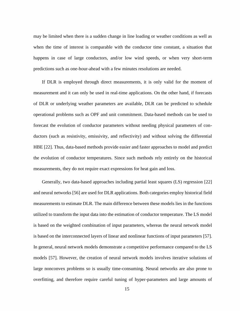
may be limited when there is a sudden change in line loading or weather conditions as well as
when the time of interest is comparable with the conductor time constant, a situation that
happens in case of large conductors, and/or low wind speeds, or when very short-term
predictions such as one-hour-ahead with a few minutes resolutions are needed.
If DLR is employed through direct measurements, it is only valid for the moment of
measurement and it can only be used in real-time applications. On the other hand, if forecasts
of DLR or underlying weather parameters are available, DLR can be predicted to schedule
operational problems such as OPF and unit commitment. Data-based methods can be used to
forecast the evolution of conductor parameters without needing physical parameters of con-
ductors (such as resistivity, emissivity, and reflectivity) and without solving the differential
HBE [22]. Thus, data-based methods provide easier and faster approaches to model and predict
the evolution of conductor temperatures. Since such methods rely entirely on the historical
measurements, they do not require exact expressions for heat gain and loss.
Generally, two data-based approaches including partial least squares (LS) regression [22]
and neural networks [56] are used for DLR applications. Both categories employ historical field
measurements to estimate DLR. The main difference between these models lies in the functions
utilized to transform the input data into the estimation of conductor temperature. The LS model
is based on the weighted combination of input parameters, whereas the neural network model
is based on the interconnected layers of linear and nonlinear functions of input parameters [57].
In general, neural network models demonstrate a competitive performance compared to the LS
models [57]. However, the creation of neural network models involves iterative solutions of
large nonconvex problems so is usually time-consuming. Neural networks are also prone to
overfitting, and therefore require careful tuning of hyper-parameters and large amounts of

16
training data. In contrast, regression models such as LS or quantile regression (QR) [58] are
obtained by solving convex optimization problems with a much smaller size. When applied to
estimate the conductor temperature, the performance of both models is very close with a
difference between mean square errors of less than one degree Celsius [56], making both models
acceptable. Therefore, the reliability and explicit parametrization of regression models, such as
LS, make them a viable alternative for DLR applications.
In view of the fact that a line with DLR is operated close to its thermal limits, the uncertainty
of forecasts may result in its capacity overestimation and therefore, it may increase the risk of
thermal overloading of the conductor. The uncertainty of DLR is investigated in [16] by a
scenario-based stochastic programming and by robust optimiztion in [17], [43]. However, these
methods are based on the steady-state model that neglects the thermal dynamics and may also
need a high computational burden that makes them unsuitable for short-term operational
problems, where fast methods are required.
In this context, data-based methods provide more practical approaches for DLR. The partial
LS model [22] that is based on field measurements is one such example. However, it fails to
address the forecast uncertainty and the risk of overloading. While the LS model can be used to
forecast conductor temperature or rating for the next time interval, it has not been applied in
operational problems. In particular, the method of [22] does not consider the case when the
conductor thermal dynamics introduce the dependence between the time intervals of the
operational problem. The forecast uncertainty can be addressed by the QR method as the
evolved version of the LS approach.

17
The QR method has been applied to forecast DLR in the recent literature, e.g., [42], [59].
In [42], a day-ahead QR model is proposed for steady-state DLR forecasting with the weather
parameter inputs. While [42] leads to accepta-ble results in day-ahead forecasting, its
performance depends on the careful tuning of some hyperparameters, such as the number of
regression trees as well as their depth and width. In addition, because its model is not explicitly
par-ametrized with respect to the conductor current, it cannot be directly embedded as a
constraint in power system ap-plications such as OPF. In [59], a QR-based model is proposed
to forecast the steady-state DLR for the hour ahead with measured weather parameters as inputs.
These works employ the steady-state model of the DLR mainly based on the CIGRE standard
[20]. Thus, they ignore the thermal dynamics of the conductor, which is a challenging feature
in the DLR.
Within the above context, main contributions of this part can be summarized as follows:
• Two data-based models of QR and superquantile regression (SQR) are proposed to
predict the conductor temperature evolution for DLR using time-lagged weather and conductor
current data. The SQR is applied as the first attempt to power system applications. The time-
lagged data enable us to model the conductor thermal dynamics when a high-resolution
prediction is performed with short time intervals comparable to the conductor thermal time
constant. Thus, the conductor capacity is more efficiently utilized in operational problems.
• A stochastic risk-averse framework is implemented to control uncertainties in estimating
the conductor temperature. It becomes especially valuable when a line is operated at its
boundary limits due to DLR, where any uncertainty can easily overload such a line. The
18
resulting models are data-based, fully parametric and easily extendable. Moreover, bilinear
terms are added to enhance the accuracy of the model.
• The proposed DLR model is translated into a closed modular constraint with coupling
among time slots to be incorporated into risk-based stochastic DLR applications. A multi-period
OPF is selected to evaluate the applicability of the proposed models and show its Pareto
optimality.
2.3 Underlying Concepts
2.3.1 Heat Balance Equation (HBE)
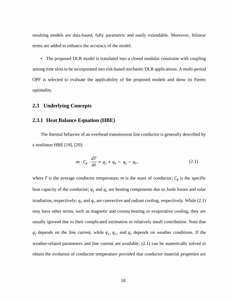
The thermal behavior of an overhead transmission line conductor is generally described by
a nonlinear HBE [19], [20]:
𝑚 ⋅ 𝐶𝑝 ⋅𝑑𝑇
𝑑𝑡= 𝑞𝐽 + 𝑞𝑠 − 𝑞𝑐 − 𝑞𝑟 , (2.1)
where 𝑇 is the average conductor temperature; 𝑚 is the mass of conductor; 𝐶𝑝 is the specific
heat capacity of the conductor; 𝑞𝐽 and 𝑞𝑠 are heating components due to Joule losses and solar
irradiation, respectively; 𝑞c and 𝑞r are convective and radiant cooling, respectively. While (2.1)
may have other terms, such as magnetic and corona heating or evaporative cooling, they are
usually ignored due to their complicated estimation or relatively small contribution. Note that
𝑞𝐽 depends on the line current, while 𝑞𝑠 , 𝑞𝑐 , and 𝑞𝑟 depends on weather conditions. If the
weather-related parameters and line current are available, (2.1) can be numerically solved to
obtain the evolution of conductor temperature provided that conductor material properties are
19
known. Alternatively, if the conductor temperature is set to its upper limit, the optimal value of
conductor current can be obtained from (2.1) for given weather parameters.
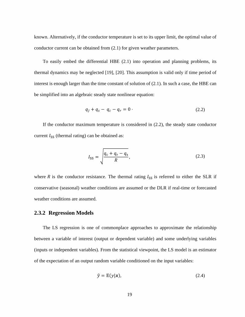
To easily embed the differential HBE (2.1) into operation and planning problems, its
thermal dynamics may be neglected [19], [20]. This assumption is valid only if time period of
interest is enough larger than the time constant of solution of (2.1). In such a case, the HBE can
be simplified into an algebraic steady state nonlinear equation:
𝑞𝐽 + 𝑞𝑠 − 𝑞𝑐 − 𝑞𝑟 = 0 ⋅ (2.2)
If the conductor maximum temperature is considered in (2.2), the steady state conductor
current 𝐼SS (thermal rating) can be obtained as:
𝐼SS = √𝑞c + 𝑞r − 𝑞s
𝑅, (2.3)
where 𝑅 is the conductor resistance. The thermal rating 𝐼SS is referred to either the SLR if
conservative (seasonal) weather conditions are assumed or the DLR if real-time or forecasted
weather conditions are assumed.
2.3.2 Regression Models
The LS regression is one of commonplace approaches to approximate the relationship
between a variable of interest (output or dependent variable) and some underlying variables
(inputs or independent variables). From the statistical viewpoint, the LS model is an estimator
of the expectation of an output random variable conditioned on the input variables:
�� = 𝔼(𝑦|𝒙), (2.4)

20
where 𝑦 is the output random variable; �� is its estimated mean; 𝒙 is the vector of input
variables. The linear form of the LS estimator is expressed as:
�� = 𝒙𝐓𝜷, (2.5)
where 𝜷 is the model parameter vector. The first element of 𝒙 equals to unity to create the “bias”
[57] (also known as “intercept” [58]) term. The bias term represents the base value of the output,
conditional on all 𝒙 inputs (excluding the first unity term) being zero. The introduction of the
bias term makes the regression model invariant to the affine scaling of the input and improves
the regression convergence [58]. In order to determine the parameter vector 𝜷, sum of squared
residuals between estimated ��𝑖 and observed 𝑦𝑖 is minimized for the known input-output pairs
(𝑦1, 𝒙1), … , (𝑦𝑛, 𝒙𝑛). Mathematically, the following optimization problem is solved for this
purpose:
𝜷 = argmin𝜷
∑(𝑦𝑖 − 𝒙𝑖T𝜷)
2𝑛
𝑖=1
, (2.6)
where 𝒙𝑖 and 𝑦𝑖 are the input vector and observed output, respectively, for data point 𝑖.
While the LS method estimates the conditional mean of the output variable, it does not
provide other distributional information. Instead, the distributional properties of a random
variable can be described by using quantile-based methods. Assuming that random variable 𝑦
is continuous, its 𝛼-quantile function can be defined as:
ℚα(𝑦) = min{𝑧|𝐹𝑦(𝑧) ≥ 𝛼} = 𝐹𝑦−1(𝛼), (2.7)
where 𝐹𝑦(⋅), 𝐹𝑦−1(⋅) are the cumulative distribution function (CDF) and its inverse function,
respectively, of 𝑦.

21
Similar to (2.5), the linear QR model is an estimator of the conditional 𝛼-quantile of 𝑦:
��α = ℚα(𝑦|𝒙) = 𝒙𝐓𝜷α, (2.8)
where ��α is the estimated 𝛼-quantile; 𝛼 ∈ [0,1] is the quantile level of the random variable; 𝜷α
is the model parameter vector.
Unlike the LS regression, QR can capture the whole conditional distribution of a random
variable [58]. In fact, QR can be used to estimate every conditional quantile including the
median. As a result, the risk associated with the tail outcomes can be quantified and controlled
in a systematic manner. In addition, compared with the LS regression, QR does not require the
assumption of the distribution of errors. Therefore, QR performs adequately in the presence of
outliers and is more successful when there is a weak relationship between the expected values
of variables. The QR parameter vector 𝜷α is obtained from a linear programming optimization
problem that can be efficiently solved by available solvers:
𝜷α = argmin𝜷α
∑ 𝜌𝛼(𝑦𝑖 − 𝒙𝑖T𝜷α)
𝑛
𝑖=1
, (2.9)
where 𝜌α(⋅) is the nominal absolute function described as:
𝜌𝛼(𝑢) = {𝛼𝑢 if 𝑢 ≥ 0
(𝛼 − 1)𝑢 if 𝑢 < 0 ⋅ (2.10)
While the QR is versatile and widely applicable in quantifying the risk, it can be further
extended to the SQR [60] in order to estimate the cumulative tail behavior of a random variable.
Unlike the QR that quantifies the risk only in terms of the probability of some undesirable event,

22
SQR reflects the magnitude of this event. This property is especially useful for applications,
where it is possible to address the consequences of undesirable events.
The 𝛼 -superquantile function of a continuous random variable 𝑦 is defined as its tail
expectation. In terms of the quantile function (2.7), the upper-tail 𝛼-superquantile function is
expressed as [60]:
ℚ𝛼(𝑦) = 𝔼(𝑦|𝑦 ≥ ℚ𝛼(𝑦)) =
1
1 − 𝛼∫ ℚ𝛽(𝑦)
1
𝛼
𝑑𝛽. (2.11)
Similar to other regressions, the linear SQR model is an estimator of the conditional 𝛼-
superquantile of 𝑦:
��α = ℚα(𝑦|𝒙) = 𝒙𝐓𝜷α, (2.12)
where ��α is the estimated upper-tail 𝛼-superquantile; α ∈ (0,1) is the superquantile level
of the random variable; 𝜷α is the model parameter vector. The lower-tail 𝛼 -superquantile
function ℚα(⋅) and its corresponding regression model can also be similarly defined. Since SQR
is evolved from QR, it inherits the advantage of determining its model parameter vector 𝜷α
through solving a linear programming problem. Further details of SQR can be found in [60].
The performance of LS, QR, and SQR is compared in Figure 2.1, where quadratic models
are fitted using data samples generated with the non-Gaussian noise assuming quantile and
superquantile levels at 0.95. The PSG toolbox is used to implement QR and SQR. As seen from
Figure 2.1, the LS model fits the expected value of the data well, but it does not provide
information about its distribution. To illustrate how different models capture the distributional
properties, the absolute error histograms are depicted in Figure 2.2. Note that positive errors in

23
this figure represent underestimation. As seen, the LS model underestimates the actual data,
whereas the QR model (with the selected 0.95 quantile) leads to about less than 5%
underestimation with a reduced peak. At the same time, the SQR further reduces the largest
errors by almost the half as well as the underestimation compared with the LS method.
Figure 2.1 Comparison of LS, QR, and SQR
Figure 2.2 Error histogram for a) LS, b) QR, and c) SQR methods

24
2.3.3 Risk-Averse Modeling of Uncertain Line Flows Using Chance
Constraints
Forecast weather parameters have some level of uncertainty that translates to the
uncertainty of the DLR forecasts and line flow constraints. By introducing a random variable 𝜉
corresponding to the random DLR capacity, a line flow constraint can be expressed as:
𝐻(𝜲) ≤ 𝜉, (2.13)
where 𝐻(𝜲) is the transmission line flow (power or current) as a function of decision vector 𝑿.
Since line flow constraint (2.13) cannot be directly incorporated into a programming-based
optimization problem, it is necessary to reformulate it. In the simplest case, the expected value
of 𝜉 can be used. However, as lines are usually operated at their thermal boundary rating in
DLR, errors in the DLR forecasts can lead to the violation of line flow constraints. Therefore,
it is desirable to control the risk of constraint violation.
Applying the chance-constrained approach, the probability of violation of the uncertain
constraint can be limited to the specified risk level [61]. The chance-constrained line flow can
be written as:
ℙ(𝐻(𝜲) ≤ 𝜉) ≥ 1 − 𝜖, (2.14)
where ℙ denotes probability; 0 < 𝜖 < 1 is the risk level. Assuming that the DLR capacity
random variable is continuous, the chance constraint (2.14) can be rewritten as:
ℙ(𝐻(𝜲) ≥ 𝜉) ≤ 𝜖, (2.15)
25
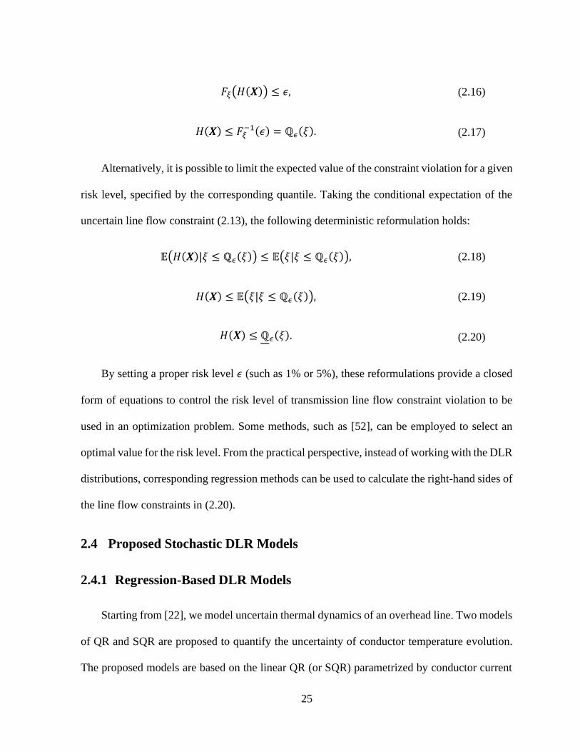
𝐹𝜉(𝐻(𝜲)) ≤ 𝜖, (2.16)
𝐻(𝜲) ≤ 𝐹𝜉−1(𝜖) = ℚ𝜖(𝜉). (2.17)
Alternatively, it is possible to limit the expected value of the constraint violation for a given
risk level, specified by the corresponding quantile. Taking the conditional expectation of the
uncertain line flow constraint (2.13), the following deterministic reformulation holds:
𝔼(𝐻(𝜲)|𝜉 ≤ ℚ𝜖(𝜉)) ≤ 𝔼(𝜉|𝜉 ≤ ℚ𝜖(𝜉)), (2.18)
𝐻(𝜲) ≤ 𝔼(𝜉|𝜉 ≤ ℚ𝜖(𝜉)), (2.19)
𝐻(𝜲) ≤ ℚ𝜖(𝜉). (2.20)
By setting a proper risk level 𝜖 (such as 1% or 5%), these reformulations provide a closed
form of equations to control the risk level of transmission line flow constraint violation to be
used in an optimization problem. Some methods, such as [52], can be employed to select an
optimal value for the risk level. From the practical perspective, instead of working with the DLR
distributions, corresponding regression methods can be used to calculate the right-hand sides of
the line flow constraints in (2.20).
2.4 Proposed Stochastic DLR Models
2.4.1 Regression-Based DLR Models
Starting from [22], we model uncertain thermal dynamics of an overhead line. Two models
of QR and SQR are proposed to quantify the uncertainty of conductor temperature evolution.
The proposed models are based on the linear QR (or SQR) parametrized by conductor current

26
and weather data forecasts as input vectors. These models forecast the 𝛼-quantile (or upper-tail
𝛼-superquantile) of conductor temperature ��𝑡𝛼 (or ��𝑡
𝛼) at time 𝑡 based on the input vectors at 𝑘
previous time intervals. The input vector is constructed from basic weather-related forecasts
including wind speed 𝑊𝑠, wind angle 𝑊𝑎 , ambient temperature 𝑇𝑎 , and solar radiation 𝑄𝑠 as
well as conductor current 𝐼𝑡. We include the conductor current magnitude and its square in the
input vector to represent the effects of both Joule heating and temperature-dependent resistance.
This set of input parameters is practically available from field measurement data collected for a
DLR conductor [8]. In particular, our input vector is expressed as:
𝑥𝑡 = [
[1, ℐ2, ℐ, 𝒲𝑠, 𝒲𝑎, 𝒯𝑎, 𝒬𝑠]𝑇
[𝒲𝑠𝒲𝑎 , 𝒲𝑠𝒯�� , 𝒲𝑠𝒬��, 𝒲𝑎𝒯�� , 𝒲𝑎𝒬��, 𝒯𝑎𝒬��]
𝑇
[𝒲𝑠𝒲𝑠 , 𝒲𝑎𝒲𝑎
, 𝒯𝑎𝒯��, 𝒬𝑠𝒬��]𝑇
] . (2.21)
In (2.21), ℐ2, ℐ, 𝒲𝑠, 𝒲𝑎, 𝒯𝑎, and 𝒬𝑠 are row vectors of squared current and its magnitude,
wind speed, wind angle, ambient temperature, and solar radiation, respectively, at 𝑘 previous
time periods as:
ℐ2 = [𝐼𝑡−12 , … , 𝐼𝑡−𝑘
2 ]
ℐ = [𝐼𝑡−1, … , 𝐼𝑡−𝑘]
𝒲𝑠 = [𝑊𝑠,𝑡−1, … , 𝑊𝑠,𝑡−𝑘]
𝒲𝑎 = [𝑊𝑎,𝑡−1, … , 𝑊𝑎,𝑡−𝑘]
𝒯𝑎 = [𝑇𝑎,𝑡−1, … , 𝑇𝑎,𝑡−𝑘]
𝒬𝑠 = [𝑄𝑠,𝑡−1, … , 𝑄𝑠,𝑡−𝑘] ⋅
(2.22)

27
Bilinear terms are also included in (2.21). For instance, 𝒲𝑠𝒲𝑎 =
[𝑊𝑠,𝑡−1𝑊𝑎,𝑡−1, … , 𝑊𝑠,𝑡−𝑘𝑊𝑎,𝑡−𝑘] refers to the product of wind speed and angle. We have
embedded bilinear terms in (2.21) to better capture the possible interdependence between input
parameters. These bilinear terms enhance the impact of extreme parameters on estimation by
more efficiently modeling correlations among these parameters. For example, correlations can
happen when wind speeds are lower during overnight hours (when the temperature is lower), or
when there is a correlation between solar irradiation and ambient temperature.
The procedure for the creation of data-based models follows similar steps. As an example,
the SQR model for a prescribed risk level 𝛼 is obtained by solving the optimization problem
formulated in [60]. Input vectors 𝒙𝒊 in (2.21) are constructed from historical forecasts of
weather parameters and conductor current and regressed against the historical measurements of
conductor temperature 𝑦𝑖 = 𝑇𝑖 as the output. Then, to estimate the conductor temperature
superquantile at time 𝑡 , input vector (2.21) is constructed based on the relevant data and
substituted into (2.12) to calculate the forecasted 𝛼-superquantile of conductor temperature. The
resulting SQR model has the following closed form:
��𝑡𝛼 = 𝛽𝛼
0 + ∑ 𝛽𝛼
ℐ𝑡−𝑗2
𝐼𝑡−𝑗2
𝑘
𝑗=1
+ ∑ 𝛽𝛼
ℐ𝑡−𝑗𝐼𝑡−𝑗
𝑘
𝑗=1
+ ∑ 𝑊𝐹𝐶𝑡−𝑗
𝑘
𝑗=1
, (2.23)
where ��𝑡α is the estimated 𝛼-superquantile conductor temperature at time 𝑡; 𝛽𝛼
0, 𝛽𝛼
ℐ𝑡−𝑗2
and 𝛽𝛼
ℐ𝑡−𝑗
are the parameters corresponding with entry 1 (the bias term), vectors ℐ2 and ℐ in (2.21),
respectively. The last term in (2.23) includes remaining parts associated with weather-related
forecasted parameters 𝒲𝑠, 𝒲𝑎, 𝒯𝑎, and 𝒬𝑠 from time period 𝑡 − 𝑘 to 𝑡 − 1.

28
Due to the modular structure of the proposed models (2.21)–(2.23), it is straightforward to
add other features such as ones related to snowy or rainy weather conditions by including their
corresponding input variables. Moreover, the data-driven approaches, when compared with
analytical ones, may need a limited amount of conductor parameters, and they have the
capability to recreate their models by the information existent in the streams of time-series data.
They also allow to adjust and control the thermal overload risk as described in the next
subsection.
2.4.2 Stochastic DLR Models as Line Flow Constraints
While the reformulations of uncertain line flow constraints in (2.17) and (2.20) for the QR
and SQR models can be used with the steady-state DLR, they cannot be applied in the models
with thermal dynamics due to time coupling and non-static nature of conductor temperature.
Eq. (2.23) gives a closed-form relation for the SQR estimation of the 𝛼-superquantile conductor
temperature from time-series data of weather parameters and conductor current at 𝑘 previous
time slots. Then, by setting the 𝛼-superquantile of the conductor temperature to its maximum
permitted value ��𝑡α = 𝑇max in (2.23) and relaxing the equality into inequality, it is possible to
limit the risk of conductor overheating. Then, due to its parametric form, (2.23) can be used to
establish a relation among weather parameters and conductor current (lagged time periods 𝑡 −
𝑘 to 𝑡 − 1):
𝛽𝛼0 + ∑ 𝛽𝛼
ℐ𝑡−𝑗2
𝐼𝑡−𝑗2
𝑘
𝑗=1
+ ∑ 𝛽𝛼
ℐ𝑡−𝑗𝐼𝑡−𝑗
𝑘
𝑗=1
+ ∑ 𝑊𝐹𝐶𝑡−𝑗
𝑘
𝑗=1
≤ 𝑇max ⋅ (2.24)

29
Eq. (2.24) can be used as a quadratic constraint in different optimization problems, such as
multi-period OPFs, for the data-based models. Since these DLR models are included for each
time period, time coupling of multi-period applications are observed.
Considering 𝑘 = 1 in (2.24), it is possible to get a simpler closed expression for the
conductor current at each time period as a conventional capacity constraint:
where 𝐼𝑡−1𝑚𝑎𝑥, representing the maximum value of 𝐼𝑡−1, is expressed as a function of weather
parameters 𝑊𝐹𝐶𝑡−1.
2.4.3 Overall Proposed Algorithm for DLR
The proposed algorithm is presented in Figure 2.3. First, the data-driven DLR model is
created based on the historical data. After specifying the risk level and number of time lags, the
model parameters are estimated as 𝛽 values used in equation (2.24). In the next step as the
operational scheduling and using the DLR model, OPFs are constructed and solved for each
time interval of the evaluation period. Because weather parameters predicted for the scheduling
interval are also used in the OPFs, their solution including the conductor current may have some
uncertainty due to forecast errors. Finally, using the conductor current and actual realizations of
weather parameters, the conductor temperature is calculated by means of the heat-balance
equation (2.1). After solving the OPFs for all time intervals, the actual risk is calculated as the
ratio of the number of time intervals with excessive temperature to the total number of time
intervals.
𝐼𝑡−1𝑚𝑎𝑥 =
−𝛽𝛼ℐ𝑡−1
2𝛽𝛼ℐ𝑡−1
2 +√(𝛽𝛼
ℐ𝑡−1)2
− 4𝛽𝛼ℐ𝑡−1
2
(𝛽α0 + 𝑊𝐹𝐶𝑡−1 − 𝑇max)
2𝛽𝛼ℐ𝑡−1
2 , (2.25)

30
Figure 2.3 Proposed algorithm for DLR
2.5 Application of the Proposed DLR Model to OPF
The obtained time-coupled conductor current constraint (2.24) can be incorporated into
different power system applications including OPF. We here consider a standard multi-period
AC OPF to demonstrate the underlying ideas as formulated below.
Estimate model parameters β
DLR model creation
Compose the OPF model with DLR constraints
Solve OPF
Operational scheduling with DLR
Input historical data 1) conductor temperature and current measured, 2) weather data including wind speed, wind angle,
ambient temperature, and solar radiation
Input parameters: risk level, number of time lags (k)
Input weather forecasts for the scheduling interval ahead
Conductor temperature
Actual realizations of weather parameters
Heat-balance equation
Conductor temperature
Conductor current
Rep
eat
thes
e tw
o s
teps
for
ever
y O
PF
to
calc
ula
te t
he
actu
al r
isk
31
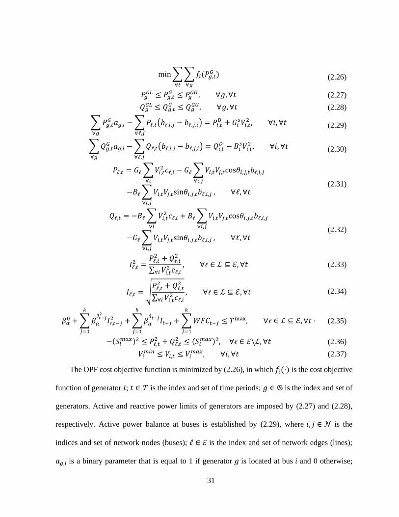
The OPF cost objective function is minimized by (2.26), in which 𝑓𝑖(⋅) is the cost objective
function of generator 𝑖; 𝑡 ∈ 𝒯 is the index and set of time periods; 𝑔 ∈ 𝔊 is the index and set of
generators. Active and reactive power limits of generators are imposed by (2.27) and (2.28),
respectively. Active power balance at buses is established by (2.29), where 𝑖, 𝑗 ∈ 𝒩 is the
indices and set of network nodes (buses); ℓ ∈ ℰ is the index and set of network edges (lines);
𝑎𝑔,𝑖 is a binary parameter that is equal to 1 if generator 𝑔 is located at bus 𝑖 and 0 otherwise;
min ∑ ∑ 𝑓𝑖(𝑃𝑔,𝑡𝐺 )
∀𝑔∀𝑡
(2.26)
𝑃𝑔𝐺𝐿 ≤ 𝑃𝑔,𝑡
𝐺 ≤ 𝑃𝑔𝐺𝑈 , ∀𝑔, ∀𝑡 (2.27)
𝑄𝑔𝐺𝐿 ≤ 𝑄𝑔,𝑡
𝐺 ≤ 𝑄𝑔𝐺𝑈, ∀𝑔, ∀𝑡 (2.28)
∑ 𝑃𝑔,𝑡𝐺 𝑎𝑔,𝑖
∀𝑔
− ∑ 𝑃ℓ,𝑡(𝑏ℓ,𝑖,𝑗 − 𝑏ℓ,𝑗,𝑖)
∀ℓ,𝑗
= 𝑃𝑖,𝑡𝐷 + 𝐺𝑖
𝑠𝑉𝑖,𝑡2 , ∀𝑖, ∀𝑡 (2.29)
∑ 𝑄𝑔,𝑡𝐺 𝑎𝑔,𝑖
∀𝑔
− ∑ 𝑄ℓ,𝑡(𝑏ℓ,𝑖,𝑗 − 𝑏ℓ,𝑗,𝑖)
∀ℓ,𝑗
= 𝑄𝑖,𝑡𝐷 − 𝐵𝑖
𝑠𝑉𝑖,𝑡2 , ∀𝑖, ∀𝑡 (2.30)
𝑃ℓ,𝑡 = 𝐺ℓ ∑ 𝑉𝑖,𝑡2 𝑐ℓ,𝑖
∀𝑖
− 𝐺ℓ ∑ 𝑉𝑖,𝑡𝑉𝑗,𝑡cos𝜃𝑖,𝑗,𝑡𝑏ℓ,𝑖,𝑗
∀𝑖,𝑗
−𝐵ℓ ∑ 𝑉𝑖,𝑡𝑉𝑗,𝑡sin𝜃𝑖,𝑗,𝑡𝑏ℓ,𝑖,𝑗
∀𝑖,𝑗
, ∀ℓ, ∀𝑡 (2.31)
𝑄ℓ,𝑡 = −𝐵ℓ ∑ 𝑉𝑖,𝑡2 𝑐ℓ,𝑖
∀𝑖
+ 𝐵ℓ ∑ 𝑉𝑖,𝑡𝑉𝑗,𝑡cos𝜃𝑖,𝑗,𝑡𝑏ℓ,𝑖,𝑗
∀𝑖,𝑗
−𝐺ℓ ∑ 𝑉𝑖,𝑡𝑉𝑗,𝑡sin𝜃𝑖,𝑗,𝑡𝑏ℓ,𝑖,𝑗
∀𝑖,𝑗
, ∀ℓ, ∀𝑡 (2.32)
𝐼ℓ,𝑡2 =
𝑃ℓ,𝑡2 + 𝑄ℓ,𝑡
2
∑ 𝑉𝑖,𝑡2 𝑐ℓ,𝑖∀𝑖
, ∀ℓ ∈ ℒ ⊆ ℰ, ∀𝑡 (2.33)
𝐼ℓ,𝑡 = √𝑃ℓ,𝑡
2 + 𝑄ℓ,𝑡2
∑ 𝑉𝑖,𝑡2 𝑐ℓ,𝑖∀𝑖
, ∀ℓ ∈ ℒ ⊆ ℰ, ∀𝑡 (2.34)
𝛽𝛼0 + ∑ 𝛽𝛼
ℐ𝑡−𝑗2
𝐼ℓ,𝑡−𝑗2
𝑘
𝑗=1
+ ∑ 𝛽𝛼
ℐ𝑡−𝑗𝐼𝑡−𝑗
𝑘
𝑗=1
+ ∑ 𝑊𝐹𝐶𝑡−𝑗
𝑘
𝑗=1
≤ 𝑇max, ∀ℓ ∈ ℒ ⊆ ℰ, ∀𝑡 ⋅ (2.35)
−(𝑆𝑙𝑚𝑎𝑥)2 ≤ 𝑃ℓ,𝑡
2 + 𝑄ℓ,𝑡2 ≤ (𝑆𝑙
𝑚𝑎𝑥)2, ∀ℓ ∈ ℰ\ℒ, ∀𝑡 (2.36)
𝑉𝑖𝑚𝑖𝑛 ≤ 𝑉𝑖,𝑡 ≤ 𝑉𝑖
𝑚𝑎𝑥, ∀𝑖, ∀𝑡 (2.37)

32
𝑃ℓ,𝑡 is the active power flow of line ℓ at time period 𝑡; 𝑏ℓ,𝑖,𝑗 is a binary parameter that equals to
1 if line ℓ connects buses 𝑖 and 𝑗 and 0 otherwise; 𝑃𝑖,𝑡𝐷 is the active power demand of bus 𝑖 at
time period 𝑡; 𝐺𝑖𝑠 is the shunt conductance at bus 𝑖; 𝑉𝑖,𝑡 is the voltage magnitude of bus 𝑖 at time
period 𝑡. Similarly, reactive power balance at buses is imposed by (2.30), where 𝐵𝑖𝑠 is the shunt
susceptance at bus 𝑖. Active power flow of lines is given by (2.31), in which 𝐺ℓ and 𝐵ℓ represent
the conductance and susceptance of line ℓ, respectively; 𝑐ℓ,𝑖 is a binary parameter that equals to
1 if line ℓ is connected to bus 𝑖 and 0 otherwise; 𝜃𝑖,𝑗,𝑡 = 𝜃𝑖,𝑡 − 𝜃𝑗,𝑡 ; 𝑉𝑖,𝑡∠𝜃𝑖,𝑡 is the voltage
phasor of bus 𝑖 voltage at time period 𝑡. Similarly, (2.32) gives reactive power flow of lines.
The square of the conductor current of DLR-controlled lines ℓ ∈ ℒ ⊆ ℰ at time period 𝑡 and its
current value are given by (2.33) and (2.34). Similar to (2.24), the conductor temperature of
DLR-controlled line ℓ is constrained by (2.35) in terms of 𝛼-quantile or the 𝛼-superquantile for
QR or SQR, respectively. It is noted that since (2.35) incorporates the risk-based stochastic DLR
into the OPF in a modular manner, it can also be easily incorporated in other applications. The
MVA power of non-DLR lines and voltage magnitude of buses are constrained by (2.36) and
(2.37), respectively.
2.6 Case Study and Numerical Results
The proposed method is examined on the updated RTS network [62] assuming one-hour-
ahead multi-period OPF with a five-minute time resolution. The line between buses 15–21 with
the length 60 km is chosen to be monitored for DLR. Its conductor is considered “Falcon” 72/7
with type of aluminum conductor steel-reinforced (ACSR) with the maximum temperature
rating set at 80 C. The SLR current of the conductor is assumed to be 1269 A calculated at the
conditions of ambient temperature 35 C, perpendicular wind speed 0.6 m/s, and solar radiation
33
900 W/m2. The risk level for risk-averse models is set at 5%. Other non-DLR lines of the test
system are limited with their MVA rating, and the voltage magnitude of buses is confined into
the range [0.95, 1.05] pu.
For historical time-series data, we use the hourly weather data available from the
“Assiniboia Airport” weather station in Saskatchewan, Canada. We interpolate these data to
have a dataset with a 5-minute resolution, which is short enough to capture dynamic variations
of weather conditions. We use the data from June and July 2019 to estimate the DLR models
and data from August 2019 to evaluate and validate the proposed models.
To evaluate and compare the proposed method in different situations, the following models
are considered:
• SLR: The static line rating model.
• LS: The LS based model [22] having the structure of (2.24) with 𝑘 = 3.
• CC: The standard chance-constrained based on the steady-state model (2.3).
• QR: The proposed QR DLR model (2.24) with 𝑘 = 1, 2, 3 (referred to QR1, QR2, and QR3,
respectively).
• SQR: The proposed SQR DLR model (2.24) with 𝑘 = 1, 2, 3 (referred to SQR1, SQR2, and
SQR3, respectively).
The SLR model provides the static rating of the line using conservative weather
assumptions. The LS forecast model uses three time lags (𝑘 = 3) of historical data. Model CC
reveals the effect of imposing chance constraints on the steady state DLR forecast. By
comparing SLR and CC models, it is possible to find out the overall effect of chance-constrained

34
DLR on its conventional implementation. Models SLR and CC do not consider the conductor
time evolution. The QR and SQR models are implemented with three different values of time
lags 𝑘 to reveal the effect of time lags in (2.24) on prediction. All above-mentioned models are
built using data from June and July 2019 and then, forecast data from August 2019 are used in
OPFs based on the created models; next, models are validated using actual data from August
2019.
It is noted that the predicted values of weather parameters, which are labeled 𝑊𝐹𝐶 in
(2.24), are used in the forecast of all examined models. Because these predicted weather
parameters have some forecast errors, the actual conductor temperature may violate its
allowable limit when calculated with the actual realizations of weather parameters and the
scheduled conductor current. One result is a probability of excess conductor temperature
conditioned on the uncertainty of weather parameters. Each risk-averse model (i.e., CC, QR1,
QR2, QR3, SQR1, SQR2, and SQR3) manages this risk with its own strategy.
Results of the examined models are presented in Table 2.1 with average performance
indices over the evaluation period, which includes August 2019 with 31 days (with 744 hourly
OPFs). In column 2, the amount of transferred energy through the DLR conductor is reported.
In column 3, the average excess temperature is reported for hours that violate the maximum 80
C conductor temperature limit when actual realizations of weather data are applied. In column
4, the actual risk is calculated as the ratio of the number of time intervals with conductor
temperature violation to the total number of time intervals. If the OPF cost for the SLR method
is considered 100%, the cost of other models in Table 2.1 have similar values ranging from
95.13% to 95.84%. Since the cost mainly depends on other network parameters, such as

35
generator cost functions and network congestion, it may not present a relationship with risk-
based quantities.
Table 2.1 Results of Examined Modes
Model Average energy transferred (MWh) Average excess temperature (C) Actual risk (%)
SLR 302.8 80.2 0.02
LS 407.7 90.5 6.29
CC 390.9 85.1 0.81
QR1 397.6 85.3 1.44
QR2 398.9 84.4 1.32
QR3 400.9 84.7 1.85
SQR1 391.3 84.9 0.73
SQR2 393.7 83.9 0.87
SQR3 394.3 84.2 1.24
As seen from Table 2.1, all risk-averse and SLR models manage to reduce the actual risk
within the preset value 5%. However, because the LS model fails to consider the risk, it results
in a solution with the highest actual risk 6.29%. Although the LS model leads to a higher level
of transferred energy (407.7 MWh), it has the worst average excess conductor temperature (90.5
C) and leads to an insecure solution. In contrast, although the SLR model has the lowest risk
and excess temperature, its transferred energy (302.8 MWh) is too low implying a solution that
is too conservative and not cost-effective. The CC model, which is risk-averse but without
coupling between time periods, leads to a transferred energy of 390.9 MWh (higher than the
SLR model) as well as an acceptable risk (0.81%) and excess temperature (85.1 C). The QR2
model offers a slightly higher transferred energy (398.9 MWh) than the QR1 model even with
lower excess temperature and risk. The QR3 model offers a slightly higher transferred energy
than the QR2 model with a similar excess temperature, but with a higher risk (1.85%). Thus,
among the QR1, QR2, and QR3 models, the QR2 solution may represent a preferred

36
compromise in terms of the three parameters in Table 2.1. SQR models are generally more risk-
averse than QR models.
Figure 2.4 Solutions by the examined models and Pareto-optimal front
It is worthwhile to note that the risk and benefit are two competitive targets; by optimizing
one of them, the other one may be deteriorated. Since the goal of DLR is to increase energy
transfer capability of an overhead line, it is selected here as the desired benefit objective. On
the other hand, given that the assigned risk level of 5% holds for all risk-averse methods in
Table 2.1, the average excess temperature is selected here as the risk objective. This is motivated
by the fact that small overheating can be smoothed out because of the conductor thermal inertia,
and it is better handled in real-time operation when actual measurements are available. For these
two metrics, the Pareto front is plotted in Figure 2.4 using the obtained solutions. This Pareto
front helps the power system operator choose one of solutions to be implemented. Solutions by
the SLR and LS are able to optimize only one of objective functions and then, the other one is

37
deteriorated. As seen from Figure 2.4, the QR2 solution provides the most acceptable tradeoff
between the average excess temperature and transferred energy. Therefore, the QR2 solution
may be the preferred one. In next stages, solutions by SQR2 and QR3 may make acceptable
tradeoff between the two competing objective functions. Solutions by SQR1, CC, and QR1 fail
to make acceptable tradeoffs between the two objective functions.
In order to perform a more detailed analysis, the conductor temperature, current, and
transferred power in selected hour 86 are plotted in Figure 2.5 for models QR2 and SQR2 (as
the preferred ones) and CC (as an outlier) with a five-minute resolution. As seen from Figure
2.5 (a), the selected hour encounters heavily loaded conditions and extreme weather parameters,
and the conductor temperature reaches values above its allowable 80 C limit when the actual
realizations of weather parameters are applied. The maximum experienced conductor
temperature for models CC, QR2, and SQR2 in Figure 2.5 (a) is 89.2, 85.8, and 85.3 C,
respectively. This figure shows that the examined models perform similarly when the loading
level is low (early times in the horizontal axis); that is, all models are able to estimate a sufficient
transmission margin. However, they perform differently in higher loading times (starting from
around 𝑡 = 25 min in Figure 2.5 (b)-(c)). One interesting difference in this figure is the
preemptive reduction of conductor temperatures by the QR2 and SQR2 models. When the
current or power in Figure 2.5 (b)-(c) starts to increase from around 𝑡 = 25 min, the conductor
temperature is affected after some delays due to the thermal inertia of the conductor, with the
conductor temperature reaching its peak later at around 𝑡 = 45 min in Figure 2.5 (a). Because
the QR2 and SQR2 models consider time coupling, here they are able to mitigate the excessive
temperature; this is not the case for the CC model that does not consider the time coupling.
Consequently, the CC model results in the conductor facing the highest temperatures for longer

38
periods, whereas the QR2 and SQR2 models lead to lower maximum temperatures. This
analysis is only for the selected hour; the average performance of the examined models over the
entire evaluation period is presented in Table 2.1.
Figure 2.5 Variation of conductor parameters in the selected hour with actual realizations
of weather parameters: (a) temperature, (b) current, and (c) transmitted power
In order to evaluate the effect of bilinear terms of input vector on performance metrics, the
SQR2 method is selected to be implemented with/without bilinear terms. Results are presented

39
in Table 2.2. As seen in this table, while the introduction of bilinear terms has a minor impact
on the average energy transfer, it significantly affects the ability of the model to address the risk
and the temperature of the overloading. The two last metrics in Table 2.2 describe the statistical
distribution of forecast residuals caused by the weather forecast error. As seen, predictions with
considering the bilinear terms results in a better forecast with lower standard deviation and mean
absolute deviation implying more robust results.
Table 2.2 Effect of Bilinear Terms on the Solution
Metric SQR2 without bilinear terms SQR2 with bilinear terms
Average energy transmitted (MWh) 393.0 393.7
Average excess temperature (C) 85.5 83.9
Actual risk (%) 3.12 0.87
Standard deviation (C) 9.7 8.6
Mean absolute deviation (C) 7.0 6.4
The forecast error of weather parameters impacts DLR performance. The standard
deviation of the forecast error can be employed as an index, where ideally a zero standard
deviation implies no forecast error, and a higher standard deviation indicates a lower forecast
accuracy. The impact of forecast error standard deviation is presented in Table 2.3 for wind
speed and ambient temperature, as the most influential weather parameters on the DLR, solved
by SQR1. For each time interval in the evaluation period (August 2019), the weather parameter
is forecast and then, its forecast error is calculated using its actual realization. Afterwards, the
standard deviation of the forecast error time series is calculated as reported in Table 2.3 for each
dataset. New datasets are generated using the variance scaling method, in which the error time
series is scaled by a coefficient, and then, the forecast time series is estimated in a backward
manner as a new dataset. Finally, after creating the DLR model (Figure 2.3) for each dataset,

40
the conductor rating is calculated using (2.25) as reported in Table 2.3. As seen in this table,
when the standard deviation of forecast errors of weather parameters increases, the conductor
rating decreases. It implies that a more accurate forecast model schedules the conductor capacity
more effectively.
Table 2.3 Impact of Weather Forecasting Errors on the Conductor Rating
Standard deviation of wind
speed forecast error (m/s)
Standard deviation of ambient
temperature forecast error (C)
Average estimated
conductor rating (kA)
1.23 1.56 1.91
1.51 1.92 1.85
1.74 2.21 1.81
1.94 2.47 1.78
2.13 2.71 1.75
2.7 Conclusions
In this work, two data-based models including QR and SQR are presented to estimate
dynamic line rating values considering thermal evolution of conductors. Uncertainty in weather-
related forecast values are modeled by a risk-averse method to prevent overloading risk of
conductors. The proposed method is finally converted to a closed relation constraint that is
appropriate for optimization problems such as OPF. From our case studies, we have found that
1) the proposed methods result in Pareto-optimal solutions making a tradeoff between conductor
transmitted energy and excess temperature when compared with other existing SLR, LS, and
CC methods, 2) the QR method with two time lags provides 31.7% more transmitted energy
than the SLR solution, 3) compared with the CC method, QR and SQR solutions with two time
lags offer higher values of conductor energy transfer capacity and lower excessive conductor
temperature when the actual realizations of weather parameters are applied.

41
3 A Framework for Power System Operational Planning under
Uncertainty Using Coherent Risk Measures
3.1 Abstract
With the increasing integration of renewable energy sources (RESs) and the
implementation of dynamic line rating (DLR), the accompanying uncertainties in power
systems require intensive management to ensure reliable and secure operational planning.
However, while numerous approaches and methods in the literature deal with uncertainty, they
have not been analyzed axiomatically. This work presents an analysis of risk in power system
operation using coherent risk measures, elaborating on the origin of risk and the mechanisms of
its management in the presence of various sources of uncertainty. To illustrate the practicality
and benefits of coherent risk measures, a risk-averse asymmetry robust unit commitment (UC)
model is established. It is based on coherent reformulations of the uncertain reserve and line
flow constraints and is formulated in the form of a compact computationally efficient mixed-
integer second-order conic program (SOCP). The overall performance of the proposed
framework is verified using the updated 2019 IEEE Reliability Test System over a year-long
period.
3.2 Nomenclature
• Problem Parameters:
𝓖 Set of conventional generators.
𝓓 Set of loads.
𝓡 Set of renewable energy sources.

42
𝓛𝐃 Set of lines with dynamic line rating.
𝓛𝐒 Set of lines without dynamic line rating.
𝓣 Set of time intervals.
𝜋𝑙,𝑖 Power transfer distribution factor of line 𝑙 for the origin bus 𝑖.
𝑃𝑙max Maximum capacity of line 𝑙.
𝑃𝑔max/𝑃𝑔
min Maximum/minimum output of generator 𝑔.
𝑅𝑔up/𝑅𝑔
𝑑own Up/down ramp capability of generator 𝑔.
𝜏𝑔on/𝜏𝑔
off Minimum online/offline time of generator 𝑔.
𝑓𝑔(⋅) Cost function of generator 𝑔.
𝑐𝑔su/𝑐𝑔
sd Start-up/shut-down cost of generator 𝑔.
𝑃𝑑,𝑡 Demand of load 𝑑 at time 𝑡.
𝑃𝑟max Maximum output (capacity) of renewable energy source (RES) r.
• Conventional Optimization Variables:
𝑃𝑔,𝑡 Output of generator 𝑔 at time 𝑡.
𝑢𝑔,𝑡 On/off status of generator 𝑔 at time 𝑡.
𝑣𝑔,𝑡 Start-up status of generator 𝑔 at time 𝑡.
𝑤𝑔,𝑡 Shut-down status of generator 𝑔 at time 𝑡.
• Robust Framework Parameters and Variables:
𝑃𝑟,𝑡 Scheduling variable of RES 𝑟 at time 𝑡.
��𝑟,𝑡 Forecast random variable of RES 𝑟 at time 𝑡.
𝑃𝑟,𝑡0 Nominal value of forecast random variable of RES 𝑟 at time 𝑡.
𝑝𝑟,𝑡/𝑞𝑟,𝑡 Forward/backward deviation of forecast random variable of RES 𝑟 at time 𝑡.
𝑃𝑟,𝑡/𝑃𝑟,𝑡 Upper/lower bound of the zero mean forecast random variable of RES 𝑟 at time 𝑡.
��𝑙,𝑡 Forecast random variable of dynamic line rating (DLR) for line 𝑙 at time 𝑡.
𝑃𝑙,𝑡0 Nominal value of forecast random variable of DLR for line 𝑙 at time 𝑡.

43
𝑝𝑙,𝑡/𝑞𝑙,𝑡 Forward/backward deviation of forecast random variable of DLR for line 𝑙 at time
𝑡.
𝑃𝑙,𝑡/𝑃𝑙,𝑡 Upper/lower bound of the support of the zero mean forecast random variable of DLR
for line 𝑙 at time 𝑡.
Ω Uncertainty budget parameter.
𝜖 Probability of constraint violation.
𝒚 Vector of robust counterpart auxiliary variables.
𝒓/𝒔 Vector of upper/lower bound auxiliary variables.
3.3 Introduction
With the recent and ongoing changes in modern power systems, the uncertainty therein is
becoming more impactful, widespread, and diverse, effectively itself constituting an inherent
property. To implement energy sustainability and emission reductions, a considerable amount
of current conventional generation is being replaced with renewable energy sources (RESs),
primarily in the form of wind and solar power. While RESs have numerous benefits, their output
is highly variable, which introduces forecast uncertainty and can result in the violation of
operating constraints. Furthermore, the successful integration of large numbers of RESs also
relies on the transfer capacity of the transmission network, which is potentially congested.
Conventionally, system operators determine the capacity of thermally limited transmission lines
based on their static line rating (SLR), which assumes conservative weather conditions.
Alternatively, the dynamic line rating (DLR) calculated based on relevant weather conditions
provides accurate estimations of transmission line capacity [19], allowing the system operator
to more efficiently utilize existing infrastructure. The DLR can lead to a decrease in the number
and severity of transmission congestions, decrease in operating costs, and increase in renewable
energy utilization [9]. However, direct application of DLR forecasts may also lead to an

44
overestimation of the capacity and result in overloading due to the inherent uncertainty [17],
[43]. Thus, the inclusion of the DLR in operational planning problems should consider not only
its benefits but also the related risks.
As power systems are undergoing such significant changes, forecast uncertainty becomes
a systemic issue affecting power system operational planning problems. One way to address the
uncertainty is by using the stochastic programming approach, such as two-stage stochastic unit
commitment (UC) [63], [64] that aims to minimize first stage commitment costs and the
expected costs due to the second stage realizations of uncertain parameters. While stochastic
programming is intuitive and easily extendable, it suffers from prohibitively high
dimensionality, necessitating decomposition algorithms, and cannot provide performance
guarantees. Alternatively, the worst-case costs during the second stage can be minimized with
respect to some set of uncertainty parameters. An example of such an approach is two-stage
robust UC [65], [66], which often results in highly secure but significantly less economical
solutions. Recently, a subject of intense research has been distributionally robust optimization,
which assumes that the actual distribution of the uncertain parameters is not known but belongs
to some family of distributions. A distributional family is commonly defined using the
information of its moments [67], by some distance function with respect to a data sample [68],
[69], or a combination of both [43]. Risk-based approaches provide another way of dealing with
uncertainty by defining a function between the undesirable outcome and underlying uncertain
parameters, for example, chance-constrained UC [70], mean-variance formulation of UC [71],
as well as models based on coherent risk measures, as discussed next.
Ultimately, all existing approaches can be understood as dealing with the consequences of
the realizations of uncertain parameters, labelled as “risk” in a broader sense of the term [72].

45
The framework of coherent risk measures presented in [72] and [73] provides an axiomatic
foundation that enables qualitative analysis of risk. Moreover, particular coherent risk measures
provide quantitative definitions of risk and allow flexible management of risk in a tractable and
computationally efficient way [74], [75]. Originally developed for the needs of the financial
sector, the coherent risk measures framework is suitable for any application concerned with risk
evaluation and management. Thus, one of the most widely used coherent risk measures,
conditional value-at-risk (CVaR) [73], has been successfully applied in various power systems
problems. CVaR has been used in the electricity market setting for distributed market clearing
in [76], risk-averse decision making for demand-side resource aggregators in [77], and wind
power producers in [78]. CVaR has also been integrated into operational planning problems.
For example, a two-stage stochastic UC formulation is proposed in [79] for isolated power
systems, a multi-stage UC model for smart grids is developed in [80], a security-constrained
UC model is proposed in [81], and the decomposition approaches are investigated in [82].
CVaR is a reasonable choice of a coherent risk measure in most applications, but its
performance depends on the sample size and sampling method. As a result, ensuring
performance guarantees can make the problem size prohibitively large due to the required
addition of extra variables and constraints for each sample. This situation is particularly relevant
in the presence of discrete variables and multiple uncertain constraints, as is the case of UC.
Moreover, the properties of coherent risk measures are often underutilized due to the way that
uncertainty is implemented. That is, most of the existing formulations consider the RES
forecasts as passive sources of uncertainty, neglecting the option of managing risk by actively
adjusting the expected power from RESs during the operational planning. Most importantly,
from the axiomatic perspective of risk measures, the phenomenon of risk associated with power

46
system operational planning under uncertainty has not been studied and analyzed in a systematic
and unified way.
In this work, the coherent risk measures framework is applied to analyze the risk of power
system operational planning under uncertainty, resulting in the first introduction of a systematic
treatment of risk. First, coherent reformulations of uncertain constraints are presented, with
RESs formulated as schedulable and multiplicative sources of uncertainty. Second, the
interactions between random and deterministic factors and their effects on the risk of constraint
violations are analyzed. The relationship between coherent risk measures and the reduction of
risk is presented. Third, a risk-averse robust UC model implementing the coherent
reformulations of the uncertain power reserve and line flow constraints is developed. The
reformulation is based on an asymmetric uncertainty set with a compact formulation and
provides guarantees of constraint violation probability. Lastly, the ability of the proposed
framework to efficiently manage the risks caused by different sources of uncertainty in a unified
way is demonstrated by comprehensive year-long case studies.
The main contributions of this work are summarized as follows:
1) Analysis and interpretation of risk in power system operational planning are performed for
the first time using the coherent risk measures framework. The relationships between
various sources of uncertainty and risk are explained and quantified.
2) Reformulations of uncertain power system constraints are developed in a fully coherent
way. Also, a new method of modelling uncertain RESs with adjustable power references is
proposed for flexible risk management in operational planning problems.

47
3) A risk-averse robust UC model is established with coherent risk measures of the uncertain
constraints in the form of a computationally efficient mixed-integer second-order conic
program (SOCP). The performance of the model is validated using year-long case studies
on the 2019 update of the IEEE RTS system.
3.4 Background on Risk Measures
3.4.1 Coherent Risk Measures
A risk measure is a function 𝜌(𝜐) used to quantify the risk corresponding to a random variable
𝑣. Following the convention, assume that positive values of 𝜐 are beneficial and the risk is
acceptable when 𝜌(𝜐) ≤ 0. The coherent risk measures are defined as a subset of risk measures
that satisfy several properties in [72], [73]:
The first property is known as translation invariance and indicates that adding a deterministic
amount must reduce the risk by the same amount. The second property is known as sub-
additivity and can be interpreted as a form of “diversification”, meaning that the overall risk
must not exceed the sum of individual risks of underlying random factors. The third property is
known as positive homogeneity and means that the scale of random factors must correspond to
the scale of risk. It also implies that the risk of not including a random factor is zero, 𝜌(0) = 0.
1) 𝜌(𝜐 + 𝐶) = 𝜌(𝜐) − 𝐶, ∀𝐶 ∈ 𝐑.
2) 𝜌(𝜐1 + 𝜐2) ≤ 𝜌(𝜐1) + 𝜌(𝜐2), ∀ random variables 𝜐1,𝜐2.
3) 𝜌(𝜆𝜐) = 𝜆𝜌(𝜐), ∀𝜆 ≥ 0.
4) 𝜌(𝜐1) ≤ 𝜌(𝜐2), ∀ random variables 𝜐1 ≥ 𝜐2.
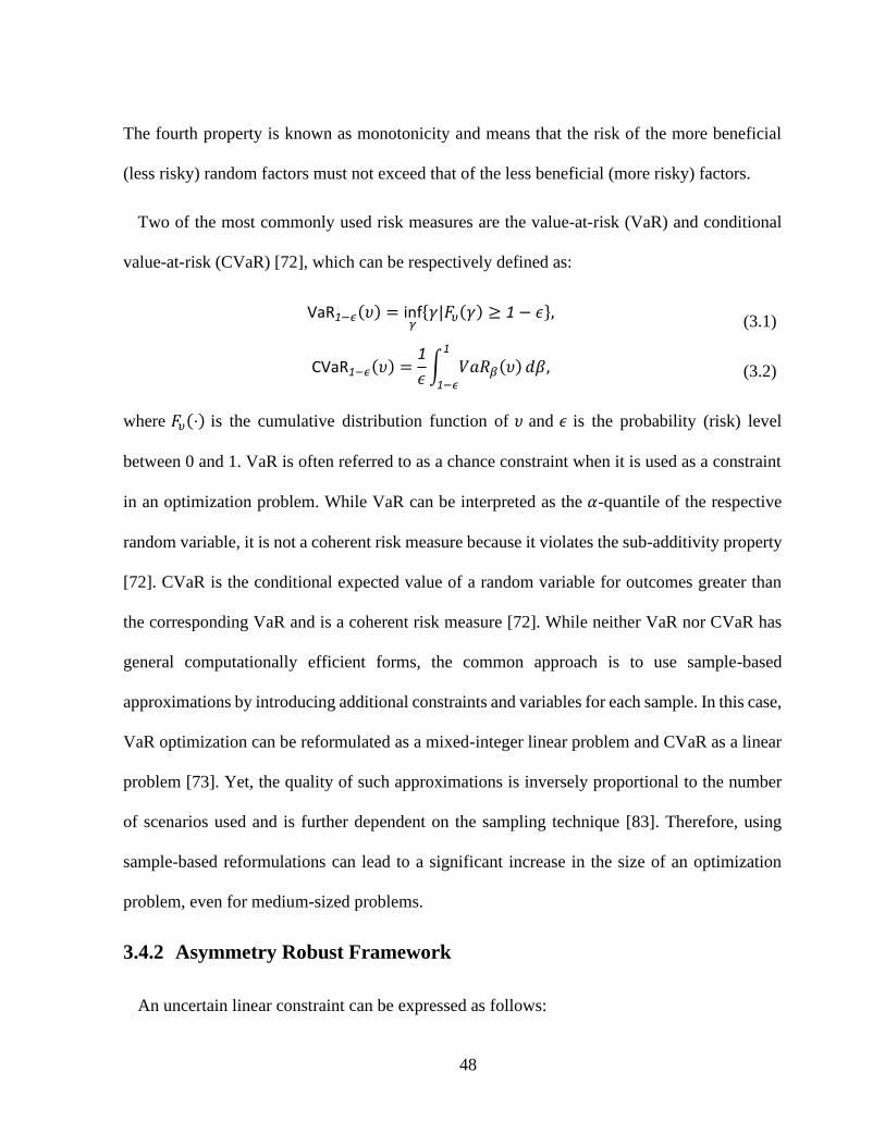
48
The fourth property is known as monotonicity and means that the risk of the more beneficial
(less risky) random factors must not exceed that of the less beneficial (more risky) factors.
Two of the most commonly used risk measures are the value-at-risk (VaR) and conditional
value-at-risk (CVaR) [72], which can be respectively defined as:
where 𝐹𝜐(⋅) is the cumulative distribution function of 𝜐 and 𝜖 is the probability (risk) level
between 0 and 1. VaR is often referred to as a chance constraint when it is used as a constraint
in an optimization problem. While VaR can be interpreted as the 𝛼-quantile of the respective
random variable, it is not a coherent risk measure because it violates the sub-additivity property
[72]. CVaR is the conditional expected value of a random variable for outcomes greater than
the corresponding VaR and is a coherent risk measure [72]. While neither VaR nor CVaR has
general computationally efficient forms, the common approach is to use sample-based
approximations by introducing additional constraints and variables for each sample. In this case,
VaR optimization can be reformulated as a mixed-integer linear problem and CVaR as a linear
problem [73]. Yet, the quality of such approximations is inversely proportional to the number
of scenarios used and is further dependent on the sampling technique [83]. Therefore, using
sample-based reformulations can lead to a significant increase in the size of an optimization
problem, even for medium-sized problems.
3.4.2 Asymmetry Robust Framework
An uncertain linear constraint can be expressed as follows:
VaR1−𝜖(𝜐) = inf𝛾
{𝛾|𝐹𝜐(𝛾) ≥ 1 − 𝜖}, (3.1)
CVaR1−𝜖(𝜐) =1
𝜖∫ 𝑉𝑎𝑅𝛽(𝜐)
1
1−𝜖
𝑑𝛽, (3.2)

49
where 𝒙 is the vector of decision variables and (��, b) is the vector of uncertain coefficients. The
uncertain coefficients can then be expressed in terms of underlying independent random
variables:
where (𝐚𝟎, b0) are the nominal values of the coefficients and (𝚫𝐚𝐣,Δbj) are the uncertainty
contributions of N underlying independent random variables z𝑗 . Each random variable z𝑗 is
assumed to have zero mean and support of [−z𝑗, z𝑗], with z
𝑗, z𝑗 > 0 being its lower and upper
bounds, respectively.
Each random variable z is assumed to belong to the asymmetric uncertainty set 𝒜, defined as
follows [74], [75]:
𝒜 = {𝐳 | ∃𝐯, 𝐰 ∈ 𝐑+N , 𝐳 = 𝐯 − 𝐰,
‖𝐏−1𝐯 + 𝐐−1𝐰‖ ≤Ω, −𝐳 ≤ 𝐳 ≤ 𝐳}, (3.5)
where 𝐳 is a vector of the random variables z𝑗, 𝐏 = diag(𝑝1, . . , 𝑝N) and 𝐐 = diag(𝑞1, . . , 𝑞N) are
the diagonal matrices of the forward and backward deviation measures respectively, and Ω is
the size of the uncertainty set, referred to as the uncertainty budget. The forward and backward
deviation measures generalize the standard deviation measure to capture the distributional
asymmetry. These deviation measures can be calculated directly from the data samples of the
random variable, from the moment generating functions of random variables, or approximated
in a distributionally robust way [74]. In this work, the data-based approach is utilized. Therefore,
��T𝒙 ≤ b, (3.3)
(��, b) = (𝐚𝟎, b0) + ∑(𝚫𝐚𝐣,Δbj)z𝑗
N
𝑗=1
, (3.4)

50
if a sample {𝑠(1), . . , 𝑠(𝑘)} of a random variable 𝑧 with sample mean �� is available, the forward
and backward deviations, 𝑝(𝑧) and 𝑞(𝑧), can be estimated using line search based on the
following expressions [84]:
An example of an asymmetric uncertainty set corresponding to random variables, 𝑧1 =
𝐵𝑒𝑡𝑎(1,5) and 𝑧2 = 𝐵𝑒𝑡𝑎(5,1), is shown in Figure 3.1 for various values of the uncertainty
budget.
Then, the uncertain constraint (3.3) can be included in an optimization problem by initially
replacing it with the corresponding VaR risk measure, commonly known as the chance
constraint:
P(��T𝒙 ≤ b) ≥ 1 − 𝜖 ↔ VaR1−𝜖(��T𝒙 − b) ≤ 0, (3.8)
where 𝜖 is the constraint violation probability level.
𝑝(z) = sup𝜃∈𝐑+
1
𝜃√2 ln
1
𝑘∑ exp(𝜃(𝑠(𝑖) − ��))
𝑘
𝑖=1
, (3.6)
𝑞(z) = sup𝜃∈𝐑+
1
𝜃√2 ln
1
𝑘∑ exp(−𝜃(𝑠(𝑖) − ��))
𝑘
𝑖=1
. (3.7)

51
Figure 3.1 Asymmetric Uncertainty Set Example
To overcome the abovementioned shortcomings of VaR, a robust optimization framework
based on an upper bound of VaR is proposed in [74], [75]. The robust reformulation of the
uncertain linear constraint VaR (3.8) with the asymmetric uncertainty set (3.5) is expressed as
follows:
For N underlying random variables, the robust reformulation requires the introduction of 3N
new variables, 2N new linear inequalities, and 1 conic inequality. Therefore, the reformulation
has a compact size and can be handled by commercial SOCP solvers. Note that the risk
𝐚𝟎T𝒙 +Ω‖𝒚‖2 + 𝒓T𝐳 + 𝒔T𝐳 ≤ b0, (3.9)
𝑦𝑗 ≥ 𝑝𝑗 (𝚫𝐚𝐣𝑻𝒙 −Δbj − 𝑟𝑗 + 𝑠𝑗) , ∀𝑗 = {1, . . , N}, (3.10)
𝑦𝑗 ≥ −𝑞𝑗 (𝚫𝐚𝐣𝑻𝒙 −Δbj − 𝑟𝑗 + 𝑠𝑗) , ∀𝑗 = {1, . . , N}, (3.11)
𝒚, 𝒓, 𝒔 ≥ 𝟎. (3.12)

52
contribution of each underlying random variable can be limited by its distributional support.
This enables the modeler to establish the connection between the physical range of the
underlying phenomena and its variability.
Moreover, asymmetry robust reformulation acts as an approximation of CVaR [75]. In fact,
while the size of the sample-based formulation of CVaR depends linearly on the number of
samples, the size of the asymmetry robust reformulation depends linearly on the number of
underlying random variables. Thus, when the number of random variables is significantly
smaller than the number of samples, the asymmetry robust reformulation can lead to a
considerable decrease in computational time, as is demonstrated in the case studies of Section
3.8.2.
The asymmetry robust reformulation provides an upper bound on the VaR problem, by
relating the constraint violation probability 𝜖 and the uncertainty budget Ω . The following
formula expresses this relation:
𝜖 = exp(−Ω2
2). (3.13)
Note that the independence assumption of underlying random variables z𝑗 in (3.4) is only
required to establish the relationship (3.13) between the uncertainty budget and constraint
violation probability. In fact, if a significant correlation exists between the underlying random
variables, it can be included by using a corresponding covariance matrix [75]. While all
coherency properties still hold in this case, the upper bound on risk (3.13) can only be used as
a reference.

53
The asymmetric uncertainty set is a generalization of the conventional symmetric uncertainty
set based on second moments and reduces to it in the case of symmetric distributions of
underlying random variables. Yet, the symmetric uncertainty set robust reformulation is not
coherent because the monotonicity property can be violated [75].
While the forecasting error distributions of many uncertain phenomena are symmetric,
conditional forecasts can be created by conditioning the random variable on some event, such
as belonging to a particular interval [85]. In turn, conditional forecasts usually have asymmetric
features, enabling uncertainty set parameters to be calculated for every conditional forecast
random variable and facilitating the coherency benefits of asymmetry robust framework.
3.5 Reformulation and Analysis of Power System Uncertainty Using
Coherent Risk Measures
3.5.1 Multiplicative Reformulation of Uncertain RESs
In the proposed approach, each RES is formulated as an adjustable power reference variable.
Then, in every uncertain inequality constraint each RES reference variable is multiplied by the
corresponding RES forecast random variable. In all equality constraints and inequality
constraints where uncertainty is negligible, each RES reference variable is multiplied by the
mean of its forecast random variable. Thus, for each RES 𝑟 a new optimization variable 𝑃𝑟,𝑡 is
introduced, corresponding to its scheduling decision at time 𝑡 . Variable 𝑃𝑟,𝑡 enters each
uncertain constraint multiplied by a contribution factor and by a random coefficient ��𝑟,𝑡
corresponding to the forecast random variable of RES 𝑟 at time 𝑡.
54
The RES scheduling variable 𝑃𝑟,𝑡 can be constrained between 0 and 1, resulting in the RES
being scheduled between zero and the nominal (mean) value of the forecast random variable
𝑃𝑟,𝑡0 . Alternatively, 𝑃𝑟,𝑡 can be constrained between 0 and 𝑃𝑟
max/𝑃𝑟,𝑡0 , enabling the RES to be
scheduled up to its full capacity. These approaches are referred to as “underscheduling” and
“overscheduling”, respectively. Note that RESs are considered schedulable only during the
operational planning problem for the purpose of risk management when their output is modeled
as random variables. During real-time operation, the output of RESs is still dependent on actual
weather conditions, but is assumed to be curtailable. Compared to “underscheduling”,
“overscheduling” increases the scheduling range of the RESs, which can lead to an increase in
their risk contributions above the nominal values of their forecast random variables. This can
result in more economical but riskier solutions, as demonstrated in the case studies later. The
use of “overscheduling” leads to the scheduling of more output from RESs and commitment of
fewer conventional units, consequently reducing the available operating reserves and increasing
the risk of their violation.
With respect to the uncertain linear constraint (3.3), each RES is modeled as an element of a
random coefficients vector ��, multiplied by the corresponding element of the decision vector 𝒙,
the former being the RES forecast random variable ��𝑟,𝑡 and the latter being the RES scheduling
variable 𝑃𝑟,𝑡. This is the main difference from most other approaches that treat RES forecast
uncertainty additively as the right-hand side uncontrollable random term b, thus influencing the
risk only through the translation invariance property and losing the benefits of the other
properties. The relationship between the properties of coherency and power system operational
planning is discussed next.
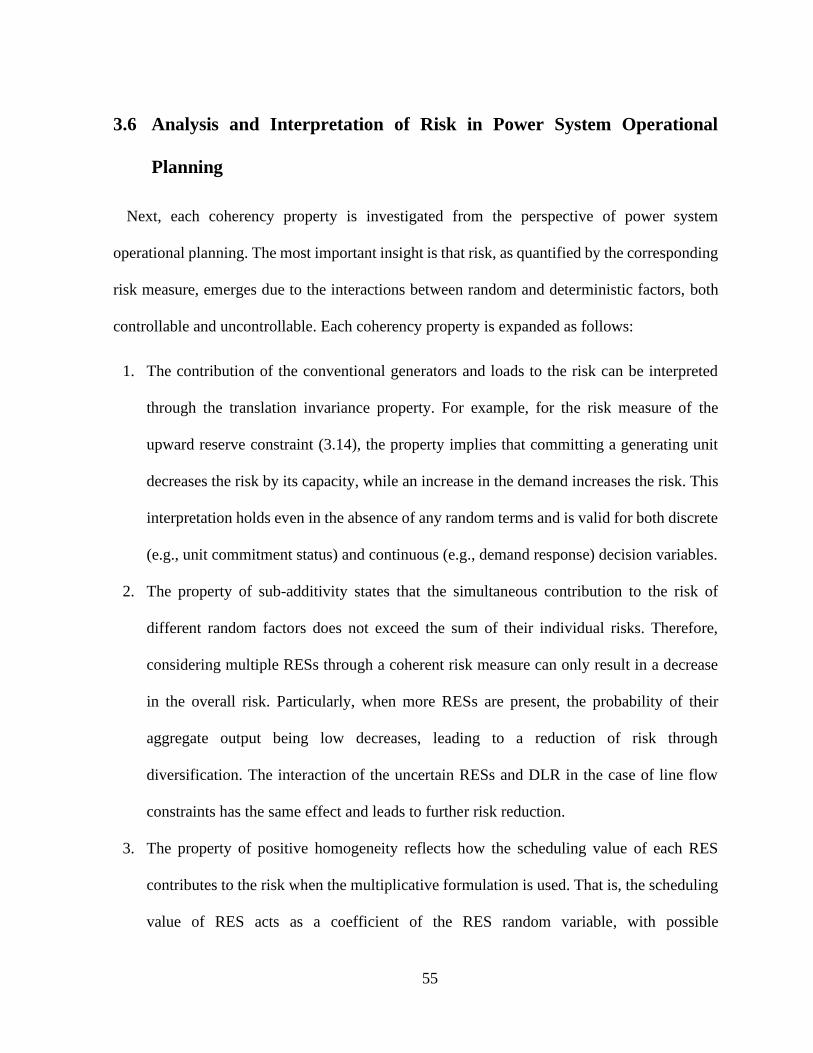
55
3.6 Analysis and Interpretation of Risk in Power System Operational
Planning
Next, each coherency property is investigated from the perspective of power system
operational planning. The most important insight is that risk, as quantified by the corresponding
risk measure, emerges due to the interactions between random and deterministic factors, both
controllable and uncontrollable. Each coherency property is expanded as follows:
1. The contribution of the conventional generators and loads to the risk can be interpreted
through the translation invariance property. For example, for the risk measure of the
upward reserve constraint (3.14), the property implies that committing a generating unit
decreases the risk by its capacity, while an increase in the demand increases the risk. This
interpretation holds even in the absence of any random terms and is valid for both discrete
(e.g., unit commitment status) and continuous (e.g., demand response) decision variables.
2. The property of sub-additivity states that the simultaneous contribution to the risk of
different random factors does not exceed the sum of their individual risks. Therefore,
considering multiple RESs through a coherent risk measure can only result in a decrease
in the overall risk. Particularly, when more RESs are present, the probability of their
aggregate output being low decreases, leading to a reduction of risk through
diversification. The interaction of the uncertain RESs and DLR in the case of line flow
constraints has the same effect and leads to further risk reduction.
3. The property of positive homogeneity reflects how the scheduling value of each RES
contributes to the risk when the multiplicative formulation is used. That is, the scheduling
value of RES acts as a coefficient of the RES random variable, with possible

56
implementations and their implications as discussed in Section 3.5.1. In the case of the
upward reserve constraint (3.14), the more (less) an RES is scheduled, the more (less) it
contributes to the risk. Consequently, if an RES is not scheduled (i.e., scheduled to zero),
then it does not contribute to the risk. This property is central to the proposed approach, as
it quantifies and allows control over the relationship between the value of the RES
scheduling and its risk contribution.
4. The monotonicity property states that, for a particular risk measure, random factors with
better outcomes should produce less risk. Together with the positive homogeneity
property, monotonicity ensures the prioritization of RESs with better outcomes (less risky)
in the overall schedule.
3.6.1 Asymmetry Robust Reformulation of the Uncertain Reserve
Constraints VaR
The uncertain constraint for upward reserve is defined as the requirement to satisfy the
demand by conventional generation and RESs. For every time period 𝑡 ∈ 𝓣, the constraint has
the following formulation:
∑ 𝑃𝑔,𝑡max𝑢𝑔,𝑡
𝑔∈𝓖
+ ∑ ��𝑟,𝑡𝑃𝑟,𝑡
𝑟∈𝓡
≥ ∑ 𝑃𝑑,𝑡
𝑑∈𝓓
. (3.14)
Then, the VaR of the uncertain upward reserve constraint (3.14) is reformulated according to
the asymmetry robust framework. Each RES forecast random variable, ��𝑟,𝑡 = 𝑃𝑟,𝑡0 + z𝑟,𝑡 ,
represents a random coefficient (3.4), which is modeled in terms of one underlying random
variable z𝑟,𝑡 and nominal (mean) value 𝑃𝑟,𝑡0 , giving the value of uncertainty contribution Δar,t

57
to be 1. In turn, z𝑟,𝑡 is the demeaned version of ��𝑟,𝑡, with 𝑃𝑟,𝑡, 𝑃𝑟,𝑡, 𝑝𝑟,𝑡, and 𝑞𝑟,𝑡 representing
the lower bound, upper bound, and forward and backward deviations of z𝑟,𝑡, respectively. While
all underlying random variables are assumed independent, any correlation between multiple
sources of uncertainty can be included accordingly [86].
By introducing auxiliary variables and corresponding parameters, constraint (3.14) is
transformed into the standard form (3.9)–(3.12), having the following reformulation:
where 𝑦𝑟,𝑡uw, 𝑟𝑟,𝑡
uw, 𝑠𝑟,𝑡uw are the robust counterpart, upper bound, and lower bound auxiliary
variables corresponding to the RES forecast random variable 𝑟 at time 𝑡 , respectively The
elements of the vector 𝒚𝑡uw are the variables 𝑦𝑗,𝑡
uw, and Ωuw is the upward reserve uncertainty
budget.
The uncertain constraint for downward reserve is defined as the requirement to utilize the
scheduled generation. For every time period 𝑡 ∈ 𝓣, the constraint has the following formulation:
∑ 𝑃𝑔,𝑡min𝑢𝑔,𝑡
𝑔∈𝓖
+ ∑ ��𝑟,𝑡𝑃𝑟,𝑡
𝑟∈𝓡
≤ ∑ 𝑃𝑑,𝑡
𝑑∈𝓓
. (3.19)
− ∑ 𝑃𝑔,𝑡max𝑢𝑔,𝑡
𝑔∈𝓖
− ∑ 𝑃𝑟,𝑡0 𝑃𝑟,𝑡
𝑟∈𝓡
+ ∑ 𝑃𝑑,𝑡
𝑑∈𝓓
+Ωuw‖𝒚𝑡uw‖2 + ∑ 𝑃𝑟,𝑡𝑟𝑟,𝑡
uw
𝑟∈𝓡
+ ∑ 𝑃𝑟,𝑡𝑠𝑟,𝑡uw
𝑟∈𝓡
≤ 0, (3.15)
𝑦𝑟,𝑡uw ≥ 𝑝𝑟,𝑡(−𝑃𝑟,𝑡 − 𝑟𝑟,𝑡
uw + 𝑠𝑟,𝑡uw), ∀𝑟 ∈ 𝓡, (3.16)
𝑦𝑟,𝑡uw ≥ −𝑞𝑟,𝑡(−𝑃𝑟,𝑡 − 𝑟𝑟,𝑡
uw + 𝑠𝑟,𝑡uw), ∀𝑟 ∈ 𝓡, (3.17)
𝑦𝑟,𝑡uw, 𝑟𝑟,𝑡
uw, 𝑠𝑟,𝑡uw ≥ 0, ∀𝑟 ∈ 𝓡, (3.18)

58
Analogously, the VaR of the downward reserve constraint has the following robust
reformulation:
where the notation is analogous to the upward reserve case.
3.6.2 Asymmetry Robust Reformulation of the Uncertain Line Flow
Constraints VaR
The uncertain linear line flow constraints, based on the DC network model, are defined as the
requirement to not exceed the line capacity for positive and negative power flows. For every
line monitored for DLR 𝑙 ∈ 𝓛𝐃 and every time period 𝑡 ∈ 𝓣, the constraints have the following
formulation:
−��𝑙,𝑡 ≤ ∑ 𝜋𝑙,𝑔𝑃𝑔,𝑡
𝑔∈𝓖
+ ∑ 𝜋𝑙,𝑟��𝑟,𝑡𝑃𝑟,𝑡
𝑟∈𝓡
− ∑ 𝜋𝑙,𝑑𝑃𝑑,𝑡
𝑑∈𝓓
≤ ��𝑙,𝑡. (3.24)
Similarly to the reserves constraints, each scaled RES forecast random variable 𝜋𝑙,𝑟��𝑟,𝑡 =
𝜋𝑙,𝑟𝑃𝑟,𝑡0 + 𝜋𝑙,𝑟 z𝑟,𝑡 represents a random coefficient (3.4) that is modeled in terms of one
underlying random variable z𝑟,𝑡 and nominal (mean) value 𝜋𝑙,𝑟𝑃𝑟,𝑡0 , giving the value of
uncertainty contribution Δar,t to be 𝜋𝑙,𝑟. The DLR uncertainty in the line flow constraints is
∑ 𝑃𝑔,𝑡min𝑢𝑔,𝑡
𝑔∈𝓖
+ ∑ 𝑃𝑟,𝑡0 𝑃𝑟,𝑡
𝑟∈𝓡
− ∑ 𝑃𝑑,𝑡
𝑑∈𝓓
+Ωdw‖𝒚𝑡dw‖
2+ ∑ 𝑃𝑟,𝑡𝑟𝑟,𝑡
dw
𝑟∈𝓡
+ ∑ 𝑃𝑟,𝑡𝑠𝑟,𝑡dw
𝑟∈𝓡
≤ 0, (3.20)
𝑦𝑟,𝑡dw ≥ 𝑝𝑟,𝑡(𝑃𝑟,𝑡 − 𝑟𝑟,𝑡
dw + 𝑠𝑟,𝑡dw), ∀𝑟 ∈ 𝓡, (3.21)
𝑦𝑟,𝑡dw ≥ −𝑞𝑟,𝑡(𝑃𝑟,𝑡 − 𝑟𝑟,𝑡
dw + 𝑠𝑟,𝑡dw), ∀𝑟 ∈ 𝓡, (3.22)
𝑦𝑟,𝑡dw, 𝑟𝑟,𝑡
dw, 𝑠𝑟,𝑡dw ≥ 0, ∀𝑟 ∈ 𝓡, (3.23)

59
modeled by introducing a forecast random variable ��𝑙,𝑡 = 𝑃𝑙,𝑡0 + z𝑙,𝑡 for the transmission line
capacity. The DLR forecast random variable ��𝑙,𝑡 is treated as the random right-hand side b due
to its uncontrollable nature.
Then, the VaR of the positive line flow constraint has the following robust reformulation:
where 𝑦𝑙,𝑟,𝑡pos , 𝑟𝑙,𝑟,𝑡
pos , 𝑠𝑙,𝑟,𝑡pos
are the robust counterpart, upper bound and lower bound auxiliary
variables for line 𝑙 for RES forecast random variable 𝑟 at time 𝑡 and 𝑦𝑙,𝑡pos, 𝑟𝑙,𝑡
pos, 𝑠𝑙,𝑡pos
are the
robust counterpart, upper bound, and lower bound auxiliary variables for the DLR forecast
random variable for line 𝑙 at time 𝑡. The elements of vector 𝒚𝑙,𝑡pos
are the variables 𝑦𝑙,𝑟,𝑡pos
and 𝑦𝑙,𝑡pos
,
and Ω𝑙 is the uncertainty budget for line 𝑙.
The VaR of the negative line flow constraint has the following robust reformulation:
∑ 𝜋𝑙,𝑔𝑃𝑔,𝑡
𝑔∈𝓖
+ ∑ 𝜋𝑙,𝑟𝑃𝑟,𝑡0 𝑃𝑟,𝑡
𝑟∈𝓡
− ∑ 𝜋𝑙,𝑑𝑃𝑑,𝑡
𝑑∈𝓓
+ Ω𝑙‖𝒚𝑙,𝑡pos‖
2+ ∑ 𝑃𝑟,𝑡𝑟𝑙,𝑟,𝑡
pos
𝑟∈𝓡
+ ∑ 𝑃𝑟,𝑡𝑠𝑙,𝑟,𝑡pos
𝑟∈𝓡
+ 𝑃𝑙,𝑡𝑟𝑙,𝑡pos + 𝑃𝑙,𝑡𝑠𝑙,𝑡
pos ≤ 𝑃𝑙,𝑡0 ,
(3.25)
𝑦𝑙,𝑡pos ≥ 𝑝𝑙,𝑡(−1 − 𝑟𝑙,𝑡
pos + 𝑠𝑙,𝑡pos), (3.26)
𝑦𝑙,𝑡pos ≥ −𝑞𝑙,𝑡(−1 − 𝑟𝑙,𝑡
pos + 𝑠𝑙,𝑡pos), (3.27)
𝑦𝑙,𝑟,𝑡pos ≥ 𝑝𝑟,𝑡(𝜋𝑙,𝑟𝑃𝑟,𝑡 − 𝑟𝑙,𝑟,𝑡
pos + 𝑠𝑙,𝑟,𝑡pos ), ∀𝑟 ∈ 𝓡, (3.28)
𝑦𝑙,𝑟,𝑡pos ≥ −𝑞𝑟,𝑡(𝜋𝑙,𝑟𝑃𝑟,𝑡 − 𝑟𝑙,𝑟,𝑡
pos + 𝑠𝑙,𝑟,𝑡pos ), ∀𝑟 ∈ 𝓡, (3.29)
𝑦𝑙,𝑡pos, 𝑟𝑙,𝑡
pos, 𝑠𝑙,𝑡pos ≥ 0, (3.30)
𝑦𝑙,𝑟,𝑡pos , 𝑟𝑙,𝑟,𝑡
pos , 𝑠𝑙,𝑟,𝑡pos , ≥ 0, ∀𝑟 ∈ 𝓡, (3.31)
− ∑ 𝜋𝑙,𝑔𝑃𝑔,𝑡
𝑔∈𝓖
− ∑ 𝜋𝑙,𝑟𝑃𝑟,𝑡0 𝑃𝑟,𝑡
𝑟∈𝓡
+ ∑ 𝜋𝑙,𝑑𝑃𝑑,𝑡
𝑑∈𝓓
(3.32)

60
where the notation is analogous to the positive case.
3.7 Risk-Averse Asymmetry Robust Unit Commitment
To demonstrate the use of coherent risk measures, the DC network-constrained UC problem
is chosen as a general example of an operational planning problem. A single-stage centralized
multi-period UC problem [87] is extended with the proposed robust reformulations of the
uncertain constraints. The equality constraints and the constraints where the uncertainty is
negligible are formulated with RES scheduling variable 𝑃𝑗,𝑡 being multiplied by the nominal
value of the RES forecast 𝑃𝑗,𝑡0 . The resulting UC problem formulation is as follows:
+𝛺𝑙‖𝒚𝑙,𝑡𝑛𝑒𝑔
‖2
+ ∑ 𝑃𝑟,𝑡𝑟𝑙,𝑟,𝑡𝑛𝑒𝑔
𝑟∈𝓡
+ ∑ 𝑃𝑟,𝑡𝑠𝑙,𝑟,𝑡𝑛𝑒𝑔
𝑟∈𝓡
+ 𝑃𝑙,𝑡𝑟𝑙,𝑡𝑛𝑒𝑔
+ 𝑃𝑙,𝑡𝑠𝑙,𝑡𝑛𝑒𝑔
≤ 𝑃𝑙,𝑡0 ,
𝑦𝑙,𝑡neg ≥ 𝑝𝑙,𝑡(−1 − 𝑟𝑙,𝑡
neg + 𝑠𝑙,𝑡neg), (3.33)
𝑦𝑙,𝑡neg ≥ −𝑞𝑙,𝑡(−1 − 𝑟𝑙,𝑡
neg + 𝑠𝑙,𝑡neg), (3.34)
𝑦𝑙,𝑟,𝑡neg ≥ 𝑝𝑟,𝑡(−𝜋𝑙,𝑟𝑃𝑟,𝑡 − 𝑟𝑙,𝑟,𝑡
neg + 𝑠𝑙,𝑟,𝑡neg ), ∀𝑟 ∈ 𝓡, (3.35)
𝑦𝑙,𝑟,𝑡neg ≥ −𝑞𝑟,𝑡(−𝜋𝑙,𝑟𝑃𝑟,𝑡 − 𝑟𝑙,𝑟,𝑡
neg + 𝑠𝑙,𝑟,𝑡neg ), ∀𝑟 ∈ 𝓡, (3.36)
𝑦𝑙,𝑡neg, 𝑟𝑙,𝑡
neg, 𝑠𝑙,𝑡neg ≥ 0, (3.37)
𝑦𝑙,𝑟,𝑡neg , 𝑟𝑙,𝑟,𝑡
neg , 𝑠𝑙,𝑟,𝑡neg ≥ 0, ∀𝑟 ∈ 𝓡, (3.38)
minimize∑ ∑(𝑓𝑔(𝑃𝑔,𝑡) + 𝑐𝑔su𝑣𝑔,𝑡 + 𝑐𝑔
sd𝑤𝑔,𝑡)
𝑔∈𝓖𝑡∈𝓣
, (3.39)
subject to
𝑣𝑔,𝑡 − 𝑤𝑔,𝑡 = 𝑢𝑔,𝑡 − 𝑢𝑔,𝑡−1, ∀𝑔 ∈ 𝓖, ∀𝑡 ∈ 𝓣, (3.40)
𝑃𝑔min𝑢𝑔,𝑡 ≤ 𝑃𝑔,𝑡 ≤ 𝑃𝑔
max𝑢𝑔,𝑡, ∀𝑔 ∈ 𝓖, ∀𝑡 ∈ 𝓣, (3.41)
𝑃𝑔,𝑡 − 𝑃𝑔,𝑡−1 ≤ 𝑅𝑔up𝑢𝑔,𝑡−1 + 𝑃𝑔
min𝑣𝑔,𝑡, (3.42)
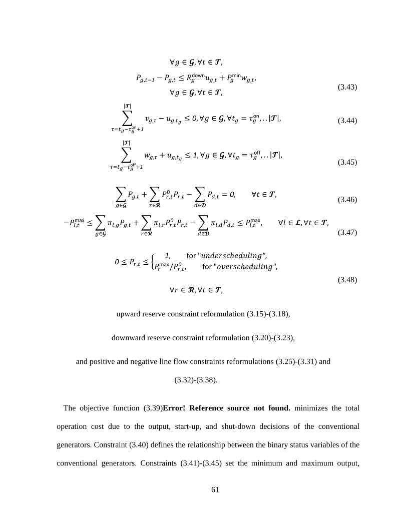
61
The objective function (3.39)Error! Reference source not found. minimizes the total
operation cost due to the output, start-up, and shut-down decisions of the conventional
generators. Constraint (3.40) defines the relationship between the binary status variables of the
conventional generators. Constraints (3.41)-(3.45) set the minimum and maximum output,
∀𝑔 ∈ 𝓖, ∀𝑡 ∈ 𝓣,
𝑃𝑔,𝑡−1 − 𝑃𝑔,𝑡 ≤ 𝑅𝑔down𝑢𝑔,𝑡 + 𝑃𝑔
min𝑤𝑔,𝑡,
∀𝑔 ∈ 𝓖, ∀𝑡 ∈ 𝓣, (3.43)
∑ 𝑣𝑔,𝜏
|𝓣|
𝜏=𝑡𝑔−𝜏𝑔on+1
− 𝑢𝑔,𝑡𝑔≤ 0, ∀𝑔 ∈ 𝓖, ∀𝑡𝑔 = 𝜏𝑔
on, . . |𝓣|, (3.44)
∑ 𝑤𝑔,𝜏
|𝓣|
𝜏=𝑡𝑔−𝜏𝑔off+1
+ 𝑢𝑔,𝑡𝑔≤ 1, ∀𝑔 ∈ 𝓖, ∀𝑡𝑔 = 𝜏𝑔
off, . . |𝓣|, (3.45)
∑ 𝑃𝑔,𝑡
𝑔∈𝓖
+ ∑ 𝑃𝑟,𝑡0 𝑃𝑟,𝑡
𝑟∈𝓡
− ∑ 𝑃𝑑,𝑡
𝑑∈𝓓
= 0, ∀𝑡 ∈ 𝓣, (3.46)
−𝑃𝑙,𝑡max ≤ ∑ 𝜋𝑙,𝑔𝑃𝑔,𝑡
𝑔∈𝓖
+ ∑ 𝜋𝑙,𝑟𝑃𝑟,𝑡0 𝑃𝑟,𝑡
𝑟∈𝓡
− ∑ 𝜋𝑙,𝑑𝑃𝑑,𝑡
𝑑∈𝓓
≤ 𝑃𝑙,𝑡max, ∀𝑙 ∈ 𝓛, ∀𝑡 ∈ 𝓣,
(3.47)
0 ≤ 𝑃𝑟,𝑡 ≤ {1, for "𝑢𝑛𝑑𝑒𝑟𝑠𝑐ℎ𝑒𝑑𝑢𝑙𝑖𝑛𝑔",
𝑃𝑟max/𝑃𝑟,𝑡
0 , for "𝑜𝑣𝑒𝑟𝑠𝑐ℎ𝑒𝑑𝑢𝑙𝑖𝑛𝑔",
∀𝑟 ∈ 𝓡, ∀𝑡 ∈ 𝓣,
(3.48)
upward reserve constraint reformulation (3.15)-(3.18),
downward reserve constraint reformulation (3.20)-(3.23),
and positive and negative line flow constraints reformulations (3.25)-(3.31) and
(3.32)-(3.38).

62
ramping capabilities, and minimum uptime and downtime for the conventional generators. The
energy balance equation is defined in (3.46) and conventional transmission line flow constraints
are defined in (3.47). The RES scheduling variable limits are set in (3.48) for one of the
described approaches and the robust reformulations of uncertain constraints are included
accordingly.
Consequently, the UC problem is expressed as a mixed-integer SOCP that can be directly
solved by commercial solvers.
3.8 Illustrative Example
3.8.1 Case Study Description
To illustrate the proposed framework, a 2019 update of the IEEE Reliability Test System,
referred to as RTS-GMLC, is used [88]. The system is assumed to have DLR technology
installed for transmission lines B3 (between buses 201 and 205) and C8 (between buses 304
and 309). The conductor types of both lines are assumed to be steel-reinforced aluminum
conductor “Falcon” 72/7 with the SLR set to 1354.6 A and a capacity of 175 MW. To be
consistent with other geographically based time series of RTS-GMLC, the weather data for the
DLR of lines B3 and C8 are assumed to come from Las Vegas and Los Angeles, respectively.
DarkSky weather service is used to acquire historical hourly weather data for the respective
locations for the years 2017-2019. For each line, the DLR time series for 2017 and 2018 are
used to train a neural network to produce 24-hour-ahead hourly forecasts, while the data from
2019 are used to produce the forecasts for the simulation. Then, DLR ampacity data are rescaled
to the MW capacity of the transmission lines.

63
In addition, the solar generation located on the same buses is aggregated, while concentrated
solar power and storage are not included. Conditional forecasts [85] are created with the number
of bins set at 12 and uncertainty set parameters are calculated for each conditional forecast bin.
The formulation is implemented in YALMIP [89] and the solutions are obtained using Gurobi
9.0 with a 0.1% optimality gap on an Intel i7-7700 PC with 12 GB of RAM.
3.8.2 Simulation Results
The performance of the proposed coherent risk-averse framework is demonstrated
numerically by comparing the following models, corresponding to different ways of handling
uncertainty:
1. Model A: Deterministic setting of reserves according to 3% of total demand and 5% of total
RES generation, known as the NREL 3+5 rule.
2. Model B: Gaussian reformulation of uncertain reserves (example 4.8 in [90], known as the
Markowitz portfolio problem) with “underscheduling” of RESs. RESs are modeled as
forecasted values and correlated error terms, similar to the methodology of [71].
3. Model C: Two-stage stochastic UC with 15 scenarios [16].
4. Model D: CVaR reformulation of uncertain reserves with “underscheduling” of RESs. A
sample-based reformulation with 1000 samples is used.
5. Model E: proposed asymmetry robust reformulation of uncertain reserves with
“overscheduling” of RESs.
6. Model F: proposed asymmetry robust reformulation of uncertain reserves with
“underscheduling” of RESs.
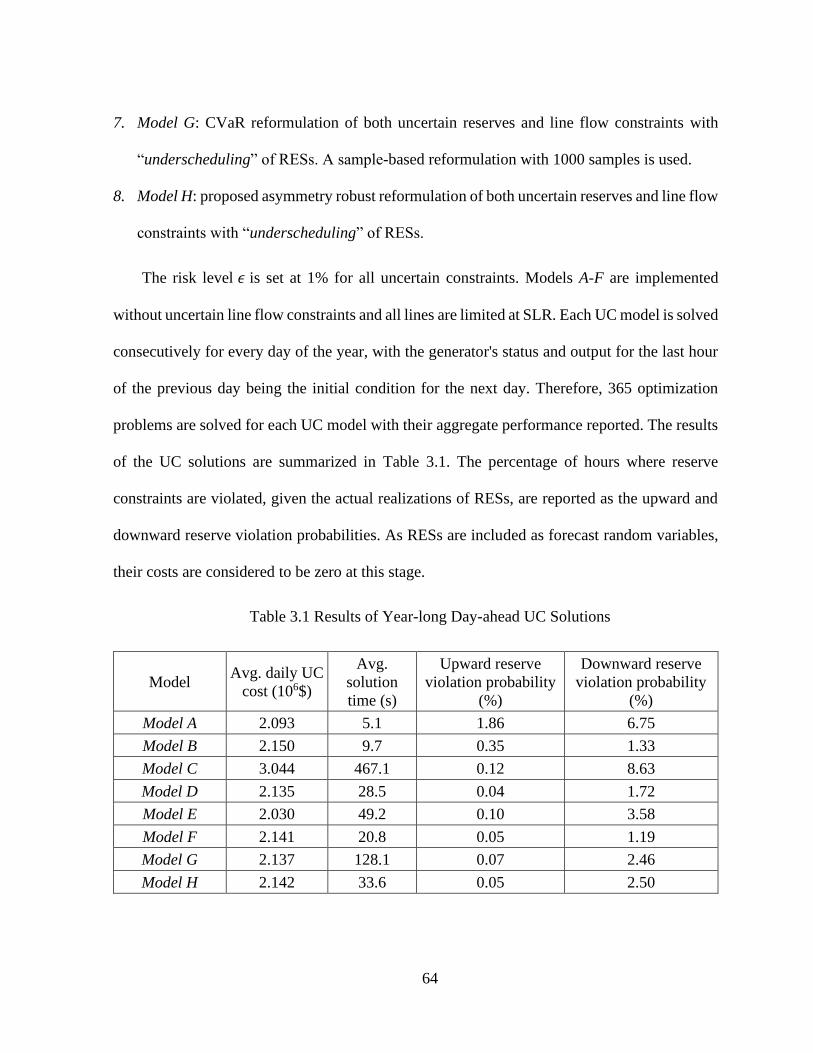
64
7. Model G: CVaR reformulation of both uncertain reserves and line flow constraints with
“underscheduling” of RESs. A sample-based reformulation with 1000 samples is used.
8. Model H: proposed asymmetry robust reformulation of both uncertain reserves and line flow
constraints with “underscheduling” of RESs.
The risk level 𝜖 is set at 1% for all uncertain constraints. Models A-F are implemented
without uncertain line flow constraints and all lines are limited at SLR. Each UC model is solved
consecutively for every day of the year, with the generator's status and output for the last hour
of the previous day being the initial condition for the next day. Therefore, 365 optimization
problems are solved for each UC model with their aggregate performance reported. The results
of the UC solutions are summarized in Table 3.1. The percentage of hours where reserve
constraints are violated, given the actual realizations of RESs, are reported as the upward and
downward reserve violation probabilities. As RESs are included as forecast random variables,
their costs are considered to be zero at this stage.
Table 3.1 Results of Year-long Day-ahead UC Solutions
Model Avg. daily UC
cost (106$)
Avg.
solution
time (s)
Upward reserve
violation probability
(%)
Downward reserve
violation probability
(%)
Model A 2.093 5.1 1.86 6.75
Model B 2.150 9.7 0.35 1.33
Model C 3.044 467.1 0.12 8.63
Model D 2.135 28.5 0.04 1.72
Model E 2.030 49.2 0.10 3.58
Model F 2.141 20.8 0.05 1.19
Model G 2.137 128.1 0.07 2.46
Model H 2.142 33.6 0.05 2.50

65
Among the single-stage models, the main difference in average daily UC costs primarily
comes from the scheduling method of RESs. In particular, the use of “overscheduling” instead
of “underscheduling” leads to a reduction in costs as a result of scheduling more output from
RESs. The average solution times of all single-stage models are also comparable, with Model A
being the fastest due to the simplicity of the model and Model G being the slowest due to the
additional variables and constraints of sample-based CVaR reformulation. For all risk-based
models, the reserves scheduled during the UC satisfy the risk requirements. Compared to the
single-stage models, two-stage stochastic Model C tends to commit a larger number of units,
resulting in higher costs and significantly longer solution times.
Furthermore, due to the presence of transmission congestion, the delivery of reserves is not
always possible. To simulate the delivery of reserves, a DC optimal power flow (OPF) based
on committed units with actual realizations of uncertain parameters is solved for each hour of
the year, for a total of 8760 instances. Results for the hourly DC OPF solutions are summarized
in Table 3.2. The cost associated with the curtailment of RESs is considered in the DC OPF and
set at 20 $/MW. As a result, the average hourly costs illustrated in Table 3.2 are different from
one twenty-fourth of the daily costs presented in Table 3.1, due to the forecasting errors in day-
ahead UC and the inclusion of RESs curtailment costs in hourly OPF. The percentage of all
OPF instances where load shedding occurs is reported as the insufficient generation probability,
indicating the probability of the risk. The average amount of load shedding in all such instances
is reported as the average insufficient generation, indicating the severity of the risk. The latter
risk metric is considered to be the most important, as it directly reflects the necessary amount
of corrective actions.

66
Table 3.2 Results of Year-long Hourly DC OPF Solutions
Model Avg. hourly
cost (103$)
Insufficient generation
probability (%)
Avg. insufficient
generation (MW)
Renewable
energy utilization
(%)
Model A 90.2 1.97 236.0 95.0
Model B 92.0 0.41 206.8 93.5
Model C 94.0 0.17 87.3 91.7
Model D 92.5 0.24 66.5 93.0
Model E 92.1 0.77 63.5 93.2
Model F 92.5 0.34 55.7 92.7
Model G 92.4 0.31 51.5 93.0
Model H 92.4 0.30 48.0 92.7
The effect of network congestion on the delivery of reserves is evident in the relative increase
of the probability of insufficient generation, compared to the UC results of Table 3.1. As
different models apply different reformulations of the reserves constraints, the risks associated
with the underlying random variables are evaluated differently, which leads to different UC
solutions resulting in different values and allocations of available reserves across the network
for each model. Consequently, the delivery of the reserves becomes different in real-time
operation to handle the uncertainties, leading to the given differences in performance
represented by the metrics in Table 3.2. The average hourly operating costs largely depend on
the conservativeness of the solution, with more conservative solutions committing more units
and leading to increased operating costs and limiting the ability to utilize available RES outputs.
Moreover, compared to other metrics, the risk metrics of average insufficient generation vary
by an order of magnitude with different models, indicating the necessity of prioritizing risk
management.

67
Comparing Models A through F without uncertain line flow constraints, Model A is the most
economical but does not directly manage risk and has the highest probability of generation
insufficiency at 1.97% and the worst average insufficient generation at 236.0 MW. While
managing the probability of the reserves violation compared to Model A, Model B lowers the
insufficient generation probability to 0.41% but fails to address the average insufficient
generation of 206.8 MW. This is the result of Model B being based on the Gaussian
reformulation, which is incapable of representing and addressing the tail properties of the
distributions. The result of Model B demonstrates that using the probability of constraint
violation alone is an insufficient indicator of the model’s risk managing properties. The two-
stage Model C results in the most conservative commitment decisions with the lowest
insufficient generation probability of 0.17% and the highest average operating cost. However,
Model C also does not directly address the average insufficient generation of 87.3 MW. Models
D and F with “underscheduling” have similar performance and demonstrate desirable risk
managing properties by addressing both the probability and average value of the insufficient
generation. Model E implements the proposed approach with “overscheduling” to better utilize
RESs and results in a relatively high probability of insufficient generation of 0.77%.
As discussed in Section 3.5, if the RESs are modeled multiplicatively, enabling the positive
homogeneity property, their scheduled output directly affects the risk of constraint violation.
The comparison of Models E and F shows the difference between modeling RESs with
“underscheduling” and “overscheduling”. The use of “overscheduling” allows the scheduling
of RES outputs above their nominal forecast values (with the corresponding increase in risk),
replacing conventional generation in the UC solutions. While the overall risk is limited by the
uncertainty budget Ω , it can still increase, compared to the “underscheduling” case.

68
Consequently, as the increase in risk is more significant than the decrease in cost, it can be
concluded that scheduling RESs above their nominal forecast values is disadvantageous from
the risk-averse perspective and “underscheduling” should be preferred.
The benefits of including uncertain line flow constraints with DLR are shown by Models G
and H. Model H has the smallest average value of insufficient generation at 48.0 MW and
demonstrates a 3.8-fold decrease in average solution time compared to Model G.
It must be further stressed that more than 1000 samples must be used to achieve a high
certainty level of the CVaR solution. Using the results of [83], the lower theoretical bound on
the number of samples to ensure a 1% risk level with a certainty level of 99.999% can be
calculated. In the system employed, each uncertain constraint has 114 decision variables,
requiring 2/0.01 ⋅ (ln(1 − 0.99999)−1 + 114) ≈ 25000 samples. This would result in
practically unacceptable UC solution times of CVaR reformulation, especially if a large number
of transmission lines with uncertain line flow constraints are considered.
As our year-long simulation covers a wide range of operating scenarios, the results obtained
can be treated with high fidelity. The results demonstrate how the proposed framework is
capable of significantly lowering the probability and magnitude of undesirable events due to the
coherent formulation of uncertainty and active scheduling of RESs. If the solution time is not
critical, the CVaR approach can be recommended as a single-stage model, or a two-stage model
can be extended using the proposed methodology to additionally address the magnitude of
undesirable events. Otherwise, the asymmetry robust reformulation should be preferred, as it
provides faster, more economical, and the most risk-averse solutions.

69
3.8.3 Impact of Risk Level
While the uncertainty budget (3.13) corresponding to the predefined risk level provides an
upper bound on constraint violation, the selection of the uncertainty budget can also be
performed based on the actual performance. Thus, the simulation of Model F from Section 3.8.2
is repeated with different risk levels between 0.5 and 5%. The results of the hourly DC OPF
solutions are summarized in Table 3.3.
Table 3.3 Impact of Risk Level on the Hourly DC OPF Solutions
Predefined
Risk level
(%)
Avg. hourly
cost (103$)
Insufficient generation
probability (%)
Avg. insufficient
generation (MW)
Renewable
energy utilization
(%)
0.5 92.7 0.29 55.3 92.7
1 92.5 0.34 55.7 92.7
2 92.5 0.39 52.3 92.8
3 92.2 0.19 47.4 93.0
4 92.2 0.36 57.3 93.0
5 92.3 0.49 66.1 93.1
Based on the results of Table 3.3, it can be concluded that the uncertainty budget
corresponding to the predefined risk level of 3% provides the best performance based on all
considered metrics. Note that the best value of the uncertainty budget is determined for the RTS-
GMLC test system data when the number of bins for conditional random variables is set at 12,
but it can be different for other input parameters and should be determined accordingly.
3.8.4 ACTIVSg2000 Test Case
To demonstrate the scalability and effectiveness of the proposed framework on a large-scale
system, the case study is extended to the ACTIVSg2000 test case [91]. ACTIVSg2000 is a
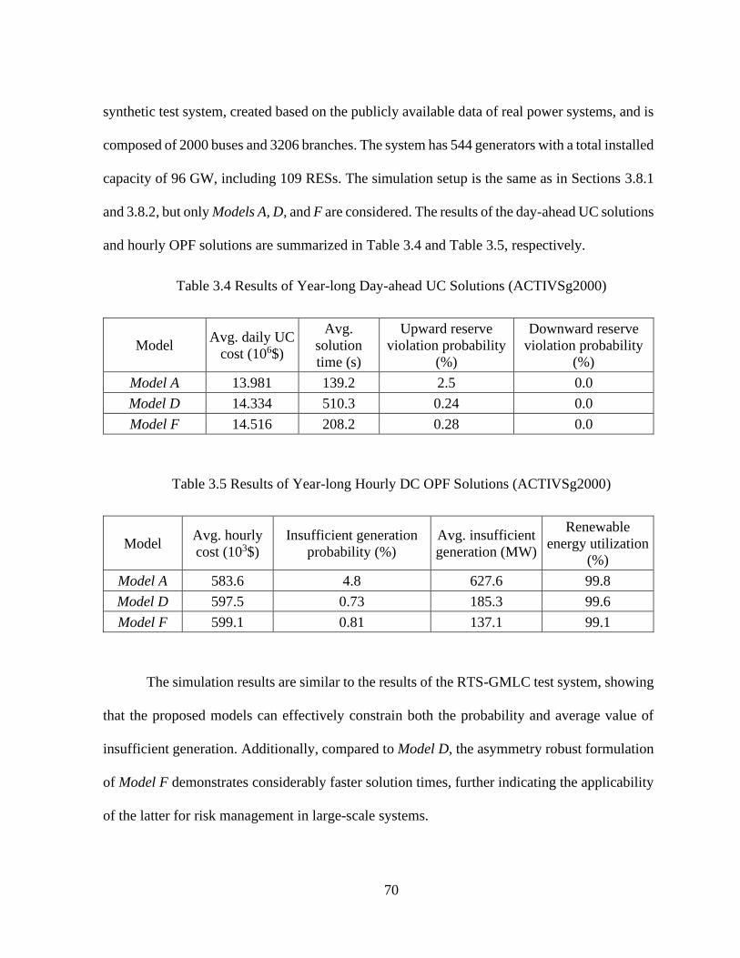
70
synthetic test system, created based on the publicly available data of real power systems, and is
composed of 2000 buses and 3206 branches. The system has 544 generators with a total installed
capacity of 96 GW, including 109 RESs. The simulation setup is the same as in Sections 3.8.1
and 3.8.2, but only Models A, D, and F are considered. The results of the day-ahead UC solutions
and hourly OPF solutions are summarized in Table 3.4 and Table 3.5, respectively.
Table 3.4 Results of Year-long Day-ahead UC Solutions (ACTIVSg2000)
Model Avg. daily UC
cost (106$)
Avg.
solution
time (s)
Upward reserve
violation probability
(%)
Downward reserve
violation probability
(%)
Model A 13.981 139.2 2.5 0.0
Model D 14.334 510.3 0.24 0.0
Model F 14.516 208.2 0.28 0.0
Table 3.5 Results of Year-long Hourly DC OPF Solutions (ACTIVSg2000)
Model Avg. hourly
cost (103$)
Insufficient generation
probability (%)
Avg. insufficient
generation (MW)
Renewable
energy utilization
(%)
Model A 583.6 4.8 627.6 99.8
Model D 597.5 0.73 185.3 99.6
Model F 599.1 0.81 137.1 99.1
The simulation results are similar to the results of the RTS-GMLC test system, showing
that the proposed models can effectively constrain both the probability and average value of
insufficient generation. Additionally, compared to Model D, the asymmetry robust formulation
of Model F demonstrates considerably faster solution times, further indicating the applicability
of the latter for risk management in large-scale systems.

71
3.9 Conclusion
This work proposes a risk-averse operational planning framework based on coherent risk
measures to manage the risk due to uncertainty from RESs and DLR. It presents an analysis of
power system operational planning risk and develops a novel formulation of uncertain RESs,
allowing them to be scheduled coherently along with other sources of uncertainty.
Year-long case studies are performed to evaluate different approaches to risk management in
the presence of network congestion, highlighting the need to focus on the delivery of the
reserves and not only on the total amount. Compared to other approaches, the models based on
the coherent framework are the most effective at managing the probability and magnitude of
undesirable events, reducing such risk metrics by an order of magnitude. The inclusion of DLR
is shown to further facilitate the delivery of reserves. In addition, the proposed asymmetry
robust reformulation of uncertain constraints is shown to be scalable and computationally
efficient, proving its usefulness in practical risk management problems.

72
4 Conclusions and Future Work
This thesis has investigated the impacts of unceratainty of DLR forecasts on the power
system operational planning. The research highlights the benefits and challenges of utilizing
DLR technologies and proposes new models to manage the operational risk in an efficient and
secure way. The main contributions and findings of this thesis are summarized in the following
list:
• The development of stochastic models for DLR that can be used in operational planning
problems for the risk-averse control of conductor temperature dynamics. Additionally,
the necessity to consider both the probability and the magnitude of the events of thermal
overloading of conductors monitored under DLR is accentuated.
• The analysis of uncertain factors and their interactions in operational planning problems
using coherent risk measures. The analysis highlights how different factors affect the
risk and how the risk management can be interpreted and managed from the power
system operator’s perspective. Furthermore, a new model for the renewable energy
sources in operational planning problems is proposed. Additionally, coherent
reformulations of uncertain reserves and line flow constraints are developed. These
constraints are included into the novel formulation of UC, that allows to perform the
scheduling in a coherent way, considering multiple sources of uncertainty.
Finally, the results of this thesis can be extended and investigated in several directions. First,
the impacts of extreme and rare weather conditions can be included in DLR models. However,
this line of future work would likely require the construction of more sophisticated simulation
methods, e.g. computational fluid dynamics, instead of solely relying on historical

73
measurements. Secondly, the potential of using energy storage systems together with the DLR
technologies and wind power should be further researched in both operational and expansion
planning problems. In particular, due to the correlations between the DLR, wind speed and wind
power, it is envisaged that properly designed and managed energy storage systems can mitigate
the associated uncertainties and lead to net benefits.

74
References
[1] C. Bussar et al., “Large-scale integration of renewable energies and impact on storage
demand in a European renewable power system of 2050-Sensitivity study,” J. Energy
Storage, vol. 6, pp. 1–10, 2016.
[2] A. Singh, T. Frei, N. Chokani, and R. S. Abhari, “Impact of unplanned power flows in
interconnected transmission systems – Case study of Central Eastern European region,”
Energy Policy, vol. 91, pp. 287–303, 2016.
[3] T. Sousa, T. Soares, P. Pinson, F. Moret, T. Baroche, and E. Sorin, “Peer-to-peer and
community-based markets: A comprehensive review,” Renew. Sustain. Energy Rev., vol.
104, no. January, pp. 367–378, 2019.
[4] M. Zugno, S. Member, P. Pinson, S. Member, and H. Madsen, “Impact of Wind Power
Generation on European Cross-Border Power Flows,” IEEE Trans. Power Syst., vol. 28,
no. 4, pp. 3566–3575, 2013.
[5] R. A. Rodríguez, S. Becker, G. B. Andresen, D. Heide, and M. Greiner, “Transmission
needs across a fully renewable European power system,” Renew. Energy, vol. 63, pp.
467–476, 2014.
[6] D. Douglass et al., “Real-Time Overhead Transmission-Line Monitoring for Dynamic
Rating,” IEEE Trans. Power Deliv., vol. 31, no. 3, pp. 921–927, 2016.
[7] S. Karimi, P. Musilek, and A. M. Knight, “Dynamic thermal rating of transmission lines :
A review,” Renew. Sustain. Energy Rev., vol. 91, no. March, pp. 600–612, 2018.
[8] B. P. Bhattarai et al., “Improvement of Transmission Line Ampacity Utilization by

75
Weather-Based Dynamic Line Rating,” IEEE Trans. Power Deliv., vol. 33, no. 4, pp.
1853–1863, 2018.
[9] C. J. Wallnerström, Y. Huang, and S. Member, “Impact From Dynamic Line Rating on
Wind Power Integration,” IEEE Trans. Smart Grid, vol. 6, no. 1, pp. 343–350, 2015.
[10] R. Dupin, L. Cavalcante, R. J. Bessa, G. Kariniotakis, and A. Michiorri, “Extreme
Quantiles Dynamic Line Rating Forecasts and Application on Network Operation,”
Energies, vol. 13, no. 12, p. 3090, 2020.
[11] A. Safdarian, M. Z. Degefa, M. Fotuhi-Firuzabad, and M. Lehtonen, “Benefits of Real-
Time Monitoring to Distribution Systems: Dynamic Thermal Rating,” IEEE Trans.
Smart Grid, vol. 6, no. 4, pp. 2023–2031, 2015.
[12] D. M. Greenwood and P. C. Taylor, “Investigating the impact of real-time thermal ratings
on power network reliability,” IEEE Trans. Power Syst., vol. 29, no. 5, pp. 2460–2468,
2014.
[13] H. Sugihara, T. Funaki, and N. Yamaguchi, “Evaluation method for real-time dynamic
line ratings based on line current variation model for representing forecast error of
intermittent renewable generation,” Energies, vol. 10, no. 4, 2017.
[14] M. M. Esfahani and G. R. Yousefi, “Real Time Congestion Management in Power
Systems Considering Quasi-Dynamic Thermal Rating and Congestion Clearing Time,”
IEEE Trans. Ind. Informatics, vol. 12, no. 2, pp. 745–754, 2016.
[15] T. Ringelband, P. Schäfer, and A. Moser, “Probabilistic ampacity forecasting for
overhead lines using weather forecast ensembles,” Electr. Eng., vol. 95, no. 2, pp. 99–

76
107, 2013.
[16] F. Teng, R. Dupin, A. Michiorri, G. Kariniotakis, Y. Chen, and G. Strbac,
“Understanding the Benefits of Dynamic Line Rating Under Multiple Sources of
Uncertainty,” IEEE Trans. Power Syst., vol. 33, no. 3, pp. 3306–3314, 2018.
[17] M. A. Bucher and G. Andersson, “Robust Corrective Control Measures in Power Systems
with Dynamic Line Rating,” IEEE Trans. Power Syst., vol. 31, no. 3, pp. 2034–2043,
2016.
[18] P. Kundur, Power system stability and control. New York: McGraw-hill, 1994.
[19] “IEEE standard for calculating the current-temperature relationship of bare overhead
conductors, IEEE Std 738,” 2013.
[20] “Guide for thermal rating calculations of overhead lines,” CIGRE, 2014.
[21] A. Arroyo et al., “Comparison between IEEE and CIGRE thermal behaviour standards
and measured temperature on a 132-kV overhead power line,” Energies, vol. 8, no. 12,
pp. 13660–13671, 2015.
[22] D. J. Morrow, J. Fu, and S. M. Abdelkader, “Experimentally validated partial least
squares model for dynamic line rating,” IET Renew. Power Gener., vol. 8, no. 3, pp. 260–
268, 2014.
[23] E. Fernandez, I. Albizu, M. T. Bedialauneta, A. J. Mazon, and P. T. Leite, “Review of
dynamic line rating systems for wind power integration,” Renew. Sustain. Energy Rev.,
vol. 53, no. 2016, pp. 80–92, 2020.
[24] J. Yang, X. Bai, D. Strickland, L. Jenkins, and A. M. Cross, “Dynamic network rating

77
for low carbon distribution network operation - A U.K. application,” IEEE Trans. Smart
Grid, vol. 6, no. 2, pp. 988–998, 2015.
[25] L. Dawson and A. M. Knight, “Applicability of Dynamic Thermal Line Rating for Long
Lines,” IEEE Trans. Power Deliv., vol. 33, no. 2, pp. 719–727, 2018.
[26] M. Matus et al., “Identification of critical spans for monitoring systems in dynamic
thermal rating,” IEEE Trans. Power Deliv., vol. 27, no. 2, pp. 1002–1009, 2012.
[27] J. Teh and I. Cotton, “Critical span identification model for dynamic thermal rating
system placement,” IET Gener. Transm. Distrib., vol. 9, no. 16, pp. 2644–2652, 2015.
[28] A. Michiorri, P. C. Taylor, and S. C. E. Jupe, “Overhead line real-time rating estimation
algorithm: Description and validation,” Proc. Inst. Mech. Eng. Part A J. Power Energy,
vol. 224, no. 3, pp. 293–304, 2010.
[29] D. L. Alvarez, F. Faria da Silva, E. E. Mombello, C. L. Bak, J. A. Rosero, and D. L.
Ólason, “An approach to dynamic line rating state estimation at thermal steady state using
direct and indirect measurements,” Electr. Power Syst. Res., 2017.
[30] A. W. Abboud, J. P. Gentle, T. R. McJunkin, and J. P. Lehmer, “Using Computational
Fluid Dynamics of Wind Simulations Coupled with Weather Data to Calculate Dynamic
Line Ratings,” IEEE Trans. Power Deliv., vol. 35, no. 2, pp. 745–753, 2020.
[31] D. M. Greenwood, G. L. Ingram, and P. C. Taylor, “Applying Wind Simulations for
Planning and Operation of Real-Time Thermal Ratings,” IEEE Trans. Smart Grid, vol.
8, no. 2, pp. 537–547, 2017.
[32] P. C. Taylor and D. M. Greenwood, “Unlocking the benefits of real-time thermal ratings

78
through probabilistic power network planning,” IET Gener. Transm. Distrib., vol. 8, no.
12, pp. 2055–2064, 2014.
[33] J. Zhan, W. Liu, and C. Y. Chung, “Stochastic Transmission Expansion Planning
Considering Uncertain Dynamic Thermal Rating of Overhead Lines,” IEEE Trans.
Power Syst., vol. 34, no. 1, pp. 432–443, 2019.
[34] H. Shaker, H. Zareipour, and M. Fotuhi-Firuzabad, “Reliability modeling of dynamic
thermal rating,” IEEE Trans. Power Deliv., vol. 28, no. 3, pp. 1600–1609, 2013.
[35] J. Teh, “Reliability Impacts of the Dynamic Thermal Rating System on Smart Grids
Considering Wireless Communications,” IEEE Access, vol. 7, pp. 41625–41635, 2019.
[36] A. Michiorri et al., “Forecasting for dynamic line rating,” Renew. Sustain. Energy Rev.,
vol. 52, pp. 1713–1730, 2015.
[37] D. A. Douglass et al., “A review of dynamic thermal line rating methods with
forecasting,” IEEE Trans. Power Deliv., vol. 34, no. 6, pp. 2100–2109, 2019.
[38] J. Zhan, C. Y. Chung, and E. Demeter, “Time Series Modeling for Dynamic Thermal
Rating of Overhead Lines,” IEEE Trans. Power Syst., vol. 32, no. 3, pp. 2172–2182,
2017.
[39] F. Fan, K. Bell, and D. Infield, “Probabilistic Real-Time Thermal Rating Forecasting for
Overhead Lines by Conditionally Heteroscedastic Auto-Regressive Models,” IEEE
Trans. Power Deliv., vol. 32, no. 4, pp. 1881–1890, 2017.
[40] F. Fan, K. Bell, and D. Infield, “Transient-state real-time thermal rating forecasting for
overhead lines by an enhanced analytical method,” Electr. Power Syst. Res., vol. 167, no.

79
October 2018, pp. 213–221, 2019.
[41] I. Albizu, E. Fernandez, A. J. Mazon, and R. Alberdi, “Forecast ratio and security
analysis of rating forecasting methods in an overhead line,” IET Gener. Transm. Distrib.,
vol. 11, no. 6, pp. 1598–1604, 2017.
[42] N. Siebert, “Dynamic Line Rating Using Numerical Weather Predictions and Machine
Learning : A Case Study,” IEEE Trans. Power Deliv., vol. 32, no. 1, pp. 335–343, 2017.
[43] C. Wang, R. Gao, F. Qiu, J. Wang, and L. Xin, “Risk-based distributionally robust
optimal power flow with dynamic line rating,” IEEE Trans. Power Syst., vol. 33, no. 6,
pp. 6074–6086, 2018.
[44] D. Fang, M. Zou, G. Coletta, A. Vaccaro, and S. Z. Djokic, “Handling uncertainties with
affine arithmetic and probabilistic OPF for increased utilisation of overhead transmission
lines,” Electr. Power Syst. Res., vol. 170, no. January, pp. 364–377, 2019.
[45] J. Cao, W. Du, and H. F. Wang, “Weather-Based Optimal Power Flow with Wind Farms
Integration,” IEEE Trans. Power Syst., vol. 31, no. 4, pp. 3073–3081, 2016.
[46] B. O. Ngoko, H. Sugihara, and T. Funaki, “Optimal power flow considering line-
conductor temperature limits under high penetration of intermittent renewable energy
sources,” Int. J. Electr. Power Energy Syst., vol. 101, no. March, pp. 255–267, 2018.
[47] Y. Wang, Z. Sun, Z. Yan, L. Liang, and F. Song, “Power Transmission Congestion
Management Based on Quasi-Dynamic Thermal Rating,” Processes, vol. 7, no. 5, p. 244,
2019.
[48] J. S. A. Carneiro and L. Ferrarini, “Preventing thermal overloads in transmission circuits

80
via model predictive control,” IEEE Trans. Control Syst. Technol., vol. 18, no. 6, pp.
1406–1412, 2010.
[49] B. Banerjee, D. Jayaweera, and S. Islam, “Risk constrained short-term scheduling with
dynamic line ratings for increased penetration of wind power,” Renew. Energy, vol. 83,
pp. 1139–1146, 2015.
[50] H. Park, Y. G. Jin, and J. K. Park, “Stochastic security-constrained unit commitment with
wind power generation based on dynamic line rating,” Int. J. Electr. Power Energy Syst.,
vol. 102, no. April, pp. 211–222, 2018.
[51] J. Shi and S. S. Oren, “Flexible line ratings in stochastic unit commitment for power
systems with large-scale renewable generation,” Energy Syst., 2018.
[52] R. Dupin, A. Michiorri, and G. Kariniotakis, “Optimal Dynamic Line Rating Forecasts
Selection Based on Ampacity Probabilistic Forecasting and Network Operators’ Risk
Aversion,” IEEE Trans. Power Syst., pp. 1–1, 2019.
[53] Y. Li et al., “Day-ahead Scheduling of Power System Incorporating Network Topology
Optimization and Dynamic Thermal Rating,” IEEE Access, pp. 1–1, 2019.
[54] M. Nick, O. Alizadeh-Mousavi, R. Cherkaoui, and M. Paolone, “Security Constrained
Unit Commitment with Dynamic Thermal Line Rating,” IEEE Trans. Power Syst., vol.
31, no. 3, pp. 2014–2025, 2016.
[55] M. R. Almassalkhi and I. A. Hiskens, “Model-predictive cascade mitigation in electric
power systems with storage and renewables - PARt II: Case-study,” IEEE Trans. Power
Syst., vol. 30, no. 1, pp. 78–87, 2015.

81
[56] J. Fu, D. J. Morrow, and S. M. Abdelkader, “Modelling and Prediction Techniques for
Dynamic Overhead Line Rating,” Power Energy Soc. Gen. Meet., pp. 1–7, 2012.
[57] C. Bishop, Pattern Recognition and Machine Learning, 1st ed. New York, NY, USA:
Springer, 2011.
[58] R. Koenker, Quantile Regression. Cambridge University Press, 2005.
[59] X. Sun, P. B. Luh, K. W. Cheung, and W. Guan, “Probabilistic forecasting of dynamic
line rating for over-head transmission lines,” IEEE Power Energy Soc. Gen. Meet., vol.
2015-Septe, 2015.
[60] R. T. Rockafellar, J. O. Royset, and S. I. Miranda, “Superquantile regression with
applications to buffered reliability, uncertainty quantification, and conditional value-at-
risk,” Eur. J. Oper. Res., vol. 234, no. 1, pp. 140–154, 2014.
[61] P. Kall and J. Mayer, Stochastic Linear Programming: Models, Theory, and
Computation, 2nd ed. New York: Springer US, 2011.
[62] C. Ordoudis, P. Pinson, J. M. Morales-González, and M. Zugno, “An Updated Version
of the IEEE RTS 24-Bus System for Electricity Market and Power System Operation
Studies,” Tech. Univ. Denmark, 2016, [Online]. Available:
https://backend.orbit.dtu.dk/ws/portalfiles/portal/120568114/An_Updated_Version_of_
the_IEEE_RTS_24Bus_System_for_Electricty_Market_an....pdf.
[63] L. Badesa, F. Teng, and G. Strbac, “Simultaneous scheduling of multiple frequency
services in stochastic unit commitment,” IEEE Trans. Power Syst., vol. 34, no. 5, pp.
3858–3868, Sep. 2019.

82
[64] M. Paturet, U. Markovic, S. Delikaraoglou, E. Vrettos, P. Aristidou, and G. Hug,
“Stochastic unit commitment in low-inertia grids,” IEEE Trans. Power Syst., vol. 35, no.
5, pp. 3448–3458, Sep. 2020.
[65] Á. Lorca, X. A. Sun, E. Litvinov, and T. Zheng, “Multistage adaptive robust optimization
for the unit commitment problem,” Oper. Res., vol. 64, no. 1, pp. 32–51, Jan. 2016.
[66] I. Blanco and J. M. Morales, “An efficient robust solution to the two-stage stochastic unit
commitment problem,” IEEE Trans. Power Syst., vol. 32, no. 6, pp. 4477–4488, Nov.
2017.
[67] P. Xiong, P. Jirutitijaroen, and C. Singh, “A Distributionally Robust Optimization Model
for Unit Commitment Considering Uncertain Wind Power Generation,” IEEE Trans.
Power Syst., vol. 32, no. 1, pp. 39–49, 2017.
[68] R. Zhu, H. Wei, and X. Bai, “Wasserstein metric based distributionally robust
approximate framework for unit commitment,” IEEE Trans. Power Syst., vol. 34, no. 4,
pp. 2991–3001, Jul. 2019.
[69] Y. Chen, Q. Guo, H. Sun, Z. Li, W. Wu, and Z. Li, “A distributionally robust optimization
model for unit commitment based on Kullback-Leibler divergence,” IEEE Trans. Power
Syst., vol. 33, no. 5, pp. 5147–5160, Sep. 2018.
[70] Y. Wang, S. Zhao, Z. Zhou, A. Botterud, Y. Xu, and R. Chen, “Risk Adjustable Day
Ahead Unit Commitment with Wind Power Based on Chance Constrained Goal
Programming,” IEEE Trans. Sustain. Energy, vol. PP, no. 99, p. 1, 2016.
[71] R. Ghorani, F. Pourahmadi, M. Moeini-Aghtaie, M. Fotuhi-Firuzabad, and M.
83
Shahidehpour, “Risk-Based Networked-Constrained Unit Commitment Considering
Correlated Power System Uncertainties,” IEEE Trans. Smart Grid, vol. PP, no. c, pp. 1–
1, 2019.
[72] R. T. Rockafellar, “Coherent Approaches to Risk in Optimization Under Uncertainty,”
OR Tools Appl. Glimpses Futur. Technol., no. December 2019, pp. 38–61, 2007.
[73] S. Sarykalin, G. Serraino, and S. Uryasev, “Value-at-risk vs. conditional value-at-risk in
risk management and optimization,” Tutorials Oper. Res., pp. 270–294, 2008.
[74] X. Chen, M. Sim, and P. Sun, “A robust optimization perspective on stochastic
programming,” Oper. Res., vol. 55, no. 6, pp. 1058–1071, 2007.
[75] K. Natarajan, D. Pachamanova, and M. Sim, “Incorporating asymmetric distributional
information in robust value-at-risk optimization,” Manage. Sci., vol. 54, no. 3, pp. 573–
585, 2008.
[76] Y. Zhang and G. B. Giannakis, “Distributed Stochastic Market Clearing with High-
Penetration Wind Power,” IEEE Trans. Power Syst., vol. 31, no. 2, pp. 895–906, 2016.
[77] Z. Xu, Z. Hu, Y. Song, and J. Wang, “Risk-Averse Optimal Bidding Strategy for
Demand-Side Resource Aggregators in Day-Ahead Electricity Markets under
Uncertainty,” IEEE Trans. Smart Grid, vol. 8, no. 1, pp. 96–105, 2017.
[78] E. Heydarian-Forushani, M. P. Moghaddam, M. K. Sheikh-El-Eslami, M. Shafie-Khah,
and J. P. S. Catalão, “Risk-constrained offering strategy of wind power producers
considering intraday demand response exchange,” IEEE Trans. Sustain. Energy, vol. 5,
no. 4, pp. 1036–1047, 2014.

84
[79] M. Asensio and J. Contreras, “Stochastic unit commitment in isolated systems with
renewable penetration under cvar assessment,” IEEE Trans. Smart Grid, vol. 7, no. 3,
pp. 1356–1367, May 2016.
[80] C. Peng et al., “Risk-limiting unit commitment in smart grid,” IEEE Trans. Power Syst.,
vol. 32, no. 6, pp. 4696–4707, Nov. 2017.
[81] D. Pozo and J. Contreras, “A chance-constrained unit commitment with an n-k security
criterion and significant wind generation,” IEEE Trans. Power Syst., vol. 28, no. 3, pp.
2842–2851, Aug. 2013.
[82] Y. Zhang, J. Wang, T. Ding, and X. Wang, “Conditional value at risk-based stochastic
unit commitment considering the uncertainty of wind power generation,” IET Gener.
Transm. Distrib., vol. 12, no. 2, pp. 482–489, Jan. 2018.
[83] G. C. Calafiore, “Random convex programs,” SIAM J. Optim., vol. 20, no. 6, pp. 3427–
3464, 2010.
[84] X. Chen, M. Sim, and P. Sun, “A robust optimization perspective on stochastic
programming,” Oper. Res., vol. 55, no. 6, pp. 1058–1071, Dec. 2007.
[85] H. Bludszuweit, J. A. Domínguez-Navarro, and A. Llombart, “Statistical analysis of
wind power forecast error,” IEEE Trans. Power Syst., vol. 23, no. 3, pp. 983–991, 2008.
[86] K. Natarajan, D. Pachamanova, and M. Sim, “Incorporating asymmetric distributional
information in robust value-at-risk optimization,” Manage. Sci., vol. 54, no. 3, pp. 573–
585, Mar. 2008.
[87] W. van Ackooij, I. Danti Lopez, A. Frangioni, F. Lacalandra, and M. Tahanan, “Large-

85
scale unit commitment under uncertainty: an updated literature survey,” Ann. Oper. Res.,
vol. 271, no. 1, pp. 11–85, 2018.
[88] C. Barrows et al., “The IEEE Reliability Test System: A Proposed 2019 Update,” IEEE
Trans. Power Syst., vol. 35, no. 1, pp. 119–127, Jan. 2020.
[89] J. Löfberg, “YALMIP: A toolbox for modeling and optimization in MATLAB,” Proc.
IEEE Int. Symp. Comput. Control Syst. Des., pp. 284–289, 2004.
[90] S. Boyd and L. Vandenberghe, Convex optimization. Cambridge, U.K.: Cambridge
University Press, 2004.
[91] A. B. Birchfield, T. Xu, K. M. Gegner, K. S. Shetye, and T. J. Overbye, “Grid structural
characteristics as validation criteria for synthetic networks,” IEEE Trans. Power Syst.,
vol. 32, no. 4, pp. 3258–3265, Jul. 2017.