Embed Size (px)
Citation preview
NBER WORKING PAPER SERIES
POWER LAWS IN ECONOMICS AND FINANCE
Xavier Gabaix
Working Paper 14299http://www.nber.org/papers/w14299
NATIONAL BUREAU OF ECONOMIC RESEARCH1050 Massachusetts Avenue
Cambridge, MA 02138September 2008
This work was supported NSF grant 0527518. I thank Esben Hedegaard and Rob Tumarking for verygood research assistance, Jonathan Parker for the Schumpeter quote, Alex Edmans, Moshe Levy, SorinSolomon, Gene Stanley for helpful comments. The views expressed herein are those of the author(s)and do not necessarily reflect the views of the National Bureau of Economic Research.
NBER working papers are circulated for discussion and comment purposes. They have not been peer-reviewed or been subject to the review by the NBER Board of Directors that accompanies officialNBER publications.
© 2008 by Xavier Gabaix. All rights reserved. Short sections of text, not to exceed two paragraphs,may be quoted without explicit permission provided that full credit, including © notice, is given tothe source.
Power Laws in Economics and FinanceXavier GabaixNBER Working Paper No. 14299September 2008JEL No. E0,F1,G1,R0
ABSTRACT
A power law is the form taken by a large number of surprising empirical regularities in economicsand finance. This article surveys well-documented empirical power laws concerning income and wealth,the size of cities and firms, stock market returns, trading volume, international trade, and executivepay. It reviews detail-independent theoretical motivations that make sharp predictions concerningthe existence and coefficients of power laws, without requiring delicate tuning of model parameters.These theoretical mechanisms include random growth, optimization, and the economics of superstarscoupled with extreme value theory. Some of the empirical regularities currently lack an appropriateexplanation. This article highlights these open areas for future research.
Xavier GabaixNew York UniversityFinance DepartmentStern School of Business44 West 4th Street, 9th floorNew York, NY 10012and [email protected]
Power Laws in Economics and Finance∗
Xavier Gabaix
New York University, Stern School, New York; New York 10012; email: [email protected].
August 22, 2008
Abstract
A power law is the form taken by a large number of surprising empirical regular-
ities in economics and finance. This article surveys well-documented empirical power
laws concerning income and wealth, the size of cities and firms, stock market returns,
trading volume, international trade, and executive pay. It reviews detail-independent
theoretical motivations that make sharp predictions concerning the existence and co-
efficients of power laws, without requiring delicate tuning of model parameters. These
theoretical mechanisms include random growth, optimization, and the economics of
superstars coupled with extreme value theory. Some of the empirical regularities cur-
rently lack an appropriate explanation. This article highlights these open areas for
future research.
Key Words: scaling, fat tails, superstars, crashes.
Contents
1 INTRODUCTION 4
2 SIMPLE GENERALITIES 7
∗Prepared for the inaugural issue of the Annual Review of Economics. Comments most welcome: do emailme if you find that an important mechanism, power law, or reference is missing.
1

3 THEORY I: RANDOM GROWTH 9
3.1 Basic ideas: Proportional random growth leads to a PL . . . . . . . . . . . . 9
3.2 Zipf’s law: A first pass . . . . . . . . . . . . . . . . . . . . . . . . . . . . . . 11
3.3 Rigorous approach via Kesten processes . . . . . . . . . . . . . . . . . . . . . 12
3.4 Continuous-Time approach . . . . . . . . . . . . . . . . . . . . . . . . . . . . 13
3.5 Complements on Random Growth . . . . . . . . . . . . . . . . . . . . . . . . 20
4 THEORY II: OTHER MECHANISMS YIELDING POWER LAWS 23
4.1 Matching and power law superstars effects . . . . . . . . . . . . . . . . . . . 23
4.2 Extreme Value Theory and Spacings of Extremes in the Upper Tail . . . . . 26
4.3 Optimization with power law objective function . . . . . . . . . . . . . . . . 27
4.4 The importance of scaling considerations to infer functional forms in the utility
function . . . . . . . . . . . . . . . . . . . . . . . . . . . . . . . . . . . . . . 28
4.5 Other mechanisms . . . . . . . . . . . . . . . . . . . . . . . . . . . . . . . . 29
5 EMPIRICALPOWERLAWS: REASONABLYOLDANDWELL-ESTABLISHED
LAWS 29
5.1 Old macroeconomic invariants . . . . . . . . . . . . . . . . . . . . . . . . . . 29
5.2 Firm sizes . . . . . . . . . . . . . . . . . . . . . . . . . . . . . . . . . . . . . 30
5.3 City sizes . . . . . . . . . . . . . . . . . . . . . . . . . . . . . . . . . . . . . 31
5.4 Income and wealth . . . . . . . . . . . . . . . . . . . . . . . . . . . . . . . . 33
5.5 Roberts’ law for CEO compensation . . . . . . . . . . . . . . . . . . . . . . . 34
6 EMPIRICAL POWER LAWS: RECENTLY PROPOSED LAWS 34
6.1 Finance: PLs of stock market activity . . . . . . . . . . . . . . . . . . . . . . 34
6.2 Other scaling in finance . . . . . . . . . . . . . . . . . . . . . . . . . . . . . 41
6.3 International Trade . . . . . . . . . . . . . . . . . . . . . . . . . . . . . . . . 42
6.4 Other Candidate Laws . . . . . . . . . . . . . . . . . . . . . . . . . . . . . . 43
6.5 Power laws outside of economics . . . . . . . . . . . . . . . . . . . . . . . . . 43
7 ESTIMATION OF POWER LAWS 45
7.1 Estimating . . . . . . . . . . . . . . . . . . . . . . . . . . . . . . . . . . . . . 45
2
7.2 Testing . . . . . . . . . . . . . . . . . . . . . . . . . . . . . . . . . . . . . . . 47
8 SOME OPEN QUESTIONS 48
9 ACKNOWLEDGEMENTS 50
10 LITERATURE CITED 51
GLOSSARY Gibrat’s law: a statement saying that the distribution of the percentage
growth rate of a unit (e.g. a firm, a city) is independent of its size. Gibrat’s law for means
says that the mean of the (percentage) growth rate is independent of size. Gibrat’s law for
variance says that the variance of the growth rate is independent of size.
Power law distribution, aka a Pareto distribution, or scale-free distribution: A distri-
bution that in the tail satisfies, at least in the upper tail (and perhaps up to upper cutoff
signifying “border effects”) P (Size > x) ' kx−ζ, where ζ is the power law exponent, and k
is a constant. The associated density function is kζx−(ζ+1), hence has an exponent ζ + 1.
Universality: A statement that is broadly true, independently of the details for the
model.
Zipf’s law: A power law distribution with exponent ζ = 1, at least approximately.
“Few if any economists seem to have realized the possibilities that such in-
variants hold for the future of our science. In particular, nobody seems to have
realized that the hunt for, and the interpretation of, invariants of this type might
lay the foundations for an entirely novel type of theory”
Schumpeter (1949, p. 155), about the Pareto law
3

1 INTRODUCTION
A power law (PL) is the form taken by a remarkable number of regularities, or “laws”, in
economics and finance. It is a relation of the type Y = kXα, where Y and X are variables of
interest, α is called the power law exponent, and k is typically an unremarkable constant.1
It other terms, when X is multiplied say 2, then Y is multiplied by 2α, i.e. “Y scales like X
to the α”. Despite or perhaps because their simplicity, scaling questions continue to be very
fecund in generating empirical regularities, and those regularities are sometimes amongst the
most surprising in the social sciences. These regularities in turn motivate theories to explain
them, which sometimes require fresh new ways to look at an economic issues.
Let us start with an example, Zipf’s law, a particular case of a distributional power law.
Pareto (1896) found that the upper tail distribution of the number of people with an income
or wealth S greater than a large x is proportional 1/xζ , for some positive number ζ:
P (S > x) = k/xζ (1)
for some k. Importantly, the exponent ζ is independent of the units in which the law is
expressed. Zipf’s law2 states that ζ ' 1. Understanding what gives rise to the relation andexplaining the precise value of the exponent (why it is equal to 1, rather than any other
number) are the challenge when thinking about PLs.
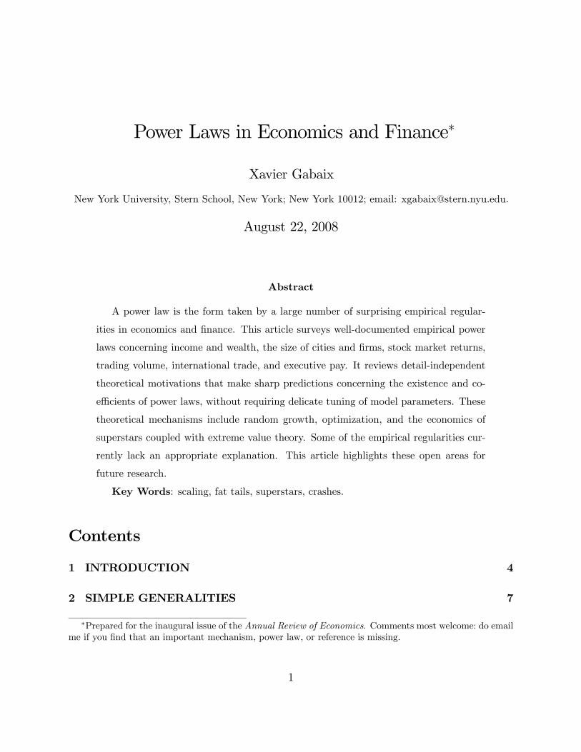
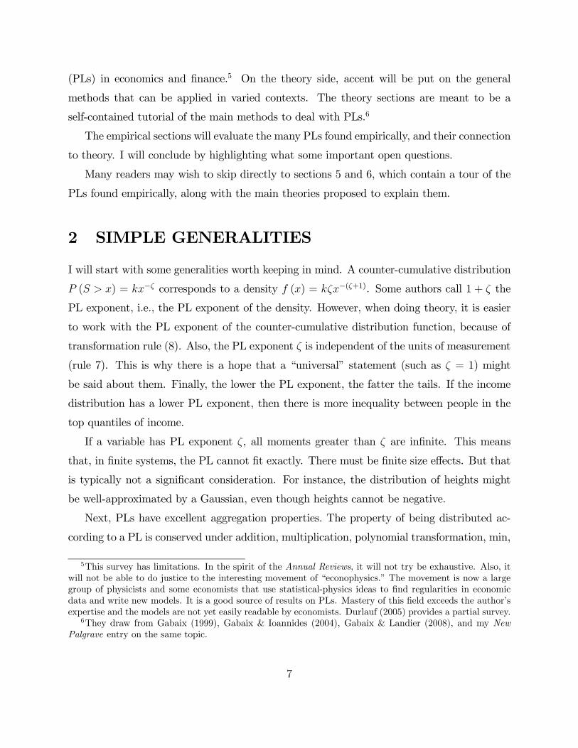
To visualize Zipf’s law, take a country, for instance the United States, and order the
cities3 by population, #1 is New York, #2 is Los Angeles etc. Then, draw a graph; on
the y-axis, place the log of the rank (N.Y. has log rank ln 1, L.A. log rank ln 2), and on
the x-axis, place the log of the population of the corresponding city (which will be called
the “size” of the city). Figure 1 following Krugman (1996) and Gabaix (1999), shows the
resulting plot for the 135 American metropolitan areas listed in the Statistical Abstract of
1Of course, the fit may be only approximate in practice, and may hold only over a bounded range.2G. K. Zipf (1902-1950) was a Harvard linguist (on him, see the 2002 special issue of Glottometrics).
Zipf’s law for cities was first noted by Auerbach (1913), and Zipf’s law for words by Estoup (1916). Ofcourse, G. K. Zipf was needed to explore it in different languages (a painstaking task of tabulation at thetime, with only human computers) and for different countries.
3The term “city” is, strictly speaking, a misnomer; “agglomeration” would be a better term. So for ourpurpose, the “city” of Boston includes Cambridge.
4
00.5
11.5
22.5
33.5
44.5
5
5.50 6.50 7.50 8.50 9.50Log of the Population
Log
of th
e R
ank
Figure 1: Log Size vs Log Rank of the 135 American metropolitan areas listed in the Statis-tical Abstract of the United States for 1991.
the United States for 1991.
We see a straight line, which is rather surprising. There is no tautology causing the data
to automatically generate this shape. Indeed, running a linear regression yields:
lnRank = 10.53− 1.005 lnSize,
(.010) (2)
where the standard deviation of the slope is in parentheses, and the R2 is 0.9864. In accor-
dance with Zipf’s law, when log-rank is plotted against log-size, a line with slope -1.0 (ζ = 1)
appears. This means that the city of rank n has a size proportional to 1/n or terms of the
distribution, the probability that the size of a city is greater than some S is proportional to
1/S: P (Size> S) = a/Sζ, with ζ ' 1. Crucially, Zipf’s law holds pretty well worldwide, aswe will see below.
4We shall see in section 7 that the standard error is too narrow: the proper one is actually1.005 (2/135)
1/2= 0.12, and the regression is better estimated as ln (Rank− 1/2) (then, the estimate is
1.05). But those are details at this stage.
5
Power laws have fascinated economists of successive generations, as expressed, for in-
stance, by the quotation from Schumpeter that opens this article. Champernowne (1953),
Simon (1955), and Mandelbrot (1963) made great strides to achieve Schumpeter’s vision.
And the quest continues. This is what this article will try to cover.
A central question of this review is: What are the robust mechanisms that can explain
this PL? In particular, the goal is not to explain the functional form of the PL, but also why
the exponent should be 1. An explanation should be detail-independent : it should not rely on
the fine balance between transportation costs, demand elasticities and the like, that, as if by
coincidence, conspire to produce an exponent of 1. No “fine-tuning” of parameters is allowed,
except perhaps to say that some “frictions” would be very small. An analogy for detail-
independence is the central limit theorem: if we take a variable of arbitrary distribution, the
normalized mean of successive realizations always has an asymptotically normal distribution,
independently of the characteristic of the initial process. Likewise, whatever the particulars
driving the growth of cities, their economic role etc., we will see that as soon as cities satisfy
Gibrat’s law (see the Glossary) with very small frictions, their population distribution will
converge to Zipf’s law. PLs give the hope of robust, detail-independent economic laws.
Furthermore, PLs can be a way to gain insights into important questions from a fresh
perspective. For instance, consider stock market crashes. Most people would agree that
understanding their origins is interesting question (e.g. for welfare, policy and risk man-
agement). Recent work (reviewed later) has indicated that stock market returns follow a
power law, and furthermore, it seems that stock market crashes are not outliers to the power
law (Gabaix et al. 2005). Hence, a unified economic mechanism might generate not only
the crashes, but actually a whole PL distribution of crash-like events. This can guide theo-
ries, because instead of having a theorize on just a few data points (a rather unconstrained
problem), one has to write a theory of the whole PL of large stock market fluctuations.
Hence thinking about the tail distribution may give us both insights about the “normal-
time” behavior of the market (inside the tails), and also the most extreme events. Trying to
understanding PL might give us the key to understanding stock market crashes.
This article will offer a critical review of the state of theory and empirics for power laws
6
(PLs) in economics and finance.5 On the theory side, accent will be put on the general
methods that can be applied in varied contexts. The theory sections are meant to be a
self-contained tutorial of the main methods to deal with PLs.6
The empirical sections will evaluate the many PLs found empirically, and their connection
to theory. I will conclude by highlighting what some important open questions.
Many readers may wish to skip directly to sections 5 and 6, which contain a tour of the
PLs found empirically, along with the main theories proposed to explain them.
2 SIMPLE GENERALITIES
I will start with some generalities worth keeping in mind. A counter-cumulative distribution
P (S > x) = kx−ζ corresponds to a density f (x) = kζx−(ζ+1). Some authors call 1 + ζ the
PL exponent, i.e., the PL exponent of the density. However, when doing theory, it is easier
to work with the PL exponent of the counter-cumulative distribution function, because of
transformation rule (8). Also, the PL exponent ζ is independent of the units of measurement
(rule 7). This is why there is a hope that a “universal” statement (such as ζ = 1) might
be said about them. Finally, the lower the PL exponent, the fatter the tails. If the income
distribution has a lower PL exponent, then there is more inequality between people in the
top quantiles of income.
If a variable has PL exponent ζ, all moments greater than ζ are infinite. This means
that, in finite systems, the PL cannot fit exactly. There must be finite size effects. But that
is typically not a significant consideration. For instance, the distribution of heights might
be well-approximated by a Gaussian, even though heights cannot be negative.
Next, PLs have excellent aggregation properties. The property of being distributed ac-
cording to a PL is conserved under addition, multiplication, polynomial transformation, min,
5This survey has limitations. In the spirit of the Annual Reviews, it will not try be exhaustive. Also, itwill not be able to do justice to the interesting movement of “econophysics.” The movement is now a largegroup of physicists and some economists that use statistical-physics ideas to find regularities in economicdata and write new models. It is a good source of results on PLs. Mastery of this field exceeds the author’sexpertise and the models are not yet easily readable by economists. Durlauf (2005) provides a partial survey.
6They draw from Gabaix (1999), Gabaix & Ioannides (2004), Gabaix & Landier (2008), and my NewPalgrave entry on the same topic.
7
and max. The general rule is that, when we combine two PL variables, the fattest (i.e., the
one with the smallest exponent) PL dominates. Call ζX the PL exponent of variable X. The
properties above also hold if X is thinner than any PL, i.e. ζx = +∞ and Eh|X|ζ
iis finite
for all positive ζ, for instance if X is a Gaussian.
Indeed, for X1, ..., Xn independent random variables and α a positive constant, we have
the following formulas (see Jessen & Mikosch 2006 for a survey) 7 how PLs beget new PLs
(the “inheritance” mechanism for PLs)
ζX1+···+Xn = min (ζX1, . . . , ζXn) (3)
ζX1·····Xn = min (ζX1, . . . , ζXn) (4)
ζmax(X1,...,Xn) = min (ζX1, . . . , ζXn) (5)
ζmin(X1,...,Xn) = ζX1 + · · ·+ ζXn (6)
ζαX = ζX (7)
ζXα =ζXα. (8)
For instance, if X is a PL variable for ζX < ∞ and Y is PL variable with an exponent
ζY ≥ ζX , then X + Y,X · Y , max (X, Y ) are still PLs with the same exponent ζX . This
property holds when Y is normal, lognormal, or exponential, in which case ζX =∞.Hence,
multiplying by normal variables, adding non-fat tail noise, or summing over i.i.d. variables
preserves the exponent.
These properties make theorizing with PL very streamlined. Also, they give the empiricist
hope that those PLs can be measured, even if the data is noisy. Although noise will affect
statistics such as variances, it will not affect the PL exponent. PL exponents carry over the
“essence” of the phenomenon: smaller order effects do not affect the PL exponent.
Also, the above formulas indicate how to use PLs variables to generate new PLs.
7Several proofs are quite easy. Take (8). If P (X > x) = kx−ζ , then P (Xα > x) = P¡X > x1/α
¢=
kx−ζ/α, so ζXα = ζX/α.
8
3 THEORY I: RANDOM GROWTH
This section provides the a key mechanism that explains economic PLs: proportional random
growth. The next section will explore other mechanisms. Bouchaud (2001), Mitzenmacher
(2003), Sornette (2004), and Newman (2007) survey mechanisms from a physics perspective.
3.1 Basic ideas: Proportional random growth leads to a PL
A central mechanism to explain distributional PLs is proportional random growth. The
process originates in Yule (1925), which was developed in economics by Champernowne
(1953) and Simon (1955), and rigorously studied by Kesten (1973).
Take the example of an economy with a continuum of cities, with mass 1. Call P it the
population of city i and P t the average population size. We define Sit = P i
t /P t, the “normal-
ized” population size. Throughout this paper, we will reason in “normalized” sizes.8 This
way, the average city size remains constant, here at a value 1. Such a normalization is im-
portant in any economic application. As we want to talk about the steady state distribution
of cities (or incomes, etc.), so we need to normalize to ensure such a distribution exists.
Suppose that each city i has a population Sit, that increases by a growth rate γ
it+1from
time t to time t+ 1:
Sit+1 = γit+1S
it (9)
Assume that the γit+1 are identically and independently distributed, with density f (γ),
at least in the upper tail. Call Gt (x) = P (Sit > x), the counter-cumulative distribution
function. The equation of motion of Gt is:
Gt+1 (x) = P¡Sit+1 > x
¢= P
¡Sit > x/γit+1
¢= E
£Gt
¡x/γit+1
¢¤=
Z ∞
0
Gt
µx
γ
¶f (γ) dγ.
8Economist Levy and physicist Solomon (1996) created a resurgent interest for of Champernowne’s ran-dom growth process with lower bound, and, to the best of my knowledge, are the first normalization by theaverage for the them. Wold and Wittle (1957) may be the first to introduce the normalization by a growthfactor in a random growth model.
9
Its steady state distribution G, if it exists, satisfies
G(S) =
Z ∞
0
G
µS
γ
¶f (γ) dγ.
One can try the functional form G(S) = k/Sζ , where k is a constant. Plugging it in gives:
1 =R∞0
γζf (γ) dγ, i.e.
Champernowne’s equation: E£γζ¤= 1. (10)
Hence, if the steady state distribution is Pareto in the upper tail, then the exponent ζ is the
positive root of equation 10 (if such a root exists).
Equation (10) is fundamental in random growth processes. To the best of my knowledge,
it has been first derived by Champernowne in his 1937 doctoral dissertation, and then pub-
lished in Champernowne (1953). (Publication lags in economics were already long.) The
main antecedent to Champernowne, Yule (1925), does not contain it. Hence, I propose to
name (10) “Champernowne’s equation”.9
Champernowne’s equation says that: Suppose you have a random growth process that,
to the leading order, can be written St+1 ∼ γt+1St for large size, where γ is an i.i.d. random
variable. Then, if there is a steady state distribution, it is a PL with exponent ζ, where ζ is
the positive solution of (10). ζ can be related to the distribution of the (normalized) growth
rate γ.
Above we assumed that the steady state distribution exists. To guaranty that existence,
some deviations from a pure random growth process (some “friction”) needs to be added.
Indeed, we didn’t have a friction, we would not get a PL distribution. Indeed, if (9) held
throughout the distribution, then we would have lnSit = lnS
i0+Pt
s=1 ln γit+1, and the distri-
bution would be lognormal, without a steady state (as var (lnSit) = var (lnSi
0)+var (ln γ) t,
the variance growth without bound). This is Gibrat’s (1931) observation. Hence, to make
sure that the steady state distribution exists, one needs some friction that prevents from
9Champernowne also (like Simon) programmed chess-playing computers (with Alan Turing), and invented“Champernowne’s number”, which consists of a decimal fraction in which the decimal integers are writtensucessively: .01234567891011121314...99100101... It is apparently interesting in computer science as it seems“random” to most tests.
10
cities or firms from becoming too small. Mechanically, potential frictions a positive constant
added in (9) that that prevents small entities from becoming too small (section 3.3), .a lower
bound for sizes, with “reflecting barrier” (section 3.4), e.g. a small death rate of cities or
firms. Economically, those forces might a death rate, or a fixed cost that prevents very small
firms from operating, or even very cheap rents for small cities. This is what the later sections
will detail. Importantly, the particular force that happens for small sizes typically does not
affect the PL exponent in the upper tail: in equation (10), only the growth rate in the upper
tail matters.
The above random growth process also can explain the Pareto distribution of wealth,
interpreting Sit as the wealth of individual i.
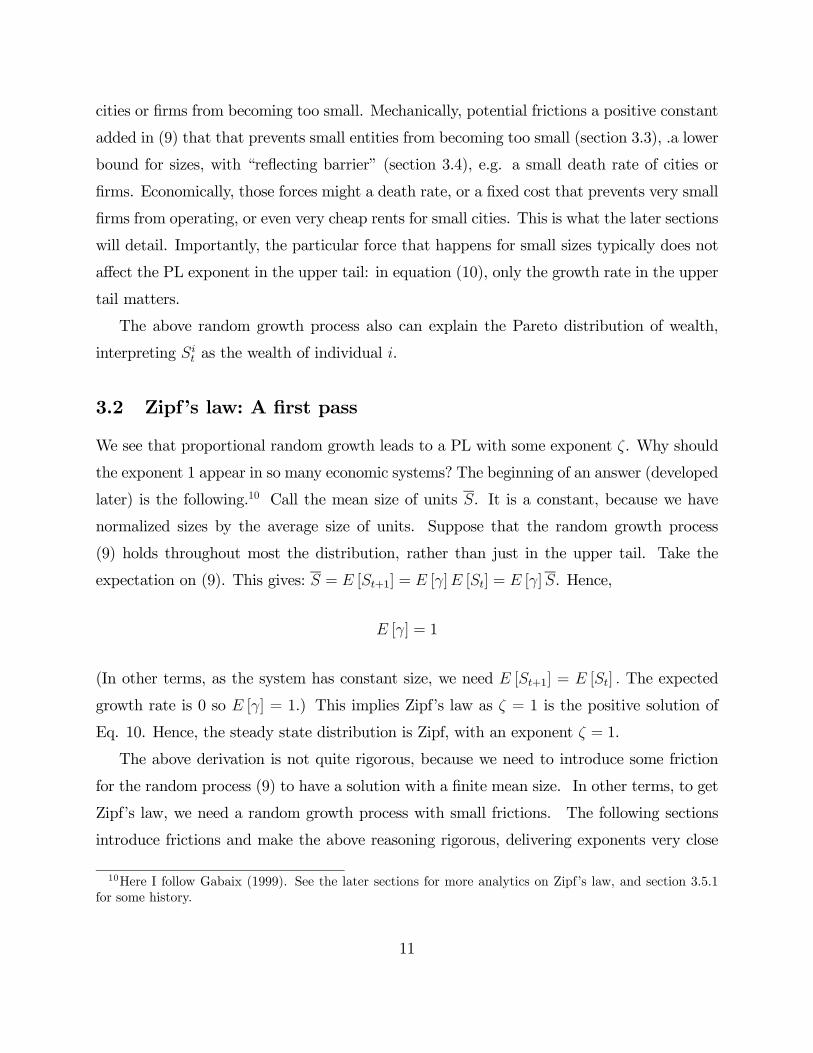
3.2 Zipf’s law: A first pass
We see that proportional random growth leads to a PL with some exponent ζ. Why should
the exponent 1 appear in so many economic systems? The beginning of an answer (developed
later) is the following.10 Call the mean size of units S. It is a constant, because we have
normalized sizes by the average size of units. Suppose that the random growth process
(9) holds throughout most the distribution, rather than just in the upper tail. Take the
expectation on (9). This gives: S = E [St+1] = E [γ]E [St] = E [γ]S. Hence,
E [γ] = 1
(In other terms, as the system has constant size, we need E [St+1] = E [St] . The expected
growth rate is 0 so E [γ] = 1.) This implies Zipf’s law as ζ = 1 is the positive solution of
Eq. 10. Hence, the steady state distribution is Zipf, with an exponent ζ = 1.
The above derivation is not quite rigorous, because we need to introduce some friction
for the random process (9) to have a solution with a finite mean size. In other terms, to get
Zipf’s law, we need a random growth process with small frictions. The following sections
introduce frictions and make the above reasoning rigorous, delivering exponents very close
10Here I follow Gabaix (1999). See the later sections for more analytics on Zipf’s law, and section 3.5.1for some history.
11
to 1.
When frictions are large (e.g. with reflecting barrier or the Kesten process in Gabaix,
Appendix 1), a PL will arise but Zipf’s law will not hold exactly. In those cases, small units
grow faster than large units. Then, the normalized mean growth rate of large cities is less
than 0, i.e. E [γ] < 1, which implies ζ > 1. In sum, the proportional random growth with
frictions leads to PL and proportional random growth with small frictions leads to a special
type of PL, Zipf’s law.
3.3 Rigorous approach via Kesten processes
One case where random growth processes have been completely rigorously treated are the
“Kesten processes”. Consider the process St = AtSt−1+Bt, where (At, Bt) are i.i.d. random
variables. Note that if St has a steady state distribution, then the distribution of St and
ASt + B are the same, something we can write S =d AS + B. The basic formal result is
from Kesten (1973), and was extended by Verwaat (1979) and Goldie (1991).
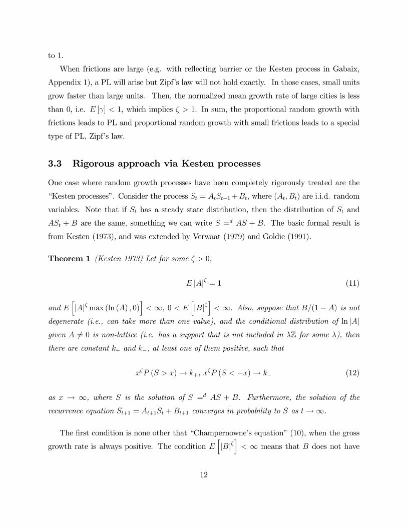
Theorem 1 (Kesten 1973) Let for some ζ > 0,
E |A|ζ = 1 (11)
and Eh|A|ζ max (ln (A) , 0)
i<∞, 0 < E
h|B|ζ
i<∞. Also, suppose that B/(1− A) is not
degenerate (i.e., can take more than one value), and the conditional distribution of ln |A|given A 6= 0 is non-lattice (i.e. has a support that is not included in λZ for some λ), then
there are constant k+ and k−, at least one of them positive, such that
xζP (S > x)→ k+, xζP (S < −x)→ k− (12)
as x → ∞, where S is the solution of S =d AS + B. Furthermore, the solution of the
recurrence equation St+1 = At+1St +Bt+1 converges in probability to S as t→∞.
The first condition is none other that “Champernowne’s equation” (10), when the gross
growth rate is always positive. The condition Eh|B|ζ
i< ∞ means that B does not have
12
fatter tails than a PL with exponent ζ (otherwise, the PL exponent of S would presumably
be that of B).
Kesten’s theorem formalizes the heuristic reasoning of section 2.2. However, that same
heuristic logic makes it clear that a more general process will still have the same asymptotic
distribution. For instance, one may conjecture that the process St = AtSt−1 + φ (St−1, Bt),
with φ (S,Bt) = o (S) for large x should have an asymptotic PL tail in the sense of (12),
with the same exponent ζ. Such a result does not seem to have been proven yet.
To illustrate the power of the Kesten framework, let us examine an application to ARCH
processes.
Application: ARCH processes have PL tails Consider an ARCH process: σ2t =
ασ2t−1ε2t + β, and the return is εtσt−1, with εt independent of σt−1. Then, we are in the
framework of Kesten’s theory, with St = σ2t , At = αε2t , and Bt = β. Hence, squared
volatility σ2t follows a PL distribution with exponent ζ such that Eh¡αε2t+1
¢ζi= 1. By the
rules (8), that will mean ζσ = 2ζ. As Ehε2ζt+1
i< 1, ζε ≥ 2ζ, and rule (4) implies that returns
will follow a PL, ζr = min (ζσ, ζe) = 2ζ. The same reasoning would show that GARCH
processes have PL tails.
3.4 Continuous-Time approach
This subsection is more technical, and the reader may wish to skip to the next section. The
benefit, as always, is that continuous-time makes calculations easier.
3.4.1 Basic tools, and random growth with reflected barriers
Consider the continuous time process:
dXt = μ (Xt, t) dt+ σ (Xt, t) dzt
where zt is a Brownian motion. The process Xt could be reflected at some points. Call
f (x, t) the distribution at time t. To describe the evolution of the distribution, given initial
13
conditions f (x, t = 0), the basic tool is the Forward Kolmogorov equation:
∂tf (x, t) = −∂x [μ (x, t) f (x, t)] + ∂xx
∙σ2 (x, t)
2f (x, t)
¸(13)
where ∂tf = ∂f/∂t, ∂xf = ∂f/∂x and ∂xxf = ∂2f/∂x2. Its major application is to calculate
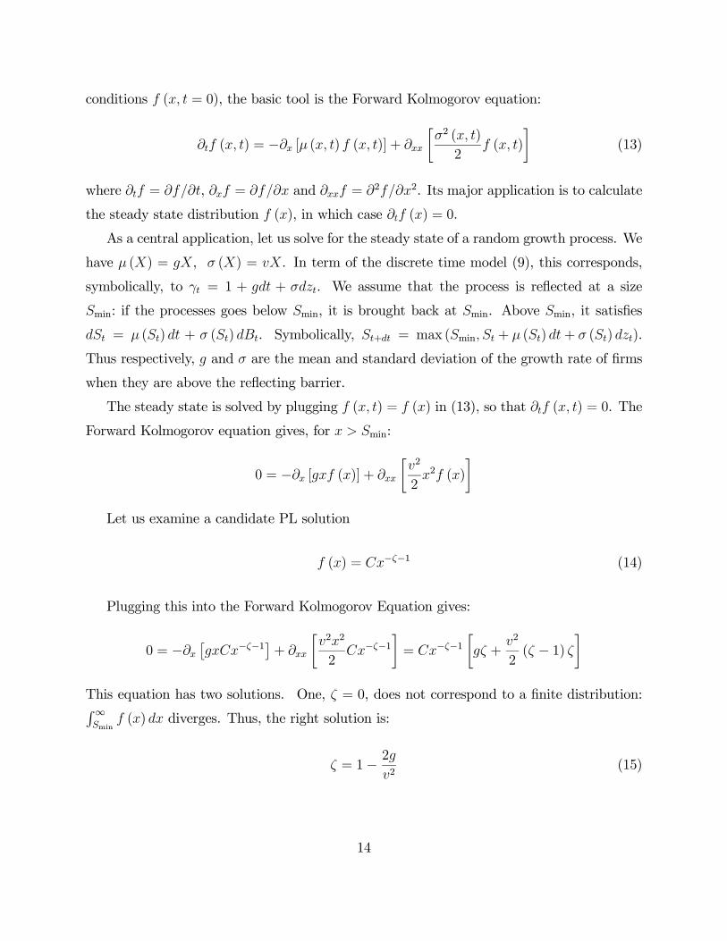
the steady state distribution f (x), in which case ∂tf (x) = 0.
As a central application, let us solve for the steady state of a random growth process. We
have μ (X) = gX, σ (X) = vX. In term of the discrete time model (9), this corresponds,
symbolically, to γt = 1 + gdt + σdzt. We assume that the process is reflected at a size
Smin: if the processes goes below Smin, it is brought back at Smin. Above Smin, it satisfies
dSt = μ (St) dt + σ (St) dBt. Symbolically, St+dt = max (Smin, St + μ (St) dt+ σ (St) dzt).
Thus respectively, g and σ are the mean and standard deviation of the growth rate of firms
when they are above the reflecting barrier.
The steady state is solved by plugging f (x, t) = f (x) in (13), so that ∂tf (x, t) = 0. The
Forward Kolmogorov equation gives, for x > Smin:
0 = −∂x [gxf (x)] + ∂xx
∙v2
2x2f (x)
¸Let us examine a candidate PL solution
f (x) = Cx−ζ−1 (14)
Plugging this into the Forward Kolmogorov Equation gives:
0 = −∂x£gxCx−ζ−1
¤+ ∂xx
∙v2x2
2Cx−ζ−1
¸= Cx−ζ−1
∙gζ +
v2
2(ζ − 1) ζ
¸This equation has two solutions. One, ζ = 0, does not correspond to a finite distribution:R∞Smin
f (x) dx diverges. Thus, the right solution is:
ζ = 1− 2gv2
(15)
14
Eq. (15) gives us the PL exponent of the distribution.11 Note that, for the mean of the
process to be finite, we need ζ > 1, hence g < 0. That makes sense. As the total growth
rate of the normalized population is 0 and the growth rate of reflected units is necessarily
positive, the growth rate of non-reflected units (g) must be negative.
Using economic arguments that the distribution has to go smoothly to 0 for large x, one
can show that (14) is the only solution. Ensuring that the distribution integrates to a mass
1 gives the constant C and the distribution: f (x) = ζx−ζ−1Sζmin then:
P (S > x) =
µx
Smin
¶−ζ(16)
Hence, we have seen that random growth with a reflecting lower barrier generates a
Pareto — an insight in Champernowne (1953).
Why would Zipf’s law hold then? Note that the mean size is:
S =
Z ∞
Smin
xf (x) dx =
Z ∞
Smin
x · ζx−ζ−1Sζmindx = ζSζ
min
∙x−ζ+1
−ζ + 1
¸∞Smin
=ζ
ζ − 1Smin
Thus, we see that the Zipf exponent is:
ζ =1
1− Smin/S. (17)
We find again a reason for Zipf’s law: when the zone of “frictions” is very small (Smin/S
small), then the PL exponent goes to 1. When frictions are very small, the steady state
distribution approaches Zipf’s law. But, of course, it can never exactly be at Zipf’s law: in
(17), the exponent is always above 1.
This model ensures that, given a minimum size Smin, average size S, and a volatility
v, the mean growth rate g of the cities that are not reflected will self-organize, so as to
satisfy (15) and (17). Zipf’s law arises because the fraction of the population that is in the
“reflected” region itself is endogenous.
11This also comes heuristically also from eq. 10, applied to γt = 1 + gdt + σdzt, and by Ito’s lemma
1 = Ehγζt
i= 1 + ζgdt+ ζ (ζ − 1) v2/2dt.
15
Another way to “stabilize” the process, so that it has a steady state distribution, is to
have a small death rate. This is to what we next turn.
3.4.2 Extensions with birth, death and jumps
Birth and Death We enrich the process with death and birth. We assume that one
unit of size x dies with Poisson probability δ (x, t) per unit of time dt. We assume that a
quantity j (x, t) of new units is born at size x. Call n (x, t) dx the number of units with size
in [x, x+ dx). The Forward Kolmogorov Equation describes its evolution as:
∂tn (x, t) = −∂x [μ (x, t)n (x, t)] + ∂xx
∙σ2 (x, t)
2n (x, t)
¸− δ (x, t)n (x, t) + j (x, t) (18)
Application: Zipf’s law with death and birth of cities rather than a lower
barrier As an application, consider a random growth law model where existing units grow
at rate g and have volatility σ. Units die with a Poisson rate δ, and are immediately
“reborn” at a size S∗. There is no reflecting barrier: instead, the death and rebirth processes
generate the stability of the steady state distribution. (See also Malevergne et al. 2008).
For simplicity, we assume a constant size for the system: the number of units is constant.
The Forward Kolmogorov Equation (outside the point of reinjection S∗), evaluated at the
steady state distribution f (x), is:
0 = −∂x [gxf (x)] + ∂xx
∙v2x2
2f (x)
¸− δf (x)
We look for elementary solutions of the form f (x) = Cx−ζ−1. Plugging this into the above
equation gives:
0 = −∂x£gxx−ζ−1
¤+ ∂xx
∙v2x2
2x−ζ−1
¸− δx−ζ−1
i.e.
0 = ζg +v2
2ζ (ζ − 1)− δ (19)
This equation now has a negative root ζ−, and a positive root ζ+. The general solution
16
for x different from S∗ is f (x) = C−x−ζ−−1+C+x
−ζ+−1. Because units are reinjected at size,
S∗ the density f could be at that value. The steady-state distribution is:12
f (x) =
⎧⎨⎩ C (x/S∗)−ζ−−1 for x < S∗
C (x/S∗)−ζ+−1 for x > S∗
and the constant is C = −ζ+ζ−/ (ζ+ − ζ−). This is the “double Pareto” (Champernowne
1953, Reed 2001).
We can study how Zipf’s law arises from such a system. The mean size of the system is:
S = S∗ζ+ζ−
(ζ+ − 1) (1− ζ−)(20)
As (19) implies that ζ+ζ− = −2δ/σ2, this equation can be rearranged at:
(ζ+ − 1)µ1 +
2δ/σ2
ζ+
¶=
S∗
S2δ/σ2
Hence, we obtain Zipf’s law (ζ+ → 1) if either (i) S∗S→ 0 (reinjection is done at very
small sizes), or (ii) δ → 0 (the death rate is very small). We see again that Zipf’s law arises
when there is random growth in most of the distribution, and frictions are very small.
Jumps As another enhancement, consider jumps: with some probability pdt, a jump oc-
curs, the process size is multiplied by eGt, which is stochastic and i.i.d. Xt+dt =³1 + μdt+ σdzt + eGtdJt
´Xt
where dJt is a jump process: dJt = 0 with probability 1− pdt and dJt = 1 with probability
pdt.
This corresponds to a “death” rate δ (x, t) = p, and an injection rate j (x, t) = pE [n (x/G, t) /G].
The latter comes from the fact that that injection as a size above x come from a size above
x/G. Hence, using (18), the Forward Kolmogorov Equation is:
∂tn (x, t) = −∂x [μ (x, t)n (x, t)] + ∂xx
∙σ2 (x, t)
2n (x, t)
¸+ pE
∙n (x/G, t)
G− n (x, t)
¸(21)
12For x > S∗, we need the solution to be integrable when x→∞: that imposes C− = 0. For x < S∗, weneed the solution to be integrable when x→ 0: that imposes C+ = 0.
17
where the last expectation is taken over the realizations of G.
Application: Impact of death and birth in the PL exponent Combining (18)
and (21), the Forward Kolmogorov Equation is:
∂tn (x, t) = −∂x [μ (x, t)n (x, t)]+∂xx∙σ2 (x, t)
2n (x, t)
¸−δ (x, t)n (x, t)+j (x, t)+pE
∙n (x/G, t)
G− n (x, t)
¸(22)
It features the impact of mean growth (μ term), volatility (σ), birth (j), death (δ), jumps
(G).
For instance, take random growth with μ (x) = g∗x, σ (x) = σ∗x, death rate δ, and
birth rate ν, and applying this to a steady state distribution n (x, t) = f (x). Plugging
f (x) = f (0)x−ζ−1 into (22) gives:
0 = −δx−ζ−1 + νx−ζ−1 − ∂x¡g∗x
−ζ¢+ ∂xx
µσ∗x
2
2x−ζ−1
¶+E
∙³ xG
´−ζ−1 1G− 1¸
i.e.
0 = −δ + ν + g∗ζ +σ2∗2ζ (ζ − 1) + pE
£Gζ − 1
¤(23)
We see that the PL exponent ζ is lower (the distribution has fatter tails) when the growth
rate is higher, the death rate is lower, the birth rate is higher, and the variance is higher (in
the domain ζ > 1). All those forces make it easier to obtain large firms in the steady state
distribution.
3.4.3 Deviations from a power law
Recognizing the possibility that Gibrat’s Law might not hold exactly, Gabaix (1999) also
examines the case where cities grow randomly with expected growth rates and standard
deviations that depend on their sizes. That is, the (normalized) size of city i at time t varies
according to:dStSt
= g(St)dt+ v(St)dzt, (24)
where g(S) and v2(S) denote, respectively, the instantaneous mean and variance of the
growth rate of a size S city, and zt is a standard Brownian motion. In this case, the
18
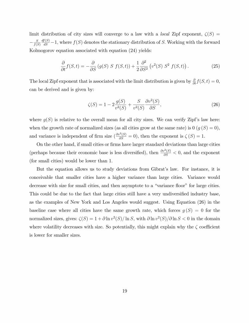
limit distribution of city sizes will converge to a law with a local Zipf exponent, ζ(S) =
− Sf(S)
df(S)dS−1, where f(S) denotes the stationary distribution of S.Working with the forward
Kolmogorov equation associated with equation (24) yields:
∂
∂tf(S, t) = − ∂
∂S(g(S) S f(S, t)) +
1
2
∂2
∂S2¡v2(S) S2 f(S, t)
¢. (25)
The local Zipf exponent that is associated with the limit distribution is given by ∂∂tf(S, t) = 0,
can be derived and is given by:
ζ(S) = 1− 2 g(S)v2(S)
+S
v2(S)
∂v2(S)
∂S, (26)
where g(S) is relative to the overall mean for all city sizes. We can verify Zipf’s law here:
when the growth rate of normalized sizes (as all cities grow at the same rate) is 0 (g (S) = 0),
and variance is independent of firm size (∂v2(S)∂S
= 0), then the exponent is ζ (S) = 1.
On the other hand, if small cities or firms have larger standard deviations than large cities
(perhaps because their economic base is less diversified), then ∂v2(S)∂S
< 0, and the exponent
(for small cities) would be lower than 1.
But the equation allows us to study deviations from Gibrat’s law. For instance, it is
conceivable that smaller cities have a higher variance than large cities. Variance would
decrease with size for small cities, and then asymptote to a “variance floor” for large cities.
This could be due to the fact that large cities still have a very undiversified industry base,
as the examples of New York and Los Angeles would suggest. Using Equation (26) in the
baseline case where all cities have the same growth rate, which forces g (S) = 0 for the
normalized sizes, gives: ζ(S) = 1+ ∂ ln v2(S)/ lnS, with ∂ ln v2(S)/∂ lnS < 0 in the domain
where volatility decreases with size. So potentially, this might explain why the ζ coefficient
is lower for smaller sizes.
19
3.5 Complements on Random Growth
3.5.1 Simon’s and other models
This may be a good time to talk about some other random growth models. The simplest is
a model by Steindl (1965). New cities are born at a rate ν, and with a constant initial size,
and existing cities grow at a rate γ. The result is that the distribution of new cities will be
in the form of a PL, with an exponent ζ = ν/γ, as a quick derivation shows13. However,
this is quite problematic as an explanation for Zipf’s law. It delivers the result we want,
namely the exponent of 1, only by assuming that historically ν = γ. This is quite implausible
empirically, especially for mature urban systems, for which it is very likely that ν < γ.
Steindl’s model gives us a simple way to understand Simon’s (1955) model (for a particu-
larly clear exposition of Simon’s model, see Krugman 1996, and Yule 1925 for an antecedent).
New migrants (of mass 1, say) arrive at each period. With probability π, they form a new
city, whilst with probability 1− π they go to an existing city. When moving to an existing
city, the probability that they choose a given city is proportional to its population.
This model generates a PL, with exponent ζ = 1/(1 − π). Thus, the exponent of 1
has a very natural explanation: the probability π of new cities is small. This seems quite
successful. And indeed, this makes Simon’s model an important, first explanation of Zipf’s
law via small frictions. However, Simon’s model suffers from two large drawbacks that do
not allow it to be a acceptable solution for Zipf’s law.14
First, Simon’s model has the same problem as Steindl’s model (Gabaix, 1999, Appendix
3). If the total population growth rate is γ0, Simon’s model generates a growth rate in the
number of cities equal to ν = γ0, and a growth rate of existing cities equal to γ = (1− π) γ0.
Hence, Simon’s model implies that the rate of growth of the number of cities has to be
greater than the rate of growth of the population of the existing cities. This essential model
feature is empirically quite unlikely15.
13The cities of size greater than S are the cities of age greater than a = lnS/γ. Because of the form ofthe birth process, the number of these cities is proportional to e−νa = e−ν lnS/γ = S−ν/γ , which gives theexponent ζ = ν/γ.14Krugman (1996) also mentions that Simon’s model may converge too slowly compared to historical
time-scales.15This can be fixed by assuming the the “birth size” of a city grows at a positive rate. But then the model
20
Second, the model predicts that the variance of the growth rate of an existing unit of size
S should be σ2 (S) = k/S. (Indeed, in Simon’s model a unit of size S receives, metaphorically
speaking, a number of independent arrival shocks proportional to S). Larger units have a
much smaller standard deviation of growth rate than small cities. Such a strong departure
from Gibrat’s law for variance is almost certainly not true, for cities (Ioannides & Overman
2003) or firms (Stanley et al. 1996).
This violation of Gibrat’s law for variances with Simon’s model seems to have been
overlooked in the literature. Simon’s model has enjoyed a great renewal in the literature on
the evolution of web sites (Barabasi & Albert 1999). Hence it seems useful to test Gibrat’s
law for variance in the context of web site evolution and accordingly correct the model.
Till the late 1990s, the central argument for an exponent of 1 for the Pareto was still
Simon (1955). Other models (e.g. surveyed in Carroll 1982 and Krugman 2006) have no
clear economic meaning (like entropy maximization) or do not explain why the exponent
should be 1. Then two independent literatures, in physics and economics, entered the fray.
Levy & Solomon (1996) was an influential impulse on power laws, that addresses the
Zipf case at most elliptically; however, Malcai et al. (1999) do spell out a mechanism for
Zipf’s law. Marsili & Zhang’s (1998) model can be tuned to yield Zipf’s law, but that tuning
implies that gross flow in and out of a city is proportional to the city size squared (rather than
linear in it), which is most likely counterfactually huge for large cities. Zanette & Manrubia
(1997, 1998) andMarsili et al. (1998b) present arguments for Zipf’s law (see also Marsili et al.
1998a, and on the following page Z&M’s reply). Z&M postulate a growth process γt that can
take only two values, and insist on the analogy with the physics of intermittency. Marsili et
al. analyze a rich portfolio choice problem, and highlight the analogy with polymer physics.
As a result, their interesting works may not elucidate the generality of the mechanism for
Zipf’s law outlined in section 3.2.
In economics, Krugman (1996) revived the interest for Zipf’s law. He surveys existing
mechanisms, finds them insufficient, and proposes that Zipf’s law may come from a power
law of natural advantages, perhaps via percolation. But the origin of the exponent of 1 is
not explained. Gabaix (1999), written independently of those physics papers, identifies the
is quite different, and the next problem remains.
21
mechanism outlined in section 3.2, establishes when the Zipf limit obtains in a quite general
way (with Kesten processes, and with the reflecting barrier), provides a baseline economic
model with constant returns to scale, and derives analytically the deviations from Zipf’s law
via deviations from Gibrat’s law. Afterwards, a number of papers (cited elsewhere in this
review) worked out more and more economic models for Gibrat’s law and/or Zipf’s law.
3.5.2 Finite number of units
The above arguments are simple to make when there is a continuum number of cities or
firms. If there is a finite number, the situation is more complicated, as one cannot directly
use the law of large numbers. Malcai et al. (1999) study this case. They note if distribution
has support [Smin, Smax], and the Pareto form f (x) = kx−ζ−1 and there are N cities with
average size S =Rxf (x) dx/
Rf (x) dx, then necessarily:
1 =ζ − 1ζ
1− (Smin/Smax)ζ
1− (Smin/Smax)ζ−1S
Smin(27)
and this formula gives the Pareto exponent ζ. Malcai et al. actually write this formula for
Smax = NS, though one may prefer another choice, the logically maximum size Smax = NS−(N − 1)Smin. For very large number of citiesN and Smax →∞, and a fixed Smin/S, that givesthe simpler formula (17). However, for a finite N , we do not have such a simple formula, and
ζ will not tend to 1 as Smin/S → 0. In other terms, the limits ζ¡N,Smin/S, Smax
¡N,S, Smin
¢¢for N →∞ and Smin/S → 0 do not commute. Malcai et al. make the case that in a variety
of systems, this finite N correction can be important. In any case, this reinforces the feeling
that it would be nice to elucidate the economic nature of the “friction” that prevents small
cities form becoming too small. This way, the economic relation between N , the minimum,
maximum and average size of a firm would be more economically pinned down.
22
4 THEORY II: OTHER MECHANISMS YIELDING
POWER LAWS
We first start with two “economic” ways to obtain PLs: optimization and “superstars” PL
models.
4.1 Matching and power law superstars effects
Let us next see a purely economic mechanism that generates PL to generate PLs is in
matching (possibly bounded) talent with large firms or large audience — the economics of
superstars (Rosen 1982). While Rosen’s model is qualitative, a calculable model is provided
by Gabaix & Landier (2008), whose treatment we follow here. That paper studies the market
for chief executive officers (CEOs).
Firm n ∈ [0, N ] has size S (n) and manager m ∈ [0, N ] has talent T (m). As explainedlater, size can be interpreted as earnings or market capitalization. Low n denotes a larger
firm and low m a more talented manager: S0 (n) < 0, T 0 (m) < 0. In equilibrium, a manager
with talent index m receives total compensation of w (m). There is a mass n of managers
and firms in interval [0, n], so that n can be understood as the rank of the manager, or a
number proportional to it, such as its quantile of rank. The firm number n wants to pick
an executive with talent m, that maximizes firm value due to CEO impact, CS (n)γ T (m),
minus CEO wage, w (m):
maxm
S (n) + CS (n)γ T (m)− w (m) (28)
If γ = 1, CEO impact exhibits constant returns to scale with respect to firm size.
Eq. 28 gives CS (n)γ T 0 (m) = w0 (m). As in equilibrium there is associative matching:
m = n,
w0 (n) = CS (n)γ T 0 (n) , (29)
i.e. the marginal cost of a slightly better CEO, w0 (n), is equal to the marginal benefit of
that slightly better CEO, CS (n)γ T 0 (n). Equation (29) is a classic assignment equation
(Sattinger 1993, Tervio 2008).
23
Specific functional forms are required to proceed further. We assume a Pareto firm size
distribution with exponent 1/α: (we saw a Zipf’s law with α ' 1 is a good fit)
S (n) = An−α (30)
Proposition 1 will show that, using arguments from extreme value theory, there exist
some constants β and B such that the following equation holds for the link between talent
and rank in the upper tail:
T 0 (x) = −Bxβ−1, (31)
This is the key argument that allows Gabaix & Landier (2008) to go beyond antecedent such
as Rosen (1981) and Tervio (2008).
Using functional form (31), we can now solve for CEO wages. Normalizing the reservation
wage of the least talented CEO (n = N) to 0, Equations 29, 30 and 31 imply:
w (n) =
Z N
n
AγBCu−αγ+β−1du =AγBC
αγ − β
£n−(αγ−β) −N−(αγ−β)¤ (32)
In what follows, we focus on the case αγ > β, for which wages can be very large, and consider
the domain of very large firms, i.e., take the limit n/N → 0. In Eq. 32, if the term n−(αγ−β)
becomes very large compared to N−(αγ−β) and w (N):
w (n) =AγBC
αγ − βn−(αγ−β), (33)
A Rosen (1981) “superstar” effect holds. If β > 0, the talent distribution has an upper
bound, but wages are unbounded as the best managers are paired with the largest firms,
which makes their talent very valuable and gives them a high level of compensation.
To interpret Eq. 33, we consider a reference firm, for instance firm number 250 — the
median firm in the universe of the top 500 firms. Call its index n∗, and its size S(n∗). We
obtain that in equilibrium, for large firms (small n), the manager of index n runs a firm of
24
size S (n), and is paid:16
w (n) = D (n∗)S(n∗)β/αS (n)γ−β/α (34)
where S(n∗) is the size of the reference firm and D (n∗) =−Cn∗T 0(n∗)
αγ−β is independent of the
firm’s size.
We see how matching creates a “dual scaling equation” (34), or double PL, which has
three implications:
(a) Cross-sectional prediction. In a given year, the compensation of a CEO is proportional
to the size of his firm size to the power γ − β/α, S(n)γ−β/α
(b) Time-series prediction. When the size of all large firms is multiplied by λ (perhaps
over a decade), the compensation at all large firms is multiplied by λγ. In particular, the
pay at the reference firm is proportional to S(n∗)γ.
(c) Cross-country prediction. Suppose that CEO labor markets are national rather than
integrated. For a given firm size S, CEO compensation varies across countries, with the
market capitalization of the reference firm, S(n∗)β/α, using the same rank n∗ of the reference
firm across countries.
Section 5.5 presents much evidence for prediction (a), the “Roberts’ law in the cross-
section of CEO pay. Gabaix & Landier (2008) presents evidence supporting in particular (b)
and (c), for the recent period at least.
The methodological moral for this section is that (34) exemplifies a purely economic
mechanism that generates PLs: matching, combined with extreme value theory for the initial
units (e.g. firm sizes) and the spacings between talents. Fairly general conditions yield a
dual scaling relation (34).
16The proof is thus. As S = An−α, S(n∗) = An−α∗ , n∗T 0 (n∗) = −Bnβ∗ , we can rewrite Eq. 33,
(αγ − β)w (n) = AγBCn−(αγ−β) = CBnβ∗ ·¡An−α∗
¢β/α · ¡An−α¢(γ−β/α)= −Cn∗T 0 (n∗)S(n∗)β/αS (n)γ−β/α
25
4.2 Extreme Value Theory and Spacings of Extremes in the Upper
Tail
We now develop the point mentioned in the previous section: Extreme value theory shows
that, for all “regular” continuous distributions, a large class that includes all standard distri-
butions, the spacings between extremes is approximately (31). The importance of this point
in economics seems to have been seen first by Gabaix & Landier (2008), whose treatment
we follow here. The following two definitions specify the key concepts.
Definition 1 A function L defined in a right neighborhood of 0 is slowly varying if: ∀u > 0,
limx↓0 L (ux) /L (x) = 1.
Prototypical examples include L (x) = a or L (x) = a ln 1/x for a constant a. If L is
slowly varying, it varies more slowly than any PL xε, for any non-zero ε.
Definition 2 The cumulative distribution function F is regular if its associated density f =
F 0 is differentiable in a neighborhood of the upper bound of its support, M ∈ R∪{+∞}, andthe following tail index ξ of distribution F exists and is finite:
ξ = limt→M
d
dt
1− F (t)
f (t). (35)
Embrechts et al. (1997, p.153-7) show that the following distributions are regular in the
sense of Definition 2: uniform (ξ = −1), Weibull (ξ < 0), Pareto, Fréchet (ξ > 0 for both),Gaussian, lognormal, Gumbel, lognormal, exponential, stretched exponential, and loggamma
(ξ = 0 for all).
This means that essentially all continuous distributions usually used in economics are
regular. In what follows, we denote F (t) = 1−F (t) . ξ indexes the fatness of the distribution,with a higher ξ meaning a fatter tail.17
17ξ < 0 means that the distribution’s support has a finite upper boundM , and for t in a left neighborhoodof M , the distribution behaves as F (t) ∼ (M − t)−1/ξ L (M − t). This is the case that will turn out to berelevant for CEO distributions. ξ > 0 means that the distribution is “in the domain of attraction” of theFréchet distribution, i.e. behaves similar to a Pareto: F (t) ∼ t−1/ξL (1/t) for t→∞. Finally ξ = 0 meansthat the distribution is in the domain of attraction of the Gumbel. This includes the Gaussian, exponential,lognormal and Gumbel distributions.
26
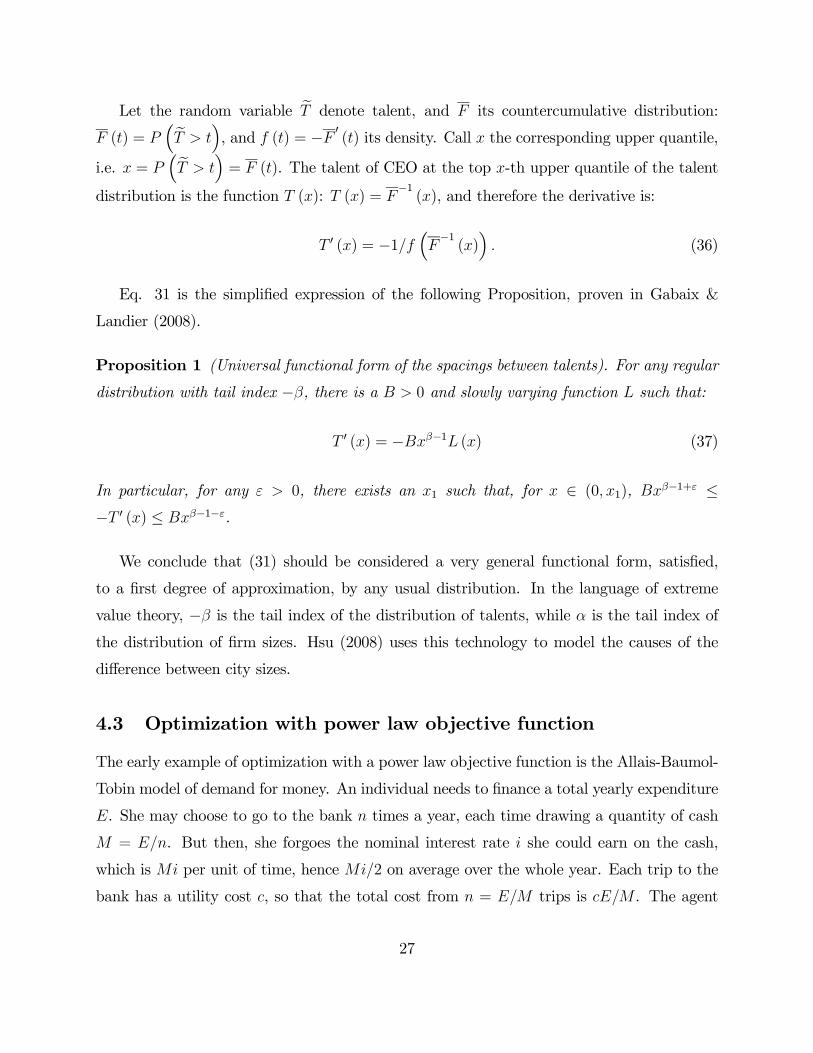
Let the random variable eT denote talent, and F its countercumulative distribution:
F (t) = P³eT > t
´, and f (t) = −F 0
(t) its density. Call x the corresponding upper quantile,
i.e. x = P³eT > t
´= F (t). The talent of CEO at the top x-th upper quantile of the talent
distribution is the function T (x): T (x) = F−1(x), and therefore the derivative is:
T 0 (x) = −1/f³F−1(x)´. (36)
Eq. 31 is the simplified expression of the following Proposition, proven in Gabaix &
Landier (2008).
Proposition 1 (Universal functional form of the spacings between talents). For any regular
distribution with tail index −β, there is a B > 0 and slowly varying function L such that:
T 0 (x) = −Bxβ−1L (x) (37)
In particular, for any ε > 0, there exists an x1 such that, for x ∈ (0, x1), Bxβ−1+ε ≤−T 0 (x) ≤ Bxβ−1−ε.
We conclude that (31) should be considered a very general functional form, satisfied,
to a first degree of approximation, by any usual distribution. In the language of extreme
value theory, −β is the tail index of the distribution of talents, while α is the tail index ofthe distribution of firm sizes. Hsu (2008) uses this technology to model the causes of the
difference between city sizes.
4.3 Optimization with power law objective function
The early example of optimization with a power law objective function is the Allais-Baumol-
Tobin model of demand for money. An individual needs to finance a total yearly expenditure
E. She may choose to go to the bank n times a year, each time drawing a quantity of cash
M = E/n. But then, she forgoes the nominal interest rate i she could earn on the cash,
which is Mi per unit of time, hence Mi/2 on average over the whole year. Each trip to the
bank has a utility cost c, so that the total cost from n = E/M trips is cE/M . The agent
27
minimizes total loss: minM Mi/2 + cE/M . Thus:
M =
r2cE
i.
The demand for cash, M , is proportional to the nominal interest rate to the power −1/2, anice sharp prediction given the simplicity of the model.
In the above mechanism, both the cost and benefits were PL functions of the choice
variable, so that the equilibrium relations are also PL. As we saw in section 3.1, beginning a
theory with a power law yields a final relationship power law. Such a mechanism has been
generalized to other settings, for instance the optimal quantity of regulation (Mulligan &
Shleifer 2004) or optimal trading in illiquid markets (Gabaix et al. 2003, 2006).
4.4 The importance of scaling considerations to infer functional
forms in the utility function
Scaling reasonings are important in macroeconomics. Suppose that you’re looking for a
utility functionP∞
t=0 δtu (ct), that generates a constant interest rate r in an economy that
has constant growth, i.e. ct = c0egt. The Euler equation is 1 = (1 + r) δu0 (ct+1) /u
0 (ct), so we
need u0 (ceg) /u0 (c) to be constant for all c. If we take that the constancy must hold for small g
(e.g. because we talk about small periods), then as u0 (ceg) /u0 (c) = 1+gu00 (c) c/u0 (c)+o (g),
we get u00 (c) c/u0 (c) is a constant, which indeed means that u0 (c) = Ac−γ for some constant
A. This means that, up to an affine transformation, u is in the Constant Relative Risk
Aversion Class (CRRA): u (c) = (c1−γ − 1) / (1− γ) for γ 6= 1, or u (c) = ln c for γ = 1.
This is why macroeconomists typically use CRRA utility functions: they are the only ones
compatible with balanced growth.
This reasoning by scaling also works in the cross-section. For instance, Edmans et al.
(2008) ask which utility functions are compatible with the empirical fact that the fraction
incentives pay as a fraction of total pay is roughly independent of firm size. They derive
that multiplication utility functions u (cφ (L)), where c is consumption and L is effort, are
the ones that can accommodate that independence.
In general, asking “what would happen if the firms was 10 times larger?” (or the employee
28
10 richer), and thinking about which quantities ought not to change (e.g. the interest rate),
leads to a rather strong constraints on the functional forms in economics.
4.5 Other mechanisms
I close this review of theory with two other mechanisms.
Suppose that T is a random time with an exponential distribution, and lnXt is a Brownian
process. Reed (2001) observes that XT (i.e., the process stopped at random time T ), follows
a “double” Pareto distribution, with Y/X0 PL distributed for Y/X0 > 1, and X0/Y PL
distributed for Y/X0 < 1. This mechanism does not manifestly explain why the exponent
should be close to 1. However, it does produce an interesting “double” Pareto distribution.
Finally, there is a large literature linking game theory and the physics of critical phe-
nomena under the name of “minority games”, see Challet et al. (2005).
5 EMPIRICAL POWERLAWS: REASONABLYOLD
AND WELL-ESTABLISHED LAWS
After this large amount of theory, we next turn to empirics. To proceed, the reader does not
need to have mastered any of the theories.
5.1 Old macroeconomic invariants
The first quantitative law of economics is probably the quantity theory of money. Not
coincidentally, it is a scaling relation, i.e. a PL. The theory states; if the money supply
doubles while GDP remains constant, prices double. This is a nice scaling law, relevant for
policy. More formally, the price level P is proportional to the mass of money in circulation
M , divided by the gross domestic product Y , times a prefactor V : P = VM/Y .
More modern, we have the Kaldor’s stylized facts on economic growth. Let K be the
capital stock, Y the GDP, L the population and r the interest rate. Kaldor observed that
K/Y , wL/Y , and r are roughly constant across time and countries. Explaining these facts
was one of the successes of Solow’s growth model.
29
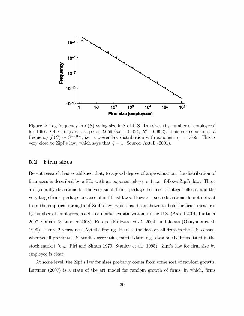
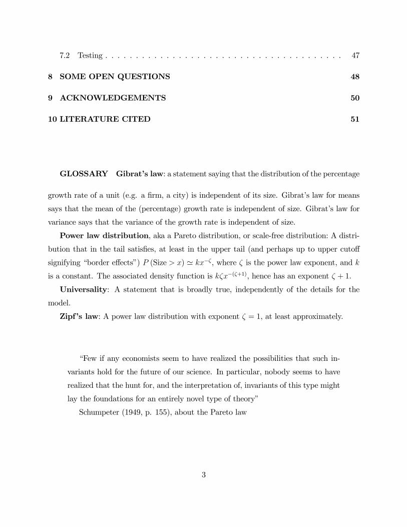
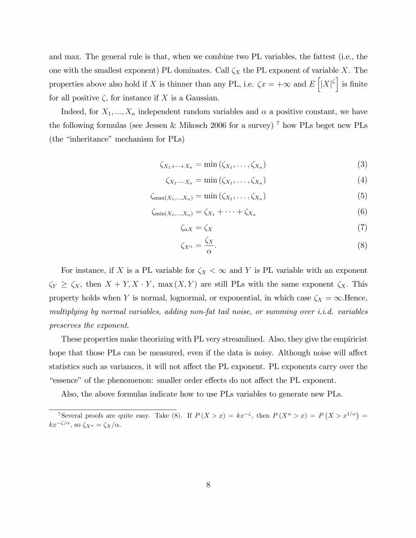
Figure 2: Log frequency ln f (S) vs log size lnS of U.S. firm sizes (by number of employees)for 1997. OLS fit gives a slope of 2.059 (s.e.= 0.054; R2 =0.992). This corresponds to afrequency f (S) ∼ S−2.059, i.e. a power law distribution with exponent ζ = 1.059. This isvery close to Zipf’s law, which says that ζ = 1. Source: Axtell (2001).
5.2 Firm sizes
Recent research has established that, to a good degree of approximation, the distribution of
firm sizes is described by a PL, with an exponent close to 1, i.e. follows Zipf’s law. There
are generally deviations for the very small firms, perhaps because of integer effects, and the
very large firms, perhaps because of antitrust laws. However, such deviations do not detract
from the empirical strength of Zipf’s law, which has been shown to hold for firms measures
by number of employees, assets, or market capitalization, in the U.S. (Axtell 2001, Luttmer
2007, Gabaix & Landier 2008), Europe (Fujiwara et al. 2004) and Japan (Okuyama et al.
1999). Figure 2 reproduces Axtell’s finding. He uses the data on all firms in the U.S. census,
whereas all previous U.S. studies were using partial data, e.g. data on the firms listed in the
stock market (e.g., Ijiri and Simon 1979, Stanley et al. 1995). Zipf’s law for firm size by
employee is clear.
At some level, the Zipf’s law for sizes probably comes from some sort of random growth.
Luttmer (2007) is a state of the art model for random growth of firms: in which, firms
30
receive an idiosyncratic productivity shocks at each period. Firms exit if they become too
unproductive, endogenizing the lower barrier. Luttmer shows a way in which, when imitation
costs become very small, the PL exponent goes to 1. Other interesting models include Rossi-
Hansberg &Wright (2007b), which is geared towards plants with decreasing returns to scale,
and Acemoglu and Cao (2009), which focuses on innovation process.
Zipf’s law for firms immediately suggests some consequences. The size of bankrupt firms
might be approximately Zipf: this is what Fujiwara (2004) finds in Japan. The size of
strikes should also follow approximately Zipf’s law, as Biggs (2005) finds for the late 19th
century. The distribution of the “input output network” linking sectors (which might be
Zipf distributed, like firms) might be Zipf distributed, as Carvalho (2008) finds.
Does Gibrat’s law for firm growth hold? There is only a partial answer, as most of the
data comes from potentially non-representative samples, such as Compustat (firms listed in
the stock market). Within Compustat, Amaral et al. (1997) find that the mean growth rate,
and the probability of disappearance, are uncorrelated with size. However, they confirm
the original finding of Stanley et al. (1996) that the volatility does decay a bit with size,
approximately at the power −1/6.18It remains unclear if this finding will generalize to thefull sample: it is quite plausible that the smallest firms in Compustat are amongst the most
volatile in the economy (it is because they have large growth options that firms are listed in
the stock market), and this selection bias would create the appearance of a deviation from
Gibrat’s law for standard deviations. There is an active literature on the topic, see Fu et al.
(2005) and Sutton (2007).
5.3 City sizes
The literature on the topic of city size is vast, so only some key findings are mentioned.
Gabaix & Ioannides (2004) provide a fuller survey. City sizes hold a special status, because
of the quantity of very old data. Zipf’s law generally holds to a good degree of approximation
(with an exponent within 0.1 or 0.2 of 1, see Gabaix & Ioannides 2004; Soo 2005). Generally,
18This may help explain Mulligan (1997). If the proportional volatility of a firm of size S is σ ∝ S−1/6,and the cash demand by that firm is proportional to σS, then the cash demand is S5/6, close to Mulligan’sempirical finding.
31
the data comes from the largest cities in a country, typically because those are the ones with
good data.
Two recent developments have changed this perspective. First, Eeckhout (2004), using
all the data on U.S. administrative cities, finds that the distribution of administrative city
size is captured well by a lognormal distribution, even though there may be deviations in the
tails. Second, in ongoing work, Makse et al. (2008), using a new procedure to classify cities
based on micro data (a “burning” algorithm that builds clusters as cities), find, however,
that city sizes follow Zipf’s law to a surprisingly good accuracy, in the US and the UK.
For cities, Gibrat’s law for means and variances is confirmed by Ioannides & Overman
(2003), and Eeckhout (2004). It is not entirely controversial.
This literature, while mature, appears ripe for technological process. Empirically, more
attention could be paid to measurement error, which typically will lead to finding mean-
reversion in city size and lower population volatility for large cities. Also, for the logic
of Gibrat’s law to hold, it is enough that there is a unit root in the log size process in
addition to transitory shocks that may obscure the empirical analysis (Gabaix & Ioannides
2004). Hence, one can imagine that the next generation of city evolution empirics could
draw from the sophisticated econometric literature on unit roots developed in the past two
decades. Theorectically, new empirical results will no doubt demand amendment of the
models. Second, the models do not connect seamlessly with the issues of “geography”
(Brakman et al. 2009), including the link to trade, issues of center and periphery and the
like. Now that the core “Zipf” issue is more or less in place, adding even more economics to
the models seems warranted.
Zipf’s law has generated many models with economic microfoundations. Krugman (1996)
proposes that natural advantages might follow a Zipf’s law. Gabaix (1999) uses “amenity”
shocks to generate the proportional random growth of population with a minimalist economic
model. Gabaix (1999a) examines how extensions of such a model can be compatible with
unbounded positive or negative externalities. Cordoba (2008) clarifies the range of economic
models that can accommodate Zipf’s law. The next two papers consider the dynamics of
industries that host cities. Rossi-Hansberg & Wright (2007a) generate a PL distribution
of cities with a random growth of industries, and birth-death of cities to accommodate
32
that growth (see also Benguigui & Blumenfeld-Lieberthal 2007 for a model with birth of
cities). Duranton (2007)’s model has several industries per city and a quality ladder model
of industry growth. He obtains a steady state distribution that is not Pareto, but can
approximate a Zipf’s law under some parameters. Finally, Hsu (2008) uses a “central place
hierarchy” model that does not rely on random growth, but instead on a static model using
the PL spacings of section 4.2.
Mori et al. (2008) document a new fact: if Si is the average size of cities hosting industry
i, and Ni the number of such cities, they find that Si ∝ N−βi , for a β ' 3/4. This sort of
relation is bound to help constraining new theories of urban growth.
5.4 Income and wealth
The first documented empirical facts about the distribution of wealth and income are the
Pareto laws of income and wealth, which state that the tail distributions of income and
wealth are PL. The tail exponent of income seems to vary between 1.5 and 3. It is now very
well documented, thanks to the data efforts reported in Atkinson & Piketty (2007).
There is less cross-country evidence on the exponent of the wealth distribution, because
the data is harder to find. It seems that the tail exponent of wealth is rather stable, perhaps
around 1.5. See Klass et al. (2006) for the Forbes 400 in the US and Nirei & Souma (2007,
Fig. 6) for Japan. In any case, almost all studies find that the wealth distribution is more
unequal than the income distribution.
Starting with Champernowne (1953), Simon (1955), Wold & Whitlle (1957), and Man-
delbrot (1961), many models have been proposed to explain the tail distribution of wealth,
mainly along the lines of random growth. See Levy (2003) and Benhabib & Bisin (2007) for
recent models. Still, it is still not clear why the exponent for wealth is rather stable across
economies. An exponent of 1.5-2.5 doesn’t emerge “naturally” out of an economic model:
rather, models can accommodate that, but they can also accommodate exponents of 1.2, or
5, or 10.
One may hope that the recent accumulation of empirical knowledge reported in Atkinson
& Piketty (2007) will contribute to a spur in the understanding of wealth dynamics. One
conclusion from the Atkinson & Piketty studies is that many important features (e.g. move-
33
ments in tax rates, wars that wipe out part of wealth) are actually not in most models, so
that models are ripe for an update.
For the bulk of the distribution, below the upper tail, a variety of shapes have been
proposed. Dragulescu & Yakovenko (2001) propose an exponential fit for personal income:
in the bulk of the income distribution, income follows a density ke−kx. This is accomplished
through a random growth model.
5.5 Roberts’ law for CEO compensation
Starting with Roberts (1956), many empirical studies (e.g., Baker et al. 1988; Barro & Barro
1990; Cosh 1975; Frydman & Saks 2007; Kostiuk 1990; and Rosen 1992) document that CEO
compensation increases as a power function of firm size w ∼ Sκ, in the cross-section. Baker
et al. (1988, p.609) call it “the best documented empirical regularity regarding levels of
executive compensation.” Typically the exponent κ is around 1/3 — generally, between 0.2
and 0.4. Hierarchical and matching models generate this scaling as in eq. 34, but there is
no compelling explanation for why the exponent should be around 1/3. The Lucas (1978)
model of firms predicts κ = 1 (see Gabaix & Landier 2008).
6 EMPIRICAL POWER LAWS: RECENTLY PRO-
POSED LAWS
6.1 Finance: PLs of stock market activity
New large-scale financial datasets have led to progress in the understanding of the tail of
financial distributions, pioneered by Mandelbrot (1963) and Fama (1963).19 Key work was
done by physicist H. Eugene Stanley’s group at Boston University, which spawned a large
literature in econophysics. This literature goes beyond previous research by using very large
datasets.
19They conjectured a Lévy distribution of stock market returns, but as we will see, the tails appeared tobe less fat than a Lévy.
34
The “Cubic Law” Distribution of Stock Price Fluctuations: ζr ' 3 The tail
distribution of short term (a few minutes to a few days) returns has been analyzed in a
series of studies that use an ever increasing number of data points (Jansen & de Vries 1991,
Mantegna & Stanley 1995, Lux 1996). Gopikrishnan et al. (1999) using a very large number
of data points established a very large presumption for a “cubic” power law of stock market
returns.20 Let rt denote the logarithmic return over a time interval ∆t.21 Gopikrishnan et
al. (1999) find that the distribution function of returns for the 1,000 largest U.S. stocks and
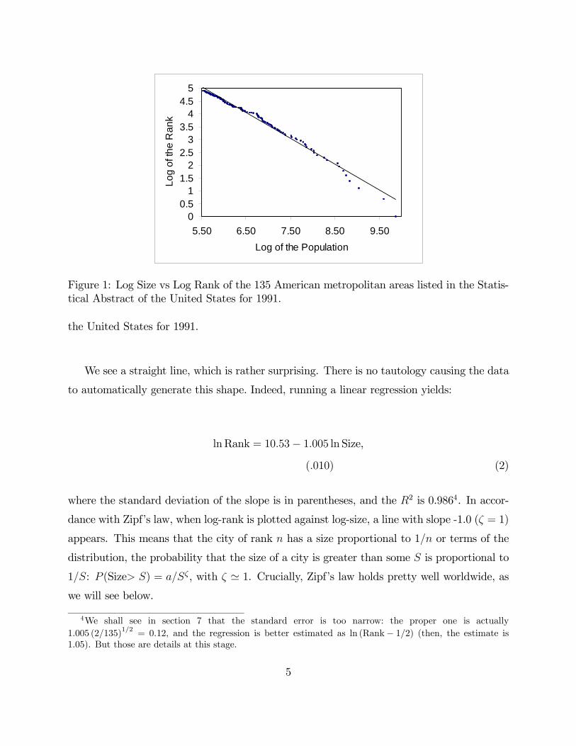
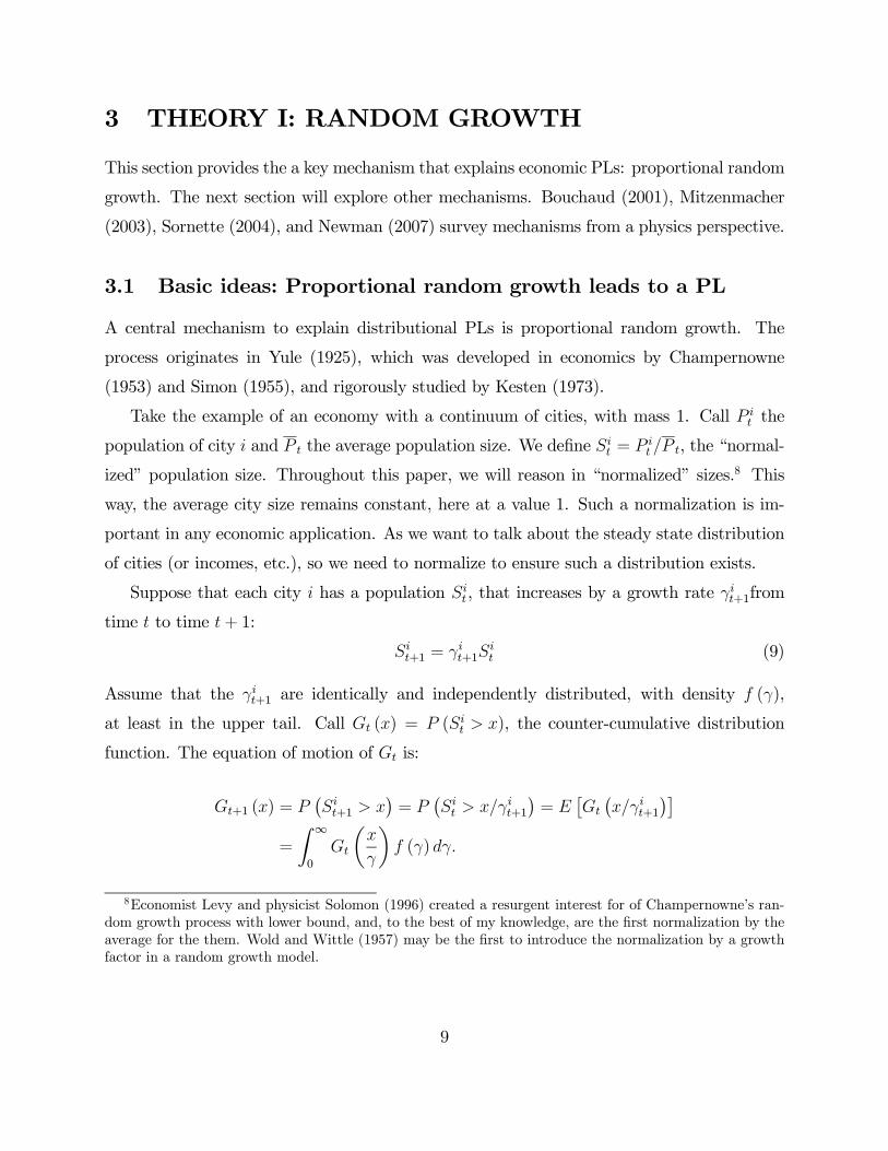
several major international indices is:
P (|r| > x) ∝ 1
xζrwith ζr ' 3. (38)
This relationship holds for positive and negative returns separately and is illustrated in
Figure 3. It plots the cumulative probability distribution of the population of normalized
absolute returns, with lnx on the horizontal axis and lnP (|r| > x) on the vertical axis. It
shows that
lnP (|r| > x) = −ζr lnx+ constant (39)
yields a good fit for |r| between 2 and 80 standard deviations. OLS estimation yields −ζr =−3.1±0.1, i.e., (38). It is not automatic that this graph should be a straight line, or that theslope should be −3: in a Gaussian world it would be a concave parabola. Gopikrishnan et al.(1999) call Equation 38 “the cubic law” of returns. The particular value ζr ' 3 is consistentwith a finite variance, and means that stock market returns are not Lévy distributed (a Lévy
distribution is either Gaussian, or has infinite variance, ζr < 2). 22
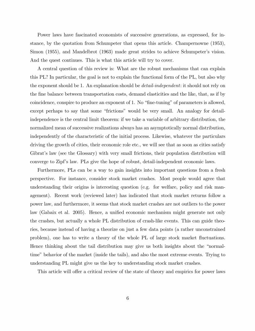
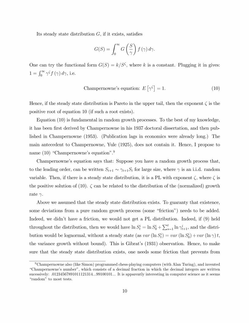
Plerou et al. (1999) examine firms of different sizes. Small firms have higher volatility
than large firms, as is verified in Figure 4a. Moreover, the same diagram also shows similar
20Here I can only cite a small number of the interesting papers of by Stanley’s group. Seehttp://polymer.bu.edu/hes/ for more papers by the same team.21To compare quantities across different stocks, variables such as r and q are normalized by the second
moments if they exist, otherwise by the first moments. For instance, for a stock i, the normalized return isr0it = (rit − ri) /σr,i, where ri is the mean of the rit and σr,i is their standard deviation. For volume, whichhas an infinite standard deviation, the normalization is q0it = qit/qi, where qit is the raw volume, and qi isthe absolute deviation: qi = |qit − qit|.22In the reasoning of Lux & Sornette (2002), it also means that stock market crashes cannot be the
outcome of simple rational bubbles.
35
slopes for the graphs of all four distributions. Figure 4b normalizes the distribution of
each size quantile by its standard deviation, so that the normalized distributions all have a
standard deviation of 1. The plots collapse on the same curve, and all have exponents close
to ζr ' 3.
Insert Figure 4 here
Such a fat-tail PL yields a large number of tail events. Considering that the typical
standard daily deviation of a stock is about 2%, a 10 standard deviation event is a day in
which the stock price moves by at least 20%. The reader can see from day to day experience
that those moves are not rare at all: essentially every week contains a 10 standard deviation
happens for one of the stocks in the market. The cubic law quantifies that notion. It also
says that a 10 standard deviations event and 20 standard deviations event are, respectively,
53 = 125 and 103 = 1000 times less likely than a 2 standard deviation event.
Equation 38 also appears to hold internationally (Gopikrishnan et al. 1999). Further-
more, the 1929 and 1987 “crashes” do not appear to be outliers to the PL distribution of
daily returns (Gabaix et al. 2005). Thus there may not be a need for a special theory of
“crashes”: extreme realizations are fully consistent with a fat-tailed distribution. This gives
the hope that a unified mechanism might account for market movements, big and small, and
including crashes.
The above results hold for relatively short time horizons — a day or less. Longer-horizon
return distributions are shaped by two opposite forces. One force is that a finite sum of
independent PL distributed variables with exponent ζ is also PL distributed, with the same
exponent ζ. If the time-series dependence between returns is not too large, one expects the
tails of monthly and even quarterly returns to remain PL distributed. The second force
is the central limit theorem, which says that if T returns are aggregated, the bulk of the
distribution converges to Gaussian. In sum, as we aggregate over T returns, the central
part of the distribution becomes more Gaussian, while the tail return distribution remains
a PL with exponent ζ but have an ever smaller probability, so that they may not even be
detectable in practice.
36
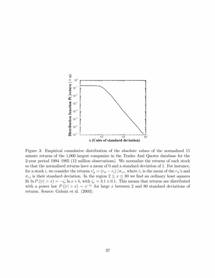
Figure 3: Empirical cumulative distribution of the absolute values of the normalized 15minute returns of the 1,000 largest companies in the Trades And Quotes database for the2-year period 1994—1995 (12 million observations). We normalize the returns of each stockso that the normalized returns have a mean of 0 and a standard deviation of 1. For instance,for a stock i, we consider the returns r0it = (rit − ri) /σr,i, where ri is the mean of the rit’s andσr,i is their standard deviation. In the region 2 ≤ x ≤ 80 we find an ordinary least squaresfit lnP (|r| > x) = −ζr lnx+ b, with ζr = 3.1± 0.1. This means that returns are distributedwith a power law P (|r| > x) ∼ x−ζr for large x between 2 and 80 standard deviations ofreturns. Source: Gabaix et al. (2003).
37
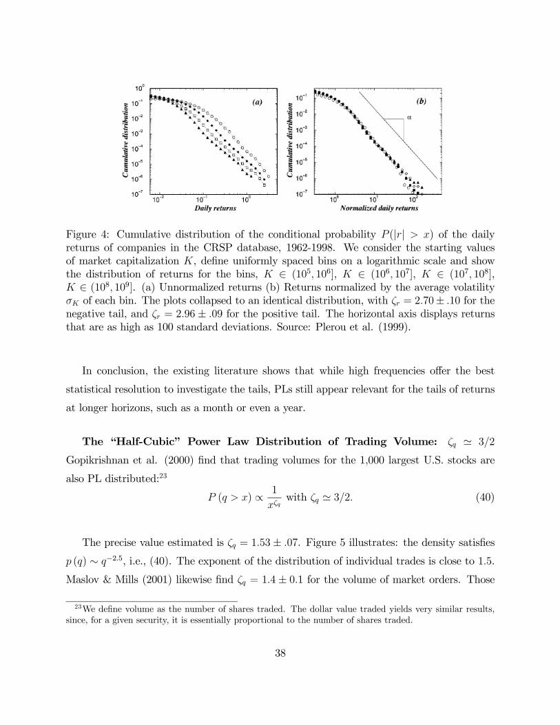
Figure 4: Cumulative distribution of the conditional probability P (|r| > x) of the dailyreturns of companies in the CRSP database, 1962-1998. We consider the starting valuesof market capitalization K, define uniformly spaced bins on a logarithmic scale and showthe distribution of returns for the bins, K ∈ (105, 106], K ∈ (106, 107], K ∈ (107, 108],K ∈ (108, 109]. (a) Unnormalized returns (b) Returns normalized by the average volatilityσK of each bin. The plots collapsed to an identical distribution, with ζr = 2.70± .10 for thenegative tail, and ζr = 2.96 ± .09 for the positive tail. The horizontal axis displays returnsthat are as high as 100 standard deviations. Source: Plerou et al. (1999).
In conclusion, the existing literature shows that while high frequencies offer the best
statistical resolution to investigate the tails, PLs still appear relevant for the tails of returns
at longer horizons, such as a month or even a year.
The “Half-Cubic” Power Law Distribution of Trading Volume: ζq ' 3/2
Gopikrishnan et al. (2000) find that trading volumes for the 1,000 largest U.S. stocks are
also PL distributed:23
P (q > x) ∝ 1
xζqwith ζq ' 3/2. (40)
The precise value estimated is ζq = 1.53± .07. Figure 5 illustrates: the density satisfies
p (q) ∼ q−2.5, i.e., (40). The exponent of the distribution of individual trades is close to 1.5.
Maslov & Mills (2001) likewise find ζq = 1.4 ± 0.1 for the volume of market orders. Those
23We define volume as the number of shares traded. The dollar value traded yields very similar results,since, for a given security, it is essentially proportional to the number of shares traded.
38
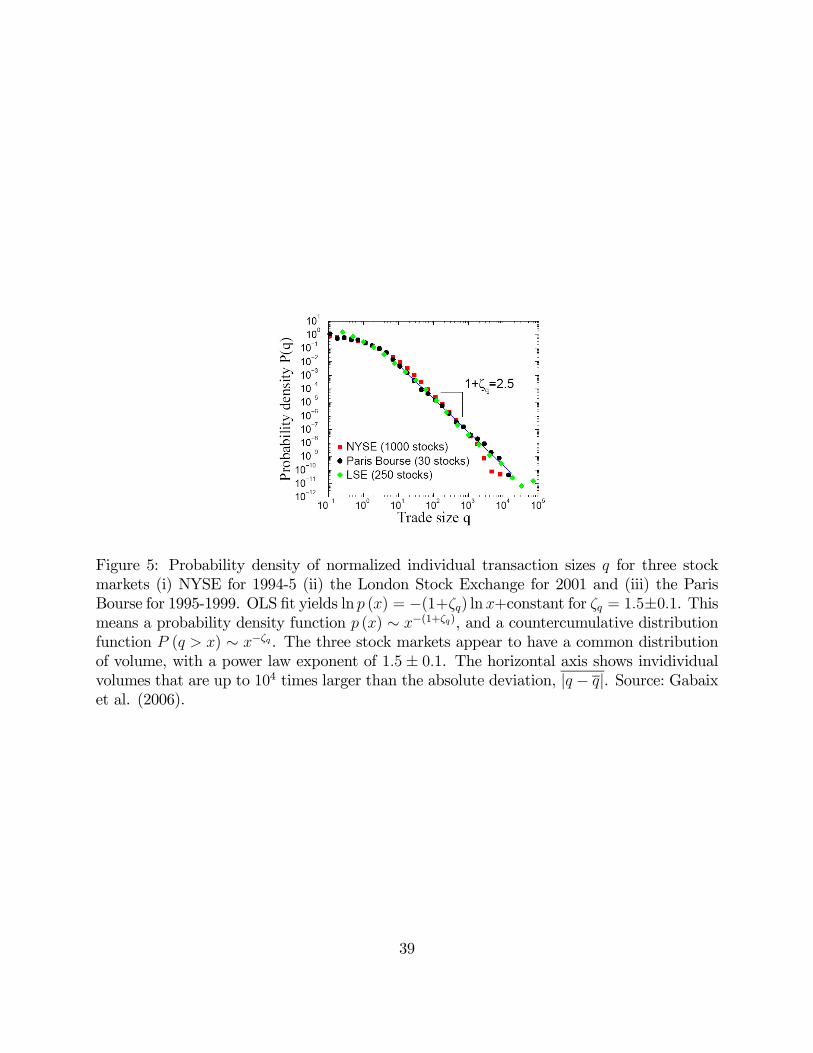
Figure 5: Probability density of normalized individual transaction sizes q for three stockmarkets (i) NYSE for 1994-5 (ii) the London Stock Exchange for 2001 and (iii) the ParisBourse for 1995-1999. OLS fit yields ln p (x) = −(1+ζq) lnx+constant for ζq = 1.5±0.1. Thismeans a probability density function p (x) ∼ x−(1+ζq), and a countercumulative distributionfunction P (q > x) ∼ x−ζq . The three stock markets appear to have a common distributionof volume, with a power law exponent of 1.5 ± 0.1. The horizontal axis shows invidividualvolumes that are up to 104 times larger than the absolute deviation, |q − q|. Source: Gabaixet al. (2006).
39
U.S. results are extended to France and the UK in Gabaix et al. (2006): 30 large stocks of
the Paris Bourse from 1995—1999, which contain approximately 35 million records, and 250
stocks of the London Stock Exchange in 2001. As shown in Figure 5, we find ζq = 1.5± 0.1for each of the three stock markets. The exponent appears essentially identical in the three
stock markets, which is suggestive of universality.
Other Power Laws Finally, the number of trades executed over a short horizon has
an exponent around 3.3 (Plerou et al. 2000).
Some Proposed Explanations There is no consensus about the origins for those
regularities. Indeed, there are few models making testable predictions about the fat-tailness
of stock market returns.
ARCH. The fat tail of returns could come from ARCH effects, as we mentioned in section
3.3. It would be very nice to have an economic model that generates such dynamics, perhaps
via a feedback rule, or the dynamics of liquidity. Ideally, it would explain the cubic and
half-cubic laws of stock market activity. However, this model does not appear to have been
written.
Trades of Large Traders. Another model was proposed in Gabaix et al. (2003, 2006).
It attributes the PLs of trading activity to the strategic trades by very large institutional
investors in relatively illiquid markets. This activity creates spikes in returns and volume,
even in the absence of important news about fundamentals, and generates the cubic and half-
cubic laws. Antecendents of this idea include Levy & Solomon (1996) express that the large
traders will have large price impact, and predict ζr = ζS (see Levy 2005 for some evidence
in that direction). Solomon and Richmond (2001) propose an amended theory, predicting
ζr = 2ζS. In the Gabaix et al. model, cost-benefit considerations lead to ζr = 3ζS, as we will
see.
Examples of that sort might be the crash of Long Term Capital Management in the
Summer 1998, the rapid unwinding of very large stock positions by Société Générale after
the Kerviel “rogue trader” scandal (which led stock markets to fall, and the Fed to cut
interest rates by 75 basis points on January 22 2008), the conjecture by Khandani & Lo
(2007) that one large fund was responsible for the crash of quantitative funds in August
40
2007, or even the crash of 1987 (see the discussion in Gabaix et al. 2006). Of course, one has
a feeling that such a theory may at most be a theory of the “impulse”, which the dynamics
of the propagation is left for future research. According to the PL hypothesis, these sort of
actions happen at all scales, including the small ones, such as day to day.
The theory works the following way. First, imagine that a trade of size q generates
a percentage price impact equal to kqγ, for a constant γ (we shall take γ = 1/2, and
sketch an explanation in the papers). A mutual fund will not want to lose more than a
certain percentage of returns in price impact (the theory microfounds that by a concern for
robustness). Each trade costs its dollar value q times the price impact, hence kq1+γ dollars.
Optimally, the fund trades as much as possible, subject to the robustness constraint. That
implies: kq1+γ ∝ S, hence the typical trade of a fund of size S is in volumes q ∝ S1/(1+γ), and
its typical price impact is |∆p| = kqγ ∝ Sγ/(1+γ). (Those predictions still await empirical
testing with micro data). Using rule (4), this generates the following PLs exponents for
returns and volumes:
ζr =
µ1 +
1
γ
¶ζS, ζγ = (1 + γ) ζS (41)
Hence the theory links the PL exponents of returns and trades to the PL exponent
of mutual funds, and price impact. Given the finding of a Zipf distribution of fund sizes
(ζS = 1, which presumably comes from random growth of funds), and a square-root price
impact (γ = 1/2), we get: ζr = 3 and ζq = 1/2, the empirically-found exponents of returns
and volumes. The theory also makes testable predictions about specific deviations from
those values.
6.2 Other scaling in finance
Bid-Ask Spread Wyart et al. (2008) offer a simple but original theory of the bid-ask
spread, which yields a new empirical prediction:
Ask− BidPrice
= kσ√N
(42)
where σ is the daily volatility of the stock, and N the average number of trades for the stock,
and k is a constant, in practice roughly close to 1. They find good support for this prediction.
41

The basic reasoning is the following (their model has more sophisticated variants): suppose
that at each trade, the log price moves by k−1 times the bid-ask spread S. After N trades,
assumed to have independent signs, the standard deviation of the log price move will be
k−1S√N . This should be the daily price move, so k−1KS
√N = σ, hence (42). Of course,
some of the microfoundations remain unclear, but at least we have a simple new hypothesis,
which makes a good scaling prediction and has empirical support. Bouchaud & Potters
(2004) and Bouchaud et al. (2009) are a very good source on scaling in finance, particularly
in microstructure.
Bubbles and the size distribution of stocks During stock market “bubbles”, it is
plausible that some stocks will be particularly overvalued. Hence, the size distribution of
stock will be more skewed. Various authors have shown this (Kou & Kou 2004, Kaizoji 2005).
It would be nice to know if, to diagnose“bubbly” markets or sectors, does this skewness of
the distribution offer a useful complement to more traditional measures such as the ratio of
market value to book value.
6.3 International Trade
In an important new result, Hinloopen & van Marrewijk (2008) find a Zipf’s law for re-
vealed comparative advantage: the “Balassa index” of revealed comparative advantage sat-
isfies Zipf’s law. Also, the size distribution of exporters might be roughly Zipf (see Helpman
et al. 2004, Figure 3)24. However, the models hitherto proposed explain a PL of the size of
exporters (Melitz 2003, Arkolakis 2008, and Chaney 2009), but not why the exponent should
be around 1. Presumably, this literature will import some ideas from the firm size literature,
to identify the root causes of the “Zipf” feature of exports.
See Eaton et al. (2004) for the beginning of a an uncovering of many powers law in the
fine structure of exports.
24In that graph, the standard errors are too narrow, because the authors use the OLS standard errors,which have a large downward bias. See section 7 for the correct standard errors, bζ (2/N)1/2.
42
6.4 Other Candidate Laws
Supply of regulations Mulligan & Shleifer (2004) establish another candidate law.
In the U.S., the quantity of regulations (as measured by the number of lines of text) is pro-
portional to the square root of the population. They provide an efficiency-based explanation
for this phenomena. It would be interesting to investigate their findings outside US states.
Scaling of CEO incentives with firm size Calling κ the Roberts’ law exponent we
saw in section 5.5,CEO Wage ∝Sκ, with κ ' 1/3 and S the firm size. Edmans et al. (2008)predict that the fraction incentives pay as a fraction of total pay is roughly independent of
firm size, and find empirical support for this prediction. If the firm value increases by 1%,
the CEO’s pay (or wealth) should increase by a percentage independent of firm size. From
this, they predict the scaling of “Jensen-Murphy” (1990) incentives: if the firm size increases
by $1000, the CEO wealth should increase by a amount proportional to S−(1−κ) = S−2/3.
The Jensen-Murphy incentives should then decline with firm size with at precise scaling. It
would be nice to investigate these scaling predictions outside the U.S.
Networks Networks are full of power laws, see Newman et al. (2006) and Jackson
(2009).
Wars Johnson et al. (2006) find that the number of death in armed conflicts follows a
PL, with an exponent around 2.5, and provide a model for it.
6.5 Power laws outside of economics
Language, and perhaps Ideas Ever since Zipf (1949), the popularity of words has
been found to follow Zipf’s law.25 There is no consensus on the origin of that regularity. One
explanation might be Simon’s (1955), or the more recent models based on Champernowne.
Another might be the “monkeys at the typewriter” (written by Mandelbrot in 1951, and
reprinted in Mandelbrot 1997 p.225). Let a monkey type randomly on a typewriter (each
25Interestingly, McCowan et al. (1999) show that Zipf’s law is not limited to human language: it holds fordolphins, those intelligent mammals.
43
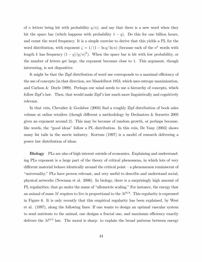
of n letters being hit with probability q/n), and say that there is a new word when they
hit the space bar (which happens with probability 1 − q). Do this for one billion hours,
and count the word frequency. It is a simple exercise to derive that this yields a PL for the
word distribution, with exponent ζ = 1/ (1− ln q/ lnn) (because each of the nk words withlength k has frequency (1− q) (q/n)k). When the space bar is hit with low probability, or
the number of letters get large, the exponent becomes close to 1. This argument, though
interesting, is not dispositive.
It might be that the Zipf distribution of word use corresponds to a maximal efficiency of
the use of concepts (in that direction, see Mandelbrot 1953, which uses entropy maximization,
and Carlson & Doyle 1999). Perhaps our mind needs to use a hierarchy of concepts, which
follow Zipf’s law. Then, that would make Zipf’s law much more linguistically and cognitively
relevant.
In that vein, Chevalier & Goolsbee (2003) find a roughly Zipf distribution of book sales
volume at online retailers (though different a methodology by Dechastres & Sornette 2005
gives an exponent around 2). This may be because of random growth, or perhaps because,
like words, the “good ideas” follow a PL distribution. In this vein, De Vany (2003) shows
many fat tails in the movie industry. Kortum (1997) is a model of research delivering a
power law distribution of ideas.
Biology PLs are also of high interest outside of economics. Explaining and understand-
ing PLs exponent is a large part of the theory of critical phenomena, in which lots of very
different material behave identically around the critical point — a phenomenon reminiscent of
“universality.” PLs have proven relevant, and very useful to describe and understand social,
physical networks (Newman et al. 2006). In biology, there is a surprisingly high amount of
PL regularities, that go under the name of “allometric scaling.” For instance, the energy that
an animal of massM requires to live is proportional to theM3/4. This regularity is expressed
in Figure 6. It is only recently that this empirical regularity has been explained, by West
et al. (1997), along the following lines: If one wants to design an optimal vascular system
to send nutrients to the animal, one designs a fractal one, and maximum efficiency exactly
delivers the M3/4 law. The moral is sharp: to explain the broad patterns between energy
44
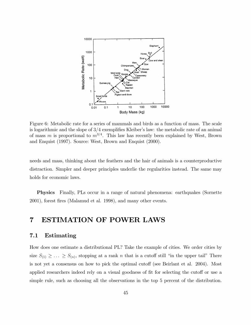
Figure 6: Metabolic rate for a series of mammals and birds as a function of mass. The scaleis logarithmic and the slope of 3/4 exemplifies Kleiber’s law: the metabolic rate of an animalof mass m is proportional to m3/4. This law has recently been explained by West, Brownand Enquist (1997). Source: West, Brown and Enquist (2000).
needs and mass, thinking about the feathers and the hair of animals is a counterproductive
distraction. Simpler and deeper principles underlie the regularities instead. The same may
holds for economic laws.
Physics Finally, PLs occur in a range of natural phenomena: earthquakes (Sornette
2001), forest fires (Malamud et al. 1998), and many other events.
7 ESTIMATION OF POWER LAWS
7.1 Estimating
How does one estimate a distributional PL? Take the example of cities. We order cities by
size S(1) ≥ . . . ≥ S(n), stopping at a rank n that is a cutoff still “in the upper tail” There
is not yet a consensus on how to pick the optimal cutoff (see Beirlant et al. 2004). Most
applied researchers indeed rely on a visual goodness of fit for selecting the cutoff or use a
simple rule, such as choosing all the observations in the top 5 percent of the distribution.
45
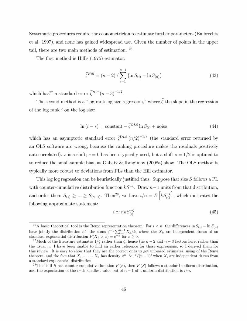
Systematic procedures require the econometrician to estimate further parameters (Embrechts
et al. 1997), and none has gained widespread use. Given the number of points in the upper
tail, there are two main methods of estimation. 26
The first method is Hill’s (1975) estimator:
bζHill = (n− 2) /n−1Xi=1
¡lnS(i) − lnS(n)
¢(43)
which has27 a standard error bζHill (n− 3)−1/2.The second method is a “log rank log size regression,” where bζ the slope in the regression
of the log rank i on the log size:
ln (i− s) = constant− bζOLS lnS(i) + noise (44)
which has an asymptotic standard error bζOLS (n/2)−1/2 (the standard error returned byan OLS software are wrong, because the ranking procedure makes the residuals positively
autocorrelated). s is a shift; s = 0 has been typically used, but a shift s = 1/2 is optimal to
to reduce the small-sample bias, as Gabaix & Ibragimov (2008a) show. The OLS method is
typically more robust to deviations from PLs than the Hill estimator.
This log log regression can be heuristically justified thus. Suppose that size S follows a PL
with counter-cumulative distribution function kS−ζ . Draw n−1 units from that distribution,and order them S(1) ≥ ... ≥ S(n−1). Then28, we have i/n = E
hkS−ζ(i)
i, which motivates the
following approximate statement:
i ' nkS−ζ(i) (45)
26A basic theoretical tool is the Rényi representation theorem: For i < n, the differences lnS(i) − lnS(n)have jointly the distribution of the sums ζ−1
Pn−1k=i Xk/k, where the Xk are independent draws of an
standard exponential distribution P (Xk > x) = e−x for x ≥ 0.27Much of the literature estimates 1/ζ rather than ζ, hence the n− 2 and n− 3 factors here, rather than
the usual n. I have been unable to find an earlier reference for those expressions, so I derived them forthis review. It is easy to show that they are the correct ones to get unbiased estimates, using of the Rényitheorem, and the fact that X1+ ...+Xn has density xn−1e−x/(n− 1)! when Xi are independent draws froma standard exponential distribution.28This is if S has counter-cumulative function F (x), then F (S) follows a standard uniform distribution,
and the expectation of the i−th smallest value out of n− 1 of a uniform distribution is i/n.
46
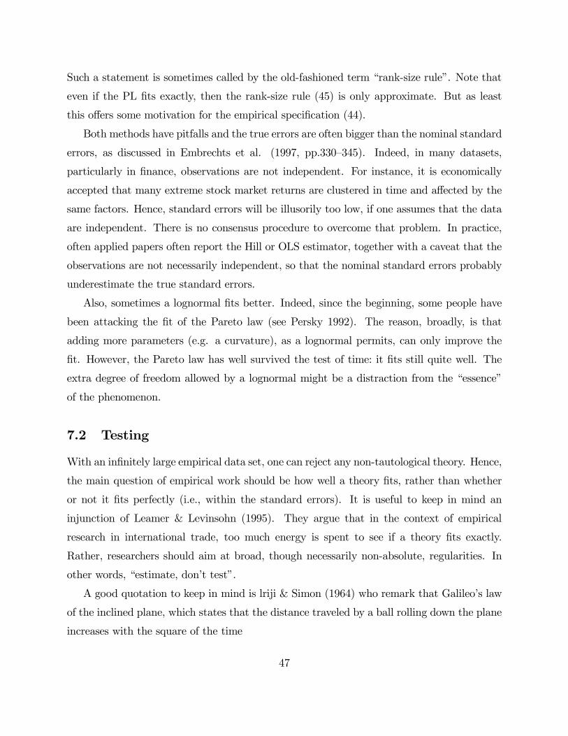
Such a statement is sometimes called by the old-fashioned term “rank-size rule”. Note that
even if the PL fits exactly, then the rank-size rule (45) is only approximate. But as least
this offers some motivation for the empirical specification (44).
Both methods have pitfalls and the true errors are often bigger than the nominal standard
errors, as discussed in Embrechts et al. (1997, pp.330—345). Indeed, in many datasets,
particularly in finance, observations are not independent. For instance, it is economically
accepted that many extreme stock market returns are clustered in time and affected by the
same factors. Hence, standard errors will be illusorily too low, if one assumes that the data
are independent. There is no consensus procedure to overcome that problem. In practice,
often applied papers often report the Hill or OLS estimator, together with a caveat that the
observations are not necessarily independent, so that the nominal standard errors probably
underestimate the true standard errors.
Also, sometimes a lognormal fits better. Indeed, since the beginning, some people have
been attacking the fit of the Pareto law (see Persky 1992). The reason, broadly, is that
adding more parameters (e.g. a curvature), as a lognormal permits, can only improve the
fit. However, the Pareto law has well survived the test of time: it fits still quite well. The
extra degree of freedom allowed by a lognormal might be a distraction from the “essence”
of the phenomenon.
7.2 Testing
With an infinitely large empirical data set, one can reject any non-tautological theory. Hence,
the main question of empirical work should be how well a theory fits, rather than whether
or not it fits perfectly (i.e., within the standard errors). It is useful to keep in mind an
injunction of Leamer & Levinsohn (1995). They argue that in the context of empirical
research in international trade, too much energy is spent to see if a theory fits exactly.
Rather, researchers should aim at broad, though necessarily non-absolute, regularities. In
other words, “estimate, don’t test”.
A good quotation to keep in mind is lriji & Simon (1964) who remark that Galileo’s law
of the inclined plane, which states that the distance traveled by a ball rolling down the plane
increases with the square of the time
47
“does ignore variables that may be important under various circumstances: irreg-
ularities in the ball or the plane, rolling friction, air resistance, possible electrical
or magnetic fields if the ball is metal, variations in the gravitational field and so
on, ad infinitum. The enormous progress that physics has made in three centuries
may be partly attributed to its willingness to ignore for a time discrepancies from
theories that are in some sense substantially correct (Ijiri & Simon 1964, p.78).”
Consistently with these suggestions, some of the debate on Zipf’s law should be cast in
terms of how well, or poorly, it fits, rather than whether it can be rejected or not. For
example, if the empirical research establishes that the data are typically well described by a
PL with exponent ζ ∈ [0.8, 1.2], then this is a useful result: It prompts to seek theoreticalexplanations of why this should be true.
Still, it is useful to have a test, so what is a test for the fit of a PL? Many papers
in practice do not provide such a test. Some authors (Clauset et al. 2008) advocate the
Kolmogorov Smirnov test. Gabaix & Ibragimov (2008b) provide a simple test based using
the OLS regression framework of the previous subsection. Define s∗ ≡cov((lnSj)2,lnSj)
2var(lnSj), and
run the OLS regression:
ln
µi− 1
2
¶= constant− bζ lnS(i) + bq ¡lnS(i) − s∗
¢2+ noise (46)
to estimate the values bζ and bq. The term (lnSi − s∗)2 captures a quadratic deviation from
an exact PL. The coefficient s∗ recenters the quadratic term: with it the estimate of the PL
exponents bζ is the same whether the quadratic term is included or not. The test of the PL
is: Reject the null of an exact PL iff¯̄̄bq/bζ2 ¯̄̄ > 1.95 · (2n)−1/2.
8 SOME OPEN QUESTIONS
I conclude with some open questions. By the Schumpeter quote that opens this review,
answering such a question might lead to a different point of view on the issue in question,
e.g. the nature of capital and technological progress for question or the origin of stock market
crashes.
48
Theory
1. Is there a “deep” explanation for the coefficient of 1/3 capital share in the aggregate
capital stock? This constancy is one of the most remarkable regularities in economics.
It is a pity that it does not have an explanation. A fully satisfactory explanation should
not only generate the constant capital share, but some reason why the exponent should
be 1/3 ? See Jones (2005) for an interesting paper that generates a Cobb-Douglas, but
does not predict the 1/3 exponent. With such an answer, we might understand more
deeply what causes technological progress or the nature of capital
2. Can we explain fully the PL distribution of financial variables, particularly returns
and trading volume? This article sketched some theories, but they are at best partial.
Working out a fully theory of large financial movements, guided by PLs, might be a
surprising key to the explanation of both “excess volatility” and financial crashes, and,
perhaps appropriate risk-management or policy responses.
3. Is there an explanation for the PL distribution of firms that is not based on a simple
“mechanical” Gibrat’s law, but instead comes from full efficiency maximization? For
instance, in biology, we have seen relations (West et al. 1997) that show that PLs come
as a way to maximize efficiency: that is, roughly, because an organization in network,
with a scale-free (fractal) organization, is optimal under many circumstances. It is
plausible that the same happens in economics: solving this conjecture would be very
interesting. Of course, the same may hold for the Zipf’s law for words: it might be
that the Zipf distribution of word use corresponds to a maximal efficiency of the use
of concepts.
4. Is there a “deep” explanation for the coefficient of 1/3 in the Roberts’ law listed in
section 5.5? Some theories predict a relation w ∝ Sκ, for some κ between 0 and 1, but
none predicts why the exponent should be (roughly) 1/3. Gabaix & Landier (2008)
show that the exponent 1/3 arises if the distribution of talents has a square root
shaped upper bound. Is there any “natural” mechanism, perhaps random growth for
the accumulation or detection of talent, that would generate that distribution? With
49

such an insight, we might understand better how top talent (which may be a crucial
engine in growth) is accumulated.
5. Is there a way to generate macroeconomic fluctuations, purely from microeconomic
shocks? Bak et al. (1993) contains a rather fascinating possibility, in which inventory
needs propagate throughout the economy. Nirei (2006) is a related model. Those mod-
els have not yet convinced all economists, as they do not yet make tight predictions
and they tend to generate too fat tailed fluctuations (they are Lévy distributions with
infinite variance). Still, they might be on the right track. Gabaix (2007)’s theory
of “granular fluctuations” generates fluctuations from the existence of large firms or
sectors (see also Brock and Durlauf 1991, Durlauf 1993). These models are still hy-
potheses. Better understanding the origins of macroeconomic fluctuations should lead
to better models and policies.
Empirics
6. Do tail events matter for investors, in particular for risk premia? Various authors
have argued that they do (Barro 2006, Gabaix 2008, Ibragimov et al. forthcoming,
Weitzman 2007), but this is a matter of ongoing research.
7. Economics of superstars: It would be good to test “superstars” models, and see if the
link between stakes (e.g. advertising revenues), talents (e.g. ability of a golfer) and
income is as predicted by theories.
8. The availability of large new datasets makes it possible to discover new PLs, and test
the models’ predictions about microeconomic behavior. Times seem ripe for economists
to use those PLs, and renew the tradition of Gibrat, Champernowne, Mandelbrot and
Simon, and investigate old and new regularities with renewed models and data.
9 ACKNOWLEDGEMENTS
This work was supported NSF grant 0527518. I thank Esben Hedegaard and Rob Tumarking
for very good research assistance, Jonathan Parker for the Schumpeter quote, Alex Edmans,
50
Moshe Levy, Sorin Solomon, Gene Stanley for helpful comments.
10 LITERATURE CITED
Acemoglu, D, Cao D. 2008. Innovation by Entrants and Incumbents. Work. Pap. Massa-
chusetts Institute of Tech.
Amaral LAN, Buldyrev SV, Havlin S, Leschhorn H, Maass P, Salinger MA, Stanley HE,
Stanley MHR. 1997. Scaling behavior in economics: I. Empirical results for company growth.
J. de phys. (France) I. 7:621-33
Arkolakis C. 2008. Market penetration costs and trade dynamics. Work. Pap., Dep.
Econ., Yale Univ.
Atkinson AB, Piketty T. 2007. Top incomes over the twentieth century. Oxford: Oxford
University Press
Auerbach F. 1913. Das Gesetz der Bevölkerungskonzentration. Petermanns Geogr. Mitt.
59:74—76
Axtell R. 2001. Zipf distribution of U.S. firm sizes. Science, 293:1818-20
Bak P, Chen K, Woodford M. 1993. Aggregate fluctuations from independent sectoral
shocks: Self-organized criticality in a model of production and inventory dynamics. Ricerche
Econ. 47:3-30
Baker G, Jensen M, Murphy K. 1988. Compensation and incentives: practice vs. theory.
J. of Financ. 43:593-616
Barabási AL, Albert R. 1999. Emergence of scaling in random networks. Science.
286:509-12
Barro RJ. 2006. Rare disasters and asset markets in the twentieth century. Q. J. of
Econ.. 121: 823-866
Barro J, Barro RJ. 1990. Pay, performance, and turnover of bank CEOs. J. of Labor
Econ. 8:448-81
Beirlant J, Goegebeur Y, Segers J, Teugels J. 2004. Statistics of Extremes: Theory and
Applications, England: Wiley
Benhabib J, Bisin A. 2007. The distribution of wealth: intergenerational transmission
51
and redistributive policies. Work. Pap., New York Univ.
Benguigui L, Blumenfeld-Lieberthal E. 2007. A dynamic model for city size distribution
beyond Zipf ’s law. Physica A 384:613—27
Biggs M. 2005. Strikes as forest fires: Chicago and Paris in the late nineteenth century.
Am. J. Sociolog. 110:1684—1714
Bouchaud, JP. 2001. Power-laws in Economics and Finance: Some Ideas from Physics.
Quant. Fin. 1:105.
Bouchaud JP, Farmer JD, Lillo F. 2009. How markets slowly digest changes in supply
and demand. In Handbook of Financial Markets: Dynamics and Evolution, ed. T Hens, KR
Schenkhoppe. Academic Press
Bouchaud, JP, Potters, M. 2004. Theory of Financial Risk and Derivative Pricing: From
Statistical Physics to Risk Management. Cambridge University Press.
Brakman S, Garretsen H, van Marrewijk C. 2009. An Introduction to Geographical Eco-
nomics, Cambridge: Cambridge Univ. Press 2nd ed.
Brock, W, Durlauf S. 2001. Discrete choice with social interactions. Review of Economic
Studies, 68:235—60.
Brown JH, West GB, eds. 2000. Scaling in Biology, Oxford: Oxford Univ. Press
Carlson JM, Doyle J. 1999. Highly optimized tolerance: A mechanism for power laws in
designed systems. Phys. Rev. E 60:1412-27
Carroll G. 1982. National city-size distributions: what do we know after 67 years of
research?. Prog. in Hum. Geogr. 6:1-43
Carvalho V. 2008. Aggregate fluctuations and the network structure of intersectoral
trade. Work. Pap., Univ. of Chicago
Challet D, Marsili M, Zhang YC. 2005. Minority Games: Interacting Agents in Financial
Markets. Oxford University Press.
Champernowne D. 1953. A model of income distribution. Econ. J. 83: 318-51
Chaney T. 2009. Distorted gravity: The intensive and extensive margins of international
trade. Am. Econ. Rev. In press.
Chevalier J, Goolsbee A. 2003. Measuring prices and price competition online: Amazon
and Barnes and Noble. Quant. Mark. and Econ.. 1:203-222
52
Clauset A, Shalizi CR, Newman MEJ. 2008. Power-law distributions in empirical data.
Work. Pap., Santa Fe Institute.
Cordoba J. 2008. On the distribution of city sizes, J. of Urban Econ. 63:177-97
Cosh A. 1975. The renumeration of chief executives in the United Kingdom. Econ. J.
85:75—94
Deschatres F and Sornette D. 2005. The Dynamics of Book Sales: Endogenous versus
Exogenous Shocks in Complex Networks. Phys. Rev. E. 72:016112.
De Vany, A. 2003. Hollywood Economics. Routledge
Di Guilmi C, Aoyama H, Gallegati M, Souma W. 2004. Do Pareto—Zipf and Gibrat laws
hold true? An analysis with European firms. Phys. A. 335:197-216
Dragulescu A, Yakovenko VM. 2001. Evidence for the exponential distribution of income
in the USA. The Eur. Phys. J. B. 20:585-9
Duranton G. 2006. Some foundations for Zipf ’s law: Product proliferation and local
spillovers. Reg. Sci. and Urban Econ. 36:542—63
Duranton G. 2007. Urban evolutions: The fast, the slow, and the still. Am. Econ. Rev.
97:197-221
Durlauf, S. 1993. Nonergodic Economic Growth. Rev. Econ. Stud. 60:349-66.
Durlauf, S. 2005. Complexity and Empirical Economics. Econ. J. , 115:F225-243.
Eaton J, Kortum S, Kramarz F. 2004. Dissecting trade: Firms, industries, and export
destinations. Am. Econ. Rev. Pap. and Proc.. 94:150-4
Edmans A, Gabaix X, Landier A. 2008. A multiplicative model of optimal CEO incentives
in market equilibrium.Work. Pap., SSRN.
Embrechts P, Kluppelberg C, Mikosch T. 1997. Modelling Extremal Events for Insurance
and Finance, New York: Springer
Estoup JB. 1916. Les gammes sténographiques, Paris: Institut Sténographique
Fama, E. 1963. “Mandelbrot and the Stable Paretian Hypothesis,” Journal of Business,
36:420-429.
Frydman C, Saks R. 2007. Historical trends in executive compensation, 1936-2003. Work.
Pap., Harvard Univ.
Fu, D., F. Pammolli, S. V. Buldyrev, M. Riccaboni, K. Matia, K. Yamasaki, and H. E.
53
Stanley. 2005. The growth of business firms: theoretical framework and empirical evidence.
Proc. Natl. Acad. Sci. USA 102:18801-6.
Fujiwara Y. 2004. Zipf law in firms bankruptcy. Phys. A: Stat. and Theor. Phys..
337:219-30
Gabaix X. 1999. Zipf’s law for cities: An explanation. Q. J. of Econ. 114:739-67
Gabaix, X. 1999a. Zipf’s Law and the Growth of Cities, Am. Econ. Rev., Papers and
Proceedings, 89:129-32.
Gabaix X. 2007. The granular origins of aggregate fluctuations. Work. Pap., New York
Univ.
Gabaix X. 2008. Variable rare disasters: A tractable theory of ten puzzles in macro-
finance.Am. Econ. Rev. Papers and Proc., 98:64-67.
Gabaix X, Gopikrishnan P, Plerou V, Stanley HE. 2003. A theory of power law distrib-
utions in financial market fluctuations. Nature, 423:267—230
Gabaix X, Gopikrishnan P, Plerou V, Stanley HE. 2005. Are stock market crashes out-
liers?. Work. Pap.. Massachusetts Institute of Tech.
Gabaix X, Gopikrishnan P, Plerou V, Stanley HE. 2006. Institutional investors and stock
market volatility. Q. J. of Econ.. 121:461-504
Gabaix X, Ibragimov R. 2008a. Rank-1/2: A simple way to improve the OLS estimation
of tail exponents. Work Pap., NBER
Gabaix X, Ibragimov R. 2008b. A simple OLS test of power law behavior. Work. Pap.,
Harvard Univ.
Gabaix X, Ioannides Y. 2004. The evolution of the city size distributions. In Handbook of
Regional and Urban Economics, eds. V Henderson, JF Thisse, 4:2341-78. Oxford: Elsevier
Science
Gabaix X, Landier A. 2008. Why has CEO pay increased so much?. Q. J. of Econ.
123:49-100
Gibrat R. 1931. Les inégalités économiques, Paris: Librairie du Recueil Sirey
Gopikrishnan P, Plerou V, Amaral L, Meyer M, Stanley HE. 1999. Scaling of the distri-
bution of fluctuations of financial market indices. Phys. Rev. E. 60:5305-5316
Gopikrishnan P, Gabaix X, Plerou V, Stanley HE. 2000. Statistical properties of share
54
volume traded in financial markets. Phys. Rev. E. 62:R4493-R4496
Goldie CM. 1991. Implicit renewal theory and tails of solutions of random equations.
The Ann. of Appl. Probab.. 1:126-66
Helpman E, Melitz MJ, Yeaple SR. 2004. Export versus FDI with heterogeneous firms.
Am. Econ. Rev. 94:300-16
Hill BM. 1975. A simple approach to inference about the tail of a distribution. Ann. of
Stat. 3:1163—74
Hinloopen J, Van Marrewijk C. 2008. Comparative advantage, the rank-size rule, and
Zipf’s law. Work. Pap., Tinbergen Institute
Hsu W. 2008. Central place theory and Zipf’s law. Work. Pap., Univ. of Minnesota
Ibragimov R, JaffeeW,Walden J. 2008. Nondiversification traps in catastrophe insurance
markets. Rev. of Financ. Stud. In press
Ijiri Y, Simon HA. 1964. Business firm growth and size. The Am. Econ. Rev. 54:77-89
Ijiri Y, Simon HA. 1979. Skew Distributions and the Sizes of Business Firms, eds. North-
Holland.
Ioannides YM, Overman HG. 2003. Zipf’s law for cities: An empirical examination. Reg.
Sci. and Urban Econ. 33:127—37
Jackson, M. The Theory of Networks. Annual Review of Economics 1.
Jansen, D, de Vries, C. 1991. On the Frequency of Large Stock Returns: Putting Booms
and Busts into Perspective. Review of Economics and Statistics. 73:18-24.
Jensen M, Murphy KJ. 1990. Performance pay and top-management incentives. J. of
Polit. Econ.. 98:225-64
Jessen AH, Mikosch T. 2006. Regularly varying functions. Publ. de l’Inst. Math.
94:171—92
Johnson NF, Spagat M, Restrepo JA, Becerra O, et al. 2006. Universal patterns under-
lying ongoing wars and terrorism. Work. Pap.. Univ. Miami
Jones C. 2005. The shape of production functions and the direction of technical change.
Quart. J. Ec. 120:517-49
Kaizoji, T. 2006. A precursor of market crashes: Empirical laws of Japan’s internet.
Eur. Phys. J. B 50:123—127
55
Kesten H. 1973. Random difference equations and renewal theory for products of random
matrices. Acta Math. 131:207-248
Khandaniy AE, Lo AW. 2007. What happened to the quants in August 2007? Work.
Pap., Massachusetts Institute of Tech.
Kortum SS. 1997. Research, patenting, and technological change. Econometrica. 65:1389-
1419
Kostiuk PF. 1990. Firm size and executive compensation. J. of Human Resources. 25:91—
105
Kou, SC and Kou SG. 2004. A diffusion model for growth stocks. Math. of Oper. Res.
29:191—212
Klass O, Biham O, Levy M, Malcai O, Solomon S. 2006. The Forbes 400 and the Pareto
wealth distribution. Econ. Lett. 90:290-5
Krugman P. 1996. Confronting the mystery of urban hierarchy. J. of the Jpn. and Int.
Econ.. 10:399-418
Leamer E, Levinsohn J. 1995. International trade theory: The evidence. In Handbook
of International Economics, eds. G Grossman, K. Rogoff, 3:1339-94. Amsterdam: North-
Holland
Levy M. 2003. Are rich people smarter?. J. of Econ. Theor. 110:42—64
Levy M. 2005. Market efficiency, the Pareto wealth distribution, and the Lévy distribu-
tion of stock returns. In The Economy as an Evolving Complex System, eds. S Durlauf, L
Blume, Oxford: Oxford University Press
Levy M, Solomon S. 1996. Power laws are logarithmic Boltzmann laws. Int. J. of Mod.
Phys. C. 7:595
Lillo F, Mantegna RN. 2003. Power-law relaxation in a complex system: Omori law after
a financial market crash. Phys. Rev. E. 68:016119-24
Luttmer EGJ. 2007. Selection, growth, and the size distribution of firms. Q. J. of Econ.
122:1103-44
Lucas RE. 1978. On the size distribution of business firms. Bell J. of Econ. 9:508—23
Lux, T. 1996. The Stable Paretian Hypothesis and the Frequency of Large Returns: An
Examination of Major German Stocks. Applied Financial Economics, 6:463 - 475.
56
Lux T, Sornette D. 2002. On Rational Bubbles and Fat Tails. ,Journal of Money, Credit
and Banking. 34:589-610
Makse H, Gabaix X, Rozenfeld H, Rybski D. 2008. Zipf’s law everywhere. Work. Pap.,
New York Univ.
Malamud BD, Morein G, Turcotte DL. 1998. Forest fires: An example of self-organized
critical behavior. Science. 281:1840-42
Malcai O, Biham O, Solomon S. 1999. Power-law distributions and Lévy-stable inter-
mittent fluctuations in stochastic systems of many autocatalytic elements. Phys. Rev. E,
60:1299
Malcai, O, Biham O, Richmond P, Solomon S. 2002. Theoretical analysis and simulations
of the generalized Lotka-Volterra model. Phys. Rev. E 66:031102.
Malevergne, Y, Saichev, A, Sornette, D. 2008. Zipf’s Law for Firms: Relevance of Birth
and Death Processes. Work. Pap., ETH Zurich.
Mandelbrot B. 1953. An informational theory of the statistical structure of languages.
In Communication Theory, ed. W Jackson, pp. 486-502. Woburn, MA: Butterworth
Mandelbrot B. 1961. Stable paretian random functions and the multiplicative variation
of income. Econometrica. 29:517-43
Mandelbrot B. 1963. The variation of certain speculative prices. J. of Bus. 36:394—419
Mandelbrot B. 1997. Fractals and Scaling in Finance, Verlag: Springer
Manrubia SC, Zanette DH. 1998. Intermittency model for urban development. Phys.
Rev. E. 58:295-302
Mantegna, R and Stanley, HE. 1995. “Scaling Behavior in the Dynamics of an Economic
Index,” Nature, 376: 46-49.
Marsili M, Maslov S, Zhang YC. 1998. Comment on ”Role of intermittency in urban
development: A model of large-scale city formation”. Phys. Rev. Lett. 80:4831
Marsili M, Zhang YC. 1998. Interacting individuals leading to Zipf’s law. Phys. Rev.
Lett. 80:2741-44
Melitz M. 2003. The impact of trade on aggregate industry productivity and intra-
industry reallocations. Econometrica. 71:1695-1725
McCowan B, Hanser SF, Doyle LR. 1999. Quantitative tools for comparing animal com-
57
munication systems: information theory applied to bottlenose dolphin whistle repertoires.
Anim. Behav. 57:409—19
Mitzenmacher M. 2003. A brief history of generative models for power law and lognormal
distributions. Internet Math. 1:226-51
Mori T, Nishikimi K, Smith TE. 2008. The number-average size rule: A new empirical
relationship between industrial location and city size. J. of Reg. Sci. 48:165-211
Mulligan, C. 1997. Scale Economies, the Value of Time, and the Demand for Money:
Longitudinal Evidence from Firms. J. of Polit. Econ.. 105:1061-79.
Mulligan C, Shleifer A. 2004. Population. and regulation. Work. Pap., NBER
Newman M. 2005. Power laws, Pareto distributions and Zipf’s law. Contemp. Phys.
46:323-51
Newman M, Barabasi AL, Watts DJ, eds. 2006. The Structure and Dynamics of Net-
works, Princeton: Princeton University Press
Nirei M. 2006. Threshold behavior and aggregate fluctuation. J. of Econ. Theor. 127:
309-22
Nirei M, Souma W. 2007. A two factor model of income distribution dynamics. Rev. of
Income and Wealth. 53:440-59
Okuyama K, Takayasu M, Takayasu H. 1999. Zipf’s law in income distribution of com-
panies. Physica A. 269:125-31
Pareto V. 1896. Cours d’Economie Politique, Geneva: Droz
Persky J. 1992. Retrospectives: Pareto’s Law. The J. of Econ. Perspectives. 6:181-92
Plerou V, Gopikrishnan P, Amaral L, Meyer M, Stanley HE. 1999. Scaling of the distri-
bution of price fluctuations of individual companies. Phys. Rev. E. 60:6519-29
Plerou V, Gopikrishnan P, Amaral L, Gabaix X, Stanley HE. 2000. Economic fluctuations
and anomalous diffusion. Phys. Rev. E. 62:R3023-R3026.
Reed WJ. 2001. The Pareto, Zipf and other power laws. Econ. Lett.. 74:15-9
Solomon S, Richmond P. 2001. Power laws of wealth, market order volumes and market
returns. Physica A. 299:188-97
Rosen S. 1981. The economics of superstars. Am. Econ. Rev. 71 :845—58
Rosen S. 1992. Contracts and the market for executives. In Contract Economics, eds. L
58
Werin, H Wijkander, Cambridge, MA: Oxford, Blackwell
Rossi-Hansberg E, Wright MLJ. 2007. Urban structure and growth. Rev. of Econ. Stud.
74:597—624
Rossi-Hansberg E, Wright MLJ. 2007b. Establishment size dynamics in the aggregate
economy. Amer. Econ.Rev. 97:1639-66
Sattinger M. 1993. Assignment models of the distribution of earnings. J. of Econ. Lit.
31:831—80
Schumpeter J. 1949. Vilfredo Pareto (1848-1923). Q. J. of Econ. 63:147-72
Simon H. 1955. On a class of skew distribution functions. Biometrika. 44:425-40
Soo KT. 2005. Zipf’s law for cities: a cross country investigation. Regi. Sci. and Urban
Econ. 35:239-63
Sornette D. 2004. Critical Phenomena in Natural Sciences. Berlin, New York: Springer
Stanley, M. H. R. , L. A. N. Amaral, S. V. Buldyrev, S. Havlin, H. Leschhorn, P. Maass,
M. A. Salinger, and H. E. Stanley. 1996. Scaling Behavior in the Growth of Companies.
Nature 379:804-806.
Stanley, M. H. R. , S. V. Buldyrev, S. Havlin, R. Mantegna, M.A. Salinger, and H. E.
Stanley. 1995. Zipf plots and the size distribution of Firms. Economics Lett. 49: 453-457.
Steindl J. 1965. Random Processes and the growth of Firms. New York: Hafner
Sutton J. 2007. Market share dynamics and the persistence of leadership debate. Am.
Econ. Rev. 97:222-41
Tervio M. 2008. The difference that CEOs make: An assignment model approach. Am.
Econ. Rev. 98:642-668
VervaatW. 1979. On a stochastic difference equation and a representation of non-negative
infinitely random variables. Adv. in Appl. Probab. 11:750-83
Weitzman ML, 2007. Subjective expectations and asset-return puzzles. Am. Econ. Rev.
97:1102-30
West GB, Brown JH, Enquist BJ. 1997. A general model for the origin of allometric
scaling laws in biology. Science. 276:122-26
West GB, Brown JH, Enquist BJ. 2000. The origin of universal scaling laws in biology.
In Scaling in Biology, eds. JH Brown, GB West. Oxford: Oxford Unive. Press
59
Wold HOA, Whittle P. 1957. A model explaining the Pareto distribution of wealth.
Econometrica. 25:591-5
Wyart M, Bouchaud JP, Kockelkoren J, Potters M, Vettorazzo M. 2008. Relation be-
tween bid-ask spread, impact and volatility in order-driven markets. Quant. Finan. 8:41—57
Yule GU. 1925. A mathematical theory of evolution, based on the conclusions of Dr. J.
C. Willis, F.R.S. Philos. Trans. of the R. Society of Lond. 213:21—87
Zanette DH, and Manrubia SC. 1997. Role of intermittency in urban development: A
model of large-scale city formation. Phys. Rev. Lett. 79:523—6
Zipf GK. 1949. Human Behavior and the Principle of Least Effort. Cambidge MA:
Addison-Wesley
60