POWER CORRECTIONS FROM MILAN TO LHC

POWER CORRECTIONSFROM MILAN TO LHCGavin P. Salam, CERN

Giuseppe Marchesini Memorial Meeting GGI, Florence, 19 May 2017

1

A PIVOTAL ARTICLE

set out systematics of power corrections for almost any

QCD observable

“Wise Dispersive Method”

ELSEVIER Nuclear Physics B 469 (1996) 93-142

N U C L E A R PHYSICS B

Dispersive approach to power-behaved --k contributions in QCD hard processes

Yu.L. Dokshitzer a,1, G. Marchesini b B.R. Webber c a Theory Division, CERN, CIt-121! Geneva 23, Switzerland

b Dipartimento di Fisica, Universit~ di Milano, and INFN, Sezione di Milano, haly c Cavendish Laboratory, University of Cambridge, UK

Received 25 January 1996; accepted 18 March 1996

Abstract

We consider power-behaved contributions to hard processes in QCD arising from non-perturbative effects at low scales which can be described by introducing the notion of an infrared- finite effective coupling. Our method is based on a dispersive treatment which embodies running coupling effects in all orders. The resulting power behaviour is consistent with expectations based on the operator product expansion, but our approach is more widely applicable. The dispersively generated power contributions to different observables are given by (log-)moment integrals of a universal low-scale effective coupling, with process-dependent powers and coefficients. We analyze a wide variety of quark-dominated processes and observables, and show bow the power contributions are specified in lowest order by the behavioar of one-loop Feynman diagrams containing a gluon of small virtual mass. We discuss both collinearosafe observables (such as the e+e - total cross section and z hadronic width, DIS sum rules, e+e - event shape variables and the Drell-Yan K-factor) and collinear divergent quantities (such as DIS structure functions, e+e - fragmentation functions and the Drell-Yan cross section).

1. Introduct ion

Power -behaved contr ibut ions to hard col l is ion observables are by now widely rec- ogn ized both as a serious difficulty in improv ing the precision o f tests o f perturbat ive

* Research supported in part by the UK Particle Physics and Astronomy Research Council and by the EC Programme "Human Capital and Mobility", Network "Physics at High Energy Colliders", contract CHRX- CT93-0357 (DG 12 COMA).

E On leave from St. Petersburg Nuclear Physics Institute, Gatchina, St. Petersburg 188350, Russia.

Elsevier Science B.V. PH S0550-3213(96)00155- 1

arX

iv:h

ep-p

h/95

1233

6v3

29

Jan

1996

CERN-TH/95-281Cavendish-HEP-95/12

hep-ph/9512336

Dispersive Approach to Power-Behaved

Contributions in QCD Hard Processes1

Yu.L. Dokshitzer2

Theory Division, CERN, CH-1211 Geneva 23, Switzerland

G. MarchesiniDipartimento di Fisica, Universita di Milano and

INFN, Sezione di Milano, Italy

and

B.R. WebberCavendish Laboratory, University of Cambridge, UK

Abstract

We consider power-behaved contributions to hard processes in QCD arisingfrom non-perturbative effects at low scales which can be described by intro-ducing the notion of an infrared-finite effective coupling. Our method is basedon a dispersive treatment which embodies running coupling effects in all or-ders. The resulting power behaviour is consistent with expectations basedon the operator product expansion, but our approach is more widely applica-ble. The dispersively-generated power contributions to different observablesare given by (log-)moment integrals of a universal low-scale effective coupling,with process-dependent powers and coefficients. We analyse a wide variety ofquark-dominated processes and observables, and show how the power contri-butions are specified in lowest order by the behaviour of one-loop Feynmandiagrams containing a gluon of small virtual mass. We discuss both collinearsafe observables (such as the e+e− total cross section and τ hadronic width,DIS sum rules, e+e− event shape variables and the Drell-Yan K-factor) andcollinear divergent quantities (such as DIS structure functions, e+e− fragmen-tation functions and the Drell-Yan cross section).

CERN-TH/95-281December 1995

1Research supported in part by the UK Particle Physics and Astronomy Research Council and by theEC Programme “Human Capital and Mobility”, Network “Physics at High Energy Colliders”, contractCHRX-CT93-0357 (DG 12 COMA).

2On leave from St Petersburg Nuclear Physics Institute, Gatchina, St Petersburg 188350, Russia.

2

Testing place: event shapesBest place to check: event shapes

First discussion goes back to 1964. Serious work got going in late ’70s.Various proposals to measure shape of events. Most famous example isThrust:

T = maxnT

∑

i |pi .nT |∑

i |pi |,

2-jet event: T ≃ 1 3-jet event: T ≃ 2/3

There exist many other measures of aspects of the shape: Thrust-Major,C-parameter, broadening, heavy-jet mass, jet-resolution parameters,. . .Gavin Salam (CERN/Princeton/CNRS) Pino and Power Corrections Pino2012 May 29 2012 3 / 153

Power corrections matter for event shapes

4

Clear need for contributions beyond perturbation theory

⟨1− T ⟩ v. e+e− centre of mass energy Q

0

0.02

0.04

0.06

0.08

0.1

0.12

0.14

0.16

0.18

20 30 40 50 60 70 80 90100Q (GeV)

⟨1−T

⟩

DELPHIALEPHOPALL3SLDTOPAZTASSOPLUTOCELLOMK IIHRSAMYJADE

NLO + 1/Q

LO

NLO

Schematic picture:

⟨1− T ⟩ ≃

Aαs︸︷︷︸

LO

+ Bα2s

︸︷︷︸

NLO

+ cTα0

Q

several papers, notably

Dokshitzer, Marchesini

& Webber ’95

! α0 is non-perturbativebut should be universal

! cT can be predicted

through a calculationusing a singlemassive-gluon emission

Gavin Salam (CERN/Princeton/CNRS) Pino and Power Corrections Pino2012 May 29 2012 4 / 15

Power corrections matter for event shapes

4

Clear need for contributions beyond perturbation theory

⟨1− T ⟩ v. e+e− centre of mass energy Q

0

0.02

0.04

0.06

0.08

0.1

0.12

0.14

0.16

0.18

20 30 40 50 60 70 80 90100Q (GeV)

⟨1−T

⟩

DELPHIALEPHOPALL3SLDTOPAZTASSOPLUTOCELLOMK IIHRSAMYJADE

NLO + 1/Q

LO

NLO

Schematic picture:

⟨1− T ⟩ ≃

Aαs︸︷︷︸

LO

+ Bα2s

︸︷︷︸

NLO

+ cTα0

Q

several papers, notably

Dokshitzer, Marchesini

& Webber ’95

! α0 is non-perturbativebut should be universal

! cT can be predicted

through a calculationusing a singlemassive-gluon emission


And today?

Some people had objected thatcombing NLO + 1/Q was incon-sistent, because NNLO might eas-ily account for all the discrepancybetween NLO and data.

In the past few years, thanks toepic calculations, NNLO has be-come available.

Gehrmann-De Ridder, Gehrmann

Glover & Heinrich ’07

Weinzierl ’09

A fit with NNLO shows clear needstill for 1/Q component.

Gehrmann, Jacquier & Luisoni ’09

(GeV)s0 20 40 60 80 100 120 140 160 180 200 220

<(1-

T)>

0.06

0.08

0.1

0.12

0.14 0.0005± = 0.1192 sαFit with Pythia hadronization: 0.0015± = 0.1166 sαFit with power corrections:

= 0.1189sαPure NNLO prediction:

(GeV)s0 20 40 60 80 100 120 140 160 180 200 220

>2<(

1-T)

0.005

0.01

0.015

0.02


= 0.1189sαNNLO with

(GeV)s0 20 40 60 80 100 120 140 160 180 200 220

>3<(

1-T)

0.001

0.002

0.003

0.004



(GeV)s0 20 40 60 80 100 120 140 160 180 200 220

>4<(

1-T)

0

0.0002

0.0004

0.0006

0.0008

0.001



(GeV)s0 20 40 60 80 100 120 140 160 180 200 220

>5<(

1-T)

00.05

0.10.150.2

0.250.3

0.35-310×

0.0013± = 0.1367 sαFit with Pythia hadronization: 0.0027± = 0.1294 sαFit with power corrections:



NNLONNLO + 1/Q Gehrmann, Jaquier, & Luisoni 2010

You could legitimately askthe question:

Given the complexity of realhadronic events, could

dominant non-perturbativephysics truly be determinedfrom just a single-gluon

calculation?

0.1

0.2

0.3

0.4

0.5

0.6

0.7

0.110 0.120 0.130

α0

αs(MZ)

BW

BT

CT (DW)

ρh

ρ

T (BB)

1-σ contours"Naive" massive gluon approach

The data clearly say something is wrong with this assumption

initially, most clearly pointed out by the JADE collaboration


universality of α0 v. data (ellipses should all coincide…)

5

A first key result with Pino (+Yuri & A. Lucenti)A first key result with Pino (+ Yuri & A. Lucenti)

Idea of “wise dispersive method”: probe non-perturbative effects byintegrating over virtuality of an infrared gluon.

But such a “massive” gluon will necessarily decay to two gluons or qqthat go in different directions.

issue raised: Nason & Seymour ’95

So: explicitly include the calculation of that splitting.A very simple result: for thrust, non-perturbative correction simply

gets rescaled by a numerical “Milan” factor

M ≃ 1.49

Matrix elements from Berends and Giele ’88 + Dokshitzer, Marchesini & Oriani ’92

M first calculated for thrust: Dokshitzer, Lucenti, Marchesini & GPS ’97

nf piece for σL: Beneke, Braun & Magnea ’97

calculation fixed: Dasgupta, Magnea & Smye ’99

Gavin Salam (CERN/Princeton/CNRS) Pino and Power Corrections Pino2012 May 29 2012 6 / 15 6

2nd key observation with Pino et al.2nd key observation with Pino et al.

There are two classes of event shape

1) those that are a linear combination of contributions from individualemissions i = 1 . . . n

= +(

e.g. 1− T ≃n

∑

i=1

ptie−|ηi |

)

2) those that are non-linear, e.g. BW , BT , ρh

= +

for the latter, the non-perturbative correction cannot possibly bededuced just from a one-gluon calculation (2-gluon M diverges)

Gavin Salam (CERN/Princeton/CNRS) Pino and Power Corrections Pino2012 May 29 2012 7 / 15 7

3rd key observation with Pino et al

8

3rd key observation with Pino et al

In the presence of perturbative emissions with pt ≫ ΛQCD , then allthe non-linear event shapes turn out to have an “emergent” linearity

for non-perturbative emissions at scales ∼ ΛQCD

= +

non-perturbative (NP) effects can still be deduced from the effectof a single non-perturbative gluon, but its impact must be determined

by averaging over perturbative configurations

⟨NP⟩ ≃

∫

[dΦpert.] |M2(pert.)| × NP(pert.)

first such observation, for ρh: Akhoury & Zakharov ’95

universality of “Milan” factor in e+e−: Dokshitzer, Marchesini, Lucenti & GPS ’98

PT and NP effects together in jet broadenings: Dokshitzer, Marchesini & GPS ’98

universality of “Milan” factor in DIS: Dasgupta & Webber ’98

moderate Λ/pt effects: Korchemsky & Tafat ’00


cross-talk between shape functions:

0.1

0.2

0.3

0.4

0.5

0.6

0.7

0.110 0.120 0.130

α0

αs(MZ)

BW

BT

CT (DW)

ρh

ρ

T (BB)

1-σ contours"Naive" massive gluon approach

Original results for fits of αs

and the non-perturbativeparameter αs.

→

Including all the “DLMS”improvements

Pino et al ’97-98

→

Taking care not just ofgluon masses, but also

hadron massesGPS & Wicke ’01


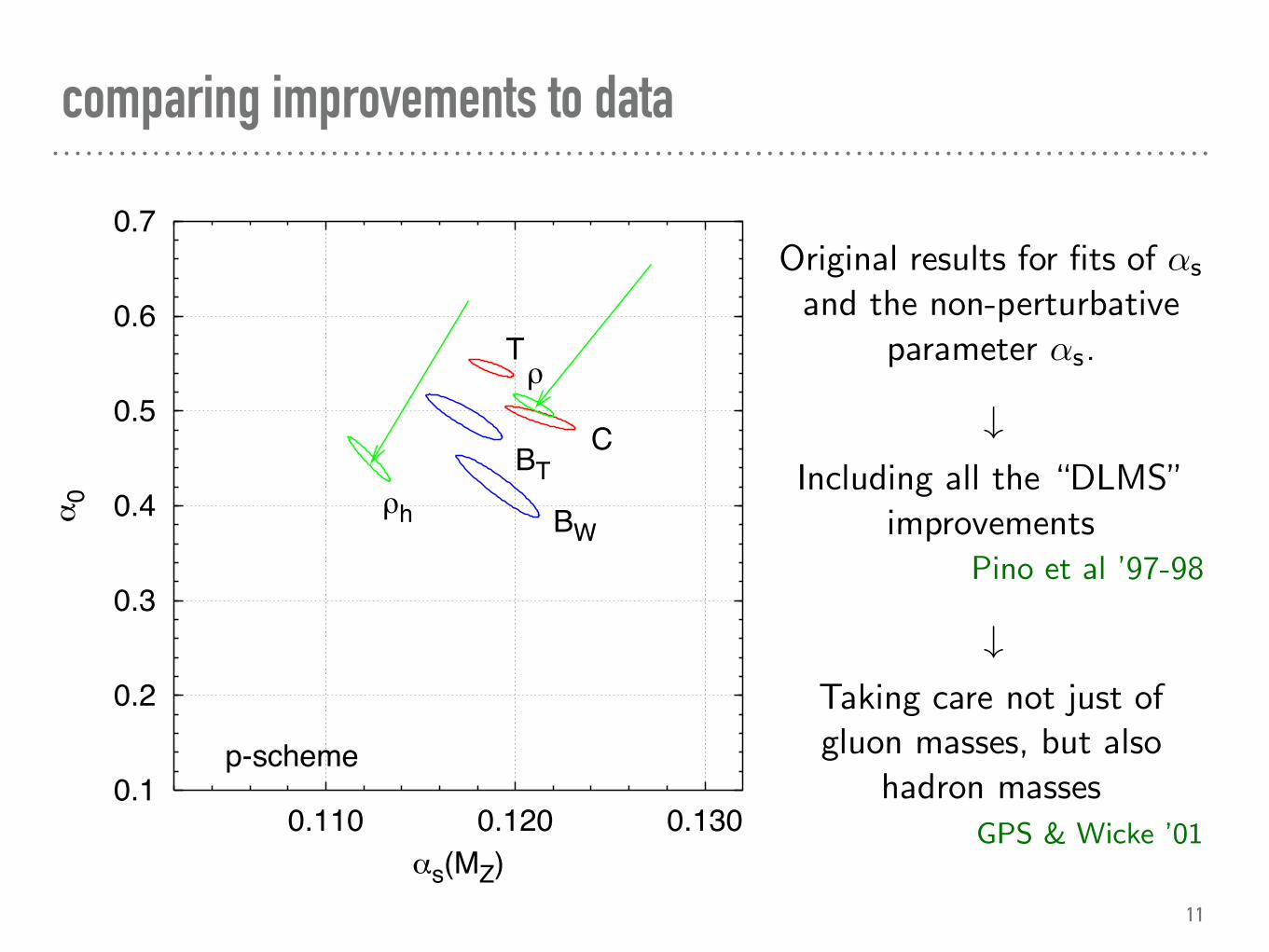
comparing improvements to data

9

0.1

0.2

0.3

0.4

0.5

0.6

0.7

0.110 0.120 0.130

α0

αs(MZ)

BW

BTC

T

ρhρ

Resummed coefficients



→


Pino et al ’97-98

→





10

0.1

0.2

0.3

0.4

0.5

0.6

0.7

0.110 0.120 0.130

α0

αs(MZ)

BW

BTC

T

ρh

ρ

p-scheme



→


Pino et al ’97-98

→





11

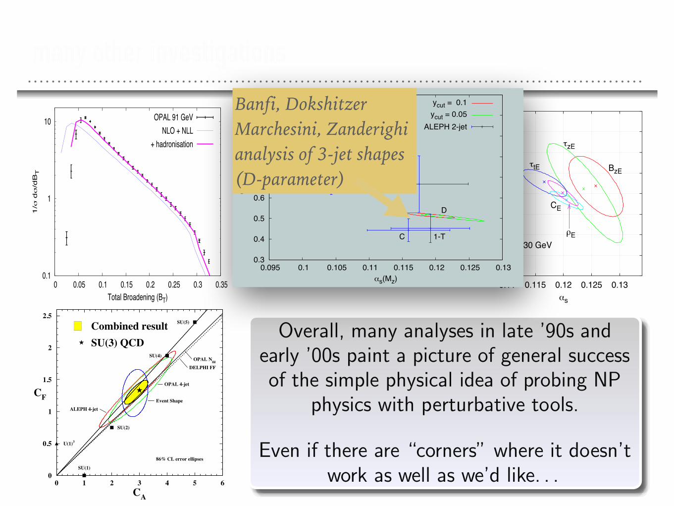
many other investigationsA rich field: many investigations in e+e− and DIS

0.1

1

10

0 0.05 0.1 0.15 0.2 0.25 0.3 0.35

1/σ

dσ

/dB

T

Total Broadening (BT)

OPAL 91 GeVNLO + NLL

+ hadronisation

0.4

0.5

0.6

0.7

0.8

0.9

0.08 0.1 0.12

average1-TMH, MH

2

BTBWC

α0

αS(MZ)

Distributions

a)

0.25

0.3

0.35

0.4

0.45

0.5

0.55

0.6

0.65

0.11 0.115 0.12 0.125 0.13

α0

αs

τtE

ρE

CE

τzE

BzE

Q > 30 GeV

(a)

0

0.5

1

1.5

2

2.5

0 1 2 3 4 5 6

U(1)3

SU(1)

SU(2)

SU(4)

SU(5)Combined resultSU(3) QCD

ALEPH 4-jet

OPAL 4-jet

Event Shape

OPAL Ngg

DELPHI FF

CF

CA

86% CL error ellipses

Overall, many analyses in late ’90s andearly ’00s paint a picture of general successof the simple physical idea of probing NP

physics with perturbative tools.

Even if there are “corners” where it doesn’twork as well as we’d like. . .


calculation obtained with nlojet++ [11], and leading 1/Q NP corrections computed withthe dispersive method [8, 9]. Events with three separated jets are selected by requiring thethree-jet resolution parameter y3 in the Durham algorithm to be larger than ycut. It is thenclear that different values of ycut correspond to different event geometries.

0.3

0.4

0.5

0.6

0.7

0.8

0.9

1

1.1

0.095 0.1 0.105 0.11 0.115 0.12 0.125 0.13

α0(

2GeV

)

αs(Mz)

1-T

MH

BT

BW

C

D

ycut = 0.1ycut = 0.05

ALEPH 2-jet

Figure 1: Contour plots in the αs-α0 planefor the D-parameter differential distributionscorresponding to two different values of ycut.

Figure 1 shows the result of a simultane-ous fit of αs(MZ) and α0(µI =2GeV) for theD-parameter distribution at Q = MZ cor-responding to ycut = 0.1 and ycut = 0.05.The 1-σ contour plots in the αs-α0 planeare plotted together with results for otherdistributions of two-jet event shapes. Thereis a remarkable consistency among the var-ious distributions, thus strongly supportingthe idea that universality of 1/Q power cor-rections holds also for three-jet variables.This leads to the non-trivial implicationthat leading power corrections are indeedsensitive to the colour and the geometryof the hard underlying event, and more-over this dependence is the one predictedby eq. (5).

0.001

0.01

0.1

1

10

100

1000

-2.4 -2.2 -2 -1.8 -1.6 -1.4 -1.2 -1 -0.8 -0.6

1/σ

dσ

/dL

L=ln(Tm)

ycut=0.1 (x 100)

ycut=0.05 (x 10)

ycut=0.025

NLO+NLL+1/QALEPH

Figure 2: Theoretical predictions for Tm dis-tribution plotted against ALEPH data forthree different values of ycut.

The comparison to data is less satisfac-tory for Tm, as can be seen from Fig. 2.There one notices a discrepancy betweentheory and data at large values of Tm. Totrack down the origin of the problem, onecan look at hadronisation corrections pro-duced by MC programs, defined as the ra-tio of the MC results at hadron and par-ton level. From the plots in [10] one cansee that hadronisation corrections for the D-parameter are always larger than one, corre-sponding to a positive shift, consistent withour predictions. On the contrary, hadro-nisation corrections for Tm become smallerthan one at large Tm, a feature that willnever be predicted by a model based on asingle dressed gluon emission from a threehard parton system. This issue is presentalso in the heavy-jet mass and wide-jet broadening distributions, and requires further theo-retical investigation.

3 Extension to other hard processes

Observables that measure the out-of-event-plane radiation in three-jet events can be intro-duced also in other hard processes.

In DIS two observables have been already measured. One is a variant of Tm [12], where

DIS 2007

Banfi, Dokshitzer Marchesini, Zanderighi analysis of 3-jet shapes (D-parameter)

NOW MOVE FORWARDS 15-20 YEARS

many NNLO calculations have become available (for e+e–, DIS and pp)

LHC physics is reaching high precision, not just for QCD physics, but also

e.g. today for “dark-matter” searches, & in the future for Higgs physics

NNLO hadron-collider calculations v. time

14

explosion of calculations in past 24 months

as of April 2017, let me know of omissions

indirect constraints on Hcc coupling

15

4

by CMS [66] show that the residual experimental sys-tematic uncertainty will be reduced to the level of a fewpercent at the HL-LHC. Therefore, it is natural to studythe prospects of the method in future scenarios assuminga reduced theory uncertainty given that this error maybecome the limiting factor.

In order to investigate the future prospects of ourmethod, we need a more precise assessment of the non-perturbative corrections to the pT,h distribution. To esti-mate these e↵ects, we used MG5aMC@NLO and POWHEG [67]showered with Pythia 8.2 and found that the correc-tions can reach up to 2% in the relevant pT,h region.This finding agrees with recent analytic studies of non-perturbative corrections to pT,h (see e.g. [68]). With im-proved perturbative calculations, a few-percent accuracyin this observable will therefore be reachable.

We study two benchmark cases. Our LHC Run II sce-nario employs 0.3 ab1 of integrated luminosity and as-sumes a systematic error of ±3% on the experimentalside and a total theoretical uncertainty of ±5%. Thismeans that we envision that the non-statistical uncer-tainties present at LHC Run I can be halved in thecoming years, which seems plausible. Our HL-LHC sce-nario instead uses 3 ab1 of data and foresees a reduc-tion of both systematic and theoretical errors by an-other factor of two, leading to uncertainties of ±1.5%and ±2.5%, respectively. The last scenario is illustrativeof the reach that can be achieved with improved the-ory uncertainties. Alternative theory scenarios are dis-cussed in the appendix. In both benchmarks, we employps = 13TeV and the PDF4LHC15 nnlo mc set [69–72],

consider the range pT 2 [0, 100]GeV in bins of 5GeV,and take into account h ! , h ! ZZ ! 4` andh ! WW ! 2`2`. We assume that future measure-ments will be centred around the SM predictions. Thesechannels sum to a branching ratio of 1.2%, but given thelarge amount of data the statistical errors per bin willbe at the ±2% (±1%) level in our LHC Run II (HL-LHC) scenario. We model the correlation matrix as inthe 8TeV case.

The results of our 2 fits are presented in Figure 3,showing the constraints in the c–b plane. The un-shaded contours refer to the LHC Run II scenario withthe dot-dashed (dotted) lines corresponding to 2 =2.3 (5.99). Analogously, the shaded contours with thesolid (dashed) lines refer to the HL-LHC. By profilingover b, we find in the LHC Run II scenario the follow-ing 95% CL bound on the yc modifications

c 2 [1.4, 3.8] (LHC Run II) , (3)

while the corresponding HL-LHC bound reads

c 2 [0.6, 3.0] (HL-LHC) . (4)

These limits compare well not only with the projectedreach of other proposed strategies but also have the nice

×

2 = 2.3 2 = 5.99

LHC Run II

HL-LHC

-6 -4 -2 0 2 4 6

-1

0

1

2

c

b

Figure 3: Projected future constraints in the c–b plane.The SM point is indicated by the black cross. The figureshows our projections for the LHC Run II (HL-LHC) with0.3 ab1 (3 ab1) of integrated luminosity at

ps = 13TeV.

The remaining assumptions entering our future predictionsare detailed in the main text.

feature that they are controlled by the size of systematicuncertainties that can be reached in the future. Also, atfuture LHC runs our method will allow one to set relevantbounds on the modifications of yb. For instance, in theHL-HLC scenario we obtain b 2 [0.7, 1.6] at 95% CL.Finally, we also explored the possibility of constrain-

ing modifications of the strange Yukawa coupling. Underthe assumption that yb is SM-like but profiling over c,we find that at the HL-LHC one should have a sensitiv-ity to ys values of around 30 times the SM expectation.Measurements of exclusive h ! decays are expectedto have a reach that is weaker than this by a factor oforder 100 [11].Conclusions. In this letter, we have demonstrated

that the normalised pT distribution of the Higgs or ofjets recoiling against it, provide sensitive probes of thebottom, charm and strange Yukawa couplings. Our newproposal takes advantage of the fact that the di↵eren-tial Higgs plus jets cross section receives contributionsfrom the channels gg ! hj, gQ ! hQ, QQ ! hgthat feature two di↵erent functional dependences on Q.We have shown that in the kinematic region where thetransverse momentum p

?

of emissions is larger than therelevant quark mass mQ, but smaller than the Higgsmass mh, both e↵ects can be phenomenologically rele-vant and thus their interplay results in an enhanced sen-sitivity to Q. This feature allows one to obtain uniqueconstraints on yb, yc and ys at future LHC runs.We derived constraints in the c–b plane that arise

from LHC Run I data and provided sensitivity projec-

2

momenta pT . mh/2. This partly compensates for thequadratic mass suppression m2

Q/m2h appearing in (1). As

a result of the logarithmic sensitivity and of the 2Q de-

pendence in quark-initiated production, one expects de-viations of several percent in the pT spectra in Higgsproduction for O(1) modifications of Q. In the SM,the light-quark e↵ects are small. Specifically, in compar-ison to the Higgs e↵ective field theory (HEFT) predic-tion, in gg ! hj the bottom contribution has an e↵ectof around 5% on the di↵erential distributions while theimpact of the charm quark is at the level of 1%. Like-wise, the combined gQ ! hQ, QQ ! hg channels (withQ = b, c) lead to a shift of roughly 2%. Precision mea-surements of the Higgs distributions for moderate pTvalues combined with precision calculations of these ob-servables are thus needed to probe O(1) deviations in yband yc. Achieving such an accuracy is both a theoreticaland experimental challenge, but it seems possible in viewof foreseen advances in higher-order calculations and thelarge statistics expected at future LHC runs.

Theoretical framework. Our goal is to explorethe sensitivity of the Higgs-boson (pT,h) and leading-jet (pT,j) transverse momentum distributions in inclusiveHiggs production to simultaneous modifications of thelight Yukawa couplings. We consider final states wherethe Higgs boson decays into a pair of gauge bosons. Toavoid sensitivity to the modification of the branching ra-tios, we normalise the distributions to the inclusive crosssection. The e↵ect on branching ratios can be included inthe context of a global analysis, jointly with the methodproposed here.

The gg ! hj channel was analysed in depth in theHEFT framework where one integrates out the domi-nant top-quark loops and neglects the contributions fromlighter quarks. While in this approximation the twospectra and the total cross section were studied exten-sively, the e↵ect of lighter quarks is not yet known withthe same precision for pT . mh/2. Within the SM,the LO distribution for this process was derived longago [17, 19], and the next-to-leading-order (NLO) cor-rections to the total cross section were calculated in [20–24]. In the context of analytic resummations of the Su-dakov logarithms ln (pT /mh), the inclusion of mass cor-rections to the HEFT were studied both for the pT,h

and pT,j distributions [25–27]. More recently, the firstresummations of some of the leading logarithms (1) wereaccomplished both in the abelian [28] and in the high-energy [29] limit. The reactions gQ ! hQ, QQ ! hgwere computed at NLO [30, 31] in the five-flavour schemethat we employ here, and the resummation of the loga-rithms ln (pT,h/mh) in QQ ! h was also performed up tonext-to-next-to-leading-logarithmic (NNLL) order [32].

In the case of gg ! hj, we generate the LO spectrawith MG5aMC@NLO [33]. We also include NLO correctionsto the spectrum in the HEFT [34–36] using MCFM [37].The total cross sections for inclusive Higgs production

0 20 40 60 80 100

0.8

1.0

1.2

1.4

pT,h [GeV]

(1/

d/d

pT

,h)/(1/

d/d

pT

,h) S

M

c = -10

c = -5

c = 0

c = 5

Figure 1: The normalised pT,h spectrum of inclusive Higgsproduction at

ps = 8TeV divided by the SM prediction for

di↵erent values of c. Only c is modified, while the remain-ing Yukawa couplings are kept at their SM values.

are obtained from HIGLU [38], taking into account theNNLO corrections in the HEFT [39–41]. Sudakov loga-rithms ln (pT /mh) are resummed up to NNLL order bothfor pT,h [42–44] and pT,j [45–47], treating mass correc-tions following [27]. The latter e↵ects will be significant,once the spectra have been precisely measured down topT values of O(5GeV). The gQ ! hQ, QQ ! hg contri-butions to the distributions are calculated at NLO withMG5aMC@NLO [48] and cross-checked against MCFM. The ob-tained events are showered with PYTHIA 8.2 [49] and jetsare reconstructed with the anti-kt algorithm [50] as im-plemented in FastJet [51] using R = 0.4 as a radiusparameter.Our default choice for the renormalisation (µR), fac-

torisation (µF ) and the resummation (QR, for gg ! hj)scales is mh/2. Perturbative uncertainties are estimatedby varying µR, µF by a factor of two in either direc-tion while keeping 1/2 µR/µF 2. In addition, forthe gg ! hj channel, we vary QR by a factor of twowhile keeping µR = µF = mh/2. The final total theo-retical errors are then obtained by combining the scaleuncertainties in quadrature with a ±2% relative error as-sociated with PDFs and ↵s for the normalised distribu-tions. We stress that the normalised distributions usedin this study are less sensitive to PDFs and ↵s varia-tions, therefore the above ±2% relative uncertainty is arealistic estimate. We obtain the relative uncertainty inthe SM and then assume that it does not depend on Q.While this is correct for the gQ ! hQ, QQ ! hg chan-nels, for the gg ! hj production a good assessment ofthe theory uncertainties in the large-Q regime requiresthe resummation of the logarithms in (1). First steps in

impact of modified Hcc coupling on Higgs+jet pT

joint limits on κc & κb @ HL-LHC

Fady Bishara, Ulrich Haisch, Pier Francesco Monni and Emanuele Re, arXiv:1606.09253 see also Y. Soreq, H. X. Zhu, and J. Zupan, JHEP 12, 045 (2016), 1606.09621

Extracting αs from e+e- event shapes and jet rates Two “best” determinations are from same group

(Hoang et al, 1006.3080,1501.04111)αs(MZ) = 0.1135 ± 0.0010 (0.9%) [thrust] αs(MZ) = 0.1123 ± 0.0015 (1.3%) [C-parameter]

Similar result from Gehrmann, Luisoni & Monni (1210.6945)αs(MZ) = 0.1131 ± 0.0028 (2.5%) [thrust]

lattice:αs(MZ) = 0.1183 ± 0.0007 (0.6%) [HPQCD]αs(MZ) = 0.1186 ± 0.0008 (0.7%) [ALPHA prelim.]

36 1. Quantum chromodynamics

τ-decays

latticestru

cture

fun

ction

se+

e- an

nih

ilation

hadron collider

electroweakprecision fits

Baikov

ABMBBGJR

MMHT

NNPDF

Davier

PichBoitoSM review

HPQCD (Wilson loops)

HPQCD (c-c correlators)

Maltmann (Wilson loops)

JLQCD (Adler functions)

Dissertori (3j)

JADE (3j)

DW (T)

Abbate (T)

Gehrm. (T)

CMS (tt cross section)

GFitter

Hoang (C)

JADE(j&s)

OPAL(j&s)

ALEPH (jets&shapes)

PACS-CS (vac. pol. fctns.)

ETM (ghost-gluon vertex)

BBGPSV (static energy)

Figure 1.2: Summary of determinations of αs(M2Z) from the six sub-fields

discussed in the text. The yellow (light shaded) bands and dashed lines indicate thepre-average values of each sub-field. The dotted line and grey (dark shaded) bandrepresent the final world average value of αs(M2

Z).

So far, only one analysis is available which involves the determination of αs fromhadron collider data in NNLO of QCD: from a measurement of the tt cross section at

February 22, 2016 10:28


τ-decays

latticestru

cture

fun

ction

se+

e- an

nih

ilation

hadron collider


Baikov

ABMBBGJR

MMHT

NNPDF

Davier

PichBoitoSM review




JLQCD (Adler functions)

Dissertori (3j)

JADE (3j)

DW (T)

Abbate (T)

Gehrm. (T)


GFitter

Hoang (C)

JADE(j&s)

OPAL(j&s)

ALEPH (jets&shapes)

PACS-CS (vac. pol. fctns.)


BBGPSV (static energy)



Z).

So far, only one analysis is available which involves the determination of αs fromhadron collider data in NNLO of QCD: from a measurement of the tt cross section at

February 22, 2016 10:28


τ-decays

latticestru

cture

fun

ction

se

+e–

jets & sh

apes

hadron collider


Baikov

ABMBBGJR

MMHT

NNPDF

Davier

PichBoitoSM review




Dissertori (3j)

JADE (3j)

DW (T)

Abbate (T)

Gehrm. (T)


GFitter

Hoang (C)

JADE(j&s)

OPAL(j&s)

ALEPH (jets&shapes)

PACS-CS (SF scheme)


BBGPSV (static potent.)

April 2016



Z).

using the transverse energy-energy correlation function (TEEC) and its associatedazimuthal asymmetry (ATEEC), respectively [247]. All these results are at NLO only,however they provide valuable new values of αs at energy scales now extending up to

May 5, 2016 21:57

thrust & “best” lattice are 4-σ apart

Comments:

thrust & C-parameter are highly correlated observables

Analysis valid far from 3-jet region, but not too deep into 2-jet region — at LEP, not clear how much of distribution satisfies this requirement

thrust fit shows noticeable sensitivity to fit region (C-parameter doesn't)

30

!"### !"##$ !"##% !"##& !"##' !"##(!"&!

!"'!

!"(!

!")!

!"*!!"

+*H9/

0PLQ PD[

8

Q0 250 "

VWULFW

8

Q0 330 "

VWULFW

vary 0 330

5

Q0 380 "

5

Q0 330

6

Q0 380 "

6

Q0 250

VWULFW

6

Q0 330

VWULFW

0 330 "0 09"

8

Q0 330

:ELQV

&*)

&%%%<$

'&'

'#(

')&

&$)

%%'

&&$

%<&

"

"

"

"

"

39% CL

68% CL

τ τ

FIG. 17: The smaller elongated ellipses show the experimental39% CL error (1-sigma for αs) and best fit points for differentglobal data sets at N3LL′ order in the R-gap scheme andincluding bottom quark mass and QED effects. The defaulttheory parameters given in Tab. III are employed. The largerellipses show the combined theoretical plus experimental errorfor our default data set with 39% CL (solid, 1-sigma for onedimension) and 68% CL (dashed).

experimental error ellipses, hence to larger uncertainties.It is an interesting but expected outcome of the fits

that the pure experimental error for αs (the uncertaintyof αs for fixed central Ω1) depends fairly weakly on theτ range and the size of the global data sets shown inFig. 17. If we had a perfect theory description then wewould expect that the centers and the sizes of the errorellipses would be statistically compatible. Here this isnot the case, and one should interpret the spread of theellipses shown in Fig. 17 as being related to the theo-retical uncertainty contained in our N3LL′ order predic-tions. In Fig. 17 we have also displayed the combined(experimental and theoretical) 39% CL standard errorellipse from our default global data set which was al-ready shown in Fig. 11a (and is 1-sigma, 68% CL, foreither one dimensional projection). We also show the68% CL error ellipse by a dashed red line, which corre-sponds to 1-sigma knowledge for both parameters. Aswe have shown above, the error in both the dashed andsolid larger ellipses is dominated by the theory scan un-certainties, see Eqs. (68). The spread of the error ellipsesfrom the different global data sets is compatible with the1-sigma interpretation of our theoretical error estimate,and hence is already represented in our final results.

Analysis without Power Corrections

Using the simple assumption that the thrust distributionin the tail region is proportional to αs and that the main

αs(mZ)±(pert. error) χ2/(dof)

N3LL′ with ΩRgap1 0.1135 ± 0.0009 0.91

N3LL′ with ΩMS1 0.1146 ± 0.0021 1.00

N3LL′ without Smodτ 0.1241 ± 0.0034 1.26

O(α3s) fixed-order

without Smodτ

0.1295 ± 0.0046 1.12

TABLE VII: Comparison of global fit results for our full anal-ysis to a fit where the renormalon is not canceled with Ω1, afit without Smod

τ (meaning without power corrections withSmodτ (k) = δ(k)), and a fit at fixed order without power cor-

rections and log resummation. All results include bottommass and QED corrections.

effect of power corrections is a shift of the distributionin τ , we have estimated in Sec. I that a 300MeV powercorrection will lead to an extraction of αs from Q = mZ

data that is δαs/αs ≃ (−9 ± 3)% lower than an anal-ysis without power corrections. In our theory code wecan easily eliminate all nonperturbative effects by set-ting Smod

τ (k) = δ(k) and ∆ = δ = 0. At N3LL′ or-der and using our scan method to determine the per-turbative uncertainty a global fit to our default data setyields αs(mZ) = 0.1241 ± (0.0034)pert which is indeed9% larger than our main result in Eq. (68) which ac-counts for nonperturbative effects. It is also interestingto do the same fit with a purely fixed-order code, whichwe can do by setting µS = µJ = µH to eliminate thesummation of logarithms. The corresponding fit yieldsαs(mZ) = 0.1295±(0.0046)pert, where the displayed errorhas again been determined from the theory scan which inthis case accounts for variations of µH and the numericaluncertainties associated with ϵ2 and ϵ3. (A comparisonwith Ref. [22] is given below in Sec. IX.)These results have been collected in Tab. VII together

with the αs results of our analyses with power correctionsin the R-gap and the MS schemes. For completeness wehave also displayed the respective χ2/dof values whichwere determined by the average of the maximal and theminimum values obtained in the scan.

VIII. FAR-TAIL AND PEAK PREDICTIONS

The factorization formula (4) can be simultaneously usedin the peak, tail, and far-tail regions. To conclude thediscussion of the numerical results of our global analysisin the tail region, we use the results obtained from thistail fit to make predictions in the peak and the far-tailregions.In Fig. 18 we compare predictions from our full N3LL′

code in the R-gap scheme (solid red line) to the accurateALEPH data at Q = mZ in the far-tail region. As inputfor αs(mZ) and Ω1 we use our main result of Eq. (68)and all other theory parameters are set to their defaultvalues (see Tab. III). We find excellent agreement withinthe theoretical uncertainties (pink band). Key features

dependence on fit range

16

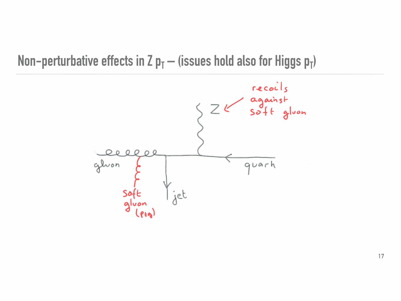
Non-perturbative effects in Z pT – (issues hold also for Higgs pT)

17

Non-perturbative effects in Z pT

18


19

A conceptually similar problem is present for the W momentum in top decays


impact of 0.5 GeV shift of Z pT

0.5 GeV is perhaps conservative(?)

Inclusive Z cross section should have ~Λ2/M2 corrections (~10-4 ?)

Z pT is not inclusive so corrections can be ~Λ/M.

Size of effect can’t be probed by turning MC hadronisation on/off[maybe by modifying underlying MC parameters?]

Shifting Z pT by a finite amount illustrates what could happen

20

Closing remarks

This is just one of several fun physics topicsthat were pushed forwards in the late ’90s

with Pino in Milan.small x , resummations were others

Pino wrote ∼ 15 articles with the studentsand postdocs then

(including Banfi, Dasgupta, GPS, Smye,Zanderighi)

Many of the collaborations that formedbetween them then have continued to thisday, easily having produced another ∼ 15

articles.


X24

21

EXTRAS

22

LHC PRECISION: PERTURBATION THEORY

Lindert, Pozzorini et al, 1705.04664

±2%

Z(`+`)+ jet

W(`n)+ jet

W+(`+n)+ jet

g+ jet

10 x W(`n)+ jet

100 x W+(`+n)+ jet

Z(`+`)+ jet

1000 x g+ jet

NLO QCD nNLO EWNNLO QCD nNLO EWPDF Uncertanties (LUXqed)

1010109108107106105104103102101

110 110 210 310 410 5

V+jet @ 13 TeV

ds

/dp T

,V[p

b/G

eV]

0.80.85

0.90.95

1.01.05

1.11.15

1.2

ds

/ds N

LO

QC

D

0.80.85

0.90.95

1.01.05

1.11.15

1.2

ds

/ds N

LO

QC

D

0.80.85

0.90.95

1.01.05

1.11.15

1.2

ds

/ds N

LO

QC

D

100 200 500 1000 3000

0.80.85

0.90.95

1.01.05

1.11.15

1.2

pT,V [GeV]

ds

/ds N

LO

QC

D

Z(`+`) / W(`n)

Z(`+`) / g

W(`n) / W+(`+n)Z(`+`) / Z(nn)

W(`n) / W+(`+n)

Z(`+`) / g

Z(`+`) / W(`n)

Z(`+`) / Z(nn)


102

101

1

V+jet ratios @ 13 TeV

R

0.9

0.95

1.0

1.05

1.1

R/

RQ

CDE

W

0.9

0.95

1.0

1.05

1.1

R/

RQ

CDE

W0.9

0.95

1.0

1.05

1.1

R/

RQ

CDE

W

100 200 500 1000 3000

0.9

0.95

1.0

1.05

1.1

pT,V [GeV]

R/

RQ

CDE

W

Figure 17: Predictions at NLO QCD nNLO EW and NNLO QCD nNLO EW for V+ jetspectra (left) and ratios (right) at 13 TeV. The lower frames show the relative impact ofNNLO corrections and theory uncertainties normalised to NLO QCD nNLO EW. Thegreen bands at NLO QCD nNLO EW correspond to the combination (in quadrature)of the perturbative QCD, EW and mixed QCD-EW uncertainties, according to Eq. (45),while the NNLO QCD nNLO EW bands (red) display only QCD scale variations. PDFuncertainties are shown as separate hashed orange bands.

based on NLO QCD. PDF uncertainties are below the perturbative uncertainties in allnominal distributions and all but the W/W+ ratio. Clearly, a precise measurement ofthe W/W+ ratio at high pT, where perturbative uncertainties almost completely cancel,will help to improve PDF fits.

Our predictions are provided in the form of tables for the central predictions and forthe different uncertainty sources. Each uncertainty source is to be treated as a 1-standarddeviation uncertainty and pragmatically associated with a Gaussian-distributed nuisanceparameter.

The predictions are given at parton level as distributions of the vector boson pT, withloose cuts and inclusively over other radiation. They are intended to be propagated to anexperimental analysis using Monte Carlo parton shower samples whose inclusive vector-boson pT distribution has been reweighted to agree with our parton-level predictions. Theimpact of additional cuts, non-perturbative effects on lepton isolation, etc., can then bededuced from the Monte Carlo samples. The additional uncertainties associated with the

35

Z(`+`)+ jet

W(`n)+ jet

W+(`+n)+ jet

g+ jet

10 x W(`n)+ jet

100 x W+(`+n)+ jet

Z(`+`)+ jet

1000 x g+ jet


1010109108107106105104103102101

110 110 210 310 410 5

V+jet @ 13 TeV

ds

/dp T

,V[p

b/G

eV]

0.80.85

0.90.95

1.01.05

1.11.15

1.2

ds

/ds N

LO

QC

D

0.80.85

0.90.95

1.01.05

1.11.15

1.2

ds

/ds N

LO

QC

D0.8

0.850.9

0.951.0

1.051.1

1.151.2

ds

/ds N

LO

QC

D

100 200 500 1000 3000

0.80.85

0.90.95

1.01.05

1.11.15

1.2

pT,V [GeV]

ds

/ds N

LO

QC

D

Z(`+`) / W(`n)

Z(`+`) / g

W(`n) / W+(`+n)Z(`+`) / Z(nn)

W(`n) / W+(`+n)

Z(`+`) / g

Z(`+`) / W(`n)

Z(`+`) / Z(nn)


102

101

1

V+jet ratios @ 13 TeV

R

0.9

0.95

1.0

1.05

1.1

R/

RQ

CDE

W

0.9

0.95

1.0

1.05

1.1

R/

RQ

CDE

W

0.9

0.95

1.0

1.05

1.1

R/

RQ

CDE

W

100 200 500 1000 3000

0.9

0.95

1.0

1.05

1.1

pT,V [GeV]

R/

RQ

CDE

W

Figure 17: Predictions at NLO QCD nNLO EW and NNLO QCD nNLO EW for V+ jetspectra (left) and ratios (right) at 13 TeV. The lower frames show the relative impact ofNNLO corrections and theory uncertainties normalised to NLO QCD nNLO EW. Thegreen bands at NLO QCD nNLO EW correspond to the combination (in quadrature)of the perturbative QCD, EW and mixed QCD-EW uncertainties, according to Eq. (45),while the NNLO QCD nNLO EW bands (red) display only QCD scale variations. PDFuncertainties are shown as separate hashed orange bands.

based on NLO QCD. PDF uncertainties are below the perturbative uncertainties in allnominal distributions and all but the W/W+ ratio. Clearly, a precise measurement ofthe W/W+ ratio at high pT, where perturbative uncertainties almost completely cancel,will help to improve PDF fits.

Our predictions are provided in the form of tables for the central predictions and forthe different uncertainty sources. Each uncertainty source is to be treated as a 1-standarddeviation uncertainty and pragmatically associated with a Gaussian-distributed nuisanceparameter.

The predictions are given at parton level as distributions of the vector boson pT, withloose cuts and inclusively over other radiation. They are intended to be propagated to anexperimental analysis using Monte Carlo parton shower samples whose inclusive vector-boson pT distribution has been reweighted to agree with our parton-level predictions. Theimpact of additional cuts, non-perturbative effects on lepton isolation, etc., can then bededuced from the Monte Carlo samples. The additional uncertainties associated with the

35

23

Z+jet process is main background for LHC dark-matter searches.

And powerful input for PDF fits.

Perturbative results are very precise…

LHC PRECISION: EXPERIMENT

[GeV]llT

p

100

]σ

Pull

[

2−02

50 500

210

Com

bine

dC

hann

el

0.80.9

11.11.2

/NDF= 8/82χ

210

]-1 [

GeV

ll T/d

pσ

dσ

1/

5−10

4−10

3−10

2−10

1−10

ee-channel-channelµµ

CombinedStatistical uncertaintyTotal uncertainty

ATLAS| < 2.4

ll < 20 GeV, |yll m≤12 GeV

-1=8 TeV, 20.3 fbs

[GeV]llT

p

100

]σ

Pull

[

2−02

50 500

210

Com

bine

dC

hann

el

0.9

1

1.1

/NDF= 6/82χ

210

]-1 [

GeV

ll T/d

pσ

dσ

1/

5−10

4−10

3−10

2−10

1−10



ATLAS| < 2.4


-1=8 TeV, 20.3 fbs

[GeV]llT

p

100

]σ

Pull

[2−02

50 500

210C

ombi

ned

Cha

nnel

0.9

1

1.1

/NDF= 7/82χ

210

]-1 [

GeV

ll T/d

pσ

dσ

1/

5−10

4−10

3−10

2−10

1−10



ATLAS| < 2.4


-1=8 TeV, 20.3 fbs

[GeV]llT

p1 10 210

]σ

Pull

[

2−02 1 10 210

Com

bine

dC

hann

el

0.95

1

1.05

/NDF=13/202χ

1 10 210

]-1 [

GeV

ll T/d

pσ

dσ

1/

6−10

5−10

4−10

3−10

2−10

1−10

1



ATLAS -1=8 TeV, 20.3 fbs| < 2.4


[GeV]llT

p1 10 210

]σ

Pull

[

2−02 1 10 210

Com

bine

dC

hann

el

0.99

1

1.01

/NDF=43/432χ

1 10 210

]-1 [

GeV

ll T/d

pσ

dσ

1/

8−10

7−10

6−10

5−10

4−10

3−10

2−10

1−101



ATLAS -1=8 TeV, 20.3 fbs| < 2.4


[GeV]llT

p1 10 210

]σ

Pull

[2−02 1 10 210

Com

bine

dC

hann

el

0.95

1

1.05

/NDF=27/202χ

1 10 210

]-1 [

GeV

ll T/d

pσ

dσ

1/

5−10

4−10

3−10

2−10

1−10

1



ATLAS -1=8 TeV, 20.3 fbs| < 2.4


Figure 6: The Born-level distributions of (1/) d/dp``T for the combination of the electron-pair and muon-pairchannels, shown in six m`` regions for |y`` | < 2.4. The central panel of each plot shows the ratios of the values fromthe individual channels to the combined values, where the error bars on the individual-channel measurements rep-resent the total uncertainty uncorrelated between bins. The light-blue band represents the data statistical uncertaintyon the combined value and the dark-blue band represents the total uncertainty (statistical and systematic). The 2

per degree of freedom is given. The lower panel of each plot shows the pull, defined as the di↵erence between theelectron-pair and muon-pair values divided by the uncertainty on that di↵erence.

18

±1%

24

Experimental results are equally precise.

REMARKS

Non-pert. effects are always relevant at accuracies we’re interested in

Watch out for cancellation between “hadronisation” and MPI/UE (separate physical effects)

Definition of perturbative / non-perturbative is ambiguous

Alternative to MC: analytical estimates.MC’s have strong pT dependence, missing in analytical estimates

-0.6

-0.5

-0.4

-0.3

-0.2

-0.1

0

0.1

200 500 100 1000

pp, 7 TeV, no UE

Δpth

adr ×

R C

F/C

[G

eV

]

pt (parton) [GeV]

hadronisation pt shift (scaled by R CF/C)

Herwig 6 (AUET2)

Pythia 8 (Monash 13)

R=0.2, quarks

R=0.4, quarks

R=0.2, gluons

R=0.4, gluons

Monte Carlo tune jet radius, flavour

simple analytical estimate

Figure 11. The average shift in jet pt induced by hadronisation in a range of Monte Carlo tunes,for R = 0.4 and R = 0.2 jets, both quark and gluon induced. The shift is shown as a function ofjet pt and is rescaled by a factor RCF /C (C = CF or CA) in order to test the scaling expectedfrom Eq. (5.1). The left-hand plot shows results from the AUET2 [48] tune of Herwig 6.521 [22, 23]and the Monash 13 tune [49] of Pythia 8.186 [21], while the right-hand plot shows results fromthe Z2 [50] and Perugia 2011 [51, 52] tunes of Pythia 6.428 [20]. The shifts have been obtainedby clustering each Monte Carlo event at both parton and hadron level, matching the two hardestjets in the two levels and determining the di↵erence in their pt’s. The simple analytical estimate of0.5GeV ± 20% is shown as a yellow band.

and Pythia 8 Monash 2013 both having somewhat smaller than expected hadronisation

corrections. Secondly there is a strong dependence of the shift on the initial jet pt, with

a variation of roughly a factor of two between pt = 100GeV and pt = 1TeV. Such a ptdependence is not predicted within simple approaches to hadronisation such as Refs. [19,

43, 46, 47]. It was not observed in Ref. [19] because the Monte Carlo study there restricted

its attention to a limited range of jet pt, 55 70GeV. The event shape studies that

provided support for the analytical hadronisation were also limited in the range of scales

they probed, specifically, centre-of-mass energies in the range 40200GeV (and comparable

photon virtualities in DIS). Note, however, that scale dependence of the hadronisation has

been observed at least once before, in a Monte Carlo study shown in Fig. 8 of Ref. [53]:

e↵ects found there to be associated with hadron masses generated precisely the trend seen

here in Fig. 11. The pt dependence of those e↵ects can be understood analytically, however

we leave their detailed study in a hadron-collider context to future work.13 Experimental

insight into the pt dependence of hadronisation might be possible by examining jet-shape

measurements [55, 56] over a range of pt, however such a study is also beyond the scope of

this work.

In addition to the issues of pt dependence, one further concern regarding the analytical

approach is that it has limited predictive power for the fluctuations of the hadronisation

13Hadron-mass e↵ects have been discussed also in the context of Ref. [54].

– 20 –

25

Analytic v. MC hadronisation

non-perturbative effects may become a key limitation at 1%

STANDARD MODEL TODAY

KNOWLEDGEASSUMPTION

Gauge interactions well tested.

Higgs sector mostly an assumption

26

STANDARD MODEL TODAY

KNOWLEDGEASSUMPTION



t b τc s μu s e

27

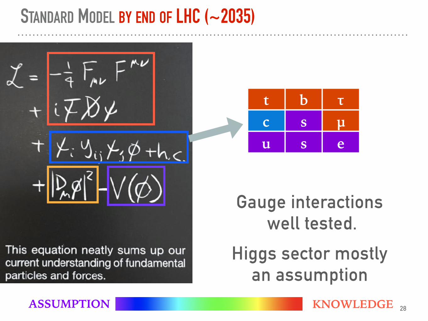
STANDARD MODEL BY END OF LHC (~2035)

KNOWLEDGEASSUMPTION



t b τc s μu s e

28

N3LO

29

Figure 2: E↵ective theory production cross section of a scalar particle of mass mS 2 [50, 150] GeVthrough increasing orders in perturbation theory. For further details see the caption of Fig. 1.

mass around 770 GeV. This feature is not shared with individual PDF sets. We therefore

use, conservatively, the envelope of CT14, NNPDF30 and PDF4LHC, which leads to an

uncertainty due to the lack of N3LO parton densities at the level of 0.9% 3% for scalars

in the range 50 GeV3 TeV. This uncertainty remains of the order of a few percent also

at lower masses, but it increases rapidly to O(10%) for mS . 20 GeV.

We present the cross section values and uncertainties for this range of scalar masses in

Appendix A. In particular, in Tab. 6 we focus on the range between 730 and 770 GeV.

3. Finite width e↵ects and the line-shape

The results of the previous section hold formally only when the width of the scalar is set to

zero. In many beyond the Standard Model (BSM) scenarios, however, finite-width e↵ects

cannot be neglected. In this section we present a way to include leading finite-width e↵ects

into our results, in the case where the width is not too large compared to the mass.

The total cross section for the production of a scalar boson of total width S can be

obtained from the cross section in the zero-width approximation via a convolution

S(mS ,S ,UV) =

ZdQ2QS(Q)

S(Q,S = 0,UV)

(Q2 m2S)

2 +m2S

2(mS)+O (S(mS)/mS) , (3.1)

where Q is the virtuality of the scalar particle. This expression is accurate at leading order

in S(mS)/mS . For large values of the width relative to the mass, subleading corrections

– 6 –

4

1

10

100PDF4LHC15_nnlo_mcQ/2 < µR , µF < 2 Q

[pb]

LONLO

NNLON3LO

0.99

1

1.01

1.02

7 13 20 30 50 10 100

rati

o to

N3L

O

s [TeV]

10-4

10-3

10-2

10-1

PDF4LHC15_nnlo_mcQ/2 < µR , µF < 2 QLHC 13 TeV

d/dpt,H [pb/GeV]

LONLO

NNLON3LO

0.99

1

1.01

1.02

0 50 100 150 200 250 300

pt,H [GeV]

FIG. 4. Cross section as a function of center-of-mass energy (left), Higgs transverse momentum distribution (center) and Higgsrapidity distribution (right).

(13 TeV) [pb] (14 TeV) [pb] (100 TeV) [pb]

LO 4.099+0.0510.067 4.647+0.037

0.058 77.17+6.457.29

NLO 3.970+0.0250.023 4.497+0.032

0.027 73.90+1.731.94

NNLO 3.932+0.0150.010 4.452+0.018

0.012 72.44+0.530.40

N3LO 3.928+0.0050.001 4.448+0.006

0.001 72.34+0.110.02

TABLE I. Inclusive cross sections at LO, NLO, NNLO andN3LO for VBF Higgs production. The quoted uncertaintiescorrespond to scale variations Q/2 < µR, µF < 2Q, whilestatistical uncertainties are at the level of 0.2h.

order in QCD, where we observe again a large reductionof the theoretical uncertainty at N3LO.

A comment is due on non-factorisable QCD correc-tions. Indeed, for the results presented in this letter, wehave considered VBF in the usual DIS picture, ignor-ing diagrams that are not of the type shown in figure 1.These e↵ects neglected by the structure function approx-imation are known to contribute less than 1% to the totalcross section at NNLO [7]. The e↵ects and their relativecorrections are as follows:

• Gluon exchanges between the upper and lower ha-dronic sectors, which appear at NNLO, but arekinematically and colour suppressed. These contri-butions along with the heavy-quark loop inducedcontributions have been estimated to contribute atthe permille level [7].

• t-/u-channel interferences which are known to con-tribute O(5h) at the fully inclusive level andO(0.5h) after VBF cuts have been applied [10].

• Contributions from s-channel production, whichhave been calculated up to NLO [10]. At the inclu-sive level these contributions are sizeable but theyare reduced to O(5h) after VBF cuts.

• Single-quark line contributions, which contribute tothe VBF cross section at NNLO. At the fully inclu-sive level these amount to corrections of O(1%) butare reduced to the permille level after VBF cutshave been applied [11].

• Loop induced interferences between VBF andgluon-fusion Higgs production. These contribu-tions have been shown to be much below the per-mille level [36].

Furthermore, for phenomenological applications, onealso needs to consider NLO electroweak e↵ects [10], whichamount to O(5%) of the total cross section. We leave adetailed study of non-factorisable and electroweak e↵ectsfor future work. The code used for this calculation willbe published in the near future [37].In this letter, we have presented the first N3LO calcula-

tion of a 2 ! 3 hadron-collider process, made possible bythe DIS-like factorisation of the process. This brings theprecision of VBF Higgs production to the same formal ac-curacy as was recently achieved in the gluon-gluon fusionchannel in the heavy top mass approximation [12]. The

N3LO ggF Higgs N3LO VBF Higgs

Anastasiou et al, 1602.00695 Dreyer & Karlberg, 1606.00840

N3LO

NNLO N3LO

NNLO

WH at large Q2 with dim-6 BSM effect

3000 fb-1

schemati

new physics isn’t just a single

number that’s wrong (think g-2)

but rather a distinct scaling

pattern of deviation (~ pT2)

moderate and high pT’s have similar

statistical significance — so

it’s useful to understand whole

pT range

GPS 2016-10

30

Documents

POWER CORRECTIONS FROM MILAN TO LHC