Class 8: Radiometric Corrections

Sensor CorrectionsAtmospheric Corrections

Conversion from DN to reflectanceBRDF Corrections

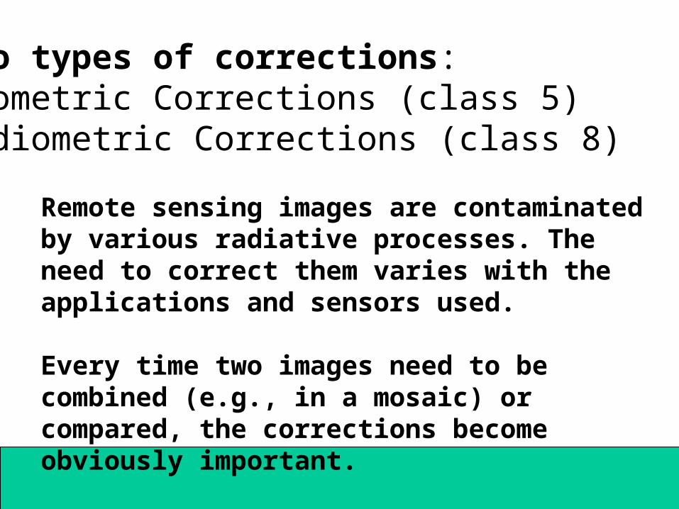
Remote sensing images are contaminated by various radiative processes. The need to correct them varies with the applications and sensors used.

Every time two images need to be combined (e.g., in a mosaic) or compared, the corrections become obviously important.

Two types of corrections:Geometric Corrections (class 5)Radiometric Corrections (class 8)

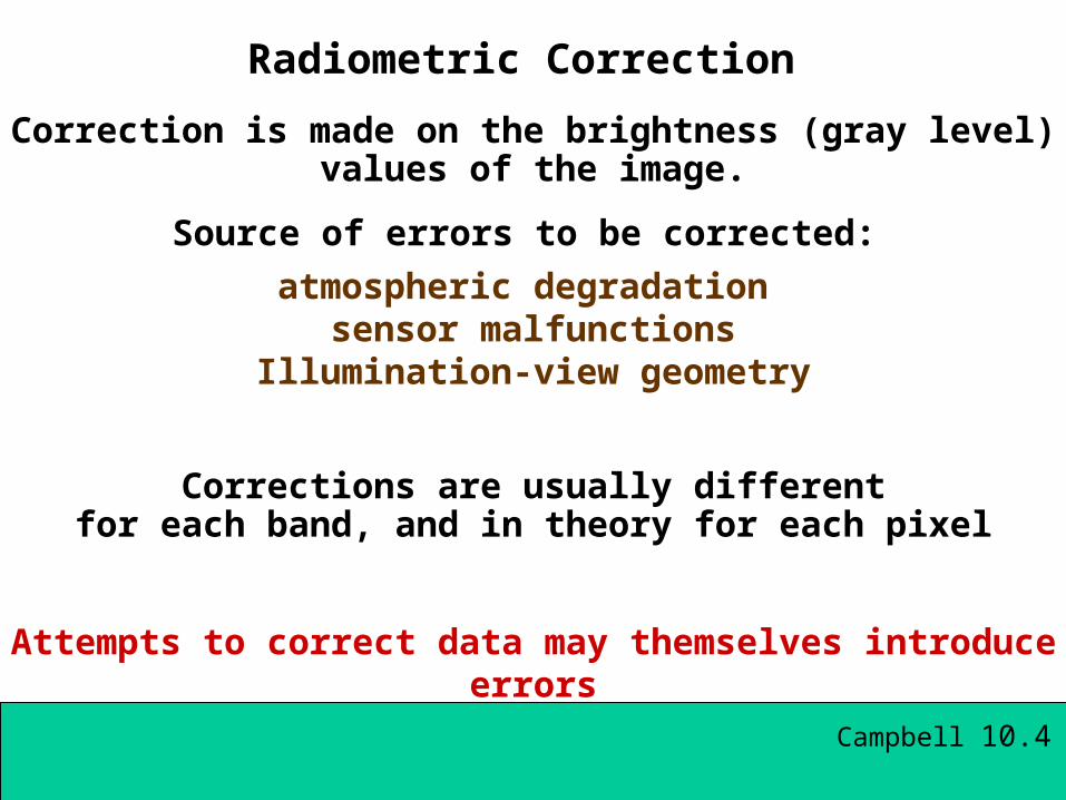
Radiometric Correction

Attempts to correct data may themselves introduce errors

Correction is made on the brightness (gray level) values of the image.

Source of errors to be corrected:

atmospheric degradation sensor malfunctions

Illumination-view geometry

Corrections are usually differentfor each band, and in theory for each pixel

Campbell 10.4

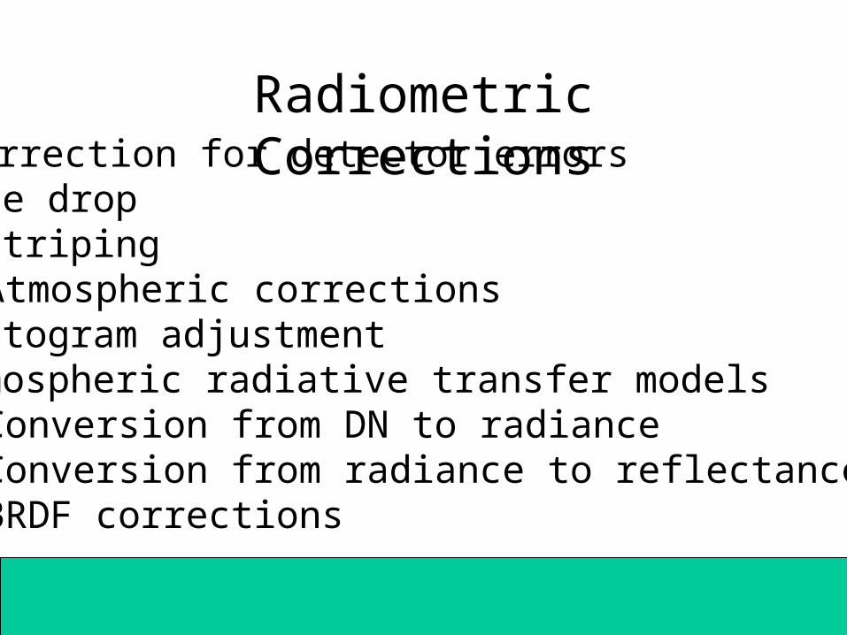
Radiometric Corrections1. Correction for detector errors• Line drop• Destriping2. Atmospheric corrections• Histogram adjustment• Atmospheric radiative transfer models3. Conversion from DN to radiance4. Conversion from radiance to reflectance5. BRDF corrections

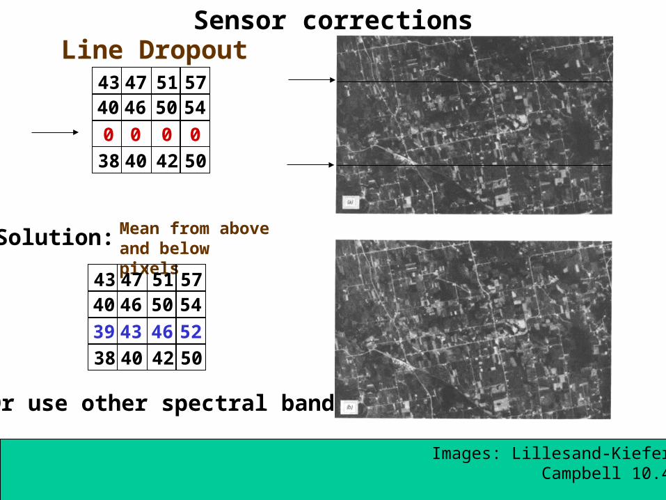
Sensor correctionsLine Dropout

43 47 51 5740 46 50 54

38 40 42 50

0 0 0 0

Solution: Mean from aboveand below pixels

43 47 51 5740 46 50 54

38 40 42 50

39 43 46 52

Or use other spectral band

Images: Lillesand-KieferCampbell 10.4

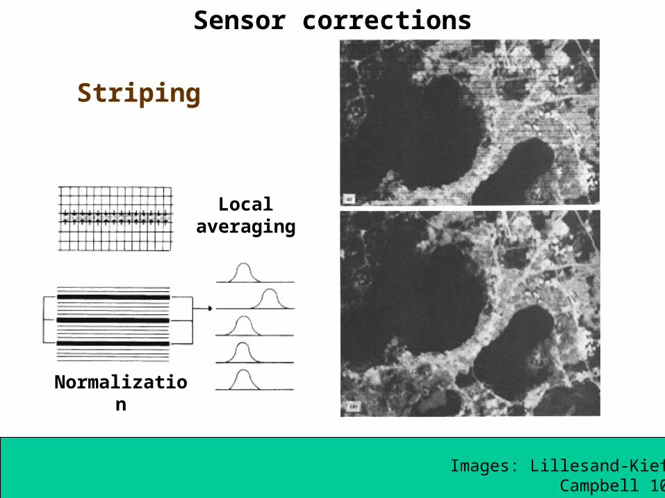
Sensor corrections

Striping

Images: Lillesand-KieferCampbell 10.4

Local averaging

Normalization

Atmospheric Corrections

1) Histogram adjustment• Clear sky• Hazy sky

2) Physical Models

Campbell 10.4

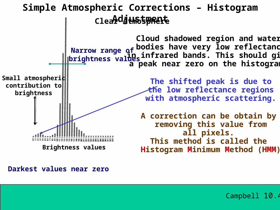
Simple Atmospheric Corrections – Histogram Adjustment

Clear Atmosphere

Small atmosphericcontribution to

brightness

Brightness values

Darkest values near zero

Narrow range of brightness values

Cloud shadowed region and water bodies have very low reflectance

in infrared bands. This should give a peak near zero on the histogram.

The shifted peak is due tothe low reflectance regions

with atmospheric scattering.

A correction can be obtain by removing this value from

all pixels. This method is called the

Histogram Minimum Method (HMM)

Campbell 10.4

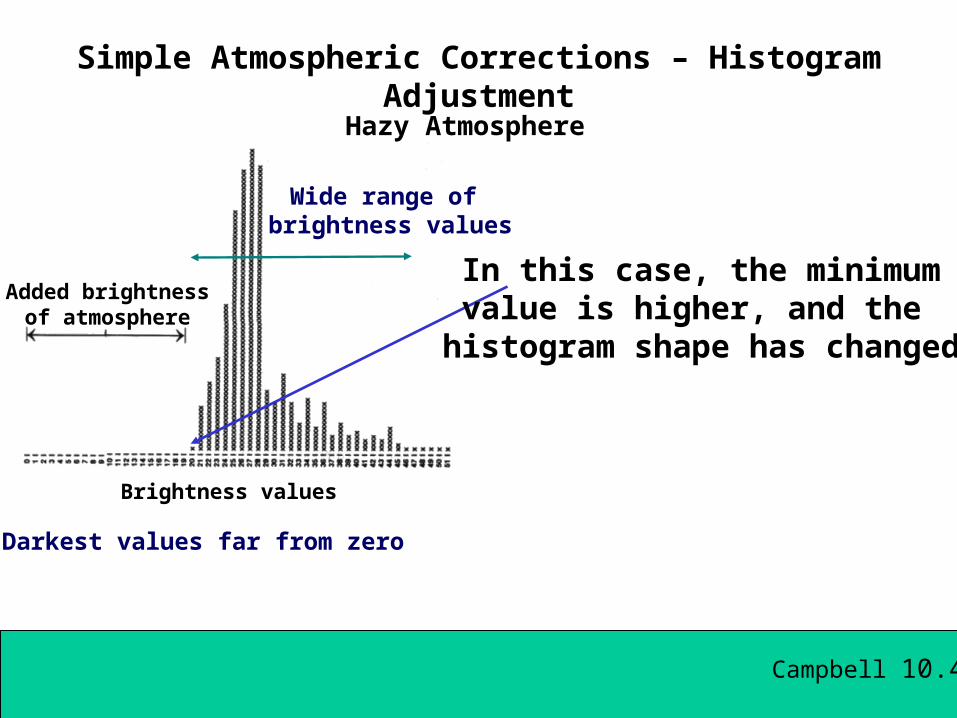
Simple Atmospheric Corrections – Histogram Adjustment

Hazy Atmosphere

Added brightnessof atmosphere

Brightness values

Darkest values far from zero

Wide range of brightness values

In this case, the minimumvalue is higher, and the

histogram shape has changed

Campbell 10.4

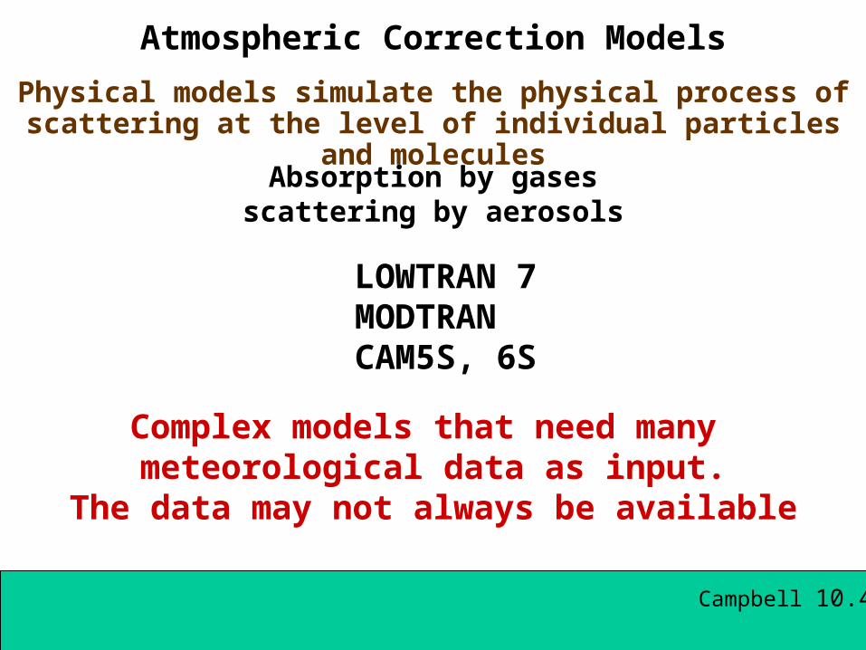
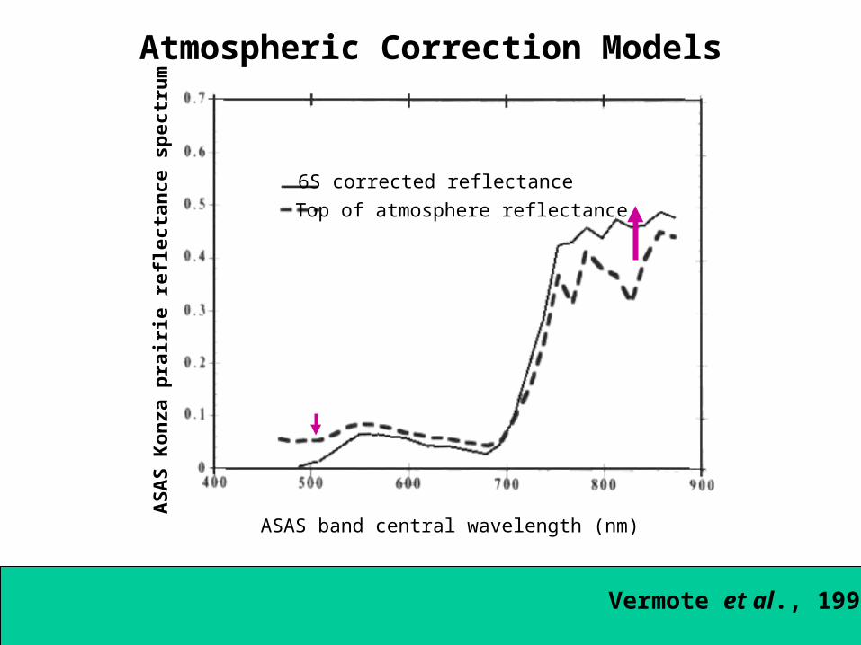
Atmospheric Correction Models

Physical models simulate the physical process of scattering at the level of individual particles and molecules

Complex models that need many meteorological data as input.

The data may not always be available

LOWTRAN 7MODTRANCAM5S, 6S

Absorption by gasesscattering by aerosols

Campbell 10.4

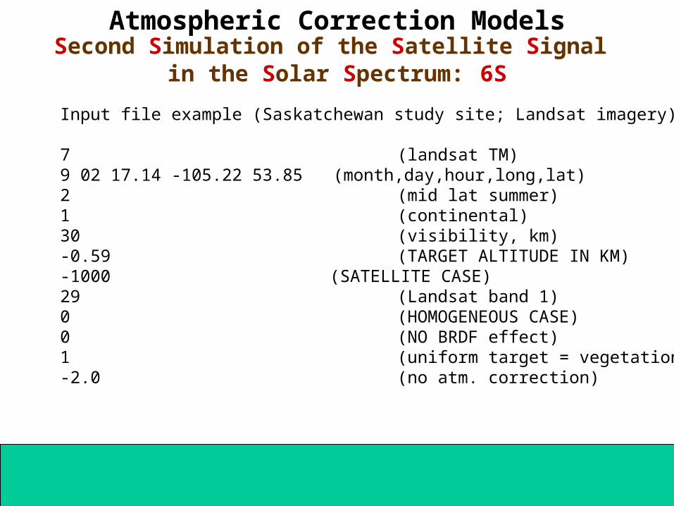
Second Simulation of the Satellite Signal in the Solar Spectrum: 6S

Atmospheric Correction Models

Input file example (Saskatchewan study site; Landsat imagery):

7 (landsat TM)9 02 17.14 -105.22 53.85 (month,day,hour,long,lat)2 (mid lat summer)1 (continental)30 (visibility, km)-0.59 (TARGET ALTITUDE IN KM)-1000 (SATELLITE CASE)29 (Landsat band 1)0 (HOMOGENEOUS CASE)0 (NO BRDF effect)1 (uniform target = vegetation)-2.0 (no atm. correction)

Atmospheric Correction Models

AS

AS

Ko

nza

pra

irie

ref

lect

ance

sp

ectr

um

ASAS band central wavelength (nm)

6S corrected reflectance

Top of atmosphere reflectance

Vermote et al., 1997

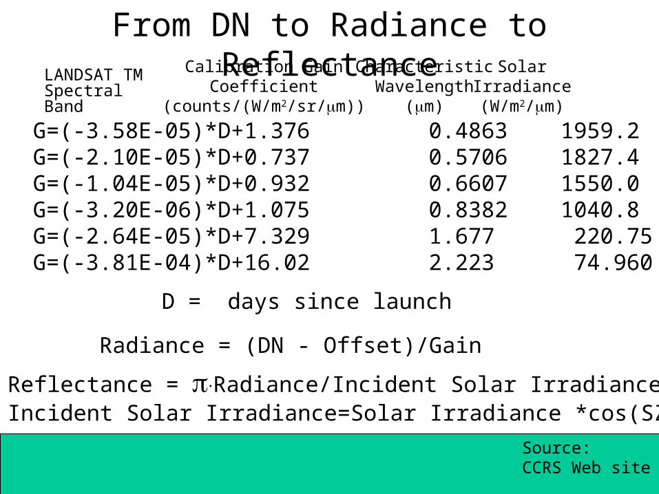
From DN to Radiance to Reflectance

1 G=(-3.58E-05)*D+1.376 0.4863 1959.22 G=(-2.10E-05)*D+0.737 0.5706 1827.43 G=(-1.04E-05)*D+0.932 0.6607 1550.04 G=(-3.20E-06)*D+1.075 0.8382 1040.85 G=(-2.64E-05)*D+7.329 1.677 220.757 G=(-3.81E-04)*D+16.02 2.223 74.960

Source:CCRS Web site

LANDSAT TM Spectral Band

Calibration GainCoefficient

(counts/(W/m2/sr/m))

CharacteristicWavelength

(m)

SolarIrradiance

(W/m2/m)

Radiance = (DN - Offset)/Gain

Reflectance = Radiance/Incident Solar IrradianceIncident Solar Irradiance=Solar Irradiance *cos(SZA)

D = days since launch

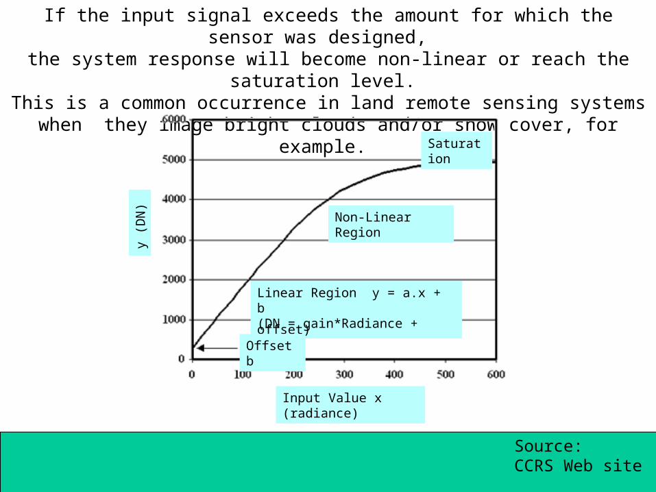
If the input signal exceeds the amount for which the sensor was designed, the system response will become non-linear or reach the saturation level.

This is a common occurrence in land remote sensing systems when they image bright clouds and/or snow cover, for example.

Linear Region y = a.x + b (DN = gain*Radiance + offset)

Non-Linear Region

Saturation

Offset b

Input Value x (radiance)

Source:CCRS Web site

y (D

N)

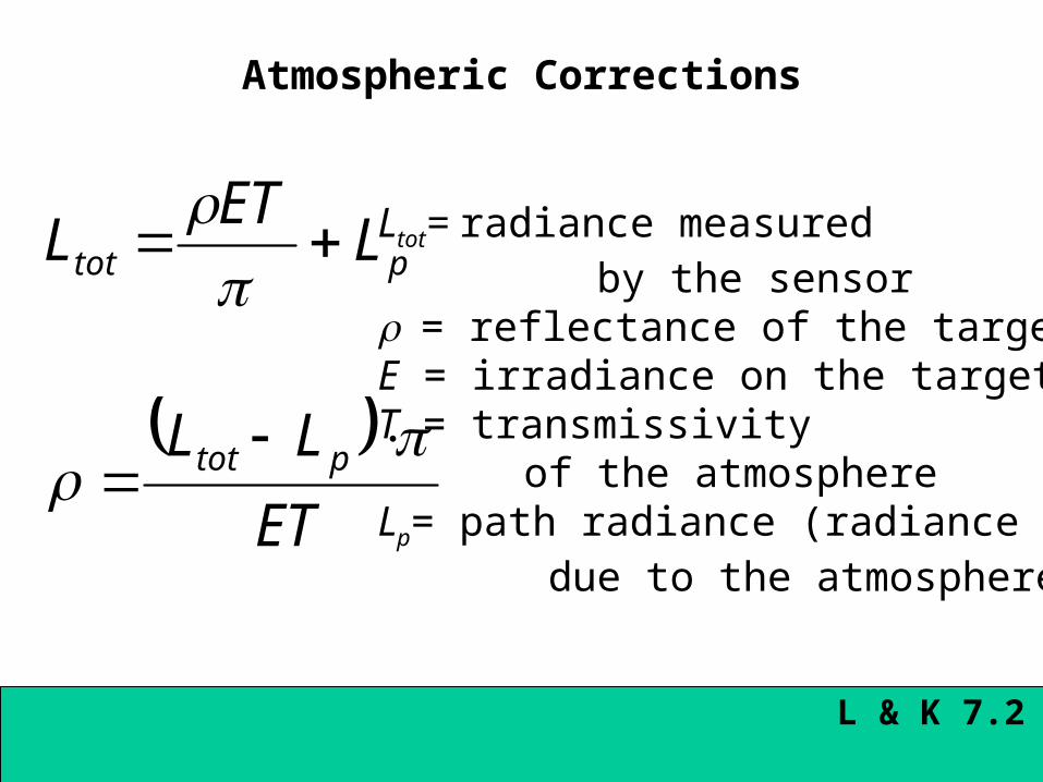
ptot LET

L

ET

LL ptot

Ltot= radiance measured by the sensor= reflectance of the targetE = irradiance on the targetT = transmissivity of the atmosphereLp= path radiance (radiance due to the atmosphere)

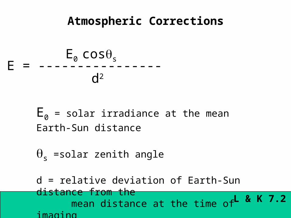
Atmospheric Corrections

L & K 7.2

Atmospheric Corrections

L & K 7.2

E = ----------------E0 coss

d2

E0 = solar irradiance at the mean Earth-Sun distance

s =solar zenith angle

d = relative deviation of Earth-Sun distance from the mean distance at the time of imaging

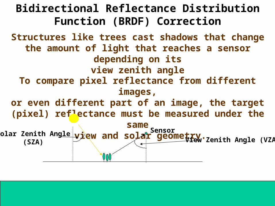
Bidirectional Reflectance Distribution Function (BRDF) Correction

To compare pixel reflectance from different images,or even different part of an image, the target (pixel)

reflectance must be measured under the same view and solar geometry.

Structures like trees cast shadows that change the amount of light that reaches a sensor depending on its

view zenith angle

SensorView Zenith Angle (VZA)

Solar Zenith Angle(SZA)

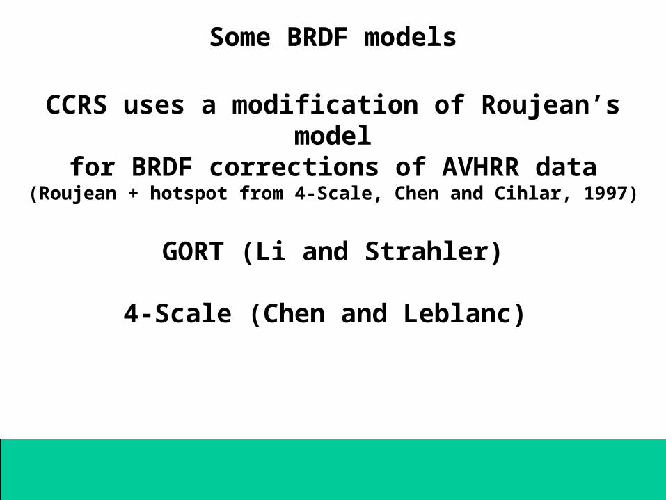
Some BRDF models

CCRS uses a modification of Roujean’s modelfor BRDF corrections of AVHRR data

(Roujean + hotspot from 4-Scale, Chen and Cihlar, 1997)

GORT (Li and Strahler)

4-Scale (Chen and Leblanc)