Embed Size (px)
Citation preview
Power: 1
Hypothesis Testing:
Type II Error and Power

Power: 2
Type I and Type II Error Revisited
Type II error
Type I error
NULL HYPOTHESIS
Actually True Actually False
Fail to
Reject
DECISION
Reject
Either type error is undesirable and we would like both and to be small.
How do we control these?
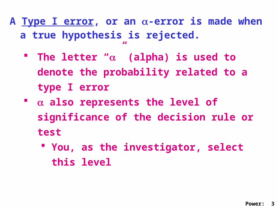
Power: 3
A Type I error, or an -error is made when a true hypothesis is rejected.
The letter “” (alpha) is used to denote the
probability related to a type I error also represents the level of significance of the
decision rule or test You, as the investigator, select this level

Power: 4
A Type II error, or an -error is made when a false hypothesis is NOT rejected.
The letter “” (beta) is used to denote the probability related to a type II error
represents the POWER of a test:
The probability of rejecting a false null hypothesis
The value of depends on a specific alternative hypothesis
can be decreased (power increased) by
increasing sample size

Power: 5
Computing Power of a Test
Example: Suppose we have test of a mean with
Ho: = 100 vs. Ha: 100
= 10
n = 25
= .05
If the true mean is in fact = 105,
what is the probability of failing to reject
Ho when we should ?
What is the power of our test to reject
Ho when we should reject it?
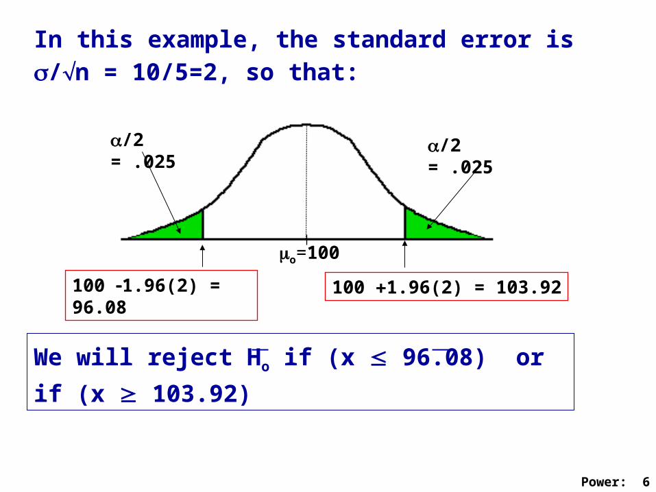
Power: 6
o=100
/2 = .025 /2 = .025
100 1.96(2) = 96.08 100 1.96(2) = 103.92
We will reject Ho if (x 96.08) or if (x 103.92)
In this example, the standard error is /n = 10/5=2, so that:
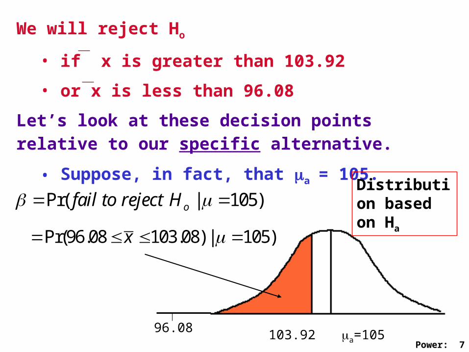
Power: 7
We will reject Ho
• if x is greater than 103.92
• or x is less than 96.08
Let’s look at these decision points relative to our specific alternative.
• Suppose, in fact, that a= 105.
a=105103.9296.08
Distribution based on Ha
Pr( | 105)ofail to reject H
Pr(96.08 103.08) | 105)x
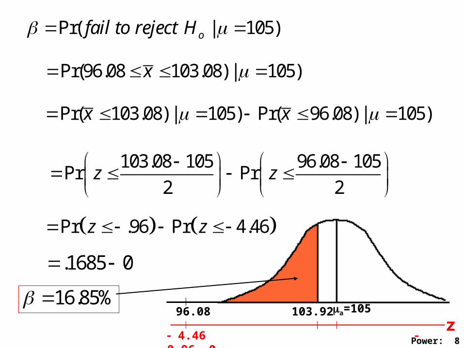
Power: 8
Pr( | 105)ofail to reject H
Pr(96.08 103.08) | 105)x
Pr( 103.08) | 105) Pr( 96.08) | 105)x x
103.08 105 96.08 105Pr Pr
2 2z z
.1685 0
16.85% a=105103.9296.08
Pr .96 Pr 4.46z z
z 4.46 0.96 0

Power: 9
note: is fixed in advance by the investigator depends on
the sample size se = ( / n)
the specific alternative, a
we assume that the variance holds for both
the null and alternative distributions
100-1.96(se) = 96.08 100+1.96(se) = 103.92
/2
0
100
a
105
/2

Power: 10
100-1.96(se) = 96.08 100+1.96(se) = 103.92
/2
0
100
a
105
/2: area where we reject Ho for Ha – Good!
area where we fail to reject Ho even though Ha is correct
Again, looking at our specific alternative: a = 105

Power: 11
We define power as
power = Pr(rejecting Ho | Ha is true)
In our example,
power = = 1 – .1685 = .8315
That is,
• with = .05
• a sample size of n=25
• a true mean of a= 105,
• the power to reject the null hypothesis (o=100)
is 83.15%.
Power: 12
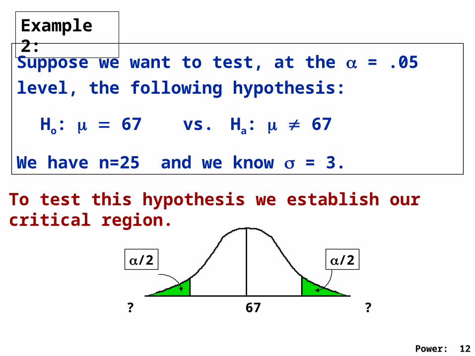
Example 2:
Suppose we want to test, at the = .05 level, the
following hypothesis:
Ho: 67 vs. Ha: 67
We have n=25 and we know = 3.
? 67 ?
/2/2
To test this hypothesis we establish our critical region.

Power: 13
Here, we reject Ho, at the =.05 level when:
or
.975
367 1.96 68.18
5ox zn
.975
367 1.96 65.82
5ox zn
65.82 67 68.18
/2:Rejection region
/2:Rejection region
Power: 14
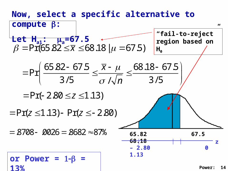
Now, select a specific alternative to compute :
Let Ha1: a=67.5
Pr(65.82 68.18 | 67.5)x
65.82 67.5 68.18 67.5Pr
3/ 5 3/ 5/
x
n
Pr( 2.80 1.13)z
Pr( 1.13) Pr( 2.80)z z
.8708 .0026 .8682 87%
or Power = = 13%
65.82 67.5 68.18
– 2.80 0 1.13z
“fail-to-reject” region based on H0

Power: 15
Now look at the same thing for different values of a:
a zlower zupper Power
68.5 - 4.47 - .53 .29 .71
68 - 3.36 0.30 .62 .38
67.5 - 2.80 1.13 .87 .13
67 - 1.96 1.96 .95 .05
66.5 - 1.13 2.80 .87 .13
66 - 0.30 3.36 .62 .38
65.5 +0.53 4.47 .29 .71
Type II Error () and Power of Test for
= .05, n=25, o = 67, = 3
o
Power: 16
0.00
0.25
0.50
0.75
1.00
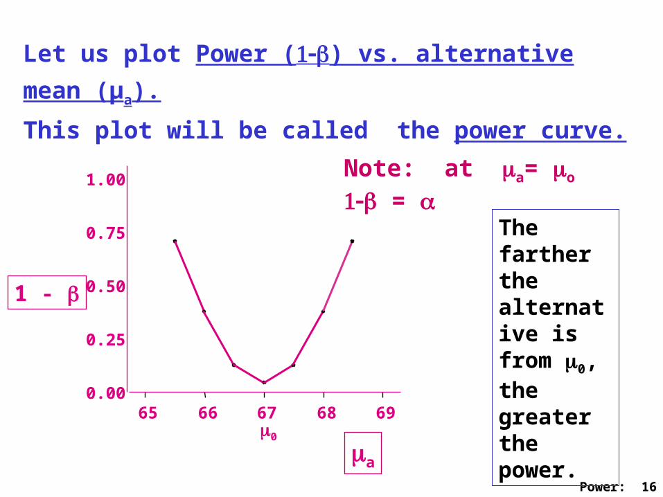
Let us plot Power () vs. alternative mean (µa).
This plot will be called the power curve.
0
65 66 67 68 69
a
1 -
Note: at a= o =
The farther the alternative is from 0, the greater the power.
Power: 17
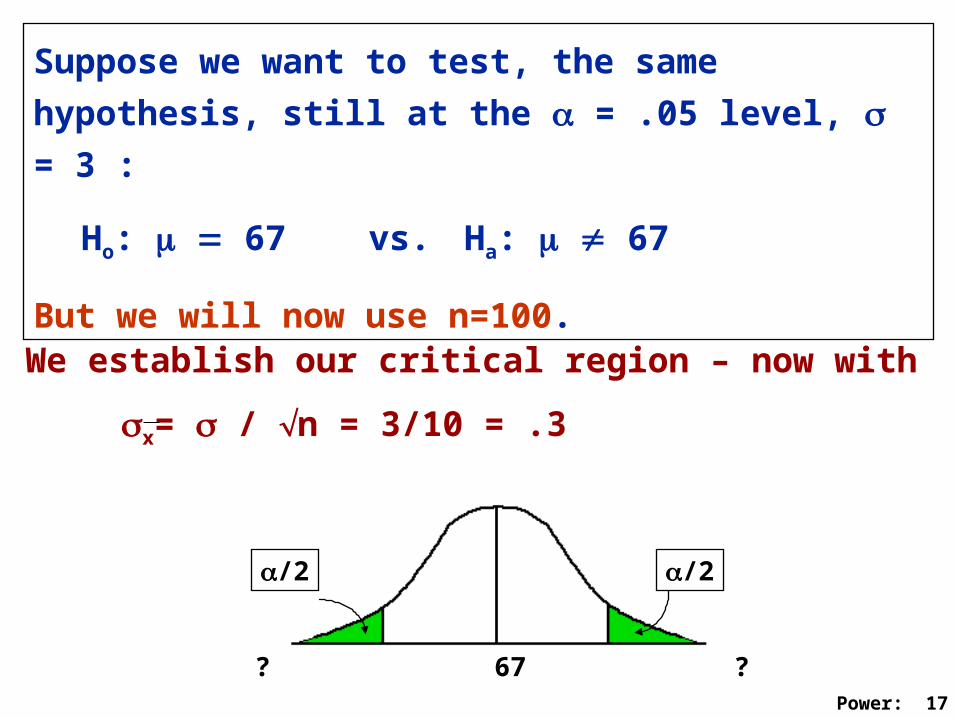
Suppose we want to test, the same hypothesis, still at
the = .05 level, = 3 :
Ho: 67 vs. Ha: 67
But we will now use n=100.
? 67 ?
/2/2
We establish our critical region – now with
x= / n = 3/10 = .3
Power: 18
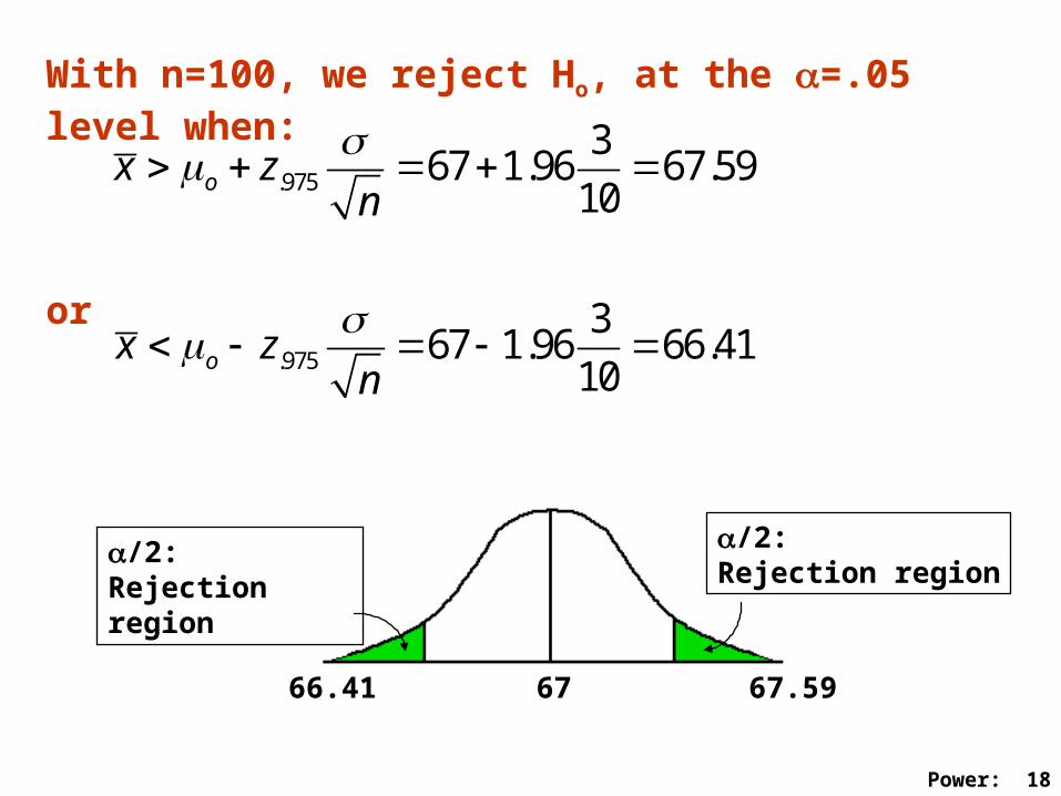
With n=100, we reject Ho, at the =.05 level when:
or
.975
367 1.96 67.59
10ox zn
.975
367 1.96 66.41
10ox zn
66.41 67 67.59
/2:Rejection region
/2:Rejection region

Power: 19
Again, select a specific alternative to compute :
Let Ha: a=67.5
Pr(66.41 67.59 | 67.5)x
66.41 67.5 67.59 67.5Pr
3/10 3/10/
x
n
Pr( 3.63 0.30)z
Pr( 0.30) Pr( 3.36)z z
.6179 .0001 .6178 62%
or Power = = 38%
66.41 67.5 67.59
– 3.63 0 0.30z
“fail-to-reject” region based on H0

Power: 20
a zlower zupper Power
68.5 - 6.97 - 3.04 .00 1.00
68 - 5.30 - 1.37 .09 .91
67.5 - 3.63 0.30 .62 .38
67 - 1.96 1.96 .95 .05
66.5 - 0.30 3.63 .62 .38
66 1.37 5.30 .09 .91
65.5 3.04 6.97 .00 1.00
Type II Error () and Power of Test for
= .05, n=100, o = 67, = 3
o
Now look at the same thing for different values of a:

Power: 21
0.00
0.25
0.50
0.75
1.00
65 66 67 68 69
a
1 -
Power Curves: Power () vs. a for n=25, 100 = .05, o = 67
– n = 100
– n = 25
For the same alternative a, greater n gives greater power.
Power: 22
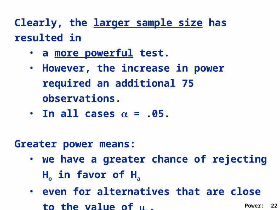
Clearly, the larger sample size has resulted in
• a more powerful test.
• However, the increase in power required an
additional 75 observations.
• In all cases = .05.
Greater power means:
• we have a greater chance of rejecting Ho in
favor of Ha
• even for alternatives that are close to the
value of o.
Power: 23
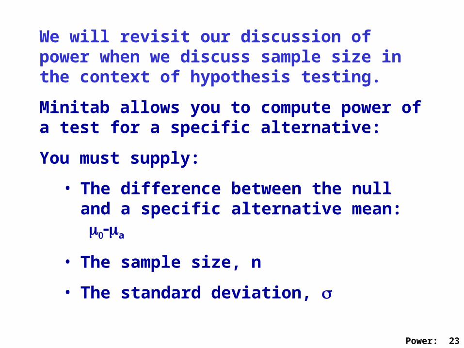
We will revisit our discussion of power when we discuss sample size in the context of hypothesis testing.
Minitab allows you to compute power of a test for a specific alternative:
You must supply:
• The difference between the null and a specific alternative mean: a
• The sample size, n
• The standard deviation,

Power: 24
Using Minitab to estimate Sample Size:
Stat Power and Sample Size 1-Sample Z
Difference between o and a ( to specify several, separate with a space)
Sample size (to specify several, separate with a space)
2-sided test
Power: 25
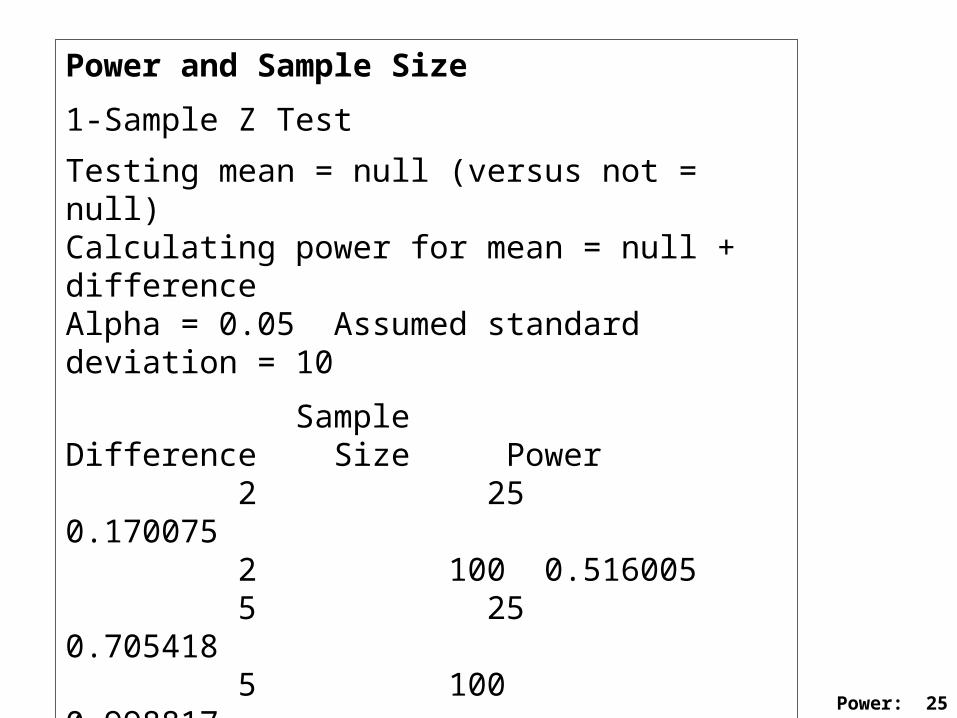
Power and Sample Size
1-Sample Z Test
Testing mean = null (versus not = null)Calculating power for mean = null + differenceAlpha = 0.05 Assumed standard deviation = 10
SampleDifference Size Power 2 25 0.170075 2 100 0.516005 5 25 0.705418 5 100 0.998817


![A-Level Hypothesis and Error - SAT PREP · Test at the 5% significance level the null hypothesis Ho : 1.6 against the alternative hypothesis HI 1.6. [6] A machine is designed to generate](https://img.dokumen.tips/doc/110x75/5ed3eab5b3851038685734b3/a-level-hypothesis-and-error-sat-prep-test-at-the-5-significance-level-the-null.jpg)


![1June 15. 2 In Chapter 17: 17.1 Data [17.2 Risk Difference] [17.3 Hypothesis Test] 17.4 Risk Ratio [17.5 Systematic Sources of Error] [17.6 Power and](https://img.dokumen.tips/doc/110x75/56649d455503460f94a220e6/1june-15-2-in-chapter-17-171-data-172-risk-difference-173-hypothesis.jpg)