The Power of Batching in Multiple Hypothesis Testing

The Power of Batching in Multiple Hypothesis Testing

Tijana Zrnic Daniel L. Jiang Aaditya Ramdas Michael I. JordanUC Berkeley Amazon CMU UC Berkeley

Abstract

One important partition of algorithms forcontrolling the false discovery rate (FDR)in multiple testing is into offline and on-line algorithms. The first generally achievesignificantly higher power of discovery, whilethe latter allow making decisions sequentiallyas well as adaptively formulating hypothe-ses based on past observations. Using exist-ing methodology, it is unclear how one couldtrade off the benefits of these two broad fam-ilies of algorithms, all the while preservingtheir formal FDR guarantees. To this end,we introduce BatchBH and BatchSt-BH, algo-rithms for controlling the FDR when a pos-sibly infinite sequence of batches of hypothe-ses is tested by repeated application of oneof the most widely used offline algorithms,the Benjamini-Hochberg (BH) method orStorey’s improvement of the BH method. Weshow that our algorithms interpolate betweenexisting online and offline methodology, thustrading off the best of both worlds.

1 INTRODUCTION

Consider the setting in which a large number of deci-sions need to be made (e.g., hypotheses to be tested),and one wishes to achieve some form of aggregate con-trol over the quality of these decisions. For binary de-cisions, a seminal line of research has cast this problemin terms of an error metric known as the false discov-ery rate (FDR) (Benjamini and Hochberg, 1995). TheFDR has a Bayesian flavor, conditioning on the deci-sion to reject (i.e., conditioning on a “discovery”) andcomputing the fraction of discoveries that are false.This should be contrasted with traditional metrics—such as sensitivity, specificity, Type I and Type II

Proceedings of the 23rdInternational Conference on Artifi-cial Intelligence and Statistics (AISTATS) 2020, Palermo,Italy. PMLR: Volume 108. Copyright 2020 by the au-thor(s).

errors—where one conditions not on the decision butrather on the hypothesis—whether the null or the al-ternative is true. The scope of research on FDR con-trol has exploded in recent years, with progress onproblems such as dependencies, domain-specific con-straints, and contextual information.

Classical methods for FDR control are “offline” or“batch” methods, taking in a single batch of data andoutputting a set of decisions for all hypotheses at once.This is a serious limitation in the setting of emergingapplications at planetary scale, such as A/B testing inthe IT industry (Kohavi and Longbotham, 2017), andresearchers have responded by developing a range ofonline FDR control methods (Foster and Stine, 2008;Aharoni and Rosset, 2014; Javanmard and Montanari,2018; Ramdas et al., 2018; Tian and Ramdas, 2019).In the online setting, a decision is made at every timestep with no knowledge of future tests, and with pos-sibly infinitely many tests to be conducted overall. Byconstruction, online FDR algorithms guarantee thatthe FDR is controlled during the whole sequence oftests, and not merely at the end.

Online and offline FDR methods both have their prosand cons. Online methods allow the testing of in-finitely many hypotheses, and require less coordina-tion in the setting of multiple decision-makers. Also,perhaps most importantly, they allow the scientist tochoose new hypotheses adaptively, depending on theresults of previous tests. On the other hand, offlineFDR methods tend to make significantly more discov-eries due to the fact that they have access to all teststatistics before making decisions, and not just to theones from past tests. That is, online methods are my-opic, and this can lead to a loss of statistical power.Moreover, the decisions of offline algorithms are sta-ble, in the sense that they are invariant to any im-plicit ordering of hypotheses; this is not true of onlinealgorithms, whose discovery set can vary drasticallydepending on the ordering of hypotheses (Foster andStine, 2008).

By analogy with batch and online methods in gradient-based optimization, these considerations suggest inves-tigating an intermediate notion of “mini-batch,” hop-


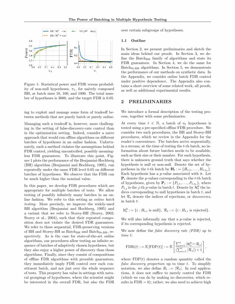
Figure 1: Statistical power and FDR versus probabil-ity of non-null hypotheses, π1, for naively composedBH, at batch sizes 10, 100, and 1000. The total num-ber of hypotheses is 3000, and the target FDR is 0.05.

ing to exploit and manage some form of tradeoff be-tween methods that are purely batch or purely online.

Managing such a tradeoff is, however, more challeng-ing in the setting of false-discovery-rate control thanin the optimization setting. Indeed, consider a naiveapproach that would run offline algorithms on differentbatches of hypotheses in an online fashion. Unfortu-nately, such a method violates the assumptions behindFDR control, yielding uncontrolled, possibly meaning-less FDR guarantees. To illustrate this point, Fig-ure 1 plots the performance of the Benjamini-Hochberg(BH) algorithm (Benjamini and Hochberg, 1995), runrepeatedly under the same FDR level 0.05 on differentbatches of hypotheses. We observe that the FDR canbe much higher than the nominal value.

In this paper, we develop FDR procedures which areappropriate for multiple batches of tests. We allowtesting of possibly infinitely many batches in an on-line fashion. We refer to this setting as online batchtesting. More precisely, we improve the widely-usedBH algorithm (Benjamini and Hochberg, 1995) anda variant that we refer to Storey-BH (Storey, 2002;Storey et al., 2004), such that their repeated compo-sition does not violate the desired FDR guarantees.We refer to these sequential, FDR-preserving versionsof BH and Storey-BH as BatchBH and BatchSt-BH, re-spectively. As is the case for state-of-the-art onlinealgorithms, our procedures allow testing an infinite se-quence of batches of adaptively chosen hypotheses, butthey also enjoy a higher power of discovery than thosealgorithms. Finally, since they consist of compositionsof offline FDR algorithms with provable guarantees,they immediately imply FDR control over each con-stituent batch, and not just over the whole sequenceof tests. This property has value in settings with natu-ral groupings of hypotheses, where the scientist mightbe interested in the overall FDR, but also the FDR

over certain subgroups of hypotheses.

1.1 Outline

In Section 2, we present preliminaries and sketch themain ideas behind our proofs. In Section 3, we de-fine the BatchBH family of algorithms and state itsFDR guarantees. In Section 4, we do the same forBatchSt-BH algorithms. In Section 5, we demonstratethe performance of our methods on synthetic data. Inthe Appendix, we consider online batch FDR controlunder positive dependence. The Appendix also con-tains a short overview of some related work, all proofs,as well as additional experimental results.

2 PRELIMINARIES

We introduce a formal description of the testing pro-cess, together with some preliminaries.

At every time t ∈ N, a batch of nt hypotheses istested using a pre-specified offline FDR procedure. Weconsider two such procedures, the BH and Storey-BHprocedures, which we review in the Appendix for thereader’s convenience. The batches arrive sequentially,in a stream; at the time of testing the t-th batch, no in-formation about future batches needs to be available,such as their size or their number. For each hypothesis,there is unknown ground truth that says whether thehypothesis is null or non-null. Denote the set of hy-potheses in the t-th batch by Ht : = {Ht,1, . . . ,Ht,nt

}.Each hypothesis has a p-value associated with it. LetPt denote the p-values corresponding to the t-th batchof hypotheses, given by Pt : = {Pt,1, . . . , Pt,nt

}, wherePt,j is the j-th p-value in batch t. Denote byH0

t the in-dices corresponding to null hypotheses in batch t, andlet Rt denote the indices of rejections, or discoveries,in batch t:

H0t : = {i : Ht,i is null}, Rt : = {i : Ht,i is rejected}.

We will also informally say that a p-value is rejected,if its corresponding hypothesis is rejected.

We now define the false discovery rate (FDR) up totime t:

FDR(t) : = E [FDP(t)] : = E

[∑ts=1 |H0

s ∩Rs|(∑ts=1 |Rs|) ∨ 1

],

where FDP(t) denotes a random quantity called thefalse discovery proportion up to time t. To simplifynotation, we also define Rt : = |Rt|. In real applica-tions, it does not suffice to merely control the FDR(which we can do by making no discoveries, which re-sults in FDR = 0); rather, we also need to achieve high

Tijana Zrnic, Daniel L. Jiang, Aaditya Ramdas, Michael I. Jordan

statistical power :

Power(t) : = E

[∑ts=1 |([ns] \ H0

s) ∩Rs|∑ts=1 |([ns] \ H0

s)|

],

where [ns] \ H0s are the non-null hypotheses in batch

s.

The goal of the BatchBH procedure is to achieve highpower, while guaranteeing FDR(t) ≤ α for a pre-specified level α ∈ (0, 1) and for all t ∈ N. To doso, the algorithm adaptively determines a test level αtbased on information about past batches of tests, andtests Pt under FDR level αt using the standard BHmethod. The BatchSt-BH method operates in a similarway, the difference being that it uses the Storey-BHmethod for every batch, as opposed to BH.

Define R+t to be the maximum “augmented” number

of rejections in batch t, if one p-value in Pt is “hal-lucinated” to be equal to zero, and all other p-valuesand level αt are held fixed; the maximum is taken overthe choice of the p-value which is set to zero. Moreformally, let At denote a map from a set of p-valuesPt (and implicitly, a level αt) to a set of rejectionsRt. Hence, Rt = |At(Pt)|. In our setting, At will bethe BH algorithm in the case of BatchBH and Storey-BH algorithm in the case of BatchSt-BH. Then, R+

t isdefined as

R+t : = max

i∈[nt]|At(Pt \ Pt,i ∪ 0)|. (1)

Note that R+t could be as large as nt in general. For an

extreme example, let nt = 3, Pt := {2α/3, α, 4α/3},and consider At being the BH procedure. Then Rt =0, while R+

t = 3. However, such “adversarial” p-valuesare unlikely to be encountered in practice and we typi-cally expect R+

t to be roughly equal to Rt+1. In otherwords, we expect that when an unrejected p-value isset to 0, it will be a new rejection, but typically willnot result in other rejections as well. This intuition isconfirmed by our experiments, where we plot R+

t −Rtfor BatchBH with different batch sizes and observe thatthis quantity concentrates around 1. These plots areavailable in Figure 14 in the Appendix.

Let the natural filtration induced by the testing pro-cess be denoted

F t : = σ(P1, . . . ,Pt),

which is the σ-field of all previously observed p-values.Naturally, we require αt to be F t−1-measurable; thetest level at time t is only allowed to depend on infor-mation seen before t. It is worth pointing out that thisfiltration is different from the corresponding filtrationin prior online FDR work, which was typically of the

form σ(R1, . . . , Rt). The benefits of this latter, smallerfiltration arise when proving modified FDR (mFDR)guarantees, which we do not consider in this paper.Moreover, a richer filtration allows more freedom inchoosing αt, making our choice of F t a natural one.

For the formal guarantees of BatchBH and BatchSt-BH,we will require the procedures to be mono-tone. Let ({P1,1, . . . , P1,n1

}, . . . , {Pt,1, . . . , Pt,nt})

and ({P̃1,1, . . . , P̃1,n1}, . . . , {P̃t,1, . . . , P̃t,nt}) be two se-quences of p-value batches, which are identical in allentries but (s, i), for some s ≤ t: P̃s,i < Ps,i. Then,

a procedure is monotone if

t∑r=s+1

Rr ≤t∑

r=s+1

R̃r.

Intuitively, this condition says that making any of thetested p-values smaller can only make the overall num-ber of rejections larger. A similar assumption appearsin online FDR literature (Javanmard and Montanari,2018; Ramdas et al., 2018; Zrnic et al., 2018; Tian andRamdas, 2019). In general, whether or not a proce-dure is monotone is a property of the p-value distri-bution; notice, however, that monotonicity can be as-sessed empirically (it does not depend on the unknownground truth). One way to ensure monotonicity is tomake αt a coordinate-wise non-increasing function of(P1,1, . . . , P1,n1 , P2,1, . . . , Pt−1,nt−1). In the Appendix,we give examples of monotone strategies.

Finally, we review a basic property of null p-values. Ifa hypothesis Ht,i is truly null, then the correspondingp-value Pt,i stochastically dominates the uniform dis-tribution, or is super-uniformly distributed, meaning:

If Ht,i is null, then P{Pt,i ≤ u} ≤ u for all u ∈ [0, 1].

2.1 Algorithms via Empirical FDP Estimates

We build on Storey’s interpretation of the BH proce-dure (Storey, 2002) as an empirical Bayesian proce-dure, based on empirical estimates of the false discov-ery proportion. In this section, we give a sketch ofthis idea, as it is at the core of our algorithmic con-structions. The steps presented below are not fullyrigorous, but are simply meant to develop intuition.

When an algorithm decides to reject a hypothesis,there is generally no way of knowing if the rejectedhypothesis is null or non-null. Consequently, it is im-possible for the scientist to know the achieved FDP.However, by exploiting the super-uniformity of null p-values, it is possible to estimate the behavior of theFDP on average. More explicitly, there are tools thatutilize only the information available to the scientistto upper bound the average FDP, that is the FDR.

We sketch this argument for the BatchBH procedure


here, formalizing the argument in Theorem 1. The-orem 2 gives an analogous proof for the BatchSt-BH

procedure.

By definition, the FDR is equal to

E

[∑ts=1 |H

0s ∩Rs|

(∑tr=1 |Rr|) ∨ 1

]=

t∑s=1

E

∑i∈H0

s1{Ps,i ≤ αs

nsRs

}(∑tr=1 |Rr|) ∨ 1

,

where we use the definition of the BH procedure. Ifthe p-values are independent, we will show that it isvalid to upper bound this expression by inserting anexpectation in the numerator, approximately as

t∑s=1

E

∑i∈H0sP{Ps,i ≤ αs

nsRs

∣∣∣ αs, Rs}(∑tr=1 |Rr|) ∨ 1

.Invoking the super-uniformity of null p-values (andtemporarily ignoring dependence between Ps,i andRs), we get

t∑s=1

E

[|H0

s|αs

nsRs

(∑tr=1 |Rr|) ∨ 1

]≤ E

[ ∑ts=1 αsRs

(∑tr=1 |Rr|) ∨ 1

].

Suppose we define F̂DPBatchBH(t) ≈

∑ts=1 αsRs

(∑t

r=1 |Rr|)∨1.

This quantity is purely empirical ; each term is knownto the scientist. Hence, by an appropriate choice of αsat each step, one can ensure that F̂DPBatchBH(t) ≤ αfor all t. But by the sketch given above, this wouldimmediately imply FDR ≤ α, as desired. This proofsketch is the core idea behind our algorithms.

It is important to point out that there is not a single

way of ensuring F̂DPBatchBH(t) ≤ α; this approach

gives rise to a whole family of algorithms. Naturally,the choice of αs can be guided by prior knowledge orimportance of a given batch, as long as the empiricalestimate is controlled under α.

3 ONLINE BATCH FDR CONTROLVIA BatchBH

In this section, we define the BatchBH class of algo-rithms and state our main technical result regardingits FDR guarantees.

Definition 1 (BatchBH). The BatchBH procedure isany rule for assigning test levels αs such that

F̂DPBatchBH(t) : =

∑s≤t

αsR+s

R+s +

∑r≤t,r 6=sRr

is always controlled under a pre-determined level α.

Note that if we were to approximate R+s by Rs, we

would arrive exactly at the estimate derived in theproof sketch of the previous section.

This way of controlling F̂DPBatchBH(t) interpolates be-tween prior offline and online FDR approaches. First,suppose that there is only one batch. Then, the useris free to pick α1 to be any level less than or equal toα, in which case it makes sense to simply pick α. Onthe other hand, if every batch is of size one we haveR+s = 1, hence the FDP estimate reduces to

F̂DPBatchBH(t) =

∑s≤t

αs1 +

∑r≤t,r 6=sRr

≤∑s≤t αs∑r≤tRr

: = F̂DPLORD(t),

where the intermediate inequality is almost an equal-ity whenever the total number of rejections is non-

negligible. The quantity F̂DPLORD(t) is an estimateof FDP that is implicitly used in an existing online al-gorithm known as LORD (Javanmard and Montanari,2018), as detailed by Ramdas et al. (2017). Thus,BatchBH can be seen as a generalization of both BHand LORD, simultaneously allowing arbitrary batchsizes (like BH) and an arbitrary number of batches(like LORD).

We now state our main formal result regarding FDRcontrol of BatchBH. As suggested in Section 2, to-

gether with the requirement that F̂DPBatchBH(t) ≤ α

for all t ∈ N we also need to guarantee that the pro-cedure is monotone. Recall that monotonicity roughlymeans that making any of the tested p-values smallercan only result in more rejections. In general, anyreasonable update for αt satisfying Definition 1 is ex-pected to be monotone for non-adversarially chosenp-values. We analyze one such natural update in Sec-tion 5. However, one can also construct more conserva-tive algorithms which are guaranteed to be monotoneuniformly across all p-value sequences. We presentmultiple such procedures in the Appendix.

Theorem 1. If all null p-values in the sequence areindependent of each other and the non-nulls, and theBatchBH procedure is monotone, then it provides any-time FDR control: for every t ∈ N, FDR(t) ≤ α.

We defer the proof of Theorem 1 to the Appendix.

4 ONLINE BATCH FDR CONTROLVIA BatchSt-BH

In addition to the FDR level α, the Storey-BH algo-rithm also requires a user-chosen constant λ ∈ (0, 1)as a parameter. This extra parameter allows the algo-rithm to be more adaptive to the data at hand, con-structing a better FDP estimate (Storey, 2002). Werevisit this estimate in the Appendix.


Thus, our extension of Storey-BH, BatchSt-BH, re-quires a user-chosen constant λt ∈ (0, 1) as an inputto the algorithm at time t ∈ N. Unless there is priorknowledge of the p-value distribution, it is a reason-able heuristic to simply set λt = 0.5 for all t (Storey,2002; Storey et al., 2004).

Denote by maxt : = arg maxi{Pt,i : i ∈ [nt]} the in-dex corresponding to the maximum p-value in batcht. With this, define the null proportion sensitivity forbatch t as:

kt : =

∑i≤nt

1 {Pt,i > λt}1 +

∑j≤nt,j 6=maxt

1 {Pt,j > λt}.

Now we can define the BatchSt-BH family of methods.

Definition 2. The BatchSt-BH procedure is any rulefor assigning test levels αs, such that

F̂DPBatchSt-BH(t) : =∑s≤t

αsksR+s

R+s +

∑r≤t,r 6=sRr

is controlled under a pre-determined level α.

Just like BatchBH, BatchSt-BH likewise interpolates be-tween existing offline and online FDR procedures. Ifthere is a single batch of tests, the user can pick thetest level α1 to be at most α, in which case it makessense to simply pick α. This follows due to ki ≤ 1 bydefinition. On the other end of the spectrum, in thefully online setting, BatchSt-BH reduces to the SAF-FRON procedure (Ramdas et al., 2018). Indeed, sincekt = 1 {Pt,1 > λt}, the FDP estimate reduces to:

F̂DPBatchSt-BH(t) =

∑s≤t

αs1 {Ps,1 > λs}1 +

∑r≤t,r 6=sRr

≤∑s≤t αs1 {Ps,1 > λs}∑

r≤tRr

: = F̂DPSAFFRON(t),

which is equivalent to the FDP estimate defined byRamdas et al. (2018). We discuss the connections be-tween the two FDP estimates in more detail in theAppendix.

We are now ready to state our main result forBatchSt-BH. Just like BatchBH, the BatchSt-BH pro-cedure requires monotonicity to control the FDR (asper the argument outlined in Section 2). We describemultiple monotone versions of BatchSt-BH in the Ap-pendix, and discuss some useful heuristics in Section 5.

Theorem 2. If the null p-values in the sequence areindependent of each other and the non-nulls, and theBatchSt-BH procedure is monotone, then it providesanytime FDR control: for every t ∈ N, FDR(t) ≤ α.

The proof of Theorem 2 is presented in the Appendix.

5 NUMERICAL EXPERIMENTS

We compare the performance of BatchBH andBatchSt-BH with two state-of-the-art online FDR al-gorithms: LORD (Javanmard and Montanari, 2018;Ramdas et al., 2017) and SAFFRON (Ramdas et al.,2018). Specifically, we compare the achieved powerand FDR of these methods on synthetic data, while inthe Appendix we study a real fraud detection data set.

As explained in prior literature (Ramdas et al., 2018),LORD and BH are non-adaptive methods, while SAF-FRON and Storey-BH adapt to the tested p-valuesthrough the parameter λt. We keep comparisons fairby comparing BatchBH with LORD, and BatchSt-BH

with SAFFRON.

As discussed in Section 2, there are various ways toassign αi such that the appropriate FDP estimate iscontrolled under α. Moreover, as we argued in Sec-tion 3 and Section 4, this needs to be done in a mono-tone way to guarantee FDR control for an arbitraryp-value distribution. In the experimental sections ofthis paper, however, we resort to a heuristic. Enforc-ing monotonicity uniformly across all distributions di-minishes the power of FDR methods. Hence, we applyalgorithms which control the corresponding FDP esti-mates and are expected to be monotone under naturalp-value distributions, but possibly not for adversariallychosen ones. In the Appendix we test the monotonic-ity of these procedures empirically, and demonstratethat it is satisfied with overwhelming probability. Wenow present the specific algorithms that we studied.

Algorithm 1 The BatchBH algorithm

Input: FDR level α, non-negative sequence {γs}∞s=1

such that∑∞s=1 γs = 1.

Set α1 = γ1α;for t = 1, 2, . . . do

Run the BH method at level αt on batch Pt;

Set βt+1 =∑s≤t αs

R+s

R+s +

∑r 6=s,r≤t Rr

;

Set αt+1 =(∑

s≤t+1 γsα− βt+1

)nt+1+

∑s≤t Rs

nt+1;

end

Algorithm 2 The BatchSt-BH algorithm

Input: FDR level α, non-negative sequence {γs}∞s=1

such that∑∞s=1 γs = 1

Set α1 = γ1α;for t = 1, 2, . . . do

Run the Storey-BH method at level αt with pa-rameter λt on batch Pt;

Set βt+1 =∑s≤t ksαs

R+s

R+s +

∑r 6=s,r≤t Rr

;

Set αt+1 =(∑

s≤t+1 γsα− βt+1

)nt+1+

∑s≤t Rs

nt+1;

end


The choice of λt should generally depend on the num-ber and strength of non-null p-values the analyst ex-pects to see in the sequence. As suggested in previ-ous works on similar adaptive methods (Storey, 2002;Storey et al., 2004; Ramdas et al., 2018), it is reason-able to set λt ≡ 0.5 if no prior knowledge is assumed.

The reason why we add a sequence {γs}∞s=1 as a hy-perparameter is to prevent αt from vanishing. If weimmediately invest the whole error budget α, i.e. weset γ1 = 1 and γs = 0, s 6= 1, then αt might be closeto 0 for small batches, given that R+

t could be closeto nt. For this reason, for the smallest batch size weconsider (which is 10), we pick γs ∝ s−2. Similar errorbudget investment strategies have been considered inprior work (Ramdas et al., 2018; Tian and Ramdas,2019). For larger batch sizes, R+

t is generally muchsmaller than nt, so for all other batch sizes we investmore aggressively by picking γ1 = γ2 = 1

2 , γs = 0,s 6∈ {1, 2}. This is analogous to the default choiceof “initial wealth” for LORD and SAFFRON of α

2 ,which we also use in our experiments. We only adaptour choice of {γs}∞s=1 to the batch size, as that is in-formation available to the scientist. In general, onecan achieve better power if {γs}∞s=1 is tailored to pa-rameters such as the number of non-nulls and theirstrength, but given that such information is typicallyunknown, we keep our hyperparameters agnostic tosuch specifics.

In the Appendix we prove Fact 1, which states theAlgorithm 1 controls the appropriate FDP estimate.We omit the analogous proof for Algorithm 2 due tothe similarity of the two proofs.

Fact 1. Algorithm 1 maintains F̂DPBatchBH(t) ≤ α.

We test for the means of a sequence of T = 3000 in-dependent Gaussian observations. Under the null, themean is µ0 = 0. Under the alternative, the mean is µ1,whose distribution differs in two settings that we stud-ied. For each index i ∈ {1, . . . , T}, the observation Ziis distributed according to

Zi ∼

{N(µ0, 1),with probability 1− π1,N(µ1, 1),with probability π1.

In all experiments we set α = 0.05. All plotsdisplay the average and one standard deviationaround the average of power or FDR, against π1 ∈{0.01, 0.02, . . . , 0.09} ∪ {0.1, 0.2, 0.3, 0.4, 0.5} (interpo-lated for in-between values). All quantities are aver-aged over 500 independent trials.

5.1 Constant Gaussian Means

In this setting, we choose the mean under the alterna-tive to be constant, µ1 = 3. Each observation is con-

Figure 2: Statistical power and FDR versus probabil-ity of non-null hypotheses π1 for BatchBH (at batchsizes 10, 100, and 1000) and LORD. The observationsunder the null are N(0, 1), and the observations underthe alternative are N(3, 1).

Figure 3: Statistical power and FDR versus probabil-ity of non-null hypotheses π1 for BatchSt-BH (at batchsizes 10, 100, and 1000) and SAFFRON. The observa-tions under the null are N(0, 1), and the observationsunder the alternative are N(3, 1).

verted to a one-sided p-value as Pi = Φ(−Zi), whereΦ is the standard Gaussian CDF.

Non-adaptive procedures. Figure 2 compares thestatistical power and FDR of BatchBH and LORD asfunctions of π1. Across almost all values of π1, the on-line batch procedures outperform LORD, with the ex-ception of BatchBH with the smallest considered batchsize, for small values of π1.

Adaptive procedures. Figure 3 compares the sta-tistical power and FDR of BatchSt-BH and SAFFRONas functions of π1. The online batch procedures domi-nate SAFFRON for all values of π1. The difference inpower is especially significant for π1 ≤ 0.1, which is areasonable range for the non-null proportion in mostreal-world applications.


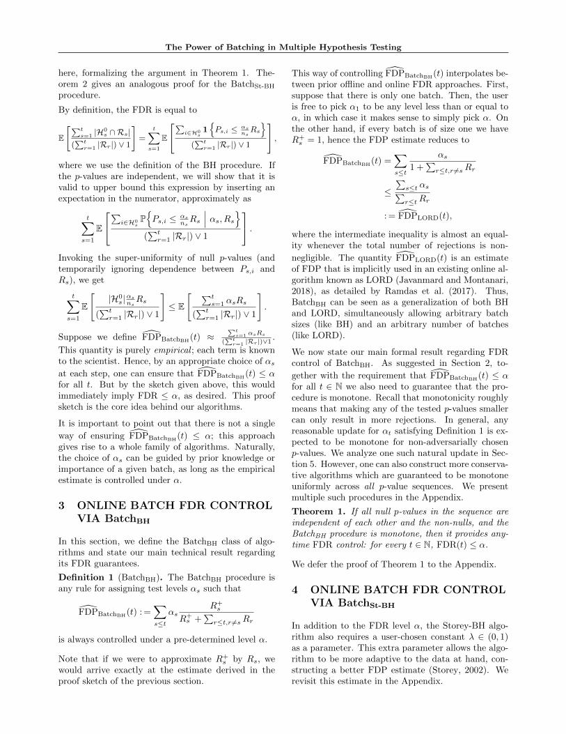
Figure 4: Statistical power and FDR versus probabil-ity of non-null hypotheses π1 for naively composed BH(at batch sizes 10, 100, and 1000). The observationsunder the null are N(0, 1), and the observations underthe alternative are N(3, 1).

Figure 5: Statistical power and FDR versus proba-bility of non-null hypotheses π1 for naively composedStorey-BH (at batch sizes 10, 100, and 1000). Theobservations under the null are N(0, 1), and the ob-servations under the alternative are N(3, 1).

Naively composed procedures. Figure 4 and Fig-ure 5 show the statistical power and FDR versus π1for BH and Storey-BH naively run in a batch settingwhere each individual batch is run using test levelα = 0.05. Although there is a significant boost inpower, the FDR is generally much higher than the de-sired value for reasonably small π1; this is not true ofbatch size 1000 because only 3 batches are composed,where we know that in the worst case FDR ≤ 3α.

5.2 Random Gaussian Alternative Means

Now we consider random alternative means; we letµ1 ∼ N(0, 2 log T ). Unlike the previous setting, this isa hard testing problem in which non-nulls are barelydetectable (Javanmard and Montanari, 2018). Eachobservation is converted to a two-sided p-value as Pi =2Φ(−|Zi|), where Φ is the standard Gaussian CDF.

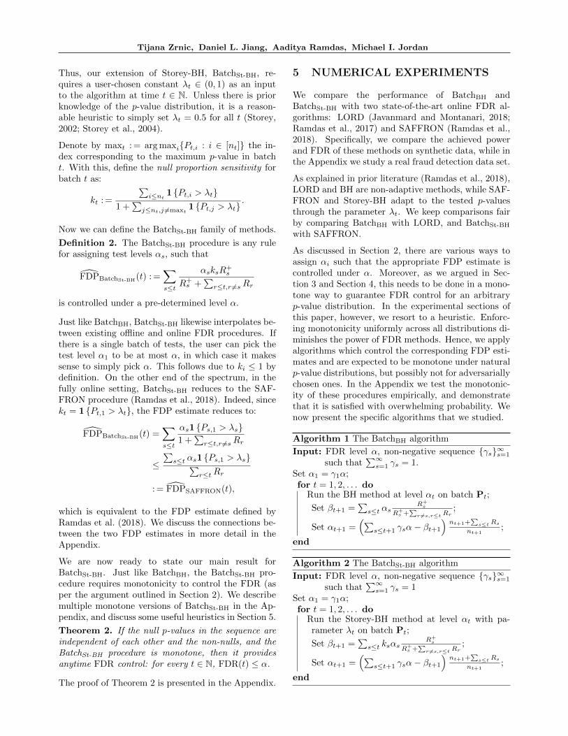
Figure 6: Statistical power and FDR versus probabil-ity of non-null hypotheses π1 for BatchBH (at batchsizes 10, 100, and 1000) and LORD. The observationsunder the null are N(0, 1), and the observations underthe alternative are N(µ1, 1) where µ1 ∼ N(0, 2 log T ).

Figure 7: Statistical power and FDR versus proba-bility of non-null hypotheses π1 for BatchSt-BH (atbatch sizes 10, 100, and 1000) and SAFFRON. Theobservations under the null are N(0, 1), and the ob-servations under the alternative are N(µ1, 1) whereµ1 ∼ N(0, 2 log T ).

Non-adaptive procedures. Figure 6 compares thestatistical power and FDR of BatchBH and LORD asfunctions of π1. Again, for most values of π1 all batchprocedures outperform LORD.

Adaptive procedures. Figure 7 compares the sta-tistical power and FDR of BatchSt-BH and SAFFRONas functions of π1. For high values of π1, all proceduresbehave similarly, while for small values of π1 the batchprocedures dominate.

Naively composed procedures. Figure 8 and Fig-ure 9 show the statistical power and FDR versus π1for BH and Storey-BH naively run in a batch set-ting where each individual batch is run using test levelα = 0.05. In this hard testing problem, there is not asmuch gain in power, and the FDR is extremely high,as expected.


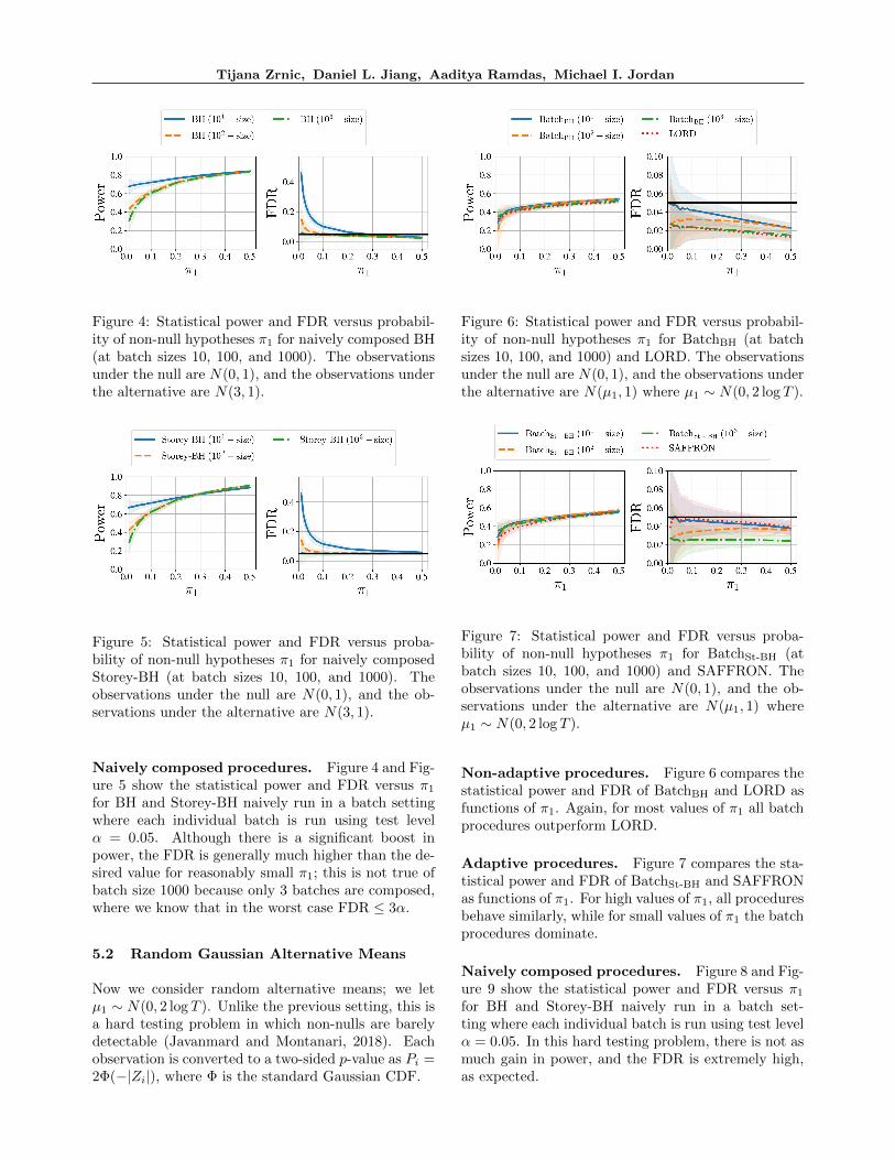
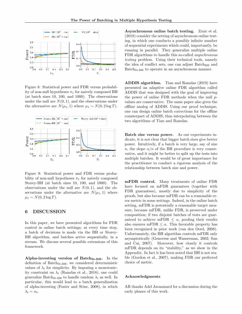
Figure 8: Statistical power and FDR versus probabil-ity of non-null hypotheses π1 for naively composed BH(at batch sizes 10, 100, and 1000). The observationsunder the null are N(0, 1), and the observations underthe alternative are N(µ1, 1) where µ1 ∼ N(0, 2 log T ).

Figure 9: Statistical power and FDR versus proba-bility of non-null hypotheses π1 for naively composedStorey-BH (at batch sizes 10, 100, and 1000). Theobservations under the null are N(0, 1), and the ob-servations under the alternative are N(µ1, 1) whereµ1 ∼ N(0, 2 log T ).

6 DISCUSSION

In this paper, we have presented algorithms for FDRcontrol in online batch settings; at every time step,a batch of decisions is made via the BH or Storey-BH algorithm, and batches arrive sequentially, in astream. We discuss several possible extensions of thisframework.

Alpha-investing version of BatchSt-BH. In thedefinition of BatchSt-BH, we considered deterministicvalues of λt for simplicity. By imposing a monotonic-ity constraint on λt (Ramdas et al., 2018), one couldgeneralize BatchSt-BH to handle random λt as well. Inparticular, this would lead to a batch generalizationof alpha-investing (Foster and Stine, 2008), in whichλt = αt.

Asynchronous online batch testing. Zrnic et al.(2018) consider the setting of asynchronous online test-ing, in which one conducts a possibly infinite numberof sequential experiments which could, importantly, berunning in parallel. They generalize multiple onlineFDR algorithms to handle this so-called asynchronoustesting problem. Using their technical tools, namelythe idea of conflict sets, one can adjust BatchBH andBatchSt-BH to operate in an asynchronous manner.

ADDIS algorithm. Tian and Ramdas (2019) havepresented an adaptive online FDR algorithm calledADDIS that was designed with the goal of improvingthe power of online FDR methods when the null p-values are conservative. The same paper also gives theoffline analog of ADDIS. Using our proof technique,one can design online batch corrections for the offlinecounterpart of ADDIS, thus interpolating between thetwo algorithms of Tian and Ramdas.

Batch size versus power. As our experiments in-dicate, it is not clear that bigger batch sizes give betterpower. Intuitively, if a batch is very large, say of sizen, the slope α/n of the BH procedure is very conser-vative, and it might be better to split up the tests intomultiple batches. It would be of great importance forthe practitioner to conduct a rigorous analysis of therelationship between batch size and power.

mFDR control. Many treatments of online FDRhave focused on mFDR guarantees (together withFDR guarantees), mostly due to simplicity of theproofs, but also because mFDR can be a reasonable er-ror metric in some settings. Indeed, in the online batchsetting, mFDR is potentially a reasonable target mea-sure, because mFDR, unlike FDR, is preserved undercomposition; if two disjoint batches of tests are guar-anteed to achieve mFDR ≤ α, pooling their resultsalso ensures mFDR ≤ α. This favorable property hasbeen recognized in prior work (van den Oord, 2008).Unfortunately, the BH algorithm controls mFDR onlyasymptotically (Genovese and Wasserman, 2002; Sunand Cai, 2007). Moreover, how closely it controlsmFDR depends on its “stability,” as we show in theAppendix. In fact it has been noted that BH is not sta-ble (Gordon et al., 2007), making FDR our preferredchoice of metric.

Acknowledgments

AR thanks Adel Javanmard for a discussion during theearly phases of this work.


References

Ehud Aharoni and Saharon Rosset. Generalized α-investing: definitions, optimality results and appli-cation to public databases. Journal of the RoyalStatistical Society, Series B (Statistical Methodol-ogy), 76(4):771–794, 2014.

Yoav Benjamini and Yosef Hochberg. Controlling thefalse discovery rate: a practical and powerful ap-proach to multiple testing. Journal of the RoyalStatistical Society, Series B (Methodological), 57(1):289–300, 1995.

Dean Foster and Robert Stine. α-investing: a proce-dure for sequential control of expected false discov-eries. Journal of the Royal Statistical Society, SeriesB (Statistical Methodology), 70(2):429–444, 2008.

Christopher Genovese and Larry Wasserman. Operat-ing characteristics and extensions of the false discov-ery rate procedure. Journal of the Royal StatisticalSociety: Series B (Statistical Methodology), 64(3):499–517, 2002.

Alexander Gordon, Galina Glazko, Xing Qiu, AndreiYakovlev, et al. Control of the mean number offalse discoveries, bonferroni and stability of multipletesting. The Annals of Applied Statistics, 1(1):179–190, 2007.

Adel Javanmard and Andrea Montanari. Online rulesfor control of false discovery rate and false discoveryexceedance. The Annals of Statistics, 46(2):526–554,2018.

Ron Kohavi and Roger Longbotham. Online con-trolled experiments and a/b testing. Encyclopediaof machine learning and data mining, pages 922–929, 2017.

Aaditya Ramdas, Fanny Yang, Martin Wainwright,and Michael Jordan. Online control of the false dis-covery rate with decaying memory. In AdvancesIn Neural Information Processing Systems, pages5655–5664, 2017.

Aaditya Ramdas, Tijana Zrnic, Martin Wainwright,and Michael Jordan. SAFFRON: an adaptive algo-rithm for online control of the false discovery rate.In Proceedings of the 35th International Conferenceon Machine Learning, pages 4286–4294, 2018.

John Storey. A direct approach to false discovery rates.Journal of the Royal Statistical Society, Series B(Statistical Methodology), 64(3):479–498, 2002.

John Storey, Jonathan Taylor, and David Siegmund.Strong control, conservative point estimation and si-multaneous conservative consistency of false discov-ery rates: a unified approach. Journal of the RoyalStatistical Society, Series B (Statistical Methodol-ogy), 66(1):187–205, 2004.

Wenguang Sun and T Tony Cai. Oracle and adap-tive compound decision rules for false discovery ratecontrol. Journal of the American Statistical Associ-ation, 102(479):901–912, 2007.

Jinjin Tian and Aaditya Ramdas. ADDIS: adaptivealgorithms for online FDR control with conservativenulls. Advances in Neural Information ProcessingSystems, 2019.

Edwin JCG van den Oord. Controlling false discover-ies in genetic studies. American Journal of MedicalGenetics Part B: Neuropsychiatric Genetics, 147(5):637–644, 2008.

Tijana Zrnic, Aaditya Ramdas, and Michael I Jordan.Asynchronous online testing of multiple hypotheses.arXiv preprint arXiv:1812.05068, 2018.

Documents

The Power of Batching in Multiple Hypothesis Testing