Embed Size (px)
Citation preview
Research Article
Statisticsin Medicine
Received XXXX
(www.interscience.wiley.com) DOI: 10.1002/sim.0000
Tutorial in biostatistics: multiplehypothesis testing in genomics
Jelle J. Goemana∗, Aldo Solarib
This paper presents an overview of the current state-of-the-art in multiple testing in genomics datafrom a user’s perspective. We describe methods for familywise error control, false discovery ratecontrol and false discovery proportion estimation and confidence, both conceptually and practically,and explain when to use which type of error rate. We elaborate the assumptions underlying themethods, and discuss pitfalls in the interpretation of results. In our discussion we take into accountthe exploratory nature of genomics experiments, looking at selection of genes before or after testing,and at the role of validation experiments. Copyright c© 2012 John Wiley & Sons, Ltd.
Keywords: FDR; false discovery proportion; false positives; Bonferroni
1. Introduction
In modern molecular biology, a single researcher often performs hundreds or thousands of times more hypothesistests in an afternoon than researchers from a previous generation performed in a lifetime. It is no wonder, therefore,that the methodological discussion in this field has quickly moved from the question whether to correct for multipletesting to the question how to correct for it. In fact, the scale of multiple hypothesis testing problems in genomicsexperiments is enormous, with numbers of tests ranging from dozens or hundreds in high-throughput screens, totens or hundreds of thousands in gene expression microarrays or genome-wide association studies, and even toseveral millions in modern next generation sequencing experiments. The huge scale of these studies, together withthe exploratory nature of the research questions, makes the multiple testing problems in this field different frommultiple testing problems traditionally encountered in other contexts. Many novel multiple testing methods havebeen developed in the last two decades, and traditional methods have been reappraised. This paper aims to givean overview of the current state-of-the-art in the field, and to give guidelines to practitioners faced with largeexploratory multiple testing problems.
Earlier reviews on multiple testing that deal with genomics have appeared. We mention especially the excellentreview by Dudoit, Shaffer and Boldrick [1], and the retrospective overview by Benjamini [2]. More technical overviewscan be found in the papers of Farcomeni [3] and Roquain [4] and the book by Dudoit and Van der Laan [5].
1.1. Why multiple testing?
Hypothesis tests are widely used as the gatekeepers of the scientific literature. In many fields, scientific claims arenot believed unless corroborated by rejection of some hypothesis. Hypothesis tests are not free of error, however,and for every hypothesis test there is a risk of falsely rejecting a hypothesis that is true, i.e. a type I error, andof failing to reject a hypothesis that is false, i.e. a type II error. Type I errors are traditionally considered moreproblematic than type II errors. If a rejected hypothesis allows publication of a scientific finding, a type I error
aDepartment of Medical Statistics and Bioinformatics, Leiden University Medical Center, PO Box 9600, 2300 RC Leiden, The Netherlands.bDepartment of Statistics, University of Milano-Bicocca, via Bicocca degli Arcimboldi 8, 20126 Milan, Italy.∗Correspondence to: Jelle Goeman, Department of Medical Statistics and Bioinformatics, Leiden University Medical Center, Medical
Statistics (S5-P), Postbus 9600, 2300 RC Leiden, The Netherlands. E-mail: [email protected]
Statist. Med. 2012, 00 1–27 Copyright c© 2012 John Wiley & Sons, Ltd.
Prepared using simauth.cls [Version: 2010/03/10 v3.00]

Statisticsin Medicine Multiple hypothesis testing
brings a “false discovery”, and the risk of publication of a potentially misleading scientific result. Type II errors,on the other hand, mean missing out on a scientific result. Although unfortunate for the individual researcher, thelatter is, in comparison, less harmful to scientific research as a whole.
In hypothesis tests the probability of making a type I error is bounded by α, an ‘acceptable’ risk of type I errors,conventionally set at 0.05. Problems arise, however, when researchers do not perform a single hypothesis test butmany of them. Since each test again has a probability of producing a type I error, performing a large number ofhypothesis tests virtually guarantees the presence of type I errors among the findings. As the type I errors amongthe findings are likely to be the most surprising and novel ones, they have a high risk of finding their way intopublications.
The key goal of multiple testing methods is to control, or at least to quantify, the flood of type I errors that arisewhen many hypothesis tests are performed simultaneously. Different methods do this in different ways, as there aredifferent ways to generalize the concept of type I error to the situation with more than one hypotheses, as we’ll seein Section 1.3.
It is helpful to see the problem of multiple testing as a problem caused by selection [6, 7]. Although evenwithout multiple testing correction the probability of a type I error in each individual hypothesis remains equalto α regardless of the number of hypotheses that have been tested, the researcher will tend to emphasize only therejected hypotheses. These rejected hypotheses are a selected subset of the original collection of hypotheses, andtype I errors tend to be overrepresented in this selection. The probability of a selected hypothesis to be a type Ierror is therefore much larger than α. Multiple testing methods aim to correct for this selection process and bringtype I error probabilities back to α even for selected hypotheses. Different types of multiple testing methods dothis in different ways.
The same type of selection problem occurs whenever many hypotheses are tested, and only a selected subset ofthose is reported or emphasized [8]. It arises when a single researcher simultaneously tests many genomic markersor probes. It arises when these probes are tested for association with multiple phenotypes of interest. It also ariseswhen many different tests or models are tried on the same data set. It also arises when many research groups areworking on the same problem, and only the ones that are successful publish, resulting in publication bias [9]. Inthis paper, we concentrate of the first problem only, because it is most characteristic of genomics data.
A recurring problem in multiple testing is to define what the proper collection, or family of hypotheses is overwhich multiple testing correction needs to be done [10]. As a thought experiment, compare a single researcherperforming a genomics experiment with 1,000 probes, or 1,000 researchers each performing the same experimentbut with a single probe. In both situations the same multiple testing problem occurs, but only the first case wouldbe treated as one. Conventionally, the family over which multiple testing correction is done is all the hypothesestested in the analysis leading to a single publication. This is arbitrary but practical, and takes into account most ofthe selection that is done out of sight of other researchers. We can imagine that if many other research groups triedsome experiment and failed, reviewers and readers will have heard about this and would be more skeptical about asimilar result when it is finally submitted or published. In genomics, the natural family over which multiple testingis done is the set of hypotheses relating to the same research question, ranging over the probes in the experiment.This is the multiple testing problem we will focus on in this tutorial. If multiple research questions are asked perprobe this adds another layer to the multiple testing problem. This problem is beyond the scope of this tutorial,although we will touch upon it briefly in Section 5.2.
1.2. Exploration and validation
In the past, much multiple testing method development has focused on clinical trial applications, in which thenumber of hypotheses to be tested is limited and carefully selected, and in which type I error control has to be verystrict, because the clinical trial is often the last scientific stage before a new treatment is allowed on the market.
Genomics experiments are very different. In a gene expression microarray experiment, for example, we typicallywant to test for differential expression of the each of the probes on the microarray chip. In this experiment thenumber of hypotheses numbers in tens or hundreds of thousands. These hypotheses have not been purposefullyselected for this experiment, but are simply the ones that are available with the technology used. Moreover, themicroarray experiment is often not even the final experiment before publication of the scientific paper. Separatevalidation experiments usually follow for some or all of the probes found differentially expressed. In many ways,the analysis of genomics experiments resembles exploratory more than confirmatory research. The purpose of theexperiment is to come up with a list of promising candidates, to be further investigated by the same research groupbefore publication. These promising candidates are often not only chosen on the basis of p-values or other statisticalmeasures, also using biological considerations. That too is a characteristic of exploratory research.
The traditional view has always been that exploratory research does not require formal hypothesis testing, let
2 www.sim.org Copyright c© 2012 John Wiley & Sons, Ltd. Statist. Med. 2012, 00 1–27
Prepared using simauth.cls

Multiple hypothesis testing
Statisticsin Medicine
alone multiple testing correction. In this view, results of exploratory analysis only need to be suggestive, andproviding evidence for the results found is the task of subsequent experiments [10]. This view, in which anythinggoes in exploratory research, turns out to be not completely satisfactory in large-scale genomics experiments [11]for two reasons.
In the first place, it is difficult for a researcher to judge which results stand out as suggestive. A plot of thetop ranking result out of tens of thousands will always look impressive, even when the data are pure noise. Beforeventuring into validation experiments that involve an investment of time and money, researchers like to be assuredthat they are not wasting too many resources on chasing red herrings.
Secondly, validation experiments are not always sufficiently independent to bear the full burden of proof forthe final findings. We distinguish three types of validation experiments. First, full replication is repetition of thefindings of the experiment by a different research group using different techniques and new subjects. Second,biological validation is a replication of the findings by the same research group, using the same technique or adifferent one, but using new subjects. Third, technical validation, is replication of the findings by the same researchgroup on the same subjects, but using a different technique, e.g. redoing microarray expression measurements bya PCR. Full replication is the best type of validation, but by definition not feasible within a single research group.Biological validation is a good second, and is sufficient as validation, even though some biases inherent in theexperimental design may be replicated in the validation experiment, especially if the same techniques are used inexploratory experiment and validation experiment. Technical replication, however, is hardly validation at all. Anytype I errors coming up in the exploratory experiment are likely to be replicated exactly in a technical validation,as the same subjects will typically show the same patterns if measured twice. If, as often happens for practicalreasons, a technical validation is all that is available, then the burden of proof for the final results rests in the fullgenomics experiment, and rigorous multiple testing correction in that experiment is the only way to prevent falsepositive findings.
If more than one finding is to be validated in a validation experiment, the results of the validation experiment,of course, require multiple testing correction to prevent type I errors. Validation experiments are not exploratorybut confirmatory experiments, and should be treated as such.
1.3. Concepts and outline
There are many ways of dealing with type I errors. In this tutorial we focus on three types of multiple testingmethods: those that control the familywise error (FWER), those that control the false discovery rate (FDR), andthose that estimate the false discovery proportion (FDP) or make confidence intervals for it. We start by clarifyingthe terms involved. Methods for FWER control are discussed in Section 2, and methods for FDR control in Section3. FDP estimation and confidence is treated in Section 4.
The multiple testing problems we consider in this paper have a simple structure. We have a collectionH = (H1, . . . ,Hm) of hypotheses of interest. An unknown subset T ⊆ H of size m0 of these hypotheses is true,while the remaining collection F = H \ T of size m1 = m−m0 are false. On the basis if the data our goal is tochoose a subset R ⊆ H of hypotheses to reject. We try to let this set R coincide with the set F as much as possible.Two types of error can be made: false positives, or type I errors, are the rejected hypotheses that are not false,i.e. R∩ T ; false negatives or type II errors are the false hypotheses that we failed to reject, i.e. F \ R. Rejectedhypotheses are sometimes called discoveries, and the terms true discovery and false discovery are sometimes usedfor correct and incorrect rejections.
We can summarize the numbers of errors occurring in a hypothesis testing procedure in a contingency table suchas Table 1. We can observe m and R = #R, but all quantities in the first two columns of the table are unobservable.
true false totalrejected V U Rnot rejected m0 − V m1 − U m−Rtotal m0 m1 m
Table 1. Contingency table for multiple hypothesis testing: rejection versus truth or falsehood of hypotheses.
Type I and type II errors are in direct competition with each other, and choosing a set R that has fewer type Ierrors usually results in more type II errors. Focus in multiple testing is on keeping small either on the number Vof type I errors or the false discovery proportion Q, defined as
Q =V
max(R, 1)=
{V/R if R > 00 otherwise,
Statist. Med. 2012, 00 1–27 Copyright c© 2012 John Wiley & Sons, Ltd. www.sim.org 3Prepared using simauth.cls

Statisticsin Medicine Multiple hypothesis testing
which is the proportion of false rejections among all rejections made.FWER control and FDR control methods choose the set R of rejected hypotheses as a function of the data,
typically of the form R = {Hi : pi ≤ T} for some data-dependent threshold T , where p1, . . . , pm are p-valuescorresponding to hypotheses H1, . . . ,Hm. Because the p-values and the threshold T are random, the set R israndom and so are V and Q. If both V and Q are random variables, we cannot keep the values of V and Qthemselves small, but must focus on relevant aspects of the distributions of these variables. FWER and FDRcontrolling methods focus on different summaries of the distribution of V and Q, namely FWER, given by
FWER = P(V > 0) = P(Q > 0)
and FDR [12], given byFDR = E(Q).
FWER focuses on the probability that the rejected set contains any error, while FDR looks at the expectedproportion of errors among the rejections. Controlling FWER or FDR at level α means that the set R (i.e. thethreshold T ) is chosen in such a way that the corresponding aspect of the distribution of Q is guaranteed to be atmost α. FWER and FDR are by no means the only aspects of the distribution of Q or V that can be of interest,only the most popular ones. Several authors have proposed other summaries, too many to mention all of them here[2].
The two error rates FDR and FWER are related. Since 0 ≤ Q ≤ 1, we have E(Q) ≤ P(Q > 0), which impliesthat every FWER-controlling methods is automatically also an FDR-controlling methods. Since FDR is smallerthan FWER, it is easier to keep the FDR below a level α than to keep the FWER below the same level, and wecan generally expect FDR-based method to have more power than FWER-based ones. Under the complete nullhypothesis (i.e. if m1 = 0), Q is a Bernoulli variable and FDR and FWER are identical.
To understand FDR it is helpful to look at the contingency Table 1 from the analogy of a contingency tablein clinical testing. If we equate a rejected hypothesis with a positive result from a clinical test, then the expectedratio E(V/m0) corresponds to 1 minus the specificity of the test, and, if always R > 0, the FDR E(Q) correspondsto 1 minus the positive predictive value [13]. Unadjusted hypothesis testing guarantees that E(V/m0) stays belowα, and therefore keeps the specificity in Table 1 above 1− α. It is known, however, that at low prevalence m1/m,high specificity can still coincide with a low positive predictive value. For this reason, methods that control FDRtend to be much stricter than unadjusted testing if the prevalence m1/m is low. It is important to realize, however,that the converse is also true: at high prevalence, high positive predictive value can coincide with low specificity.Consequently, control of FDR does not necessarily imply type I error control for individual tests. For example, inan extreme situation, if it is known a priori that m0/m ≤ α, we may reject all hypotheses and still control FDR. Itis clear that this procedure does not keep type I error for each individual hypothesis. It is therefore a reasonableadditional demand of methods that control FDR that they also keep per comparison type I error for individualhypotheses, and not reject hypotheses with p-values above α, but many of them do this. FWER, by keeping thenumerator V of both FDR and individual type I error small, keeps both specificity and positive predictive valuemaximal.
Related to the contingency table view of Table 1 is the empirical Bayes view of FDR. In this view, the truthor falsehood of each hypothesis is not seen as fixed, but as random, with the indicator of each hypothesis’ truth aBernoulli variable with common success probability π0. Under this additional assumption all quantities in Table 1become random, and we can legitimately speak about the probability that a hypothesis is true. In this model, theconditional probability that a hypothesis is true given that is has been rejected is closely related to FDR, and isknown as the empirical Bayes FDR [13]. We come back to this view of FDR in Sections 4.1 and 4.2.
Both FDR and FWER are proper generalizations of the concept of type I error to multiple hypotheses; if thereis only one hypothesis (m = 1) the two error rates are identical, and equal to the regular type I error. FDR andFWER generalize type I error in a different way, however. We can say that if FWER of a set of hypotheses R isbelow α, then for every hypothesis in H ∈ R the probability that H is a type I error is below α. FDR control, onthe other hand, only implies type I error control on average over all hypotheses H ∈ R. Properties of “for every”-type statements are different from those of “on average”-type statements. In particular, FWER has the subsettingproperty that if a set R of hypotheses is rejected by an FWER-controlling procedure, then FWER control is alsoguaranteed for any subset S ⊂ R. The corresponding property does not hold for FDR control. In fact, it was arguedby Finner and Roters [14] that a procedure that guarantees FDR control not only for the rejected set itself, but alsofor all subsets, must be an FWER-controlling procedure. While FWER control is a statement that immediatelytranslates to type I error control of individual hypotheses, FDR control is only a statement on the full set R, andone which does not translate to subsets of R or individual hypotheses in R. This subsetting property, or lack of it,has implications for the way FWER and FDR can be used, and we come back to this in Sections 2.5 and 3.4.
4 www.sim.org Copyright c© 2012 John Wiley & Sons, Ltd. Statist. Med. 2012, 00 1–27
Prepared using simauth.cls

Multiple hypothesis testing
Statisticsin Medicine
Methods that control an error rate, such as FDR or FWER, contrast with methods that estimate the numberor proportion of errors. Such estimation methods are not interested in the distribution of V or Q induced by adistribution of the rejected set R, but only in the actual value of V or Q realized by a specific rejected set R. Fora specific non-random set R, the value of the FDP Q is a fixed but unknown quantity, a function of the sets Tand R. This quantity may be estimated, and confidence intervals can be constructed for it. Making such estimatesand confidence statements for the value of Q in the eventually chosen rejected set is the goal of FDP estimationmethods. In practice, of course, the set R to be rejected is not determined before data collection, but will be chosenin some data-dependent way. Any estimates and confidence statements for Q need to be corrected for bias resultingfrom such a data-dependent choice. We will look into FDP estimation methods in greater detail in Section 4.
1.4. Accounting for dependence of p-values
In statistics, stronger assumptions generally allow more powerful statements. In multiple testing, the most crucialassumptions to be made concern the dependence of the p-values of the different hypotheses. Much work has beendone under the assumption of independence of p-values, but this work is of little practical value in genomics data,in which molecular measurements typically exhibit strong but a priori unknown correlations. Methods with morerealistic assumptions come in three major flavors. The first kind makes no assumptions at all. They protect againsta ‘worst case’ dependence structure, and are conservative for all other dependence structures. The second kind gainspower by assuming that the dependence structure of the p-values is such that Simes’ inequality holds. The thirdkind uses permutations to adapt to the dependence structure of the p-values. Since all three types of assumptionsare used in methods for FWER control, FDR control and FDP estimation, we discuss the underlying assumptionsin detail before we move on to specific methods.
All methods we consider in this tutorial start from a collection of test statistics S1, . . . , Sm, one for each hypothesistested, with corresponding p-values p1, . . . , pm. We call these p-values raw as they have not been corrected formultiple testing yet. By the definition of a p-value, if their corresponding null hypothesis is true, these p-values areeither uniformly distributed between 0 and 1 or they are stochastically smaller than that, i.e. we have
P(pi ≤ t) ≤ t. (1)
In practice, raw p-values are often only approximate, as they are derived through asymptotic arguments or otherapproximations. It should always be kept in mind that such asymptotic p-values can be quite inaccurate, especiallyfor small sample sizes, and that their relative accuracy decreases when p-values become smaller.
Methods that make no assumptions on the dependence structure of p-values are based on some probabilityinequality. Two such inequalities are relevant for methods described in this tutorial. The first is the Bonferroniinequality, which is discussed in detail in Section 2.1. The second is an inequality due to Hommel, which states thatwith probability at least 1− α, we have that simultaneously
q(i) >iα
m0
∑m0
j=1 1/jfor all i = 1, . . . ,m0, (2)
where q(1) ≤ . . . ≤ q(m0) are the m0 ordered p-values of hypotheses corresponding to true null hypotheses. Hommel’sinequality is valid whatever the dependence of p-values, as long as (1) holds. The difference between the series∑m0
j=1 1/j appearing in the denominator and log(m0) converges to the Euler-Mascheroni constant γ ≈ 0.577 asm0 →∞.
Probability inequalities have a ‘worst case’ distribution for which the inequality is an equality, but are are strictinequalities for most distributions. Multiple testing methods based on such inequalities are therefore conservative forall p-value distributions except for this ‘worst case’. Such ‘worst case’ distributions are often quite unrealistic, andthis is especially true for Hommel’s inequality [15], which can be quite conservative for more realistic distributions.The worst case of the Bonferroni inequality is discussed in Section 2.1. Assumption-free methods discussed inthis tutorial are the Bonferroni and Holm methods (Sections 2.1 and 2.2) for FWER control, using the Bonferroniinequality, the Benjamini & Yekutieli method (Section 3.2) for FDR control, related to Hommel’s inequality, and oneof the confidence bound methods for FDP from Section 4.3, also using Hommel’s inequality. It is worth mentioningthat Hommel’s FWER control method (Section 2.3) is unrelated to Hommel’s inequality.
To avoid having to cater for exotic worst case distributions, assumptions can be made to exclude them. Inparticular, a set of assumptions can be made that allows both the Benjamini & Hochberg method for FDR control(Section 3.1) and the related Simes inequality [16]. The latter is a probability inequality related to Hommel’sinequality, which says that with probability at least 1− α, simultaneously
q(i) >iα
m0for all i = 1, . . . ,m0. (3)
Statist. Med. 2012, 00 1–27 Copyright c© 2012 John Wiley & Sons, Ltd. www.sim.org 5Prepared using simauth.cls
Statisticsin Medicine Multiple hypothesis testing
The conditions under which the Simes inequality and the Benjamini & Hochberg procedure hold have beenextensively studied by Sarkar [17, 18] and others [19]. Both have been proved to hold under the sufficient conditionthat positive dependence through stochastic ordering (PDSS) holds on the test statistics of the subset of truenull hypotheses. The same condition is also known under the name of positive regression dependence on a subset.Examples of cases under which this condition is true include one-sided test statistics that are marginally normally ort-distributed, if all correlations between test statistics are positive; and two-sided test statistics that are normallyor t-distributed under more general assumptions on the correlation matrix. Even though this condition is notguaranteed to hold for all distributions relevant for genomics, Simes’ inequality turns out to be quite robust inpractice. This has been corroborated theoretically by Rødland [20], who wrote that “distributions for which Simes’procedure fails more dramatically must be somewhat bizarre”. It has also been corroborated by many simulationexperiments [16, 21, 22, 23] which indicate that the Benjamini & Hochberg procedure and the Simes inequalityare highly robust. The general consensus seems to be that in genomics data, especially for the ubiquitous case oftwo-sided tests that are asymptotically normal, it is safe to assume that Simes inequality and the Benjamini &Hochberg procedure are valid [24].
Simes’ inequality is also a strict inequality for some distributions, but the ‘worst case’, for which the Simesinequality is not conservative, is the case of independent uniform p-values [16], which is relatively unexotic. For theBenjamini & Hochberg procedure, the ‘worst case’ for which the procedure is least conservative is the dirac-uniformconfiguration in which all false hypotheses always have p-values exactly zero, and p-values of true null hypothesesare independent and uniform [25].
Methods in this tutorial that are based on the assumptions leading to Simes’ inequality are Hochberg’s andHommel’s methods for FWER control (Section 2.3), the procedure of Benjamini & Hochberg for FDR control(Section 3.1), and the Simes-based confidence method for FDP (Section 4.3).
Another way to deal with the unknown dependence structure of p-values is permutation testing. This is a largesubject by itself, which we cannot hope to cover fully in this tutorial: we focus only on application of permutationsfor multiple testing. Readers unfamiliar with the basics or fundamentals of permutation testing are referred tothe books by Good [26] and Pesarin [27]. Permutation tests have two great advantages, both of which translateto permutation-based multiple testing. First, they give exact error control without relying on the assumption (1),allowing reliable testing even when asymptotic p-values are unreliable. Second, permutation tests do not use anyprobability inequality, but attain the exact level α regardless of the distribution of the underlying data. Permutation-based multiple testing is said to ‘adapt’ to the dependence structure of the raw p-values. It is not conservative forany dependence structure of the p-values, and it can be especially powerful in case of strong dependence betweenp-values.
Unfortunately, valid permutation tests are not defined for all null hypotheses in all models; permutation testsare not assumption-free [28]. A valid permutation is a null-invariant transformation of the data, which means thatit does not change the joint distribution of the p-values corresponding to true hypotheses [29]. For example, in agenomic case-control study, if we can assume that the joint distribution of the genomics measurements correspondingto true hypotheses is identical between cases and controls, the classical data transformation that randomly reassignscase and control labels to the subjects is a valid permutation. The same permutation is not a valid permutation ifwe are not willing to make that assumption of identical joint distributions in cases and controls. For example, ifmeasurements of cases and controls corresponding to true hypotheses can have different variance or if the correlationstructure of these measurements may differ between cases and controls, the same permutations do not lead to validpermutation tests. In fact, in such a model no valid permutation test exists, and asymptotic methods must be used.Generally, only relatively simple experimental designs allow permutation tests to be used.
Multiple testing methods based on permutations include the methods of Westfall & Young for FWER control(Section 2.4) and Meinshausen’s method for FDP confidence (Section 4.4). An exact and powerful permutation-based method for FDR control has not yet been found, but we will discuss developments in this area in Section3.3.
In rare cases, important aspects of the correlation structure of the test statistics or p-values can be assumed tobe known a priori. Such information can then be exploited to obtain more powerful multiple testing adjustment.In genome-wide association studies, for example, it has been asserted that the correlation structure between thep-values in such a study is such that a fixed genome-wide significance level of α = 5× 10⁻⁸, corresponding to aBonferroni adjustment for 106 tests, is sufficient for FWER control, however many hypotheses are tested [30]. Thevalidity of such a universal threshold of course depends crucially on the validity of the assumption on the correlationstructure of the underlying p-values [31].
6 www.sim.org Copyright c© 2012 John Wiley & Sons, Ltd. Statist. Med. 2012, 00 1–27
Prepared using simauth.cls

Multiple hypothesis testing
Statisticsin Medicine
1.5. Recurrent examples
To illustrate all the different methods in this tutorial we use two gene expression microarray data sets, both witha survival phenotype. The first one is the data of Van de Vijver [32]. This data set has gene expression profiles of4,919 probes for 295 breast cancer patients. The second data set, of Rosenwald [33], has gene expression profiles of7,399 probes for 240 diffuse B-cell lymphoma patients. Median follow up was 9 years for the breast cancer patients,and 8 years for the lymphoma patients. Although both data sets are by now a decade old, and new technologies,such as RNA sequencing, have since appeared, the multiple testing issues at stake have not changed; only the scaleof problems has increased further. These data sets still serve very well for illustration purposes.
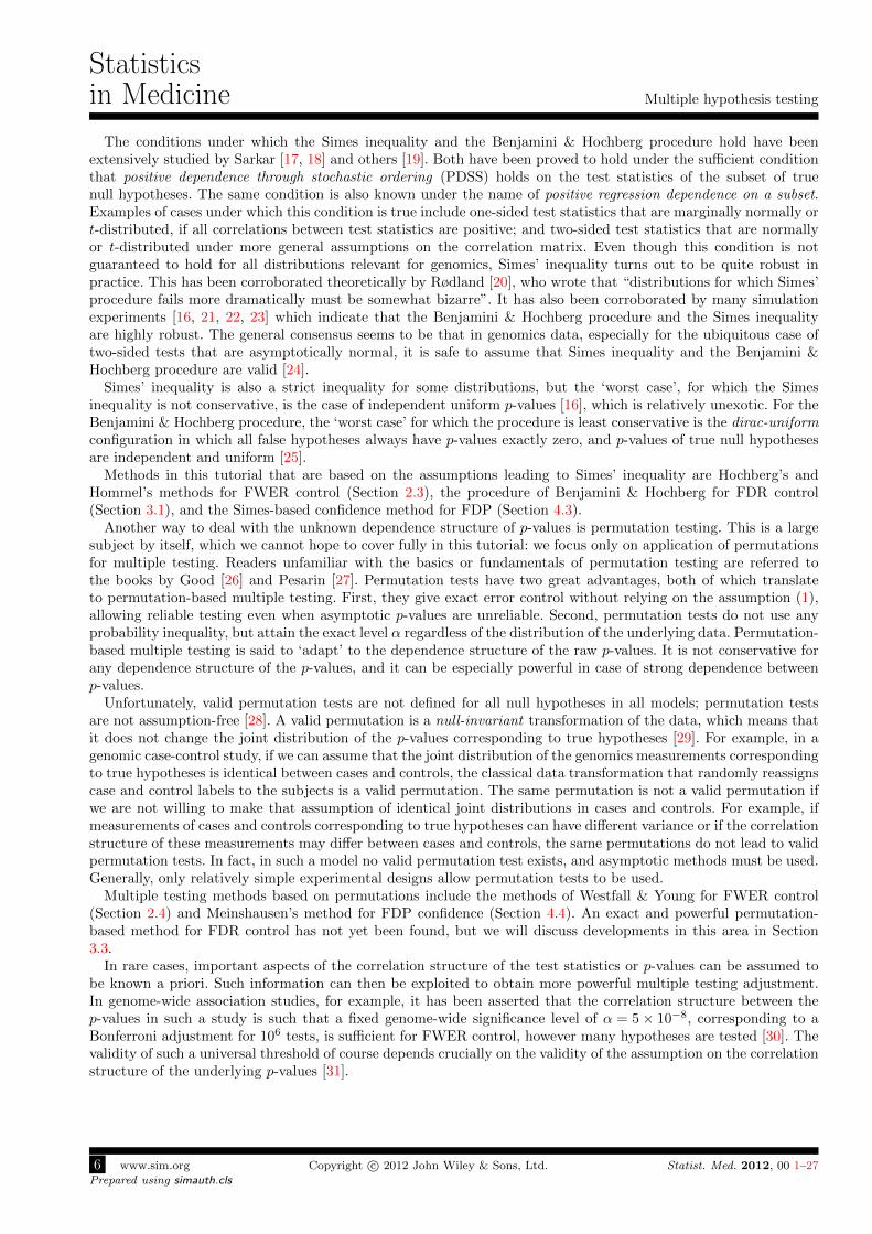
In each data set we performed a likelihood ratio test in a Cox proportional hazards model for each probe, testingassociation of expression with survival. The plot of the sorted p-values and a histogram of the p-values are givenin Figure 1. From the left-hand plot we may suspect that many of the hypotheses that are tested in the Van deVijver data are false. If the overwhelming majority of the hypotheses were true, we would expect the histogram ofthe p-values to be approximately uniform and the plot of the sorted p-values approximately to follow the dottedline, because p-values of true null hypotheses follow a uniform distribution. There is less immediate evidence fordifferential expression in the Rosenwald data, although there seems to be enrichment of low p-values here too. Beforejumping to conclusions, however, it should be noted that, although we expect uniform profiles for the p-values oftrue null hypotheses on average, correlations between p-values can make figures such as the ones in Figure 1 highlyvariable. Without further analysis, it is not possible to attribute the deviations from uniformity in these plotsconfidently to the presence of false hypotheses.
1.6. Available software
Since R is the dominant statistical software package for the analysis of genomics data, we concentrate on availablepackages for that program. Some of the less complex methods can easily be perfomed ‘by hand’ in a spreadsheet,and we summarize these methods in the box of Algorithm 1. A single useful and user-friendly suite of methodsfor multiple testing that encompasses many more methods than we can discuss here is available though the Rpackage of the µTOSS project [34]. For those who do not use R, SAS also has a large collection of multiple testingprocedures. Multiple testing in other commercial packages such as SPSS and Stata is, unfortunately, very limited.
2. Methods for FWER control
The traditional and most well-known method to control FWER is the method of Bonferroni, which replaces thecut-off α for declaring significance of individual tests by α/m. Despite being so well-known, or perhaps because ofthis, there is a lot of misunderstanding about the method of Bonferroni in the literature. We will start this sectionwith a discussion of these misunderstandings, before we move on to the more powerful methods of Holm, Hochberg,Hommel and Westfall & Young.
2.1. Bonferroni
One of the most widespread misunderstandings of the method of Bonferroni is that it would be based on anassumption of independence between p-values [35]. Indeed, the probability of making a false rejection if all m0
p-values of true null hypotheses are independent, and we perform each test at level α/m is 1− (1− α/m)m0 .Expanding this expression, the first term, which is dominant for small α or large m, is m0α/m ≤ α. This reasoning,often presented as motivation for the Bonferroni procedure, does not do it justice. It makes Bonferroni seem likea method that only provides approximate FWER control, and that requires an assumption of independence for itsvalidity.
In fact, the Bonferroni method is a corollary to Boole’s inequality, which says that for any collection of eventsE1, . . . , Ek, we have
P( k⋃i=1
Ei)≤
k∑i=1
P(Ei).
It follows from Boole’s inequality together with (1) that, if q1, . . . , qm0are the p-values of the true null hypotheses,
that the probability that there is some i for which qi ≤ α/m is given by
P(
miniqi ≤ α/m
)= P
( m0⋃i=1
{qi ≤ α/m})≤
m0∑i=1
P(qi ≤ α/m) ≤ m0α
m≤ α. (4)
Statist. Med. 2012, 00 1–27 Copyright c© 2012 John Wiley & Sons, Ltd. www.sim.org 7Prepared using simauth.cls

Statisticsin Medicine Multiple hypothesis testing
p−value
Fre
quen
cy
0.0 0.2 0.4 0.6 0.8 1.0
020
040
060
080
010
0012
00
0 1000 2000 3000 4000 5000
0.0
0.2
0.4
0.6
0.8
1.0
rank of p−value
p−va
lue
(a) Van de Vijver data
p−value
Fre
quen
cy
0.0 0.2 0.4 0.6 0.8 1.0
010
020
030
040
050
0
0 2000 4000 6000
0.0
0.2
0.4
0.6
0.8
1.0
rank of p−value
p−va
lue
(b) Rosenwald data
Figure 1. Histogram and profile of p-values from the data sets of Van de Vijver and Rosenwald.
A few things can be learnt from this derivation. In the first place, the FWER control of Bonferroni is exact, notapproximate, and it is valid for all dependence structures of the underlying p-values. Secondly, the three inequalitiesin (4) indicate in which cases the Bonferroni method can be conservative. The right-hand one shows that Bonferronidoes not control the FWER at level α but actually at the stricter level π0α, where π0 = m0/m. If there are manyfalse null hypotheses, Bonferroni will be conservative. The middle inequality, that uses (1), says thay Bonferroni isconservative if the raw p-values are. The left-hand inequality is due to Boole’s law. This inequality is a strict one inall situations except the one in which all events {qi ≤ α/m} are disjoint. From this, we conclude that Bonferroni isconservative in all situations except in the situation that the rejection events of the true hypotheses are perfectlynegatively associated.
The conservativeness of Bonferroni in situations in which Boole’s inequality is strict deserves more detailedattention. With independent p-values, this conservativeness is present but very minor. To see this we can comparethe Bonferroni critical value α/m with the corresponding Sidak [36] critical value 1− (1− α)1/m for independentp-values. For m = 5 and α = 0.05 we find a critical value of 0.01021 for Sidak against 0.01 for Bonferroni. Asm increases, the ratio between the two increases to a limit of − log(1− α)/α, which evaluates to only 1.026 for
8 www.sim.org Copyright c© 2012 John Wiley & Sons, Ltd. Statist. Med. 2012, 00 1–27
Prepared using simauth.cls
Multiple hypothesis testing
Statisticsin Medicine
α = 0.05. Much more serious conservativeness can occur if p-values are positively correlated. For example, in theextreme case that all p-values are perfectly positively correlated, FWER control could already have been achievedwith the unadjusted level α, rather than α/m. Less extreme positive associations between p-values would also allowless stringent critical values, and Bonferroni can be quite conservative in such situations.
A second, less frequent misunderstanding about Bonferroni is that it would only protect in the situation of theglobal null hypotheses, i.e. the situation that m0 = m [35, 37]. This type of control is known as weak FWERcontrol. On the contrary, as we can see from (4) Bonferroni controls the FWER for any combination of true andfalse hypotheses. This is known a strong FWER control. In practice, only strong FWER controlling methods are ofinterest, and methods with only weak control should, in general, be avoided. To appreciate the difference betweenweak and strong control, consider a method that, if there is at least one p-value below α/m, rejects all m hypotheses,regardless of the p-values they have. This nonsensical method has weak, but not strong FWER control. Related toweak control methods but less overconfident are global testing methods [38, 39] that test the global null hypothesisthat m0 = m. If such a test is significant, one can confidently make the limited statement that at least one falsehypotheses is present, but not point to which one. In contrast, methods with strong FWER control also allowpinpointing of the precise hypotheses that are false.
When testing a single hypothesis, we often do not only report whether a hypothesis was rejected, but also thecorresponding p-value. By definition, the p-value is the smallest chosen α-level of the test at which the hypothesiswould have been rejected. The direct analogue of this in the context of multiple testing is the adjusted p-value,defined as the smallest α level at which the multiple testing procedure would reject the hypothesis. For the Bonferroniprocedure, this adjusted p-value is given by min(mpi, 1), where pi is the raw p-value.
2.2. Holm
Holm’s method [40] is a sequential variant of the Bonferroni method that always rejects at least as much asBonferroni’s method, and often a bit more, but still has valid FWER control under the same assumptions. Fromthis perspective, there is no reason, aside from possibly simplicity, to use Bonferroni’s method in preference toHolm’s.
Holm remedies part of the conservativeness in the Bonferroni method arising from the right-hand inequality of(4), which makes Bonferroni control FWER at level π0α. It does that by iterating the Bonferroni method in thefollowing way. In the first step, all hypotheses with p-values at most α/h0 are rejected, with h0 = m just like inthe Bonferroni method. Suppose this leaves h1 hypotheses unrejected. Then, in the next step, all hypotheses withp-values at most α/h1 are rejected, which leaves h2 hypotheses unrejected, which are subsequently tested at levelα/h2. This process is repeated until either all hypotheses are rejected, or until a step fails to result in any additionalrejections. Holm gave a very short and elegant proof that this procedure controls the FWER in the strong sense atlevel α. This proof is based on Boole’s inequality just like that of the Bonferroni method, and consequently makesno assumptions whatsoever on the dependence structure of the p-values.
It is immediately obvious that Holm’s method rejects at least as much as Bonferroni’s and possibly more. Thegain in power is greatest in the situation that many of the tested hypotheses are false, and when power for rejectingthese hypotheses is good. Rejection of some of these false hypotheses in the first few steps of the procedure maylead to an appreciable increase in the critical values for the remaining hypotheses. Still, unless the proportion offalse hypotheses in a testing problem is very large, the actual gain is often quite small. We can see this in theexample data sets of Rosenwald and Van de Vijver. In de Van de Vijver data, the Bonferroni method rejects203 hypotheses at a critical value of 0.05/4919 = 1.02× 10⁻⁵. This allows the critical value in the second stepof Holm’s procedure to be adjusted to 0.05/4716 = 1.06× 10⁻⁵, which allows 3 more rejections. The increase inthe critical value resulting from these three rejections is not sufficient to allow any additional rejections, givinga total of 206 rejections for Holm’s procedure. In the Rosenwald data, Bonferroni allows only 4 rejections at itscritical value of 0.05/7399 = 6.76× 10⁻⁶, but the resulting increase in the critical value in Holm’s method to0.05/7395 = 6.76× 10⁻⁶ is insufficient to make a difference.
An alternative way of describing Holm’s method is via the ordered p-values p(1), . . . , p(m). Comparing each p-valuep(i) to its corresponding critical value α/(m− i+ 1), Holm’s method finds the smallest j such that p(j) exceedsα/(m− j + 1), and subsequently rejects all j − 1 hypotheses with a p-value at most α/(m− j). If no such j can befound, all hypotheses are rejected.
Adjusted p-values for Holm’s method can be calculated using the simple algorithm of Table 1. Because increasingthe level of α, when this causes one rejection, may immediately trigger a second one because of the resulting increasein the critical value, it is possible for adjusted p-values in Holm’s method to be equal to each other even when theraw p-values are not. The same feature occurs in almost all of the other methods described below.
Statist. Med. 2012, 00 1–27 Copyright c© 2012 John Wiley & Sons, Ltd. www.sim.org 9Prepared using simauth.cls

Statisticsin Medicine Multiple hypothesis testing
Start with p-values for m hypotheses
1. Sort the p-values p(1), . . . , p(m).2. Multiply each p(i) by its adjustment factor ai, i = 1, . . . ,m, given by
(a) Holm or Hochberg : ai = m− i+ 1(b) Benjamini & Hochberg : ai = m/i(c) Benjamini & Yekutieli : ai = lm/i, with l =
∑mk=1 1/k
3. If the multiplication in step 2 violate the original ordering, repair this.
(a) Step-down (Holm): Increase the smallest p-value in all violating pairs:
p(i) = maxj=1,...,i
ajp(j)
(b) Step-up (all others): Decrease the highest p-value in all violating pairs:
p(i) = minj=i,...,m
ajp(j)
4. Set p(i) = min(p(i), 1) for all i.
Algorithm 1: Calculating adjusted p-values for the methods of Holm, Hochberg, Benjamini & Hochberg (BH), andBenjamini & Yekutieli (BY). The algorithms above are easy to implement in any spreadsheet program. In R, it iseasier to just use the p.adjust function, which also has Hommel’s method.
2.3. Hochberg and Hommel
Bonferroni’s and Holm’s methods make no assumptions on the dependence structure of the p-values, and protectagainst the ‘worst case’ according to Boole’s inequality, which is that the rejection regions of the different tests aredisjoint. If we are willing to make assumptions on the joint distribution of the p-values, it becomes possible excludethis worst case a priori, and as a result gain some power.
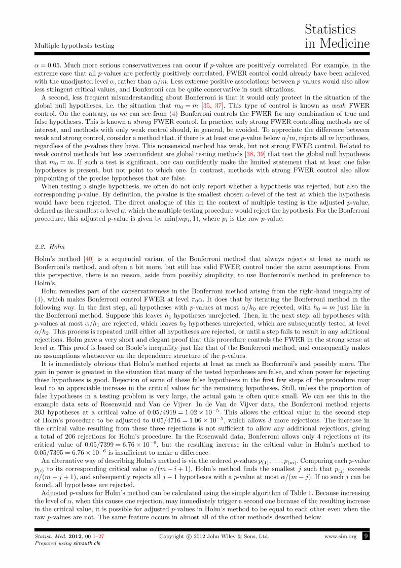
One such assumption could be that the PDSS condition holds for the subset of true hypotheses (Section 1.4).This assumption makes the use of Simes inequality (3) and therefore the use of Hochberg’s method [41] possible,which is very similar to Holm’s method but more powerful. Hochberg’s method (not to be confused with Benjamini& Hochberg’s method, Section 3) compares each ordered p-value p(i) to a critical value α/(m− i+ 1), the sameas Holm’s. It then finds the largest j such that p(j) is smaller than α/(m− j + 1), and subsequently rejects allj hypotheses with p-values at most α/(m− j + 1). In the jargon of multiple testing methods, Holm’s method isknown as a step-down method and Hochberg’s as its step-up equivalent. An illustration of the difference betweenstep-up and step-down methods is given in Figure 2. Holm’s method uses the first crossing point between the p-valuecurve p(1), . . . , p(m) and the critical value curve α/m,α/(m− 1), . . . , α as its critical value, while Hochberg’s usesthe largest crossing point instead. The step-up/step-down parlance can be somewhat confusing, as Holm’s method“steps up” from the smallest p-value to find the crossing while Hochberg’s “steps down” from the largest one, butthe terminology was originally formulated in terms of test statistics rather than p-values. Comparing to Holm’smethod, it is clear that Hochberg’s method rejects at least as much as Holm’s method, and possibly more. If thep-value and critical value curves never cross or only once, Holm’s and Hochberg’s methods reject the same numberof hypotheses. If the same curves cross multiple times or if the smallest p-value is larger than its correspondingcritical value, Hochberg’s method rejects more.
Hochberg’s method is a special case of the powerful closed testing procedure [42], and the proof of its FWERcontrol is based on combining that procedure with the Simes inequality. Hommel [43] showed that a more powerful,although more complicated and computationally more demanding procedure can be constructed from the sameingredients. Hommel’s resulting procedure rejects at least as much as Hochberg’s, but possibly more [44]. Onmodern computers the additional computational burden of Hommel’s procedure is not an impediment anymore,and Hommel’s procedure should always be preferred to Hochberg’s just like Holm’s procedure should always bepreferred to Bonferroni’s.
A gain in power of Hochberg’s and Hommel’s methods over Holm’s method can be expected in the situation thata large proportion of the hypotheses is false, but the corresponding tests have relatively low power, or if there arepositive associations between the p-values of these false hypotheses. In practice, just like the gain from Bonferronito Holm’s method, the number of additional rejections allowed by Hochberg or Hommel is often small. In the Van
10 www.sim.org Copyright c© 2012 John Wiley & Sons, Ltd. Statist. Med. 2012, 00 1–27
Prepared using simauth.cls

Multiple hypothesis testing
Statisticsin Medicine
de Vijver data set, the curve of the ordered p-values crosses the curve of the Holm and Hochberg critical valuesonly once, so the number of rejections is identical to 206 in both methods. Hommel’s method, however, is able toimprove upon this by a further three rejections, making a total of 209. In the Rosenwald data, neither method isable to improve upon the 4 rejections that were already found by the Bonferroni procedure.
The algorithm for calculating adjusted p-values in Hochberg’s method is given in Table 1. For Hommel’s methodthis calculation is less straightforward, and we refer to the p.adjust function in R. Step-up methods tend to givemore tied adjusted p-values than step-down ones, and may sometimes return long lists of identical adjusted p-values.
Figure 2. Comparison of rejections by step-up and step-down methods with the same critical values. The dots are observed ranked p-values.
The line represents the critical values. Step-down methods reject all hypotheses up to, but not including, the first p-value that is larger than
its critical value. Step-up methods reject all hypotheses up to and including the last p-value that is smaller than its critical value.
1
rejected by a step-up method
rejected by a step-down method
1 2 3 4 5 6 7 8 90
rank of p-value
p-v
alu
e
2.4. Permutations and Westfall & Young
Instead of making assumptions on the dependence structure of the p-values, it is also possible to adapt the procedureto the dependence that is observed in the data by replacing the unknown true null distribution with a permutationnull distribution. In FWER control, the most relevant aspect of the unknown null distribution is the α-quantile ofthe distribution of the minimum p-value of the m0 true hypotheses. This is the quantile that Bonferroni boundsfrom below by α/m. The method of Westfall & Young [45] uses permutations to obtain a more accurate threshold.It isshown to be asymptotically optimal for a broad class of correlation structures [46]. Two variant’s of Westfall &Young’s methods exist: the maxT and minP methods.
In the Van de Vijver or Rosenwald data, a permutation can be a reallocation of the survival time and status tothe subjects, so that each subject’s gene expression vector now belongs to the survival time of a different subject.For the probes for which there is no association between survival time and gene expression, we can assume thedistribution of this permuted data set to be identical to that of the original, thus satisfying the null invariancecondition. Since permutation-testing is not assumption-free, it is important to check carefully that permutationsare indeed valid. If an additional covariate would be present in the Cox proportional hazards model, for example,the survival curves would not have been identical between individuals, and null invariance would have been muchmore problematic. In situations in which null invariance is not satisfied, simple per-hypothesis permutation testingcombined with Holm’s or Hommel’s method can sometimes be an alternative to Westfall & Young.
Practically, the maxT method of Westfall & Young, applied to the p-values, starts by making k permuted datasets, and recalculating all m p-values for each permuted data set. Let’s say we store the results in an m× k matrixP. We find the k minimal p-values along each column to obtain the permutation distribution of the minimump-value out of m. The α-quantile α0 of this distribution is the permutation-based critical value, and Westfall &Young reject all hypotheses for which the p-value in the original data set is strictly smaller than α0. Next, we maycontinue from this result in the same step-down way in which Holm’s method continues on Bonferroni’s. In the
Statist. Med. 2012, 00 1–27 Copyright c© 2012 John Wiley & Sons, Ltd. www.sim.org 11Prepared using simauth.cls

Statisticsin Medicine Multiple hypothesis testing
next step we may remove from the matrix P all rows corresponding to the hypotheses rejected in the first step,and recalculate the k minimal p-values and their α-quantile α1. Removal of some hypotheses may have increasedthe values of some of the minimal p-values, so that possibly α1 > α0. We may now reject any additional hypothesesthat have p-values below the new quantile α1. The process of removing rows of rejected hypotheses from P andrecalculating the α-quantile of the minimal p-values is repeated until any step fails to result in additional rejections,or until all hypotheses have been rejected, just like in Holm’s procedure.
Westfall & Young’s minP method is similar to the maxT method, except that instead of the raw p-values it usesthe per-hypothesis permutation p-values in the matrix P. A fast algorithm for this procedure was designed by Ge[47]. Since permutation p-values take only a limited number of values, the matrix P will always contain many tiedvalues, which is an important practical impediment for the minP method, as we’ll see below.
The number permutations is always an issue with permutation-based multiple testing. In data with a smallsample size this number is necessarily be limited, but it quickly becomes very large already for moderate datasets. Although it would be best to use the collection of all possible permutations, this is often computationally notfeasible, so a collection of randomly generated permutations is often used. Additional randomness is introduced inthis way, which makes rejections and adjusted p-values random, especially if only few random permutations areused. The minimum number of permutations required depends on the method, the α-level, and on the presence ofrandomness in the permutations. The maxT method requires fewest permutations, and can work well with only1/α permutations, whatever the value of m, if p-values are continuous and all permutations can be enumerated.With random permutations a few more permutations are recommended to suppress randomness in the results, but anumber of 1,000 permutations is usually quite sufficient at α = 0.05, whatever m. The minP method requires manymore permutations. Because of the discreteness of the permutation p-values, the minimum observed p-value will beequal to the minimum possible p-value for most of the permuted data sets unless the number of permutationsis very large, resulting in zero power for the method. For the minP procedure, therefore, we recommend touse m/α permutations as an absolute minimum, but preferably many more. Such numbers of permutations arecomputationally prohibitive for typical values of m. Similar numbers of permutations are necessary for combinationsof per-hypothesis permutation testing with Holm’s or Hommel’s procedure.
In the Van de Vijver data set we shuffled the survival status of the subjects 1,000 times, created a 4, 919× 1, 000matrix P of p-values, and performed the maxT procedure. The α-quantile of the distribution of the minimump-values is found at 1.08× 10⁻⁵, which is remarkably close to the Bonferroni threshold of 1.02× 10⁻⁵, but stillleads to 4 more rejections, for a total of 207. Stepping down by removing the rejected hypotheses leads to a slightrelaxation of the threshold and one additional rejection, for a total of 208 rejections. In the Rosenwald data, theα-quantile of the minimum p-values evaluates to 7.86× 10⁻⁶, which is higher than the threshold of to 6.76× 10⁻⁶
for Bonferroni, but does not lead to more rejections. Removal of the 4 rejected hypotheses does not alter theα-quantile, so the method stops at 4 rejections.
A gain in power for Westfall & Young’s maxT method relative to Holm or Hommel can be achieved with Westfall& Young especially if strong positive correlations between p-values exist. The permutation method will adaptto the correlation structure found in the data, and does not have to take any worst case into account. A gainin power may also occur if the raw p-values are conservative. Permutation testing does not use the fact that p-values of true hypotheses are uniformly distributed, but adapts to the actual p-value distribution just as it adaptsto the true correlation structure. Use of Westfall & Young does not require blind faith in the accuracy of theasymptotics underlying the raw p-values. Where methods that are not permutation-based become conservative oranti-conservative with the underlying raw p-values, Westfall & Young can even work with invalid and possiblyanti-conservative p-values calculated from an incorrect model, and produce correct FWER control on the basis ofsuch p-values. Although this sounds fabulous, it is sensible to be careful with this, however, since p-values frominvalid models tend to be especially wild for probes for which the model fits badly, rather than for probes withan interesting effect. For this reason the power of a Westfall & Young maxT procedure based on such p-valuesis often disappointing. The minP variant of the Westfall & Young procedure partially mends this by working onthe per-probe permutation p-values instead of the raw p-values, guaratneeing a uniform distribution of the inputp-values for the method.
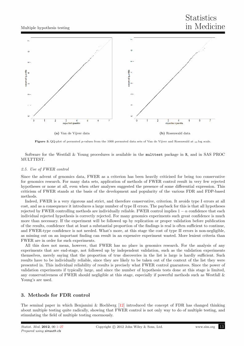
In the case of the Van de Vijver and Rosenwald data, the asymptotic distribution of the p-values seems to holdreasonably well, as can be seen in Figure 3, a QQ-plot of the 10 log of all the permuted p-values, although a slighttendency to anti-conservatism is noticeable in the Van de Vijver data. Such anti-conservatism would make themethods from previous sections anti-conervative, but has no effect on the Westfall & Young method.
Adjusted p-values can be easily calculated for the Westfall & Young procedure. They are always a multiple of1/(k + 1) for random permutations, or of 1/k if all permutations can be enumerated [48]. For random permutations,letting α range over 1/(k + 1), 2/(k + 1), . . . , 1, and adjusting the α-quantile of the minimum p-value distributionaccordingly, we can easily find the smallest of these α-levels that allows rejection of each hypothesis.
12 www.sim.org Copyright c© 2012 John Wiley & Sons, Ltd. Statist. Med. 2012, 00 1–27
Prepared using simauth.cls
Multiple hypothesis testing
Statisticsin Medicine
(a) Van de Vijver data (b) Rosenwald data
Figure 3. QQ-plot of permuted p-values from the 1000 permuted data sets of Van de Vijver and Rosenwald at 10 log scale.
Software for the Westfall & Young procedures is available in the multtest package in R, and in SAS PROCMULTTEST.
2.5. Use of FWER control
Since the advent of genomics data, FWER as a criterion has been heavily criticised for being too conservativefor genomics research. For many data sets, application of methods of FWER control result in very few rejectedhypotheses or none at all, even when other analyses suggested the presence of some differential expression. Thiscriticism of FWER stands at the basis of the development and popularity of the various FDR and FDP-basedmethods.
Indeed, FWER is a very rigorous and strict, and therefore conservative, criterion. It avoids type I errors at allcost, and as a consequence it introduces a large number of type II errors. The payback for this is that all hypothesesrejected by FWER controlling methods are individually reliable. FWER control implies 1− α confidence that eachindividual rejected hypothesis is correctly rejected. For many genomics experiments such great confidence is muchmore than necessary. If the experiment will be followed up by replication or proper validation before publicationof the results, confidence that at least a substantial proportion of the findings is real is often sufficient to continue,and FWER-type confidence is not needed. What’s more, at this stage the cost of type II errors is non-negligible,as missing out on an important finding can result in an expensive experiment wasted. More lenient criteria thanFWER are in order for such experiments.
All this does not mean, however, that FWER has no place in genomics research. For the analysis of anyexperiments that are end-stage, not followed up by independent validation, such as the validation experimentsthemselves, merely saying that the proportion of true discoveries in the list is large is hardly sufficient. Suchresults have to be individually reliable, since they are likely to be taken out of the context of the list they werepresented in. This individual reliability of results is precisely what FWER control guarantees. Since the power ofvalidation experiments if typically large, and since the number of hypothesis tests done at this stage is limited,any conservativeness of FWER should negligible at this stage, especially if powerful methods such as Westfall &Young’s are used.
3. Methods for FDR control
The seminal paper in which Benjamini & Hochberg [12] introduced the concept of FDR has changed thinkingabout multiple testing quite radically, showing that FWER control is not only way to do of multiple testing, andstimulating the field of multiple testing enormously.
Statist. Med. 2012, 00 1–27 Copyright c© 2012 John Wiley & Sons, Ltd. www.sim.org 13Prepared using simauth.cls

Statisticsin Medicine Multiple hypothesis testing
Compared to FWER control, the subject of FDR control is relatively young. Much method-development is stillongoing, and some important questions are still partially open. This holds especially for the complicated situationof dependent p-values that is so important for applications in genomics research. In this paper, we leave aside theextensive literature on FDR control for independent p-values, and focus only on results that are known or believedto be valid under fairly general forms of dependence. We follow the same structure as for FWER-based methods,discussing methods that are generally valid, methods valid under the assumption that Simes inequality holds, andmethods based on permutations. For FDR, unlike for FWER, the Simes-based method is the oldest and best knownone, so we start there.
3.1. Benjamini & Hochberg
The Benjamini & Hochberg procedure [12] is a step-up procedure just like the Hochberg procedure, only with highercritical values. It compares each ordered p-value p(i) with the critical value iα/m, finds the largest j such that p(j)
is smaller than its corresponding critical value, and rejects the j hypotheses with the j smallest p-values. TheBenjamini & Hochberg method is closely related to Simes’ inequality (3), and the critical values of the Benjamini& Hochberg procedure are those of Simes’ inequality with m = m0.
It has been shown that this procedure controls FDR at level α if the PDSS assumption holds on the subset oftrue hypotheses [19]. This is the same assumption that underlies Simes inequality and Hochberg’s and Hommel’smethods. The Benjamini & Hochberg procedure has valid FDR control if the test statistics underlying the p-valuesare positively correlated for one-sided tests, or under more general dependence structures for two-sided tests. Asdiscussed in Section 1.4, the validity of the procedure seems quite robust, at least for two-sided tests that areasymptotically normal. In fact, control of FDR under these assumptions is even at level π0α, where π0 = m0/m,rather than at level α.
The critical values of the Benjamini & Hochberg procedure are much larger than those of Hochberg or Hommel, sothat many more rejections can often be made. In the Van de Vijver data, 1,340 hypotheses with p-values below 0.0136are rejected at an FDR of 0.05, compared to 206 with p-values below 1.06× 10⁻⁵ for Hochberg’s method. In theRosenwald data we reject 72 hypotheses with p-values below 4.86× 10⁻⁴ with Benjamini & Hochberg, comparedwith 4 with p-values below 6.76× 10⁻⁶ for Hochberg. Clearly, without changing the assumptions, relaxing thecriterion from FWER to FDR can make a huge difference in terms of power.
A gain in power of Benjamini & Hochberg’s method relative to Hochberg’s, and in general of FDR-based versusFWER-based methods is most pronounced when many false hypotheses are present. This can be understood bycomparing the FDR and FWER criteria. In FDR, the more hypotheses are rejected, the higher the denomimatorof the false discovery proportion Q, and the less stringent the error criterion for the next rejection becomes.
The Benjamini & Hochberg method, like Bonferroni, controls its error rate at level π0α, rather than at α. Thissuggests the possibility an alternative, more powerful Benjamini & Hochberg procedure that uses critical valuesiα/(π0m) rather than iα/m if a good estimate π0 of π0 would be available. Such a procedure might have an FDRcloser to the chosen level α, and would be even more powerful than the original procedure if many hypotheses werefalse. Such procedures are called adaptive procedures, and many have been proposed based on various estimates ofπ0 [49]. A problem with the adaptive approach, however, is that estimates of π0 can have high variance, especiallyif p-values are strongly correlated. Naive plug-in procedures, in which this variance is not taken into account, willtherefore generally not have FDR control, especially if π0 ≈ 1. More sophisticated methods are needed that dotake the estimation error of π0 into account. One such procedure, by Benjamini, Krieger and Yekutieli [50], adjuststhe α-level slightly from α to α∗ = α/(1 + α) to adjust for the additional variance from estimation of π0. Thisprocedure estimates π0 by first performing an initial Benjamini & Hochberg procedure at the slightly reduced levelα∗, estimating π0 by π0 = (m−R0)/m, where R0 is the number of rejections obtained in this first step. In thesecond and final step, a subsequent Benjamini & Hochberg procedure is done at level α∗/π0. Note that, unlikesimpler plug-in procedures, this latter procedure is not guaranteed to give more rejections than the regular, non-adaptive Benjamini & Hochberg procedure, since α∗/π0 may be smaller than α. This reflects the additional riskincurred in estimating π0. The adaptive procedure estimates π0 = 0.73 for the Van de Vijver data, resulting in1,468 rejections, compared to 1,340 for the non-adaptive procedure. In the Rosenwald data the same procedurefinds a disappointing π0 = 0.99, so that the critical value for the second stage is increased rather than decreased. Anumber of 69 hypotheses are rejected, compared to 72 for the non-adaptive Benjamini & Hochberg procedure. FDRcontrol for the adaptive Benjamini, Krieger and Yekutieli procedure has only yet been proven under independence,although simulations suggest FDR control under positive dependence as well [50, 23, 51]. In any case, adaptiveprocedures are expected to have increased power over the ordinary Benjamini & Hochberg procedure only of theproportion π0 of true null hypotheses is substantially smaller than 1. If π0 is near 1, the power of such proceduresis often worse. From a practical perspective, sacrificing power for the case that π0 is near 1 in favor of power for
14 www.sim.org Copyright c© 2012 John Wiley & Sons, Ltd. Statist. Med. 2012, 00 1–27
Prepared using simauth.cls
Multiple hypothesis testing
Statisticsin Medicine
small values of π0 is seldom desirable: it increases the risk of not getting any rejections for poor data sets, whileincreasing the number of rejections in data sets in which there are already many rejections.
In Section 1.3 we argued that FDR control does not necessarily imply per comparison type I error control forindividual hypotheses, and that procedures may sometimes reject hypotheses with p-values above α. The Benjamini& Hochberg method never does this, but adaptive variants might.
As a side note, we remark that adaptive control is not unique to FDR, and plug-in Bonferroni methods have alsobeen suggested [52]. Just like for plug-in FDR, however, no proof of FWER control for such methods is availableexcept under strong assumptions on the dependence structure of p-values.
Adjusted p-values for the procedure of Benjamini & Hochberg can be calculated using Algorithm 1. Adjustedp-values for FDR are sometimes referred to as q-values, but use of this term remains mostly connected to Storey’smethods (Section 4.1). Some care must be applied when interpreting adjusted p-values based on FDR control,however, as we’ll discuss in Section 3.4.
3.2. FDR control under general dependence
The equivalent to the Benjamini & Hochberg procedure that is valid even when the conditions for Simes’ inequalitydoes not hold is the procedure of Benjamini & Yekutieli [19]. This procedure is linked to Hommel’s variant (2) ofthe Simes inequality in the same way that the procedure of Benjamini & Hochberg is linked with Simes inequality(3) itself. It is a step-up procedure that compares each ordered p-value p(i) with the critical value iα/(m
∑mj=1 1/j),
finds the largest j such that p(j) is smaller than its corresponding critical value, and rejects the j hypotheseswith the j smallest p-values. Like Hommel’s inequality relative to Simes, the Benjamini & Yekutieli procedure ismore conservative than the Benjamini & Hochberg procedure by a factor
∑mj=1 1/j. Like Hommel’s inequality, the
Benjamini & Yekutieli procedure is valid under any dependence structure of the p-values. Adjusted p-values for theBenjamini & Yekutieli method can be calculated using Algorithm 1.
The method of Benjamini & Hochberg is guaranteed to reject at least as much as Hochberg’s procedure, which usesthe same assumptions but controls FWER rather than FDR. The same does not hold for the method of Benjamini& Yekutieli relative to Holm’s method, which is the standard method for FWER control under any dependence ofthe p-values. We see this immediately when we apply the Benjamini & Yekutieli procedure on the example datasets. In the Rosenwald data, where Holm’s method rejected 4 hypotheses and Benjamini & Hochberg rejected 72,the procedure of Benjamini & Yekutieli, which effectively performs the Benjamini & Hochberg procedure at a levelα/(∑m
j=1 1/j), which evaluates to 5.27× 10⁻³, allows no rejections at all. Comparing critical values, we see that
the first log(m) critical values of Holm’s method are larger than the corresponding critical values of Benjamini &Yekutieli. Therefore, if the expected number of false hypotheses is very small, Holm’s method may be superior interms of power to Benjamini & Yekutieli, and a better choice for FDR control. For less than extremely sparse data,however, we can expect Benjamini & Yekutieli to be more powerful than Holm. In the Van de Vijver data, wherem is smaller and there are more false hypotheses, Benjamini & Yekutieli do reject substantially more than Holm,namely 614 hypotheses against 206 for Holm.
Alternatives to the Benjamini & Yekutieli method have been formulated by Sarkar [18] and by Blanchard andRoquain [53]. The latter authors proved that any step-up method with critical values of the form
ci =α
m
i∑j=1
jfj , (5)
for non-negative constants f1, . . . , fm such that∑m
j=1 fj = 1, has control of FDR for any dependence struture of the
p-values. Taking fj = 1/(j∑m
k=1 1/k) retrieves the Benjamini & Yekutieli critical values. Taking fj = 1/m retrievesthe critical values proposed by Sarkar [18], given by
ci =i(i+ 1)α
2m2.
Sarkar’s method rejects 454 hypotheses in the Van de Vijver data, which is less than the method of Benjamini& Yekutieli. In the Rosenwald data, Sarkar’s method, like Benjamini & Yekutieli, gives no rejections. A wholerange of other FDR-controlling procedures also becomes possible in this way, parameterized by any chosen valuesof f1, . . . , fm. As a motivation for choosing these values, it is helpful to realize that high values of fj for some jmake it relatively more likely that exactly j hypotheses will be rejected by the procedure [53]. From this, it is clearthat Sarkar’s method, even more than the method of Benjamini & Yekutieli, is focused on the situation that manyhypotheses are false. No choice of f1, . . . , fm leads to an FDR controlling method that always rejects at least as muchas Holm’s method. As far as is currently known, therefore, also Holm’s method remains admissible for controlling
Statist. Med. 2012, 00 1–27 Copyright c© 2012 John Wiley & Sons, Ltd. www.sim.org 15Prepared using simauth.cls

Statisticsin Medicine Multiple hypothesis testing
FDR under general dependence, and it has the added boon of also controlling FWER. Still, Holm’s method is onlyexpected to be superior to Benjamini & Yekutieli in the situation that the number of false hypotheses is at mostof the order of magnitude of log(m), so that π0 ≈ 1. In all other situations, the method of Benjamini & Yekutieliis a better choice.
3.3. FDR control by resampling
Several authors have worked on FDR control by permutation or by other types of resampling such as the bootstrap.However, an FDR controlling method with the power, simplicity and reliability of the method of Westfall & Young(Section 2.4) has not yet been found.
Research in this area is ongoing. The subject was pioneered by Yekutieli and Benjamini [54] who suggested apermutation-based procedure but without full proof of FDR control. Romano, Shaikh and Wolf [55], building onearlier work by Troendle [56] that had restrictive parametric assumptions, proposed a method use the bootstrapinstead of permutations to control FDR asymptotically. Ge, Sealfon and Speed [57] proposed three different FDR-controlling methods, one of which has proven finite-sample FDR control. Its assumptions are more restrictive thanthose of the familywise error controlling method of Westfall & Young, but the method is still only marginallymore powerful than that method, rejecting 209 hypotheses in the Van de Vijver data, one more that Westfall &Young, and 4 in the Rosenwald data, like Westfall & Young. None of the permutation FDR methods comes withuser-friendly software.
3.4. Use of FDR control
As we have seen from the example data, FDR control is usually much less conservative than FWER control. Controlof FDR, since that criterion is concerned with the proportion of type I errors among the selected set, is more suitablefor exploratory genomics experiments than FWER control. FDR control methods do a very good job in selectinga set of hypotheses that is promising, in the sense that we can expect a large proportion of the ensuing validationexperiments to be successful. As a consequence, FDR has effectively become the standard for multiple testing ingenomics. Nevertheless, FDR control has been criticised [58, 59, 60, 61], sometimes heavily [14]. It is helpful toreview some of this criticism in order to understand the properties and the limitations of FDR control better. Twomain points of criticism concern the nature of FDR as an average.
In the first place, FDR is the expected value of FDP, which is a variable quantity because the rejected set R israndom. It has been pointed out, however, that the actual value of FDP realized by FDR-controlling procedures canbe quite variable, especially when p-values are dependent [59]. Sets R found by a method that controls FDR at αoften have an FDP that is much larger than α, or one that is much smaller than α. The realized FDP for a methodcontrolling FDR at 0.05 can, for example, be greater than 0.29 more than 10% of the time [58]. The variability ofFDP around FDR is not taken into account in FDR control methods, and this variability is not quantified. Usersof FDR must be aware that control of FDR at α only controls FDP in expectation, and that the actual proportionof false discoveries in the rejected set can often be substantially larger than α. FDR control is a property of theprocedure leading to a rejected set, not of the rejected set itself.
Secondly, as we have noted in Section 1.3, FDR lacks the subsetting property that FWER does have. If a procedurecontrols FDR, the sets R generated have, on average, a false discovery proportion of maximally α. This propertysays something about the set R, but the does not translate to subsets of R or to specific individual hypothesesthat are elements of R [14]. Subsets may have much higher false discovery proportions than the complete set, and,since R is likely to contain a few false positives, each individual hypothesis in R may be such a false positive. Inany case, the fact that R resulted from an FDR controlling procedure does not implicate any properties for subsetsof R. This lack of a subsetting property has several consequences that have to be taken into account when workingwith the results of FDR controlling procedures.
One consequence that has frequently been mentioned is the possibility of ‘cheating’ with FDR [14]. This cheatingcan be done as follows. If a researcher desires to reject some hypotheses using FDR, he or she can greatly increasethe chances of doing so by testing these hypotheses together with a number of additional hypotheses which areknown to be false, and against which he or she has good power. The additional guaranteed rejections alleviate thecritical values for the hypotheses of interest, and make rejection of these hypotheses more likely. The catch of thisapproach is that the resulting FDR statement is about the rejected set including the added hypotheses, and thatno FDR statement may, in fact, be made about the subset of the rejected set that excludes the added hypotheses.The cheating as described above is blatant, of course, and would hardly occur in this way. More often, however,inadvertent cheating of the same type occurs, for example when a list of rejected hypotheses is considered but theobvious, and therefore uninteresting, results are discarded or ignored, when an individual rejected hypothesis issingled out, or when subsets of the rejected hypotheses are considered for biological reasons. If hypotheses are very
16 www.sim.org Copyright c© 2012 John Wiley & Sons, Ltd. Statist. Med. 2012, 00 1–27
Prepared using simauth.cls

Multiple hypothesis testing
Statisticsin Medicine
heterogeneous (e.g. Gene Ontology terms rather than probes) it is difficult not to look at subsets when interpretingthe results on an analysis [61]. For correct interpretation of FDR control results, and to prevent inadvertent cheating,it is important to keep the rejected set complete.
A second consequence of FDR’s lack of the subsets property relates to the interpretation of adjusted p-values. Theadjusted p-value, being the largest α-level at which the hypothesis is rejected by the multiple testing procedure, isusually interpreted as a property of the hypothesis itself. For FWER-adjusted p-values this is warranted, as FWERcontrol for the rejected set implies FWER control for each individual hypothesis within the set. FDR control isdifferent, however: because that is a property of the whole set only, not of individual hypotheses within the set, theadjusted p-value similarly is a property of the whole rejected set, not of any individual hypothesis within that set.It is, therefore, hazardous to interpret such adjusted p-values as properties of individual hypotheses. To see this,consider a hypothesis with an FDR-adjusted p-value just below 0.05. If this hypothesis was the only hypothesisrejected at this α-level, we can be quite confident that this hypothesis is not a type I error. If, on the other hand,20 or more hypotheses were rejected at the same level, the same adjusted p-value does not allow such a clearconclusion about that specific hypothesis. In the extreme, it could be that the top 19 hypotheses are absolutelycertain rejections, and that the 20th hypothesis, even though a type I error with high probability, was added justbecause the FDR level of 0.05 left enough room for an extra rejection. Clearly, because of the lack of the subsettingproperty in FDR, interpreting FDR-adjusted p-values as properties of single hypotheses is problematic. An FDR-adjusted p-value is a property of a rejected set, not of an individual hypothesis. Interpreting it otherwise can beseen as a special case of “cheating with FDR”.
An unrelated property has been shown for FDR can be very advantageous in incremental designs in which dataare being gathered over a long period and repeatedly analyzed ad interim. FWER controlling methods must performall interim analyses and the final analysis at a reduced level to correct for such multiple looks. With FDR, theneed for such corrections all but disappears [62]. Allowing multiple looks, and, conversely, allowing more data tobe added at a later stage after a first analysis, is a very valuable property in exploratory settings.
FDR controlling methods are most useful in exploratory situations in which a promising set of hypotheses mustbe found, and when we are content to use the complete set of hypotheses with top p-values, or something very closeto that set. In such situations these methods are very powerful. If FDR control is used in a final reported analysis,the result of this analysis is the full rejected set, and researchers should be careful when making statements onsubsets or individual hypotheses within that set.
4. Methods for FDP estimation
Next to methods for FDR control there are also methods that approach FDP from an estimation perspective. Itpays to be precise about the quantities that are to be estimated, so we will discuss the difference between FDPestimation and FDR estimation briefly before turning to specific methods.
The purpose of an exploratory genomics experiment is to come up with a set R of discoveries, which are promisingbut might still require validation before they can be publicised. A measure of quality of such a chosen set R is theproportion of type I errors, i.e. the proportion of true null hypotheses present in this specific set, which is given by
q(R) =#(R∩ T )
#R.
For any given set R this quantity is fixed but unknown. The purpose of FDP estimation methods is to come upwith an estimate q(R) for the specific set R that is eventually chosen, and possibly to use the estimates for severalcompeting sets in order to come up with a final choice for R.
In contrast to FDP estimation, FDR estimation aims to estimate FDP on average over the distribution of rejectedsets R induced by the test procedure, rather than for the specific chosen set. FDP is a property of the rejectedset; FDR is a property of the test procedure [60]. The value of FDP depends only on truth and falsehood status ofhypotheses; the value of FDR also depends on many other (nuisance) parameters, and on the sample size, becausethe distribution of R depends on such parameters.
The potential for FDP estimation, as opposed to FDR or FWER control, is that it allows researchers to approachmultiple testing in a different way. Methods that control an error rate require the user to specify the error rate to becontrolled and the level at which it is to be controlled before seeing the data. Next, the multiple testing procedureselects the rejected set R as a function of the data and the chosen error rate, without any further input from theuser. With FDP estimation, the role of the user and the multiple testing procedure can be reversed. If reliableestimates of q(R) are available for every set R of potential interest, the user can review these sets and estimates
Statist. Med. 2012, 00 1–27 Copyright c© 2012 John Wiley & Sons, Ltd. www.sim.org 17Prepared using simauth.cls
Statisticsin Medicine Multiple hypothesis testing
and select the most promising one, and the role of the multiple testing procedure can be to inform the user of thelikely FDP in the set by providing an estimate of q(R). This reverses the traditional roles: the user chooses therejected set, and the multiple testing method specifies the error rate.
Two issues, however, must be taken into account by FDP estimation methods in order to make this approachviable. The first is selection. Finding an estimate of q(R) for a fixed set R is relatively easy, but the rejection setR of interest is typically chosen on the basis of the same data that are also for FDP estimation, and this set willoften probably be chosen because it has a small estimate q(R). The value of q(R) for the post hoc selected R istherefore very likely to be underestimated. Honest estimation of q(R) should protect against this estimation biasor correct for it. The second difficulty is to provide an assessment of the uncertainty in an estimate q(R). Givinga point estimate of FDP without any assessment of its variability is not very informative. The variance of theestimate, however, is crucially influenced by the dependence structure of the p-values used for the estimation. Anyassessment of this variability is again subject to the above-mentioned problem of selection bias due to the selectionof R.
We focus in this section on methods that explicitly concentrate on FDP rather than FDR estimation, and whichdo not only provide a point estimate, but also assess its variability by providing confidence statements for FDP. Aswith FWER and FDR control we discuss Simes-based and worst-case methods (Section 4.3) as well as permutationmethods (4.4). Before going into such methods, we briefly review some older estimation approaches, which take anempirical Bayes perspective: Storey’s (Section 4.1) and Efron’s (Section 4.2). Both methods provide point estimatesonly.
4.1. Storey’s approach and SAM
The first one to suggest an estimation perspective for FDR was Storey [63], who was motivated by the empiricalBayesian view of FDR [13]. Storey considered only sets of rejected hypotheses of the form R = {Hi : pi ≤ t} forsome constant t. In such a rejected set, the expected number of true hypotheses to be rejected is m0t, becausep-values of true null hypothesis follow a uniform distribution. This number can be estimated by substituting anestimate m0 for m0. Storey suggests
m0 =#{pi > λ}+ 1
1− λ, (6)
where 0 ≤ λ < 1 is some constant, typically taken as 1/2. To understand this estimator, remark that a proportion1− λ of p-values of true hypotheses is expected to be above λ, but a smaller proportion of p-values of falsehypotheses, so that E(#{pi > λ}) ≥ m0(1− λ). Consequently, E(m0) ≥ m0, making m0 a conservative estimate ofm0. The addition of 1 to the numerator makes sure that m−1
0 is always defined. Using this estimate, Storey writesFDR ≈ m0t/#R, so that
q(R) =m0t
#R=
t(#{pi > λ}+ 1)
(1− λ)#{pi ≤ t}. (7)
This estimate was presented by Storey as an FDR estimate, but it might be better viewed as an FDP estimate.Storey’s estimate was derived under the assumption of independence among p-values. At first sight, it appears
hardly affected by dependence among p-values. The expected number of true null hypotheses with p-value smallerthan t is m0t whatever the joint distribution of these p-values. Dependence, however, does play a large role in thevariability of the estimate, since the number of true null hypotheses with p-values below t can have high varianceespecially if p-values are positively correlated, and this may affect the performance of the estimate. A proof ofconservative consistency for the estimate is available [64], which says that limm→∞ q(R) ≥ q(R). However, thisproperty has been shown to hold only under the assumption of independent p-values or under a form of weakdependence that allows only local correlations, and may fail otherwise [65]. This weak dependence assumptionseems too weak to be useful for genomics data, except, perhaps, genome-wide association studies, which havemostly local dependence between markers. Under more realistic dependence, Storey’s estimates are very variableand can underestimate the true FDP by a wide margin [66, 67, 68, 23, 55, 51]. A highly variable estimate does nothave to be a problem, as long as we can assess this variability. Some important work has been done in finding thedistribution of the estimator [67, 65], but no definite methodology has emerged. Storey’s estimator can have verylarge variance, large positive skewness, and substantial bias.
Proof that post hoc choice of the threshold t, which defines R, is allowed, is only available under the assumptionof independent p-values. In other situations, it is unclear how such a choice biases the final estimate.
Storey’s estimate is sometimes used as a way to control FDR, rather than as a way to estimate FDP. This isdone by selecting the highest value of t such that the estimate (7) is below α. This actually links quite closelyto the Benjamini & Hochberg procedure. If instead of using (6) we estimate m0 conservatively by m, then wehave q(R) = mt/(#{pi ≤ t}). Finding the largest t such that this estimate is below α is exactly achieved by the
18 www.sim.org Copyright c© 2012 John Wiley & Sons, Ltd. Statist. Med. 2012, 00 1–27
Prepared using simauth.cls
Multiple hypothesis testing
Statisticsin Medicine
Benjamini & Hochberg procedure. Similarly, if Storey’s approach with the estimate of π0 is used, this results in anadaptive Benjamini & Hochberg procedure, which has the problems associated with naive plug-in procedures asdescribed in Section 3.1. There is no proof of FDR control for Storey’s procedure. In general we should not expectto succeed in keeping the true value of a quantity below α by keeping an estimate of that quantity below α. FDRcontrol based on FDP or FDR point estimation is less reliable than true FDR control.
The method known as Significance Analysis of Microarrays (SAM) can be viewed as a permutation based variantof Storey’s method. It has been shown, both using theory [1], and by simulations [23] that SAM does not controlor reliably estimate FDP or FDR, but instead estimates E(V )/E(R). Since the latter quantity is easier to control,SAM tends to be much less stringent than FDR-controlling methods.
4.2. Efron’s approach
Where Storey was merely motivated by the empirical Bayes approach to FDR, Efron [69] took this view muchfurther. Rather than only assuming that truth of hypotheses was random, he suggested to make the additionalassumption that the test statistics T1, . . . , Tm corresponding to hypotheses H1, . . . ,Hm were drawn i.i.d. from amixture distribution with density
f(t) = π0f0(t) + (1− π0)f1(t). (8)
Here, π0, again, is the prior probability that a hypothesis is true, f0(t) is the density of the test statistics of truehypotheses, and f1(t) the density of test statistics of false hypotheses. The value of π0 and the shape of f1 areunknown and must be estimated from the data. The form of f0 is usually considered known, but may sometimesalso be estimated.
The assumption (8) is a very powerful one. It allows all kinds of very specific statements to be made on theconditional probability that a certain hypothesis is true given what has been observed about this hypothesis. Inparticular, one can calculate P(Hi is true | Ti ≥ t), which yields FDR statements similar in spirit to Storey’s, and
P(Hi is true | Ti = t),
which Efron calls the local FDR. This is a powerful FDR-type statement about an individual hypothesis.At first sight, the assumption (8) hardly seems an assumption at all. In fact, plotting a histogram of the observed
test statistics coming from a genomics experiment will always produce a distribution that looks very much like theone suggested by (8). On more close inspection, however, the assumption (8) is a very strong one, and one that isdifficult to reconcile with genomics experiments. The crucial part of the assumption is that the test statistics aredrawn i.i.d. from the distribution (8). We will discuss the identically distributed part first, before going into theindependence assumption.
If the test statistics of all hypotheses are drawn from the same distribution (8), in particular every hypothesis hasthe same a priori probability π0 of being true. By this assumption, the presence of many false hypotheses, througha low estimated π0, may result in low local FDR estimates for all other hypotheses. This assumption, therefore,essentially legitimizes the “cheating with FDR” phenomenon, explained in Section 3.4. In FDR control, thisphenomenon was a result of misinterpretation of FDR control results. Under the assumption (8), interpreting FDRresults as pertaining to individual hypotheses, as local FDR does, becomes legitimate, because the inhomogeneityof hypotheses that is necessary for “cheating with FDR” is simply assumed not to exist. Relaxing the identicaldistribution assumption, e.g. by giving each hypothesis its own π0, makes the model (8) unidentifiable withoutsubstantial external information.
The independence assumption on the test statistics drawn from (8) is essentially an assumption that genomicprobes are independent of each other. Even though such an assumption is not warranted in genomic data, it hasbeen argued that point estimates resulting from a model that assumes independence may still be useable in thepresence of dependence. The same arguments come back here that played a role in Storey’s method, so we onlybriefly reiterate them here. Dependence of test statistics may not have a very big impact on point estimates, it is abig determinant of variance of such point estimates [70]. Because of the reliance on the independence assumption,Efron’s methods can only report the estimates themselves, but cannot assess their variability in the presence ofdependence. In general, reporting a point estimate without any assessment of variability can too easily give a falsesense of security. Recent variants of Efron’s methods have attempted improve point estimates under dependence byreplacing the assumption that test statistics of true hypotheses are drawn i.i.d. from a known f0 to the assumptionthat they are drawn i.i.d. from another distribution f0, to be estimated from the data [71, 72, 73]. Although thisimproves the accuracy of point estimates in case of dependence, it still does not allow the variability of theseestimates to be assessed.
Correction for bias due to selection of the hypotheses with the best local FDR has, as far as we know, never beendiscussed in relation to Efron’s methods.
Statist. Med. 2012, 00 1–27 Copyright c© 2012 John Wiley & Sons, Ltd. www.sim.org 19Prepared using simauth.cls

Statisticsin Medicine Multiple hypothesis testing
4.3. FDP confidence
Working from a frequentist, not empirical Bayes perspective, Goeman and Solari [11] derived confidence statementsfor the FDP q(R), instead of looking for point estimates. Confidence statements have the advantage over pointestimates that they automatically take variability into account. More precisely, Goeman and Solari derive an upperconfidence bound qα(R), and prove that a confidence statement holds of the form
P(q(R) ≤ q(R)) ≥ 1− α. (9)
In this equation, the set R can be any subset of the collection of hypotheses H of the users choice. Importantly, thisconfidence bound holds for every possible setR simultaneously, so that, by the properties of simultaneous confidencebounds, the validity of equation (9) is not compromised by multiple looks at the data, and the confidence statementholds for a post hoc selected set as well as for any other set. All these confidence statements can be alternativelypresented as confidence statements on v(R) = #(R∩ T ) by simply multiplying by the fixed quantity #R beforeand after the first inequality sign in (9).
Since the method allows sets R of any form, not just sets consisting of the hypotheses with the best p-values, themethod of Goeman and Solari accommodates the tendency of researchers to cherry-pick among the list of top genescoming from an experiment, composing a meaningful selection of hypotheses to take to the next stage of validationusing a mixture of statistical and biological considerations.
Two variants of the method of Goeman and Solari are relevant for this overview: one that assumes that Simes’inequality holds, and one that holds for general dependence structures of p-values. The Simes-based method usesexactly the same combination of the closed testing procedure [42] and the Simes inequality that the methods ofHochberg and Hommel use. Only, instead of using this procedure only to derive FWER-type statements for theindividual hypotheses, they obtain simultaneous confidence bounds of the form (9) using the same procedure. Sinceall confidence bounds are derived from a single application of the closed testing procedure, they depend on the sameevent for their coverage, making these confidence bounds simultaneous. Because the underlying method is the same,the assumption of PDSS of the true null hypotheses underlying the Simes-based method of Goeman and Solari isidentical to the assumption underlying Hommel’s and Hochberg’s methods, and identical to that underlying theBenjamini & Hochberg procedure.
The result of the method is not a single rejected set, such as the methods from Sections 2 and 3, but rather2m − 1 simultaneous confidence bounds, one for every possible subset R of H. In the Van de Vijver data, takingR = H, we find that with 95% confidence there are at least 640 false null hypotheses among the 4919. The smallestset containing at least 640 false null hypotheses at this confidence level is the set of 837 hypotheses with smallestp-values. If we would reject this set, the FDP of our findings would be at most (837-640)/837 = 23.5%, with 95%confidence. The connection with Hommel’s method becomes obvious if we take R to be the set of 209 hypothesesrejected by Hommel’s method. This set is the largest set for which we find q(R) = 0, which coincides preciselywith the FWER statement obtained from Hommel’s methods, stating that with 95% confidence each of these 209rejections is a correct one. In the Rosenwald data, with 95% confidence at least 14 out of the 38 hypotheses withbest p-values are false, yielding an FDP confidence interval ranging from 0 to 63.2% for this set. So far we onlyconsidered sets R of a type consisting of the k hypotheses with best p-values. We may also, however, take someother set, perhaps partly chosen for biological reasons. For example, in the Rosenwald data we may select a setR consisting of the hypotheses with p-values ranked {2, 5, 6, 7, 8, 9} and find that this set has 95% confidence ofan FDP of at most 50%. Since all confidence statements obtained from the same data set are simultaneous, theyremain valid even if the researcher reviews many possibilities and finally picks a result that stands out.
Comparing the above results to FDR control by the method of Benjamini & Hochberg, which is valid under thesame assumptions as the Simes-closed testing combination used by Goeman and Solari, we see that the set of 1340hypotheses with best p-values rejected in the van de Vijver data by Benjamini & Hochberg only gets an FDP upperconfidence bound of 52.2%. This partly reflects the great variability of FDP: although on average sets selected bythe Benjamini & Hochberg have an FDP of at most 5%, the variability of FDP around FDR is large, and theconfidence interval for FDP for this particular set ranges from 0 to 52.2%. In the Rosenwald data, the set of 72hypotheses selected by Benjamini & Hochberg gets a confidence interval for its FDP of 0 to 80.6%. For both datasets, there are smaller rejected sets with much better FDP bounds, as we have seen above. Because of mathematicalsimilarities between the Benjamini & Hochberg procedure and the Simes-based procedure of Goeman and Solari,it can be shown that the set rejected by Benjamini & Hochberg always gets an upper confidence bound for FDPthat is strictly less than 1.
If desired, point estimates can be calculated for FDP by simply taking a ‘midpoint’ of the confidence interval, i.e.using q(R) at α = 0.5 as an estimate. Calculated by means of a simultaneous confidence interval, this point estimateis robust to selection of R. In the van de Vijver data the set of top 837 hypotheses, which had 95% confidence
20 www.sim.org Copyright c© 2012 John Wiley & Sons, Ltd. Statist. Med. 2012, 00 1–27
Prepared using simauth.cls

Multiple hypothesis testing
Statisticsin Medicine
of an FDP at most 23.5%, gets a point estimate for FDP of only 1.7%. Similarly, the top 38 hypotheses in theRosenwald data get an FDP point estimate of 5.3%, with 95% confidence interval [0%, 63.2%]. The α-midpointof the confidence interval is often much closer to 0 than the full confidence interval would seem to suggest. Pointestimates, however, can augment the FDP confidence intervals, but are not sufficient by themselves as a basis forinference.
A variant of the FDP confidence bound method is based on Hommel’s inequality (2), which reduces all criticalvalues of the Simes inequality by a factor
∑mk=1 1/k. This method is valid for all dependence structures of the
p-values. It relates to the Benjamini & Yekutieli method in the same way that the Simes-based method relates tothe Benjamini & Hochberg method. In the Van de Vijver data, the confidence bounds arising from this method saywith 95% confidence that 284 false null hypotheses are present among the 385 hypotheses with best p-values, witha point estimate of FDP of 2.3%. In the Rosenwald data, the same method returns the trivial confidence boundq(R) = 1 for every R, which will happen for any data set in which the Benjamini & Yekutieli method yields norejections. Just like the Benjamini & Yekutieli method, the Hommel-based method of calculating FDP confidencebounds can be quite conservative, and is sometimes less powerful than a simple application of Holm’s method.
The FDP confidence method takes into account variability in the FDP estimate, by providing confidences intervalsrather than a point estimates. It also takes into account post hoc selection of R, by making the FDP confidenceintervals simultaneous for all R. These two properties make the method suitable for the reversal of roles describedin the beginning of Section 4. After looking at the data, the user of this method can select the set R of rejectedhypotheses freely, and be informed of the maximal proportion of false rejections made, at the chosen confidencelevel, when rejecting this set. On the basis of this assessment the user can revise the set, once or many times, tocome up with a final set R with its FDP confidence bound q(R). The validity of the final FDP confidence interval[0, q(R)] is not compromised by the selection process.
FDP confidence bounds are defined for a fixed confidence level 1− α, and therefore do not easily admit the useof adjusted p-values. Analogues of adjusted p-values can be given [74], but since these do not take the form of asingle value, they are less straightforward to use.
Methods for calculating FDP confidence bounds are available in the R package cherry.
4.4. Meinshausen’s permutation method
Meinshausen [75] developed methods based on permutations for making statements of the form (9). His confidencebounds were initially only for rejected sets of the form R = {Hi : pi ≤ t}, but they are simultaneous over all choicesof t. Goeman and Solari [11] showed how to extend Meinshausen’s method also to obtain simultaneous statementsfor general sets R, without loss of power, by embedding Meinshausen’s procedure in a closed testing procedure.
Meinshausen’s method is based on a permutation-based variant of Simes’ inequality, finding critical valuesc1, . . . , cm such that with probability at least 1− α, we have
q(i) ≥ ci for all i = 1, . . . ,m0, (10)
where q(1) ≤ . . . ≤ q(m0) are the m0 ordered p-values of hypotheses corresponding to true null hypotheses. Ratherthan obtaining these critical values on theoretical grounds as Simes did, Meinhausen finds them by permutationarguments. Constructing a matrix P of permutation p-values as in Westfall & Young’s maxT (Section 2.4), eachpermuted data set provides a ranked p-value curves such as displayed in Figure 1. The values of c1, . . . , cm arechosen in such a way that a proportion 1− α of these permuted curves are everywhere larger than the curve ofthese critical values. Either directly, or through closed testing arguments, the critical values obtained can be usedin the same way as the Simes critical values are used by Goeman and Solari to obtain confidence statements of theform (9).
The ranked p-value curves for 1000 permutations of the data, and the resulting critical values calculated fromthese curves by Meinshausen are illustrated in Figure 4. What is immediately visible is the large variability ofthe p-value curves around the diagonal line. This variability is larger than would be expected if the p-values wereindependent and illustrates the dependence of the p-values. Comparing the critical values of Meinshausen andSimes, the first few Simes critical values tend to be larger than those of Meinshausen, but the Meinshausen criticalvalues are larger over the rest of the domain. As a consequence, Simes-based methods tend to give tighter confidencebounds for small rejected sets, but Meinshausen’s method gives tighter bounds for larger rejected sets.
To use Meinshausen’s method, valid permutations must be available, as described in Section 1.4, just like forWestfall and Young. Like the methods of Westfall and Young, Meinshausen’s method is robust against p-valuesthat are not marginally properly uniform. We did find, however, that Meinshausen’s method can become anti-conservative if a limited number of randomly generated permutations is used, due to overfit of the critical value
Statist. Med. 2012, 00 1–27 Copyright c© 2012 John Wiley & Sons, Ltd. www.sim.org 21Prepared using simauth.cls
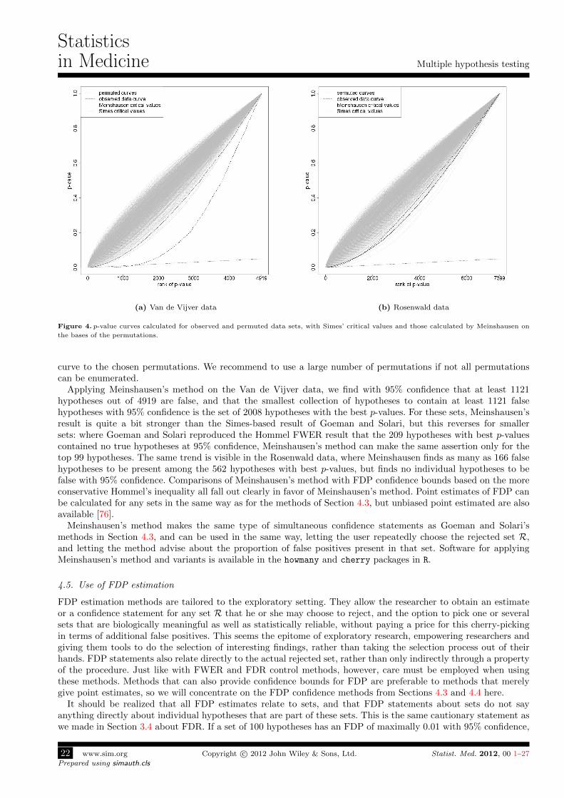
Statisticsin Medicine Multiple hypothesis testing
(a) Van de Vijver data (b) Rosenwald data
Figure 4. p-value curves calculated for observed and permuted data sets, with Simes’ critical values and those calculated by Meinshausen on
the bases of the permutations.
curve to the chosen permutations. We recommend to use a large number of permutations if not all permutationscan be enumerated.
Applying Meinshausen’s method on the Van de Vijver data, we find with 95% confidence that at least 1121hypotheses out of 4919 are false, and that the smallest collection of hypotheses to contain at least 1121 falsehypotheses with 95% confidence is the set of 2008 hypotheses with the best p-values. For these sets, Meinshausen’sresult is quite a bit stronger than the Simes-based result of Goeman and Solari, but this reverses for smallersets: where Goeman and Solari reproduced the Hommel FWER result that the 209 hypotheses with best p-valuescontained no true hypotheses at 95% confidence, Meinshausen’s method can make the same assertion only for thetop 99 hypotheses. The same trend is visible in the Rosenwald data, where Meinshausen finds as many as 166 falsehypotheses to be present among the 562 hypotheses with best p-values, but finds no individual hypotheses to befalse with 95% confidence. Comparisons of Meinshausen’s method with FDP confidence bounds based on the moreconservative Hommel’s inequality all fall out clearly in favor of Meinshausen’s method. Point estimates of FDP canbe calculated for any sets in the same way as for the methods of Section 4.3, but unbiased point estimated are alsoavailable [76].
Meinshausen’s method makes the same type of simultaneous confidence statements as Goeman and Solari’smethods in Section 4.3, and can be used in the same way, letting the user repeatedly choose the rejected set R,and letting the method advise about the proportion of false positives present in that set. Software for applyingMeinshausen’s method and variants is available in the howmany and cherry packages in R.
4.5. Use of FDP estimation
FDP estimation methods are tailored to the exploratory setting. They allow the researcher to obtain an estimateor a confidence statement for any set R that he or she may choose to reject, and the option to pick one or severalsets that are biologically meaningful as well as statistically reliable, without paying a price for this cherry-pickingin terms of additional false positives. This seems the epitome of exploratory research, empowering researchers andgiving them tools to do the selection of interesting findings, rather than taking the selection process out of theirhands. FDP statements also relate directly to the actual rejected set, rather than only indirectly through a propertyof the procedure. Just like with FWER and FDR control methods, however, care must be employed when usingthese methods. Methods that can also provide confidence bounds for FDP are preferable to methods that merelygive point estimates, so we will concentrate on the FDP confidence methods from Sections 4.3 and 4.4 here.
It should be realized that all FDP estimates relate to sets, and that FDP statements about sets do not sayanything directly about individual hypotheses that are part of these sets. This is the same cautionary statement aswe made in Section 3.4 about FDR. If a set of 100 hypotheses has an FDP of maximally 0.01 with 95% confidence,
22 www.sim.org Copyright c© 2012 John Wiley & Sons, Ltd. Statist. Med. 2012, 00 1–27
Prepared using simauth.cls
Multiple hypothesis testing
Statisticsin Medicine
then each individual hypothesis among these 100 may or may not be a likely candidate for a false positive. Unlikewith FDR, however, this problem is alleviated by the fact that FDP confidence methods do simultaneously provideconfidence bounds for all subsets of the set R. These simultaneous subset statements at least partially solve thecheating problem (Section 3.4), because a valid confidence statement is always available for the set of hypothesesof real interest. The methods also allow statements to be made for individual hypotheses, by obtaining confidencestatements for subsets of R of size 1. To completely avoid problems of overinterpretation of FDP statements aboutsets, however, ideally all 2m − 1 simultaneous confidence statements should be reported. This is impossible, ofcourse, and the sets for which the confidence bounds are calculated and reported should be chosen carefully.
Because of the identity between the underlying methods, FDP confidence statements actually come for free withthe use of Hochberg’s and Hommel’s methods. Using Hommel’s FWER control and FDP confidence together, theFWER-controlled rejections are augmented by weaker statements for the set of hypotheses that just did not makethe FWER threshold, claiming that at least a proportion of these hypotheses is false. These may be forwarded tofurther validation experiments if the FDP confidence bound for such a set is promising enough.
FDP confidence methods are most fruitfully used in exploratory settings if much freedom is desired in pickingand choosing the set of rejected hypotheses of interest, or if more specific and more confident FDP statements arerequired than those provided by FDR control.
5. Reducing the number of tests
So far, we have assumed that the collection of hypotheses to be tested was fixed a priori. In practical testingproblems this does not have to be the case. Even if tens of thousands of probes or more have been measured ona genomic chip, this does not mean that all of these data as such have to be fed into the testing procedure. Infact, there are large gains to be had by either selecting a more limited number of hypotheses to be tested, or byaggregating hypotheses in order to test them jointly. In practice these gains can be much greater than the gainobtained by changing from one multiple testing procedure to another more powerful one. We discuss selection andaggregation in turn.
5.1. Selection
The more hypotheses, the bigger the multiple testing problem. This holds immediately for FWER control methodsand FDP confidence methods, which are always more powerful if fewer hypotheses are being tested. By this wemean that discarding some hypotheses before performing the testing procedure always leads to more rejections ortighter confidence bounds among the remaining hypotheses than discarding the same hypotheses after performingthe same procedure. The same is not always true for FDR-controlling methods, as we have seen in Section 3.4, butalso for those methods removing hypotheses prior to testing tends to result in more power, especially if the discardedhypotheses are predominantly either true hypotheses or false hypotheses for which the test has low power. Anyway,with FDR control, any discarding needs to be done before testing, since discarding after testing risks loss of FDRcontrol. Of course, discarding of hypotheses brings the risk of discarding hypotheses that would have been highlysignificant if not discarded. Discarded hypotheses should therefore be chosen either because they are uninteresting,or because they have low power.
Uninteresting hypotheses are hypotheses whose rejection the researcher would not follow up on even if theycame out with the smallest p-value. Surprisingly many of such uninteresting hypotheses are tested in genomicsexperiments. Many researchers, for example, are only interested in annotated probes, i.e. probes for which thename of the associated gene is known. Tests of non-annotated probes typically also have low power, because theyare often low-expressed, and therefore seldom show up on the top of the list of significant genes. If they do, theyare often either ignored or thrown out after the analysis. Non-annotated probes make up over 35% of the probes inthe Van de Vijver data. Using Holm’s method as an example, out of 206 hypotheses rejected without selection, 158are annotated. Removing non-annotated probes before testing, the number of annotated probes rejected increasesto 176.
Discarding hypotheses with low power before testing can also benefit the overall power of the multiple testingprocedure. If there are hypotheses that are very unlikely to give a small enough p-value to be rejected, the onlyeffect of including them is to worsen the critical values of more promising hypotheses. Deciding which hypotheseshave insufficient power is often done on the basis of the data, but only certain aspects of the data may be usedwithout compromising type I error control. As a rule of thumb the selection criterion must be independent of thep-values, but precisely what can or should be used depends on the specifics of model and data [77, 78, 79, 80]. Ingene expression data, a viable and powerful selection is to discard probes with low mean or low variance under the
Statist. Med. 2012, 00 1–27 Copyright c© 2012 John Wiley & Sons, Ltd. www.sim.org 23Prepared using simauth.cls
Statisticsin Medicine Multiple hypothesis testing
null hypothesis, since both of these are indicators of low biological variation in gene expression. In the Rosenwalddata, removing the 50% probes with low mean expression, we get 6 rejections with Holm’s method rather than 4.Compared to a priori discarding of uninteresting probes, selection on the basis of presumed power is more risky:good results may be discarded with the bad. We see an example of this in the Rosenwald data if we select on highvariance of expression instead of high mean: this leaves us with only 3 rejected probes. Researchers concerned aboutthis risk may want to consider weighted multiple testing as an alternative to selection, down-weighting rather thandiscarding hypotheses with low power [77, 78].
It is interesting to remark that the two selection criteria of interestingness and power often at least partiallycoincide. In the examples above, on the one hand non-annotated probes are often low expressed, and thereforetypically have low power. On the other hand, probes with low mean or variance of expression are unlikely to havea large magnitude of differential expression, even if they would have a very low p-value. Such a significant probewith a small effect size is less trustworthy and is often found less interesting than one with a large effect size.
5.2. Aggregation
A different way of reducing the size of the testing problem is to aggregate the data to a lower resolution. Forexample, rather than testing every probe, aggregated tests can be performed at the gene level or at the level of achromosomal region. Such aggregation is especially beneficial if the aggregated level is the level of primary biologicalinterest. Not only does aggregation reduce the size of the testing problem, aggregated tests also tend to be morepowerful than non-aggregated ones.
The choice of an aggregated test should be determined by the type of data, the level of aggregation, and domainknowledge. In gene expression data, for example, we would expect different probes of the same gene to showapproximately the same amount and direction of differential expression. With this in mind, a suitable aggregatetest at the gene level would just calculate the gene’s expression as an average of each probe’s expression, and use thisas a basis for testing. When aggregating to higher levels than the gene, or when the possibility of differential splicingleads us to expect highly heterogeneous differential expression of probes, then more sophisticated aggregated testsmay be preferable [38, 39]. In all cases, the formal null hypothesis of an aggregated test is that the hypotheses of allof the probes that have been aggregated are true. In the Van de Vijver data the 3179 annotated probes represent3043 genes, so there is not much to be aggregated. Still, taking Holm’s method as an example again, we see that the176 annotated probes rejected in Section 5.1 correspond to 170 genes. Aggregating to the gene level before testing,using simple averaging of probes, improves this to 173 rejected genes.
If not only the aggregated level is of interest, but also lower or higher levels of resolution, then it is possible touse hierarchical multiple testing methods that test more than one level of resolution simultaneously. Such methodsstart testing at the most aggregated level, continuing to a more detailed resolution only at those locations forwhich significant results have been found. Hierarchical methods are available for both FDR and FWER control[81, 82, 83, 84]. This type of methods can also be used in the situation that multiple hypotheses are tested aboutthe each probe, by first rejecting the overal null hypothesis for each probe that all these hypotheses are true, beforegoing down to the detailed tests of the individual hypotheses for that probe.
6. Discussion and conclusion
A typical genomics experiment involves many thousands of hypothesis tests. It is unavoidable, therefore that boththe researcher him- or herself, and the reader of the resulting publication, only sees a very small selection of theresults of these tests. Human intuition is not capable of quantifying the effect of this selection: formal methods areneeded to correct for it. This is what multiple testing methods are for.
From this perspective, there can be no reason not to correct for multiple testing in a genomics experiment. Evenif a user is not prepared to let the results of a multiple testing method dictate his or her actions, the results of amultiple testing method carry information about the effect of selection on the reliability of any conclusions drawn.The least such a user can do is to estimate the number of false positives in the selected set, as the methods ofSection 4 allow to do.
Multiple testing methods traditionally only concentrate on the effect of selection on p-values and on rejection ofhypotheses. Selection, however, also biases effect size estimates. The estimated fold change of differential expressionof the probe with highest expression is very likely to be overestimated, and is therefore subject to a regression to themean effect upon replication of the experiment. This is the famous winner’s curse, which has been much discussedin the context of genomewide association experiments, where it shows up in the odds ratios of top SNPs [85].
24 www.sim.org Copyright c© 2012 John Wiley & Sons, Ltd. Statist. Med. 2012, 00 1–27
Prepared using simauth.cls

Multiple hypothesis testing
Statisticsin Medicine
One other aspect that is universally ignored by multiple testing methods is the haphazard trying of differentmodels and analysis techniques that is typical of actual data analysis. Models are fitted with and without certaincovariates; several tests may be tried. In the end, it is more likely that a model with many significant results isselected for the final analysis than one with few. Such model tuning may severely bias the p-values downward, andincrease the likelihood that type I errors appear. Since this process is highly unstructured, it is impossible to formallycorrect for it. The resulting bias can be prevented by writing a complete analysis plan before data collection, andadhering strictly to it, but this is something few researchers in genomics experiments will be prepared to do. It canalso be prevented by good and independent validation experiments.
It cannot be stressed enough that if any multiple testing is applied anywhere, it must be in the independentvalidation experiments. The results of validation experiments must be able to hold their own, individually, andwithout further evidence to back them up. Familywise error control is the norm here. If a genomics experiment isnot followed up by independent biological validation, it must be very strict in its multiple testing correction, sincethe experiment essentially doubles as its own validation.
When choosing a multiple testing correction method, two important questions need to be asked. First, whatassumptions can be made about the joint distribution of the p-values observed in the experiment? Second, whattype of multiple testing method is needed? We will finish this tutorial by briefly reiterating some of the considerationsthat can play a role when answering both these questions.
Regarding the assumptions on the p-value distribution, it is important to realize that p-values in genomicsexperiments are never independent, so that any methods that assume such independence should be approachedwith great care, if at all. Three more realistic options have been most often considered in the literature: methodsbased on either permutations, on Simes’ inequality, or assumption-free methods. Permutation-based methods havemost to be said for them, as they adapt powerfully to the unknown joint distribution of the p-values and do not relyon the validity of the asymptotics of the raw p-values. Permutation methods are not completely assumption-free,however, and they are not available for all experimental designs. Computation time can also be a limiting factorwhen using them. Simes-based methods are an alternative, which can be assumed to be valid for the ubiquitoussituation of two-sided test statistics that are at least asymptotically normal. Assumption-free methods can alwaysbe used, but generally sacrifice a lot of power relative to the other two types of methods, and should be consideredonly in situations that permutations and Simes-based methods are both excluded.
The type of multiple testing correction to be used depends crucially on the way the results are going to beused or reported. If individual rejected hypotheses are of interest, and if author or reader of the results is likely totake subsets of the collection of rejected hypotheses out of the context of the complete rejected set, then FWERcontrolling methods are advisable. If, on the other hand, the collection of rejected results as a whole is of interest,either because this entire collection is to be forwarded to a validation experiment, or because the overview is ofinterest, rather than the detailed results, then the FDP of this collection should be the focus, and FDR or FDP-type methods are preferable. FDP confidence methods are between FDR and FWER methods in many respects,sacrificing some of the power of FDR methods, but gaining more protection against the variability of FDP aroundFDR, and gaining the ability to make simultaneous statements about interesting subsets and supersets of the chosenresults. These methods are especially useful if the hypotheses with top p-values are not necessarily all automaticallyof interest, but greater flexibility in decision-making is desired.
References
1. Dudoit S, Shaffer J, Boldrick J. Multiple hypothesis testing in microarray experiments. Statistical Science 2003; 18(1):71–103.
2. Benjamini Y. Simultaneous and selective inference: current successes and future challenges. Biometrical Journal 2010; 52(6):708–
721.3. Farcomeni A. A review of modern multiple hypothesis testing, with particular attention to the false discovery proportion. Statistical
Methods in Medical Research 2008; 17(4):347–388.4. Roquain E. Type I error rate control for testing many hypotheses: a survey with proofs. Journal de la Societe Francaise de
Statistique 2011; 153(2):3–38.
5. Dudoit S, van der Laan M. Multiple testing procedures with applications to genomics. Springer Verlag, 2008.6. Cox D. A remark on multiple comparison methods. Technometrics 1965; 7(2):223–224.
7. Benjamini Y, Yekutieli D. False discovery rate-adjusted multiple confidence intervals for selected parameters. Journal of the
American Statistical Association 2005; 100(469):71–81.8. Ioannidis J. Why most published research findings are false. PLoS medicine 2005; 2(8):e124.
9. Rothstein H, Sutton A, Borenstein M. Publication Bias in Meta-Analysis. Wiley Online Library, 2005.
10. Bender R, Lange S. Adjusting for multiple testing–when and how? Journal of Clinical Epidemiology 2001; 54(4):343–349.11. Goeman J, Solari A. Multiple testing for exploratory research. Statistical Science 2012; 26(4):584–597.
Statist. Med. 2012, 00 1–27 Copyright c© 2012 John Wiley & Sons, Ltd. www.sim.org 25Prepared using simauth.cls

Statisticsin Medicine Multiple hypothesis testing
12. Benjamini Y, Hochberg Y. Controlling the false discovery rate: a practical and powerful approach to multiple testing. Journal ofthe Royal Statistical Society. Series B (Methodological) 1995; 57(1):289–300.
13. Storey J. The positive false discovery rate: A Bayesian interpretation and the q-value. The Annals of Statistics 2003; 31(6):2013–
2035.14. Finner H, Roters M. On the false discovery rate and expected type I errors. Biometrical Journal 2001; 43(8):985–1005.
15. Guo W, Bhaskara Rao M. On control of the false discovery rate under no assumption of dependency. Journal of Statistical Planningand Inference 2008; 138(10):3176–3188.
16. Simes R. An improved Bonferroni procedure for multiple tests of significance. Biometrika 1986; 73(3):751–754.
17. Sarkar S. Some probability inequalities for ordered mtp2 random variables: a proof of the simes conjecture. The Annals of Statistics1998; 26(2):494–504.
18. Sarkar S. Two-stage stepup procedures controlling FDR. Journal of Statistical Planning and Inference 2008; 138(4):1072–1084.
19. Benjamini Y, Yekutieli D. The control of the false discovery rate in multiple testing under dependency. Annals of statistics 2001;29(4):1165–1188.
20. Rødland E. Simes’ procedure is ‘valid on average’. Biometrika 2006; 93(3):742–746.
21. Sarkar S. Fdr-controlling stepwise procedures and their false negatives rates. Journal of Statistical Planning and Inference 2004;125(1):119–137.
22. Reiner-Benaim A. Fdr control by the bh procedure for two-sided correlated tests with implications to gene expression data analysis.
Biometrical Journal 2007; 49(1):107–126.23. Kim K, Van De Wiel M. Effects of dependence in high-dimensional multiple testing problems. BMC Bioinformatics 2008; 9(1):114.
24. Yekutieli D. Comments on: Control of the false discovery rate under dependence using the bootstrap and subsampling. Test 2008;17(3):458–460.
25. Finner H, Dickhaus T, Roters M. On the false discovery rate and an asymptotically optimal rejection curve. The Annals of Statistics
2009; 37(2):596–618.26. Good P. Permutation tests. Wiley Online Library, 2000.
27. Pesarin F. Multivariate permutation tests: with applications in biostatistics. Wiley Chichester, 2001.
28. Huang Y, Xu H, Calian V, Hsu J. To permute or not to permute. Bioinformatics 2006; 22(18):2244–2248.29. Goeman J, Solari A. The sequential rejection principle of familywise error control. The Annals of Statistics 2010; 38(6):3782–3810.
30. Risch N, Merikangas K. The future of genetic studies of complex human diseases. Science 1996; 273(5281):1516–1517.
31. Hoggart C, Clark T, De Iorio M, Whittaker J, Balding D. Genome-wide significance for dense SNP and resequencing data. GeneticEpidemiology 2008; 32(2):179–185.
32. Van De Vijver M, He Y, Van’t Veer L, Dai H, Hart A, Voskuil D, Schreiber G, Peterse J, Roberts C, Marton M, et al.. A
gene-expression signature as a predictor of survival in breast cancer. New England Journal of Medicine 2002; 347(25):1999–2009.33. Rosenwald A, Wright G, Chan W, Connors J, Campo E, Fisher R, Gascoyne R, Muller-Hermelink H, Smeland E, Giltnane J, et al..
The use of molecular profiling to predict survival after chemotherapy for diffuse large-B-cell lymphoma. New England Journal ofMedicine 2002; 346(25):1937–1947.
34. Blanchard G, Dickhaus T, Hack N, Konietschke F, Rohmeyer K, Rosenblatt J, Scheer M, Werft W. µtoss—multiple hypothesis
testing in an open software system. Journal of Machine Learning Research: Workshop and Conference Proceedings, vol. 11, 2010.35. Perneger T. What’s wrong with Bonferroni adjustments. British Medical Journal 1998; 316(7139):1236–1238.
36. Sidak Z. Rectangular confidence regions for the means of multivariate normal distributions. Journal of the American Statistical
Association 1967; 62(318):626–633.37. Rothman K. No adjustments are needed for multiple comparisons. Epidemiology 1990; 1(1):43–46.
38. Goeman J, Van De Geer S, De Kort F, Van Houwelingen H. A global test for groups of genes: testing association with a clinical
outcome. Bioinformatics 2004; 20(1):93–99.39. Hummel M, Meister R, Mansmann U. Globalancova: exploration and assessment of gene group effects. Bioinformatics 2008;
24(1):78–85.
40. Holm S. A simple sequentially rejective multiple test procedure. Scandinavian Journal of Statistics 1979; 6(2):65–70.41. Hochberg Y. A sharper bonferroni procedure for multiple tests of significance. Biometrika 1988; 75(4):800–802.
42. Marcus R, Peritz E, Gabriel K. On closed testing procedures with special reference to ordered analysis of variance. Biometrika
1976; 63(3):655–660.43. Hommel G. A stagewise rejective multiple test procedure based on a modified Bonferroni test. Biometrika 1988; 75(2):383–386.
44. Hommel G. A comparison of two modified Bonferroni procedures. Biometrika 1989; 76(3):624–625.45. Westfall P, Young S. Resampling-based multiple testing: Examples and methods for p-value adjustment, vol. 279. Wiley-Interscience,
1993.
46. Meinshausen N, Maathuis M, Buhlmann P. Asymptotic optimality of the Westfall–Young permutation procedure for multipletesting under dependence. The Annals of Statistics 2012; 39(6):3369–3391.
47. Ge Y, Dudoit S, Speed T. Resampling-based multiple testing for microarray data analysis. Test 2003; 12(1):1–77.
48. Phipson B, Smyth G. Permutation p-values should never be zero: calculating exact p-values when permutations are randomlydrawn. Statistical Applications in Genetics and Molecular Biology 2010; 9(1):39.
49. Benjamini Y, Hochberg Y. On the adaptive control of the false discovery rate in multiple testing with independent statistics.
Journal of Educational and Behavioral Statistics 2000; 25(1):60–83.50. Benjamini Y, Krieger A, Yekutieli D. Adaptive linear step-up procedures that control the false discovery rate. Biometrika 2006;
93(3):491–507.
51. Blanchard G, Roquain E. Adaptive false discovery rate control under independence and dependence. The Journal of MachineLearning Research 2009; 10:2837–2871.
52. Sarkar S, Guo W, Finner H. On adaptive procedures controlling the familywise error rate. Journal of Statistical Planning andInference 2012; 142(1):65–78.
53. Blanchard G, Roquain E. Two simple sufficient conditions for FDR control. Electronic Journal of Statistics 2008; 2:963–992.
26 www.sim.org Copyright c© 2012 John Wiley & Sons, Ltd. Statist. Med. 2012, 00 1–27
Prepared using simauth.cls

Multiple hypothesis testing
Statisticsin Medicine
54. Yekutieli D, Benjamini Y. Resampling-based false discovery rate controlling multiple test procedures for correlated test statistics.Journal of Statistical Planning and Inference 1999; 82(1-2):171–196.
55. Romano J, Shaikh A, Wolf M. Control of the false discovery rate under dependence using the bootstrap and subsampling. Test
2008; 17(3):417–442.56. Troendle J. Stepwise normal theory multiple test procedures controlling the false discovery rate. Journal of Statistical Planning
and Inference 2000; 84(1-2):139–158.57. Ge Y, Sealfon S, Speed T. Some step-down procedures controlling the false discovery rate under dependence. Statistica Sinica
2008; 18(3):881–904.
58. Korn E, Troendle J, McShane L, Simon R. Controlling the number of false discoveries: application to high-dimensional genomicdata. Journal of Statistical Planning and Inference 2004; 124(2):379–398.
59. Finner H, Dickhaus T, Roters M. Dependency and false discovery rate: asymptotics. The Annals of Statistics 2007; :1432–1455.
60. Troendle J. Comments on: Control of the false discovery rate under dependence using the bootstrap and subsampling. Test 2008;17(3):456–457.
61. Goeman J, Mansmann U. Multiple testing on the directed acyclic graph of gene ontology. Bioinformatics 2008; 24(4):537–544.
62. Posch M, Zehetmayer S, Bauer P. Hunting for significance with the false discovery rate. Journal of the American StatisticalAssociation 2009; 104(486):832–840.
63. Storey J. A direct approach to false discovery rates. Journal of the Royal Statistical Society: Series B (Statistical Methodology)
2002; 64(3):479–498.64. Storey J, Taylor J, Siegmund D. Strong control, conservative point estimation and simultaneous conservative consistency of false
discovery rates: a unified approach. Journal of the Royal Statistical Society: Series B (Statistical Methodology) 2004; 66(1):187–205.65. Schwartzman A, Lin X. The effect of correlation in false discovery rate estimation. Biometrika 2011; 98(1):199–214.
66. Pounds S, Cheng C. Improving false discovery rate estimation. Bioinformatics 2004; 20(11):1737–1745.
67. Owen A. Variance of the number of false discoveries. Journal of the Royal Statistical Society: Series B (Statistical Methodology)2005; 67(3):411–426.
68. Qiu X, Yakovlev A. Some comments on instability of false discovery rate estimation. Journal of Bioinformatics and Computational
Biology 2006; 4(5):1057–1068.69. Efron B, Tibshirani R, Storey J, Tusher V. Empirical bayes analysis of a microarray experiment. Journal of the American Statistical
Association 2001; 96(456):1151–1160.
70. Qiu X, Klebanov L, Yakovlev A. Correlation between gene expression levels and limitations of the empirical bayes methodology inmicroarray data analysis. Statistical Applications in Genetics and Molecular Biology 2005; 4(1):34.
71. Pawitan Y, Calza S, Ploner A. Estimation of false discovery proportion under general dependence. Bioinformatics 2006;
22(24):3025–3031.72. Efron B. Correlation and large-scale simultaneous significance testing. Journal of the American Statistical Association 2007;
102(477):93–103.73. Efron B. Correlated z-values and the accuracy of large-scale statistical estimates. Journal of the American Statistical Association
2010; 105(491):1042–1055.
74. Goeman J, Solari A. Rejoinder. Statistical Science 2011; 26(4):608–612.75. Meinshausen N. False discovery control for multiple tests of association under general dependence. Scandinavian Journal of
Statistics 2006; 33(2):227–237.
76. Lee W, Gusnanto A, Salim A, Magnusson P, Sim X, Tai E, Pawitan Y. Estimating the number of true discoveries in genome-wideassociation studies. Statistics in Medicine 2011; 31(11–12):1177–1189.
77. Hommel G, Kropf S. Tests for differentiation in gene expression using a data-driven order or weights for hypotheses. Biometrical
journal 2005; 47(4):554–562.78. Finos L, Salmaso L. Fdr-and fwe-controlling methods using data-driven weights. Journal of Statistical Planning and Inference
2007; 137(12):3859–3870.
79. Hackstadt A, Hess A. Filtering for increased power for microarray data analysis. BMC Bioinformatics 2009; 10(1):11.80. van Iterson M, Boer J, Menezes R. Filtering, FDR and power. BMC Bioinformatics 2010; 11(1):450.
81. Meinshausen N. Hierarchical testing of variable importance. Biometrika 2008; 95(2):265–278.82. Yekutieli D. Hierarchical false discovery rate-controlling methodology. Journal of the American Statistical Association 2008;
103(481):309–316.
83. Benjamini Y, Bogomolov M. Adjusting for selection bias in testing multiple families of hypotheses. Arxiv preprint arXiv:1106.36702011; .
84. Goeman J, Finos L. The inheritance procedure: multiple testing of tree-structured hypotheses. Statistical Applications in Geneticsand Molecular Biology 2012; 11(1):1–18.
85. Zhong H, Prentice R. Correcting ‘winner’s curse’ in odds ratios from genomewide association findings for major complex human
diseases. Genetic Epidemiology 2010; 34(1):78–91.
Statist. Med. 2012, 00 1–27 Copyright c© 2012 John Wiley & Sons, Ltd. www.sim.org 27Prepared using simauth.cls