ZIVE Application Note8: potentiodynamic PEIS Test for corrosion 

Potentiodynamic PEIS Test for Corrosion Application 

Purpose 

This test is to demonstrate Corrosion EIS test.  This will measure PEIS by changing bias potential with staircase wave form. This complex procedure can be tested with frequency scanning potentiodynamic PEIS in technique menu.  

This demonstration’s test condition is; 

Start potential: ‐700mVvs Eoc 

Final potential: 600mV vs Eoc 

Voltage step: 20mV 

EIS measurement at each potential step 

Initial frequency: 1MHz 

Final frequency: 0.1Hz 

Amplitude: 10mV 

Points per decade: 10 

 Preparation 

ZIVE SP/MP electrochemical workstation 

Corrosion cell (universal cell holder) 

Coin Cell holder 

Cell Connection 

+ electrode(Green lead & Blue lead) ‐ electrode(White lead & Red lead) 

 

 

 

 

Procedure 

1. Turn the Power switch on the ZIVE SP/MP electrochemical workstation 2. Open the SM software by clicking the SM icon. The following progress box will appear, and will show the progress of checking instrument 

configuration and communication between ZIVE SP/MP electrochemical workstation and PC. 

  If the link is successfully connected, Click “OK” button on the box then the progress box will automatically disappear and SM software will appear. If the link failed, The following progress box will display then click the “Retry” button.  

 If the link failed again after clicking “Retry” button, you need to check USB cable connection. 

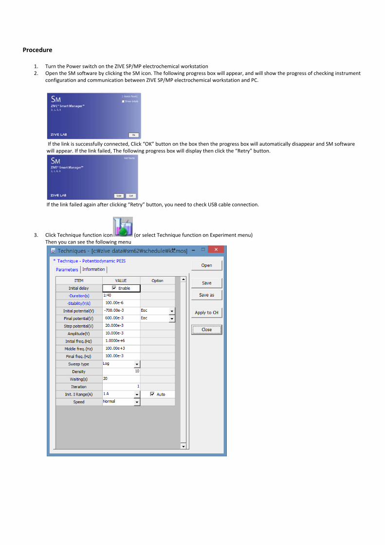
3. Click Technique function icon  (or select Technique function on Experiment menu) Then you can see the following menu 

   

4. Select Frequency scanning potentiodynamic PEIS at left technique selection region. The parameter editing region is located at right.  Input figure for parameter setting as the follows.. 

 5. Click “Save” button to save the technique file which contains the above parameter and setting file name. 6. You can assign this technique file to channel(s) which you want by click “APPLY” button or select schedule file using file selection on 

“Single channel control/monitor” or “multi channel control/monitor” If you click “apply” button on technique menu, You can see the following channel selection menu. 

 Select channel and click OK then this technique file will be assigned on the channel. Click “Close” button or minimize technique window. 

7. If you want control ZIVE SP/MP electrochemical workstation using “Single channel control/monitor”, you can see following windows. 

 

To start experiment, click Start button  

If you want control ZIVE SP/MP multichannel, you can see the following window 

 

To start experiment for specific channel, click Start button  on the channel. If you want to start experiment for multiple channel, 

click on Group column which you want to start and click Start button  at bottom side. 

8. After click start button, you can see the following box. 

 

The data file name is automatically determined as default value but if you want to change data file folder then click    icon 

 

You can make new folder which you want to save. 

If you want use your file name, input your file name on “File name” 

If you did not make file name manually, new data folder which named as sequence file name or technique file name under 

data folder and it’s subfolder will be created with name as date. The data file will be saved in this folder. The data file name 

will be determined automatically as string with sequence file name or technique file name and hour and minute and second, 

finally channel number will be added. 

example) If you used sequence file for test  and its file name is testabc.zsc and channel number is 1 and test date is  2000 year 

January 1st  time is 15:30: 1 then the data file will be saved as 

C:\Zive data\sm\data\testabc.zsc\2000010115\3001_01.sdo (If data file have DC data only) 

Or 

C:\Zive data\sm\data\testabc.zsc\2000010115\3001_01.sde (If data file have DC data and EIS data) 

Or 

C:\Zive data\sm\data\testabc.zsc\2000010115\3001_01.seo (If data file have EIS data only) 

 

e.g.) schedule file name with extension\yearmonthdayhour\minutesecond_channel number 

If you input file name as “tommy” then  

C:\Zive data\sm\data\testabc.zsc\2000010115\tommy3001_01.sdo (sde,seo) 

① Start Step: If your sequence file has several steps, you can select starting step. 

② Start file: If batch file is loaded, select file number 

③ Current polarity: If you want reverse polarity for measured current, check on this box. 

④ Active area: For calculation of current density 

⑤ Capacity: For C‐rate value calculation 

⑥ Weight: For specific capacity calculation 

⑦ Tester: Operator name 

⑧ Memo: Text information for test (For line change, use CTRL+ENTER) 

No Save file: If you click this check box, the data will NOT be saved.  

  

If you are ready to test, click OK button then experiment will be started. 

 

You can see real time plot as the following. 

 

Real time EIS graph shows sub window at right upper side. This window display sine wave or E vs. I graph to check data quality. Default 

display is sine wave. 

 This shows two sine wave graphs. One is for current (green line) and the other is for voltage (Yellow line). 

If you switch this graph to I vs E, double click on the graph then graph format will be changed. 

 

9. You can display graphic by clicking button   on tool bar Click “Open data file” icon and select data file which you run the experiment. 

 

You can select Bode plot by clicking  icon or Nyquist plot by clicking   icon. 

 

SM can split each EIS graph by selecting “step” in “division”. 

You can split data by file, cycle or step. Splitted data set’s color was changed and graph line will be broken 

ZMAN will split each EIS data automatically if you insert “cycle” mark. 

. 

For user defined graphic, you can select X axis and Max 4 Y axis parameter as you wanted. 

 

Data Analysis 

1. Open “ZMAN” by clicking ZMAN icon. ZMAN program is located c:\program files\zivelab\zman2.2 folder. 2. You can see the following window. 

 3.  Click “Yes” then multiple EIS data will be splitted automatically. 

 

If you do not want to use all EIS data set, Click “No” then you can see select box. 

 You can select one EIS data for analysis. 

 

 

4. You can see Impedance,Admittance,Modulus,Dielectric Constant by selecting as the following a) Select data set 

 

b) Seelect Impedance,Z in polar,Admittance,Y in Polar, Modulus, M in polar, Dielectric Constant, E in polar. (in polar = in Polar Coordinate) 

 

5. Click 2D nyquist plot 

 You can show plot as 1:1 scale  for nyquist plot by clicking right button of mouse and select “matching scale”  

 Matching scale is X axis scale and Y axis scale on graph is same. You can check each data value by selecting “cursor” with clicking right button of mouse . 

 

You can move the point by dragging the mouse after check cursor icon . 

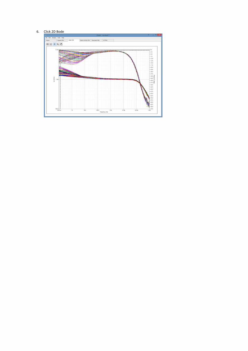
6. Click 2D Bode  

 

Anaysis 

A. Two circles Nyquist  spectra (model fitting using circular fit: Manual Modeling) 

1. You can select fitting method by your purpose Circular fit or Modeling & fitting 

 

a. Circular fit a. Select circular fit on Analysis and Move left(biolet) & right cursor(green line) into 2st circle region 

 

b. click Initial guessing icon  

c. Click fitting icon 1time or 10 time fitting   

 

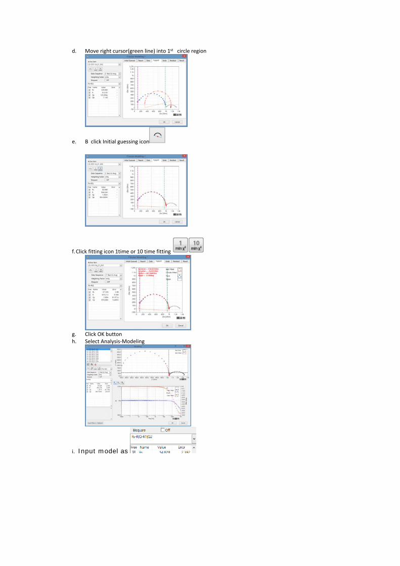
d. Move right cursor(green line) into 1st   circle region 

 

e. B  click Initial guessing icon  

f. Click fitting icon 1time or 10 time fitting   

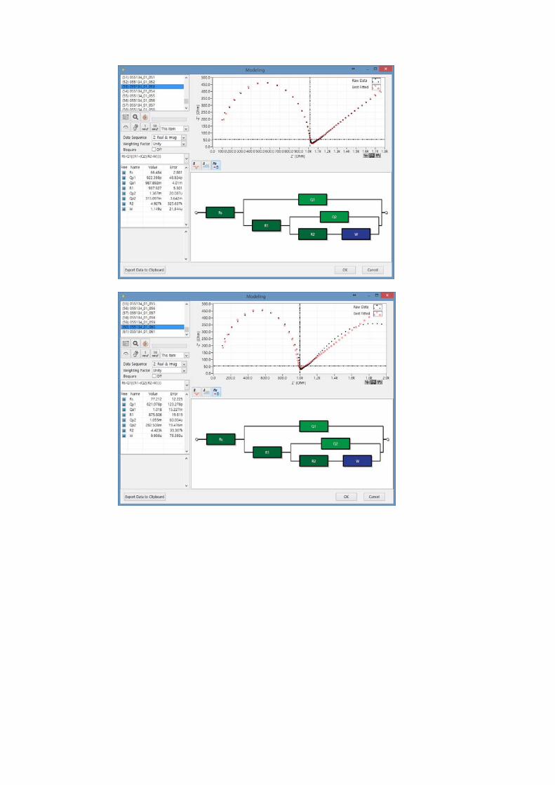
 g. Click OK button h. Select Analysis‐Modeling 

 

i. Input model as  

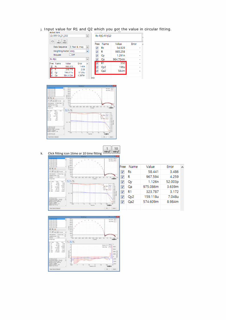
j. Input value for R1 and Q2 which you got the value in circular fitting.

=>  

k. Click fitting icon 1time or 10 time fitting   

 

 

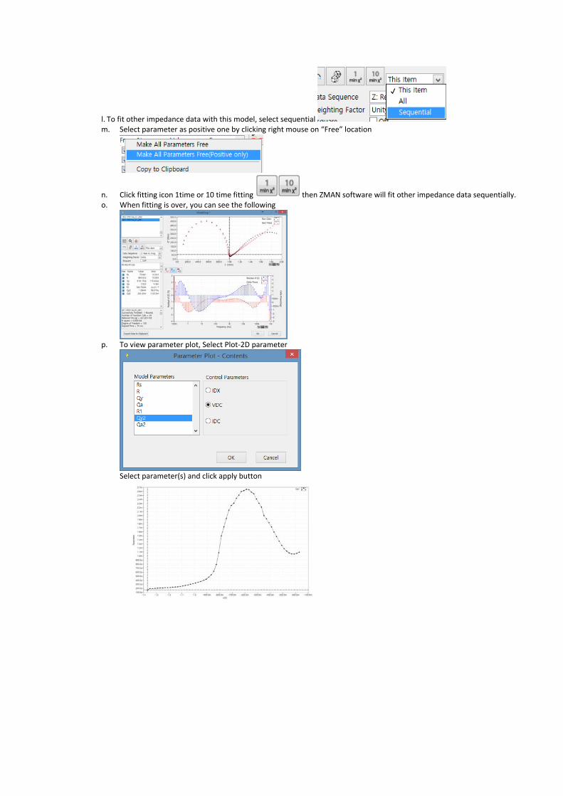
l. To fit other impedance data with this model, select sequential   m. Select parameter as positive one by clicking right mouse on “Free” location 

 

n. Click fitting icon 1time or 10 time fitting   then ZMAN software will fit other impedance data sequentially. o. When fitting is over, you can see the following 

 p. To view parameter plot, Select Plot‐2D parameter 

 Select parameter(s) and click apply button 

 

 

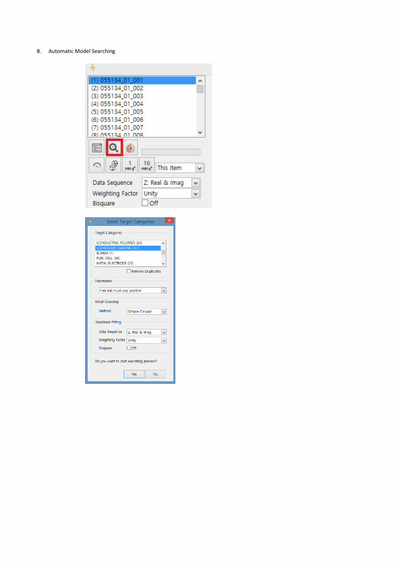
B. Automatic Model Searching 

 

 

 

 

a. You can see Nyquist or Bode data with fitted data 

   b. 3D graph 

 

Nyquist plot vs potential 

 

Bode Impedance vs potential 

 

Bode phase vs potential 

Tafel plot during DC potential scanning

 

 

 

 

 

 

 

Copyright○c 2011 ZiveLab