Post-Buckling Behaviour Of Metallic Skin-Stringer

POST-BUCKLING BEHAVIOUR OF METALLIC SKIN-STRINGER

ASSEMBLIES AND BUCKLING OF COMPOSITE FLAT PANELS

A THESIS SUBMITTED TO

THE GRADUATE SCHOOL OF NATURAL AND APPLIED SCIENCES

OF

MIDDLE EAST TECHNICAL UNIVERSITY

BY

ENES AYDIN

IN PARTIAL FULFILLMENT OF THE REQUIREMENTS

FOR

THE DEGREE OF MASTER OF SCIENCE

IN

AEROSPACE ENGINEERING

MARCH 2018

Approval of the thesis:



Submitted by ENES AYDIN in partial fulfillment of the requirements for the degree

of Master of Science in The Department of Aerospace Engineering, Middle East

Technical University by,

Prof. Dr. Halil Kalıpçılar

Dean, Graduate School of Natural and Applied Sciences

Prof. Dr. Ozan Tekinalp

Head of Department, Aerospace Engineering

Prof. Dr. Altan Kayran

Supervisor, Aerospace Engineering Department, METU

Examining Committee Members:

Assoc. Prof. Dr. Demirkan Çöker

Aerospace Engineering Department, METU

Prof. Dr. Altan Kayran


Assoc. Prof. Dr. Ercan Gürses


Assoc. Prof. Dr. Melin Şahin

Aerospace Engineering Department,

METU

Asst. Prof. Dr. Barış Sabuncuoğlu

Mechanical Engineering, Hacettepe University

Date:

iv

I hereby declare that all information in this document has been obtained and

presented in accordance with academic rules and ethical conduct. I also declare

that, as required by these rules and conduct, I have fully cited and referenced

all material and results that are not original to this work.

Name, Last name: ENES AYDIN

Signature :

v

ABSTRACT



Aydın, Enes

M.S., Department of Aerospace Engineering

Supervisor: Prof. Dr. Altan Kayran

March 2018, 246 pages

Stiffened thin panels are very common and important structural elements in aerospace

structures because of the weight and stiffness advantages they provide. The stiffener

section is important to determine the support condition that the stiffener provides on

the unloaded edges of the panel. In the first phase of the thesis study, the effect of the

boundary conditions on the buckling coefficients of stiffened metal flat panels is

investigated utilizing finite element and empirical approaches. Empirical approaches

are limited for panels with classical boundary conditions. On contrary, finite element

analysis is more accurate however costly. A database is prepared for the buckling

coefficients of the selected skin-stringer combinations by finite element analysis to set

up an artificial neural network and response surface for fast calculation of the buckling

coefficients of stiffened panels. In the second phase of the study, a comparative study

is presented on the post-buckling load redistribution in stiffened panels modeled with

and without material nonlinearity. The effective widths of the panel are calculated right

before the collapse of the panel using the load distributions determined by the finite

element analyses of the panel models with and without material nonlinearity and

comparisons are made with the effective width calculated by the classical effective

vi

width formulation. In the final phase of the study, composite flat plate buckling is

investigated utilizing finite element and analytical approach. A comparison study is

done for composite buckling coefficients using various geometric properties of flat

panels, boundary conditions, ply thicknesses and orientations. At the end, buckling

charts for each ply orientation and boundary conditions are generated utilizing finite

element analysis results.

Keywords: Metal Buckling, Stiffened Panels, Composite Buckling, Effective Width,

Artificial Neural Network, Finite Element Analysis

vii

ÖZ

KİRİŞLE GÜÇLENDİRİLMİŞ METAL YAPILARIN BURKULMA

SONRASI DAVRANIŞI VE KOMPOZİT DÜZ PANELLERİN

BURKULMASI

Aydın, Enes

Yüksek Lisans, Havacılık ve Uzay Mühendisliği Bölümü

Tez Yöneticisi: Prof. Dr. Altan Kayran

Mart 2018, 246 sayfa

Kirişle güçlendirilmiş ince paneller, sağladıkları ağırlık ve sağlamlık avantajlarından

dolayı havacılık yapılarında çok yaygın ve önemli yapısal öğelerdir. Kirişin şekli, yük

uygulanmayan kenarlarda bulunan kirişlerin sağladığı desteğin belirlenmesi için

önemlidir. Tez çalışmasının ilk aşamasında, ampirik ve sonlu elemanlar yaklaşımı

kullanılarak, sınır koşullarının kirişli metal panellerin burkulma katsayıları üzerindeki

etkisi incelenmiştir. Ampirik yaklaşımlar, panellerin klasik sınır koşulları ile

sınırlandırılmıştır. Aksine, sonlu elamanlar analizi daha doğru fakat zaman

bakımından maliyetlidir. Sonlu elemanlar analizi ile kurulacak olan yapay sinir ağı ve

yüzey tepki yöntemi kullanılarak, seçilen kabuk-kiriş kombinasyonlarının burkulma

katsayılarını hızlı bir şekilde hesaplamak için bir veri tabanı hazırlanmıştır. Çalışmanın

ikinci aşamasında, kirişli panellerde burkulma sonrası yükün yeniden dağılması

karşılaştırmalı bir çalışma sunulmuştur. Yapılan çalışma da yapı doğrusal ve doğrusal

olmayan malzeme kullanılarak modellenmiştir. Panelin etkin genişliği, modelin sonlu

elemanların analiziyle belirlenen yük dağıtımını kullanarak, malzemenin doğrusal olan

ve olmayan yapının burkulmasından hemen önce hesaplanmıştır. Ek olarak sonlu

viii

elemanların analizi ile hesaplanan etkin genişlik, klasik etkin genişlik formülüyle

karşılaştırılmıştır. Çalışmanın son aşamasında, sonlu elemanlar yaklaşımı ve analitik

yaklaşım kullanılarak kompozit düz plakaların burkulması incelenmiştir. Kompozit

düz panellerin burkulma katsayıları çeşitli geometrik özellikleri, sınır koşulları, tabaka

kalınlıkları ve dizilişi kullanılarak karşılaştırılmalı bir çalışma yapılmıştır. Çalışmanın

sonunda, her tabaka dizilişi ve sınır koşulları için burkulma grafikleri, sonlu elemanlar

analiz sonuçları kullanılarak üretilmiştir.

Anahtar Sözcükler: Metal Burkulma, Güçlendirilmiş Paneller, Kompozit Burkulma,

Etkin genişlik, Yapay Sinir Ağı, Sonlu Elemanlar Analizi

ix

DEDICATION

To My Mother

x

ACKNOWLEDGMENTS

The author would like to express his sincere gratitude to his supervisor Prof. Dr. Altan

Kayran for his advice, criticism, and excellent guidance throughout the study.

The author also thanks to Assoc. Prof. Dr. Ercan Gürses, Assoc. Prof. Dr. Demirkan

Çöker, Assoc. Prof. Dr. Melin Şahin and Asst. Prof. Dr. Barış Sabuncuoğlu for their

decent contributions to this study.

I would like to thank my family for their motivation and support.

I also wish to express my gratitude to my lover Özgün Memioğlu; for her

understanding and continuous encouragement throughout my study and through the

process of this research and writing.

There are many people who have significantly helped to this study so far; therefore,

the author feels glad about the contribution of each one of them, whose names are not

written here.

xi

TABLE OF CONTENTS

ABSTRACT ................................................................................................................. v

ÖZ .............................................................................................................................. vii

DEDICATION ............................................................................................................ ix

ACKNOWLEDGMENTS............................................................................................ x

TABLE OF CONTENTS ............................................................................................ xi

LIST OF TABLES .................................................................................................... xiv

LIST OF FIGURES .................................................................................................. xvi

LIST OF ABBREVIATIONS ................................................................................. xxiii

CHAPTERS

1. INTRODUCTION ......................................................................................... 1

1.1. Motivation of the Study ............................................................................. 1

1.2. Scope of the Study ..................................................................................... 5

1.3. Content of the Study .................................................................................. 6

1.4. Literature Survey ....................................................................................... 7

2. BUCKLING OF STIFFENED METALLIC FLAT PANELS .................... 19

2.1. Buckling Analysis of Unstiffened Panels ................................................ 20

2.2. Buckling Analysis of Stiffened Panels .................................................... 29

2.2.1. Determination of buckling coefficients of skin-stringer assemblies by

finite element analysis .................................................................................... 29

xii

2.2.2. Setting up of Artifitial Neural Network and Response Surface for fast

determination of buckling coefficients ........................................................... 37

2.2.3. Comparison of buckling coefficients of skin-stringer assemblies

determined by FEA, Response Surface and Artificial Network .................... 49

3. POST BUCKLING LOAD DISTRIBUTION OF METAL STIFFENED

PANELS ................................................................................................................. 57

3.1. Buckling Analysis of the Baseline Skin-Stringer Assembly ................... 58

3.2. Post-Buckling Analysis of Skin-Stringer Assembly using Linear and Non-

linear Material Models ....................................................................................... 63

3.3. Calculation of Effective Width by Finite Element Solution and Empirical

Solution .............................................................................................................. 68

3.4. Effect of Stringer Section Types on the Post-Buckling Stage ................. 75

3.4.1. Skin-Stringer Assembly with J Section Stringer .............................. 76

3.4.2. Skin-Stringer Assembly with Z Section Stringer ............................. 83

3.5. Comparison of Load Carrying Capacity, Load Distribution and Effective

Width of Skin-Stringer Assemblies with Three Different Stringer Types ....... 100

4. COMPOSITE PLATE BUCKLING ......................................................... 105

4.1. Classical and First-Order Laminate Theories of Composite Plate ......... 106

4.1.1. Classical Laminated Plate Theory (CLPT) ..................................... 106

4.1.2. First Order Shear Deformation Theory (FSDT) ............................. 110

4.2. Analysis of Specially Orthotropic Plates under Uniaxial Compressive Load

using CLPT and FSDT ..................................................................................... 114

4.2.1. CLPT .............................................................................................. 115

4.2.2. FSDT .............................................................................................. 119

4.3. Finite Element Model of Composite Plates ........................................... 125

xiii

4.4. Comparision of Buckling Coefficient Curves obtained by CLPT, FSDT

and FEA ........................................................................................................... 134

5. CONCLUSION AND FUTURE WORK .................................................. 145

REFERENCES ......................................................................................................... 151

APPENDICES

A. PROCEDURE OF LINEAR BUCKLING ANALYSIS ........................... 157

B. MATERIAL PROPERTIES ALUMINUM 2024 T3 CLAD SHEET ....... 159

C. LOCAL BUCKLING STRINGERS IN SKIN-STIFFENER ASSEMBLIES

................................................................................................................... 163

D. ELASTIC COEFFICIENT AND COMPLIANCE MATRICES AND

GOVERNING EQUILIBRIUM EQUATIONS OF COMPOSITE PLATES ..... 165

D.1 Elastic Coefficient and Compliance Matrices of Composite Plates ...... 165

D.2 Governing Equations of Composite Plates ............................................ 168

E. MATERIAL PROPERTIES HEXPLY 8552 AS4 .................................... 173

F. SCRIPTS ................................................................................................... 175

F.1 Linear Metal Single Panel Buckling Python Scripts ............................. 175

F.2 Linear Metal Stiffened Panel Buckling Python Scripts ......................... 181

F.3 ANN Matlab Script ................................................................................ 193

F.4 Metal Stiffened Panel Post-Buckling Python Scripts ............................ 196

F.5 Composite Single Panel Buckling Python Scripts ................................. 226

xiv

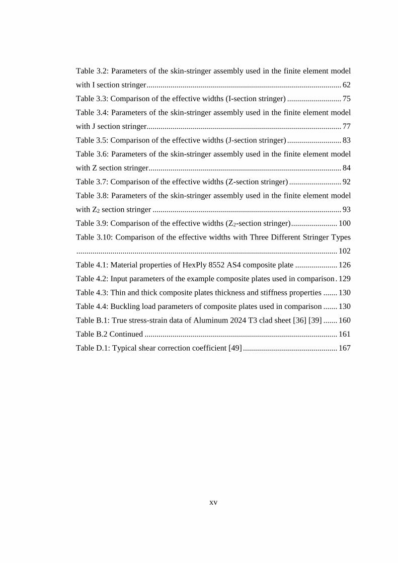
LIST OF TABLES

TABLES

Table 2.1: Definition of the constraints for the simply supported panel .................... 21

Table 2.2: Definition of the constraints for the clamped panel .................................. 21

Table 2.3: Material Properties of Aluminum 2024-T3 Clad Sheet ............................ 22

Table 2.4: Input parameters of the skin panels used in script .................................... 22

Table 2.5: Critical buckling stress results for various element sizes ......................... 26

Table 2.6: Input parameters of the skin-stringer assembly used in the finite element

model .......................................................................................................................... 33

Table 2.7: FEA input parameters for additional analyses for skin-stringer assemblies

with ‘J' type stringer ................................................................................................... 49

Table 2.8: Buckling coefficients of skin-stringer assemblies with J type stringers / FEA

results/ RS results / ANN results ................................................................................ 50


with ‘Z' type stringer .................................................................................................. 51

Table 2.10: Buckling coefficients of skin-stringer assemblies with Z type stringers /

FEA results/ RS results / ANN results ....................................................................... 52


with ‘T' type stringer .................................................................................................. 53

Table 2.12: Buckling coefficients of skin-stringer assemblies with T type stringers /

FEA results/ RS results / ANN results ....................................................................... 54

Table 3.1: Input parameters of the unstiffened skin panel used to verify stiffened panel

edge condition ............................................................................................................ 59

xv

Table 3.2: Parameters of the skin-stringer assembly used in the finite element model

with I section stringer ................................................................................................. 62

Table 3.3: Comparison of the effective widths (I-section stringer) ........................... 75


with J section stringer................................................................................................. 77

Table 3.5: Comparison of the effective widths (J-section stringer) ........................... 83


with Z section stringer ................................................................................................ 84

Table 3.7: Comparison of the effective widths (Z-section stringer) .......................... 92


with Z2 section stringer .............................................................................................. 93

Table 3.9: Comparison of the effective widths (Z2-section stringer) ....................... 100

Table 3.10: Comparison of the effective widths with Three Different Stringer Types

.................................................................................................................................. 102

Table 4.1: Material properties of HexPly 8552 AS4 composite plate ..................... 126

Table 4.2: Input parameters of the example composite plates used in comparison . 129

Table 4.3: Thin and thick composite plates thickness and stiffness properties ....... 130

Table 4.4: Buckling load parameters of composite plates used in comparison ....... 130

Table B.1: True stress-strain data of Aluminum 2024 T3 clad sheet [36] [39] ....... 160

Table B.2 Continued ................................................................................................ 161

Table D.1: Typical shear correction coefficient [49] ............................................... 167

xvi

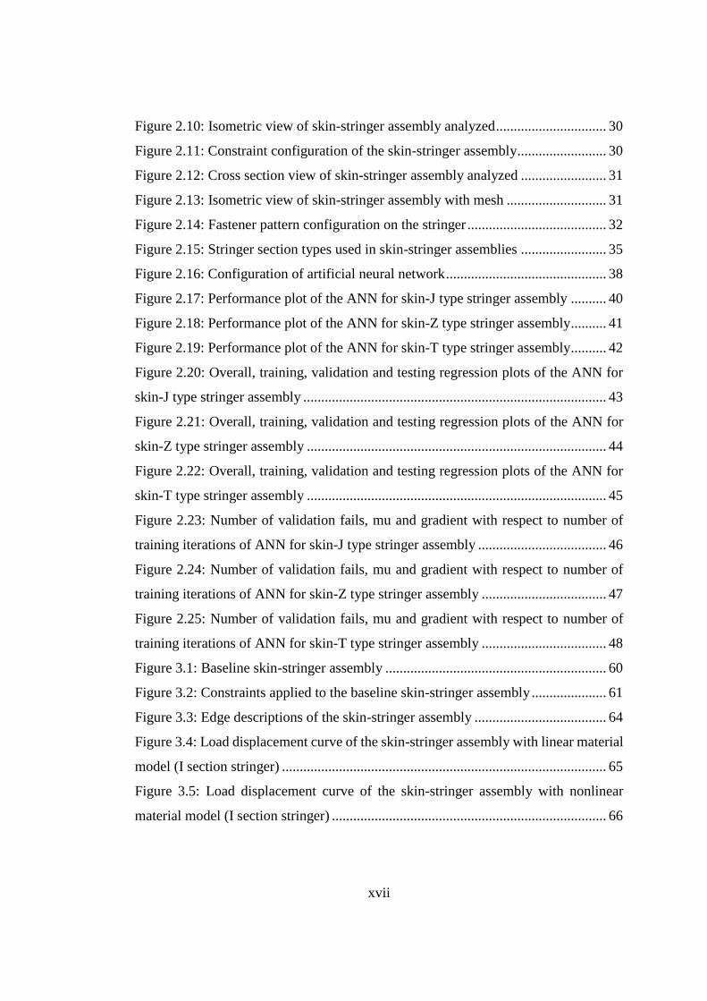
LIST OF FIGURES

FIGURES

Figure 1.1: Thin fuselage stiffened panel ..................................................................... 2

Figure 1.2: Load distribution in the skin-stringer assembly before and after buckling

[1] ................................................................................................................................. 4

Figure 1.3: Top view of compressive loaded skin-stringer assembly ........................ 12

Figure 1.4: Load distribution before the panel buckling [1] ...................................... 12

Figure 1.5: Load distribution after the panel buckling [1] ......................................... 12

Figure 2.1: Definition of different geometrical parameters of the flat panels and the

coordinate system ....................................................................................................... 20

Figure 2.2: Compressive load demonstration for the single panel case ..................... 23

Figure 2.3: Shear load demonstration for the single panel case ................................. 23

Figure 2.4: View of sample single panel model with all edges simply supported under

compressive loading ................................................................................................... 24

Figure 2.5: The critical buckling stress with respect to element number of flat panel

.................................................................................................................................... 25

Figure 2.6: Comparison of compressive buckling charts for flat rectangular panels with

simply supported loaded and unloaded edges ............................................................ 27

Figure 2.7: Comparison of compressive buckling charts for flat rectangular panels with

clamped loaded and unloaded edges .......................................................................... 27

Figure 2.8: Comparison of shear buckling charts for flat rectangular panels with simple

supported loaded and unloaded edges ........................................................................ 28

Figure 2.9: Comparison of shear buckling charts for flat rectangular panels with

clamped loaded and unloaded edges .......................................................................... 28

xvii

Figure 2.10: Isometric view of skin-stringer assembly analyzed ............................... 30

Figure 2.11: Constraint configuration of the skin-stringer assembly ......................... 30

Figure 2.12: Cross section view of skin-stringer assembly analyzed ........................ 31

Figure 2.13: Isometric view of skin-stringer assembly with mesh ............................ 31

Figure 2.14: Fastener pattern configuration on the stringer ....................................... 32

Figure 2.15: Stringer section types used in skin-stringer assemblies ........................ 35

Figure 2.16: Configuration of artificial neural network ............................................. 38

Figure 2.17: Performance plot of the ANN for skin-J type stringer assembly .......... 40

Figure 2.18: Performance plot of the ANN for skin-Z type stringer assembly .......... 41

Figure 2.19: Performance plot of the ANN for skin-T type stringer assembly .......... 42

Figure 2.20: Overall, training, validation and testing regression plots of the ANN for

skin-J type stringer assembly ..................................................................................... 43


skin-Z type stringer assembly .................................................................................... 44


skin-T type stringer assembly .................................................................................... 45

Figure 2.23: Number of validation fails, mu and gradient with respect to number of

training iterations of ANN for skin-J type stringer assembly .................................... 46


training iterations of ANN for skin-Z type stringer assembly ................................... 47


training iterations of ANN for skin-T type stringer assembly ................................... 48

Figure 3.1: Baseline skin-stringer assembly .............................................................. 60

Figure 3.2: Constraints applied to the baseline skin-stringer assembly ..................... 61

Figure 3.3: Edge descriptions of the skin-stringer assembly ..................................... 64

Figure 3.4: Load displacement curve of the skin-stringer assembly with linear material

model (I section stringer) ........................................................................................... 65

Figure 3.5: Load displacement curve of the skin-stringer assembly with nonlinear

material model (I section stringer) ............................................................................. 66

xviii

Figure 3.6: FE view of skin-stringer assembly with nonlinear material model (I section

stringer) at local buckling starting point .................................................................... 66

Figure 3.7: FE view of skin-stringer assembly with nonlinear material model (I section

stringer) at collapse point ........................................................................................... 67

Figure 3.8: Comparison of load displacement curves of models with linear and

nonlinear material properties (I section stringer section) ........................................... 67

Figure 3.9 Top view of skin-stringer assembly under compressive loading .............. 68

Figure 3.10: Actual load distribution in the post-buckled stage [1] ........................... 69

Figure 3.11: Equivalent load distribution using the concept of effective width [1] ... 69

Figure 3.12: Load distribution in the skin-stringer assembly with the linear material

model just before the skin buckling (I section stringer) ............................................. 70


model at the collapse displacement (1.736 mm) of the nonlinear material model case

(I section stringer) ...................................................................................................... 71

Figure 3.14: Closed view of load distribution in the skin-stringer assembly with the

linear material model at the collapse displacement (1.736 mm) of the nonlinear

material model case (I section stringer) ..................................................................... 71

Figure 3.15: Load distribution in the skin-stringer assembly with the nonlinear material

property just before the skin buckling (I section stringer) ......................................... 72

Figure 3.16: Load distribution in the skin-stringer assembly with nonlinear material

property at the collapse displacement of 1.736 mm (I section stringer) .................... 73

Figure 3.17: Comparison of the load distribution in the skin-stringer assemblies with

linear and nonlinear material properties (I section stringer) ...................................... 73

Figure 3.18: Stringer section types used in this study ................................................ 76

Figure 3.19: Load displacement curve of the skin-stringer assembly with linear

material model (J section stringer) ............................................................................. 78


material model (J section stringer) ............................................................................. 79


model just before the skin buckling (J section stringer) ............................................. 79

xix


model the collapse displacement (1.726 mm) of the nonlinear material model case (J

section stringer) .......................................................................................................... 80


model just before the skin buckling (J section stringer) ............................................ 81


model at the collapse displacement of 1.726 mm (J section stringer) ....................... 81

Figure 3.25: Comparison of the load distribution of skin-stringer assemblies with linear

and nonlinear material properties (J-section stringer) ................................................ 82

Figure 3.26: Single and double fastener configurations with Z section stringer ....... 83

Figure 3.27: Load-displacement curve of the skin-stringer assembly with linear

material model (Z section stringer) ............................................................................ 85

Figure 3.28: Buckled shape of mid panel before and after views of second drop point

.................................................................................................................................... 86


material model (Z section stringer) ............................................................................ 87


nonlinear material properties (Z section stringer) ...................................................... 87


model just before the skin buckling (Z-section stringer) ........................................... 88

Figure 3.32: Load distribution in the panel with the linear material model at the

compressive collapse displacement of 0.823 mm (Z- section stringer) ..................... 89

Figure 3.33: Load distribution of the model with nonlinear material property just

before the skin buckling (Z-section stringer) ............................................................. 89

Figure 3.34: Load distribution of the model with nonlinear material property at the

compressive displacement of 0.823 mm (Z stringer section type)............................. 90

Figure 3.35: Comparison of load distribution of models with linear and nonlinear

material properties (Z-section stringer) ...................................................................... 91

Figure 3.36: Load-displacement curve of the skin-stringer assembly with linear

material model (Z2 section stringer) ........................................................................... 94

xx


material model (Z2 section stringer) ........................................................................... 95


nonlinear material properties (Z2 section stringer) ..................................................... 96


model just before the skin buckling (Z2-section stringer) .......................................... 96

Figure 3.40: Load distribution in the panel with the linear material model at the

compressive collapse displacement of 1.637 mm (Z2-section stringer) ..................... 97

Figure 3.41: Load distribution of the model with nonlinear material property just

before the skin buckling (Z2-section stringer) ............................................................ 97

Figure 3.42: Load distribution of the model with nonlinear material property at the

compressive displacement of 1.637 mm (Z2 stringer section type) ........................... 98

Figure 3.43: Comparison of load distribution of models with linear and nonlinear

material properties (Z2-section stringer) .................................................................... 99

Figure 3.44: Comparison of load carrying capacity of skin-stringer assemblies with I,

J, Z and Z2 section stringers (Nonlinear material properties) .................................. 101

Figure 3.45: Comparison of load distribution of skin-stringer assemblies with I, J, Z

and Z2 section stringers (Nonlinear material properties) ......................................... 101

Figure 4.1: Undeformed and deformed geometries of an edge of a plate under the

Kirchhoff assumptions [41] ...................................................................................... 107

Figure 4.2: Undeformed and deformed geometries of an edge of a plate under the

assumptions of the first-order plate theory [43]. ...................................................... 111

Figure 4.3: Plate with uniaxial compression load [41]. ............................................ 115

Figure 4.4: Definition of different geometrical parameters of the composite panels and

the coordinate system ............................................................................................... 125

Figure 4.5: Compressive buckling coefficients for composite plates with simply

supported loaded and unloaded edges (Ply orientation: 0°/0°𝑆) ............................. 131


supported loaded and unloaded edges (Ply orientation: 0°/90°𝑆) ........................... 131

xxi


supported loaded and unloaded edges (Ply orientation: 45°/0°/−45°/90°𝑆) ........ 132

Figure 4.8: Compressive buckling coefficients for composite plates with clamped

loaded and unloaded edges (Ply orientation: 0°/0°𝑆) ............................................. 132


loaded and unloaded edges (Ply orientation: 0°/90°𝑆) ........................................... 133


loaded and unloaded edges (Ply orientation: 45°/0°/−45°/90°𝑆)......................... 133

Figure 4.11: Compare of compressive buckling coefficients with all edges simply

supported (Ply orientation: 0°/0°𝑆, thickness of plate=1.04 mm) .......................... 134


supported (Ply orientation: 0°/0°𝑆, thickness of plate=2.08 mm) .......................... 135


supported (Ply orientation: 0°/90°𝑆, thickness of plate=1.04 mm) ........................ 135




supported (Ply orientation: 45°/0°/−45°/90°𝑆, thickness of plate=2.08 mm) ..... 136


supported (Ply orientation: 45°/0°/−45°/90°𝑆, thickness of plate=4.16 mm) ..... 137

Figure 4.17: Compare of compressive buckling coefficients with all edges clamped

(Ply orientation: 0°/0°𝑆, thickness of plate=1.04 mm) ........................................... 137


(Ply orientation: 0°/0°𝑆, thickness of plate=2.08 mm) ........................................... 138


(Ply orientation: 0°/90°𝑆, thickness of plate=1.04 mm) ......................................... 138


(Ply orientation: 0°/90°𝑆, thickness of plate=2.08 mm) ......................................... 139


(Ply orientation: 45°/0°/−45°/90°𝑆, thickness of plate=2.08 mm) ...................... 139

xxii


(Ply orientation: 45°/0°/−45°/90°𝑆, thickness of plate=4.16 mm) ...................... 140


supported at the same plate thickness (2.08 mm) ..................................................... 140

Figure 4.24: Compare of compressive buckling coefficients with all edges clamped at

the same plate thickness (2.08 mm) ......................................................................... 141

Figure 4.25: Example view of first buckled mode shape of plate with all edges simply

supported (Ply orientation: 0°/0°𝑆, thickness of plate=2.08 mm) ........................... 142




supported (Ply orientation: 45°/0°/−45°/90°𝑆, thickness of plate=2.08 mm) ...... 143

Figure B.1: Material properties of aluminum 2024 T3 clad sheet [36] .................... 159

Figure B.2: True stress-strain graph of Aluminum 2024 T3 clad sheet [36] [39] .... 160

Figure C.1: Buckling factors for several edge conditions [1] .................................. 164

Figure D.1: Cross section view of a laminate .......................................................... 167

Figure D.2: A differential element with in-plane force resultants [42] .................... 168

Figure D.3: A differential element with moment resultants, shear force resultants and

applied transverse forces [42] .................................................................................. 169

Figure D.4: Force projection of in-plane normal and shear forces in the z direction

[50] ........................................................................................................................... 170

Figure E.1: Material properties of HexPly 8552 AS4 at dry and room temperature [51]

.................................................................................................................................. 173

xxiii

LIST OF ABBREVIATIONS

ANN Artificial neural network

𝐴𝑒𝑓𝑓 Area under the load distribution curve of skin

CLPT Classical laminated plate theory

𝐸 Elastic modulus

𝐸𝑐 Compressive elastic modulus

𝐹𝑐𝑟𝑖𝑝 Stringer crippling allowable stress

𝐹𝑐𝑦 Yield compressive allowable stress

𝐹𝑙𝑏 Stringer local buckling allowable stress

𝐹𝑚𝑎𝑥 Skin maximum stress in the post-buckling stage

𝐹𝑠𝑡𝑟 Stringer Stress

𝐹𝑡𝑢 Tensile ultimate allowable stress

FE Finite element

FEA Finite element analysis

FEM Finite element model

FSDT First order shear deformation theory

𝑘 Buckling coefficient

𝑘𝑒𝑓𝑓 Effective width constant

𝑙𝑙𝑓 Lower flange width of stringer

𝑙𝑥 Skin length in the x direction

𝑙𝑦 Skin length in the y direction

𝑚𝑚 Millimeter

𝑀𝑃𝑎 Megapascal

𝑛𝑐 Ramberg-Osgood factor of plasticity in compression

𝑁 Newton

xxiv

𝑁𝑎𝑝𝑝 Compressive shell edge load

NACA National advisory committee for aeronautics

NASA National aeronautics and space administration

RS Response surface

𝑡 Skin thickness

𝑢𝐹𝐸 Applied displacement

𝑢𝑐𝑟 Critical displacement

𝑣 Poisson ratio

𝑤𝑒𝑓𝑓 Effective width of skin

𝜎𝑐𝑟 Critical buckling stress

𝜆𝐹𝐸 First eigenvalue obtained from finite element analysis

1

CHAPTERS

CHAPTER 1

1. INTRODUCTION

1.1. Motivation of the Study

Stiffened thin panels are very common and vital structural elements in aerospace

structures because of the weight and stiffness advantages that they provide. Stiffened

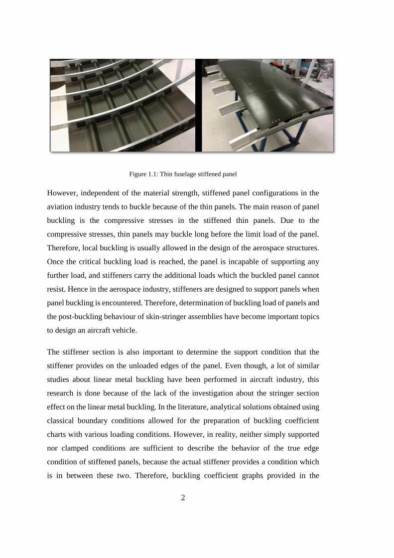
panels, as shown in Figure 1.1, are built by thin walled panels supported by stiffeners.

Up to 1980s, stiffened panels are only made from Aluminum material. The reason is

the construction of aluminum based structure is feasible by verified design methods,

validated analysis tools with an enormous measure of test outputs. In addition,

aluminum based structures’ strength properties and failure scenarios are studied since

the end of the eighteenth century. However, in recent decades, advanced materials like

fibrous carbon composites have attracted great interest for use in aerospace industry

owing to their favorable properties, such as high specific strength and stiffness. For

the last thirty years, through the onset of composite materials, many studies have been

performed to replace the conventional aluminum based shell structure with composite

materials.

2

Figure 1.1: Thin fuselage stiffened panel

However, independent of the material strength, stiffened panel configurations in the

aviation industry tends to buckle because of the thin panels. The main reason of panel

buckling is the compressive stresses in the stiffened thin panels. Due to the

compressive stresses, thin panels may buckle long before the limit load of the panel.

Therefore, local buckling is usually allowed in the design of the aerospace structures.

Once the critical buckling load is reached, the panel is incapable of supporting any

further load, and stiffeners carry the additional loads which the buckled panel cannot

resist. Hence in the aerospace industry, stiffeners are designed to support panels when

panel buckling is encountered. Therefore, determination of buckling load of panels and

the post-buckling behaviour of skin-stringer assemblies have become important topics

to design an aircraft vehicle.

The stiffener section is also important to determine the support condition that the

stiffener provides on the unloaded edges of the panel. Even though, a lot of similar

studies about linear metal buckling have been performed in aircraft industry, this

research is done because of the lack of the investigation about the stringer section

effect on the linear metal buckling. In the literature, analytical solutions obtained using

classical boundary conditions allowed for the preparation of buckling coefficient

charts with various loading conditions. However, in reality, neither simply supported

nor clamped conditions are sufficient to describe the behavior of the true edge

condition of stiffened panels, because the actual stiffener provides a condition which

is in between these two. Therefore, buckling coefficient graphs provided in the

3

literature are not sufficient to use effectively in aerospace structures which

predominantly have stiffened thin walled panels. To have an optimum skin-stringer

assembly design, the structure must be modelled with the correct boundary conditions.

Post buckling behaviour of skin-stringer assemblies is also very crucial in aerospace

structures since local buckling of panels may be allowed in some design practices. As

mentioned before, once the critical buckling load is reached, the skin of a stiffened

panel loses its load carrying capacity and stiffeners carry the additional loads which

the buckled skin cannot carry. Besides the stiffeners, the effective section of the skin

panel also carries small proportion of the load applied, but depending on the skin-

stringer assembly the load carried by the skin varies. Load carrying capacity of a

stiffened panel is significantly affected by the design of the skin-stringer assembly.

Until the local buckling of the skin, both middle portion of skin and skin part at the

stringer location have the same stress level. After the local buckling of the skin panel,

which is referred to as the post-buckling stage, stress distribution over the skin panel

is nonlinear. Because of the buckled skin, that is no longer effective to carry the

additional compressive load, the additional load is redistributed to the adjacent stiffer

structural members which are stringers and frames in semi-monocoque structures.

Figure 1.2 shows the actual load distribution over the panel before, after buckling and

equivalent load distribution over the panel after buckling. In the classical approach, in

order to handle the non-uniform load over the skin panel after buckling, equivalent

width concept has been used commonly. Equivalent width pertains to the part of the

skin that is assumed to carry the uniform load. However, in this method, effect of

material nonlinearity is not taken into consideration. Same as the linear buckling

method, classical boundary condition assumption is made in the literature in

conjunction with the effective width method. However, in reality, classical boundary

conditions are not sufficient to describe the behavior of the true edge condition of

stiffened panels, because the actual stiffener provides a condition which is in between

these two. Therefore, effective width formulation provided in the literature is not

sufficient to use effectively in aerospace structures. To measure the true load capacity

of the skin-stringer assembly design, the structure must be modelled with the correct

boundary conditions in the post-buckling stage.

4

Figure 1.2: Load distribution in the skin-stringer assembly before and after buckling [1]

Furthermore, for composite panels, buckling charts are required to for faster evaluation

of buckling response of composite panels. To save the time in the aviation industry,

parametric studies has to be done for specific configurations which are commonly used

in this industry.

5

1.2. Scope of the Study

In this study, the two parts of this research focuses on the buckling and post-buckling

behaviour of the unstiffened and stiffened panels applied to uniaxial compressive

loadings. In the first part of the research, a database is prepared for the buckling

coefficients of the selected skin-stringer combinations. Then, the differences between

the buckling coefficients of the real skin-stringer geometries and the analytically

determined buckling coefficients which rely on classical boundary conditions are

identified. Created database is processed with the ANN and RS methods to reach the

result quickly compare to finite element analysis. In the second part of the research,

load distribution of the skin-stringer assembly in the post-buckling stage is

investigated. Stringer section effect on the load distribution and load capacity of the

skin-stringer assembly is the main objective of the second part of the thesis study. In

the third part of the thesis, buckling coefficient charts for unstiffened composite panels

are obtained. To restrict the panel edges, classical boundary conditions are used in the

modelling of the unstiffened panel. In this part, each chart has a specific laminate

orientation. These charts are obtained with 3 different methods. These methods are the

classical laminate plate theory (CLPT), first order shear deformation theory (FSDT)

and finite element analysis. Analytical methods’ results are compared with the finite

element results in this part.

6

1.3. Content of the Study

• In Chapter 2, brief information about buckling formulation and buckling

procedure in finite element analysis are given. Buckling phenomenon for

unstiffened panels is explained and the buckling coefficient graphs are

described. Determination of buckling coefficients of unstiffened panels with

classical boundary conditions by finite element analysis is described. After the

verification of unstiffened panel boundary conditions with analytical solution,

stiffened panel modelling is explained. Using this modelling technique, 2000

analysis are done for each stringer section type. At the end of the chapter,

artificial neural network and response surface for fast determination of

buckling coefficients are constructed.

• In Chapter 3, firstly, brief information about post-buckling stage is given. In

addition, determination of the baseline skin-stringer assembly is explained.

Then, post-buckling analysis of skin-stringer assemblies using linear and

nonlinear material models is studied. Methodology of effective width

calculation by the finite element solution and empirical solution is presented.

At the end of the chapter, results for different stringer section types are

presented.

• In the Chapter 4, firstly, brief information and formulation about the classical

laminated plate theory (CLPT) and the first order shear deformation theory

(FSDT) is given. Buckling analysis of specially orthotropic plates under the

compressive load using CLPT and FSDT is explained. Finite element model of

the composite plates is described. Using the finite element model results,

buckling coefficient charts are obtained for each ply orientation and thickness

of composite plates. Finally, buckling results obtained by the CLPT and FSDT

theories are presented and comparisons are made with finite element results.

• In the Chapter 5, the results are discussed. In addition, summary and the future

work of the study are given in this part.

7

1.4. Literature Survey

Stiffened thin panel configuration is considered to be very efficient way to carry the

loads in aerospace structures because of the weight and stiffness advantages they

provide. Accurate analysis of buckling and post-buckling behaviour of skin-stringer

assemblies used in aerospace structures is very crucial, because local buckling is

permitted in some designs practices of aerospace structures.

In the first and second phases of the thesis study, buckling and post buckling behaviour

of the stiffened thin panel with metallic material properties are investigated. In the

literature, there are many studies about buckling and post buckling phenomena. A few

of them are mentioned in this sub-chapter.

In theory, buckling refers to the loss of stability of a component and it is commonly

independent from the material strength. In practically, due to compressive stresses in

the stiffened thin panel, thin panel may be buckled long before the limit load of the

panel. Therefore, local panel buckling is usually allowed in the design of the aerospace

structures.

Study about the plate buckling started in the early of the 19th century. Claude-Louis

Navier derived the stability equation for a rectangular thin plate. This derivation is

based on Gustav Robert Kirchhoff assumptions in 1822 [2]. In 1891, the critical

buckling stress equation for a rectangular thin plate with simply supported edge

condition under uniaxial compression load is formulated by Bryan [2]. In his study,

energy method is used to determine the critical load. One of the known detailed study

about the buckling is written in the NACA Handbook of Structural Stability document

[3]. This handbook presents a rather comprehensive review and compilation of theories

and experimental data relating to the buckling phenomena. The various factors

governing the buckling of flat plates are reviewed and results are summarized in

comprehensive series of charts and tables in this handbook. In 1925, Timoshenko [4]

also solved the same problem using another method. He assumed the plate to be

buckled into several sinusoidal half waves in the direction of compression. He also

explored the buckling of uniformly compressed rectangular plates that are simply

8

supported along the edges perpendicular to the direction of applied load and other two

edges subjected to various end conditions. Results have been reported in standard texts

[4, 5, 6].

In the aerospace industry, stiffeners are designed to support panels when panel

buckling is encountered. The stiffener section is important to determine the support

condition that the stiffener provides on the unloaded edges of the panel. In the

literature, analytical solutions obtained using classical boundary conditions allowed

for the preparation of buckling coefficient charts with various loading conditions [1].

These charts also show the change in buckled shape as the boundary conditions are

altered on the unloaded edges from free to fully restraint condition. Classical boundary

conditions are commonly known as free, simply supported and clamped. In reality,

neither simply supported nor clamped conditions are sufficient to describe the behavior

of the true edge condition of stiffened panels, because the actual stiffener provides a

condition which is in between these two.

In airframe structural design data book [6], various wing design loads are given as

shears, bending moments and torsion which results from air pressures and inertia

loadings. In addition to these types of loads, buckling coefficients are given for each

boundary conditions and geometric panel description.

In the study of the Paul et al. [2], a standard transport aircraft wing is considered and

buckling analysis is carried out. The initial design is found to buckle. So, several

design modifications were made to make the design safe against buckling. In this

study, FE analysis and theoretical study are performed to get realistic results in the

wing buckling analysis. Yu [7] has studied the buckling behavior of rectangular plates

subjected to intermediate and end loads. He considered both elastic buckling and

plastic buckling behavior of plates. Plate considered is simply supported along two

opposite edges that are parallel to the direction of applied loads. The two edges may

take any other combination of clamped, simply supported and free edge boundary

conditions. Study also investigates the effect of various plate aspect ratios,

intermediate load positions, boundary conditions on buckling factors [7]. In the study

of the Muameleci [8], linear and nonlinear buckling analyses of plates with and without

9

cut-out using finite element method are investigated. Various classical boundary

conditions and loading conditions are used to model the shear web beam structures.

The main point of this study is the investigate the buckling behaviour of plates but also

the capabilities of the MSC Nastran and ABAQUS finite element tools for performing

linear and nonlinear buckling analyses. Riks [9] has applied finite strip method for the

calculation of the buckling load of stiffened panels in wing box structures. This article

describes the implementation of the finite strip method. The finite strip method extends

the scope of the analysis of the determination of the post buckling stiffness of the

panels. Finite strip model (one dimensional) is the simplification of finite element

model (two dimensional). Some of the computer implementations of the finite strip

method are BUCLASP [10] and VIPASA [11]. In the study of Riks, the method used

for the analysis of the finite strip model is PANBUCK which has the ability to analyze

the initial post buckling behavior too.

In the literature, there have been many studies on the post-buckling behaviour of skin-

stringer assemblies. The paper of Murphy [12] reports on the development of a

modeling approach to increase the accuracy of the global model, accounting variations

in stiffness due to nonlinear structure behavior. In the study of Lync and Sterling [13],

a finite element methodology has been presented for the compressive post-buckling.

In this study, test data are compared to results of four different finite element modelling

approaches for the skin-stringer assembly. Moreover, in the study of Weimin et al.

[14], experimental and analytical study results of post buckling simulation of an

integral aluminum fuselage stiffened panel have been presented. In this study, load is

applied as axial compression load and the panel is a curved panel. Rhodes [15]

examined some of the research on the elastic and plastic post-buckling behaviour of

plates and plate like structures. In this study, post buckling behaviour of individual

thin plates is governed by non-linear differential equations set up by Von Karman. In

the study of the Eirik Byklum et al. [16], a computational model for the analysis of

global buckling and post-buckling of stiffened panels has been derived. The model

was developed as part of a tool for buckling phenomenon of stiffened panels. It is

formulated using large deflection plate theory and energy principles. Deflections are

assumed in the form of trigonometric function series. In addition, the principle of

10

stationary potential energy is used for deriving the equilibrium equations. For the

loading case, lateral pressure is accounted for by taking the deflection as a combination

of a clamped and a simply supported deflection mode. The global buckling model is

based on Marguerre’s nonlinear plate theory, by deriving a set of anisotropic stiffness

coefficients to account for the plate stiffening. Local buckling is treated in a separate

local model developed. The anisotropic stiffness coefficients used in the global model

are derived from the local analysis. Together, the two models provide a tool for

buckling phenomena of stiffened panels. Any combination of biaxial in-plane

compression or tension, shear, and lateral pressure are analyzed in this study. The

procedure is semi-analytical in the sense that all energy formulations are derived

analytically, while a numerical method is used for solving the resulting set of

equations, and for incrementing the solution. The load deflection curves produced by

the proposed model are compared with results from nonlinear FEM. In the study of the

Kopecki et al. [17], the results of experiments and numerical analyses of thin-walled

shells used as components of aircraft structures are presented. In this study, integral

rigs are used to stiffened the structure. A comparative analysis has been carried out

between the suggested design solution and the reference structure. In the experimental

part of the study, an optical scanner with digital image correlation has been used.

Nonlinear numerical analyses have been carried out with the use of software based on

the finite element method. The suggested method for verifying the results of non-linear

numerical analysis by applying the principle of equivalent solutions seems to be

effective, and the obtained results are sufficiently credible. This constituted the

foundation for carrying out an initial comparative analysis of the physical properties

of the load-bearing structures in question. In the light of this analysis, the solution

based on the use of integral ribs seems to be very promising from the point of view of

its application in load-bearing aircraft structures.

The study of the Graciano et al. [18] is aimed at studying the influence of initial

geometric imperfections on the post-buckling behavior of longitudinally stiffened

plate girder webs subjected to patch loading. A sensitivity analysis is conducted herein

using two approaches (deterministic and probabilistic) in order to investigate the effect

of imperfection shape and amplitude on both, the post-buckling response and ultimate

11

strength of plate girders under patch loading. According to the results from the

deterministic approach, the amplitude of the imperfections in most cases leads to a

reduction in patch loading resistance. This sensitivity analysis is performed by means

of nonlinear finite element analysis. At first, the initial shape imperfections are

modeled using the buckling mode shapes resulting from an eigenvalue buckling

analysis. Afterwards, the amplitude of the buckling shapes for the various modes is

varied, and then introduced in the nonlinear analysis. The results also showed a more

complex interaction between the imperfection shapes and the computed resistances.

Nevertheless, the shape of the initial imperfection that results in the lowest strength

for a girder differs for each size of imperfection and stiffener location. It is also

important to point out that initial imperfection for patch loaded girder webs can be

modeled using a shape resembling either the first eigen mode or a sinus-wave.

Load carrying capacity of a stiffened panel is vital topic and significantly affected by

the design of the skin-stringer assembly. Until the local buckling of the skin, both skin

and stringers have the same stress level. After the local buckling of the skin panel,

which is referred to as the post-buckling stage, stress distribution over the stiffened

panel is nonlinear. Because of the buckled skin, that is no longer effective to carry the

additional compressive load, the additional load is redistributed to the adjacent stiffer

structural members which are the stringers and frames in semi-monocoque structures.

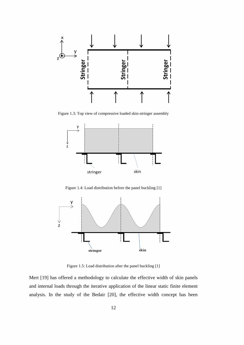
Figure 1.3 shows the top view of skin-stringer assembly under compressive loading.

Figure 1.4 and Figure 1.5 show the load distribution over the panel before and after

buckling, respectively. As shown in Figure 1.5, the section of skin panels, at the

stiffener attachment lines, do not buckle. This means that the stiffener and skin still

have the same strain level at the attachment line. However, at the mid-panel, skin panel

can no longer carry the additional load after the panel buckling [19]. In the classical

approach, in order to handle the non-uniform load over the skin panel after buckling,

equivalent width concept has been used commonly [1]. Equivalent width pertains to

the part of the skin that is assumed to carry uniform load. In the classical approach,

effective width concept has been widely used in the post-buckling analysis of skin-

stringer assemblies [1, 6].

12

Figure 1.3: Top view of compressive loaded skin-stringer assembly

Figure 1.4: Load distribution before the panel buckling [1]

Figure 1.5: Load distribution after the panel buckling [1]

Mert [19] has offered a methodology to calculate the effective width of skin panels

and internal loads through the iterative application of the linear static finite element

analysis. In the study of the Bedair [20], the effective width concept has been

13

investigated since it is widely used in engineering practice for the computation of

ultimate strength of slender members. The paper of Osama [20] presents analytical

closed form expressions for the computation of effective width of thin plates under

non-homogeneous in-plane loading. The longitudinal edges are assumed to be straight

and free to translate in the plane of the plate. In this study, it is considered that the

proposed expressions are very useful for limit state design of slender I-sections of

beam columns or channel sections under this general type of loading. The unloaded

edges were assumed to be straight and free to translate in the plane of the plate. The

compatibility differential equation is first solved analytically to obtain a closed form

solution for the stress function. The equilibrium differential equation is then solved

approximately using the Galerkin method. Based on the characteristics of the post-

buckling stress field, analytical expressions for the effective width were proposed. The

sensitivity and mechanics of the effective width to the stress gradient parameter was

shown. The resulting analytical expressions have simple forms, suitable for hand-

calculation and avoid the cost and effort that any numerical non-linear analysis may

require. In the study of the Dannemann [21], the author presents a complementary

criterion for effective width which is based on tests performed on thin trapezoidal

sheets, when flanges buckle in the elastic range. This method compares well with the

observed behavior and ultimate strength of test specimens. The author's suggestion is

that for inelastic buckling the AISI and correlated design codes are valid but when

sheets are very slender and they buckle elastically, a modified effective width criterion

has to be applied. This proposed method not only shows excellent correlation with

tests, but also facilitates a rational agreement between stiffened and unstiffened flange

behavior when plates are very thin, fulfilling physical requirements not accomplished

by the classical effective width method. In addition, this method allows the calculation

of the post buckling strength of flanges and webs by using physically measurable

values instead of empirical parameters. The effective width concept is a classical

resource for representing local buckling effects on stiffened flat flanges. There has

been a great deal of testing and investigations on this matter. The most important

contribution to the adoption of this method was proposed in Winter [22] included by

AISI in their Specification of Light Gage Structural Members of·1946. As known, the

14

effective width concept is based on Von Karman's proposition of 1932 where the

uneven stress distribution of buckled flanges was replaced by evenly stressed fictitious

strips along the corners of the flanges. This structural artifice has shown excellent

results in design practice of metal structures. A great number of tests in different

countries confirm the accuracy of this method mainly in plates buckling in the inelastic

range, but from time to time some discrepancies have been detected and published for

flanges buckling elastically.

Finite element modelling and analysis of the actual skin-stringer assembly takes very

long time in the design optimization process. One of the efficient method to optimize

the structure is the artificial neural network (ANN). In the literature, there are a few

studies about the prediction of the failure modes using ANN.

A study of optimization of a compression member conducted by Sheidaii and

Bahraminejad [23] is an example of the use of ANN in optimization. In the study, load-

displacement relation of different types of columns was obtained using analytical

methods. The results were utilized to form a data set to train an ANN. Similar to the

study of Sheidaii et al., ANN is used to predict bolt reaction force and average

equivalent flange stress without using finite element model in the study of Yıldırım

[24]. In this study, a bolted flange design tool is created by using ANN. As the general

sense, a data set was created with finite element model parameters and corresponding

analysis results. The data set was used in training, validating and testing of ANN. At

the end, the ANN results were compared with FEA and analytical methods.

Comparison results are sufficient to use the ANN tool in the further design of bolted

flanges. Another optimization study which is written by Gomes et al. [25] was

conducted on anisotropic laminated composites. In this study a genetic algorithm and

two ANNs were used to optimize the design of a laminated composite. It was stated

that the use of these methods leads to accurate enough solutions and decrease the time

required for the design process. Gajewski et al. [26] studied the use of the ANN for

the optimization of a thin-walled structure. FEA results of the structure were used to

train the ANN. This study is another example that the ANN is an appropriate tool in

design and analysis of airframe structures.

15

Buckling and collapse loads of panels have also been studied to create analysis tools

based on ANN. Sadovský and Soares [27] obtained post-buckling strength of a thin

rectangular plate by creating an ANN as a function of initial imperfections. The created

ANN was found to be able to provide reasonable collapse load results. The post-

buckling optimization by using ANN was utilized for stiffened panels in a study of

Lanzi and Giavotto [28]. The study used different optimization methods including

ANN to optimize composite stiffened panels subjected to axial compression. The

results were verified by tests and it was seen that accurate results can be obtained for

both the buckling load and the collapse load. Mallela and Upadhyay [29] also used the

ANN to calculate the buckling load. The study was focused on buckling load

prediction of composite stiffened panels working under shear loads. FEA results for

different composite structures were collected in a database to train an ANN tool. An

efficient tool that can be used in optimization was created in the study. In the study of

Cankur [30], an ANN based structural analysis tool to predict the buckling and collapse

loads of the stiffened panels is created. The ANN is trained by using a database created

with the input parameters and the FEA results of 1440 metallic skin-stringer

assemblies subjected to uniaxial compression. The first buckling load and the collapse

load are extracted from the nonlinear FEA results of the assembly. Using the results of

the same analysis for the buckling and the collapse load, the time required for the

generation of the training database is significantly reduced. Also, the first buckling

load is obtained with an enhanced accuracy by using nonlinear analysis instead of

linear buckling analysis.

In the final phase of the thesis study, buckling behaviour of the unstiffened thin

composite panels is studied. In the last three decades, there have been many studies

performed on composite buckling. Same as the metallic part, some of the studies about

the composite buckling in the literature are presented in this sub-chapter.

In the study of the Yang [31], CLPT and FSDT analysis methods are investigated for

composite plate buckling. These methods are developed for plates subjected to uniaxial

compression loading and both simply supported and clamped edge plates have been

studied. Analysis methods for plates subjected to biaxial compression loading, in-

16

plane shear loading and combined loading, with simply supported edges have been

studied. To validate the analysis methods, FE analyses is performed using ANSYS.

The methods based on FSDT give a better estimation than CLPT. According to Qiao,

these methods are suitable for thin and moderately thick plates. Furthermore, in this

study, the considered methods are limited to linear case. In the study of the Masood et

al. [32], a composite skin-stringer panel was designed for compression testing under

axial compression loads beyond initial skin buckling. The panel was fabricated using

Carbon/Epoxy prepreg through autoclave moulding process. A finite element model

was developed to predict the buckling and post-buckling response of the panel. Digital

Image Correlation captured the onset of skin buckling and deformations/mode shapes

in the post-buckled regime. Experimental observations were then correlated with

numerical simulations. In the post buckled regime, severe bending and twisting of the

skin and stringers were observed, resulting in complete loss of global axial stiffness of

the panel. It is investigated that stress at the post buckled regime in the panel could

lead to delamination, debonding or fiber failures. Local skin buckling is also confirmed

through strain measurements using a number of strain gages bonded on the panel skin.

In the study of the Abramovich and Weller [33], an extensive test series on circular

cylindrical laminated composite stringer-stiffened panels subjected to axial

compression, shear loading. The test program was an essential part of an ongoing effort

undertaken aiming at the design of low cost, low weight airborne structures that was

initiated. Test results on curved composite panels stiffened by J-stringers were

presented and discussed. Test results were compared with predictions obtained by an

in-house developed code and the commercial FE code ABAQUS. Accompanying

supporting calculations were presented as well; they were performed with a fast

calculation tool developed and based on the effective width method modified to handle

laminated circular cylindrical stringer-stiffened composite panels. In the study of

Möcker et al. [34], it is shown how the finite element code ABAQUS can be used for

an accurate and reliable prediction of the post-buckling behaviour. When performing

finite element simulations, a large amount of time is often needed to build up the finite

element model, in particular if the model consists of several parts with complex

geometries. For this reason, the preprocessing tool ABAQUS/CAE provides an

17

interface which allows the user to automate repetitive tasks. The main focus of this

paper is on discussing several modelling techniques that are used to enable a realistic

idealization of the physical problem and on presenting simulation results for an

exemplary structure. Based on this example, the influence of modelling details like

mesh density and geometric imperfections on the prediction of the failure load is

discussed.

18

19

CHAPTER 2

2. BUCKLING OF STIFFENED METALLIC FLAT PANELS

Buckling load highly depends on the boundary condition, loading type, material

property and geometric properties of the panel. In the literature, calculation of the

buckling load is limited with the classical boundary conditions [1, 6]. However, in

realistic cases, boundary conditions of the panel are provided by stiffeners on the

loaded and unloaded edge of the panel. To get realistic value of the buckling load,

finite element analyses (FEA) of the stiffened panel is necessary, but finite element

analysis is time consuming considering the preparation time required for the analysis

model and the analysis time required. ABAQUS is chosen in the finite element

modelling of the structures. ABAQUS is the commercial finite element software which

is commonly used in the aerospace industry. In this study, ABAQUS up to date version

6.14 is used in the finite element modelling. To find the buckling load in this study,

ABAQUS “buckling” step for the linear buckling analysis is utilized. In FEA, the

procedure of obtaining buckling eigenvalue is described in Appendix A.

In this chapter, it is aimed to prepare databases for the buckling coefficients of selected

metallic skin-stringer assemblies by means of parametric modeling approach via the

script language followed by automated finite element analysis. With this approach,

databases of buckling coefficients for skin-stringer assemblies can to be generated

similar to the available buckling coefficient charts for the panels which have classical

20

boundary conditions along the edges. Skin-stringer assemblies are established for T, Z

and J type stringers. For each skin-stringer type, a database is created. Using these

databases, the buckling load and the compression buckling coefficient of the skin-

stringer assembly can be obtained much faster than modeling and analyzing the skin-

stringer assembly by the finite element method. Thus, skin-stringer optimizations can

be performed very quickly. To construct the databases, numerous skin-stringer

assemblies are modeled with different sizes and types in ABAQUS 6.14. Database is

created by writing a script in Python 2.7 which is then used in ABAQUS to generate

the parametric models of the skin-stringer assemblies followed by automated finite

element analysis controlled by the Python script.

2.1. Buckling Analysis of Unstiffened Panels

In the first phase of the study performed in this chapter, buckling coefficients of flat

panels with classical boundary conditions are determined by finite element analysis

and comparisons are made with the analytical solutions of the buckling coefficients

provided in the literature. This study is performed to gain confidence in the finite

element analysis results. The geometry and the coordinate of the flat panel are

presented in Figure 2.1. For a panel which is simply supported at 4 edges, boundary

conditions at the edges are given in Table 2.1 [8].

Figure 2.1: Definition of different geometrical parameters of the flat panels and the coordinate system

21

In Table 2.1, U1, U2 and U3 represent the translational degrees of freedom of the nodes

around the x, y and z axes, respectively Similarly in Table 2.2, R1, R2 and R3 represent

the rotational degrees of freedom of nodes around the x, y and z axes, respectively.

Table 2.1: Definition of the constraints for the simply supported panel

Locations U1 U2 U3 R1 R2 R3

Edge A to B X

Edge B to C X

Edge C to D X

Edge D to A X

Point A X X X

Point B

Point C X

Point D

Table 2.2 presents the boundary conditions for a panel which is clamped at four edges.

Table 2.2: Definition of the constraints for the clamped panel

Locations U1 U2 U3 R1 R2 R3

Edge A to B X X

Edge B to C X X

Edge C to D X X

Edge D to A X X

Point A X X X

Point B

Point C X

Point D

For flat panels with different boundary conditions, a script is written in Python to

model numerous panels with different sizes subject to different loading conditions

such as compression or shear loading. Lowest eigenvalues obtained in the buckling

analysis are used to calculate the buckling coefficients. In this script, Aluminum 2024

T3 Clad sheet material is used. Material properties are seen in the Table 2.3 [36]. 𝐹𝑐𝑦

is the yield compressive allowable stress of panel. 𝐹𝑡𝑢 is the tensile ultimate allowable

22

stress. 𝐸 is the elastic modulus of the panel material and 𝐸𝑐 is the compression elastic

modulus of the panel material. In addition, 𝑣 is the poisson ratio and 𝑛𝑐 is the

Ramberg-Osgood factor of plasticity in compression. Panel dimensions used in the

script is shown in the Table 2.4. Step size of plate length x is chosen as 5 mm.

Table 2.3: Material Properties of Aluminum 2024-T3 Clad Sheet

𝑭𝒄𝒚,𝑴𝑷𝒂 269 𝑭𝒕𝒖,𝑴𝑷𝒂 441

𝑬,𝑴𝑷𝒂 72395 𝑬𝒄,𝑴𝑷𝒂 73774

𝒗 0.33 𝒏𝒄 15

Table 2.4: Input parameters of the skin panels used in script

Skin panel material Aluminum 2024 T3 Clad Sheet

Skin panel thickness (mm) 2.0

Skin panel length x (mm) 100:5:500

Skin panel length y (mm) 100

Critical buckling stress calculation formula is given by Equation (2.1) [1],

𝜎𝑐𝑟 =𝜋2 ∗ 𝑘 ∗ 𝐸𝑐12(1 − 𝑣2)

(𝑡

𝑙𝑦)

2

(2.1)

where 𝑡 is the thickness of the panel, 𝐸𝑐 is the compression elastic modulus of the

panel material and factor 𝑘 is the buckling coefficient which depends on the boundary

conditions, geometric characteristic (𝑙𝑥 𝑙𝑦⁄ 𝑟𝑎𝑡𝑖𝑜) and the loading condition

(compression or shear). Compressive and shear buckling coefficient curves are given

in Bruhn [1].

In the finite element analyses, according to Figure 2.1, loading is applied in the x

direction along edges AB and DC and the unloaded edges of the panel are AD and BC.

The critical buckling stress is calculated using the lowest eigenvalue obtained in the

buckling analysis performed in ABAQUS as shown in Equation (2.2),

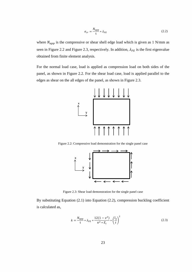
23

𝜎𝑐𝑟 =𝑁𝑎𝑝𝑝

t∗ 𝜆𝐹𝐸 (2.2)

where 𝑁𝑎𝑝𝑝 is the compressive or shear shell edge load which is given as 1 N/mm as

seen in Figure 2.2 and Figure 2.3, respectively. In addition, 𝜆𝐹𝐸 is the first eigenvalue

obtained from finite element analysis.

For the normal load case, load is applied as compression load on both sides of the

panel, as shown in Figure 2.2. For the shear load case, load is applied parallel to the

edges as shear on the all edges of the panel, as shown in Figure 2.3.

Figure 2.2: Compressive load demonstration for the single panel case

Figure 2.3: Shear load demonstration for the single panel case

By substituting Equation (2.1) into Equation (2.2), compression buckling coefficient

is calculated as,

𝑘 =𝑁𝑎𝑝𝑝

t∗ 𝜆𝐹𝐸 ∗

12(1 − 𝑣2)

𝜋2 ∗ 𝐸𝑐∗ (𝑙𝑦

𝑡)

2

(2.3)

24

To construct the finite element model, ABAQUS, is used in the analyses of unstiffened

panel models [35]. As in all commercial FEA programs, the modelling process starts

with creating the geometry, then with meshing is performed and material properties

are assigned to the unstiffened panel. The modelling process finishes by defining load

and boundary conditions. Scope of the study is limited to flat thin panels under

unidirectional compression and shear loads which are applied separately. Loads are

given as edge unit load and boundary conditions are used as described in Table 2.1 and

Table 2.2. Thin panel is modelled as a shell structure in the FE model as seen in Figure

2.4. In the meshing part, S4R elements (4-node element with one integration point),

with hourglass control and membrane strain is chosen. This type element is

recommended by ABAQUS in modelling of shell structures [35]. For the unstiffened

panel models, “Buckle” step of ABAQUS [35] is used to obtain the lowest buckling

eigenvalue. Subspace solver is chosen in order to avoid divergence problem. In the

Subspace solver, there are 3 input parameters can be defined by users in the ABAQUS.

These are the number of intended eigenvalues, vectors used per iteration and maximum

number of iteration. In this study, three eigenvalues, ten vectors used per iteration and

3000 maximum number of iterations are chosen to avoid divergence. These values are

recommended by the ABAQUS manuel for the buckling analysis [35].

Figure 2.4: View of sample single panel model with all edges simply supported under compressive

loading

25

Before the verification of finite element model’s boundary conditions, element sizes

used in the rest of study is determined by the mesh convergence study. To get fast and

accurate result, nine different mesh sizes is chosen (course mesh, fine mesh and regular

mesh). In the convergence study, example panel dimensions are chosen as 100 mm

length x and 200 mm length y. Thickness of panel is decided as 1 mm. Material of the

panel is also decided as Aluminum 2024 T3 Clad sheet [36]. Detailed material

properties can be seen in Appendix B, Figure B.1. Boundary condition of the panel is

chosen as simply supported boundary condition defined in Table 2.1 and load is given

as unit shell edge load in the x direction along the edges AB and DC shown in Figure

2.1. Figure 2.5 shows the critical buckling stress with respect to element number used

in the finite element mesh in the panel. In addition, element sizes used in this

convergence study and the corresponding critical buckling stress results are given in

Table 2.5. As seen in Table 2.5, as the element size is decreased, the critical buckling

stress converges to approximately 27.1 MPa. After the element size become 5 mm and

less, critical buckling stress does not significantly change. Hence, to minimize the

computation time and not to lose accuracy, element size is taken as 5 mm.

Figure 2.5: The critical buckling stress with respect to element number of flat panel

26.9

27.1

27.3

27.5

27.7

0.00E+00 1.00E+04 2.00E+04

Cri

tica

l Bu

cklin

g St

ress

(M

Pa)

Number of Element

26

Table 2.5: Critical buckling stress results for various element sizes

Element Size (mm) Number of Elements Critical Buckling Stress (MPa)

1 20000 27.068

2 5000 27.112

3 2211 27.162

4 1250 27.212

5 800 27.267

6 561 27.321

7 406 27.405

8 325 27.448

9 242 27.563

10 200 27.648

After the convergence study, to compare the finite element analysis results for the

compression buckling coefficient with those provided by Bruhn [1], figures of

buckling coefficients given by Bruhn are digitized to compare with the FEA results.

Interval of the panel length x is chosen as the 100 mm to 500 mm with 5 mm step size.

In addition, panel length y is chosen as constant 100 mm and the panel thickness is

decided as constant 2 mm.

Comparison of buckling coefficient versus plate aspect ratio curves are given in Figure

2.6-Figure 2.9, for different loading and boundary conditions.

27

Figure 2.6: Comparison of compressive buckling charts for flat rectangular panels with simply

supported loaded and unloaded edges

Figure 2.7: Comparison of compressive buckling charts for flat rectangular panels with clamped

loaded and unloaded edges

28

Figure 2.8: Comparison of shear buckling charts for flat rectangular panels with simple supported

loaded and unloaded edges

Figure 2.9: Comparison of shear buckling charts for flat rectangular panels with clamped loaded and

unloaded edges

It should be noted that average of the differences between the buckling coefficients

obtained by the finite element analysis and analytically determined buckling

coefficients provided by Bruhn are around %1-2 in Figure 2.6-Figure 2.9. It is also

noted that differences are mainly due to digitizing the plots given by Bruhn [1].

29

2.2. Buckling Analysis of Stiffened Panels

2.2.1. Determination of buckling coefficients of skin-stringer assemblies by finite

element analysis

Following the verification of the boundary conditions of a single panel by the finite

element analysis, stiffened panel modelling is performed using the verified boundary

conditions along the loaded edges of the panel. However, for the stiffened panels,

restraint along the unloaded edges is provided by the stiffeners on the panel. The

boundary condition of the loaded edges of skin-stringer assembly is considered as

clamped edge condition.

The first skin-stringer assembly considered consists of three flat skin panels and two

stringers with I cross section. Skin-stringer assembly and the skin panel numbering are

demonstrated in Figure 2.10.In addition, cross section view of skin-stringer assembly

is seen in Figure 2.12. Compression load is applied on the three skin panels from one

of the edges along the y-axis as 1 N/mm edge load in the -x direction. Figure 2.11

demonstrates the restraints applied to the loaded and the opposite edges of the panel.

The degrees of freedom restrained along the loaded edge are U3 and R2. Along the

other edge of the three skin panels, degrees of freedom U1, U3 and R2 are restrained.

In addition, the middle edge of panel 2 is not allowed move in the y direction to avoid

rigid body motion of the assembly, as shown in Figure 2.11. Moreover, unloaded side

edges of the panels 1 and 3 are restrained in z-translation (U3 degree of freedom) and

x-rotation (R1 degree of freedom).

30

Figure 2.10: Isometric view of skin-stringer assembly analyzed

Figure 2.11: Constraint configuration of the skin-stringer assembly

31

Figure 2.12: Cross section view of skin-stringer assembly analyzed

In the finite element model of the skin-stringer assembly, all stringers and skin panels

are modelled as 2D shell elements with Aluminum 2024 T3 sheet material properties

as shown in Figure 2.13 same as the unstiffened panel model. Element type used is

shell element, S4R type which is a 4-node element with one integration point. Material

properties of Aluminum 2024 T3 sheet is given in Table 2.3 [36]. Stringers element

size is chosen as 2 mm and skin element size is chosen as 5 mm same as the unstiffened

panel model. Stringer mesh density is chosen higher than skin mesh density because

the dimension of stringer cross section is smaller than skin dimensions. Stringers are

connected to the skins by 3.2 mm diameter fasteners in double row arrangement.

Fastener spacing is taken as 5 times the fastener diameter and fastener edge distance

is the 2 times the fastener diameter plus 1 mm as shown in Figure 2.14. These figures

are commonly used in the aerospace industry.

Figure 2.13: Isometric view of skin-stringer assembly with mesh

32

Since it is too costly to model each fastener using its real geometry with a 3D model,

fastener idealization is made. For this purpose, mesh-independent fastener is

considered as a convenient method to define a point-to-point connection between two

or more surfaces such as in a fastener connection. Thus, in the finite element model of

the skin-stringer assembly, fasteners are modelled with the mesh-independent fastener

module in ABAQUS [35].

Figure 2.14: Fastener pattern configuration on the stringer

For the skin-stringer assembly, “Buckle” step of ABAQUS is used to obtain the lowest

buckling eigenvalue [35]. Lowest eigenvalue obtained by finite element analysis is

used in Equation (2.3) to calculate the compression buckling coefficient pertaining to

the local buckling of the skin supported by the side stiffeners.

A case study is performed for a panel with the loaded edges which are considered as

clamped edge conditions and the unloaded edges closely simulating the clamped edge

conditions with the help of stringer stiffness. Compression buckling coefficients

calculated by the finite element solution are compared with the analytically determined

compression buckling coefficient for panel 2 (mid panel) in the skin-stringer assembly

as shown in Figure 2.10. Input parameters of this example assembly are shown in Table

2.6. The parameters given in Table 2.6 are decided iteratively such that with these

parameters the unloaded edges simulate the clamped condition closely. The skin-

33

stringer model is solved by using “Buckle” step of ABAQUS for the lowest buckling

eigenvalue as described previously [35].

Table 2.6: Input parameters of the skin-stringer assembly used in the finite element model

Skin panel material Aluminum 2024 T3 Clad Sheet


Skin panel length x (mm) 450.0

Skin panel length y (mm) 150.0

Stringer material Aluminum 2024 T3 Clad Sheet

Stringer thickness (mm) 1.016

Stringer height (mm) 14.0

Stringer upper flange width (mm) 9.0

Stringer lower flange width (mm) 11.5

𝑁𝑎𝑝𝑝 is compressive shell edge load applied on the three skin panels from one of the

edges along the y-axis which is given as 1 N/mm in the -x direction. For the skin-

stringer assembly specified in Table 2.6, the lowest eigenvalue is obtained as,

𝜆𝐹𝐸 = 12.006 (2.4)

Using this eigenvalue, the corresponding compressive stress and the compressive

buckling coefficient are calculated as,

𝜎𝑐𝑟 = 14.768 𝑁/𝑚𝑚2 (2.5)

𝑘 = 7.383 (2.6)

If the skin panel 2 in Figure 2.10 is modeled with the same input parameters but

classical clamped edge condition is assigned to the unloaded edges, for the panel aspect

ratio of 3, compressive buckling coefficient is obtained as:

34

𝑘 = 7.382 (2.7)

In this example, it is seen that for the skin-stringer assembly defined in Table 2.6, the

unloaded edge of panel 2 closely simulates the clamped edge condition. However,

depending on the stringer type and how the stringer is connected to the skin, buckling

coefficients obtained from the finite element analysis may or may not agree with the

buckling coefficients obtained from pure analytical study utilizing the classical

boundary conditions.

According to the model description made, a script is written Python 2.7 in order to

create an ABAQUS finite element model, run the model and collect the lowest

eigenvalue from the analysis results. The purpose of this process is the preparing

databases for the buckling coefficients of selected metallic skin-stringer assemblies by

means of parametric modelling approach via the script language. With this approach,

databases of buckling coefficients for skin-stringer assemblies can to be generated

similar to the available buckling coefficient charts for the panels which have classical

boundary conditions along the edges.

In this chapter, most commonly used stringer sections Z, J and T are investigated.

Stringer section types’ geometric descriptions are shown in Figure 2.15. As seen in

Figure 2.15, T and J stringer section types use the double row joint configuration at

the connection of skin and the lower flange of the stringer. In contrast, in the Z type

stringer section, the single row joint configuration is used the finite element models.

The scripts are written for each skin-stringer assembly and the following parameters

are specified;

• Skin panel thickness

• Skin panel length y

• Stringer thickness

• Stinger height

35

• Stringer lower flange length

• Stringer upper flange length (In stringer section type T, there is no upper

flange)

Figure 2.15: Stringer section types used in skin-stringer assemblies

To minimize the time and sources, some of the parameters of the skin-stringer

assemblies are fixed to certain values as,

• Skin panel length x = 450 mm

• Fastener diameter = 3.2 mm

• Material: Aluminum 2024 T3 Clad Sheet

Discrete values of the design parameters of the skin-stringer assemblies are specified

in a range. Upper and lower limits of the design parameters are decided based on the

commonly used values in the industry.

For the skin-stringer assemblies with Z and J type stringers, the following parameters

are specified between the upper and lower limits, and in total 2160 finite element

analyses are performed to form a database for the buckling coefficients.

• Skin panel thickness = [0.813, 1.016, 1.27] mm

• Skin panel length y = [150.0, 225.0, 300.0, 375.0, 450.0] mm

36

• Stringer thickness = [0.813, 1.016, 1.27] mm

• Stinger height = [10.0, 17.0, 24.0, 30.0] mm

• Stringer lower flange length = [10.0, 14.0, 18.0, 22.0] mm

• Stringer upper flange length = [10.0, 14.0, 18.0] mm

For the skin-stringer assembly with the T section stringer, the following parameters

are specified between the upper and lower limits, and in total 2100 finite element

analyses are performed to form a database for the buckling coefficients.

• Skin panel thickness = [0.813, 1.016, 1.10, 1.27] mm

• Skin panel length y = [150.0, 225.0, 300.0, 375.0, 450.0] mm

• Stringer thickness = [0.813, 1.016, 1.10, 1.27] mm

• Stinger height = [10.0, 15.0, 20.0, 25.0, 30.0] mm

• Stringer lower flange length = [10.0, 13.0, 16.0, 19.0, 22.0] mm

To minimize the number of finite element analysis, for each parameter minimum

number of discrete values are selected within the upper-lower limits of each parameter.

Skin length y has a remarkable effect on the buckling phenomena. Hence, for the skin

length y, more number of discrete analysis points is used in the finite element analyses.

However, for Z and J stringer section types, inner flange length is restricted to three

values in order to minimize the number of analyses.

37

2.2.2. Setting up of Artifitial Neural Network and Response Surface for fast

determination of buckling coefficients

For fast determination of the buckling coefficients of skin-stringer assemblies with

different stringer types, in this chapter, artificial neural network and response surface

are set up utilizing the finite element analysis results for the buckling coefficients. The

output parameter, buckling coefficient, obtained from finite element analyses and input

parameters of the skin-stringer assemblies are collected in an Excel file for the

generation of the ANN and the RS for fast and accurate determination of buckling

coefficients without resorting to finite element analysis. For the generation of the

response surface, inputs and outputs are processed in MATLAB RSTOOL [37].

Response surface model is chosen as “Full Quadratic”. Full quadratic response surface

consists of constant term, the linear terms, the interaction terms and the squared terms.

As the second fast and accurate analysis tool, an artificial neural network is chosen.

Artificial neural networks (ANNs) are computational modeling tools to model linear

and nonlinear complex systems with most traditional statistical approaches. ANNs

have characteristic advantages such as being suitable for nonlinear problems and

ANNs have parallel working ability. Furthermore, ANNs can process imprecise and

fuzzy information. Thus, they can provide accurate solutions for uncertain data. These

capabilities deliver important benefits of excellent data fitting, adaptability and

modeling of unlearned data [38].

ANN consists of multiple numbers of individual artificial neurons. These individual

artificial neurons are grouped to create a layer in an artificial neural network. Neurons

of each layer are connected to the neurons of the next layer. The ANN is composed of

three layers which are input layer, hidden layer and output layer. The number of

neurons in the input and the output layers are determined by the number of the input

and the output parameters. Each neuron is associated with one input or output

parameter. Thus, computational ability of an ANN is determined by the number and

the content of hidden layers [37, 38]. Number of neurons in hidden layers is determined

by trial and error to adjust the ANN with desired capabilities. Example of an artificial

neural network configuration is shown in Figure 2.16. In this configuration, three

38

neurons input layer that is used to take three input parameters to the system, one neuron

output layer that returns an output as result of the computation process, and two

neurons for hidden layers.

Figure 2.16: Configuration of artificial neural network

In this study, an artificial neural network is established for each skin-stringer assembly

by using the input parameters and the output parameter which is the buckling

coefficient. Buckling coefficients are in the range of 6-8 for the skin-stringer

assemblies with J, Z and T type stringers. Inputs and output of numerous analyses are

processed in MATLAB NNTOOL to create an artificial neural network (ANN) [24,

37, 38]. In the ANN, total layer number is chosen as 2, one for output layer and the

other one for hidden layer. Number of neuron number in the ANN is decided by trial

and error method for each type of stringer section. Levenberg-Marquardt

backpropagation is chosen for training method of ANN. One of the termination criteria

of neural network training process are decided as maximum “mu” which is known as

the momentum term to slow the speed of the descent so that the search value does not

fly back and forth across the minimum without stopping sufficiently near it. Another

termination criterion is the minimum performance gradient which is gradient of the

square of the error function with respect to the unknown weights and biases. As the

39

third and fourth termination criteria, maximum number of iteration, which is the

number of iterations without any improvement and the epoch limit which is defined as

the limit of the iteration number are used. In this study, these criteria are chosen as

1e10 for maximum “mu”, 1e-7 for minimum performance gradient, 500 for maximum

number of iteration without any improvement and 1500 for epoch limit. For each type

of stringer section, different ANN parameters are chosen to obtain accurate results.

These parameters are neuron number, percentage of data sets used in the training set,

percentage of data sets used in the validation set and percentage of data sets used in

the test set. According to these parameters, performance of network is measured based

on the mean squared error calculated using difference of ANN and FEA results.

The best network performance is obtained for the skin-stringer assembly with J type

stringer section for the following set of parameters:

• 1 Neuron number

• % 70 of the data set used in the training of the ANN

• % 15 of the data set used in the validation of the ANN

• % 15 of the data set used in the test of the ANN

Using these parameters in ANN, for the skin-stringer assemblies with J type stringer

section, mean square error is calculated as 5.12 ∗ 10−4 as seen in Figure 2.17.

40

Figure 2.17: Performance plot of the ANN for skin-J type stringer assembly

The best network performance is obtained for Z type stringer section for the following

set of parameters:

• 10 Neuron number

• % 70 of the data set used in the training of the ANN

• % 15 of the data set used in the validation of the ANN

• % 15 of the data set used in the test of the ANN

Using these parameters in ANN, for the skin-stringer assemblies with Z type stringer


41

Figure 2.18: Performance plot of the ANN for skin-Z type stringer assembly

The best network performance is obtained for T type stinger section for the following

set of parameters:

• 10 Neuron number

• % 75 of data set used in the training of the ANN

• % 15 of data set used in the validation of the ANN

• % 10 of data set used in the test of the ANN

Using these parameters in the ANN, for skin-stringer assemblies with T type stringer


42

Figure 2.19: Performance plot of the ANN for skin-T type stringer assembly

ANN performance can also be shown with the regression lines given in Figure 2.20,

Figure 2.21 and Figure 2.22 for the J, Z and T type of stringers, respectively. In the

plots, vertical axis shows the ANN outputs which are obtained by using input database

and the horizontal axis shows the FEA results that are used in training of the ANN.

The dashed lines in the figures represent the perfect fit and the colorful lines are the

fits that are created by training process. It is seen that colorful lines are very close to

the dashed lines in each figures.

43

Figure 2.20: Overall, training, validation and testing regression plots of the ANN for skin-J type

stringer assembly

44

Figure 2.21: Overall, training, validation and testing regression plots of the ANN for skin-Z type

stringer assembly

45

Figure 2.22: Overall, training, validation and testing regression plots of the ANN for skin-T type

stringer assembly

In addition, Figure 2.23, Figure 2.24 and Figure 2.25 show the cause for termination

of the training for the skin-stringer assemblies with J, Z and T type of stringers,

respectively. It is seen that the ANN performance for the skin-stringer assemblies with

J type of stringer does not increase after 254 iteration as shown in Figure 2.23. Thus,

the validation fails 500th times at the iteration 754. As seen in the Figure 2.23, gradient

of ANN for the skin-stringer assemblies with J type of stringer is obtained as 2.436e-

5 which is higher than minimum gradient value. In addition, “mu” value of this ANN

is obtained as 1e-7 which is lower than maximum “mu” value at the iteration 754. For

46

skin-stringer assembly with Z type of stringer, the ANN performance does not increase

after 458 iteration as seen in Figure 2.24. Moreover, for skin-stringer assembly with T

type of stringer, the ANN performance does not increase after 977 iteration as seen in

Figure 2.25.

Figure 2.23: Number of validation fails, mu and gradient with respect to number of training iterations

of ANN for skin-J type stringer assembly

47


of ANN for skin-Z type stringer assembly

48


of ANN for skin-T type stringer assembly

49

2.2.3. Comparison of buckling coefficients of skin-stringer assemblies

determined by FEA, Response Surface and Artificial Network

2.2.3.1. BUCKLING COEFFICIENTS OF SKIN-STRINGER ASSEMBLIES WITH J

TYPE STRINGERS

Table 2.7 shows the input parameters of 10 additional analyses for the determination

of buckling coefficients of skin-stringer assemblies. Parameters given in Table 2.7 are

selected in between the parameters used in the finite element analyses used for the

setup of the finite element database. Table 2.8 gives the finite element analysis (FEA),

response surface (RS) and the artificial neural network (ANN) results.

Table 2.7: FEA input parameters for additional analyses for skin-stringer assemblies with ‘J' type

stringer

FEA 1 2 3 4 5 6 7 8 9 10

Skin panel

thickness

(mm)

1.05 0.85 1.2 1.2 1.15 1.05 1 0.9 1.1 1.15

Skin panel

length x

(mm)

450 450 450 450 450 450 450 450 450 450

Skin panel

length y

(mm)

350 200 325 320 400 275 200 175 235 325

Stringer

thickness

(mm)

1.1 1 1.2 1.25 1.2 1.07 1.03 1 1.15 1.2

Stringer

height (mm) 18 13 28 25.5 17.5 16 19 18 22 23

Stringer

upper

flange width

(mm)

15 12 17 16 15.5 11 13.5 10.5 15.5 16.5

Stringer

lower flange

width (mm)

16.5 15 17.5 17 15.5 12.5 14.75 11 15.75 17.75

50

Table 2.8: Buckling coefficients of skin-stringer assemblies with J type stringers / FEA results/ RS

results / ANN results

# FEA

Results

RS

Results

% Absolute

Difference (RS)

ANN

Results

% Absolute

Difference (ANN)

1 7.83 7.963 1.69 7.842 0.15

2 7.59 7.628 0.51 7.559 0.41

3 8.08 7.958 1.50 8.049 0.39

4 8.07 7.959 1.37 8.058 0.15

5 7.9 8.118 2.76 7.901 0.02

6 7.27 7.330 0.83 7.394 1.70

7 7.47 7.489 0.25 7.444 0.34

8 7.26 7.320 0.82 7.326 0.91

9 7.52 7.675 2.06 7.517 0.04

10 7.88 7.994 1.45 8.068 2.38

For the skin-stringer assembly with J type stringer, Table 2.8 shows that the established

ANN performs better than the RS. For the randomly selected 10 set of design

parameters, root mean square (RMS) error with respect to the finite element results is

0.0760 for the ANN and 0.1176 for the RS.

51

2.2.3.2. BUCKLING COEFFICIENTS OF SKIN-STRINGER ASSEMBLIES WITH Z

TYPE STRINGERS


of buckling coefficients of skin-stringer assemblies. Parameters given in Table 2.9 are

selected in between the parameters used in the finite element used for the setup of the

finite element database. Table 2.10 gives the finite element analysis (FEA), response

surface (RS) and the artificial neural network (ANN) results.

Table 2.9: FEA input parameters for additional analyses for skin-stringer assemblies with ‘Z' type

stringer

FEA 1 2 3 4 5 6 7 8 9 10

Skin panel

thickness

(mm)

1.05 0.85 1.2 1.2 1.15 1.05 1 0.9 1.1 1.15

Skin panel

length x

(mm)

450 450 450 450 450 450 450 450 450 450

Skin panel

length y

(mm)

350 200 325 320 400 275 200 175 235 325

Stringer

thickness

(mm)

1.1 1 1.2 1.25 1.2 1.07 1.03 1 1.15 1.2

Stringer

height (mm) 18 13 28 25.5 17.5 16 19 18 22 23

Stringer

upper

flange width

(mm)

15 12 17 16 15.5 11 13.5 10.5 15.5 16.5

Stringer

lower flange

width (mm)

16.5 15 17.5 17 15.5 12.5 14.75 11 15.75 17.75

52

Table 2.10: Buckling coefficients of skin-stringer assemblies with Z type stringers / FEA results/ RS


# FEA

Results

RS

Results

% Absolute

Difference (RS)

ANN

Results

% Absolute

Difference (ANN)

1 7.46 7.601 1.88 7.475 0.20

2 7.01 7.096 1.23 7.014 0.06

3 7.63 7.547 1.09 7.593 0.49

4 7.64 7.552 1.15 7.612 0.37

5 7.61 7.812 2.66 7.593 0.22

6 6.98 7.019 0.55 7.108 1.83

7 6.92 6.958 0.55 6.888 0.46

8 6.83 6.918 1.29 6.932 1.50

9 6.97 7.174 2.93 6.919 0.74

10 7.46 7.575 1.54 7.600 1.88

For the skin-stringer assembly with Z type stringer, Table 2.10 shows that the

established ANN performs better than the RS. For the randomly selected 10 set of

design parameters, root mean square (RMS) error with respect to the finite element

results is 0.0726 for the ANN and 0.1219 for the RS.

53

2.2.3.3. BUCKLING COEFFICIENTS OF SKIN-STRINGER ASSEMBLIES WITH T

TYPE STRINGERS


of buckling coefficients of skin-stringer assemblies. Parameters given in Table 2.11

are selected in between the parameters used in the finite element analyses used for the

setup of the finite element database. Table 2.12 gives the finite element analysis (FEA),

response surface (RS) and the artificial neural network (ANN) results.

Table 2.11: FEA input parameters for additional analyses for skin-stringer assemblies with ‘T' type

stringer

FEA 1 2 3 4 5 6 7 8 9 10

Skin panel

thickness

(mm)

1.05 0.85 1.2 1.2 1.15 1.05 1 0.9 1.1 1.15

Skin panel

length x

(mm)

450 450 450 450 450 450 450 450 450 450

Skin panel

length y

(mm)

350 200 325 320 400 275 200 175 235 325

Stringer

thickness

(mm)

1.1 1 1.2 1.25 1.2 1.07 1.03 1 1.15 1.2

Stringer

height (mm) 18 13 28 25.5 17.5 16 19 18 22 23

Stringer

lower flange

width (mm)

16.5 15 17.5 17 15.5 12.5 14.75 11 15.75 17.75

54

Table 2.12: Buckling coefficients of skin-stringer assemblies with T type stringers / FEA results/ RS


# FEA

Results

RS

Results

% Absolute

Difference (RS)

ANN

Results

% Absolute

Difference (ANN)

1 7.39 7.591 2.73 7.300 1.22

2 6.91 6.932 0.32 6.878 0.46

3 7.46 7.575 1.55 7.475 0.20

4 7.49 7.604 1.52 7.500 0.13

5 7.55 7.805 3.37 7.619 0.91

6 6.9 6.863 0.53 7.020 1.74

7 6.71 6.893 2.73 6.697 0.19

8 6.56 6.758 3.02 6.569 0.14

9 6.82 7.164 5.04 6.824 0.06

10 7.36 7.614 3.45 7.337 0.32

For the skin-stringer assembly with T type stringer, Table 2.12 shows that the

established ANN performs better than the RS. For the randomly selected 10 set of

design parameters, root mean square (RMS) error with respect to the finite element

results is 0.0542 for the ANN and 0.1972 for the RS.

55

2.2.3.4. DISCUSSION OF RESULTS OBTAINED BY FEA, ANN AND RS FOR J, Z

AND T TYPE OF STRINGER

In these additional 10 analyses, it is seen that for the skin-stringer assemblies defined

in Table 2.7, Table 2.9 and Table 2.11 for ‘J’, ‘Z’ and ‘T’ type of stringer sections,

absolute difference between RS results and FEA results is not greater than 5%. RS

gives fast convergence but this method does not give accurate results as the ANN.

Absolute difference between the ANN results and FEA results is not greater than 2.5%.

However, ANN also has a problem with convergence. If the neuron number is

increased too much, for instance over 10 for the buckling problem, over fitting occurs.

It should be noted that when over fitting occurs, error of the training set is driven to a

very small value, but for the new data in between the data points used to generate the

database, the error is large. Moreover, to get an accurate ANN result, many data sets

are required. For the determination of the buckling coefficients, at least 2000 data sets

are required to obtain reasonable results which are close to the finite element results

with acceptable difference. Nevertheless, the established ANN can be used very

effectively to determine the buckling coefficients of skin-stringer assemblies with

common J, Z and T type stiffeners. If desired ANN can be utilized to construct

buckling coefficients charts similar to the buckling coefficient charts available for

panel buckling with classical boundary conditions.

56

57

CHAPTER 3

3. POST BUCKLING LOAD DISTRIBUTION OF METAL STIFFENED

PANELS

In this chapter, post buckling load distribution and the effect of material nonlinearity

on the load redistribution in the post-buckled stage is investigated using linear and

nonlinear material models with different stringer types of skin-stringer assemblies by

ABAQUS finite element analysis. For this purpose, in the first part of the study, a

baseline stiffened panel is generated for further investigation of the material

nonlinearity on the post-buckling behavior and on the effective width of the stiffened

panel. To make a direct comparison with the classical approach for the determination

of the effective width of the skin panel, a stiffener section which provides classical

clamped edge condition is designed such that the compression buckling coefficient

determined by the finite element analysis agreed closely with the analytically

determined buckling coefficient of the clamped edge panel.

In the second part of the chapter, post-buckling analysis of the stiffened panel is

performed utilizing linear and nonlinear material models with three different stringer

types (I, J and Z) in the finite element analysis and the effect of material plasticity on

the post-buckling behavior of the panel is studied. The effective width of the panel is

calculated before the collapse load of the panel using the load distributions obtained

by finite element analysis with linear and nonlinear material models and comparisons

58

are with the effective width calculated using the classical effective width formulation.

At the end of the chapter, finite element model analysis results are obtained for

combination of each stringer types and material models. Its means that totally 6 finite

element model is created and effective width results are compared to each other.

3.1. Buckling Analysis of the Baseline Skin-Stringer Assembly

Baseline stiffened panel is designed in an iterative fashion to decide on the dimensions

of the side stiffeners such that side stiffeners provided nearly clamped edge condition.

For this purpose, compressive buckling coefficient of the stiffened flat panel is

calculated by the finite element analysis until a close agreement is reached with the

determined compressive buckling coefficient by the finite element analysis of clamped

edge unstiffened panel.

Before the decision of the proper stiffener cross-section, buckling analysis of the flat

panel with the classical clamped edge conditions is performed and the compression

buckling coefficient is also obtained via finite element analysis before the addition of

the side stiffeners. As previously defined in Figure 2.1, the geometry and the

coordinate system of the panel is used in the construction of the unstiffened panel.

Boundary condition of the unstiffened panel is defined as all edges clamped defined

in Table 2.2.

However, in this case, load is applied from the DC edge along the y-axis of the single

panel as 2.0 mm displacement in the “-x” direction (compression) and the reaction

edge of the panel is taken as AB edge. Thus, in this case, in addition to boundary

conditions defined in Table 2.2, AB edge is also restricted in translational degree of

freedom in the x direction. Although, this additional boundary condition has no effect

on the buckling coefficient result, it is necessary to fix the edge AB in order to be able

to read reaction forces from the nodes along the edge AB in post-buckling analyses

presented in this chapter.

After the determination of the boundary condition and the input displacement, input

parameters of the unstiffened skin panel studied are decided as given in Table 3.1. The

59

unstiffened panel model without any side stiffeners is solved by using “Buckle” step

of ABAQUS in linear buckling analysis for the lowest buckling eigenvalue [35].

Table 3.1: Input parameters of the unstiffened skin panel used to verify stiffened panel edge condition

Skin panel material Aluminum 2024 T3 Sheet


Skin panel length x (mm) 450

Skin panel length y (mm) 150

For the unstiffened panel model described in Table 3.1, lowest eigenvalue is obtained

as,

𝜆𝐹𝐸 = 0.0450 (3.1)


buckling coefficient are calculated as,

𝑢𝑐𝑟 = 𝑢𝐹𝐸 ∗ 𝜆𝐹𝐸 = 0.090 𝑚𝑚 (3.2)

𝜎𝑐𝑟 =𝑢𝑐𝑟𝑙𝑥𝐸𝑐 = 14.77 𝑀𝑃𝑎 (3.3)

𝑘 = 𝜎𝑐𝑟12(1 − 𝑣2)

𝜋2𝐸𝑐(𝑙𝑦

𝑡)

2

= 7.38 (3.4)

After calculation of the buckling coefficient of the unstiffened panel with all edges

clamped boundary conditions by the finite element analysis, stiffened panel modeling

is performed using the clamped boundary conditions along the loaded edges of the

panel. For the stiffened panels, side stiffeners provide constraint along the unloaded

edges of the panel. To generate the clamped edge condition along the unloaded edges

of the stiffened panel, an iterative procedure is used to decide on the dimensions of the

stiffener. To study the post-buckling behavior of the stiffened panel, the considered

skin-stringer assembly consists of three flat skin panels and two stringers with I cross

section. Mesh-independent fasteners available in ABAQUS are used in the skin-

60

stringer connection [35]. Skin-stringer assembly and the skin panel numbering are

demonstrated in Figure 3.1. For the skin-stringer assembly, a compression load is

applied in the -x direction as prescribed displacement on one of the edges along the y-

direction.

Figure 3.1: Baseline skin-stringer assembly

Figure 3.2 shows the restraints applied to the loaded and the opposite edges of the skin-

stringer assembly. To simulate the clamped edge condition, the degrees of freedom

restrained along the loaded edges are U3 (z-direction displacement) and R2 (rotation

about the y-axis). Along the opposite edge of the loading edge of the skin-stringer

assembly, degrees of freedom U1, U3 and R2 are restrained. In addition, the mid-point

of panel 2 is not allowed move in the y-direction to avoid rigid body motion of the

assembly, as shown in Figure 3.2. Moreover, unloaded side edges of the panels 1 and

3 are restrained in z-translation (U3 degree of freedom) and x-rotation (R1 degree of

freedom).

61

Figure 3.2: Constraints applied to the baseline skin-stringer assembly

In the finite element model of the baseline skin-stringer assembly, all stringers and

skin panels are modeled as 2D shell elements with Aluminum 2024 T3 sheet material

properties [36]. Same fastener configurations and modelling technics written in

chapter 2.2 are used in the finite element model of baseline skin-stringer assembly.

Fastener configurations used in baseline skin-stringer assembly is shown in Figure

2.14.

For the skin-stringer assembly, “Buckle” step of ABAQUS is used in linear buckling

analysis to obtain the lowest buckling eigenvalue [35]. The lowest buckling eigenvalue

is used in Equation (3.4) to calculate the compression buckling coefficient pertaining

to the local buckling of the skin supported by the side stiffeners. By comparing the

compression buckling coefficient calculated by the finite element solution with the

determined compression buckling coefficient by finite element model of unstiffened

panel defined in Table 3.1, clamped edge condition provided by the side stiffeners is

verified.

Stringer dimensions are changed until the compression buckling coefficient obtained

by the finite element analysis agreed closely with the finite element result of 7.38 given

62

by Equation (3.1). For this purpose, parametric modeling of the skin-stringer assembly

is performed via the script language followed by automated finite element analysis by

ABAQUS [35]. I type of stringer dimensions which simulate the clamped edge

boundary condition closely are given in Table 3.2 together with the overall dimensions

of the skin-stringer assembly.

For the buckling analysis, a compression load is applied on one of the edges of the

skin-stringer assembly with the I type of stringer section along the y-axis as 2.0 mm

prescribed displacement in the “-x” direction. For the skin-stringer assembly described

in Table 3.2, lowest eigenvalue is obtained as,

𝜆𝐹𝐸 = 0.0450 (3.5)

Table 3.2: Parameters of the skin-stringer assembly used in the finite element model with I section

stringer




Single skin panel length y (mm) 150

Stringer material Aluminum 2024 T3 Sheet


Stringer height (mm) 25

Stringer upper flange width (mm) 15

Stringer lower flange width (mm) 20


buckling coefficient of skin-stringer assembly with I stringer section type are

calculated as,

𝑢𝑐𝑟 = 𝑢𝐹𝐸 ∗ 𝜆𝐹𝐸 = 0.090 𝑚𝑚 (3.6)

63

𝜎𝑐𝑟 =𝑢𝑐𝑟𝑙𝑥𝐸𝑐 = 14.77 𝑀𝑃𝑎 (3.7)

𝑘 = 𝜎𝑐𝑟12(1 − 𝑣2)


𝑡)

2

= 7.38 (3.8)

Comparing the results given by Equation (3.4) and Equation (3.8), it is concluded that

the properties of the I section stringer given in Table 3.2 provides the clamped edge

condition along the unloaded edges of the skin-stringer assembly.

3.2. Post-Buckling Analysis of Skin-Stringer Assembly using Linear and Non-

linear Material Models

Following the verification of the compression buckling coefficient of the stiffened

panel with finite element model, the post-buckling behavior of the skin-stringer

assembly is investigated with two different models; with linear and nonlinear material

models. In both models, “Non-linear Geometric Static Analysis” step of ABAQUS is

used to observe the post-buckling behavior of the stiffened panel [35]. For both

models, load carrying capacity of the assembly and the effective width of the skin

panel are calculated using the finite element results. Moreover, effective width

calculation is also done utilizing the empirical relation following Bruhn [1].

For the analysis of the post-buckling load distribution, nodal forces in the x-direction

of the restrained edge of the skin panel are summed up to calculate load capacity of

assembly. Additionally, one of the nodes in the loaded edge is used to trace the

displacement of skin-stringer assembly. Restrained and loaded edges are shown in

Figure 3.3 with red and green lines, respectively.

64

Figure 3.3: Edge descriptions of the skin-stringer assembly

To investigate the post-buckling behavior of the skin-stringer assembly, geometrically

nonlinear analysis of the skin-stringer assembly with I section stringer is conducted by

the “Non-linear Static Analysis” step of ABAQUS [35]. As in the previous analyses,

a compression load is applied on one of the edges of the skin-stringer assembly along

the y-axis as 2.0 mm prescribed displacement in the “-x” direction. Material and

geometric description of the previous assembly which is used for verification of the

clamped edge condition in chapter 3.1, is used for the both material models created in

this chapter. In addition to the linear material model, nonlinear stress-strain data given

in Appendix B is used in the ABAQUS material description. Defining material

plasticity in ABAQUS is presented in the research report by Rasmussen [39]. Material

properties of the aluminum 2024-T3 sheet are given in Figure B.1 [36]. For aluminum

2024-T3, stress-strain curve including the plastic region is given in Figure B.2. For the

nonlinear material model, the stress-strain data given in Table B.1 is used in the post-

buckling analysis.

Firstly, using the linear material model for the skin-stringer assembly, load-

displacement curve is obtained by ABAQUS analysis as shown in Figure 3.4.

65

Figure 3.4: Load displacement curve of the skin-stringer assembly with linear material model (I

section stringer)

As shown in Figure 3.4, the first break in the load-displacement curve represents the

initiation of the local buckling. Local buckling starts when the applied displacement is

0.107 mm. This result is different than the critical displacement determined in linear

buckling analysis (𝑢𝑐𝑟 = 0.090 𝑚𝑚). The reason of this difference is attributed to

including the geometric non-linearity in the post-buckling model. Beyond the

initiation of the local buckling, post-buckling stage of the skin-stringer assembly starts.

It should be noted that because of the geometric non-linearity, load displacement curve

is nonlinear beyond the initiation of the local buckling of the skin. However, the

collapse of the skin-stringer assembly is not seen in Figure 3.4 because of the use of

linear material properties.

Secondly, Figure 3.5 shows the load-displacement curve obtained by using the

nonlinear material model in the finite element analysis. As shown in Figure 3.5, local

buckling of the skin starts at a displacement of 0.104 mm and this value is almost same

as the local buckling displacement (0.107 mm) of the skin-stringer assembly with the

linear material model. Beyond the initiation of the local skin buckling, load-

displacement curve again becomes nonlinear and when the displacement reaches 1.736

mm collapse of the skin-stringer assembly occurs.

66

Figure 3.5: Load displacement curve of the skin-stringer assembly with nonlinear material model (I

section stringer)

Figure 3.6 and Figure 3.7 show the finite element view of skin-stringer assembly with

nonlinear material model at the local buckling starting point and collapse point,

respectively.

Figure 3.6: FE view of skin-stringer assembly with nonlinear material model (I section stringer) at

local buckling starting point

67

Figure 3.7: FE view of skin-stringer assembly with nonlinear material model (I section stringer) at

collapse point

Figure 3.8 compares the load displacement curves obtained by the linear and nonlinear

material models. The effect of material nonlinearity on the post-buckling behavior of

the skin-stringer assembly is clearly seen in Figure 3.8. After the local buckling of the

skin, when the applied displacement reaches 1 mm or so, material nonlinearity effect

becomes dominant. It should be noted that the collapse of the assembly with the

nonlinear material model is merely due to the nonlinear material property since no

damage model exists in the finite element models.

Figure 3.8: Comparison of load displacement curves of models with linear and nonlinear material

properties (I section stringer section)

68

3.3. Calculation of Effective Width by Finite Element Solution and Empirical

Solution

To calculate the effective width of the skin panel using the finite element results, for

each node on the restrained edge of the skin panel, forces in the x-direction are

obtained separately to see how the load is distributed along the y-direction. Effective

width at the location of the restrained edge of the skin panel as seen in Figure 3.9 is

then calculated with the idealization of the actual nonlinear load distribution in the

post-buckled stage. Using the x-direction nodal forces, load distribution is pictured, as

shown in Figure 3.10. This idealization is made by equating the area under the

nonlinear load distribution to the idealized rectangular load distribution, as shown in

Figure 3.11. To find the effective width of the buckled panel, the area under the

nonlinear load distribution curve is divided by the peak load [1], as shown in Equation

(3.9).

𝑤𝑒𝑓𝑓 =𝐴𝑒𝑓𝑓

𝐹𝑚𝑎𝑥 (3.9)

Figure 3.9 Top view of skin-stringer assembly under compressive loading

69

Figure 3.10: Actual load distribution in the post-buckled stage [1]

Figure 3.11: Equivalent load distribution using the concept of effective width [1]

Same as previous sub-chapter, the first finite element model of the skin-stringer

assembly is constructed using the linear material properties of the aluminum 2024-T3

sheet in the finite element, and load distribution in the post-buckled stage and the

effective width are calculated accordingly. The second finite element model of the

skin-stringer assembly is constructed with nonlinear material properties of the

aluminum 2024-T3 sheet and material plasticity is accounted for. Again, for the skin-

stringer assembly with the nonlinear material model, load distribution in the post-

buckled stage and the effective width are calculated and comparisons are made with

the results obtained with the linear material model. Finally, effective widths calculated

70

by both models are compared with the effective width calculated by the classical

effective width formulation provided by Bruhn [1].

In order to calculate the effective widths, load distributions along the y-axis at the

restrained edge of the skin-stringer assembly with I stringer cross section are extracted

from the finite element analysis results of the skin-stringer assemblies with linear and

the nonlinear material models. In Figure 3.12, load distribution of the skin-stringer

assembly with the linear material property is presented just before the local buckling

of the skin panel. It is seen that skin carries the same load on each element of the

restrained edge along the y-axis before the local skin buckling, as expected. The two

peaks correspond to the location of the fasteners in the finite element model.

Figure 3.12: Load distribution in the skin-stringer assembly with the linear material model just before

the skin buckling (I section stringer)

In Figure 3.13, load distribution is presented for the skin-stringer assembly with linear

material model at the compressive displacement of 1.736 mm, which is the collapse

displacement obtained by the nonlinear material model. In addition, Figure 3.13 shows

the location of stringers and edges which are restrained by classical boundary

conditions. First and last skin panels are located between the restrained edge and the

stringer. Second skin panel is located between two stringers. In this study, load

distribution is calculated at the only second skin panel location. In the post-buckled

71

stage, as expected, load distribution after the local buckling of the skin is highly

different from the load distribution given in Figure 3.12. Skin sections at the stringer

locations carry more loads compared to the skin part at the middle of skin sections.

Figure 3.13 also shows the idealized load distribution with red dash line, known as the

effective width. For the skin-stringer assembly with the linear material model,

effective width is calculated as 49.20 mm using actual load distribution area scanned

by the green lines seen in Figure 3.14.

Figure 3.13: Load distribution in the skin-stringer assembly with the linear material model at the

collapse displacement (1.736 mm) of the nonlinear material model case (I section stringer)

Figure 3.14: Closed view of load distribution in the skin-stringer assembly with the linear material

model at the collapse displacement (1.736 mm) of the nonlinear material model case (I section

stringer)

72

In Figure 3.15, load distribution is presented for the model with the nonlinear material

property just before the local buckling of the skin panel. Before the local buckling of

the skin, load distribution given in Figure 3.15 is exactly same as the load distribution

(Figure 3.12) obtained using the linear material model, as expected.

Figure 3.15: Load distribution in the skin-stringer assembly with the nonlinear material property just

before the skin buckling (I section stringer)


property at the collapse displacement of 1.736 mm. As expected, load distribution in

the post-buckled stage is highly different from the load distribution in the pre-buckled

configuration. For the skin-stringer assembly with the nonlinear material model,

effective width is calculated as 60.67 mm. It should be noted that since the peak load

for the skin-stringer assembly with the nonlinear material model is lower than the peak

load for the assembly with the linear material model, effective width is higher.

73

Figure 3.16: Load distribution in the skin-stringer assembly with nonlinear material property at the

collapse displacement of 1.736 mm (I section stringer)

Figure 3.17 shows the load distribution obtained by the linear and nonlinear material

models in the finite element analysis in the same plot. It is seen that the main effect of

including material nonlinearity is on the peak load level which drops significantly for

the skin-stringer assembly with the nonlinear material model. Moreover, equivalent

width calculated based on finite element analysis using nonlinear material model is

higher than the equivalent width calculated using linear material model. For the skin-

I section stringer assembly, ratio of the equivalent widths calculated using the linear

and the nonlinear material models is 0.81.

Figure 3.17: Comparison of the load distribution in the skin-stringer assemblies with linear and

nonlinear material properties (I section stringer)

In this study, effective width is also calculated using the empirical relation given by

Bruhn [1], Equation (3.10). In Equation (3.10), stringer stress (𝐹𝑠𝑡𝑟) is taken as the

minimum of the stringer local buckling stress (𝐹𝑙𝑏), stringer crippling failure stress

(𝐹𝑐𝑟𝑖𝑝) and the material yield stress of the stringer (𝐹𝑐𝑦) . For the skin-stringer

74

assembly, local buckling stress 𝐹𝑙𝑏 is calculated as 280.98 MPa [1], and the crippling

stress of the stringer is calculated as 282.61 MPa [40]. Calculation methodology of

local buckling stress of the stringer is given Appendix C. For Aluminum 2024 T3,

material yield stress is 269 MPa [36]. Therefore, stringer stress (𝐹𝑠𝑡𝑟) is taken as the

minimum of the three as 269 MPa. Moreover, half of the lower flange width (𝑙𝑙𝑓) is

added to the effective width formula because of the double row fastener configuration

for the I-section stringer. For the clamped edge condition, effective width constant

𝑘𝑒𝑓𝑓 is specified as 2.52 in Bruhn [1]. Thus, for the skin-stringer assembly effective

width is calculated as 43.61 mm.

In addition, effective width is also calculated using the stringer stress in the lower

flange obtained from finite element analysis at the collapse point and the empirical

relation given by Bruhn [1], Equation (3.10). In the model with the linear material

property, absolute maximum stringer stress (𝐹𝑠𝑡𝑟) is obtained as 263.9 MPa (Equation

(3.12)). Thus, for the skin-stringer assembly effective width is calculated as 43.93 mm.

Moreover, in the model with nonlinear material property, absolute maximum stringer

stress (𝐹𝑠𝑡𝑟) is obtained as 248.6 MPa (Equation (3.13)). Thus, for the skin-stringer

assembly effective width is calculated as 44.96 mm.

𝑤𝑒𝑓𝑓 = 𝑘𝑒𝑓𝑓 ∗ 𝑡𝑠𝑘 ∗ √𝐸/𝐹𝑠𝑡𝑟 + 0.5 ∗ 𝑙𝑙𝑓 (3.10)

(𝐹𝑠𝑡𝑟)𝐵𝑟𝑢ℎ𝑛 = min(𝐹𝑐𝑟𝑖𝑝 , 𝐹𝑙𝑏 , 𝐹𝑐𝑦) = 269 𝑀𝑃𝑎 (3.11)

(𝐹𝑠𝑡𝑟)𝐿𝑖𝑛𝑒𝑎𝑟−𝐹𝑒𝑚 = 263.9 𝑀𝑃𝑎 (3.12)

(𝐹𝑠𝑡𝑟)𝑁𝑜𝑛𝑙𝑖𝑛𝑒𝑎𝑟−𝐹𝑒𝑚 = 248.6 𝑀𝑃𝑎 (3.13)

Table 3.3 compares the effective widths calculated by the finite element analysis

utilizing linear and nonlinear material models with the effective width calculated by

the classical empirical approach and the effective width calculated by a combination

of the classical approach and the stringer stress determined by the finite element

analysis at the collapse point determined by the finite element analysis using linear

and nonlinear material property. It is seen that the effective width calculated by the

classical method is close to the effective width calculated by the finite element analysis

75

performed utilizing the linear material model. When the nonlinear material model is

used in the finite element analysis, a higher effective width is calculated. The classical

approach gives smallest effective width compared to finite element analysis results. It

is also noticed that effective widths calculated by using the stringer stresses determined

at the collapse point by the finite element analysis with the linear and the nonlinear

material models are strikingly close to the effective width calculated by the classical

empirical relation given by Bruhn [1].

Table 3.3: Comparison of the effective widths (I-section stringer)

Finite

element

(Linear

material

model)

Finite

element

(Nonlinear

material

model)

Equation

(3.10)

Equation

(3.10) with

Stringer

Stress

from FE

Analysis

(Linear

material

model)

Equation

(3.10) with

Stringer

Stress from

FE

Analysis

(Nonlinear

material

model)

Effective

width

(mm)

49.20 60.67 43.61 43.93 44.96

3.4. Effect of Stringer Section Types on the Post-Buckling Stage

To see the effect of different section stringers on the buckling load, collapse load and

the effective width, the stringer dimensions of the I stringer are used for the skin-

stringer assemblies with J and Z type stringers. Geometric descriptions of the stringers

with different sections are shown in Figure 3.18. As seen in Figure 3.18, I and J section

stringers use double row joints at the connection of skin and the lower flange of the

stringer. On the other hand, in the Z section stringer, double and single row joint

configurations are used in the finite element model. Figure 3.18 shows the single row

joint configuration of Z section stringer.

76

Figure 3.18: Stringer section types used in this study

Same procedure for the skin-stringer assembly with the I stringer section is also

applied to the skin-stringer assemblies with the J and Z type of stringer sections. To

make direct comparisons between the different stringer types, the dimensions of the I

section stringer, which provides clamped edge condition, are directly used for the J

and Z section stringers. Dimensions of the J and Z section stringers are given in Table

3.5 and Table 3.6 together with the overall dimensions of the skin-stringer assembly,

respectively.

3.4.1. Skin-Stringer Assembly with J Section Stringer

Same as the skin-I section stringer assembly, first linear buckling analysis has been

performed. In this analysis, a compression load is applied on one of the edges of the

skin-stringer assembly with the J type of stringer section along the y-axis as 2.0 mm

prescribed displacement in the “-x” direction. For the skin-stringer assembly with the

J type of stringer section described in Table 3.4 lowest eigenvalue is obtained as,

𝜆𝐹𝐸 = 0.0451 (3.14)

Using this eigenvalue, the compressive buckling coefficient of skin-stringer assembly

with the J stringer section type is calculated as,

𝑘 = 𝜎𝑐𝑟12(1 − 𝑣2)


𝑡)

2

= 7.40 (3.15)

77

Table 3.4: Parameters of the skin-stringer assembly used in the finite element model with J section

stringer










Based on the compression buckling coefficients determined from the linear buckling

analysis of the skin-stringer assemblies with J stringer section, it is confirmed that the

restraints provided by the J section stringers are appropriate to simulate the classical

clamped edge condition as the I section stringer case. The reason of this similarity,

both stringer types uses same double row fastener configuration as seen in Figure 3.18.

The upper flange connection has a small effect on the buckling behaviour of the skin-

stringer assembly. Hence, buckling coefficients of these two skin-stringer assembly

are close to each other.

After the calculation of the buckling coefficient of skin-J stringer section assembly,

geometrically nonlinear static analysis has been conducted for the skin-stringer

assembly with J type stringer. For the skin-stringer assembly with the linear material

model, load-displacement curve that is obtained by ABAQUS analysis is shown in

Figure 3.19.

78

Figure 3.19: Load displacement curve of the skin-stringer assembly with linear material model (J

section stringer)

As shown in Figure 3.19, load displacement curve for the skin-stringer assembly with

the J type stringer is similar to the I section stringer case. For the skin-stringer assembly

with the J section stringer, local buckling displacement is same as the skin-stringer

assembly with the I section stringer.

Figure 3.20 shows the load-displacement curve obtained by using the nonlinear

material model in the finite element analysis. As shown in Figure 3.20, local buckling

of the skin starts at the same displacement of 0.104 mm which is same as the local

buckling displacement of the skin-stringer assembly with the linear material model.

Beyond the initiation of the local skin buckling, load-displacement curve again

becomes nonlinear and when the displacement reaches 1.726 mm collapse of the skin-

stringer assembly occurs. For the skin-stringer assembly with the J section stringer,

collapse load is reached at a slightly lower displacement than the skin-stringer

assembly with the I section stringer.

79

Figure 3.20: Load displacement curve of the skin-stringer assembly with nonlinear material model (J

section stringer)

For the skin-stringer assembly with the J section stringer, Figure 3.21 shows the load

distribution in the skin-J stringer assembly with the linear material model just before

the local buckling of the skin panel. Comparing Figure 3.12with Figure 3.21, one can

see that the load distributions in the skin-stringer assemblies with I and J section

stringer are almost the same.


the skin buckling (J section stringer)

In Figure 3.22, load distribution is presented for skin-stringer assembly model with J

section stringer with the linear material model at the compressive displacement of

80

1.726 mm which is the collapse displacement obtained by the nonlinear material

model. Figure 3.22 also shows that idealized load distribution with red dash line,

known as the effective width. For the skin-stringer assembly with the linear material

model and J section stringer, effective width is calculated as 47.59 mm using area

under the actual load distribution given by the blue line. It should be noted that for the

J stringer case, skin-stringer assembly is not symmetric with respect to the center of

the middle panel, therefore load distribution in the assembly is also not symmetric with

respect to the center of the middle panel.

Figure 3.22: Load distribution in the skin-stringer assembly with the linear material model the

collapse displacement (1.726 mm) of the nonlinear material model case (J section stringer)

In Figure 3.23, load distribution is presented for the skin-J section stringer assembly

with the nonlinear material model just before the local buckling of the skin panel. It is

again noted that before the local buckling of the skin, load distribution given in Figure

3.23 is almost same as the load distribution (Figure 3.21) obtained using the linear

material model, as expected.

81

Figure 3.23: Load distribution in the skin-stringer assembly with the nonlinear material model just

before the skin buckling (J section stringer)

In Figure 3.24, load distribution is presented for the skin-J section stringer assembly

with the nonlinear material model at the collapse displacement of 1.726 mm. For the

skin-stringer assembly with the nonlinear material model, effective width is calculated

as 57.48 mm.

Figure 3.24: Load distribution in the skin-stringer assembly with the nonlinear material model at the

collapse displacement of 1.726 mm (J section stringer)

Figure 3.25 compares the load distributions in the skin-J section stringer assemblies

obtained by the linear and nonlinear material models in the finite element analysis in

the same plot. It is seen that as in the I-section stringer case, the main effect of

including material nonlinearity is on the peak load level which drops significantly for

82

the skin-stringer assembly with the nonlinear material model. Moreover, equivalent

width calculated based on finite element analysis using nonlinear material model again

is higher than the equivalent width calculated using linear material model. For the skin

J-section stringer assembly, ratio of the equivalent widths calculated using the linear

and nonlinear material models is 0.83. It is also noted that skin J-section stringer

assembly has lower equivalent width than the skin-I section stringer assembly.

Figure 3.25: Comparison of the load distribution of skin-stringer assemblies with linear and nonlinear

material properties (J-section stringer)

Following the same analysis procedure applied for the skin I-section stringer assembly,

effective widths for the skin J-section stringer assembly are calculated by the classical

empirical approach of Bruhn [1] and also utilizing the combination of the classical

approach and the stringer stress determined by the finite element analysis. For the skin

J-section stringer assembly, local buckling stress (𝐹𝑙𝑏) is calculated as 233.65 MPa

[1], and crippling stress of the stringer is calculated as 248.66 MPa [40]. For

Aluminum 2024 T3, material yield stress is 269 MPa [36]. Therefore, stringer stress

(𝐹𝑠𝑡𝑟) is taken as the minimum of the three as 233.65 MPa. Thus, for the skin J-section

stringer assembly, effective width is calculated as 46.06 mm from Equation (3.10).

Table 3.5 compares the effective widths calculated by different approaches. Again, for

the skin J-section stringer assembly, equivalent widths calculated by the linear finite

element analysis and by the classical empirical approach of Bruhn agree considerably

well. Similar to the I-section stringer case, equivalent width calculated by the finite

element analysis with the nonlinear material property is the highest for the skin J-

section stringer assembly.

83

Table 3.5: Comparison of the effective widths (J-section stringer)

Finite

element

(Linear

material

model)

Finite

element

(Nonlinear

material

model)

Equation

(3.10)

Equation

(3.10) with

Stringer

Stress from

FE Analysis

(Linear

material

model)

Equation

(3.10) with

Stringer

Stress from

FE Analysis

(Nonlinear

material

model)

Effective

width

(mm)

47.59 57.48 46.06 44.11 45.48

3.4.2. Skin-Stringer Assembly with Z Section Stringer

In this chapter, to see the effect of fastener configuration on the buckling load, collapse

load and the effective width, two skin-stringer assemblies with single row fastener Z

section stringer and with double row fastener Z section stringer are modelled with

ABAQUS as seen in Figure 3.26. After that point, Z section stringer with double row

fastener configuration is defined as Z2.

Figure 3.26: Single and double fastener configurations with Z section stringer

84

3.4.2.1. SINGLE ROW FASTENER CONFIGURATION

Skin-stringer assembly with Z section stringer which has a single row fastener

configuration is obtained using same geometric and material properties of skin-

stringer assembly as the I stringer section as mentioned before. Firstly, linear buckling

analysis is performed for the skin-stringer assembly. For the buckling analysis of the

skin-stringer assembly with Z section stringer, a compression load is applied on one

of the edges of the skin-stringer assembly with the Z type of stringer section along the

y-axis as 2.0 mm prescribed displacement in the “-x” direction. For the skin-stringer

assembly with the Z type of stringer section described in Table 3.6, lowest eigenvalue

is obtained as,

𝜆𝐹𝐸 = 0.0408 (3.16)

Using this eigenvalue, the corresponding compressive buckling coefficient of skin-

stringer assembly with Z stringer section type are calculated as,

𝑘 = 𝜎𝑐𝑟12(1 − 𝑣2)


𝑡)

2

= 6.69 (3.17)

Table 3.6: Parameters of the skin-stringer assembly used in the finite element model with Z section

stringer










85

Buckling coefficient calculated shows that Z stringer section is not sufficient to

provide the clamped edge condition as the I and J stringer sections. The main reason

for this is the rivet configurations of the skin-stringer assemblies. In the models with I

and J types of stringer sections, double fastener configuration is used to connect the

skin to the lower flange of the stringer. On the contrary, in the model with the Z type

of stringer section, single fastener configuration is used to connect the skin to lower

flange of the stringer. However, in this study the main geometric properties of the Z

section stringer are kept same as the I section stringer and no attempt has been made

to provide the clamped edge condition as the I and J section stringer types.

For the skin-stringer assembly with the Z section stringer and the linear material

model, load-displacement curve that is obtained by ABAQUS analysis by

incorporating geometric nonlinearity is given in Figure 3.27.

Figure 3.27: Load-displacement curve of the skin-stringer assembly with linear material model (Z

section stringer)



0.0951 mm. Beyond the initiation of the local buckling, post-buckling stage of the

86

skin-stringer assembly starts. In Figure 3.27, there is a second load drop followed by

again an increase in the load. As seen in Figure 3.28, this second drop occurs due to

the sudden increase in the wavelength of the buckled mid panel which is non-existent

in the skin-stringer assemblies with I and J section stringers. The reason of this increase

is the distance between free edge of lower flange and fastener location of Z type of

stringer is twice of distance in the skin-stringer assemblies with double row fasteners.

This difference makes the strength of Z type stringer is lower than the strength of

stringer with double row fasteners. It is deemed that in the skin-stringer assemblies

with I and J section stringers, there are two fastener connections in the lower flange-

skin connection which does not allow the sudden jump in the buckled wavelength of

the middle panel as is the case for the assembly with Z section stringer. For the skin-

stringer assembly with the Z section stringer, local buckling displacement is slightly

lower than the corresponding displacement for the skin-stringer assemblies with I and

J section stringers. This is an expected behaviour since the single row joint

configuration of the Z section stringer cannot provide the clamped edge condition as

the I section and J section stringers.

Figure 3.28: Buckled shape of mid panel before and after views of second drop point



of the skin starts at a displacement of 0.0997 mm which is very close to the local



becomes nonlinear and when the displacement reaches 0.823 mm, collapse of the skin-

stringer assembly occurs. Collapse load for this case occurs at a displacement of 0.823

87

mm which is significantly again lower than the collapse loads of the skin-stringer

assemblies with I and J section stringers.

Figure 3.29: Load displacement curve of the skin-stringer assembly with nonlinear material model (Z

section stringer)

The effect of material nonlinearity on the post-buckling behavior of the skin-stringer

assembly is clearly seen in Figure 3.30. As shown in Figure 3.30, after the local

buckling of the skin, when the applied displacement reaches 0.8 mm or so, material

nonlinearity effect becomes dominant.


properties (Z section stringer)

88

For the skin-stringer assembly with the Z-section stringer, Figure 3.31 shows the load

distribution with the linear material model just before the local buckling of the skin

panel. It is noticed that the load distribution in the skin Z-section stringer assembly is

slightly lower than the load distribution in the skin-stringer assemblies with I or J

section stringers.


the skin buckling (Z-section stringer)

In Figure 3.32, load distribution is presented for skin-stringer assembly model with Z-





model and Z section stringer, effective width is calculated as 54.01 mm using area

under the actual load distribution given by the blue line.

89

Figure 3.32: Load distribution in the panel with the linear material model at the compressive collapse

displacement of 0.823 mm (Z- section stringer)



the skin, load distribution given in Figure 3.33 is almost same as the load distribution


Figure 3.33: Load distribution of the model with nonlinear material property just before the skin

buckling (Z-section stringer)


property at the compressive collapse displacement of 0.823 mm. As expected, load

distribution in the post-buckled stage is highly different from the load distribution in

the pre-buckled configuration. For the skin-stringer assembly with the nonlinear

material model, effective width is calculated as 58.61 mm. It is again noted that since

90

the peak load for the skin-stringer assembly with the nonlinear material model is lower

than the peak load for the assembly with the linear material model, effective width is

higher. Similar to the skin J-section stringer assembly, load distribution is not

symmetric since the Z section destroys the symmetry of the skin-stringer assembly

with respect to the center of the middle panel.

Figure 3.34: Load distribution of the model with nonlinear material property at the compressive

displacement of 0.823 mm (Z stringer section type)

Figure 3.35 compares the load distributions in the skin Z-section stringer assemblies


the same plot. It is seen that as in the I and J section stringer cases, the main effect of

including material nonlinearity is on the peak load level which drops for the skin-

stringer assembly with the nonlinear material model. Moreover, equivalent width

calculated based on finite element analysis using nonlinear material model is again

higher than the equivalent width calculated using linear material model. For the skin

Z-section stringer assembly, ratio of the equivalent widths calculated using the linear

and nonlinear material models is 0.92.

91

Figure 3.35: Comparison of load distribution of models with linear and nonlinear material properties

(Z-section stringer)

Following the same analysis procedure applied for J and I section stringer-skin

assemblies, effective widths for the skin-Z section stringer assembly are also

calculated by the classical empirical approach of Bruhn [1] and also utilizing the

combination of the classical approach and the stringer stress determined by the finite

element analysis. For the skin Z-section stringer assembly, local buckling stress (𝐹𝑙𝑏)

is calculated as 138.25 MPa [1] and crippling stress of the stringer is calculated as

208.86 MPa [40]. For Aluminum 2024 T3, material yield stress is 269 MPa [36].

Therefore, stringer stress (𝐹𝑠𝑡𝑟) is taken as the minimum of the three as 138.25 MPa.

It should be noted that for the Z-section stringer, because of the single row fastener

arrangement half of the lower flange length is not added to the effective width. Thus,

for the skin Z-section stringer assembly effective width is calculated as 46.88 mm.

Table 3.7 compares the effective widths calculated by different approaches. It is seen

that the classical approach gives smallest effective width compared to the finite

element based analysis results.

92

Table 3.7: Comparison of the effective widths (Z-section stringer)

Finite

element

(Linear

material

model)

Finite

element

(Nonlinear

material

model)

Equation

(3.10)

Equation

(3.10) with

Stringer

Stress from

FE Analysis

(Linear

material

model)

Equation

(3.10) with

Stringer

Stress from

FE Analysis

(Nonlinear

material

model)

Effective

width

(mm)

54.01 58.61 46.88 58.22 61.62

3.4.2.2. DOUBLE ROW FASTENER CONFIGURATION

Skin-stringer assembly with Z2 section stringer which has double row fastener

configuration is obtained using same geometric and material properties of skin-

stringer assembly as the I stringer section as mentioned before. Firstly, linear buckling

analysis is performed for the skin-stringer assembly similar to previous chapter. For

the buckling analysis of the skin-stringer assembly with Z2 section stringer, a

compression load is applied on one of the edges of the skin-stringer assembly with the

Z2 type of stringer section along the y-axis as 2.0 mm prescribed displacement in the

“-x” direction. For the skin-stringer assembly with the Z2 type of stringer section

described in Table 3.8, lowest eigenvalue is obtained as,

𝜆𝐹𝐸 = 0.0442 (3.18)

Using this eigenvalue, the corresponding compressive buckling coefficient of skin-

stringer assembly with Z2 stringer section type are calculated as,

𝑘 = 𝜎𝑐𝑟12(1 − 𝑣2)


𝑡)

2

= 7.239 (3.19)

93

Table 3.8: Parameters of the skin-stringer assembly used in the finite element model with Z2 section

stringer










Based on the compression buckling coefficients determined from the linear buckling

analysis of the skin-stringer assemblies with Z2 stringer section, it is confirmed that

the restraints provided by the Z2 section stringers is slightly different than the classical

clamped edge condition as the I section stringer case. The main reason of this

similarity, both stringer types uses same double row fastener configuration and

dimensions as seen in Table 3.6. However, the stringer web location has an effect on

the buckling behaviour of the skin-stringer assembly. In the skin-stringer assemblies

with I or J stringers, the mid web is supported by the flanges on both sides of the web,

whereas in the skin-stringer assembly with Z type stinger, the mid web is supported

only on one side by the flange. Even though double fasteners are used in the Z section

stringer, the support that it provides is not as strong as the support that I or J section

stringer provides. Hence, buckling coefficients of these two skin-stringer assembly are

slightly different than each other.

After the calculation of the buckling coefficient of skin-Z2 stringer section assembly,

geometrically nonlinear static analysis has been conducted for the skin-stringer

assembly with Z2 type stringer. For the skin-stringer assembly with the linear material

94

model, load-displacement curve that is obtained by ABAQUS analysis is shown in

Figure 3.36.

Figure 3.36: Load-displacement curve of the skin-stringer assembly with linear material model (Z2

section stringer)



0.1039 mm. Beyond the initiation of the local buckling, post-buckling stage of the

skin-stringer assembly starts. In Figure 3.36, there is no second load drop followed by

again an increase in the load as in the Z type of stringer with single row configuration.

It is assumed that in the skin-stringer assemblies with I, J and Z2 section stringers, there

are two fastener connections in the lower flange-skin connection which does not allow

the sudden jump in the buckled wavelength of the middle panel as is the case for the

assembly with Z section stringer. For the skin-stringer assembly with the Z2 section

stringer, local buckling displacement is equal to the corresponding displacement for

the skin-stringer assemblies with I and J section stringers.



of the skin starts at a displacement of 0.1087 mm which is very close to the local


95


becomes nonlinear and when the displacement reaches 1.637 mm, collapse of the skin-

stringer assembly occurs. Collapse load for this case occurs at a displacement of 1.637

mm which is slightly lower than the collapse loads of the skin-stringer assemblies with

I and J section stringers.

Figure 3.37: Load displacement curve of the skin-stringer assembly with nonlinear material model (Z2

section stringer)

The effect of material nonlinearity on the post-buckling behavior of the skin-stringer

assembly is clearly seen in Figure 3.38. As shown in Figure 3.38, after the local

buckling of the skin, when the applied displacement reaches 1.637 mm or so, material

nonlinearity effect becomes dominant.

96


properties (Z2 section stringer)

For the skin-stringer assembly with the Z2-section stringer, Figure 3.39 shows the load

distribution with the linear material model just before the local buckling of the skin

panel. It is noticed that the load distribution in the skin Z2-section stringer assembly is

same as the load distribution in the skin-stringer assemblies with I or J section

stringers.


the skin buckling (Z2-section stringer)

97

In Figure 3.40, load distribution is presented for skin-stringer assembly model with Z2-





model and Z2 section stringer, effective width is calculated as 54.28 mm using area

under the actual load distribution given by the blue line.

Figure 3.40: Load distribution in the panel with the linear material model at the compressive collapse

displacement of 1.637 mm (Z2-section stringer)



the skin, load distribution given in Figure 3.41 is almost same as the load distribution


Figure 3.41: Load distribution of the model with nonlinear material property just before the skin

buckling (Z2-section stringer)

98


property at the compressive collapse displacement of 1.637 mm. As expected, load

distribution in the post-buckled stage is highly different from the load distribution in

the pre-buckled configuration. For the skin-stringer assembly with the nonlinear

material model, effective width is calculated as 54.18 mm. According to this result,

effective width calculated by nonlinear material model is almost equal to effective

width calculated by linear material model. It is again noted that since the peak load for

the skin-stringer assembly with the nonlinear material model is lower than the peak

load for the assembly with the linear material model, effective width is expected as

higher. However, area under the first stringer location is significantly lower than area

under the second stringer location. These two differences between linear and nonlinear

material models is balanced each other. In addition, similar to the skin J-section

stringer assembly, load distribution is not symmetric since the Z2 section destroys the

symmetry of the skin-stringer assembly with respect to the center of the middle panel.

Figure 3.42: Load distribution of the model with nonlinear material property at the compressive

displacement of 1.637 mm (Z2 stringer section type)

Figure 3.43 compares the load distributions in the skin Z2-section stringer assemblies


the same plot. It is seen that as in the I and J section stringer cases, the main effect of

including material nonlinearity is on the peak load level which drops for the skin-

stringer assembly with the nonlinear material model. Moreover, equivalent width

calculated based on finite element analysis using nonlinear material model is almost

equal to the equivalent width calculated using linear material model. For the skin Z2-

99

section stringer assembly, ratio of the equivalent widths calculated using the linear and

nonlinear material models is 1.002.

Figure 3.43: Comparison of load distribution of models with linear and nonlinear material properties

(Z2-section stringer)

Following the same analysis procedure applied for I, J and Z section stringer-skin

assemblies, effective widths for the skin-Z2 section stringer assembly are also

calculated by the classical empirical approach of Bruhn [1] and also utilizing the

combination of the classical approach and the stringer stress determined by the finite

element analysis. For the skin Z2-section stringer assembly, local buckling stress (𝐹𝑙𝑏)

is calculated as 138.25 MPa [1] and crippling stress of the stringer is calculated as

208.86 MPa [40]. For Aluminum 2024 T3, material yield stress is 269 MPa [36].

Therefore, stringer stress (𝐹𝑠𝑡𝑟) is taken as the minimum of the three as 138.25 MPa.

It should be noted that for the Z2-section stringer, because of the double row fastener

arrangement half of the lower flange length is added to the effective width. Thus, for

the skin Z2-section stringer assembly effective width is calculated as 56.88 mm. Table

3.9 compares the effective widths calculated by different approaches. It is seen that the

classical approach gives almost same effective width compared to the finite element

based analysis results.

100

Table 3.9: Comparison of the effective widths (Z2-section stringer)

Finite

element

(Linear

material

model)

Finite

element

(Nonlinear

material

model)

Equation

(3.10)

Equation

(3.10) with

Stringer

Stress from

FE Analysis

(Linear

material

model)

Equation

(3.10) with

Stringer

Stress from

FE Analysis

(Nonlinear

material

model)

Effective

width

(mm)

54.28 54.18 56.88 50.97 57.02

3.5. Comparison of Load Carrying Capacity, Load Distribution and Effective

Width of Skin-Stringer Assemblies with Three Different Stringer Types

Load carrying capacities of the skin-stringer assemblies determined by the finite

element analysis employing nonlinear material model for the three different stringer

types are compared Figure 3.44. It is seen that all skin stringer assemblies behave same

in the linear range before the local buckling of the skin panel occurs. However, after

the local buckling of the skin panels, post-buckling behavior of the skin-stringer

assemblies differ from each other. Load carrying capacity of the skin-stringer assembly

with I, J and Z2 type of stringer sections are almost equal to each other. Skin-stringer

assembly with the I section stringer has slightly higher collapse load than the assembly

with J and Z2 section stringer. However, skin Z-section stringer assembly has

considerably lower collapse load than the skin-stringer assemblies with I, J and Z2

section stringers. The reason of this difference is deemed to be due to the fastener row

configuration. In the I, J and Z2 types of stringers, double row fastener configuration

is used, on the contrary, in the Z type of stringer, single row fastener configuration is

used.

101

Figure 3.44: Comparison of load carrying capacity of skin-stringer assemblies with I, J, Z and Z2

section stringers (Nonlinear material properties)

Secondly, load distributions determined at the point of collapse by the finite element

analysis of skin-stringer assemblies with nonlinear material properties are compared

in Figure 3.45. Figure 3.45 clearly shows that the peak load in the skin Z-section

assembly is significantly lower than the skin-stringer assemblies with double row

fasteners.

Figure 3.45: Comparison of load distribution of skin-stringer assemblies with I, J, Z and Z2 section

stringers (Nonlinear material properties)

102

Finally, effective widths of the skin-stringer assemblies determined by the finite

element analysis employing five different calculation methods for the three different

stringer types are compared in Table 3.10.

Table 3.10: Comparison of the effective widths with Three Different Stringer Types

Effective

width

(mm)

Finite

element

(Linear

material

model)

Finite

element

(Nonlinear

material

model)

Equation

(3.10)

Equation

(3.10) with

Stringer

Stress from

FE Analysis

(Linear

material

model)

Equation

(3.10) with

Stringer

Stress from

FE Analysis

(Nonlinear

material

model)

I

Stringer

Section

49.20 60.67 43.61 43.93 44.96

J

Stringer

Section

47.59 57.48 46.06 44.11 45.48

Z

Stringer

Section

54.01 58.61 46.88 58.22 61.62

Z2

Stringer

Section

54.28 54.18 56.88 50.97 57.02

Based on the comparison of the effective widths calculated by different methods which

are presented in Table 3.10, the following conclusions can be drawn:

• Effective widths calculated by the finite element based analysis by employing

nonlinear material property are higher than the effective widths calculated by

employing linear material property. Since the peak loads drop when nonlinear material

property is used in the finite element analysis, the increase in the effective width is

reasonable.

103

• If the effective widths calculated by the finite element analysis employing

finite element analysis with nonlinear material properties are taken as reference, for

the skin stringer assemblies studied, classical effective width formula underestimates

the effective widths by 28 % for the skin I-section stringer assembly, and by 20 % for

the skin J and Z section stringer assemblies. However, classical effective width

formula result almost equals to the finite element analysis effective width result for the

skin Z2-section stringer assembly.

• In general, classical empirical approach of Bruhn gives the smallest effective

width except skin-stringer assembly with Z2 type stringer.

• Effective widths calculated by the finite element based analysis by employing

linear material property agree better with the effective widths calculated by the

classical empirical approach of Bruhn compared to the effective widths calculated by

the finite element based analysis by employing nonlinear material property. However,

to obtain results from linear material model, nonlinear material model has to be

constructed to get the collapse load. Analyses results of linear material models do not

give the collapse load.

• Effective widths of skin stringer assemblies which have double row fastener

arrangement, such as I and J section stringers, are close to each other irrespective of

the analysis methodology employed. However, effective width of skin stringer

assembly with Z2 section stringer is far away from effective width results of other

assemblies with double row fastener arrangement.

• For skin stringer assemblies with double row fasteners, effective widths

calculated by substituting the stringer stresses at the collapse point calculated by the

finite element analysis in the classical empirical effective width formula (Equation

(3.10)) match well with the effective widths calculated by the classical empirical

effective width formula alone.

104

• Results of the present analysis also showed that the classical effective width

formula gives reasonable results which are comparable with the finite element based

analysis results.

• According to results in above, nonlinear material model gives the more realistic

result compare to empirical and linear material models.

105

CHAPTER 4

4. COMPOSITE PLATE BUCKLING

In this chapter, for certain geometries and laminate configurations composite buckling

charts are obtained by using a script written in Python 2.7 to construct parametric finite

element model in ABAQUS and perform automated buckling analysis. Variable

parameters of composite plates are taken as material, number of plies, ply orientation

which are selected according to common use in the aviation industry. To verify the

results of the finite element model, analytical methods based on classical lamination

theory and first order shear deformation theory are used to determine the critical

buckling load of the composite plates.

In these methods, material of the composite plate is taken as orthotropic. In addition,

the laminate is chosen as symmetric balance laminated and ply angles are decided as

combination of 0, +45, -45 and 90 degrees.

Firstly, buckling analysis of composite plates is investigated by two different theories

base on equivalent single layer theories, the classical laminated plate theory (CLPT)

and first order shear deformation theory (FSDT) [41].

In the second part, analysis of composite plates is studied using defined mathematical

methods.

106

In the third part, finite element model is constructed using the classical boundary

conditions and loading condition is chosen as uniaxial compressive loading. Buckling

coefficient graphs are obtained by processing the results of finite element analysis and

these graphs are in section 4.3. Buckling coefficient charts for each type of lay-up

configuration obtained by the analytical approaches and finite element method are

compared with each other and discussions are made.

4.1. Classical and First-Order Laminate Theories of Composite Plate

4.1.1. Classical Laminated Plate Theory (CLPT)

Classical laminated plate theory is based on the Kirchhoff hypothesis. In this

hypothesis, it is assumed that plane cross sections remain plane and normal to the

middle-plane during deformations which means that the transverse shear strains are

omitted.

4.1.1.1. KINEMATICS

The in-plane displacements are related to the normal displacements as follows [42]:

𝑢(𝑥, 𝑦, 𝑧) = 𝑢0 − 𝑧𝜕𝑤

𝜕𝑥, 𝑣(𝑥, 𝑦, 𝑧) = 𝑣0 − 𝑧

𝜕𝑤

𝜕𝑦, 𝑤(𝑥, 𝑦, 𝑧) = 𝑤0 (4.1)

where 𝑢 is the displacement in the 𝑥 direction, 𝑣 is the displacement in the 𝑦 direction

and 𝑤 is the displacement in the z direction, while 𝑢0, 𝑣0 and 𝑤0 are displacements of

the middle plane in 𝑥 , 𝑦 and 𝑧 directions, respectively. Undeformed and deformed

geometric descriptions of plate edge according to Kirchhoff assumptions are seen in

the Figure 4.1. Based on the displacement field above, we can find the strains as

follows:

𝜀 = {

𝜀𝑥𝜀𝑦𝛾𝑥𝑦} =

[ 𝜕

𝜕𝑥0

0𝜕

𝜕𝑦𝜕

𝜕𝑦

𝜕

𝜕𝑥]

{𝑢

𝑣} =

{

𝜕𝑢0𝜕𝑥𝜕𝑣0𝜕𝑦

𝜕𝑢0𝜕𝑦

+𝜕𝑣0𝜕𝑥 }

+ 𝑧

{

−

𝜕2𝑤0𝜕𝑥2

−𝜕2𝑤0𝜕𝑦2

−2𝜕2𝑤0𝜕𝑥𝜕𝑦}

= {

𝜀𝑥0

𝜀𝑦0

𝛾𝑥𝑦0

} + 𝑧 {

𝑘𝑥𝑘𝑦𝑘𝑥𝑦

} (4.2)

107

Figure 4.1: Undeformed and deformed geometries of an edge of a plate under the Kirchhoff

assumptions [41]

4.1.1.2. MATERIAL LAW

Definition of tensor strains is given by Equation (4.3) [42]:

{

𝜀𝐿𝜀𝑇1

2𝛾𝐿𝑇

} = [𝑇] {

𝜀𝑥𝜀𝑦1

2𝛾𝑥𝑦

} (4.3)

Where [𝑇] is the transformation matrix. Using this definition, the stress strain relations

are given by [42]:

{

𝜎𝑥𝜎𝑦𝜏𝑥𝑦

} = [𝑇]−1 {

𝜎𝐿𝜎𝑇𝜏𝐿𝑇} = [𝑇]−1 [

𝑄11 𝑄12 0𝑄12 𝑄22 00 0 2𝑄66

] {

𝜀𝐿𝜀𝑇1

2𝛾𝐿𝑇

} = [𝑇]−1[𝑄∗][𝑇] {

𝜀𝑥𝜀𝑦1

2𝛾𝑥𝑦

}

= [�̅�∗] {

𝜀𝑥𝜀𝑦1

2𝛾𝑥𝑦

} = [�̅�] {

𝜀𝑥𝜀𝑦1

2𝛾𝑥𝑦

} = [

�̅�11 �̅�12 �̅�16�̅�12 �̅�22 �̅�26�̅�16 �̅�26 �̅�66

] {

𝜀𝑥𝜀𝑦𝛾𝑥𝑦}

(4.4)

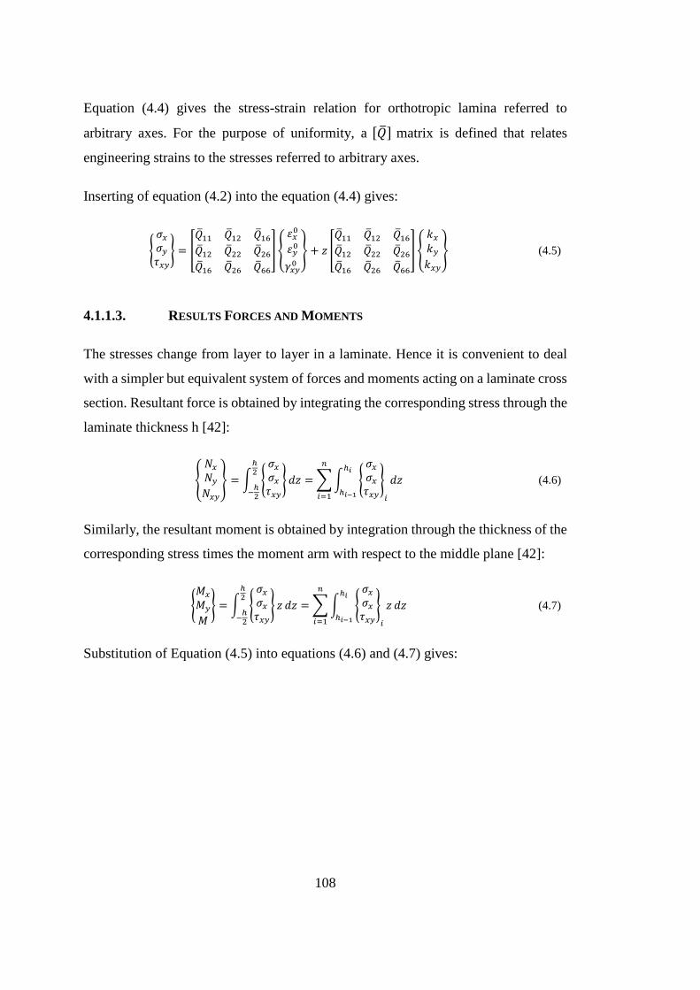
108

Equation (4.4) gives the stress-strain relation for orthotropic lamina referred to

arbitrary axes. For the purpose of uniformity, a [�̅�] matrix is defined that relates

engineering strains to the stresses referred to arbitrary axes.

Inserting of equation (4.2) into the equation (4.4) gives:

{


} = [

�̅�11 �̅�12 �̅�16�̅�12 �̅�22 �̅�26�̅�16 �̅�26 �̅�66

] {

𝜀𝑥0

𝜀𝑦0

𝛾𝑥𝑦0

} + 𝑧 [

�̅�11 �̅�12 �̅�16�̅�12 �̅�22 �̅�26�̅�16 �̅�26 �̅�66

] {


} (4.5)

4.1.1.3. RESULTS FORCES AND MOMENTS

The stresses change from layer to layer in a laminate. Hence it is convenient to deal

with a simpler but equivalent system of forces and moments acting on a laminate cross

section. Resultant force is obtained by integrating the corresponding stress through the

laminate thickness h [42]:

{

𝑁𝑥𝑁𝑦𝑁𝑥𝑦

} = ∫ {

𝜎𝑥𝜎𝑥𝜏𝑥𝑦

} 𝑑𝑧

ℎ2

−ℎ2

=∑∫ {


}

𝑖

𝑑𝑧ℎ𝑖

ℎ𝑖−1

𝑛

𝑖=1

(4.6)

Similarly, the resultant moment is obtained by integration through the thickness of the

corresponding stress times the moment arm with respect to the middle plane [42]:

{𝑀𝑥

𝑀𝑦

𝑀

} = ∫ {


} 𝑧 𝑑𝑧

ℎ2

−ℎ2

=∑∫ {


}

𝑖

𝑧 𝑑𝑧ℎ𝑖

ℎ𝑖−1

𝑛

𝑖=1

(4.7)

Substitution of Equation (4.5) into equations (4.6) and (4.7) gives:

109

{


} =∑∫ [

�̅�11 �̅�12 �̅�16�̅�12 �̅�22 �̅�26�̅�16 �̅�26 �̅�66

]

𝑖

𝑑𝑧ℎ𝑖

ℎ𝑖−1

𝑛

𝑖=1

{

𝜀𝑥0

𝜀𝑦0

𝛾𝑥𝑦0

}

+∑∫ 𝑧 [

�̅�11 �̅�12 �̅�16�̅�12 �̅�22 �̅�26�̅�16 �̅�26 �̅�66

]

𝑖

𝑑𝑧ℎ𝑖

ℎ𝑖−1

𝑛

𝑖=1

{


}

= [

𝐴11 𝐴12 𝐴16𝐴12 𝐴22 𝐴26𝐴16 𝐴26 𝐴66

]

{


𝜕𝑢0𝜕𝑦

+𝜕𝑣0𝜕𝑥 }

+ [

𝐵11 𝐵12 𝐵16𝐵12 𝐵22 𝐵26𝐵16 𝐵26 𝐵66

]

{

−

𝜕2𝑤0𝜕𝑥2

−𝜕2𝑤0𝜕𝑦2

−2𝜕2𝑤0𝜕𝑥𝜕𝑦}

(4.8)

{𝑀𝑥

𝑀𝑦

𝑀

} =∑∫ 𝑧 [

�̅�11 �̅�12 �̅�16�̅�12 �̅�22 �̅�26�̅�16 �̅�26 �̅�66

]

𝑖

𝑑𝑧ℎ𝑖

ℎ𝑖−1

𝑛

𝑖=1

{

𝜀𝑥0

𝜀𝑦0

𝛾𝑥𝑦0

}

+∑∫ 𝑧2 [

�̅�11 �̅�12 �̅�16�̅�12 �̅�22 �̅�26�̅�16 �̅�26 �̅�66

]

𝑖

𝑑𝑧ℎ𝑖

ℎ𝑖−1

𝑛

𝑖=1

{


}

= [

𝐵11 𝐵12 𝐵16𝐵12 𝐵22 𝐵26𝐵16 𝐵26 𝐵66

]

{


𝜕𝑢0𝜕𝑦

+𝜕𝑣0𝜕𝑥 }

+ [

𝐷11 𝐷12 𝐷16𝐷12 𝐷22 𝐷26𝐷16 𝐷26 𝐷66

]

{

−

𝜕2𝑤0𝜕𝑥2

−𝜕2𝑤0𝜕𝑦2

−2𝜕2𝑤0𝜕𝑥𝜕𝑦}

(4.9)

4.1.1.4. EQUILIBRIUM EQUATIONS IN TERMS OF DISPLACEMENT

Equilibrium of forces in x, y direction for laminated thin plates are given in Equations

(4.10) and (4.11), respectively. In addition, governing equation for buckling analysis

for laminated thin plates is given in Equation (4.12) . In the Appendix D.2, calculations

of these equations are given in Equations (D.12), (D.13) and (D.25).

𝜕𝑁𝑥𝜕𝑥

+𝜕𝑁𝑥𝑦

𝜕𝑦= 0

(4.10)

𝜕𝑁𝑦

𝜕𝑦+𝜕𝑁𝑥𝑦

𝜕𝑥= 0

(4.11)

𝜕2𝑀𝑥

𝜕𝑥2+𝜕2𝑀𝑥𝑦

𝜕𝑥𝜕𝑦+𝜕2𝑀𝑦

𝜕𝑦2+ 𝑝∗ = 0 (4.12)

110

Where: 𝑝∗ = 𝑝 + 𝑁𝑥𝜕2𝑤

𝜕𝑥2+ 𝑁𝑦

𝜕2𝑤

𝜕𝑦2+ 2𝑁𝑥𝑦

𝜕2𝑤

𝜕𝑥𝜕𝑦− 𝜌∗

𝜕2𝑤

𝜕𝑡2

Equation (4.12) is used for the solution of the buckling load. Inserting Equation (4.9)

into the Equation (4.12), we obtain:

−𝐷11𝜕4𝑤

𝜕𝑥4− 4𝐷16

𝜕4𝑤

𝜕𝑥3𝜕𝑦− (2𝐷12 + 4𝐷66)

𝜕4𝑤

𝜕𝑥2𝜕𝑦2− 4𝐷26

𝜕4𝑤

𝜕𝑦3𝜕𝑥− 𝐷22

𝜕4𝑤

𝜕𝑦4+

𝐵11𝜕3𝑢0𝜕𝑥3

+ 3𝐵16𝜕3𝑢0𝜕𝑥2𝜕𝑦

+ (𝐵12 + 2𝐵66)𝜕3𝑢0𝜕𝑦2𝜕𝑥

+ 𝐵26𝜕3𝑢0𝜕𝑦3

+

𝐵16𝜕3𝑣0𝜕𝑥3

+ (𝐵12 + 2𝐵66)𝜕3𝑣0𝜕𝑥2𝜕𝑦

+ 3𝐵26𝜕3𝑣0𝜕𝑦2𝜕𝑥

+ 𝐵22𝜕3𝑣0𝜕𝑦3

+𝑝∗ = 0

(4.13)

For specially orthotropic laminates, their constitutive equations satisfy the following

conditions [42]:

𝐴16 = 𝐴26 = 0

𝐵𝑖𝑗 = 0

𝐷16 = 𝐷26 = 0

(4.14)

Incorporation of conditions above into Equation (4.13) simplifies the equilibrium

equation for specially orthotropic laminates as given by Equation (4.15).

𝐷11𝜕4𝑤

𝜕𝑥4+ (2𝐷12 + 4𝐷66)

𝜕4𝑤

𝜕𝑥2𝜕𝑦2+ 𝐷22

𝜕4𝑤

𝜕𝑦4= 𝑝∗ (4.15)

4.1.2. First Order Shear Deformation Theory (FSDT)

First order shear deformation theory is a bit more complicated compared to CPTL and

it based on the Reissner-Mindlin hypothesis. In this theory, plane cross sections remain

plane after deformation, however it does not have to remain normal to the reference

plane. In this method, out-of-plane shear deformation is also included.

111

4.1.2.1. KINEMATICS

The displacement field for the FSDT based on the assumption is given in Equation

(4.16) [43]. As well, undeformed and deformed geometric descriptions of plate edge

according to first-order plate theory assumptions are seen in the Figure 4.2.

𝑢(𝑥, 𝑦, 𝑧) = 𝑢0 + 𝑧𝜙𝑥, 𝑣(𝑥, 𝑦, 𝑧) = 𝑣0 + 𝑧𝜙𝑦, 𝑤(𝑥, 𝑦, 𝑧) = 𝑤0(𝑥, 𝑦) (4.16)

Where: 𝜙𝑥 =𝜕𝑢

𝜕𝑧, 𝜙𝑦 =

𝜕𝑣

𝜕𝑧

which indicate that 𝜙𝑥 and 𝜙𝑦 are the rotations of the transverse normal about the y

and the x axes, respectively.

Figure 4.2: Undeformed and deformed geometries of an edge of a plate under the assumptions of the

first-order plate theory [43].

It is convenient to split the strain vector into two parts, where 𝜀𝑏 is the axial-bending

part and 𝜀𝑠 is the transverse shear part [44]. Axial and bending strain part of plate is

given in the Equation (4.17), and equation for transverse shear strain of plate is given

in Equation (4.18).

112

𝜀𝑏 = {

𝜀𝑥𝜀𝑦𝛾𝑥𝑦} =

{


𝜕𝑢0𝜕𝑦

+𝜕𝑣0𝜕𝑥 }

+ 𝑧

{

𝜕𝜙𝑥𝜕𝑥𝜕𝜙𝑦

𝜕𝑦

𝜕𝜙𝑥𝜕𝑦

+𝜕𝜙𝑦

𝜕𝑥 }

(4.17)

𝜀𝑠 = {𝛾𝑦𝑧𝛾𝑥𝑧} =

{

𝜕𝑣

𝜕𝑧+𝜕𝑤0𝜕𝑦

𝜕𝑢

𝜕𝑧+𝜕𝑤0𝜕𝑥 }

=

{

𝜙𝑦 +𝜕𝑤0𝜕𝑦

𝜙𝑥 +𝜕𝑤0𝜕𝑥 }

(4.18)

4.1.2.2. MATERIAL LAW

Definition of tensor strains is given by Equation (4.19) [42]:

{

𝜀𝐿𝜀𝑇1

2𝛾𝐿𝑇

} = [𝑇] {

𝜀𝑥𝜀𝑦1

2𝛾𝑥𝑦

} (4.19)

The relations between stresses and strains are obtained utilizing linear elasticity. For

the FSDT, it is useful to split stress-strain relation into two parts, involving axial-

bending and transverse shear. Hence, by using the tensor strains, the axial and bending

part can be expressed as:

{


} = [

�̅�11 �̅�12 �̅�16�̅�12 �̅�22 �̅�26�̅�16 �̅�26 �̅�66

]

{


𝜕𝑢0𝜕𝑦

+𝜕𝑣0𝜕𝑥 }

+ 𝑧 [

�̅�11 �̅�12 �̅�16�̅�12 �̅�22 �̅�26�̅�16 �̅�26 �̅�66

]

{


𝜕𝑦


+𝜕𝜙𝑦

𝜕𝑥 }

(4.20)

Then the transverse-shear part is given as [42]:

{𝜏𝑦𝑧𝜏𝑥𝑧} = 𝑘𝑠𝑐 [

�̅�44 �̅�45�̅�45 �̅�55

] {𝛾𝑦𝑧𝛾𝑥𝑧} = 𝑘 [

�̅�44 �̅�45�̅�45 �̅�55

]

{


𝜙𝑥 +𝜕𝑤0𝜕𝑥 }

(4.21)

where 𝑘𝑠𝑐 is the shear correction coefficient.

113

4.1.2.3. RESULTS FORCES AND MOMENTS

The resultant force and resultant moment are obtained in the same way as the CLPT:

{


} = [

𝐴11 𝐴12 𝐴16𝐴12 𝐴22 𝐴26𝐴16 𝐴26 𝐴66

]

{


𝜕𝑢0𝜕𝑦

+𝜕𝑣0𝜕𝑥 }

+ [

𝐵11 𝐵12 𝐵16𝐵12 𝐵22 𝐵26𝐵16 𝐵26 𝐵66

]

{


𝜕𝑦


+𝜕𝜙𝑦

𝜕𝑥 }

(4.22)

{𝑀𝑥

𝑀𝑦

𝑀

} = [

𝐵11 𝐵12 𝐵16𝐵12 𝐵22 𝐵26𝐵16 𝐵26 𝐵66

]

{


𝜕𝑢0𝜕𝑦

+𝜕𝑣0𝜕𝑥 }

+ [

𝐷11 𝐷12 𝐷16𝐷12 𝐷22 𝐷26𝐷16 𝐷26 𝐷66

]

{


𝜕𝑦


+𝜕𝜙𝑦

𝜕𝑥 }

(4.23)

Equations relating the shear-force resultants 𝑅𝑦𝑧 and 𝑅𝑥𝑧 to the shear strains 𝛾𝑦𝑧 and

𝛾𝑥𝑧 can be written as [42]:

{𝑅𝑦𝑧𝑅𝑥𝑧

} = 𝑘∑∫ [�̅�44 �̅�45�̅�45 �̅�55

] 𝑑𝑧ℎ𝑖

ℎ𝑖−1

𝑛

𝑖=1

{𝛾𝑦𝑧0

𝛾𝑥𝑧0} = 𝑘 [

𝐴44 𝐴45𝐴45 𝐴55

]

{


𝜙𝑥 +𝜕𝑤0𝜕𝑥 }

(4.24)

4.1.2.4. EQUILIBRIUM EQUATIONS IN TERMS OF DISPLACEMENT

Equilibrium of moments in x, y direction for laminated thin plates are given in

Equations (4.25) and (4.26), respectively. In addition, Equilibrium of forces in z

direction for laminated thin plates is given in Equation (4.27). In the Appendix D.2,

calculations of these equations are given in Equations (D.20), (D.22) and (D.24).

𝜕𝑀𝑥

𝜕𝑥+𝜕𝑀𝑥𝑦

𝜕𝑦− 𝑅𝑥𝑧 = 0

(4.25)

𝜕𝑀𝑦

𝜕𝑦+𝜕𝑀𝑥𝑦

𝜕𝑥− 𝑅𝑦𝑧 = 0

(4.26)

𝜕𝑅𝑥𝑧𝜕𝑥

+𝜕𝑅𝑦𝑧

𝜕𝑦+ 𝑝∗ = 0 (4.27)

114

Where: 𝑝∗ = 𝑝 + 𝑁𝑥𝜕2𝑤

𝜕𝑥2+ 𝑁𝑦

𝜕2𝑤

𝜕𝑦2+ 2𝑁𝑥𝑦

𝜕2𝑤

𝜕𝑥𝜕𝑦− 𝜌∗

𝜕2𝑤

𝜕𝑡2

Constitutive equations for a specially orthotropic plate with the new displacement field

still satisfy the conditions stated earlier:

𝐴16 = 𝐴26 = 0

𝐵𝑖𝑗 = 0

𝐷16 = 𝐷26 = 0

𝐴45 = 𝐴54 = 0

(4.28)

In view of these conditions, equilibrium equations above can be written in terms of the

displacement field as follows:

𝐷11𝜕2𝜙𝑥𝜕𝑥2

+ (𝐷12 + 𝐷66)𝜕2𝜙𝑦

𝜕𝑥𝜕𝑦+ 𝐷66

𝜕2𝜙𝑥𝜕𝑦2

− 𝐴55𝑘 (𝜙𝑥 +𝜕𝑤

𝜕𝑥) = 0 (4.29)

𝐷22𝜕2𝜙𝑦

𝜕𝑥2+ (𝐷12 + 𝐷66)

𝜕2𝜙𝑥𝜕𝑥𝜕𝑦

+ 𝐷66𝜕2𝜙𝑦

𝜕𝑦2− 𝐴44𝑘 (𝜙𝑦 +

𝜕𝑤

𝜕𝑦) = 0 (4.30)

𝐴55𝑘 (𝜕𝜙𝑥𝜕𝑥

+𝜕2𝑤

𝜕𝑥2) + 𝐴44𝑘 (

𝜕𝜙𝑦

𝜕𝑦+𝜕2𝑤

𝜕𝑦2) + 𝑝∗ = 0 (4.31)

Equations (4.29)-(4.31) are three coupled second-order differential equations with 𝑤,

𝜙𝑥 and 𝜙𝑦 as the three unknows.

4.2. Analysis of Specially Orthotropic Plates under Uniaxial Compressive Load

using CLPT and FSDT

Calculation methods for critical buckling load of specially orthotropic composite

plates under uniaxial compressive load is studied in this chapter. These calculations

are done using CLPT and FSDT as described early. In addition, boundary condition of

plates are chosen as classical boundary conditions, simply supported and clamped edge

conditions. Composite plate geometric descriptions are given in the Figure 4.3.

115

Figure 4.3: Plate with uniaxial compression load [41].

4.2.1. CLPT

4.2.1.1. BUCKLING OF PLATES WITH SIMPLY SUPPORTED BOUNDARY

CONDITION UNDER UNIAXIAL COMPRESSIVE LOAD

For the buckling analysis, we assume that the only applied load is the in-plane

compressive force in the x direction and all other loads are zero. From equation (4.15)

we put 𝑝∗ = 𝑁𝑥𝜕2𝑤

𝜕𝑥2= −𝑁

𝜕2𝑤

𝜕𝑥2. In this case, the equation governing the buckling

problem is given by:

𝐷11𝜕4𝑤

𝜕𝑥4+ (2𝐷12 + 4𝐷66)

𝜕4𝑤

𝜕𝑥2𝜕𝑦2+ 𝐷22

𝜕4𝑤

𝜕𝑦4+𝑁

𝜕2𝑤

𝜕𝑥2= 0 (4.32)

The plate edges are simply supported so that the transverse displacements at the edges

and resultant moments about each edge are zero. These edge conditions are the

boundary conditions, and mathematically expressed as follows [42]:

𝑥 = 0: 𝑤(0, 𝑦) = 0 𝑀𝑥(0, 𝑦) = 0

𝑥 = 𝑎: 𝑤(𝑎, 𝑦) = 0 𝑀𝑥(𝑎, 𝑦) = 0

𝑦 = 0: 𝑤(𝑥, 0) = 0 𝑀𝑦(𝑥, 0) = 0

𝑦 = 𝑏: 𝑤(𝑥, 𝑏) = 0 𝑀𝑦(𝑥, 𝑏) = 0

(4.33)

116

A Navier solution of equation (4.32) that also satisfies the preceding boundary

conditions is given by [42]:

𝑤(𝑥, 𝑦) = ∑∑ 𝑤𝑚𝑛 sin (𝑚𝜋𝑥

𝑎) sin (

𝑛𝜋𝑦

𝑏)

∞

𝑚=1

∞

𝑛=1

(4.34)

where 𝑤𝑚𝑛 are the displacement coefficients, 𝑚 and 𝑛 are positive integers.

Substituting Equation (4.34) into the Equation (4.32) gives the buckling load as seen

in Equation (4.35).

𝑁 = 𝐷11 (𝑚𝜋

𝑎)2

+ (2𝐷12 + 4𝐷66) (𝑛𝜋

𝑏)2

+ 𝐷22 (𝑎𝜋

𝑚)2

(𝑛

𝑏)4

(4.35)

Thus, for each choice of 𝑚 and 𝑛, there corresponds a unique value of the axial load

N. The critical buckling load is the smallest of N, which can be obtained for n = 1

but m can be any integer number depending on the plate’s geometric configuration.

4.2.1.2. BUCKLING OF PLATES WITH CLAMPED SUPPORTED BOUNDARY


Again, we assume that the only applied load is the in-plane compressive force in the x

direction. For plates with all edges clamped, Rayleigh-Ritz method is used to solve the

buckling problem. The method is based on the plate’s potential energy. We now split

the total potential energy in two parts, bending strain energy and the strain energy due

to external forces [45]:

Π = 𝑈𝑏 + 𝑈𝑝 (4.36)

117

where:

𝑈𝑏 =1

2∫𝜀𝑇𝜎 𝑑𝑉𝑉

=1

2∫ ∫ 𝜀𝑇�̅�𝜀 𝑑𝑧 𝑑𝐴

ℎ2⁄

−ℎ 2⁄𝐴

=1

2∫𝜅𝑇𝐷𝜅 𝑑𝐴𝐴

=1

2∫ ∫ 𝐷11 (

𝜕2𝑤

𝜕𝑥2)

2

+ 2𝐷12 (𝜕2𝑤

𝜕𝑥2) (𝜕2𝑤

𝜕𝑦2) + 𝐷22 (

𝜕2𝑤

𝜕𝑦2)

2𝑎

0

𝑏

0

+ 4𝐷66 (𝜕2𝑤

𝜕𝑥𝜕𝑦)

2

𝑑𝑥 𝑑𝑦

and

(4.37)

𝑈𝑝 =1

2∫ ∫ −𝑁 (

𝜕𝑤

𝜕𝑥)2

𝑑𝑥 𝑑𝑦𝑎

0

𝑏

0

(4.38)

The boundary conditions associated with the clamped edges are given by [41]:

𝑥 = 0: 𝑤(0, 𝑦) = 0 𝜕𝑤(0, 𝑦)

𝜕𝑥= 0

𝑥 = 𝑎: 𝑤(𝑎, 𝑦) = 0 𝜕𝑤(𝑎, 𝑦)

𝜕𝑥= 0

𝑦 = 0: 𝑤(𝑥, 0) = 0 𝜕𝑤(𝑥, 0)

𝜕𝑦= 0

𝑦 = 𝑏: 𝑤(𝑥, 𝑏) = 0 𝜕𝑤(𝑥, 𝑏)

𝜕𝑦= 0

(4.39)

A solution that satisfies the preceding boundary conditions is given by [46]:


𝑎) sin (

𝑛𝜋𝑥

𝑎) sin2 (

𝜋𝑦

𝑏)

∞

𝑚=1

∞

𝑛=1

(4.40)

where 𝑤𝑚𝑛 are the displacement coefficients, 𝑚 and 𝑛 are positive integers.

The equation above with only one term is usually enough to solve the buckling

problem. So we assume that:

118

𝑤(𝑥, 𝑦) = 𝑤𝑚𝑛 sin (𝑚𝜋𝑥

𝑎) sin (

𝑛𝜋𝑦

𝑏) sin2 (

𝜋𝑦

𝑏) (4.41)

Substitution of equation (4.41) into the equation (4.36) gives:

Π =

{

1

2𝜋4𝑤𝑚𝑛

2 [𝐷113

4

𝑏

𝑎3𝑚4 + 𝐷22

3

4

𝑎

𝑏3

+(1

2𝐷12 + 𝐷66)

𝑚2

𝑎𝑏] −

3

32

𝑤𝑚𝑛2 𝜋2𝑏𝑚2

𝑎𝑁,

𝑚 = 𝑛

1

4𝜋4𝑤𝑚𝑛

2 [𝐷113

16

𝑏

𝑎3(𝑛4 + 6𝑚2𝑛2 +𝑚4) + 𝐷22

𝑎

𝑏3

+(1

2𝐷12 + 𝐷66)

𝑛2 +𝑚2

𝑎𝑏] −

3

64

𝑤𝑚𝑛2 𝜋2𝑏(𝑛2 +𝑚2)

𝑎𝑁,

𝑚 ≠ 𝑛

(4.42)

Equilibrium requires that δΠ = 0 , thus:

𝜕Π𝜕𝑤𝑚𝑛

δ𝑤𝑚𝑛 = 0 ↔ 𝜕Π𝜕𝑤𝑚𝑛

= 0 (4.43)

𝜕Π𝜕𝑤𝑚𝑛

=

{

𝜋2𝑤𝑚𝑛[𝐷11𝜋

23

4

𝑏

𝑎3𝑚4 + 𝐷22𝜋

23

4

𝑎

𝑏3

+(1

2𝐷12 + 𝐷66) 𝜋

2𝑚2

𝑎𝑏−3

16

𝑏𝑚2

𝑎𝑁] = 0

𝑚 = 𝑛

1

2𝜋2𝑤𝑚𝑛[𝐷11

3

16

𝑏

𝑎3𝜋2(𝑛4 + 6𝑚2𝑛2 +𝑚4) + 𝐷22

𝑎

𝑏3𝜋2

+(1

2𝐷12 + 𝐷66)

𝜋2

𝑎𝑏(𝑛2 +𝑚2) −

3

16

𝑏

𝑎(𝑛2 +𝑚2)𝑁] = 0

𝑚 ≠ 𝑛

(4.44)

Solving equation (4.44) for N, we obtain:

N

=

{

4𝜋2𝐷11𝑚

2

𝑎3+4𝜋2𝐷22𝑎

2

𝑏4𝑚2+16𝜋2

3𝑏2(1

2𝐷12 + 𝐷66) , 𝑚 = 𝑛

𝐷11𝜋2

𝑎2(𝑛4 + 6𝑚2𝑛2 +𝑚4) + 𝐷22𝜋

2 163𝑎2

𝑏4+ (

12𝐷12 + 𝐷66)

163𝜋2

𝑏2(𝑚2 + 𝑛2)

𝑚2 + 𝑛2, 𝑚 ≠ 𝑛

(4.45

)

Thus, combination of m and n that gives the smallest value of N is the critical buckling

load for a clamped plate.

119

4.2.2. FSDT

4.2.2.1. BUCKLING OF PLATES WITH SIMPLY SUPPORTED BOUNDARY


Since the only applied load is the force in x direction, from equation (4.31), 𝑝∗ =

𝑁𝑥𝜕2𝑤

𝜕𝑥2= −𝑁𝑥

𝜕2𝑤

𝜕𝑥2. Based on equations (4.29)-(4.31), the equation set that is needed

for the solution the buckling problem is given by:

𝐷11𝜕2𝜙𝑥𝜕𝑥2

+ (𝐷12 + 𝐷66)𝜕2𝜙𝑦

𝜕𝑥𝜕𝑦+ 𝐷66

𝜕2𝜙𝑥𝜕𝑦2

− 𝐴55𝑘 (𝜙𝑥 +𝜕𝑤

𝜕𝑥) = 0 (4.46)

𝐷22𝜕2𝜙𝑦

𝜕𝑥2+ (𝐷12 + 𝐷66)

𝜕2𝜙𝑥𝜕𝑥𝜕𝑦

+ 𝐷66𝜕2𝜙𝑦

𝜕𝑦2− 𝐴44𝑘 (𝜙𝑦 +

𝜕𝑤

𝜕𝑦) = 0 (4.47)

𝐴55𝑘 (𝜕𝜙𝑥𝜕𝑥

+𝜕2𝑤

𝜕𝑥2) + 𝐴44𝑘 (

𝜕𝜙𝑦

𝜕𝑦+𝜕2𝑤

𝜕𝑦2)−𝑁

𝜕2𝑤

𝜕𝑥2= 0 (4.48)

Boundary conditions for the simply supported plate are the same as those for the CLPT

given by Equation (4.33). The following double Fourier series are assumed to represent

𝑤, 𝜙𝑥 and 𝜙𝑦 [42]:


𝑎) sin (

𝑛𝜋𝑦

𝑏)

∞

𝑚=1

∞

𝑛=1

(4.49)

𝜙𝑥(𝑥, 𝑦) = ∑∑ 𝑥𝑚𝑛 cos (𝑚𝜋𝑥

𝑎) sin (

𝑛𝜋𝑦

𝑏)

∞

𝑚=1

∞

𝑛=1

(4.50)

𝜙𝑦(𝑥, 𝑦) = ∑∑ 𝑦𝑚𝑛 sin (𝑚𝜋𝑥

𝑎) cos (

𝑛𝜋𝑦

𝑏)

∞

𝑚=1

∞

𝑛=1

(4.51)

where 𝑤𝑚𝑛 , 𝑥𝑚𝑛 and 𝑦𝑚𝑛 are the series coefficients, and 𝑚 and 𝑛 are positive

integers.

Using double Fourier series defined in Equations (4.49) to (4.51), simply supported

boundary conditions defined in Equation (4.33) are satisfied. According to simply

120

supported boundary conditions, 𝑀𝑥 equals to zero when the x is equal to zero. To

verify these series written in above, moment x equilibrium equation written in matrix

equation (4.23) is used and following expression is obtained:

𝑀𝑥 = 𝐷11 ∗𝜕𝜙𝑥𝜕𝑥

+ 𝐷12 ∗𝜕𝜙𝑦

𝜕𝑦 (4.52)

𝑀𝑥 = −𝐷11 ∗ 𝑥𝑚𝑛 ∗𝑚𝜋

𝑎sin (

𝑚𝜋𝑥

𝑎) sin (

𝑛𝜋𝑦

𝑏) − 𝐷12 ∗ 𝑦𝑚𝑛 ∗

𝑛𝜋

𝑏sin (

𝑚𝜋𝑥

𝑎) sin (

𝑛𝜋𝑦

𝑏) (4.53)

When the x value is substituted as zero, 𝑀𝑥 equals to zero as seen in Equation (4.54).

𝑀𝑥(0, 𝑦) = −𝐷11 ∗ 𝑥𝑚𝑛 ∗𝑚𝜋

𝑎sin(0) sin (

𝑛𝜋𝑦

𝑏) − 𝐷12 ∗ 𝑦𝑚𝑛 ∗

𝑛𝜋

𝑏sin(0) sin (

𝑛𝜋𝑦

𝑏) = 0 (4.54)

For simply supported plates, it is enough to consider one term with m and n varying

from each equation. Substitution of equations (4.49)-(4.51) into equations (4.46)-

(4.48) gives the following matrix equation:

[

−𝐷11𝛼2 − 𝐷66𝛽

2 − 𝐴55𝑘 −𝐷12𝛼𝛽 − 𝐷66𝛼𝛽 −𝐴55𝑘𝛼

−𝐷12𝛼𝛽 − 𝐷66𝛼𝛽 −𝐷22𝛽2 − 𝐷66𝛼

2 − 𝐴44𝑘 −𝐴44𝑘𝛽

−𝐴55𝑘𝛼 −𝐴44𝑘𝛽 𝑁𝛼2 − 𝐴55𝑘𝛼2 − 𝐴44𝑘𝛽

2

]

∗ {

𝑥𝑚𝑛𝑦𝑚𝑛𝑤𝑚𝑛

} = {000}

(4.55)

where 𝛼 =𝑚𝜋

𝑎, 𝛽 =

𝑛𝜋

𝑏.

By defining:

𝐶1 = −𝐷11𝛼2 − 𝐷66𝛽

2 − 𝐴55𝑘

𝐶2 = −𝐷12𝛼𝛽 − 𝐷66𝛼𝛽

𝐶3 = −𝐴55𝑘𝛼

𝐶4 = −𝐷22𝛽2 − 𝐷66𝛼

2 − 𝐴44𝑘

𝐶5 = −𝐴44𝑘𝛽

(4.56)

121

Equation (4.55) is simplified to:

[

𝐶1 𝐶2 𝐶3𝐶2 𝐶4 𝐶5𝐶3 𝐶5 𝑁𝛼2 + 𝛼𝐶3 + 𝛽𝐶5

] ∗ {

𝑥𝑚𝑛𝑦𝑚𝑛𝑤𝑚𝑛

} = {000} (4.57)

We are seeking non-trivial solutions, thus,

|

𝐶1 𝐶2 𝐶3𝐶2 𝐶4 𝐶5𝐶3 𝐶5 𝑁𝛼2 + 𝛼𝐶3 + 𝛽𝐶5

| = 0 (4.58)

Solving equation (4.58) for 𝑁, we obtain:

𝑁 =𝐶1𝐶5

2 + 𝛼𝐶3𝐶22 + 𝛽𝐶5𝐶2

2 + 𝐶4𝐶32 − 𝛼𝐶1𝐶3𝐶4 − 𝛽𝐶1𝐶4𝐶5 − 2𝐶2𝐶3𝐶5

𝛼2(𝐶1𝐶4 − 𝐶22)

(4.59)

The critical buckling load occurs at 𝑛 = 1, while 𝑚 can vary.

4.2.2.2. BUCKLING OF PLATES WITH CLAMPED SUPPORTED BOUNDARY


As the CLPT, the Rayleigh-Ritz method has been used to solve the buckling problem

for the clamped plate. It is convenient to split the total potential energy in three parts,

bending, transverse shear and external forces:

Π = 𝑈𝑏 + 𝑈𝑠 + 𝑈𝑝 (4.60)

where:

𝑈𝑏 =1

2∫𝜀𝑏

𝑇𝜎𝑏 𝑑𝑉𝑉

=1

2∫ ∫ 𝜀𝑏

𝑇�̅�𝜀𝑏 𝑑𝑧 𝑑𝐴

ℎ2⁄

−ℎ 2⁄𝐴

=1

2∫𝜅𝑇𝐷𝜅 𝑑𝐴𝐴

=1

2∫ ∫ 𝐷11 (

𝜕2𝑤𝑏𝜕𝑥2

)

2

+ 2𝐷12 (𝜕2𝑤𝑏𝜕𝑥2

)(𝜕2𝑤𝑏𝜕𝑦2

) + 𝐷22 (𝜕2𝑤𝑏𝜕𝑦2

)

2𝑎

0

𝑏

0

+ 4𝐷66 (𝜕2𝑤𝑏𝜕𝑥𝜕𝑦

)

2

𝑑𝑥 𝑑𝑦

(4.61)

122

𝑈𝑠 =1

2∫𝜀𝑠

𝑇𝜎𝑠 𝑑𝑉𝑉

=1

2∫ ∫ 𝜀𝑠

𝑇�̅�𝑠𝑘𝑗𝜀𝑠 𝑑𝑧 𝑑𝐴

ℎ2⁄

−ℎ 2⁄𝐴

=1

2∫𝜀𝑠

𝑇𝐴𝑠𝑘𝑗𝜀𝑠 𝑑𝐴𝐴

=1

2𝑘∫ ∫ 𝐴44 (

𝜕𝑤𝑠𝜕𝑦

)2

+ 𝐴55 (𝜕𝑤𝑠𝜕𝑥

)2


0

𝑏

0

(4.62)

𝑈𝑝 =1

2∫ ∫ −𝑁 (

𝜕𝑤

𝜕𝑥)2


0

𝑏

0

(4.63)

The boundary conditions associated with the clamped edges are again given by

Equation (4.39). A solution that satisfies the preceding boundary conditions is given

by [46]:

𝑤(𝑥, 𝑦) = 𝑤𝑏 + 𝑤𝑠

=∑∑ (w̅b sin (𝑚𝜋𝑥

𝑎) sin (

𝑛𝜋𝑥

𝑎) sin2 (

𝜋𝑦

𝑏)

∞

𝑚=1

∞

𝑛=1

+ w̅s sin (𝑛𝜋𝑥

𝑎) sin (

𝜋𝑦

𝑏))

(4.64)

where w̅band w̅s are the displacement coefficients for bending and transverse shear,

and m and n are positive integers.

For a single term series,

𝑤(𝑥, 𝑦) = w̅b sin (𝑚𝜋𝑥

𝑎) sin (

𝑛𝜋𝑥

𝑎) sin2 (

𝜋𝑦

𝑏) + w̅s sin (

𝑛𝜋𝑥

𝑎) sin (

𝜋𝑦

𝑏) (4.65)

Equilibrium requires that δΠ = 0, thus:

𝜕Π𝜕w̅b

δw̅b +𝜕Π𝜕w̅s

δw̅s = 0 (4.66)

This implies,

{

𝜕Π𝜕w̅b𝜕Π𝜕w̅s}

= {00} (4.67)

123

Firstly, Equation (4.65) is substituted into the Equation (4.60). After that, derivation

of Equations (4.60) gives two solutions as Equation (4.67). Finally, this expression is

divided into two conditions, one for m ≠ 1 and another m = 1.

For m ≠ 1, Equation (4.67) gives following matrix equation:

[𝐻1 + 𝑁𝐻2 𝑁𝐻3𝑁𝐻3 𝐻4 +𝑁𝐻5

] {w̅bw̅s

} = {00} (4.68)

where,

𝐻1 =𝜋4

32𝑎3𝑏3(𝐷11𝑏

4(18𝑚2 + 3 + 3𝑚4) + 𝐷12𝑎2𝑏2(8 + 8𝑚2) + 16𝐷22𝑎

4

+ 𝐷66𝑎2𝑏2(16 + 16𝑚2))

𝐻2 = −𝜋2𝑏(3𝑚6 + 3 + 3𝑛4 − 3𝑚4 − 3𝑚2 + 3𝑚2𝑛4 − 12𝑚2𝑛2 − 6𝑛2 − 6𝑚4𝑛2)

32𝑎(1 − 2𝑛2 +𝑚4 − 2𝑚2𝑛2 − 2𝑚2 + 𝑛4)

𝐻3 = −8𝑏(−𝑚𝑛3 + (−1)𝑚+𝑛+1𝑚𝑛3)

3𝑎(1 − 2𝑛2 +𝑚4 − 2𝑚2𝑛2 − 2𝑚2 + 𝑛4)

𝐻4 =𝑘𝜋2

4𝑎𝑏(𝐴44𝑎

2 + 𝐴55𝑛2𝑏2)

𝐻5 = −𝜋2𝑏(𝑛2 + 𝜋6 − 2𝑚2𝑛4 +𝑚4𝑛2 − 2𝑛4 − 2𝑚2𝑛2)

4𝑎(1 − 2𝑛2 +𝑚4 − 2𝑚2𝑛2 − 2𝑚2 + 𝑛4)

(4.69)

Matrix equation (4.68) gives non-trivial solutions when the determinant of this matrix

expressed is zero. This leads us to a second-order equation:

(𝐻2𝐻5 − 𝐻32)𝑁2 + (𝐻1𝐻5 + 𝐻2𝐻4)𝑁 + 𝐻1𝐻4 = 0 (4.70)

The smallest value of N is given by:

𝑁 =−(𝐻1𝐻5 + 𝐻2𝐻4) − √(𝐻1𝐻5 + 𝐻2𝐻4)

2 − 4(𝐻2𝐻5 − 𝐻32)𝐻1𝐻4

2(𝐻2𝐻5 −𝐻32)

(4.71)

Combination of positive integers m and n gives the critical buckling load.

124

For m = 1, Equation (4.67) gives following matrix equation:

[𝐺1 +𝑁𝐺2 𝑁𝐺3𝑁𝐺3 𝐺4 + 𝑁𝐺5

] {w̅bw̅s

} = {00} (4.72)

where,

𝐺1 =𝜋4

4𝑎3𝑏3(3𝐷11𝑏

4 + 2𝐷12𝑎2𝑏2 + 3𝐷22𝑎

4 + 4𝐷66𝑎2𝑏2)

𝐺2 = −3𝜋2𝑏

16𝑎

𝐺3 = −8𝑏(−𝑛3 + (−1)𝑛+2𝑛3)

3𝑎(𝑛4 − 4𝑛2)

𝐺4 =𝑘𝜋2

4𝑎𝑏(𝐴44𝑎

2 + 𝐴55𝑛2𝑏2)

𝐺5 = −𝜋2𝑏𝑛2

4𝑎

(4.73)

Matrix equation (4.72) gives non-trivial solutions when the determinant of this matrix

expressed is zero. A result of this, a second-order equation is obtained as:

(𝐺2𝐺5 − 𝐺32)𝑁2 + (𝐺1𝐺5 + 𝐺2𝐺4)𝑁 + 𝐺1𝐺4 = 0 (4.74)

Solving this, we obtain the smallest value of N:

𝑁 =−(𝐺1𝐺5 + 𝐺2𝐺4) − √(𝐺1𝐺5 + 𝐺2𝐺4)

2 − 4(𝐺2𝐺5 − 𝐺32)𝐺1𝐺4

2(𝐺2𝐺5 − 𝐺32)

(4.75)

The critical buckling load depends on the positive integer 𝑛.

125

4.3. Finite Element Model of Composite Plates

In this sub-chapter, finite element model description of the composite plate is

explained. Most of the parts of modelling the composite plate are same as the metal

model.

In the finite element model, boundary conditions of the plate are assumed as classical

boundary conditions of the single panel which is defined in Chapter 2.1.

The geometry and the coordinate system of the composite plate are presented in Figure

4.4. Ply orientation angles are given with respect to x axis according to Figure 4.4.

Figure 4.4: Definition of different geometrical parameters of the composite panels and the coordinate

system

In the finite element model of composite plate, plate is modelled as 2D shell elements.

Element type is chosen as quadrilateral element S4R. Element size is decided as 5 mm

based on the mesh size study performed in Chapter 2.1. Moreover, the plate material

is chosen as HexPly 8552 AS4 and at dry and room temperature condition properties

of the composite material are given in Table 4.1. Detailed material properties can be

seen in Appendix E, Figure E.1.

126

Table 4.1: Material properties of HexPly 8552 AS4 composite plate

𝑬𝟏(𝑮𝑷𝒂) 128 ∗ 103 𝑮𝟏𝟐(𝑴𝑷𝒂) 114

𝑬𝟐(𝑮𝑷𝒂) 1 ∗ 103 𝑮𝟏𝟑(𝑴𝑷𝒂) 114

𝒗𝟏𝟐 0.355 𝑮𝟐𝟑(𝑴𝑷𝒂) 114

Load is applied on the DC edge along the y-axis of the single panel as 1 N/mm shell

edge load in the “-x” direction (compression) and the reaction edge of the panel is

chosen as AB edge. In addition, the unloaded edges of the panel are AD and BC.

Finite element model is solved by using the “Buckle” step of ABAQUS [35] in linear

buckling analysis for the lowest buckling eigenvalue and corresponding critical

buckling load.

The critical buckling unit length load is obtained by finite element model using the

lowest eigenvalue as shown in Equation (4.76),

𝑁𝑐𝑟 = 𝑁𝑎𝑝𝑝 ∗ 𝜆𝐹𝐸 (4.76)

where 𝑁𝑎𝑝𝑝 is the compressive shell edge load which is given as 1 N/mm in the “-x”

direction. In addition, 𝜆𝐹𝐸 is the first eigenvalue obtained from finite element analysis.

Then, using the critical buckling load, the affine plate buckling coefficient 𝑘0 is

calculated [47]:

𝑘0 =𝑁𝑐𝑟 ∗ 𝑏

2

𝜋2 ∗ √𝐷11𝐷22 (4.77)

The modified buckling coefficient is calculated as [47]:

𝑘𝑐 = 𝑘0 − 2𝐷∗ (4.78)

where the generalized rigidity ratio 𝐷∗ is given by,

127

𝐷∗ =𝐷12 + 2𝐷66

√𝐷11𝐷22

(4.79)

In addition, plate affine ratio is calculated using equation [47]

𝑎𝑜𝑏𝑜=

𝑎

(𝐷11)1/4

(𝐷22)1/4

𝑏 (4.80)

Using the plate affine ratio and the modified buckling coefficient values of plate,

generic buckling curves for balanced orthotropic rectangular plates can be obtained.

To do that, a Python script is written. Same as in the metallic part in the Chapter 2,

various aspect ratio plates are solved using ABAQUS to obtain the buckling coefficient

curves.

According to the model description made, a script is written Python 2.7 in order to

create an ABAQUS finite element model, run the model and collect the lowest

eigenvalue from the analysis results. The scripts are written for each composite plate

and the following parameters are specified by the user;

• Plate length y

• Plate length x

• Plate material

• Ply thickness

• Ply orientation

• Ply repeat number

• Lay-up symmetry

• Boundary conditions

128

To minimize the time and sources, some of parameters of composite plates are fixed

to certain values as,

• Plate length x = 100 mm

• Plate material = HexPly 8552 UD AS4

• Ply thickness = 0.13 mm

• Lay-up symmetry = True

In this study, one material is demonstrated however material number and type can be

changed by modifying the script given in Appendix F.5.

Discrete values of the design parameters of composite plates are specified in a range.

Upper and lower limits of the design parameters are decided based on the common

used values in the aviation industry.

The following design parameters are specified between the upper and lower limits, and

in total 81 finite element analyses are performed to draw curves for the buckling

coefficients for each configuration. Step size of plate length y is chosen as 5 mm.

• Plate length y = [100:5:500] mm

• Plate boundary conditions = [Simply supported, Clamped]

• Ply repeat number = [2,4]

• Ply configuration

Three different ply configurations are considered in this study.

• (0°/0°)𝑆

• (0°/90°)𝑆

• (45°/0°/−45°/90°)𝑆

129

To minimize the number of finite element analysis, for each parameter minimum of

discrete values are selected within the upper-lower limits of each parameter. Panel

length y has a remarkable effect on the buckling phenomena. Therefore, for the plate

length y, more number of discrete analysis points is used in the finite element analyses.

In addition, ply configuration has also significant effect however it is limited to three

configurations due to lack of source and time.

Generic compressive coefficient buckling curves for balanced, orthotropic and

symmetric composite plates are given in Figure 4.5 to Figure 4.7 for simply supported

boundary conditions. In these figures, there are two curves for each plate thickness

which depends on the ply repeat number and the ply orientation. As seen in Figure 4.5

to Figure 4.7, total thickness of plate is increased however modified buckling coeffient

of plate is decreased. In contrast, this does not mean the buckling load of plate is

decreased when the plate thickness is increased. To see that clearly, a comparison

example is done with plate configuration seen in Table 4.2. The first plate total

thickness is 1.04 mm and the second plate total thickness is 2.08 mm. Plates are

assumed as simply supported at 4 edges.

Table 4.2: Input parameters of the example composite plates used in comparison

Plate material HexPly 8552 UD AS4

Ply thickness (mm) 0.13

Ply configuration (0°/90°)𝑆

Plate length x (mm) 100

Plate length y (mm) 200

Plates bending stiffness properties are calculated using Equation (D.7). Results are

given in Table 4.3.

130

Table 4.3: Thin and thick composite plates thickness and stiffness properties

Thin Plate Thick Plate

Total Thickness (mm) 1.04 2.08

𝑫𝟏𝟏 (𝑵 ∗ 𝒎𝒎) 8617.49 60570.67

𝑫𝟐𝟐 (𝑵 ∗ 𝒎𝒎) 4432.87 43832.17

𝑫𝟏𝟐 (𝑵 ∗ 𝒎𝒎) 316.80 2534.42

𝑫𝟔𝟔 (𝑵 ∗ 𝒎𝒎) 10.69 85.49

Firstly, generalized rigidity ratio of plates are calculated using Equation (4.79). Affine

ratio of plates are calculated with Equation (4.80) using stiffness and geometric

properties given in Table 4.2 and Table 4.3, respectively. After the calculation of affine

ratio, modified buckling coeffient of plates are obtained from Figure 4.6. Then, affine

plate buckling coefficients are calculated for both plates using Equation (4.78). Finally,

buckling load of plates are calculated using Equation (4.77). These results are given in

Table 4.4. As seen in Table 4.4, modified buckling coefficient of thicker plate is less

than thin one. However, buckling load of thicker plate is greater than thin one.

Table 4.4: Buckling load parameters of composite plates used in comparison

Thin Plate Thick Plate

𝑫∗ 0.05 0.05

𝒂𝟎/𝒃𝟎 1.69 1.84

𝒌𝟎 − 𝟐𝑫∗ 6.41 5.14

𝒌𝟎 6.52 5.25

𝑵 (𝑵/𝒎𝒎) 12.66 84.97

131

Figure 4.5: Compressive buckling coefficients for composite plates with simply supported loaded and

unloaded edges (Ply orientation: (0°/0°)𝑆)


unloaded edges (Ply orientation: (0°/90°)𝑆)

132


unloaded edges (Ply orientation: (45°/0°/−45°/90°)𝑆)

Generic compressive buckling coefficient curves for balanced, orthotropic and

symmetric composite plate are given in Figure 4.8 to Figure 4.10 for clamped

boundary conditions.

Figure 4.8: Compressive buckling coefficients for composite plates with clamped loaded and unloaded

edges (Ply orientation: (0°/0°)𝑆)

133

Figure 4.9: Compressive buckling coefficients for composite plates with clamped loaded and unloaded

edges (Ply orientation: (0°/90°)𝑆)

Figure 4.10: Compressive buckling coefficients for composite plates with clamped loaded and

unloaded edges (Ply orientation: (45°/0°/−45°/90°)𝑆)

Buckling behaviour is affected by the total thickness of plate. As seen in the Figure

4.7 and Figure 4.10, thick plates’ buckling coefficient is not affected by the plate aspect

ratio. Moreover, as expected, buckling coefficient of plates with clamped edge

condition is greater than one with the simply supported edge condition in the all ply

configurations.

134

4.4. Comparision of Buckling Coefficient Curves obtained by CLPT, FSDT and

FEA

In this section, buckling coefficient results obtained by the CLPT, FSDT and FEA

methods are compared with each other. In Figure 4.11 and Figure 4.12, buckling

coefficient curves obtained by each method are given for the simply supported

boundary condition and (0°/0°)𝑆 ply orientation.

Figure 4.11: Compare of compressive buckling coefficients with all edges simply supported (Ply

orientation: (0°/0°)𝑆, thickness of plate=1.04 mm)

135



In Figure 4.13 and Figure 4.14, buckling coefficient curves obtained by each method

are given for the simply supported boundary condition and (0°/90°)𝑆 ply orientation.



136




are given for the simply supported boundary condition and (45°/0°/−45°/90°)𝑆ply

orientation.


orientation: (45°/0°/−45°/90°)𝑆, thickness of plate=2.08 mm)

137




are given for the clamped boundary condition and (0°/0°)𝑆 ply orientation.

Figure 4.17: Compare of compressive buckling coefficients with all edges clamped (Ply orientation:

(0°/0°)𝑆, thickness of plate=1.04 mm)

0

2

4

6

8

10

12

14

0 1 2 3 4 5

k0-2

D*

a0/b0

FEA

CLPT

FSDT

138




are given for the clamped boundary condition and (0°/90°)𝑆 ply orientation.



139



In Figure 4.21 and Figure 4.22 buckling coefficient curves obtained by each method

are given for the clamped boundary condition and (45°/0°/−45°/90°)𝑆 ply

orientation.


(45°/0°/−45°/90°)𝑆, thickness of plate=2.08 mm)

140


(45°/0°/−45°/90°)𝑆, thickness of plate=4.16 mm)

In the Figure 4.23 and Figure 4.24, buckling coefficient curves obtained by finite

element analysis for each ply orientation are given at the 2.08 mm plate thickness with

all edges simply supported and clamped, respectively. To achieve the same plate

thickness of 2.08 mm, for the (0°/0°)𝑆 and the (0°/90°)𝑆 ply orientations, 4 ply

repeat is used whereas for the (45°/0°/−45°/90°)𝑆 ply orientation, 2 ply repeat is

used.

Figure 4.23: Compare of compressive buckling coefficients with all edges simply supported at the

same plate thickness (2.08 mm)

141

Figure 4.24: Compare of compressive buckling coefficients with all edges clamped at the same plate

thickness (2.08 mm)

From the buckling coefficient curves presented, the following conclusions are inferred:

• Buckling coefficient curves obtained by the FSDT and FEA agree with each

other considerably well for all laminate configurations and boundary

conditions. For the clamped edge condition, results deviate slightly more

compared to the simply supported edge condition. However, maximum

difference between the FSDT and the FEA results is 3%.

• For composite plates with 0o ply angle, buckling coefficients obtained by the

CLPT, FSDT and FEA agree with each other very well, especially for

laminates with small thickness. As the thickness of the laminate increases,

buckling coefficients obtained by the CLPT deviates from the FSDT and FEA

results.

• For quasi-isotropic laminates having 0o, 90o and ±45o plies, the differences

between the buckling coefficients determined by the finite element analysis

and by the CLPT and FSDT increase. This could be due to the fact that the

displacement forms assumed in the solutions performed by the CLPT and the

FSDT may not represent the actual wave forms of the buckled state. Whereas,

in finite element model, the actual buckled wave form can be predicted more

142

accurately since many elements are used in the finite element model as seen in

Figure 4.25-Figure 4.27.

• For composite plates with 0o ply angle, pattern of buckling coefficient curve

obtained by FEA is similar to pattern of metallic buckling curve.

• At the same plate thickness, for composite plates with all edges simply

supported and 0o and 90o ply angles, buckling coefficient curve obtained by

FEA is slightly different than the composite plate with 0o, 90o ±45o ply angles.

However, patterns of these curves are similar to each other. Moreover, at the

2.08 mm plate thickness, for composite plates with all edges clamped and 0o

and 90o plies, buckling coefficient results obtained by FEA is almost same as

the results of composite plate with 0o, 90o ±45o plies.

• For thicker plates affine ratio of the plate is not effective on the buckling

coefficient.

Figure 4.25: Example view of first buckled mode shape of plate with all edges simply supported (Ply


143





144

145

CHAPTER 5

5. CONCLUSION AND FUTURE WORK

In Chapter 2, the effect of the boundary conditions on the buckling coefficients of

stiffened flat panels is investigated by the finite element analysis. It is noted that

depending on the restraint that the stringer along the unloaded edge of a skin-stringer

panel provides, buckling coefficients obtained from finite element analysis may or may

not agree with the buckling coefficients obtained by the analytical approach using the

classical boundary conditions. For the skin-stringer assemblies with J, Z and T type

stringers, buckling coefficients are determined by the finite element analyses for

various combinations of the geometric properties of skin-stringer assemblies. Loaded

edges of these assemblies are considered as clamped edge conditions. Finite element

database for the buckling coefficients of skin-stringer assemblies for each stringer type

is then processed to generate response surface (RS) and artificial neural network

(ANN) approximations. Response surface and neural network approximations allow

very fast determination of the buckling coefficients of skin-stringer assemblies for the

selected stringer types provided that the geometric properties of the skin-stringer

assembly are within the lower and upper limits of the geometric properties of the skin-

stringer assemblies for which finite element analyses are conducted to generate the RS

and train the ANN. To test the performance of the RS and the ANN generated, 10

additional random data sets are tested for each skin-stringer assembly with J, Z and T

type stringer. It is seen that both the RS and the ANN methods give accurate buckling

146

coefficient results compared to the FEA results. For the skin-stringer assemblies with

three stringer types, it is concluded that the ANN gives more accurate results compared

to the RS. However, it is noted that ANN also has accuracy problems if the parameters

of the ANN are not selected appropriately. To select the proper parameter set for the

ANN, trial and error methodology is used. For instance, if the neuron number is lower

than required neuron number, ANN gives inaccurate results. In addition, if the neuron

number is higher than required neuron number, overfitting occurs in the ANN results.

Therefore, required neuron number is decided with trial and error for each problem

separately. Additionally, number of data sets is also very important in obtaining

accurate ANN and RS. For the randomly selected 10 additional design sets, RMS

values of the ANN are obtained as 0.0494, 0.0544, 0.0458 for the skin-stringer

assemblies with J, Z and T type stringers, respectively. It is to be noted that buckling

coefficients are in the range of 6-8 for the skin-stringer assemblies with J, Z and T type

stringers. It is seen that for the 10 additional analyses for each stringer type, root mean

square errors are very small compared to the magnitude of the buckling coefficients.

This shows that ANN approximation produces very accurate buckling coefficients and

it is deemed that such a fast and accurate approximate solver for the buckling

coefficients based on ANN can be effectively used within the framework of

optimization of skin-stringer assemblies.

In chapter 3, a comparative study on the post-buckling load redistribution in stiffened

aircraft panels modeled with and without material nonlinearity is presented. For this

purpose, a baseline stiffened panel is generated for the investigation of the material

nonlinearity on the post-buckling behavior and on the effective width of the stiffened

panel. To make a direct comparison with the classical empirical approach for the

determination of the effective width of the skin panel, a stiffener section which

provides classical clamped edge condition is designed by matching the compression

buckling coefficient determined by the finite element analysis to the buckling

coefficient of the panel with the classical clamped edge boundary condition. Post-

buckling analysis of the skin-stringer assembly is performed utilizing linear and

nonlinear material models in the finite element analysis to study the effect of material

plasticity on the post-buckling behavior of the skin-stringer assembly.

147

Results are presented on the post-buckling behavior of skin-stringer assemblies with

linear and nonlinear material properties in the finite element model for I, J and Z

stringer shapes for the same panel dimensions. Load distributions obtained by the finite

element analysis performed by the linear and nonlinear material models in the post-

buckled stage revealed that for the skin-stringer assembly with the nonlinear material

model, the peak load is significantly lower than the peak load for the linear material

model case. Effective widths calculated by the finite element based analysis by

employing nonlinear material property are higher than the effective widths calculated

by employing linear material property. Since the peak loads drop when nonlinear

material property is used in the finite element analysis, the increase in the effective

width is considered to be reasonable. If the effective widths calculated by the finite

element analysis employing finite element analysis with nonlinear material properties

are taken as reference, for the skin stringer assemblies studied, classical effective width

formula underestimates the effective widths between 20%-30% except assembly with

Z2 stringer section.

Effective widths calculated by the finite element based analysis by employing linear

material property agree better with the effective widths calculated by the classical

empirical approach of Bruhn compared to the effective widths calculated by the finite

element based analysis by employing nonlinear material property. As an alternative

method, effective widths are also calculated utilizing the stringer stresses determined

by the finite element analysis at the point of collapse in the classical effective width

formula. It is concluded that for skin stringer assemblies with double row fasteners,

effective widths calculated by substituting the stringer stresses at the collapse point

calculated by the finite element analysis in the classical empirical effective width

formula match well with the effective widths calculated by the classical empirical

effective width formula alone. Results of the present analysis also showed that the

classical effective width formula gives reasonable results which are comparable with

the finite element based analysis results.

In the chapter 4, generic compressive buckling curves of composite plates with

different ply orientations are obtained using three different methods. These methods

148

are chosen as the CLPT, FSDT and FEM. To use the CLPT and FSDT methods,

mathematical formulations are shown step by step in sections 4.1 and 4.2. Both simply

supported and clamped edge conditions are investigated using the three methods.

CLPT is chosen because it is the simplest method to determine the critical buckling

load. However, the accuracy of the method is not good when the complexity of the ply

orientations is increased. As the second mathematical method, FSDT is decided

because this method gives the more accurate results compared to CLPT. In the FSDT,

out-of-plane shear deformation is also included. Thus, results of FSDT are more

accurate than the CLPT when compared to the finite element method. As the third and

most realistic method, finite element modelling is chosen to calculate buckling load.

In this study, specific parameters are used to obtain the generic buckling coefficient

curves. These parameters are the modified buckling coefficient and the plate’s affine

ratio. Using these parameters, generic buckling curves for balanced orthotropic

rectangular plates are obtained for three different ply orientation configurations. These

orientations are decided according to use in the aviation industry. These three methods

are applied and buckling coefficient results are obtained for various plates thicknesses,

affine ratios and boundary conditions using a Python script.

Generic buckling coefficient curves are obtained for both simply supported and

clamped edge conditions. As expected, clamped edge results are higher than the simply

supported cases. Moreover, for each ply orientation configuration, buckling curves are

obtained. For the quasi-isotropic plates the effect of the skin thickness is higher on the

buckling coefficients compared to the other configurations. In addition, the effect of

the plate’s affine ratio is not significant in thicker plates. Based on the results obtained

for the composite buckling analysis, it is seen that the buckling coefficient curves

obtained by the FSDT and the FEA agree with each other considerably well for all

laminate configurations and boundary conditions. For the clamped edge condition,

results deviate slightly more compared to the simply supported edge condition.

However, maximum difference between the FSDT and the FEA results is 3%.

As for the future work, the experimental investigation of the post-buckling

phenomenon is deemed to be the most important item. Determination of the post-

149

buckling load distribution experimentally is considered to be a worthwhile study to

conduct as the future study.

150

151

REFERENCES

[1] Bruhn, E. F. (1973). Analysis and design of flight vehicle structures. Indianapolis:

Jacobs Pub.

[2] Paul, A., & George, S. P. (2014, October). Buckling analysis of wing upper skin

panels of a transport aircraft. International Journal of Science, Engineering

and Technology Research, 3(10), 2868-2872.

[3] Gerard, G., & Becker, H. (1957). Handbook of structural stability. Pt. 3. Buckling

of curved plates and shells. Washington: NACA.

[4] Timoshenko, S. P., & Gere, J. M. (1961). Theory of elastic stability. New York:

McGraw-Hill Book.

[5] Bulson, P. (1970). The stability of flat plates. London: Chatto & Windus.

[6] Niu, M. C. (2011). Airframe structural design: practical design information and

data on aircraft structures. Hong Kong: Conmilit Press.

[7] Yu, C. (2003). Buckling of rectangular plates under intermediate and end loads.

MS Thesis, National university of singapore, Department of civil engineering,

Singapore.

[8] Muameleci, M. (2014). Linear and nonlinear buckling analyses of plates using

finite element method. MS Thesis, Linköping university, Department of

management and engineering, Linköping,.

152

[9] Riks, E. (2000). Buckling and post-buckling analysis of stiffened panels in wing

box structures. International Journal of Solids and Structures, 37(46-47),

6795-6824. doi:10.1016/s0020-7683(99)00315-7

[10] Tripp, L. L., Tamekuni, M., & Viswanathan, A. V. (1973). A computer program

for stresses and buckling of heated composite stiffened panels and other

structures. Washington: NASA.

[11] Wittrick, W. H., & Williams, F. W. (1974, April). Buckling and vibration of

anisotropic or isotropic plate assemblies under combined loadings.

International Journal of Mechanical Sciences, 16(4), 209-239.

doi:10.1016/0020-7403(74)90069-1

[12] Murphy, A., Price, M., Gibson, A., & Armstrong, C. (2004). Efficient non-linear

idealisations of aircraft fuselage panels in compression. Finite Elements in

Analysis and Design, 40(13-14), 1977-1993. doi:10.1016/j.finel.2003.11.009

[13] Lynch, C. J., & Sterling, S. (1998). A finite element study of the postbuckling

behaviour of a flat stiffened panel. 21st Congress of International Council of

the Aeronautical Sciences, 1-10.

[14] Weimin, S., Mingbo, T., Liang, G., & Dengke, D. (2008). Post-buckling

simulation of an integral aluminum fuselage panel subjected to axial

compression load. 2008 Asia Simulation Conference - 7th International

Conference on System Simulation and Scientific Computing, 893-897.

doi:10.1109/asc-icsc.2008.4675489

[15] Rhodes, J. (2002). Buckling of thin plates and members and early work on

rectangular tubes. Thin-Walled Structures, 40(2), 87-108. doi:10.1016/s0263-

8231(01)00054-4

[16] Byklum, E., Steen, E., & Amdahl, J. (2004). A semi analytical model for global

buckling and postbuckling analysis of stiffened panels. Thin-Walled

Structures, 42(5), 701-171. doi:10.1016/j.tws.2003.12.006

153

[17] Kopecki, T., & Święch, Ł. (2014). Experimental and numerical analysis of post-

buckling deformation states of integrally stiffened thin-walled components of

load-bearing aircraft structures. Journal of Theoretical and Applied

Mechanics, 52(4), 905-915. doi:10.15632/jtam-pl.52.4.905

[18] Graciano, C., Casanova, E., & Martínez, J. (2011). Imperfection sensitivity of

plate girder webs subjected to patch loading. Journal of Constructional Steel

Research, 67(7), 1128-1133. doi:10.1016/j.jcsr.2011.02.006

[19] Mert, M., & Kayran, A. (2016). Post buckling load redistribution of stiffened

panels in aircraft wingbox structures. 57th AIAA/ASCE/AHS/ASC Structures,

Structural Dynamics, and Materials Conference, 1-12. doi:10.2514/6.2016-

1974

[20] Bedair, O. (2009). Analytical effective width equations for limit state design of

thin plates under non-homogeneous in-plane loading. Archive of Applied

Mechanics, 79(12), 1173-1189. doi:10.1007/s00419-009-0296-z

[21] Dannemann, R. W. (1990). Effective width in elastic postbuckling of thin flanges.

International Specialty Conference on Cold-Formed Steel Structures, 281-297.

[22] Winter, G. (1947). Strength of thin steel compression flanges. Ithaca, NY: Cornell

University.

[23] Sheidaii, M. R., & Bahraminejad, R. (2012). Evaluation of compression member

buckling and post-buckling behavior using artificial neural network. Journal

of Constructional Steel Research, 70, 71-77. doi:10.1016/j.jcsr.2011.10.020

[24] Yildirim, A., Akay, A. A., Gulasik, H., Coker, D., Gurses, E., & Kayran, A.

(2015). Development of bolted flange design tool based on finite element

analysis and artificial neural network. Volume 9: Mechanics of Solids,

Structures and Fluids. doi:10.1115/imece2015-51021

[25] Gomes, H. M., Awruch, A. M., & Lopes, P. A. (2011). Reliability based

optimization of laminated composite structures using genetic algorithms and

154

artificial neural networks. Structural Safety, 33(3), 186-195.

doi:10.1016/j.strusafe.2011.03.001

[26] Gajewski, J., Golewski, P., & Sadowski, T. (2017). Geometry optimization of a

thin-walled element for an air structure using hybrid system integrating

artificial neural network and finite element method. Composite Structures, 159,

589-599. doi:10.1016/j.compstruct.2016.10.007

[27] Sadovský, Z., & Soares, C. G. (2011). Artificial neural network model of the

strength of thin rectangular plates with weld induced initial imperfections.

Reliability Engineering & System Safety, 96(3), 713-717.

doi:10.1016/j.ress.2011.02.010

[28] Lanzi, L., & Giavotto, V. (2006). Post-buckling optimization of composite

stiffened panels: Computations and experiments. Composite Structures, 73(2),

208-220. doi:10.1016/j.compstruct.2005.11.047

[29] Mallela, U. K., & Upadhyay, A. (2016). Buckling load prediction of laminated

composite stiffened panels subjected to in-plane shear using artificial neural

networks. Thin-Walled Structures, 102, 158-164.

doi:10.1016/j.tws.2016.01.025

[30] Cankur, A. (2017). Development of an artificial neural network based analysis

method for skin-stringer structures. Aerospace Engineering. Ankara: Middle

East Technical University.

[31] Yang, Q. J. (2009). Simplified approaches to buckling of composite plates.

Faculty of Mathematics and Natural Science. Oslo: University of Oslo.

[32] Masood, S. N., Viswamurthy, S. R., Gaddikeri, K. M., & Singh, A. K. (2014).

Buckling and postbuckling of cocured composite stiffened panel under axial

compression load. Conference: National Seminar on Aerospace Structures

(NASAS-18), 1-8.

155

[33] Abramovich, H., & Weller, T. (2009). Buckling and postbuckling behavior of

laminated composite stringer stiffened curved panels under axial compression:

Experiments and design guidelines. Journal of Mechanics of Materials and

Structures, 4(7-8), 1187-1207. doi:10.2140/jomms.2009.4.1187

[34] Möcker, T., Linde, P., Kraschin, S., Goetz, F., Marsolek, J., & Wohlers, W.

(2009). Abaqus Fem analysis of the postbuckling behaviour of composite shell

structures. Hamburg: Institute of Composite Structures and Adaptive Systems.

[35] Dassault Systèmes. (2014). Abaqus Analysis User’s Manuel. Retrieved from

Dassault Systèmes: Abaqus Version 6.14

[36] Federal Aviation Administration. (2013). MMPDS-08: Metallic Materials

Properties Development and Standardization. Washington, D.C.

[37] MathWorks. (2016). MATLAB 2016 Help. Retrieved from MathWorks:

MATLAB 2016 Help

[38] Beale, M., Hagan, M., & Demuth, H. (1992). Neural Network Toolbox: For Use

with MATLAB;[User’s Guide]. MathWorks.

[39] Rasmussen, K., Tim, B., & Bezkorovainy, P. (2002). Strength Curves for Metal

Plates in Compression, Research Report No R821. The University of Sydney

Department of Civil Engineering.

[40] Spaink, A. (1999). HSB 53211-01 Compressive strength of short metallic

sections(crippling). Hamburg: Industrie Ausschuss Struktur

Berechnungsunterlagen.

[41] Reddy, J. (1997). Mechanics of Laminated Composite Plates - Theory and

Analysis (1 ed.). USA: CRC Press.

[42] Agarwal, B. D., Broutman, L. J., & Chandrashekhara, K. (2006). Analysis and

Performance of Fiber Composites (3 ed.). USA: Wiley.

156

[43] Reddy, J. (2004). Mechanics of Laminated Composite Plates and Shells (2 ed.).

Texas, USA: CRC Press.

[44] Geir, S. (2007). Forelesningsnotat i MEK4560 Elementmetoden i

Faststoffmekanikk. Oslo: UiO.

[45] Hayman, B. (2008). Forelesningsnotat i MEK4540 Komposittmatarialer og -

konstruksjoner. Oslo: UiO.

[46] Zenkert, D. (2005). An Introduction to Sandwich Structures (Student ed.).

Stockholm.

[47] Brunelle, E., & Oyibo, G. (1983). Generic Buckling Curves for Specially

Orthotropic Rectangular Plates The Institute of Aeronautics and Astronautics.

AIAA, 21(8), 1150-1156.

[48] Hayman, B., Berggreen, C., Lundsgaard-Larsen, C., Delarche, A., Toftegaard, H.,

Dow, R., . . . Douka, C. (2009). Studies of The Buckling of Composite Plates

in Compression. Norway-Denmark-UK-Greece: MARSTUCT.

[49] Jensen, C. (2006). Defects in FRP Panels and their Influence on Compressive

Strength. MS Thesis, Denmark.

[50] Zenkert, D., & Battley, M. (2009). Laminate and Sandwich Structures:

Foundations of Fibre Composites (2 ed.). Lyngby, Denmark: Polyteknisk Forlag.

[51] Hexcel. (2016). Resources/Data Sheets/Prepreg/8552/EU Version. Retrieved

from Hexcel Corporation:

http://www.hexcel.com/user_area/content_media/raw/HexPly_8552_eu_Data

Sheet.pdf

157

APPENDICES

APPENDIX A

A. PROCEDURE OF LINEAR BUCKLING ANALYSIS

In ABAQUS, the procedure of linear buckling analysis is explained in this Appendix

[35]. To obtain the critical buckling load in FEA, singular stiffness matrix has to be

solved. In an eigenvalue buckling problem, loads are sought for which the model

stiffness matrix becomes singular, so that the problem has nontrivial solutions, as

shown in Equation (A.1),

𝐾𝑀𝑁 ∗ 𝑣𝑀 = 0 (A.1)

where 𝐾𝑀𝑁 is the tangent stiffness matrix when the loads are applied, and the 𝑣𝑀 is

the nontrivial displacement solution vector. The applied loads can consist of

distributed loads, pressures, concentrated forces, nonzero prescribed displacements.

The buckling loads are calculated relative to the base state of the structure. If the

eigenvalue buckling procedure is the first step in an analysis, the initial conditions

form the base state; otherwise, the base state is the current state of the model at the end

of the last general analysis step. Thus, the base state can include preloads (“dead”

loads), 𝑃𝑁. The preloads are often zero in classical eigenvalue buckling problems. If

geometric nonlinearity is omitted, the base state geometry is the original configuration

of the body. An incremental loading pattern, 𝑄𝑁 is defined in the eigenvalue buckling

158

prediction step. The magnitude of this loading is not important; it will be scaled by the

load multipliers, 𝜆𝑖 found in the eigenvalue problem:

(𝐾0𝑁𝑀 + 𝜆𝑖 ∗ 𝐾∆

𝑁𝑀) ∗ 𝑣𝑖𝑀 = 0 (A.2)

where

𝐾0𝑁𝑀 is the stiffness matrix corresponding to the base state, which includes the effects

of the preloads, 𝑃𝑁 (if any);

𝐾∆𝑁𝑀is the differential initial stress and load stiffness matrix due to the incremental

loading pattern, 𝑄𝑁 ;

𝜆𝑖 are the eigenvalues;

𝑣𝑖𝑀are the buckling mode shapes (eigenvectors);

M and N refer to degrees of freedom M and N of the whole model; and

“i” refers to the i’th buckling mode.

The critical buckling loads are then given by 𝑃𝑁 + 𝜆𝑖𝑄𝑁. Normally, the lowest value

of 𝝀𝒊 is of interest.

The buckling mode shapes, 𝑣𝑖𝑀 , are normalized vectors and do not represent actual

magnitudes of deformation at the critical load. They are normalized so that the

maximum displacement component is 1.0.

ABAQUS can extract eigenvalues and eigenvectors for symmetric matrices only;

therefore, 𝐾0𝑁𝑀 and 𝐾∆

𝑁𝑀 are symmetrized. If the matrices have significant

unsymmetrical parts, the eigenvalue problem may not be exactly what you expected

to solve.

159

APPENDIX B

B. MATERIAL PROPERTIES ALUMINUM 2024 T3 CLAD SHEET

Figure B.1: Material properties of aluminum 2024 T3 clad sheet [36]

160

Figure B.2: True stress-strain graph of Aluminum 2024 T3 clad sheet [36] [39]

Table B.1: True stress-strain data of Aluminum 2024 T3 clad sheet [36] [39]

Stress (MPa) Strain Stress (MPa) Strain Stress (MPa) Strain

250.45 0 300.89 0.017364 384.92 0.121213

251.49 0.000119 302.22 0.018369 387.59 0.125193

252.52 0.000239 303.56 0.019417 390.31 0.129257

253.56 0.000361 304.92 0.020511 393.09 0.133405

254.60 0.000484 306.30 0.021651 395.91 0.137636

255.64 0.000609 307.69 0.022839 398.78 0.141951

256.68 0.000737 309.10 0.024075 401.70 0.146351

257.72 0.000869 310.53 0.025361 404.68 0.150835

258.76 0.001005 311.98 0.026698 407.70 0.155404

259.80 0.001146 313.45 0.028087 410.79 0.160059

260.85 0.001293 314.94 0.029529 413.92 0.164798

261.89 0.001447 316.44 0.031026 417.12 0.169623

262.94 0.001608 317.98 0.032578 420.37 0.174533

264.00 0.001777 319.53 0.034186 423.68 0.179528

265.05 0.001956 321.10 0.035851 427.04 0.184609

266.11 0.002144 322.70 0.037575 430.47 0.189775

161

Table B.2 Continued

Stress (MPa) Strain Stress (MPa) Strain Stress (MPa) Strain

267.17 0.002343 324.32 0.039359 433.96 0.195027

268.23 0.002554 325.97 0.041204 437.51 0.200364

269.30 0.002778 327.64 0.04311 441.13 0.205786

270.38 0.003015 329.34 0.045079 444.81 0.211293

271.45 0.003267 331.07 0.047111 448.55 0.216885

272.54 0.003535 332.82 0.049209 452.36 0.222562

273.62 0.003819 334.60 0.051372 456.24 0.228323

274.71 0.004121 336.40 0.053602 460.18 0.234168

275.81 0.004441 338.24 0.055899 464.20 0.240097

276.92 0.004781 340.11 0.058265 468.28 0.24611

278.03 0.005141 342.01 0.0607 472.44 0.252206

279.15 0.005524 343.94 0.063205 476.67 0.258385

280.27 0.005929 345.90 0.065782 480.98 0.264646

281.40 0.006358 347.89 0.068431 485.36 0.27099

282.54 0.006812 349.92 0.071153 489.81 0.277415

283.69 0.007292 351.98 0.073948 494.35 0.283921

284.85 0.007798 354.08 0.076818 498.96 0.290508

286.02 0.008334 356.21 0.079763 503.65 0.297175

287.19 0.008898 358.39 0.082784 508.42 0.303922

288.38 0.009493 360.59 0.085881 513.28 0.310747

289.58 0.010119 362.84 0.089056 518.21 0.317651

290.78 0.010779 365.12 0.092309 523.24 0.324633

292.00 0.011471 367.45 0.095641 528.34 0.331691

293.23 0.012199 369.82 0.099052 533.54 0.338827

294.48 0.012963 372.22 0.102543 538.82 0.346038

295.73 0.013764 374.67 0.106114 544.19 0.353324

297.00 0.014604 377.17 0.109766 549.66 0.360684

298.28 0.015483 379.70 0.113499 555.21 0.368118

299.58 0.016403 382.29 0.117315 560.86 0.375625

162

163

APPENDIX C

C. LOCAL BUCKLING STRINGERS IN SKIN-STIFFENER ASSEMBLIES

Local buckling of stiffeners is checked according to the method presented in Bruhn

[1]. Cross-section of the stiffener is divided into rectangular elements and critical stress

for each of these elements is calculated as follows:

𝑘𝑐∗ =

𝑘𝑐 ∗ 𝜋2

12 ∗ (1 − 𝑣2) (C.1)

𝐹𝑙𝑏𝑖 = 𝑘𝑐∗ ∗ 𝐸 ∗ (

𝑡𝑖𝑏𝑖)2

(C.2)

where the index 𝑖 represents the section element, and 𝑘𝑐∗ is the modified buckling

coefficient and for elements supported at one side and simply supported loaded edges

𝑘𝑐∗ values are obtained by averaging case 5 (𝑘𝑐 = 0.406, 𝑘𝑐

∗ = 0.367) and case 4

(𝑘𝑐 = 1.25, 𝑘𝑐∗ = 1.12) in Figure C.1. Similarly, for elements supported at both sides,

𝑘𝑐∗ is defined as average 𝑘𝑐

∗ values of case 3 (𝑘𝑐 = 4.0, 𝑘𝑐∗ = 3.61) and case 1 (𝑘𝑐 =

6.97, 𝑘𝑐∗ = 6.3) in Figure C.1.

After calculating the buckling allowable of each section element, the minimum value

is determined as the local buckling allowable of the whole section.

164

𝐹𝑙𝑏 = 𝑚𝑖𝑛(𝐹𝑙𝑏𝑖) (C.3)

Figure C.1: Buckling factors for several edge conditions [1]

165

APPENDIX D

D. ELASTIC COEFFICIENT AND COMPLIANCE MATRICES AND

GOVERNING EQUILIBRIUM EQUATIONS OF COMPOSITE PLATES

D.1 Elastic Coefficient and Compliance Matrices of Composite Plates

For the first method, CLPT, stiffness matrices are obtained as seen in Equations (D.5),

(D.6) and (D.7). To do that, firstly, compliance matrix is obtained as Equation (D.1).

[S] is known as the compliance tensor. It should be evident that the compliance tensor

has the same symmetric properties as the elastic tensor [E] and same type of

transformation law. The number of independent components of compliance tensor can

be reduced in manner similar to elasticity tensor. At the end, compliance matrix for an

orthotropic material for the two dimensional case is obtained as [42]:

[𝑆] =

[ 1

𝐸1−𝑣21𝐸2

0

−𝑣12𝐸1

1

𝐸20

0 01

𝐺12]

(D.1)

Transformation matrix is found following equation [42]:

[𝑇] = [cos2 𝜃 sin2 𝜃 2 sin 𝜃 cos 𝜃sin2 𝜃 cos2 𝜃 −2 sin 𝜃 cos 𝜃

− sin 𝜃 cos 𝜃 sin 𝜃 cos 𝜃 cos2 𝜃 − sin2 𝜃

] (D.2)

166

Where 𝜃 is the fiber orientation angle.

Stiffness matrix of composite plate is calculated as [42]:

[𝑄] = [𝑆]−1 (D.3)

[�̅�] = [𝑇]−1[𝑄][𝑇] (D.4)

Elements of the Extensional stiffness matrix which is defined as “A” is calculated the

following way [42]:

𝐴𝑖𝑗 =∑(�̅�𝑖𝑗)𝑘(ℎ𝑘 − ℎ𝑘−1)

𝑛

𝑘=1

(D.5)

In addition, elements of the coupling stiffness matrix, “B”, is obtained as [42]:

𝐵𝑖𝑗 =1

2∑(�̅�𝑖𝑗)𝑘

(ℎ𝑘2 − ℎ𝑘−1

2 )

𝑛

𝑘=1

(D.6)

Moreover, elements of the bending stiffness matrix, “D”, are given as [42]:

𝐷𝑖𝑗 =1

3∑(�̅�𝑖𝑗)𝑘

(ℎ𝑘3 − ℎ𝑘−1

3 )

𝑛

𝑘=1

(D.7)

Where 𝑖 = 1,2,3 and 𝑗 = 1,2,3. “ℎ𝑘” is the vertical distance from mid-plane of the

plate (z=0) to the upper surface of the kth lamina (layer) as seen in Figure D.1 .

167

Figure D.1: Cross section view of a laminate

For the second method, FSDT, plane shear term has to be added into the formulation.

Shear correction factor is used in the determination of the transverse shear stiffness

matrix. Shear correction factor is obtained from Table D.1.

Table D.1: Typical shear correction coefficient [49]

Material Type Homogeneous Composite Sandwich

Shear Correction Factor 5/6 5/6 1

168

Transverse shear stiffness matrix of a ply is given by [43]:

[𝑄]𝑠ℎ𝑟 = [𝐺23 00 𝐺13

] (D.8)

Transformation matrix for shear part is obtained as [43]:

[𝑇]𝑠ℎ𝑟 = [cos 𝜃 − sin 𝜃sin 𝜃 cos 𝜃

] (D.9)

Transformed transverse shear stiffness matrix for a ply is calculated as [42]:

[�̅�]𝑠ℎ𝑟 = [𝑇]𝑠ℎ𝑟−1 [𝑄]𝑠ℎ𝑟[𝑇]𝑠ℎ𝑟 (D.10)

Finally, transverse shear stiffness matrix for the laminate is obtained as [43]:

(𝐴𝑖𝑗)𝑠ℎ𝑟 = 𝑘𝑠ℎ𝑟∑((�̅�𝑖𝑗)𝑘)𝑠ℎ𝑟(ℎ𝑘 − ℎ𝑘−1)

𝑛

𝑘=1

(D.11)

Where 𝑖 = 4,5 and 𝑗 = 4,5.

D.2 Governing Equations of Composite Plates

Figure D.2 and Figure D.3 show the infinitesimally small elements with the resultant

forces and moments to obtain the force and moment equivalence equations in the

composite plate buckling. For equilibrium, resultant forces and moments are zero.

Figure D.2: A differential element with in-plane force resultants [42]

169

Figure D.3: A differential element with moment resultants, shear force resultants and applied

transverse forces [42]

Equilibrium of forces in the x direction according to Figure D.2 is obtained as:

−𝑁𝑥 𝑑𝑦 + (𝑁𝑥 +𝜕𝑁𝑥𝜕𝑥

𝑑𝑥) 𝑑𝑦 − 𝑁𝑥𝑦 𝑑𝑥 + (𝑁𝑥𝑦 +𝜕𝑁𝑥𝑦

𝜕𝑦𝑑𝑦) 𝑑𝑥 = 0

⟹𝜕𝑁𝑥𝜕𝑥

+𝜕𝑁𝑥𝑦

𝜕𝑦= 0

(D.12)

Equilibrium of forces in the y direction according to Figure D.2 is obtained as:

−𝑁𝑦 𝑑𝑥 + (𝑁𝑦 +𝜕𝑁𝑦

𝜕𝑦𝑑𝑦)𝑑𝑥 − 𝑁𝑥𝑦 𝑑𝑦 + (𝑁𝑥𝑦 +

𝜕𝑁𝑥𝑦

𝜕𝑥𝑑𝑥) 𝑑𝑦 = 0

⟹𝜕𝑁𝑦


𝜕𝑥= 0

(D.13)

Equilibrium of forces in the z direction according to Figure D.2 is obtained with the

projection of transverse normal forces as:

−𝑅𝑥𝑧 𝑑𝑦 + (𝑅𝑥𝑧 +𝜕𝑅𝑥𝑧𝜕𝑥

𝑑𝑥) 𝑑𝑦 − 𝑅𝑦𝑧 𝑑𝑥 + (𝑅𝑦𝑧 +𝜕𝑅𝑦𝑧

𝜕𝑦𝑑𝑦) 𝑑𝑥 + 𝑝 𝑑𝑥 𝑑𝑦 = 0

⟹𝜕𝑅𝑥𝑧𝜕𝑥

+𝜕𝑅𝑦𝑧

𝜕𝑦+ 𝑝 = 0

(D.14)

According to Figure D-3, contributions of the in-plane normal and shear forces in the

z direction are given by:

170

−𝑁𝑥𝜕𝜔

𝜕𝑥𝑑𝑦 + (𝑁𝑥 +


𝑑𝑥) 𝑑𝑦 (𝜕𝜔

𝜕𝑥+𝜕2𝜔

𝜕𝑥2𝑑𝑥) = 𝑁𝑥

𝜕2𝜔

𝜕𝑥2𝑑𝑥𝑑𝑦 +


𝜕𝜔

𝜕𝑥𝑑𝑥𝑑𝑦 (D.15)

−𝑁𝑦𝑥𝜕𝜔

𝜕𝑥𝑑𝑦 + (𝑁𝑥𝑦 +

𝜕𝑁𝑦𝑥

𝜕𝑦𝑑𝑦) 𝑑𝑥 (

𝜕𝜔

𝜕𝑥+𝜕2𝜔

𝜕𝑥𝜕𝑦𝑑𝑦)

= 𝑁𝑦𝑥𝜕2𝜔

𝜕𝑥𝜕𝑦𝑑𝑥𝑑𝑦 +

𝜕𝑁𝑦𝑥

𝜕𝑦

𝜕𝜔

𝜕𝑥𝑑𝑥𝑑𝑦

(D.16)

−𝑁𝑦𝜕𝜔

𝜕𝑦𝑑𝑥 + (𝑁𝑦 +

𝜕𝑁𝑦

𝜕𝑦𝑑𝑦) 𝑑𝑥 (

𝜕𝜔

𝜕𝑦+𝜕2𝜔

𝜕𝑦2𝑑𝑦) = 𝑁𝑦

𝜕2𝜔

𝜕𝑦2𝑑𝑥𝑑𝑦 +

𝜕𝑁𝑦

𝜕𝑦

𝜕𝜔

𝜕𝑦𝑑𝑥𝑑𝑦

(D.17)

−𝑁𝑥𝑦𝜕𝜔

𝜕𝑦𝑑𝑦 + (𝑁𝑥𝑦 +

𝜕𝑁𝑥𝑦

𝜕𝑥𝑑𝑥) 𝑑𝑦 (

𝜕𝜔

𝜕𝑦+𝜕2𝜔

𝜕𝑥𝜕𝑦𝑑𝑥)

= 𝑁𝑥𝑦𝜕2𝜔

𝜕𝑥𝜕𝑦𝑑𝑥𝑑𝑦 +

𝜕𝑁𝑥𝑦

𝜕𝑥

𝜕𝜔

𝜕𝑦𝑑𝑥𝑑𝑦

(D.18)

Figure D.4: Force projection of in-plane normal and shear forces in the z direction [50]

At the end of the equilibrium in the z direction including force projection, Equation

(D.19) is obtained after summing all contributions of the in-plane forces using the

equations (D.15), (D.16), (D.17) and (D.18) and omitting higher order terms in 𝑑𝑥 and

𝑑𝑦.

𝑁𝑥𝜕2𝜔

𝜕𝑥2𝑑𝑥𝑑𝑦 + 𝑁𝑦𝑥

𝜕2𝜔

𝜕𝑥𝜕𝑦𝑑𝑥𝑑𝑦 + 𝑁𝑦

𝜕2𝜔

𝜕𝑦2𝑑𝑥𝑑𝑦 + 𝑁𝑥𝑦

𝜕2𝜔

𝜕𝑥𝜕𝑦𝑑𝑥𝑑𝑦

+𝜕𝜔

𝜕𝑦𝑑𝑥𝑑𝑦 (

𝜕𝑁𝑦


𝜕𝑥) +

𝜕𝜔

𝜕𝑥𝑑𝑥𝑑𝑦 (


+𝜕𝑁𝑥𝑦

𝜕𝑦)

= 𝑁𝑥𝜕2𝜔

𝜕𝑥2+ 𝑁𝑦

𝜕2𝜔

𝜕𝑦2+ 2𝑁𝑦𝑥

𝜕2𝜔

𝜕𝑥𝜕𝑦

(D.19)

171

Then, the final expression for the equilibrium in the z direction is obtained by summing

the transverse forces given in Equation (D.14) and in-plane normal and shear forces

given in Equation (D.19) as:


+𝜕𝑅𝑦𝑧

𝜕𝑦+ 𝑝 + 𝑁𝑥

𝜕2𝜔

𝜕𝑥2+ 𝑁𝑦

𝜕2𝜔


𝜕2𝜔

𝜕𝑥𝜕𝑦− 𝜌∗

𝜕2𝜔

𝜕𝑡2= 0 (D.20)

where 𝜌∗ is the surface weight or mass of the plate.

After obtaining the equations for the force equilibrium, moment equilibrium equations

are obtained in all directions using Figure D.3. In all moment equations, high order

terms are neglected for the simplicity.

Equilibrium of moments in x direction according to Figure D.3 is obtained as:

𝑀𝑦 𝑑𝑥 + (𝑀𝑦 +𝜕𝑀𝑦

𝜕𝑦𝑑𝑦)𝑑𝑥 + 𝑀𝑥𝑦 𝑑𝑦 − (𝑀𝑥𝑦 +

𝜕𝑀𝑥𝑦

𝜕𝑥𝑑𝑥) 𝑑𝑦

+ (𝑅𝑦𝑧 +𝜕𝑅𝑦𝑧

𝜕𝑦𝑑𝑦) 𝑑𝑥 𝑑𝑦 + (𝑅𝑥𝑧 +


𝑑𝑥) 𝑑𝑦𝑑𝑦

2− 𝑅𝑥𝑧 𝑑𝑦

𝑑𝑦

2

+ 𝑝𝑑𝑥 𝑑𝑦𝑑𝑦

2= 0

(D.21)

Equation (D.21) is divided into “𝑑𝑥 𝑑𝑦” terms after that high order derivative terms

are neglected. The moment equation in the x direction simplifies to:

𝜕𝑀𝑦

𝜕𝑦+𝜕𝑀𝑥𝑦

𝜕𝑥− 𝑅𝑦𝑧 = 0 (D.22)

Equilibrium of moments in the y direction according to Figure D.3 is obtained as:

𝑀𝑥 𝑑𝑦 + (𝑀𝑥 +𝜕𝑀𝑥

𝜕𝑥𝑑𝑥) 𝑑𝑦 + 𝑀𝑥𝑦 𝑑𝑥 − (𝑀𝑥𝑦 +

𝜕𝑀𝑥𝑦

𝜕𝑦𝑑𝑦) 𝑑𝑥

+ (𝑅𝑥𝑧 +𝜕𝑅𝑥𝑧𝜕𝑥

𝑑𝑥) 𝑑𝑥 𝑑𝑦 + (𝑅𝑦𝑧 +𝜕𝑅𝑦𝑧

𝜕𝑦𝑑𝑦) 𝑑𝑥

𝑑𝑥

2− 𝑅𝑦𝑧 𝑑𝑥

𝑑𝑥

2

+ 𝑝𝑑𝑥 𝑑𝑦𝑑𝑦

2= 0

(D.23)

Same as the x direction, simple version of moment equation in the y direction is

determined as:

172

𝜕𝑀𝑥

𝜕𝑥+𝜕𝑀𝑥𝑦

𝜕𝑦− 𝑅𝑥𝑧 = 0 (D.24)

Finally, Equation (D.25) is obtained by substituting Equations (D.22) and (D.24) into

the Equation (D.20) as the governing equation for buckling analysis.

𝜕2𝑀𝑥

𝜕𝑥2+ 2

𝜕2𝑀𝑥𝑦

𝜕𝑥𝜕𝑦+𝜕2𝑀𝑦

𝜕𝑦2+ 𝑝 + 𝑁𝑥

𝜕2𝜔

𝜕𝑥2+ 𝑁𝑦

𝜕2𝜔


𝜕2𝜔

𝜕𝑥𝜕𝑦− 𝜌∗

𝜕2𝜔

𝜕𝑡2= 0 (D.25)

173

APPENDIX E

E. MATERIAL PROPERTIES HEXPLY 8552 AS4

Figure E.1: Material properties of HexPly 8552 AS4 at dry and room temperature [51]

174

175

APPENDIX F

F. SCRIPTS

F.1 Linear Metal Single Panel Buckling Python Scripts

# Importing necessary modules from part import * from material import * from section import * from assembly import * from step import * from interaction import * from load import * from mesh import * from optimization import * from job import * from sketch import * from visualization import * from connectorBehavior import * import math # Skin geometric properties sk_x = 100.0 sk_z = 0.0 sk_t = 2.0 # Material properties Ec = 73774.0 E = 72395.0 density = 2768.0 poisson = 0.33 Fcy = 269.0 nc = 15.0 # Applied shell edge load flow = 1.0

176

#Paths save_path = r'C:\Users\…………………….\Single Panel\Model\sp_comp' # Loop for boundary conditions for bc_type in ['ss','cl']: # Loop for applied load type for load_type in ['comp','shear']: #Paths model_path = r'C:\Users\……………………\Single Panel\Model\sp_'+bc_type+'_'+load_type result_path = r'C:\Users\……………………\Single Panel\Result\sp_'+bc_type+'_'+load_type # Initialize output file results = open(result_path+'.csv',"w+") results.write("Ratio FEM Bruhn\n") # Creating panels with different edge length ratio for sk_y in range(100, 505, 5): # Defining model name modelname = 'sp_'+ bc_type +'_'+ load_type +'_'+ str(sk_y) mdb.Model(modelType=STANDARD_EXPLICIT, name=modelname) mn = mdb.models[modelname] # Creating sketch of panel mn.ConstrainedSketch(name='__profile__', sheetSize=200.0) mn.sketches['__profile__'].rectangle(point1=(0.0, 0.0),point2=(sk_x, sk_y)) # Creating part of panel mn.Part(dimensionality=THREE_D, name='panel', type=DEFORMABLE_BODY) mn.parts['panel'].BaseShell(sketch=mn.sketches['__profile__']) del mn.sketches['__profile__'] # Creating material mn.Material(name='AL2024') mn.materials['AL2024'].Elastic(table=((Ec, poisson), )) mn.materials['AL2024'].Density(table=((density, ), )) # Assigning section of panel mn.HomogeneousShellSection(idealization=NO_IDEALIZATION, integrationRule=SIMPSON, material='AL2024', name='Section-1', numIntPts=5, poissonDefinition=DEFAULT, preIntegrate=OFF, temperature=GRADIENT, thickness=sk_t, thicknessField='', thicknessModulus=None, thicknessType= UNIFORM, useDensity=OFF) mn.parts['panel'].Set(faces= mn.parts['panel'].faces.getSequenceFromMask(('[#1 ]', ), ), name='Set-1') mn.parts['panel'].SectionAssignment(offset=0.0, offsetField= '', offsetType=MIDDLE_SURFACE, region= mn.parts['panel'].sets['Set-1'], sectionName='Section-1', thicknessAssignment=FROM_SECTION) # Mesh control mn.parts['panel'].setMeshControls(elemShape=QUAD, regions= mn.parts['panel'].faces.getSequenceFromMask(('[#1 ]', ), ), technique=SWEEP) # Creating mesh seeds of panel mn.parts['panel'].seedPart(deviationFactor=0.1, minSizeFactor=0.1, size=5.0) # Generating mesh

177

mn.parts['panel'].generateMesh() mn.rootAssembly.DatumCsysByDefault(CARTESIAN) mn.rootAssembly.Instance(dependent=ON, name='panel-1', part= mn.parts['panel']) # Creating the set from panel upper edge nodes upedge = mn.parts['panel'].edges.findAt(((sk_x/2.0,sk_y,sk_z),)) upgeoset = mn.parts['panel'].Set(name = 'geoset', edges = upedge) nodenums = [] for node in upgeoset.nodes: nodenums.append(node.label) fnodenum = [nodenums[0]] mn.parts['panel'].SetFromNodeLabels(name = 'up corner', nodeLabels = tuple(fnodenum)) mn.parts['panel'].SetFromNodeLabels(name = 'up nodes', nodeLabels = tuple(nodenums)) # Creating set from panel rigth edge nodes riedge = mn.parts['panel'].edges.findAt(((sk_x,sk_y/2.0,sk_z),)) rigeoset = mn.parts['panel'].Set(name = 'geoset', edges = riedge) nodenums = [] for node in rigeoset.nodes: nodenums.append(node.label) mn.parts['panel'].SetFromNodeLabels(name = 'rigth nodes', nodeLabels = tuple(nodenums)) # Creating set from panel left edge nodes leedge = mn.parts['panel'].edges.findAt(((0.0,sk_y/2.0,sk_z),)) legeoset = mn.parts['panel'].Set(name = 'geoset', edges = leedge) nodenums = [] for node in legeoset.nodes: nodenums.append(node.label) mn.parts['panel'].SetFromNodeLabels(name = 'left nodes', nodeLabels = tuple(nodenums)) # Creating set from panel down edge nodes doedge = mn.parts['panel'].edges.findAt(((sk_x/2.0,0.0,sk_z),)) dogeoset = mn.parts['panel'].Set(name = 'geoset', edges = doedge) nodenums = [] for node in dogeoset.nodes: nodenums.append(node.label) fnodenum = [nodenums[(len(nodenums)-1)]] mn.parts['panel'].SetFromNodeLabels(name = 'down corner', nodeLabels = tuple(fnodenum)) mn.parts['panel'].SetFromNodeLabels(name = 'down nodes', nodeLabels = tuple(nodenums)) # Creating buckling step with subspace solver mn.BuckleStep(description='buckling', maxIterations=3000, vectors=10, name='Step-1', numEigen=3, previous='Initial', eigensolver=SUBSPACE ) # Defining boundary conditions of panel if bc_type=='ss': mn.DisplacementBC(amplitude=UNSET, buckleCase= PERTURBATION_AND_BUCKLING, createStepName='Step-1', distributionType= UNIFORM, fieldName='', fixed=OFF, localCsys=None, name='up_cor', region= mn.rootAssembly.instances['panel-1'].sets['up corner'], u1=0.0, u2=0.0, u3=0.0, ur1=UNSET, ur2=UNSET, ur3=UNSET) mn.DisplacementBC(amplitude=UNSET, buckleCase= PERTURBATION_AND_BUCKLING, createStepName='Step-1', distributionType= UNIFORM, fieldName='', fixed=OFF, localCsys=None, name='down_cor', region= mn.rootAssembly.instances['panel-1'].sets['down corner'], u1=UNSET, u2=0.0, u3=0.0, ur1=UNSET, ur2=UNSET, ur3=UNSET) mn.DisplacementBC(amplitude=UNSET, buckleCase= PERTURBATION_AND_BUCKLING, createStepName='Step-1', distributionType= UNIFORM, fieldName='', fixed=OFF, localCsys=None, name='down', region= mn.rootAssembly.instances['panel-1'].sets['down nodes'], u1=UNSET, u2=UNSET,

178

u3=0.0, ur1=UNSET, ur2=UNSET, ur3=UNSET) mn.DisplacementBC(amplitude=UNSET, buckleCase= PERTURBATION_AND_BUCKLING, createStepName='Step-1', distributionType= UNIFORM, fieldName='', fixed=OFF, localCsys=None, name='up', region= mn.rootAssembly.instances['panel-1'].sets['up nodes'], u1=UNSET, u2=UNSET, u3=0.0, ur1=UNSET, ur2=UNSET, ur3=UNSET) mn.DisplacementBC(amplitude=UNSET, buckleCase= PERTURBATION_AND_BUCKLING, createStepName='Step-1', distributionType= UNIFORM, fieldName='', fixed=OFF, localCsys=None, name='left', region= mn.rootAssembly.instances['panel-1'].sets['left nodes'], u1=UNSET, u2=UNSET, u3=0.0, ur1=UNSET, ur2=UNSET, ur3=UNSET) mn.DisplacementBC(amplitude=UNSET, buckleCase= PERTURBATION_AND_BUCKLING, createStepName='Step-1', distributionType= UNIFORM, fieldName='', fixed=OFF, localCsys=None, name='rigth', region= mn.rootAssembly.instances['panel-1'].sets['rigth nodes'], u1=UNSET, u2=UNSET, u3=0.0, ur1=UNSET, ur2=UNSET, ur3=UNSET) elif bc_type=='cl': mn.DisplacementBC(amplitude=UNSET, buckleCase= PERTURBATION_AND_BUCKLING, createStepName='Step-1', distributionType= UNIFORM, fieldName='', fixed=OFF, localCsys=None, name='up_cor', region= mn.rootAssembly.instances['panel-1'].sets['up corner'], u1=0.0, u2=0.0, u3=0.0, ur1=UNSET, ur2=UNSET, ur3=UNSET) mn.DisplacementBC(amplitude=UNSET, buckleCase= PERTURBATION_AND_BUCKLING, createStepName='Step-1', distributionType= UNIFORM, fieldName='', fixed=OFF, localCsys=None, name='down_cor', region= mn.rootAssembly.instances['panel-1'].sets['down corner'], u1=UNSET, u2=0.0, u3=0.0, ur1=UNSET, ur2=UNSET, ur3=UNSET) mn.DisplacementBC(amplitude=UNSET, buckleCase= PERTURBATION_AND_BUCKLING, createStepName='Step-1', distributionType= UNIFORM, fieldName='', fixed=OFF, localCsys=None, name='down', region= mn.rootAssembly.instances['panel-1'].sets['down nodes'], u1=UNSET, u2=UNSET, u3=0.0, ur1=0.0, ur2=UNSET, ur3=UNSET) mn.DisplacementBC(amplitude=UNSET, buckleCase= PERTURBATION_AND_BUCKLING, createStepName='Step-1', distributionType= UNIFORM, fieldName='', fixed=OFF, localCsys=None, name='up', region= mn.rootAssembly.instances['panel-1'].sets['up nodes'], u1=UNSET, u2=UNSET, u3=0.0, ur1=0.0, ur2=UNSET, ur3=UNSET) mn.DisplacementBC(amplitude=UNSET, buckleCase= PERTURBATION_AND_BUCKLING, createStepName='Step-1', distributionType= UNIFORM, fieldName='', fixed=OFF, localCsys=None, name='left', region= mn.rootAssembly.instances['panel-1'].sets['left nodes'], u1=UNSET, u2=UNSET, u3=0.0, ur1=UNSET, ur2=0.0, ur3=UNSET) mn.DisplacementBC(amplitude=UNSET, buckleCase= PERTURBATION_AND_BUCKLING, createStepName='Step-1', distributionType= UNIFORM, fieldName='', fixed=OFF, localCsys=None, name='rigth', region= mn.rootAssembly.instances['panel-1'].sets['rigth nodes'], u1=UNSET, u2=UNSET, u3=0.0, ur1=UNSET, ur2=0.0, ur3=UNSET) # Creating loads if load_type=='comp': mn.rootAssembly.Surface(name='Surf-1', side1Edges= mn.rootAssembly.instances['panel-1'].edges.getSequenceFromMask( ('[#4 ]', ), )) mn.ShellEdgeLoad(createStepName='Step-1', distributionType= UNIFORM, field='', localCsys=None, magnitude=flow, name='Load-1', region= mn.rootAssembly.surfaces['Surf-1']) mn.rootAssembly.Surface(name='Surf-2', side1Edges= mn.rootAssembly.instances['panel-1'].edges.getSequenceFromMask( ('[#1 ]', ), )) mn.ShellEdgeLoad(createStepName='Step-1', distributionType= UNIFORM, field='', localCsys=None, magnitude=flow, name='Load-2', region=

179

mn.rootAssembly.surfaces['Surf-2']) elif load_type=='shear': mn.rootAssembly.Surface(name='Surf-1', side1Edges= mn.rootAssembly.instances['panel-1'].edges.getSequenceFromMask( ('[#4 ]', ), )) mn.ShellEdgeLoad(createStepName='Step-1', distributionType= UNIFORM, field='', localCsys=None, magnitude=-flow, name='Load-1', traction=SHEAR, region= mn.rootAssembly.surfaces['Surf-1']) mn.rootAssembly.Surface(name='Surf-2', side1Edges= mn.rootAssembly.instances['panel-1'].edges.getSequenceFromMask( ('[#1 ]', ), )) mn.ShellEdgeLoad(createStepName='Step-1', distributionType= UNIFORM, field='', localCsys=None, magnitude=-flow, name='Load-2', traction=SHEAR, region= mn.rootAssembly.surfaces['Surf-2']) mn.rootAssembly.Surface(name='Surf-3', side1Edges= mn.rootAssembly.instances['panel-1'].edges.getSequenceFromMask( ('[#2 ]', ), )) mn.ShellEdgeLoad(createStepName='Step-1', distributionType= UNIFORM, field='', localCsys=None, magnitude=flow, name='Load-3', traction=SHEAR, region= mn.rootAssembly.surfaces['Surf-3']) mn.rootAssembly.Surface(name='Surf-4', side1Edges= mn.rootAssembly.instances['panel-1'].edges.getSequenceFromMask( ('[#8 ]', ), )) mn.ShellEdgeLoad(createStepName='Step-1', distributionType= UNIFORM, field='', localCsys=None, magnitude=flow, name='Load-4', traction=SHEAR, region= mn.rootAssembly.surfaces['Surf-4']) # Creating job mdb.Job(atTime=None, contactPrint=OFF, description='', echoPrint=OFF, explicitPrecision=SINGLE, getMemoryFromAnalysis=True, historyPrint=OFF, memory=90, memoryUnits=PERCENTAGE, model=modelname, modelPrint=OFF, multiprocessingMode=DEFAULT, name=modelname, nodalOutputPrecision=SINGLE, numCpus=1, numGPUs=0, queue=None, scratch='', type=ANALYSIS, userSubroutine='', waitHours=0, waitMinutes=0) # Submiting the job mdb.jobs[modelname].submit(consistencyChecking=OFF) mdb.jobs[modelname].waitForCompletion() # Reading first eigenvalue from .dat file filename = model_path + '_' + str(sk_y) + '.dat' wordlist = [] starttorecord = False f = open(filename) for line in f: if " MODE NO EIGENVALUE" in line: starttorecord = True for word in line.split(): if word is 'THE': starttorecord = False if starttorecord == True: wordlist.append(word) f.close() if float(wordlist[4])>0.0: eigenvalue = float(wordlist[4]) elif float(wordlist[6])>0.0: eigenvalue = float(wordlist[6]) elif float(wordlist[8])>0.0: eigenvalue = float(wordlist[8]) else: eigenvalue = 0.0

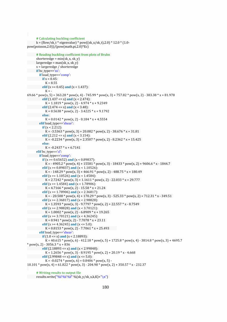
180

# Calculating buckling coefficient k = (flow/sk_t * eigenvalue) * pow((sk_x/sk_t),2.0) * 12.0 * (1.0-pow(poisson,2.0))/(pow(math.pi,2.0)*Ec) # Reading buckling coefficient from plots of Bruhn shorteredge = min(sk_x, sk_y) largeredge = max(sk_x, sk_y) x = largeredge / shorteredge if bc_type=='ss': if load_type=='comp': if x < 0.45: K = 8.55 elif (x >= 0.45) and (x < 1.437): K = -69.66 * pow(x, 5) + 363.28 * pow(x, 4) - 745.99 * pow(x, 3) + 757.82 * pow(x, 2) - 383.38 * x + 81.978 elif (1.437 <= x) and (x < 2.474): K = 1.1819 * pow(x, 2) - 4.974 * x + 9.2349 elif (2.474 <= x) and (x < 3.48): K = 0.5638 * pow(x, 2) - 3.4225 * x + 9.1792 else: K = 0.0142 * pow(x, 2) - 0.184 * x + 4.5554 elif load_type=='shear': if (x < 2.212): K = -3.5363 * pow(x, 3) + 20.082 * pow(x, 2) - 38.676 * x + 31.81 elif (2.212 <= x) and (x < 3.154): K = -0.2234 * pow(x, 3) + 2.3507 * pow(x, 2) - 8.2362 * x + 15.425 else: K = -0.2437 * x + 6.7141 elif bc_type=='cl': if load_type=='comp': if (x >= 0.65652) and (x < 0.89837): K = - 4905.2 * pow(x, 4) + 15581 * pow(x, 3) - 18433 * pow(x, 2) + 9606.6 * x - 1844.7 elif (x >= 0.89837) and (x < 1.10526): K = - 148.29 * pow(x, 3) + 466.91 * pow(x, 2) - 488.75 * x + 180.49 elif (x >= 1.10526) and (x < 1.4584): K = 2.7242 * pow(x, 3) + 1.1611 * pow(x, 2) - 22.033 * x + 29.777 elif (x >= 1.4584) and (x < 1.78906): K = 4.7166 * pow(x, 2) - 15.58 * x + 21.24 elif (x >= 1.78906) and (x < 2.36817): K = - 20.508 * pow(x, 4) + 170.29 * pow(x, 3) - 525.33 * pow(x, 2) + 712.31 * x - 349.51 elif (x >= 2.36817) and (x < 2.98828): K = 1.3593 * pow(x, 3) - 9.7797 * pow(x, 2) + 22.557 * x - 8.7549 elif (x >= 2.98828) and (x < 3.70121): K = 1.0002 * pow(x, 2) - 6.8909 * x + 19.265 elif (x >= 3.70121) and (x < 4.36245): K = 0.941 * pow(x, 2) - 7.7078 * x + 23.11 elif (x >= 4.36245) and (x <= 5.0): K = 0.8153 * pow(x, 2) - 7.7061 * x + 25.493 elif load_type=='shear': if (1.0 <= x) and (x < 2.18893): K = 40.615 * pow(x, 6) - 412.18 * pow(x, 5) + 1725.8 * pow(x, 4) - 3814.8 * pow(x, 3) + 4695.7 * pow(x, 2) - 3056.3 * x + 836 elif (2.18893 <= x) and (x < 2.99848): K = 1.2656 * pow(x, 3) - 8.9195 * pow(x, 2) + 20.19 * x - 4.668 elif (2.99848 <= x) and (x <= 5.0): K = -0.0274 * pow(x, 6) + 0.8406 * pow(x, 5) -10.101 * pow(x, 4) + 61.822 * pow(x, 3) - 204.98 * pow(x, 2) + 350.57 * x - 232.37 # Writing results to output file results.write("%f %f %f" %(sk_y/sk_x,k,K)+"\n")

181

results.close() try: del mdb.models['Model-1'] except: None # Saving the model mdb.saveAs( pathName=save_path+'.cae')

F.2 Linear Metal Stiffened Panel Buckling Python Scripts

• Example code to construct the skin-stringer model with J stringer section

# Importing necessary modules from part import * from material import * from section import * from assembly import * from step import * from interaction import * from load import * from mesh import * from optimization import * from job import * from sketch import * from visualization import * from connectorBehavior import * import math import time # Counter for script time start_t_time = time.time() # Paths save_path='C:/Users/……………………/Model/Model_J/model_j' # Initialize result file results = open(r"C:\Users\……………………\Results\output_J_min_inertia.txt","w+") # Given Edge Load (N/mm) Edge_load = 1.0 # Material properties (Al 2024 T3 Sheet thk: 0.23-3.25 mm) Ec = 73774.0 E = 72395.0 density = 2768.0 poisson = 0.33 Fcy = 269.0 nc = 15.0 # Skin geometry sk_x = 450.0 sk_ys = [150.0*3.0,225.0*3.0,300.0*3.0,375.0*3.0,450.0*3.0] sk_ts = [0.813,1.016,1.27] # Stringer "J" geometry str_l = 450.0 str_ts = [0.813,1.016,1.27] str_hs = [10.0,17.0,24.0,30.0]

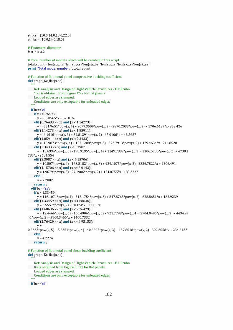
182

str_cs = [10.0,14.0,18.0,22.0] str_bs = [10.0,14.0,18.0] # Fasteners' diameter fast_d = 3.2 # Total number of models which will be created in this script total_count = len(str_hs)*len(str_cs)*len(str_bs)*len(str_ts)*len(sk_ts)*len(sk_ys) print "Total model number: ", total_count # Function of flat metal panel compressive buckling coefficient def graph_Kc_flat(x,bc): """ Ref: Analysis and Design of Flight Vehicle Structures - E.F.Bruhn * Kc is obtained from Figure C5.2 for flat panels Loaded edges are clamped. Conditions are only exceptable for unloaded edges """ if bc=='cl': if x < 0.76493: y = -56.0565*x + 57.1876 elif (0.76493 <= x) and (x < 1.14273): y = -551.9651*pow(x, 4) + 2079.3509*pow(x, 3) - 2870.2033*pow(x, 2) + 1706.6187*x- 353.426 elif (1.14273 <= x) and (x < 1.85911): y = -6.1616*pow(x, 3) + 34.8139*pow(x, 2) - 65.0106*x + 48.5687 elif (1.85911 <= x) and (x < 2.3433): y = -15.9873*pow(x, 4) + 127.1208*pow(x, 3) - 373.7913*pow(x, 2) + 479.4634*x - 216.8528 elif (2.3433 <= x) and (x < 3.3987): y = 13.6994*pow(x, 5) - 198.9195*pow(x, 4) + 1149.7887*pow(x, 3) - 3306.5735*pow(x, 2) + 4730.1783*x - 2684.554 elif (3.3987 <= x) and (x < 4.15706): y = 10.807*pow(x, 4) - 163.8182*pow(x, 3) + 929.1075*pow(x, 2) - 2336.7822*x + 2206.491 elif (4.15706 <= x) and (x <= 5.0142): y = 1.9679*pow(x, 3) - 27.1906*pow(x, 2) + 124.8755*x - 183.3227 else: y = 7.2802 return y elif bc=='ss': if x < 1.33459: y = 116.1071*pow(x, 4) - 512.1754*pow(x, 3) + 847.8765*pow(x, 2) - 628.8651*x + 183.9239 elif (1.33459 <= x) and (x < 1.68636): y = 2.5557*pow(x, 2) - 8.0374*x + 11.8528 elif (1.68636 <= x) and (x < 2.76429): y = 12.4466*pow(x, 6) - 166.4906*pow(x, 5) + 921.7798*pow(x, 4) - 2704.0495*pow(x, 3) + 4434.9741*pow(x, 2) - 3860.3466*x + 1400.7332 elif (2.76429 <= x) and (x <= 4.95153): y = -0.2663*pow(x, 5) + 5.2351*pow(x, 4) - 40.8202*pow(x, 3) + 157.8018*pow(x, 2) - 302.6058*x + 234.8432 else: y = 4.2274 return y # Function of flat metal panel shear buckling coefficient def graph_Ks_flat(x,bc): """ Ref: Analysis and Design of Flight Vehicle Structures - E.F.Bruhn Ks is obtained from Figure C5.11 for flat panels Loaded edges are clamped. Conditions are only exceptable for unloaded edges """ if bc=='cl':

183

if x < 1.39646: y = 617.3722*pow(x, 4) - 3049.2054*pow(x, 3) + 5640.7618*pow(x, 2) - 4637.94*x + 1444.5082 elif (1.39646 <= x) and (x < 2.79647): y = -0.2876*pow(x, 3) + 3.08*pow(x, 2) - 10.558*x + 21.4866 elif (2.79647 <= x) and (x < 5.0): y = 0.2326*pow(x, 5) - 4.577*pow(x, 4) + 35.6865*pow(x, 3) - 137.6532*pow(x, 2) + 262.3421*x - 187.6865 else: y = 9.6226 return y elif bc=='ss': if x < 1.79125: y = -23.165*pow(x, 6) + 154.3269*pow(x, 5) - 380.7138*pow(x, 4) + 376.5476*pow(x, 3) - 1.3356*pow(x, 2) - 251.0012*x + 135.069 elif (x <= 1.79125) and (x < 2.57994): y = 0.1192*pow(x, 3) - 0.7131*pow(x, 2) + 0.5982*x + 7.1608 elif (x <= 2.57994) and (x < 3.70882): y = 0.075*pow(x, 3) - 0.3925*pow(x, 2) + 0.0756*x + 7.135 elif (x <= 3.70882) and (x < 5.0): y = -0.2125*x + 6.6311 else: y = 5.5684 return y # Function of plasticity correction def get_plastic_stress(nc,Fscr_el,Ec,Fcy): """ See HSB 52100-01 plasticity correction """ return Fcr for sk_y_key,sk_y in enumerate(sk_ys): for sk_t_key,sk_t in enumerate(sk_ts): sk_ratio = sk_x / (sk_y/3.0) Ireqs =[] K_values =[] # Unloaded edge boundary conditions (clamped or simply supported) for bc in ["cl","ss"]: Ks = graph_Ks_flat(sk_ratio,bc) Kc = graph_Kc_flat(sk_ratio,bc) K_value = [Ks,Kc] K_values.append(K_value) Fscr_el = Ks*math.pi**2.0*Ec/(12.0*(1.0-poisson**2.0))*(sk_t/(sk_y/3.0))**2.0 Fscr = get_plastic_stress(nc,Fscr_el,Ec,Fcy) Ireq = (2.29*sk_x/sk_t)*(Fscr*sk_t*((sk_y/3.0)**2.0)/(33.0*E))**(4.0/3.0) Ireqs.append(Ireq) Ireq_moi=min(Ireqs) # Results of panels with classical boundary conditions and minimum required inertia are written into the result file results.write("%-15s %6.2f %-15s %6.2f" %("Skin length y: ",(sk_y/3.0)," Skin thickness: ",sk_t)+"\n") results.write("%-30s %-15s %6.2f %-30s %6.2f" %("Min. stiffener inertia" ,"For clamped: ",Ireqs[0]," For simply supported",Ireqs[1])+"\n") results.write("%-30s %-15s %6.2f %-30s %6.2f" %("Shear buckling coeffient" ,"For clamped: ",K_values[0][0]," For simply supported",K_values[1][0])+"\n")

184

results.write("%-30s %-15s %6.2f %-30s %6.2f" %("Compressive buckling coeffient" ,"For clamped: ",K_values[0][1]," For simply supported",K_values[1][1])+"\n"+"\n") for str_h_key,str_h in enumerate(str_hs): for str_c_key,str_c in enumerate(str_cs): for str_b_key,str_b in enumerate(str_bs): for str_t_key,str_t in enumerate(str_ts): # Inertia and area of stringer is calculated r1_dx = str_b r1_dy = str_t r2_dx = str_t r2_dy = str_h-2.0*str_t r3_dx = str_c r3_dy = str_t r1_A = r1_dx * r1_dy r2_A = r2_dx * r2_dy r3_A = r3_dx * r3_dy r1_Ix = (1.0 / 12.0) * r1_dx * r1_dy**3.0 r2_Ix = (1.0 / 12.0) * r2_dx * r2_dy**3.0 r3_Ix = (1.0 / 12.0) * r3_dx * r3_dy**3.0 parts = [ {'dx_cg': max(r1_dx-r2_dx/2.0,r3_dx/2.0) + r2_dx/2.0 - r1_dx/2.0, 'dy_cg': r1_dy / 2.0, 'A':r1_A, 'Ix':r1_Ix}, {'dx_cg': max(r1_dx-r2_dx/2.0,r3_dx/2.0), 'dy_cg': r1_dy + r2_dy / 2.0, 'A':r2_A, 'Ix':r2_Ix}, {'dx_cg': max(r1_dx-r2_dx/2.0,r3_dx/2.0), 'dy_cg': r1_dy + r2_dy + r3_dy / 2.0, 'A':r3_A, 'Ix':r3_Ix}, ] Ad_t = 0.0 A_t = 0.0 for part in parts: Ad_t += part['A'] * part['dy_cg'] A_t += part['A'] cg_y = Ad_t / A_t Istr = 0.0 for part in parts: Istr += (part['Ix'] + part['A'] * part['dy_cg']** 2.0 - cg_y * part['A'] * part['dy_cg']) # Geometric properties of stringer are written into the result file results.write("%-25s %6.2f %-20s %6.2f %-20s %6.2f %-20s %6.2f" %(" Stringer heigth: ",str_h, " Stringer c width: ",str_c, " Stringer b width: ",str_b," Stringer thickness: ",str_t)+"\n") results.write("%-25s %6.2f" %(" Stiffener inertia: ",Istr)+"\n"+"\n") # To satisfy the stiffened panel condition, stringer inertia is checked. if Ireq_moi<Istr: # Creating model of stiffened panel buckling (spb) model_name = "spb_J_"+str(str_h_key)+str(str_c_key)+str(str_b_key)+str(str_t_key)+str(sk_t_key)+str(sk_y_key) mdb.Model(modelType=STANDARD_EXPLICIT, name=model_name) mn=mdb.models[model_name] # Creating material mn.Material(name='Al_2024_T3_Sheet') mn.materials['Al_2024_T3_Sheet'].Elastic(table=((Ec, poisson), )) mn.materials['Al_2024_T3_Sheet'].Density(table=((density, ), )) # Creating sketch of skin mn.ConstrainedSketch(name='__profile__', sheetSize=200.0) mn.sketches['__profile__'].rectangle(point1=(0.0, 0.0), point2=(sk_x, sk_y))

185

# Creating part of skin mn.Part(dimensionality=THREE_D, name='Skin', type=DEFORMABLE_BODY) mn.parts['Skin'].BaseShell(sketch=mn.sketches['__profile__']) del mn.sketches['__profile__'] # Creating partition p_sk = mn.parts['Skin'] f_sk, e_sk, d_sk = p_sk.faces, p_sk.edges, p_sk.datums t = p_sk.MakeSketchTransform(sketchPlane=f_sk[0], sketchUpEdge=e_sk[2], sketchPlaneSide=SIDE1, origin=(sk_x*0.5, sk_y*0.5, 0.0)) s = mn.ConstrainedSketch(name='__profile__', sheetSize=1272.79, gridSpacing=31.81, transform=t) g, v, d1, c = s.geometry, s.vertices, s.dimensions, s.constraints s.setPrimaryObject(option=SUPERIMPOSE) p_sk.projectReferencesOntoSketch(sketch=s, filter=COPLANAR_EDGES) s.Line(point1=(-sk_y/6.0, sk_x*0.5), point2=(-sk_y/6.0, -sk_x*0.5)) s.VerticalConstraint(entity=g[6], addUndoState=False) s.PerpendicularConstraint(entity1=g[5], entity2=g[6], addUndoState=False) s.CoincidentConstraint(entity1=v[4], entity2=g[5], addUndoState=False) s.CoincidentConstraint(entity1=v[5], entity2=g[3], addUndoState=False) s.Line(point1=(0, sk_x*0.5), point2=(0, -sk_x*0.5)) s.VerticalConstraint(entity=g[7], addUndoState=False) s.PerpendicularConstraint(entity1=g[5], entity2=g[7], addUndoState=False) s.CoincidentConstraint(entity1=v[6], entity2=g[5], addUndoState=False) s.CoincidentConstraint(entity1=v[7], entity2=g[3], addUndoState=False) s.Line(point1=(sk_y/6.0, sk_x*0.5), point2=(sk_y/6.0, -sk_x*0.5)) s.VerticalConstraint(entity=g[8], addUndoState=False) s.PerpendicularConstraint(entity1=g[5], entity2=g[8], addUndoState=False) s.CoincidentConstraint(entity1=v[8], entity2=g[5], addUndoState=False) s.CoincidentConstraint(entity1=v[9], entity2=g[3], addUndoState=False) pickedFaces = f_sk.getSequenceFromMask(mask=('[#1 ]', ), ) p_sk.PartitionFaceBySketch(sketchUpEdge=e_sk[2], faces=pickedFaces, sketch=s) s.unsetPrimaryObject() del mn.sketches['__profile__'] # Creating skin section mn.HomogeneousShellSection(name='Skin_Sec', preIntegrate=OFF, material='Al_2024_T3_Sheet', thicknessType=UNIFORM, thickness=sk_t, thicknessField='', idealization=NO_IDEALIZATION, poissonDefinition=DEFAULT, thicknessModulus=None, temperature=GRADIENT, useDensity=OFF, integrationRule=SIMPSON, numIntPts=5) # Assigning skin section faces = f_sk.getSequenceFromMask(mask=('[#f ]', ), ) region = p_sk.Set(faces=faces, name='Skin_faces_set') p_sk.SectionAssignment(region=region, sectionName='Skin_Sec', offset=0.0, offsetType=MIDDLE_SURFACE, offsetField='', thicknessAssignment=FROM_SECTION) # Mesh control of skin pickedRegions = f_sk.getSequenceFromMask(mask=('[#f ]', ), ) p_sk.setMeshControls(regions=pickedRegions, elemShape=QUAD, technique=SWEEP) # Mesh seed of skin p_sk.seedPart(deviationFactor=0.1, minSizeFactor=0.1, size=5.0) # Generate mesh of skin p_sk.generateMesh() # Creating sketch of stringer

186

s = mn.ConstrainedSketch(name='__profile__', sheetSize=200.0) g, v, d, c = s.geometry, s.vertices, s.dimensions, s.constraints s.setPrimaryObject(option=STANDALONE) s.Line(point1=(-str_c*0.5, 0.0), point2=(str_c*0.5, 0.0)) s.HorizontalConstraint(entity=g[2], addUndoState=False) s.Line(point1=(0.0, 0.0), point2=(0.0, str_h)) s.VerticalConstraint(entity=g[3], addUndoState=False) s.PerpendicularConstraint(entity1=g[2], entity2=g[3], addUndoState=False) s.CoincidentConstraint(entity1=v[2], entity2=g[2], addUndoState=False) s.EqualDistanceConstraint(entity1=v[0], entity2=v[1], midpoint=v[2], addUndoState=False) s.Line(point1=(0.0, str_h), point2=(str_b, str_h)) s.HorizontalConstraint(entity=g[4], addUndoState=False) s.PerpendicularConstraint(entity1=g[3], entity2=g[4], addUndoState=False) # Creating part of stringer mn.Part(name='Stringer', dimensionality=THREE_D,type=DEFORMABLE_BODY) mn.parts['Stringer'].BaseShellExtrude(sketch=s, depth=str_l) del mn.sketches['__profile__'] # Creating stringer section mn.HomogeneousShellSection(name='Stringer_Sec', preIntegrate=OFF, material='Al_2024_T3_Sheet', thicknessType=UNIFORM, thickness=str_t, thicknessField='', idealization=NO_IDEALIZATION, poissonDefinition=DEFAULT, thicknessModulus=None, temperature=GRADIENT, useDensity=OFF, integrationRule=SIMPSON, numIntPts=5) # Assigning stringer section p_str = mn.parts['Stringer'] f_str = p_str.faces faces = f_str.getSequenceFromMask(mask=('[#f ]', ), ) region = p_str.Set(faces=faces, name='Stringer_faces_set') p_str.SectionAssignment(region=region, sectionName='Stringer_Sec', offset=0.0, offsetType=MIDDLE_SURFACE, offsetField='', thicknessAssignment=FROM_SECTION) # Mesh control of stringer pickedRegions = f_str.getSequenceFromMask(mask=('[#f ]', ), ) p_str.setMeshControls(regions=pickedRegions, elemShape=QUAD, technique=SWEEP) # Mesh seed of stringer p_str.seedPart(deviationFactor=0.1, minSizeFactor=0.1, size=2.0) # Generate mesh of stringer p_str.generateMesh() # Creating buckling step mn.BuckleStep(name='Buckle-Step', previous='Initial', numEigen=3, vectors=28, maxIterations=3000) # Creating assembly instances a_ss = mn.rootAssembly a_ss.DatumCsysByDefault(CARTESIAN) a_ss.Instance(dependent=ON, name='Skin-1', part=p_sk) # Creating Stringer 1 mn.rootAssembly.DatumCsysByDefault(CARTESIAN) mn.rootAssembly.Instance(dependent=ON, name='Stringer-1', part=p_str) # Stringer 1 place is decided

187

a_ss.rotate(instanceList=('Stringer-1', ), axisPoint=(0.0, 0.0, 0.0), axisDirection=(0.0, 1.0, 0.0), angle=90.0) a_ss.rotate(instanceList=('Stringer-1', ), axisPoint=(0.0, 0.0, 0.0), axisDirection=(1.0, 0.0, 0.0), angle=90.0) a_ss.translate(instanceList=('Stringer-1', ), vector=(0.0, sk_y/3.0, (sk_t+str_t)*0.5)) # Creating Stringer 2 a_ss.LinearInstancePattern(instanceList=('Stringer-1', ), direction1=(1.0, 0.0, 0.0), direction2=(0.0, 1.0, 0.0), number1=1, number2=2, spacing1=str_l, spacing2=sk_y/3.0) a_ss.features.changeKey(fromName='Stringer-1-lin-1-2', toName='Stringer-2') # Creating Connector section as beam mn.ConnectorSection(name='Fastener_Con_Sec', assembledType=BEAM) # Creating Fasteners const_attach = [['[#20 ]',4,1,'1'],['[#4 ]',2,0,'2']] for key in range(2): e_str = a_ss.instances['Stringer-'+str(key+1)].edges v_str = a_ss.instances['Stringer-'+str(key+1)].vertices f_str = a_ss.instances['Stringer-'+str(key+1)].faces for const in const_attach: # Creating attachment points edges1 = e_str.getSequenceFromMask(mask=(const[0], ), ) geomEdges=edges1 a_ss.AttachmentPointsOffsetFromEdges(edges=geomEdges, startPoint=v_str[const[1]], referenceFace=f_str[const[2]], name='Str'+str(key+1)+'-Attachment Points-'+const[3], pointCreationMethod=BY_NUMBER, offsetFromStartPoint=2.0*fast_d+1.0, numberOfPoints=27, offsetFromEndPoint=2.0*fast_d+1.0, numberOfRows=1, offsetFromEdges= str_c*0.25, patterningMethod=PATTERN_ORTHOGONALLY, setName='Str'+str(key+1)+'-Attachment Points-Set '+const[3]) # Assigning a section to fastener region=a_ss.sets['Str'+str(key+1)+'-Attachment Points-Set '+const[3]] a_ss.engineeringFeatures.PointFastener( name='Str'+str(key+1)+'-Fasteners-'+const[3], region=region, sectionName='Fastener_Con_Sec', directionVector=(v_str[7], a_ss.instances['Stringer-'+str(key+1)]. InterestingPoint(edge=e_str[8], rule=MIDDLE)), physicalRadius=fast_d*0.5, additionalMass=0.0001) # Creating boundary conditions at initial step v_sk = a_ss.instances['Skin-1'].vertices e_sk = a_ss.instances['Skin-1'].edges #Creating boundary conditions sets verts1 = v_sk.getSequenceFromMask(mask=('[#200 ]', ), ) a_ss.Set(vertices=verts1, name='Set_mid_point') dict_bc = {'[#44 ]':'side_edges','[#c28 ]':'load_edge','[#1282 ]':'reaction_edge',} for key_bc,str_bc in dict_bc.items(): edges1 = e_sk.getSequenceFromMask(mask=(key_bc, ), ) a_ss.Set(edges=edges1, name='Set_'+str_bc) # Assigning boundary conditions on sets region = a_ss.sets['Set_mid_point'] mn.DisplacementBC(name='BC_mid_point', createStepName='Initial', region=region, u1=UNSET, u2=SET, u3=UNSET, ur1=UNSET, ur2=UNSET, ur3=UNSET, amplitude=UNSET, distributionType=UNIFORM,

188

fieldName='', localCsys=None) region = a_ss.sets['Set_side_edges'] mn.DisplacementBC(name='BC_side_edges', createStepName='Initial', region=region, u1=UNSET, u2=UNSET, u3=SET, ur1=SET, ur2=UNSET, ur3=UNSET, amplitude=UNSET, distributionType=UNIFORM, fieldName='', localCsys=None) region = a_ss.sets['Set_load_edge'] mn.DisplacementBC(name='BC_load_edge', createStepName='Initial', region=region, u1=UNSET, u2=UNSET, u3=SET, ur1=UNSET, ur2=SET, ur3=UNSET, amplitude=UNSET, distributionType=UNIFORM, fieldName='', localCsys=None) region = a_ss.sets['Set_reaction_edge'] mn.DisplacementBC(name='BC_reaction_edge', createStepName='Initial', region=region, u1=SET, u2=UNSET, u3=SET, ur1=UNSET, ur2=SET, ur3=UNSET, amplitude=UNSET, distributionType=UNIFORM, fieldName='', localCsys=None) # Creating shell edge load loaded_edges = e_sk.getSequenceFromMask(mask=('[#c28 ]', ), ) region = a_ss.Surface(side1Edges=loaded_edges, name='Loaded Edge Surface') mn.ShellEdgeLoad(name='Shell Load', createStepName='Buckle-Step', region=region, magnitude=Edge_load, distributionType=UNIFORM, field='', localCsys=None) # Creating job job_name ='job_'+ model_name mdb.Job(name=job_name, model=model_name, description='', type=ANALYSIS, atTime=None, waitMinutes=0, waitHours=0, queue=None, memory=99, memoryUnits=PERCENTAGE, getMemoryFromAnalysis=True, explicitPrecision=SINGLE, nodalOutputPrecision=SINGLE, echoPrint=OFF, modelPrint=OFF, contactPrint=OFF, historyPrint=OFF, userSubroutine='', scratch='', resultsFormat=ODB, multiprocessingMode=DEFAULT, numCpus=1, numGPUs=0) results.close() del mdb.models['Model-1'] # Saving the model mdb.saveAs(pathName=save_path+'.cae') # Stoping the time calculater end_t_time = time.time() m=divmod(end_t_time-start_t_time,60) n=divmod(m[0],60) print "Total time: " ,n[0],n[1],m[1]

• Example code to process finite element results for skin-stringer model with J

stringer section

# Importing necessary modules from part import * from material import * from section import * from assembly import * from step import * from interaction import * from load import * from mesh import * from optimization import * from job import *

189

from sketch import * from visualization import * from connectorBehavior import * import math import time # Counter for script time start_t_time = time.time() # Defining maximum number of submittions can be given at the same time max_sub = 5 ini_sub = 0 # Paths save_path = 'C:/Users/……………………/Model/Model_J/model_j' model_path = r'C:/Users/Enes/Desktop/AIAC/Versions/V7/Model/Model_J/' # Initialize result files results = open(r"C:\Users\……………………\Results\output_J.txt","w+") results_excel = open(r"C:\Users\……………………\Results\excel_output_J.txt","w+") # Given Edge Load (N/mm) Edge_load = 1.0 # Material properties (Al 2024 T3 Sheet thk: 0.23-3.25 mm) Ec = 73774.0 E = 72395.0 density = 2768.0 poisson = 0.33 Fcy = 269.0 nc = 15.0 # Skin geometry sk_x = 450.0 sk_ys = [150.0*3.0,225.0*3.0,300.0*3.0,375.0*3.0,450.0*3.0] sk_ts = [0.813,1.016,1.27] # Stringer "J" geometry str_l = 450.0 str_ts = [0.813,1.016,1.27] str_hs = [10.0,17.0,24.0,30.0] str_cs = [10.0,14.0,18.0,22.0] str_bs = [10.0,14.0,18.0] # Fasteners' diameter fast_d = 3.2 # Initialize output file results.write("%-20s %6.0f %-20s %6.2f %-20s %6.2f" %("Material Ec: ",Ec," Material poisson: ",poisson," Material density: ",density)+"\n") results.write("%-20s %6.2f %-20s %6.2f %-20s %6.2f" %("Skin length x: ",sk_x," Stringer length: ",str_l," Fastener diameter: ",fast_d)+"\n"+"\n") # Total number of models which will be created in this script total_count = len(str_hs)*len(str_cs)*len(str_bs)*len(str_ts)*len(sk_ts)*len(sk_ys) print "Total model number: ", total_count count=1 # Initialize dictionary for excel output file excel_dic = {"Skin_length_y":[],"Skin_thickness":[],"Stringer_heigth":[],"Stringer_c_width":[],"Stringer_b_width":[],"Stringer_thickness":[],"kc":[]}

190

# Function of flat metal panel compressive buckling coefficient def graph_Kc_flat(x,bc): """ Ref: Analysis and Design of Flight Vehicle Structures - E.F.Bruhn Kc is obtained from Figure C5.2 for flat panels Loaded edges are clamped. Conditions are only exceptable for unloaded edges """ if bc=='cl': if x < 0.76493: y = -56.0565*x + 57.1876 elif (0.76493 <= x) and (x < 1.14273): y = -551.9651*pow(x, 4) + 2079.3509*pow(x, 3) - 2870.2033*pow(x, 2) + 1706.6187*x- 353.426 elif (1.14273 <= x) and (x < 1.85911): y = -6.1616*pow(x, 3) + 34.8139*pow(x, 2) - 65.0106*x + 48.5687 elif (1.85911 <= x) and (x < 2.3433): y = -15.9873*pow(x, 4) + 127.1208*pow(x, 3) - 373.7913*pow(x, 2) + 479.4634*x - 216.8528 elif (2.3433 <= x) and (x < 3.3987): y = 13.6994*pow(x, 5) - 198.9195*pow(x, 4) + 1149.7887*pow(x, 3) - 3306.5735*pow(x, 2) + 4730.1783*x - 2684.554 elif (3.3987 <= x) and (x < 4.15706): y = 10.807*pow(x, 4) - 163.8182*pow(x, 3) + 929.1075*pow(x, 2) - 2336.7822*x + 2206.491 elif (4.15706 <= x) and (x <= 5.0142): y = 1.9679*pow(x, 3) - 27.1906*pow(x, 2) + 124.8755*x - 183.3227 else: y = 7.2802 return y elif bc=='ss': if x < 1.33459: y = 116.1071*pow(x, 4) - 512.1754*pow(x, 3) + 847.8765*pow(x, 2) - 628.8651*x + 183.9239 elif (1.33459 <= x) and (x < 1.68636): y = 2.5557*pow(x, 2) - 8.0374*x + 11.8528 elif (1.68636 <= x) and (x < 2.76429): y = 12.4466*pow(x, 6) - 166.4906*pow(x, 5) + 921.7798*pow(x, 4) - 2704.0495*pow(x, 3) + 4434.9741*pow(x, 2) - 3860.3466*x + 1400.7332 elif (2.76429 <= x) and (x <= 4.95153): y = -0.2663*pow(x, 5) + 5.2351*pow(x, 4) - 40.8202*pow(x, 3) + 157.8018*pow(x, 2) - 302.6058*x + 234.8432 else: y = 4.2274 return y for sk_y_key,sk_y in enumerate(sk_ys): for sk_t_key,sk_t in enumerate(sk_ts): for str_h_key,str_h in enumerate(str_hs): for str_c_key,str_c in enumerate(str_cs): for str_b_key,str_b in enumerate(str_bs): for str_t_key,str_t in enumerate(str_ts): # Job name is described job_name = "job_spb_J_"+str(str_h_key)+str(str_c_key)+str(str_b_key)+str(str_t_key)+str(sk_t_key)+str(sk_y_key) # Checked whether there is such a job name try: start_time = time.time() print "Model number: ",count job_model = mdb.jobs[job_name] # Checked to see if the job has already been submitted try:

191

dir_logfile = model_path + job_name+".log" logfile = open(dir_logfile) comp = False # Checked to see that the job is completed for line in logfile: if "Abaqus JOB "+job_name+" COMPLETED" in line: print " completed" comp = True logfile.close() # Submittion check if comp==False: # Submit the job job_model.submit(consistencyChecking=OFF) ini_sub +=1 # Multi-submittion is permitted for this code # Maximum number of submittion is checked if ini_sub >= max_sub: job_model.waitForCompletion() ini_sub = 0 end_time = time.time() else: end_time = time.time() except: # Submit the job job_model.submit(consistencyChecking=OFF) ini_sub +=1 # Multi-submittion is permitted for this code # Maximum number of submittion is checked if ini_sub >= max_sub: job_model.waitForCompletion() ini_sub = 0 end_time = time.time() # Estimated time is calculated if count%(max_sub*2) == 0: em=divmod((total_count-count)*(end_time-start_time)/max_sub,60) en=divmod(em[0],60) print "Estimated remaning time: " ,en[0],en[1],em[1] count+=1 except: None for sk_y_key,sk_y in enumerate(sk_ys): sk_ratio = sk_x / (sk_y/3.0) kc_bruhn =[] # Literature graphs are used to get comp. buckling coeffients with classical boundary condition assumption # Unloaded edge boundary conditions (clamped or simply supported) for bc in ["cl","ss"]: kc_bruhn.append(graph_Kc_flat(sk_ratio,bc)) for sk_t_key,sk_t in enumerate(sk_ts): for str_h_key,str_h in enumerate(str_hs): for str_c_key,str_c in enumerate(str_cs): for str_b_key,str_b in enumerate(str_bs): for str_t_key,str_t in enumerate(str_ts): # Defining the job name

192

job_name = "job_spb_J_"+str(str_h_key)+str(str_c_key)+str(str_b_key)+str(str_t_key)+str(sk_t_key)+str(sk_y_key) # Obtain the eigenvalue try: dir_datfile = model_path + job_name+'.dat' wordlist = [] starttorecord = False datfile = open(dir_datfile) for line in datfile: if " MODE NO EIGENVALUE" in line: starttorecord = True for word in line.split(): if word=='THE': starttorecord = False if starttorecord: wordlist.append(word) if float(wordlist[4])>0.0: eigenvalue = float(wordlist[4]) elif float(wordlist[6])>0.0: eigenvalue = float(wordlist[6]) elif float(wordlist[8])>0.0: eigenvalue = float(wordlist[8]) else: eigenvalue = 0.0 datfile.close() Fccr=eigenvalue*Edge_load/sk_t # Compressive buckling coeffient is calculated using eigenvalue obtained from FEA kc=Fccr*(sk_y/3.0)**2.0*12.0*(1.0-poisson**2.0)/(Ec*(math.pi*sk_t)**2.0) kc_star=kc*math.pi**2.0/(12.0*(1.0-poisson**2.0)) # Write the excel data excel_dic["Skin_length_y"].append(sk_y/3.0) excel_dic["Skin_thickness"].append(sk_t) excel_dic["Stringer_heigth"].append(str_h) excel_dic["Stringer_c_width"].append(str_c) excel_dic["Stringer_b_width"].append(str_b) excel_dic["Stringer_thickness"].append(str_t) excel_dic["kc"].append(kc) # Write the input data results.write("%-25s %6.2f %-20s %6.2f %-20s %6.2f %-20s %6.2f %-20s %6.2f %-20s %6.2f" %(" Skin length y: ",(sk_y/3.0)," Skin thickness: ",sk_t," Stringer heigth: ",str_h," Stringer c width: ",str_c," Stringer b width: ",str_b," Stringer thickness: ",str_t)+"\n") # Write the output data results.write("%-25s %6.2f %-20s %6.2f %-20s %6.2f" %(" Eigenvalue: ",eigenvalue," Fccr: ",Fccr," kc_star: ",kc_star)+"\n") results.write("%-25s %6.3f %-20s %6.3f %-20s %6.3f" %(" kc: ",kc," Bruhn kc(clamped): ",kc_bruhn[0]," Bruhn kc(ss): ",kc_bruhn[1])+"\n"+"\n") except: None # Excel output results are written into the output file for excel_key,excel_data in excel_dic.items(): results_excel.write("%-20s"%(excel_key)) for excel_var in excel_data: results_excel.write("%8.2f"%(excel_var)) results_excel.write("\n") if excel_key=="kc": results_excel.write("\n")

193

results.close() results_excel.close() # Saving the model mdb.saveAs(pathName=save_path+'.cae') # Stoping the time calculater end_t_time = time.time() m=divmod(end_t_time-start_t_time,60) n=divmod(m[0],60) print "Total time: " ,n[0],n[1],m[1]

F.3 ANN Matlab Script

% Clearing the workspace and command window clc; clear all; close all; warning('off','MATLAB:xlswrite:AddSheet'); % Interval of ANN parameters which is tried to get max. performance in ANN. % Order T,Z,J % neurons = {[6],[6],[8]}; % ratios = {{[70,20,10]},{[90,5,5]},{[70,15,15]}}; types = ['T','Z','J']; neurons = {[10],[10],[10]}; ratios = {{[70,20,10],[70,15,15],[75,15,10]}, ... {[70,20,10],[70,15,15],[75,15,10]},... {[70,20,10],[70,15,15],[75,15,10]}}; trials = 10; t_n= length(neurons{1})*length(types)*length(ratios{1})*trials; t_n_disp = sprintf('Total number of iteration : %d',t_n); disp(t_n_disp) i_n=1; for ii=1:1:length(types); type=types(ii); str_type_disp = sprintf('Stringer type : %s',type); disp(str_type_disp) % Opening excel file to read ANN database inputs, additional ten sample % cases input and output values data = xlsread('ANN_abaqus.xlsx',strcat('Data_',type)); sample = xlsread('ANN_abaqus.xlsx',strcat('Sample_',type)); fem_output = xlsread('ANN_abaqus.xlsx',... strcat('Sample_Results_',type),'B1:K1'); % Input matrix is rearranged. num_data = size(data,1); for kk=3:1:num_data; input(kk-2,:)=data(kk,:); end target = data(1,:); for nn=1:1:length(neurons{ii}); neuron = neurons{ii}(nn); pre_rse = 1.0; for rr=1:1:length(ratios{ii}); ratio = ratios{ii}{rr}; for ss=1:1:trials; network = fitnet(neuron);

194

network.inputs{1}.processFcns = {'removeconstantrows',... 'mapminmax'}; network.outputs{2}.processFcns = {'removeconstantrows',... 'mapminmax'}; network.divideFcn = 'dividerand'; network.divideMode = 'sample'; % Configuring the ANN parameters to use in training itself network.divideParam.trainRatio = ratio(1)/100; network.divideParam.valRatio = ratio(2)/100; network.divideParam.testRatio = ratio(3)/100; network.trainFcn = 'trainlm'; network.performFcn = 'mse'; % Parameters can be changed after the training method % described ('trainlm') network.trainParam.max_fail = 500; network.trainParam.epochs = 1500; network.plotFcns = {'plotperform','plottrainstate',... 'ploterrhist', 'plotregression','plotfit'}; [network,tr] = train(network,input,target); % ANN results, errors and performance values are stored. output = network(input); error = gsubtract(target,output); performance = perform (network,target,output); % Target input values are stored to calculate performances % of ANN. trainTargets = target .* tr.trainMask{1}; valTargets = target .* tr.valMask{1}; testTargets = target .* tr.testMask{1}; % ANN performances are calculated. trainPerformance = perform(network,trainTargets,output); valPerformance = perform(network,valTargets,output); testPerformance = perform(network,testTargets,output); % Root square error is calculated according to results of % additional ten FE analyses. sample_output = network(sample) ; square_error = 0; for ff=1:1:length(fem_output); square_error=square_error+(fem_output(ff)- ... sample_output(ff))^2; end rse = (square_error/length(fem_output))^0.5; % If the previous root square error is greater than current % calculated value, current ANN paramters are saved to % workspace. if pre_rse>rse; % Creating the performance plot and % then saving the plot plotperform(tr); saveas(gcf,strcat('perf_',type,'.png')); % Creating the training state values plot and % then saving the plot plottrainstate(tr) saveas(gcf,strcat('trn_',type,'.png'));

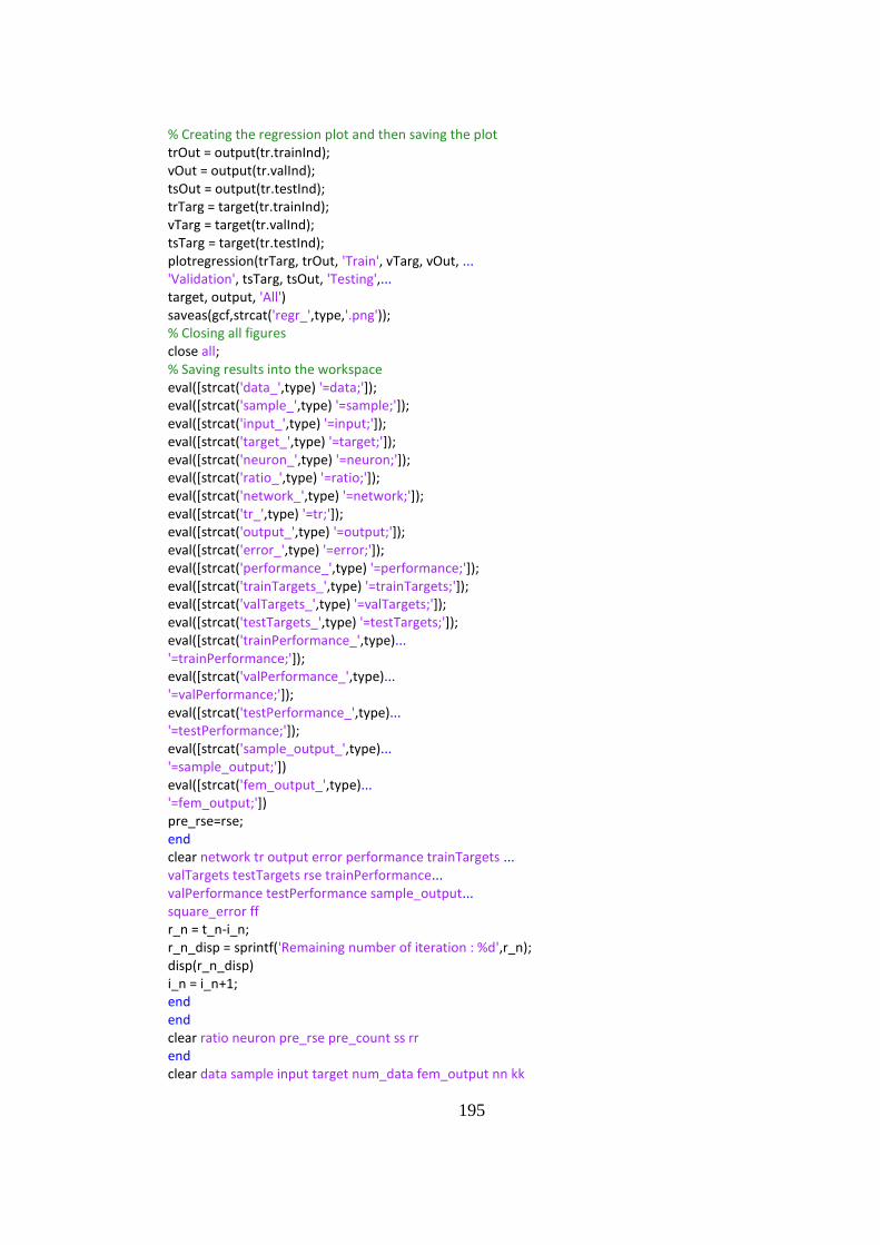
195

% Creating the regression plot and then saving the plot trOut = output(tr.trainInd); vOut = output(tr.valInd); tsOut = output(tr.testInd); trTarg = target(tr.trainInd); vTarg = target(tr.valInd); tsTarg = target(tr.testInd); plotregression(trTarg, trOut, 'Train', vTarg, vOut, ... 'Validation', tsTarg, tsOut, 'Testing',... target, output, 'All') saveas(gcf,strcat('regr_',type,'.png')); % Closing all figures close all; % Saving results into the workspace eval([strcat('data_',type) '=data;']); eval([strcat('sample_',type) '=sample;']); eval([strcat('input_',type) '=input;']); eval([strcat('target_',type) '=target;']); eval([strcat('neuron_',type) '=neuron;']); eval([strcat('ratio_',type) '=ratio;']); eval([strcat('network_',type) '=network;']); eval([strcat('tr_',type) '=tr;']); eval([strcat('output_',type) '=output;']); eval([strcat('error_',type) '=error;']); eval([strcat('performance_',type) '=performance;']); eval([strcat('trainTargets_',type) '=trainTargets;']); eval([strcat('valTargets_',type) '=valTargets;']); eval([strcat('testTargets_',type) '=testTargets;']); eval([strcat('trainPerformance_',type)... '=trainPerformance;']); eval([strcat('valPerformance_',type)... '=valPerformance;']); eval([strcat('testPerformance_',type)... '=testPerformance;']); eval([strcat('sample_output_',type)... '=sample_output;']) eval([strcat('fem_output_',type)... '=fem_output;']) pre_rse=rse; end clear network tr output error performance trainTargets ... valTargets testTargets rse trainPerformance... valPerformance testPerformance sample_output... square_error ff r_n = t_n-i_n; r_n_disp = sprintf('Remaining number of iteration : %d',r_n); disp(r_n_disp) i_n = i_n+1; end end clear ratio neuron pre_rse pre_count ss rr end clear data sample input target num_data fem_output nn kk

196

% Final reslts of additional ten analyses are written into the excel % file. sample_output_tmp = eval(strcat('sample_output_',type)); for ee=1:1:length(sample_output_tmp); range=sprintf('%c','A'+ee,'3'); xlswrite('ANN_abaqus.xlsx',sample_output_tmp(ee),... strcat('Sample_Results_',type), range); end clear range sample_output_tmp ee type end clear ii i_n r_n t_n % Saving the ANN workspace. save ANN_workspace.mat; % Opening the excel file. winopen('ANN_abaqus.xlsx'); disp('Calculation is over');

F.4 Metal Stiffened Panel Post-Buckling Python Scripts

• Example code to construct the skin-stringer model with I stringer section

# Importing necessary modules from part import * from material import * from section import * from assembly import * from step import * from interaction import * from load import * from mesh import * from optimization import * from job import * from sketch import * from visualization import * from connectorBehavior import * import math import time # Counter for script time start_t_time = time.time() # Paths save_path='C:/Users/………………………./Model/Model_I/v6_i' # Initialize result file results = open(r"C:\Users\......................\Results\Model_I\output_I_min_inertia.txt","w+") # Given displacement load (mm) Disp_load = -2.0 # Element size of parts (mm) ele_size_sk = 5.0 ele_size_str = 2.0 # Material properties (Al 2024 T3 Sheet thk: 0.23-3.25 mm) Ec = 73774.0

197

E = 72395.0 density = 2768.0 poisson = 0.33 Fcy = 269.0 nc = 15.0 # Skin geometry sk_x = 450.0 sk_ys = [150.0*3.0] sk_ts = [0.813] # Stringer "I" geometry str_l = 450.0 str_ts = [1.016] str_hs = [25.0] str_cs = [20.0] str_bs = [15.0] # Fasteners' diameter fast_d = 3.2 # Total number of models which will be created in this script total_count = 4*len(str_hs)*len(str_cs)*len(str_bs)*len(str_ts)*len(sk_ts)*len(sk_ys) print "Total model number: ", total_count # Function of flat metal panel compressive buckling coefficient def graph_Kc_flat(x,bc): """ Ref: Analysis and Design of Flight Vehicle Structures - E.F.Bruhn Kc is obtained from Figure C5.2 for flat panels Loaded edges are clamped. Conditions are only exceptable for unloaded edges """ if bc=='cl': if x < 0.76493: y = -56.0565*x + 57.1876 elif (0.76493 <= x) and (x < 1.14273): y = -551.9651*pow(x, 4) + 2079.3509*pow(x, 3) - 2870.2033*pow(x, 2) + 1706.6187*x- 353.426 elif (1.14273 <= x) and (x < 1.85911): y = -6.1616*pow(x, 3) + 34.8139*pow(x, 2) - 65.0106*x + 48.5687 elif (1.85911 <= x) and (x < 2.3433): y = -15.9873*pow(x, 4) + 127.1208*pow(x, 3) - 373.7913*pow(x, 2) + 479.4634*x - 216.8528 elif (2.3433 <= x) and (x < 3.3987): y = 13.6994*pow(x, 5) - 198.9195*pow(x, 4) + 1149.7887*pow(x, 3) - 3306.5735*pow(x, 2) + 4730.1783*x - 2684.554 elif (3.3987 <= x) and (x < 4.15706): y = 10.807*pow(x, 4) - 163.8182*pow(x, 3) + 929.1075*pow(x, 2) - 2336.7822*x + 2206.491 elif (4.15706 <= x) and (x <= 5.0142): y = 1.9679*pow(x, 3) - 27.1906*pow(x, 2) + 124.8755*x - 183.3227 else: y = 7.2802 return y elif bc=='ss': if x < 1.33459: y = 116.1071*pow(x, 4) - 512.1754*pow(x, 3) + 847.8765*pow(x, 2) - 628.8651*x + 183.9239 elif (1.33459 <= x) and (x < 1.68636): y = 2.5557*pow(x, 2) - 8.0374*x + 11.8528 elif (1.68636 <= x) and (x < 2.76429): y = 12.4466*pow(x, 6) - 166.4906*pow(x, 5) + 921.7798*pow(x, 4) - 2704.0495*pow(x, 3) + 4434.9741*pow(x, 2) - 3860.3466*x + 1400.7332 elif (2.76429 <= x) and (x <= 4.95153):

198

y = -0.2663*pow(x, 5) + 5.2351*pow(x, 4) - 40.8202*pow(x, 3) + 157.8018*pow(x, 2) - 302.6058*x + 234.8432 else: y = 4.2274 return y # Function of flat metal panel shear buckling coefficient def graph_Ks_flat(x,bc): """ Ref: Analysis and Design of Flight Vehicle Structures - E.F.Bruhn Ks is obtained from Figure C5.11 for flat panels Loaded edges are clamped. Conditions are only exceptable for unloaded edges """ if bc=='cl': if x < 1.39646: y = 617.3722*pow(x, 4) - 3049.2054*pow(x, 3) + 5640.7618*pow(x, 2) - 4637.94*x + 1444.5082 elif (1.39646 <= x) and (x < 2.79647): y = -0.2876*pow(x, 3) + 3.08*pow(x, 2) - 10.558*x + 21.4866 elif (2.79647 <= x) and (x < 5.0): y = 0.2326*pow(x, 5) - 4.577*pow(x, 4) + 35.6865*pow(x, 3) - 137.6532*pow(x, 2) + 262.3421*x - 187.6865 else: y = 9.6226 return y elif bc=='ss': if x < 1.79125: y = -23.165*pow(x, 6) + 154.3269*pow(x, 5) - 380.7138*pow(x, 4) + 376.5476*pow(x, 3) - 1.3356*pow(x, 2) - 251.0012*x + 135.069 elif (x <= 1.79125) and (x < 2.57994): y = 0.1192*pow(x, 3) - 0.7131*pow(x, 2) + 0.5982*x + 7.1608 elif (x <= 2.57994) and (x < 3.70882): y = 0.075*pow(x, 3) - 0.3925*pow(x, 2) + 0.0756*x + 7.135 elif (x <= 3.70882) and (x < 5.0): y = -0.2125*x + 6.6311 else: y = 5.5684 return y # Function of plasticity correction def get_plastic_stress(nc,Fscr_el,Ec,Fcy): """ See HSB 52100-01 plasticity correction """ return Fcr for sk_y_key,sk_y in enumerate(sk_ys): for sk_t_key,sk_t in enumerate(sk_ts): sk_ratio = sk_x / (sk_y/3.0) Ireqs =[] K_values =[] # Unloaded edge boundary conditions (clamped or simply supported) for bc in ["cl","ss"]: Ks = graph_Ks_flat(sk_ratio,bc) Kc = graph_Kc_flat(sk_ratio,bc) K_value = [Ks,Kc] K_values.append(K_value) Fscr_el = Ks*math.pi**2.0*Ec/(12.0*(1.0-poisson**2.0))*(sk_t/(sk_y/3.0))**2.0 Fscr = get_plastic_stress(nc,Fscr_el,Ec,Fcy)

199

Ireq = (2.29*sk_x/sk_t)*(Fscr*sk_t*((sk_y/3.0)**2.0)/(33.0*E))**(4.0/3.0) Ireqs.append(Ireq) Ireq_moi=max(Ireqs) # Results of panels with classical boundary conditions and minimum required inertia are written into the result file results.write("%-15s %6.2f %-15s %6.2f" %("Skin length y: ",(sk_y/3.0)," Skin thickness: ",sk_t)+"\n") results.write("%-30s %-15s %6.2f %-30s %6.2f" %("Min. stiffener inertia" ,"For clamped: ",Ireqs[0]," For simply supported",Ireqs[1])+"\n") results.write("%-30s %-15s %6.2f %-30s %6.2f" %("Shear buckling coeffient" ,"For clamped: ",K_values[0][0]," For simply supported",K_values[1][0])+"\n") results.write("%-30s %-15s %6.2f %-30s %6.2f" %("Compressive buckling coeffient" ,"For clamped: ",K_values[0][1]," For simply supported",K_values[1][1])+"\n"+"\n") for str_h_key,str_h in enumerate(str_hs): for str_c_key,str_c in enumerate(str_cs): for str_b_key,str_b in enumerate(str_bs): for str_t_key,str_t in enumerate(str_ts): # Second moment of inertia and area of stringer are calculated r1_dx = str_b r1_dy = str_t r2_dx = str_t r2_dy = str_h-2.0*str_t r3_dx = str_c r3_dy = str_t r1_A = r1_dx * r1_dy r2_A = r2_dx * r2_dy r3_A = r3_dx * r3_dy r1_Ix = (1.0 / 12.0) * r1_dx * r1_dy**3.0 r2_Ix = (1.0 / 12.0) * r2_dx * r2_dy**3.0 r3_Ix = (1.0 / 12.0) * r3_dx * r3_dy**3.0 parts = [ {'dx_cg': max(r1_dx,r3_dx) / 2.0, 'dy_cg': r1_dy / 2.0, 'A':r1_A, 'Ix':r1_Ix}, {'dx_cg': max(r1_dx,r3_dx) / 2.0, 'dy_cg': r1_dy + r2_dy / 2.0, 'A':r2_A, 'Ix':r2_Ix}, {'dx_cg': max(r1_dx,r3_dx) / 2.0, 'dy_cg': r1_dy + r2_dy + r3_dy / 2.0, 'A':r3_A, 'Ix':r3_Ix}, ] Ad_t = 0.0 A_t = 0.0 for part in parts: Ad_t += part['A'] * part['dy_cg'] A_t += part['A'] cg_y = Ad_t / A_t Istr = 0.0 for part in parts: Istr += (part['Ix'] + part['A'] * part['dy_cg']** 2.0 - cg_y * part['A'] * part['dy_cg']) # Geometric properties of stringer are written into the result file results.write("%-25s %6.2f %-20s %6.2f %-20s %6.2f %-20s %6.2f" %(" Stringer heigth: ",str_h, " Stringer c width: ",str_c, " Stringer b width: ",str_b," Stringer thickness: ",str_t)+"\n") results.write("%-25s %6.2f %-25s %6.2f" %(" Stiffener inertia: ",Istr, " Stiffener area:",A_t)+"\n"+"\n") # To satisfy the stiffened panel condition, stringer inertia is checked. if Ireq_moi<Istr: # Model 0 # Creating model of panel buckling (pb)

200

model_name = "0_pb_I_"+str(str_h_key)+str(str_c_key)+str(str_b_key)+str(str_t_key)+str(sk_t_key)+str(sk_y_key) mdb.Model(modelType=STANDARD_EXPLICIT, name=model_name) mn=mdb.models[model_name] # Creating material mn.Material(name='Al_2024_T3_Sheet') mn.materials['Al_2024_T3_Sheet'].Elastic(table=((Ec, poisson), )) mn.materials['Al_2024_T3_Sheet'].Density(table=((density, ), )) # Creating sketch of skin mn.ConstrainedSketch(name='__profile__', sheetSize=200.0) mn.sketches['__profile__'].rectangle(point1=(0.0, 0.0), point2=(sk_x, sk_y/3.0)) # Creating part of skin mn.Part(dimensionality=THREE_D, name='Skin', type=DEFORMABLE_BODY) mn.parts['Skin'].BaseShell(sketch=mn.sketches['__profile__']) del mn.sketches['__profile__'] # Creating skin section mn.HomogeneousShellSection(name='Skin_Sec', preIntegrate=OFF, material='Al_2024_T3_Sheet', thicknessType=UNIFORM, thickness=sk_t, thicknessField='', idealization=NO_IDEALIZATION, poissonDefinition=DEFAULT, thicknessModulus=None, temperature=GRADIENT, useDensity=OFF, integrationRule=SIMPSON, numIntPts=5) # Assigning skin section p_sk = mn.parts['Skin'] f_sk, e_sk, d_sk = p_sk.faces, p_sk.edges, p_sk.datums faces = f_sk.getSequenceFromMask(mask=('[#1 ]', ), ) region = p_sk.Set(faces=faces, name='Skin_faces_set') p_sk.SectionAssignment(region=region, sectionName='Skin_Sec', offset=0.0, offsetType=MIDDLE_SURFACE, offsetField='', thicknessAssignment=FROM_SECTION) # Mesh control of skin pickedRegions = f_sk.getSequenceFromMask(mask=('[#1 ]', ), ) p_sk.setMeshControls(regions=pickedRegions, elemShape=QUAD, technique=SWEEP) # Mesh seed of skin p_sk.seedPart(deviationFactor=0.1, minSizeFactor=0.1, size=ele_size_sk) # Generate mesh of skin p_sk.generateMesh() # Creating Buckling step mn.BuckleStep(name='Buckle-Step', previous='Initial', numEigen=3, vectors=28, maxIterations=3000) # Creating assembly instances a_ss = mn.rootAssembly a_ss.DatumCsysByDefault(CARTESIAN) a_ss.Instance(dependent=ON, name='Skin-1', part=p_sk) # Creating boundary conditions at initial step v_sk = a_ss.instances['Skin-1'].vertices e_sk = a_ss.instances['Skin-1'].edges n_sk = a_ss.instances['Skin-1'].nodes # Creating boundary conditions sets verts1 = v_sk.getSequenceFromMask(mask=('[#8 ]', ), )

201

verts2 = v_sk.getSequenceFromMask(mask=('[#2 ]', ), ) a_ss.Set(vertices=verts1, name='Set_reaction_cor_point') a_ss.Set(vertices=verts2, name='Set_loaded_cor_point') dict_bc = {'[#5 ]':'side_edges','[#2 ]':'load_edge','[#8 ]':'reaction_edge',} for key_bc,str_bc in dict_bc.items(): if str_bc=='reaction_edge': mask_node_ids=( '[#1 #0 #8000000 #0:2 #400000 #0:2 #20000', ' #0:2 #1000 #0:2 #80 #0:2 #4 #0', ' #20000000 #0:2 #1000000 #0:2 #80000 #0:2 #4000', ' #0:2 #200 #0:2 #10 #0 #80000000 #0:2', ' #4000000 #0:2 #200000 #0:2 #10000 #0:2 #800', ' #0:2 #40 #0:2 #2 #0 #10000000 #0:2', ' #800000 #0:2 #40000 #0:2 #2000 #0:2 #100', ' #0:2 #8 #0 #40000000 #0:2 #2000000 #0:2', ' #100000 #0:2 #8000 #0:2 #400 ]', ) nodes1 = n_sk.getSequenceFromMask(mask=mask_node_ids, ) a_ss.Set(nodes=nodes1, name='Set_'+str_bc) else: edges1 = e_sk.getSequenceFromMask(mask=(key_bc, ), ) a_ss.Set(edges=edges1, name='Set_'+str_bc) # Assigning boundary conditions on sets region = a_ss.sets['Set_reaction_cor_point'] mn.DisplacementBC(name='BC_reac_cor_point', createStepName='Initial', region=region, u1=UNSET, u2=SET, u3=UNSET, ur1=UNSET, ur2=UNSET, ur3=UNSET, amplitude=UNSET, distributionType=UNIFORM, fieldName='', localCsys=None) region = a_ss.sets['Set_side_edges'] mn.DisplacementBC(name='BC_side_edges', createStepName='Initial', region=region, u1=UNSET, u2=UNSET, u3=SET, ur1=SET, ur2=UNSET, ur3=UNSET, amplitude=UNSET, distributionType=UNIFORM, fieldName='', localCsys=None) region = a_ss.sets['Set_load_edge'] mn.DisplacementBC(name='BC_load_edge', createStepName='Initial', region=region, u1=UNSET, u2=UNSET, u3=SET, ur1=UNSET, ur2=SET, ur3=UNSET, amplitude=UNSET, distributionType=UNIFORM, fieldName='', localCsys=None) region = a_ss.sets['Set_reaction_edge'] mn.DisplacementBC(name='BC_reaction_edge', createStepName='Initial', region=region, u1=SET, u2=UNSET, u3=SET, ur1=UNSET, ur2=SET, ur3=UNSET, amplitude=UNSET, distributionType=UNIFORM, fieldName='', localCsys=None) # Modifiying boundary conditions at buckle step mn.boundaryConditions['BC_load_edge'].setValuesInStep( stepName='Buckle-Step', u1=Disp_load, buckleCase=PERTURBATION_AND_BUCKLING) # Creating job job_name ='job_'+ model_name mdb.Job(name=job_name, model=model_name, description='', type=ANALYSIS, atTime=None, waitMinutes=0, waitHours=0, queue=None, memory=90, memoryUnits=PERCENTAGE, getMemoryFromAnalysis=True, explicitPrecision=SINGLE, nodalOutputPrecision=SINGLE, echoPrint=OFF, modelPrint=OFF, contactPrint=OFF, historyPrint=OFF, userSubroutine='', scratch='', resultsFormat=ODB, multiprocessingMode=DEFAULT, numCpus=1, numGPUs=0) """ !!!!!!!!!!!!!!!!!!!!!!!!!!!! !!!!!!!!!!!!!!!!!!!!!!!!!!!!

202

!!!!!!!!!!!!!!!!!!!!!!!!!!!! !!!!!!!!!!!!!!!!!!!!!!!!!!!! !!!!!!!!!!!!!!!!!!!!!!!!!!!! !!!!!!!!!!!!!!!!!!!!!!!!!!!! !!!!!!!!!!!!!!!!!!!!!!!!!!!! !!!!!!!!!!!!!!!!!!!!!!!!!!!! !!!!!!!!!!!!!!!!!!!!!!!!!!!! !!!!!!!!!!!!!!!!!!!!!!!!!!!! !!!!!!!!!!!!!!!!!!!!!!!!!!!! !!!!!!!!!!!!!!!!!!!!!!!!!!!! !!!!!!!!!!!!!!!!!!!!!!!!!!!! !!!!!!!!!!!!!!!!!!!!!!!!!!!! !!!!!!!!!!!!!!!!!!!!!!!!!!!! !!!!!!!!!!!!!!!!!!!!!!!!!!!! """ # Model 1 # Creating model of stiffened panel buckling (spb) model_name = "1_spb_I_"+str(str_h_key)+str(str_c_key)+str(str_b_key)+str(str_t_key)+str(sk_t_key)+str(sk_y_key) mdb.Model(modelType=STANDARD_EXPLICIT, name=model_name) mn=mdb.models[model_name] # Creating material mn.Material(name='Al_2024_T3_Sheet') mn.materials['Al_2024_T3_Sheet'].Elastic(table=((Ec, poisson), )) mn.materials['Al_2024_T3_Sheet'].Density(table=((density, ), )) # Creating sketch of skin mn.ConstrainedSketch(name='__profile__', sheetSize=200.0) mn.sketches['__profile__'].rectangle(point1=(0.0, 0.0), point2=(sk_x, sk_y)) # Creating part of skin mn.Part(dimensionality=THREE_D, name='Skin', type=DEFORMABLE_BODY) mn.parts['Skin'].BaseShell(sketch=mn.sketches['__profile__']) del mn.sketches['__profile__'] # Creating partition p_sk = mn.parts['Skin'] f_sk, e_sk, d_sk = p_sk.faces, p_sk.edges, p_sk.datums t = p_sk.MakeSketchTransform(sketchPlane=f_sk[0], sketchUpEdge=e_sk[2], sketchPlaneSide=SIDE1, origin=(sk_x*0.5, sk_y*0.5, 0.0)) s = mn.ConstrainedSketch(name='__profile__', sheetSize=1272.79, gridSpacing=31.81, transform=t) g, v, d1, c = s.geometry, s.vertices, s.dimensions, s.constraints s.setPrimaryObject(option=SUPERIMPOSE) p_sk.projectReferencesOntoSketch(sketch=s, filter=COPLANAR_EDGES) s.Line(point1=(-sk_y/6.0, sk_x*0.5), point2=(-sk_y/6.0, -sk_x*0.5)) s.VerticalConstraint(entity=g[6], addUndoState=False) s.PerpendicularConstraint(entity1=g[5], entity2=g[6], addUndoState=False) s.CoincidentConstraint(entity1=v[4], entity2=g[5], addUndoState=False) s.CoincidentConstraint(entity1=v[5], entity2=g[3], addUndoState=False) s.Line(point1=(0, sk_x*0.5), point2=(0, -sk_x*0.5)) s.VerticalConstraint(entity=g[7], addUndoState=False) s.PerpendicularConstraint(entity1=g[5], entity2=g[7], addUndoState=False) s.CoincidentConstraint(entity1=v[6], entity2=g[5], addUndoState=False) s.CoincidentConstraint(entity1=v[7], entity2=g[3], addUndoState=False) s.Line(point1=(sk_y/6.0, sk_x*0.5), point2=(sk_y/6.0, -sk_x*0.5)) s.VerticalConstraint(entity=g[8], addUndoState=False) s.PerpendicularConstraint(entity1=g[5], entity2=g[8], addUndoState=False) s.CoincidentConstraint(entity1=v[8], entity2=g[5], addUndoState=False)

203

s.CoincidentConstraint(entity1=v[9], entity2=g[3], addUndoState=False) pickedFaces = f_sk.getSequenceFromMask(mask=('[#1 ]', ), ) p_sk.PartitionFaceBySketch(sketchUpEdge=e_sk[2], faces=pickedFaces, sketch=s) s.unsetPrimaryObject() del mn.sketches['__profile__'] # Creating skin section mn.HomogeneousShellSection(name='Skin_Sec', preIntegrate=OFF, material='Al_2024_T3_Sheet', thicknessType=UNIFORM, thickness=sk_t, thicknessField='', idealization=NO_IDEALIZATION, poissonDefinition=DEFAULT, thicknessModulus=None, temperature=GRADIENT, useDensity=OFF, integrationRule=SIMPSON, numIntPts=5) # Assigning skin section faces = f_sk.getSequenceFromMask(mask=('[#f ]', ), ) region = p_sk.Set(faces=faces, name='Skin_faces_set') p_sk.SectionAssignment(region=region, sectionName='Skin_Sec', offset=0.0, offsetType=MIDDLE_SURFACE, offsetField='', thicknessAssignment=FROM_SECTION) # Mesh control of skin pickedRegions = f_sk.getSequenceFromMask(mask=('[#f ]', ), ) p_sk.setMeshControls(regions=pickedRegions, elemShape=QUAD, technique=SWEEP) # Mesh seed of skin p_sk.seedPart(deviationFactor=0.1, minSizeFactor=0.1, size=ele_size_sk) # Generate mesh of skin p_sk.generateMesh() # Creating sketch of stringer s = mn.ConstrainedSketch(name='__profile__', sheetSize=200.0) g, v, d, c = s.geometry, s.vertices, s.dimensions, s.constraints s.setPrimaryObject(option=STANDALONE) s.Line(point1=(-str_c*0.5, 0.0), point2=(str_c*0.5, 0.0)) s.HorizontalConstraint(entity=g[2], addUndoState=False) s.Line(point1=(-str_b*0.5, str_h), point2=(str_b*0.5, str_h)) s.HorizontalConstraint(entity=g[3], addUndoState=False) s.Line(point1=(0.0, 0.0), point2=(0.0, str_h)) s.VerticalConstraint(entity=g[4], addUndoState=False) s.PerpendicularConstraint(entity1=g[2], entity2=g[4], addUndoState=False) s.CoincidentConstraint(entity1=v[4], entity2=g[2], addUndoState=False) s.EqualDistanceConstraint(entity1=v[0], entity2=v[1], midpoint=v[4], addUndoState=False) s.EqualDistanceConstraint(entity1=v[2], entity2=v[3], midpoint=v[5], addUndoState=False) # Creating part of stringer mn.Part(name='Stringer', dimensionality=THREE_D,type=DEFORMABLE_BODY) mn.parts['Stringer'].BaseShellExtrude(sketch=s, depth=str_l) del mn.sketches['__profile__'] # Creating stringer section mn.HomogeneousShellSection(name='Stringer_Sec', preIntegrate=OFF, material='Al_2024_T3_Sheet', thicknessType=UNIFORM, thickness=str_t, thicknessField='', idealization=NO_IDEALIZATION, poissonDefinition=DEFAULT, thicknessModulus=None, temperature=GRADIENT, useDensity=OFF, integrationRule=SIMPSON, numIntPts=5) # Assigning stringer section p_str = mn.parts['Stringer']

204

f_str = p_str.faces faces = f_str.getSequenceFromMask(mask=('[#1f ]', ), ) region = p_str.Set(faces=faces, name='Stringer_faces_set') p_str.SectionAssignment(region=region, sectionName='Stringer_Sec', offset=0.0, offsetType=MIDDLE_SURFACE, offsetField='', thicknessAssignment=FROM_SECTION) # Mesh control of stringer pickedRegions = f_str.getSequenceFromMask(mask=('[#1f ]', ), ) p_str.setMeshControls(regions=pickedRegions, elemShape=QUAD, technique=SWEEP) # Mesh seed of stringer p_str.seedPart(deviationFactor=0.1, minSizeFactor=0.1, size=2.0) # Generate mesh of stringer p_str.generateMesh() # Creating buckling step mn.BuckleStep(name='Buckle-Step', previous='Initial', numEigen=3, vectors=28, maxIterations=3000) # Creating assembly instances a_ss = mn.rootAssembly a_ss.DatumCsysByDefault(CARTESIAN) a_ss.Instance(dependent=ON, name='Skin-1', part=p_sk) # Creating Stringer 1 mn.rootAssembly.DatumCsysByDefault(CARTESIAN) mn.rootAssembly.Instance(dependent=ON, name='Stringer-1', part=p_str) # Stringer 1 place is decided a_ss.rotate(instanceList=('Stringer-1', ), axisPoint=(0.0, 0.0, 0.0), axisDirection=(0.0, 1.0, 0.0), angle=90.0) a_ss.rotate(instanceList=('Stringer-1', ), axisPoint=(0.0, 0.0, 0.0), axisDirection=(1.0, 0.0, 0.0), angle=90.0) a_ss.translate(instanceList=('Stringer-1', ), vector=(0.0, sk_y/3.0, (sk_t+str_t)*0.5)) # Creating Stringer 2 a_ss.LinearInstancePattern(instanceList=('Stringer-1', ), direction1=(1.0, 0.0, 0.0), direction2=(0.0, 1.0, 0.0), number1=1, number2=2, spacing1=str_l, spacing2=sk_y/3.0) a_ss.features.changeKey(fromName='Stringer-1-lin-1-2', toName='Stringer-2') # Creating connector section as beam mn.ConnectorSection(name='Fastener_Con_Sec', assembledType=BEAM) # Creating fasteners const_attach = [['[#20 ]',4,1,'1'],['[#4 ]',2,0,'2']] for key in range(2): e_str = a_ss.instances['Stringer-'+str(key+1)].edges v_str = a_ss.instances['Stringer-'+str(key+1)].vertices f_str = a_ss.instances['Stringer-'+str(key+1)].faces for const in const_attach: # Creating attachment points edges1 = e_str.getSequenceFromMask(mask=(const[0], ), ) geomEdges=edges1 a_ss.AttachmentPointsOffsetFromEdges(edges=geomEdges, startPoint=v_str[const[1]], referenceFace=f_str[const[2]], name='Str'+str(key+1)+'-Attachment Points-'+const[3], pointCreationMethod=BY_NUMBER, offsetFromStartPoint=2.0*fast_d+1.0, numberOfPoints=27,

205

offsetFromEndPoint=2.0*fast_d+1.0, numberOfRows=1, offsetFromEdges= str_c*0.25, patterningMethod=PATTERN_ORTHOGONALLY, setName='Str'+str(key+1)+'-Attachment Points-Set '+const[3]) # Assigning a section to fastener region=a_ss.sets['Str'+str(key+1)+'-Attachment Points-Set '+const[3]] a_ss.engineeringFeatures.PointFastener( name='Str'+str(key+1)+'-Fasteners-'+const[3], region=region, sectionName='Fastener_Con_Sec', directionVector=(v_str[7], a_ss.instances['Stringer-'+str(key+1)]. InterestingPoint(edge=e_str[8], rule=MIDDLE)), physicalRadius=fast_d*0.5, additionalMass=0.0001) # Creating boundary conditions at initial step v_sk = a_ss.instances['Skin-1'].vertices e_sk = a_ss.instances['Skin-1'].edges n_sk = a_ss.instances['Skin-1'].nodes # Creating boundary conditions sets verts1 = v_sk.getSequenceFromMask(mask=('[#200 ]', ), ) verts2 = v_sk.getSequenceFromMask(mask=('[#100 ]', ), ) a_ss.Set(vertices=verts1, name='Set_reaction_mid_point') a_ss.Set(vertices=verts2, name='Set_loaded_mid_point') dict_bc = {'[#44 ]':'side_edges','[#c28 ]':'load_edge','[#1282 ]':'reaction_edge',} for key_bc,str_bc in dict_bc.items(): if str_bc=='reaction_edge': nodes1 = n_sk.getSequenceFromMask(mask=('[#296 #0:2 #fffffff8 #0:10 #ffffffe0 #3 #0', ' #f8000000 #1ff #7ffe0 ]', ), ) a_ss.Set(nodes=nodes1, name='Set_'+str_bc) else: edges1 = e_sk.getSequenceFromMask(mask=(key_bc, ), ) a_ss.Set(edges=edges1, name='Set_'+str_bc) # Assigning boundary conditions on sets region = a_ss.sets['Set_reaction_mid_point'] mn.DisplacementBC(name='BC_reac_mid_point', createStepName='Initial', region=region, u1=UNSET, u2=SET, u3=UNSET, ur1=UNSET, ur2=UNSET, ur3=UNSET, amplitude=UNSET, distributionType=UNIFORM, fieldName='', localCsys=None) region = a_ss.sets['Set_side_edges'] mn.DisplacementBC(name='BC_side_edges', createStepName='Initial', region=region, u1=UNSET, u2=UNSET, u3=SET, ur1=SET, ur2=UNSET, ur3=UNSET, amplitude=UNSET, distributionType=UNIFORM, fieldName='', localCsys=None) region = a_ss.sets['Set_load_edge'] mn.DisplacementBC(name='BC_load_edge', createStepName='Initial', region=region, u1=UNSET, u2=UNSET, u3=SET, ur1=UNSET, ur2=SET, ur3=UNSET, amplitude=UNSET, distributionType=UNIFORM, fieldName='', localCsys=None) region = a_ss.sets['Set_reaction_edge'] mn.DisplacementBC(name='BC_reaction_edge', createStepName='Initial', region=region, u1=SET, u2=UNSET, u3=SET, ur1=UNSET, ur2=SET, ur3=UNSET, amplitude=UNSET, distributionType=UNIFORM, fieldName='', localCsys=None) # Modifiying boundary conditions at buckle step mn.boundaryConditions['BC_load_edge'].setValuesInStep( stepName='Buckle-Step', u1=Disp_load, buckleCase=PERTURBATION_AND_BUCKLING) # Creating job

206

job_name ='job_'+ model_name mdb.Job(name=job_name, model=model_name, description='', type=ANALYSIS, atTime=None, waitMinutes=0, waitHours=0, queue=None, memory=90, memoryUnits=PERCENTAGE, getMemoryFromAnalysis=True, explicitPrecision=SINGLE, nodalOutputPrecision=SINGLE, echoPrint=OFF, modelPrint=OFF, contactPrint=OFF, historyPrint=OFF, userSubroutine='', scratch='', resultsFormat=ODB, multiprocessingMode=DEFAULT, numCpus=1, numGPUs=0) """ !!!!!!!!!!!!!!!!!!!!!!!!!!!! !!!!!!!!!!!!!!!!!!!!!!!!!!!! !!!!!!!!!!!!!!!!!!!!!!!!!!!! !!!!!!!!!!!!!!!!!!!!!!!!!!!! !!!!!!!!!!!!!!!!!!!!!!!!!!!! !!!!!!!!!!!!!!!!!!!!!!!!!!!! !!!!!!!!!!!!!!!!!!!!!!!!!!!! !!!!!!!!!!!!!!!!!!!!!!!!!!!! !!!!!!!!!!!!!!!!!!!!!!!!!!!! !!!!!!!!!!!!!!!!!!!!!!!!!!!! !!!!!!!!!!!!!!!!!!!!!!!!!!!! !!!!!!!!!!!!!!!!!!!!!!!!!!!! !!!!!!!!!!!!!!!!!!!!!!!!!!!! !!!!!!!!!!!!!!!!!!!!!!!!!!!! !!!!!!!!!!!!!!!!!!!!!!!!!!!! !!!!!!!!!!!!!!!!!!!!!!!!!!!! """ # Model 2 # Creating model of stiffened panel post-buckling (sppb) model_name = "2_sppb_I_"+str(str_h_key)+str(str_c_key)+str(str_b_key)+str(str_t_key)+str(sk_t_key)+str(sk_y_key) mdb.Model(modelType=STANDARD_EXPLICIT, name=model_name) mn=mdb.models[model_name] # Creating material mn.Material(name='Al_2024_T3_Sheet') mn.materials['Al_2024_T3_Sheet'].Elastic(table=((Ec, poisson), )) mn.materials['Al_2024_T3_Sheet'].Density(table=((density, ), )) # Creating sketch of skin mn.ConstrainedSketch(name='__profile__', sheetSize=200.0) mn.sketches['__profile__'].rectangle(point1=(0.0, 0.0), point2=(sk_x, sk_y)) # Creating part of skin mn.Part(dimensionality=THREE_D, name='Skin', type=DEFORMABLE_BODY) mn.parts['Skin'].BaseShell(sketch=mn.sketches['__profile__']) del mn.sketches['__profile__'] # Creating partition p_sk = mn.parts['Skin'] f_sk, e_sk, d_sk = p_sk.faces, p_sk.edges, p_sk.datums t = p_sk.MakeSketchTransform(sketchPlane=f_sk[0], sketchUpEdge=e_sk[2], sketchPlaneSide=SIDE1, origin=(sk_x*0.5, sk_y*0.5, 0.0)) s = mn.ConstrainedSketch(name='__profile__', sheetSize=1272.79, gridSpacing=31.81, transform=t) g, v, d1, c = s.geometry, s.vertices, s.dimensions, s.constraints s.setPrimaryObject(option=SUPERIMPOSE) p_sk.projectReferencesOntoSketch(sketch=s, filter=COPLANAR_EDGES) s.Line(point1=(-sk_y/6.0, sk_x*0.5), point2=(-sk_y/6.0, -sk_x*0.5)) s.VerticalConstraint(entity=g[6], addUndoState=False)

207

s.PerpendicularConstraint(entity1=g[5], entity2=g[6], addUndoState=False) s.CoincidentConstraint(entity1=v[4], entity2=g[5], addUndoState=False) s.CoincidentConstraint(entity1=v[5], entity2=g[3], addUndoState=False) s.Line(point1=(0, sk_x*0.5), point2=(0, -sk_x*0.5)) s.VerticalConstraint(entity=g[7], addUndoState=False) s.PerpendicularConstraint(entity1=g[5], entity2=g[7], addUndoState=False) s.CoincidentConstraint(entity1=v[6], entity2=g[5], addUndoState=False) s.CoincidentConstraint(entity1=v[7], entity2=g[3], addUndoState=False) s.Line(point1=(sk_y/6.0, sk_x*0.5), point2=(sk_y/6.0, -sk_x*0.5)) s.VerticalConstraint(entity=g[8], addUndoState=False) s.PerpendicularConstraint(entity1=g[5], entity2=g[8], addUndoState=False) s.CoincidentConstraint(entity1=v[8], entity2=g[5], addUndoState=False) s.CoincidentConstraint(entity1=v[9], entity2=g[3], addUndoState=False) pickedFaces = f_sk.getSequenceFromMask(mask=('[#1 ]', ), ) p_sk.PartitionFaceBySketch(sketchUpEdge=e_sk[2], faces=pickedFaces, sketch=s) s.unsetPrimaryObject() del mn.sketches['__profile__'] # Creating skin section mn.HomogeneousShellSection(name='Skin_Sec', preIntegrate=OFF, material='Al_2024_T3_Sheet', thicknessType=UNIFORM, thickness=sk_t, thicknessField='', idealization=NO_IDEALIZATION, poissonDefinition=DEFAULT, thicknessModulus=None, temperature=GRADIENT, useDensity=OFF, integrationRule=SIMPSON, numIntPts=5) # Assigning skin section faces = f_sk.getSequenceFromMask(mask=('[#f ]', ), ) region = p_sk.Set(faces=faces, name='Skin_faces_set') p_sk.SectionAssignment(region=region, sectionName='Skin_Sec', offset=0.0, offsetType=MIDDLE_SURFACE, offsetField='', thicknessAssignment=FROM_SECTION) # Mesh control of skin pickedRegions = f_sk.getSequenceFromMask(mask=('[#f ]', ), ) p_sk.setMeshControls(regions=pickedRegions, elemShape=QUAD, technique=SWEEP) # Mesh seed of skin p_sk.seedPart(deviationFactor=0.1, minSizeFactor=0.1, size=ele_size_sk) # Generate mesh of skin p_sk.generateMesh() # Creating sketch of stringer s = mn.ConstrainedSketch(name='__profile__', sheetSize=200.0) g, v, d, c = s.geometry, s.vertices, s.dimensions, s.constraints s.setPrimaryObject(option=STANDALONE) s.Line(point1=(-str_c*0.5, 0.0), point2=(str_c*0.5, 0.0)) s.HorizontalConstraint(entity=g[2], addUndoState=False) s.Line(point1=(-str_b*0.5, str_h), point2=(str_b*0.5, str_h)) s.HorizontalConstraint(entity=g[3], addUndoState=False) s.Line(point1=(0.0, 0.0), point2=(0.0, str_h)) s.VerticalConstraint(entity=g[4], addUndoState=False) s.PerpendicularConstraint(entity1=g[2], entity2=g[4], addUndoState=False) s.CoincidentConstraint(entity1=v[4], entity2=g[2], addUndoState=False) s.EqualDistanceConstraint(entity1=v[0], entity2=v[1], midpoint=v[4], addUndoState=False) s.EqualDistanceConstraint(entity1=v[2], entity2=v[3], midpoint=v[5], addUndoState=False) # Creating part of stringer mn.Part(name='Stringer', dimensionality=THREE_D,type=DEFORMABLE_BODY)

208

mn.parts['Stringer'].BaseShellExtrude(sketch=s, depth=str_l) del mn.sketches['__profile__'] # Creating stringer section mn.HomogeneousShellSection(name='Stringer_Sec', preIntegrate=OFF, material='Al_2024_T3_Sheet', thicknessType=UNIFORM, thickness=str_t, thicknessField='', idealization=NO_IDEALIZATION, poissonDefinition=DEFAULT, thicknessModulus=None, temperature=GRADIENT, useDensity=OFF, integrationRule=SIMPSON, numIntPts=5) # Assigning stringer section p_str = mn.parts['Stringer'] f_str = p_str.faces faces = f_str.getSequenceFromMask(mask=('[#1f ]', ), ) region = p_str.Set(faces=faces, name='Stringer_faces_set') p_str.SectionAssignment(region=region, sectionName='Stringer_Sec', offset=0.0, offsetType=MIDDLE_SURFACE, offsetField='', thicknessAssignment=FROM_SECTION) # Mesh control of stringer pickedRegions = f_str.getSequenceFromMask(mask=('[#1f ]', ), ) p_str.setMeshControls(regions=pickedRegions, elemShape=QUAD, technique=SWEEP) # Mesh seed of stringer p_str.seedPart(deviationFactor=0.1, minSizeFactor=0.1, size=ele_size_str) # Generate mesh of stringer p_str.generateMesh() # Creating Post-Buckling step mn.StaticStep(name='Post-Buckle-Step', previous='Initial', maxNumInc=150, stabilizationMagnitude=0.0002, stabilizationMethod=DISSIPATED_ENERGY_FRACTION, continueDampingFactors=False, adaptiveDampingRatio=0.05, initialInc=0.005, minInc=1e-05, maxInc=0.2, nlgeom=ON) # Creating assembly instances a_ss = mn.rootAssembly a_ss.DatumCsysByDefault(CARTESIAN) a_ss.Instance(dependent=ON, name='Skin-1', part=p_sk) # Creating Stringer 1 mn.rootAssembly.DatumCsysByDefault(CARTESIAN) mn.rootAssembly.Instance(dependent=ON, name='Stringer-1', part=p_str) # Stringer 1 place is decided a_ss.rotate(instanceList=('Stringer-1', ), axisPoint=(0.0, 0.0, 0.0), axisDirection=(0.0, 1.0, 0.0), angle=90.0) a_ss.rotate(instanceList=('Stringer-1', ), axisPoint=(0.0, 0.0, 0.0), axisDirection=(1.0, 0.0, 0.0), angle=90.0) a_ss.translate(instanceList=('Stringer-1', ), vector=(0.0, sk_y/3.0, (sk_t+str_t)*0.5)) # Creating Stringer 2 a_ss.LinearInstancePattern(instanceList=('Stringer-1', ), direction1=(1.0, 0.0, 0.0), direction2=(0.0, 1.0, 0.0), number1=1, number2=2, spacing1=str_l, spacing2=sk_y/3.0) a_ss.features.changeKey(fromName='Stringer-1-lin-1-2', toName='Stringer-2') # Creating connector section as beam mn.ConnectorSection(name='Fastener_Con_Sec', assembledType=BEAM)

209

# Creating fasteners const_attach = [['[#20 ]',4,1,'1'],['[#4 ]',2,0,'2']] for key in range(2): e_str = a_ss.instances['Stringer-'+str(key+1)].edges v_str = a_ss.instances['Stringer-'+str(key+1)].vertices f_str = a_ss.instances['Stringer-'+str(key+1)].faces for const in const_attach: # Creating attachment points edges1 = e_str.getSequenceFromMask(mask=(const[0], ), ) geomEdges=edges1 a_ss.AttachmentPointsOffsetFromEdges(edges=geomEdges, startPoint=v_str[const[1]], referenceFace=f_str[const[2]], name='Str'+str(key+1)+'-Attachment Points-'+const[3], pointCreationMethod=BY_NUMBER, offsetFromStartPoint=2.0*fast_d+1.0, numberOfPoints=27, offsetFromEndPoint=2.0*fast_d+1.0, numberOfRows=1, offsetFromEdges= str_c*0.25, patterningMethod=PATTERN_ORTHOGONALLY, setName='Str'+str(key+1)+'-Attachment Points-Set '+const[3]) # Assigning a section to fastener region=a_ss.sets['Str'+str(key+1)+'-Attachment Points-Set '+const[3]] a_ss.engineeringFeatures.PointFastener( name='Str'+str(key+1)+'-Fasteners-'+const[3], region=region, sectionName='Fastener_Con_Sec', directionVector=(v_str[7], a_ss.instances['Stringer-'+str(key+1)]. InterestingPoint(edge=e_str[8], rule=MIDDLE)), physicalRadius=fast_d*0.5, additionalMass=0.0001) # Creating boundary conditions at initial step v_sk = a_ss.instances['Skin-1'].vertices e_sk = a_ss.instances['Skin-1'].edges n_sk = a_ss.instances['Skin-1'].nodes # Creating boundary conditions sets verts1 = v_sk.getSequenceFromMask(mask=('[#200 ]', ), ) verts2 = v_sk.getSequenceFromMask(mask=('[#100 ]', ), ) a_ss.Set(vertices=verts1, name='Set_reaction_mid_point') a_ss.Set(vertices=verts2, name='Set_loaded_mid_point') dict_bc = {'[#44 ]':'side_edges','[#c28 ]':'load_edge','[#1282 ]':'reaction_edge',} for key_bc,str_bc in dict_bc.items(): if str_bc=='reaction_edge': nodes1 = n_sk.getSequenceFromMask(mask=('[#296 #0:2 #fffffff8 #0:10 #ffffffe0 #3 #0', ' #f8000000 #1ff #7ffe0 ]', ), ) a_ss.Set(nodes=nodes1, name='Set_'+str_bc) else: edges1 = e_sk.getSequenceFromMask(mask=(key_bc, ), ) a_ss.Set(edges=edges1, name='Set_'+str_bc) # Assigning boundary conditions on sets region = a_ss.sets['Set_reaction_mid_point'] mn.DisplacementBC(name='BC_reac_mid_point', createStepName='Initial', region=region, u1=UNSET, u2=SET, u3=UNSET, ur1=UNSET, ur2=UNSET, ur3=UNSET, amplitude=UNSET, distributionType=UNIFORM, fieldName='', localCsys=None) region = a_ss.sets['Set_side_edges'] mn.DisplacementBC(name='BC_side_edges', createStepName='Initial', region=region, u1=UNSET, u2=UNSET, u3=SET, ur1=SET, ur2=UNSET, ur3=UNSET, amplitude=UNSET, distributionType=UNIFORM, fieldName='', localCsys=None) region = a_ss.sets['Set_load_edge']

210

mn.DisplacementBC(name='BC_load_edge', createStepName='Initial', region=region, u1=UNSET, u2=UNSET, u3=SET, ur1=UNSET, ur2=SET, ur3=UNSET, amplitude=UNSET, distributionType=UNIFORM, fieldName='', localCsys=None) region = a_ss.sets['Set_reaction_edge'] mn.DisplacementBC(name='BC_reaction_edge', createStepName='Initial', region=region, u1=SET, u2=UNSET, u3=SET, ur1=UNSET, ur2=SET, ur3=UNSET, amplitude=UNSET, distributionType=UNIFORM, fieldName='', localCsys=None) # Modifiying boundary conditions at post-buckle step mn.boundaryConditions['BC_load_edge'].setValuesInStep( stepName='Post-Buckle-Step', u1=Disp_load) # Creating history outputs mn.HistoryOutputRequest(name='H-Output-2', createStepName='Post-Buckle-Step', variables=('U1', ), region=a_ss.sets['Set_loaded_mid_point'], sectionPoints=DEFAULT, rebar=EXCLUDE) mn.HistoryOutputRequest(name='H-Output-3', createStepName='Post-Buckle-Step', variables=('RF1', ), region=a_ss.sets['Set_reaction_edge'], sectionPoints=DEFAULT, rebar=EXCLUDE) str_ids = ['1','2'] c_str = 6 for str_id in str_ids: f_str = a_ss.instances['Stringer-'+str_id].faces face_str = f_str.getSequenceFromMask(mask=('[#1f ]', ), ) a_ss.Set(faces=face_str, name='Set_Str_'+str_id) mn.HistoryOutputRequest(name='H-Output-'+str(c_str), createStepName='Post-Buckle-Step', variables=('S11', ), region=a_ss.sets['Set_Str_'+str_id], sectionPoints=DEFAULT, rebar=EXCLUDE) c_str+=1 # Creating job job_name ='job_'+ model_name mdb.Job(name=job_name, model=model_name, description='', type=ANALYSIS, atTime=None, waitMinutes=0, waitHours=0, queue=None, memory=90, memoryUnits=PERCENTAGE, getMemoryFromAnalysis=True, explicitPrecision=SINGLE, nodalOutputPrecision=SINGLE, echoPrint=OFF, modelPrint=OFF, contactPrint=OFF, historyPrint=OFF, userSubroutine='', scratch='', resultsFormat=ODB, multiprocessingMode=DEFAULT, numCpus=8, numDomains=8, numGPUs=0) """ !!!!!!!!!!!!!!!!!!!!!!!!!!!! !!!!!!!!!!!!!!!!!!!!!!!!!!!! !!!!!!!!!!!!!!!!!!!!!!!!!!!! !!!!!!!!!!!!!!!!!!!!!!!!!!!! !!!!!!!!!!!!!!!!!!!!!!!!!!!! !!!!!!!!!!!!!!!!!!!!!!!!!!!! !!!!!!!!!!!!!!!!!!!!!!!!!!!! !!!!!!!!!!!!!!!!!!!!!!!!!!!! !!!!!!!!!!!!!!!!!!!!!!!!!!!! !!!!!!!!!!!!!!!!!!!!!!!!!!!! !!!!!!!!!!!!!!!!!!!!!!!!!!!! !!!!!!!!!!!!!!!!!!!!!!!!!!!! !!!!!!!!!!!!!!!!!!!!!!!!!!!! !!!!!!!!!!!!!!!!!!!!!!!!!!!!

211

!!!!!!!!!!!!!!!!!!!!!!!!!!!! !!!!!!!!!!!!!!!!!!!!!!!!!!!! """ # Model 3 # Creating model of stiffened panel post-buckling-nonlinear (sppbn) model_name = "3_sppbn_I_"+str(str_h_key)+str(str_c_key)+str(str_b_key)+str(str_t_key)+str(sk_t_key)+str(sk_y_key) mdb.Model(modelType=STANDARD_EXPLICIT, name=model_name) mn=mdb.models[model_name] # Creating material mn.Material(name='Al_2024_T3_Sheet') mn.materials['Al_2024_T3_Sheet'].Elastic(table=((Ec, poisson), )) mn.materials['Al_2024_T3_Sheet'].Density(table=((density, ), )) mn.materials['Al_2024_T3_Sheet'].Plastic(table=(( 271.5582718, 0.0), (272.5980053, 0.000124595), (273.6381335, 0.0002497), ( 274.6787599, 0.000375688), (275.7200026, 0.000502975), (276.7619911, 0.000632015), (277.8048658, 0.000763293), (278.8487766, 0.000897323), ( 279.8938829, 0.001034642), (280.9403524, 0.00117581), (281.9883612, 0.001321408), (283.0380933, 0.001472038), (284.0897405, 0.001628319), ( 285.1435019, 0.001790885), (286.1995841, 0.00196039), (287.2582009, 0.0021375), (288.3195731, 0.002322897), (289.3839284, 0.002517276), ( 290.4515014, 0.002721347), (291.5225334, 0.00293583), (292.5972725, 0.003161458), (293.6759734, 0.003398975), (294.7588975, 0.003649137), ( 295.8463124, 0.003912709), (296.9384926, 0.004190468), (298.0357187, 0.004483198), (299.138278, 0.004791694), (300.246464, 0.005116759), ( 301.3605767, 0.005459204), (302.4809224, 0.00581985), (303.6078137, 0.006199521), (304.7415696, 0.006599053), (305.8825151, 0.007019287), ( 307.0309819, 0.007461069), (308.1873078, 0.007925253), (309.3518367, 0.008412696), (310.5249189, 0.008924264), (311.7069111, 0.009460825), ( 312.8981759, 0.010023252), (314.0990824, 0.010612422), (315.3100059, 0.011229217), (316.5313278, 0.01187452), (317.7634359, 0.01254922), ( 319.0067241, 0.013254204), (320.2615927, 0.013990367), (321.528448, 0.0147586), (322.8077029, 0.015559799), (324.099776, 0.016394859), ( 325.4050928, 0.017264676), (326.7240844, 0.018170147), (328.0571887, 0.019112167), (329.4048495, 0.02009163), (330.767517, 0.021109431), ( 332.1456478, 0.022166461), (333.5397044, 0.02326361), (334.950156, 0.024401764), (336.3774778, 0.025581808), (337.8221515, 0.026804621), ( 339.2846649, 0.02807108), (340.7655123, 0.029382057), (342.2651942, 0.030738418), (343.7842174, 0.032141024), (345.3230952, 0.033590732), ( 346.8823471, 0.035088389), (348.462499, 0.036634838), (350.0640831, 0.038230914), (351.687638, 0.039877443), (353.3337087, 0.041575244), ( 355.0028467, 0.043325127), (356.6956097, 0.045127891), (358.4125619, 0.046984327), (360.1542739, 0.048895215), (361.9213227, 0.050861324), ( 363.7142918, 0.052883413), (365.5337711, 0.054962228), (367.380357, 0.057098503), (369.2546522, 0.059292959), (371.1572662, 0.061546305), ( 373.0888147, 0.063859234), (375.0499199, 0.066232428), (377.0412107, 0.068666553), (379.0633224, 0.071162259), (381.1168968, 0.073720182), ( 383.2025823, 0.076340942), (385.3210339, 0.079025142), (387.4729129, 0.081773368), (389.6588875, 0.084586192), (391.8796323, 0.087464164), ( 394.1358284, 0.090407819), (396.4281639, 0.093417674), (398.7573329, 0.096494226), (401.1240367, 0.099637953), (403.5289829, 0.102849316), ( 405.9728859, 0.106128753), (408.4564666, 0.109476686), (410.9804527, 0.112893513), (413.5455785, 0.116379615), (416.1525851, 0.11993535), ( 418.8022202, 0.123561056), (421.4952381, 0.12725705), (424.2324001, 0.131023627), (427.0144741, 0.134861061), (429.8422346, 0.138769605), ( 432.7164631, 0.142749488), (435.6379476, 0.146800919), (438.6074831, 0.150924085), (441.6258714, 0.155119149), (444.6939208, 0.159386253), ( 447.8124467, 0.163725517), (450.9822713, 0.168137038), (454.2042234, 0.172620889), (457.479139, 0.177177124), (460.8078605, 0.181805773), (

212

464.1912376, 0.186506842), (467.6301266, 0.191280317), (471.1253907, 0.19612616), (474.6779002, 0.201044314), (478.2885321, 0.206034695), ( 481.9581704, 0.211097201), (485.687706, 0.216231707), (489.4780367, 0.221438067), (493.3300673, 0.226716112), (497.2447097, 0.232065652), ( 501.2228824, 0.237486479), (505.2655113, 0.24297836), (509.3735289, 0.248541045), (513.5478751, 0.25417426), (517.7894965, 0.259877715), ( 522.0993469, 0.265651098), (526.4783869, 0.271494077), (530.9275846, 0.277406303), (535.4479147, 0.283387407), (540.0403591, 0.289437001), ( 544.7059069, 0.29555468), (549.4455542, 0.301740022), (554.2603041, 0.307992586), (559.1511671, 0.314311915), (564.1191604, 0.320697535), ( 569.1653088, 0.327148956), (574.2906438, 0.333665674), (579.4962044, 0.340247167), (584.7830365, 0.3468929), (590.1521934, 0.353602323), ( 595.6047353, 0.360374872), (601.1417299, 0.36720997), (606.764252, 0.374107027))) # Creating sketch of skin mn.ConstrainedSketch(name='__profile__', sheetSize=200.0) mn.sketches['__profile__'].rectangle(point1=(0.0, 0.0), point2=(sk_x, sk_y)) # Creating part of skin mn.Part(dimensionality=THREE_D, name='Skin', type=DEFORMABLE_BODY) mn.parts['Skin'].BaseShell(sketch=mn.sketches['__profile__']) del mn.sketches['__profile__'] # Creating partition p_sk = mn.parts['Skin'] f_sk, e_sk, d_sk = p_sk.faces, p_sk.edges, p_sk.datums t = p_sk.MakeSketchTransform(sketchPlane=f_sk[0], sketchUpEdge=e_sk[2], sketchPlaneSide=SIDE1, origin=(sk_x*0.5, sk_y*0.5, 0.0)) s = mn.ConstrainedSketch(name='__profile__', sheetSize=1272.79, gridSpacing=31.81, transform=t) g, v, d1, c = s.geometry, s.vertices, s.dimensions, s.constraints s.setPrimaryObject(option=SUPERIMPOSE) p_sk.projectReferencesOntoSketch(sketch=s, filter=COPLANAR_EDGES) s.Line(point1=(-sk_y/6.0, sk_x*0.5), point2=(-sk_y/6.0, -sk_x*0.5)) s.VerticalConstraint(entity=g[6], addUndoState=False) s.PerpendicularConstraint(entity1=g[5], entity2=g[6], addUndoState=False) s.CoincidentConstraint(entity1=v[4], entity2=g[5], addUndoState=False) s.CoincidentConstraint(entity1=v[5], entity2=g[3], addUndoState=False) s.Line(point1=(0, sk_x*0.5), point2=(0, -sk_x*0.5)) s.VerticalConstraint(entity=g[7], addUndoState=False) s.PerpendicularConstraint(entity1=g[5], entity2=g[7], addUndoState=False) s.CoincidentConstraint(entity1=v[6], entity2=g[5], addUndoState=False) s.CoincidentConstraint(entity1=v[7], entity2=g[3], addUndoState=False) s.Line(point1=(sk_y/6.0, sk_x*0.5), point2=(sk_y/6.0, -sk_x*0.5)) s.VerticalConstraint(entity=g[8], addUndoState=False) s.PerpendicularConstraint(entity1=g[5], entity2=g[8], addUndoState=False) s.CoincidentConstraint(entity1=v[8], entity2=g[5], addUndoState=False) s.CoincidentConstraint(entity1=v[9], entity2=g[3], addUndoState=False) pickedFaces = f_sk.getSequenceFromMask(mask=('[#1 ]', ), ) p_sk.PartitionFaceBySketch(sketchUpEdge=e_sk[2], faces=pickedFaces, sketch=s) s.unsetPrimaryObject() del mn.sketches['__profile__'] # Creating skin section mn.HomogeneousShellSection(name='Skin_Sec', preIntegrate=OFF, material='Al_2024_T3_Sheet', thicknessType=UNIFORM, thickness=sk_t, thicknessField='', idealization=NO_IDEALIZATION, poissonDefinition=DEFAULT, thicknessModulus=None, temperature=GRADIENT, useDensity=OFF, integrationRule=SIMPSON, numIntPts=5)

213

# Assigning skin section faces = f_sk.getSequenceFromMask(mask=('[#f ]', ), ) region = p_sk.Set(faces=faces, name='Skin_faces_set') p_sk.SectionAssignment(region=region, sectionName='Skin_Sec', offset=0.0, offsetType=MIDDLE_SURFACE, offsetField='', thicknessAssignment=FROM_SECTION) # Mesh control of skin pickedRegions = f_sk.getSequenceFromMask(mask=('[#f ]', ), ) p_sk.setMeshControls(regions=pickedRegions, elemShape=QUAD, technique=SWEEP) # Mesh seed of skin p_sk.seedPart(deviationFactor=0.1, minSizeFactor=0.1, size=ele_size_sk) # Generate mesh of skin p_sk.generateMesh() # Creating sketch of stringer s = mn.ConstrainedSketch(name='__profile__', sheetSize=200.0) g, v, d, c = s.geometry, s.vertices, s.dimensions, s.constraints s.setPrimaryObject(option=STANDALONE) s.Line(point1=(-str_c*0.5, 0.0), point2=(str_c*0.5, 0.0)) s.HorizontalConstraint(entity=g[2], addUndoState=False) s.Line(point1=(-str_b*0.5, str_h), point2=(str_b*0.5, str_h)) s.HorizontalConstraint(entity=g[3], addUndoState=False) s.Line(point1=(0.0, 0.0), point2=(0.0, str_h)) s.VerticalConstraint(entity=g[4], addUndoState=False) s.PerpendicularConstraint(entity1=g[2], entity2=g[4], addUndoState=False) s.CoincidentConstraint(entity1=v[4], entity2=g[2], addUndoState=False) s.EqualDistanceConstraint(entity1=v[0], entity2=v[1], midpoint=v[4], addUndoState=False) s.EqualDistanceConstraint(entity1=v[2], entity2=v[3], midpoint=v[5], addUndoState=False) # Creating part of stringer mn.Part(name='Stringer', dimensionality=THREE_D,type=DEFORMABLE_BODY) mn.parts['Stringer'].BaseShellExtrude(sketch=s, depth=str_l) del mn.sketches['__profile__'] # Creating stringer section mn.HomogeneousShellSection(name='Stringer_Sec', preIntegrate=OFF, material='Al_2024_T3_Sheet', thicknessType=UNIFORM, thickness=str_t, thicknessField='', idealization=NO_IDEALIZATION, poissonDefinition=DEFAULT, thicknessModulus=None, temperature=GRADIENT, useDensity=OFF, integrationRule=SIMPSON, numIntPts=5) # Assigning stringer section p_str = mn.parts['Stringer'] f_str = p_str.faces faces = f_str.getSequenceFromMask(mask=('[#1f ]', ), ) region = p_str.Set(faces=faces, name='Stringer_faces_set') p_str.SectionAssignment(region=region, sectionName='Stringer_Sec', offset=0.0, offsetType=MIDDLE_SURFACE, offsetField='', thicknessAssignment=FROM_SECTION) # Mesh control of stringer pickedRegions = f_str.getSequenceFromMask(mask=('[#1f ]', ), ) p_str.setMeshControls(regions=pickedRegions, elemShape=QUAD, technique=SWEEP) # Mesh seed of stringer p_str.seedPart(deviationFactor=0.1, minSizeFactor=0.1, size=ele_size_str)

214

# Generate mesh of stringer p_str.generateMesh() # Creating Post-Buckling step mn.StaticStep(name='Post-Buckle-Step', previous='Initial', maxNumInc=150, stabilizationMagnitude=0.0002, stabilizationMethod=DISSIPATED_ENERGY_FRACTION, continueDampingFactors=False, adaptiveDampingRatio=0.05, initialInc=0.005, minInc=1e-05, maxInc=0.2, nlgeom=ON) # Creating assembly instances a_ss = mn.rootAssembly a_ss.DatumCsysByDefault(CARTESIAN) a_ss.Instance(dependent=ON, name='Skin-1', part=p_sk) # Creating Stringer 1 mn.rootAssembly.DatumCsysByDefault(CARTESIAN) mn.rootAssembly.Instance(dependent=ON, name='Stringer-1', part=p_str) # Stringer 1 place is decided a_ss.rotate(instanceList=('Stringer-1', ), axisPoint=(0.0, 0.0, 0.0), axisDirection=(0.0, 1.0, 0.0), angle=90.0) a_ss.rotate(instanceList=('Stringer-1', ), axisPoint=(0.0, 0.0, 0.0), axisDirection=(1.0, 0.0, 0.0), angle=90.0) a_ss.translate(instanceList=('Stringer-1', ), vector=(0.0, sk_y/3.0, (sk_t+str_t)*0.5)) # Creating Stringer 2 a_ss.LinearInstancePattern(instanceList=('Stringer-1', ), direction1=(1.0, 0.0, 0.0), direction2=(0.0, 1.0, 0.0), number1=1, number2=2, spacing1=str_l, spacing2=sk_y/3.0) a_ss.features.changeKey(fromName='Stringer-1-lin-1-2', toName='Stringer-2') # Creating connector section as beam mn.ConnectorSection(name='Fastener_Con_Sec', assembledType=BEAM) # Creating fasteners const_attach = [['[#20 ]',4,1,'1'],['[#4 ]',2,0,'2']] for key in range(2): e_str = a_ss.instances['Stringer-'+str(key+1)].edges v_str = a_ss.instances['Stringer-'+str(key+1)].vertices f_str = a_ss.instances['Stringer-'+str(key+1)].faces for const in const_attach: # Creating attachment points edges1 = e_str.getSequenceFromMask(mask=(const[0], ), ) geomEdges=edges1 a_ss.AttachmentPointsOffsetFromEdges(edges=geomEdges, startPoint=v_str[const[1]], referenceFace=f_str[const[2]], name='Str'+str(key+1)+'-Attachment Points-'+const[3], pointCreationMethod=BY_NUMBER, offsetFromStartPoint=2.0*fast_d+1.0, numberOfPoints=27, offsetFromEndPoint=2.0*fast_d+1.0, numberOfRows=1, offsetFromEdges= str_c*0.25, patterningMethod=PATTERN_ORTHOGONALLY, setName='Str'+str(key+1)+'-Attachment Points-Set '+const[3]) # Assigning a section to fastener region=a_ss.sets['Str'+str(key+1)+'-Attachment Points-Set '+const[3]] a_ss.engineeringFeatures.PointFastener( name='Str'+str(key+1)+'-Fasteners-'+const[3], region=region,

215

sectionName='Fastener_Con_Sec', directionVector=(v_str[7], a_ss.instances['Stringer-'+str(key+1)]. InterestingPoint(edge=e_str[8], rule=MIDDLE)), physicalRadius=fast_d*0.5, additionalMass=0.0001) # Creating boundary conditions at initial step v_sk = a_ss.instances['Skin-1'].vertices e_sk = a_ss.instances['Skin-1'].edges n_sk = a_ss.instances['Skin-1'].nodes # Creating boundary conditions sets verts1 = v_sk.getSequenceFromMask(mask=('[#200 ]', ), ) verts2 = v_sk.getSequenceFromMask(mask=('[#100 ]', ), ) a_ss.Set(vertices=verts1, name='Set_reaction_mid_point') a_ss.Set(vertices=verts2, name='Set_loaded_mid_point') dict_bc = {'[#44 ]':'side_edges','[#c28 ]':'load_edge','[#1282 ]':'reaction_edge',} for key_bc,str_bc in dict_bc.items(): if str_bc=='reaction_edge': nodes1 = n_sk.getSequenceFromMask(mask=('[#296 #0:2 #fffffff8 #0:10 #ffffffe0 #3 #0', ' #f8000000 #1ff #7ffe0 ]', ), ) a_ss.Set(nodes=nodes1, name='Set_'+str_bc) else: edges1 = e_sk.getSequenceFromMask(mask=(key_bc, ), ) a_ss.Set(edges=edges1, name='Set_'+str_bc) # Assigning boundary conditions on sets region = a_ss.sets['Set_reaction_mid_point'] mn.DisplacementBC(name='BC_reac_mid_point', createStepName='Initial', region=region, u1=UNSET, u2=SET, u3=UNSET, ur1=UNSET, ur2=UNSET, ur3=UNSET, amplitude=UNSET, distributionType=UNIFORM, fieldName='', localCsys=None) region = a_ss.sets['Set_side_edges'] mn.DisplacementBC(name='BC_side_edges', createStepName='Initial', region=region, u1=UNSET, u2=UNSET, u3=SET, ur1=SET, ur2=UNSET, ur3=UNSET, amplitude=UNSET, distributionType=UNIFORM, fieldName='', localCsys=None) region = a_ss.sets['Set_load_edge'] mn.DisplacementBC(name='BC_load_edge', createStepName='Initial', region=region, u1=UNSET, u2=UNSET, u3=SET, ur1=UNSET, ur2=SET, ur3=UNSET, amplitude=UNSET, distributionType=UNIFORM, fieldName='', localCsys=None) region = a_ss.sets['Set_reaction_edge'] mn.DisplacementBC(name='BC_reaction_edge', createStepName='Initial', region=region, u1=SET, u2=UNSET, u3=SET, ur1=UNSET, ur2=SET, ur3=UNSET, amplitude=UNSET, distributionType=UNIFORM, fieldName='', localCsys=None) # Modifiying boundary conditions at post-buckle step mn.boundaryConditions['BC_load_edge'].setValuesInStep( stepName='Post-Buckle-Step', u1=Disp_load) # Creating history outputs mn.HistoryOutputRequest(name='H-Output-2', createStepName='Post-Buckle-Step', variables=('U1', ), region=a_ss.sets['Set_loaded_mid_point'], sectionPoints=DEFAULT, rebar=EXCLUDE) mn.HistoryOutputRequest(name='H-Output-3', createStepName='Post-Buckle-Step', variables=('RF1', ), region=a_ss.sets['Set_reaction_edge'], sectionPoints=DEFAULT, rebar=EXCLUDE) str_ids = ['1','2']

216

c_str = 6 for str_id in str_ids: f_str = a_ss.instances['Stringer-'+str_id].faces face_str = f_str.getSequenceFromMask(mask=('[#1f ]', ), ) a_ss.Set(faces=face_str, name='Set_Str_'+str_id) mn.HistoryOutputRequest(name='H-Output-'+str(c_str), createStepName='Post-Buckle-Step', variables=('S11', ), region=a_ss.sets['Set_Str_'+str_id], sectionPoints=DEFAULT, rebar=EXCLUDE) c_str+=1 # Creating job job_name ='job_'+ model_name mdb.Job(name=job_name, model=model_name, description='', type=ANALYSIS, atTime=None, waitMinutes=0, waitHours=0, queue=None, memory=90, memoryUnits=PERCENTAGE, getMemoryFromAnalysis=True, explicitPrecision=SINGLE, nodalOutputPrecision=SINGLE, echoPrint=OFF, modelPrint=OFF, contactPrint=OFF, historyPrint=OFF, userSubroutine='', scratch='', resultsFormat=ODB, multiprocessingMode=DEFAULT, numCpus=8, numDomains=8, numGPUs=0) results.close() try: del mdb.models['Model-1'] except: None # Saving the model mdb.saveAs( pathName=save_path+'.cae') # Stoping the time calculater end_t_time = time.time() m=divmod(end_t_time-start_t_time,60) n=divmod(m[0],60) print "Total time: " ,n[0],n[1],m[1]

• Example code to process finite element results for skin-stringer model with I

stringer section

# Importing necessary modules from part import * from material import * from section import * from assembly import * from step import * from interaction import * from load import * from mesh import * from optimization import * from job import * from sketch import * from visualization import * from connectorBehavior import * import math import time

217

# Counter for script time start_t_time = time.time() # Selecting the which models have to be analyzed using FE need_to_solve=[0,1,2,3] # Initialize result file results = open(r"C:\Users\...............................\Results\Model_I\output_I.txt","w+") # Paths model_path = r'C:/Users/.............................../Model/Model_I/' save_path = 'C:/Users/.............................../Model/Model_I/v6_i' result_path = 'C:/Users/.............................../Results/Model_I/' # Given displacement load (mm) Disp_load = -2.0 # Element size of parts (mm) ele_size_sk = 5.0 ele_size_str = 2.0 # Material properties (Al 2024 T3 Sheet thk: 0.23-3.25 mm) Ec = 73774.0 E = 72395.0 density = 2768.0 poisson = 0.33 Fcy = 269.0 nc = 15.0 # Skin geometry sk_x = 450.0 sk_ys = [150.0*3.0] sk_ts = [0.813] # Stringer "I" geometry str_l = 450.0 str_ts = [1.016] str_hs = [25.0] str_cs = [20.0] str_bs = [15.0] # Fasteners' diameter fast_d = 3.2 # Constant terms are written in the result file results.write("%-22s %9.0f %-22s %6.2f %-22s %6.2f" %("Material Ec: ",Ec," Material poisson: ",poisson," Material density: ",density)+"\n") results.write("%-22s %9.2f %-22s %6.2f %-22s %6.2f" %("Skin length x: ",sk_x," Stringer length: ",str_l," Fastener diameter: ",fast_d)+"\n"+"\n") # Total number of models which will be created in this script total_count = len(str_hs)*len(str_cs)*len(str_bs)*len(str_ts)*len(sk_ts)*len(sk_ys)*len(need_to_solve) print "Total model number: ", total_count count=1 # Function of flat metal panel compressive buckling coefficient def graph_Kc_flat(x,bc): """ Ref: Analysis and Design of Flight Vehicle Structures - E.F.Bruhn Kc is obtained from Figure C5.2 for flat panels

218

Loaded edges are clamped. Conditions are only exceptable for unloaded edges """ if bc=='cl': if x < 0.76493: y = -56.0565*x + 57.1876 elif (0.76493 <= x) and (x < 1.14273): y = -551.9651*pow(x, 4) + 2079.3509*pow(x, 3) - 2870.2033*pow(x, 2) + 1706.6187*x- 353.426 elif (1.14273 <= x) and (x < 1.85911): y = -6.1616*pow(x, 3) + 34.8139*pow(x, 2) - 65.0106*x + 48.5687 elif (1.85911 <= x) and (x < 2.3433): y = -15.9873*pow(x, 4) + 127.1208*pow(x, 3) - 373.7913*pow(x, 2) + 479.4634*x - 216.8528 elif (2.3433 <= x) and (x < 3.3987): y = 13.6994*pow(x, 5) - 198.9195*pow(x, 4) + 1149.7887*pow(x, 3) - 3306.5735*pow(x, 2) + 4730.1783*x - 2684.554 elif (3.3987 <= x) and (x < 4.15706): y = 10.807*pow(x, 4) - 163.8182*pow(x, 3) + 929.1075*pow(x, 2) - 2336.7822*x + 2206.491 elif (4.15706 <= x) and (x <= 5.0142): y = 1.9679*pow(x, 3) - 27.1906*pow(x, 2) + 124.8755*x - 183.3227 else: y = 7.2802 return y elif bc=='ss': if x < 1.33459: y = 116.1071*pow(x, 4) - 512.1754*pow(x, 3) + 847.8765*pow(x, 2) - 628.8651*x + 183.9239 elif (1.33459 <= x) and (x < 1.68636): y = 2.5557*pow(x, 2) - 8.0374*x + 11.8528 elif (1.68636 <= x) and (x < 2.76429): y = 12.4466*pow(x, 6) - 166.4906*pow(x, 5) + 921.7798*pow(x, 4) - 2704.0495*pow(x, 3) + 4434.9741*pow(x, 2) - 3860.3466*x + 1400.7332 elif (2.76429 <= x) and (x <= 4.95153): y = -0.2663*pow(x, 5) + 5.2351*pow(x, 4) - 40.8202*pow(x, 3) + 157.8018*pow(x, 2) - 302.6058*x + 234.8432 else: y = 4.2274 return y for sk_y_key,sk_y in enumerate(sk_ys): sk_ratio = sk_x / (sk_y/3.0) kc_bruhn =[] # Literature graphs are used to get comp. buckling coeffients with classical boundary condition assumption # Unloaded edge boundary conditions (clamped or simply supported) for bc in ["cl","ss"]: kc_bruhn.append(graph_Kc_flat(sk_ratio,bc)) for sk_t_key,sk_t in enumerate(sk_ts): for str_h_key,str_h in enumerate(str_hs): for str_c_key,str_c in enumerate(str_cs): for str_b_key,str_b in enumerate(str_bs): for str_t_key,str_t in enumerate(str_ts): if 0 in need_to_solve: # Model 0 # Creating model of panel buckling (pb) # Job name is described job_name = 'job_0_pb_I_'+str(str_h_key)+str(str_c_key)+str(str_b_key)+str(str_t_key)+str(sk_t_key)+str(sk_y_key) # Checked whether there is such a job name try: # Starting the time of analysis start_time = time.time()

219

# Submiting the job print "Panel Buckling Model Number: ",count mdb.jobs[job_name].submit(consistencyChecking=OFF) mdb.jobs[job_name].waitForCompletion() # Obtain the eigenvalue dir_datfile = model_path + job_name+'.dat' wordlist = [] starttorecord = False datfile = open(dir_datfile) for line in datfile: if " MODE NO EIGENVALUE" in line: starttorecord = True for word in line.split(): if word=='THE': starttorecord = False if starttorecord: wordlist.append(word) if float(wordlist[4])>0.0: eigenvalue = float(wordlist[4]) elif float(wordlist[6])>0.0: eigenvalue = float(wordlist[6]) elif float(wordlist[8])>0.0: eigenvalue = float(wordlist[8]) else: eigenvalue = 0.0 datfile.close() Fccr=eigenvalue*abs(Disp_load)/sk_x*Ec # Compressive buckling coeffient is calculated using eigenvalue obtained from FEA kc=Fccr*(sk_y/3.0)**2.0*12.0*(1.0-poisson**2.0)/(Ec*(math.pi*sk_t)**2.0) kc_star=kc*math.pi**2.0/(12.0*(1.0-poisson**2.0)) # Percentage error between literature result and FE result dif_kc = abs(kc-kc_bruhn[0])/kc*100.0 # Write the input data results.write("%-22s" %("Single Panel")+"\n") results.write("%-22s %9.2f %-22s %6.2f" %("Skin length y: ",(sk_y/3.0)," Skin thickness: ",sk_t)+"\n") # Write the output data results.write("%-22s %9.7f %-22s %6.2f %-22s %6.2f" %("Eigenvalue: ",eigenvalue," Fccr: ",Fccr," kc_star: ",kc_star)+"\n") results.write("%-22s %9.3f %-22s %6.3f %-22s %6.3f" %("kc: ",kc," Bruhn kc(clamped): ",kc_bruhn[0]," Difference %: ",dif_kc)+"\n"+"\n") # Ending the time of analysis end_time = time.time() # Estimated time is calculated if count%10 == 0: em=divmod((total_count-count)*(end_time-start_time),60) en=divmod(em[0],60) print "Estimated remaning time: " ,en[0],en[1],em[1] except: None """ !!!!!!!!!!!!!!!!!!!!!!!!!!!!

220

!!!!!!!!!!!!!!!!!!!!!!!!!!!! !!!!!!!!!!!!!!!!!!!!!!!!!!!! !!!!!!!!!!!!!!!!!!!!!!!!!!!! !!!!!!!!!!!!!!!!!!!!!!!!!!!! !!!!!!!!!!!!!!!!!!!!!!!!!!!! !!!!!!!!!!!!!!!!!!!!!!!!!!!! !!!!!!!!!!!!!!!!!!!!!!!!!!!! !!!!!!!!!!!!!!!!!!!!!!!!!!!! !!!!!!!!!!!!!!!!!!!!!!!!!!!! !!!!!!!!!!!!!!!!!!!!!!!!!!!! !!!!!!!!!!!!!!!!!!!!!!!!!!!! !!!!!!!!!!!!!!!!!!!!!!!!!!!! !!!!!!!!!!!!!!!!!!!!!!!!!!!! !!!!!!!!!!!!!!!!!!!!!!!!!!!! !!!!!!!!!!!!!!!!!!!!!!!!!!!! """ if 1 in need_to_solve: # Model 1 # Creating model of stiffened panel buckling (spb) # Job name is described job_name = 'job_1_spb_I_'+str(str_h_key)+str(str_c_key)+str(str_b_key)+str(str_t_key)+str(sk_t_key)+str(sk_y_key) # Checked whether there is such a job name try: # Starting the time of analysis start_time = time.time() # Submiting the job print "Stiffened Panel Buckling Model Number: ",count mdb.jobs[job_name].submit(consistencyChecking=OFF) mdb.jobs[job_name].waitForCompletion() # Obtain the eigenvalue dir_datfile = model_path + job_name+'.dat' wordlist = [] starttorecord = False datfile = open(dir_datfile) for line in datfile: if " MODE NO EIGENVALUE" in line: starttorecord = True for word in line.split(): if word=='THE': starttorecord = False if starttorecord: wordlist.append(word) if float(wordlist[4])>0.0: eigenvalue = float(wordlist[4]) elif float(wordlist[6])>0.0: eigenvalue = float(wordlist[6]) elif float(wordlist[8])>0.0: eigenvalue = float(wordlist[8]) else: eigenvalue = 0.0 datfile.close() Fccr=eigenvalue*abs(Disp_load)/sk_x*Ec # Compressive buckling coeffient is calculated using eigenvalue obtained from FEA kc=Fccr*(sk_y/3.0)**2.0*12.0*(1.0-poisson**2.0)/(Ec*(math.pi*sk_t)**2.0) kc_star=kc*math.pi**2.0/(12.0*(1.0-poisson**2.0))

221

# Write the input data results.write("%-22s" %("Stiffened Panel")+"\n") results.write("%-22s %9.2f %-22s %6.2f %-22s %6.2f " %("Skin length y: ",(sk_y/3.0)," Skin thickness: ",sk_t," Stringer heigth: ",str_h)+"\n") results.write("%-22s %9.2f %-22s %6.2f %-22s %6.2f " %("Stringer c width: ",str_c," Stringer b width: ",str_b," Stringer thickness: ",str_t)+"\n") # Write the output data results.write("%-22s %9.7f %-22s %6.2f %-22s %6.2f" %("Eigenvalue: ",eigenvalue," Fccr: ",Fccr," kc_star: ",kc_star)+"\n") results.write("%-22s %9.3f %-22s %6.3f %-22s %6.3f" %("kc: ",kc," Bruhn kc(clamped): ",kc_bruhn[0]," Bruhn kc(ss): ",kc_bruhn[1])+"\n") # Ending the time of analysis end_time = time.time() # Estimated time is calculated if count%10 == 0: em=divmod((total_count-count)*(end_time-start_time),60) en=divmod(em[0],60) print "Estimated remaning time: " ,en[0],en[1],em[1] except: None """ !!!!!!!!!!!!!!!!!!!!!!!!!!!! !!!!!!!!!!!!!!!!!!!!!!!!!!!! !!!!!!!!!!!!!!!!!!!!!!!!!!!! !!!!!!!!!!!!!!!!!!!!!!!!!!!! !!!!!!!!!!!!!!!!!!!!!!!!!!!! !!!!!!!!!!!!!!!!!!!!!!!!!!!! !!!!!!!!!!!!!!!!!!!!!!!!!!!! !!!!!!!!!!!!!!!!!!!!!!!!!!!! !!!!!!!!!!!!!!!!!!!!!!!!!!!! !!!!!!!!!!!!!!!!!!!!!!!!!!!! !!!!!!!!!!!!!!!!!!!!!!!!!!!! !!!!!!!!!!!!!!!!!!!!!!!!!!!! !!!!!!!!!!!!!!!!!!!!!!!!!!!! !!!!!!!!!!!!!!!!!!!!!!!!!!!! !!!!!!!!!!!!!!!!!!!!!!!!!!!! !!!!!!!!!!!!!!!!!!!!!!!!!!!! """ if 2 in need_to_solve: # Model 2 # Creating model of stiffened panel post-buckling (sppb) # Job name is described job_name = 'job_2_sppb_I_'+str(str_h_key)+str(str_c_key)+str(str_b_key)+str(str_t_key)+str(sk_t_key)+str(sk_y_key) # Checked whether there is such a job name try: print "Linear Post-buckling Model Number: ",count # Try to open odb file without submitting the job try: # Opening odb file session.openOdb(name=model_path+job_name+'.odb') odb = session.odbs[model_path+job_name+'.odb'] except: # Submitting the job mdb.jobs[job_name].submit(consistencyChecking=OFF)

222

mdb.jobs[job_name].waitForCompletion() # Opening odb file session.openOdb(name=model_path+job_name+'.odb') odb = session.odbs[model_path+job_name+'.odb'] # Creating XY-Datas of displacement node Disp_name = 'Lin_Disp_Data_U1_9' Disp_session = session.XYDataFromHistory(name=Disp_name, odb=odb, outputVariableName='Spatial displacement: U1 PI: SKIN-1 Node 9 in NSET SET_LOADED_MID_POINT', steps=('Post-Buckle-Step', ), ) # List of reaction nodes( by order of x) Reac_node_list = [8] for node_id in range(29): Reac_node_list.append(454+node_id) Reac_node_list.append(5) for node_id in range(14): Reac_node_list.append(614+node_id) Reac_node_list.append(10) for node_id in range(14): Reac_node_list.append(572+node_id) Reac_node_list.append(2) for node_id in range(29): Reac_node_list.append(100+node_id) Reac_node_list.append(3) # Creating XY-Datas of reaction nodes Node_session_name_list = () Node_session_list = () for node_id in Reac_node_list: Node_session_name = 'Lin_Reac_Data_RF1_'+str(node_id) Node_session = session.XYDataFromHistory(name=Node_session_name, odb=odb, outputVariableName='Reaction force: RF1 PI: SKIN-1 Node '+str(node_id)+' in NSET SET_REACTION_EDGE', steps=('Post-Buckle-Step', ), ) Node_session_name_list += (Node_session_name,) Node_session_list+=(Node_session,) # Displacement vs total reaction force graph Disp_force_graph=combine(-Disp_session, sum(Node_session_list)) Disp_force_graph.setValues(sourceDescription='combine (-'+Disp_name+', sum('+str(Node_session_name_list)+')') tmpName = Disp_force_graph.name session.xyDataObjects.changeKey(tmpName, 'Lin_Disp_vs_Reac_Data') Graph_disp_reac = session.xyDataObjects['Lin_Disp_vs_Reac_Data'] # Writing into the output file session.writeXYReport(fileName = result_path + 'Data_graph_disp_vs_reac(Linear).rpt', appendMode=OFF, xyData=(Graph_disp_reac,)) session.writeXYReport(fileName = result_path + 'Data_nodes_disp_vs_reac(Linear).rpt', appendMode=OFF, xyData=Node_session_list) # Stringer local stress calculation part # This part is non-parametric str_first_edge_ids = [1125,1126] str_edge_incs = [[-225,225],[-1,1]] # This part is parametic str_eles_num = int(round(str_l/ele_size_str))

223

str_edges_eles_num = [int(round(str_c/(2.0*ele_size_str))),int(round(str_c/(2.0*ele_size_str)))] str_ids = [1,2] for str_id in str_ids: graph_str_eles = () for str_ele_num in range(str_eles_num): str_eles_data=() str_eles_name=() for str_edge_eles_key,str_edge_eles_num in enumerate(str_edges_eles_num): for str_edge_ele_num in range(str_edge_eles_num): for sur in range(2): if sur==0: sur_key = 'SPOS' sur_val = '(fraction = 1:0)' else: sur_key = 'SNEG' sur_val = '(fraction = -1:0)' str_ele_id = str_first_edge_ids[str_edge_eles_key] + str_edge_ele_num * str_edge_incs[0][str_edge_eles_key]+ str_ele_num * str_edge_incs[1][str_edge_eles_key] str_ele_name = 'Lin_Sec_Data_STR'+str(str_id)+'_S11_'+str(str_ele_id)+'_'+sur_key str_ele_data = session.XYDataFromHistory(name=str_ele_name, odb=odb, outputVariableName='Stress components: S11 PI: STRINGER-'+str(str_id)+' Element '+str(str_ele_id)+' Int Point 1 Sec Pt '+sur_key+', '+sur_val+' in ELSET SET_STR_'+str(str_id), steps=('Post-Buckle-Step', ),) str_eles_name +=(str_ele_name,) str_eles_data +=(str_ele_data,) # Element stress on the stringer flange which is connected to skin is calculated by the averaging the upper and lower sides of the element stresses str_ele_graph=sum(str_eles_data)/(len(str_eles_data)) str_ele_graph.setValues( sourceDescription='sum('+str(str_eles_name)+')') tmpName = str_ele_graph.name session.xyDataObjects.changeKey(tmpName, 'Lin_Str'+str(str_id)+'_Data_Part_'+str(str_ele_num)) graph_str_ele = session.xyDataObjects['Lin_Str'+str(str_id)+'_Data_Part_'+str(str_ele_num)] graph_str_eles +=(graph_str_ele,) for str_ele_name in str_eles_name: del session.xyDataObjects[str_ele_name] # Writing into the outout file session.writeXYReport(fileName = result_path + 'Str'+str(str_id)+'_Data(Linear).rpt', appendMode=OFF, xyData=graph_str_eles) except: None """ !!!!!!!!!!!!!!!!!!!!!!!!!!!! !!!!!!!!!!!!!!!!!!!!!!!!!!!! !!!!!!!!!!!!!!!!!!!!!!!!!!!! !!!!!!!!!!!!!!!!!!!!!!!!!!!! !!!!!!!!!!!!!!!!!!!!!!!!!!!! !!!!!!!!!!!!!!!!!!!!!!!!!!!! !!!!!!!!!!!!!!!!!!!!!!!!!!!! !!!!!!!!!!!!!!!!!!!!!!!!!!!! !!!!!!!!!!!!!!!!!!!!!!!!!!!! !!!!!!!!!!!!!!!!!!!!!!!!!!!!

224

!!!!!!!!!!!!!!!!!!!!!!!!!!!! !!!!!!!!!!!!!!!!!!!!!!!!!!!! !!!!!!!!!!!!!!!!!!!!!!!!!!!! !!!!!!!!!!!!!!!!!!!!!!!!!!!! !!!!!!!!!!!!!!!!!!!!!!!!!!!! !!!!!!!!!!!!!!!!!!!!!!!!!!!! """ if 3 in need_to_solve: # Model 3 # Creating model of stiffened panel post-buckling-nonlinear (sppbn) # Job name is described job_name = 'job_3_sppbn_I_'+str(str_h_key)+str(str_c_key)+str(str_b_key)+str(str_t_key)+str(sk_t_key)+str(sk_y_key) # Checked whether there is such a job name try: print "Nonlinear Post-buckling Model Number: ",count # Try to open odb file without submitting the job try: # Opening odb file session.openOdb(name=model_path+job_name+'.odb') odb = session.odbs[model_path+job_name+'.odb'] except: # Submitting the job mdb.jobs[job_name].submit(consistencyChecking=OFF) mdb.jobs[job_name].waitForCompletion() # Opening odb file session.openOdb(name=model_path+job_name+'.odb') odb = session.odbs[model_path+job_name+'.odb'] # Creating XY-Datas of displacement node Disp_name = 'Non_Disp_Data_U1_9' Disp_session = session.XYDataFromHistory(name='Non_Disp_Data_U1_9', odb=odb, outputVariableName='Spatial displacement: U1 PI: SKIN-1 Node 9 in NSET SET_LOADED_MID_POINT', steps=('Post-Buckle-Step', ), ) # List of reaction nodes( by order of x) Reac_node_list = [8] for node_id in range(29): Reac_node_list.append(454+node_id) Reac_node_list.append(5) for node_id in range(14): Reac_node_list.append(614+node_id) Reac_node_list.append(10) for node_id in range(14): Reac_node_list.append(572+node_id) Reac_node_list.append(2) for node_id in range(29): Reac_node_list.append(100+node_id) Reac_node_list.append(3) # Creating XY-Datas of reaction nodes Node_session_name_list = () Node_session_list = () for node_id in Reac_node_list: Node_session_name = 'Non_Reac_Data_RF1_'+str(node_id) Node_session = session.XYDataFromHistory(name=Node_session_name, odb=odb,

225

outputVariableName='Reaction force: RF1 PI: SKIN-1 Node '+str(node_id)+' in NSET SET_REACTION_EDGE', steps=('Post-Buckle-Step', ), ) Node_session_name_list += (Node_session_name,) Node_session_list+=(Node_session,) # Displacement vs total reaction force graph Disp_force_graph=combine(-Disp_session, sum(Node_session_list)) Disp_force_graph.setValues( sourceDescription='combine (-'+Disp_name+', sum('+str(Node_session_name_list)+')') tmpName = Disp_force_graph.name session.xyDataObjects.changeKey(tmpName, 'Non_Disp_vs_Reac_Data') Graph_disp_reac = session.xyDataObjects['Non_Disp_vs_Reac_Data'] # Writing into the output file session.writeXYReport(fileName = result_path + 'Data_graph_disp_vs_reac(Nonlinear).rpt', appendMode=OFF, xyData=(Graph_disp_reac,)) session.writeXYReport(fileName = result_path + 'Data_nodes_disp_vs_reac(Nonlinear).rpt', appendMode=OFF, xyData=Node_session_list) # Stringer local stress calculation part # This part is non-parametric str_first_edge_ids = [1125,1126] str_edge_incs = [[-225,225],[-1,1]] # This part is parametic str_eles_num = int(round(str_l/ele_size_str)) str_edges_eles_num = [int(round(str_c/(2.0*ele_size_str))),int(round(str_c/(2.0*ele_size_str)))] str_ids = [1,2] for str_id in str_ids: graph_str_eles = () for str_ele_num in range(str_eles_num): str_eles_data=() str_eles_name=() for str_edge_eles_key,str_edge_eles_num in enumerate(str_edges_eles_num): for str_edge_ele_num in range(str_edge_eles_num): for sur in range(2): if sur==0: sur_key = 'SPOS' sur_val = '(fraction = 1:0)' else: sur_key = 'SNEG' sur_val = '(fraction = -1:0)' str_ele_id = str_first_edge_ids[str_edge_eles_key] + str_edge_ele_num * str_edge_incs[0][str_edge_eles_key]+ str_ele_num * str_edge_incs[1][str_edge_eles_key] str_ele_name = 'Non_Sec_Data_STR'+str(str_id)+'_S11_'+str(str_ele_id)+'_'+sur_key str_ele_data = session.XYDataFromHistory(name=str_ele_name, odb=odb, outputVariableName='Stress components: S11 PI: STRINGER-'+str(str_id)+' Element '+str(str_ele_id)+' Int Point 1 Sec Pt '+sur_key+', '+sur_val+' in ELSET SET_STR_'+str(str_id), steps=('Post-Buckle-Step', ),) str_eles_name +=(str_ele_name,) str_eles_data +=(str_ele_data,) # Element stress on the stringer flange which is connected to skin is calculated by the averaging the upper and lower sides of the element stresses str_ele_graph=sum(str_eles_data)/(len(str_eles_data)) str_ele_graph.setValues(

226

sourceDescription='sum('+str(str_eles_name)+')') tmpName = str_ele_graph.name session.xyDataObjects.changeKey(tmpName, 'Non_Str'+str(str_id)+'_Data_Part_'+str(str_ele_num)) graph_str_ele = session.xyDataObjects['Non_Str'+str(str_id)+'_Data_Part_'+str(str_ele_num)] graph_str_eles +=(graph_str_ele,) for str_ele_name in str_eles_name: del session.xyDataObjects[str_ele_name] # Writing into the output file session.writeXYReport(fileName = result_path + 'Str'+str(str_id)+'_Data(Nonlinear).rpt', appendMode=OFF, xyData=graph_str_eles) except: None count+=1 results.close() # Saving the model mdb.saveAs( pathName=save_path+'.cae') # Stoping the time calculater end_t_time = time.time() m=divmod(end_t_time-start_t_time,60) n=divmod(m[0],60) print "Total time: " ,n[0],n[1],m[1]

F.5 Composite Single Panel Buckling Python Scripts

• Example code to construct the composite panel model with simply supported

boundary condition

# Importing necessary modules from abaqus import * from abaqusConstants import * from caeModules import * from driverUtils import executeOnCaeStartup from part import * from material import * from section import * from assembly import * from step import * from interaction import * from load import * from mesh import * from optimization import * from job import * from sketch import * from visualization import * from connectorBehavior import * import math import time # Counter for script time start_t_time = time.time() # Paths

227

save_path='C:/Users/..............' # Given edge load (N/mm) Edge_load = 1.0 # Material properties # In this case, material is Carbon/epoxy,Hexply 8552S/37RC/AGP280/C mats=[] mats.append( { "mat_des" : "Carbon_epoxy", "E1":54000, "E2":54000, "Nu12":0.05, "G12":4.5e3, "G13":4.5e3, "G23":4.5e3} ) # Skin geometry # sk_x is the unloaded edge # sk_y is the loaded edge sk_xs = [] sk_ys = [] ply_ts = [0.28] for xdist in range(100, 505, 5): sk_xs.append(xdist) for ydist in range(100, 105, 5): sk_ys.append(ydist) #Ply sequences ply_props = [] ply_props.append({"sym":True,"ply_sq":[0,0],"ply_repeat":[2,4]}) ply_props.append({"sym":True,"ply_sq":[0,90],"ply_repeat":[1,2]}) ply_props.append({"sym":True,"ply_sq":[45,0,-45,90],"ply_repeat":[1,2]}) # Total number of models which will be created in this script total_count = 0 for ply_prop in ply_props: total_count += len(mats)*len(ply_ts)*len(ply_prop["ply_repeat"])*len(sk_xs)*len(sk_ys) print "Total model number: ", total_count for mat_key,mat in enumerate(mats): for ply_t_key,ply_t in enumerate(ply_ts): for ply_prop_key,ply_prop in enumerate(ply_props): ply_repeats = ply_prop["ply_repeat"] for ply_repeat_key, ply_repeat in enumerate(ply_repeats): for sk_x_key,sk_x in enumerate(sk_xs): for sk_y_key,sk_y in enumerate(sk_ys): # Creating model of composite panel buckling (cpb) print "Creating model" model_name = "cpb_"+str(mat_key)+str(ply_t_key)+str(ply_prop_key)+str(ply_repeat_key)+str(sk_x_key)+str(sk_y_key) mdb.Model(modelType=STANDARD_EXPLICIT, name=model_name) mn=mdb.models[model_name] # Creating material print "Creating model" mn.Material(name=mat["mat_des"]) mn.materials[mat["mat_des"]].Elastic( type=LAMINA, table=(( mat["E1"], mat["E2"],mat["Nu12"], mat["G12"], mat["G13"], mat["G23"]), )) # Creating sketch of skin

228

print "Creating sketch of skin" mn.ConstrainedSketch(name='__profile__', sheetSize=200.0) mn.sketches['__profile__'].rectangle(point1=(0.0, 0.0), point2=(sk_x, sk_y)) # Creating part of skin print "Creating part of skin" mn.Part(dimensionality=THREE_D, name='Skin', type=DEFORMABLE_BODY) mn.parts['Skin'].BaseShell(sketch=mn.sketches['__profile__']) del mn.sketches['__profile__'] # Creating Layup orientation print "Creating Layup orientation" layupOrientation = None p_sk = mn.parts['Skin'] f_sk, e_sk, d_sk = p_sk.faces, p_sk.edges, p_sk.datums faces = f_sk.getSequenceFromMask(mask=('[#1 ]', ), ) region_sk=regionToolset.Region(faces=faces) compositeLayup = p_sk.CompositeLayup( name='CompositeLayup-1', description='', elementType=SHELL, offsetType=MIDDLE_SURFACE, symmetric=ply_prop["sym"], thicknessAssignment=FROM_SECTION) compositeLayup.Section(preIntegrate=OFF, integrationRule=SIMPSON, thicknessType=UNIFORM, poissonDefinition=DEFAULT, temperature=GRADIENT, useDensity=OFF) compositeLayup.ReferenceOrientation(orientationType=GLOBAL, localCsys=None, fieldName='', additionalRotationType=ROTATION_NONE, angle=0.0, axis=AXIS_3) ply_sq = [] for rep in range(ply_repeat): for ply_ang in ply_prop["ply_sq"]: ply_sq.append(ply_ang) for ply_n,ply_ang in enumerate(ply_sq): compositeLayup.CompositePly(suppressed=False, plyName='Ply-'+str(ply_n+1), region=region_sk,material=mat["mat_des"], thicknessType=SPECIFY_THICKNESS, thickness=ply_t,orientationType=SPECIFY_ORIENT, orientationValue=ply_ang,additionalRotationType=ROTATION_NONE, additionalRotationField='', axis=AXIS_3, angle=0.0, numIntPoints=3) # Mesh control of skin print "Mesh control of skin" pickedRegions = f_sk.getSequenceFromMask(mask=('[#1 ]', ), ) p_sk.setMeshControls(regions=pickedRegions, elemShape=QUAD, technique=SWEEP) # Mesh seed of skin print "Mesh seed of skin" p_sk.seedPart(deviationFactor=0.1, minSizeFactor=0.1, size=5.0) # Generate mesh of skin print "Generate mesh of skin" p_sk.generateMesh() # Creating Buckling step print "Creating Buckling step" mn.BuckleStep(name='Buckle-Step', previous='Initial', numEigen=8, vectors=28, maxIterations=3000) # Creating assembly instances print "Creating assembly instances" a_sk = mn.rootAssembly a_sk.DatumCsysByDefault(CARTESIAN) a_sk.Instance(dependent=ON, name='Skin-1', part=p_sk) # Creating boundary conditions at initial step

229

print "Creating boundary conditions at initial step" edges_bc = {'[#2 ]':'loaded_edge','[#8 ]':'opp_loaded_edge','[#5 ]':'unloaded_edges'} e_sk = a_sk.instances['Skin-1'].edges for edge_key,edge_des in edges_bc.items(): edges1 = e_sk.getSequenceFromMask(mask=(edge_key, ), ) a_sk.Set(edges=edges1, name='Set_'+edge_des) v_sk = a_sk.instances['Skin-1'].vertices verts_bc = {'[#8 ]':'lb_cor','[#2 ]':'rt_cor'} for vert_key,vert_des in verts_bc.items(): verts1 = v_sk.getSequenceFromMask(mask=(vert_key, ), ) a_sk.Set(vertices=verts1, name='Set_'+vert_des) # Assigning boundary conditions using sets print "Assigning boundary conditions using sets" region = a_sk.sets['Set_lb_cor'] mn.DisplacementBC(name='BC_lb_cor', createStepName='Initial', region=region, u1=SET, u2=SET, u3=SET, ur1=UNSET, ur2=UNSET, ur3=UNSET, amplitude=UNSET, distributionType=UNIFORM, fieldName='', localCsys=None) region = a_sk.sets['Set_rt_cor'] mn.DisplacementBC(name='BC_rt_cor', createStepName='Initial', region=region, u1=UNSET, u2=SET, u3=UNSET, ur1=UNSET, ur2=UNSET, ur3=UNSET, amplitude=UNSET, distributionType=UNIFORM, fieldName='', localCsys=None) region = a_sk.sets['Set_loaded_edge'] mn.DisplacementBC(name='BC_loaded_edge', createStepName='Initial', region=region, u1=UNSET, u2=UNSET, u3=SET, ur1=UNSET, ur2=UNSET, ur3=UNSET, amplitude=UNSET, distributionType=UNIFORM, fieldName='', localCsys=None) region = a_sk.sets['Set_opp_loaded_edge'] mn.DisplacementBC(name='BC_opp_loaded_edge', createStepName='Initial', region=region, u1=SET, u2=UNSET, u3=SET, ur1=UNSET, ur2=UNSET, ur3=UNSET, amplitude=UNSET, distributionType=UNIFORM, fieldName='', localCsys=None) region = a_sk.sets['Set_unloaded_edges'] mn.DisplacementBC(name='BC_unloaded_edges', createStepName='Initial', region=region, u1=UNSET, u2=UNSET, u3=SET, ur1=UNSET, ur2=UNSET, ur3=UNSET, amplitude=UNSET, distributionType=UNIFORM, fieldName='', localCsys=None) # Appliying shell edge load on the skin loaded edge print "Appliying shell edge load on the skin loaded edge" load_edges=['[#2 ]'] for load_key,load_edge in enumerate(load_edges): s_edges = e_sk.getSequenceFromMask(mask=(load_edge, ), ) region = a_sk.Surface(side1Edges=s_edges, name='Surf_loaded_edge'+str(load_key+1)) mn.ShellEdgeLoad(name='Load_buckling'+str(load_key+1), createStepName='Buckle-Step', region=region, magnitude=Edge_load, distributionType=UNIFORM, field='', localCsys=None) # Creating job print "Creating job" job_name ='job_'+ model_name mdb.Job(name=job_name, model=model_name, description='', type=ANALYSIS, atTime=None, waitMinutes=0, waitHours=0, queue=None, memory=90, memoryUnits=PERCENTAGE, getMemoryFromAnalysis=True, explicitPrecision=SINGLE, nodalOutputPrecision=SINGLE, echoPrint=OFF, modelPrint=OFF, contactPrint=OFF, historyPrint=OFF, userSubroutine='', scratch='', resultsFormat=ODB, multiprocessingMode=DEFAULT, numCpus=1, numGPUs=0) try: del mdb.models['Model-1'] except: None

230

# Saving the model print "Saving model" mdb.saveAs(pathName=save_path+'.cae') # Stoping the time calculater end_t_time = time.time() m=divmod(end_t_time-start_t_time,60) n=divmod(m[0],60) print "Total time: " ,n[0],n[1],m[1]

• Example code to process finite element results for the composite panel model with

simply supported boundary condition

# Importing necessary modules from abaqus import * from abaqusConstants import * from caeModules import * from driverUtils import executeOnCaeStartup from part import * from material import * from section import * from assembly import * from step import * from interaction import * from load import * from mesh import * from optimization import * from job import * from sketch import * from visualization import * from connectorBehavior import * import math import time # Counter for script time start_t_time = time.time() # Defining maximum number of submittions can be given at the same time max_sub = 5 ini_sub = 0 # Paths save_path='C:/Users/.............................../Model/ss/comp_ss_buckling' model_path = r'C:/Users/.............................../Model/ss/' # Initialize results' path result_path = r"C:\Users\...............................\Results\comp_ss_buckling_loads" result_excel_path = r"C:\Users\...............................\Results\excel\comp_ss_buckling_loads" # Given edge load (N/mm) Edge_load = 1.0 # Material properties # In this case, material is Carbon/epoxy,Hexply 8552S/37RC/AGP280/C mats=[] mats.append( { "mat_des" : "Carbon_epoxy", "E1":54000, "E2":54000, "Nu12":0.05, "G12":4.5e3, "G13":4.5e3, "G23":4.5e3}

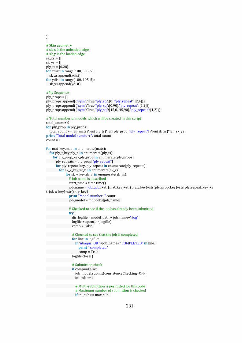
231

) # Skin geometry # sk_x is the unloaded edge # sk_y is the loaded edge sk_xs = [] sk_ys = [] ply_ts = [0.28] for xdist in range(100, 505, 5): sk_xs.append(xdist) for ydist in range(100, 105, 5): sk_ys.append(ydist) #Ply Sequence ply_props = [] ply_props.append({"sym":True,"ply_sq":[0],"ply_repeat":[2,4]}) ply_props.append({"sym":True,"ply_sq":[0,90],"ply_repeat":[1,2]}) ply_props.append({"sym":True,"ply_sq":[45,0,-45,90],"ply_repeat":[1,2]}) # Total number of models which will be created in this script total_count = 0 for ply_prop in ply_props: total_count += len(mats)*len(ply_ts)*len(ply_prop["ply_repeat"])*len(sk_xs)*len(sk_ys) print "Total model number: ", total_count count = 1 for mat_key,mat in enumerate(mats): for ply_t_key,ply_t in enumerate(ply_ts): for ply_prop_key,ply_prop in enumerate(ply_props): ply_repeats = ply_prop["ply_repeat"] for ply_repeat_key, ply_repeat in enumerate(ply_repeats): for sk_x_key,sk_x in enumerate(sk_xs): for sk_y_key,sk_y in enumerate(sk_ys): # Job name is described start_time = time.time() job_name ='job_cpb_'+str(mat_key)+str(ply_t_key)+str(ply_prop_key)+str(ply_repeat_key)+str(sk_x_key)+str(sk_y_key) print "Model number: ",count job_model = mdb.jobs[job_name] # Checked to see if the job has already been submitted try: dir_logfile = model_path + job_name+".log" logfile = open(dir_logfile) comp = False # Checked to see that the job is completed for line in logfile: if "Abaqus JOB "+job_name+" COMPLETED" in line: print " completed" comp = True logfile.close() # Submittion check if comp==False: job_model.submit(consistencyChecking=OFF) ini_sub +=1 # Multi-submittion is permitted for this code # Maximum number of submittion is checked if ini_sub >= max_sub:

232

job_model.waitForCompletion() ini_sub = 0 end_time = time.time() else: end_time = time.time() except: # Submit the job job_model.submit(consistencyChecking=OFF) ini_sub +=1 # Multi-submittion is permitted for this code # Maximum number of submittion is checked if ini_sub >= max_sub: job_model.waitForCompletion() ini_sub = 0 end_time = time.time() # Estimated time is calculated if count%(max_sub*2) == 0: em=divmod((total_count-count)*(end_time-start_time)/max_sub,60) en=divmod(em[0],60) print "Estimated remaning time: " ,en[0],en[1],em[1] count+=1 # Checked whether all analyses are completed for mat_key,mat in enumerate(mats): for ply_t_key,ply_t in enumerate(ply_ts): for ply_prop_key,ply_prop in enumerate(ply_props): ply_repeats = ply_prop["ply_repeat"] for ply_repeat_key, ply_repeat in enumerate(ply_repeats): for sk_x_key,sk_x in enumerate(sk_xs): for sk_y_key,sk_y in enumerate(sk_ys): job_name ='job_cpb_'+str(mat_key)+str(ply_t_key)+str(ply_prop_key)+str(ply_repeat_key)+str(sk_x_key)+str(sk_y_key) job_model.waitForCompletion() for mat_key,mat in enumerate(mats): for ply_t_key,ply_t in enumerate(ply_ts): for ply_prop_key,ply_prop in enumerate(ply_props): ply_repeats = ply_prop["ply_repeat"] for ply_repeat_key, ply_repeat in enumerate(ply_repeats): # Writing the input data into the result file results = open(result_path+"_"+str(mat_key)+str(ply_t_key)+str(ply_prop_key)+str(ply_repeat_key)+".txt","w+") results_excel = open(result_excel_path+"_"+str(mat_key)+str(ply_t_key)+str(ply_prop_key)+str(ply_repeat_key)+".txt","w+") # Writing the excel graphs' headings into the result file which is used to construct excel results_excel.write("%20s %20s %20s %20s %20s %20s" %("a0/b0","k0-2D*(E)","k0-2D*(C)","k0-2D*(F)","error(E-C)","error(E-F)" )+"\n"+"\n") # Writing the material properties into the result file results.write("%-25s %20s " %("Material description: ", mat["mat_des"])+"\n") results.write("%-25s %6.2f %-20s %6.2f %-20s %6.2f" %("Material E1: ", mat["E1"], " Material E2: ", mat["E2"], " Material Nu12: ", mat["Nu12"])+"\n") results.write("%-25s %6.2f %-20s %6.2f %-20s %6.2f" %("Material G12: ", mat["G12"], " Material G13: ", mat["G13"], " Material G23: ", mat["G23"])+"\n") # Writing the ply thickness and symmetric condition into the result file

233

results.write("%-25s %6.2f %-20s %10s" %("Ply thickness: ", ply_t," Ply symmetric: ", ply_prop["sym"])+"\n") # Ply directions and angles are described to use in A,B,D matrices ply_sq = [] for rep in range(ply_repeat): for ply_ang in ply_prop["ply_sq"]: ply_sq.append(ply_ang) if ply_prop["sym"]: for ply_ang in reversed(ply_sq): ply_sq.append(ply_ang) # Writing the ply directions and angles into the result file results.write("%-25s" %("Ply Directions: ")) for ply_ang in ply_sq: results.write("%6d" %(ply_ang)) results.write("\n"+"\n") for sk_x_key,sk_x in enumerate(sk_xs): for sk_y_key,sk_y in enumerate(sk_ys): # Defining the job name job_name ='job_cpb_'+str(mat_key)+str(ply_t_key)+str(ply_prop_key)+str(ply_repeat_key)+str(sk_x_key)+str(sk_y_key) # Obtain the eigenvalue (Critical buckling load according to FEA) dir_datfile = model_path + job_name+'.dat' wordlist = [] starttorecord = False datfile = open(dir_datfile) for line in datfile: if " MODE NO EIGENVALUE" in line: starttorecord = True for word in line.split(): if word=='THE': starttorecord = False if starttorecord: wordlist.append(word) if float(wordlist[4])>0.0: eigenvalue = float(wordlist[4]) elif float(wordlist[6])>0.0: eigenvalue = float(wordlist[6]) elif float(wordlist[8])>0.0: eigenvalue = float(wordlist[8]) else: eigenvalue = 0.0 datfile.close() # Total number of composite layers are calculated ply_n_total = len(ply_sq) h_tot = ply_n_total * ply_t # Each layers of "h" matrix is the vertical distance from the mid-plane of the plate (z=0) to the upper surface of the considered lamina(layer) h = [] for ply_n in range(ply_n_total+1): h.append(-h_tot/2.0 + ply_n * ply_t) # Initialize the A and D matrices D11=0.0; D12=0.0; D22=0.0; D66=0.0; A44=0.0; A55=0.0 #"kk" is the shear correction coefficient

234

kk = 5.0/6.0 # A and D matrices are calculated in this part for ply_n,ply_ang in enumerate(ply_sq): # In-plane compliance coefficients for orthotropic materials in material axis S11 = 1.0/mat["E1"] S12 = -mat["Nu12"]/mat["E1"] S22 = 1.0/mat["E2"] S66 = 1.0/mat["G12"] # In-plane elastic coefficients for orthotropic materials in material axis Q11 = S22/(S11*S22-S12**2.0) Q12 = -S12/(S11*S22-S12**2.0) Q22 = S11/(S11*S22-S12**2.0) Q66 = 1.0/S66 # Problem axis angle cosine and sine values cs = math.cos(ply_ang*math.pi/180.0) sn = math.sin(ply_ang*math.pi/180.0) # Transformation of in-plane elastic coefficients for orthotropic materials in problem axis bQ11 = Q11*cs**4+2.0*(Q12+2.0*Q66)*(cs**2.0)*(sn**2.0)+Q22*sn**4.0 bQ22 = Q11*sn**4+2.0*(Q12+2.0*Q66)*(cs**2.0)*(sn**2.0)+Q22*cs**4.0 bQ12 = Q12*cs**4+(Q11+Q22-4.0*Q66)*(cs**2.0)*(sn**2.0)+Q12*sn**4.0 bQ66 = (Q11+Q22-2.0*Q12)*(cs**2.0)*(sn**2.0)+Q66*((cs**2.0)-(sn**2.0))**2.0 #Q1=[G23 0 ; 0 G13] #T1 = [cs -sn; sn cs] #T1_inv = [cs sn; -sn cs] #bbQ = T1_inv * Q1 *T1 #bbQ is the 2x2 matrix bbQ44 = cs**2.0*mat["G23"]+sn**2.0*mat["G13"] bbQ55 = sn**2.0*mat["G23"]+cs**2.0*mat["G13"] # Necessary values of A and D matrices D11 += bQ11 * (h[ply_n+1]**3.0-h[ply_n]**3.0) D22 += bQ22 * (h[ply_n+1]**3.0-h[ply_n]**3.0) D12 += bQ12 * (h[ply_n+1]**3.0-h[ply_n]**3.0) D66 += bQ66 * (h[ply_n+1]**3.0-h[ply_n]**3.0) A44 += bbQ44 * (h[ply_n+1]-h[ply_n]) A55 += bbQ55 * (h[ply_n+1]-h[ply_n]) # D matrix values D11/=3.0 D22/=3.0 D12/=3.0 D66/=3.0 # Composite buckling parameters according to FEA D_star = (D12+2.0*D66)/(D11*D22)**0.5 ratio_a0b0 = (sk_x*(D22)**0.25)/(sk_y*(D11)**0.25) # Composite plate buckling coefficient according to FEA k0_E = (eigenvalue * sk_y**2.0)/(pi*(D11*D22)**0.5) k_E = k0_E-2.0*D_star # The Classical Laminated Plate Theory # Critical bucling load when n=1 and m variying # "a" equals to "sk_x" (unloaded edge) and "b" equals to "sk_y" (loaded edge) N_Cs = [] nn_Cs =[]

235

mm_Cs =[] pi = math.pi # Critical bucling load calculation for simply supported plate for num1 in range(1): nn_C = num1 + 1 for num2 in range(10): mm_C = num2 + 1 N_C = D11*(mm_C*pi/sk_x)**2.0+(2.0*D12+4.0*D66)*(pi/sk_y)**2.0+D22*(sk_x*pi/mm_C)**2.0*(1.0/sk_y)**4.0 nn_Cs.append(nn_C) mm_Cs.append(mm_C) N_Cs.append(N_C) N_key_C = N_Cs.index(min(N_Cs)) mm_cri_C = mm_Cs[N_key_C] nn_cri_C = nn_Cs[N_key_C] # Critical buckling load according to CLPT N_cri_C = N_Cs[N_key_C] # Percentage error of critical buckling load between FEA result and CLPT result N_err_C = abs(N_cri_C-eigenvalue)/eigenvalue*100.0 # Composite plate buckling coefficient according to CLPT k0_C = (N_cri_C * sk_y**2.0)/(pi*(D11*D22)**0.5) k_C = k0_C-2.0*D_star #The First-Order Shear Deformation Theory N_Fs = [] nn_Fs=[] mm_Fs =[] # Critical bucling load calculation for simply supported plate for num1 in range(10): nn_F = num1 + 1 for num2 in range(10): mm_F = num2 + 1 alpha = mm_F*pi/sk_x beta = nn_F*pi/sk_y C1 = -D11*alpha**2.0-D66*beta**2.0-A55*kk C2 = -D12*alpha*beta-D66*alpha*beta C3 = -A55*kk*alpha C4 = -D22*beta**2.0-D66*alpha**2.0-A44*kk C5 = -A44*kk*beta N_F = (C1*C5**2.0+alpha*C3*C2**2.0+beta*C2**2.0*C5+C3**2.0*C4-alpha*C1*C3*C4-beta*C1*C4*C5-2.0*C2*C3*C5)/(alpha**2.0*(C1*C4-C2**2.0)) mm_Fs.append(mm_F) nn_Fs.append(nn_F) N_Fs.append(N_F) N_key_F = N_Fs.index(min(N_Fs)) mm_cri_F = mm_Fs[N_key_F] nn_cri_F = nn_Fs[N_key_F] # Critical buckling load according to FSDT N_cri_F = N_Fs[N_key_F] # Percentage error of critical buckling load between FEA result and FSDT result N_err_F = abs(N_cri_F-eigenvalue)/eigenvalue*100.0 # Composite plate buckling coefficient according to FSDT k0_F = (N_cri_F * sk_y**2.0)/(pi*(D11*D22)**0.5)

236

k_F = k0_F-2.0*D_star # Write the output data into the result file results.write("%-25s %6.2f %-20s %6.2f %-20s %6.2f" %(" Skin length y: ", sk_y, " Skin length x: ", sk_x, " Total thickness: ",h_tot )+"\n") results.write("%-25s %6.2f %-20s %6.2f %-20s %6.2f %-20s %6.2f %-20s %6.2f" %(" Eigenvalue: ",eigenvalue, " CLPT N (m="+str(mm_cri_C)+" and n="+str(nn_cri_C)+"): ", N_cri_C, " FSDT N (m="+str(mm_cri_F)+" and n="+str(nn_cri_F)+"): ",N_cri_F, " CLPT error %: ",N_err_C, " FSDT error %: ",N_err_F)+"\n"+"\n") # Write the output data into the result excel file results_excel.write("%20.2f %20.2f %20.2f %20.2f %20.2f %20.2f" %(ratio_a0b0, k_E, k_C, k_F, N_err_C, N_err_F )+"\n") results.close() results_excel.close() # Saving the model mdb.saveAs(pathName=save_path+'.cae') # Stoping the time calculater end_t_time = time.time() m=divmod(end_t_time-start_t_time,60) n=divmod(m[0],60) print "Total time: " ,n[0],n[1],m[1]

• Example code to construct the composite panel model with clamped boundary

condition

# Importing necessary modules from abaqus import * from abaqusConstants import * from caeModules import * from driverUtils import executeOnCaeStartup from part import * from material import * from section import * from assembly import * from step import * from interaction import * from load import * from mesh import * from optimization import * from job import * from sketch import * from visualization import * from connectorBehavior import * import math import time # Counter for script time start_t_time = time.time() # Paths

237

save_path='C:/Users/……………………………………./Model/cl/comp_cl_buckling' # Given edge load (N/mm) Edge_load = 1.0 # Material properties # In this case, material is Carbon/epoxy,Hexply 8552S/37RC/AGP280/C mats=[] mats.append( { "mat_des" : "Carbon_epoxy", "E1":54000, "E2":54000, "Nu12":0.05, "G12":4.5e3, "G13":4.5e3, "G23":4.5e3} ) # Skin geometry # sk_x is the unloaded edge # sk_y is the loaded edge sk_xs = [] sk_ys = [] ply_ts = [0.28] for xdist in range(100, 505, 5): sk_xs.append(xdist) for ydist in range(100, 105, 5): sk_ys.append(ydist) #Ply sequences ply_props = [] ply_props.append({"sym":True,"ply_sq":[0],"ply_repeat":[2,4]}) ply_props.append({"sym":True,"ply_sq":[0,90],"ply_repeat":[1,2]}) ply_props.append({"sym":True,"ply_sq":[45,0,-45,90],"ply_repeat":[1,2]}) # Total number of models which will be created in this script total_count = 0 for ply_prop in ply_props: total_count += len(mats)*len(ply_ts)*len(ply_prop["ply_repeat"])*len(sk_xs)*len(sk_ys) print "Total model number: ", total_count for mat_key,mat in enumerate(mats): for ply_t_key,ply_t in enumerate(ply_ts): for ply_prop_key,ply_prop in enumerate(ply_props): ply_repeats = ply_prop["ply_repeat"] for ply_repeat_key, ply_repeat in enumerate(ply_repeats): for sk_x_key,sk_x in enumerate(sk_xs): for sk_y_key,sk_y in enumerate(sk_ys): # Creating model of composite panel buckling (cpb) print "Creating model" model_name = "cpb_"+str(mat_key)+str(ply_t_key)+str(ply_prop_key)+str(ply_repeat_key)+str(sk_x_key)+str(sk_y_key) mdb.Model(modelType=STANDARD_EXPLICIT, name=model_name) mn=mdb.models[model_name] # Creating material print "Creating model" mn.Material(name=mat["mat_des"]) mn.materials[mat["mat_des"]].Elastic( type=LAMINA, table=(( mat["E1"], mat["E2"],mat["Nu12"], mat["G12"], mat["G13"], mat["G23"]), )) # Creating sketch of skin print "Creating sketch of skin"

238

mn.ConstrainedSketch(name='__profile__', sheetSize=200.0) mn.sketches['__profile__'].rectangle(point1=(0.0, 0.0), point2=(sk_x, sk_y)) # Creating part of skin print "Creating part of skin" mn.Part(dimensionality=THREE_D, name='Skin', type=DEFORMABLE_BODY) mn.parts['Skin'].BaseShell(sketch=mn.sketches['__profile__']) del mn.sketches['__profile__'] # Creating Layup orientation print "Creating Layup orientation" layupOrientation = None p_sk = mn.parts['Skin'] f_sk, e_sk, d_sk = p_sk.faces, p_sk.edges, p_sk.datums faces = f_sk.getSequenceFromMask(mask=('[#1 ]', ), ) region_sk=regionToolset.Region(faces=faces) compositeLayup = p_sk.CompositeLayup( name='CompositeLayup-1', description='', elementType=SHELL, offsetType=MIDDLE_SURFACE, symmetric=ply_prop["sym"], thicknessAssignment=FROM_SECTION) compositeLayup.Section(preIntegrate=OFF, integrationRule=SIMPSON, thicknessType=UNIFORM, poissonDefinition=DEFAULT, temperature=GRADIENT, useDensity=OFF) compositeLayup.ReferenceOrientation(orientationType=GLOBAL, localCsys=None, fieldName='', additionalRotationType=ROTATION_NONE, angle=0.0, axis=AXIS_3) ply_sq = [] for rep in range(ply_repeat): for ply_ang in ply_prop["ply_sq"]: ply_sq.append(ply_ang) for ply_n,ply_ang in enumerate(ply_sq): compositeLayup.CompositePly(suppressed=False, plyName='Ply-'+str(ply_n+1), region=region_sk, material=mat["mat_des"], thicknessType=SPECIFY_THICKNESS, thickness=ply_t, orientationType=SPECIFY_ORIENT, orientationValue=ply_ang, additionalRotationType=ROTATION_NONE, additionalRotationField='', axis=AXIS_3, angle=0.0, numIntPoints=3) # Mesh control of skin print "Mesh control of skin" pickedRegions = f_sk.getSequenceFromMask(mask=('[#1 ]', ), ) p_sk.setMeshControls(regions=pickedRegions, elemShape=QUAD, technique=SWEEP) # Mesh seed of skin print "Mesh seed of skin" p_sk.seedPart(deviationFactor=0.1, minSizeFactor=0.1, size=5.0) # Generate mesh of skin print "Generate mesh of skin" p_sk.generateMesh() # Creating buckling step print "Creating Buckling step" mn.BuckleStep(name='Buckle-Step', previous='Initial', numEigen=8, vectors=28, maxIterations=3000) # Creating assembly instances print "Creating assembly instances" a_sk = mn.rootAssembly a_sk.DatumCsysByDefault(CARTESIAN) a_sk.Instance(dependent=ON, name='Skin-1', part=p_sk) # Creating boundary conditions at initial step

239

print "Creating boundary conditions at initial step" edges_bc = {'[#2 ]':'loaded_edge','[#8 ]':'opp_loaded_edge','[#5 ]':'unloaded_edges'} e_sk = a_sk.instances['Skin-1'].edges for edge_key,edge_des in edges_bc.items(): edges1 = e_sk.getSequenceFromMask(mask=(edge_key, ), ) a_sk.Set(edges=edges1, name='Set_'+edge_des) v_sk = a_sk.instances['Skin-1'].vertices verts_bc = {'[#8 ]':'lb_cor','[#2 ]':'rt_cor'} for vert_key,vert_des in verts_bc.items(): verts1 = v_sk.getSequenceFromMask(mask=(vert_key, ), ) a_sk.Set(vertices=verts1, name='Set_'+vert_des) # Assigning boundary conditions using sets print "Assigning boundary conditions using sets" region = a_sk.sets['Set_lb_cor'] mn.DisplacementBC(name='BC_lb_cor', createStepName='Initial', region=region, u1=SET, u2=SET, u3=SET, ur1=UNSET, ur2=UNSET, ur3=UNSET, amplitude=UNSET, distributionType=UNIFORM, fieldName='', localCsys=None) region = a_sk.sets['Set_rt_cor'] mn.DisplacementBC(name='BC_rt_cor', createStepName='Initial', region=region, u1=UNSET, u2=SET, u3=UNSET, ur1=UNSET, ur2=UNSET, ur3=UNSET, amplitude=UNSET, distributionType=UNIFORM, fieldName='', localCsys=None) region = a_sk.sets['Set_loaded_edge'] mn.DisplacementBC(name='BC_loaded_edge', createStepName='Initial', region=region, u1=UNSET, u2=UNSET, u3=SET, ur1=UNSET, ur2=SET, ur3=UNSET, amplitude=UNSET, distributionType=UNIFORM, fieldName='', localCsys=None) region = a_sk.sets['Set_opp_loaded_edge'] mn.DisplacementBC(name='BC_opp_loaded_edge', createStepName='Initial', region=region, u1=SET, u2=UNSET, u3=SET, ur1=UNSET, ur2=SET, ur3=UNSET, amplitude=UNSET, distributionType=UNIFORM, fieldName='', localCsys=None) region = a_sk.sets['Set_unloaded_edges'] mn.DisplacementBC(name='BC_unloaded_edges', createStepName='Initial', region=region, u1=UNSET, u2=UNSET, u3=SET, ur1=SET, ur2=UNSET, ur3=UNSET, amplitude=UNSET, distributionType=UNIFORM, fieldName='', localCsys=None) # Appliying shell edge load on the skin loaded edge print "Appliying shell edge load on the skin loaded edge" load_edges=['[#2 ]'] for load_key,load_edge in enumerate(load_edges): s_edges = e_sk.getSequenceFromMask(mask=(load_edge, ), ) region = a_sk.Surface(side1Edges=s_edges, name='Surf_loaded_edge'+str(load_key+1)) mn.ShellEdgeLoad(name='Load_buckling'+str(load_key+1), createStepName='Buckle-Step', region=region, magnitude=Edge_load, distributionType=UNIFORM, field='', localCsys=None) # Creating job print "Creating job" job_name ='job_'+ model_name mdb.Job(name=job_name, model=model_name, description='', type=ANALYSIS, atTime=None, waitMinutes=0, waitHours=0, queue=None, memory=90, memoryUnits=PERCENTAGE, getMemoryFromAnalysis=True, explicitPrecision=SINGLE, nodalOutputPrecision=SINGLE, echoPrint=OFF, modelPrint=OFF, contactPrint=OFF, historyPrint=OFF, userSubroutine='', scratch='', resultsFormat=ODB, multiprocessingMode=DEFAULT, numCpus=1, numGPUs=0) try: del mdb.models['Model-1'] except: None

240

# Saving the model print "Saving model" mdb.saveAs(pathName=save_path+'.cae') # Stoping the time calculater end_t_time = time.time() m=divmod(end_t_time-start_t_time,60) n=divmod(m[0],60) print "Total time: " ,n[0],n[1],m[1]

• Example code to process finite element results for the composite panel model with

clamped boundary condition

# Importing necessary modules from abaqus import * from abaqusConstants import * from caeModules import * from driverUtils import executeOnCaeStartup from part import * from material import * from section import * from assembly import * from step import * from interaction import * from load import * from mesh import * from optimization import * from job import * from sketch import * from visualization import * from connectorBehavior import * import math import time # Counter for script time start_t_time = time.time() # Defining maximum number of submittions can be given at the same time max_sub = 5 ini_sub = 0 # Paths save_path='C:/Users/……………………………………./Model/cl/comp_cl_buckling' model_path = r'C:/Users/……………………………………./Model/cl/' # Initialize results' path result_path = r"C:\Users\…………………………………….\Results\comp_cl_buckling_loads" result_excel_path = r"C:\Users\…………………………………….\Results\excel\comp_cl_buckling_loads" # Given edge load (N/mm) Edge_load = 1.0 # Material properties # In this case, material is Carbon/epoxy,Hexply 8552S/37RC/AGP280/C mats=[] mats.append( { "mat_des" : "Carbon_epoxy", "E1":54000, "E2":54000, "Nu12":0.05, "G12":4.5e3, "G13":4.5e3, "G23":4.5e3}

241

) # Skin geometry # sk_x is the unloaded edge # sk_y is the loaded edge sk_xs = [] sk_ys = [] ply_ts = [0.28] for xdist in range(100, 505, 5): sk_xs.append(xdist) for ydist in range(100, 105, 5): sk_ys.append(ydist) #Ply Sequence ply_props = [] ply_props.append({"sym":True,"ply_sq":[0],"ply_repeat":[2,4]}) ply_props.append({"sym":True,"ply_sq":[0,90],"ply_repeat":[1,2]}) ply_props.append({"sym":True,"ply_sq":[45,0,-45,90],"ply_repeat":[1,2]}) # Total number of models which will be created in this script total_count = 0 for ply_prop in ply_props: total_count += len(mats)*len(ply_ts)*len(ply_prop["ply_repeat"])*len(sk_xs)*len(sk_ys) print "Total model number: ", total_count count = 1 for mat_key,mat in enumerate(mats): for ply_t_key,ply_t in enumerate(ply_ts): for ply_prop_key,ply_prop in enumerate(ply_props): ply_repeats = ply_prop["ply_repeat"] for ply_repeat_key, ply_repeat in enumerate(ply_repeats): for sk_x_key,sk_x in enumerate(sk_xs): for sk_y_key,sk_y in enumerate(sk_ys): # Job name is described start_time = time.time() job_name ='job_cpb_'+str(mat_key)+str(ply_t_key)+str(ply_prop_key)+str(ply_repeat_key)+str(sk_x_key)+str(sk_y_key) print "Model number: ",count job_model = mdb.jobs[job_name] # Checked to see if the job has already been submitted try: dir_logfile = model_path + job_name+".log" logfile = open(dir_logfile) comp = False # Checked to see that the job is completed for line in logfile: if "Abaqus JOB "+job_name+" COMPLETED" in line: print " completed" comp = True logfile.close() # Submittion check if comp==False: job_model.submit(consistencyChecking=OFF) ini_sub +=1 # Multi-submittion is permitted for this code # Maximum number of submittion is checked if ini_sub >= max_sub:

242

job_model.waitForCompletion() ini_sub = 0 end_time = time.time() else: end_time = time.time() except: # Submit the job job_model.submit(consistencyChecking=OFF) ini_sub +=1 # Multi-submittion is permitted for this code # Maximum number of submittion is checked if ini_sub >= max_sub: job_model.waitForCompletion() ini_sub = 0 end_time = time.time() # Estimated time is calculated if count%(max_sub*2) == 0: em=divmod((total_count-count)*(end_time-start_time)/max_sub,60) en=divmod(em[0],60) print "Estimated remaning time: " ,en[0],en[1],em[1] count+=1 # Checked whether all analyses are completed for mat_key,mat in enumerate(mats): for ply_t_key,ply_t in enumerate(ply_ts): for ply_prop_key,ply_prop in enumerate(ply_props): ply_repeats = ply_prop["ply_repeat"] for ply_repeat_key, ply_repeat in enumerate(ply_repeats): for sk_x_key,sk_x in enumerate(sk_xs): for sk_y_key,sk_y in enumerate(sk_ys): job_name ='job_cpb_'+str(mat_key)+str(ply_t_key)+str(ply_prop_key)+str(ply_repeat_key)+str(sk_x_key)+str(sk_y_key) job_model.waitForCompletion() for mat_key,mat in enumerate(mats): for ply_t_key,ply_t in enumerate(ply_ts): for ply_prop_key,ply_prop in enumerate(ply_props): ply_repeats = ply_prop["ply_repeat"] for ply_repeat_key, ply_repeat in enumerate(ply_repeats): # Writing the input data into the result file results = open(result_path+"_"+str(mat_key)+str(ply_t_key)+str(ply_prop_key)+str(ply_repeat_key)+".txt","w+") results_excel = open(result_excel_path+"_"+str(mat_key)+str(ply_t_key)+str(ply_prop_key)+str(ply_repeat_key)+".txt","w+") # Writing the excel graphs' headings into the result file which is used to construct excel results_excel.write("%20s %20s %20s %20s %20s %20s" %("a0/b0","k0-2D*(E)","k0-2D*(C)","k0-2D*(F)","error(E-C)","error(E-F)" )+"\n"+"\n") # Writing the material properties into the result file results.write("%-25s %20s " %("Material description: ", mat["mat_des"])+"\n") results.write("%-25s %6.2f %-20s %6.2f %-20s %6.2f" %("Material E1: ", mat["E1"], " Material E2: ", mat["E2"], " Material Nu12: ", mat["Nu12"])+"\n") results.write("%-25s %6.2f %-20s %6.2f %-20s %6.2f" %("Material G12: ", mat["G12"], " Material G13: ", mat["G13"], " Material G23: ", mat["G23"])+"\n")

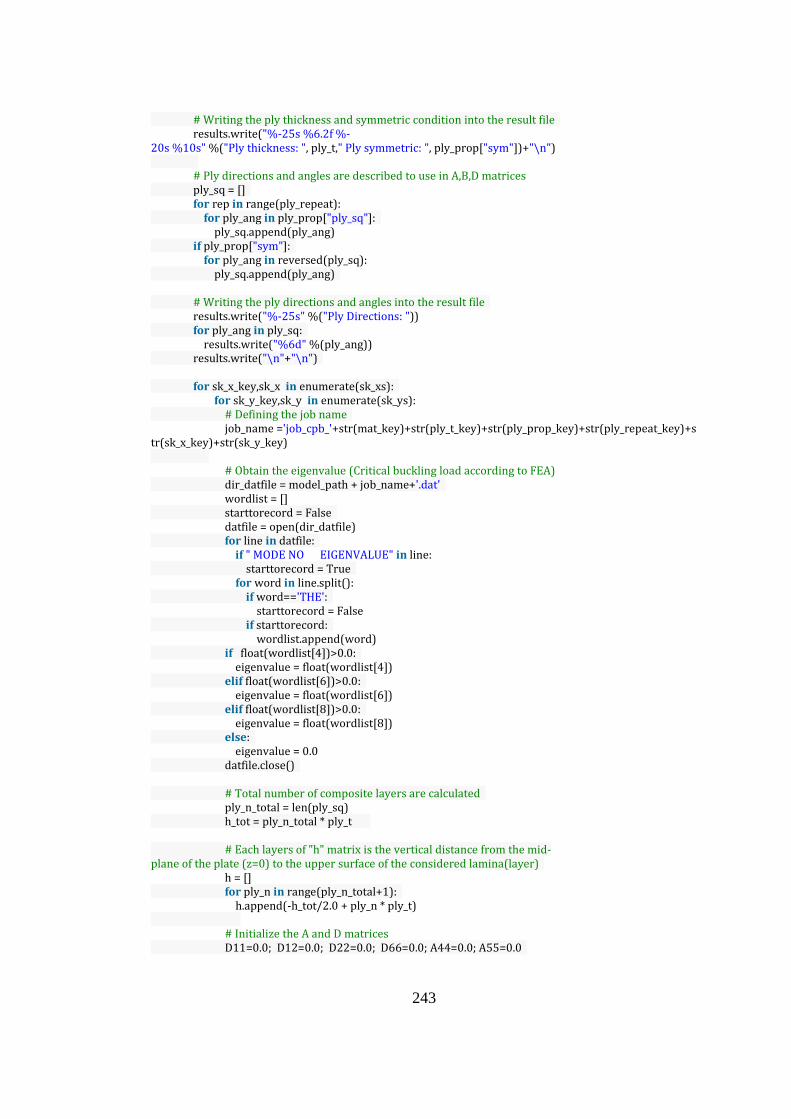
243

# Writing the ply thickness and symmetric condition into the result file results.write("%-25s %6.2f %-20s %10s" %("Ply thickness: ", ply_t," Ply symmetric: ", ply_prop["sym"])+"\n") # Ply directions and angles are described to use in A,B,D matrices ply_sq = [] for rep in range(ply_repeat): for ply_ang in ply_prop["ply_sq"]: ply_sq.append(ply_ang) if ply_prop["sym"]: for ply_ang in reversed(ply_sq): ply_sq.append(ply_ang) # Writing the ply directions and angles into the result file results.write("%-25s" %("Ply Directions: ")) for ply_ang in ply_sq: results.write("%6d" %(ply_ang)) results.write("\n"+"\n") for sk_x_key,sk_x in enumerate(sk_xs): for sk_y_key,sk_y in enumerate(sk_ys): # Defining the job name job_name ='job_cpb_'+str(mat_key)+str(ply_t_key)+str(ply_prop_key)+str(ply_repeat_key)+str(sk_x_key)+str(sk_y_key) # Obtain the eigenvalue (Critical buckling load according to FEA) dir_datfile = model_path + job_name+'.dat' wordlist = [] starttorecord = False datfile = open(dir_datfile) for line in datfile: if " MODE NO EIGENVALUE" in line: starttorecord = True for word in line.split(): if word=='THE': starttorecord = False if starttorecord: wordlist.append(word) if float(wordlist[4])>0.0: eigenvalue = float(wordlist[4]) elif float(wordlist[6])>0.0: eigenvalue = float(wordlist[6]) elif float(wordlist[8])>0.0: eigenvalue = float(wordlist[8]) else: eigenvalue = 0.0 datfile.close() # Total number of composite layers are calculated ply_n_total = len(ply_sq) h_tot = ply_n_total * ply_t # Each layers of "h" matrix is the vertical distance from the mid-plane of the plate (z=0) to the upper surface of the considered lamina(layer) h = [] for ply_n in range(ply_n_total+1): h.append(-h_tot/2.0 + ply_n * ply_t) # Initialize the A and D matrices D11=0.0; D12=0.0; D22=0.0; D66=0.0; A44=0.0; A55=0.0

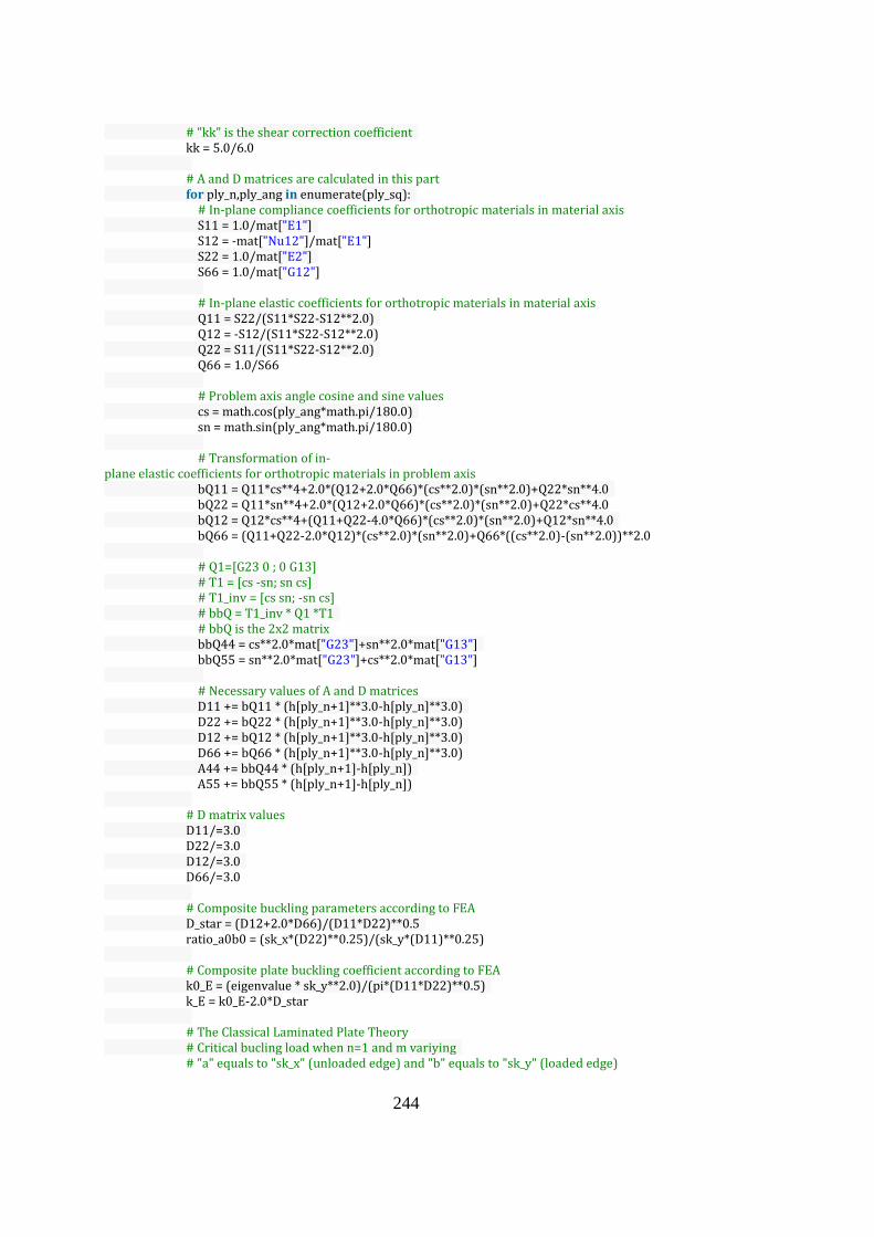
244

# "kk" is the shear correction coefficient kk = 5.0/6.0 # A and D matrices are calculated in this part for ply_n,ply_ang in enumerate(ply_sq): # In-plane compliance coefficients for orthotropic materials in material axis S11 = 1.0/mat["E1"] S12 = -mat["Nu12"]/mat["E1"] S22 = 1.0/mat["E2"] S66 = 1.0/mat["G12"] # In-plane elastic coefficients for orthotropic materials in material axis Q11 = S22/(S11*S22-S12**2.0) Q12 = -S12/(S11*S22-S12**2.0) Q22 = S11/(S11*S22-S12**2.0) Q66 = 1.0/S66 # Problem axis angle cosine and sine values cs = math.cos(ply_ang*math.pi/180.0) sn = math.sin(ply_ang*math.pi/180.0) # Transformation of in-plane elastic coefficients for orthotropic materials in problem axis bQ11 = Q11*cs**4+2.0*(Q12+2.0*Q66)*(cs**2.0)*(sn**2.0)+Q22*sn**4.0 bQ22 = Q11*sn**4+2.0*(Q12+2.0*Q66)*(cs**2.0)*(sn**2.0)+Q22*cs**4.0 bQ12 = Q12*cs**4+(Q11+Q22-4.0*Q66)*(cs**2.0)*(sn**2.0)+Q12*sn**4.0 bQ66 = (Q11+Q22-2.0*Q12)*(cs**2.0)*(sn**2.0)+Q66*((cs**2.0)-(sn**2.0))**2.0 # Q1=[G23 0 ; 0 G13] # T1 = [cs -sn; sn cs] # T1_inv = [cs sn; -sn cs] # bbQ = T1_inv * Q1 *T1 # bbQ is the 2x2 matrix bbQ44 = cs**2.0*mat["G23"]+sn**2.0*mat["G13"] bbQ55 = sn**2.0*mat["G23"]+cs**2.0*mat["G13"] # Necessary values of A and D matrices D11 += bQ11 * (h[ply_n+1]**3.0-h[ply_n]**3.0) D22 += bQ22 * (h[ply_n+1]**3.0-h[ply_n]**3.0) D12 += bQ12 * (h[ply_n+1]**3.0-h[ply_n]**3.0) D66 += bQ66 * (h[ply_n+1]**3.0-h[ply_n]**3.0) A44 += bbQ44 * (h[ply_n+1]-h[ply_n]) A55 += bbQ55 * (h[ply_n+1]-h[ply_n]) # D matrix values D11/=3.0 D22/=3.0 D12/=3.0 D66/=3.0 # Composite buckling parameters according to FEA D_star = (D12+2.0*D66)/(D11*D22)**0.5 ratio_a0b0 = (sk_x*(D22)**0.25)/(sk_y*(D11)**0.25) # Composite plate buckling coefficient according to FEA k0_E = (eigenvalue * sk_y**2.0)/(pi*(D11*D22)**0.5) k_E = k0_E-2.0*D_star # The Classical Laminated Plate Theory # Critical bucling load when n=1 and m variying # "a" equals to "sk_x" (unloaded edge) and "b" equals to "sk_y" (loaded edge)

245

N_Cs = [] nn_Cs =[] mm_Cs =[] pi = math.pi # Critical bucling load calculation for clamped plate for num1 in range(10): nn_C = num1 + 1 for num2 in range(10): mm_C = num2 + 1 if nn_C==mm_C: N_C = (4.0*pi**2.0*D11*mm_C**2.0)/sk_x**2.0+(4.0*pi**2.0*D22*sk_x**2.0)/(sk_y**4.0*mm_C**2.0)+16.0*pi**2.0/(3.0*sk_y**2.0)*(0.5*D12+D66) else: N_C = (D11*pi**2.0/sk_x**2.0*(nn_C**4.0+6.0*nn_C**2.0*mm_C**2.0+mm_C**4.0)+D22*pi**2.0*16.0*sk_x**2.0/(3.0*sk_y**4.0)+(0.5*D12+D66)*16.0*pi**2.0/(3.0*sk_y**2.0)*(nn_C**2.0+mm_C**2.0))/(nn_C**2.0+mm_C**2.0) nn_Cs.append(nn_C) mm_Cs.append(mm_C) N_Cs.append(N_C) N_key_C = N_Cs.index(min(N_Cs)) mm_cri_C = mm_Cs[N_key_C] nn_cri_C = nn_Cs[N_key_C] # Critical buckling load according to CLPT N_cri_C = N_Cs[N_key_C] # Percentage error of critical buckling load between FEA result and CLPT result N_err_C = abs(N_cri_C-eigenvalue)/eigenvalue*100.0 # Composite plate buckling coefficient according to CLPT k0_C = (N_cri_C * sk_y**2.0)/(pi*(D11*D22)**0.5) k_C = k0_C-2.0*D_star #The First-Order Shear Deformation Theory N_Fs = [] nn_Fs=[] mm_Fs =[] # Critical bucling load calculation for clamped plate for num1 in range(10): nn_F = num1 + 1 for num2 in range(10): mm_F = num2 + 1 if(1.0-2.0*nn_F**2.0+mm_F**4.0-2.0*mm_F**2.0*nn_F**2.0-2.0*mm_F**2.0+nn_F**4.0)!=0.0 : if mm_F==1: G1 = pi**4.0*(3.0*D11*sk_y**4.0+2.0*D12*sk_x**2.0*sk_y**2.0+3.0*D22*sk_x**4.0+4.0*D66*sk_x**2.0*sk_y**2.0)/(4.0*sk_x**3.0*sk_y**3.0) G2 = -(pi**2.0*sk_y*(3.0*nn_F**4.0-12.0*nn_F**2.0))/(16.0*sk_x*(nn_F**4.0-4.0*nn_F**2.0)) G3 = -(8.0*sk_y*(-nn_F**3.0+(-1.0)**(nn_F+2.0)*nn_F**3.0))/(3.0*sk_x*(nn_F**4.0-4.0*nn_F**2.0)) G4 = kk*pi**2.0*(A44*sk_x**2.0+A55*nn_F**2.0*sk_y**2.0)/(4.0*sk_x*sk_y) G5 = -(pi**2.0*sk_y*(nn_F**6.0-4.0*nn_F**4.0))/(4.0*sk_x*(nn_F**4.0-4.0*nn_F**2.0)) N_F = (-(G1*G5+G2*G4)-((G1*G5+G2*G4)**2.0-4.0*(G2*G5-G3**2.0)*G1*G4)**0.5)/(2.0*(G2*G5-G3**2.0)) else:

246

H1 = pi**4.0*(D11*sk_y**4.0*(18.0*mm_F**2.0+3.0+3.0*mm_F**4.0)+D12*sk_x**2.0*sk_y**2.0*(8.0+8.0*mm_F**2.0)+16.0*D22*sk_x**4.0+D66*sk_x**2.0*sk_y**2.0*(16.0+16.0*mm_F**2.0))/(32.0*sk_x**3.0*sk_y**3.0) H2 = -(pi**2.0*sk_y*(3.0*mm_F**6.0+3.0+3.0*nn_F**4.0-3.0*mm_F**4.0-3.0*mm_F**2.0+3.0*mm_F**2.0*nn_F**4.0-12.0*mm_F**2.0*nn_F**2.0-6.0*nn_F**2.0-6.0*mm_F**4.0*nn_F**2.0))/(32.0*sk_x*(1.0-2.0*nn_F**2.0+mm_F**4.0-2.0*mm_F**2.0*nn_F**2.0-2.0*mm_F**2.0+nn_F**4.0)) H3 = -(8.0*sk_y*(-mm_F*nn_F**3.0+(-1.0)**(mm_F+nn_F+1.0)*mm_F*nn_F**3.0))/(3.0*sk_x*(1.0-2.0*nn_F**2.0+mm_F**4.0-2.0*mm_F**2.0*nn_F**2.0-2.0*mm_F**2.0+nn_F**4.0)) H4 = kk*pi**2.0*(A44*sk_x**2.0+A55*nn_F**2.0*sk_y**2.0)/(4.0*sk_x*sk_y) H5 = -(pi**2.0*sk_y*(nn_F**2.0+nn_F**6.0-2.0*mm_F**2.0*nn_F**4.0+mm_F**4.0*nn_F**2.0-2.0*nn_F**4.0-2.0*mm_F**2.0*nn_F**2.0))/(4.0*sk_x*(1.0-2.0*nn_F**2.0+mm_F**4.0-2.0*mm_F**2.0*nn_F**2.0-2.0*mm_F**2.0+nn_F**4.0)) N_F = (-(H1*H5+H2*H4)-((H1*H5+H2*H4)**2.0-4.0*(H2*H5-H3**2.0)*H1*H4)**0.5)/(2.0*(H2*H5-H3**2.0)) mm_Fs.append(mm_F) nn_Fs.append(nn_F) N_Fs.append(N_F) N_key_F = N_Fs.index(min(N_Fs)) mm_cri_F = mm_Fs[N_key_F] nn_cri_F = nn_Fs[N_key_F] # Critical buckling load according to FSDT N_cri_F = N_Fs[N_key_F] # Percentage error of critical buckling load between FEA result and FSDT result N_err_F = abs(N_cri_F-eigenvalue)/eigenvalue*100.0 # Composite plate buckling coefficient according to FSDT k0_F = (N_cri_F * sk_y**2.0)/(pi*(D11*D22)**0.5) k_F = k0_F-2.0*D_star # Write the output data into the result file results.write("%-25s %6.2f %-20s %6.2f %-20s %6.2f" %(" Skin length y: ", sk_y, " Skin length x: ", sk_x, " Total thickness: ",h_tot )+"\n") results.write("%-25s %6.2f %-20s %6.2f %-20s %6.2f %-20s %6.2f %-20s %6.2f" %(" Eigenvalue: ",eigenvalue, " CLPT N (m="+str(mm_cri_C)+" and n="+str(nn_cri_C)+"): ", N_cri_C, " FSDT N (m="+str(mm_cri_F)+" and n="+str(nn_cri_F)+"): ",N_cri_F, " CLPT error %: ",N_err_C, " FSDT error %: ",N_err_F)+"\n"+"\n") # Write the output data into the result excel file results_excel.write("%20.2f %20.2f %20.2f %20.2f %20.2f %20.2f" %(ratio_a0b0, k_E, k_C, k_F, N_err_C, N_err_F )+"\n") results.close() results_excel.close() # Saving the model mdb.saveAs(pathName=save_path+'.cae') # Stoping the time calculater end_t_time = time.time() m=divmod(end_t_time-start_t_time,60) n=divmod(m[0],60) print "Total time: " ,n[0],n[1],m[1]

Documents

Post-Buckling Behaviour Of Metallic Skin-Stringer