Portfolio Choice and Trading Volume with Loss-Averse InvestorsFrancisco J. Gomes1

London Business School

March 2003

Abstract

This paper presents a model of portfolio choice and stock trading volume with loss-

averse investors. The demand function for risky assets is discontinuous and non-monotonic:

as wealth rises beyond a threshold investors follow a generalized portfolio insurance strategy.

This behavior is consistent with the evidence in favor of the disposition effect. In addition,

loss-averse investors will not hold stocks unless the equity premium is quite high. The

elasticity of the aggregate demand curve changes substantially, depending on the distribution

of wealth across investors. In an equilibrium setting the model generates positive correlation

between trading volume and stock return volatility, but suggests that this relationship should

be non-linear.

Key Words: Loss Aversion, First-Order Risk Aversion, Portfolio Insurance, Portfolio

Choice, Stock Market Participation, Trading Volume

JEL Classification: G11, G12

1This paper has benefited from the comments and suggestions made by Leandro Arozamena, Nicholas

Barberis, Estelle Cantillon, John Campbell, Laurent Calvet, João Cocco, Wayne Ferson, Benjamin Friedman,

João Gomes, David Laibson, Andrew Metrick, Sendhil Mullainathan, Andrei Shleifer, Raman Uppal, Haiying

Wang, an anonymous referee, and seminar participants at Boston College, C.E.M.F.I., Duke, Harvard, L.B.S.,

New University of Lisbon, M.I.T., University of Cyprus, U.S.C., Washington, Yale and at the EFA 2000.

Previous versions of this paper have circulated with the tittle "Loss Aversion and the Demand for Risky

Assets". Financial support from the Sloan Foundation is gratefully appreciated. The usual disclaimer

applies. Corresponding address: Francisco Gomes, London Business School, Regent’s Park, London, NW1

4SA; United Kingdom. E-mail: fgomes@london.edu.

1

1 Introduction

“Value should be treated as a function in two arguments: the asset position that serves as a

reference point, and the magnitude of the change (positive or negative) from that reference

point”, Kahneman and Tversky (1979).

This paper solves a model of portfolio choice and trading volume with loss-averse in-

vestors. Loss aversion specifies that individuals value wealth relative to a given reference

point, that they are (much) more sensitive to losses than to gains (both measured relative

to the reference point), and that they are risk-averse in the domain of gains and risk-loving

in the domain of (moderate) losses. The first property is summarized in the above quote

from Kahneman and Tversky (1979). The second property corresponds to the notion of first-

order risk aversion as discussed by Epstein and Zin (1990). It implies that agents exhibit

significant risk aversion even for very small gambles. The last property states that following

losses the investor is more willing to take additional risks (so as to be able to go back to the

break-even point), while following gains she will be more conservative.

If investors exhibit first-order risk aversion and their attitudes towards risk are a function

of the past performance of their investments, then this will have important implications for

the demand for risky assets and, in equilibrium, for the conditional distribution of stock

returns and for trading volume.

We start by studying the optimal portfolio allocation behavior of a loss-averse investor.

This behavior depends crucially on the level of surplus wealth (current wealth relative to the

reference point), and on how the investor’s reference point reacts to changes in the current

stock price. As surplus wealth reaches a certain threshold, the investor sells a significant part

of her stock holdings and follows a (generalized) portfolio insurance rule, protecting herself

against losses (relative to her reference point). Intuitively, as the stock price goes up, the

investor faces a trade-off between the potential benefit from insuring herself against losses and

the cost of doing so: selling a large share of her portfolio and giving up the equity premium.

As the stock price rises further, and surplus wealth keeps increasing, the cost of switch to the

portfolio insurance rule becomes smaller: the investor doesn’t have to sell as many stocks.

Therefore, as the price rises enough she eventually switches. This generates a behavior

2

consistent with the disposition effect: investors have a larger tendency to sell their winners

and to hold on to their losers (see Shefrin and Statman (1985) and Odean (1998), among

others). In addition, this provides a rational motivation for portfolio insurance strategies,

and identifies the conditions under which investors are more or less likely to follow these

strategies. Finally, loss-averse investors will abstain from holding equities unless they expect

the equity premium to be quite large, and therefore these preferences can help to explain

the low stock market participation rates observed in the data.

Heterogeneity in surplus wealth across investors generates trading volume, even in a per-

fect information setting. We consider a general equilibriummodel with two types of investors:

one type with power utility and another type exhibiting loss-aversion. This corresponds to

a symmetric information version of the model in He and Wang (1995), but with CRRA

and Loss-Averse investors instead of CARA investors. Alternatively, it also corresponds

to a discrete-time version of the models in Grossman and Zhou (1996) or Basak (1995),

but where the demand for portfolio insurance is endogenous and time varying. Basak (2002)

also develops a model in which the demand for portfolio insurance is endogenously generated

by the investor’s preferences. Our models differ because we consider a different preference

specification, and because he studies the implications for stock return volatility and for risk

premia, while we are concerned with trading volume and with characterizing the portfolio

rules specifically generated by the loss-aversion preferences.

The equilibrium model is solved numerically, and yields two main results. First, loss-

averse investors can generate a significant degree of trading volume even if they have homo-

geneous preferences and even if they are a small fraction of the population of investors. Sec-

ond, when the loss-averse investors are following the generalized portfolio insurance strategy,

then trading volume is positively correlated with stock return volatility. Intuitively, when

the demand for portfolio insurance is stronger, the aggregate demand for stocks becomes

more elastic therefore increasing both the volatility of returns and trading volume. This is

the same mechanism as in Grossman and Zhou (1996), and it is consistent with the empir-

ical evidence (see Andersen (1996), Jones, Kaul and Lipson (1994) or Gallant, Rossi and

Tauchen (1992)). However, in our model this relationship is not always present since neither

is the demand for portfolio insurance. When loss-averse investors are switching strategies,

3

either from or to the portfolio insurance rule, the relationship between volume and volatility

reverses. Consider the case in which the investor is switching to the portfolio insurance rule.

The optimal amount of trading is now a negative function of her surplus wealth, since the

higher the level of surplus wealth the smaller the amount of stocks that she is required to

sell to obtain insurance. The same logic applies in the reverse case, when the investor is

switching away from the portfolio insurance rule. This suggest a non-linear relation between

the two variables: volume and volatility.2

Recent economic literature has studied some of the implications of loss aversion (see

Shiller (1998) or Shleifer (1999) for detailed surveys). Benartzi and Thaler (1995) provide

an explanation for the portfolio allocation puzzle (the flip-side of the equity premium puz-

zle) assuming that investors are loss averse and that they only evaluate their portfolios

infrequently, a combination defined as myopic loss aversion. Shumway (1997) uses the same

set-up to explain the cross-sectional distribution of expected returns. Epstein and Zin (1990)

introduce first-order risk aversion in the consumption CAPMmodel3 while Lien (2001) stud-

ies the implications of loss aversion for futures hedging. Finally, Berkelaar and Kouwenberg

(2001) derive closed form solutions for the optimal portfolio choice of a loss-averse investor,

assuming a complete markets setting, while Barberis, Huang and Santos (2001) extend the

consumption CAPM by assuming that investors derive utility not only from consumption but

also from changes in the value of their risky asset holdings. A combination of loss aversion

and influence from prior outcomes (as suggested by the evidence from Thaler and Johnson

(1990)) determines the preferences over this second component. We differ from these models

by considering a set-up with heterogeneity and studying the trading volume implications.4

Additionally we consider a pure loss aversion model, in which investors are risk averse in the

2Wang (1993, 1994) and He and Wang (1995) generate positive contemporaneous correlation between

stock return volatility and stock turnover with models of differential and asymmetric information. The same

result is obtained by Shalen (1993) in a model with dispersion of beliefs, by Brock and LeBaron (1996) in a

model with learning, and by Grossman and Zhou (1996) in a model with (exogenous) portfolio insurance.3More recent models with first-order risk aversion include Bekaert, Hodrick and Marshall (1997), Ang,

Bekaert and Liu (2000) and Lien and Wang (2003).4Berkelaar and Kouwenberg (2001) do not study the equilibrium implications of their model, while Bar-

beris, Haung and Santos (2001) use a representative agent set-up.

4

domain of gains and risk loving in the domain of losses. In the model of Barberis, Huang

and Santos (2001), following prior losses, investors actually become even more risk averse.

As will show, one consequence of this distinction is that the model in this paper rationalizes

a behavior consistent with the disposition effect, while the model in Barberis, Huang and

Santos (2001) generates the opposite pattern.

Section 2 describes loss aversion, derives the portfolio allocation behavior of a loss-averse

investor, and establishes some partial equilibrium results. Section 3 studies the equilibrium

implications of a model with these investors, with a special focus on trading volume. Section

4 concludes and suggests some future work.

2 Optimal portfolio choice with loss aversion

This section studies the optimal portfolio allocation of an investor that exhibits loss aversion.

The benchmark used for comparison purposes will be the CRRA case, standard in the

intertemporal portfolio choice literature.

2.1 Characteristics of loss aversion

Loss aversion is defined by three properties. First, wealth is measured relative to a given

reference point. Second, the decrease in utility implied by a marginal loss (relative to the

reference point) is always larger (in absolute value) than the increase in utility resulting from

a marginal gain.5 Third, although agents are risk averse in the domain of gains, they are

risk loving in the domain of losses. A typical utility function would be

V 0 ≡ VG ≡ (W−Γ)1−γ

1−γ W ≥ Γ

λVL ≡ −λ (Γ−W )1−γ1−γ W < Γ

(1)

where Γ denotes the reference point of the investor, and λ is a positive number greater than

1, that determines the degree of first-order risk aversion.

5This property is defined as first-order risk aversion (Epstein and Zin (1990)) and differs from “normal”

risk aversion because it holds for infinitesimal gains and losses.

5

A limitation of this specification is that it implies that marginal utility is decreasing

as wealth approaches zero. In an extended framework that avoids this problem the utility

function is given by

V ≡

VG ≡ (W−Γ))1−γ

1−γ W ≥ Γ

λVL ≡ −λ (Γ−W )1−γ1−γ W < W < Γ

VBL ≡ W 1−ρ1−ρ −

³λ (Γ−W )1−γ

1−γ + W 1−ρ1−ρ

´W 6W

(2)

where W identifies the level of wealth beyond which the utility function becomes concave

(again).6 ,7 This extended set-up allows for the fact that, for big enough losses (W < W ),

decreasing marginal utility (of consumption) eventually dominates the psychological effect

of the loss. This puts a limit on the amount of risk that the investor is willing to take,

whenever she is in a losing position. This is the specification used in our analysis, and it is

shown in Figure 1. The vertical axis crosses the horizontal axis at the level of wealth that

corresponds to the reference point.8

In this specification V is continuous and everywhere differentiable except atW and at the

reference point (Γ). The non-differentiability at the reference point is a crucial property of

loss aversion, while the non-differentiability at W is a feature of the specification considered

here and it will only affect the technical conditions for some of the results. Marginal utility is

always positive but it is increasing in the range of moderate size losses ([W,Γ]). Consistent

with Tversky and Kahneman (1992), we consider γ ∈ [0, 1], implying that V (Γ,Γ) = 0. Thelevel of wealth W can’t be calibrated from the available empirical evidence but for most of

this paper that will not be required.

6For levels of wealth below W the properties of the utility function are given by W 1−ρ1−ρ . The two extra

terms are just a constant, required to make V a continuous function at W .7W will be modeled as constant. Alternatively we could specify it as a function wealth (which we will

do with the reference point), but this would only add to the algebra and notation in the paper, without

changing its results.8Since W is a constant, the value function depends on two variables: W , Γ. Therefore, when we wish to

specify its arguments, we will write V (W,Γ). Likewise we can also write VG(W,Γ) or VL(W,Γ). However,

since W and Γ enter linearly in VG and VL, we will often use the notation VG(W − Γ) or VL(W −Γ) as it istypically more revealing.

6

2.2 Optimal portfolio allocation

The analysis in this section considers a static portfolio choice problem, that provides intuition

for the results that follow.

In date one the investor chooses how to allocate a given financial wealth, between two

assets: one risky and the other one riskless. In date two she liquidates her investment and

derives utility from her terminal wealth.

The full static problem (SP ) is specified by

maxα1

EV (W2,Γ2)

s.t.

W2 = (R2α1 + (1− α1)Rf)W1 (3)

where α is the share of wealth invested in the risky asset, R2 is the return on the risky asset,

and Rf is the return on the safe asset.

For simplicity we start by considering a binomial model:9

R2 =

R+ with probability 0.5

R− with probability 0.5(4)

with R+ > Rf > R− and

R+ +R− > 2Rf (5)

so that the expected excess return on the risky asset is positive.10

The dynamics of reference point (Γ) are given by:

Γt = (1− θ)RfΓt−1 + θWt (6)

9In the two-state case it is possible to characterize the solution analytically, and in certain cases derive it

in closed form, while otherwise it must be obtained numerically. The results obtained for the two-state case

are also valid for more general versions of the problem, namely

ln(R2) ∼ N(µ, σ2R) .

10The notation Ri will be used to define the risky asset’s return in state i (Ri = R+ or Ri = R−).

7

with θ ∈ [0, 1), so that the reference point is a non-decreasing function of the investor’scurrent wealth. The parameter θ determines the speed of adjustment.11 The reference point

is adjusted by the risk-free rate because, even if the stock price remains unchanged for a

given period of time, it is plausible that the investor will start considering this as a loss since

she could have earned a riskless return instead. The notations Γt(Ri) and W it will be used

to define, respectively, the value of the reference point and the wealth level in state i (when

the return on the risky asset is Ri).

2.2.1 Portfolio allocation with CRRA utility

It will be instructive to compare the results for the loss aversion case with the ones obtained

for the CRRA case. The CRRA preferences are given by

U ≡ W 1−γ

1− γ. (7)

The first proposition characterizes the solution of problem (SP ) when the investor has CRRA

utility. Changes in the current stock price (P1) lead to changes in the returns in each state

of nature. For the purpose of this section those effects are not important. Therefore, we will

study price change accompanied by changes in the expectations of future dividends, such

that the distribution of the return process remains unchanged.12

For a given portfolio composition with current positive stock holdings, a change in P1

implies a change in current wealth. In the case of CRRA utility this does not affect the

optimal portfolio allocation so, holding expectations of future returns constant, the share

invested in stocks is independent of the current stock price.

Proposition 1 If the investor’s preferences are given by (7) then

i) the optimal portfolio allocation (α∗1) in problem P is independent of W and given by:

α∗1 =Rf(K − 1)

R− −Rf −K(R+ −Rf)(8)

11Note that we must have θ < 1 since for θ = 1 we always have Γt =Wt and therefore, from equation (2)

we get V ≡ 0.12The results in this section, namely the shapes of the demand curves, have also been derived assuming

that only the current stock price changes, while everything else (including expectations about the future)

remains unchanged. This, however, only adds to the algebra thus making the crucial effects less clear.

8

where

K =

µRf −R−

R+ −Rf

¶1/γ. (9)

ii) Let P1 denote the price of the risky asset in period 1, then

∂α

∂P1|R+,R−= 0 . (10)

Proof: see appendix A.

Since we have a positive expected equity premium (from equation (5)), then K < 1 and

α1 > 0. As R− converges to Rf we have K → 0 and therefore α1 →∞.It is important to clarify the distinction between the demand curve studied here and

the one considered in the empirical literature on the slope of demand curve for stocks (see

Shleifer (1986)). This literature looks at market demand curves for individual stocks and is

concerned with the degree of substitutability between alternative assets, namely how stock

prices react when the relative supply of these assets changes (even if no new information is

released). The demand curve implicit in proposition 1 (and others to follow) is an individual

demand curve for risky assets as a whole, and the investor’s wealth is being changed as the

stock price changes.

2.2.2 Portfolio allocation with loss aversion and zero surplus wealth

The following proposition characterizes the portfolio allocation rule of a loss-averse investor

with zero surplus wealth. In particular this is the situation of an investor that is out of

the market and is currently contemplating whether to invest some portion of her wealth in

stocks.

When initial surplus wealth is zero the investor will only hold stocks if the financial gain

obtained in the good state is sufficiently larger than the financial loss obtained in the bad

state, since the marginal utility for losses exceeds the marginal utility for gains. Equation (11)

gives a necessary and sufficient condition for this to be true. This participation constraint

is more binding as the equity premium decreases, or as the degree of loss aversion increases.

Since marginal utility decreases with the size of the loss, if the investor is willing to accept a

9

small loss then she will also be willing to accept a big one. This logic is valid until the loss

is sufficiently large and W− < W , when eventually an optimum is reached.

Proposition 2 Assume that the investor’s preferences are given by V , with W1 = Γ1. Then

the global optimum for problem SP , α∗1(W1,Γ1, P1,W ) is equal to 0 unless

R+ −Rf > λ(Rf −R−) (11)

in which case α∗1(W1,Γ1, P1,W ) is implicitly defined by

[W+ − Γ(R+)]−γ(R+ −Rf) = (W−)−ρ(Rf −R−) . (12)

Proof: see appendix A.

The result in propostion 2 suggests that, even if the expected equity premium is positive,

investors might not be willing to hold stocks, depending on the specific parameters of the

utility function. Since λ > 1 condition (11) defines a strictly positive lower bound on the

expected equity premium. This is a direct implication of first-order risk aversion, and it ca

help to explain why the majority of households in the population do not invest in equities.

In fact, if we take Rf = 2%, and assume a binomial model for stock prices with expected

return equal to 8% and standard deviation equal to 15%, then condition (11) is only satisfied

if assume λ < 2.25 which is exactly the value suggested by the experimental evidence from

Tversky and Kahneman (1992). In other words, with λ = 2.25, this model implies that

households should not invest in equities.

2.2.3 Portfolio allocation with loss aversion and negative surplus wealth

The next proposition still considers a loss-averse investor, but studies the case in which

surplus wealth is non-positive, although still above W . Condition (13) imposes a lower

bound on W1 to rule out cases in which the initial wealth is very close to W .13

13This condition guarantees that, for any W1 above this lower bound, if [α(R− −Rf ) +Rf ]W1 =W

then [α(R+ −Rf ) +Rf ]W1 > Γ1, i.e., if wealth in the bad state equals W then wealth in the good state

exceeds the reference point.

10

Proposition 3 Assume that the investor’s preferences are given by V , withfW < W1 6 Γ114,

where fW is defined by fW =1

1 + φΓ1 +

φ

1 + φW (13)

with

φ =R+ −Rf

Rf −R−(14)

then there exists a global optimum for problem SP , α∗1(W1,Γ1, P1,W ) implicitly defined by

equation (12).

Proof: see appendix A.

The optimal portfolio rule is the one identified in proposition 2. Once the investor is in a

losing position she is risk-loving and therefore she will always be willing to invest in stocks

(since they have a higher expected return and higher risk than the safe asset). For levels of

wealth below W marginal utility is again decreasing and this eventually imposes a limit on

the amount of risk that the investor is willing to take. The sign of ∂α∗1∂P1

|R+,R− is in generalundetermined as it will become clear below.

2.2.4 Portfolio allocation with loss aversion and positive surplus wealth

The following propositions characterize the optimal portfolio share invested in stocks when

the investor exhibits loss aversion and surplus wealth is strictly positive. Proposition 4

identifies and characterizes a local optimum for this problem. This solution fully protects

the investor from losses, as she keeps her portfolio allocation to stocks sufficiently low such

that, even in the worst state of nature, her wealth is still above the reference point. The

conditions under which this strategy is also a global optimum are discussed in proposition 5.

Proposition 4 If the investor’s preferences are given by V and W1 > Γ1 then there exists

a (local) optimum for problem SP : α∗1(W1,Γ1, P1) such that

i)

α∗1 =W1 − Γ1

W1

Rf(K − 1)R− −Rf −K(R+ −Rf)

(15)

14Condition (13) below implies that fW > W .

11

where, as before, K is given by (9).

ii) Let P1 denote the price of the risky asset in period 1, then

∂α∗1∂P1

|R+,R−> 0

with ∂α∗1∂P1

|R+,R−→ 0 as θ → 1.

Proof: see appendix A.

This expression reduces to the one obtained in the CRRA case when the reference point

is equal to zero, and converges to it as surplus wealth rises. Changes in the current stock

price affect the investor’s optimal portfolio allocation, even for given expectations of future

returns, because they change the investor’s surplus wealth, and therefore they change her

risk aversion. As wealth increases (for a given reference point) the investor becomes less risk

averse and therefore she increases her risk exposure. Conversely, as the reference point rises,

for a given level of wealth, risk aversion increases and the optimal portfolio allocation to

stocks is reduced. As surplus wealth falls towards zero, the optimal allocation to stocks also

converges to zero, as the investor becomes locally (almost) infinitely risk-averse.

Naturally the magnitude of ∂α∗1

∂P1is going to depend on θ. If as the stock price increases the

reference point remains constant, then surplus wealth changes only because current wealth

has changed, and therefore this leads to a higher α: the portfolio share invested in the risky

asset is a positive function of the stock price. Consider now the limit case in which θ → 1

and therefore ∂Γt∂Pt→ ∂Wt

∂Pt. In this case an increase in the stock price leaves surplus wealth

unchanged and therefore α1 is independent of P1, as in the CRRA case. In general, the

larger is θ, the smaller ∂α∗1∂P1

|R+,R− is.The solution discussed above is consistent with a portfolio insurance strategy: the in-

vestor tries to prevent current wealth from falling below the reference point. Benninga and

Blume (1985) find that in a complete markets setting “the end-of-period utility function of an

investor who insured his or her portfolio at some level would have to exhibit an unbounded

coefficient of relative risk aversion below the insurance level and decreasing relative risk

aversion above that level.” These conditions are almost perfectly satisfied by a loss-averse

investor with positive surplus wealth. Her marginal utility converges to infinity as surplus

12

wealth falls towards zero. However, marginal utility also decreases rapidly as wealth falls

below the reference point, and this suggests that a portfolio insurance type strategy might

not be globally optimal. This issue will be re-considered later when studying the (global)

optimality of solution identified in proposition 4. In what follows the solution from propo-

sition 4 will be referred to as a generalized portfolio insurance (GPI) rule (for the reasons

discussed above and following the terminology of Leland (1980)).

The next proposition presents a necessary and sufficient condition under which the opti-

mum from proposition 4 is a global optimum, and identifies the correct global solution for the

case in which this condition fails. The intuition behind this result is the following. Proposi-

tion 4 identifies the optimal portfolio allocation for an investor with positive surplus wealth

and subject to the constraint that her terminal wealth always exceeds the reference point.

This portfolio allocation was shown to be a local optimum for problem SP . However if the

investor is willing to tolerate a positive probability of a loss then the alternative candidate

for an optimum is given by proposition 5, since the same reasoning that was discussed then

still applies: if the investor is willing to accept a small loss then she will also be willing to

accept a larger one. Condition (16) below merely compares the value of the two alternative

optima to determine which one is the global solution.

Proposition 5 Consider that the investor’s preferences are given by V and W1 > Γ1, and

consider the following condition

EV [α(R2 −Rf) +Rf)W1 − Γ(R2)] < EV [eα(R−Rf) +Rf)W1,Γ(R)] (16)

where α is the optimum defined in proposition 2 by equation (12), and eα is the optimumdefined in propostion 4 by equation (15). Then

i) the optimal portfolio rule for problem SP is given by

α∗ =

eα if condition (16) holdsα if condition (16) does not hold

, (17)

ii) a higher (smaller) W1 makes condition (16) more (less) likely to hold.

Proof: see appendix A.

13

Part ii) of this proposition states that as the individual’s surplus wealth rises, she is more

likely to choose the optimum from proposition 4. So, for low levels of surplus wealth, we

expect the investor not to follow the generalized portfolio insurance rule, just like she must

do when she first invests in stocks. The reason for this behavior is simple: this rule has a

very high cost when surplus wealth is small. However, as surplus wealth increases and such

cost is reduced, the investor will eventually switch so as to guarantee herself positive surplus

wealth, in all states of nature.

Naturally, the “cutoff” between the two strategies will depend on both the investor’s

preferences and the expected equity premium. So it is possible to calibrate it, either by

changing the parameters for the return process or by varying W .

2.2.5 Demand curve for stocks for a loss-averse investor

Figure 2 plots the demand curve for the loss-averse investor, for different values of θ. As

before, the vertical axis crosses the horizontal axis at the price level for which surplus wealth

equals zero.15

Consider first the price range to the RHS of the discontinuity point. Over this range

the investor’s surplus wealth is non-negative and, as shown in proposition 4, she follows

what was defined above as a generalized portfolio insurance (GPI) rule. However, as shown

in proposition 5, by avoiding losses the investor must pay a price: the foregone expected

return, implied by the lower portfolio share allocated to the risky asset. Eventually, if this

cost is very high, she will choose to accept a positive probability of a loss so as to be able to

benefit from the high expected return. The cost becomes quite high as the investor’s surplus

wealth converges to zero since the GPI strategy implies that the wealth share invested in

stocks should also go to zero in this case. This generates the discontinuity in the demand

15The formulation of problem (SP ) assumes that the distribution for R2 has a continuous support. For

tractability all the propositions were stated and proved for the simpler binomial model. These results are

also valid in the more general case, as can been seen numerically. This can be done by approximating

distribution for Ln(R2) using Gaussian quadrature and obtaining the portfolio rule using a standard grid

search algorithm to deal with the non-convexity of the objective function.

14

function as the investor eventually switches strategies. It is important to note that, in the

domain of gains, the loss-averse investor exhibits decreasing relative risk averse, and therefore

this demand curve is not inconsistent with the observation that wealthier individuals invest

a larger fraction of their wealth in risky assets.

As shown in proposition 4, an increase in θ reduces the slope of the demand for stocks

under the GPI strategy. However, to the left of the discontinuity point, changing θ actually

affects the level of the demand curve, and not just the slope. Even when surplus wealth

is zero the two demand curves don’t coincide. This occurs because the level of surplus

wealth obtained in each state is going to depend on the speed at which the reference point

adjusts. For a higher θ, a given (positive) α generates both a smaller gain and a smaller

loss, respectively in the good and bad states. Therefore to keep the same risk exposure, the

share invested in stocks must rise.

2.2.6 The disposition effect

This demand function is consistent with the disposition effect: investors tend to sell winners

and hold on to losers (Shefrin and Statman (1985)).16 However, the evidence in favor of the

disposition effect is at the individual stock level, while the predictions of this model hold for

risky asset holdings as a whole. Deriving the disposition effect in this framework requires

one additional assumption: mental accounting for the holdings of each individual stock.

The results presented here also have important implications for the identification of the

determinants and of the evolution of reference points over time. Odean (1998) and Heath,

Huddart and Lang (1999) try to identify the implied reference points of the investors by

determining the cut-off price, beyond which the probability of selling jumps. According to

our results these estimates of reference points are biased upwards as the discontinuity in the

probability of selling occurs when surplus wealth is already positive and not when it is zero.

Investors can’t optimally sell their stocks when surplus wealth becomes marginally positive,

because then they would have had no incentive to buy them in the first place.

16See Odean (1998), Heath, Huddart and Lang (1999), Locke and Mann (1999), Grinblatt and Keloharju

(2000, 2001), or Ranguelova (2001) for recent empirical evidence on the disposition effect.

15

3 Equilibrium and trading volume

This section considers a two-period equilibrium version of the previous problem, and studies

the implied trading volume patterns. Solving a rational expectations equilibrium with het-

erogeneous investors is quite problematic since the expectations of future prices depend on

the distribution of all the relevant state variables which in our case are the stock holdings,

levels of wealth and surplus wealth for all investors, in every possible state of nature in the

future. These naturally depend on the current decisions/allocations which in turn depend

on these expectations. This section deals with this problem by considering a two-period

binomial model so that it becomes feasible to solve it numerically. Appendix B discusses

a model with T-periods which requires additional assumptions: myopic portfolio behavior

(investors choose their portfolio allocations assuming that these are buy-and-hold strategies)

and no adjustment of the reference points. In this case the investors don’t care about the

distribution of future prices (except for the distribution of the terminal price which is exoge-

nous) and the problem can also be solved numerically. The main results of the two models

are the same.

The structure is derived from He and Wang (1995), but in a symmetric information

context. Since in this model there is a group of investors with a time varying demand for

portfolio insurance it can also be linked to Grossman and Zhou (1996) or Basak (1995).17

However, in the loss aversion model, the demand for portfolio insurance is not constant,

becoming a function of the relevant state variables.

3.1 Set-up

There are two types of investors: loss-averse investors, and CRRA investors. The loss-averse

investors solve the following problem (DP ):

max{α0,α1}

E0V (W2,Γ2) (18)

17The model in Basak (1995) allows for intermediate consumption unlike the one in Grossman and Zhou

(1996) or the one in this paper.

16

s.t.

Γt = (1− θ)RfΓt−1 + θWt (19)

Wt+1 = Pt+1St +RfBt t = 0, 1 (20)

αt ∈ [0, 1] t = 0, 1 (21)

P2 = ω2 + ω1 (22)

ωt =

ωH with probability 0.5

ωL with probability 0.5t = 1, 2 (23)

with ωH > ωL, and where St and Bt denote, respectively, risky asset holdings and riskless

asset holdings at time t. The short-selling constraint on the portfolio allocation (equation

(21)) limits the amount of risk-taking in the domain of losses and is motivated by the desire

to make the results independent of the choice ofW , which can’t be calibrated from the data.

The CRRA investors solve the same problem but with U(W2) replacing V (W2,Γ2). The

policy rules for the second period have already been derived, in proposition 1 for the CRRA

investors, and in propositions 2 through 5 for the loss-averse investors. The first-period

policy rules are obtained numerically as the problem is solved backwards.18

The market clearing condition is

αLAt WLA

t + αCt W

Ct = PtS t = 1, 2 (24)

where S represents the total (exogenous) supply of stocks, Pt is the stock price at time t, and

the superscripts LA and C are now used to identify, respectively, the loss-averse investors

and the CRRA investors. As in He and Wang (1995) the supply of the riskless asset is

perfectly elastic at the given risk-free rate.

Note that, if stocks are to have a positive expected return as of date 0, then it must be

the case thatωH + ωL

P0> (Rf)

2 (25)

and additionally, so that stocks don’t fully dominate bonds at date 0, we must also have

ωL + ωL

P0< (Rf)

2 . (26)

18The details on the numerical solution are given in appendix B.

17

3.2 Equilibrium

In this subsection we discuss the implications of this model for trading volume. There are

two main results. First, the presence of the loss-averse investors can generate a significant

degree of trading volume even if they have homogeneous preferences and even if they are

a small fraction of the population of investors. Second, when the loss-averse investors are

following the GPI strategy then trading volume is positively correlated with stock return

volatility. However, when they are switching between strategies, the sign of this correlation

reverses. This suggests a non-linear relation between the two variables.

3.2.1 Loss-averse investors with low initial surplus wealth

This is the case in which initial surplus wealth for the loss-averse investor is negative, zero

or only marginally positive, such that her optimal portfolio rule is NOT given by the GPI

strategy. As shown in figure 3a, the short-selling constraint is initially binding, and she only

holds stocks. If ω1 = ωL then the stock price falls, the loss-averse investor remains fully

invested in stocks, and there is no trading volume. If ω1 = ωH then the stock price rises

and, given our calibration, the loss-averse investor switches to the GPI strategy.19

The benchmark results are shown for the following preference parameters: λ = 1.5,

γ = 0.5 for the loss-averse investors and γ = 5 for the CRRA investors, and θ = 0.5. Results

for different values of θ are presented below. We considered values of λ ranging from 1.25

to 1.75. As was shown before, even small values of λ require large risk premia to keep the

loss-averse investors in the market. As for γ we considered values going from 0.2 to 0.8. In

all cases the results are found to be robust.

Figure 3b plots the stock return in the high state as a function of ωH , for different values

of the ratio WC0 /W

LA0 . As argued above, the model was calibrated so that the returns in

this state are high enough to induce the loss-averse investors to switch to the GPI strategy.

As expected a higher value of ωH is associated with a higher return since its impact on PH1

19Considering values of ωH such that this switch doesn’t occur would be of very limited interest since the

model wouldn’t generate any trading volume.

18

is higher than its impact on P0. As we increase WC0 the stock return falls. This occurs

because in this region the aggregate demand curve is actually positively sloped. Once the

loss-averse investors are following the GPI strategy, a higher stock price will actually increase

their demand for stocks since it increases their surplus wealth and therefore reduces their

risk aversion. As the loss-averse investors become more negligible the stock price doesn’t

have to increase so much to generate sufficient demand. In the limit we obtain the volatility

of a model with only CRRA investors.

Figure 3c plots trading volume as a function of ωH and for different values of the ratio

WC0 /W

LA0 . In all cases we find that trading volume is negatively correlated with ωH . Since,

from figure 3b, we know that a higher value of ωH corresponds to a higher return in the

good state, and since changing ωH has a much smaller impact on PL1 than on PH

1 , then

trading volume is negatively correlated with stock return volatility. Remember that trading

volume occurs because the loss averse investors are partially liquidating their positions, and

switching to the GPI strategy. Consequently, the larger the price change, the smaller the

amount of stocks that these investors have to liquidate.

A less intuitive result is that, as we increase WC0 trading volume also increases. A higher

WC0 generates two effects. On the one hand the loss-averse investors hold less shares and

therefore should generate less trading volume. But, as we saw in figure 3b, this also reduces

the stock return and therefore reduces surplus wealth and the optimal stock holdings of the

loss-averse investors. Naturally as the share of loss-averse investors becomes very small the

first effect should dominate and therefore we should observe a non-linear relationship between

WC0 and trading volume. However, as we increase the initial weight of the CRRA investors

the risk premium in the economy falls, and the loss-averse investors are eventually excluded

from the market. In our model this occurs before the reversal actually takes place. In other

words, the reversal occurs in a discontinuous way. This last result (the discontinuity) is a

specific feature of our model, as we have no heterogeneity between loss-averse investors and

therefore all trades must take place with the CRRA investors. However the main result is

particularly interesting as it suggests that an economy with loss-averse investors will be able

to generate trading volume, even if these investors are not a large fraction of the relevant

population.

19

In figures 3d and 3e we study the impact of changing the adjustment rate for the reference

point (θ). We find that as we increase θ the stock return rises, but not too much. At any

given level of wealth, a higher θ implies lower surplus wealth for the loss-averse investor

and therefore a smaller level of aggregate demand. Since the demand is positively sloped in

this region, we have an increase in the stock price and therefore a higher return. Trading

volume also rises with θ, since a higher θ is associated with a lower value of surplus wealth

and therefore the loss-averse investor wants to sell a larger share of her stock holdings. The

effect of having a higher stock return is clearly second-order since it only occurs exactly to

the extent that there is less demand from the loss-averse investors.

3.2.2 Loss-averse investors with high initial surplus wealth

Now we consider the case in which initial surplus wealth for the loss-averse investor is suffi-

ciently positive, such that her optimal portfolio rule in period 0 is given by the GPI strategy.

This is shown in figure 4a. Under our calibration, if ω1 = ωL then, as the stock price falls,

the loss-averse investor gives up the GPI strategy and invests fully in stocks. Note that,

unlike in the previous case, now there is trading volume in this state as well. If ω1 = ωH

then the stock price rises and, given our calibration, the loss-averse investor keeps following

the GPI strategy, although her demand for portfolio insurance weakens as surplus wealth

has increased.

Figure 4b shows trading volume in the high state as function of ωH (i.e. as a function

of the stock return), and for different levels of initial surplus wealth. Now we find that

trading volume is positively correlated with stock returns. This occurs because the investor

is following the GPI strategy in both periods. Therefore larger returns generate larger

fluctuations in surplus wealth and therefore more trading volume. This is consistent with

the findings of Grossman and Zhou (1996): when investors are following portfolio insurance

strategies, trading volume and stock returns are positively correlated. Figure 8 also shows

that the value of initial surplus wealth and trading volume are negatively correlated. A

higher value of initial surplus wealth reduces the demand for portfolio insurance and therefore

reduces the elasticity of the demand curve.

20

The level of trading volume in figure 4b is much smaller than the one reported in figure 3c.

Trading volume is at its maximum level when the loss-averse investor is switching strategies.

Consistent with this we also obtain a very high turnover ratio in the bad state (ω1 = ωL),

when the investor is switching away from the GPI strategy. This is shown in Figure 4c, and it

is just the reverse of the case considered above. The lower the value of initial surplus wealth

the lower the initial stock holdings of the loss-averse investor, and therefore the higher the

turnover ratio, as she is now fully invested in stocks. This result is not a consequence of the

short-selling constraint. Remember that the portfolio allocation in the domain of losses is

roughly independent of the level of surplus wealth, while the GPI rule depends strongly on

that level. As before we find that, when the investor is switching strategies, trading volume

is negatively correlated with stock returns. Therefore the results suggest that the relation

between trading volume and stock return volatility should be non-linear.

4 Conclusion and directions for future work

This paper studies the optimal portfolio allocation behavior of loss-averse investors and

its implications for trading volume. The demand function for risky assets is discontinuous

and non-monotonic. As surplus wealth reaches a certain threshold, investors sell a large

part of their stock holdings and follow a (generalized) portfolio insurance rule, protecting

themselves against losses (relative to their reference point). In addition this provides a

rational motivation for portfolio insurance strategies, and identifies the conditions under

which investors are more or less likely to follow those strategies.

Since the value function exhibits first-order risk aversion, this implies that loss-averse

investors will abstain from holding stocks unless they expect the equity premium to be quite

high. Simulation results show that this model is able to rationalize the small participation

rates observed in the data.

A dynamic model, in the spirit of Grossman and Zhou (1996), Basak (1995, 2000) and He

and Wang (1995), (typically) yields positive correlation between stock return volatility and

trading volume. When the demand for portfolio insurance increases the aggregate demand for

stocks becomes more elastic and at the same time trading volume increases. This generates

21

the positive correlation between both series. However, in our model this result is not globally

valid since the demand for portfolio insurance is not always present. When loss-averse

investors are switching strategies the relationship between volume and volatility reverses.

This is also the moment in which trading volume is at its peak. Note however that, in a

model with heterogeneous loss-averse investors, when some investors are switching strategies

it is also when others are more likely to be close to switching as well. But this implies that

the demand for portfolio insurance for this second group should be quite high contributing

to a higher correlation between volume and volatility. This suggests that we should not

expect a discontinuity, as obtained in the model with homogeneous (loss-averse) investors,

but rather a smooth transition. In any case a definite prediction for the relationship between

trading volume and stock return volatility will be quite hard to make, until such a model is

actually solved.

Shiller (1981) and LeRoy and Porter (1981) show that stock prices are too volatile to

be explained by realistically calibrated shocks to future cash-flows or moderate changes in

discount rates. If investors exhibit loss aversion then moderate changes in wealth can lead

to large changes in discount rates which might help explain this puzzle.

Other generalizations would be quite interesting. Allowing for asymmetric information

will be very important to develop a more complete model of trading volume and it will also

help to determine the quality of market prices as signals of fundamentals. As shown by

Grossman and Zhou (1996), models with portfolio insurance have important implications

for option pricing. By generating a time-varying demand for portfolio insurance the loss-

aversion model should generate some very interesting option pricing dynamics. Deriving

these dynamics and testing the model along this additional dimension is another promising

direction for future research.

22

Appendix A: ProofsProof of Proposition 1:

i) The first-order condition for this problem is (using the specification for U):

0.5[α(R+ −Rf) +Rf ]−γ(R+ −Rf) + 0.5[α(R

− −Rf) +Rf ]−γ(R− −Rf) = 0 . (27)

Re-arranging this expression we obtain·α(R+ −Rf) +Rf

α(R− −Rf) +Rf

¸−γ=

Rf −R−

R+ −Rf⇔ (28)

·α(R− −Rf) +Rf

α(R+ −Rf) +Rf

¸=

·Rf −R−

R+ −Rf

¸1/γ. (29)

Defining K as

K =

µRf −R−

R+ −Rf

¶ 1γ

(30)

and solving for α∗:

α∗ =Rf(K − 1)

Rf(K − 1) +R− −KR+. (31)

From the expression (31) we can compute the derivative of α with respect to W1, and check

that ∂α∂W1

= 0. ¥ii) By definition we have that

∂α

∂P1=

∂α

∂R+∂R+

∂P1+

∂α

∂R−∂R−

∂P1+

∂α

∂W

∂W

∂P1(32)

When holding R+ and R− constants the first two terms equal zero and we obtain:

∂α

∂P1|R+,R−= ∂α

∂W

∂W

∂P1(33)

and from equation (31) we easily get the result.¥Proof of Proposition 2:

For W1 = Γ1, the marginal utility from an infinitesimal increase in α (from α = 0) is

given by:

0.5V G0(0)(R+ −Rf)W1 + λ0.5V L

0(0)(R− −Rf)W1 (34)

where V G0(0) and V L

0(0) are, respectively, the right-hand-side derivative of V G at 0, and the

left-hand-side derivative of V L at 0. From their definitions we have that V G0(0) = V L

0(0),

23

and therefore, dividing both terms by 0.5W1, a necessary and sufficient condition for α∗ > 0

is that:

R+ −Rf > λ(Rf −R−) . (35)

This condition does not depend on α and corresponds to condition (11).

If the function VL were defined over the whole domain of losses then, under condition (11),

there wouldn’t be a maximum as the optimal α would tend to infinity. However, for α high

enough such thatW− falls belowW , the marginal utility loss is given by−0.5VBL(W−)0(R−−Rf)W1. As α increases, VG0(W+ − Γ2(R

+)) converges to zero, while VBL(W−)0(Rf − R−)

converges to infinity, so there must exist an α such that20

[W+ − Γ2(R+)]−γ(R+ −Rf) = (W

−)−ρ(Rf −R−) (36)

and this equation implicitly defines the optimum portfolio allocation. ¥Proof of Proposition 3:

This proof follows closely the proof of porposition 2ii).

Since fW1 < W1 < Γ1 then the investor’s expected utility, for a small α, is given by21

0.5λVL(W+,Γ(R+)) + 0.5λVL(W

−,Γ(R−)) .

Since VLis a strictly convex function (the agent is risk-loving in the domain of moderate size

losses), we know that α 6 0 is not an optimum.As we consider increasing α, from α = 0, the marginal utility gain is given by:

0.5λV0L(W

+,Γ(R+))(R+ −Rf) + 0.5λV0L(W

−,Γ(R−))(R− −Rf) .

Again, by the convexity of VL, we know that this is always positive. When α is large enough

20Note that VBL0(W ) is equal to zero, while VG0(W+ − Γ) is always strictly positive, and since both arecontinuous monotonic functions, they must eventually cross.21Note that, by definition, fW1 > W :

fW =1

1 + φΓ1 +

φ

1 + φW

and we have φ > 0 and Γ1 > W .

24

we will have W+ > Γ(R+) and the marginal utility gain is now given by:22

0.5λV0G(W

+,Γ(R+))(R+ −Rf) + 0.5λV0L(W

−,Γ(R−))(R− −Rf) .

And the rest of the proof follows directly from the proof of proposition 2ii). ¥Proof of Proposition 4:

Using the law of motion for the reference point we can write surplus wealth in period 2,

W2 − Γ2, as:

W2 − Γ2 =W2 − (1− θ)RfΓ1 − θW2 = (1− θ)[W2 −RfΓ1] . (37)

And, if we have W2 = RfW1 (α = 0) this becomes

W2 − Γ2 = (1− θ)Rf [W1 − Γ1] . (38)

As a result, if W1 > Γ1 and α = 0, then W2 > Γ2, and therefore

EV (RfW1,Γ2) = VG(RfW1,Γ2) . (39)

For for α small enough, it will still be true that

α1RiW1 + (1− α1)RfW1 > Γ2, ∀Ri∈{R−,R+} . (40)

Define eα from the following condition:

eαR−W1 + (1− eα)RfW1 = Γ2 . (41)

This implies that, for any portfolio allocation in the set [o, eα], all payoffs will occur in thedomain of gains.

Therefore we know that

Maxα1∈[o,eα]EV (α1RW1 + (1− α1)RfW1,Γ2) (42)

is equivalent to

Maxα1∈[o,eα]EVG(α1RW1 + (1− α1)RfW1,Γ2) . (43)

22From the definition of fW , for W+ = Γ(R+) we still have W− > W . In other words, we have assumed

that W1 is “closer to the reference point” than to W .

25

Let α∗ denote the solution to this problem. Since VG is a concave function, we know that

α∗ must satisfy:

0.5W1(R+ −Rf)(W

+ − Γ2(R+))−γ + 0.5W1(R

− −Rf)(W− − Γ2(R

−))−γ = 0 (44)

with W+ = [α∗(R+ −Rf) +Rf ]W1

W− = [α∗(R− −Rf) +Rf ]W1

.

Substituting the expressions for Γ2(R+) and Γ2(R−) we can re-write the first-order condition

as

(R+ −Rf)[(1− θ)(W+ −RfΓ1)]−γ = (Rf −R−)[(1− θ)(W− −RfΓ1)]

−γ . (45)

Solving for α∗,

α∗ =(W1 − Γ1)

W1

Rf(K − 1)R− −Rf −K(R+ −Rf)

(46)

where, as before, K is given by (30).

Finally, since V0G(0) = +∞, α∗is a local optimum for problem SP . ¥

ii) Using the definition of Γ1 we can re-write equation (46) as:

α∗ =((1− θ)W1 − (1− θ)RfΓ0)

W1

Rf(K − 1)R− −Rf −K(R+ −Rf)

.

By definition we know that ∂α∂P1

|R+,R−= ∂α∂W1

so

∂α

∂P1|R+,R−= (1− θ)RfΓ0

(W1)2Rf(K − 1)

[R− −Rf −K(R+ −Rf)]> 0 (47)

since θ ∈ [0, 1).¥Proof of Proposition 5:

i) Proposition 4 identifies a local optimum for problem SP , for an investor with positive

surplus wealth. This optimum is given by equation (46), and let us denote it by eα.This was shown to be the optimal solution when we added the constraint W− > Γ1

to problem SP . Now we need to consider whether larger values of α (therefore yielding

W− < Γ1) can potentially generate higher utility than eα.If the investor is willing to tolerate a positive probability of a loss then, from the proof of

proposition 2ii), the alternative candidate for an optimum is given by equation (12). Denote

26

this alternative optimum by α. Condition (16) merely compares the utility level given by eαand α to determine the global optimum.¥ii) The utility obtained by choosing α = eα (the optimum from proposition 4) is :

eV = 0.5(W−(eα)− Γ2(R−; eα))1−γ

1− γ+ 0.5

(W+(eα)− Γ2(R+; eα))1−γ

1− γ(48)

while the utility derived from choosing α (the optimum defined in condition (12)) is:

V = −0.5(W−(α))1−ρ

1− ρ+ 0.5

(W+(α)− Γ2(R+;α))1−γ

1− γ. (49)

Using the envelope theorem, and defining RiP (α) = α(Ri −Rf) +Rf :

∂eV∂W1

= 0.5(R−P (eα)− (1− θ)θRf)(W−(eα)− Γ2(R

−; eα))−γ +0.5(R+P (eα)− (1− θ)θRf)(W

+(eα)− Γ2(R+; eα))−γ (50)

∂V

∂W1= 0.5R−P (α)(W

−(α))−ρ + 0.5(R+P (α)− (1− θ)θRf)(W+(α)− Γ2(R

+;α))−γ . (51)

From the first order conditions for eα and α we know that we can define

eT ≡ (W+(eα)− Γ2(R+; eα))−γ(R+ −Rf) = (W

−(eα)− Γ2(R−; eα))−γ(Rf −R−) (52)

T ≡ (W+(α)− Γ2(R+))−γ(R+ −Rf) = (W

−(α))−ρ(Rf −R−) . (53)

Using the definitions of eT and T it is possible to re-write equations (50) and (51) as

∂eV∂W1

= 0.5eT [R−P (eα)− (1− θ)θRf

Rf −R−− R+P (eα)− (1− θ)θRf

R+ −Rf] (54)

∂V

∂W1= 0.5T [

R−P (α)Rf −R−

− R+P (α)− (1− θ)θRf

R+ −Rf] . (55)

Now note that

R−P (α)Rf −R−

+R+P (α)

R+ −Rf= −α+ Rf

Rf −R−+ α+

Rf

R+ −Rf=

Rf(R+ −R−)

(Rf −R−)(R+ −Rf)(56)

which does not depend on α. Also, since α > eα, then(W+(eα)− Γ2(R

+; eα))−γ(R+ −Rf) > (W+(α)− Γ2(R

+;α))−γ(R+ −Rf) (57)

and therefore, combining equations (57), (52) and (53), we have eT > T .

27

So, defining:

H1 =Rf(R

+ −R−)(Rf −R−)(R+ −Rf)

(58)

and

H2 =(1− θ)θRf

R+ −Rf− (1− θ)θRf

Rf −R−(59)

we have∂eV∂W1

= eT (H1 +H2) > T (H1 + 0.5H2) =∂V

∂W1(60)

since both H1 and H2 are positive.

¥

28

Appendix B: Dynamic ModelThis is essentially a T -period version of the model in section 3. The structure is derived

from He and Wang (1995), but in a symmetric information context.

i) Set-up of the model

As before the supply of the risky asset is exogenously fixed, while the supply of the

risk-free asset is perfectly elastic at a given risk-free rate. There are two types of investors:

investors with CRRA preferences and loss-averse investors.

The relevant information set/state variable follows a (logarithmic) random walk and the

reference point is assumed to be constant during the T periods for reasons discussed below.23

The full dynamic problem (DTP ) is specified by

max{αi}Ti=1

EV (WT ,ΓT )

s.t.

Wt+1 = Pt+1St +RfBt for t = 1, ..., T (61)

PT = θT (62)

ln(θt+1) = ln(θt) + ωt, ωt ∼ N(0, σ2ω) (63)

ΓT = RTfW0 (64)

αt ∈ [0, 1], ∀t (65)

where Γt is the investor’s reference point at time t.

In general this problem can’t be solved since the pricing function depends on an infi-

nite number of state variables (the infinite regress problem discussed in Townsend (1983)).

This motivates the assumption of a fixed reference point and it also requires one additional

assumption: the investor chooses αt assuming that she can’t rebalance her portfolio in the

future (myopic portfolio allocation).

23T will be set equal to 252, the average number of trading days in a year. Therefore this assumption

implies that reference points are constant over one-year periods, just like in the models of Barberis, Haung

and Santos (2001) and Benartzi and Thaler (1995).

29

The other constraint on αt (equation (65)) limits risk-taking behavior in the domain of

losses, therefore making the calibration of W and ρ virtually irrelevant. This is particularly

helpful since these parameters can’t be rigorously calibrated from existing evidence.

The market-clearing dynamics assumed here are the following: in response to excess

demand (supply) the market maker will increase (decrease) the stock price.

ii) Numerical Solution

Since the investor solves the problem under the assumption of no rebalancing, the optimal

solution exhibits the properties derived in section 2. This is true even in the presence of the

short-selling constraint. The distribution for the state variable was approximated using

Gaussian quadrature. The state-space was discretized along all the other dimensions, using

equally spaced grids with non-binding upper and lower bounds. The distance between any

two grid points was determined by an upper bound of 2.5 percentage points for implied

change in the optimal portfolio rule (share invested in the risky asset).24

The solution given by equation (15) can be computed directly, while the solution from

equation (12) was obtained using a simple fixed-point algorithm. The market clearing con-

dition was solved using a recursive algorithm based on the market clearing rule specified

above. In each period the algorithm was started by computing the excess demand at last

period’s stock price, given the new information set of each group of investors.

After solving the model we simulate 5000 different time series and generate different cross

sections from them.25

iii) Data

The predictions of this model are compared against empirical evidence derived from high

frequency data, namely daily stock returns and daily trading volume.

The return data correspond to the value-weighted stock return on the NYSE, the AMEX,

and the NASDAQ, from July 1962 until December 1996,26 taken from CRSP. The volume

24Increasing the number of grid points (for given upper and lower bounds) did not produce any meaningful

change in the results.25To minimize both the effects of the initial conditions and horizon effects, the cross sections were taken

for data points t∗ such that 0 < t∗ < T . T was set at 252, the average number of trading days in a year.

The results are robust to changes in the value of t∗.26The volume data starts in July 1962.

30

data was also taken from CRSP. The measure of volume chosen was the turnover ratio,

constructed by aggregating trading volume for individual stocks, measured in dollar units,

and dividing it by total market capitalization. Trading volume for each individual stock and

its corresponding price were taken from the CRSP daily stock files. Only ordinary common

shares and certificates that are traded on the NYSE, the AMEX or the NASDAQ were

considered (this implied dropping 7.2% of the original sample). The volume variable reports

the number of shares sold on a given day, rounded to the nearest hundred. The price variable

corresponds either to the closing price or the average of the bid and ask prices, on that same

day (the files also provide information on which one is actually being reported). For roughly

99% of observations in which trading volume is positive, the closing price is the one that

is reported. Missing observations can be distinguished from observations with zero trading

volume and were dropped from the sample (they correspond to 0.1% of the remaining sample

size). Following Campbell, Grossman and Wang (1993), we consider the natural logarithm

of the turnover ratio and low frequency patterns were removed by subtracting a one-year

backward moving average filter.

iv) Results and empirical evidence

The results with simulated data correspond to the average across 20 different cross sec-

tions, each one of them containing 5000 observations. Unlike what one might think, the

model does not have many free parameters. Results will be presented for different values

for λ and γ and for the percentage of initial wealth of the CRRA investors (ωC), the only

relevant free parameters.

Table A1 reports the correlations between volume and turnover, volume and lagged vol-

ume, and turnover and lagged turnover, for both the simulated data and the data CRSP.27

It is not the purpose of this section to match specific moments as this model is too simplified

for that. Instead the objective is to show that the model can generate the correct qualitative

predictions and that the magnitudes are economically meaningful. For all combinations of

parameter values the correlations are strongly positive and significant, consistent with the

evidence from CRSP.27The signs and economic significance of these correlations survive more detailed empirical studies as

shown by Gallant, Rossi and Tauchen (1992), Bollerslev, Chou and Kroner (1992) and several others.

31

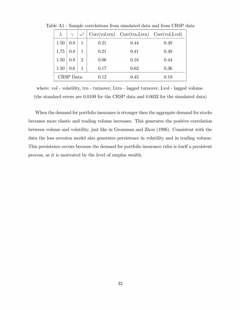
Table A1 - Sample correlations from simulated data and from CRSP data

λ γ ωc Corr(vol,trn) Corr(trn,Ltrn) Corr(vol,Lvol)

1.50 0.8 1 0.21 0.44 0.49

1.75 0.8 1 0.21 0.41 0.49

1.50 0.8 2 0.06 0.18 0.44

1.50 0.6 1 0.17 0.62 0.36

CRSP Data: 0.12 0.45 0.19

where: vol - volatility, trn - turnover, Ltrn - lagged turnover, Lvol - lagged volume.

(the standard errors are 0.0109 for the CRSP data and 0.0032 for the simulated data)

When the demand for portfolio insurance is stronger then the aggregate demand for stocks

becomes more elastic and trading volume increases. This generates the positive correlation

between volume and volatility, just like in Grossman and Zhou (1996). Consistent with the

data the loss aversion model also generates persistence in volatility and in trading volume.

This persistence occurs because the demand for portfolio insurance rules is itself a persistent

process, as it is motivated by the level of surplus wealth.

32

References

[1] Andersen, T. 1996. Return Volatility and Trading Volume: An Information Flow Inter-

pretation of Stochastic Volatility. Journal of Finance 51 (March): 169-204.

[2] Ang, A., Bekaert, G., and Liu, J. 2000. Why Stocks Might Disappoint. Working Paper.

Columbia University, Stanford University and UCLA.

[3] Barberis, N., Huang, M., and Santos, T. 2001. Prospect Theory and Asset Prices.

Quarterly Journal of Economics 116 (February): 1-53.

[4] Basak, S. 1995. AGeneral EquilibriumModel of Portfolio Insurance.Review of Financial

Studies 8 (Winter): 1059-1090.

[5] Basak, S. 2002. A Comparative Study of Portfolio Insurance. Journal of Economic

Dynamics and Control 26 (July): 1217-1241.

[6] Bekaert, G., Hodrick, R. J., and Marshall, D. A. 1997. The Implications of First-Order

Risk Aversion for Asset Market Risk Premiums. Journal of Monetary Economics 40

(September): 3-39.

[7] Benartzi, S., and Thaler, R. H. 1995. Myopic Loss Aversion and the Equity Premium

Puzzle. Quarterly Journal of Economics 110 (February): 73-92.

[8] Benninga, S., and Blume, M. 1985. On the Optimality of Portfolio Insurance. Journal

of Finance 40 (December): 1341-1352.

[9] Berkelaar, A., and Kouwenberg, R., 2001. Optimal Portfolio Choice Under Loss Aver-

sion. Working Paper. Erasmus University Rotterdam.

[10] Bollerslev, T., Chou, R. Y., and Kroner, K. F. 1992. ARCH Modelling in Finance: A

Review of the Theory and Empirical Evidence. Journal of Econometrics 52 (April-May):

5-60.

33

[11] Brock, W., and LeBaron, B. 1996. A Dynamic Structural Model for Stock Return

Volatility and Trading Volume. Review of Economics and Statistics 78 (February): 94-

110.

[12] Campbell, J. Y., Grossman, S. J., and Wang, J. 1993. Trading Volume and Serial

Correlation in Stock Returns. Quarterly Journal of Economics 108 (November): 905-

939.

[13] Epstein, L. G., and Zin, S. E. 1990. First-Order Risk Aversion and the equity premium

puzzle. Journal of Monetary Economics 26 (October): 387-407.

[14] Gallant, R., Rossi P., and Tauchen, G. 1992. Stock Prices and Volume. Review of Fi-

nancial Studies 5 (2): 199-242.

[15] Grinblatt, M., and Keloharju, M. 2000. The Investment Behavior and Performance of

Various Investor Types: A Study of Finland’s Unique Data Set. Journal of Financial

Economics 55 (January): 43-68.

[16] Grinblatt, M., and Keloharju, M. 2001. What Makes Investors Trade. Journal of Finance

56 (April): 589-616.

[17] Grossman, S. J., and Zhou, Z. 1996. EquilibriumAnalysis of Portfolio Insurance. Journal

of Finance 51 (September): 1379-1403.

[18] He, H., and Wang, J. 1995. Differential Information and Dynamic Behavior of Stock

Trading Volume. Review of Financial Studies 8 (4): 919-972.

[19] Heath, C., Huddart, S., and Lang, M. 1999. Psychological Factors and Stock Option

Exercise. Quarterly Journal of Economics 114 (May): 601-628.

[20] Jones, C., Kaul, G., and Lipson, M. 1994. Transactions, Volume and Volatility. Review

of Financial Studies 7 (4): 631-651.

[21] Kahneman, D., and Tversky, A. 1979. Prospect Theory: An Analysis of Decision under

Risk. Econometrica 47 (March): 263-291.

34

[22] Leland, H. E. 1980. Who Should Buy Portfolio Insurance? Journal of Finance 35 (May):

581-594.

[23] LeRoy, S. F., and Porter, R. D. 1981. The Present-Value Relation: Tests Based on

Implied Variance Bounds. Econometrica 49 (May): 555-574.

[24] Lien, D. 2001. A Note on Loss Aversion and Futures Hedging. Journal of Futures Mar-

kets 21 (July): 681-692.

[25] Lien, D., and Wang, Y.Q. 2003. Disappointment Aversion Equilibrium in a Futures

Market. Journal of Futures Markets 23 (February): 135-150.

[26] Locke, P., and Mann, S. 1999. Do Professional Traders Exhibit Loss Realization Aver-

sion. Working Paper. Division of Economic Analysis, Commodity Futures Trading Com-

mission and Neeley School of Business.

[27] Odean, T. 1998. Are Investors Reluctant to Realize Their Losses? Journal of Finance

53 (October): 1775-1798.

[28] Ranguelova, E. 2001. Disposition Effect and Firm Size: New Evidence on Individual

Investor Trading Activity. Working Paper. Harvard University.

[29] Shalen, C. 1993. Volume, Volatility and the Dispersion of Beliefs. Review of Financial

Studies 6 (2): 405-434.

[30] Shefrin, H., and Statman, M. 1985. The Disposition to Sell Winners Too Early and Ride

Losers Too Long: Theory and Evidence. Journal of Finance 40 (July): 777-90.

[31] Shiller, R. J. 1981. Do Stock Prices Move Too Much to be Justified by Subsequent

Dividends? American Economic Review 71 (June): 421-436.

[32] Shiller, R. J. 1998. Human Behavior and the Efficiency of the Financial System. Hand-

book of Macroeconomics: North Holland.

[33] Shleifer, A. 1986. Do Demand Curves for Stocks Slope Down? Journal of Finance 41

(July): 579-590.

35

[34] Shleifer, A. 1999. Inefficient Markets: An Introduction to Behavioral Finance: Oxford

University Press.

[35] Shumway, T. 1997. Explaining Returns with Loss Aversion. Working Paper. University

of Michigan.

[36] Thaler, R. H., and Johnson, E. 1990. Gambling with the House Money and Trying to

Break Even: The Effects of Prior Outcomes on Risky Choice. Management Science 36

(June): 643-660.

[37] Townsend, R. 1983. Forecasting the Forecasting of Others. Journal of Political Economy

91 (August): 546-588.

[38] Tversky, A., Kahneman, D. 1992. Advances in Prospect Theory: Cumulative Represen-

tation of Uncertainty. Journal of Risk and Uncertainty 5 (October): 297-323.

[39] Wang, J. 1993. A Model of Intertemporal Asset Prices Under Asymmetric Information.

Review of Economic Studies 60 (April): 249-282.

[40] Wang, J. 1994. A Model of Competitive Stock Trading Volume. Journal of Political

Economy 102 (February): 127-168.

36

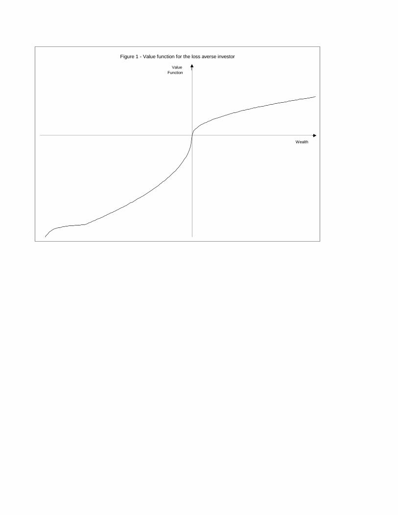
Figure 1 - Value function for the loss averse investor

ValueFunction

Wealth

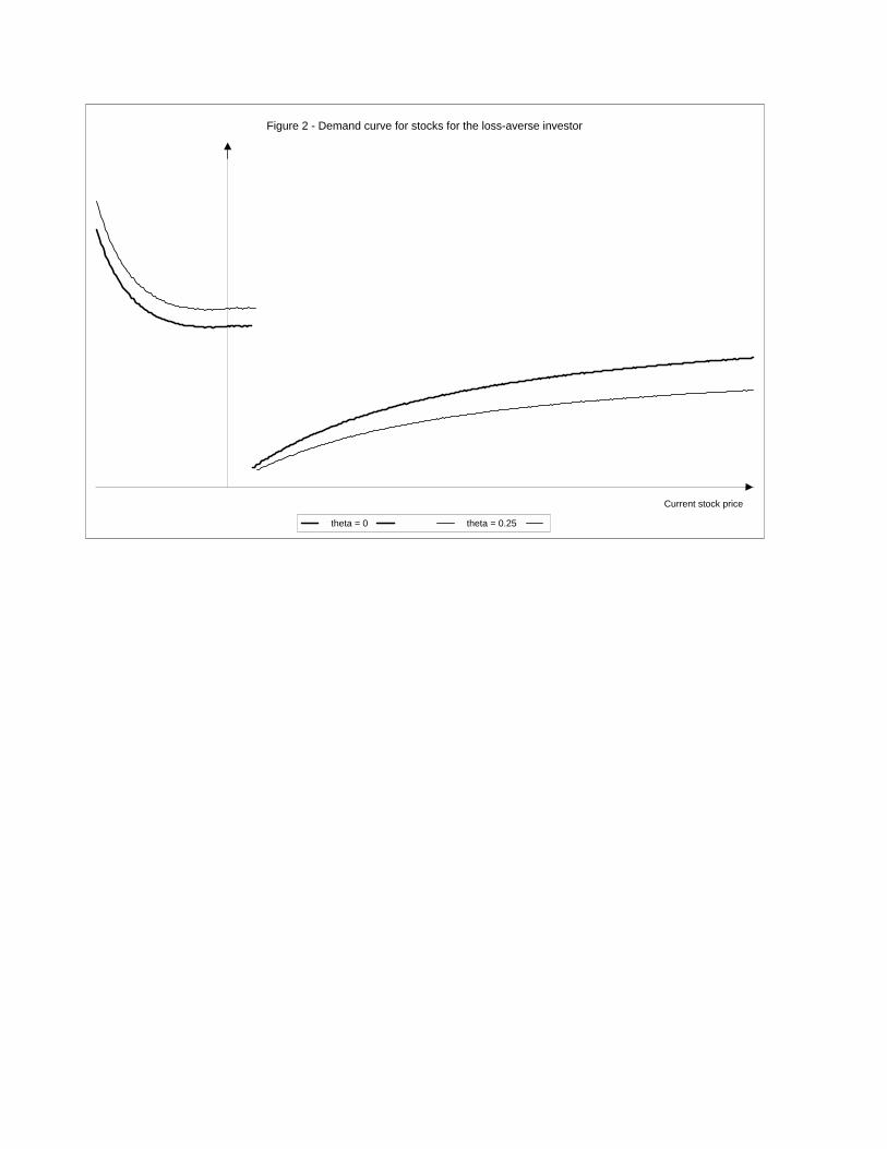
Figure 2 - Demand curve for stocks for the loss-averse investor

Current stock price

theta = 0 theta = 0.25

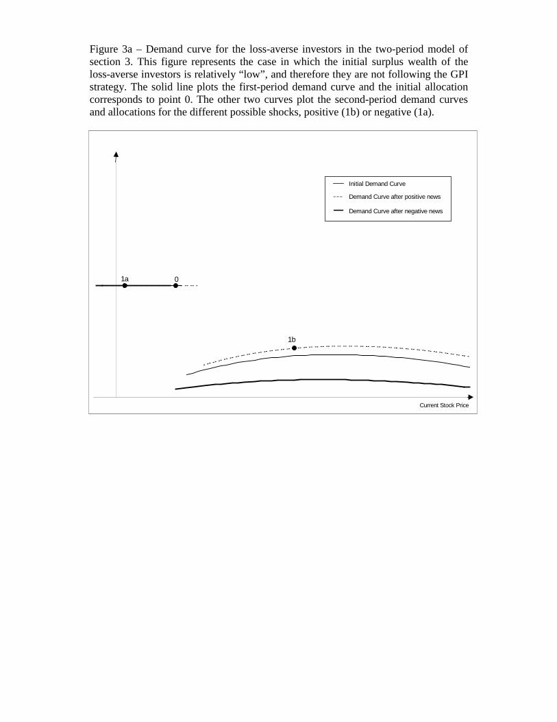
Figure 3a – Demand curve for the loss-averse investors in the two-period model ofsection 3. This figure represents the case in which the initial surplus wealth of theloss-averse investors is relatively “low”, and therefore they are not following the GPIstrategy. The solid line plots the first-period demand curve and the initial allocationcorresponds to point 0. The other two curves plot the second-period demand curvesand allocations for the different possible shocks, positive (1b) or negative (1a).

Current Stock Price

0

1b

1a

Initial Demand Curve

Demand Curve after positive news

Demand Curve after negative news

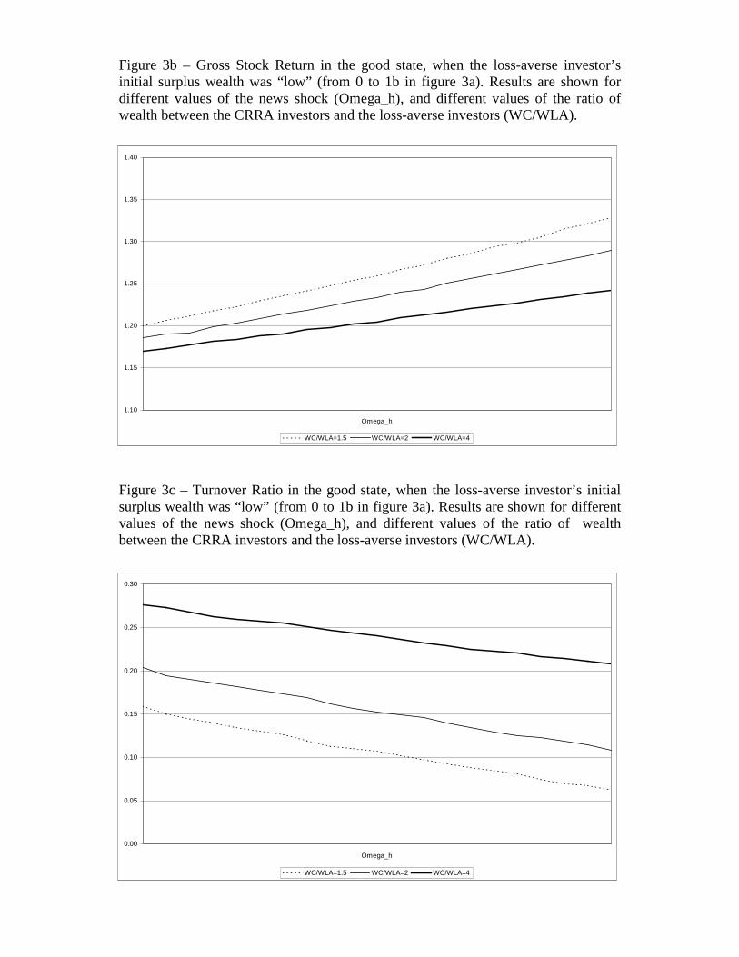
Figure 3b – Gross Stock Return in the good state, when the loss-averse investor’sinitial surplus wealth was “low” (from 0 to 1b in figure 3a). Results are shown fordifferent values of the news shock (Omega_h), and different values of the ratio ofwealth between the CRRA investors and the loss-averse investors (WC/WLA).

Figure 3c – Turnover Ratio in the good state, when the loss-averse investor’s initialsurplus wealth was “low” (from 0 to 1b in figure 3a). Results are shown for differentvalues of the news shock (Omega_h), and different values of the ratio of wealthbetween the CRRA investors and the loss-averse investors (WC/WLA).

1.10

1.15

1.20

1.25

1.30

1.35

1.40

Omega_h

WC/WLA=1.5 WC/WLA=2 WC/WLA=4

0.00

0.05

0.10

0.15

0.20

0.25

0.30

Omega_h

WC/WLA=1.5 WC/WLA=2 WC/WLA=4

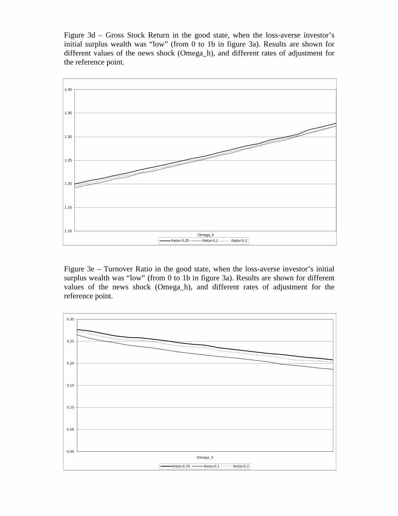
Figure 3d – Gross Stock Return in the good state, when the loss-averse investor’sinitial surplus wealth was “low” (from 0 to 1b in figure 3a). Results are shown fordifferent values of the news shock (Omega_h), and different rates of adjustment forthe reference point.

Figure 3e – Turnover Ratio in the good state, when the loss-averse investor’s initialsurplus wealth was “low” (from 0 to 1b in figure 3a). Results are shown for differentvalues of the news shock (Omega_h), and different rates of adjustment for thereference point.

1.10

1.15

1.20

1.25

1.30

1.35

1.40

Omega_htheta=0.25 theta=0.1 theta=0.2

0.00

0.05

0.10

0.15

0.20

0.25

0.30

Omega_h

theta=0.25 theta=0.1 theta=0.2

Figure 4a – Demand curve for the loss-averse investors in the two-period model ofsection 3. This figure represents the case in which the initial surplus wealth of theloss-averse investors is relatively “high”, and therefore they are following the GPIstrategy. The solid line plots the first-period demand curve and the initial allocationcorresponds to point 0. The other two curves plot the second-period demand curvesand allocations for the different possible shocks, positive (1b) or negative (1a).

Current Stock Price

0

1b

1a

Initial Demand Curve

Demand Curve after positive news

Demand Curve after negative news

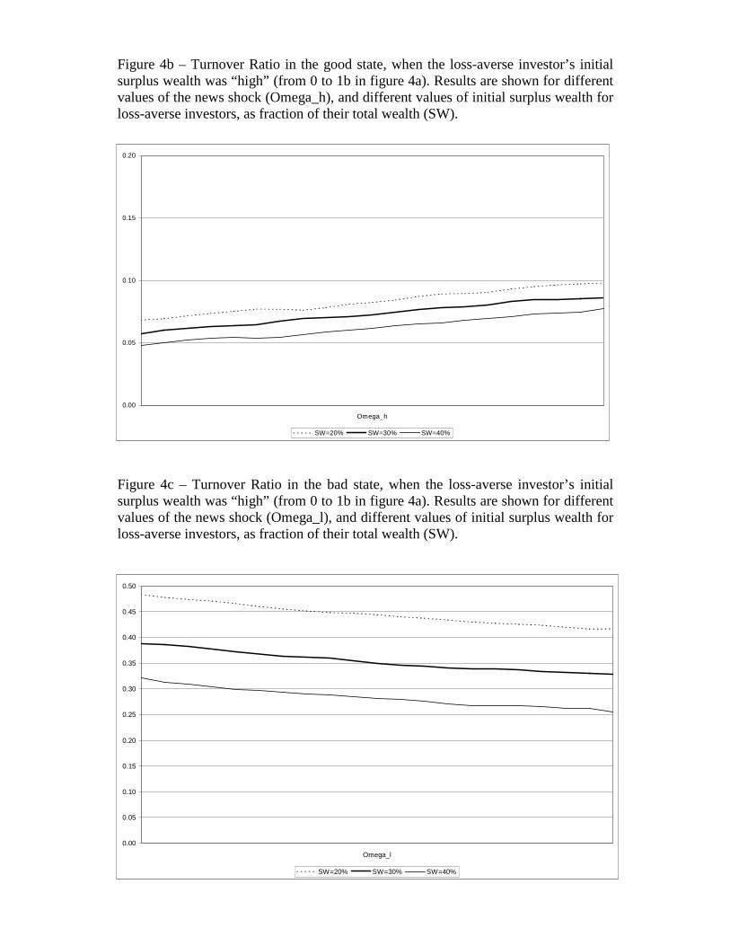
Figure 4b – Turnover Ratio in the good state, when the loss-averse investor’s initialsurplus wealth was “high” (from 0 to 1b in figure 4a). Results are shown for differentvalues of the news shock (Omega_h), and different values of initial surplus wealth forloss-averse investors, as fraction of their total wealth (SW).

Figure 4c – Turnover Ratio in the bad state, when the loss-averse investor’s initialsurplus wealth was “high” (from 0 to 1b in figure 4a). Results are shown for differentvalues of the news shock (Omega_l), and different values of initial surplus wealth forloss-averse investors, as fraction of their total wealth (SW).

0.00

0.05

0.10

0.15

0.20

Omega_h

SW=20% SW=30% SW=40%

0.00

0.05

0.10

0.15

0.20

0.25

0.30

0.35

0.40

0.45

0.50

Omega_l

SW=20% SW=30% SW=40%