Pole -PlacementDesign

& State Observer

Presented by:-

Er. Sanyam S. Saini

ME(I&C) Regular

Outlines

• Servo Design: Introduction of the

reference Input by Feed forward Control

• State Feedback with Integral Control

Servo Design: Introduction of the

Reference Input by Feed Forward Control

The characteristics Equation of the Closed –Loop Control System is chosen so as to give satisfactory Transient to disturbances.

However, no mention is made of a reference i/p or a design consideration to yield good transient response with respect to command changes.

In general, both of these considerations should be taken into account in the designing of control system.

This can be done by the proper introduction of the references i/p into the system equations.

bu(t) +Ax(t)=(t)x

kx(t)- =u(t)

r=cxs

Consider the completely controllable SISO LTI system with nth – order state variable model

We assume that all the n state variables can be accurately measured at all times. Implementation of appropriately designed Control Law of the form.

cx(t) =y(t)

Let us now assume that for the system given by equs.(i & ii), the desired steady- state value of the controllable variable y(t) is a constant reference input r. For this servo system, the desired equilibrium state is a constant point in state space & is governed by the equations.

…………….…………………(i)

…………….…..………….…(ii)

sx

…………….…..………………………………(iii)

Continued…….

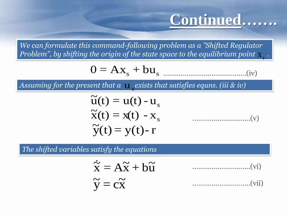
sx- x(t)=(t)x~

r -y(t) =(t)y~

u~b +x~A =x~

x~c=y~

ss bu +Ax=0

su-u(t)=(t)u~

Continued…….

We can formulate this command-following problem as a ”Shifted Regulator Problem”, by shifting the origin of the state space to the equilibrium point .

sx

…………….………..………….…(iv)

suAssuming for the present that a exists that satisfies equns. (iii & iv)

.………..………….…..(v)

The shifted variables satisfy the equations

.………..……………...(vii)

.………..………….…..(vi)

su

0)(bk)x-(A s ss kxub

)()(x 1

sss kxubbkA

x~-k=u~

)()(cx 1

s ss kxubbkAcr

Nr)kx(u ss

Continued…….

This system possesses a time – invariant asymptotically stable control law

In terms of the original state variables , total control effort

or

The equation has a unique solutions for ; )( ss kxu

.………..………….…..(x)

.………..………….…..(viii)

skxsu -kx(t)u(t) .………..….……….…..(ix)

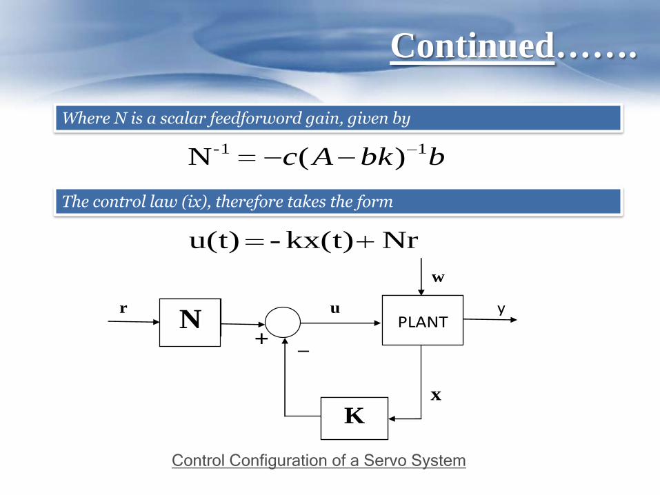
Nrkx(t)- u(t)

w

r u y

+ _

x

N

PLANT

K

Control Configuration of a Servo System

bbkAc 1-1 )(N

Continued…….

The control law (ix), therefore takes the form

Where N is a scalar feedforword gain, given by

Numerical Problem

Consider a Attitude Control System for a rigid satellite . Design the control Configuration for the give control system as given follows. (Previous example taken in stability improvement by state feedback)

Solution:-

The Plant equations are,

1

0b

00

10A

bu(t) +Ax(t)=(t)x

cx(t) =y(t)

Where

01c

Herex1(t)= Position x2(t)= Position )(t )(t

Continued…….

As the plant has integrating property, the steady- state value of the i/p must be zero(otherwise o/p cannot stay constant).

The reference i/p is a step function. The desired steady-state is,

For this case, the shifted regulator problem may be formulated as follows,

rrT

rsx 0

su

rxx 11~

22~ xx

Shifted regulator variables satisfy the equations.

u~b +x~A =x~

The state – feedback control

kx(t)- =u(t)

Continued…….

Therefore ,

x~bk)-(A =x~

As in previous example, we found eigenvalues of are placed at the desired location when,

bk)-(Aj44-

832kk 21 k

The control law expressed in terms of the original state variables is given as,

rkxkxkxkxku 122112211~~

rkkx 1

Continued…….

The control configuration for attitude control of the satellite is showing as following,

r

Attitude Control of a Satellite

State Feedback with Integral Control

For the system bu(t) +Ax(t)=(t)x

cx(t) =y(t)

Need of state feedback with integral control:

The control configuration of previous problem produces a generalization of Proportional & Derivative feedback but it dose not include integral control unless special steps are taken in the design process.

We can feedback the state “x” as well as the integral of the error in output

by augmenting the plant state “x” with extra “integral state” z,

defined by the equation t

0

r)dt-(y(t)z(t)……….………….…(i)

Continued…….Since z(t) satisfies the differential equation,

rtcxrty )()((t)z ……….………….…(ii)

It is easily included by augmenting the original system as follows:

rub

z

x

c

A

z

x

1

0

00

0

Since “r” is constant, in the steady – state , provided that the system is stable.

0,0 zx

This means that the steady -state solutions & must satisfy the equation

ss zx , su

s

s

su

b

z

x

c

Ar

00

0

1

0

……….………….…(iv)

……….………….…(iii)

Continued…….Therefore,

From equation (iii) & (iv)

)(00

0s

s

suu

b

zz

xx

c

A

z

x

….………….…(v)

Now define new state variables as follows , representing the deviations from the steady - state:

s

s

zz

xxx~

)(~suuu

In terms of these variables,

….………….…(vi)

ubxAx ~~~….………….…(vii)

Continued…….Where,

0

0

c

AA

0

bb

The significance of this result is that by defining the deviation from steady-state as state & control variables,

The design problem has been reformulated to be the Standard regulator problem with as the desired state.0~x

We assume that an asymptotically stable solution to this problem exists & is given by-

x~-k=u

Partitioning “k” appropriately & using eqns. (vi)

][ ip kkk

Continued…….

s

s

ipszz

xxkkuu

)()( sisp zzkxxk

The steady-state terms must balance, therefore

t

ipip dtrtykxkzkxku0

))((

The control, thus consist of proportional state feedback & integral control of output error.

At steady-state, ; thereforeox~

0)(limt

tz rty )(limt

or

Thus, by integrating action , the output “y” is driven to the no- offset condition. This will be true even in the presence of constant disturbances acting on the plant.

Continued…….

ik

pk

r

w

u y

x

State feedback with integral control

Numerical Problem

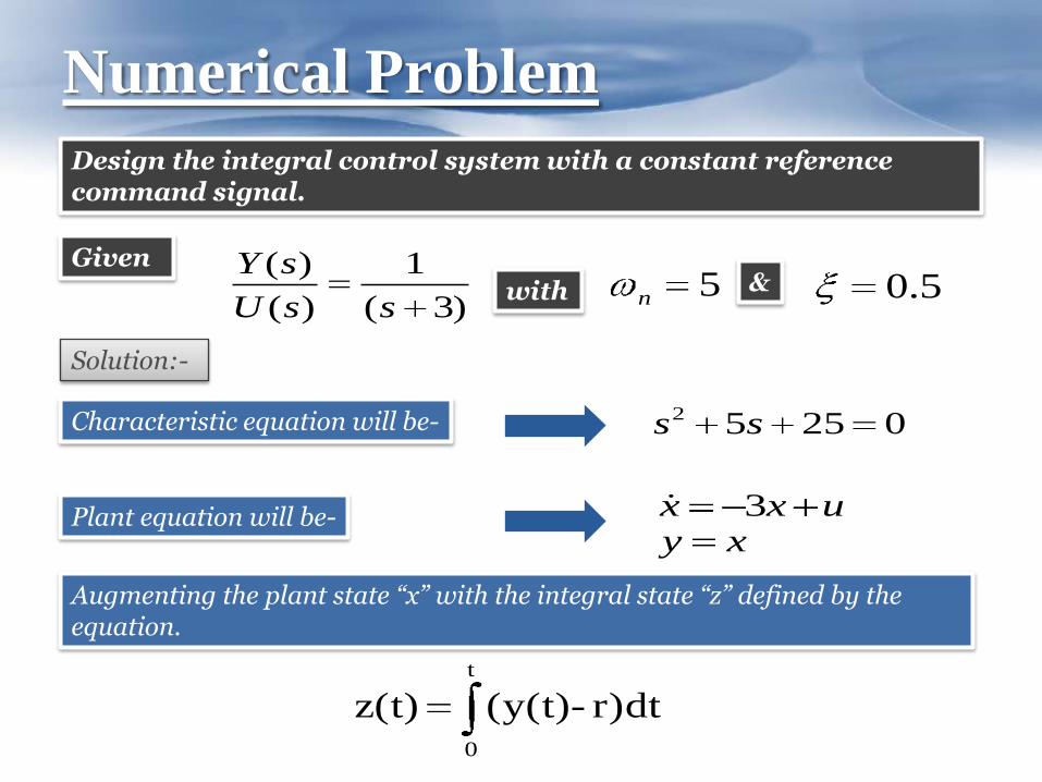
Design the integral control system with a constant reference command signal.

Given

)3(

1

)(

)(

ssU

sY5n 5.0&with

Solution:-

Characteristic equation will be- 02552 ss

Plant equation will be- uxx 3xy

Augmenting the plant state “x” with the integral state “z” defined by the equation.

t

0

r)dt-(y(t)z(t)

Continued…….

ruz

x

z

x

1

0

0

1

01

03

We get

Since

s

s

zz

xxx~

)(~suuu

State equation becomes uxx ~

0

1~

01

03~

Continued…….

We can find “k” from

2550

1

01

03det 2 ssksI

255)3( 2

21

2 ssksksAfter solving

Therefore ][252 ip kkk

The control

t

ip dtrtyxzkxku0

))((252

Continued…….

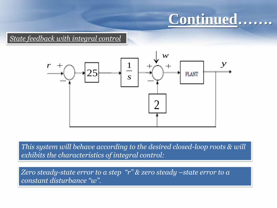
r yw

25 s

1

2

State feedback with integral control

This system will behave according to the desired closed-loop roots & will exhibits the characteristics of integral control:

Zero steady-state error to a step “r” & zero steady –state error to a constant disturbance “w”.

Thank You