1

Pilot Assignment Schemes for Cell-Free

Massive MIMO Systems

Priyabrata Parida and Harpreet S. Dhillon

Abstract

In this work, we propose three pilot assignment schemes to reduce the effect of pilot contamination

in cell-free massive multiple-input-multiple-output (MIMO) systems. Our first algorithm, which is based

on the idea of random sequential adsorption (RSA) process from the statistical physics literature, can be

implemented in a distributed and scalable manner while ensuring a minimum distance among the co-pilot

users. Further, leveraging the rich literature of the RSA process, we present an approximate analytical

approach to accurately determine the density of the co-pilot users as well as the pilot assignment

probability for the typical user in this network. We also develop two optimization-based centralized

pilot allocation schemes with the primary goal of benchmarking the RSA-based scheme. The first

centralized scheme is based only on the user locations (just like the RSA-based scheme) and partitions

the users into sets of co-pilot users such that the minimum distance between two users in a partition

is maximized. The second centralized scheme takes both user and remote radio head (RRH) locations

into account and provides a near-optimal solution in terms of sum-user spectral efficiency (SE). The

general idea is to first cluster the users with similar propagation conditions with respect to the RRHs

using spectral graph theory and then ensure that the users in each cluster are assigned different pilots

using the branch and price (BnP) algorithm. Our simulation results demonstrate that despite admitting

distributed implementation, the RSA-based scheme has a competitive performance with respect to the

first centralized scheme in all regimes as well as to the near-optimal second scheme when the density

of RRHs is high.

Index Terms

Random sequential adsorption, cell-free massive MIMO, max-min algorithm, pilot assignment,

spectral graph theory, branch and price.

I. INTRODUCTION

The concept of distributed implementation of MIMO technique has been actively explored

for more than a decade. Recent push towards network densification has also made its practical

Authors are with Wireless@VT, Dept. of Electrical and Computer Engineering, Virginia Tech, Blacksburg, VA (Email:

{pparida, hdhillon}@vt.edu). The support of the US NSF (Grant ECCS-1731711) is gratefully acknowledged. This paper was

presented in part at the IEEE Globecom, 2019 [1].

arX

iv:2

105.

0950

5v1

[cs

.IT

] 2

0 M

ay 2

021

2

implementation viable. In a distributed MIMO network, a number of geographically separated

RRHs simultaneously serve users in the network and are connected to a central base band unit

(BBU), which performs the physical layer tasks of symbol detection and decoding along with

complex upper layer tasks such as resource scheduling. In a dense network, the access points (or

RRHs) can be leveraged for distributed implementation resulting in higher SE through macro-

diversity and elimination of frequent handovers as users move from one access point to another.

Apart from network densification, massive MIMO (mMIMO) is also one of the major enablers

of the 5G wireless networks. Hence, it is natural to study the performance of a wireless network

where a large number of RRHs with multiple antennas simultaneously serve multiple users.

Not surprisingly, such studies have been conducted over the years under different pseudonyms

such as network MIMO, coordinated multi-point [2], cloud radio access network (RAN) [3],

fog-mMIMO [4], and recently the cell-free mMIMO [5], [6]. Successful implementation of any

MIMO technique requires accurate channel state information (CSI) at the transmitter (or receiver).

Similar to cellular mMIMO networks, the CSI acquisition in cell-free mMIMO systems needs to

be done through uplink pilot transmission due to its scalability. However, under the assumptions

of independent Rayleigh fading and sub-optimal linear precoders, pilot contamination becomes

the only capacity limiting factor of both cellular and cell-free mMIMO networks [6]–[8]. Hence,

judicious pilot assignment is essential to reduce the effect of pilot contamination, which is the

main focus of this paper.

A. Related works

In general, the optimal pilot assignment problem for a cell-free massive MIMO system is non-

deterministic polynomial-time (NP)-hard in nature. Hence, the computational resources required

to obtain the optimal solution scale exponentially with the number of users. Therefore, almost

all the works in the literature focus on providing heuristics-based algorithms to get an efficient

solution. These algorithms can be broadly categorized into centralized and distributed schemes.

In [6], a distributed random pilot allocation and a centralized greedy pilot allocation schemes are

presented for a cell-free mMIMO network. In [4] and [9], a distributed random access type pilot

assignment scheme is proposed, where a user is not served if its channel state information (CSI)

cannot be estimated reliably. A centralized structured pilot allocation scheme with an iterative

application of the K-means clustering algorithm is presented in [10]. A natural way to address the

resource allocation problem is through graph theoretic framework. This idea has been explored

3

in [11]–[13]. In [11], a centralized pilot sequence design scheme is proposed where the users in

the neighborhood of an RRH use orthogonal pilot sequences. The problem is posed as a vertex

coloring problem and solved using the greedy DASTUR algorithm. Along the similar lines, the

authors of [12] construct the conflict graph by having an edge between users that are dominant

interferers to each other. The graph coloring problem is solved using a greedy algorithm. In [13],

the pilot assignment problem is mapped to the Max K-cut problem, which is solved using a

heuristic algorithm. In [14], a dynamic pilot allocation approach is presented where two users

can be assigned the same pilot sequence if the signal to interference and noise ratios (SINRs) of

both the users are above a certain threshold. While the aforementioned works primarily focus

on reducing the interference due to pilot contamination, authors in [15] and [16] solve pilot

allocation optimization problems to maximize certain utility metrics. Due to the NP-hard nature

of the problem, authors in [15] use the Tabu search to solve the pilot allocation problem with

the objective of maximizing sum-user SE. Further, in [16], system throughput maximization, and

minimum user throughput maximization problems are solved using an iterative scheme based

on the Hungarian algorithm. Most of these works rely on the common underlying principle that

the same pilot can be assigned to the users that have sufficient geographical separation. This

principle also motivates the main pilot assignment scheme proposed in this work along with the

additional objective that it should be distributed as well as scalable in nature while providing

competitive performance in terms of average user SE. Our contributions are summarized next.

B. Contributions

1. Random sequential adsorption (RSA)-based pilot assignment scheme: First, we propose

a random pilot assignment algorithm with a minimum distance constraint among the co-pilot

users to reduce the effect of pilot contamination. The algorithm is inspired by random sequential

adsorption (RSA) process, which has been traditionally used across different scientific disciplines

such as condensed matter physics, surface chemistry, and cellular biology, to name a few, to

study the adsorption of large-particles such as colloids, proteins, and bacteria on a surface. Apart

from proposing the algorithm with a potential distributed implementation in the network, our

contribution lies in the accurate analytical characterization of the density of co-pilot users for a

given total user density and a minimum distance threshold. This result is used to characterize

the probability of a pilot assignment to the typical user in the network.

4

2. Two centralized pilot allocation schemes for benchmarking: To quantify the efficacy of the

proposed RSA-based pilot allocation scheme, we also propose two centralized algorithms. The

first algorithm, similar to the RSA scheme, is agnostic to the RRH locations and considers only

the user locations. This algorithm, named the max-min distance-based algorithm, partitions the

users into sets of co-pilot users to maximize the minimum Euclidean distance among the co-pilot

users. This scheme is optimal from the perspective of geographical separation between a set of

co-pilot users. In the proposed algorithm, the minimum distance is obtained through the bisection

search subject to a set of feasibility constraints. The second algorithm, which takes into account

both RRH and user locations, maximizes the sum-user SE of the network subject to minimum

user SINR constraint. First, leveraging tools from spectral graph theory, the algorithm partitions

the users into a desired number of clusters based on similar path-loss with respect to the RRHs.

Next, using the BnP algorithm, sets of co-pilot users are obtained with the additional constraint

that two users in the same cluster are not assigned the same pilot. This approach provides

us with a near-optimal solution in terms of sum-user SE at the cost of a significant increase in

computational complexity compared to the other two algorithms. Therefore, it is more suitable to

use this algorithm for benchmarking other pilot allocation schemes than practical implementation.

3: Insights from numerical results: Through extensive system simulation, we conclude that

the RSA-based pilot allocation scheme provides competitive performance compared to the max-

min distance-based pilot allocation scheme, especially when the ratio of the number of users

to the pilots is relatively low. Further, the RSA-based scheme achieves close to near-optimal

performance with the increasing RRH density. In addition, we compare the performance of the

RSA and the max-min schemes to another centralized pilot allocation scheme based on the

iterative K-means algorithm available in the literature. While RSA performs as well as the K-

means, the max-min distance-based scheme marginally outperforms it. Despite being a distributed

scheme, the competitive performance of the RSA-based scheme compared to other centralized

schemes makes it an attractive alternative for system implementation.

II. SYSTEM MODEL

A. Network model

We limit our attention to the downlink (DL) of a cell-free mMIMO system. The locations of

the RRHs form a Poisson point process (PPP) Φr of density λr. Similarly, the user point process

Ψu is also modeled as an independent PPP of density λu. Each RRH is equipped with N antennas

5

and each user with a single antenna. The RRHs are connected to a BBU and collectively serve

users in the network. The distance between a user at uk ∈ Ψu and an RRH at rm ∈ Φr is

denoted by dmk. In line with the mMIMO literature, where the number of antennas is assumed

to be an order of magnitude more than the number of users, we consider that the antenna density

Nλr � λu. Further, invoking stationarity of this setup, we analyze the system performance for

the typical user uo, which is located at the origin o.

Channel estimation: Let gmk =√βmkhmk be the channel gain between the m-th RRH and

the k-th user, where βmk captures the large-scale channel gain and hmk ∼ CN (0, IN) captures

the small-scale channel fluctuations. We consider that the large-scale channel gain βmk is only

due to the distance dependent path-loss, i.e. βmk = l(dmk)−1, where l(·) is a non-decreasing

path-loss function. While the analysis presented in this paper is agnostic to the choice of l(·),

we will need to choose a specific l(·) for the numerical results, which is presented in Section VI.

In order to obtain the channel estimates, each user uses a pilot from a set of P orthogonal

pilot sequences P = [p1,p2, . . . ,pP ]T , where pi denotes the i-th sequence. The length of each

pilot is τp symbol durations, which is less than the coherence interval. Since we assume that the

P sequences are orthogonal to each other, P ≤ τp and pHi pj = τp1(i = j), where 1(·) denotes

the indicator function. Due to finite number of pilots, the pilot set needs to be reused across the

network. Let the pilot used by the k-th user be p(k). During the pilot transmission phase, the

received signal matrix Ym ∈ CN×τp at the m-th RRH is

Ym = τp∑

uk∈Ψu

gmkp(k)T +Wm,

where ρp is the normalized transmit signal-to-noise ratio (SNR) of each pilot symbol and Wm is

an additive white Gaussian noise matrix whose elements follow CN (0, 1). At the m-th RRH,

the least-square estimate, yml ∈ CN×1, of the channel of the users that use the l-th sequence is

yml = Ymp∗l = τpρp

∑uk∈Φul

gmk +Wmp∗l ,

where Φul is the set of users that use the l-th sequence. Further, the set of users that are assigned

a pilot is defined as Φu = ∪Pk=1Φuk. Assuming uo ∈ Φul, the minimum-mean-squared-error

(MMSE) estimate of the channel of the typical user at the m-th RRH is given as

gmo = E[ymlgHmo](E[ymly

Hml])

−1yml =βmo∑

uk∈Φul

βmk + 1τpρp

yml = αmoyml. (1)

6

In this case, the error vector gmk = gmk − gmk is uncorrelated to the estimated vector. Now the

estimate and the error vectors are distributed as follows [5]:

gmo ∼ CN (0, γmoIN) , gmo ∼ CN (0, (βmo − γmo) IN) ,

where γmo = τpρpβ2mo

1+∑

uk∈Φulτpρpβmk

. From the expression of γmo, it is clear that the quality of channel

estimates depend on the locations of the co-pilot users in Φul.

DL user SINR: Using the channel estimates, each RRH precodes the data for all the users

in the network. In this work, we consider conjugate beamforming precoding scheme. Since the

m-th RRH cannot distinguish among the channels of the users that use the l-th pilot, it uses the

normalized direction of yml for beamforming, i.e. the precoding vector used to transmit data to

the users that use l-th pilot is given as

wml = yml/√

E[‖yml‖2] = gmo/√

E[‖gmo‖2].

Now the data transmitted by the m-th RRH is given as

xm =√ρd

P∑p=1

w∗mp∑

uk∈Φup

√ηmkqk,

where ηmk is the transmission power used by the m-th RRH for the k-th user and qk ∼ CN (0, 1)

is the transmit symbol of the k-th user. For each RRH, we assume the following power constraint:

E[‖xm‖2] ≤ ρd. The symbol received at o (that uses the l-th pilot) is given as

ro =∑

rm∈Φr

gTmoxm + no =√ρd∑

rm∈Φr

(gTmo + gTmo)g∗mo√Nγmo

√ηmoqo

+√ρd

P∑p=1,p 6=l

∑uk∈Φup

∑rm∈Φr

gTmog∗mp√Nγmp

√ηmkqk

+√ρd

∑uk′∈Φ′ul

∑rm∈Φr

(gTmo + gTmo)g∗mo√Nγmo

√ηmk′qk′ + no,

where Φ′ul = Φul \ uo, the first term on the right hand side is the desired term, the second term

corresponds to multi-user interference due to non-copilot users, and the third term is the source

of interference due to pilot contamination.

B. Metrics for system performance analysis

1) DL power control and SINR of an arbitrary user: Since our objective is to propose a scheme

to reduce pilot contamination, we focus on the operational regime where pilot contamination

7

dominates rest of the interference terms. In the following lemma, we present the SINR expression

of the typical user under the assumption that the RRHs are equipped with N →∞ antennas.

Lemma 1. Conditioned on Φr and Φu, the asymptotic SINR of the typical user is given as

SINRo,∞ =

(∑rm∈Φr

√ηmoγmo

)2∑uk∈Φ′ul

(∑rm∈Φr

√ηmkγmo

)2 . (2)

Proof: The estimated symbol at the typical user can be obtained as qo = ro/√N. Now,

using the law of large numbers, as N → ∞, gTmog

∗mo

N→ γmo,

gTmog

∗mo

N→ 0, and gT

mog∗mp

N→ 0.

Hence, the limiting SINR converges to (2).

In this work, we consider a distributed power control scheme [10] where the transmission

power used by the the m-th RRH for the typical user at o is given as

ηmo =γmo

P∑

uk∈Φulγmk

, (3)

such that∑

uk∈Φulηmk = 1/P . We assume that the RRHs allocate equal power 1/P to serve

each set of co-pilot users. Now, we define the following metrics for the performance analysis:

i. Pilot assignment probability of the typical user: Since the RSA-based pilot assignment is

stochastic in nature, for a given realization of user locations, a few of the users may not be

assigned a pilot. Hence, pilot assignment probability to the typical user is an important metric

to analyze for this scheme. Let {Io = 1} be the event that the user at o is assigned a pilot. Then

the aforementioned probability is given as

Mo = P[Io = 1] = E[1(Io = 1)], (4)

where the expectation is taken over Ψu. In Section III-A, we present our proposed approach to

characterize the above quantity along with the RSA-based pilot assignment scheme. This quantity

can be used to get an estimate of the number of pilots necessary to satisfy target pilot assignment

probability for a given user density. Note that Mo = 1 for the max-min distance-based and the

BnP-based schemes proposed in this work.

ii. Average user spectral efficiency: It is defined as

SEo =E [Io log2(1 + SINRo)] = E[log2(1 + SINRo)

∣∣Io = 1]P[Io = 1], (5)

where the expectation is taken over Φr,Ψu.

8

iii. Sum-user spectral efficiency: In contrast to the above two quantities, sum-user SE is defined

for a given realization of Φr and Ψu over a finite observation window W ⊂ R2 and given as

ΣSE =∑

uj∈Ψu∩W

Ij log2(1 + SINRj), (6)

where Ij = 1 for the max-min and BnP-based schemes and Ij ∈ {0, 1} for the RSA-based

scheme.

III. RSA-BASED PILOT ALLOCATION SCHEME

Before delving into the proposed RSA-based pilot assignment scheme, we find it pertinent to

mention the complexity associated with pilot assignment problem that serves as a motivation to

propose a heuristic algorithm. The objective of any resource allocation algorithm is to maximize

a cost (reward) function subject to certain constraints due to a limited availability of resources.

In our case, we choose the cost function to be the sum SE. Hence, for a given realization

of the locations of RRHs and users, our objective is to maximize the sum SE by judiciously

selecting the set of co-pilot users. Inspired by the column generation approach prevalent in the

linear programming literature, the problem can be formulated in the following way. We consider

each potential set of co-pilot users as a column. In order to have a finite dimension for the

set of feasible solutions, it is imperative to consider a finite observation window with Nu users

S = {u1,u2, . . . ,uNu} and Nr RRHs. Let A denotes the set of all the potential co-pilot user

sets avoiding the null and singleton sets. Hence, the cardinality of A, which is also the total

number of columns, is 2Nu −Nu− 1. As an example, consider a set of users Ak = {u1,u2,u3}.

The corresponding column for these co-channel users is given as xk =[1 1 1 0 . . . 0

]T∈

{0, 1}Nu . We define the matrix A, where each column corresponds to a set in A. Further, the

cost of a set Aj (equivalently, the cost of the j-th column xj) is given as

c(xj) =

∑

ui∈Ajlog2 (1 + Γij) , if Γij ≥ Γmin ∀ui ∈ Aj

−M, if Γij < Γmin for any ui ∈ Aj(7)

where the SINR of the i-th user in the j-th set is Γij =(∑

rm∈Φr

√ηmiγmi)

2∑uk∈{Aj\ui}(

∑rm∈Φr

√ηmkγmi)

2 , Γmin is

the minimum SINR threshold, and M is a large positive number. With this definition the set

of co-pilot users not satisfying the minimum SINR threshold even for a single user is (almost)

never selected. Now, we express the optimization problem as

maxΛ

|A|∑s=1

c(xs)λs (8a)

9

s.t. AΛ = 1 (8b)

‖Λ‖1 = P (8c)

Λ ∈ {0, 1}|A|, (8d)

where Λ =[λ1, λ2, . . . , λ|A|

]T , (8b) ensures that each user is assigned exactly one pilot, (8c)

ensures that P columns are selected each representing a set of co-pilot users. Above problem

is NP-hard. Further, the feasible solution space of the problem is(|A|P

). Hence, if we wish to

obtain the optimal solution even for a moderately small system of 24 users with 6 pilots, we

need to search over a feasible set of size approximately 3.1× 1040.

Owing to the complexity of the problem, it is natural to consider heuristic solutions, albeit

sub-optimal, that can be implemented efficiently in the network. In the following subsection, we

present a sub-optimal pilot allocation algorithm that only considers user locations to select the

set of co-pilot users such that the pilot contamination-based interference is mitigated thereby

implicitly improving the user SE as well as the sum SE. This algorithm, which is inspired by

the RSA process, can be implemented both in a centralized or distributed manner and is easily

scalable as the network size grows.

A. RSA-based pilot assignment algorithm

Our goal is to select the sets of co-pilot users among all the users in the network such

that a minimum distance Rinh is maintained between two co-pilot users. This can be achieved

by dependent selection of the users from the original user point process Ψu as outlined in

Algorithm 1. The algorithm assigns a random mark tk, which is uniformly distributed in [0, 1],

to each point uk ∈ Ψu. Let BRinh(uk), a circle of radius Rinh centered at uk, be defined as the

contention domain of the point at uk. For pilot assignment, the algorithm considers each user

in increasing order of their marks, i.e. the lowest mark is considered first. From the available

set of pilots, a pilot is randomly assigned to a user at uk, where the set of available pilots

are those which have not been assigned to the users in BRinh(uk). Note that to implement this

algorithm, the BBU requires only the location information of the users, which does not require

any additional signaling overhead as this information is typically present at a centralized node

in the network such as the BBU. At the end of this subsection, we also discuss a protocol for

potential distributed implementation of the algorithm.

10

Input: User locations Ψu, the set of pilots P , inhibition distance Rinh

Result: Pilot assignment table TInitialization: T = ∅, a random mark ti ∼ U(0, 1) for each ui ∈ Ψu;Let Ψu be the set of users in the increasing order of marks;for User u ∈ Ψu do

Set: P ′ = P;while User u is not assigned a pilot do

if P ′ == ∅ thenNo pilot can be assigned: T = T ∪ ∅;Break;

else

Select a pilot sequence pk randomly from the set P ′;

endif No other users in BRinh

(u) are using pk thenAssign the pilot: T = T ∪ pk;Break;

else

Remove pk from list of potential pilots: P ′ = P ′ \ pk;

endend

end

Algorithm 1: The RSA-based pilot assignment algorithm in for a cell-free mMIMO system.

Fig. 1: Realizations of co-pilot user locations using Algorithm 1. Parameters: Rinh = 200, λu = 2× 10−6 (left), λu = 10−3

(center, right). Left and center figures represent realizations of co-pilot users for P = 1. Right figure represents a realization of

co-pilot users for P = 2.

For the system designers, it is useful to know the probability that a user will be scheduled as

a function of the density of users and the number of pilots in the system. Following subsections

present an approximate theoretical result that answers the aforementioned question eliminating

the need for a system simulation. It is worth-mentioning that the approximate result is a new

contribution to the RSA literature as the exact solution for counterpart of this problem even in

the case of 1D is unknown.

1) Analysis of the pilot assignment probability: Recall that Φu is the set of users that are

assigned a pilot (in this case by Algorithm 1), i.e. Φu = ∪Pp=1Φup. Let to be the mark associated

11

with the typical user. Now, the user at o is assigned a pilot if |Φu ∩ BRinh(o)| ≤ P − 1. This is

ensured by the following two events:

• E1: there are at most P − 1 points in BRinh(o) ∩Ψu that have marks less than to,

• E2: there are more than P −1 points in BRinh(o)∩Ψu that have marks less than to. However,

some of these points are not assigned a pilot as their contention domains have more than

P points with marks smaller than their respective marks.

While obtaining the probability of E1 is straightforward, characterizing E2 is highly non-trivial

even for P = 1. Note that for P = 1, the above formulation has been used to model the

CSMA-CA networks. However, due to the intractability of E2, Matern hardcore process of type-

II (MHPP-II) has been used for approximate characterization for Φu [17]. Hence, one may be

inclined to extend the MHPP-II process for P ≥ 2. However, one of the limitations of the

MHPP-II process is that it underestimates the number of points in Φu [18]. Hence, the extension

of the MHPP-II model for P ≥ 2 will not result in an accurate estimation. On the other hand,

for P = 1, Φu is exactly modeled by the simple sequential inhibition (SSI) process [18] or the

RSA process [19]. Using this fact, in the sequel, we present an efficient heuristic to estimate the

pilot assignment probability.

Consider a finite observation window BRs(o) ⊂ R2, where Rs � Rinh. Let Nu = |Ψu∩BRs(o)|

be the total number of users and Ns = |Φu ∩ BRs(o)| be the number of users that are assigned

a pilot. Note that for a given Nu, Ns is a random variable as it depends on the realization of

Ψu as well as random marks associated with these points. Now, for a given Nu > P , E[Ns|Nu]

is the average number of users that are assigned a pilot. Hence, the probability that the typical

user out of the Nu users is assigned a pilot is E[Ns|Nu]/Nu. On the other hand, for Nu ≤ P ,

the typical user is assigned a pilot with probability 1. Combining these two events, we write the

pilot assignment probability as

P[Io = 1] =P [Nu ≤ P ] + ENu [E[Ns|Nu]N−1u

∣∣Nu > P ]P [Nu > P ]

≈P [Nu ≤ P ] + E[Ns|Nu = πR2

sλu]E[N−1

u

∣∣Nu > P ]P [Nu > P ] , (9)

where the second step is an approximation as instead of ENu [E[Ns|Nu]|Nu > P ], we determine

E[Ns] by considering Nu = πR2sλu, which is its expected value. Since Nu is Poisson distributed

with mean λuπR2s ,

E[N−1u |Nu > P

]=λuπR

2s −

∑Pn=0 Poi(λuπR2

s, n)

1−∑P

n=0 Poi(λuπR2s, n)

, (10)

12

where Poi(λuπR2s, n) = e−λuπR

2s

(λuπR2s)n

n!.

Next, we discuss our approach to analytically estimate E [Ns|Nu = πR2sλu] leveraging the rich

theory of the RSA process. For convenience, we use the notation E [Ns] to represent the above

expectation. We first present the analysis for the special case of P = 1 followed by its extension

to the general case of P ≥ 2.

2) Pilot assignment probability for P = 1: Traditionally, the RSA process has been used

across different disciplines, such as condensed matter physics, surface chemistry, and cellular

biology, to study the adsorption of different substances, such as colloids, proteins, and bacteria,

on a surface [19]. Next, we present a brief overview of the RSA process before analyzing pilot

assignment probability.

Random sequential adsorption process: An RSA process is defined as a stochastic space-time

process, where n-dimensional hard spheres sequentially arrive at random locations in Rn such

that any arriving sphere cannot overlap with already existing sphere. More formally, for 2D case,

let Ψ be a homogeneous space-time point process on R2×R+. The circles with radii Rinh/2 are

arriving at a rate of λΨ per unit area. Let Ψ(t) be the point process on R2 when Ψ is observed

at an arbitrary time t. Observe that the density of Ψ(t) is λΨt. At time t, an arriving point at

x ∈ R2 is retained if there are no other points within BRinh(x). Let ϕ(t|Ψ) be a realization of

the set of the retained points at time t. Clearly, ϕ(t1|Ψ) ⊆ ϕ(t2|Ψ) for t1 ≤ t2. Moreover, there

exists a time c ∈ R+ such that ϕ(ti|Ψ) = ϕ(tj|Ψ) for ti, tj > c, i.e. no more points can be added

to the system. This is known as the jamming limit. Observe that the random marks assigned by

Algorithm 1 can be thought of as the arrival times of the points in Ψu. In this interpretation, the

points that arrive early (have smaller marks) are more likely to get an assignment.

Let Φ(t) be the point process of the retained points at time t and ρ(t) be the corresponding

density. In order to obtain the density of retained point process for a given density of original

point process, we need to observe the system at a specific time. For example, if we want to

obtain the density of retained points for an original point density of 2λΨ, then we need to observe

the system at t = 2. Fig. 1 illustrates the realizations of co-pilot users for different λu and P . In

the left figure, the system does not reach the jamming limit due to lower density of the original

user point process Ψu. On the other hand, the center figure (almost) reaches the jamming limit

and there cannot be more co-pilot users in the system. Notice the regular, almost grid-type,

realization of points. The right figure illustrates the jamming state for P = 2. In the following

lemma, we present the density of Φ(t).

13

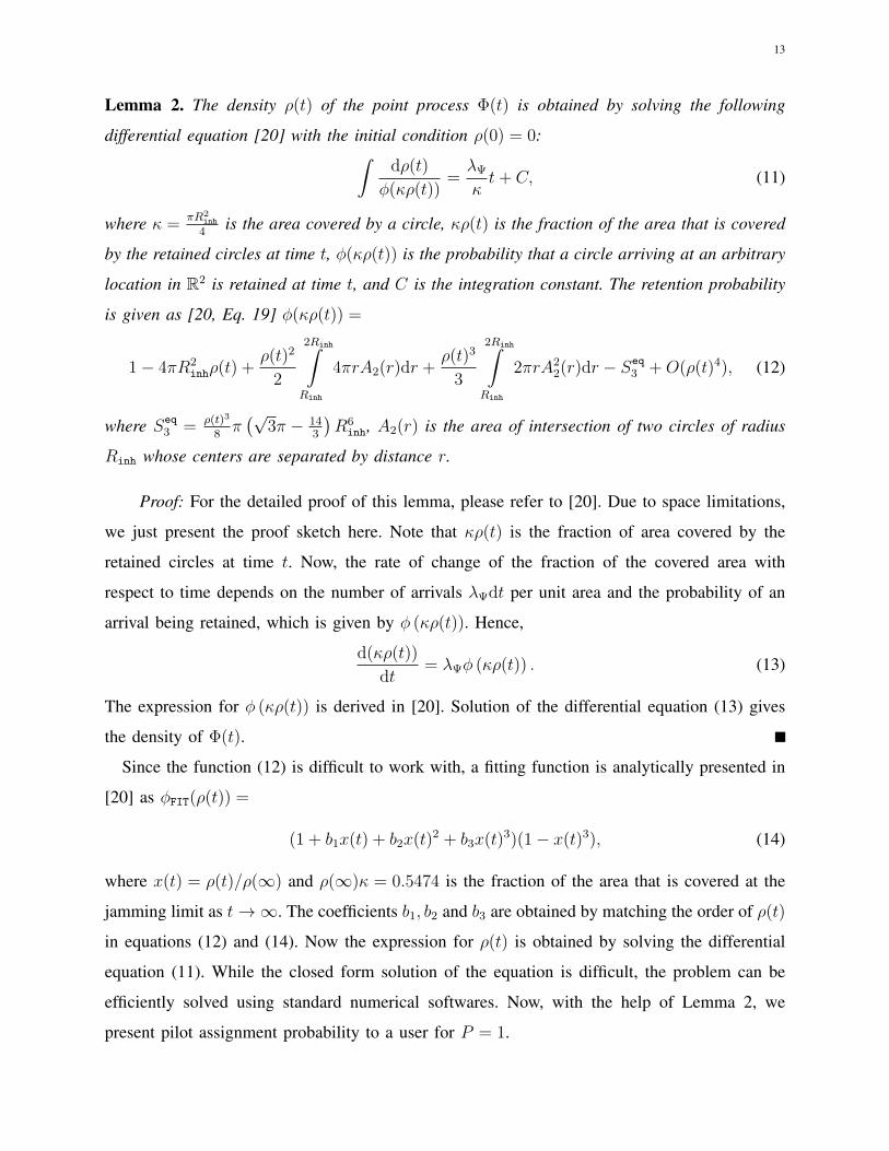
Lemma 2. The density ρ(t) of the point process Φ(t) is obtained by solving the following

differential equation [20] with the initial condition ρ(0) = 0:∫dρ(t)

φ(κρ(t))=λΨ

κt+ C, (11)

where κ = πR2inh

4is the area covered by a circle, κρ(t) is the fraction of the area that is covered

by the retained circles at time t, φ(κρ(t)) is the probability that a circle arriving at an arbitrary

location in R2 is retained at time t, and C is the integration constant. The retention probability

is given as [20, Eq. 19] φ(κρ(t)) =

1− 4πR2inhρ(t) +

ρ(t)2

2

2Rinh∫Rinh

4πrA2(r)dr +ρ(t)3

3

2Rinh∫Rinh

2πrA22(r)dr − Seq

3 +O(ρ(t)4), (12)

where Seq3 = ρ(t)3

8π(√

3π − 143

)R6

inh, A2(r) is the area of intersection of two circles of radius

Rinh whose centers are separated by distance r.

Proof: For the detailed proof of this lemma, please refer to [20]. Due to space limitations,

we just present the proof sketch here. Note that κρ(t) is the fraction of area covered by the

retained circles at time t. Now, the rate of change of the fraction of the covered area with

respect to time depends on the number of arrivals λΨdt per unit area and the probability of an

arrival being retained, which is given by φ (κρ(t)). Hence,

d(κρ(t))

dt= λΨφ (κρ(t)) . (13)

The expression for φ (κρ(t)) is derived in [20]. Solution of the differential equation (13) gives

the density of Φ(t).

Since the function (12) is difficult to work with, a fitting function is analytically presented in

[20] as φFIT(ρ(t)) =

(1 + b1x(t) + b2x(t)2 + b3x(t)3)(1− x(t)3), (14)

where x(t) = ρ(t)/ρ(∞) and ρ(∞)κ = 0.5474 is the fraction of the area that is covered at the

jamming limit as t→∞. The coefficients b1, b2 and b3 are obtained by matching the order of ρ(t)

in equations (12) and (14). Now the expression for ρ(t) is obtained by solving the differential

equation (11). While the closed form solution of the equation is difficult, the problem can be

efficiently solved using standard numerical softwares. Now, with the help of Lemma 2, we

present pilot assignment probability to a user for P = 1.

14

Lemma 3. For a system with P = 1, the probability that the typical user is assigned a pilot is

P[Io = 1] ≈ (1 + πR2sλu)e

−πR2sλu + (1− (1 + πR2

sλu)e−πR2

sλu)(ρ(1)πR2s)E

[N−1u |Nu > 1

],

where ρ(1) is determined using Lemma 2 and E [N−1u |Nu > 1] using (10).

Proof: Since the density of user process Ψu is λu users per unit area, as per the RSA process

definition, we can construct an equivalent space-time process where the arrivals occur at λu users

per unit area per unit time. Now, to obtain the density of Φu, we observe this space-time system

at time t = 1. Hence, the density of Φu is ρ(1). The final expression is obtained by replacing

E[Ns] = πR2sρ(1) in (9).

3) Pilot assignment probability for P ≥ 2: For the general case of P ≥ 2, consider that

Φu1,Φu2, . . . ,ΦuP contain the locations of the users that are assigned the pilots p1,p2, . . . ,pP ,

respectively, by Algorithm 1. Since Algorithm 1 has no preference regarding the pilots, the

densities of Φu1,Φu2, . . . ,ΦuP are the same. Let λΦuo be this density. In order to determine

λΦuo , modifications in Lemma 2 are necessary. To be specific, for (12), the knowledge of virial

coefficients for a mixture of non-interacting hard spheres, and subsequently derivation of Seq3

is necessary [20]. Since the above steps appear extremely difficult for this case, we provide an

approximate yet accurate way to estimate the pilot assignment probability for P ≥ 2.

Input: User locations Ψu, the set of pilots P , inhibition distance Rinh;

Result: Pilot assignment table T ;

Initialization: Ψ′u = Ψu, T = ∅;

for Each pilot pk ∈ P do

for Each user u ∈ Ψ′u do

if No other users in BRinh(u) are using pk then

Assign the pilot: T = T ∪ pk;

Remove u from list of users: Ψ′u = Ψ′

u \ u;

end

end

end

Algorithm 2: The regenerative algorithm for pilot assignment.

First, we present the regenerative pilot assignment algorithm (Algorithm 2) that is essential

for our approximate analysis. Different from Algorithm 1, in Algorithm 2, the pilots are assigned

15

to users sequentially, i.e. for the typical user the second pilot sequence is considered if the first

pilot has already been assigned to a user in its contention domain, the third pilot sequence is

considered if both the first and the second pilots have been used in its contention domain, and

so on. In order to proceed with our analysis, we make the following remark:

Remark 1. The total number of pilot reuses required in BRs(o) to obtain a target pilot assignment

probability is the same for both Algorithms 1 and 2. In other words, the density of users that

are assigned a pilot is the same for both the algorithms.

Let Φu1, Φu2, . . . , ΦuP contain the locations of the users that are assigned pilots p1,p2, . . . ,pP ,

respectively, by Algorithm 2. Let λΦu1, λΦu2

, . . . , λΦuPbe the densities of Φu1, Φu2, . . . , ΦuP ,

respectively. We obtain these densities by sequentially using Lemma 2. First, the density λΦu1

of the users that are assigned the pilot p1 is directly obtained from Lemma 2 where the initial

density of the process is λu. Now, to obtain the density λΦu2of the users that are assigned the

pilot p2, we approximate the initial density of users as λu − λΦu1. Also note that the points

in Ψu \ Φu1 do not form a PPP. However, for simplicity we approximate Ψu \ Φu1 as a PPP.

Similarly, to obtain λΦu3, we approximate Ψu \{Φu1∪ Φu2} as a PPP of density λu−λΦu1

−λΦu2

and use Lemma 2. The same approximation is made to get the rest of the densities. In the next

section, we will demonstrate that these approximations do not compromise the accuracy of our

results. Based on Remark 1, with the knowledge of λΦu1, λΦu2

, . . . , λΦuP, we can obtain

λΦuo =P∑l=1

λΦul/P. (15)

In the next lemma, we present the pilot assignment probability for the general case of P ≥ 1.

Lemma 4. For a system with P ≥ 1, the pilot assignment probability for the typical user is

P[Io = 1] ≈ P[Nu ≤ P ] + P[Nu > P ](PλΦuoπR2s)E[N−1

u |Nu > P ], (16)

where λΦuo is determined from (15) and Lemma 2, E[N−1u |Nu > P ] is determined using (10),

and Nu is Poisson distributed with mean λuπR2s .

Proof: The proof follows on the similar lines as that of Lemma 3.

B. Distributed implementation of the RSA-based pilot allocation scheme

The RSA based pilot allocation scheme can also be implemented in a distributed manner.

Consider the moment when a user uo enters the network. During the initial access phase, the

16

user senses the environment to get an estimate of active pilot transmission in the vicinity. Let

ro ∈ C1×τIA be the received signal obtained through sensing. Note that τIA should span over

multiple coherence time intervals τc to average out the effect of small scale fading. Assuming

synchronization has been established between the network and the user, the received signal

strength on k-th pilot can be estimated as

Pk =1

τIA/τc

τIA/τc∑m=1

ro[(m− 1)τc + 1 : (m− 1)τc + τp]Hpk, (17)

where τp is the duration of the pilot sequence. Once the received signal powers on all the pilots

are calculated, they are compared with a threshold power Pinh, which is a function of Rinh. A

pilot is randomly selected from the set of candidate pilots {pk : Pk ≤ Pinh}. If this set is empty,

then the user is not assigned a pilot. Algorithm 3 presents the above-mentioned procedure.

Input: Power threshold Pinh, Received signal ro;Result: Pilot for user uo;Initialization: Candidate set of pilots Pc = ∅ ;for Each pilot pk ∈ P do

Obtain Pk using (17) ;if Pk ≤ Pinh thenPc = Pc ∪ pk ;

endendif Pc 6= ∅ then

Select a pilot randomly from Pc.

end

Algorithm 3: The algorithm for an arriving user to select a pilot during initial access phase.

IV. MAX-MIN DISTANCE-BASED PILOT ALLOCATION SCHEME

While the proposed RSA-based scheme is a computationally efficient scheme with possible

distributed implementation, a natural question is how good is the quality of the solution. In this

section, we propose an algorithm that has the objective of maximizing the minimum distance

between the set of co-pilot users similar to the RSA-based scheme. However, in contrast to

the RSA scheme that can be implemented in a distributed manner, this algorithm can only be

implemented in a centralized way and does not have the scalability property of the RSA-based

scheme.

To have a meaningful problem formulation, we restrict our attention to a finite spatial ob-

servation window W ⊂ R2. Let the set of users in this observation window be given as

S = {u1,u2, . . . ,uNu}. Our objective is to partition S into P sets S1,S2, . . . ,SP such that

17

the minimum distance between any two users in a partition is maximized. For a user un,

the binary variable ynk = 1 if the user belongs to Sk and 0 otherwise. We define the metric

dmin(Sk) := min{‖ui − uj‖ : ui 6= uj, yik = yjk = 1} as the minimum distance between two

elements in Sk. The problem of maximizing the minimum distance between users belonging to

the same set can be written as

max{ynk}

mink=1,...,P

dmin(Sk) (18a)

s.t.P∑k=1

ynk = 1, ∀n = 1, 2, . . . , Nu, (18b)

Nu∑n=1

ynk > 1, ∀k = 1, 2, . . . , P, (18c)

ynk ∈ {0, 1}, ∀n,∀k, (18d)

where (18b) ensures that each point belongs to exactly one partition, (18c) ensures that each

partition has more than two points, (18d) imposes the integrality constraint. Note that (18c) can

be modified to ensure more balanced partitioning. For example, if we need each partition to

have more than x ≤ Nu/P users then we can set the constraint as∑N

n=1 ynk > x, ∀k. This

problem can be reformulated as

maxt,ynk

t (19a)

s.t. ‖ui − uj‖ > tyikyjk ui ∈ S,uj ∈ S, i 6= j, k = 1, 2, . . . P, (19b)

P∑k=1

ynk = 1, ∀n = 1, 2, . . . , Nu, (19c)

Nu∑n=1

ynk > 1, ∀k = 1, 2, . . . , P, (19d)

ynk ∈ {0, 1}, ∀n,∀k, (19e)

where (19b) ensures that two points belonging to the same partition are separated by distance t

and rest of the constraints are the same as the previous formulation. The aforementioned problem

can be solved in two steps. In the first step, a bisection search is used to improve the objective

function, and in the second step for a given t, a feasibility problem is solved. The optimization

routine to solve the problem is presented in Algorithm 4.

Both the algorithms mentioned so far do not take into account the distances among the users

and the RRHs. As a consequence, two users that are separated by a reasonable distance, but

18

1: Initialization: Set the values of tmin and tmax that define the solution space for the bisection search. Select a

tolerance parameter ε.

2: Set t = (tmin + tmax)/2. Solve the following feasibility problem:

K∑k=1

ynk = 1 ∀n = 1, 2, . . . , Nu (20a)

Nu∑n=1

ynk > 1 ∀k = 1, 2, . . . , P (20b)

yik + yjk ≤ 1 ∀‖ui − uj‖ < t, (20c)

ynk ∈ {0, 1} ∀n, ∀k. (20d)

3: if (20) is feasible then

4: Set tmin = t.

5: else

6: Set tmax = t.

7: end if

8: Repeat the above steps until if |tmax − tmin| < ε.

Algorithm 4: Solving the max-min distance partitioning problem

have a common set of dominant RRHs may be assigned the same pilot. In such a scenario, both

the users will experience performance degradation. This scenario is more likely to occur when

the density of RRHs is low. In order to overcome this performance degradation, in the following

section we propose a centralized RRH location aware pilot allocation algorithm.

V. RRH LOCATION AWARE PILOT ALLOCATION SCHEME

In this section, we present a heuristic algorithm to solve the original pilot allocation problem

(8) presented in Sec. III. Despite a few useful constraints that we introduce to the problem to limit

the size of the feasible solution space, the complexity of the problem still remains high. Hence,

the practical utility of the algorithm is somewhat questionable in a large network (hundreds of

users), but it provides an excellent opportunity for benchmarking any pilot allocation algorithms

for a smaller network with tens of users. Further, we use this scheme to benchmark the RSA-

based and max-min distance-based algorithms proposed in the previous sections.

In order to reduce the space of good quality feasible solutions, we first use a clustering

algorithm to group the users that have a similar path-loss with respect to the set of RRHs. Once

19

the clusters of users are obtained, we use BnP algorithm to solve the sum SE maximization

problem with the additional constraint that users in the same cluster cannot be assigned the

same pilot. In the following two subsections, we discuss the clustering algorithm followed by a

brief overview of the BnP algorithm with application to the problem at hand.

A. RRH location-aware user clustering based on spectral graph theory

We use a spectral graph theory-based algorithm to cluster users with similar propagation char-

acteristics. Before proceeding further, we present a few graph theoretic notations and definitions

that are required for a rigorous exposition.

1) Graph definitions: Consider the weighted undirected graph G = (V , E ,W), where V =

{v1, v2, . . . , vn} is known as the vertex set, E = {eij}i,j=1,...,n is the edge set that contains

the edges connecting these vertices, and W = {wij}i,j=1,...,n is a set of non-negative weights

assigned to each edge. If two vertices i, j are connected then eij = 1 and wij > 0. Otherwise,

eij = wij = 0. The adjacency matrix of the graph G is denoted by A ∈ {0, 1}n×n and defined

as A(i, j) = eij. Further, the weighted adjacency matrix is given as W ∈ Rn×n and defined as

W (i, j) = wij . The degree matrix of a weighted graph G, denoted by D ∈ Rn×n, is a diagonal

matrix whose i-th diagonal element is given as D(i, i) =∑n

j=1 wij. The Laplacian matrix of the

graph G is defined as L = D −W . The K-cut of the graph G is defined as

cut(V1,V2, . . . ,VK) =1

2

K∑i=1

∑vl∈Vi,vm∈VC

i

wlm,

where Vi is the i-th partition of V . Further, ∪Ki=1Vi = V and Vi ∩ Vj = ∅ for i 6= j. The volume

of a partition Vi is defined as

Vol(Vi) =∑vj∈Vi

D(j, j).

The graph G is bipartite, if the vertex set can be partitioned into two sets X ,Y ⊂ V such that

the edges in E have one end point in X and another end point in Y . Further, the graph G is a

connected graph, if there is at least one path between any two vertices. Next, we formulate the

problem of clustering users with similar propagation characteristic, namely the path-loss.

2) Graph theoretic formulation of the clustering problem: We consider a weighted bipartite

graph where the vertices are the sets of users Ψu = Ψu ∩W and RRHs Φr = Φr ∩W over the

finite spatial observation window W . An edge exists between each RRH and each user, but no

20

edge exists among the RRHs or the users. The weight of an edge is the path-loss between a user

and a RRH. In terms of the notations introduced earlier, V = Ψu ∪ Φr, E = {emk = 1 : uk ∈

Ψu, rm ∈ Φu}, and W = {wmk = βmk : uk ∈ Ψu, rm ∈ Φr}. As mentioned earlier, |Ψu| = Nu

and |Φ| = Nr. The degree matrix is given as

D =

Du 0Nu×Nr

0TNu×NrDr

∈ R(Nu+Nr)×(Nu+Nr),

where Du ∈ RNu×Nu is the degree matrix for the users and Dr ∈ RNr×Nr is the degree matrix

for the RRHs. Further, the weighted adjacency matrix for the considered bipartite graph is

W =

0Nu×Nu WUR

W TUR 0Nr×Nr

∈ R(Nu+Nr)×(Nu+Nr),

where the rows of WUR ∈ RNu×Nr represent the weights associated with a user with respect

to all the RRHs. The problem of user clustering is based on the idea of partitioning the graph

into desired number of groups such that edges across the groups have the lowest weights. In

the current case, the output of the partitioning algorithm should be the clusters of users along

with corresponding set of dominant RRHs such that the sum of edge weights between a set of

clustered users and corresponding set of non-dominant RRHs should be minimum. The problem

can be formally stated as a min-cut problem presented below:

minimizeV1,V2,...,VK

cut(V1,V2, . . . ,VK) = minimizeV1,V2,...,VK

K∑k=1

1

2

∑vl∈Vk,vm∈VC

k

wlm

subject toK⋃k=1

Vk = V ,K⋂k=1

Vk = ∅, (21)

where Vk = Ψk∪Φk contains the nodes (both users and RRHs) corresponding to the k-th cluster.

Different algorithms exist to solve the above min-cut problem. However, one major drawback

of these algorithms is that they partition the vertices into unequal groups. To circumvent this

problem, normalized ratio cut (Ncut) is considered as the objective instead of the cut presented

in (21) [21]. Hence, the modified optimization problem can be written as

minimizeV1,V2,...,VK

Ncut(V1,V2, . . . ,VK) = minimizeV1,V2,...,VK

K∑k=1

1

2

∑vl∈Vk,vm∈VC

kwlm

Vol(Vk),

subject toK⋃k=1

Vk = V ,K⋂k=1

Vk = ∅. (22)

The aforementioned problem is NP-hard in nature. However, an efficient approximate solution

can be obtained by relaxing the above problem that is presented next.

21

3) Spectral graph theory to solve the Ncut problem: The general idea of the algorithm is

composed of two steps. In the first step, user locations are transformed into a space that captures

the propagation characteristics between the set of users and the set of RRHs. In the second step,

user clustering is performed by K-means algorithm to the transformed user and RRH locations.

For the i-th cluster Vi, let us define the vector fi ∈ RNt×1 whose j-th element is given as

fij =

1√

Vol(Vi), if vj ∈ Vi

0, if vj ∈ VCi ,

where Nt = Nu + Nr. Note that based on the definition of the degree matrix, fTi Dfi = 1.

Further, in case of the Laplacian matrix of the graph, fTi Lfi = cut(Vi,VCi )/Vol(Vi). Verifying

these statements is straightforward and we refer the reader to [21] (and the references therein)

for further insights on the graph Laplacian.

Let the matrix F = [f1, f2, . . . , fK ]. Now, the optimization problem in (22), can be written as

minimizeF

Tr(F TLF

), subject to F TDF = IK . (23)

The optimal solution for the columns of F should only take discrete binary values. However,

due to the NP-hard nature of the problem, a relaxed version of the above problem is solved,

which is given as

minimizeF∈RNt×K

Tr(F TLF

), subject to F TDF = IK . (24)

Substituting Z = D1/2F , we get

minimizeZ∈RNt×K

Tr(ZTD−1/2LD−1/2Z

), subject to ZTZ = IK . (25)

Note that the above problem is convex and can be solved by reducing it to an unconstrained

optimization problem using Lagrange multiplier [22]. In the following lemma, the solution to

the (25) is presented.

Lemma 5. The solution to (25) consists of K eigenvectors corresponding to the K smallest

non-zero eigenvalues of D−1/2LD−1/2.

Proof: The Lagrangian of (25) is given as [22]

L(Z,Σ) = Tr(ZTD−1/2LD−1/2Z

)+ Tr

(ΣT (ZTZ − IK)

).

22

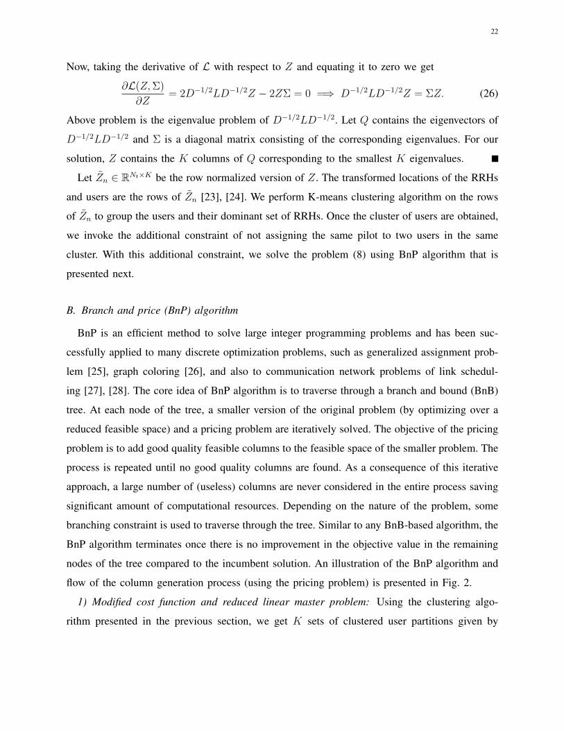
Now, taking the derivative of L with respect to Z and equating it to zero we get

∂L(Z,Σ)

∂Z= 2D−1/2LD−1/2Z − 2ZΣ = 0 =⇒ D−1/2LD−1/2Z = ΣZ. (26)

Above problem is the eigenvalue problem of D−1/2LD−1/2. Let Q contains the eigenvectors of

D−1/2LD−1/2 and Σ is a diagonal matrix consisting of the corresponding eigenvalues. For our

solution, Z contains the K columns of Q corresponding to the smallest K eigenvalues.

Let Zn ∈ RNt×K be the row normalized version of Z. The transformed locations of the RRHs

and users are the rows of Zn [23], [24]. We perform K-means clustering algorithm on the rows

of Zn to group the users and their dominant set of RRHs. Once the cluster of users are obtained,

we invoke the additional constraint of not assigning the same pilot to two users in the same

cluster. With this additional constraint, we solve the problem (8) using BnP algorithm that is

presented next.

B. Branch and price (BnP) algorithm

BnP is an efficient method to solve large integer programming problems and has been suc-

cessfully applied to many discrete optimization problems, such as generalized assignment prob-

lem [25], graph coloring [26], and also to communication network problems of link schedul-

ing [27], [28]. The core idea of BnP algorithm is to traverse through a branch and bound (BnB)

tree. At each node of the tree, a smaller version of the original problem (by optimizing over a

reduced feasible space) and a pricing problem are iteratively solved. The objective of the pricing

problem is to add good quality feasible columns to the feasible space of the smaller problem. The

process is repeated until no good quality columns are found. As a consequence of this iterative

approach, a large number of (useless) columns are never considered in the entire process saving

significant amount of computational resources. Depending on the nature of the problem, some

branching constraint is used to traverse through the tree. Similar to any BnB-based algorithm, the

BnP algorithm terminates once there is no improvement in the objective value in the remaining

nodes of the tree compared to the incumbent solution. An illustration of the BnP algorithm and

flow of the column generation process (using the pricing problem) is presented in Fig. 2.

1) Modified cost function and reduced linear master problem: Using the clustering algo-

rithm presented in the previous section, we get K sets of clustered user partitions given by

23

Obtain the RMP form MP

Positive reduced cost columns

found

Current RLMP solution is optimal

Yes

No

Ad

d c

olu

mn(

s) t

o R

LM

P

Solve the RLMP

Solve the pricing problem

Fig. 2: The branch and bound tree (left). The column generation algorithm flow chart (right).

{V1,V2, . . . ,VK}. To ensure that users in the same cluster are not assigned the same pilot, we

modify the cost function (7) as

c(xj) =

∑

ui∈Ajlog2 (1 + Γij) , if Γij ≥ Γmin ∀ui ∈ Aj

−M, if Γij < Γmin for any ui ∈ Aj

−M, if |Vk ∩ Aj| > 1 for any k = 1, 2, . . . K,

(27)

where the last row ensures that the columns that have users from the same cluster are (almost)

never considered as good columns in the pricing problem. Based on the above definition of the

cost function, to make sure that the original problem remains feasible, number of users in a

cluster should be less than the number of pilots. Hence, we choose K = max{P,Nu/P}. We

call (8) with the modified cost function definition as the master problem (MP). Further, we refer

to the problem with relaxed integer constraint (8d) of the MP as linear master problem (LMP),

which is expressed as

maxΛ

|A|∑s=1

c(xs)λs (28a)

s.t. AΛ = 1 (28b)

‖Λ‖1 = P (28c)

Λ ∈ [0, 1]|A|. (28d)

24

As mentioned earlier, at each node of the BnB tree, we solve the problem with a subset of

all potential columns in A, and gradually keep adding good columns determined by the pricing

algorithm. We define the set H ⊂ A and the corresponding matrix as H , which contains a few

of the columns of A. We refer to this problem as the reduced linear master problem (RLMP),

which is given as

maxΛ

|H|∑s=1

c(xs)λs (29a)

s.t. HΛ = 1 (29b)

‖Λ‖1 = P (29c)

Λ ∈ [0, 1]|H|. (29d)

Let Π = [π1, π2, . . . , πNu ] be the set of dual variables that correspond to the constraint (29c)

and β be the dual variable for the constraint (29d). Note that the optimal set of dual variable

for LMP is also the optimal set of dual variables for RLMP.

2) Pricing problem: At each node of the BnB tree, the RLMP is solved to optimality using any

linear programming method, such as the simplex, and the corresponding dual variables are used

to obtain new columns that can improve the objective of RLMP by solving a pricing problem.

The idea behind the pricing problem can be better understood from the Lagrange function of

LMP, which is given as

L(Π, β,Λ) =

|A|∑s=1

c(xs)λs − ΠT (AΛ− 1)− β(‖Λ‖1 − P ). (30)

Note that if a given set of solutions Λ∗ is optimal for the LMP, then the first derivative of L

with respect to each variable is zero. On the other hand, for a given set of dual variables, if we

can improve the value of L by increasing the value of λj , then it must be the case that

∂L(Π, β,Λ)

∂λj= c(xj)− ΠTxj − β > 0. (31)

The quantity c(xj) − ΠTxj − β is known as the positive reduced cost of the column xj . This

provides us a direct way to add new columns to an RLMP that can improve its objective function

value. To be specific, for a given set of dual variables (Π, β) corresponding to a RLMP, the pricing

problem is given as

arg maxx∈A

c(x)− ΠTx− β, (32)

25

and the optimal column is added to the RLMP, thus obtaining an augmented matrix H . The RLMP

is solved again using H and the new set of dual variables are used in the pricing problem to get

better columns. The procedure is repeated until there is no column in A with positive reduced

cost, i.e. c(x)−ΠTx− β ≤ 0 for all the columns in A \ H. The flow of the column generation

process is given in Fig. 2 (right). Note that even with the linear relaxation (32) is a non-convex

non-linear problem. Hence, solving it to optimality in polynomial time is not possible. However,

meta-heuristic algorithms such as the genetic algorithm, or tabu search, can be used to get

efficient solutions. In this work, we focus on solving (32) with exhaustive enumeration over

the set of feasible columns. This process is significantly more efficient compared to solving the

original problem through exhaustive enumeration.

Note that the optimal solution of the RLMP, i.e. Λ∗, is not guaranteed to be an integral solution.

The following branching rule in the BnB tree ensures that the optimal solution to the RLMP is

an integer vector, thereby making Λ∗ an optimal solution to the original RMP problem that has

the integrality constraint.

3) Branching rule: The objective of the branching rule is to progressively introduce branching

constraints such that eventually the solution to the RLMP becomes integral [25]. The branching

rule is derived from a relatively well-known result in the linear programming literature that is

stated in the following lemma.

Lemma 6. Consider the linear maximization problem {max cTx : Ax = 1,x > 0}. If A is a

totally balanced matrix, then the optimal solution x∗ is integer valued.

For the proof along with detailed discussion of the result stated in the lemma, please refer

to [29]. After solving the RLMP and pricing problem to (near) optimality, the objective is to

introduce the branching constraints such that the augmented matrix of the RLMP H eventually

becomes a totally balanced matrix as we traverse through the BnB tree. As mentioned in [25],

this can be achieved by the constraints hpk = hrk on one branch and hpk = hrk = 0 or hpk 6= hrk

on the other branch, where hpk is the element corresponding to the p-th row and k-th column of

H . The branching constraint implicitly ensures that on one branch two users belong to the same

column, while on the other branch the users belong to two different columns. These branching

constraints are introduced in the RLMP and also used in the column generation process.

4) Node pruning and termination criterion for the BnB tree: The backbone of the BnP

algorithm is the BnB algorithm. To harvest full benefits of the BnB tree, it is essential to

26

introduce efficient node pruning criteria so that unnecessary nodes are never visited. Let z∗MP,

z∗LMP are the optimal values of the MP and LMP, respectively. Further, z∗LMP ≤ zRLMP +Pc, where

c is the maximum positive reduced cost of columns for a given RLMP. When the RLMP along

with pricing problem is solved to optimality, z∗LMP = z∗RLMP, since there exists no column that

can improve the value of z∗RLMP. Let zinc be the incumbent solution, which is always integral in

nature. If at a node of BnB tree, we have z∗RLMP < zinc, subsequent nodes in the branch will not

provide any better solution. Hence, the pruning occurs at this node of the branch, i.e., subsequent

nodes on the same branch are not explored and the nodes on the other branches are explored.

Once no nodes with z∗RLMP > zinc are found, zinc is the optimal solution.

VI. RESULTS

In this section, through Monte Carlo simulations, we validate the theoretical analysis on pilot

assignment probability and assess the performance of the RSA-inspired pilot allocation compared

to other schemes presented in this work. The simulations environment for each scenario is

presented in the specific subsection.

A. Performance of the RSA-based pilot allocation scheme

In this case, for the simulations, we consider a network of radius 1500 m. In order to avoid edge

effects, points within 600 m are considered. The average user spectral efficiency is reported for the

typical user located at the center. We use the following non-line-of-sight path-loss function [30]:

l(d) =161.04− 7.1 log10(W ) + 7.5 log10(h)− [24.37− 3.7(h/hAP)2] log10(hAP)

+ [43.42− 3.1 log10(hAP)][log10(d)− 3] + 20 log10(fc)− (3.2[log10(11.75hAT)2]− 4.97),

where W = 20, hAP = 40, hAT = 1.5, h = 5, fc = 0.45 GHz.

In Fig. 3 (left), the co-pilot user density as a function of number of pilots is presented. As

expected, the co-pilot user density decreases with increasing number of pilots. In Fig. 3 (center),

we present the pilot assignment probability as a function of the number of pilots. This result

is useful in determining the number of pilots that is required to achieve a certain assignment

probability. Finally, in Fig. 3 (right), we present the average user SE as a function of Rinh. To

generate this result, we set the uplink pilot SNR ρp = 80 dB, length of pilot sequence τp = P = 16.

We observe that with increasing λu, the optimal Rinh that maximizes user SE becomes smaller.

Further, there exists a range of Rinh that provides higher user SE compared to the random pilot

assignment scheme [6]. However, this range shrinks as λu increases.

27

Number of Pilots

0 10 20 30 40 50 60

Co

-Pil

ot

Use

r D

ensi

ty

0

0.05

0.1

0.15

Rinh = {100, 150, 200}mλu = 10−4users/m2

Rinh = 100mλu = {1, 2, 3}10−4

Number of Pilots0 10 20 30 40 50 60

Probabilityofpilotassignment

0

0.2

0.4

0.6

0.8

1

λu = 3× 10−4

Rinh = 300

λu = 3× 10−4

Rinh = 200

Rinh

0 100 200 300 400 500 600

Av

erag

e U

ser

SE

0

5

10

15

λu = 5× 10−4,

λr = 5× 10−4

λu = 5× 10−5,

λr = 5× 10−4

λu = 10−4,

λr = 5× 10−4

Fig. 3: The co-pilot user density as a function of P (left), Probability of pilot assignment as a function P (center), and Average

user SE as a function of Rinh (right). In the first two figure, markers and solid lines represent simulations and theoretical results,

respectively.

B. Performance comparison of RSA-based scheme to the max-min distance-based scheme

In this subsection, we compare the performance of the RSA scheme to the max-min distance-

based scheme. Further, we also provide the relative performance between RSA and the following

two existing schemes in the literature: iterative K-means-based algorithm [14] and the random

pilot allocation algorithm [6]. In the case of the RSA-based scheme, for a given λr and λu, the

Rinh that maximizes the average user SE is selected. The simulation environment remains the

same as that of the previous subsection. In Fig. 4, we present the ratio of the average user SEs

of different schemes with respect to the average user SE of the RSA scheme. From the results,

we conclude that the system performance is primarily affected by (i) the average number of

users per pilot and (ii) RRH density. When the average number of users per pilot is relatively

low, the RSA scheme marginally outperforms the max-min as well as the iterative K-means

algorithms, especially at the low RRH density. On the other hand, with a relatively high average

number of users per pilot, the max-min scheme performs marginally better compared to both the

RSA and iterative K-means algorithm. In the case of the RSA, this slightly inferior performance

can be attributed to the reduced pilot assignment probability in a dense environment. All the

three schemes provide significant average user SE improvement over the random pilot allocation

scheme.

C. Performance comparison of the RSA-based scheme to the BnP scheme

Since the RRH location-aware heuristic scheme based on BnP algorithm exhibits significant

computational complexity for a large system (hundreds of users), we compare the performance

for a relatively small system with 48 users uniformly distributed over a circular area of radius

28

RRH density (λr)10

-610

-510

-4

Ratio

ofaverageuserSEs

0.75

0.8

0.85

0.9

0.95

1

1.05

RSA

K-Means

Max-Min

Random

RRH density (λr)10

-610

-510

-4

Ratio

ofaverag

euserSEs

0.7

0.75

0.8

0.85

0.9

0.95

1

1.05

RSA

K-Means

Max-Min

Random

RRH density (λr)10

-610

-510

-4

Ratio

ofaverag

euserSEs

0.75

0.8

0.85

0.9

0.95

1

1.05

RSA

K-Means

Max-Min

Random

Fig. 4: The ratio of average user SEs of different schemes with respect to the RSA-based scheme for different system

configurations: (left) λu = 10−5, P = 16; (center) λu = 10−4, P = 16; (right) λu = 10−5, P = 8.

400 m. Further, these users are simultaneously served by Nr RRHs distributed uniformly over

the same area. The path-loss function remains the same as given in the previous subsection. In

Fig. 5, we present the cumulative distribution function (CDF) of the ratio of sum user SEs for

the RSA to BnP scheme. As observed from Fig. 5 (left), the performance of the RSA scheme

improves with the increasing number of RRHs in the system. However, the effect of number of

pilots on the relative performance of RSA compared to the BnP scheme is negligible as evident

from Fig. 5 (right), where RSA gives similar performance for different number of pilots.

Ratio of Sum SE of RSA to BNP

0.7 0.75 0.8 0.85 0.9 0.95 1

CDF

0

0.2

0.4

0.6

0.8

1

Nr = 5, 10, 15, 20, 30

Ratio of Sum SE RSA to BNP

0.8 0.85 0.9 0.95 1

CDF

0

0.2

0.4

0.6

0.8

1

P = 10

P = 12

P = 8

Fig. 5: The CDF of the ratio of sum user SE of RSA to BnP scheme for different system configuration: (left) Nu = 48, P = 10;

(right) Nu = 48, Nr = 10.

VII. CONCLUSION

In this work, we proposed a pilot assignment algorithm to mitigate the effect of pilot con-

tamination for cell-free mMIMO systems. Our algorithm is inspired by the RSA process, which

has been used to study the adsorptions of hard particles on a surface across different scientific

29

disciplines. Using the well-developed analytical tools for the RSA process, we presented an

accurate theoretical expression for average pilot assignment probability for the typical user in

the network. Further, the performance of the proposed algorithm was compared to two centralized

pilot allocation schemes. With respect to the first centralized scheme, which partitions the users

in the network such that the minimum distance among the sets of co-pilot users is maximized, the

RSA-based scheme provides competitive average user SE performance. The second centralized

pilot allocation scheme, which is based on the BnP algorithm, provides a near-optimal solution

in terms of sum user SE for a relatively small system with tens of users. The performance of

the RSA-based scheme is appreciable with respect to the near-optimal BnP scheme. Owing to

its competitive performance and scalable distributed implementation, the RSA-based scheme is

an attractive algorithm for pilot allocation in a pilot contamination limited cell-free mMIMO

network. Although technically challenging, a promising future direction of this work is to

investigate a more efficient solution for the pricing problem used in the column generation

process so that the BnP-based scheme can be used to benchmark the performance of even larger

systems with hundreds of users.

REFERENCES

[1] P. Parida and H. S. Dhillon, “Random sequential adsorption-based pilot assignment for distributed massive MIMO systems,”

in Proc., IEEE Globecom, 2019, pp. 1–6.

[2] R. Irmer, H. Droste, P. Marsch, M. Grieger, G. Fettweis, S. Brueck, H. Mayer, L. Thiele, and V. Jungnickel, “Coordinated

multipoint: Concepts, performance, and field trial results,” IEEE Commun. Magazine, vol. 49, no. 2, pp. 102–111, February

2011.

[3] A. Checko, H. L. Christiansen, Y. Yan, L. Scolari, G. Kardaras, M. S. Berger, and L. Dittmann, “Cloud RAN for mobile

networks–a technology overview,” IEEE Commun. Surveys and Tutorials, vol. 17, no. 1, pp. 405–426, Firstquarter 2015.

[4] O. Y. Bursalioglu, G. Caire, R. K. Mungara, H. C. Papadopoulos, and C. Wang, “Fog massive MIMO: A user-centric

seamless hot-spot architecture,” IEEE Trans. on Wireless Commun., vol. 18, no. 1, pp. 559–574, Jan 2019.

[5] E. Nayebi, A. Ashikhmin, T. L. Marzetta, H. Yang, and B. D. Rao, “Precoding and power optimization in cell-free massive

MIMO systems,” IEEE Trans. on Wireless Commun., vol. 16, no. 7, pp. 4445–4459, July 2017.

[6] H. Q. Ngo, A. Ashikhmin, H. Yang, E. G. Larsson, and T. L. Marzetta, “Cell-free massive MIMO versus small cells,”

IEEE Trans. on Wireless Commun., vol. 16, no. 3, pp. 1834–1850, March 2017.

[7] T. L. Marzetta, “Noncooperative cellular wireless with unlimited numbers of base station antennas,” IEEE Trans. on

Wireless Commun., vol. 9, no. 11, pp. 3590–3600, November 2010.

[8] E. Bjornson, J. Hoydis, and L. Sanguinetti, “Massive MIMO has unlimited capacity,” IEEE Trans. on Wireless Commun.,

vol. 17, no. 1, pp. 574–590, Jan 2018.

[9] O. Y. Bursalioglu, C. Wang, H. Papadopoulos, and G. Caire, “RRH based massive MIMO with “on the fly” pilot

contamination control,” in Proc., IEEE Intl. Conf. on Commun. (ICC), May 2016, pp. 1–7.

30

[10] M. Attarifar, A. Abbasfar, and A. Lozano, “Random vs structured pilot assignment in cell-free massive MIMO wireless

networks,” in Proc., IEEE Intl. Conf. on Commun. Workshops (ICC Workshops), May 2018, pp. 1–6.

[11] J. Zhang, X. Yuan, and Y. J. Zhang, “Locally orthogonal training design for cloud-RANs based on graph coloring,” IEEE

Trans. on Wireless Commun., vol. 16, no. 10, pp. 6426–6437, Oct 2017.

[12] W. Hmida, V. Meghdadi, A. Bouallegue, and J. P. Cances, “Graph coloring based pilot reuse among interfering users in

cell-free massive MIMO,” in Proc., IEEE Intl. Conf. on Commun. (ICC), May 2020.

[13] W. Zeng, Y. He, B. Li, and S. Wang, “Pilot assignment for cell-free massive MIMO systems using a weighted graphic

framework,” IEEE Trans. on Veh. Technology, pp. 1–1, 2021.

[14] R. Sabbagh, H. Zhu, and J. Wang, “Pilot allocation and sum-rate analysis in distributed massive MIMO systems,” in Proc.,

IEEE Veh. Technology Conf. (VTC), Sep. 2017, pp. 1–5.

[15] H. Liu, J. Zhang, X. Zhang, A. Kurniawan, T. Juhana, and B. Ai, “Tabu-search-based pilot assignment for cell-free massive

MIMO systems,” IEEE Trans. on Veh. Technology, vol. 69, no. 2, pp. 2286–2290, 2020.

[16] S. Buzzi, C. D’Andrea, M. Fresia, Y.-P. Zhang, and S. Feng, “Pilot assignment in cell-free massive MIMO based on the

Hungarian algorithm,” IEEE Wireless Communications Letters, 2020.

[17] H. Q. Nguyen, F. Baccelli, and D. Kofman, “A stochastic geometry analysis of dense IEEE 802.11 networks,” in Proc.,

IEEE Int. Conf. on Comput. Commun., May 2007, pp. 1199–1207.

[18] A. Busson and G. Chelius, “Capacity and interference modeling of CSMA/CA networks using SSI point processes,”

Telecommun. Syst., vol. 57, no. 1, pp. 25–39, Sep. 2014.

[19] J. Talbot, G. Tarjus, P. V. Tassel, and P. Viot, “From car parking to protein adsorption: an overview of sequential adsorption

processes,” Colloids and Surfaces A: Physicochemical and Engineering Aspects, vol. 165, no. 1, pp. 287 – 324, 2000.

[20] P. Schaaf and J. Talbot, “Surface exclusion effects in adsorption processes,” J. Chem. Phys., vol. 91, no. 7, pp. 4401–4409,

1989.

[21] U. Von Luxburg, “A tutorial on spectral clustering,” Statistics and computing, vol. 17, no. 4, pp. 395–416, 2007.

[22] S. Boyd and L. Vandenberghe, Convex optimization. Cambridge university press, 2004.

[23] A. Ng, M. Jordan, and Y. Weiss, “On spectral clustering: Analysis and an algorithm,” Adv. Neural Inf. Process. Syst.,

vol. 14, pp. 849–856, 2001.

[24] I. S. Dhillon, “Co-clustering documents and words using bipartite spectral graph partitioning,” in Proceedings of ACM

SIGKDD Int. Con. on Knowledge discovery and Data mining, 2001, pp. 269–274.

[25] C. Barnhart, E. L. Johnson, G. L. Nemhauser, M. W. Savelsbergh, and P. H. Vance, “Branch-and-price: Column generation

for solving huge integer programs,” Operations research, vol. 46, no. 3, pp. 316–329, 1998.

[26] A. Mehrotra and M. A. Trick, “A column generation approach for graph coloring,” Informs Journal on Computing, vol. 8,

no. 4, pp. 344–354, 1996.

[27] L. Fu, S. C. Liew, and J. Huang, “Fast algorithms for joint power control and scheduling in wireless networks,” IEEE

Trans. on Wireless Commun., vol. 9, no. 3, pp. 1186–1197, 2010.

[28] M. Johansson and L. Xiao, “Cross-layer optimization of wireless networks using nonlinear column generation,” IEEE

Trans. on Wireless Commun., vol. 5, no. 2, pp. 435–445, 2006.

[29] A. J. Hoffman, A. W. J. Kolen, and M. Sakarovitch, “Totally-balanced and greedy matrices,” in Selected Papers Of Alan

J Hoffman: With Commentary. World Scientific, 2003, pp. 328–337.

[30] “Guidelines for evaluation of radio interface technologies for IMT-Advanced,” Report ITU-R, vol. M.2135-1, Dec 2009.