Performance Evaluation of The VSC-Interfaced Distributed ... · Performance Evaluation of The VSC-Interfaced Distributed Resource Models Gorken Gumustekin Master of Applied Science

Performance Evaluation of The VSC-Interfaced Distributed ResourceModels

by

Gorken Gumustekin

A thesis submitted in conformity with the requirementsfor the degree of Master of Applied Science

Graduate Department of Electrical and Computer EngineeringUniversity of Toronto

c© Copyright 2016 by Gorken Gumustekin

Abstract

Performance Evaluation of The VSC-Interfaced Distributed Resource Models

Gorken Gumustekin

Master of Applied Science

Graduate Department of Electrical and Computer Engineering

University of Toronto

2016

The voltage-sourced converter (VSC) is the mostly used converter configuration for grid integration

of distributed resources, i.e., generation and storage units. For such applications, the VSC is conven-

tionally controlled by means of an inner-current controller that operates the VSC based on the desired

VSC current to meet the system operational requirements. In compliance with the principles of the

inner-current controller, the current-injection model has been widely used to represent the VSC impact

studied of the grid-integrated DG.

This thesis investigates the validity of the VSC current-injection model under the unbalanced condi-

tions of feeder and low short-circuit ratios. The objective is establish the degree of accuracy of impact

studies based on the current-injection model.

A test system has been selected and the steady-state and transient-response of a 1.5 MW VSC based

detailed switched-model and the current-injection model under various unbalanced and the system short-

circuit capacity have been investigated and compared.

ii

Acknowledgements

First and foremost, I would like to give sincere thanks to my supervisor Prof. Reza Iravani for his valu-

able time, continuous support and guidance throughout my masters degree education. I cannot thank

him fairly enough for his encouragement and kindly assistance.

I would also like to thank Dr. Milan Graovac and Mr. Xiaolin Wang for their many hours of weekly

discussion which has helped my understanding of the concepts in this thesis. Their endless help is a

critical factor for this thesis.

Moreover, I am thankful to my country for supporting me during Master.

I would like to extend my deepest wholehearted thanks to my parents for their faithful devotions for me.

iii

Contents

1 Introduction 1

1.1 Problem Statement . . . . . . . . . . . . . . . . . . . . . . . . . . . . . . . . . . . . . . . . 1

1.2 Thesis Objectives . . . . . . . . . . . . . . . . . . . . . . . . . . . . . . . . . . . . . . . . . 2

1.3 Thesis Layout . . . . . . . . . . . . . . . . . . . . . . . . . . . . . . . . . . . . . . . . . . . 2

2 Study System 4

2.1 Introduction . . . . . . . . . . . . . . . . . . . . . . . . . . . . . . . . . . . . . . . . . . . . 4

2.2 Distribution Feeder . . . . . . . . . . . . . . . . . . . . . . . . . . . . . . . . . . . . . . . . 4

2.3 Distributed Generation Unit . . . . . . . . . . . . . . . . . . . . . . . . . . . . . . . . . . . 6

2.4 System Model . . . . . . . . . . . . . . . . . . . . . . . . . . . . . . . . . . . . . . . . . . . 7

2.4.1 Feeder Model . . . . . . . . . . . . . . . . . . . . . . . . . . . . . . . . . . . . . . . 8

2.4.2 VSC System Switch-Model . . . . . . . . . . . . . . . . . . . . . . . . . . . . . . . 8

2.4.3 VSC Current-Sourced (Current-Injection) Model . . . . . . . . . . . . . . . . . . . 9

2.4.4 VSC Voltage-Sourced Model . . . . . . . . . . . . . . . . . . . . . . . . . . . . . . 9

2.5 Definition of System Unbalanced . . . . . . . . . . . . . . . . . . . . . . . . . . . . . . . . 10

2.6 Summary . . . . . . . . . . . . . . . . . . . . . . . . . . . . . . . . . . . . . . . . . . . . . 10

3 Steady-State Responses of VSC Models 11

3.1 Introduction . . . . . . . . . . . . . . . . . . . . . . . . . . . . . . . . . . . . . . . . . . . . 11

3.2 Component Models . . . . . . . . . . . . . . . . . . . . . . . . . . . . . . . . . . . . . . . . 13

3.3 Study Results . . . . . . . . . . . . . . . . . . . . . . . . . . . . . . . . . . . . . . . . . . . 13

3.3.1 Case-1 : Short-Circuit Capacity of 85 MVA at POI . . . . . . . . . . . . . . . . . . 13

3.3.2 Case-2 : Short-Circuit Capacity of 16.6 MVA at POI . . . . . . . . . . . . . . . . . 29

3.3.3 Case-3 : Short-Circuit Capacity of 8.5 MVA at POI . . . . . . . . . . . . . . . . . 37

3.3.4 Case-4 : Short-Circuit Capacity of Less Than 8.5 MVA at POI . . . . . . . . . . . 45

3.4 Conclusions . . . . . . . . . . . . . . . . . . . . . . . . . . . . . . . . . . . . . . . . . . . . 45

4 Transient Responses of VSC Models 47

4.1 Introduction . . . . . . . . . . . . . . . . . . . . . . . . . . . . . . . . . . . . . . . . . . . . 47

4.2 Case Studies . . . . . . . . . . . . . . . . . . . . . . . . . . . . . . . . . . . . . . . . . . . 47

4.2.1 LLL Fault . . . . . . . . . . . . . . . . . . . . . . . . . . . . . . . . . . . . . . . . 47

4.2.2 LG Fault . . . . . . . . . . . . . . . . . . . . . . . . . . . . . . . . . . . . . . . . . 51

4.2.3 LLG Fault . . . . . . . . . . . . . . . . . . . . . . . . . . . . . . . . . . . . . . . . . 54

4.2.4 LL Fault . . . . . . . . . . . . . . . . . . . . . . . . . . . . . . . . . . . . . . . . . . 57

iv

4.2.5 Effect of SCR on the Transient Responses of the VSC Models . . . . . . . . . . . . 60

4.3 Conclusions . . . . . . . . . . . . . . . . . . . . . . . . . . . . . . . . . . . . . . . . . . . . 60

5 Conclusions 62

5.1 Contribution . . . . . . . . . . . . . . . . . . . . . . . . . . . . . . . . . . . . . . . . . . . 63

5.2 Future Work . . . . . . . . . . . . . . . . . . . . . . . . . . . . . . . . . . . . . . . . . . . 63

Appendix A The Parameters of the Distribution Feeder 64

Bibliography 64

v

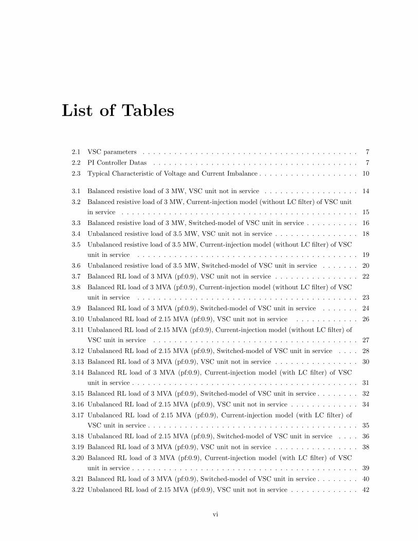
List of Tables

2.1 VSC parameters . . . . . . . . . . . . . . . . . . . . . . . . . . . . . . . . . . . . . . . . . 7

2.2 PI Controller Datas . . . . . . . . . . . . . . . . . . . . . . . . . . . . . . . . . . . . . . . 7

2.3 Typical Characteristic of Voltage and Current Imbalance . . . . . . . . . . . . . . . . . . . 10

3.1 Balanced resistive load of 3 MW, VSC unit not in service . . . . . . . . . . . . . . . . . . 14

3.2 Balanced resistive load of 3 MW, Current-injection model (without LC filter) of VSC unit

in service . . . . . . . . . . . . . . . . . . . . . . . . . . . . . . . . . . . . . . . . . . . . . 15

3.3 Balanced resistive load of 3 MW, Switched-model of VSC unit in service . . . . . . . . . . 16

3.4 Unbalanced resistive load of 3.5 MW, VSC unit not in service . . . . . . . . . . . . . . . . 18

3.5 Unbalanced resistive load of 3.5 MW, Current-injection model (without LC filter) of VSC

unit in service . . . . . . . . . . . . . . . . . . . . . . . . . . . . . . . . . . . . . . . . . . 19

3.6 Unbalanced resistive load of 3.5 MW, Switched-model of VSC unit in service . . . . . . . 20

3.7 Balanced RL load of 3 MVA (pf:0.9), VSC unit not in service . . . . . . . . . . . . . . . . 22

3.8 Balanced RL load of 3 MVA (pf:0.9), Current-injection model (without LC filter) of VSC

unit in service . . . . . . . . . . . . . . . . . . . . . . . . . . . . . . . . . . . . . . . . . . 23

3.9 Balanced RL load of 3 MVA (pf:0.9), Switched-model of VSC unit in service . . . . . . . 24

3.10 Unbalanced RL load of 2.15 MVA (pf:0.9), VSC unit not in service . . . . . . . . . . . . 26

3.11 Unbalanced RL load of 2.15 MVA (pf:0.9), Current-injection model (without LC filter) of

VSC unit in service . . . . . . . . . . . . . . . . . . . . . . . . . . . . . . . . . . . . . . . 27

3.12 Unbalanced RL load of 2.15 MVA (pf:0.9), Switched-model of VSC unit in service . . . . 28


3.14 Balanced RL load of 3 MVA (pf:0.9), Current-injection model (with LC filter) of VSC

unit in service . . . . . . . . . . . . . . . . . . . . . . . . . . . . . . . . . . . . . . . . . . . 31

3.15 Balanced RL load of 3 MVA (pf:0.9), Switched-model of VSC unit in service . . . . . . . . 32

3.16 Unbalanced RL load of 2.15 MVA (pf:0.9), VSC unit not in service . . . . . . . . . . . . . 34

3.17 Unbalanced RL load of 2.15 MVA (pf:0.9), Current-injection model (with LC filter) of

VSC unit in service . . . . . . . . . . . . . . . . . . . . . . . . . . . . . . . . . . . . . . . . 35



3.20 Balanced RL load of 3 MVA (pf:0.9), Current-injection model (with LC filter) of VSC

unit in service . . . . . . . . . . . . . . . . . . . . . . . . . . . . . . . . . . . . . . . . . . . 39

3.21 Balanced RL load of 3 MVA (pf:0.9), Switched-model of VSC unit in service . . . . . . . . 40

3.22 Unbalanced RL load of 2.15 MVA (pf:0.9), VSC unit not in service . . . . . . . . . . . . . 42

vi

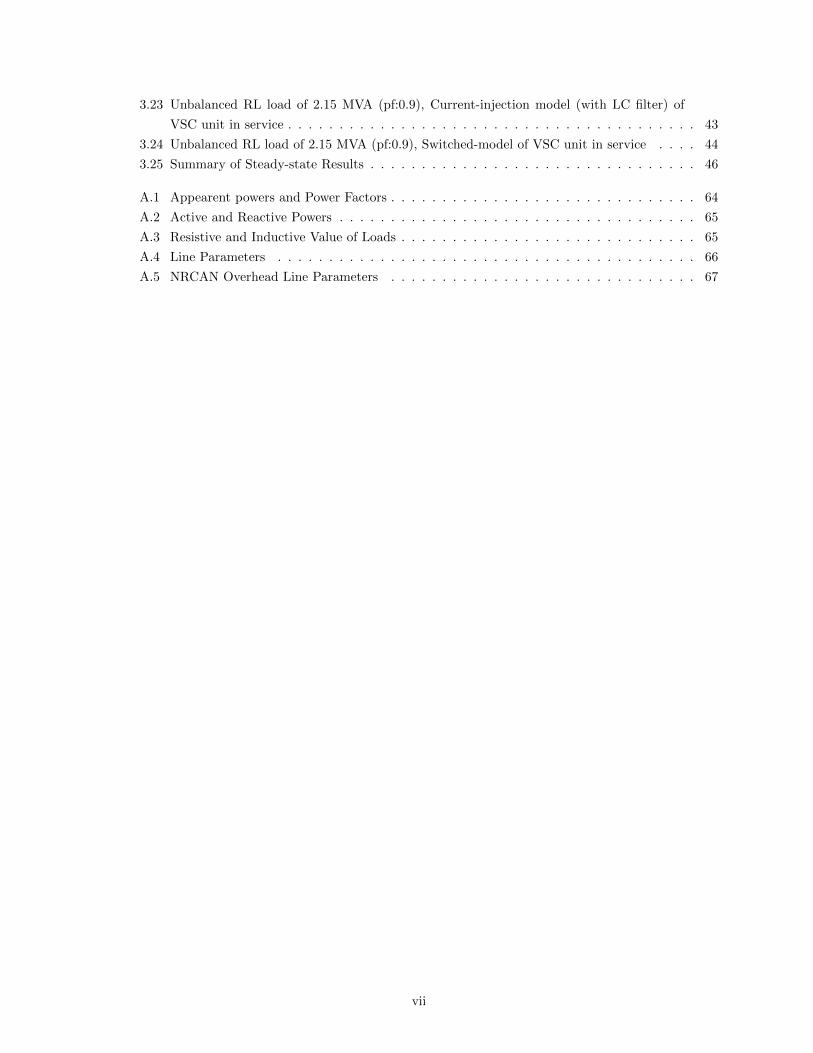
3.23 Unbalanced RL load of 2.15 MVA (pf:0.9), Current-injection model (with LC filter) of

VSC unit in service . . . . . . . . . . . . . . . . . . . . . . . . . . . . . . . . . . . . . . . . 43


3.25 Summary of Steady-state Results . . . . . . . . . . . . . . . . . . . . . . . . . . . . . . . . 46

A.1 Appearent powers and Power Factors . . . . . . . . . . . . . . . . . . . . . . . . . . . . . . 64

A.2 Active and Reactive Powers . . . . . . . . . . . . . . . . . . . . . . . . . . . . . . . . . . . 65

A.3 Resistive and Inductive Value of Loads . . . . . . . . . . . . . . . . . . . . . . . . . . . . . 65

A.4 Line Parameters . . . . . . . . . . . . . . . . . . . . . . . . . . . . . . . . . . . . . . . . . 66

A.5 NRCAN Overhead Line Parameters . . . . . . . . . . . . . . . . . . . . . . . . . . . . . . 67

vii

List of Figures

2.1 One-line Diagram of the Study System . . . . . . . . . . . . . . . . . . . . . . . . . . . . . 5

2.2 One-line Diagram of the Study System represented by two equivalents with respect to

right- and left-side of POI . . . . . . . . . . . . . . . . . . . . . . . . . . . . . . . . . . . . 6

2.3 Schematic Diagram of the VSC . . . . . . . . . . . . . . . . . . . . . . . . . . . . . . . . . 6

2.4 Inner-loop Current Controller . . . . . . . . . . . . . . . . . . . . . . . . . . . . . . . . . . 7

2.5 VSC current-sourced model . . . . . . . . . . . . . . . . . . . . . . . . . . . . . . . . . . . 8

2.6 Integration of Current-Sourced Model of VSC with the host AC system . . . . . . . . . . 9

2.7 Current-Controlled Voltage-Source Model . . . . . . . . . . . . . . . . . . . . . . . . . . . 9

3.1 One-Line Diagram of the Study System . . . . . . . . . . . . . . . . . . . . . . . . . . . . 12

4.1 LLL fault, Current-Injection Model . . . . . . . . . . . . . . . . . . . . . . . . . . . . . . . 48

4.2 LLL fault, Current-Injection Model . . . . . . . . . . . . . . . . . . . . . . . . . . . . . . 49

4.3 LLL Fault, Switched-model . . . . . . . . . . . . . . . . . . . . . . . . . . . . . . . . . . . 50

4.4 LLL Fault, Switched-model . . . . . . . . . . . . . . . . . . . . . . . . . . . . . . . . . . . 50

4.5 LG Fault, Current-Injection Model . . . . . . . . . . . . . . . . . . . . . . . . . . . . . . . 52

4.6 LG Fault, Current-Injection Model . . . . . . . . . . . . . . . . . . . . . . . . . . . . . . . 52

4.7 LG Fault, Switched-model . . . . . . . . . . . . . . . . . . . . . . . . . . . . . . . . . . . . 53

4.8 LG Fault, Switched-model . . . . . . . . . . . . . . . . . . . . . . . . . . . . . . . . . . . . 53

4.9 LLG Fault, Current-Injection model . . . . . . . . . . . . . . . . . . . . . . . . . . . . . . 55

4.10 LLG Fault, Current-Injection model . . . . . . . . . . . . . . . . . . . . . . . . . . . . . . 55

4.11 LLG Fault, Switched-model . . . . . . . . . . . . . . . . . . . . . . . . . . . . . . . . . . . 56

4.12 LLG Fault, Switched-model . . . . . . . . . . . . . . . . . . . . . . . . . . . . . . . . . . . 56

4.13 LL Fault, Current-Injection Model . . . . . . . . . . . . . . . . . . . . . . . . . . . . . . . 58

4.14 LL Fault, Current-Injection Model . . . . . . . . . . . . . . . . . . . . . . . . . . . . . . . 58

4.15 LL Fault, Switched-model . . . . . . . . . . . . . . . . . . . . . . . . . . . . . . . . . . . . 59

4.16 LL Fault, Switched-model . . . . . . . . . . . . . . . . . . . . . . . . . . . . . . . . . . . . 59

viii

List of Abbreviations

VSC Voltage Source Converter

SCR Short-Circuit Ratio

PLL Phase Locked Loop

DG Distributed Generation

VSC Voltage Source Converter

DN Distribution Network

AMI Advanced Metering/Monitoring Infrastructure

VAR Volt-Ampere Reactive

DC Direct Current

AC Alternating Current

HVDC High-Voltage Direct Current

SCMVA Short Circuit MVA

POI Point of Interconnection

SPWM Sinusoidal Pulse Width Modulation

IEEE Institute of Electrical and Electronics Engineers

LV Low Voltage

NEMA National Equipment Manufacturer’s Association

LVUR Line Voltage Unbalance Rate

PVUR Phase Voltage Unbalance Rate

ix

Chapter 1

Introduction

1.1 Problem Statement

Recent and ongoing developments in power electronics economical viability of alternative energy re-

sources, e.g., wind and solar power [1, 2], and energy storage media, e.g., battery and flywheel storage sys-

tems, all indicate significant proliferation of voltage-sourced converter (VSC) units in the electric power

grid [3]-[6]. In this context, the VSC serves as the electrical interface medium between a source/storage

system and it host utility grid. Depending on the rated power and functions of the source/storage sys-

tem, the corresponding VSC unit can be either a single-phase or three-phase unit. This documents is

concerned with three-phase VSC units. The three-phase VSC unit has been widely used to interface a

source/storage system of few tens of kW up to multi-MW at voltage levels of a few hundred volts to

tens of kV. Except for HVDC system applications, a VSC is cascaded with a three-phase transformer

which can have a variety of winding configurations.

The inherent operational characteristic of the VSC enables it to provide fast control over multiple

parameters, e.g., instantaneous real/reactive power (PQ mode), DC side voltage, AC side voltage phasor,

and frequency [7, 8]. This document is concerned with the scenarios that a VSC operates in the PQ-

mode and can inject/absorb real- and reactive-power in four quadrants. This mode is the most widely

adopted mode of operation at the distribution-class voltage levels, e.g., 480-V to 69-kV, and includes

VSCs from a few tens of kW up to 2.5 MW.

For the utility grid applications, a VSC can be operated either as a voltage-controlled unit or a

current-controlled unit with respect to the AC side. The latter is the preferred mode since it provides

current-limit capability and provides embedded over-current protection for the electronic switches during

the utility grid abnormal scenarios, e.g., faults and switching events. In this document we adopt the

VSC under the current-controlled mode of operation in which the inner current control-loop controls

the injected current by the VSC into the grid and the outer control loop provides the required current

reference values to meet PQ exchange of the overall unit, i.e., the source/storage and the VSC interface.

The underlying assumption in the VSC modeling, control, and performance evaluation by the vendors

and power utilities is that the host grid is a three-phase balanced system. This is a fairly valid assumption

for three-phase transmission-level system but not for the distribution level systems. The distribution-

level system is subject to a significant degree of asymmetry under steady-state conditions due to (i)

untransposed lines, single-phase laterals,and single-phase load and/or generation. This asymmetry is

1

even more pronounced under transient scenarios, e.g., a single-phase to ground fault and its subsequent

single-pole breaker operation and re-closure actions.

Prior to installation, commisioning, and operation of a VSC-interfaced generation/storage unit, the

power utility performs multiple impact studies to guarantee sound operation of the unit its host grid

under a wide range of system scenarios. These studies conventionally utilize the positive-sequence based

vendor model of the VSC and its control which is designed under the assumption of balanced grid.

Therefore, the main concern that has been raised by the utility industry includes:

• Do positive-sequence based generic models of the VSC [9] (and its control) provide adequately

accurate response under (realistic) unbalanced conditions of the distribution grid ?

• Is there a specific unbalanced threshold limit beyond which the positive-sequence based VSC models

are not adequately accurate ?

• Can the VSC be equipped with additional controller to (i) mitigate the impact of system unbalance

on the VSC operation, and/or (ii) even counteract the system unbalanced behavior?

The above issues have neither been fully answered in a systematic way nor been comprehensively un-

derstood, particularly where multiple VSC units operate in close electrical proximity of each other. The

focus of this work to address the first two concerns. Providing meaningful response to the latter question

requires establishment of ”performance criteria” which is beyond the scope of this work.

1.2 Thesis Objectives

The objectives of this work include:

(a) Identification of a realistic distribution system (feeder) down stream to the distribution transformer

station for the studies.

(b) Developing the steady-state power flow model and transient model of the system of item (a) (in the

PSCAD platform) for the required studies.

(c) Selection of a VSC-interfaced distributed generation system and development of its positive-sequence

model to be incorporated in the system models of item (b) above.

(d) Comprehensive case studies, under steady-state and transient scenarios, to establish the VSC re-

sponse under balanced and unbalanced conditions.

1.3 Thesis Layout

The structure of this thesis is as follows:

Chapter 2 introduce a distribution feeder which is used in the rest of the thesis for the case studies.

Chapter 2 also presents a generic structure for a three-phase VSC unit and its control to integrate

distributed generation/storage in the test feeder. Finally chapter 2 introduces widely used models of the

VSCs for the case studies.

Chapter 3 adopts the VSC models of chapter 2 and evaluates performance of models under steady

conditions and provides a comparison of performances.

2

Chapter 4 is primarily concerned with the performances of the VSC models of chapter 2 under

transient scenarios. Both balanced and unbalanced faults and the subsequent switching events are

considered.

Chapter 5 provides the conclusions of the studied cases and the future work in the area.

3

Chapter 2

Study System

2.1 Introduction

This chapter introduces distribution power system, i.e., a feeder down stream of a transformer station,

as the system that incorporates a VSC-interfaced generation unit [10, 11] for the study cases. This

chapter also introduces the details of the VSC-interfaced unit and its control system. The introduced

study system is used in the subsequent chapters to investigate the behavior of the VSC unit under the

distribution system balanced/unbalanced conditions [12, 13].

2.2 Distribution Feeder

Figure 2.1 shows a schematic diagram of the distribution feeder for the investigations [14, 15]. The

main trunk of the feeder is a 27.6 kV overhead line which is supplied by the main grid. The main

grid is represented in Figure 2.1 by an equivalent 27.6 kV voltage source with the short circuit capacity

(SCMVA) of 885.33 MVA. The feeder supplies multiple loads by lateral overhead lines either directly or

through transformers. Figure 2.1 also shows that the laterals can be three-phase, two-phase, and single-

phase [16, 17]. Therefore, the feeder is an unbalanced system. The main overhead line of the feeder is

not transposed and thus is not symmetrical. The feeder also includes a voltage regulating transformer,

i.e., transformer T2. The parameters of the feeder are given in Appendix A . The feeder is also equipped

with a three-phase 1.5 MW, 370 V distributed generation unit, e.g., a solar-PV unit, which is interfaced

to the feeder at the point of interconnection (POI) through a three-phase transformer and a three-phase

two-level VSC unit as will be described in the following sections.

For some study cases where the feeder characteristics at POI need to be re-adjusted to highlight the

impact of the specific scenarios, instead of the configuration of Figure 2.1, it equivalents with respect

to POI, as shown in Figure 2.2, are used. In the system of Figure 2.2, (i) the main system of Figure

2.1 and the feeder section between the main feeder and POI is replaced by its thevenin equivalent with

respect to POI, and (ii) the feeder downstream from POI is replaced by a passive impedance (assuming

there is no generation beyond POI in the feeder).

4

Figure 2.1: One-line Diagram of the Study System

5

Figure 2.2: One-line Diagram of the Study System represented by two equivalents with respect to right-and left-side of POI

2.3 Distributed Generation Unit

Figure 2.3 shows a schematic diagram of the distributed generation system [18], e.g., a solar-PV unit,

including its VSC-interface.

Figure 2.3: Schematic Diagram of the VSC

The DC-side is represented by (i) a DC voltage source, (ii) L and R, respectively, represent the

inductance and the equivalent internal resistance of the DC-side interface reactor, and (iii) DC-capacitor

C. The VSC is a conventional IGBT-based two-level configuration. The VSC operates based on a

sinusoidal pulse width modulation (SPWM) switching strategy at the switching frequency of 3.06 kHz.

The AC side filter is an LC filter in each phase to meet the IEEE harmonic content requirements [19]. It

should be noted that converter transformer also participates in the filter action and practically the filter

in each phase is an asymmetrical ”T” type filter [20]. The parameters of the configuration of Figure 2.3

are given Table 2.1.

6

Table 2.1: VSC parametersDC-side

Parameters ValuesL 1 uHR 20000 ohmC 12000 uF

AC-sideParameters Values

Lf 27 uHCf 2900 uF

Figure 2.4 shows a block diagram of the inner-loop current-controller of the VSC [12], and the outer-

loop control system determines the reference currents for the inner-loop, i.e., Idref and Iqref , based

on the desired control objective [8]. Presently, most electronically-coupled DG units operate based on

real- and reactive-power injection and this strategy is adopted in this work for the outer-controller. The

VSC unit is synchronized to the transformer low-voltage (LV) side by a phase-locked loop (PLL) system

[13, 21]. The PLL provides the synchronization to the positive-sequence voltage of the transformer low

voltage (LV) side.

Figure 2.4: Inner-loop Current Controller

Table 2.2: PI Controller DatasParameters Values

Proportional Gain 0.022Integral Time Constant 0.5 s

2.4 System Model

For the purpose of the studies reported in the following chapters, the overall system is modeled in the

EMTDC/PSCAD platform as follows.

7

2.4.1 Feeder Model

The feeder is represented as a three-phase system (and two-phase and single-phase where applicable).

Each line section is represented by lumped RL elements including sequence parameters. Each transformer

is represented as a linear three-phase transformer according to the corresponding winding structure of

Figure 2.1. The network equivalent in Figure 2.1 is represented by a three-phase voltage source including

sequence impedances. This modeling process also used when the feeder system of Figure 2.2 was used.

2.4.2 VSC System Switch-Model

The detailed converter system includes sections described in section 2.3. The power circuity of the

converter system, i.e., that of Figure 2.3, is modeled in the EMTDC/PSCAD platform, in which the

VSC electronic switches are represented as ideal on-off switches.The control system of the VSC converter,

i.e., those of Figures 2.4 and the outer-loop controller, including the synchronization PLL are modeled in

the EMTDC/PSCAD software tool. This model represents the dynamics of the converter system and in

steady-state conditions it provides both the fundamental-frequency response of the converter system and

the switching harmonics. Hereafter we refer to this model of the VSC system as the ”switched-model”

and it provides a benchmark for evaluation of the accuracy of the other VSC system models as described

in the following sections.

Figure 2.5: VSC current-sourced model

8

2.4.3 VSC Current-Sourced (Current-Injection) Model

In this modeling approach the VSC of Figure 2.3, excluding the AC-side filter, the inner-loop current

controller of Figure 2.4 and the outer real-/reactive-power controllers are combined and represented as

a current-controlled current-source as shown in Figure 2.5 which produce Id and Iq. This source injects

into the system, Figure 2.6, the three-phase current Ia, Ib, and Ic associated with the reference Id and

Iq current components that are generated by the model of Figure 2.5. Thus it injects currents into

the system associated with the desired real- and reactive-power components. Hereafter, this model is

referred to ”current-sourced model” or ”current-injection model”.

Figure 2.6: Integration of Current-Sourced Model of VSC with the host AC system

It should be noted that the current-sourced model represents the steady-state and dynamics of the

VSC system only at the fundamental frequency component of its AC side. The current-sourced model

of Figure 2.6 is widely adopted by the stakeholders to perform system impact studies. The objective of

this work is to establish if the response of this model accurately agrees with that of the switched-model

of section 2.4.2, particularly under unbalanced and/or low short-circuit ratio (SCR) conditions.

2.4.4 VSC Voltage-Sourced Model

Another option for an equivalent model of the VSC system is to represent it as a current-controlled

voltage source, as shown in Figure 2.7.

Figure 2.7: Current-Controlled Voltage-Source Model

The voltage source of Figure 2.7 is current-controlled such that it meets the requirements of active-

and reactive-power reference values and the inner-loop current controller. The main drawback of this

model as compared with that of Figure 2.6 is that it requires details of the inner-loop current controller

which often is not provided by the VSC vendor and thus is not used in this work any further.

9

2.5 Definition of System Unbalanced

The three widely used and common definitions of voltage unbalance are as follows.

NEMA (National Equipment Manufacturer’s Association) Definition : The NEMA defini-

tion of voltage imbalance also known as the line voltage unbalance rate (LVUR) [22] is given by

LV UR(%) =max voltage deviation from the average line voltage

average line voltage100. (2.1)

IEEE Definition: The IEEE definition [23] of voltage unbalance, also known as phase voltage

unbalance rate (PVUR) is given by

PV UR(%) =max voltage deviation from the average phase voltage

average phase voltage100. (2.2)

The IEEE definition of voltage unbalance is similar to that of NEMA, and the only difference is that

the IEEE uses phase voltage rather than the line-to-line voltage.

True Definition : This definition is expressed as the ratio of the negative-sequence voltage compo-

nent, to the positive-sequence voltage component, [19],[23]-[25],

unbalance(%) =Vnegative−sequence

Vpositive−sequence100. (2.3)

The true definition is used in this thesis because it is more widely used in the literature as compared

with the other two definitions. The typical characteristic of imbalance, based the true definition, are

given in Table 2.3.

Table 2.3: Typical Characteristic of Voltage and Current ImbalanceSystem Condition Voltage and current

MagnitudeVoltage imbalance steady-state 2%Current imbalance steady-state 30%

2.6 Summary

This chapter introduces the test system and the corresponding component model for case studies in the

PSCAD/EMTDC platform. The test system is a 27-kV rural distribution feeder which includes multiple

three-, two- and single-phase loads and hosts a 1.5 MW VSC-interfaced distributed generation unit.

The unit is represented based on two models, i.e., the switched-model and the current-sourced model.

The switched-model is the most accurate representation for system studies within the frequency range

of about 0-50 khz while the current-sourced model only represents the fundamental-frequency behaviour

of the unit.

10

Chapter 3

Steady-State Responses of VSC

Models

3.1 Introduction

The objectives of this chapter is to investigate the behavior of a three-phase, three wires, inverter-

interfaced unit under unbalanced, steady-state system conditions. The study system is the rural dis-

tribution feeder introduced in the Chapter 2 and its single-line diagram is repeated in Fig. 3.1 for the

ease of reference. The VSC-integrated system is the 1.5 MW, 370 V system that was also introduced

in Chapter 2. The inverter-based system is represented by two modals, i.e., the switched-model and

the current-injection modal in the PSCAD/EMTDC software platform. The corresponding results are

compared to establish the degree of accuracy of the current-injection model as compared with detailed

switched-model, with report to the fundamental frequency component

11

Figure 3.1: One-Line Diagram of the Study System

12

3.2 Component Models

The reported studies in this chapter are based on time-domain simulation of the study system of Figure

3.1 in the PSCAD/EMTDC platform. The components of the study system of Figure 3.1 are developed

in the PSCAD/EMTDC as described in Chapter 2. For each case study, the VSC of unit is represented

once by the switched-model and once by the current-injection model. Since the switched-model captures

the details of the VSC behaviour, its response is used as the reference. Comparison of the results from

the VSC current-injection model with those of the switched-model are used to evaluate the accuracy of

the current-injection model.

3.3 Study Results

For each of the two models of the VSC unit, the studies are conducted for various scenerios that pratically

can be experienced, i.e.,

• balanced or unbalanced load conditions,

• (almost) resistive or RL loads,

• different values of short-circuit capacity at POI of Figure 3.1

The results are tabulated and compared in the following sections. In the reported studies, the degree

of the system imbalance of the voltage (current) is specified by the ratio of the negative-sequence voltage

(current) amplitude to the positive-sequence voltage (current) amplitude [19], [23]-[25] and the acceptable

limits are provided in Table 2.2 of Chapter 2. To create a specific level of ”unbalanced” at POI, the

down-stream load with respect to POI is made unbalanced, e.g., corresponding to 2% unbalanced voltage

at POI.

3.3.1 Case-1 : Short-Circuit Capacity of 85 MVA at POI

The main grid short-circuit MVA (SCMVA) at the distribution substation is about 885 MVA. Due to

the feeder impedance between the substation and POI of Fig. 3.1, the SCMVA at POI is 85 MVA.

Case-1.1 : Balanced Resistive Load (3 MW)

Table 3.1 shows the study results under the balanced resistive loads of 3 MW (downstream to POI)

when the VSC unit is not in service. Table 3.1 indicates, as expected, the three phase POI voltages are

balanced. Table 3.1 also shows various measured currents/voltages of the study system which are used

as the base cases to evaluate the impact of system unbalanced operation.

Table 3.2 shows the study results when the same resistive balanced load of 3 MW is in service, and

current-injection model (without LC filter) of VSC unit is connected at POI, as shown in Figure 3.1.

Table 3.2 indicates that, as expected, the three-phase POI voltages remain balanced.

Table 3.3 illustrates the study results under the same resistive balanced load of 3 MW when the

switched-model of VSC unit is connected to the main feeder at POI. Similar to the two previous cases

of Table 3.1 and Table 3.2, the results of Table 3.3 also indicate that voltages of the three-phase at POI

are balanced.

13

Table 3.1 to 3.3 conclude that for the given system SCMVA = 85 both models provide practically

identical results and thus the current-injection model accurately represents the VSC.

Table 3.1: Balanced resistive load of 3 MW, VSC unit not in service

14

Table 3.2: Balanced resistive load of 3 MW, Current-injection model (without LC filter) of VSC unit inservice

15

Table 3.3: Balanced resistive load of 3 MW, Switched-model of VSC unit in service

16

Case-1.2 : Unbalanced Resistive Load (3.5 MW)

In this case study, the overall load of the feeder is adjusted to 3.5 MW which correspond to 1 MW

single-phase load (phase A) and 2.5 MW two-phase load connected to phases B and C to make system

unbalance. Table 3.4 shows the study results under the unbalanced resistive load of 3.5 MW when the

VSC unit is not in service. Due to the unbalanced loads, the degree of POI voltage imbalance is 1.91%,

and the degree of current imbalance is 37.06%.

Table 3.5 shows the study results for the same unbalanced resistive load when the VSC unit is in

service and represented by the current-injection model (without LC filter), and injects 1.5 MW power

in the system at POI. Table 3.5 shows that in spite of the presence of the VSC unit in the system,

the voltage imbalance at POI remains identical to that of the previous case, as shown in Table 3.4.

However, the degree of current imbalance (current from source to POI) increased from 37.06% (Table

3.4) to 67.52% (Table 3.5). The reason is that part of the balanced-current of the load is supplied by the

VSC unit, and thus the balanced-current drawn by the load from the grid, through positive-sequence

current at branch form source to POI is reduced, and thus the degree of imbalance is increased.

Table 3.6 presents the study results corresponding to the previous scenerio when the VSC unit is

represented by the switching-model for the studies. Comparison of the results of Table 3.5 and 3.6

indicates that:

• the degrees of voltage imbalance at POI for both cases are practically the same, i.e. 1.91%.

• the degrees of current imbalance (from source to POI) for both cases are the same, i.e. 67.8%.

Table 3.4 and 3.6 conclude that both models of the VSC unit, subject to resistive unbalanced load

scenarios, under steady-state conditions, behave the same and can be used interchangebly.

17

Table 3.4: Unbalanced resistive load of 3.5 MW, VSC unit not in service

18

Table 3.5: Unbalanced resistive load of 3.5 MW, Current-injection model (without LC filter) of VSCunit in service

19

Table 3.6: Unbalanced resistive load of 3.5 MW, Switched-model of VSC unit in service

20

Case-1.3 : Balanced RL Load (3 MVA, 0.9 lagging power factor)

The study results presented in Table 3.7 correspond to balanced RL (resistance-inductance) load of 3

MVA at lagging power factor of 0.9 when the VSC unit is not in service. Table 3.7 shows, as expected,

the three-phase voltage at POI is balanced.

Table 3.8 and Table 3.9 show the study results under the same grid condition and the same load

connection of Table 3.7 when the VSC unit is in service and represented by the current-injection model

(without LC filter) and switched-model with 1.5 MW power injection at POI. Table 3.8 and Table 3.9

indicate, as expected, the three-phase POI voltages remain balanced. Close agreement between the

corresponding results of Table 3.8 and Table 3.9 indicates that current-injection model is an accurate

representation of the VSC for the given scenario.

21

Table 3.7: Balanced RL load of 3 MVA (pf:0.9), VSC unit not in service

22

Table 3.8: Balanced RL load of 3 MVA (pf:0.9), Current-injection model (without LC filter) of VSCunit in service

23

Table 3.9: Balanced RL load of 3 MVA (pf:0.9), Switched-model of VSC unit in service

24

Case-1.4 : Unbalanced RL Load (2.15 MVA, 0.9 lagging power factor)

For this case, the total load of the feeder is adjusted to 2.15 MVA at 0.9 lagging power factor which

corresponds to 1 MVA single-phase load (at phase A) and 1.15 MVA two-phase load connected to phases

B and C.

The study results of Table 3.10 correspond to the unbalanced RL load of 2.15 MVA (0.9 lagging

power factor) when the VSC unit is not in service. Due to unbalanced load, Table 3.10 shows that the

degree of voltage imbalance at POI is 1.97%, and the degree of current imbalance (from source to POI)

is 37.8%.

Table 3.11 shows the study results under the same unbalanced RL load when the VSC unit is in

service, and represented by current-injection model (without LC filter), and injects 1.5 MW power in

the system at POI. Table 3.11 indicates that the degree of voltage imbalance at POI is 1.96%. Despite

of the presence of the VSC unit in the system, voltage results of Table 3.10 and 3.11 are practically the

same. However, the degree of current imbalance (from source to POI) is increased from 37.8% (Table

3.10) to 61.36% (Table 3.11).

Table 3.12 presents the study results of the previous scenario under the same unbalanced RL load

when the VSC unit is represented by the switched-model, and injects 1.5 MW power in the system at

POI. A comparison of Table 3.11 and Table 3.12 shows that:

• The degree of voltage imbalance at POI changes from 1.96% (Table 3.11) to 1.97% (Table 3.12).

The difference between the two tables is negligible, and thus the results are practically the same.

• The degrees of current imbalance (from source to POI) for both cases are practically the same.

Similar to the previous case studies, Table 3.11 and Table 3.12 conclude that the current-injection

model is a valid representation of the VSC for the given scenario.

25

Table 3.10: Unbalanced RL load of 2.15 MVA (pf:0.9), VSC unit not in service

26

Table 3.11: Unbalanced RL load of 2.15 MVA (pf:0.9), Current-injection model (without LC filter) ofVSC unit in service

27

Table 3.12: Unbalanced RL load of 2.15 MVA (pf:0.9), Switched-model of VSC unit in service

28

3.3.2 Case-2 : Short-Circuit Capacity of 16.6 MVA at POI

The main grid short-circuit MVA (SCMVA) at the distribution substation is about 885 MVA. Due to

the feeder impedance between the substation and POI, the SCMVA at POI is 16.6 MVA. To reduce

short-circuit MVA from 85 to 16.6 at POI, source impedance value is increased. Practically this can

occur due to changes in the main grid configuration, e.g., when a transmission line is out of service.


Table 3.13 presents the study results under a balanced RL load of 3 MVA at 0.9 lagging power factor

(downstream to POI) when the VSC unit is not in service. Table 3.13 demostrates, as expected, the

three-phase voltages at POI are balanced.

Table 3.14 and Table 3.15 show the study results under the same balanced RL load of 3 MVA at 0.9

lagging power factor when the VSC unit is in service, and represented by the current-injection model

(with LC filter) and the switched-model at POI, respectively. In both cases, the VSC injected power in

the system is 1.5 MW. Table 3.14 and Table 3.15 indicate, as expected, the three-phase POI voltages

remain balanced, and the two VSC unit models have the same behaviour for this scenario.

29


30

Table 3.14: Balanced RL load of 3 MVA (pf:0.9), Current-injection model (with LC filter) of VSC unitin service

31


32


For this case, the same unbalanced load scenario of Case-1, Section 3.3.1, page 17 is used.

Table 3.16 presents the study results under unbalanced RL load of 2.15 MVA at 0.9 lagging power

factor when the VSC unit is not in service. Due to the unbalanced load, Table 3.16 indicates that the

degree of the voltage imbalance at POI is 2.15%, and the degree of current imbalance (from source to

POI) is 14.29%.

Table 3.17 shows the study results under the same unbalanced RL load when the VSC unit, which is

represented by the current-injection model (with LC filter), is in service and injects 1.5 MW power in the

system at POI. Table 3.17 demonstrates that the degree of voltage imbalance at POI is 2.17%. Although

the VSC unit is in service, the voltage imbalance results of the Table 3.16 and 3.17 are practically the

same. However, the degree of current imbalance (from source to POI) is increased from 14.29% (Table

3.16) to 32.61% (Table 3.17). The reason is the same as explained for Case-1, Section 3.3.1, page 28.

Table 3.18 presents the study results under the same unbalanced load when the VSC unit is repre-

sented by the switched-model, and injects 1.5 MW power in the system at POI. Comparing the results

of Table 3.17 and 3.18 indicates :

• The degrees of voltage imbalance at POI change from 2.17% (Table 3.17) to 2.16% (Table 3.18).

The results, as presented, are practically the same.

• The degrees of current imbalance (from source to POI) change from 32.61% (Table 3.17) to 28.09%

(Table 3.18). The results conclude that the current-injection model increases the degree of current

imbalance as compared with the switched-model. The reason is that the fixed impedance model

are used to present the loads, and for each model of converter are connected at POI, the voltage at

POI changes. Therefore, the current (from source to POI) is altered, and accordingly the degree

of current imbalance changes.

Table 3.16 to Table 3.18 conclude that both models of the VSC unit, subject to unbalanced RL load

scenario, produce noteably different results and may not be used interchangeably.

33


34

Table 3.17: Unbalanced RL load of 2.15 MVA (pf:0.9), Current-injection model (with LC filter) of VSCunit in service

35


36

3.3.3 Case-3 : Short-Circuit Capacity of 8.5 MVA at POI

The same method of Section 3.3.2 is used to change POI SCMVA from 85 to 8.5. The same scenarios of

Section 3.3.2 are also applied in this section to investigate voltage and current imbalance under the two

models of the VSC.


Table 3.19 shows the study results under the balanced RL load of 3 MVA at 0.9 lagging power factor

when the VSC unit is not in service. Table 3.19 exhibits, as expected, that the three-phase POI voltage

is balanced. Table 3.20 and 3.21 show the study results under the same balanced RL load when the

VSC unit is in service, and represented by the current-injection model (with LC filter) and the switched-

model, respectively, and injects 1.5 MW power in the system at POI. As anticipated, Table 3.19 to Table

3.21 indicate that both models of the VSC unit provide identical responses under balanced conditions.

37


38

Table 3.20: Balanced RL load of 3 MVA (pf:0.9), Current-injection model (with LC filter) of VSC unitin service

39


40


For this case, the unbalanced load of the feeder is adjusted to 2.15 MVA at 0.9 lagging power factor

similar to that of Case-1, Section 3.3.1, page 17. Table 3.22 introduces the study results under unbalanced

load of 2.15 MVA at 0.9 lagging power factor when the VSC unit is not in service. Table 3.22 shows

that the degree of voltage imbalance at POI is 2.17%, and the degree of current imbalance (from source

to POI) is 6.12%.

Table 3.23 shows the study results under the same unbalanced RL load when VSC unit is represented

by the current-injection model (with LC filter), and injects 1.5 MW power in the system at POI. Table

3.23 shows that the degree of the voltage imbalance at POI is 2.21%. In spite of the presence of the

VSC unit, the POI voltage imbalance of Table 3.22 and 3.23 are practically the same. However, the

degree of current imbalance (from source to POI) is increased from 6.12% (Table 3.22) to 15.79% (Table

3.23).The reason is the same as explained for Case-1, Section 3.3.1, page 28.

Table 3.24 shows the study results under the same unbalanced RL load when the VSC unit is

represented by the switched-model, and injects 1.5 MW power in the system at POI. The comparison of

Table 3.23 and 3,24 indicates that:

• The degrees of voltage imbalance at POI changes from 2.21% (Table 3.23) to 2.18% (Table 3.24)

which are practically the same.

• The degrees of current imbalance (from source to POI) change from 15.79% (Table 3.23) to 13.5%

(Table 3.24). The current-injection model of the VSC unit results in a higher level of negative

sequence current as compared with the switched-model of the VSC unit. The reason is the same

as explained in Section 3.3.2, page 36.

The results of Table 3.22, 3.23 and 3.24 conclude that the two models of the VSC unit generate

different results however the differences are not significant.

41


42

Table 3.23: Unbalanced RL load of 2.15 MVA (pf:0.9), Current-injection model (with LC filter) of VSCunit in service

43


44

3.3.4 Case-4 : Short-Circuit Capacity of Less Than 8.5 MVA at POI

The Short-circuit ratio (SCR) of buses, at the transmission voltage levels, practically can be as low as

unity (or even less). However, in distribution systems the SCR value is often larger than unity. For

example, for the reported case studies of Section 3.3.1 to Section 3.3.3, the SCR value changes from

85/1.5 = 56.66 to 8.5/1.5 = 5.66.

For urban distribution feeders, the SCR value at different buses on the feeder is often significantly

higher than 5 and thus one can conclude that the switched-model and current-injection model of the VSC

provide (practically) identical results. However, the rural distribution feeders are (i) significantly longer

(up to even 60-km) than urban feeders, and (ii) supply highly sparse loads and thus the conductors have

higher impedances. Thus the SCMVA at buses close to the end of the feeder can be fairly low and as a

result the SCR value can be less than 5.

To compare the effects of the two VSC models on the POI voltage imbalance, three different values

of SCR, i.e., 6/1.5 = 4, 4.5/1.5 = 3 and 2.25/1.5 = 1.5 are considered and the results are as follows.

Case-4.1 : Unbalanced RL Load (2.15 MVA, 0.9 lagging power factor, SCR = 4)

For this scenario, the degree of POI voltage imbalance for the switched-model (current-injection model)

are 2.34 (2.24), 2.28 (2.23) and 2.39 (2.21). The reason for the noticeable difference between the corre-

sponding results is that the injected current harmonic in the system by the switched-model distorts the

POI voltages.

Case-4.2 : Unbalanced RL Load (2.15 MVA, 0.9 lagging power factor, SCR = 3)

In this case, the degree of POI voltage imbalance for the switched-model (current-injection model) are

3.18 (2.32), 3.41 (2.18) and 2.82 (2.26). There are two factors which contribute to the higher degree

of voltage imbalance of the switched-model, i.e., distortion due to harmonics and negative-sequence

component. The fidelity of the PLL used by the VSC for synchronization, i.e., the extend that the

PLL is immune to the effect of negative-sequence voltage component and harmonics becomes a main

consideration in this regard.

In practice, as of now, there is no specific standard/requirements on the PLL specifications. Therefore,

although the injection-model results are ”better” than the switched-model, they are pessimistic and can

be misleading. Therefore, the injection-model is not recommended for SCR = 3.

Case-4.3 : Unbalanced RL Load (2.15 MVA, 0.9 lagging power factor, SCR = 1.5)

For this scenario, the switched-model fails. The reason is that the PLL cannot handle the harmonic

distortion and cannot synchronize the VSC to the system. The injection-model, however, provide voltage

imbalance degrees of 2.35, 2.62, and 2.28 at POI. It should be noted that the switched-model results

(failure to operate) is potentially more realistic than those of the injection-model.

3.4 Conclusions

This chapter provided a comprehensive steady-state performance calculation of the behaviour of a VSC-

interfaced distributed resource unit under different SCR values and unbalanced conditions of the host

45

distribution system. The switched-model of the VSC is used as the benchmark (reference) model for

evaluation of the results obtained from current-injection (or current-sourced) model.

The study results show that:

• When the SCR at the point of interconnection (POI) of the VSC unit is larger than 5, i.e., short-

circuit capacity of the system is larger than 8.5-MVA, and the POI voltage imbalance within 2%,

the current-injection model reproduces the same results (at the fundamental frequency) as those

of the switched-model. Thus the two models can be used interchangeably.

• Under the above conditions, the presence of VSC unit can result in the high (67%) current unbal-

ance, upstream to POI, which can violate the acceptable limits. However, this is a bi-product of

the VSC-interfaced power generation property and not the model used to represent the VSC.

• When the SCR at POI becomes less than 5 and the voltage imbalance is within 2%, the difference

between the corresponding results of the two VSC models become noticeable. The main reason

is the impact of harmonics generated by the switched-model and the POI negative-sequence volt-

age on the behaviour of the VSC PLL. Since the current-injection does not generate harmonics,

the corresponding PLL behaves ”better”. Thus, the results from the current-injection model are

optimistic and necessarily not reliable.

• At very low SCR values, e.g., SCR ≤ 2, the switched-model fails to operate. This is due to inability

of the PLL to provide proper synchronization. However, the current-injection model can provide

synchronization. The inability of the VSC switched-model to operate is more realistic and the

results from the VSC current-injection model are not acceptable.

Table 3.25: Summary of Steady-state Results

46

Chapter 4

Transient Responses of VSC Models

4.1 Introduction

Chapter 3 investigated the steady-state behaviour of the switched-model and the current-injection model

of a three-phase VSC-interfaced distributed resource, under balanced and unbalanced conditions. The

main objective of this chapter is to evaluate and compare the corresponding responses of the two models

during and subsequent to the system transients, e.g., faults. The same study system of chapter 3 is

used in this chapter. The VSC unit is the 1.5 MW, 370 V system that was also presented in Chapter

2 and Chapter 3. The reported studies in this chapter are based on time-domain simulation studies of

the study system in the PSCAD/EMTDC platform.

4.2 Case Studies

The reported studies are for the case that (i) the load is a balanced RL at 0.9 lagging power factor, (ii)

the POI short-circuit capacity is 16.6 MVA, (iii) the VSC injects 1.5 MW into the system, (iv) the bus

voltage of the study system are within 0.95 to 1.05 per unit. The transient in the system are due to

faults which are occurred the same location that is bus B11 of Figure 3.1. The imbalance in the system

is due to asymmetrical faults, e.g., LG faults. Four different fault conditions were investigated, i.e.,

• line-to-line-to-line (LLL) fault, with the fault impedance of 0.01 ohm,

• line-to-line-to-ground (LLG) fault, with the fault impedance of 0.01 ohm,

• line-to-ground (LG) fault, with the fault impedance of 0.01 ohm,

• line-to-line (LL) fault, with the fault impedance of 0.01 ohm.

Each fault is imposed at time t = 0.1 s and self-cleared at time t = 0.25 s at the first current

zero-crossing for each phase.

4.2.1 LLL Fault

Figures 4.1 and 4.2 show the voltage and current waveforms respectively, for pre-fault, fault and post-

fault periods when the VSC is represented by the current-injection model. Figures 4.3 and 4.4 show the

voltage and current waveforms when the VSC is represented by the switched-model.

47

Figure 4.1: LLL fault, Current-Injection Model

(a) POI instantaneous line-to-line voltages

(b) POI instantaneous line-to-ground voltages

(c) 370-V side instantaneous line-to-line voltages

(d) POI rms line-to-line voltages

(e) POI rms line-to-ground voltages

(f) 370 V side rms line-to-line voltages

48

Figure 4.2: LLL fault, Current-Injection Model

(g) Source to POI instantaneous currents

(h) POI to load instantaneous currents

(i) VSC 27.6 kV side instantaneous currents

(j) VSC 370 V side instantaneous currents

(k) Source to POI rms currents

(l) POI to load rms currents

(m) VSC 27.6 kV side rms currents

(n) VSC 370 V side rms currents

49

Figure 4.3: LLL Fault, Switched-model

Figure 4.4: LLL Fault, Switched-model

50

Comparison of Figure 4.1 with the corresponding Figure 4.3 indicates that;

• Waveforms of line-to-line and line-to-ground voltages at POI are nearly the same. The peak

values of the POI line-to-ground voltage, after the fault is cleared, are 26.3 kV for the current-

injection model (Figure 4.1) and 24.6 kV for the switched-model (Figure4.3), respectively. Thus,

the current-injection results in a higher peak value of POI line-to-ground voltage.

• During the system LLL fault, line-to-line voltages (at 370 V side) are different in Figure 4.1 and in

Figure 4.3. Line-to-line voltages (at 370-V side) in Figure 4.1 have high frequency oscillations and

the rms values of the three Line-to-line voltages are not equal either. When the fault occurs, the

current-injection model, with respect to the rest of the system, is equivalent to a three-phase open-

circuit and the high frequency oscillations are caused by the LC filter resonance. The switched-

model during the fault is equivalent to a current-injecting voltage-source and thus do not exhibit

the effect of system LC resonance. The recovery peak voltages after the LLL fault is cleared for

the current-injection model and the switched-model are almost equal to 0.58-kV.

Comparison of Figure 4.2 with Figure 4.4 indicates that;

• The current waveforms (from source to POI) and (from POI to the load) are nearly the same.

During the LLL fault, the major parts of these currents are flowing from the source to the fault,

and the difference caused by the current-injection model and the switched-model are relatively

insignificant.

• Amplitudes of the current waveforms (at VSC 27.6-kV side) in Figure 4.2 and 4.4 are nearly the

same, but the waveforms in Figure 4.2 exhibit high frequency components. The reason is that

during the LLL fault the current-injection model is equivalent to the three-phase open-circuit, so

the LC filter causes the high frequency oscillations.

• The current peak values are 6.6 kA (in Figure 4.2) for the current-injection model and 6.3 kA (in

Figure 4.4) for the switched-model. The waveforms in Figure 4.2 also exhibit higher frequency

components.

Figure 4.1, 4.2, 4.3 and 4.4 conclude that both VSC models under the balanced RL load scenario,

provide notably different transient responses due to LLL fault, and necessarily cannot be used inter-

changeably.

4.2.2 LG Fault

Figures 4.5 and 4.6 show the voltage and current waveforms respectively, for pre-fault, fault and post-

fault periods when the VSC is represented by the current-injection model. Figures 4.7 and 4.8 show

the voltage and current waveforms, for the same fault scenario, when the VSC is represented by the

switched-model.

51

Figure 4.5: LG Fault, Current-Injection Model

Figure 4.6: LG Fault, Current-Injection Model

52

Figure 4.7: LG Fault, Switched-model

Figure 4.8: LG Fault, Switched-model

53

Comparison of Figures 4.5 and 4.7 conclude:

• The waveforms of line-to-ground voltages at POI nearly have the same patterns of variations for

both models. The peak values of the recovery line-to-ground voltages at POI are 27.9 kV (Figure

4.5) for the current-injection model and 24.8 kV (Figure 4.7) for the switched-model, and the

current-injection model results in significantly higher peak values of POI line-to-ground voltage.

• The peak values of the recovery voltages after the fault clearence are 0.66 kV (in Figure 4.5) and

0.58 kV (in Figure 4.7). Figure 4.5 also shows higher oscillations due to equivalent current source

behaviour as explained in Section 4.2.1, page 56.

Comparison of the corresponding results in Figures 4.6 and 4.8 reveal that:

• The waveforms of currents (from the source to POI and the VSC 27.6-kV side) are almost the

same for both models, and the difference in the peak values of the currents is negligiable.

• The peak values of current (at 370-V side) is 3.53 kA (Figure 4.6) for the current-injection model

and 3.65 kA (Figure 4.8) for the switched-model.

Figures 4.5, 4.6, 4.7 and 4.8 conclude that both VSC models under the balanced RL load scenario,

produce notably different results under the LG fault.

4.2.3 LLG Fault

Figures 4.9 and 4.10 show the voltage and current waveforms respectively, for the pre-fault, fault and

post-fault periods when the VSC is represented by the current-injection model. Figures 4.11 and 4.12

show the voltage and current waveforms when the VSC is represented by the switched-model.

54

Figure 4.9: LLG Fault, Current-Injection model

Figure 4.10: LLG Fault, Current-Injection model

55

Figure 4.11: LLG Fault, Switched-model

Figure 4.12: LLG Fault, Switched-model

56

Comparing to the corresponding waveforms from Figures 4.9 and 4.11 observes that:

• Instantaneous waveforms of the line-to-ground voltages at POI exhibit similar patterns of variation.

However, the peak values of POI line-to-ground voltage is 27.2 kV (Figure 4.9) for the current-

injection model and 24.3 kV (Figure 4.11) for the switched-model, and similar to the previous cases

the current-injection model results in higher peak value.

• The line-to-line voltages (at 370-V side) are different. The line-to-line voltages (at 370-V side) of

Figure 4.9 include higher oscillatory voltage components. Furthermore, the peak values of recovery

voltages are 0.65 kV (Figure 4.9) and 0.57 kV (Figure 4.11), and the current-injection model results

in higher peak values.

Comparison of the results from Figures 4.10 and 4.12 concludes:

• The current waveforms (from the source to POI and the VSC 27.6-kV side) are almost the same,

and the differences in the peak values of the currents are negligiable.

• The peak values of currents (at 370-V side) are 5.03 kA (Figure 4.10) and 4.84 kA (Figure 4.12),

and the waveforms in Figure 4.10 have high oscillatory components.

The study results of Figures 4.9 to 4.12 indicate the two VSC models, subject to the LLG fault,

result in noticeably different results and cannot be used interchangeably.

4.2.4 LL Fault

Figures 4.13 and 4.14 show the voltage and current waveforms respectively, for the pre-fault, fault and

post-fault periods when the VSC is represented by the current-injection model. Figures 4.15 and 4.16

show the voltage and current waveforms when the VSC is represented by the switched-model.

57

Figure 4.13: LL Fault, Current-Injection Model

Figure 4.14: LL Fault, Current-Injection Model

58

Figure 4.15: LL Fault, Switched-model

Figure 4.16: LL Fault, Switched-model

59

Comparison of the voltage waveforms (Figures 4.13 and 4.15) indicates that:

• Instantaneous waveforms of the line-to-ground voltages at POI exhibit similar patterns of varia-

tions, however, the peak value of the POI line-to-ground voltage is 27 kV (Figure 4.13) for the

current-injection model and 24 kV (Figure 4.15) for the switched-model, and the current-injection

model results in higher peak values.

• Comparing the line-to-line voltages (at 370-V side) in Figure 4.13 with those of Figure 4.15 shows

that the line-to-line voltages in Figure 4.13 include higher oscillatory components. Another no-

ticeable difference is that the peak value of the recovery voltage is 0.66 kV (Figure 4.13) for the

current-injection and 0.57 kV (Figure 4.15) for the switched-model.

Comparison of Figure 4.14 and Figure 4.16 indicates that;

• The waveforms of currents (from the source to POI and the VSC 27.6-kV side) are almost the

same, and the difference in the peak values are negligiable.

• The peak value of the current (at 370-V side) is 4.6 kA (Figure 4.6) for the current-injection model

and 4.1 kA (Figure 4.8) for the switched-model.

Figures 4.13, 4.14, 4.15 and 4.16 conclude that both VSC models under the balanced RL load scenario,

produce noticeably different results under the LL fault.

4.2.5 Effect of SCR on the Transient Responses of the VSC Models

The study results of Figures 4.1 to 4.16 correspond to the scenario when the short-circuit capacity of

the POI is adjusted at 16.6 MVA. Similar studies to those Figures 4.1 to 4.16 also conducted when

the SCMVA was increased to 85 and reduced to 5. At higher values of SCMVA, the waveforms of the

corresponding currents and voltages produced by the two VSC models become more similar. However,

the current-injection model always exhibits oscillatory components due to the resonance of the VSC

filter.

As the short-circuit capacity of POI decreases, the corresponding waveforms of the two VSC models

exhibit more pronounced differences. At SCMVA = 8, the switched-model fails after the fault occurance.

The reason for the failure is the significant harmonic content and distortion of the POI voltage which does

not permit the PLL successfuly synchronize the VSC with the POI fundemental component. However,

the current injection model can successfuly provide synchronization and operate after the fault inception.

At SCMVA = 5 both models fail and do not recover from the faulted condition. It should be noted that

more ellaborate PLL structures can be used to operate the VSC for even lower SCMVA values of the

POI. These PLL structures are used for VSC-based HVDC converters, but as of now not adopted for

distribution class VSC units.

4.3 Conclusions

This chapter evaluates and compares the corresponding time-domain responses of the switched-model and

the current-injection model of the 1.5-MW VSC-interfaced DG unit under the feeder fault scenarios.Four

fault scenarios, i.e., LLL, LG, LLG and LL are considered. Prior to a fault inception, the system is under

60

balanced conditions and the imbalance is created due to the fault asymmetry. Each fault is a temporary

fault for the duration of 0.15 s, and self-cleared at each phase current zero-crossing. The study results

are obtained from time-domain simulation of the system in the PSCAD/EMTDC platform.

The reported simulation results of Fig. 4.1 to Fig. 4.16 show that:

• Although the patterns of variations of the corresponding waveforms from both models show simi-

larity, however, the peak encountered values are noticeably different.

• The waveforms obtained from the current-injection model show oscillations due to resonance of

the system inductance and the capacitor of the VSC AC-side filter. However, such oscillations are

not observable in the switched-model responses. The reason is that the current-injection model

behaves as a current source (open-circuit) during the fault transients and thus forces the filter

capacitor to be in series with the system inductance. Thus oscillations at the natural frequency of

the capacitor and the net system induce occur.

• The deviation between the corresponding waveforms of the two model become more significant as

the SCR decreases, i.e., the system become ”weaker”.

• At SCR ≤ 8 the switched-model fails and cannot provide synchronization with the POI voltage.

The reason is the significant distortion of the POI voltage due to harmonic and the voltage negative-

sequence. The current-injection model can provide synchronization at SCR = 8 since it does

not inject harmonics in the system. However, failure of the switched-model is a more realistic

representation of the VSC unit and the results from the current-injection model are not reliable.

• For SCR values less than 5, both models fails due to the PLL failure to provide synchronization.

This chapter conclude that the results from the switched-model and the current-injection model, at

SCR values of 16 or less, are noticeably different and the two models cannot be used interchangeably.

61

Chapter 5

Conclusions

This work provides a comprehensive performance evaluation an comparison of two models of the VSC-

interfaced distributed resource units. The two models are the switched-model and the current-injection

model. The switched-model represents detailed switching instants of the VSC electronic switches and

thus provide accurate representation of the VSC and its control behaviour up to about 50 kHz. The

current-injection model (also called current-sourced model) represent the VSC and its controlled by a

three-phase current source that controls its injected current in the system based on the VSC inner-

current control strategy. The current-injection model only injects the fundamental frequency current

component in the system. The current-injection model is widely used by the electric power utilities

and the VSC manufacturers/vendors to investigate the impact of VSC-interfaced distributed resource

units on the utility grid. The main motivation of this work is to establish if the current-injection model

accurately represents the steady-state and dynamic behaviours of the VSC unit under different SCR

levels and degrees of system imbalance. The switched-model behaviour is used as the benchmark and

basis to establish the degree of accuracy/validity of the current injection model.

The reported studies are conducted on a typical 27.6-kV distribution feeder which includes a 1.5-MW

VSC-interfaced distributed generation unit. The studies are conducted based on time-domain simulation

in the PSCAD/EMTDC platform.

The study results of the steady-state responses of the VSC models indicate that:

• When the SCR at the point of interconnection (POI) of the VSC unit is larger than 5, i.e., short-

circuit capacity of the system is larger than 8.5-MVA, and the POI voltage imbalance within 2%,

the current-injection model reproduces the same results (at the fundamental frequency) as those

of the switched-model. Thus the two models can be used interchangeably.

• Under the above conditions, the presence of VSC unit can result in the high (67%) current unbal-

ance, upstream to POI, which can violate the acceptable limits. However, this is a bi-product of

the VSC-interfaced power generation property and not the model used to represent the VSC.

• When the SCR at POI becomes less than 5 and the voltage imbalance is within 2%, the difference

between the corresponding results of the two VSC models become noticeable. The main reason

is the impact of harmonics generated by the switched-model and the POI negative-sequence volt-

age on the behaviour of the VSC PLL. Since the current-injection does not generate harmonics,

62

the corresponding PLL behaves ”better”. Thus, the results from the current-injection model are

optimistic and necessarily not reliable.

• At very low SCR values, e.g., SCR ≤ 2, the switched-model fails to operate. This is due to inability

of the PLL to provide proper synchronization. However, the current-injection model can provide

synchronization. The inability of the VSC switched-model to operate is more realistic and the

results from the VSC current-injection model are not acceptable.

The study results of extreme system conditions, fault conditions, show that:

• Although the patterns of variations of the corresponding waveforms from both models show simi-

larity, however, the peak encountered values are noticeably different.

• The waveforms obtained from the current-injection model show oscillations due to resonance of

the system inductance and the capacitor of the VSC AC-side filter. However, such oscillations are

not observable in the switched-model responses. The reason is that the current-injection model

behaves as a current source (open-circuit) during the fault transients and thus forces the filter

capacitor to be in series with the system inductance. Thus oscillations at the natural frequency of

the capacitor and the net system induce occur.

• The deviation between the corresponding waveforms of the two model become more significant as

the SCR decreases, i.e., the system become ”weaker”.

• At SCR ≤ 8 the switched-model fails and cannot provide synchronization with the POI voltage.

The reason is the significant distortion of the POI voltage due to harmonic and the voltage negative-

sequence. The current-injection model can provide synchronization at SCR = 8 since it does

not inject harmonics in the system. However, failure of the switched-model is a more realistic

representation of the VSC unit and the results from the current-injection model are not reliable.

• For SCR values less than 5, both models fails due to the PLL failure to provide synchronization.

5.1 Contribution

The two main contributions of this work include:

• Clarifying that the current-injection model is a valid representation of the VSC steady-state, under

unbalanced conditions, only for a specific range of SCR values.

• Establishing that the current-injection model is a valid representation of the VSC for a fairly

limited range of SCR under fault scenarios.

5.2 Future Work

Potential future studies in continuation of this work can include:

• The range of validity of the current-injection model when multiple VSC units are represented by

their corresponding current-injection models,

• potential modifications to the VSC unit control to mitigate the impact of system imbalance.

63

Appendix A

The Parameters of the Distribution

Feeder

Table A.1: Appearent powers and Power Factors

Loadnames

SA (kVA) PfA SB (kVA) PfB SC (kVA) PfC

M1 2193.7 0.95 2193.7 0.95 2193.7 0.95M2 160 0.95

M3 10 0.95

M4 72 0.87 72 0.87 72 0.87

M5 274 0.87 274 0.87 274 0.87

M6 1099 0.95 946 0.95 1310 0.95

M7 256 0.75 256 0.75 256 0.75M8 6.3 1 6.3 1 6.3 1

M9 20 0.95

M10 50 0.95 50 0.95 50 0.95

M11 170 0.95

M12 25 0.95

M13 217 1 217 1 217 1M21 215 0.95

M25 85 0.95

64

Table A.2: Active and Reactive Powers

Loadnames

PA (kW) QA (kVAr) PB (kW) QB (kVAr) PC (kW) QC (kVAr)

M1 2084 685 2084 685 2084 685

M2 160 0

M3 9.5 3.1

M4 62.6 35.5 62.6 35.5 62.6 35.5

M5 238.38 135.1 238.38 135.1 238.38 135.1

M6 1044 343 899 295 1245 409

M7 192 169.3 192 169.3 192 169.3

M8 6.3 6.3 6.3

M9 19 6.2

M10 47.5 15.6 47.5 15.6 47.5 15.6

M11 161 53.1

M12 23.7 7.8

M13 217 217 217

M21 204.2 67.1

M25 80.7 26.5

Table A.3: Resistive and Inductive Value of Loads

65

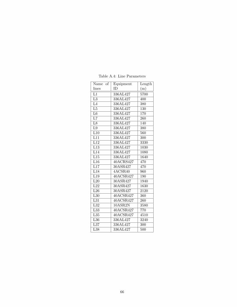
Table A.4: Line Parameters

Name oflines

EquipmentID

Length(m)

L1 336AL427 5700

L3 336AL427 400

L4 336AL427 380

L5 336AL427 130

L6 336AL427 170

L7 336AL427 260

L8 336AL427 140

L9 336AL427 380

L10 336AL427 560

L11 336AL427 300

L12 336AL427 3330

L13 336AL427 1030

L14 336AL427 1080

L15 336AL427 1640

L16 40ACRS427 470

L17 30ASR427 470

L18 4ACSR40 960

L19 40ACSR427 190

L20 30ASR427 1940

L22 30ASR427 1630

L26 30ASR427 2120

L30 40ACSR427 360L31 40ACSR427 260

L32 10ASR2N 3580

L33 40ACSR427 770

L35 40ACSR427 4510

L36 336AL427 3240

L37 336AL427 300

L38 336AL427 500

66

Tab

leA

.5:

NR

CA

NO

verh

ead

Lin

eP

ara

met

ers

Equ

ipm

ent

IDR

1(o

hm

s/km

)X

1(o

hm

s/km

)G

1(u

S/km

)B

1(u

S/km

)R

0(u

S/km

)X

0(o

hm

s/km

)G

0(u

S/km

)B

0(u

S/km

)

Su

mm

erR

ati

ng

(Am

ps)

Win

ter

Rati

ng

(Am

ps)

10A

SR

2N0.

5356

0.53

430

3.6

30.9

45

1.5

081

01.9

1301

301

336A

L42

70.

1696

0.38

090

4.3

30.4

689

1.2

808

01.9

655

655

30A

SR

427

0.34

80.

468

03.7

60.7

02

1.3

22

00

100

100

10A

SR

427

0.55

230.

4852

03.6

0.9

644

1.4

61

01.9

2321

321

40A

CS

R42

70.

2697

0.49

780

3.7

80.6

055

1.3

405

02.0

1452

452

4AC

SR

401.

3515

0.53

590

3.3

61.7

817

1.6

524

01.8

2172

172

67

Bibliography

[1] Ackermann, Thomas, Gran Andersson, and Lennart Sder. ”Distributed generation: a definition.”

Electric power systems research 57, no. 3 (2001): 195-204.

[2] Purchala, K., R. Belmans, L. Exarchakos, and A. D. Hawkes. ”Distributed generation and the grid

integration issues.” KULeuven, Imperial College London(2006).

[3] Bloemink, Jeffrey Michael. Validation of a Novel Approach to Voltage Sourced Converter Control

for MicroGrid Applications. ProQuest, 2007.

[4] Midtsund, Tarjei. ”Control of Power Electronic Converters in Distributed Power Generation Sys-

tems: Evaluation of Current Control Structures for Voltage Source Converters operating under

Weak Grid Conditions.” (2010).

[5] Kouro, Samir, Jose Leon, Dimitri Vinnikov, and Leopoldo G. Franquelo. ”Grid-Connected Pho-

tovoltaic Systems: An Overview of Recent Research and Emerging PV Converter Technology.”

Industrial Electronics Magazine, IEEE 9, no. 1 (2015): 47-61.

[6] Hassaine, L., E. OLias, J. Quintero, and V. Salas. ”Overview of power inverter topologies and control

structures for grid connected photovoltaic systems.”Renewable and Sustainable Energy Reviews 30

(2014): 796-807.

[7] Reed, Gregory, Ronald Pape, and Masatoshi Takeda. ”Advantages of voltage sourced converter

(VSC) based design concepts for FACTS and HVDC-link applications.” In Power Engineering So-

ciety General Meeting, 2003, IEEE, vol. 3. IEEE, 2003.

[8] Yazdani, Amirnaser, and Reza Iravani. Voltage-sourced converters in power systems: modeling,

control, and applications. John Wiley and Sons, 2010.

[9] Fortescue, Charles L. ”Method of symmetrical co-ordinates applied to the solution of polyphase

networks.” American Institute of Electrical Engineers, Transactions of the 37, no. 2 (1918): 1027-

1140.

[10] Gellings, Clark W. ”Power to the People.” Power and Energy Magazine, IEEE9, no. 5 (2011): 52-63.

[11] Chiniforoosh, S., J. Jatskevich, A. Yazdani, V. Sood, V. Dinavahi, J. A. Martinez, and A. Ramirez.

”Definitions and applications of dynamic average models for analysis of power systems.” Power

Delivery, IEEE Transactions on 25, no. 4 (2010): 2655-2669.

68

[12] Mirhosseini, Mitra, Josep Pou, Baburaj Karanayil, and Vassilios Georgios Agelidis. ”Positive-and

negative-sequence control of grid-connected photovoltaic systems under unbalanced voltage condi-

tions.” In Power Engineering Conference (AUPEC), 2013 Australasian Universities, pp. 1-6. IEEE,

2013.

[13] Song, Hong-seok, and Kwanghee Nam. ”Dual current control scheme for PWM converter under

unbalanced input voltage conditions.” Industrial Electronics, IEEE Transactions on 46, no. 5 (1999):

953-959.

[14] Zhao, Junhui, Caisheng Wang, Bo Zhao, Feng Lin, Quan Zhou, and Yang Wang. ”A review of active

management for distribution networks: current status and future development trends.” Electric

Power Components and Systems 42, no. 3-4 (2014): 280-293.

[15] Abdel-Galil, T. K., A. E. B. Abu-Elanien, E. F. El-Saadany, A. Girgis, Y. A. R. I. Mohamed, M. M.

A. Salama, and H. H. M. Zeineldin. ”Protection coordination planning with distributed generation.”

Qualsys Engco. Inc (2007).

[16] Chan, F.C. ”Electrical Power Distribution Systems”(PDF). www.eolss.net.

[17] Graovac, Milan, Xiaolin Wang, Reza Iravani, and Chad Abbey. Integration of Storage in Electrical

Distribution Systems and its Impact on the Depth of Penetration of DG. Technical Report CETC

Number 2009-174/2009-10-21, Department of Electrical and Computer Engineering, University of

Toronto, Prepared for: Chad Abbey, Natural Resources Canada, CANMET Energy Technology

Centre, Quebec, May, 2008.

[18] Safigianni, Anastasia S., George N. Koutroumpezis, and Anastasios I. Spyridopoulos. ”Distributed

Generation Effects on Large-Scale Distribution Networks.” Engineering 6, no. 01 (2014): 34.

[19] IEEE Std 1159 2009 IEEE Recommended Practice for Monitoring Electric Power Quality. 26 June

2009

[20] Lehn, Peter W. ”Direct harmonic analysis of the voltage source converter.” Power Delivery, IEEE

Transactions on 18, no. 3 (2003): 1034-1042.

[21] Yazdani, Amirnaser. Modelling and Control of the Three-level Neutral Point Diode Clamped (NPC)

Converter for High-power Applications. University of Toronto, 2005.

[22] Dugan, Roger C., Mark F. McGranaghan, and H. Wayne Beaty. ”Electrical power systems quality.”

New York, NY: McGraw-Hill,— c1996 1 (1996).

[23] Chen, K., L. W. Montgomery, G. Klempner, J. Yagielski, J. Amos, M. Brimsek, and M. Sedlak.

”Comparing IEEE 50.13 and IEC 60034 standards for large cylindrical rotor synchronous machines.”

In Power and Energy Society General Meeting, 2010 IEEE, pp. 1-9. IEEE, 2010.

[24] Stevenson, William D. Elements of power system analysis. Vol. 196, no. 2. New York: McGraw-Hill,

1982.

[25] Grainger, John J., and William D. Stevenson. Power system analysis. Vol. 31. New York: McGraw-

Hill, 1994.

69

[26] Reddy, S. Chandrashekhar, G. Saritha, and N. Vikas. ”Effect of distributed generation on distri-

bution systems during faults.” In Green Computing Communication and Electrical Engineering

(ICGCCEE), 2014 International Conference on, pp. 1-9. IEEE, 2014.

70

Documents

Performance Evaluation of The VSC-Interfaced Distributed ... · Performance Evaluation of The VSC-Interfaced Distributed Resource Models Gorken Gumustekin Master of Applied Science