Performance and degradation tests on high temperature ...projekter.aau.dk/projekter/files/77230363/Master_thesis...Performance and degradation tests on high temperature proton exchange

Performance and degradation tests on high

temperature proton exchange membrane fuel cells

(HT-PEMFCs)

Ionela Florentina Grigoras

Aalborg University

Department of Energy Technology

Hydrogen Technology and Fuel Cells

Aalborg, Denmark

June 2013

2

3

Title: Performance and degradation tests on HT-PEMFCs

Semester: 10th semester

Project period: 01/02/2013 – 04/06/2013

ECTS: 30

Supervisor: Samuel Simon Araya, Søren Knudsen Kær

Project group: Group 1010

_____________________________________

Ionela Florentina Grigoras

Copies: 3

Pages, total: 79

Appendix: 5

Supplements: No

By signing this document, each member of the group confirms that all group members have

participated in the project work, and thereby all members are collectively liable for the contents of

the report. Furthermore, all group members confirm that the report does not include plagiarism.

SYNOPSIS:

The current work investigates experimentally the

effects of methanol-water vapor mixture concentrations

in a H3PO4 doped PBI-based HT-PEM fuel cell. To isolate

the effects of methanol-water vapor mixture from the

whole reformate gas, the carbon dioxide and carbon

monoxide are excluded from the experimental matrix.

Two types of experiments are conducted: performance

tests and degradation tests. The performance tests are

realized in order to study the effect of temperature and

the different vapor mixture concentrations on the fuel

cell. The effect of startup-shutdown cycles is studied

during the degradation tests.

The analysis of these effects is made based on the

impedance spectra measurements, polarization curves

and cyclic voltammetry measurements.

4

5

Abstract

Methanol steam reforming process can be a good solution for hydrogen generation in the case of

fuel cells. The use of hydrogen generated by such process to fuel a fuel cell can eliminate the issues

related to infrastructure and storage. But the hydrogen obtained through methanol steam reforming is

not pure, containing impurities such as carbon dioxide, carbon monoxide, water vapor and unconverted

methanol. Researches have been conducted on HT-PEM fuel cells to study the effects of fuel impurities.

The current work investigates experimentally the effects of methanol-water vapor mixture

concentrations in a H3PO4 doped PBI-based HT-PEM fuel cell. To isolate the effects of methanol-water

vapor mixture from the whole reformate gas, the carbon dioxide and carbon monoxide are excluded

from the experimental matrix. Two types of experiments are conducted: performance tests and

degradation tests. The performance tests are realized in order to study the effect of temperature and

the different vapor mixture concentrations on the fuel cell. The effect of startup-shutdown cycles is

studied during the degradation tests.

The analysis of these effects is made based on the impedance spectra measurements, polarization

curves and cyclic voltammetry measurements. The results showed that temperature and methanol-

water vapor mixture variations have an effect on the fuel cell performance. The increase in temperature

increases the cathode catalyst active area and decreases the charge transfer resistance. Methanol-water

vapor variations have an effect on the membrane conductivity when the cell is operated for longer times

and cause a decrease in the catalyst active area of the cathode.

During the startup/shutdown cycles performed with pure hydrogen the total voltage decay was of -

46.3 mV, while the degradation rate for the case with methanol at a concentration of 3% was of -7.9

mV/h.

6

Acknowledgments

I would like to express my gratitude to Samuel Simon Araya, my study supervisor, for its patient

guidance and useful critiques of this work. I am also thankful to my co-supervisor Professor Søren

Knudsen Kær for all the help during my master program at Aalborg University.

At the same time, I am grateful to my colleague Fan Zhou for his assistance in the laboratory and his

support to my project.

Aalborg, June 2013 Ionela F. Grigoras

7

Outline

This report consists of 5 chapters and presents the experimental study conducted on a H3PO4 doped

PBI-based HT-PEM fuel cell aimed to describe the effects of methanol-water vapor mixture and

startup/shutdown cycles on the performance and degradation of the cell.

Chapter 1 gives an introduction to fuel cells fundamentals, classification and hydrogen generation

methods that exist currently on the market. In this part the objectives of the current work are also

described.

Chapter 2 outlines the working principle of a high temperature PEM fuel cell used in the present

study, together with the main degradation modes and characterization techniques.

Chapter 3 presents the methodology for the work. In this section a brief description of the unit

assembly, test station and MEAs characteristics is given. The experimental procedure used during the

two types of experiments conducted in this study in also highlighted, followed by the measurement

techniques used for the characterization of the fuel cell performance and degradation.

Chapter 4 is divided in two sections and summarizes the results obtained from the different tests.

The two sections analyze the effects of methanol slip and temperature for the performance test and the

effect of startup/shutdown cycles for the degradation experiments.

Chapter 5 gives the final remarks and the future work that can be conducted in order to improve the

HT-PEM fuel cells characterization.

8

Contents

Abstract ......................................................................................................................................................... 5

Acknowledgments ......................................................................................................................................... 6

Outline .......................................................................................................................................................... 7

List of Figures .............................................................................................................................................. 10

List of tables ................................................................................................................................................ 13

Nomenclature ............................................................................................................................................. 14

1 Introduction ............................................................................................................................................. 17

1.1 Why fuel cells? .................................................................................................................................. 20

1.2 Hydrogen generation ........................................................................................................................ 21

1.2 Fuel Cell Fundamentals ..................................................................................................................... 24

1.3 Classification of fuel cells .................................................................................................................. 25

1.4 Objectives and limitations ................................................................................................................ 28

2 High Temperature PEM fuel cells ............................................................................................................. 29

2.1 Background ....................................................................................................................................... 29

2.2 Fundamentals of HT-PEMFC ............................................................................................................. 30

2.3 Degradation of HT-PEMFC ................................................................................................................ 32

2.4 HT-PEMFC characterization techniques ............................................................................................ 34

3 Methodology ............................................................................................................................................ 39

3.1 Description of the test set-up ........................................................................................................... 39

3.2 Experimental procedure ................................................................................................................... 42

3.2.1 Polarization curve – measurement technique ........................................................................... 45

3.2.2 Impedance spectra – measurement technique and analysis .................................................... 46

3.2.3 Cyclic voltammetry – measurement technique and analysis .................................................... 47

4 Results & Interpretation .......................................................................................................................... 49

4.1 Performance tests ............................................................................................................................. 49

4.1.1 Effect of operating temperature ................................................................................................ 49

4.1.2 Effect of methanol slip ............................................................................................................... 57

4.2 Degradation tests .............................................................................................................................. 61

9

4.2.1 H2 continuous test ...................................................................................................................... 64

4.2.2 H2 startup/shutdown test .......................................................................................................... 65

4.2.3 Methanol continuous test .......................................................................................................... 66

4.2.4 Methanol startup/shutdown test .............................................................................................. 67

5 Conclusion & Future work........................................................................................................................ 69

5.1 Final remarks ..................................................................................................................................... 69

5.2 Future work ....................................................................................................................................... 70

6 References ............................................................................................................................................... 71

Appendix A – Matlab script ......................................................................................................................... 75

Appendix B – HyAL script for EIS measurements ........................................................................................ 76

Appendix C – HyAL script for polarization curves ....................................................................................... 77

Appendix D – Fitted resistances for each performance experiment .......................................................... 78

10

List of Figures

Figure 1 World CO2 emissions from 1971 to 2010 by region (Mt of CO2), source [5]; Asia*** = Asia

excluding China ........................................................................................................................................... 17

Figure 2 World CO2 emissions from 1971 to 2010 by fuel (Mt of CO2), source [5] .................................... 18

Figure 3 IPCC CO2 emission scenarios, source [9] ....................................................................................... 18

Figure 4 Alternative World Energy Outlook, reproduced from [10] ........................................................... 19

Figure 5 Working principle of a PEM-based electrolyzer, adapted from [18] ............................................ 21

Figure 6 Basic working principle of a fuel cell ............................................................................................. 25

Figure 7 Working principle of a PEM fuel cell, source [18] ......................................................................... 30

Figure 8 Parts of a HT-PEMFC single cell, source [30] ................................................................................. 31

Figure 9 Chemical structure of PBI repeat unit, source [22] ....................................................................... 32

Figure 10 Polarization curve of a PEM fuel cell with the various loss-regions, source [37] ....................... 34

Figure 11 Nyquist plot, source [22] ............................................................................................................. 35

Figure 12 Current vs. time........................................................................................................................... 37

Figure 13 Cyclic voltammogram, source [41].............................................................................................. 37

Figure 14 Flow fields design ........................................................................................................................ 40

Figure 15 Schematic of the test set-up ....................................................................................................... 41

Figure 16 Fuel cell picture ........................................................................................................................... 42

Figure 17 Equivalent circuit model ............................................................................................................. 46

Figure 18 Fitting between impedance experimental data and the resulting impedance of the equivalent

circuit .......................................................................................................................................................... 46

Figure 19 Specifications of the equivalent circuit model ............................................................................ 48

Figure 20 Polarization curve of no-preheat hydrogen performance tests ................................................. 50

Figure 21 Polarization curve of preheat hydrogen performance tests ....................................................... 50

Figure 22 EIS spectra for no-preheat hydrogen performance test ............................................................. 50

Figure 23 EIS spectra for preheat hydrogen performance test .................................................................. 50

Figure 24 Polarization curve of 100% conversion performance tests ........................................................ 51

Figure 25 Polarization curve of 98% conversion performance tests .......................................................... 51





Figure 30 Ohmic resistances for room temperature and preheat hydrogen experiments ........................ 52

Figure 31 Ohmic resistances for performance experiments conducted with different concentrations of

methanol-water vapor mixture .................................................................................................................. 52

Figure 32 High frequency resistances for room temperature and preheat hydrogen experiments .......... 52

Figure 33 High-frequency resistances for performance experiments conducted with different

concentrations of methanol-water vapor mixture ..................................................................................... 52

Figure 34 Low frequency resistances for room temperature and preheat hydrogen experiments ........... 53

11

Figure 35 Low-frequency resistances for performance experiments conducted with different

concentrations of methanol-water vapor mixture ..................................................................................... 53

Figure 37 EIS spectra for 100% conversion performance test .................................................................... 53

Figure 38 EIS spectra for 98% conversion performance test ...................................................................... 53





Figure 42 Cyclic voltammogram of performance tests at ........................................................................... 56


Figure 44 Cyclic voltammogram of performance tests at 160 oC ............................................................... 56



Figure 47 Polarization curve of performance tests conducted with different vapor mixture

concentrations at a constant temperature of 160 oC ................................................................................. 57

Figure 48 EIS spectra for performance tests conducted with different vapor mixture concentrations at a

constant temperature of 160 oC ................................................................................................................. 58

Figure 49 Fitted resistances for performance tests conducted with different vapor mixture

concentrations at a constant temperature of 160 oC ................................................................................. 58

Figure 50 Cyclic voltammogram of 100% conversion performance tests for different temperatures ...... 59

Figure 51 Cyclic voltammogram of 98% conversion performance tests for different temperatures ........ 59





Figure 56 Polarization curves for durability test with MeOH ..................................................................... 60

Figure 57 EIS spectra for durability test with MeOH .................................................................................. 60

Figure 58 Fitted resistances for durability test with MeOH........................................................................ 60

Figure 59 Polarization curve for the break-in test of 1st Danish Power System MEA ................................. 62

Figure 60 Polarization curve for the break-in test of 2nd Danish Power System MEA ................................ 62

Figure 61 EIS spectra for break-in ............................................................................................................... 62

Figure 62 Break-in fitted resistances .......................................................................................................... 62

Figure 63 Voltage profile for the 1st MEA .................................................................................................. 63

Figure 64 Voltage profile for the 2nd MEA ................................................................................................. 63

Figure 65 Polarization curve for the hydrogen continuous test of the 1st Danish Power System MEA ..... 64

Figure 66 Polarization curve for the hydrogen continuous test of the 2nd Danish Power System MEA ..... 64

Figure 67 Voltage profile of the hydrogen continuous test ........................................................................ 64

Figure 68 Fitted resistances for H2 continuous test ................................................................................... 64

Figure 69 Voltage profile of the hydrogen startup/shutdown test ............................................................ 65

Figure 70 Polarization curve for the hydrogen startup/shutdown test of the 1st Danish Power System

MEA ............................................................................................................................................................. 65

Figure 71 Fitted resistances for H2 startup/shutdown test ........................................................................ 66

12

Figure 72 Voltage profile of the methanol continuous test ....................................................................... 66

Figure 73 Polarization curve for the methanol continuous test on the 1st Danish Power System MEA .... 66

Figure 74 Fitted resistances for MeOH continuous test ............................................................................. 67

Figure 75 Voltage profile of the methanol startup/shutdown test ............................................................ 68

Figure 76 Polarization curve for the MeOH start/stop test of the 2nd Danish Power System MEA ........... 68

Figure 77 Pure Hydrogen fitted resistances ................................................................................................ 78

Figure 78 Preheat Hydrogen fitted resistances .......................................................................................... 78

Figure 79 100% conversion fitted resistances ............................................................................................ 78

Figure 80 98% conversion fitted resistances .............................................................................................. 78





13

List of tables

Table 1 Classification of relevant fuel cell types, adapted from [22] ......................................................... 26

Table 2 The various types of fuel cells and the electrode reactions, adapted from [47] ........................... 26

Table 3 Circuits elements used in the EC models, adapted from [39] ........................................................ 36

Table 4 Details of tested single cell ............................................................................................................. 39

Table 5 Details of the fuel cell components................................................................................................ 40

Table 6 Specifics of the MEA components .................................................................................................. 40

Table 7 Operating conditions and inputs of the performance tests conducted at 140 oC ......................... 44

Table 8 Operating condition and inputs of the degradation tests ............................................................. 45

Table 9 Hydrogen desorption charge (mC) ................................................................................................. 55

Table 10 Estimated cathode catalyst active area (cm2) .............................................................................. 55

14

Nomenclature

Acronyms

AC Alternating Current AFC Alkaline Fuel Cell C Capacitor CL Catalyst Layer CNLS Complex Non-linear Least Square CV Cyclic Voltammetry CPE Constant Phase Element CHP Combined of Heat and Power DC Direct Current DMFC Direct Methanol Fuel Cell EC Equivalent Circuit EIS Electrochemical Impedance Spectroscopy F Faraday’s constant GDL Gas Diffusion Layer GHG Greenhouse Gas HT-PEMFC High Temperature Proton Exchange Membrane Fuel Cell ICE Internal Combustion Engine IPCC Intergovernmental Panel on Climate Change I Current L Inductor MCFC Molten Carbonate Fuel Cell MEA Membrane Electrode Assembly OECD Organization for Economic Co-operation and Development ORR Oxygen Reduction Reaction n Number of electrons PBI Polybenzimidazole PAFC Phosphoric Acid Fuel Cell PEM Proton Exchange Membrane PEMFC Proton Exchange Membrane Fuel Cell PV Photovoltaic Psat Saturation pressure PH2O Pressure of water RH Relative Humidity R Resistor Rhf High frequency resistance Rlf Low frequency resistance Rohmic Ohmic resistance SOFC Solid Oxide Fuel Cell T Temperature Tgas Gas temperature Tdew_point Dew point temperature V Voltage

15

VH2 Volume flow rate of hydrogen Vair Volume flow rate of air Z Impedance WGS Water Gas Shift Phase angle Frequency Stoichiometry

Hydrogen stoichiometry

Air stoichiometry

16

17

1 Introduction

Different and serious problems are affecting the world currently, starting from natural resources

depletion, to global warming, environmental destruction and over-population. These problems are the

consequence of different factors such as economic development, resource intensive lifestyle of people

from developed countries and the increasing degree of urbanization [1].

According to the estimations of the International Energy Outlook from 2011 [2], the world energy

demand is about 400 EJ per year and approximately 80 % of this energy demand is derived from fossil

fuels. The same source [2] predicts that the world energy demand will continue to increase in the future,

for example for 2030 the value is expected to reach about 700 EJ.

The CO2 emissions are also expected to rise by 43 % until 2035 [2]. This way, the greenhouse gas

(GHG) emissions will not be reduced by 50 – 85 % by 2050, a condition necessary for maintaining global

warming below 2 oC and avoiding climate change [3]. In 2011 global emissions of carbon dioxide grew by

3.2 % [3], the emissions obtained from fossil fuels combustion reaching a value of 31.6 Gt [4]. Figure 1

presents the global carbon dioxide emissions by region over a period of almost 40 years, which shows

clearly that along the years CO2 emissions have increased in developing countries such as China and

some other countries of Asia, while the OECD countries have kept their emissions almost constant.

Figure 1 World CO2 emissions from 1971 to 2010 by region (Mt of CO2), source [5]; Asia*** =

Asia excluding China

China is a leader in emitting pollutants into atmosphere. In 2011, China had a share of 28% of the

global emissions, being followed by the United States (16%), the European Union (11%) and India (7%)

[3]. Figure 2 shows the world CO2 emissions by fuel from 1971 to 2010. It can be noticed that CO2

emissions coming from burning coal, oil or natural gas have been increasing over the time, in 2011 these

emissions accounted for 45 % in the case of coal, 35 % for oil and 20 % for natural gas respectively [4].

18

Figure 2 World CO2 emissions from 1971 to 2010 by fuel (Mt of CO2), source [5]

Since most of the world energy is derived from fossil fuels, the oil production capacity is questioned

all the time, the global oil reserves accounting for almost 1652.6 billion barrels in 2011 [6]. Oil is an

exhaustible resource. Its prices have been increasing since 1970s, exceeding $118 in February 2013 [7].

Nowadays, approximately 90 million barrels per day of oil are being consumed worldwide [7]. This

consumption of conventional fuels has led the atmospheric CO2 concentrations to reach critical values,

such as the ones presented by different scenarios reported by IPCC in Figure 3.

Figure 3 IPCC CO2 emission scenarios, source [9]

There is no doubt that the world energy still relies mainly on fossil fuels and at one moment in the

future these non-renewable resources will be depleted taking into consideration the world energy

300

400

500

600

700

800

900

CO

2 co

nce

ntr

atio

n (

pp

m)

Year

CO2 emission scenarios

Scenario A1B

Scenario A2

Scenario B1

19

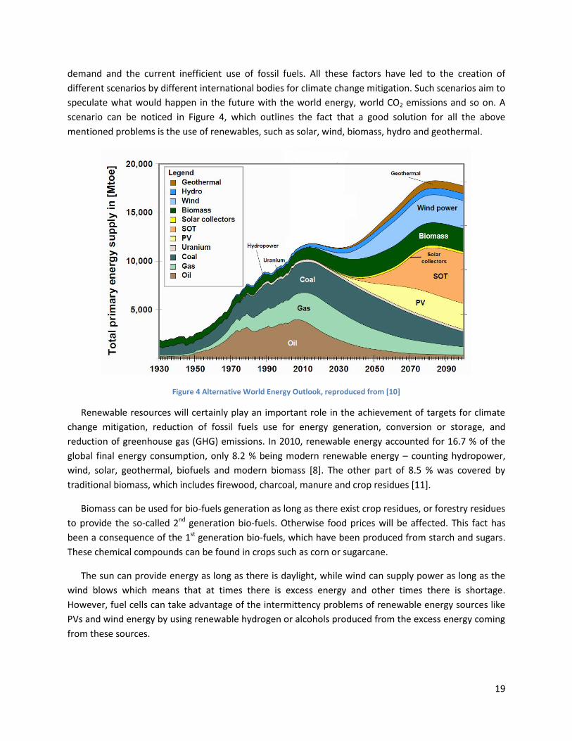
demand and the current inefficient use of fossil fuels. All these factors have led to the creation of

different scenarios by different international bodies for climate change mitigation. Such scenarios aim to

speculate what would happen in the future with the world energy, world CO2 emissions and so on. A

scenario can be noticed in Figure 4, which outlines the fact that a good solution for all the above

mentioned problems is the use of renewables, such as solar, wind, biomass, hydro and geothermal.

Figure 4 Alternative World Energy Outlook, reproduced from [10]

Renewable resources will certainly play an important role in the achievement of targets for climate

change mitigation, reduction of fossil fuels use for energy generation, conversion or storage, and

reduction of greenhouse gas (GHG) emissions. In 2010, renewable energy accounted for 16.7 % of the

global final energy consumption, only 8.2 % being modern renewable energy – counting hydropower,

wind, solar, geothermal, biofuels and modern biomass [8]. The other part of 8.5 % was covered by

traditional biomass, which includes firewood, charcoal, manure and crop residues [11].

Biomass can be used for bio-fuels generation as long as there exist crop residues, or forestry residues

to provide the so-called 2nd generation bio-fuels. Otherwise food prices will be affected. This fact has

been a consequence of the 1st generation bio-fuels, which have been produced from starch and sugars.

These chemical compounds can be found in crops such as corn or sugarcane.

The sun can provide energy as long as there is daylight, while wind can supply power as long as the

wind blows which means that at times there is excess energy and other times there is shortage.

However, fuel cells can take advantage of the intermittency problems of renewable energy sources like

PVs and wind energy by using renewable hydrogen or alcohols produced from the excess energy coming

from these sources.

20

1.1 Why fuel cells?

Fuel cells are an old technology that hasn’t reached maturity yet. They were invented for the first

time in 1839 by Sir William Grove, who believed that electricity and water could be obtained by

reversing the electrolysis procedure [12]. He proved his hypothesis and called the first fuel cell – gas

voltaic battery. Since 1932, when the first fuel cell application was demonstrated, research has been

done in this area in order to develop more performing and durable fuel cells [12].

Fuel cells have been used in a variety of applications, starting from electronic equipment such as

portable computers (20 – 50 W), mobile phones or military communication equipment, to vehicles (50 –

125 kW), stationary applications like backup powers, combined heat and power systems for residential

households (1 – 5 kW) and commercial buildings, central power generation (1 – 200 MW or more), space

craft etc. [13].

Recently, transportation has been using a large part of the fossil fuels and has a huge contribution to

the greenhouse gas emissions. The world population growth has led to an increase in transportation

use. This issue has raised the demand for cleaner vehicles.

A fuel cell-powered car has an overall efficiency of about 64 %, if the fuel cell uses pure hydrogen,

compared to a gasoline-powered car, whose efficiency is very low, only 20 % [14]. As an example, the

overall efficiency for the Honda’s FCX concept vehicle was reported to be 60 % [14]. This efficiency

reduces if the fuel source is not pure hydrogen. In contrast, battery-powered electric cars have the

highest efficiency – 72 %. But this efficiency can drop to 26% if the entire cycle of generating the

electricity necessary to power the car is considered. However, the overall efficiency can reach 65 % if the

electricity is generated by a renewable resource [14].

The cost of such a fuel cell used to power a car has been reduced over time according to the U.S.

Department of Energy. Its value in 2002 was of about $275/kW and decreased along time to a value of

$49/kW in 2011, if a volume production of 500 000 units per year is assumed [15]. In order to compete

with the current technology of Internal Combustion Engines (ICEs), which costs around $25 – $35/kW,

the cost per kW for an automotive fuel cell has to continue decreasing [15].

Fuel cells can also be 100 % CO2 neutral if the hydrogen is derived from renewable energy sources,

the only by-products of the main fuel cell reaction being pure water and heat [16]. Other important

characteristics of fuel cells are that they have very few moving parts, which make them to operate

quietly, and they are flexible in terms of fuels [16]. Besides that, fuel cells can also contribute to the

reduction of some of the problems associated with energy production from fossil fuels, such as air

pollution, GHG emissions and economic dependence of oil [16].

However, there are some problems that prevent fuel cells from large scale commercialization. These

problems are related to cost, which continues to be high due to fuel cell components. For example in

the case of PEM fuel cells, the catalyst used (Platinum), gas diffusion layers and bipolar plates represent

21

approximately 70 % of the fuel cell total cost [13]. This is why research is ongoing to decrease the

amount of catalyst needed or to thinner the bipolar plates. Other disadvantages of fuel cells are

hydrogen generation, delivery infrastructure, storage considerations and safety issues [14].

1.2 Hydrogen generation

Hydrogen is the lightest element in the periodic table and has the highest energy content per unit

mass of all the fuels, its higher heating value being 141.9 MJ/kg [17]. Although it is the most abundant

element in the universe, it has to be produced from sources such as hydrocarbons or water. There are

different ways of producing hydrogen from water, including: electrolysis, photolysis, photo-

electrochemical processes and photo-catalysis [18].

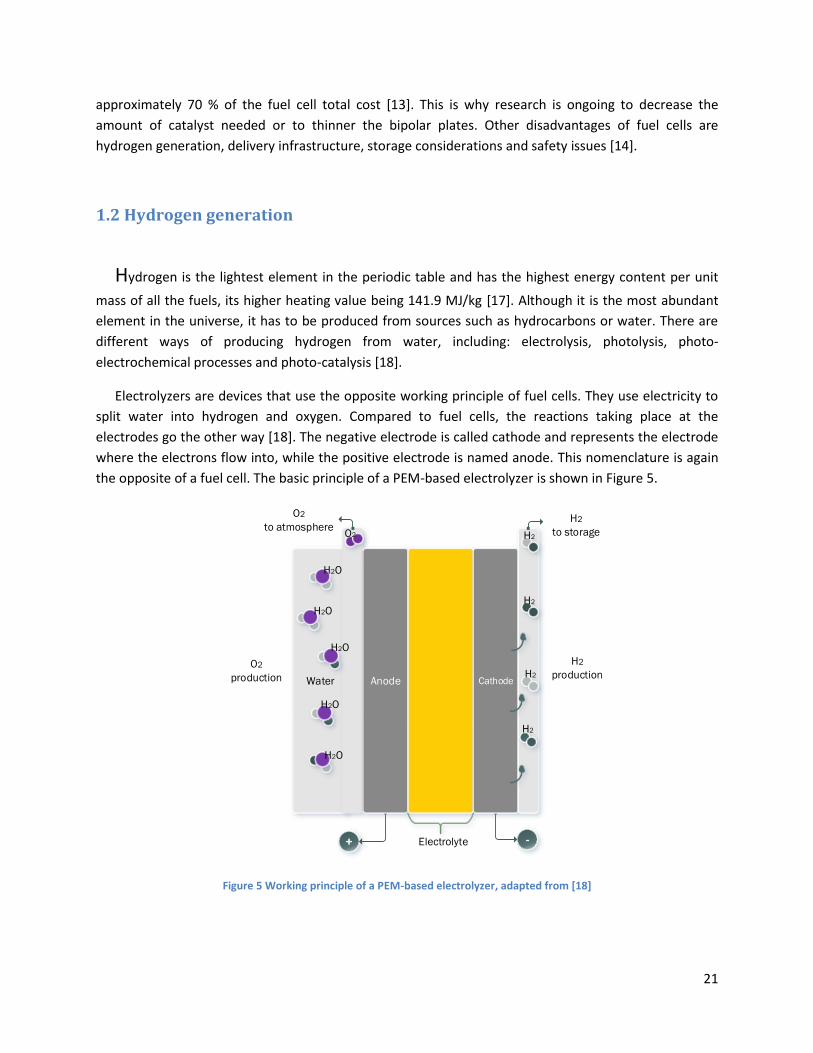
Electrolyzers are devices that use the opposite working principle of fuel cells. They use electricity to

split water into hydrogen and oxygen. Compared to fuel cells, the reactions taking place at the

electrodes go the other way [18]. The negative electrode is called cathode and represents the electrode

where the electrons flow into, while the positive electrode is named anode. This nomenclature is again

the opposite of a fuel cell. The basic principle of a PEM-based electrolyzer is shown in Figure 5.

+ -Electrolyte

H2

productionO2

production Water

H2O

H2O

H2O

H2O

H2O

O2

Anode Cathode

H2

H2

H2

H2

O2

to atmosphereH2

to storage

Figure 5 Working principle of a PEM-based electrolyzer, adapted from [18]

22

Electrolyzers offer the advantage of producing high purity hydrogen when is needed and much

cheaper, eliminating this way the necessity of storing the hydrogen or supplying it in high pressure

cylinders [18].

The reactions by which hydrogen and oxygen are formed are represented in the following chemical

formulae:

Negative electrode (cathode): Eq. (1)

Positive electrode (anode): Eq. (2)

Hydrogen can also be generated by gasifying biomass, which results in a gas mixture composed

mainly of hydrogen and carbon monoxide. This mixture is usually called synthesis gas or syngas.

Gasification is a partial oxidation or steam reforming process taking place at high temperatures, typically

in the range of 800 – 900 oC [19]. Steam reforming of natural gas, bio-gas or bio-oil is an endothermic

process which leads to synthesis gas. The steam reforming reaction equation can be described by the

following chemical formula [19]:

(

) Eq. (3)

For example, the equation for natural gas steam reforming is given in eq. (4).

Eq. (4)

The product of the steam reforming reaction is called reformate and contains significant amounts of

unconverted steam and to a lesser extent unconverted fuel. Steam reforming is a challenging

technology, many problems occurs during the process such as coke formation, or side reactions

including water gas shift reaction (eq. (5)), Boudouard reaction (eq. (6)), CO reduction reaction (eq. (7))

or the methane decomposition reaction (eq. (8)) [20]. Carbon formation poisons the catalyst. The steam

to carbon ratio is also important during this process because the lower the steam content, the higher

the probability of carbon formation [19]. Usually, nickel-based catalysts are used in the steam reforming

process.

Eq. (5)

Eq. (6)

Eq. (7)

Eq. (8)

Methane steam reforming takes place at high temperatures of around 800 – 900 oC as already stated

above, but methanol is reformed at intermediate temperatures of around 250 – 300 oC [29]. Methanol

steam reforming reaction is given in equation 9.

23

Eq. (9)

Partial oxidation is a process taking place at temperatures between 1200 – 1500 oC. Compared to

steam reforming process, which requires the presence of a catalyst, in this case at such high

temperatures, the catalyst is not needed [18, 19]. Another advantage of this process is that fuels do not

require sulfur removal [18, 19]. The reaction of methane partial oxidation is:

Eq. (10)

A combination of the steam reforming and partial oxidation processes is called auto-thermal

reforming and describes a process in which both steam and oxidant are fed with the fuel to a catalytic

reactor [18].

The carbon monoxide resulting from the reforming processes can be converted into other gases that

act as diluents when they are present in the fuel steam of a fuel cell [18]. There are three ways of

removing the carbon monoxide from the fuel stream of a fuel cell: selective oxidation, methanation and

the use of palladium/platinum membranes. In a selective oxidation reactor, a small amount of air is

added to the fuel stream and passed over a precious metal catalyst. The catalyst absorbs the CO where

it reacts with the oxygen in the air. However, this method is dangerous due to the presence of hydrogen,

oxygen and carbon monoxide which is an explosive mixture [18]. Methanation is an alternative to the

danger of producing explosive gas mixtures, the reaction being described in eq. (11).

Eq. (11)

Methane does not poison the fuel cell, by acting as a diluent, but this method is disadvantageous due

to the use of too much hydrogen. Hydrogen generated by steam reforming can also be purified using

palladium/platinum membranes, but the cost of these membranes is a drawback [18].

There are also some biological methods of producing hydrogen which involves the use of bacteria or

microorganisms. Anaerobic digestion is a biochemical process that uses bacteria to break down the

organic matter from biomass. The process takes place in the absence of oxygen and produces biogas,

which is a mixture of methane, carbon dioxide and traces of hydrogen, carbon monoxide, nitrogen and

hydrogen sulfide [21]. Bio-photolysis produces hydrogen from algae in the presence of water and

sunlight [17].

Methanol is the preferred fuel as the long term option for steam reforming. Ref. [18] listed some

developers of methanol reforming for vehicles in 2003, among which Daimler Chrysler, General Motors,

Honda, Mitsubishi, Nissan, Toyota. For example the General Motors methanol processor for the Zafira

concept car in 1998 had an energy efficiency of 82 – 85 % and a methanol conversion of 99 % [18]. The

maximum unit size was of 30 kWe and the power density was of 0.5 kWe/L [18].

There are different methods of storing hydrogen, among which one can count [17, 18]: compression

in gas cylinders, storage as cryogenic liquid, storage in a metal absorber (metal hydrides) and storage in

carbon nano-fibers.

24

Being the smallest molecule on Earth, hydrogen has the tendency to escape through small openings,

holes or joints of low pressure pipelines. The hydrogen leak from these pipelines is much faster than a

natural gas leak [17]. In mixture with air, hydrogen has a lower flammability limit, which is much higher

than that of propane or gasoline, and slightly lower than that of natural gas [17]. The lower flammability

limit of a fuel determines if the fuel leak would ignite. But if it does ignite, hydrogen is very dangerous

due to the fact that hydrogen flame is nearly invisible [17].

1.2 Fuel Cell Fundamentals

A fuel cell is an electrochemical device that directly converts chemical energy from hydrogen-rich

fuels into electricity, with pure water and heat as the only by-products. Since the only exhaust of the

process are heat and water, fuel cells are one of the cleanest technologies that are available on the

market when they are fed with pure hydrogen and oxygen, and the hydrogen is derived from renewable

resources [22]. The voltage output of a single cell is in the range of 0.6 – 0.8 V, this value is barely

enough even for the smallest application. That is why individual cells are usually connected in series in

order to increase the voltage; this arrangement forms a fuel cell stack, whose overall voltage is the sum

of all the individual cells. Moreover, the power produced by a fuel cell depends on some important

factors, which include the fuel cell type, size, the temperature at which it operates and pressure at

which gasses are supplied [13]. As already discussed, there are two fundamental technical problems

with fuel cells if the manufacturing and materials costs are not considered [13, 18]:

(1) slow reaction rate which leads to low currents and power, but this problem can be overcome by

using catalysts such as Platinum, by increasing the temperature or the electrode area (using

highly porous electrodes);

(2) hydrogen, which has raised concerns about its generation, delivery infrastructure, storage and

safety.

The three main components of a fuel cell are: the anode (fuel electrode), cathode (oxidant electrode)

and the electrolyte which is sandwiched between them. These components form the so-called

membrane electrolyte assembly (MEA). A basic principle of a fuel cell can be seen in Figure 6.

At the anode, hydrogen is oxidized into protons (H+) and electrons (e-). The membrane electrolyte

allows only the protons to migrate through it, while the electrons are transferred through an external

circuit to the cathode, generating electricity in the same time. At the cathode, the protons and electrons

will react with oxygen to form water.

The anode reaction is: Eq. (12)

The cathode reaction is:

Eq. (13)

25

H2

H2

H2

H2

H2

H2 inlet

Excess H2

ANODE CATHODEMembrane

Electrolyte

O2

O2

O2

H2O

e- e-

e-

e-

e- H+

H+

H+

H+

H+

H+

H+

e-

e-

O2

H2O + Heat

O2 inlet

Figure 6 Basic working principle of a fuel cell

1.3 Classification of fuel cells

There are different types of fuel cells, and each type operates a bit differently and can say a lot

about the power produced by the respective fuel cell and the utilization of such a fuel cell. Fuel cells are

usually classified by the type of electrolyte used [14], which determines the kind of chemical reaction

that takes place in the fuel cell, and sometimes based on the temperature range of operation [13, 22].

Table 1 presents a classification of the relevant fuel cell types, while the specific electrode reactions can

be seen in Table 2.

There are advantages and drawbacks in each type of fuel cell. Cost is a common issue that affects all

the fuel cell types. Some disadvantages in the case of alkaline fuel cells are related to liquid electrolyte

management and electrolyte degradation [47]. Moreover, this type of fuel cell is very sensitive to the

carbon dioxide present into the atmosphere. The CO2 from air can be absorbed into the alkaline

electrolyte and form Potassium Carbonate (K2CO3), which can deposit on the cathode, fouling it [24].

26

Table 1 Classification of relevant fuel cell types, adapted from [22]

Fuel Cell Type

Electrolyte Operating temperature

Electrical efficiency

Typical electrical

power

Applications

PEMFC Ion exchange membrane (water based)

60 – 80 oC 40 – 60 % < 250 kW Vehicles, small stationary

HT-PEMFC Ion exchange membrane (acid base)

120 – 200 oC 60 % < 100 kW Small stationary

DMFC Polymer membrane 60 – 130 0C 40 % < 1 kW Portable MCFC Lithium/Potassium

carbonate 650 oC 45 – 60 % > 200 kW Stationary

PAFC Liquid phosphoric acid 200 oC 35 – 40 % > 50 kW Stationary SOFC Yttrium stabilized

zirconia 1000 oC 50 – 65 % < 200 kW Stationary

AFC Potassium hydroxide solution

60 – 90 oC 45 – 60 % > 20 kW Submarines, spacecraft

Table 2 The various types of fuel cells and the electrode reactions, adapted from [47]

Fuel cell type Electrode reactions

PEMFC Anode: Cathode:

DMFC Anode: Cathode:

AFC Anode: Cathode:

PAFC Anode: Cathode:

MCFC Anode: Cathode:

SOFC Anode: Cathode:

The high temperature in solid oxide fuel cells can cause the fuel cell parts to break down when it is

operated in start/stop cycles [14]. The high operating temperatures offer the advantage of using the

steam produced by the fuel cell in a co-generation of heat and power (CHP) process. The extra electricity

generated by channeling the steam into turbines improves the overall efficiency of the system from 50

% - 60 % to about 80 % - 85 % [48]. Another feature of these fuel cells is the ability of reforming fuels

internally, which reduces the cost associated with adding an external reformer to the system, and

increases the tolerance to sulfur and carbon monoxide [48]. Additional problems related to thermal

27

expansion and stability to mechanical damage have also to be considered when working with solid oxide

fuel cells [48]. Slow startups and thermal sealing are other drawbacks of the SOFCs [47].

As in the case of solid oxide fuel cells, the MCFCs can also take advantage of the high operating

temperatures by using the internal reforming process or by improving its efficiency using the waste heat

[48]. Although this type of fuel cell is more resistant to fuel impurities, the startup and thermal sealing

still remain an issue [24].

Most of the fuel cells are operating on pure hydrogen, but problems regarding storage of hydrogen

are still an issue to the technology development, as well as handling and safety issues. Methanol can be

used as alternative fuel because it is liquid and can be easily transported and stored within the current

network, and moreover it is cheaper than hydrogen [18]. Direct methanol fuel cells offer the advantage

of using methanol as anode feed gas.

Proton Exchange membrane (PEM) fuel cells are characterized by having a polymer membrane

proton conductor, as the name suggests which is sandwiched between the anode and the cathode.

These fuel cells operate at relatively low operating temperatures (Table 1) compared to solid oxide or

molten carbonate fuel cells and present a high power density [14]. Taking into account the low

operating temperatures, these fuel cells do not require long times to warm up and start generating

electricity [14].

The polymer membrane presents some advantages compared to liquid electrolytes, which includes

the easy handling, compactness, strength and elasticity at the same time [25]. Solid proton exchange

membranes are also amenable to mass production and can be fabricated into films of small thickness

still resistant to gases permeation [25]. These fuels cells are very sensitive to contaminants in the fuel

gas, especially to CO which must be reduced below 10 ppm in order to avoid deterioration in the anode

performance [24].

Using a solid proton exchange membrane instead of a liquid electrolyte in a fuel cell makes handling,

sealing and assembling much easier and the pressure imbalance tolerance between half-cells is as well

improved [25]. The problems associated with this kind of fuel cells are related to the low operating

temperatures, CO poison, and humidification of gaseous reactants [24, 25].

In order to overcome these challenges, high temperature PEM fuel cells (HT-PEMFCs) were

developed as a solution. HT-PEMFCs operate at temperatures in the range of 140 – 180 oC, some

manufacturers report a range of 120 – 200 oC. High temperature PEM fuel cells will be described in the

following chapter, where the major technological problems associated with this kind of fuel cells,

together with the characterization methods will also be outlined. The main objectives of this report will

be further presented.

28

1.4 Objectives and limitations

Methanol steam reforming process can be a good solution for hydrogen generation. This process

offers a variety of advantages compared to other technologies used currently in this scope. First of all,

methanol is a liquid fuel that can be easily transported and stored within the current network compared

to hydrogen. In the case of hydrogen, infrastructure and storage issues are the main barriers to the

technology development, as well as handling and safety issues. Secondly, methanol is much cheaper

than hydrogen. Besides all the methanol properties, the steam reforming process of methanol takes

place at temperatures between 250 oC and 300 oC, much lower than the natural gas steam reforming for

example, whose reforming temperature is around 800 – 900 oC. The lower temperature can reduce the

cost of materials used in the reforming process.

The use of hydrogen generated by such process to fuel a fuel cell can eliminate the issues related to

infrastructure and storage. But the hydrogen obtained through methanol steam reforming is not pure,

containing impurities such as carbon dioxide, carbon monoxide, water vapor and unconverted

methanol. Researches have been conducted on HT-PEM fuel cells to study the effect of fuel impurities,

and most of the studies have considered all the mentioned impurities in their experimental work. For a

better understanding of how a high temperature fuel cell is affected when is operated on reformate gas

used as anode feed gas, the effects of each impurity has to be study.

The current work investigates experimentally the effects of methanol-water vapor mixture

concentrations in a H3PO4 doped PBI-based HT-PEM fuel cell. To isolate the effects of methanol-water

vapor mixture from the whole reformate mixture, the carbon dioxide and carbon monoxide are

excluded from the experimental matrix. Two types of experiments are conducted: performance tests

and degradation tests. The performance tests are realized in order to study the effect of temperature

and the different vapor mixture concentrations on the fuel cell. The effect of startup-shutdown cycles is

studied during the degradation tests.

The analysis of these effects is made based on the impedance spectra measurements, polarization

curves and cyclic voltammetry measurements. Due to some problems encountered during experiments,

cyclic voltammetry measurements were realized only for the performance tests. The last part of

degradation tests does not present impedance spectra measurements.

29

2 High Temperature PEM fuel cells

This chapter presents the fundamentals of high temperature PEM fuels cells, more specifically of

phosphoric acid doped polybenzimidazole (PBI)-based high temperature PEM fuel cells, together with the

problems related to their technology and characterization techniques.

2.1 Background

As pointed out in the first chapter, proton exchange membrane or polymer electrolyte membrane

(PEM) fuel cells are classified as low-temperature fuel cells, operating at 60 – 80 oC and having a high

power density [14]. The electrolyte employed in such fuel cells is a solid polymer which presents

numerous advantages compared to liquid electrolytes. These fuel cells have an efficiency of 60 % when

they are used in transportation and of about 35 % for stationary applications such as backup power,

distributed generation or portable power [13]. Of the advantages of this type of fuel cell one can count

that the solid electrolyte reduces corrosion and the problems related to liquid electrolyte management,

the low operating temperatures give a quick start-up to the cell because it doesn’t need to warm up

very long before beginning to generate electricity [13, 14]. Besides these advantages, there are also

some challenges encountered in this type of fuel cell technology, which include the expensive catalyst,

the sensitivity to impurities and the low temperature waste heat [13].

Compared to low-temperature PEM fuel cells, or simply PEM fuel cells, high temperature PEM fuel

cells (HT-PEMFCs) have capture a lot of attention since their discovery in 1995 by Wang et al. [26]. This is

because of the fact that HT-PEM fuel cells are more tolerant to impurities due to the intermediate

operation temperature, more reliable in terms of improved reaction kinetics, heat rejection or water

management with respect to their low temperature counter parts [22, 25]. The tolerance to impurities

makes this type of fuel cells suitable to be fed with hydrogen obtained from reforming processes of

hydrocarbons or alcohols such as natural gas, gasoline or methanol. The use of hydrogen obtained

through reforming processes eliminates the different problems related to hydrogen storage or the need

for a new infrastructure to distribute and supply hydrogen [22]. However, elevated temperatures have

an effect on the thermal, chemical and mechanical stabilities of polymer materials [25]. HT-PEM fuel

cells commercialization is still facing some problems due to durability and degradation issues, even if

this type of energy conversion device integrated with a reforming system. HT-PEMFCs are suitable for a

wide area of applications, from transportation application [27], to stationary applications like micro

combined heat and power co-generation applications (µCHP) [28], mobile and semi-stationary power

supplies, backup power for servers, hospitals or telecommunication.

30

2.2 Fundamentals of HT-PEMFC

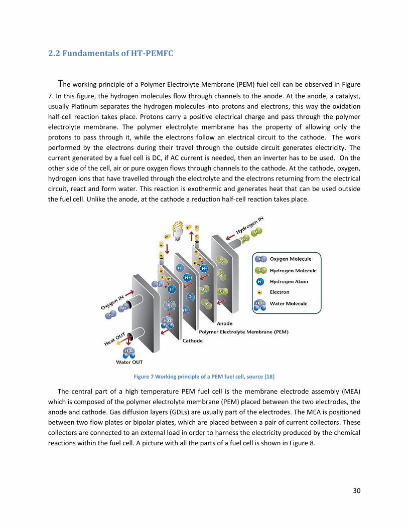
The working principle of a Polymer Electrolyte Membrane (PEM) fuel cell can be observed in Figure

7. In this figure, the hydrogen molecules flow through channels to the anode. At the anode, a catalyst,

usually Platinum separates the hydrogen molecules into protons and electrons, this way the oxidation

half-cell reaction takes place. Protons carry a positive electrical charge and pass through the polymer

electrolyte membrane. The polymer electrolyte membrane has the property of allowing only the

protons to pass through it, while the electrons follow an electrical circuit to the cathode. The work

performed by the electrons during their travel through the outside circuit generates electricity. The

current generated by a fuel cell is DC, if AC current is needed, then an inverter has to be used. On the

other side of the cell, air or pure oxygen flows through channels to the cathode. At the cathode, oxygen,

hydrogen ions that have travelled through the electrolyte and the electrons returning from the electrical

circuit, react and form water. This reaction is exothermic and generates heat that can be used outside

the fuel cell. Unlike the anode, at the cathode a reduction half-cell reaction takes place.

Figure 7 Working principle of a PEM fuel cell, source [18]

The central part of a high temperature PEM fuel cell is the membrane electrode assembly (MEA)

which is composed of the polymer electrolyte membrane (PEM) placed between the two electrodes, the

anode and cathode. Gas diffusion layers (GDLs) are usually part of the electrodes. The MEA is positioned

between two flow plates or bipolar plates, which are placed between a pair of current collectors. These

collectors are connected to an external load in order to harness the electricity produced by the chemical

reactions within the fuel cell. A picture with all the parts of a fuel cell is shown in Figure 8.

31

Figure 8 Parts of a HT-PEMFC single cell, source [30]

Different membranes have been identified for HT-PEM fuel cells, and a classification of these

membranes was realized by Li et al. [25]:

- Modified perfluorosulphonic acid (PFSA) membranes

- Partially fluorinated and aromatic hydrocarbon polymers membranes

- Inorganic-organic composites

- Acid-base polymer membranes

Acid-base polymer membranes consist of a basic polymer doped with an inorganic acid or blended

with a polymeric acid. The basic polymer from this membrane acts as a proton acceptor. The protons

have to be donated by strong or medium strong acids. Such acids could be phosphoric or phosphonic

acids due to their amphoteric character. The use of amphoteric acids, which presents both the acidic

(proton donor) and basic (proton acceptor) groups, seems to result in a high conductivity of the

membrane [25]. Other reasons of using these acids at elevated temperatures are their thermal stability

and low vapor pressure [25].

Better features of membranes used in high temperature PEM fuel cells such as high conductivity,

good mechanical properties, and excellent thermal and chemical stability, durability were achieved with

the development of acid-doped polybenzimidazole (PBI) membranes [25]. In addition, low cost can also

be included among the advantages of these membranes. PBI is a family of aromatic heterocyclic

polymers which contain benzimidazole units [25]; the chemical structure of a PBI repeated unit is given

in Figure 9.

Some of the main functions of a membrane in fuel cells are: must exhibit relatively high proton

conductivity, acts as an interface for the chemical reactions that take place at the electrodes, serves as a

support for the catalyst and the two electrodes and must be chemically and mechanically stable in the

32

fuel cell environment [25]. Moreover, membranes in fuel cells must block the migration of gaseous

reactants from one electrode to the other.

Figure 9 Chemical structure of PBI repeat unit, source [22]

The electrodes consist of the gas diffusion layer (GDL) which is made of porous carbon layers and the

catalyst layer (CL) where the Pt nano-particles are dispersed on a carbon support. The electrochemical

reactions take place on the catalyst surface. This is the reason why the loading of Platinum on electrodes

has been reduced along time. Catalyst surface area is very important for the processes occurring during

the operation of a fuel cell, and not the weight [31]. The gas diffusion layers require some properties

such as: to be sufficiently porous in order to allow the flow of reactant gases, electrically and thermally

conductive and sufficiently rigid [31].

Bipolar plates or flow plates are usually made from graphite and have to fulfill the following

requirements: high electrical conductivity, low gas permeability, high corrosion resistance, sufficient

strength, low thermal resistance, and so on [22]. In order to prevent leakage of reactant gases from the

fuel cells, gaskets are used, which are made of silicon rubber.

2.3 Degradation of HT-PEMFC

In order to replace the existing technologies, fuel cells have to meet some requirements, such as the

ones established by the U.S. Department of Energy (DOE) [13, 32]: a lifetime of 5000 hours as in the case

of transportation application, 40,000 hours of steady state operation for stationary systems and to

perform over the full range of operating temperatures (-40 oC – 40 oC) with a loss in performance less

than 10 %. PBI-based HT-PEMFCs operation has been demonstrated for more than 17,000 hours under

steady state conditions such as: 150 oC, 0.2 A/cm2, a hydrogen stoichiometry of 1.2 and of 2 for air [32].

Compared to Nafion-based PEM fuel cells, the PBI-based HT-PEM fuel cells presents some

advantages, among which: higher resistance to fuel impurities, easier water management due to the

absence of liquid water, lower performance and durability and it is more attractive for the use in

stationary systems where the fuel is produced on-site via steam reforming [32].

33

The limited lifetime is the main barrier to the commercialization of this technology. That is why

research has been ongoing to study the behavior of these fuel cells under different operating conditions.

The studies include durability and accelerated stress tests.

Durability is “the ability of a fuel cell to resist to permanent changes in performance over the time”

[22, 33], while the accelerated stress tests include three types of tests: screening tests, mechanistic tests

and lifetime tests [34]. Screening tests are used to determine the relative durability of one component

of a fuel cell, such as membrane, catalysts and GDLs, whereas mechanistic tests determine the failure

kinetics and pathways [34].

The durability and lifetime of a high temperature PEM fuel cell can be improved if the degradation

modes and the respective mitigation strategies are understood. There are three types of degradation

modes in a HT-PEMFC: thermal, chemical and mechanical mechanisms [47].

For example in the case of membranes, mechanical damage includes cracks, punctures, or pinhole

formation which can be generated by reactants crossover [35]. High temperature can also increase the

degradation of polymer membranes, especially the degradation of very thin membranes. For example

the research [32] showed that the voltage degradation rate increases from a few µV/h to some tens of

µV/h when the temperature is varied from 150 oC to around 200 oC. Moreover, an incomplete oxygen

reduction reaction (ORR) can generate hydrogen peroxide that can attack chemically the membrane

[35]. Another factor that can have an effect on membrane degradation can be the operation conditions

such as the startup/shutdown cycles, load variations [32].

The catalyst, Platinum in the case of HT-PEMFCs, is another important component whose

degradation has been studied. It seems that the performance of fuel cells is affected by the

agglomeration of the Pt particles by a process called Ostwald ripening process [36]. Ref. [32] also

believes that the presence of phosphoric acid within the MEA is another factor that may affect the

durability of HT-PEMFCs, by creating harsher working conditions. The same source [32] showed that

high temperatures also enhance the degradation of the carbon support.

Furthermore, the literature research conducted by [32] concluded that there are three mechanisms

by which degradation takes place: corrosion of the catalyst carbon support, degradation of the polymer

electrolyte membrane and acid leaching. However, degradation tests are also affected by the absence of

test protocols and the limited number of investigated steady state conditions [32].

34

2.4 HT-PEMFC characterization techniques

Polarization curve

Polarization curve or I-V curve represents the fuel cell losses as function of current density. The

different losses that may occur in a fuel cell can be classified as: activation losses resulted from the

energy needed to activate the reactions in the fuel cell; the Ohmic losses resulted due to resistance in

electrodes, plates, proton transport in the membrane and the concentration losses, which cause the

voltage to drop due to mass transport limitations [37]. A typical polarization curve for a PEM fuel cell

with the various loss-regions can be seen in Figure 10.

Figure 10 Polarization curve of a PEM fuel cell with the various loss-regions, source [37]

Electrochemical impedance spectroscopy (EIS)

I-V curves alone are not sufficient to understand the degradation mechanisms that take place in a

fuel cell. Some other characterization techniques are required to study the losses within a fuel cell and

the impact of the different electrochemical, chemical and thermodynamic processes on the

performance of a fuel cell [38]. An efficient way to do it is by using electrochemical impedance

spectroscopy (EIS), which is a measurement technique of the ability of an electrical circuit to resist the

flow of electrical current. This is realized by inducing small signal perturbances in a dynamic system to

measure the electrical response over a wide range of frequencies. This response is then analyzed in

order to obtain information about the system’s physicochemical properties.

35

Like resistance, impedance can be described by a relation between voltage and current:

Eq. (14)

, where is the complex impedance response of a system, represents the voltage, is

the current signal,

is the signal frequency and is the voltage phase shift. Since

impedance is represented as a complex number, the expression is composed of a real part ( )

and an imaginary part ( ). When the imaginary part is represented as function of real part,

Nyquist plot is obtained. Such a plot can be observed in Figure 11.

Figure 11 Nyquist plot, source [22]

When the electrochemical impedance of a fuel cell is measured, normally a small perturbation (AC

signal between 1 to 10 mV) is applied to the cell, which must be at steady state throughout time [39].

But in reality, it is very hard to achieve steady state in a cell due to all the changes that take place inside

the cell such as: adsorption of impurities coming from the anode feed gas, growth of an oxide layer,

coating degradation or even temperature changes [39].

More accurate information about the electrical performance of a fuel cell can be obtained if the

measured data of electrochemical impedance is fitted to an Equivalent Circuit (EC) model, which uses

basic electrical circuit components such as resistors, inductors or capacitors. The impedances of circuit

elements used in the equivalent circuit models can be seen in Table 3.

36

Table 3 Circuits elements used in the EC models, adapted from [39]

Equivalent element Current vs. Voltage Impedance

Resistor (R) V = IR Z = R

Capacitor (C) V = L

Z = 1/

Inductor (L) I = C

Z =

The current through these circuit elements behaves differently, for example due to the fact that the

impedance of a resistor has no imaginary component and is independent of frequency, the current

through a resistor is in phase with the voltage [39]. In the case of an inductor, whose impedance

increases as frequency increases, the current is phase-shifted -90o with respect to the voltage [39]. The

impedance of a capacitor is opposite to that of an inductor.

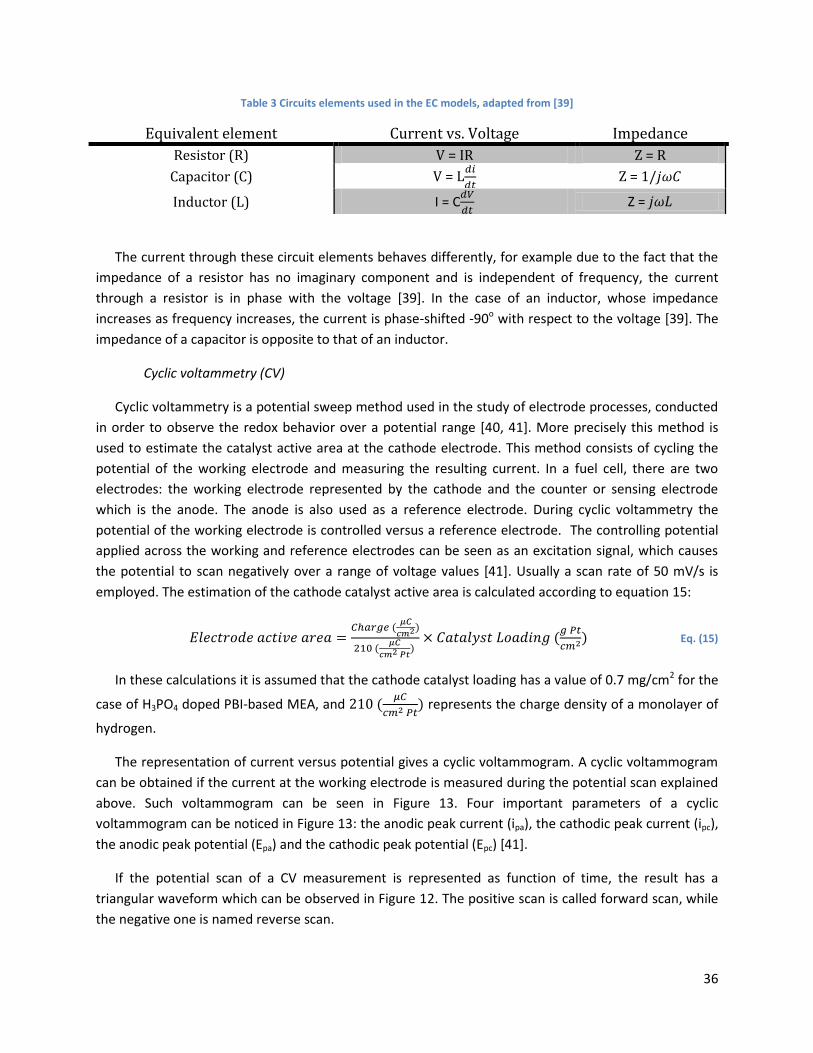
Cyclic voltammetry (CV)

Cyclic voltammetry is a potential sweep method used in the study of electrode processes, conducted

in order to observe the redox behavior over a potential range [40, 41]. More precisely this method is

used to estimate the catalyst active area at the cathode electrode. This method consists of cycling the

potential of the working electrode and measuring the resulting current. In a fuel cell, there are two

electrodes: the working electrode represented by the cathode and the counter or sensing electrode

which is the anode. The anode is also used as a reference electrode. During cyclic voltammetry the

potential of the working electrode is controlled versus a reference electrode. The controlling potential

applied across the working and reference electrodes can be seen as an excitation signal, which causes

the potential to scan negatively over a range of voltage values [41]. Usually a scan rate of 50 mV/s is

employed. The estimation of the cathode catalyst active area is calculated according to equation 15:

Eq. (15)

In these calculations it is assumed that the cathode catalyst loading has a value of 0.7 mg/cm2 for the

case of H3PO4 doped PBI-based MEA, and

represents the charge density of a monolayer of

hydrogen.

The representation of current versus potential gives a cyclic voltammogram. A cyclic voltammogram

can be obtained if the current at the working electrode is measured during the potential scan explained

above. Such voltammogram can be seen in Figure 13. Four important parameters of a cyclic

voltammogram can be noticed in Figure 13: the anodic peak current (ipa), the cathodic peak current (ipc),

the anodic peak potential (Epa) and the cathodic peak potential (Epc) [41].

If the potential scan of a CV measurement is represented as function of time, the result has a

triangular waveform which can be observed in Figure 12. The positive scan is called forward scan, while

the negative one is named reverse scan.

37

Cycle 1

Figure 12 Current vs. time

Figure 13 Cyclic voltammogram, source [41]

38

39

3 Methodology

This chapter describes the test set-up, the measurement instruments and experimental procedure

used in the current work, together with some characteristics of the MEAs and fuel cell components.

3.1 Description of the test set-up

The MEAs used in this research are Celtec® P2100 from BASF and Dapozol® G77 from Danish Power

System. Some details of the MEAs are given in Table 3 and Table 5, while Table 4 presents the

specifications of the other fuel cell components. Some information was not revealed by the respective

companies, that is why the secret information appears as “Proprietary Information”. In addition, a

picture of the flow channels is illustrated in Figure 14.

According to [32], the BASF Celtec® P2100 MEA is produced by direct casting via a sol-gel process.

Usually the Pt loading at the anode electrode is of 1.0 mg/cm2, while at the cathode electrode the

loading is of 0.7 mg/cm2. In the study performed by [32], the active area was of 20 cm2, while in the

present study the active area is of 49 cm2.

The MEA was mounted inside an in-house made fuel cell structure composed of two bipolar plates

(one for the anode side and the other for the cathode side), two current collector plates and two end

plates. Between the MEA and bipolar plates a gasket is used for each side to prevent leakages. A double

serpentine flow channel was used for the anode bipolar plate and a triple serpentine distributor was

mounted at the cathode to limit the pressure drops of air. In the case of anode, the pressure drops are

more limited, that is why a double serpentine distributor is sufficient. The reactant gases are fed in

counter flow configuration to the anode and cathode side respectively.

Table 4 Details of tested single cell

MEA manufacturer BASF Danish Power System

Fuel cell technology HT-PEMFC HT-PEMFC Cell model Celtec® P2100 Dapozol® G77

Product tested Membrane-Electrode unit Membrane-Electrode unit Product number 3M111191801 DPSRD-13-01 Identity number 144440-000565-3 RD-13-01

40

Table 5 Details of the fuel cell components


Fuel cell: material/coating of the bipolar plates

Graphite Graphite

Fuel cell: flow field design

Anode plate: double serpentine flow channel

Cathode plate: triple serpentine flow channel

Anode plate: double serpentine flow channel

Cathode plate: triple serpentine flow channel

Fuel cell: active area (cm2) 49 49 Gasket type PTFE PTFE

Gasket thickness (µm) 150 250 Cell technology (collectors) - -

Cell tightening (Nm) 280 300 Gas flow direction Counter flow Counter flow

Table 6 Specifics of the MEA components


MEA assembling Proprietary information Proprietary information Electrodes Proprietary information Proprietary information

Gas diffusion layers (thickness, µm) Proprietary information 250 Catalyst layer cathode (loading,

composition) Proprietary information Proprietary information

Catalyst layer anode (loading, composition)

Proprietary information Proprietary information

Anode Pt loading [mg/cm2] 0.7 – 1 1.6 Cathode Pt loading [mg/cm2] 0.7 – 1 1.6

Membrane (type) H3PO4 doped PBI H3PO4 doped PBI H3PO4 doping level (H3PO4 molecules/PBI

unit) Proprietary information 9

Figure 14 Flow fields design

41

The fuel cell assembly was connected to the test bench – GreenLight Innovation G60B – which

consists of:

- PC including operation and data acquisition software (HyWARE II)– Labview based control

system – plus an automation system called HyAL, which allows for EIS or CV measurements

without interrupting the process control or without user interventions;

- Electronic load to draw current from the fuel cell;

- Mass flow controllers for the reactant gases;

- Electric heaters – 220V AC;

- Methanol injection system: methanol tank, metering pump and evaporator.

All the above components of the test bench can be observed in the schematic of the experimental

setup, illustrated in Figure 15. Additionally, a picture of the fuel cell used in the current work is shown in

Figure 16.

Figure 15 Schematic of the test set-up

The Labview based control system allows recording the different parameters of the performed

experiments every second, such as the voltage, current density, reactant gases temperatures,

impedance and cyclic voltammetry spectra, etc. Voltage data were used to analyze the voltage profile of

degradation experiments performed in the present work, while the impedance and voltammetry data

were collected using the Gamry Instruments Reference 3000 Potentiostat in a system with the

42

Reference 30k Booster. The use of both devices from Gamry Instruments was necessary in order to

extend the measureable current to 30 A. The Reference 3000 unit can scan at frequencies up to 1 MHz

with a maximum current output of 3 A, but when the system is boosted with a Reference 30k, the

measureable current increases to 30 A [42, 43].

Figure 16 Fuel cell picture

3.2 Experimental procedure

The calculation of inputs for the experiments performed in the current work are based on the

assumption that reformate gas obtained by steam reforming a mixture of methanol and water with a

steam to carbon (S/C) ratio of 1.5 is used as fuel for the high temperature PEM fuel cell. The reaction

that takes place during the steam reforming of methanol is given below:

Eq. (16)

As it can be observed from the above chemical formula, the products of methanol steam reforming

are: hydrogen ( ), carbon dioxide ( ), water vapor and unconverted methanol vapor,

. Small amounts of carbon monoxide (CO) result from secondary reactions that occur

during the reforming process. There are other two reactions that usually occur, namely the methanol

decomposition (eq. (17)) and the reverse water gas shift reaction (eq. (18)).

43

Eq. (17)

Eq. (18)

All these products represent the components of the anode feed gas for the high temperature PEM

fuel cell. The choice of a reformate gas as anode feed gas for the operation of a high temperature PEM

fuel cell is based on the assumption that hydrogen obtained from the reforming of hydrocarbons is a

better solution compared to hydrogen storage in terms of cost and infrastructure [18].

Moreover, methanol steam reforming is a process taking place at temperatures of about 250 – 300 oC, which makes it more advantageous due to the faster startup and lower costs compared to methane

steam reforming, which takes place at temperatures of around 750 – 900 oC [29]. In this case, all the

gases besides hydrogen in the anode feed gas are seen as impurities.

To isolate the effects of methanol slip, carbon dioxide (CO2) and carbon monoxide (CO) are not

considered in the present experimental matrix. Before describing the calculation steps of inputs used in

the current study, the startup procedure of the fuel cell and the activation test of the MEA should be

outlined.

The startup procedure consists in heating the single cell until the desired operating condition. During

this warm-up of the unit cell until the temperature of 100 oC, no fuel or oxidant is supplied. When the

temperature of end plates reaches 100 oC, the stoichiometry and temperature inlets of both gas streams

are set. Further on, when the flow rates are established, the test equipment is set for the load mode

control, where the load of the stack is increased slowly until the operating current. When the load is

reached, the voltage is left to stabilize for a period of time, at least 30 minutes. The stability criterion

described in the protocol from [45] is followed for this scope.

The activation or break-in test consists in running the single cell on pure hydrogen at a temperature

of 160 oC, a current of 10 A and a stoichiometry of reactant gases of 1.2 for hydrogen and 4 for air,

respectively. The break-in test varies from one MEA to another. In the case of BASF MEA, the break-in

test was performed for 100 hours, while for the Danish Power System MEA the break-in test held 25

hours.

In this study two types of experiments were performed: performance tests with the BASF Celtec®

P2100 MEA and degradation tests with the Danish Power System Dapozol® G77 MEA. Compared to

performance tests, whose main objective is to study the effect of temperature and methanol slip in

short time, the degradation tests aim to study the effect of methanol slip at a constant temperature for

longer periods of time (100 hours for each condition and a total duration of 500 hours – 600 hours).

The purpose of performance tests is to characterize, as the name implies, the performance of a HT-

PEM fuel cell under different operating temperatures and various methanol concentrations. The

different vapor mixture compositions are calculated according to the conversion of reactants. The

conversion of reactants (methanol and water) into products is considered to be 100 %, 98 %, 96 %, 94 %,

92 % and 90 %. Two additional experiments were performed with pure hydrogen at room temperature

and preheated hydrogen at 140 – 160 oC, as reference conditions. The inputs of the performance tests

44

conducted at 140 oC are shown in Table 7. These tests were repeated for each operating temperature up

to 180 oC, at a temperature increase step of 10 oC, at varying vapor compositions.

Table 7 Operating conditions and inputs of the performance tests conducted at 140 oC

Exp. ID Temperature (oC)

Yield (%) MeOH conc. (%)

H2O conc. (%)

1

140

Pure H2 (room temperature)

0 0

2 Preheat H2

(140 oC) 0 0

3 100 0 14.29 4 98 0.57 14.94 5 96 1.16 15.16 6 94 1.74 16.28 7 92 2.34 19.96 8 90 2.94 17.65

For the current performance tests, the MEA has a total active area of 49 cm2 and stoichiometry of 1.2

for hydrogen and of 4 for air is used. These values are chosen based on the compromises between the

efficiency of the fuel cell and the mass transport limitations [29]. All the performance tests are

conducted at a constant fuel cell current of 15 A. Based on these conditions, the volume flow rate of

hydrogen is calculated with equation 19, while the volume flow rate of air is obtained using equation 20:

(

) Eq. (19)

(

) Eq. (20)

The humidification of the reactant gases is performed by adjusting the dew point and gas

temperatures of the reactants. The dew point temperature of gaseous reactants is calculated with the

following equations:

[

(

)] Eq. (21)

Eq. (22)

Eq. (23)

[

] Eq. (24)

In the case of degradation tests, four types of experiments are performed; each experiment has

duration of approximately 100 hours. The experimental matrix for the four types of experiments is

shown in Table 8.

45

Table 8 Operating condition and inputs of the degradation tests

Exp. ID

Type of experiment

Description

1 H2 continuous 160 oC;

; 15 A; Preheat H2;

100 hours

2 H2 start/stop

Start period:

12 hours; 160 oC;

; 15 A

Preheat H2

Stop period: 12 hours; Room temperature

No gas flow; 0 A

100 hours total

3 MeOH

continuous

160 oC;

; 15 A; Preheat H2; MeOH concentration = 3%

100 hours

4 MeOH

start/stop

Start period:

12 hours; 160 oC;

; 15 A;

Preheat H2 MeOH concentration = 3%

Stop period: 12 hours; Room temperature

No gas flow; 0 A

100 hours total

For each experiment, polarization curves and impedance spectra are measured. In the case of

performance tests, voltammetry data are also collected. Besides these characterization techniques,

different parameters such as voltage, current density and reactant gases temperatures were data logged

during all the experiments in order to analyze the voltage decay rate, which is very important when

degradation tests are studied.

3.2.1 Polarization curve – measurement technique

The main objective of the polarization curve is to determine the change in the single cell voltage

generated by varying different conditions such as the operating temperatures from 140 oC to 180 oC,

with an increase step in temperature of 10 oC, or the methanol concentrations or the dew points of

anode feed gas inlet. A script is created using the automation system HyAL to help to the measurement

of I-V curves. This script can be found in Appendix C.

Voltage data is recorded every second during degradation experiments in order to analyze voltage

behavior in time. Due to the huge amount of recorded data, a Matlab script, which can be found in

Appendix A, is used to calculate the average of every 10 minutes of data logging. The average of 10

minutes represents a single voltage point in the graphical representation of voltage as function of time.

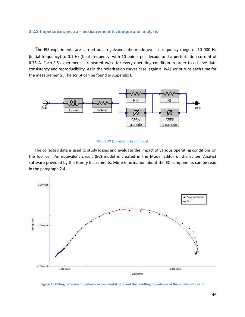
46

3.2.2 Impedance spectra – measurement technique and analysis

The EIS experiments are carried out in galvanostatic mode over a frequency range of 10 000 Hz

(initial frequency) to 0.1 Hz (final frequency) with 10 points per decade and a perturbation current of

0.75 A. Each EIS experiment is repeated twice for every operating condition in order to achieve data

consistency and reproducibility. As in the polarization curves case, again a HyAL script runs each time for

the measurements. The script can be found in Appendix B.

Figure 17 Equivalent circuit model

The collected data is used to study losses and evaluate the impact of various operating conditions on

the fuel cell. An equivalent circuit (EC) model is created in the Model Editor of the Echem Analyst

software provided by the Gamry Instruments. More information about the EC components can be read

in the paragraph 2.4.

Figure 18 Fitting between impedance experimental data and the resulting impedance of the equivalent circuit

47

The EC model used in the analysis of impedance spectra is shown in Figure 17 and is composed of an

inductor (Lstray) in series with a resistance (Rohmic) and two circuits, each comprising a resistance and a

constant phase element (CPE), parallel to each other. The values of different components of the

equivalent circuit are obtained by fitting the resulting impedance of the circuit with the experimental

impedance data. In this study, a complex non-linear least square (CNLS) method is used to fit the

equivalent circuit impedance with the experimental one. More about non-linear least square fitting

techniques of impedance data can be read in [49]. An example of the fit between the experimental

impedance data and the resulting impedance of the equivalent circuit model showing its quality is given

in Figure 18.

The Nyquist plot of the collected impedance data revealed two loops: one high frequency loop and

another one low frequency. As one can see in Figure 19, the ohmic resistance is represented by the

intercept of the high-frequency impedance loop with the real axis. This resistance corresponds to the

ohmic losses of the unit cell. These losses occur mainly due to electrolyte resistances, catalyst layer,

bipolar plates or contact resistances between them [29, 37]. Of all these resistances, the membrane

resistance is the main responsible of the overall ohmic resistance [37]. According to Ref [37], this

resistance can be minimized by reducing the thickness of the membrane or by using a membrane with

higher conductivity. These however, could make the membrane less resistant to mechanical

degradation.

The high frequency and low frequency resistances are connected in parallel with a constant phase

element (CPE). This connection in parallel forms two arcs which reflect the charge transfer resistances

due to the anode or cathode activation losses. Better fits are achieved if CPEs are used instead of double

layer capacitances [29, 38]. The impedance of a CPE is given in the below equation:

Eq. (25)

, where represents the time constant and is the phase angle. This element presents the

advantage that can behave as a resistor if and , as a capacitor if and

or as a inductor if and [38].

The inductor is used to reflect the losses which may occur due to wiring and other instrumental non-

idealities [28].

3.2.3 Cyclic voltammetry – measurement technique and analysis

Cyclic voltammetry measurement technique is used to estimate the catalyst active area of the

cathode electrode. At the cathode the kinetic losses are very important due to the slow oxygen

reduction reaction (ORR) [32].

48

Ohm

ic lo

sses

Prot

on t

rans

fer

loss

Charge transfer loss

Mass transfer loss

Figure 19 Specifications of the equivalent circuit model

During these measurements, the fuel cell operation is interrupted. The anode side is fed with

hydrogen, while nitrogen is used for the cathode side. The anode is taken as the reference and counter

electrode, while the cathode is the working electrode.

The potential of the working electrode is continuously scanned back and forth between voltages of

0.05 V and 1 V. Three cycles are measured, with an initial delay of 5 seconds (in order to ignore the

initial inaccurate data), a sample interval of 0.1 seconds and a scan rate of 0.05 V/sec. The three cycles

are necessary for activating and purifying the electroactive Pt surface from possible impurities. The

actual measurement used in the graphical representations is taken from the second cycle.

From this voltammetric cycle, the hydrogen desorption charge is obtained by determining a baseline

on the positive branch of the voltammogram and integrating between potentials of 0.1 and 0.4 V above

this baseline. The software Echem Analyst provided by Gamry Instruments is a good tool to realize these

steps. The method used is followed according to the steps described in Ref. [41]. The cathode catalyst

active area is estimated with equation 15.

49

4 Results & Interpretation

In this section the effects of temperature and methanol slip on the performance and degradation of

the H3PO4 doped PBI-based HT-PEM fuel cells are described based on the analysis of data acquired during

experiments. This section is divided in two parts: performance tests and degradation tests.

4.1 Performance tests

As already mentioned in the experimental procedure, the main objective of performance tests is to

study the effect of temperature and methanol slip during short periods of time. These types of tests

were performed on a BASF Celtec® P2100 MEA. For this scope, polarization curves together with the

impedance and cyclic voltammetry collected data during the experiments are analyzed. The EIS spectra,

cyclic voltammograms and polarization curves are measured according to the procedures described in

paragraphs 3.2.1 – 3.2.3.

4.1.1 Effect of operating temperature

According to polarization curves measured during the performance tests, the performance of the

cell increases as temperature increases. This effect is observed in both tests conducted with pure

hydrogen as anode feed gas. In one test hydrogen is used at room temperature, while the other test

uses hydrogen preheated at a temperature of 140 oC. There are no significant changes in the voltage-

current density profile if preheated hydrogen is used instead of hydrogen at room temperature.

For example, at a voltage of 0.34 V the current density at 140 oC is 1132.98 mA/cm2 for the case with

hydrogen at room temperature test, and 1132.78 mA/ cm2 for the preheated hydrogen performance

test. As temperature increases, current density is also increasing, reaching 1310 mA/cm2 for the

performance tests conducted at 180 oC at the same value for voltage. The polarization curves for the

two experiments are illustrated in Figures 20 and 21.

The EIS measurements conducted on the two performance experiments realized with pure hydrogen

at room temperature and preheated at a temperature of 140 oC showed the same effect observed by

the analysis of the polarization curves. Preheating the anode feed gas until the operating temperature

has almost few or no effect on the single cell. The EIS spectra of the two experiments can be observed in

Figures 22 and 23, while the fitted resistances are shown in Figures 30, 32 and 34.

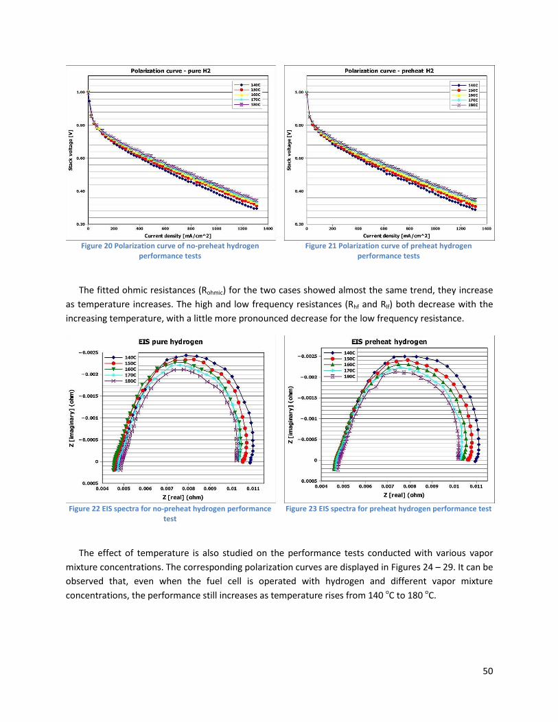
50

Figure 20 Polarization curve of no-preheat hydrogen

performance tests

Figure 21 Polarization curve of preheat hydrogen

performance tests

The fitted ohmic resistances (Rohmic) for the two cases showed almost the same trend, they increase

as temperature increases. The high and low frequency resistances (Rhf and Rlf) both decrease with the

increasing temperature, with a little more pronounced decrease for the low frequency resistance.

Figure 22 EIS spectra for no-preheat hydrogen performance

test

Figure 23 EIS spectra for preheat hydrogen performance test

The effect of temperature is also studied on the performance tests conducted with various vapor

mixture concentrations. The corresponding polarization curves are displayed in Figures 24 – 29. It can be

observed that, even when the fuel cell is operated with hydrogen and different vapor mixture

concentrations, the performance still increases as temperature rises from 140 oC to 180 oC.

51

Figure 24 Polarization curve of 100% conversion

performance tests

Figure 25 Polarization curve of 98% conversion performance

tests


tests


tests


tests


tests

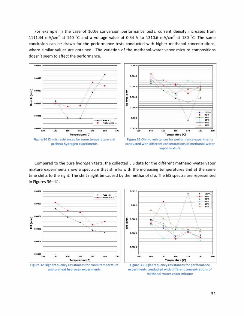
52

For example in the case of 100% conversion performance tests, current density increases from

1111.44 mA/cm2 at 140 oC and a voltage value of 0.34 V to 1310.6 mA/cm2 at 180 oC. The same

conclusion can be drawn for the performance tests conducted with higher methanol concentrations,

where similar values are obtained. The variation of the methanol-water vapor mixture compositions

doesn’t seem to affect the performance.

Figure 30 Ohmic resistances for room temperature and

preheat hydrogen experiments

Figure 31 Ohmic resistances for performance experiments

conducted with different concentrations of methanol-water vapor mixture

Compared to the pure hydrogen tests, the collected EIS data for the different methanol-water vapor

mixture experiments show a spectrum that shrinks with the increasing temperatures and at the same

time shifts to the right. The shift might be caused by the methanol slip. The EIS spectra are represented

in Figures 36– 41.

Figure 32 High frequency resistances for room temperature

and preheat hydrogen experiments

Figure 33 High-frequency resistances for performance

experiments conducted with different concentrations of methanol-water vapor mixture

53

Figure 34 Low frequency resistances for room temperature

and preheat hydrogen experiments

Figure 35 Low-frequency resistances for performance

experiments conducted with different concentrations of methanol-water vapor mixture

The increase in temperature causes the all fitted resistances to decrease. The fitted ohmic

resistances for the vapor mixture based experiments (Figure 31) show a behavior which is in contrast

with the one for the cases with pure hydrogen. Water vapor enhances the proton conduction of the

MEA and therefore decreasing the ohmic resistances. This conclusion is based on the comparison of the

ohmic resistance profiles between pure hydrogen tests and performance tests with 100 % reactants

conversion.

The low and high frequency resistances follow the same trend as the ones for pure hydrogen

performance tests (Figure 33 and 35). The fitted resistances for each performance experiment realized

with different vapor compositions are attached in Appendix D.

Figure 36 EIS spectra for 100% conversion performance

test

Figure 37 EIS spectra for 98% conversion performance test

54





The catalyst active area is measured by cyclic voltammetry according to the procedure described in

paragraph 3.2.3. Based on the steps described by the mentioned procedure, the hydrogen desorption

charges obtained for the performance experiments realized with different vapor mixture concentrations

are given in Table 9. Using the equation 15 and the values obtained in Table 9, the cathode catalyst

active area is estimated in Table 10. In these calculations it is assumed that the cathode catalyst loading

has a value of 0.7 mg/cm2 and

represents the charge density of a monolayer of hydrogen.

The values obtained for the estimated cathode catalyst active area increase as temperature

increases. An exception takes place at the temperature of 160 oC, where in all cases the active area

decreases. The increase in the active area could explain for example the Platinum nano-particles

agglomeration process, also known as the Ostwald ripening process.

The loss of active area can be described by three different mechanisms [32]: carbon corrosion,

thinning of the catalyst layer and dissolution and sintering of the Platinum particles. The phosphoric acid

55

present in the PBI-based MEA can dissociate during the fuel cell operation and generate phosphate

anions (H2PO4-). These anions could be adsorbed onto the platinum particles in various amounts and this

way hinders the oxygen reduction [32]. During CV measurements, the adsorption of the anions is forced

and appears in the cyclic voltammograms as distortions in the shape or as peaks [32].

The same source [32] conducted a degradation test on a BASF Celtec P2100 MEA with pure hydrogen

and air at temperature of 160oC and 180oC. They found out that the increase in temperature accelerates

the degradation of the MEA.

Table 9 Hydrogen desorption charge (mC)

Conversion rate (%)

Temperature (oC)

140 150 160 170 180 100 432.5 447.7 326.7 534.2 548.1 98 395.1 409.6 286.0 456.5 466.8 96 330.1 418.5 266.8 426.0 458.0 94 315.9 373.2 258.8 448.3 452.3 92 400.2 387.2 215.6 382.1 420.3 90 439.5 430.7 115.9 396.9 418.8

Table 10 Estimated cathode catalyst active area (cm2)

Conversion rate (%)

Temperature (oC)

140 150 160 170 180 100 0.029 0.030 0.022 0.036 0.037 98 0.027 0.028 0.019 0.031 0.032 96 0.022 0.028 0.018 0.029 0.031 94 0.021 0.025 0.018 0.030 0.031 92 0.027 0.026 0.015 0.026 0.029 90 0.030 0.029 0.008 0.027 0.028

The cyclic voltammograms presented in Figures 42 – 46 show the little effect of temperature at 150 oC and 180 oC. At the temperatures of 140 oC and 170 oC, the current – voltage profiles decrease with the

increase of the methanol concentration in the anode feed. The same trend is observed in the case of

cyclic voltammograms measured at 160 oC for reactants conversion of 100 %, 98%, 96%, 94%.

The current – voltage profiles of the experiments conducted at 160 oC with a reactant conversion of

92 % and 90% (Figure 44) are very different compared to the other experiments. This profile might be

an effect of the methanol slip in the anode feed gas.

56

Figure 42 Cyclic voltammogram of performance tests at

140 oC


150 oC

Figure 44 Cyclic voltammogram of performance tests at 160 oC


170 oC


180 oC

57

4.1.2 Effect of methanol slip

The effect of methanol slip is studied at a constant temperature of 160 oC for the performance tests

when the concentrations of methanol-water vapor mixture are varied. The variation of the methanol

concentrations doesn’t seem to affect the performance of the fuel cell. This issue can be observed in

Figure 47, where the voltage vs. current density profile of the performance tests conducted with

different vapor mixture concentrations at a constant temperature of 160 oC is shown.

Figure 47 Polarization curve of performance tests conducted with different vapor mixture concentrations at a constant temperature of 160

oC

The poisoning effect of methanol-water vapor mixture at all frequency sweeps can be observed in

Figure 48. The fitted resistances for these performance tests are shown in Figure 49. At constant

temperature, the low-frequency resistance slightly decreases with the increase in vapor mixture

concentration. The same thing can be said about the ohmic resistances, where the variations in vapor

mixture concentration do not have a significant effect, while in the case of high-frequency resistances, a

slight increase is observed with the raise in the concentration of methanol-water vapor mixture.

Figures 50 – 55 present the effect of the methanol slip on the current – voltage profiles. At first sight,

the methanol slip seems of not having an effect on the curves. Approximately all the curves follow the

same trend. However, one can notice the effect of temperature on the curves. The increasing

temperature leads to the appearance of an extra peak on the curves, which becomes more pronounced

at higher temperatures (170 oC and 180 oC).

However, Ref. [32] suggested another explication of the appearance of peaks on the CV curves. Peak

appearance is related to the adsorption of the phosphate anions onto the platinum surface.

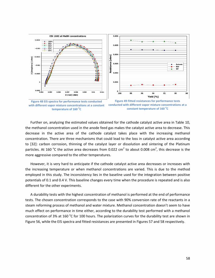
58

Figure 48 EIS spectra for performance tests conducted

with different vapor mixture concentrations at a constant temperature of 160

oC

Figure 49 Fitted resistances for performance tests

conducted with different vapor mixture concentrations at a constant temperature of 160

oC

Further on, analyzing the estimated values obtained for the cathode catalyst active area in Table 10,

the methanol concentration used in the anode feed gas makes the catalyst active area to decrease. This

decrease in the active area of the cathode catalyst takes place with the increasing methanol

concentration. There are three mechanisms that could lead to the loss in catalyst active area according

to [32]: carbon corrosion, thinning of the catalyst layer or dissolution and sintering of the Platinum

particles. At 160 oC the active area decreases from 0.022 cm2 to about 0.008 cm2, this decrease is the

more aggressive compared to the other temperatures.

However, it is very hard to anticipate if the cathode catalyst active area decreases or increases with

the increasing temperature or when methanol concentrations are varied. This is due to the method

employed in this study. The inconsistency lies in the baseline used for the integration between positive

potentials of 0.1 and 0.4 V. This baseline changes every time when the procedure is repeated and is also

different for the other experiments.

A durability tests with the highest concentration of methanol is performed at the end of performance

tests. The chosen concentration corresponds to the case with 90% conversion rate of the reactants in a

steam reforming process of methanol and water mixture. Methanol concentration doesn’t seem to have

much effect on performance in time either, according to the durability test performed with a methanol

concentration of 3% at 160 oC for 100 hours. The polarization curves for the durability test are shown in

Figure 56, while the EIS spectra and fitted resistances are presented in Figures 57 and 58 respectively.

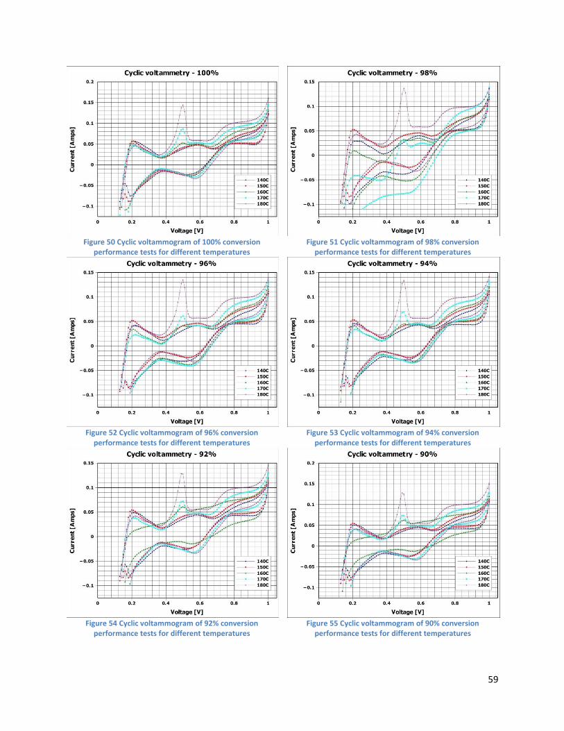
59

Figure 50 Cyclic voltammogram of 100% conversion

performance tests for different temperatures











60

Figure 56 Polarization curves for durability test with MeOH

Figure 57 EIS spectra for durability test with MeOH

Figure 58 Fitted resistances for durability test with MeOH

The ohmic and high-frequency resistances increase in time, while the low-frequency resistance

decreases in time. As mentioned earlier, ohmic resistance represents the contact resistances and

electrolyte resistance. The variation of methanol-water vapor concentrations has negligible effect on the

overall conductivity of the membrane (Figure 49). But in time, as one can notice in Figure 58, methanol-

water vapor concentration might affect the membrane conductivity, an increase in ohmic resistance

being observed after 40 hours of operation at 160 oC, after which it stabilizes.

To summarize, temperature and methanol-water vapor mixture affects the performance of a

phosphoric acid doped PBI-based MEA. As outlined earlier, the increase in temperature improves the

performance of the MEA during the experiments conducted with pure hydrogen, either preheated or

not, but can also degrade it more aggressively at the same time. The charge transfer losses in a

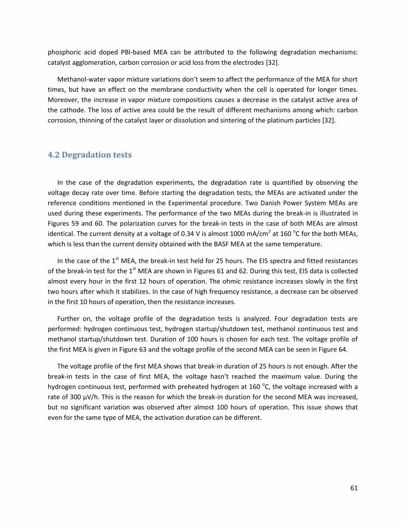
61

phosphoric acid doped PBI-based MEA can be attributed to the following degradation mechanisms:

catalyst agglomeration, carbon corrosion or acid loss from the electrodes [32].

Methanol-water vapor mixture variations don’t seem to affect the performance of the MEA for short

times, but have an effect on the membrane conductivity when the cell is operated for longer times.

Moreover, the increase in vapor mixture compositions causes a decrease in the catalyst active area of

the cathode. The loss of active area could be the result of different mechanisms among which: carbon

corrosion, thinning of the catalyst layer or dissolution and sintering of the platinum particles [32].

4.2 Degradation tests

In the case of the degradation experiments, the degradation rate is quantified by observing the

voltage decay rate over time. Before starting the degradation tests, the MEAs are activated under the

reference conditions mentioned in the Experimental procedure. Two Danish Power System MEAs are

used during these experiments. The performance of the two MEAs during the break-in is illustrated in

Figures 59 and 60. The polarization curves for the break-in tests in the case of both MEAs are almost

identical. The current density at a voltage of 0.34 V is almost 1000 mA/cm2 at 160 oC for the both MEAs,

which is less than the current density obtained with the BASF MEA at the same temperature.

In the case of the 1st MEA, the break-in test held for 25 hours. The EIS spectra and fitted resistances

of the break-in test for the 1st MEA are shown in Figures 61 and 62. During this test, EIS data is collected

almost every hour in the first 12 hours of operation. The ohmic resistance increases slowly in the first

two hours after which it stabilizes. In the case of high frequency resistance, a decrease can be observed

in the first 10 hours of operation, then the resistance increases.

Further on, the voltage profile of the degradation tests is analyzed. Four degradation tests are

performed: hydrogen continuous test, hydrogen startup/shutdown test, methanol continuous test and

methanol startup/shutdown test. Duration of 100 hours is chosen for each test. The voltage profile of

the first MEA is given in Figure 63 and the voltage profile of the second MEA can be seen in Figure 64.

The voltage profile of the first MEA shows that break-in duration of 25 hours is not enough. After the

break-in tests in the case of first MEA, the voltage hasn’t reached the maximum value. During the

hydrogen continuous test, performed with preheated hydrogen at 160 oC, the voltage increased with a

rate of 300 µV/h. This is the reason for which the break-in duration for the second MEA was increased,

but no significant variation was observed after almost 100 hours of operation. This issue shows that

even for the same type of MEA, the activation duration can be different.

62

Figure 59 Polarization curve for the break-in test of 1

st

Danish Power System MEA

Figure 60 Polarization curve for the break-in test of 2

nd


Figure 61 EIS spectra for break-in

Figure 62 Break-in fitted resistances

The total voltage drop for operation on preheat hydrogen in a startup/shutdown test taken over a

period of 100 hours is of about -46.3 mV. In the presence of methanol-water vapor mixture which

corresponds to approximately 3% methanol in the anode feed gas, the voltage decay rate for the

continuous test is of -120 µV/h (over a period of 100 hours), while the degradation rate for the

startup/shutdown test is of -7.9 mV/h.

63

Break-in

H2 continuous test

H2 start/stop test

MeOH continuous test

Figure 63 Voltage profile for the 1st MEA

Break-inPreheat H2

MeOH continuous

MeOH start-stop

Figure 64 Voltage profile for the 2nd MEA

64

4.2.1 H2 continuous test

In the case of degradation tests conducted with continuous hydrogen, for the first MEA the

performance of the cell increased over the 100 hours of operation (equivalent of 5 days) – Figure 65. On

the contrary, the performance of the cell when the second MEA is used remained the same over 75

hours of operation (Figure 66).

Figure 65 Polarization curve for the hydrogen continuous

test of the 1st


Figure 66 Polarization curve for the hydrogen continuous

test of the 2nd


As mentioned above, during the hydrogen continuous test on the first MEA, voltage increased with a

rate of 300 µV/h (Figure 67). The ohmic resistance slightly decreases over the 100 hours duration. The

low frequency resistances follow approximately the same trend, while the high frequency resistances

increase with time. The fitted resistances are presented in Figure 68.

Figure 67 Voltage profile of the hydrogen continuous test

Figure 68 Fitted resistances for H2 continuous test

65

4.2.2 H2 startup/shutdown test

In the case of hydrogen startup/shutdown test, a total voltage decay of -46.3 mV is registered over

the entire duration of operation (100 hours). The total voltage drop happens after the third

startup/shutdown cycle as it can be observed from Figure 69. The voltage across the first three cycles

has been constant. A constant voltage is also noticed in the last two startup/shutdown cycles.

Figure 69 Voltage profile of the hydrogen startup/shutdown

test

Figure 70 Polarization curve for the hydrogen startup/shutdown test of the 1

st Danish Power System MEA

After the third startup/shutdown cycle, the decay in performance is remarked on the polarization

curves in Figure 70. This enormous drop might be caused by an emergency stop (e-stop) during the

operation of the fuel cell. However, such a large drop in voltage can’t be attributed solely to the e-stop.

When an e-stop occurs, the mass flow controllers are shut down and the load current is set to zero. This

can lead to condensation during the cooling down of the single cell, because water is still in vapor form

at 160 oC. In the representations of the voltage vs. time, these e-stops are removed.

A drop of approximately 245 mA/cm2 in current density occurred during the hydrogen

startup/shutdown test from a value of 1000.65 mA/cm2 in the first day of test at a voltage of 0.375 V to

755.34 mA/cm2 after 100 hours of operation at the same conditions.

Compared to the hydrogen continuous test, the ohmic and low-frequency resistances are the

opposite way in the hydrogen startup/shutdown test – Figure 71. The high-frequency resistance

increases in both cases.

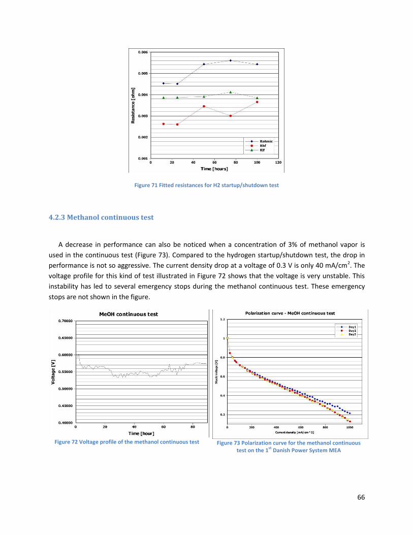
66

Figure 71 Fitted resistances for H2 startup/shutdown test

4.2.3 Methanol continuous test

A decrease in performance can also be noticed when a concentration of 3% of methanol vapor is

used in the continuous test (Figure 73). Compared to the hydrogen startup/shutdown test, the drop in

performance is not so aggressive. The current density drop at a voltage of 0.3 V is only 40 mA/cm2. The

voltage profile for this kind of test illustrated in Figure 72 shows that the voltage is very unstable. This

instability has led to several emergency stops during the methanol continuous test. These emergency

stops are not shown in the figure.

Figure 72 Voltage profile of the methanol continuous test

Figure 73 Polarization curve for the methanol continuous

test on the 1st


67

A recovery in the cell performance can be observed after a certain period in the methanol continuous

test. The total voltage drop is around 0.017 V over 100 hours of operation and the total recovery is of

0.0224 V over 40 hour of operation (Figure 72). The ohmic resistance shows a better stability in the

methanol continuous test, which leads to the conclusion that methanol-vapor concentration has

negligible effect on the overall conductivity of the membrane. The low-frequency resistance also

increases as in the hydrogen start/stop case, but the high-frequency resistance decreases.

Figure 74 Fitted resistances for MeOH continuous test

Based on the present results, one might conclude that the MEA presents better stability during the

methanol continuous test compared to the startup/shutdown test conducted with pure hydrogen.

However, this is not necessarily the case, since the sudden drop in voltage during the hydrogen

startup/shutdown test might not necessarily be due to the start/stop cycle itself.

4.2.4 Methanol startup/shutdown test

Surprisingly, over a period of 100 hours during the methanol startup/shutdown cycles, the cell

performance remained constant. At a voltage of 0.36 V and a temperature of 160 oC, the current density

is about 700 mA/cm2 and remained like that until the end of the experiment.

However, the methanol concentration used during the start-stop experiment might have a small

effect over the voltage if the age of the fuel cell is considered. This concentration was applied after the

fuel cell has been operated for the hydrogen continuous and methanol continuous tests. These tests

might have affected the cell somehow. Simon Araya et al. [46] conducted experiments in continuous

mode with the same concentration for the methanol-water vapor mixture, and they concluded that

charge transfer losses are the major contributor to the losses when a single cell is operated with 3%

vapor.

68

Figure 75 Voltage profile of the methanol startup/shutdown

test

Figure 76 Polarization curve for the MeOH start/stop test of

the 2nd


A comparison of fitted resistances between the methanol continuous test and methanol start/stop

test would have been interesting, but unfortunately due to some technical problems during the

methanol start/stop test, the recording of EIS data was not possible.

69

5 Conclusion & Future work

5.1 Final remarks

In this work, the performance and degradation of a phosphoric acid doped PBI-based HT-PEM fuel

cell is characterized by means of experimental testing. The effect of impurities from methanol steam

reforming process, more precisely the methanol-water vapor mixture and the effect of

startup/shutdown cycles were investigated by means of polarization curves, EIS and CV measurements.

Two types of experiments were performed: performance tests aimed to characterize the fuel cell in

the presence of different methanol-water vapor mixture concentrations and different temperatures and

degradation tests, whose scope was to study the startup/shutdown cycle effect on such fuel cell.

The fuel cell used in the performance experiments is a unit assembly of a 49 cm2 active area with a

BASF Celtec® P2100 MEA. For the degradation tests, a Danish Power System Dapozol® G77 MEA was

used instead of the BASF MEA in the same unit assembly.

The analysis of polarization curves, EIS spectra and cyclic voltammograms in the case of performance

tests recorded at different temperatures and different methanol-water vapor compositions shows that

the performance of the MEA is affected by temperature and the vapor impurities.

The increase in temperature improves the performance of the MEA during the experiments

conducted with pure hydrogen, but at the same time degrades the MEA even more aggressively as a

result of increasing cathode catalyst active area. This result is in accordance with the literature. The

charge transfer losses corresponding to the low frequency resistances decrease. These losses can be

attributed to the following degradation mechanisms: catalyst agglomeration, carbon corrosion or acid

loss.

Methanol-water vapor mixture variations don’t seem to affect the performance of the MEA for short

times, but certainly have an effect on the membrane conductivity when the cell is operated for longer

times. Moreover, the increase in vapor mixture compositions causes a decrease in the catalyst active

area of the cathode. According to literature, the loss of active area could be the result of different

mechanisms among which: carbon corrosion, thinning of the catalyst layer or dissolution and sintering

of the platinum particles.

Four types of degradation tests were conducted in the current study: hydrogen continuous test,

hydrogen startup/shutdown test, methanol continuous and startup/shutdown tests. During degradation

tests, the total voltage decay for operation on preheat hydrogen in the startup/shutdown test was of -

70

46.3 mV over a period of 100 hours. The total voltage drop during this test happened suddenly after the

third startup/shutdown cycle. It is very hard to conclude the reason of this drop, since this issue can’t be

attributed solely to an emergency stop. In the case of continuous hydrogen test, the voltage increased

with a rate of 300 µV/h.

Compared to the startup/shutdown cycles performed with pure hydrogen, the methanol

concentration (3%) had an effect on the voltage, by making it very unstable during the experiment. The

voltage instability caused the fuel cell system to go in emergency stops. A total voltage drop of around -

0.017 V was registered during the methanol continuous test and a recovery in the cell performance was

observed after a certain period.

The degradation rate during the methanol startup/shutdown test was the highest, -7.9 mV/h, but

compared to the hydrogen startup/shutdown and methanol continuous cases, the performance

remained constant.

5.2 Future work

For a better understanding of degradation mechanisms of phosphoric acid doped PBI-based HT-PEM

fuel cells, further work is needed for mitigating them and fasten the fuel cells commercialization

process.

A post-mortem analysis of the MEAs used in the present study could reveal the changes in the

platinum catalyst, and this way a better characterization of the degradation mechanisms can be

achieved. A further degradation test performed with pure hydrogen on another Danish Power System

MEA could help in understanding why such a voltage drop occurred during the startup/shutdown test.

And finally, a research could be conducted in order to study if methanol-water vapor mixtures have

an effect in phosphoric acid leaching.

71

6 References

[1] The World Bank, 2012, “What a waste – a global review of solid waste management”;

[2] IEO2011 (International Energy Outlook 2011), Release date: 19 September, 2011;

[3] Glen P. Peters, Robbie M. Andrew, Tom Boden, Josep G. Canadell, Philippe Ciais, Corinne Le Quéré,

Gregg Marland, Michael R. Raupach, Charlie Wilson, “ The challenge to keep global warming below 2

°C”, Nature Climate Change, 2012; DOI: 10.1038/nclimate1783;

[4] IEA 2012, “Global carbon-dioxide emissions increase by 1.0 Gt in 2011 to record high”, 24 May 2012,

http://www.iea.org/newsroomandevents/news/2012/may/name,27216,en.html, accessed 27/04/2013;

[5] IEA 2012, “Key world energy statistics”;

[6] BP Statistical Review of World Energy, June 2012;

[7] IEA, “Oil Market Report”, 13 February 2013;

[8] Renewables 2012, Global Status Report, REN21, Renewable Energy Policy Network for the 21st

Century;

[9] Intergovernmental Panel on Climate Change (IPCC), http://www.ipcc-data.org/, accessed

30/04/2013;

[10] LBST, http://www.lbst.de/publications/presentations2007/LBST_HYSYDays_6-

8JUN2007_Torino.pdf, accessed 25/04/2013;

[11] United Nations Environment Programme (UNEP),

http://www.unep.org/climatechange/mitigation/Bioenergy/Issues/TraditionaluseofBiomass/tabid/2947

3/Default.aspx, accessed 26/05/2013;

[12]

http://www.cheng.cam.ac.uk/research/groups/electrochem/JAVA/electrochemistry/ELEC/l10html/main

.html, accessed 01/05/2013;

[13] Department of Energy, Office of Science, Basic Research Needs for the Hydrogen Economy,

http://www.sc.doe.gov/bes/hydrogen.pdf, accessed 26/04/2013;

[14] http://auto.howstuffworks.com/fuel-efficiency/alternative-fuels/fuel-cell6.htm, accessed

29/04/2013;

http://www.iea.org/newsroomandevents/news/2012/may/name,27216,en.html

http://www.ipcc-data.org/

http://www.lbst.de/publications/presentations2007/LBST_HYSYDays_6-8JUN2007_Torino.pdf

http://www.lbst.de/publications/presentations2007/LBST_HYSYDays_6-8JUN2007_Torino.pdf

http://www.unep.org/climatechange/mitigation/Bioenergy/Issues/TraditionaluseofBiomass/tabid/29473/Default.aspx

http://www.unep.org/climatechange/mitigation/Bioenergy/Issues/TraditionaluseofBiomass/tabid/29473/Default.aspx

http://www.cheng.cam.ac.uk/research/groups/electrochem/JAVA/electrochemistry/ELEC/l10html/main.html

http://www.cheng.cam.ac.uk/research/groups/electrochem/JAVA/electrochemistry/ELEC/l10html/main.html

http://www.sc.doe.gov/bes/hydrogen.pdf

http://auto.howstuffworks.com/fuel-efficiency/alternative-fuels/fuel-cell6.htm

72

[15] U.S. Department of Energy (2012), Fuel Cell Technologies Program: Fuel Cell Technologies Program

Multi-Year Research, Development and Demonstration Plan;

[16] U.S. Department of Energy, Energy Efficiency and Renewable Energy (EERE), Fuel Cell Technologies

Program, November 2010;

[17] S.A. Sherif, F. Barbir, T.N. Veziroglu, M. Mahishi, S.S. Srinivasan, “Hydrogen Energy Technologies” –

chapter 27, Handbook of Energy Efficiency and Renewable Energy, edited by Frank Kreith and D. Yogi

Goswami, CRC Press 2007, pages 28-1-28-45, ISBN: 978-0-8493-1730-9;

[18] James Larminie, Andrew Dicks, “Fuel Cell Systems Explained”, 2nd edition, John Wiley & Sons Ltd,

2003;

[19] Mads Pagh Nielsen, course material, Aalborg University;

[20] Aunsup P., Patcharavorachot Y., “Comparison of different hydrogen production processes from

biogas: thermodynamic analysis”, TIChE International Conference 2011;

[21] http://www.eere.energy.gov/, accessed on 01/06/2013;

[22] Samuel Simon Araya, “Characterization of High Temperature PEM Fuel Cells”, Dissertation

submitted to the Faculty of Engineering and Science at Aalborg University in partial fulfillment of the

requirements for the degree of Doctor of Philosophy, Aalborg University, Department of Energy

Technology, Aalborg, Denmark, November 2012;

[23] Fuel Cell Today (2011), The Fuel Cell Today Industry Review 2011, Technical Report, Fuel Cell Today;

[24] A. Hamnett, “Introduction to fuel cell types”, Handbook of Fuel Cells – Fundamentals, Technology

and Applications, edited by Wolf Vielstich, Hubert A. Gasteiger, Arnold Lamm, Harumi Yokokawa, John

Wiley & Sons, Ltd., 2012, ISBN: 978-0-470-97400-1;

[25] Q. Li, J.O. Jensen, R.F. Savinell, N.J. Bjerrum, ”High temperature proton exchange membranes based

on polybenzimidazoles for fuel cells”, Progress in Polymer Science 34 (2009) 449-477;

[26] Wang J., Savinell R., Wainright J., Litt M., Yu H. (1996), “A H2/O2 fuel cell using acid doped

polybenzimidazole as polymer electrolyte”, Electrochimica Acta 41 (2), 193 – 197;

[27] Martin S., Worner A. (2011), “On-board reforming of biodiesel and bio-ethanol for high

temperature PEM fuel cells: Comparison of autothermal reforming and steam reforming”, Journal of

Power Sources 196 (6), 3163 – 3171;

[28] Andreasen S.J., Vang J.R., Kaer S.K. (2011), “High temperature PEM fuel cell performance

characterization with CO and CO2 using electrochemical impedance spectroscopy”, International Journal

of Hydrogen Energy 36 (16), 9815 – 9830;

http://www.eere.energy.gov/

73

[29] Samuel S. Araya, Søren K. Kær, Søren J. Andreasen, “Vapor delivery systems for the study of the

effects of reformate gas impurities in HT-PEM fuel cells”, Journal of Fuel Cell Science and Technology,

2012;

[30] Scientific Computing World: January / February 2003, “Fuel for thought on cars of the future”;

[31] Barbir F., “PEM Fuel Cells”;

[32] Galbiati S., Baricci A., Casalegno A., Marchesi R., “Degradation in phosphoric acid doped polymer

fuel cells: A 6000 h parametric investigation”, International Journal of Hydrogen Energy XXX (2013), 1-

12;

[33] Wu J., X. Yuan, J. Martin, H. Wang (2008), “A review of PEM fuel cell durability: Degradation

mechanisms and mitigation strategies”, Journal of Power Sources 184, 104 – 119;

[34] Michael Hicks, Daniel Pierpont, “Application of accelerated testing and statistical lifetime modeling

to membrane electrode assembly development”, F.N. Buchi et al. (eds.), Polymer Electrolyte Fuel Cell

Durability, Springer Science + Business Media, LLC 2009;

[35] S. Zhang, X. Yuan, H. Wang, W. Merida, H. Zhu, J. Shen, S. Wu, J. Zhang, “A review of accelerated

stress tests of MEA durability in PEM fuel cells”, International Journal of Hydrogen Energy 34 (2009) 388

– 404;

[36] Song C., S.R. Hui, J. Zhang (2008), “High Temperature PEM Fuel Cell Catalysts and Catalyst Layers”,

pp. 861 – 888, Springer London;

[37] Mads Pagh Nielsen, “Modeling of PEM fuel cells”, course, Aalborg University, 2012;

[38] A. M. Dhirde, N. V. Dale, H. Salehfar, M. D. Mann, T. - H. Han, “Equivalent electric circuit modeling

and performance analysis of a PEM fuel cell stack using impedance spectroscopy”, IEEE Transactions on

Energy Conversion, vol. 25, No. 3, September 2010;

[39] Gamry Instruments, Application Note, Basics of Electrochemical Impedance Spectroscopy;

[40] Kissinger P. T. and Heineman W. R., Cyclic voltammetry, Journal of Chemical Education, Volume 60,

number 9, September 1983;

[41] Kumpulainen H., Peltonen T., Koponen U., Bergelin M., Valkiainen M., Wasberg M., ”In situ

voltammetric characterization of PEM fuel cell catalyst layers”, ESPOO 2002, VTT Research Notes 2137;

[42] GreenLight Innovation, HyWARE II Software Custom Controls, Automated Electrochemical

Impedance Spectroscopy (EIS) with Gamry Reference 3000, Operation Manual;

[43] Reference 30k Booster Operator’s Manual, Gamry Instruments, Inc., October 10, 2012;

[44] GreenLight Innovation, HyWARE II Software Custom Controls, Automated Voltammetry Testing with

Gamry Reference 3000 for Single Channel Applications, Operation Manual;

74

[45] FCTESQA Project, “Testing the voltage and power as function of current density – Polarization curve

for a PEFC single cell”, Test Module PEFC SC 5-2, 30 April 2010, European Commission, Institute of

Energy and Transport (IET), http://iet.jrc.ec.europa.eu/fuel-cells/downloads-0, last update 21 February

2013;

[46] Simon Araya S., Andreasen S. J., Nielsen H. V., Kær S. K., ”Investigating the effects of methanol-

water vapor mixture on a PBI-based high temperature PEM fuel cell”, International Journal of Hydrogen

Energy, 2012, 1 – 12;

[47] Ramani V., “Fuel Cells”, The Electrochemical Society Interface, Spring 2006;

[48] U.S. Department of Energy, Energy Efficiency & Renewable Energy,

http://www1.eere.energy.gov/hydrogenandfuelcells/fuelcells/fc_types.html, content last updated:

03/08/2011;

[49] Tsai Y.-T. and Whitmore D. H., “Non-linear least squares analyses of complex impedance and

admittance data for solid electrolytes”, Solid State Ionics 7 (1982), 129 – 139;

http://iet.jrc.ec.europa.eu/fuel-cells/downloads-0

http://www1.eere.energy.gov/hydrogenandfuelcells/fuelcells/fc_types.html

75

Appendix A – Matlab script

clc; n=length(V); m=fix(n/600); temp=[]; average600=[]; for i=1:m for j=1:600 temp(j)=V(600*i-600+j); end average600(i)=mean(temp); end average600=average600';

76

Appendix B – HyAL script for EIS measurements

BEGIN

set_eis enable_eis01 ON

DELAY 1

set_eis_ac_dc

DELAY 5

set_eis_optimize_fast

DELAY 1

set_eis_galvanostatic_mode

DELAY 1

set_eis_plot eis_print_plot ON

DELAY 1

set_eis_plot eis_add_plot ON

DELAY 1

set_eis initial_frequency_eis01 10000 Hz 0 30000 0

DELAY 1

set_eis final_frequency_eis01 0.1 Hz 0 30000 0

DELAY 1

set_eis max_voltage_eis01 1 V

DELAY 1

set_eis points_per_decade_eis01 10 Points

DELAY 1

set_eis estimated_z_eis01 .001 Ohms

DELAY 1

set_eis perturbation_current_eis01 0.5 Amps 0 3 0

DELAY 1

;

; Change load value depending on DUT

;

set_load load_value_set 10 Amps 0 375 0

DELAY 5

start_eis

DELAY 2

WAIT_UNTIL start_eis01 != 1 0.01 0


DELAY 5

set_eis_plot eis_save_plot ON

DELAY 1

set_eis enable_eis01 OFF

END

77

Appendix C – HyAL script for polarization curves

BEGIN

load_ctrl_mode

DELAY 2

current_control_mode

DELAY 2

load_connect_on


DELAY 2

set_polarization polarization_clear_plot ON

DELAY 2

set_polarization polarization_sample_size 5 Points 0 100 0

DELAY 2

setstring polarization_file_path C:\Documents and Settings\FCATS\My

Documents\Dropbox\SingleCellMethanol\Polarization Curves\Polarization.csv

DELAY 2

setstring polarization_comment start of polarization

DELAY 2

DO

set_polarization polarization_add_point ON

DELAY 5

mod_load load_value_set 1 Amps 0 150 0

DELAY 2

WHILE load_value_set < 40


DELAY 2

set_polarization polarization_add_point ON

DELAY 5

set_polarization polarization_save_file ON

DELAY 2

set_polarization polarization_sort ON

DELAY 2


DELAY 2

set_polarization polarization_remove_point ON

DELAY 2


DELAY 2

set_polarization polarization_clear_plot ON

END

78

Appendix D – Fitted resistances for each performance experiment

Figure 77 Pure Hydrogen fitted resistances

Figure 78 Preheat Hydrogen fitted resistances

Figure 79 100% conversion fitted resistances




79

