Embed Size (px)
Citation preview
HAL Id: hal-03020375https://hal.archives-ouvertes.fr/hal-03020375
Submitted on 24 Nov 2020
HAL is a multi-disciplinary open accessarchive for the deposit and dissemination of sci-entific research documents, whether they are pub-lished or not. The documents may come fromteaching and research institutions in France orabroad, or from public or private research centers.
L’archive ouverte pluridisciplinaire HAL, estdestinée au dépôt et à la diffusion de documentsscientifiques de niveau recherche, publiés ou non,émanant des établissements d’enseignement et derecherche français ou étrangers, des laboratoirespublics ou privés.
Performance Analysis of Cell-Free Massive MIMOSystems: A Stochastic Geometry Approach
Anastasios Papazafeiropoulos, Pandelis Kourtessis, Marco Di Renzo, SymeonChatzinotas, John Senior
To cite this version:Anastasios Papazafeiropoulos, Pandelis Kourtessis, Marco Di Renzo, Symeon Chatzinotas, John Se-nior. Performance Analysis of Cell-Free Massive MIMO Systems: A Stochastic Geometry Approach.IEEE Transactions on Vehicular Technology, Institute of Electrical and Electronics Engineers, 2020,69 (4), pp.3523 - 3537. �10.1109/TVT.2020.2970018�. �hal-03020375�
1
Performance Analysis of Cell-Free Massive MIMOSystems: A Stochastic Geometry Approach
Anastasios Papazafeiropoulos, Pandelis Kourtessis, Marco Di Renzo, Symeon Chatzinotas, and John M. Senior
Abstract—Cell-free (CF) massive multiple-input-multiple-output (MIMO) has emerged as an alternative deployment forconventional cellular massive MIMO networks. As revealed byits name, this topology considers no cells, while a large number ofmulti-antenna access points (APs) serves simultaneously a smallernumber of users over the same time/frequency resources throughtime-division duplex (TDD) operation. Prior works relied on thestrong assumption (quite idealized) that the APs are uniformlydistributed, and actually, this randomness was considered duringthe simulation and not in the analysis. However, in practice,ongoing and future networks become denser and increasinglyirregular. Having this in mind, we consider that the AP locationsare modeled by means of a Poisson point process (PPP) whichis a more realistic model for the spatial randomness than a gridor uniform deployment. In particular, by virtue of stochasticgeometry tools, we derive both the downlink coverage probabilityand achievable rate. Notably, this is the only work providingthe coverage probability and shedding light on this aspect of CFmassive MIMO systems. Focusing on the extraction of interestinginsights, we consider small-cells (SCs) as a benchmark forcomparison. Among the findings, CF massive MIMO systemsachieve both higher coverage and rate with comparison toSCs due to the properties of favorable propagation, channelhardening, and interference suppression. Especially, we showedfor both architectures that increasing the AP density resultsin a higher coverage which saturates after a certain valueand increasing the number of users decreases the achievablerate but CF massive MIMO systems take advantage of theaforementioned properties, and thus, outperform SCs. In general,the performance gap between CF massive MIMO systems andSCs is enhanced by increasing the AP density. Another interestingobservation concerns that a higher path-loss exponent decreasesthe rate while the users closer to the APs affect more theperformance in terms of the rate.
Index Terms—Cell-free massive MIMO systems, stochastic ge-ometry, heterogeneous networks, coverage probability, achievablerate.
I. INTRODUCTION
The landscape of wireless communications is undergoinga rapid revolution [1]. From video streaming and socialnetworking to immersive technologies such as augmented andvirtual reality (AR/VR) emerging applications are pushing
A. Papazafeiropoulos is with the Communications and Intelligent SystemsResearch Group, University of Hertfordshire, Hatfield, U. K. and withSnT at the University of Luxembourg, Luxembourg. P. Kourtessis andJ.M. Senior are with the Communications and Intelligent Systems ResearchGroup, University of Hertfordshire, Hatfield, U. K. M. Di Renzo is with theLaboratoire des Signaux et Systèmes, CNRS, CentraleSupélec, UniversitéParis Sud, Université Paris-Saclay, France. S. Chatzinotas is with the SnT atthe University of Luxembourg, Luxembourg. E-mails: [email protected],{p.kourtessis,j.m.senior}@herts.ac.uk, [email protected],[email protected].
This work is supported in part by the National Research Fund, Luxembourg,under the projects ECLECTIC, DISBUS, 5G-SKY.
mobile operators to evolve persistently and perpetually, inorder to find the optimal cellular network architecture [2]–[4]. The forthcoming fifth-generation (5G) networks haveaccepted the adoption of the massive multiple-input-multiple-output (MIMO) technology [5], where each base station(BS) equips a large number of antennas and exploits thespatial multiplexing of many users on the same time-frequencyresources, in order to take advantage of the accompanying highspectral and energy efficiency, reliability, and simple signalprocessing [6]. A collocated antenna array in each cell andmultiple geographically distributed antennas arrays representthe two extreme ends of the topology spectrum [6], [7].
A. Prior Work
Conventional massive MIMO capitalize on the advantageouschannel hardening and the favorable propagation phenomena,being consequences of the law of large numbers, e.g., see [8]and references therein. In particular, channel hardening turns themulti-antenna fading channel gain into nearly deterministic [9]while favourable propagation turns the users’ channel vectorsto almost orthogonal [10]. Fundamentally, massive MIMOresults as a scalable form of multi-user MIMO with respectto the number of BSs antennas, where the BSs are aware ofthe channel state information (CSI) and can employ simplelinear precoding [6], [11]. In this direction, the relevantresearch has revealed that the CSI acquisition, limited by thechannel coherence block, is degraded by means of the pilotcontamination [12]. In addition, it has been shown that thetransceiver hardware impairments have less impact on massiveMIMO than on contemporary systems with a finite number ofantennas [13]–[17].
On the other hand, a co-processing technology, knownas network MIMO [18], assumes a set of geographicallydistributed access points (APs) to serve jointly all the usersby utilizing only local CSI at each AP, in order to keep itsimplementation feasible due to substantial backhaul overheadwith a comparison to global CSI [19], [20]. In fact, the channelsbetween the APs and the users are estimated by means of anuplink training phase and the property of channel reciprocityunder a time-division duplex (TDD) design. Recently, thenetwork MIMO notion has sprung again under the name cell-free (CF) massive MIMO, but herein, the number of APs,serving a smaller number of users, grows large [7]. In sucharchitecture, the cell boundaries are abrogated, and contrary tocentralized massive MIMO systems serving poorly cell-edgeusers due to inter-cell interference, the quality of service isimproved because of reduced distances between the users and
2
the APs together with rich diversity against large-scale fading.Therefore, CF massive MIMO design enjoys the key principlesfrom both network and massive MIMO, i.e., it reaps the benefitsfrom its distributed nature being an increased macro-diversitygain while the information exchange among the APs is limitedwhich results in better computational efficiency. In parallel, itexploits channel hardening and favorable propagation. Overall,the CF massive MIMO configuration is quite promising fornext-generation systems because many users can be servedsimultaneously with high quality of service due it to high macro-diversity, low path-losses, and increased expected coverage,since the serving antennas are closer to the user.
With little available work in the literature at the beginning,the high potentials of CF massive MIMO have attracted a lotof scientific interest with [7], [21]–[30]. Specifically, in [7], theoutperformance of CF massive MIMO against small cells (SCs)was depicted by taking into account for the effects of powercontrol, pilot contamination, and imperfect CSI, while in [21],the authors studied the performance of CF massive MIMOsystems with zero-forcing (ZF) precoding, but with no pilotcontamination, i.e., the assigned pilots to the users are mutuallyorthogonal. In [22], downlink training was introduced in thedesign and it was showed that beamformed pilots improvethe performance. Furthermore, in [23], the APs were enrichedwith multiple antennas that bring an increase to the array anddiversity gains, and maximize energy efficiency. Moreover,in [24], the authors studied the impact of additive hardwareimpairments in CF massive MIMO systems while, in [25], theachievable rate was derived by using practical low-resolutionanalog-to-digital converters. Furthermore, a user-centric ap-proach, where each AP serves a selected number of users,has been suggested in [26], [27] to provide larger achievablerates with reduced backhaul overhead. Also, one of the mainchallenges of distributed antenna systems, being the limitedbackhaul, was studied in [28]. In [29], the spatial randomnesswas taken into account to explore the assumptions that shouldhold for channel hardening and favorable propagation in CFmassive MIMO systems. Regarding practical applications, avery promising implementation of CF Massive MIMO systemsis through radio stripes as described in [30].
Unluckily, the majority of works in CF massive MIMO haveassumed a constant number of APs, being uniformly distributedin a finite region but this randomness is taken into accountonly during the simulations and not in the analysis. However,in practice, the locations of the APs follow highly irregularspatial patterns. In particular, in the case of SCs, tractable andaccurate models, describing the realistic randomness of the BSlocations for single-input-single-output (SISO) channels wereintroduced in [31]. Specifically, the authors relied on the theoryof Poisson point processes (PPPs) which draws the numberof BSs from a Poisson random number generator [32], andprovided analytical expressions for the coverage probabilityand the achievable rate. Towards this end, many studies, forexample, [33] and [34] extended [31] to a multi-user networkand multiple antennas, respectively. Actually, this approach,applied in heterogeneous networks (HetNets), facilitates themodeling of the cell densification and provides a more accuratedescription with comparison to the grid model for example.
In fact, heterogeneous SCs have been suggested as a majortechnology to be implemented in 5G networks, since it improvesdramatically the coverage, the spatial reuse, and boosts thespectral efficiency per unit area (see [35], [36], and referencestherein).
B. Motivation
This work relies on the paramount observation that theadvantageous CF massive MIMO systems have been evaluatedunder the unrealistic assumption of the uniform placement ofthe APs in a finite area. Moreover, there is no work in the area ofCF massive MIMO systems with PPP distributed APs providingtheir coverage probability in analytical form. In fact, there areno available results considering that the APs are PPP distributedexcept the useful study in [29] that explored the validity ofthe favorable propagation and channel hardening propertiesbut did not focus on the performance analysis. In previousworks, the APs were assumed to be distributed uniformly thatresults in pessimistic conclusions. Notably, these models arehighly idealized and inaccurate, especially, in the case of CFmassive MIMO which are designed based on heterogeneousand ad hoc deployments. Hence, the fundamental question,addressed by this work, is “how a more realistic randomnessregarding the AP locations affects the performance of CFmassive MIMO systems?”. Motivated by this arising need, weare going to establish the theoretical framework incorporatingthe randomness of the AP locations and identify the realisticpotentials of CF massive MIMO systems before their finalimplementation.
C. Contributions and Outcomes
The main contributions are summarized as follows.• Contrary to existing work [7], which has proposed the
concept of CF massive MIMO in the case of just uniformplacement of the APs, we introduce a more realistic spatialrandomness where the APs are PPP distributed. Also, con-trary to [29] which examined whether the phenomena ofchannel hardening and favorable propagation appear in CFmassive MIMO systems, we focus on their performanceanalysis in terms of derivation of analytical results.
• We carry out an asymptotic performance analysis byderiving the deterministic equivalent (DE)1 downlinksignal-to-interference-plus-noise ratio (SINR) with maxi-mum ratio transmission (MRT), while we have assumedthat the channel is estimated during an uplink trainingphase including pilot contamination. It is worthwhile tomention that there are no other prior works providing DEexpressions for CF massive MIMO systems.
• We derive the downlink coverage probability and theachievable rate per user. As far as the authors are aware,these are the only analytical results in the literatureconcerning the coverage and the rate that account for APs
1The DE analysis is a tool of random matrix theory (RMT) to achievedeterministic expressions concerning matrices when their size grows large butwith a given ratio. The DEs have been widely employed in massive MIMOsystems by providing deterministic expressions, and thus, avoiding the needfor lengthy Monte Carlo simulations [37], [38].
3
PPP distributed in CF massive MIMO systems. Especially,it is the first work in the literature providing the coverageprobability in CF massive MIMO systems. For the sakeof comparison, we also present the results correspondingto SCs, where each user is associated with its nearest AP.
– We shed light on the coverage probability. We observethat CF massive MIMO systems outperform the com-parable SCs architecture. Specifically, the coveragedecreases with the target SINR due to increasinginterference. Also, as the density of APs increases, thecoverage probability increases and saturates at largedensity. Also, a higher threshold limits the coverageprobability to lower values. Notably, in all studiedconditions, CF massive MIMO systems outperformSCs mostly due to favorable propagation, channelhardening, and interference suppression.
– We focus on the downlink achievable user rate anddelve into the effects of the duration of the trainingphase and the number of users. A reduction ofthe training duration or an increase in the numberof users worsens the system performance becauseof more severe pilot contamination and inter-userinterference. Furthermore, the interference in SCs ismore dominant than in CF massive MIMO systemsbecause the latter exploit the effect of favorablepropagation. Also, a higher average number of APsbrings higher diversity gain, and as a result, itincreases the rate. The properties of favorable propaga-tion, channel hardening, and interference suppressionbecome more pronounced as the average number(density) of APs increases. Moreover, by increasingthe path-loss exponent, it is depicted that the userrate decreases. Based on this observation, we canextract the conclusion that distant users hardly affectthe overall rate.
D. Paper OutlineThe remainder of this paper is structured as follows. Sec-
tion II presents the general framework, where the APs in aCF massive MIMO system are PPP distributed. In Section III,the channel estimation phase is presented. Next, Section IVexposes the downlink transmission and the derivation of theSINR when the APs are randomly located. In Sections V and VI,we obtain the coverage probability and the achievable user rateare provided by accounting for the spatial randomness. Thenumerical results are placed in Section VII, while Section VIIIsummarises the paper.
E. NotationVectors and matrices are denoted by boldface lower and
upper case symbols. The notations (·)T, (·)H, and tr(·) expressthe transpose, Hermitian transpose, and trace operators, respec-tively. The expectation and variance operators are denotedby E [·] and var [·], respectively. The notations CM×1 andCM×N refer to complex M -dimensional vectors and M ×Nmatrices, respectively. Finally, b ∼ CN (0,Σ) represents acircularly symmetric complex Gaussian vector with zero-meanand covariance matrix Σ.
II. SYSTEM MODEL
A. System Core and APs Arrangement
We focus on a software-defined CF massive MIMO network,where the central processing unit (CPU), being a software-defined network (SDN) controller, manages separately thecontrol and data planes by means of a perfect backhaul.In practice, the backhaul is not perfect, but it is subject tosignificant limitations [39]. In other words, the SDN controllerregulates the operations among the APs cooperating phase-coherently2. Specifically, we assume that a large number ofAPs each equipped with N ≥ 1 antennas under a networkMIMO concept serves jointly a set of K single-antenna usersin the same time-frequency resources3. In other words, thenetwork is not partitioned into cells, and each user is served byall APs simultaneously. Actually, the AP locations {xi} ⊂ R2
are generated randomly and follow a two-dimensional homoge-neous PPP ΦAP with density λAP
[APs/km2
]. Moreover, let
a finite-sized geographic area (Euclidean plane) A occupyingspace S(A) m2, which denotes the Lebesgue measure of theset A. In a specific realization of the PPP ΦAP, the number ofAPs M is a random variable obeying to the Poisson distributionwith mean M = E [M ] given by
M = λAPS(A) . (1)
In this regard, in a specific network realization, the totalnumber of antennas in A, denoted by W = MN , is a Poissonrandom variable with mean E [W] = MN . Also, in mostrealizations, we assume W � K corresponding to a CFmassive MIMO scenario. Under this condition, it is morepossible that distant users can enjoy coverage by a closeAP similar to the provided coverage to more central users.Moreover, thanks to Slivnyak’s theorem, it is sufficient tofocus on a typical user, in order to conduct the analysis andinvestigate the performance of the network [40]. Note thatthe typical user corresponds to a user chosen at random fromamongst all users in the network 4. Without loss of generalityand for the ease of exposition, we assume that the typical useris located at the origin.
For the sake of convenience, Table I summarizes the notationused throughout the paper.
B. Channel Model
In our analysis, we consider both small-scale fading andindependent large-scale fading in terms of path-loss. Theindependence relies on the fact that the latter stays static forseveral coherence intervals, while the former changes faster
2Obviously, the introduction of SDN in this scenario seems to be an attractivealmost mandatory solution because the coordination of the APs is a complextask missing from simpler systems such as an SCs architecture, where only thedata and power control coefficients are the burden of the CPU [7]. Otherwise,the APs coordination will be a difficult task. This argument becomes moremeaningful in the CF massive MIMO setting because we consider that theaverage number of APs is very large.
3The adaptation of a scheduling algorithm allows the selection of K from alarge set of users. Note that the locations of the users are distributed accordingto some independent stationary point process [33].
4The average network performance, met by randomly located users in thenetwork, is equivalent to the spatially averaged network statistics followed bythe typical user.
4
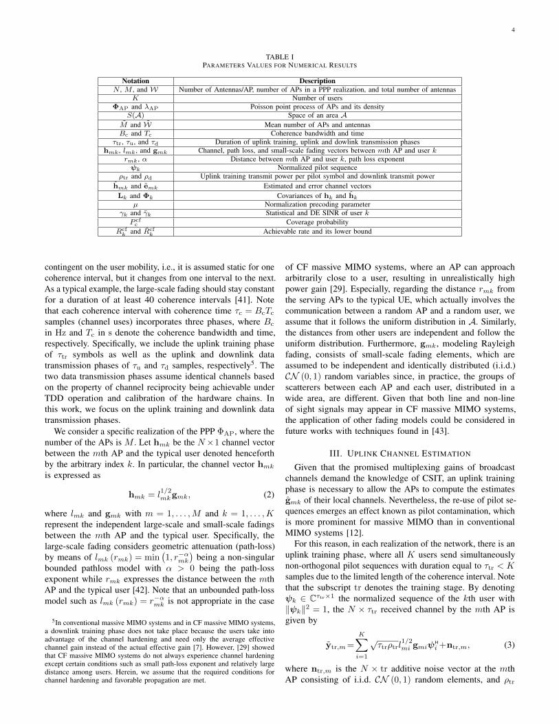
TABLE IPARAMETERS VALUES FOR NUMERICAL RESULTS
Notation DescriptionN , M , and W Number of Antennas/AP, number of APs in a PPP realization, and total number of antennas
K Number of usersΦAP and λAP Poisson point process of APs and its density
S(A) Space of an area AM and W Mean number of APs and antennasBc and Tc Coherence bandwidth and time
τtr, τu, and τd Duration of uplink training, uplink and dowlink transmission phaseshmk , lmk , and gmk Channel, path loss, and small-scale fading vectors between mth AP and user k
rmk , α Distance between mth AP and user k, path loss exponentψk Normalized pilot sequence
ρtr and ρd Uplink training transmit power per pilot symbol and downlink transmit powerhmk and emk Estimated and error channel vectorsLk and Φk Covariances of hk and hk
µ Normalization precoding parameterγk and γk Statistical and DE SINR of user kP cfc Coverage probability
Rcfk and Rcf
k Achievable rate and its lower bound
contingent on the user mobility, i.e., it is assumed static for onecoherence interval, but it changes from one interval to the next.As a typical example, the large-scale fading should stay constantfor a duration of at least 40 coherence intervals [41]. Notethat each coherence interval with coherence time τc = BcTc
samples (channel uses) incorporates three phases, where Bc
in Hz and Tc in s denote the coherence bandwidth and time,respectively. Specifically, we include the uplink training phaseof τtr symbols as well as the uplink and downlink datatransmission phases of τu and τd samples, respectively5. Thetwo data transmission phases assume identical channels basedon the property of channel reciprocity being achievable underTDD operation and calibration of the hardware chains. Inthis work, we focus on the uplink training and downlink datatransmission phases.
We consider a specific realization of the PPP ΦAP, where thenumber of the APs is M . Let hmk be the N×1 channel vectorbetween the mth AP and the typical user denoted henceforthby the arbitrary index k. In particular, the channel vector hmkis expressed as
hmk = l1/2mkgmk, (2)
where lmk and gmk with m = 1, . . . ,M and k = 1, . . . ,Krepresent the independent large-scale and small-scale fadingsbetween the mth AP and the typical user. Specifically, thelarge-scale fading considers geometric attenuation (path-loss)by means of lmk (rmk) = min
(1, r−αmk
)being a non-singular
bounded pathloss model with α > 0 being the path-lossexponent while rmk expresses the distance between the mthAP and the typical user [42]. Note that an unbounded path-lossmodel such as lmk (rmk) = r−αmk is not appropriate in the case
5In conventional massive MIMO systems and in CF massive MIMO systems,a downlink training phase does not take place because the users take intoadvantage of the channel hardening and need only the average effectivechannel gain instead of the actual effective gain [7]. However, [29] showedthat CF massive MIMO systems do not always experience channel hardeningexcept certain conditions such as small path-loss exponent and relatively largedistance among users. Herein, we assume that the required conditions forchannel hardening and favorable propagation are met.
of CF massive MIMO systems, where an AP can approacharbitrarily close to a user, resulting in unrealistically highpower gain [29]. Especially, regarding the distance rmk fromthe serving APs to the typical UE, which actually involves thecommunication between a random AP and a random user, weassume that it follows the uniform distribution in A. Similarly,the distances from other users are independent and follow theuniform distribution. Furthermore, gmk, modeling Rayleighfading, consists of small-scale fading elements, which areassumed to be independent and identically distributed (i.i.d.)CN (0, 1) random variables since, in practice, the groups ofscatterers between each AP and each user, distributed in awide area, are different. Given that both line and non-lineof sight signals may appear in CF massive MIMO systems,the application of other fading models could be considered infuture works with techniques found in [43].
III. UPLINK CHANNEL ESTIMATION
Given that the promised multiplexing gains of broadcastchannels demand the knowledge of CSIT, an uplink trainingphase is necessary to allow the APs to compute the estimatesgmk of their local channels. Nevertheless, the re-use of pilot se-quences emerges an effect known as pilot contamination, whichis more prominent for massive MIMO than in conventionalMIMO systems [12].
For this reason, in each realization of the network, there is anuplink training phase, where all K users send simultaneouslynon-orthogonal pilot sequences with duration equal to τtr < Ksamples due to the limited length of the coherence interval. Notethat the subscript tr denotes the training stage. By denotingψk ∈ Cτtr×1 the normalized sequence of the kth user with‖ψk‖2 = 1, the N × τtr received channel by the mth AP isgiven by
ytr,m=
K∑i=1
√τtrρtrl
1/2mi gmiψ
H
i +ntr,m, (3)
where ntr,m is the N × tr additive noise vector at the mthAP consisting of i.i.d. CN (0, 1) random elements, and ρtr
5
is the normalized signal-to-noise ratio (SNR). By assumingorthogonality among the pilot sequences, the mth AP estimatesthe channel by projecting ytr,mk onto 1√
τtrρtrψk, i.e., we have
ymk =1
√τtrρtr
ytr,mψk (4)
= gmkl1/2mk+
K∑i6=k
l1/2mi gmiψ
H
iψk+1
√τtrρtr
ntr,mψk, (5)
where the summation in the second term corresponds to themulti-user interference. Actually, this term is the source ofpilot contamination. Assuming, that the distance rmk is knowna priori, the mth AP obtains the linear minimum mean-squarederror (MMSE) estimate according to [44] as
hmk=E[hH
mkytr,mk](E[ytr,mky
H
tr,mk
])−1ymk
=lmk∑K
i=1 |ψHiψk|2lmi + 1
τtrρtr
ymk. (6)
Having obtained the estimated channel vector hmk, theestimation error vector, based on the orthogonality propertyof MMSE estimation, is written emk = hmk − hmk. Theestimated channel and estimation error vectors are uncorrelatedand Gaussian distributed with N identical elements havingzero mean and variances given by
σ2mk =
l2mkdm
(7)
and
σ2mk= lmk
(1− lmk
dm
), (8)
where dm =(∑K
i=1 |ψHiψk|2lmi + 1
τtrρtr
). Hence, we have
hmk ∈ CN×1 ∼ CN (0, lmkIN ), hmk ∈ CN×1 ∼CN
(0, σ2
mkIN)
and ek ∈ CN×1 ∼ CN(0, σ2
mkIN). At this
point, it is better for the sake of following algebraic manipu-lations to denote the vectors hk = [hT1k · · ·hTMk]T ∈ CW×1 ∼CN (0,Lk), hk = [hT1k · · · hTMk]T ∈ CW×1 ∼ CN (0,Φk)and ek ∈ CW×1 ∼ CN (0,Lk −Φk), where the matrices Lk,Φk = L2
kD−1, and D areW×W are block diagonal, i.e., Lk =
diag (l1kIN , . . . , lMkIN ), Φk = diag(σ2
1kIN , . . . , σ2MkIN
),
and D = diag (d1IN . . . , dMIN ), respectively. In addition,we denote Ck = Φ−1
k with Ck = diag (c1kIN , . . . , cMkIN ),where cmk = σ−2
mk.
IV. DOWNLINK TRANSMISSION
This section elaborates on the modeling and characterizationof the downlink transmission in one realization of the network,and aims at presenting the downlink SINR, when the APs arePPP distributed and apply conjugate beamforming while thesystem is impaired by pilot contamination. Having in mindthat the users are jointly served by the coordinated APs, wehighlight that the received signal by the typical user is givenby
yd,k =√ρd
∑i∈ΦAP
hH
i si + zd,k, (9)
where ρd is the downlink transmit power, hi is the N × 1channel vector between the associated AP located at xi ∈ R2
and the typical user including large and small-scale fadings,zd,k ∼ CN (0, 1) is the additive Gaussian noise at the kth user,and si denotes the transmitted signal from the ith AP.
Given that the number of PPP distributed APs in the areaA is M , we can rewrite (9) as
yd,k =√ρd
M∑m=1
hH
mksm + zd,k, (10)
where hmk is the channel between the mth AP and user k whilesm denotes the transmitted signal from the mth associated AP.The transmit signal is written as
sm =õ
K∑k=1
fmkqk (11)
with qk ∈ C being the transmit data symbol for the typicaluser satisfying E
[|qk|2
]= 1. Actually, the overall transmit
signal to users can be written in a vector notation as q =[q1, . . . , qK
]T ∈ CK ∼ CN (0, IK) for all users. Moreover,fmk represents the (m, k)th element of a linear precoder. Inorder to avoid sharing channel state information between theAPs, we assume scaled conjugate beamforming. We selectconjugate beamforming precoding because of its computationalefficiency and good performance in both massive MIMO andSCs designs [6], [7]. Thus, the expression of the precoderis fmk = cmkhmk. Regarding the scaling, it relies on astatistical channel inversion power-control policy that alsoeases the algebraic manipulations henceforth [45]. Also, µ isa normalization parameter obtained by means of the constraintof the transmit power E [ρdssH] = ρd. Hence, we have
µ =1
E [tr FmFHm], (12)
where Fm = [fm1 · · · fmK ] ∈ CN×K is the precoding matrix.Taking into account for the imperfect CSIT due to pilot
contamination (see (5)), the received signal by the typical user,given by (10), is written as
yd,k =√µρd
M∑m=1
K∑i=1
cmihH
mkhmiqi + zd,k (13)
=√µρdE
[hH
kCkhk
]qk +
√µρdhH
kCkhkqk
−√µρdE[hH
kCkhk
]qk +
√µρd
K∑i 6=k
hH
kCihiqi + zd,k, (14)
where the second and fourth terms in (14) describe the desiredsignal and the multi-user interference. Note that we use similartechniques to [46], i.e., (13) has been transformed to (14)for the derivation of the SINR provided below since theusers are not aware of the instantaneous CSI, but only ofits statistics which can be easily acquired, especially, if theychange over a long-time scale. Hence, user k has knowledgeof only E
[hH
kCkhk
]. In fact, similar to the well-established
bounding technique in [46], if we consider that (14) representsa single-input single-output (SISO) system, the effective SINRof the downlink transmission from all the APs to the typical
6
user under imperfect CSIT, conditioned on the distances ofAPs lmk for m = 1, . . . ,M , is given by
γk =
∣∣∣E [hH
kCkhk
] ∣∣∣2var[hH
kCkhk
]+∑Ki 6=k E
[∣∣∣hH
kCihi
∣∣∣2]+ 1µρd
, (15)
where we assume that the APs treat the unknown terms asuncorrelated additive noise. According to [7, Fig. 2], theachievable rate, given by (15), provides a rigorous bound closeto the achievable rate corresponding to the scenario where theusers know the instantaneous channel gain.
As specified by its concept, a CF massive MIMO networkcomprises a very large number of APs distributed across ageographic area. Hence, relied on the theory of DE analysiswhich is a common mathematical tool in the large MIMOliterature [37], [38], [47], we can apply it in the proposedCF massive MIMO system, and obtain the asymptotic SINRconditioned on the distances of APs as K, W → ∞, whilethe finite ratio K/W is kept constant. Actually, the definitionof DEs, first met in [47] follows.
Definition 1 (Deterministic Equivalent [47]): The deter-ministic equivalent of a sequence of random complex values(Xn)n≥1 is a deterministic sequence
(Xn
)n≥1
, which approx-imates Xn such that
Xn − Xna.s.−−−−→n→∞
0, (16)
where a.s.−−−−→n→∞
0 is taken to mean almost sure convergence.As far as the authors are aware, the DE analysis is applied
for the first time in the area of CF massive MIMO. Remarkably,the literature and the simulations in Section VII exhibit thatthe proposed result is of high practical value because of tworeasons. First, the result is tight even for conventional systemdimensions, i.e., when 20 APs serve 10 users. The secondreason lies in the fact that a statistical description of the SINRis intractable because of i) the different path-losses from thedifferent APs constituting the desired signal, ii) the cross-products of the path-losses from the different interferers inthe denominator can be correlated with the numerator becausethey contain common path-loss terms.
Conditioned on the distances of APs, the deterministic SINRγk, obtained such that γk − γk
a.s.−−−−→M→∞
0, is provided below.Proposition 1: Given a realization of ΦAP and conditioned
on the APs distances, the deterministic SINR of the downlinktransmission from the PPP distributed APs to the typical user ina CF massive MIMO system, accounting for pilot contaminationand conjugate beamforming, is given by
γk �W
1W∑Ki=1 tr DL−2
i
(Lk + W
ρd
)− 1
. (17)
Proof: See Appendix A.Note that (17) holds for any given realization of ΦAP. In
other words, this SINR hides the randomness regarding theAP locations, which is found at the path-losses between theAPs and the users. Hence, in order to study the impact of APdensity, we have to derive its expectation with respect to thedistances. Specifcally, M is found in both W and inside the
trace as one could see in the element-wise expression givenby 32. By taking the expectation and applying [48, Lemma 1],we have
γk �E [M ]N
E[
1M
∑Ki=1
∑Mm=1 dml
−2mi
(lmk + MN
ρd
)− 1] . (18)
Following a procedure as in Appendix B, we result in thatγk does not depend on the AP density. This property isknown as SINR invariance and holds for single-slope pathloss models [49].
Regarding the other primary system parameters, γk in 17saturates with increasing the number of antennas per AP N .Also, when ρd →∞, i.e., in the high SNR regime, the SINRreaches a ceiling. Moreover, the SINR decreases with K andwith the severity of pilot contamination.
V. COVERAGE PROBABILITY
The focal point of this section is to shed light on thecoverage potentials of CF massive MIMO systems in therealistic setting where the APs are randomly located. Giventhat the coverage probability of such a system has not beenpresented before, the first task is to provide a formal definition.The next step is the presentation of the result bringing onthe surface its dependence on the system parameters. Thederivation, provided in Appendix B, encompasses techniquesand tools from stochastic geometry. Notably, we result in thefirst expression in the literature that describes the coverageprobability of a CF massive MIMO system, being actually thecomplementary cumulative distribution function (CCDF) of theSINR.
Definition 2 ([15], [34]): A typical user is in coverage ina CF massive MIMO system if the downlink SINR from therandomly located APs in the network is higher than the targetSINR T .
Theorem 1: The downlink coverage probability of a pilotcontaminated CF massive MIMO network, where the APs arePPP distributed and undergo a single-slope path loss modelwhile employing conjugate beamforming, is lower boundedby (19), or equivalently (20) shown at the top of next page,
where W = E [W] and η = W(W!)− 1W .
Proof: See Appendix B.Focusing on (20), we observe better the dependence of the
coverage probabilty from the system parameters. In particular,we notice the decrease of P cf
c with K being the number ofusers. Also, the more severe the pilot contamination is, thelower the coverage probability becomes. A similar behaviorresults by increasing the target SINR T . In fact, if T →∞, thecoverage probability becomes zero. In addition, if the path-lossexponent α > 2 increases, P cf
c decreases as expected. Also,in the high SNR regime (ρd →∞), the coverage probabilitysaturates which means that it is interference limited while whenρd → 0 it is noise limited since P cf
c → 0. Furthermore, thedependence from the AP density and the number of antennasper AP is given indirectly by means of W . However, thecoverage probability is a complicated function of W and thedependence from the corresponding parameter can be shownonly by means of numerical results. In Sec. VII, it is depicted
7
P cfc ≥
W∑n=1
(Wn
)(−1)
n+1e−nηT
(K
απρd
(∑Kj=1 |ψ
Hjψk|
2(αρd+W(α−2))+(α−2)ρd+W(α−1)
τtrρtr
)−1)
(19)
= 1−(
1− e−ηT(
Kαπρd
(∑Kj=1 |ψ
Hjψk|
2(αρd+W(α−2))+(α−2)ρd+W(α−1)
τtrρtr
)−1))W
. (20)
that P cfc increases with λAP and saturates when the AP density
becomes large. This saturation is appeared in SCs too [49] inthe case of single-slope path loss models. A similar behavioris observed regarding the number of antennas per AP.
VI. ACHIEVABLE RATE
Herein, we provide a closed-form expression of the downlinkachievable rate in a CF massive MIMO system. Specifically,the following lemma allows to obtain a tractable lower boundfor a large number of APs.
Lemma 1 ( [11]): The downlink ergodic channel capacityof the typical user k in a CF massive MIMO system withconjugate beamforming, PPP distributed AP, and a single-slopepath loss model is lower bounded by the average achievablerate given by
Rcfk =
(1− τtr
τc
)E [log2 (1 + γk)] b/s/Hz, (21)
where τc is the channel coherence interval in number of samples,τtr is the duration of the uplink training phase, and γk is givenby (17).
Given that the terms in γk are actually averaged over thesmall-scale fading, the expectation in the previous lemmaapplies to the remaining statistical variables, which are theAP distances. Regarding the pre-log factor, it concerns thepilot overhead. In order to avoid intractable lengthy numericalevaluations of the integrals with respect to the AP distances, weapply Jensen’s inequality. The following proposition presentsa closed-form expression for the downlink achievable Rk.
Theorem 2: A lower bound of the downlink averageachievable rate per user with conjugate beamforming in a CFmassive MIMO system with PPP distributed APs is expressedby
Rcfk =
(1− τtr
τc
)log2 (1 + γk) b/s/Hz, (22)
where γk is obtained as shown in (23) at the top of the nextpage.
Proof: See Appendix C.Basically, the impact of the system parameters on the
achievable rate is shown by means of γk. Hence, given that γkdecreases with the number of users K and pilot contaminationas can be seen by (23), the corresponding rate decreases aswell. Moreover, the achievable rate increases with the numberof antennas per AP N , the AP density λAP, and the transmitpower. However, the rate saturates when the number of antennasper AP N becomes large as expected. In addition, we notice aceiling at the rate at high ρd but it keeps increasing with theAP density. A similar behavior regarding the AP density is metin small cell systems [49] when a single-slope path loss model
is considered. Moreover, the rate decreases with the path-lossexponent α.
VII. NUMERICAL RESULTS
In this section, we illustrate and discuss the behavior ofPPP located APs in a CF architecture for the first time in thecorresponding literature since prior works have not taken intoaccount a realistic and well-accepted model for the randomnessof APs positions in the analysis. We focus on the analyticalexpressions concerning the coverage probability P cf
c and theachievable rate Rcf
k , which are provided by means of Theorem 1and Theorem 26.
For the sake of comparison, we consider the system modelin [15], where independent users are associated with theirnearest multi-antenna AP, while the remaining APs act asinterferers. Henceforth, we refer to this scenario as “smallcells” or “SCs”. Especially, we assume that the base stationsin that model have the same number of antennas serving asingle user, i.e., in [15], we set M = 4 and K = 1 whilethe imperfect CSIT model in that scenario is replaced by thecurrent one. In addition, we assume no hardware impairmentsand channel aging. In addition, similar to [7], we assume thathandovers among the APs do not take place.
One main difference with CF massive MIMO is that, inSCs, the effective channel power does not harden while inthe case of CF massive MIMO systems, the signal powertends to its mean as the number of APs becomes large [7]. Inother words, SCs need to estimate their effective channel gain.Hence, SCs require both uplink and downlink training phaseswhile CF massive MIMO systems rely only on uplink training.During the investigation of their performance, this differencewill be more obvious. Moreover, an additional advantage, metin CF massive MIMO, is favorable propagation which canachieve optimal performance with simple linear processing.For example, on the uplink, the noise and interference canbe almost canceled out with a simple linear detector suchas the matched filter. Another primary reason justifying theoutperformance of CF massive MIMO systems against SCs isthat the latter have inherent the inter-cell interference while CFsystems implement co-processing and all the APs that affect aspecific user take into account for its interference. As a result,the CF approach achieves to suppress inter-cell interference byeliminating any cell boundaries [30].
6It is worthwhile to mention that both theorems are obtained based ona single-slope path loss model but they could also be easily generalized todescribe more general path-loss models such as the multi-slope path lossmodel used in the seminal work regarding CF massive MIMO systems [7]. Infact, this is the topic of ongoing work by the authors, i.e., the analysis andcomparison of multi-slope path loss models in CF massive MIMO systems.
8
γk = λAPN
K
απρd
K∑j=1
|ψH
jψk|2 (αρd +N (α− 2)) +(α− 2) ρd +N (α− 1)
τtrρtr
− 1
−1
. (23)
TABLE IIPARAMETERS VALUES FOR NUMERICAL RESULTS
Description ValuesNumber users K = 10
Number of Antennas/AP N = 5AP density λAP = 40 APs/km2
Communication bandwidth, carrier frequency Wc = 20 MHz, f0 = 1.9 GHzUplink training transmit power per pilot symbol ρtr = 100 mW
Downlink transmit power ρd = 200 mWPath loss exponent α = 3.5
Coherence bandwidth and time Bc = 200 KHz and Tc = 1 msDuration of uplink training τtr = 10 samples
Duration of uplink and downlink training is SCs τtr = τd = 10 samplesBoltzmann constant κB = 1.381× 10⁻²³ J/KNoise temperature T0 = 290 K
Noise figure NF = 9 dB
A set of Monte Carlo simulations verifies the analyticalexpressions. In fact, by plotting the proposed analytical expres-sions along with the simulated results represented by meansof black bullets, we observe their coincidence7. Especially, thesimulated results are generated by means of the correspondingstatistical SINR given by (15) by averaging over 104 randominstances of the channels while the coverage probability andachievable rate are obtained as an average of 104 realizationsof different random AP topologies. The results correspondingto CF massive MIMO systems and SCs are depicted by meansof “solid” blue and “dot” red lines, respectively.
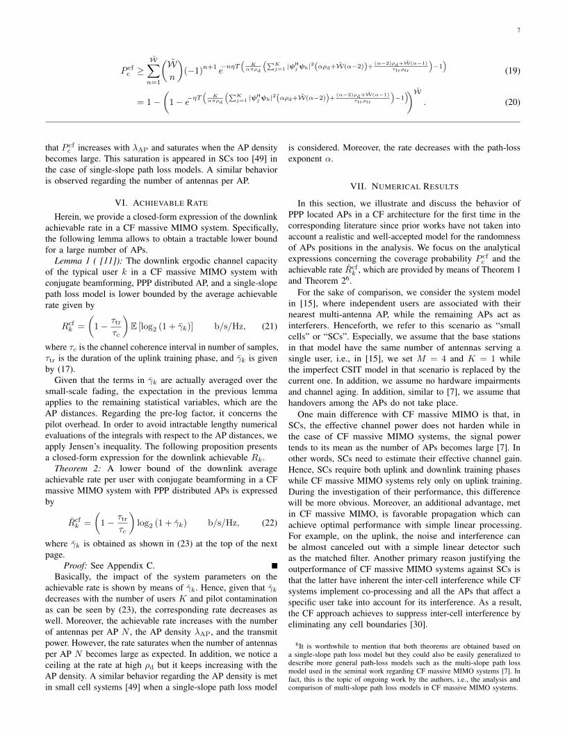
Fig. 1. Coverage probability for varying AP density λAP versus the targetSINR T for both CF massive MIMO systems and SCs.
7In particular, the fact that the analytical results, obtained by means of theDE analysis, coincide with the simulations means that the former can be usedas tight approximations in the case of a CF massive MIMO system. Althoughthis is a known result in the massive MIMO literature [37], [50], the DEanalysis has not been verified before as an RMT tool for CF massive MIMOsystems.
A. Setup
We choose a finite window of area of 1 km× 1 km, wherewe distribute the APs, each having N = 5 antennas, accordingto a PPP realization with density λAP = 40 APs/km2 unlessotherwise stated. Given that the analytical expressions relyon the assumption of an infinite plane while the simulationconsiders a finite square, we assume that this area is wrappedaround at the edges to prevent any boundary effects. In addition,the structure of the system includes a number of APs servingsimiltaneously K = 10 randomly distributed users. Actually,similar to [7], we use the default values in Table II unlessotherwise stated. The normalized uplink training transmit powerper pilot symbol ρtr and downlink transmit power ρd resultby dividing ρtr and pd by the noise power NP given in W byNP = Wc × κB × T0 × NF, where the various parameters arefound in Table II. Also, in order to guarantee a fair comparisonbetween CF massive MIMO systems and SCs, the total radiatedpower must be equal in both architectures. Hence, we havethat ρsc
tr = ρtr and pscd = M
K pd, where ρsctr and pd
sc are thenormalized uplink training and downlink transmit powers [7].
B. Depictions and Discussions
1) Coverage Probability: The coverage probability, describ-ing the SCs setting, is denoted by P sc
c and provided by [15,Th. 1].
In Fig. 1, we assess the performance of the proposed boundby varying the target SINR. Specifically, firstly, it is shownthe tightness of the proposed bound against the SINR. It isevident that the tightness is very good, however, it is relaxedas λAP increases. Although someone would expect that thebound would become tighter with M ∼ λAP due to theuse of the DE analysis, this contradiction appears due tothe Alzer’s inequality. Next, Fig. 1 depicts that the coverageprobability decreases with the target SINR in both cases ofCF massive MIMO and SCs because of the inter-user andinter-cell interferences, respectively. Notably, the estimation
9
error has its own contribution. In other words, these reasons,degrading the SINR, result in less coverage as the thresholdincreases. Especially, when the target SINR tends to zero,the coverage probability becomes one, when T → ∞, thecoverage probability approaches zero, while, in practice, fortypical values of T being around 15 dB, P sc
c is finite anddecreases. It is obvious that CF massive MIMO systems, unlikeSCs, systematically provide higher coverage for all values ofthe target SINR T because they take benefit from favorablepropagation, channel hardening, and suppression of the inter-cell interference. Actually, as the AP density λAP increases,these effects contribute more to the outperformance of CFmassive MIMO systems against SCs having a cellular nature.
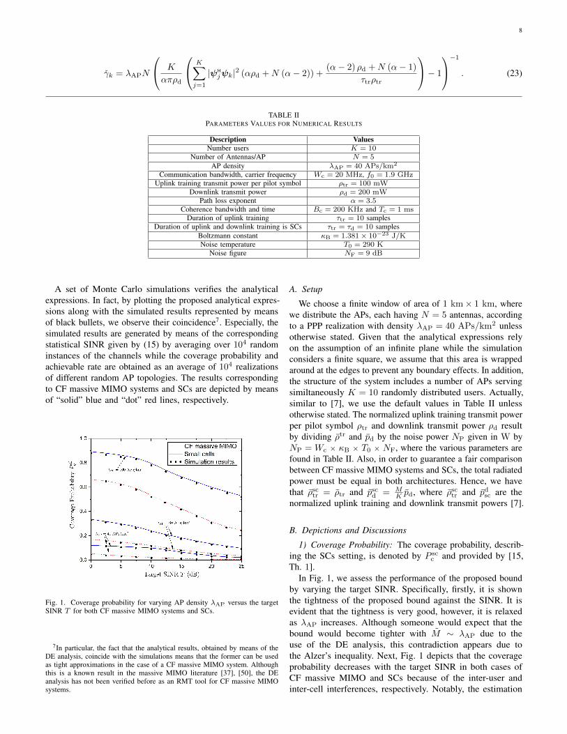
Fig. 2. Coverage probability for varying target SINR T versus the AP densityλAP for both CF massive MIMO systems and SCs.
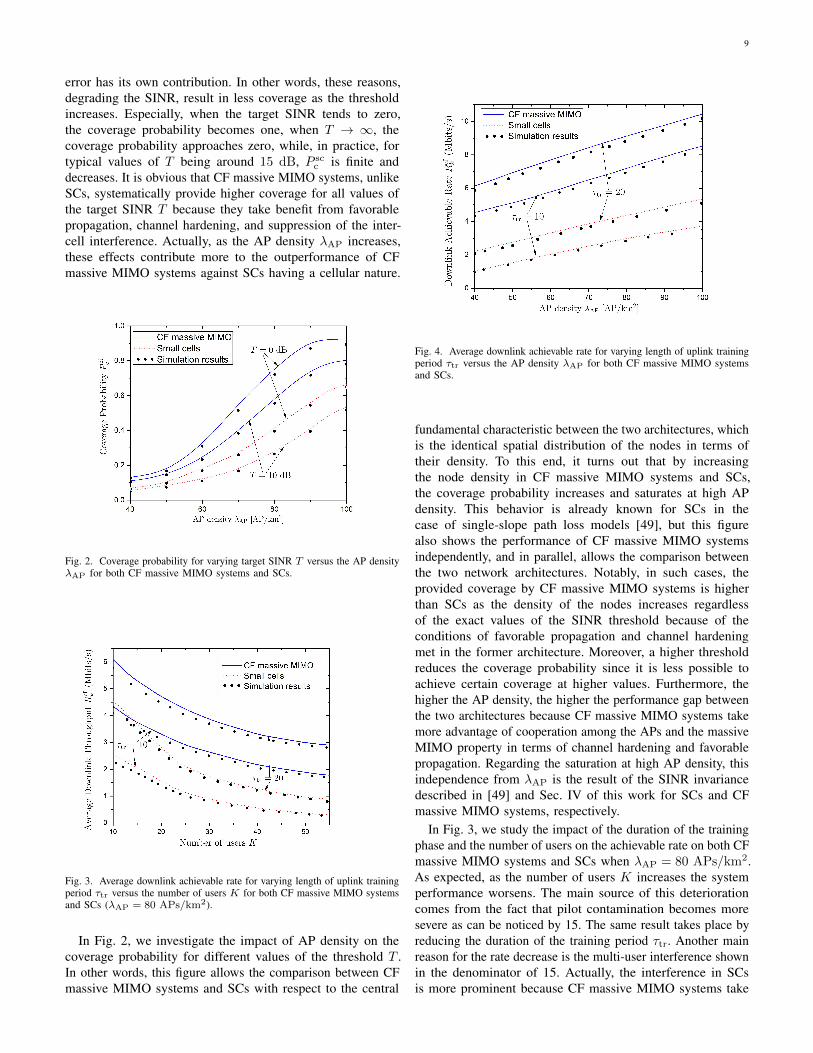
Fig. 3. Average downlink achievable rate for varying length of uplink trainingperiod τtr versus the number of users K for both CF massive MIMO systemsand SCs (λAP = 80 APs/km2).
In Fig. 2, we investigate the impact of AP density on thecoverage probability for different values of the threshold T .In other words, this figure allows the comparison between CFmassive MIMO systems and SCs with respect to the central
Fig. 4. Average downlink achievable rate for varying length of uplink trainingperiod τtr versus the AP density λAP for both CF massive MIMO systemsand SCs.
fundamental characteristic between the two architectures, whichis the identical spatial distribution of the nodes in terms oftheir density. To this end, it turns out that by increasingthe node density in CF massive MIMO systems and SCs,the coverage probability increases and saturates at high APdensity. This behavior is already known for SCs in thecase of single-slope path loss models [49], but this figurealso shows the performance of CF massive MIMO systemsindependently, and in parallel, allows the comparison betweenthe two network architectures. Notably, in such cases, theprovided coverage by CF massive MIMO systems is higherthan SCs as the density of the nodes increases regardlessof the exact values of the SINR threshold because of theconditions of favorable propagation and channel hardeningmet in the former architecture. Moreover, a higher thresholdreduces the coverage probability since it is less possible toachieve certain coverage at higher values. Furthermore, thehigher the AP density, the higher the performance gap betweenthe two architectures because CF massive MIMO systems takemore advantage of cooperation among the APs and the massiveMIMO property in terms of channel hardening and favorablepropagation. Regarding the saturation at high AP density, thisindependence from λAP is the result of the SINR invariancedescribed in [49] and Sec. IV of this work for SCs and CFmassive MIMO systems, respectively.
In Fig. 3, we study the impact of the duration of the trainingphase and the number of users on the achievable rate on both CFmassive MIMO systems and SCs when λAP = 80 APs/km2.As expected, as the number of users K increases the systemperformance worsens. The main source of this deteriorationcomes from the fact that pilot contamination becomes moresevere as can be noticed by 15. The same result takes place byreducing the duration of the training period τtr. Another mainreason for the rate decrease is the multi-user interference shownin the denominator of 15. Actually, the interference in SCsis more prominent because CF massive MIMO systems take
10
advantage of the favorable propagation. Relied on this property,we observe that for a given training period the gap betweenCF and SC systems increases with K, since the interferenceincreases. In addition, by increasing the interference, i.e., whenK grows, CF massive MIMO systems perform better thanSCs because the former enjoys cooperative multipoint jointprocessing which is more robust at higher interference. Hence,in the case that τtr = 20 samples, the gap between CF andSCs increases from 1.6 Mbits/s to 2.1 Mbits/s when K = 10and K = 55, respectively.
Fig. 4 shows the achievable rate against the AP density inthe cases of both CF massive MIMO and SC systems. Byincreasing τtr, the estimated channel is improved in all casesdue to less pilot contamination, and thus, the rate increases.Moreover, as anticipated, an increase in λAP increases the rateas also described in Sec. VI, which agrees with the behaviorof single-slope path loss models in SCs [49]. Actually, the ratein both CF massive systems and SCs increases with increasingthe mean number of APs due to the array gain and diversitygain, respectively, as mentioned in [7]. However, CF massiveMIMO systems present a higher rate for several reasons. Inparticular, CF massive MIMO systems perform much betterthan SCs with increasing λAP because they take advantage ofthe achievable favorable propagation and channel hardening.Furthermore, as the AP density increases, the rate of CF systemsis higher because the benefit from the cooperation among theAPs increases. Nevertheless, the gap between the CF linesincreases since the advantage from the AP cooperation increasesby exploiting better the interference corresponding to a certainduration of the training phase. This property is basicallyjustified by the reduction of the impact of pilot contaminationas τtr increases. In other words, CF massive MIMO systems aremore robust against pilot contamination as the mean numberof APs increases. Hence, when λAP = 40 APs/km2, the gapis almost 1.6 Mbits/s while when λAP = 100 APs/km2, thegap has increased to almost 2 Mbits/s. At these differencesof AP density, the gap is not such big but it becomes biggerwhen more APs are employed.
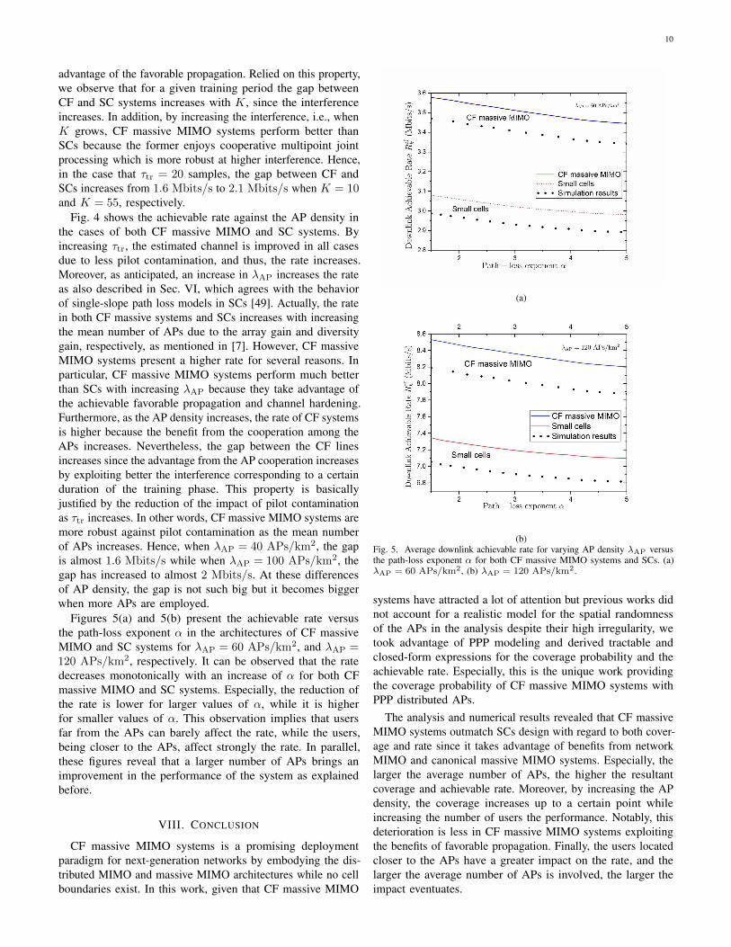
Figures 5(a) and 5(b) present the achievable rate versusthe path-loss exponent α in the architectures of CF massiveMIMO and SC systems for λAP = 60 APs/km2, and λAP =120 APs/km2, respectively. It can be observed that the ratedecreases monotonically with an increase of α for both CFmassive MIMO and SC systems. Especially, the reduction ofthe rate is lower for larger values of α, while it is higherfor smaller values of α. This observation implies that usersfar from the APs can barely affect the rate, while the users,being closer to the APs, affect strongly the rate. In parallel,these figures reveal that a larger number of APs brings animprovement in the performance of the system as explainedbefore.
VIII. CONCLUSION
CF massive MIMO systems is a promising deploymentparadigm for next-generation networks by embodying the dis-tributed MIMO and massive MIMO architectures while no cellboundaries exist. In this work, given that CF massive MIMO
(a)
(b)Fig. 5. Average downlink achievable rate for varying AP density λAP versusthe path-loss exponent α for both CF massive MIMO systems and SCs. (a)λAP = 60 APs/km2, (b) λAP = 120 APs/km2.
systems have attracted a lot of attention but previous works didnot account for a realistic model for the spatial randomnessof the APs in the analysis despite their high irregularity, wetook advantage of PPP modeling and derived tractable andclosed-form expressions for the coverage probability and theachievable rate. Especially, this is the unique work providingthe coverage probability of CF massive MIMO systems withPPP distributed APs.
The analysis and numerical results revealed that CF massiveMIMO systems outmatch SCs design with regard to both cover-age and rate since it takes advantage of benefits from networkMIMO and canonical massive MIMO systems. Especially, thelarger the average number of APs, the higher the resultantcoverage and achievable rate. Moreover, by increasing the APdensity, the coverage increases up to a certain point whileincreasing the number of users the performance. Notably, thisdeterioration is less in CF massive MIMO systems exploitingthe benefits of favorable propagation. Finally, the users locatedcloser to the APs have a greater impact on the rate, and thelarger the average number of APs is involved, the larger theimpact eventuates.
11
APPENDIX APROOF OF PROPOSITION 1
We divide each term of (15) by the number W raised to 2,in order to derive the correspondsing DEs. Starting with thedesired signal power, we have
Sk =µ
W2
∣∣∣E [hH
kCkhk
]∣∣∣2. (24)
First, the normalization parameter can be written by meansof (12) and the expression of MRT precoding as
µ =1
1WE
[∑Ki=1 hH
iC2i hi
]�
(1
W
K∑i=1
tr C2iΦi
)−1
=
(1
W
K∑i=1
tr Ci
)−1
= µ, (25)
where we have applied [37, Thm. 3.7]8. Note that H =[h1, . . . ,hK
]∈ CW×K is the channel matrix from the APs to
all users. The DE of (24) is obtained as
1
WE[hH
kCkhk
]=
1
WE[(
hH
k+eH
k
)Ckhk
](26)
=1
WE[hH
kCkhk
]� 1
Wtr CkΦk
= 1, (27)
where in (26) we have taken into account that gk and ek areuncorrelated, and next we have applied [37, Thm. 3.7] sinceall conditions are satisfied. Note that the matrices commutebecause they are diagonal. Therefore, the DE signal powerSk = limW→∞ Sk is written as
Sk = µ. (28)
This result verifies the chosen scaling regarding the precoder.Next, we focus on the derivation of DEs of the denominatorterms. The first term, involving the variance, is obtained as
1
W2var[hH
kCkhk
]− 1
W2E[∣∣∣eH
kCkhk
∣∣∣2] a.s.−−−−→W→∞
0. (29)
In (29), we have exploited the property of the variance operatorvar [x] = E[x2]−E2[x] and that ek = hk−hk. In addition, wehave applied [37, Thm. 3.7]. After applying again this theorem,we have
1
W2E[∣∣∣eH
kCkhk
∣∣∣2] � 1
W2tr C2
kΦk (Lk −Φk)
=1
W2tr(DL−1
k − IW). (30)
8Given two infinite sequences an and bn, the relation an � bn is equivalentto an − bn
a.s.−−−−→n→∞
0.
The final term becomes
1
W2E[∣∣∣hH
kCihi
∣∣∣2] � 1
W2tr C2
iΦiLk
=1
W2tr DL−2
i Lk (31)
since hk and hi are mutually independent. Taking intoaccount that the SINR is conditioned on Lk, substitutionof (25), (28), (30), and (31) into (15) completes the proof.
APPENDIX BPROOF OF THEOREM 1
The proof starts by writing the terms of (17), includingthe block matrix traces, as summations over the diagonalelements (element-wise). Thus, the DE SINR, conditionedon the distances rmi for i = 1, . . . ,K, is obtained as
γk �MN
1M
∑Ki=1
∑Mm=1 dml
−2mi
(lmk + MN
ρd
)− 1
. (32)
We continue with the derivation of distribution of the SINR,conditioned on a realization of lmi for i = 1, . . . ,K, i.e.,P(γk > T |lm1, . . . , lmK). Specifically, after substituting (32)inside the expression of the coverage probability, and by meansof several algebraic manipulations, we obtain (33). Hence, theconditional coverage probability is written as shown at the topof next page
In (34), we have approximated the constant number Wby considering the dummy gamma variable g, having meanW = MN and shape parameter W = E [W ] = MN . Thisapproximation becomes tighter as W goes to infinity [51],since limy→∞
yyxy−1e−yx
Γ(y) = δ (x− 1) with δ (x) being Dirac’sdelta function. Notably, this approximation, used in [52],becomes more precise in our system model involving a largenumber (massive) of APs. Note that the precision increasesas the number of antennas per AP increases. In (35), wehave applied Alzer’s inequality (see [51, Lemma 1]), where
η = W(W!)− 1W , while afterwards, we have used the
Binomial theorem. Note that (35) does not contain any randomvariable since this expression is conditioned on the distances.Next, the coverage probability is obtained by evaluating theexpectation of (36) with respect to AP locations given thatthe distances between the APs and the users are uniformlydistributed. Thus, we have
P cfc =
W∑n=1
(Wn
)(−1)
n+1
× E
[exp
(− nηT
(1
M
K∑i=1
M∑m=1
Imk − 1
))](37)
≥W∑n=1
(Wn
)(−1)
n+1enηTλAP
× exp
(− nηT E
[1
M
K∑i=1
M∑m=1
Imk
]), (38)
12
P (γk >T |rm1, . . . , rmK)= P
(W> T
(1
M
K∑i=1
M∑m=1
dml−2mi
(lmk +
MN
ρd
)− 1
))(33)
≈ P
(g> T
(1
M
K∑i=1
M∑m=1
dml−2mi
(lmk +
MN
ρd
)− 1
))(34)
≈ 1−
(1− exp
(− ηT
(1
M
K∑i=1
M∑m=1
dml−2mi
(lmk +
MN
ρd
)− 1
)))W(35)
=
W∑n=1
(Wn
)(−1)
n+1exp
(− nηT
(1
M
K∑i=1
M∑m=1
dml−2mi
(lmk +
MN
ρd
)− 1
)). (36)
where we have set Imk = dml−2mi
(lmk + MN
ρd
)and have
applied Jensen’s inequality since exp (·) is a convex function.By focusing on the derivation of the expectation, we have
limR→∞
E
[1
M
K∑i=1
M∑m=1
Imk
]
= limR→∞
EM
E|M 1
M
K∑i=1
M∑m∈ΦAP∩B(o,R)
Imk|M = Φ(B (o,R))
(39)
=
K∑i=1
limR→∞
EM [Imk] (40)
=
K∑i=1
E
K∑j=1
|ψH
jψk|2lmj +1
τtrρtr
(lmk +E[M ]N
ρd
)l−2mi
(41)
where in (39), we have assumed a ball of radius R centered atthe origin that contains M = Φ (B(o,R)) points with S(A) =|B(o,R)|. By conditioning on this area of radius R and on thenumber of points in this area, M in the denominator cancelsout with the number of points inside the ball. In (41), we havesubstituted Imk = dml
−2mi
(lmk + MN
ρd
)and dm. Then, we
substitute dm, and we result in
I1 =E
K∑i=1
K∑j=1
|ψH
jψk|2lmj +1
τtrρtr
l−2mi lmk
=E
K∑i=1
K∑j=1
|ψH
jψk|2lmj l−2mi lmk
+1
τtrρtrE
[K∑i=1
l−2mi lmk
](42)
and
I2 =λAPN
ρdE
K∑i=1
K∑j=1
|ψH
jψk|2lmj +1
τtrρtr
l−2mi
.(43)
Regarding the first part of (42), we have
E
K∑i=1
K∑j=1
|ψH
jψk|2lmj l−2mi lmk
=
∑Ki=1 |ψH
iψk|2E[l−1mi lmk
]if j = i∑K
i=1 E[l−2mi l
2mk
]if j = k∑K
j 6=i,k |ψHjψk|2E
[lmj l
−2mi lmk
]otherwise
. (44)
The expectation in the first branch of the right hand side of (44)for i 6= k gives
E[l−1mi lmk
]≥ 1
E [lmi]E [lmk] (45)
= 1, (46)
where (45) takes advantage of Jensen’s inequality, and then, (46)is obtained since the two variables have the same marginaldistribution. By following similar steps, the derivation of theexpectation in the second branch is straightforward, while thelast branch becomes
E[lmj l
−2mi lmk
]=
{E[lmj l
−1mk
]if i = k
E[lmj l
−2mi lmk
]if i 6= k
. (47)
If i = k, the expression in the first branch is identical to (45),and the result is the same. The remaining term in (47) is writtenas
E[lmj l
−2mi lmk
]= E
[lmj]E[l−2mi
]E [lmk] (48)
≥ E[lmj]E[l−1mi
]2 E [lmk] (49)
≥ 1, (50)
where (48) considers the independence among the variables,while (49) exploits the inequality E
[x2]≥ E [x]
2. Last, (50)follows basically the same steps as those taken in (46). Thesecond part of (42) becomes
E
[K∑i=1
l−2mi lmk
]=
{E[l−1mi
]if i = k∑K
i 6=k E[l−2mi lmk
]if i 6= k
. (51)
Let us now tackle both expectations separately. The former,i.e., E
[l−vmi]
for v = 1 results in
E[l−vmi]
= E[
1
lvmi
](52)
≥ 1
E [lvmi], (53)
13
where Jensen’s inequality has been applied in (52). The finalexpression is obtained by computing E [lvmi] as
E [lvmi] = 2π
(∫ 1
0
ydy +
∫ ∞1
y−va+1dy
)(54)
=vαπ
vα− 2. (55)
The latter expectation in (51) is computed as
E[l−2mi lmk
]= E
[l−2mi
]E [lmk] (56)
≥ E[l−1mi
]2 E [lmk] (57)
≥ E [lmk]
E [lmi]2 (58)
=1
E [lmi](59)
=α− 2
απ, (60)
where we have used similar techniques as before. By substitut-ing all these expressions in (42), we obtain I1. Similarly, I2
is obtained as
I2 =KλAPN
ρdαπ
K∑j=1
|ψH
jψk|2 (α− 2) +α− 1
τtrρtr
. (61)
Having derived I1 and I2, we substitute their expressionsin (41), and we eventually complete the proof resulting firstin (19), and next, in (37) after using the binomial theorem.
APPENDIX CPROOF OF THEOREM 2
The proof is split in two subsections. In the first subsection,we provide a more tractable bound than (21) that will allow toaverage over a PPP realization of the APs, while the secondsubsection includes the derivation of the PPP averaged inverseSINR.
A. Lower bound of the downlink SE
Rewriting (21) by means of the inverse of γk, and applyingthe Jensen inequality we have
E[log2
(1 +
1
γ−1k
)]≥ log2 (1 + γk) , (62)
where the expectation applies directly to the inverse of theSINR since γk = 1
E[γ−1k ]
.
B. Derivation of γkAfter writing the trace of each matrix as the sum of its entry-
wise elements, the expectation of the inverse of the SINR, givenby (32), is written as
E[γ−1k
]=
1
NE
[1
M2
(K∑i=1
M∑m=1
Imk −M
)]. (63)
We are going to compute the expectation by considering a ballof radius R centered at the origin including M = Φ (B (o,R))points with S(A) = |B (o,R) |. Then, conditioning on this
area of radius R and on the number of points in this finite area,the application of the law of large numbers will take place.In the next step, we remove the conditioning regarding thenumber of points while we let R→∞, i.e., the area goes toinfinity. Specifically, the expectation in the previous expressionbecomes
E
[1
M2
(K∑i=1
∑m∈ΦAP
Imk −M
)](64)
= limR→∞
E
1
M2
K∑i=1
∑m∈ΦAP∩B(o,R)
Imk −M
(65)
= limR→∞
EM[E|M
1
M2
K∑i=1
∑m∈ΦAP∩B(o,R)
Imk|M = Φ(B (o,R))
− 1
M
](66)
≈ limR→∞
1
EM [M ]E
[K∑i=1
l−2mi
K∑j=1
|ψH
jψk|2lmj+1
τtrρtr
lmk+N
ρd
K∑i=1
l−2mi
K∑j=1
|ψH
jψk|2lmj+1
τtrρtr
]− 1
EM [M ], (67)
where in (65), we have written the previous equation in termsof the ball of radius R. In (66), we condition on the numberof points inside the ball. Then, given that the SINR has beenderived by means of the DE analysis, which holds for M →∞,we are able to apply [48, Lemma 1]. Thus, in (67), we haveapplied this lemma. Next, we have EM [M ] = λAP|B (o,R) |while the other expectations in (67) have already been derivedin parts in Appendix B. Hence, γk is obtained, and the proofis concluded.
REFERENCES
[1] M. Shafi et al., “5G: A tutorial overview of standards, trials, challenges,deployment, and practice,” IEEE J. Sel. Areas Commun., vol. 35, no. 6,pp. 1201–1221, 2017.
[2] J. G. Andrews et al., “What will 5G be?” IEEE J. Sel. Areas Commun.,vol. 32, no. 6, pp. 1065–1082, 2014.
[3] A. Ericsson, “Ericsson mobility report: On the pulse of the networkedsociety,” Ericsson, Sweden, Tech. Rep. EAB-14, vol. 61078, 2015.
[4] E. Bastug et al., “Toward interconnected virtual reality: Opportunities,challenges, and enablers,” IEEE Commun. Mag., vol. 55, no. 6, pp.110–117, 2017.
[5] C. Wang et al., “A survey of 5G channel measurements and models,” IEEECommun. Surveys Tuts., vol. 20, no. 4, pp. 3142–3168, Fourthquarter2018.
[6] E. Larsson et al., “Massive MIMO for next generation wireless systems,”IEEE Commun. Mag., vol. 52, no. 2, pp. 186–195, February 2014.
[7] H. Q. Ngo et al., “Cell-free massive MIMO versus small cells,” IEEETrans. Wireless Commun., vol. 16, no. 3, pp. 1834–1850, 2017.
[8] H. Q. Ngo, E. Larsson, and T. Marzetta, “Energy and spectral efficiencyof very large multiuser MIMO systems,” IEEE Trans. Commun., vol. 61,no. 4, pp. 1436–1449, April 2013.
[9] H. Q. Ngo and E. G. Larsson, “No downlink pilots are needed in TDDmassive MIMO,” IEEE Trans.Wireless Commun., vol. 16, no. 5, pp.2921–2935, 2017.
[10] H. Q. Ngo, E. G. Larsson, and T. L. Marzetta, “Aspects of favorablepropagation in massive MIMO,” in 22nd European Signal ProcessingConference (EUSIPCO). IEEE, 2014, pp. 76–80.
[11] J. Hoydis, S. ten Brink, and M. Debbah, “Massive MIMO in the UL/DLof cellular networks: How many antennas do we need?” IEEE J. Select.Areas Commun., vol. 31, no. 2, pp. 160–171, February 2013.

14
[12] T. Marzetta, “Noncooperative cellular wireless with unlimited numbersof base station antennas,” IEEE Trans. Wireless Commun., vol. 9, no. 11,pp. 3590–3600, November 2010.
[13] E. Björnson, M. Matthaiou, and M. Debbah, “Massive MIMO with non-ideal arbitrary arrays: Hardware scaling laws and circuit-aware design,”IEEE Trans. Wireless Commun., vol. 14, no. 8, pp. 4353–4368, Aug2015.
[14] A. K. Papazafeiropoulos and T. Ratnarajah, “Downlink MIMO HCNswith residual transceiver hardware impairments,” IEEE Commun. Lett.,vol. 20, no. 10, pp. 2023–2026, Oct 2016.
[15] A. Papazafeiropoulos and T. Ratnarajah, “Towards a realistic assessmentof multiple antenna HCNs: Residual additive transceiver hardwareimpairments and channel aging,” IEEE Trans. Veh. Tech., vol. 66, no. 10,pp. 9061–9073, Oct 2017.
[16] A. Papazafeiropoulos, B. Clerckx, and T. Ratnarajah, “Rate-splitting tomitigate residual transceiver hardware impairments in massive MIMOsystems,” IEEE Trans. Veh. Tech., vol. 66, no. 9, pp. 8196–8211, Sep.2017.
[17] A. Papazafeiropoulos et al., “Impact of residual additive transceiverhardware impairments on Rayleigh-product MIMO channels with linearreceivers: Exact and asymptotic analyses,” IEEE Trans. Commun., vol. 66,no. 1, pp. 105–118, Jan 2018.
[18] S. Shamai and B. M. Zaidel, “Enhancing the cellular downlink capacityvia co-processing at the transmitting end,” in IEEE VTS 53rd VehicularTechnology Conference, VTC 2001 Spring, vol. 3, pp. 1745–1749.
[19] M. K. Karakayali, G. J. Foschini, and R. A. Valenzuela, “Networkcoordination for spectrally efficient communications in cellular systems,”IEEE Wireless Commun., vol. 13, no. 4, pp. 56–61, 2006.
[20] R. Irmer et al., “Coordinated multipoint: Concepts, performance, andfield trial results,” IEEE Commun. Mag., vol. 49, no. 2, pp. 102–111,2011.
[21] E. Nayebi et al., “Precoding and power optimization in cell-free massiveMIMO systems,” IEEE Trans. Wireless Commun., vol. 16, no. 7, pp.4445–4459, 2017.
[22] G. Interdonato et al., “How much do downlink pilots improve cell-free massive MIMO?” in IEEE Global Communications Conference(GLOBECOM). IEEE, 2016, pp. 1–7.
[23] H. Q. Ngo et al., “On the total energy efficiency of cell-free massiveMIMO,” IEEE Trans. Green Commun. and Net., vol. 2, no. 1, pp. 25–39,2018.
[24] J. Zhang et al., “Performance analysis and power control of cell-freemassive MIMO systems with hardware impairments,” IEEE Access, vol. 6,pp. 55 302–55 314, 2018.
[25] X. Hu et al., “Cell-free massive MIMO Systems With Low ResolutionADCs,” IEEE Trans. Commun., vol. 67, no. 10, pp. 6844–6857, Oct2019.
[26] S. Buzzi and C. D’Andrea, “Cell-free massive MIMO: User-centricapproach,” IEEE Wireless Commun. Lett., vol. 6, no. 6, pp. 706–709,Dec 2017.
[27] S. Buzzi and C. D’Andrea, “User-centric communications versus cell-free massive MIMO for 5G cellular networks,” in Proceedings of 21thInternational ITG Workshop on Smart Antennas, WSA 2017, pp. 1–6.
[28] M. Bashar et al., “Cell-free massive MIMO with limited backhaul,” inIEEE International Conference on Communications (ICC), May 2018,pp. 1–7.
[29] Z. Chen and E. Björnson, “Channel hardening and favorable propagationin cell-free massive MIMO with stochastic geometry,” IEEE Trans.Commun., vol. 66, no. 11, pp. 5205–5219, 2018.
[30] G. Interdonato et al., “Ubiquitous cell-free massive MIMO communi-cations,” EURASIP J. Wireless Commun. Net., vol. 2019, no. 1, p. 197,2019.
[31] J. G. Andrews, F. Baccelli, and R. K. Ganti, “A tractable approach tocoverage and rate in cellular networks,” IEEE Trans. Commun., vol. 59,no. 11, pp. 3122–3134, 2011.
[32] F. Baccelli, B. Błaszczyszyn et al., “Stochastic geometry and wireless net-works: Volume II applications,” Foundations and Trends R© in Networking,vol. 4, no. 1–2, pp. 1–312, 2010.
[33] M. Kountouris and J. G. Andrews, “Downlink SDMA with limitedfeedback in interference-limited wireless networks,” IEEE Trans. WirelessCommun., vol. 11, no. 8, pp. 2730–2741, 2012.
[34] H. S. Dhillon, M. Kountouris, and J. G. Andrews, “Downlink MIMOHetNets: Modeling, ordering results and performance analysis,” IEEETrans. Wireless Commun., vol. 12, no. 10, pp. 5208–5222, 2013.
[35] J. G. Andrews et al., “Femtocells: Past, present, and future,” IEEE J.Sel. Areas Commun., vol. 30, no. 3, pp. 497–508, 2012.
[36] M. Kamel, W. Hamouda, and A. Youssef, “Ultra-dense networks: Asurvey,” IEEE Commun. Surveys Tuts., vol. 18, no. 4, pp. 2522–2545,2016.
[37] R. Couillet and M. Debbah, Random matrix methods for wirelesscommunications. Cambridge University Press, 2011.
[38] A. K. Papazafeiropoulos and T. Ratnarajah, “Deterministic equivalentperformance analysis of time-varying massive MIMO systems,” IEEETrans. Wireless Commun., vol. 14, no. 10, pp. 5795–5809, 2015.
[39] P. Marsch and G. Fettweis, “Uplink CoMP under a constrained backhauland imperfect channel knowledge,” IEEE Trans. Wireless Commun.,vol. 10, no. 6, pp. 1730–1742, 2011.
[40] S. N. Chiu et al., Stochastic geometry and its applications. John Wiley& Sons, 2013.
[41] T. S. Rappaport et al., Wireless communications: principles and practice.Prentice hall PTR New Jersey, 1996, vol. 2.
[42] M. Haenggi, R. K. Ganti et al., “Interference in large wireless networks,”Foundations and Trends R© in Networking, vol. 3, no. 2, pp. 127–248,2009.
[43] H. ElSawy, E. Hossain, and M. Haenggi, “Stochastic geometry formodeling, analysis, and design of multi-tier and cognitive cellular wirelessnetworks: A survey,” IEEE Commun. Surveys Tuts., vol. 15, no. 3, pp.996–1019, 2013.
[44] S. Verdú, Multiuser detection. Cambridge university press, 1998.[45] E. Björnson, L. Sanguinetti, and M. Kountouris, “Deploying dense
networks for maximal energy efficiency: Small cells meet massive MIMO,”IEEE J. Sel. Areas Commun., vol. 34, no. 4, pp. 832–847, 2016.
[46] M. Medard, “The effect upon channel capacity in wireless communica-tions of perfect and imperfect knowledge of the channel,” IEEE Trans.Inf. Theory, vol. 46, no. 3, pp. 933–946, May 2000.
[47] W. Hachem et al., “Deterministic equivalents for certain functionals oflarge random matrices,” The Annals of Applied Probability, vol. 17, no. 3,pp. 875–930, 2007.
[48] Q. Zhang et al., “Power scaling of uplink massive MIMO systems witharbitrary-rank channel means,” IEEE J. Sel. Topics Signal Process., vol. 8,no. 5, pp. 966–981, Oct 2014.
[49] J. G. Andrews et al., “Are we approaching the fundamental limits ofwireless network densification?” IEEE Commun. Mag., vol. 54, no. 10,pp. 184–190, 2016.
[50] S. Wagner et al., “Large system analysis of linear precoding in correlatedMISO broadcast channels under limited feedback,” IEEE Trans. Inform.Theory, vol. 58, no. 7, pp. 4509–4537, July 2012.
[51] H. Alzer, “On some inequalities for the incomplete gamma function,”Mathematics of Computation of the American Mathematical Society,vol. 66, no. 218, pp. 771–778, 1997.
[52] T. Bai and R. W. Heath, “Analyzing uplink SINR and rate in massiveMIMO systems using stochastic geometry,” IEEE Trans. Commun.,vol. 64, no. 11, pp. 4592–4606, Nov 2016.
REFERENCES
[1] M. Shafi et al., “5G: A tutorial overview of standards, trials, challenges,deployment, and practice,” IEEE J. Sel. Areas Commun., vol. 35, no. 6,pp. 1201–1221, 2017.
[2] J. G. Andrews et al., “What will 5G be?” IEEE J. Sel. Areas Commun.,vol. 32, no. 6, pp. 1065–1082, 2014.
[3] A. Ericsson, “Ericsson mobility report: On the pulse of the networkedsociety,” Ericsson, Sweden, Tech. Rep. EAB-14, vol. 61078, 2015.
[4] E. Bastug et al., “Toward interconnected virtual reality: Opportunities,challenges, and enablers,” IEEE Commun. Mag., vol. 55, no. 6, pp.110–117, 2017.
[5] C. Wang et al., “A survey of 5G channel measurements and models,” IEEECommun. Surveys Tuts., vol. 20, no. 4, pp. 3142–3168, Fourthquarter2018.
[6] E. Larsson et al., “Massive MIMO for next generation wireless systems,”IEEE Commun. Mag., vol. 52, no. 2, pp. 186–195, February 2014.
[7] H. Q. Ngo et al., “Cell-free massive MIMO versus small cells,” IEEETrans. Wireless Commun., vol. 16, no. 3, pp. 1834–1850, 2017.
[8] H. Q. Ngo, E. Larsson, and T. Marzetta, “Energy and spectral efficiencyof very large multiuser MIMO systems,” IEEE Trans. Commun., vol. 61,no. 4, pp. 1436–1449, April 2013.
[9] H. Q. Ngo and E. G. Larsson, “No downlink pilots are needed in TDDmassive MIMO,” IEEE Trans.Wireless Commun., vol. 16, no. 5, pp.2921–2935, 2017.
[10] H. Q. Ngo, E. G. Larsson, and T. L. Marzetta, “Aspects of favorablepropagation in massive MIMO,” in 22nd European Signal ProcessingConference (EUSIPCO). IEEE, 2014, pp. 76–80.
15
[11] J. Hoydis, S. ten Brink, and M. Debbah, “Massive MIMO in the UL/DLof cellular networks: How many antennas do we need?” IEEE J. Select.Areas Commun., vol. 31, no. 2, pp. 160–171, February 2013.
[12] T. Marzetta, “Noncooperative cellular wireless with unlimited numbersof base station antennas,” IEEE Trans. Wireless Commun., vol. 9, no. 11,pp. 3590–3600, November 2010.
[13] E. Björnson, M. Matthaiou, and M. Debbah, “Massive MIMO with non-ideal arbitrary arrays: Hardware scaling laws and circuit-aware design,”IEEE Trans. Wireless Commun., vol. 14, no. 8, pp. 4353–4368, Aug2015.
[14] A. K. Papazafeiropoulos and T. Ratnarajah, “Downlink MIMO HCNswith residual transceiver hardware impairments,” IEEE Commun. Lett.,vol. 20, no. 10, pp. 2023–2026, Oct 2016.
[15] A. Papazafeiropoulos and T. Ratnarajah, “Towards a realistic assessmentof multiple antenna HCNs: Residual additive transceiver hardwareimpairments and channel aging,” IEEE Trans. Veh. Tech., vol. 66, no. 10,pp. 9061–9073, Oct 2017.
[16] A. Papazafeiropoulos, B. Clerckx, and T. Ratnarajah, “Rate-splitting tomitigate residual transceiver hardware impairments in massive MIMOsystems,” IEEE Trans. Veh. Tech., vol. 66, no. 9, pp. 8196–8211, Sep.2017.
[17] A. Papazafeiropoulos et al., “Impact of residual additive transceiverhardware impairments on Rayleigh-product MIMO channels with linearreceivers: Exact and asymptotic analyses,” IEEE Trans. Commun., vol. 66,no. 1, pp. 105–118, Jan 2018.
[18] S. Shamai and B. M. Zaidel, “Enhancing the cellular downlink capacityvia co-processing at the transmitting end,” in IEEE VTS 53rd VehicularTechnology Conference, VTC 2001 Spring, vol. 3, pp. 1745–1749.
[19] M. K. Karakayali, G. J. Foschini, and R. A. Valenzuela, “Networkcoordination for spectrally efficient communications in cellular systems,”IEEE Wireless Commun., vol. 13, no. 4, pp. 56–61, 2006.
[20] R. Irmer et al., “Coordinated multipoint: Concepts, performance, andfield trial results,” IEEE Commun. Mag., vol. 49, no. 2, pp. 102–111,2011.
[21] E. Nayebi et al., “Precoding and power optimization in cell-free massiveMIMO systems,” IEEE Trans. Wireless Commun., vol. 16, no. 7, pp.4445–4459, 2017.
[22] G. Interdonato et al., “How much do downlink pilots improve cell-free massive MIMO?” in IEEE Global Communications Conference(GLOBECOM). IEEE, 2016, pp. 1–7.
[23] H. Q. Ngo et al., “On the total energy efficiency of cell-free massiveMIMO,” IEEE Trans. Green Commun. and Net., vol. 2, no. 1, pp. 25–39,2018.
[24] J. Zhang et al., “Performance analysis and power control of cell-freemassive MIMO systems with hardware impairments,” IEEE Access, vol. 6,pp. 55 302–55 314, 2018.
[25] X. Hu et al., “Cell-free massive MIMO Systems With Low ResolutionADCs,” IEEE Trans. Commun., vol. 67, no. 10, pp. 6844–6857, Oct2019.
[26] S. Buzzi and C. D’Andrea, “Cell-free massive MIMO: User-centricapproach,” IEEE Wireless Commun. Lett., vol. 6, no. 6, pp. 706–709,Dec 2017.
[27] S. Buzzi and C. D’Andrea, “User-centric communications versus cell-free massive MIMO for 5G cellular networks,” in Proceedings of 21thInternational ITG Workshop on Smart Antennas, WSA 2017, pp. 1–6.
[28] M. Bashar et al., “Cell-free massive MIMO with limited backhaul,” inIEEE International Conference on Communications (ICC), May 2018,pp. 1–7.
[29] Z. Chen and E. Björnson, “Channel hardening and favorable propagationin cell-free massive MIMO with stochastic geometry,” IEEE Trans.Commun., vol. 66, no. 11, pp. 5205–5219, 2018.
[30] G. Interdonato et al., “Ubiquitous cell-free massive MIMO communi-cations,” EURASIP J. Wireless Commun. Net., vol. 2019, no. 1, p. 197,2019.
[31] J. G. Andrews, F. Baccelli, and R. K. Ganti, “A tractable approach tocoverage and rate in cellular networks,” IEEE Trans. Commun., vol. 59,no. 11, pp. 3122–3134, 2011.
[32] F. Baccelli, B. Błaszczyszyn et al., “Stochastic geometry and wireless net-works: Volume II applications,” Foundations and Trends R© in Networking,vol. 4, no. 1–2, pp. 1–312, 2010.
[33] M. Kountouris and J. G. Andrews, “Downlink SDMA with limitedfeedback in interference-limited wireless networks,” IEEE Trans. WirelessCommun., vol. 11, no. 8, pp. 2730–2741, 2012.
[34] H. S. Dhillon, M. Kountouris, and J. G. Andrews, “Downlink MIMOHetNets: Modeling, ordering results and performance analysis,” IEEETrans. Wireless Commun., vol. 12, no. 10, pp. 5208–5222, 2013.
[35] J. G. Andrews et al., “Femtocells: Past, present, and future,” IEEE J.Sel. Areas Commun., vol. 30, no. 3, pp. 497–508, 2012.
[36] M. Kamel, W. Hamouda, and A. Youssef, “Ultra-dense networks: Asurvey,” IEEE Commun. Surveys Tuts., vol. 18, no. 4, pp. 2522–2545,2016.
[37] R. Couillet and M. Debbah, Random matrix methods for wirelesscommunications. Cambridge University Press, 2011.
[38] A. K. Papazafeiropoulos and T. Ratnarajah, “Deterministic equivalentperformance analysis of time-varying massive MIMO systems,” IEEETrans. Wireless Commun., vol. 14, no. 10, pp. 5795–5809, 2015.
[39] P. Marsch and G. Fettweis, “Uplink CoMP under a constrained backhauland imperfect channel knowledge,” IEEE Trans. Wireless Commun.,vol. 10, no. 6, pp. 1730–1742, 2011.
[40] S. N. Chiu et al., Stochastic geometry and its applications. John Wiley& Sons, 2013.
[41] T. S. Rappaport et al., Wireless communications: principles and practice.Prentice hall PTR New Jersey, 1996, vol. 2.
[42] M. Haenggi, R. K. Ganti et al., “Interference in large wireless networks,”Foundations and Trends R© in Networking, vol. 3, no. 2, pp. 127–248,2009.
[43] H. ElSawy, E. Hossain, and M. Haenggi, “Stochastic geometry formodeling, analysis, and design of multi-tier and cognitive cellular wirelessnetworks: A survey,” IEEE Commun. Surveys Tuts., vol. 15, no. 3, pp.996–1019, 2013.
[44] S. Verdú, Multiuser detection. Cambridge university press, 1998.[45] E. Björnson, L. Sanguinetti, and M. Kountouris, “Deploying dense
networks for maximal energy efficiency: Small cells meet massive MIMO,”IEEE J. Sel. Areas Commun., vol. 34, no. 4, pp. 832–847, 2016.
[46] M. Medard, “The effect upon channel capacity in wireless communica-tions of perfect and imperfect knowledge of the channel,” IEEE Trans.Inf. Theory, vol. 46, no. 3, pp. 933–946, May 2000.
[47] W. Hachem et al., “Deterministic equivalents for certain functionals oflarge random matrices,” The Annals of Applied Probability, vol. 17, no. 3,pp. 875–930, 2007.
[48] Q. Zhang et al., “Power scaling of uplink massive MIMO systems witharbitrary-rank channel means,” IEEE J. Sel. Topics Signal Process., vol. 8,no. 5, pp. 966–981, Oct 2014.
[49] J. G. Andrews et al., “Are we approaching the fundamental limits ofwireless network densification?” IEEE Commun. Mag., vol. 54, no. 10,pp. 184–190, 2016.
[50] S. Wagner et al., “Large system analysis of linear precoding in correlatedMISO broadcast channels under limited feedback,” IEEE Trans. Inform.Theory, vol. 58, no. 7, pp. 4509–4537, July 2012.
[51] H. Alzer, “On some inequalities for the incomplete gamma function,”Mathematics of Computation of the American Mathematical Society,vol. 66, no. 218, pp. 771–778, 1997.
[52] T. Bai and R. W. Heath, “Analyzing uplink SINR and rate in massiveMIMO systems using stochastic geometry,” IEEE Trans. Commun.,vol. 64, no. 11, pp. 4592–4606, Nov 2016.
Anastasios Papazafeiropoulos [S’06-M’10-SM’19]received the B.Sc. degree (Hons.) in physics, theM.Sc. degree (Hons.) in electronics and computersscience, and the Ph.D. degree from the University ofPatras, Greece, in 2003, 2005, and 2010, respectively.From 2011 to 2012 and from 2016 to 2017, hewas with the Institute for Digital Communicationsat the University of Edinburgh, U.K., as a Post-Doctoral Research Fellow. From 2012 to 2014, hewas a Research Fellow with Imperial College London,U.K., awarded with a Marie Curie fellowship (IEF-
IAWICOM). He is currently a Vice-Chancellor Fellow with the University ofHertfordshire, U.K. He is also a Visiting Research Fellow with SnT, Universityof Luxembourg, Luxembourg. He has been involved in several EPSRC andEU FP7 projects such as HIATUS and HARP. His research interests spanmachine learning for wireless communications, massive MIMO, heterogeneousnetworks, 5G wireless networks, full-duplex radio, mm-wave communications,random matrix theory, hardware-constrained communications, and performanceanalysis of fading channels.
16
Pandelis Kourtessis is Director of the Centre forEngineering Research and Reader in CommunicationNetworks at the University of Hertfordshire, U.K.,leading the activities of the Networks Engineering Re-search Group into Communications and Informationengineering, including Next Generation Passive Opti-cal Networks, Optical and Wireless MAC Protocols,5G RANs, Software Defined Network & NetworkVirtualization 5G and Satellite Networks and morerecently Machine Learning for Next GenerationNetworks. His funding ID includes EU COST, FP7,
H2020, European Space Agency (ESA), UKRI and industrially funded projects.He has served as general chair, co-chair, technical programme committeemember and at the scientific committees and expert groups of IEEE workshopsand conferences, European Technology Platforms and European Networks ofExcellence. He has published more than 80 papers at peer-reviewed journals,peer-reviewed conference proceedings and international conferences. Hisresearch has received coverage at scientific journals, magazines, white papersand international workshops. He has been co-editor of a Springer book andchapter editor of an IET book on softwarization for 5G.
Marco Di Renzo (A96-M05-SM05) was born inL’Aquila, Italy, in 1978. He received the Laurea (cumlaude) and Ph.D. degrees in electrical engineeringfrom the University of L’Aquila, Italy, in 2003 and2007, respectively, and the Habilitation a Dirigerdes Recherches (Doctor of Science) degree fromUniversity Paris-Sud, France, in 2013. Since 2010,he has been with the French National Center forScientific Research (CNRS), where he is a CNRSResearch Director (CNRS Professor) in the Labora-tory of Signals and Systems (L2S) of Paris-Saclay
University - CNRS, CentraleSupelec, Univ Paris Sud, Paris, France.He serves as the Editor-in-Chief of IEEE Communications Letters, and is a
Distinguished Lecturer of the IEEE Vehicular Technology Society and IEEECommunications Society. He is a recipient of several awards, including the2013 IEEE-COMSOC Best Young Researcher Award for Europe, Middle Eastand Africa, the 2013 NoE-NEWCOM# Best Paper Award, the 2014-2015Royal Academy of Engineering Distinguished Visiting Fellowship, the 2015IEEE Jack Neubauer Memorial Best System Paper Award, the 2015-2018CNRS Award for Excellence in Research and Ph.D. Supervision, the 2016MSCA Global Fellowship (declined), the 2017 SEE-IEEE Alain GlavieuxAward, the 2018 IEEE-COMSOC Young Professional in Academia Award,and 8 Best Paper Awards at IEEE conferences (2012 and 2014 IEEE CAMAD,2013 IEEE VTC-Fall, 2014 IEEE ATC, 2015 IEEE ComManTel, 2017 IEEESigTelCom, EAI 2018 INISCOM, IEEE ICC 2019).
He is a highly cited researcher according to Clarivate Analytics and Webof Science, and a Fellow of the IEEE.
Symeon Chatzinotas (S’06-M’09-SM’13) is cur-rently Full Professor / Chief Scientist I and Co-Headof the SIGCOM Research Group at SnT, Universityof Luxembourg. In the past, he has been a VisitingProfessor at the University of Parma, Italy and hewas involved in numerous Research and Develop-ment projects for the National Center for ScientificResearch Demokritos, the Center of Research andTechnology Hellas and the Center of CommunicationSystems Research, University of Surrey. He receivedthe M.Eng. degree in telecommunications from the
Aristotle University of Thessaloniki, Thessaloniki, Greece, in 2003, and theM.Sc. and Ph.D. degrees in electronic engineering from the University ofSurrey, Surrey, U.K., in 2006 and 2009, respectively. He was a co-recipientof the 2014 IEEE Distinguished Contributions to Satellite CommunicationsAward, the CROWNCOM 2015 Best Paper Award and the 2018 EURASICJWCN Best Paper Award. He has (co-)authored more than 400 technicalpapers in refereed international journals, conferences and scientific books. Heis currently in the editorial board of the IEEE Open Journal of VehicularTechnology and the International Journal of Satellite Communications andNetworking.
John M. Senior became a Pro Vice-Chancellor (Re-search) with Hertfordshire in 2006 and subsequentlya Pro Vice-Chancellor (Research and International)in 2013 and then Pro Vice-Chancellor (Researchand Enterprise) in 2016 which is the post he nowholds. He has substantial experience, over 30 years ofresearch in optical communications and networking,including pioneering activities concerned with opticalfiber-LANs and PONs with a focus on physical layerarchitecture and new MAC protocols. He has lead apartner contribution to the European Union supported
project Photonic Local Access Networks, which developed the forerunner ofthe long-reach PON and more recently was involved in ACCORDANCE:A Converged Copper-Optical-Radio OFDMA-based Access Network withhigh Capacity and Flexibility in which Hertfordshire lead the protocoldevelopment and wireless/wireline activities. He has authored over 270 journaland conference papers and is the author of the well-known textbook OpticalFiber Communications: Principles and Practice, which is currently in the thirdedition. He is a fellow of the U.K. Institution of Engineering and Technologyand sits on the executive committee of the U.K. Engineering Professors’Council.


![1 Structured Massive Access for Scalable Cell-Free Massive ...arXiv:2006.10275v1 [eess.SP] 18 Jun 2020 1 Structured Massive Access for Scalable Cell-Free Massive MIMO Systems Shuaifei](https://img.dokumen.tips/doc/110x75/5f9ab990ae9ba948c56c9fe9/1-structured-massive-access-for-scalable-cell-free-massive-arxiv200610275v1.jpg)