arX

iv:1

902.

0750

3v1

[ee

ss.S

P] 2

0 Fe

b 20

191

Cell-Free Millimeter-Wave Massive MIMO Systems

with Limited Fronthaul CapacityGuillem Femenias, Senior Member, IEEE, and Felip Riera-Palou, Senior Member, IEEE

Abstract—Network densification, massive multiple-inputmultiple-output (MIMO) and millimeter-wave (mmWave) bandshave recently emerged as some of the physical layer enablers forthe future generations of wireless communication networks (5Gand beyond). Grounded on prior work on sub-6 GHz cell-freemassive MIMO architectures, a novel framework for cell-freemmWave massive MIMO systems is introduced that considersthe use of low-complexity hybrid precoders/decoders whilefactors in the impact of using capacity-constrained fronthaullinks. A suboptimal pilot allocation strategy is proposed that isgrounded on the idea of clustering by dissimilarity. Furthermore,based on mathematically tractable expressions for the per-userachievable rates and the fronthaul capacity consumption, max-min power allocation and fronthaul quantization optimizationalgorithms are proposed that, combining the use of blockcoordinate descent methods with sequential linear optimizationprograms, ensure a uniformly good quality of service overthe whole coverage area of the network. Simulation resultsshow that the proposed pilot allocation strategy eludes thecomputational burden of the optimal small-scale CSI-basedscheme while clearly outperforming the classical random pilotallocation approaches. Moreover, they also reveal the variousexisting trade-offs among the achievable max-min per-userrate, the fronthaul requirements and the optimal hardwarecomplexity (i.e., number of antennas, number of RF chains).

Index Terms—Cell-free, Massive MIMO, Millimeter Wave,Hybrid precoding, Constrained-capacity fronthaul

I. INTRODUCTION

A. Motivation and previous work

DRIVEN by the continuously increasing demands for

high system throughput, low latency, ultra reliability, im-

proved fairness and near-instant connectivity, fifth generation

(5G) wireless communication networks are being standardized

[1] while, at the same time, insights and innovations from

industry and academia are paving the road for the coming of

the sixth generation (6G) [2]. As stated by Marzetta et al. in

[3, Chapter 1], there are three basic pillars at the physical

layer that can be used to sustain the spectral and energy

efficiencies that these networks are expected to provide: (i)

employing massive multiple-input multiple-output (MIMO),

(ii) using ultra dense network (UDN) deployments, and (iii)

exploiting new frequency bands.

Massive MIMO systems, equipped with a large number of

antenna elements, are intended to be used as multiuser-MIMO

G Femenias and F Riera-Palou are with the Mobile Communications Group,University of the Balearic Islands, Palma 07122, Illes Balears, Spain (e-mail:guillem.femenias,felip.riera@uib.es).

This work has been funded in part by the Agencia Estatal de Investigacionand Fondo Europeo de Desarrollo Regional (AEI/FEDER, UE) under projectTERESA (subproject TEC2017-90093-C3-3-R), Ministerio de Economıa yCompetitividad (MINECO), Spain.

(MU-MIMO) arrangements in which the number of antenna

elements at each access point (AP) is much larger than the

number of mobile stations (MSs) simultaneously served over

the same time/frequency resources. The operation of massive

MIMO schemes is based on the availability of channel state

information (CSI) acquired through time division duplexing

(TDD) operation and the use of uplink (UL) pilot signals. Such

a setting allows for very high spectral and energy efficiencies

using simple linear signal processing in the form of conjugate

beamforming or zero-forcing (ZF) [3], [4].

In UDNs, a large number of APs deployed within a given

coverage area cooperate to jointly transmit/receive to/from a

(relatively) reduced number of MSs thanks to the availability

of high-performance low-latency fronthaul links connecting

the APs to a central coordinating node. Coordination among

APs can effectively control (or even eliminate) intercellular

interference in an approach that was first referred to as

network MIMO [5], [6], later led to the concept of coordinated

multipoint (CoMP) transmission [7] and, more recently, to

that of cloud radio access network (C-RAN) [8]. In a C-

RAN, the APs, which are treated as a distributed MIMO

system, are connected to a cloud-computing based central

processing unit (CPU) in charge, among many others, of the

baseband processing tasks of all APs. Conceptually similar to

the C-RAN architecture, but explicitly relying on assumptions

specific of the massive MIMO regime, distributed massive

MIMO-based UDNs have been recently termed as cell-free

massive MIMO networks [9], [10]. In these networks, a mas-

sive number of APs connected to a CPU are distributed across

the coverage area and, as in the cellular collocated massive

MIMO schemes, exploit the channel hardening and favorable

propagation properties to coherently serve a large number of

MSs over the same time/frequency resources. Typically using

simple linear signal processing schemes, they are claimed to

provide uniformly good quality of service (QoS) to the whole

set of served MSs irrespective of their particular location in

the coverage area.

Since the microwave radio spectrum (from 300 MHz to 6

GHz) is highly congested, the use of massive antenna systems

and network densification alone may not be sufficient to meet

the QoS demands in next generation wireless communications

networks. Thus, another promising physical layer solution that

is expected to play a pivotal role in 5G and beyond 5G com-

munication systems is to increase the available spectrum by

exploring new less-congested frequency bands. In particular,

there has been a growing interest in exploiting the so-called

millimeter wave (mmWave) bands [11]–[14]. The available

spectrum at these frequencies is orders of magnitude higher

2

than that available at the microwave bands and, moreover, the

very small wavelengths of mmWaves, combined with the tech-

nological advances in low-power CMOS radio frequency (RF)

miniaturization, allow for the integration of a large number of

antenna elements into small form factors. Large antenna arrays

can then be used to effectively implement mmWave massive

MIMO schemes (see, for instance, [15], [16] and references

therein) that, with appropriate beamforming, can more than

compensate for the orders-of-magnitude increase in free-space

path-loss produced by the use of higher frequencies.

The performance of cell-free massive MIMO using con-

ventional sub-6 GHz frequency bands and assuming infinite-

capacity fronthaul links has been extensively studied in, for

instance, [10], [17]–[19]. Cell-free massive MIMO networks

using capacity-constrained fronthaul links have also been

considered in [20], [21] but assuming, again, the use of fully

digital precoders in conventional sub-6 GHz frequency bands.

Sub-6 GHz massive MIMO systems are often assumed to

implement a fully-digital baseband signal processing requiring

a dedicated RF chain for each antenna element. The present

status of mmWave technology, however, characterized by

high-power consumption levels and high production costs,

precludes the fully-digital implementation of massive MIMO

architectures, and typically forces mmWave systems to rely on

hybrid digital-analog signal processing architectures. In these

hybrid transceiver architectures, a large antenna array connects

to a limited number of RF chains via high-dimensional RF

precoders, typically implemented using analog phase shifters

and/or analog switches, and low-dimensional baseband digital

precoders are then used at the output of the RF chains [22]–

[24]. The network of phase shifters connecting the array of

antennas to the RF chains determines whether the structure

is fully or partially connected [25]. Thus, the assumptions,

methods and analytical expressions in [10], [17]–[21] cannot

by applied directly when assuming the use of mmWave

frequency bands. Despite its evident potential, as far as we

know, besides [26], [27] there is no other research work on

cell-free mmWave massive MIMO systems and, furthermore,

the authors of these works did not face one of the main

challenges in the implementation of cooperative UDNs, that

is, the fact that these systems require of a substantial infor-

mation exchange between the APs and the CPU via capacity-

constrained fronthaul links. Moreover, they also considered

the use of oversimplified mmWave channel models and RF

precoding stages, without constraining the available number

of RF-chains at each AP.

B. Aim and contributions

Motivated by the above considerations, our main aim in

this paper is to address the design and performance evaluation

of realistic cell-free mmWave massive MIMO systems using

hybrid precoders and assuming the availability of capacity-

constrained fronthaul links connecting the APs and the CPU.

The main contributions of our work can be summarized as

follows:

• The performance of both the downlink (DL) and UL of

cell-free mmWave massive MIMO systems is considered

with particular emphasis on the per-user rate, rather than the

system sum-rate, by posing max-min fairness resource allo-

cation problems that take into account the effects of imper-

fect channel estimation, power control, non-orthogonality of

pilot sequences, and fronthaul capacity constraints. Instead

of assuming the use of rather simple uniform quantization

processes when forwarding information on the capacity-

constrained fronthauls, the proposed optimization problems

assume the use of large-block lattice quantization codes able

to approximate a Gaussian quantization noise distribution.

Optimal solutions to these problems are proposed that

combine the use of block coordinate descent methods with

sequential linear programs.

• A hybrid beamforming implementation is proposed where

the RF high-dimensionality phase shifter-based precod-

ing/decoding stage is based on large-scale second-order

statistics of the propagation channel, and hence does not

need the estimation of high-dimensionality instantaneous

CSI. The low-dimensionality baseband MU-MIMO precod-

ing/decoding stage can then be easily implemented by stan-

dard signal processing schemes using small-scale estimated

CSI. As will be shown in the numerical results section,

such a reduced complexity hybrid precoding scheme, when

combined with appropriate user selection, performs very

well in the fronthaul capacity-constrained UDN mmWave-

based scenarios under consideration.

• A suboptimal pilot allocation strategy is proposed that,

based on the idea of clustering by dissimilarity, avoids the

computational complexity of the optimal pilot allocation

scheme. The performance of the proposed dissimilarity

cluster-based pilot assignment algorithm is compared with

that of both the pure random pilot allocation approach and

the balanced random pilot strategy.

• For those cases in which the number of active MSs in the

network is greater than the number of available RF chains

at a particular AP, a MS selection algorithm is proposed

that aims at maximizing the minimum average sum-energy

(i.e., Frobenius norm) of the equivalent channel between the

APs and any of the active MSs, constrained by the fact that

each AP can only beamform to a number of MSs less or

equal than the number of available RF chains.

C. Paper organization and notational remarks

The remainder of this paper is organized as follows. In

Section II the proposed cell-free mmWave massive MIMO

system is introduced. Different subsections are devoted to the

description of the channel model, the large-scale and small-

scale training phases, the channel estimation process, and

the DL and UL payload transmission phases. The achievable

DL and UL rates are presented in Section III and further

developed in Appendices A and B. Section IV is dedicated to

the calculation of the capacity consumption of both the DL and

UL fronthaul links. The pilot assignment, power allocation and

quantization optimization processes are described in Sections

V and VI. Numerical results and discussions are provided in

Section VII and, finally, concluding remarks are summarized

in Section VIII.

3

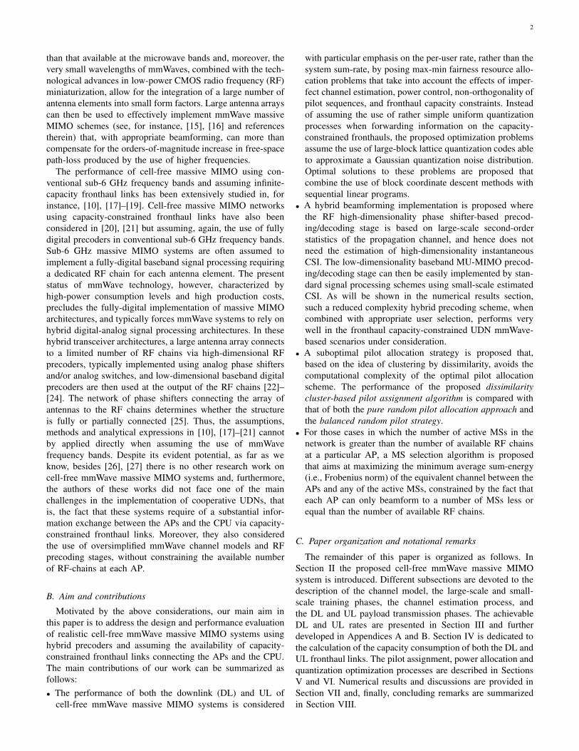
Large-scaleTraining

CoherenceInterval

CoherenceInterval

CoherenceInterval

τLc

τc τc τc

τc

τp τu τd

Uplink pilots Uplink payload data Downlink payload data

Fig. 1: Allocation of the samples in large-scale and short-scale

coherence intervals.

Notation: Vectors and matrices are denoted by lower-case

and upper-case boldface symbols. The q-dimensional identity

matrix is represented by Iq . The operator det(X) represents

the determinant of matrix X , tr(X) denotes its trace, ‖X‖F is

its Frobenius norm, whereas X−1, XT , X∗ and XH denote

its inverse, transpose, conjugate and conjugate transpose (also

known as Hermitian), respectively. With a slight abuse of

notation, the operator diag(x) is used to denote a diagonal

matrix with the entries of vector x on its main diagonal, and

the operator diag(X) is used to denote a vector containing

the entries in the main diagonal of matrix X . The expectation

operator is denoted by E·. Finally, CN (m,R) denotes a

circularly symmetric complex Gaussian vector distributions

with mean m and covariance R, N (0, σ2) denotes a real

valued zero-mean Gaussian random variable with standard de-

viation σ, and U [a, b] represents a random variable uniformly

distributed in the range [a, b].

II. SYSTEM MODEL

Let us consider a cell-free massive MIMO system where

a CPU coordinates the communication between M APs and

K single-antenna MSs randomly distributed in a large area.

Each of the APs communicates with the CPU via error-free

fronthaul links with DL and UL capacities CF d and CF u,

respectively. Baseband processing of the transmitted/received

signals is performed at the CPU, while the RF operations are

carried out at the APs. Each AP is equipped with an array of

N > K antennas and L ≤ N RF chains. A fully-connected

architecture is considered where each RF chain is connected

to the whole set of antenna elements using N analog phase

shifters. Without loss of essential generality, it is assumed in

this paper that the number of active RF chains at each of the

APs in the network is equal to LA = minK,L. That is, if

K ≤ L, all APs in the cell-free network provide service to

the whole set of MSs and if K > L, instead, each AP can

only provide service to L out of the K MSs in the network

and, thus, an algorithm must be devised to decide which are

the MSs to be beamformed by each of the APs.

The propagation channels linking the APs to the MSs

are typically characterized by small-scale parameters that are

(almost) static over a coherence time-frequency interval of

τc time-frequency samples (see [3, Chapter 2]), and large-

scale parameters (i.e., path loss propagation losses and co-

variance matrices) that can be safely assumed to be static

over a time-frequency interval τLc ≫ τc. As shown in the

following subsections, these channel characteristics can be

leveraged to simplify both the channel estimation and the

precoding/combining processes. In particular, DL and UL

transmissions between APs and MSs are organized in a half-

duplex TDD operation whereby each coherence interval is

split into three phases, namely, the UL training phase, the

DL payload data transmission phase and the UL payload data

transmission phase, and every large-scale coherence interval

τLc the system performs an estimation of the large-scale

parameters of the channel (see Fig. 1). In the UL training

phase, all MSs transmit UL training orthogonal pilots allowing

the APs to estimate the propagation channels to every MS in

the network1. Subsequently, these channel estimates are used

to detect the signals transmitted from the MSs in the UL

payload data transmission phase and to compute the precoding

filters governing the DL payload data transmission. Not shown

are guard intervals between UL and DL transmissions.

A. Channel Model

MmWave propagation is characterized by very high

distance-based propagation losses that lead to sparse scatter-

ing multipath propagation. Furthermore, the use of mmWave

transmitters and receivers with large tightly-packet antenna

arrays results in high antenna correlation levels. These char-

acteristics make most of the statistical channel models used

in conventional sub-6 GHz MIMO research work inaccurate

when dealing with mmWave scenarios. Thus, a modified

version of the discrete-time narrowband clustered channel

model proposed by Akdeniz et al. in [13] and further extended

by Samimi and Rappaport in [28] will be used in this paper

to capture the peculiarities of mmWave channels.

The link between the mth AP and the kth MS will be

considered to be in one out of three possible conditions:

outage, line-of-sight (LOS) or non-line-of-sight (NLOS) with

probabilities:

pout(dmk) = max(

0, 1− e−aoutdmk+bout)

, (1a)

pLOS(dmk) = (1− pout(dmk)) e−aLOSdmk , (1b)

pNLOS(dmk) = 1− pout(dmk)− pLOS(dmk), (1c)

respectively, where dmk is the distance (in meters) between

the AP and the MS, and, according to [13, Table I], 1/aout =30 m, bout = 5.2, and 1/aLOS = 67.1 m. Those links that are

in outage will be characterized with infinite propagation losses,

while for the links that are not in outage, the propagation

losses will be characterized using a standard linear model with

shadowing as

PL(dmk)[dB] = α+ 10β log10(dmk) + χmk, (2)

where α and β are the least square fits of floating intercept and

slope and depend on the carrier frequency and on whether the

link is in LOS or NLOS (see [13, Table I]), and χmk denotes

the large-scale shadow fading component, which is modelled

1Note that channel reciprocity can be exploited in TDD systems andtherefore only UL pilots need to be transmitted.

4

as a zero mean spatially correlated normal random variable

with standard deviation σχ (again, see [13, Table I] to obtain

the typical values of σχ for LOS and NLOS links) whose

spatial correlation model is described in [10, (54)-(55)].

The UL channel vector hmk ∈ CN×1 between MS k and

AP m will be modelled as the sum of the contributions of

Cmk scattering clusters, each contributing Pmk propagation

paths as

hmk =

Cmk∑

c=1

Pmk∑

p=1

αmk,cpa (θmk,cp, φmk,cp) , (3)

where αmk,cp is the complex small-scale fading gain on the

pth path of cluster c, and a (θmk,cp, φmk,cp) represents the AP

normalized array response vector at the azimuth and elevation

angles θmk,cp and φmk,cp, respectively. These angles, as stated

by Akdeniz et al. in [13, Section III.E] can be generated

as wrapped Gaussians around the cluster central angles with

standard deviation given by the root mean square (rms) angular

spreads for the cluster. The azimuth cluster central angles are

uniformly distributed in the range [−π, π] and the elevation

cluster central angles are set to the LOS elevation angle.

Moreover, the cluster rms angular spreads are exponentially

distributed with a mean equal to 1/λrms that depends on

the carrier frequency and on whether we are considering the

azimuth or elevation directions (see [13, Table I]). The number

of clusters is distributed as a random variable of the form

Cmk ∼ max Poisson(σC), 1 , (4)

where σC is set to the empirical mean of Cmk. The small-scale

fading gains are distributed as

αmk,cp ∼ CN(

0, γmk,c10−PL(dmk)/10

)

, (5)

where the cluster c is assumed to contribute with a fraction of

power given by

γmk,c =Nγ′

mk,c

Pmk

∑Cmk

j=1 γ′mk,j

, (6)

with

γ′mk,j = U rτ−1

mk,j 10Zmk,j/10, (7)

Umk,j ∼ U [0, 1], Zmk,j ∼ N (0, ζ2), and the constants rτ and

ζ2 being treated as model parameters (see [13, Table I]).

Although the small-scale fading gains αmk,cp are assumed

to be static throughout the coherence interval and then change

independently (i.e., block fading), the spatial covariance ma-

trices

Rmk =E

hmkhHmk

=10−PL(dmk)/10Cmk∑

c=1

γmk,c

×Pmk∑

p=1

a (θmk,cp, φmk,cp)aH (θmk,cp, φmk,cp) ,

(8)

are assumed to vary at a much smaller pace (i.e., τLc ≫ τc).

B. Large-scale training phase

1) RF precoder/combiner design: In order to exploit the

UL/DL channel reciprocity using the TDD frame structure

shown in Fig. 1, it is assumed in this paper that the N×LA RF

matrix WRFm , describing the effects of the active analog phase

shifters at the mth AP, is common to the DL (RF precoding

phase) and UL (RF combining phase). Furthermore, denoting

by Km = κm1, . . . , κmLA the set of LA MSs beamformed

by the mth AP, it is assumed that WRFm is a function of only

the spatial channel covariance matrices Rmkk∈Km, known

at the mth AP through spatial channel covariance estimation

for hybrid analog-digital MIMO precoding architectures (see

e.g. [29]–[32]).

Using eigen-decomposition, the covariance matrix of the

propagation channel linking MS k and AP m can be

expressed as Rmk = UmkΛmkUHmk, where Λmk =

diag ([λmk,1 . . . λmk,rmk]) contains the rmk non-null eigen-

values of Rmk, and Umk is the N × rmk matrix of the

corresponding eigenvectors. Hence, assuming the use of (con-

strained) statistical eigen beamforming [33], [34], the analog

RF precoder/combiner can be designed as

WRFm =

[

wRFmκm1

. . . wRFmκmLA

]

=[

e−j∠umκm1,max . . . e−j∠umκmLA

,max

]

,(9)

where umk,max is the dominant eigenvector of Rmk associated

to the maximum eigenvalue λmk,max, and the function ∠x re-

turns the phase angles, in radians, for each element of the com-

plex vector x. Note that using the RF precoding/combining

matrix, the equivalent channel vector between MS k and AP

m, including the RF precoding/decoding matrix, is defined as

gmk = WRFm

Thmk ∈ C

LA×1, (10)

whose dimension is much less than the number of antennas

of the massive MIMO array used at the mth AP, thus largely

simplifying the small-scale training phase.

2) Selection of MSs to beamform from each AP: As pre-

viously stated, in those highly probable cases in which the

number of active MSs in the network is greater than the

number of available RF chains at each AP (i.e., K > L), the

mth AP, with m ∈ 1, . . . ,M, can only beamform to a group

of L out of the K MSs in the network, which are indexed

by the set Km = κm1, . . . , κmL. As the RF beamforming

matrices at the APs are a function of only the large-scale

spatial channel covariance matrices and are common to both

the UL and the DL, the selection of the sets of MSs to

beamform from each AP must also be based only on the

available large-scale CSI. Inspired by the Frobenius norm-

based suboptimal user selection algorithm proposed by Shen

et al. in [35], a selection algorithm is proposed that aims

at maximizing the sum of the average energy (i.e., average

Frobenius norm) of the equivalent channels (including the

corresponding beamformer) between the M APs and the KMSs with the constraints that, first, the minimum average

energy of the equivalent channel between the M APs and any

of the active MSs must be maximized and, second, that each

AP can only beamform to L MSs. Note that this optimization

5

problem, which tends to provide some degree of (average)

max-min fairness among MSs, can be efficiently solved by

using an iterative reverse-delete algorithm (similar to that used

in graph theory to obtain a minimum spanning tree from

a given connected, edge-weighted graph). In particular, at

the beginning of the ith iteration of the algorithm the cell-

free network is represented by a very simple edge-weighted

directed graph with M source nodes and K sink nodes, where

the mth source node, representing the mth AP, is connected

to a group K(i)m of sink nodes, representing the active MSs

beamformed by the mth AP. The connection (edge) between

the mth source node and the lth sink node in K(i)m is weighted

by the average Frobenius norm of the equivalent channel

linking the mth AP and MS l ∈ K(i)m , that can be obtained as

ξml = E

∥

∥

∥wRF

ml

Thml

∥

∥

∥

2

F

= wRFml

TRmlw

RFml . (11)

The average sum energy of the equivalent channels between

the M APs and MS k at the beginning of the ith iteration is

E(i)k =

∑

m∈M(i)k

ξmk, (12)

where M(i)k is the set of APs beamforming to MS k at the

beginning of the ith iteration. During this iteration, the reverse-

delete algorithm removes the edge (i.e., the RF chain and

associated beamformer) that, first, goes out of one of those

APs still beamforming to more than L MSs and, second,

has the minimum weight maximizing the minimum average

sum energy after removal. The algorithm begins with a fully

connected graph and stops when all APs beamform to exactly

L MSs. Hence, note that M(K − L) iterations are needed to

select the sets Km for m ∈ 1, . . . ,M.

C. Small-scale training phase

Communication in any coherence interval of a TDD-based

massive MIMO system invariably starts with the MSs sending

the pilot sequences to allow the channel to be estimated at the

APs. Let τp denote the UL training phase duration (measured

in samples on a time-frequency grid) per coherence interval.

During the UL training phase, all K MSs simultaneously

transmit pilot sequences of τp samples to the APs and thus,

the LA× τp received UL signal matrix at the mth AP is given

by

Y pm =√

τpPp

K∑

k′=1

gmk′ϕTk′ +Npm, (13)

where Pp is the transmit power of each pilot symbol, ϕk

denotes the τp × 1 training sequence assigned to MS k,

with ‖ϕk‖2F = 1, and Npm is an LA × τp matrix of

i.i.d. additive noise samples with each entry distributed as2

CN (0, σ2u(N)). Ideally, training sequences should be chosen

to be mutually orthogonal, however, since in most practical

scenarios it holds that K > τp, a given training sequence

is assigned to more than one MS, thus resulting in the so-

called pilot contamination, a widely studied phenomenon in

the context of collocated massive MIMO systems [36].

D. Channel estimation

Channel estimation is known to play a central role in the

performance of massive MIMO schemes [37] and also in the

specific context of cell-free architectures [10]. The minimum

mean square error (MMSE) estimation filter for the channel

between the kth active MS and the mth AP can be calculated

as

Dmk = argminD

E

∥

∥gmk −DY pmϕ∗k

∥

∥

2

=√

τpPpRRFmkQ

−1mk,

(14)

where

RRFmk = E

gmkgHmk

= WRFm

TRmkW

RFm

∗, (15)

and

Qmk = τpPp

K∑

k′=1

RRFmk′

∣

∣ϕTk′ϕ∗

k

∣

∣

2+ σ2

u(N)ILA. (16)

Hence, the corresponding estimated channel vector can be

expressed as

gmk = DmkY pmϕ∗k =

√

τpPpRRFmkQ

−1mkY pmϕ∗

k. (17)

The MMSE channel vector estimates can be shown to be

distributed as gmk ∼ CN(

0, RRF

mk

)

, where

RRF

mk , τpPpRRFmkQ

−1mkR

RFmk

H. (18)

Furthermore, the channel vector gmk can be decomposed

as gmk = gmk + gmk, where gmk is the MMSE channel

estimation error, which is statistically independent of both gmk

and gmk.

E. Downlink payload data transmission

Let us define sd = [sd1 . . . sdK ]T

as the K × 1 vector

of symbols jointly (cooperatively) transmitted from the APs

to the MSs, such that E

sdsHd

= IK . Let us also define

xm = Pm (sd) as the N×1 vector of signals transmitted from

the mth AP, where Pm (sd) is used to denote the mathematical

operations (linear and/or non-linear) used to obtain xm from

2Note that in the UL of a fully-connected hybrid beamforming architectureeach reception chain is composed of N antenna elements, each connectedto a low-noise amplifier (LNA) characterized by a power gain GLNA anda noise temperature TLNA . Each of the N LNAs feeds an analog passivephase shifter characterized by an insertion loss LPS. The outputs of the Nphase shifters are introduced to a power combiner whose insertion lossesare typically proportional to the number of inputs, that is, LPC = NLPCin

.Finally, the output of the power combiner is introduced to an RF chaincharacterized by a power gain GRF and a noise temperature TRF. Thus, theequivalent noise temperature of each receive chain can be obtained as Tu =

N(

T0 + TLNA +T0(LPSLPCin

−1)

GLNA+

TRFLPSLPCinGLNA

)

.

6

sd. Note that this vector must comply with a power constraint

E

‖xm‖2F

≤ Pm, where Pm is the maximum average

transmit power available at AP m. Using this notation, the

signal received by MS k can be expressed as

ydk =

M∑

m=1

hTmkxm + ndk, (19)

where ndk ∼ CN (0, σ2d) is the Gaussian noise sample at MS

k. The vector yd = [yd1 . . . ydK ]T containing the signals

received by the K scheduled MSs in the network can then

be expressed as

yd =

M∑

m=1

HTmxm + nd, (20)

where Hm = [hm1 . . . hmK ] and nd = [nd1 . . . ndK ]T .

The mathematical operations that symbol vector sd un-

dergoes before being transmitted, generically represented as

xm = Pm(sd), for all m ∈ 1, . . . ,M, include, first, a

baseband precoding task at the CPU, second, a compressing

process of all or part of the data that must be sent from

the CPU to the APs through the fronthaul links and, third,

an RF precoding task at each of the APs. Let us denote by

Qdm(x) and Qd−1m (x) the quantization and unquantization

mathematical operations performed by the compress-after-

precoding (CAP)-based CPU-AP functional split on a vector

of signal samples x to be transmitted by the mth AP. Due to

the distortion introduced by the quantization/unquantization

processes, we have that [38], [39]

Qdm(x) , Qd−1m (Qdm(x)) = x+ qdm, (21)

where qdm is the quantization noise vector, which is assumed

to be statistically distributed as qdm ∼ CN(

0, σ2qdmI

)

. As

shown by Zamir et al. in [38], this assumption is supported by

the fact that large-block lattice quantization codes are able to

approximate a Gaussian quantization noise distribution. Thus,

the mathematical operations describing the CPU-AP functional

split considered in this paper can be summarized as

xm = Pm(sd) = WRFm Qdm

(

WBBdmΥ

1/2sd

)

= WRFm

(

WBBdmΥ

1/2sd + qdm

)

,(22)

where WBBd =

[

WBBd 1

T. . . WBB

dM

T]T

∈ CMLA×K ,

with WBBdm =

[

wBBdm1 . . . wBB

dmK

]

∈ CLA×K denoting the

baseband precoding matrix affecting the signal transmitted by

the mth AP, and Υ = diag ([υ1 . . . υK ]) is a K×K diagonal

matrix containing the power control coefficients in its main

diagonal, which are chosen to satisfy the following necessary

power constraint at the mth AP

E

‖xm‖2F

=K∑

k=1

υkθBB/RFmk + σ2

q dm

∥

∥

∥WRF

m

∥

∥

∥

2

F

=K∑

k=1

υkθBB/RFmk + σ2

q dmLAN ≤ Pm,

(23)

where we have used the definition

θBB/RFmk = E

∥

∥

∥WRF

m wBBdmk

∥

∥

∥

2

F

. (24)

Using the proposed hybrid CAP approach, the signal re-

ceived by the K MSs can be rewritten as

yd =M∑

m=1

HTmWRF

m WBBdmΥ

1/2sd

+M∑

m=1

HTmWRF

m qdm + nd

= GTWBBd Υ

1/2sd + ηd,

(25)

where G = [GT1 . . . GT

M ]T , with Gm = WRFm

THm,

representing the equivalent MIMO channel matrix between the

K MSs and the M APs, including the RF precoding/decoding

matrices, and

ηd = GTqd + nd, (26)

with qd = [qdT1 . . . qd

TM ]T , includes the thermal noise as well

as the quantization noise samples received from all the APs in

the network. Now, using the classical ZF MU-MIMO baseband

precoder to harness the spatial multiplexing, we have that

WBBd = G

∗(

GTG

∗)−1

(27)

or, equivalently,

WBBdm = G

∗

m

(

GTG

∗)−1

∀m, (28)

where we have assumed that G = G+ G and Gm = Gm +Gm. Consequently, the signal received by the kth MS can be

expressed as

ydk =gTk G

∗(

GTG

∗)−1

Υ1/2sd + ηdk

=(

gTk + gT

k

)

G∗(

GTG

∗)−1

Υ1/2sd + ηdk

=√υksdk + gT

k G∗(

GTG

∗)−1

Υ1/2sd + ηdk

(29)

where ηdk = gTk qd + ndk. The first term denotes the useful

received signal, the second term contains the interference

terms due to the use of imperfect CSI (pilot contamination),

and the third term encompass both the quantification and

thermal noise samples.

F. Uplink payload data transmission

In the UL, the vector of received signals at the output of

the LA RF chains (including the RF phase shifters) of the mth

AP is given by

rum =√

Pu

K∑

k′=1

gmk′

√ωk′suk′ + num

=√

PuGmΩ1/2su + num,

(30)

where Pu is the maximum average UL transmit power avail-

able at any of the active MSs, su = [su1 . . . suK ]T denotes

the vector of symbols transmitted by the K active MS,

7

Ω = diag([ω1 . . . ωK ]), with 0 ≤ ωk ≤ 1, is a matrix

containing the power control coefficients used at the MSs,

and num ∼ CN (0, σ2u(N)ILA

) is the vector of additive

thermal noise samples at the output of the LA RF chains of

the mth AP. The received vector of signals at each of the

APs in the network is quantized and forwarded to the CPU

via the UL fronthaul links, where they are unquantized and

jointly processed using a set of baseband combining vectors.

Using a similar approach to that employed to model the DL

transmission, the received vector of (unquantized) samples

from the mth AP can be expressed as

zum = Qum (rum) = rum + qum, (31)

where qum is the quantization noise vector, which is assumed

to be statistically distributed as qum ∼ CN(

0, σ2qum

ILA

)

.

Now, assuming the use of ZF MIMO detection, the CPU uses

the detection matrix

WBBu =

(

GHG)−1

GH

= WBBd

T(32)

or, equivalently

WBBum =

(

GHG)−1

GH

m = WBBdm

T, ∀m, (33)

to jointly process the vector zu =[

zuT1 . . . zu

TM

]Tand obtain

the vector of detected samples

yu =WBBu zu =

√

PuWBBu GΩ

1/2su + ηu

=√

PuΩ1/2su +

√

PuWBBu GΩ

1/2su + ηu,(34)

where ηu = WBBu (qu + nu). Again, the first term denotes

the useful received signal, the second term contains the in-

terference terms due to the use of imperfect CSI, and the

third term includes both the quantification and thermal noise

samples. The detected sample corresponding to the symbol

transmitted by the kth MS can then be obtained as

yuk =√

Puω1/2k suk+

√

Pu

[

WBBu GΩ

1/2su

]

k+ηuk, (35)

where [x]k denotes the kth entry of vector x.

III. ACHIEVABLE RATES

Analysis techniques similar to those applied, for instance,

in [3], [10], [17], [40]–[42], are used in this section to derive

DL and UL achievable rates. In particular, the sum of the

second and third terms on the right hand side (RHS) of (29),

for the DL case, and (35), for the UL case, are treated as

effective noise. The additive terms constituting the effective

noise are, in both DL and UL cases, mutually uncorrelated,

and uncorrelated with sdk and suk, respectively. Therefore,

both the desired signal and the so-called effective noise are

uncorrelated. Now, recalling the fact that uncorrelated Gaus-

sian noise represents the worst case, from a capacity point

of view, and that the complex-valued fast fading random

variables characterizing the propagation channels between

different pairs of AP-MS connections are independent, the

DL and UL achievable rates (measured in bits per second per

Hertz) for MS k can be obtained as stated in the following

theorems:

Theorem 1 (Downlink achievable rate). An achievable rate

of MS k using the analog precoders WRFm , for all m ∈

1, . . . ,M, and the ZF baseband precoder WBBd =

G∗(

GTG

∗)−1

is Rdk = log2 (1 + SINRdk), with

SINRdk =υk

∑Kk′=1 υk′kk′ + σ2

ηdk

, (36)

where

σ2ηdk

=

M∑

m=1

σ2q dm

tr(

RRFmk

)

+ σ2d, (37)

and

kk′ =[

diag(

E

WBBd

Hg∗kg

TkW

BBd

)]

k′

. (38)

Proof. See Appendix A.

Theorem 2 (Uplink achievable rate). An achievable UL rate

for the kth MS in the Cell-Free Massive MIMO system with

limited capacity fronthaul links and using ZF MIMO detection,

for any M , N and K , is given by Ruk = log2 (1 + SINRuk),with

SINRuk =Puωk

Pu

∑Kk′=1 ωk′δkk′ + σ2

ηuk

, (39)

where

δkk′ =[

diag(

E

GHwBB

uk

HwBB

uk G)]

k′

(40)

with wBBuk denoting the kth row of WBB

u , or, equivalently,

δkk′ =[

diag(

E

WBBu gk′ g

Hk′W

BBu

H)]

k, (41)

and

σ2ηuk

=

M∑

m=1

(

σ2q um

+ σ2u(N)

)

νumk, (42)

with

νumk =[

diag(

E

WBBumWBB

um

H)]

k. (43)

Proof. See Appendix B.

IV. FRONTHAUL CAPACITY CONSUMPTION

The DL quantization process performed at the mth AP can

be expressed as

Qdm

(

WBBdmΥ

1/2sd

)

= WBBdmΥ

1/2sd + qdm. (44)

From standard random coding arguments [43], vector sdcan be safely assumed to be distributed as sd ∼ CN (0, IK)

and thus, the quantized vector Qdm

(

WBBdmΥ

1/2sd

)

is distributed as Qdm

(

WBBdmΥ

1/2sd

)

∼CN

(

0,WBBdmΥWBB

dm

H+ σ2

qdmILA

)

. Furthermore, as

the differential entropy of a vector x ∼ CN (ω,Θ) is given

by H(x) = log det(πeΘ) [43], the required average rate

to transfer the quantized vector Qdm

(

WBBdmΥ

1/2sd

)

on

8

the corresponding DL fronthaul link can be obtained as (in

bps/Hz)

Cdm = E

I(

Qdm

(

WBBdmΥ

1/2sd

)

;WBBdmΥ

1/2sd

)

= E

H(

Qdm

(

WBBdmΥ

1/2sd

))

− E

H(

Qdm

(

WBBdmΥ

1/2sd

)

∣

∣WBBdmΥ

1/2sd

)

= E

log2 det

(

1

σ2qdm

WBBdmΥWBB

dm

H+ ILA

)

,

(45)

where I(x;x) is used to denote the mutual information

between vectors x and x, and H(x|x) is the differential

entropy of x conditioned on x. Since the determinant is a log-

concave function on the set of positive semidefinite matrices,

it follows from Jensen’s inequality that

Cdm ≤ log2 det

(

1

σ2qdm

E

WBBdmΥWBB

dm

H

+ ILA

)

= log2 det

(

1

σ2qdm

K∑

k=1

υkRBBmk + ILA

)

,

(46)

where RBBmk = E

wBBmkw

BBmk

H

.

Analogously, the UL quantization process performed at the

mth AP is given by Qum (rum) = rum + qum. Thus, using

arguments similar to those used in the DL case, the required

average rate to transfer the quantized vector Qum (rum) on

the corresponding UL fronthaul link can be upper bounded as

(in bps/Hz)

Cum = E

I(

Qum (rum) ; rum

)

= E

H(

Qum (rum))

− E

H(

Qum (rum)∣

∣rum

)

≤ log2 det

(

Pu

σ2q um

K∑

k=1

ωkRRFmk +

(

σ2u(N)

σ2q um

+ 1

)

ILA

)

.

(47)

V. PILOT ASSIGNMENT

To warrant an appropriate system performance, the radio

resource management (RRM) unit must efficiently manage

both the pilot assignment and the UL and DL power control.

As the pilots are not power controlled, pilot assignment and

power control can be conducted independently. Since the

length of the pilot sequences is limited to τp, there only exist

τp orthogonal pilot sequences. In a network with K ≤ τpMSs, an optimal pilot assignment strategy simply allocates Korthogonal pilots to the K MSs. The real pilot assignment

problem arises when K > τp. In this case, fully orthogonal

pilot assignment is no longer possible and hence, other pilot

assignment strategies must be devised.

On the one hand, designing an optimal pilot assignment

strategy aiming at maximizing the minimum rate allocated

to the active MSs in the network is a very difficult com-

binatorial problem, computationally unmanageable in most

network setups of practical interest [10]. On the other hand,

using straightforward strategies such as, for instance, the pure

random pilot assignment (RPA) scheme [44], where each

MS is randomly assigned one pilot sequence out of the set

of τp orthogonal pilot sequences, or the balanced random

pilot assignment (BRPA) scheme, where each MS is allocated

a pilot sequence that is sequentially and cyclically selected

from the ordered set of available orthogonal pilots, provides

poor performance results. In order to avoid the computational

complexity of the optimal strategies while improving the

performance of the baseline RPA or BRPA approaches, a

suboptimal solution is proposed in this paper that is based

on the idea of clustering by dissimilarity. This suboptimal

approach, that will be termed as the dissimilarity cluster-

based pilot assignment (DCPA) strategy, is motivated by the

following key observation:

Key observation: In those scenarios where K > τp,

cell-free communication is severely impaired whenever MSs

showing very similar large-scale propagation patterns to the

set of APs (that is, MSs typically located nearby) are allocated

the same pilot sequence. In this case, the inter-MS interference

leads to very poor channel estimates at all APs and, eventually,

to low signal-to-interference-plus-noise ratios (SINRs).

The clustering algorithm proposed in this work basically

ensures that pilot sequences are only reused by MSs showing

dissimilar large-scale propagation patterns to the APs (that

is, MSs typically located sufficiently apart). Two key aspects

regarding the clustering operation are thus, on the one hand,

to decide which should be the large-scale propagation pattern

that ought to be used to represent a given MS and, on the other

hand, to decide what metric should be used to measure similar-

ity among the large-scale propagation patterns characterizing

different MSs. To this end, and resting upon the premise that

the CPU has perfect knowledge of the large-scale gains, let

ξk = [ξ1k . . . ξMk]T

denote the M × 1 vector containing the

average Frobenius norms of the equivalent channels linking

the kth MS to all M APs in the cell-free network. Vector ξkcan be considered as an effective fingerprint characterizing the

location of MS k. Now, although no single definition of a sim-

ilarity measure exists, the so-called cosine similarity measure

is one of the most commonly used similarity metrics when

dealing with real-valued vectors. Hence, as the fingerprint

vectors characterizing the different MSs are non-negative real-

valued, the cosine similarity measure between two fingerprint

vectors ξk and ξk′ , defined as

fD (ξk, ξk′ ) =ξTk ξk′

‖ξk‖2‖ξk′‖2, (48)

will be used as a proper similarity metric in our work. The

resulting similarity values range from 0, meaning orthogonal-

ity (perfect dissimilarity), to 1, meaning exact match (perfect

similarity).

The proposed DCPA algorithm proceeds as follows. In a first

step, it calculates the fingerprint of an imaginary MS centroid,

defined as

ξC =1

K

K∑

k=1

ξk. (49)

9

Then, it moves onward to the calculation of the cosine similar-

ity measures among the fingerprint vectors characterizing the

K MSs in the network and the fingerprint of the centroid, that

is, the algorithm proceeds to the calculation of fD (ξk, ξC),for all k ∈ 1, . . . ,K. The MSs are then sorted in descending

order of similarity with the centroid, that is, the algorithm ob-

tains the ordered set of subindices O = o1, o2, . . . , oK, such

that fD(

ξo1 , ξC)

≤ fD(

ξo2 , ξC)

≤ · · · ≤ fD(

ξoK , ξC)

.

Once the MSs have been sorted, the algorithm constructs τpclusters of MSs, namely K1, . . . ,Kτp , with

Kt =O (t : τp : K)

=

ot, ot+τp , ot+2τp , . . .

, ∀t ∈ 1, . . . , τp,(50)

and all MSs in cluster Kt, which are located far from each

other, are allocated the same pilot code ϕt. Note that the appli-

cation of this algorithm ensures that, as far as it is possible, two

MSs having similar large-scale propagation fingerprints are

allocated different pilot codes and, thus, they do not interfere to

each other during the UL channel estimation process. In other

words, it aims at minimizing the residual interuser interference

terms in both (29) and (35).

VI. MAX-MIN POWER ALLOCATION AND OPTIMAL

QUANTIZATION

A. Downlink power control and quantization

In line with previous research works on cell-free architec-

tures [9], [10], [17], [20], our aim in this subsection is to find

the power control coefficients υk, for all k ∈ 1, . . . ,K,

and the quantization noise variances σ2q dm

, for all m ∈1, . . . ,M, that maximize the minimum of the achievable

DL rates of all MSs while satisfying the average transmit

power and DL fronthaul capacity constraints at each AP.

Mathematically, this optimization problem can be formulated

as

maxΥ0σqd

0

mink∈1,...,K

υk∑K

k′=1 υk′kk′ + σ2ηdk

s.t.

K∑

k=1

υkθBB/RFmk ≤ Pm − σ2

q dmLAN, ∀m,

log2 det

(

K∑

k=1

υkσ2q dm

RBBmk + ILA

)

≤ CF d, ∀m,

(51)

where we have used the definition σqd = [σqd1 . . . σqdM ]T .

Optimization problem (51) is characterized by continuous

objective and constraint functions of interdependent block

variables, namely, Υ and σqd. A widely used approach

for solving optimization problems of this class is the so-

called block coordinate descend (BCD) method. This is an

iterative optimization approach that, at each iteration and in a

cyclic order, optimizes one of the blocks while the remaining

variables are held fixed [45], [46]. Convergence of the BCD

method is ensured whenever each of the subproblems to be

optimized in each iteration can be exactly solved to its unique

optimal solution.

The first important fact to note is that, given a power

allocation matrix Υ(i−1) obtained at the (i − 1)th iteration,

and as the achievable user rates monotonically increase with

the capacity of the fronthaul links between the APs and

the CPU, the optimal solution for the acceptable fronthaul

quantization noise in the ith iteration is achieved when the

fronthaul capacity constraints are satisfied with equality, that

is, when

det

(

K∑

k=1

υ(i−1)k

σ2q(i)

dm

RBBmk + ILA

)

= 2CF d , ∀m. (52)

Note that σ2q(i)

dmcannot be expressed in a closed-form algebraic

expression as it only admits a solution in the form of a

transcendental function

σ2q(i)

dm= Fd

(

Υ(i−1),

RBBmk

K

k=1, CF d

)

(53)

that can be numerically solved by applying mathematical

software tools to (52).

Once the optimal block of variables σq(i)d have been ob-

tained, the optimization problem in (51) can be rewritten in

terms of the power allocation matrix Υ(i) as

maxΥ(i)0

mink∈1,...,K

υ(i)k

K∑

k′=1

υ(i)k′ γkk′ +

M∑

m=1

σ2q

(i)

dmtr

(

RRFmk

)

+ σ2d

s.t.

K∑

k=1

υ(i)k θ

BB/RFmk ≤ Pm −NLAσ

2q(i)

dm, ∀m.

(54)

Note that this is a convergent quasi-linear optimization prob-

lem that can be solved using conventional standard convex

optimization methods [10], [17].

B. Uplink power control and quantization

In this subsection we aim at finding the power control

coefficients ωk, for all k ∈ 1, . . . ,K, and quantization

noise variances σ2qum

, for all m ∈ 1, . . . ,M, that maximize

the minimum of the achievable ulink rates of all MSs while

satisfying the power control coefficient constraints at each MS

and the UL fronthaul capacity constraints at each AP. This

optimization problem can be formulated as

maxω0

σqu0

mink∈1,...,K

Puωk

Pu

∑Kk′=1 ωk′δkk′ + σ2

ηuk

s.t. 0 ≤ ωk ≤ 1, ∀ k,

det

(

Pu

σ2q um

K∑

k=1

ωkRRFmk + ϑmILA

)

≤ 2CF u , ∀m,

(55)

where σqu = [σqu1 . . . σquM ]T , and we have used the

definition ϑm = 1 + σ2u(N)/σ2

q um. As for the DL case,

problem (55) admits the use of the BCD method where, in

each iteration, the nonconvex transcendental function σ2q um

=

Fu

(

Ω,

RRFmk

K

k=1, Pu, CF u

)

is approximated by a con-

stant calculated using the power allocation vector obtained

in the previous iteration of the algorithm. That is, in the ith

10

TABLE I: Summary of default simulation parameters

Parameters Value

Carrier frequency: f0 28 GHz

Bandwidth: B 20 MHz

Side of the square coverage area: D 200 m

AP antenna height: hAP 15 m

MS antenna height: hMS 1.65 m

Noise figure at the MS: NFMS 9 dB

Noise figure of the LNA at the AP: NFLNA 1.6 dB

Gain of the LNA at the AP: GLNA 22 dB

Attenuation of the phase splitters at the AP: LPS 3 dB

Attenuation of the power combiner at the AP: LPCin 3 dB

Noise figure of the RF chain at the AP: NFRF 7 dB

Available average power at the AP: Pm 200 mW

Available average power at the MS: Pu = Pp 100 mW

Coherence interval length: τc 200 samples

Training phase length: τp 15 samples

iteration of the UL optimal power allocation approach, the

algorithm solves the optimization problem

maxΩ(i)0

mink∈1,...,K

Puω(i)k

Pu

∑Kk′=1 ω

(i)k′ δkk′ + σ

2(i)ηuk

,

s.t. 0 ≤ ωk ≤ 1, ∀ k,(56)

where σ2q(i)

um= Fu

(

Ω(i−1),

RRFmk

K

k=1, Pu, CF u

)

. Note

that, again, this is a convergent quasi-linear optimization prob-

lem that can be solved using conventional convex optimization

methods [10], [17].

VII. NUMERICAL RESULTS

In this section, simulation results are obtained in order to

quantitatively study the performance of the proposed cell-free

mmWave massive MIMO network with constrained-capacity

fronthaul links. In particular, we demonstrate the impact of us-

ing different pilot allocation strategies, the effects of modifying

the capacity of the fronthaul links and the RF infrastructure

at the APs, and the repercussion of changing the density of

APs per area unit. For simplicity of exposition, and without

loss of essential generality, a cell-free scenario is considered

where the M APs and K MSs are uniformly distributed at

random within a square coverage area of size D × D m2.

As described in subsection II-A, a modified version of the

discrete-time narrowband clustered channel model proposed

by Akdeniz et al. in [13] is used in the performance evaluation.

The parameters necessary to implement this channel model

can be found in [13, Table I]. Furthermore, similar to what

was done by Ngo et al. in [10], a shadow fading spatial

correlation model with two components is also considered

(see [10, eqs. (54) and (55)]) where the decorrelation distance

is set to ddecorr = 50 m and the parameter δ is set to 0.5.

Default parameters used to set-up the simulation scenarios

under evaluation in the following subsections are summarized

in Table I.

A. Impact of the pilot allocation process

Our aim in this subsection is to benchmark the performance

of the proposed large-scale CSI-aware DCPA strategy against

0 10 20 30 40 50Number of users (K)

4

6

8

10

12

14

16

18

Average

max

-min

userrate

(bit/s/H

z)

Downlink

DCPABRPARPA

0 10 20 30 40 50Number of users (K)

4

6

8

10

12

14

16

18

Average

max

-min

userrate

(bit/s/H

z)

Uplink

DCPABRPARPA

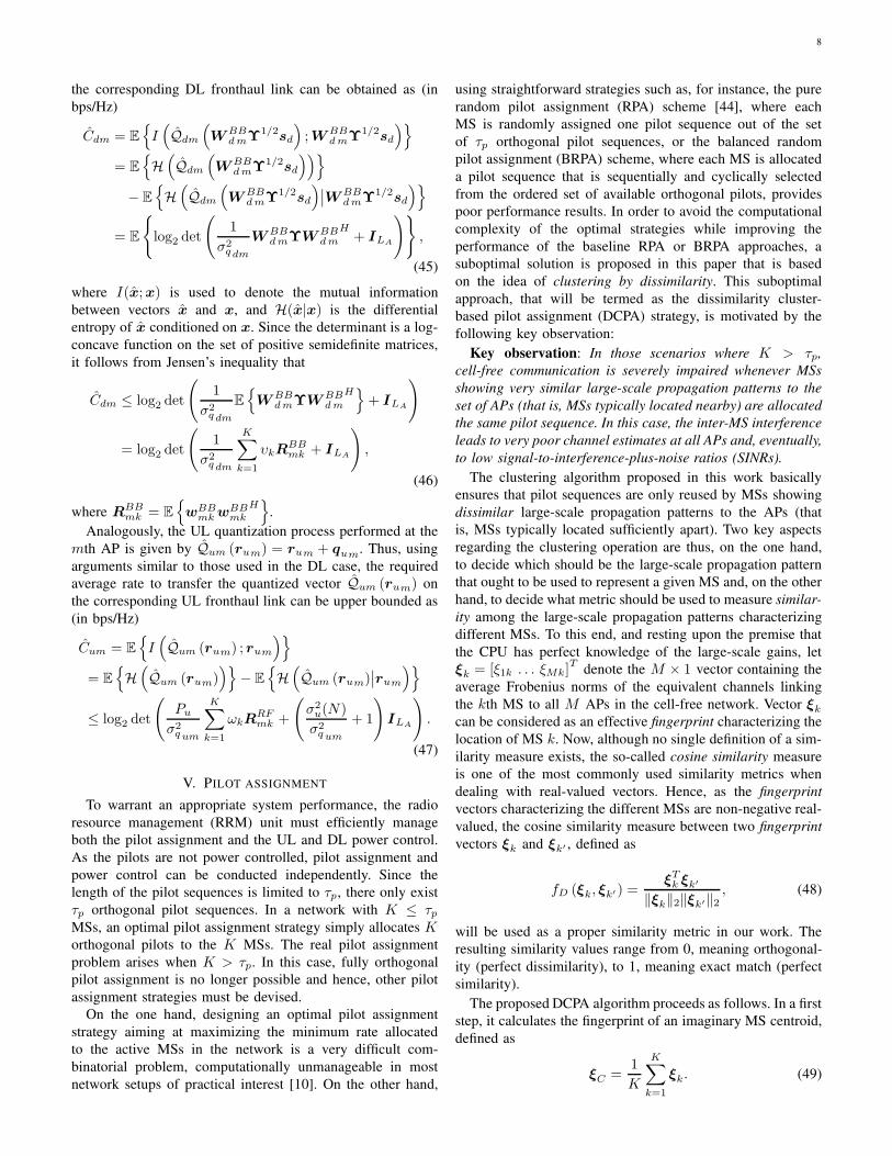
Fig. 2: Average max-min rate per user versus the number of activeMSs for different pilot allocation strategies (N = 64 antennas, L = 8

RF chains, CF d = CF u = 64 bit/s/Hz).

both the pure RPA and the BRPA schemes. Accordingly, the

average max-min rate per user versus the number of active

MSs is presented in Fig. 2 for each of these pilot allocation

strategies and for both the DL and the UL. All results

have been obtained assuming the default system parameters

described in Table I, the use of L = 8 RF chains fully

connected to uniform linear antenna arrays with N = 64antenna elements, and fronthaul links with a capacity of

CF d = CF u = 64 bit/s/Hz. The first important result to

note from Fig. 2 is that the pure RPA scheme is clearly

outperformed by both the BRPA and the DCPA strategies

irrespective of the of active MSs in the network. In fact,

the RPA scheme cannot guarantee neither the absence of

pilot reuse, even for those cases in which K ≤ τp (in this

setup, τp = 15 time/frequency samples), nor the possibility

of having pilots that are allocated to a high number of MSs

and/or to MSs exhibiting very similar large-scale propagation

patterns to the APs. Therefore, the higher the number of active

MSs, the higher the probability of having one or more users

suffering from high levels of pilot contamination, with the

consequent reduction of the achievable max-min user rate.

If we turn our attention to results provided by the BRPA

and DCPA strategies, two disjoint operation regions can be

distinguished. In the first one, comprising the scenarios in

which K ≤ τp, both approaches allocate orthogonal pilots to

the users (absence of pilot contamination) and thus naturally

provide the same performance. In the second one, however,

comprising the scenarios in which K > τp, pilots have to

be reused and, as a consequence, pilot contamination appears

(note the rather abrupt performance drop when going from

K ≤ τp to K > τp). In these scenarios, based on a smart

exploitation of the available large-scale CSI, the proposed

DCPA approach reduces the amount of pilot contamination

experienced by the worst users in the network and it clearly

improves the achievable max-min user rates provided by the

11

0 10 20 30 40 50Number of users (K)

4

6

8

10

12

14

16

18

Average

max

-min

userrate

(bit/s/H

z)

Downlink

CF d = 256 bps/HzCF d = 64 bps/HzCF d = 32 bps/HzCF d = 16 bps/Hz

0 10 20 30 40 50Number of users (K)

4

6

8

10

12

14

16

18

Average

max

-min

userrate

(bit/s/H

z)

Uplink

CF u = 256 bps/HzCF u = 64 bps/HzCF u = 32 bps/HzCF u = 16 bps/Hz

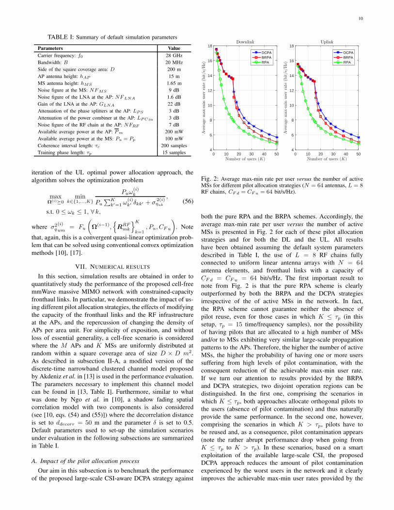
Fig. 3: Average max-min rate per user versus the number of activeMSs for different values of the fronthaul capacities (N = 64

antennas, L = 8 RF chains, DCPA).

channel-unaware BRPA scheme.

Another result that is worth emphasizing, since it will

repeatedly appear in the following subsections, is that, al-

though in scenarios with high-capacity fronthaul links the

achievable max-min DL user rate is higher than that provided

in the UL, as the number of active users in the network

increases, the performance obtained in both the DL and the

UL tend to become increasingly similar. This behavior can

be easily deduced from the analysis of the SINR expressions

in (36) and (39). As the number of active MSs in the cell-

free network increases, provided that it is greater than τp, the

term in the denominator corresponding to the residual interuser

interference due to pilot contamination becomes increasingly

dominant in comparison to the quantification and thermal

noise terms, eventually reaching the point where they can be

considered virtually negligible. Under these conditions, and

since the pre-coding filters used on both links are identical, the

DL and the UL experience similar SINR values and, therefore,

tend to provide the same achievable max-min rate per user,

except for small differences that can be attributed to, on the

one and, the dissimilar amount of quantified information that

has to be conveyed through the corresponding fronthaul links

and, on the other hand, disparities among the thermal noise

powers experienced at both the APs and the MSs.

B. Modifying the capacity of the fronthaul links and the RF

infrastructure at the APs

The max-min achievable rate per user is plotted in Fig. 3

against the number of active MSs in the network, assuming

the use of fronthaul links with different constraining capacities

equal to 16, 32, 64 and 256 bit/s/Hz (for the network setups

under consideration, using fronthaul links with a capacity of

256 bit/s/Hz is virtually equivalent to using infinite-capacity

fronthauls). As expected, results show that increasing the

fronthaul capacity is always beneficial if the main aim is to

0 10 20 30 40 50Number of users (K)

4

6

8

10

12

14

16

18

Average

max

-min

userrate

(bit/s/H

z)

Downlink

N = 128N = 64N = 32N = 16N = 8

0 10 20 30 40 50Number of users (K)

4

6

8

10

12

14

16

18

Average

max

-min

userrate

(bit/s/H

z)

Uplink

N = 128N = 64N = 32N = 16N = 8

Fig. 4: Average max-min rate per user versus the number of activeMSs for different values of the number of antennas at the APs (L = 8

RF chains, CF d = CF u = 64 bit/s/Hz, DCPA).

increase the achievable max-min user rate. Nevertheless, it is

worth stressing that, keeping all the other parameters constant,

the marginal increment of performance produced by each new

increment of the fronthaul capacity suffers from the law of

diminishing returns, especially for network setups with a high

number of active MSs. That is, although the performance

increase produced by doubling the fronthaul capacity from 16

bit/s/Hz to 32 bit/s/Hz, or even from 32 bit/s/Hz to 64 bit/s/Hz,

can be justifiable, increasing the fronthaul capacity beyond 64

bit/s/Hz does not seem to be reasonable from the point of view

of increasing the achievable performance of the system under

the considered network setups. As observed in the previous

subsection, in cell-free mmWave massive MIMO networks

using high-capacity fronthaul links, the achievable max-min

DL user rate is always slightly higher than that achieved in

the UL irrespective of the number of active MSs. In scenarios

with low-capacity fronthaul links and a large number of active

MSs, however, the quantization noise experienced in the DL

is higher than its UL counterpart and thus, the achievable per-

user rate in the UL is slightly higher that than supplied in the

DL.

To understand how the RF infrastructure used at the APs

influences the performance of the proposed cell-free mmWave

massive MIMO system under constrained-capacity fronthaul

links, Figs. 4 and 5 show the achievable max-min user rate

against the number of active MSs assuming the use of uniform

linear antenna arrays with different number of elements and

fully-connected analog RF precoders with different number of

RF chains, respectively. In particular, results presented in Fig.

4 have been obtained assuming the use of an analog precoder

with L = 8 RF chains fully-connected to a linear uniform

antenna array with N = 8, 16, 32, 64 or 128 antenna elements,

whereas results presented in Fig. 5 have been obtained assum-

ing the use of L = 2, 4, 8 or 16 RF chains fully-connected to

a linear uniform antenna array with N = 64 antenna elements.

12

0 10 20 30 40 50Number of users (K)

4

6

8

10

12

14

16

18

Average

max

-min

userrate

(bit/s/H

z)

Downlink

L = 2L = 4L = 8L = 16

0 10 20 30 40 50Number of users (K)

4

6

8

10

12

14

16

18

Average

max

-min

userrate

(bit/s/H

z)

Uplink

L = 2L = 4L = 8L = 16

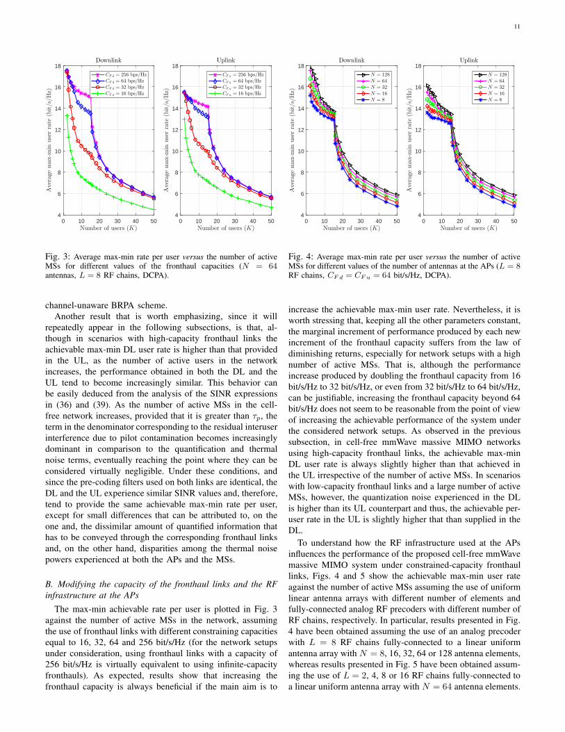
Fig. 5: Average max-min rate per user versus the number of activeMSs for different values of the number of RF chains at the APs(N = 64 antennas, CF d = CF u = 64 bit/s/Hz, DCPA).

The first conclusion we may draw when looking at the results

presented in Fig. 4 is that, irrespective of the number of active

MSs in the cell-free network, increasing the number of antenna

elements at the APs in scenarios with high capacity fronthaul

links (CF d = CF u = 64 bit/s/Hz), although moderate and

subject to the law of diminishing returns, always produces an

increase in the achievable max-min user rate. As shown in

Fig. 5, in contrast, the impact produced by an increase in the

number of RF chains at the APs depends on the number of

active MSs in the network. In particular, when the number

of active users is high, the interuser interference term due to

pilot contamination (imperfect CSI) dominates the factors in

the denominator of the SINR (i.e., makes the quantization and

thermal noises negligible) and thus, increasing the number of

RF chains is always beneficial when trying to increase the

achievable max-min user rate. When the number of active

users in the network is low, however, the quantization noise,

which is an increasing function of L, is not negligible anymore

when compared to the interuser interference term (recall that

this term is null when the number of active MSs is less than

or equal to τp) and thus, increasing the number of RF chains

at the APs can be clearly disadvantageous.

Results presented in Figs. 3, 4 and 5 were obtained assuming

high-capacity fronthaul links with CF d = CF u = 64 bit/s/Hz.

However, the amount of quantized data that has to be conveyed

from (to) the CPU to (from) the APs in the DL (UL) depends

on the number of antennas and RF chains at the APs (see

Section IV). Thus, in order to deepen in the study of the impact

the RF infrastructure may have on the achievable performance

of the proposed cell-free mmWave massive MIMO system

under constrained-capacity fronthaul links, the average max-

min user rate is plotted in Figs. 6 and 7 against the number

of antenna elements and RF chains, respectively, for different

values of the fronthaul capacities and assuming a fixed number

of K = 20 active MSs in the network. In network setups using

0 50 100Number of antennas at the AP (N)

6

6.5

7

7.5

8

8.5

9

9.5

10

Average

max

-min

userrate

(bit/s/H

z)

Downlink

CF d = 256 bit/s/Hz

CF d = 64 bit/s/Hz

CF d = 32 bit/s/Hz

CF d = 24 bit/s/Hz

CF d = 16 bit/s/Hz

0 50 100Number of antennas at the AP (N)

6

6.5

7

7.5

8

8.5

9

9.5

10

Average

max

-min

userrate

(bit/s/H

z)

Uplink

CF u = 256 bit/s/Hz

CF u = 64 bit/s/Hz

CF u = 32 bit/s/Hz

CF u = 24 bit/s/Hz

CF u = 16 bit/s/Hz

Fig. 6: Average max-min rate per user versus the number of antennasat the APs for different values of the fronthaul capacities (K = 20

users, L = 8 RF chains, DCPA).

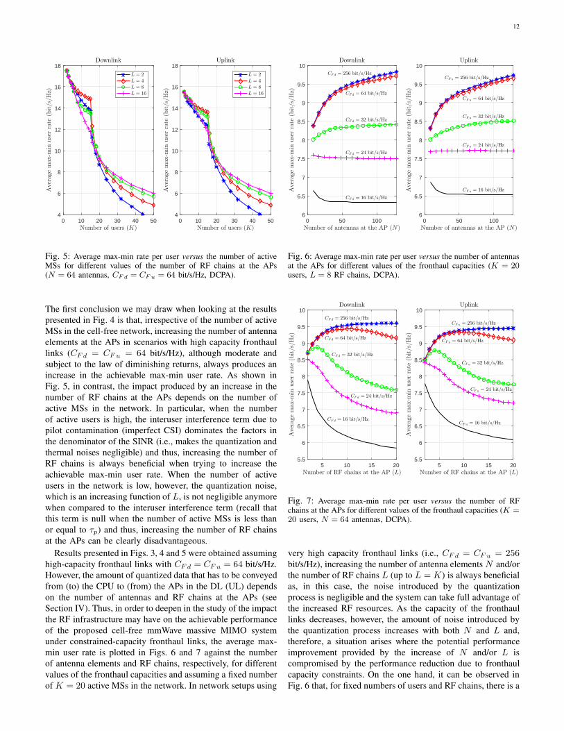
5 10 15 20Number of RF chains at the AP (L)

5.5

6

6.5

7

7.5

8

8.5

9

9.5

10

Average

max

-min

userrate

(bit/s/H

z)

Downlink

CF d = 256 bit/s/Hz

CF d = 64 bit/s/Hz

CF d = 32 bit/s/Hz

CF d = 24 bit/s/Hz

CF d = 16 bit/s/Hz

5 10 15 20Number of RF chains at the AP (L)

5.5

6

6.5

7

7.5

8

8.5

9

9.5

10

Average

max

-min

userrate

(bit/s/H

z)

Uplink

CF u = 256 bit/s/Hz

CF u = 64 bit/s/Hz

CF u = 32 bit/s/Hz

CF u = 24 bit/s/Hz

CF u = 16 bit/s/Hz

Fig. 7: Average max-min rate per user versus the number of RFchains at the APs for different values of the fronthaul capacities (K =

20 users, N = 64 antennas, DCPA).

very high capacity fronthaul links (i.e., CF d = CF u = 256bit/s/Hz), increasing the number of antenna elements N and/or

the number of RF chains L (up to L = K) is always beneficial

as, in this case, the noise introduced by the quantization

process is negligible and the system can take full advantage of

the increased RF resources. As the capacity of the fronthaul

links decreases, however, the amount of noise introduced by

the quantization process increases with both N and L and,

therefore, a situation arises where the potential performance

improvement provided by the increase of N and/or L is

compromised by the performance reduction due to fronthaul

capacity constraints. On the one hand, it can be observed in

Fig. 6 that, for fixed numbers of users and RF chains, there is a

13

0 2 4 6 8 10 12 14 16 18 20Max-min user rate (bit/s/Hz)

0

0.2

0.4

0.6

0.8

1Cumulative

distribution

function

Downlink

K = 25 MSs

K = 8 MSs

M = 25 APsM = 50 APsM = 100 APsM = 200 APs

0 2 4 6 8 10 12 14 16 18 20Max-min user rate (bit/s/Hz)

0

0.2

0.4

0.6

0.8

1

Cumulative

distribution

function

Uplink

K = 25 MSs

K = 8 MSs

M = 25 APsM = 50 APsM = 100 APsM = 200 APs

Fig. 8: CDF of the DL and UL achievable max-min rate per user for different values of the number of APs and active MSs in the cell-freenetwork (N = 64 antennas, L = 8 RF chains, CF d = CF u = 64 bit/s/Hz, DCPA).

certain fronthaul capacity constraint value (near 24 bit/s/Hz in

the setup used in this experiment) under which increasing the

number of antenna elements at the array is counterproductive.

On the other hand, results presented in Fig. 7 show that, for

fixed numbers of users and antenna elements at the arrays,

there is always an optimal number of RF chains to be deployed

(or activated) at the APs that is dependent on the capacity of

the fronthaul links. In particular, for the network setups under

consideration, the optimal number of RF chains is equal to

L = 10, 4, and 1 when using fronthaul links with a capacity of

64 bit/s/Hz, 32 bit/s/Hz and less than 24 bit/s/Hz, respectively.

C. Impact of the density of APs

With the aim of evaluating the impact the density of APs

per area unit may have on the performance of the proposed

cell-free mmWave massive MIMO system, Fig. 8 represents

the cumulative distribution function (CDF) of the DL and

UL achievable max-min user rate for different values of the

number of APs in the network. It has been assumed in these

experiments a fixed number of active MSs equal to either

K = 25 or K = 8 MSs, the use of L = 8 RF chains fully-

connected to a linear uniform antenna array with N = 64antenna elements, and the use of DL and UL fronthaul links

with a capacity CF d = CF u = 64 bit/s/Hz. As expected,

cell-free massive MIMO scenarios with a high density of

APs per area unit significantly outperform those with a low

density of APs per area unit in both median and 95%-likely

achievable per-user rate performance. However, the achievable

max-min user rate increase due to increasing the number of

APs in the network is, again, subject to the law of diminishing

returns. For instance, in scenarios with K = 25 MSs, the

95%-likely achievable user rate is equal to 2.55, 4.33, 6.11

and 6.50 bit/s/Hz for cell-frre massive MIMO networks with

M = 25, 50, 100 and 200 APs, respectively. That is, doubling

the number of APs per area unit does not result in doubling

the 95%-likely achievable user rate. Similar conclusions can

be drawn when looking at either the median or the average

achievable user rates.

As was observed in results presented in previous subsections

for high-capacity fronthaul setups, when the number of active

users in the system is low, the achievable max-min rate values

in the DL are slightly higher than those achievable in the

UL. Instead, when the number of active users increases, the

achievable max-min user rates are virtually identical in both

the DL and the UL. Also, note that the dispersion of the

achievable max-min user rates around the median tends to

diminish as the density of APs increases. That is, cell-free

massive MIMO networks with a high density of APs per

area unit tend to offer max-min achievable rates that suffer

little variations irrespective of the location of the APs (i.e,

irrespective of the scenario under evaluation).

VIII. CONCLUSION

A novel analytical framework for the performance analysis

of cell-free mmWave massive MIMO networks has been intro-

duced in this paper. The proposed framework considers the use

of low-complexity hybrid precoders/decoders where the RF

high-dimensionality phase shifter-based precoding/decoding

stage is based on large-scale second-order channel statistics,

while the low-dimensionality baseband multiuser MIMO pre-

coding/decoding stage can be easily implemented by standard

ZF signal processing schemes using small-scale estimated CSI.

Furthermore, it also takes into account the impact of using

capacity-constrained fronthaul links that assume the use of

large-block lattice quantization codes able to approximate a

Gaussian quantization noise distribution, which constitutes an

upper bound to the performance attained under any practical

quantization scheme. Max-min power allocation and fronthaul

quantization optimization problems have been posed thanks to

the development of mathematically tractable expressions for

both the per-user achievable rates and the fronthaul capacity

consumption. These optimization problems have been solved

by combining the use of block coordinate descent methods

with sequential linear optimization programs. Results have

shown that the proposed DCPA suboptimal pilot allocation

strategy, which is based on the idea of clustering by dissim-

ilarity, overcomes the computational burden of the optimal

14

small-scale CSI-based pilot allocation scheme while clearly

outperforming the pure random and balanced random schemes.

It has also been shown that, although increasing the fronthaul

capacity and/or the density of APs per area unit is always

beneficial from the point of view of the achievable max-min

user rate, the marginal increment of performance produced by

each new increment of these parameters suffers from the law of

diminishing returns, especially for network setups with a high

number of active MSs. Moreover, simulation results indicate

that, as the capacity of the fronthaul links decreases, the

potential performance improvement provided by the increase

of the number of antenna elements N and/or the number of RF

chains L is compromised by the performance reduction due to

the corresponding increase of the fronthaul quantization noise.

In particular, for fixed numbers of users and RF chains, there is

a certain fronthaul capacity constraint value (near 24 bit/s/Hz

in the setups under consideration) under which increasing the

number of antenna elements at the array is counterproductive.

Similarly, for fixed numbers of users and antenna elements at

the arrays, there is always an optimal number of RF chains

to be deployed (or activated) at the APs that is dependent on

the capacity of the fronthaul links. For future work, it would

be interesting to develop low-complexity pilot- and power-

allocation techniques specifically designed to maximize the en-

ergy efficiency of cell-free mmWave massive MIMO networks

considering both the fronthaul capacity constraints and the

fronthaul power consumption. It would also be interesting to

explore the use of partially-connected RF precoding/decoding

architectures and the implementation of baseband MU-MIMO

precoding/decoding other than the ZF scheme.

APPENDIX A

PROOF OF THEOREM 1

Following an approach similar to that proposed by Nayebi

et al. in [17], the signal received by the kth MS in (29) can

be rewritten as ydk = ydk 0 + ydk 1 + ydk 2 + ndk, where the

useful, interuser interference, and quantization noise terms can

be expressed as ydk 0 =√υksdk, ydk 1 = gT

kWBBd Υ

1/2sd,

and ydk 2 = gTk qd =

∑Mm=1 g

Tkmqdm, respectively. Now, con-

sidering that data symbols, quantization noise, thermal noise,

and channel-related coefficients are mutually independent, the

terms ydk 0, ydk 1, ydk 2 and ndk are mutually uncorrelated

and thus, based on the worst-case uncorrelated additive noise

[40], the achievable DL rate for user k is lower bounded by

Rdk = log2 (1 + SINRdk), with

SINRdk =E

|ydk 0|2

E

|ydk 1|2

+ E

|ydk 2|2

+ σ2d

,

where E

|ydk 0|2

= υk,

E

|ydk 1|2

= E

sHd Υ1/2WBB

d

Hg∗kg

Tk W

BBd Υ

1/2sd

= tr(

ΥE

WBBd

Hg∗kg

TkW

BBd

)

=K∑

k′=1

υk′

[

diag(

E

WBBd

Hg∗kg

TkW

BBd

)]

k′

,

and

E

|ydk 2|2

=

M∑

m=1

E

qdHmg∗

kmgTkmqdm

=

M∑

m=1

σ2qdm

tr(

RRFmk

)

.

APPENDIX B

PROOF OF THEOREM 2

The detected signal at the CPU corresponding to the

symbol transmitted by the kth MS in (35) can be rewrit-

ten as yuk = yuk 0 + yuk 1 + yuk 2 + yuk 3, where the

useful, interuser interference, quantization noise and thermal

noise terms can be expressed as yuk 0 =√Pu

√ωksuk,

yuk 1 =√Pu

[

WBBu GΩ

1/2su

]

k, yuk 2 =

[

WBBu qu

]

k, and

yuk 3 =[

WBBu nu

]

k, respectively. As in the DL, since

data symbols, quantization noise, thermal noise, and channel-

related coefficients are mutually independent, the terms yuk 0,

yuk 1, ydk 2 and ydk 3 are mutually uncorrelated and thus,

based on the worst-case uncorrelated additive noise [40],

the achievable UL rate for user k is lower bounded by

Ruk = log2 (1 + SINRuk), with

SINRuk =E

|ydk 0|2

E

|ydk 1|2

+ E

|ydk 2|2

+ E

|ydk 3|2 ,

where E

|yuk 0|2

= Puωk,

E

|yuk 1|2

= PuE

sHu Ω1/2G

HwBB

uk

HwBB

uk GΩ1/2su

= Pu tr(

ΩE

GHwBB

uk

HwBB

uk G)

= Pu

K∑

k′=1

ωk′

[

diag(

E

GHwBB

uk

HwBB

uk G)]

k′

,

with wBBuk denoting the kth row of WBB

u , or, equivalently,

E

|yuk 1|2

= Pu

[

diag(

E

WBBu GΩG

HWBB

u

H)]

k

= Pu

K∑

k′=1

ωk′

[

diag(

E

WBBu gk′ g

Hk′W

BBu

H)]

k,

and, finally,

E

|yuk 2|2

=[

diag(

E

WBBu quq

Hu WBB

u

H)]

k

=

M∑

m=1

[

diag(

E

WBBu qumqH

umWBBu

H)]

k

=

M∑

m=1

σ2q um

[

diag(

E

WBBumWBB

um

H)]

k,

and, analogously,

E

|ydk 3|2

= σ2u(N)

M∑

m=1

[

diag(

E

WBBumWBB

um

H)]

k.

15

REFERENCES

[1] M. Shafi, A. F. Molisch, P. J. Smith, T. Haustein, P. Zhu, P. D. Silva,F. Tufvesson, A. Benjebbour, and G. Wunder, “5G: A tutorial overviewof standards, trials, challenges, deployment, and practice,” IEEE Journal

on Selected Areas in Communications, vol. 35, no. 6, pp. 1201–1221,June 2017.

[2] K. David and H. Berndt, “6G vision and requirements: Is there any needfor beyond 5G?” IEEE Vehicular Technology Magazine, vol. 13, no. 3,pp. 72–80, Sept 2018.

[3] T. L. Marzetta, E. G. Larsson, H. Yang, and H. Q. Ngo, Fundamentals

of massive MIMO. Cambridge University Press, 2016.

[4] T. L. Marzetta, “Noncooperative cellular wireless with unlimited num-bers of base station antennas,” IEEE Transactions on Wireless Commu-

nications, vol. 9, no. 11, pp. 3590–3600, November 2010.

[5] M. K. Karakayali, G. J. Foschini, and R. A. Valenzuela, “Networkcoordination for spectrally efficient communications in cellular systems,”IEEE Wireless Communications, vol. 13, no. 4, pp. 56–61, Aug 2006.

[6] D. Gesbert, S. Hanly, H. Huang, S. S. Shitz, O. Simeone, and W. Yu,“Multi-cell MIMO cooperative networks: A new look at interference,”IEEE Journal on Selected Areas in Communications, vol. 28, no. 9, pp.1380–1408, December 2010.

[7] R. Irmer, H. Droste, P. Marsch, M. Grieger, G. Fettweis, S. Brueck,H. Mayer, L. Thiele, and V. Jungnickel, “Coordinated multipoint:Concepts, performance, and field trial results,” IEEE Communications

Magazine, vol. 49, no. 2, pp. 102–111, February 2011.

[8] A. Checko, H. L. Christiansen, Y. Yan, L. Scolari, G. Kardaras, M. S.Berger, and L. Dittmann, “Cloud RAN for mobile networks - Atechnology overview,” IEEE Communications Surveys Tutorials, vol. 17,no. 1, pp. 405–426, Firstquarter 2015.

[9] H. Q. Ngo, A. Ashikhmin, H. Yang, E. G. Larsson, and T. L. Marzetta,“Cell-free massive MIMO: Uniformly great service for everyone,” inIEEE SPAWC 2015.

[10] ——, “Cell-free massive MIMO versus small cells,” IEEE Transactions

on Wireless Communications, vol. 16, no. 3, pp. 1834–1850, 2017.

[11] T. S. Rappaport, S. Sun, R. Mayzus, H. Zhao, Y. Azar, K. Wang, G. N.Wong, J. K. Schulz, M. Samimi, and F. Gutierrez, “Millimeter wavemobile communications for 5G cellular: It will work!” IEEE Access,vol. 1, pp. 335–349, May 2013.

[12] F. Boccardi, R. W. Heath, A. Lozano, T. L. Marzetta, and P. Popovski,“Five disruptive technology directions for 5G,” IEEE Communications

Magazine, vol. 52, no. 2, pp. 74–80, February 2014.

[13] M. R. Akdeniz, Y. Liu, M. K. Samimi, S. Sun, S. Rangan, T. S.Rappaport, and E. Erkip, “Millimeter wave channel modeling andcellular capacity evaluation,” IEEE Journal on Selected Areas in Com-

munications, vol. 32, no. 6, pp. 1164–1179, 2014.

[14] T. S. Rappaport, Y. Xing, G. R. MacCartney, A. F. Molisch, E. Mellios,and J. Zhang, “Overview of millimeter wave communications for fifth-generation (5G) wireless networks - with a focus on propagationmodels,” IEEE Transactions on Antennas and Propagation, vol. 65,no. 12, pp. 6213–6230, Dec 2017.

[15] X. Gao, L. Dai, and A. M. Sayeed, “Low RF-complexity technologies toenable millimeter-wave MIMO with large antenna array for 5G wirelesscommunications,” IEEE Communications Magazine, vol. 56, no. 4, pp.211–217, April 2018.

[16] S. A. Busari, K. M. S. Huq, S. Mumtaz, L. Dai, and J. Rodriguez,“Millimeter-wave massive MIMO communication for future wirelesssystems: A survey,” IEEE Communications Surveys Tutorials, vol. 20,no. 2, pp. 836–869, Second quarter 2018.

[17] E. Nayebi, A. Ashikhmin, T. L. Marzetta, H. Yang, and B. D. Rao,“Precoding and power optimization in cell-free massive MIMO sys-tems,” IEEE Transactions on Wireless Communications, vol. 16, no. 7,pp. 4445–4459, July 2017.

[18] L. D. Nguyen, T. Q. Duong, H. Q. Ngo, and K. Tourki, “Energy effi-ciency in cell-free massive MIMO with zero-forcing precoding design,”IEEE Communications Letters, vol. 21, no. 8, pp. 1871–1874, Aug 2017.

[19] H. Q. Ngo, L. Tran, T. Q. Duong, M. Matthaiou, and E. G. Larsson,“On the total energy efficiency of cell-free massive MIMO,” IEEE

Transactions on Green Communications and Networking, vol. 2, no. 1,pp. 25–39, March 2018.

[20] M. Bashar, K. Cumanan, A. G. Burr, H. Q. Ngo, and M. Deb-bah, “Cell-free massive MIMO with limited backhaul,” arXiv preprintarXiv:1801.10190, 2018.

[21] M. N. Boroujerdi, A. Abbasfar, and M. Ghanbari, “Cell free massiveMIMO with limited capacity fronthaul,” Wireless Personal Communica-

tions, October 2018.

[22] O. E. Ayach, S. Rajagopal, S. Abu-Surra, Z. Pi, and R. W. Heath,“Spatially sparse precoding in millimeter wave MIMO systems,” IEEETransactions on Wireless Communications, vol. 13, no. 3, pp. 1499–1513, March 2014.

[23] X. Gao, L. Dai, S. Han, C. I, and R. W. Heath, “Energy-efficient hybridanalog and digital precoding for mmWave MIMO systems with largeantenna arrays,” IEEE Journal on Selected Areas in Communications,vol. 34, no. 4, pp. 998–1009, April 2016.

[24] A. F. Molisch, V. V. Ratnam, S. Han, Z. Li, S. L. H. Nguyen, L. Li, andK. Haneda, “Hybrid beamforming for massive MIMO: A survey,” IEEE

Communications Magazine, vol. 55, no. 9, pp. 134–141, Sept 2017.[25] S. Park, A. Alkhateeb, and R. W. Heath, “Dynamic subarrays for hybrid

precoding in wideband mmWave MIMO systems,” IEEE Transactionson Wireless Communications, vol. 16, no. 5, pp. 2907–2920, May 2017.

[26] M. Alonzo and S. Buzzi, “Cell-free and user-centric massive MIMOat millimeter wave frequencies,” in IEEE International Symposium on

Personal, Indoor, and Mobile Radio Communications (PIMRC), Oct2017, pp. 1–5.

[27] M. Alonzo, S. Buzzi, and A. Zappone, “Energy-efficient downlinkpower control in mmwave cell-free and user-centric massiveMIMO,” CoRR, vol. abs/1805.05177, 2018. [Online]. Available:http://arxiv.org/abs/1805.05177

[28] M. K. Samimi and T. S. Rappaport, “Ultra-wideband statistical channelmodel for non line of sight millimeter-wave urban channels,” in 2014IEEE Global Communications Conference, Dec 2014, pp. 3483–3489.

[29] A. Adhikary, E. A. Safadi, M. K. Samimi, R. Wang, G. Caire, T. S.Rappaport, and A. F. Molisch, “Joint spatial division and multiplexingfor mm-Wave channels,” IEEE Journal on Selected Areas in Communi-

cations, vol. 32, no. 6, pp. 1239–1255, June 2014.[30] R. Mendez-Rial, N. Gonzalez-Prelcic, and R. W. Heath, “Adaptive

hybrid precoding and combining in MmWave multiuser MIMO systemsbased on compressed covariance estimation,” in IEEE 6th International

Workshop on Computational Advances in Multi-Sensor Adaptive Pro-

cessing (CAMSAP), Dec 2015, pp. 213–216.[31] S. Park and R. W. Heath, “Spatial channel covariance estimation

for mmWave hybrid MIMO architecture,” in Asilomar Conference on

Signals, Systems and Computers, Nov 2016, pp. 1424–1428.[32] S. Park and R. W. Heath Jr, “Spatial channel covariance estimation for

the hybrid MIMO architecture: A compressive sensing based approach,”arXiv preprint arXiv:1711.04207, 2017.

[33] S. Park, J. Park, A. Yazdan, and R. W. Heath, “Exploiting spatial channelcovariance for hybrid precoding in massive MIMO systems,” IEEE

Transactions on Signal Processing, vol. 65, no. 14, pp. 3818–3832, July2017.

[34] R. Mai, T. Le-Ngoc, and D. H. N. Nguyen, “Two-timescale hybridRF-baseband precoding with MMSE-VP for multi-user massive MIMObroadcast channels,” IEEE Transactions on Wireless Communications,vol. 17, no. 7, pp. 4462–4476, July 2018.

[35] Z. Shen, R. Chen, J. G. Andrews, R. W. Heath, and B. L. Evans, “Lowcomplexity user selection algorithms for multiuser MIMO systems withblock diagonalization,” IEEE Transactions on Signal Processing, vol. 54,no. 9, pp. 3658–3663, 2006.

[36] O. Elijah, C. Y. Leow, T. A. Rahman, S. Nunoo, and S. Z. Iliya, “Acomprehensive survey of pilot contamination in massive MIMO-5Gsystem,” IEEE Comm. Surv. & Tutor., vol. 18, no. 2, pp. 905–923, 2016.

[37] L. Lu, G. Y. Li, A. L. Swindlehurst, A. Ashikhmin, and R. Zhang, “Anoverview of massive MIMO: Benefits and challenges,” IEEE Journal of

Selected Topics in Signal Processing, vol. 8, no. 5, pp. 742–758, 2014.[38] R. Zamir and M. Feder, “On lattice quantization noise,” IEEE Transac-

tions on Information Theory, vol. 42, no. 4, pp. 1152–1159, Jul 1996.[39] G. Femenias and F. Riera-Palou, “Multi-layer downlink precoding for

cloud-RAN systems using full-dimensional massive MIMO,” IEEE

Access, vol. 6, pp. 61 583–61 599, 2018.[40] B. Hassibi and B. M. Hochwald, “How much training is needed in

multiple-antenna wireless links?” IEEE Transactions on Information

Theory, vol. 49, no. 4, pp. 951–963, April 2003.[41] H. Yang and T. L. Marzetta, “Capacity performance of multicell large-

scale antenna systems,” in 51st Annual Allerton Conference on Commu-

nication, Control, and Computing (Allerton), Oct 2013, pp. 668–675.[42] G. Interdonato, H. Q. Ngo, E. G. Larsson, and P. Frenger, “On the perfor-

mance of cell-free massive MIMO with short-term power constraints,”in IEEE 21st International Workshop on Computer Aided Modelling and

Design of Communication Links and Networks (CAMAD), Oct 2016, pp.225–230.

[43] T. M. Cover and J. A. Thomas, Elements of Information Theory (Wiley

Series in Telecommunications and Signal Processing), 2nd ed. Wiley-Interscience, 2006.

16

[44] H. Ahmadi, A. Farhang, N. Marchetti, and A. MacKenzie, “A gametheoretic approach for pilot contamination avoidance in massive MIMO,”IEEE Wireless Communications Letters, vol. 5, no. 1, pp. 12–15, 2016.

[45] P. Tseng, “Convergence of a block coordinate descent method fornondifferentiable minimization,” Journal of Optimization Theory and

Applications, vol. 109, no. 3, pp. 475–494, June 2001.[46] A. Beck and L. Tetruashvili, “On the convergence of block coordinate

descent type methods,” SIAM Journal on Optimization, vol. 23, no. 4,pp. 2037–2060, 2013.