Pedestrian Volume Studies - Chalmers Publication …publications.lib.chalmers.se/records/fulltext/141801.pdfresearch could be performed in subjects such as origin-destination surveys,

Pedestrian Volume Studies

A case study in the city of Gothenburg

Master of Science Thesis in the Master’s Programme Geo and Water Engineering

EDWARDS A. SANTANA MIRANDA

JORGE G. YANNIE CARRASCO

Department of Civil and Environmental Engineering

Division of GeoEngineering

Road and Traffic Group

CHALMERS UNIVERSITY OF TECHNOLOGY

Göteborg, Sweden 2011

Master’s Thesis 2011:12

Master’s Thesis 2011:12

Pedestrian Volume Studies

A case study in the city of Gothenburg







Chalmers University of Technology


Pedestrian Volumes Studies: A case study in the city of Gothenburg, Sweden.




© DEPARTMENT OF CIVIL AND ENVIRONMENTAL ENGINEERING, 2011

Examensarbete / Institutionen för bygg- och miljöteknik,

Chalmers tekniska högskola 2011:12





SE-412 96 Göteborg

Sweden

Telephone: + 46 (0)31-772 1000

Cover:

A representation of pedestrian activities in the city.

Chalmers reproservice / Department of Civil and Environmental Engineering


I

Pedestrian Volumes Studies: A case study in the city of Gothenburg, Sweden.








Abstract

Today, non-motorized traffic is getting more attention due to the lack of knowledge

on this specific subject and the new shift to sustainable development. According to the

literature review, general and established guidelines for pedestrians’ studies do not

exist. In this respect, the purpose of this study was to build up a basis for further

studies related to pedestrians and to develop a methodology for counting them. Using

the established methodology, the counts of pedestrians were performed using three

different methods: manual counting, automatic counting and video counting.

The case study was performed in two streets located in a highly commercial zone in

the centre of the city of Gothenburg: Drottninggantan and Kyrkogatan. The methods

were all applied for these streets to obtain data of pedestrians. The obtained data was

used to generate general statistics of the area (e.g. percentages of genders, volume

directions, ages, etc.), create volume patterns and develop a model to find the optimal

short count (e.g. 5 min, 10 min, 15 min, etc.) to expand it to hourly volumes.

Furthermore, the data was used to calculate expansion factors, calculate the errors of

the automatic devices used to get the data and also to make conclusions about how

each counting method was performed.

The automatic devices were good indicators of the volume patterns of each day.

However, the percentage errors in the volumes were considerable for these devices

and must be taken into account to assess the accuracy of the results. Video counting

was the most reliable counting methodology followed up by the manual counting. The

streets measured had the same land-use and the volume proportions for each section

of the streets were similar but they had small variations which could be attributed to

errors in the automatic counters and to the intrinsic variations that could exist in each

street. The model resulted in that larger sample intervals short counts account better

for the variability of the volumes within the hour sampled.

Further studies are recommended because of the limitations of this study. Future

research could be performed in subjects such as origin-destination surveys, use of

other counting technologies, among others.

Key words: pedestrian counting, pedestrian volumes, pedestrian studies, pedestrian

methodology, estimating pedestrians, short-counts pedestrians, measure pedestrian

and counting non-motorized traffic.

II

CHALMERS, Civil and Environmental Engineering, Master’s Thesis 2011:12

Contents

ABSTRACT I

CONTENTS II

PREFACE IV

NOTATIONS V

1 INTRODUCTION 1

1.1 Background 1

1.2 Aim 2

1.3 Method 2

1.4 Limitations 3

2 LITERATURE REVIEW 4

2.1 Pedestrian volumes studies 4

2.2 Volume characteristics 4

2.2.1 Time-of-day variation 5 2.2.2 Daily variation 6

2.2.3 Monthly or seasonal variation 7 2.2.4 Directional variation 8 2.2.5 Geographical variation 8

2.2.6 Weather variation 9

2.3 Volumes within the hour 9

2.4 Field methods for measuring pedestrian volumes 10 2.4.1 Manual counts 10

2.4.2 Automatic counts 10 2.4.3 Counting periods 11 2.4.4 Sampling and sampling theory 12

2.5 Specific volume studies 13 2.5.1 Screen-line counts 13

2.5.2 Limited network volume study 13

3 METHODOLOGY 16

3.1 Site description 16

3.2 Manual counts 19 3.2.1 Sampling 20

3.2.2 Data log 20 3.2.3 Days counted 20

3.2.4 Weeks counted 21 3.2.5 Equipment used 22 3.2.6 During the counting period 24 3.2.7 Personnel 24

III

CHALMERS Civil and Environmental Engineering, Master’s Thesis 2011:12

3.3 Automatic counters 24

3.4 Video counting 26

4 RESULTS 28

4.1 General statistics 28

4.1.1 Pedestrians’ volumes on each sidewalk 28 4.1.2 Walking direction 29 4.1.3 Classification by gender 32 4.1.4 Classification by age 33

4.2 Automatic counter accuracy 34

4.3 Volume Pattern 40

4.4 Data analysis 44

4.5 Model 47

4.6 Example calculation 51

5 SUMMARY AND DISCUSSION 54

6 CONCLUSIONS 57

7 RECOMMENDATIONS 59

7.1 Future Research 59

REFERENCES 60

APPENDIX 1 – VOLUME PROPORTIONS FOR EACH DAY AND SECTION 63

APPENDIX 2 – VOLUMES OBTAINED WITH THE MANUAL COUNTS 65

APPENDIX 3 – SITE SETUP 68

IV


Preface

During the development of this research, several methodologies are applied for

counting pedestrians in two streets of the city of Gothenburg. The task is part of

measuring the actual volumes of pedestrians walking in the city centre of Gothenburg.

The project is carried out from September 2010 to February 2011 at the Department

of Civil and Environmental Engineering, GeoEngineering division, Chalmers

University of Technology and at the Traffic and Public Transport Authority of

Gothenburg.

The project has been carried with Edwards Santana and Jorge Yannie as researchers,

Professor Gunnar Lannér as examiner-supervisor and Anna-Lena Lindström as

supervisor. All the materials used to develop and apply the methodologies are

supplied by the Department of Civil and Environmental Engineering, GeoEngineering

division, Chalmers University of Technology. We would like to thank Gunnar Lannér

and Anna-Lena Lindström for their help and enriching comments and ideas. In

addition, we express gratitude to Thomas Jonsson, David von Martens, Annika

Nilsson, Marleny Lora, Ivannia Santana, Karin Björklind, Max Falk, Laura Lelliot,

and the whole planning department of the Gothenburg’s Traffic and Public Transport

Authority for their help and involvement. In addition, we would like to thank Vectura

Consulting AB for their contribution in the project by supplying us with the data from

the automatic counters.

This project could have never been conducted without the help of Orlando Mezquita,

a close friend from the Dominican Republic, who guided us through the statistical

analysis of the obtained data. Finally, we would like to specially thank our family and

friends for the support and help throughout the development of this research.

Göteborg February 2011

Edwards Santana

Jorge Yannie

Jorge Yannie:

“By observation one can define the underpinning patterns of things on Earth”.

V

CHALMERS Civil and Environmental Engineering, Master’s Thesis 2011:12

Notations

α-value The probability of rejecting the null hypothesis when the latter is true.

Adjustment factor for day “i”.

Expansion hourly factor; for the specific hour “i” of study.

Expansion hourly factor for the peak hour.

Number of pedestrians considered to be real (e.g. manual or video

counts).

Number of pedestrians counted by the automatic counter or field

observers.

Number of periods within the hour.

p-value Indicates how well the sample evidence supports the decision to reject

the null hypothesis.

PHF Peak hour factor

R2(adjusted) R

2 adjusted for the number of explanatory terms in a model.

R2(predicted)

The proportion of the total variation in Y that is accounted for by the

predictor variable X.

S Residual standard deviation.

Average volume for the counted days in the control counts;

pedestrians. (e.g. average for all Mondays, all weekdays, etc.).

Adjusted volume representing an average of the days counted in the

control counts study period, pedestrians (e.g. average volume for

Mondays of month “x”).

Coverage count volume for the same hour as the EHF, pedestrians.

Volume for day “i” from the coverage/short counts, pedestrians (could

be Ve).

Specific study day “i” volume from the control count study period;

pedestrians (“i” represent each day individually counted, e.g. Monday

1, Monday 2, Tuesday 1, Tuesday 2, etc.).

Total volume expanded for the sample link, pedestrians.

Specific study hour “i” volume from the control count, pedestrians.

VI


Maximum volume for a “n” minutes period (e.g. 5 or 15 minutes, Vm5

or Vm15) within the hour, pedestrians.

Peak hour volume, pedestrians.

Total volume from the control count for the full sampling period,

pedestrians.

1


1 Introduction

The following chapter gives information of the background, aim, methods and

limitations in the work. The study was performed on two streets of the city centre of

Gothenburg and it is mainly related to pedestrian volumes studies.

1.1 Background

The city of Gothenburg is in a “state of change” in respect of its urban composition; it

is growing and with it comes the necessity of a better transportation system. Growth

in the transportation system can be related to environmental impacts and risk of more

accidents if improper measures are taken. In these days, politicians are aware of these

facts and have created new aims to avoid the latter. New projects have been

developed, for example the K2020 with aiming to develop the public transport in the

city and the Vision Zero project which targets to have no serious injured in the traffic

environment. As a direct consequence the public transportation has to face a major

reformation.

The Gothenburg public transport is a very versatile system in respect to the different

modes of transportation. It is mainly composed by busses, trams, commuter trains and

ferries (motorized modes). In addition, these modes are all interconnected by bicycles

and pedestrians routes, making the whole system an interrelated unit.

The transportation field is a very broad field and during these last years it has been

well documented, primarily in respect to motorized modes. However, non-motorized

modes have been deemed as “less important”, as observed with the scarce information

available today. A big obstacle facing the non-motorized field is the poor amount of

documentation on usage and demand. This information is important to account for the

benefits of projects related to these forms of transportation and to be able to evaluate

them against other modes, for example private vehicles (Ragland & Jones, 2010).

Little attention was paid to the pedestrians until recent years; result of stringent safety

regulations and a shift to sustainable development, see Figure 1. Today non-motorized

transit is getting more attention; exemplified by the project conducted by the

Gothenburg’s Traffic and Public Transport Authority in Drottninggatan and

Kyrkogatan, two important streets located in the city centre of Gothenburg. The

streets’ life in this particular area is characterized by being constantly active. This is

an attractive area for pedestrians due to its availability of shops, restaurants and cafes

where people can spend their day. Furthermore, they are important transportation

corridors for non-motorized traffic.

2


Figure 1. Modal split of the city of Gothenburg and Stockholm as a measure of sustainability (Urban

Audit, 2004).

In general the city of Gothenburg is lacking information about the traffic of

pedestrians. At the moment, more studies are being carried out due to the lack of

knowledge on the behaviour and volume of pedestrians walking on the streets. One

example that required pedestrian data was the study performed by Jonsson (2005)

about predictive models for accidents on urban links involving vulnerable road users.

Another is the investigation done by Niska et al. (2010) about the measures and

methods for evaluating pedestrian and bicycle traffic.

1.2 Aim

The main purpose of this research is to build up a basis for further studies related to

pedestrian volumes. One target is to evaluate methodologies for obtaining pedestrians

volumes and how they could be more efficient. Three different approaches are

assessed, manual, automatic and video counting; each of them having their own

advantages and disadvantages, as further presented.

In addition, a comparison is done between the volumes obtained from applying the

manual counting methodology and the automatic counters. The accuracy of the

methodology and the extent of the validity of the undertaken assumptions are

evaluated. Regression models are used to determine an efficient short count interval in

order to save resources when performing a manual count sampling.

1.3 Method

The search for information was made using resources from the library of Chalmers

University of Technology, databases such as the VTI’s Transguide and TRIS. In

addition, the use of online search engines was helpful to obtain scientific publications

in the field. Key words used during the search were: pedestrian volumes, estimating

62%

48%

12%

6% 10% 11%

15%

34%

Göteborg Stockholm

Sustainability Measure

Private Vehicles

Cycling

Walking

Public transport (rail,metro, bus, tram)

3


pedestrians, pedestrian studies, pedestrian counting, and counting non-motorized

traffic.

Data collecting was performed by the researchers themselves, in relation to manual

and video counting. Automatic counters were supplied by Vectura Consulting AB. In

addition, data analysis was performed by the help of softwares like Microsoft Excel,

Minitab 16 and MathCAD.

1.4 Limitations

The investigation was focused on specific streets of the city centre of Gothenburg;

namely Drottninggatan and Kyrkogatan. Both streets are within the same land use

(commercial area) and they reflect similar characteristics, limiting the ability to relate

the results to other land uses (i.e. residential areas, recreational areas, etc.).

Manual counting was performed in hours within the range of 12.00-18.00 due to time

restrictions. A complete day or more than two straight hours were not manually

counted. The complete study was performed for 2 months, only accounting for daily

and weekly variations.

Most of the theory was derived from motorized traffic modes and modified as needed

to fit non-motorized modes. The latter was due to the lack of documentation on

pedestrians’ studies.

4


2 Literature review

The literature review helps to give the reader an insight of the main concepts related

to pedestrian volume studies. In addition, it revealed the scarce information available

on this topic. The major part of the accessible information was related to studies

conducted in the United States. Furthermore, most of the documented theory related

to volume studies is from motorized traffic.

2.1 Pedestrian volumes studies

As a way to explain the current status of the transportation system, engineers are

required to collect diverse data and information (Roess, et al., 2004). In this manner,

focus is set in collecting data related to the volume of pedestrians in the system. The

data can have several applications, for example it can help to perform safety analysis

studies, look for modifications in infrastructure, forecast future trends in society,

business development, among others (Schneider, et al., 2008). The collected data is

the basis for obtaining the information needed for the planning, designing and

decision-making processes.

It is important to know the actual behaviour of pedestrians so future projects can be

proper developed. For example, if the pedestrian’s concentration zones are known,

future bus/trams/metro stops could be created in order to distribute better the volumes.

In traffic engineering, volume studies are most of the time needed, for example to

measure demand or usage of pedestrians. Roess, et al. (2004) defines volume as “the

number of persons passing a point during a specified time period”. The observed

volumes can equalize the demand (pedestrian that desired to travel), the capacity of

the studied segment (maximum rate) or none of them (Roess, et al., 2004), see Figure

2.

Figure 2. Demand versus Capacity for pedestrian traffic (modified from Roess, et al., 2004). The output

reflects how the demand is delayed in time, increasing the usage time.

2.2 Volume characteristics

Volume proportion patterns will be the same even though actual volumes can change

in a specific location, unless the site is drastically modified. Garber & Hoel (2002)

300

400

500

600

700

800

0 1 2 3 4

Flo

w r

atio

(P

ed

/hr)

Time (hours)

Demand

Capacity

Output

5


stated that “regular observation of traffic volumes over the years has identified certain

characteristic showing that although traffic volume at a section of a road varies from

time to time, this variation is repetitive and rhythmic”. The demand is not a constant

value; it changes together with the time (i.e. time of day, week, month or year).

Moreover, it can be influenced by external factors (planned or unplanned) such as

accidents, occasional events, detours, or even by the weather (Roess, et al., 2004).

This is affirmed by Schneider, et al., (2008) and Aultman-Hall, et al., (2009), stating

that pedestrian’s activity levels are variable during the day, by location and weather

conditions.

With the help of volume patterns it is possible to develop proper design and control

methods in a certain area (Roess, et al., 2004). According to Roess, et al., (2004), this

is a difficult task for traffic engineers because “planning and designing is usually

made for a demand that represents a peak flow rate within a peak hour on a peak day

during a peak season”. This translates into the necessity of extensive knowledge of the

situation in relation to time.

2.2.1 Time-of-day variation

Traffic changes as the day progresses, e.g. traffic volumes increase during the day and

decrease at night. This behaviour is represented in a time-of-day pattern, where

different patterns can exist within different places (FHWA, 2001), see Figure 3.

6


Figure 3. Two hour volume pattern variation from vehicle traffic, where each bar represent 5 minutes

flow rate (veh/hr). It is expected to obtain similar patterns for pedestrians volumes (modified from

Roess, et al., 2004).

2.2.2 Daily variation

According to Roess, et al., 2004, “daily variation patterns are caused by the type of

land uses and trip purposes”. Patterns will differ during the week, mainly because the

different alternatives activities that can be done in a week; e.g. pedestrians will go

more often to shops on weekends in contrast with weekdays when most of them are

working, running errands or at school. Day-of-week patterns will also vary with land

use, e.g. urban or rural areas, central business district (CBD), downtown, residential

area, etc. (FHWA, 2001), see Figure 4.

7


Figure 4. Day-of-week pattern for some roads in the United States for vehicle traffic. Pedestrians’

volume pattern will present a similar behaviour during the week in relation to other factors, i.e. land

use (modified from Roess, et al., 2004).

2.2.3 Monthly or seasonal variation

Volume patterns will vary during the year according to each season. For example, in

summer most trips have recreational purposes whilst commuters’ trips are less

frequent (Roess, et al., 2004), see Figure 5.

8


Figure 5. Monthly volume pattern variations for vehicle traffic. Once more it is believed that

pedestrian volume pattern will reflect similar behaviour (modified from Roess, et al., 2004).

2.2.4 Directional variation

Most streets exhibit differences in flow by direction. In urban areas, peak traffic can

be seen coming into the city early in the morning but in the afternoon the peaks are in

the traffic that is leaving the city. The patterns can change depending on the use of the

street/road (e.g. where there is recreational traffic) (FHWA, 2001).

2.2.5 Geographical variation

Volume patterns will differ significantly between different places (land uses), mainly

because not all the various activities performed by the users are concentrated in one

area (FHWA, 2001). It has been found in previous studies that pedestrian volume

patterns are site specific (Aultman H., et al., 2009; Turvey, et al., 1987), see Figure 6.

9


Figure 6. To the left, twelve hour volume patterns for different type of land uses (modified from Davis,

et al., 1988) and to the right and illustration of the relation of the pattern with land use.

2.2.6 Weather variation

Severe weather conditions can alter the overall volume pattern within relative short

times, i.e. some hours or even a day. Usually extreme weather conditions are not

presented for long time periods and can be regarded as punctual fluctuations in the

volume patterns.

Aultman-Hall, et al. (2009) found out that there is a weak relation between the

weather and the volume of pedestrians. Furthermore, they discussed that the weather

perception is more a restriction for the pedestrians than the weather itself.

2.3 Volumes within the hour

Facilities are generally designed to fulfil the peak hour demand. However, there are

demands within the hour that reflect a peak that may surpass the capacity and thus

generate a breakdown in the system (Roess, et al., 2004). Roess, et al. (2004) defines

the rate of flow as “the rate at which pedestrians pass a point during a specified time

period less than one hour, expressed as an equivalent hourly rate”.

For the above stated phenomena, the study and design of traffic facilities must be

done for the maximum rate of flow within the peak hour. In general, 15 minutes

periods are used as the base value for the rate of flow. To support the use of 15

minutes time intervals, it is said that collapses of the system for shorter intervals can

dissipate and stabilize rather quickly (Roess, et al., 2004).

The mathematical relationship between the peak hour volume and the maximum rate

of flow within the hour is defined by the peak hour factor (PHF) as follows (Roess, et

al., 2004):

(1)

Peak hour volume, pedestrians.

Maximum volume for a “n” minutes period (e.g. 5 or 15 minutes, Vm5 or

10


Vm15) within the hour, pedestrians.

Number of periods within the hour.

The PHF will tell how variable the volume is within the peak hour, e.g. a value close

to one will represent a nearly constant volume in each time period. With this factor,

the maximum rate of flow can be estimated for the peak hour volume.

2.4 Field methods for measuring pedestrian volumes

Factors like time, land use and weather are taken into account when performing

volume studies. It is frequent to perform measurements within times of high

pedestrian volume (peak hours). In addition, pedestrian counts are performed in good

weather conditions; however there are special cases where the weather variation plays

an important role for the study. The locations at which pedestrian counts are done

include intersections, along sidewalks, and mid-block crossings (Garber & Hoel,

2002).

2.4.1 Manual counts

Manual counts can supply a large set of data if necessary, for example pedestrians’

age, gender, physical handicap and behaviour (Robertson et al., 1994). Furthermore,

they are quickly to set up and perform (Roess, et al., 2004). However, they require a

lot of effort from trained personnel and collecting data manually for long periods

becomes unfeasible due to economical reasons (Greene-Roesel, et al. 2008).

Equipment for manual counts

There are several equipments used to perfom manual counts, for example tally sheets,

hand-counters, board-mounted counters and electronic counters. Tally sheets are most

commonly used in manual counts due to the fact that they provide the possibility to

classify volumes and write observations, plus they are rather cheap.

Personnel consideration

In order to obtain good quality data, all the personnel involved in the study and the

field counting must be aware of the importance of the study and the final outcome that

wants to be reached. A recommendation is to perform trainings on how to use all the

material for the counting procedure, some days before it starts (Roess, et al., 2004). A

study performed by Diogenes, et al. (2006) supports this fact and address it as a

necessary step for obtaining data with good quality.

2.4.2 Automatic counts

Automatic count technologies help to create long-term volume variation patterns in a

more efficient way than manual counting (e.g. they do not require man-hours). The

most common technologies available for counting bicycle and pedestrian are listed in

Table 1. Despite the variable available technology, there is a small amount of

information at hand about the performance and reliability on these devices, especially

on outdoor environments (Greene-Roesel, et al. 2008).

11


Table 1. Most common type of automatic counters in the market (extracted from Ragland & Jones,

2010).

Types of automatic counters

Passive infrared, detects a change in thermal contrast.

Active infrared, detects an obstruction in the ray beam.

Ultrasonic, emits ultrasonic waves and listens for an echo.

Doppler radar, emits radio waves and listens for a change in frequency.

Video imagining, either analyzes pixel changes or data are played back in high speed

and analyzed by a person.

Piezometric, senses pressure on a material either tube or underground sensor.

In-pavement magnetic loop, senses change in magnetic field as metal passes over it.

2.4.3 Counting periods

The counting period depends on the purpose of the study and the equipment available

to perform it. It could be as short as some minutes or as long as a year. The purpose of

the study will tell which days and which specific hours within those days to count

(e.g. typical weekdays from Tuesday to Thursday at peak hours) (Robertson et al.,

1994).

Continuous counts

Continuous counts give information about patterns, basically of a season, a week or a

day. The data obtained with this type of counts is used to calculate adjustment and

expansion factors that transform short counts data into other time range estimates or

design values (FHWA, 2001).

Control-counts

The data obtained from control-counts (or “key counts”) also help to determine

expansion factors. As continuous counts, they provide knowledge about seasonal and

monthly volume variation patterns if set for long times (Garber & Hoel, 2002).

Control-count stations support continuous count stations (Robertson et al., 1994) and

they are established for less time than the continuous counts.

Coverage counts or short counts

These counts are conducted in sample locations where data needs to be gathered and

they are only performed in specific times of the study period (Roess, et al., 2004).

Robertson et al. (1994) stated that “a number of studies that use pedestrian volumes

often required less than 10 hours of data at any given location”. Typical count periods

for pedestrian are (Robertson et al., 1994):

2 hours; peak period.

4 hours; morning and afternoon peak periods.

12


6 hours; morning, midday and afternoon peak periods.

12 hours; daytime (e.g. 7:00-19:00).

Normally, count intervals are 5 or 15 minutes. If capacity analysis is required, a 15

minutes interval is preferable. In the other hand, if the study is based on finding a

critical peak hour factor, 5 minutes can be selected (Robertson et al., 1994).

Several issues such as time and money do not allow performing counts for all the time

periods, which is the reason for conducting short counts. The results from this

counting are adjusted or expanded to know the total volume of pedestrians at the

sampled location. The larger the variation in the volumes of the short count intervals,

the longer the sampling period must be in order to obtain acceptable estimates from

the expansion factors (Robertson et al., 1994).

2.4.4 Sampling and sampling theory

Statistical sampling procedures are generally required to be performed in random

locations in order to avoid bias on the estimated statistics. However, a random

approach is hard to apply due to most of the required data is site-specific (FHWA,

2001).

The amount of samples to take will be related to the level of activity within the

selected location. Alta Planning & Design (2010) recommends 1 to 3 samples. If it is

noticed that in the counting location the activity of pedestrian is high (e.g. 100 ped/hr)

one sample could be sufficient for one weekday and one weekend day. However, if

the volumes are low and the place present irregular activities, 2 or 3 counts should be

performed on continuous days or weeks. Using several counting periods that are 1

week or more apart will preclude any unusual conditions occurring on a given day

from causing a bias in the data (Robertson et al., 1994).

Dates

Alta Planning & Design (2010) suggested that weekdays and weekend days should be

sampled at least one day in order to assess the behaviour of these two time periods.

Furthermore, to prevent skewness or bias of the data caused by different factors,

counts can be performed on more than a weekday or weekend in a successive way.

In general, the best period to perform pedestrian counts is considered to be during

September. This month have the characteristic that all the main activities in a city (i.e.

works, schools, tourism, etc.) are active and that weather conditions are appropriate

for walking (Alta Planning & Design, 2010). Nevertheless, this is a site-specific

characteristic that must be known in advance.

Time

The times for performing the counts are basically used to address the peak periods in

the day. According to Alta Planning & Design (2010) the 12-hour range from 7:00 to

19:00 for both weekdays and weekends are suitable for counting. This time range,

usually accounts for most of the volume of the complete day, however this

characteristic is site-specific and must be evaluated beforehand.

13


2.5 Specific volume studies

A number of specific studies related to traffic volumes can be performed for the

transportation system. A focus is set in two of them, screen-line counts and limited

network volume studies; which are generally combined and performed together.

2.5.1 Screen-line counts

The count consists on creating an imaginary axis perpendicular to the pedestrians’

path, where all pedestrians crossing the line are counted. Screen line counts can help

to identify the movement of people from one place to another (Robertson et al., 1994).

These counts are primarily used to obtain volume patterns and to assess the different

factors that affect walking and bicycling in an area (Ragland & Jones, 2010).

2.5.2 Limited network volume study

When dealing with large networks (i.e. a city central street network), sampling

procedures are applied assuming that the whole network or sub-part of it will have the

same trends of volumes with time. These trends are measured at some locations of the

network and then used for other locations inside it (Roess, et al., 2004), see Figure 7.

The volume studies for limited network can be done in several ways, as explained

below.

Figure 7. To the left, a representation of a limited network. To the right, an illustration of the

correlation by land use.

A one-day study plan

In this method, one control count is set in a representative place to determine the

volume trends of the network (continuous count) and the other streets are measured

(coverage counts) within the time of the study period. Coverage counts are expanded

using the volume patterns from the continuous counts (Roess, et al., 2004).

14


A rule of thumb is that the control station must service the same type of street and

variations of traffic being sample on the other streets. The control count gathers data

for the whole study period. The resulting pattern from these data is quantified by

finding out the proportion of volume for the same time intervals as the coverage

count, in relation to the complete volume of the control count. This proportion is

known as the “expansion factor”. To obtain the complete study period volume (e.g. an

hour, day, month or year) for a coverage count location, one must divide the coverage

count by the expansion factor of the same time interval as it was taken (Robertson et

al., 1994). The mathematical procedure for 1 hour is explained below (the same for

different times in short counts, i.e. 5 or 15 minutes):

(2)


Specific study hour “i” volume from the control count, pedestrians.

Total volume from the control count for the full sampling period,

pedestrians.

(3)



Coverage count volume for the same hour as the EHF, pedestrians.

The largest EHF will represent the peak hour within the time period of study. This

factor can be used to find the peak hour volume for the other links after obtaining

their total volume for the time period of study from expanding the short counts.

Mathematically expressed, it is:

(4)

Peak hour volume for sample link, pedestrians.

Expansion hourly factor for the peak hour.


The expanded data represent the day on which the counts were taken. Daily and

seasonal variations have not been accounted by this technique (Roess, et al., 2004).

A multi-day study plan

Roess, et al. (2004) stated that “hourly variation patterns are not as stable as variations

over larger periods of time”; meaning that is preferable to perform the short counts for

the whole study period (e.g. from 7:00 to 19:00. Nevertheless, if the counts are

15


performed for the whole study period for each link in the network, several days will

be required depending on the amount of resources (e.g. man-working hours). In this

matter, the days will have volume variability and to account for it, adjustment factors

are applied (Roess, et al., 2004). The adjustment factors can account for a specific

day’s average, a weekdays’ average, a weekend’s average, a complete week average

or any other time average. The computation of these factors is shown below:

(5)

Adjustment factor for day “i”.

Average volume for the counted days in the control counts; pedestrians.

(e.g. average for all Mondays, all weekdays, etc.).

Specific study day “i” volume from the control count study period;

pedestrians (“i” represent each day individually counted, e.g. Monday 1,

Monday 2, Tuesday 1, Tuesday 2, etc.).

(6)

Adjusted volume representing an average of the days counted in the

control counts study period, pedestrians (e.g. average volume for

Mondays of month “x”).

Volume for day “i” from the coverage/short counts, pedestrians (could

be Ve).

With this method, the main purpose of the control counts is to obtain daily variation

volume patterns, since the coverage counts are performed for the complete day

accounting for the hourly volume variation. The goal of the adjustment factor is to

regulate the daily variability in order to obtain an average volume for the desired days

within the control count study period. It is good to group days in weekdays and

weekend days if possible, to obtain an average volume for each. Seasonal variations

are not accounted (Roess, et al., 2004).

Mixed approach

When coverage counts could not be performed for the complete day, a mixed

approach can be used. This consists in performing coverage counts for a specific time

interval (e.g. 15 min, 1 hour, etc.) in order to expand the volume for the day. Thus, the

daily volume is adjusted to account for the average of the control count study period.

Again, seasonal variations are not accounted, only daily variation for the days in the

study period (Roess, et al., 2004).

16


3 METHODOLOGY

The literature review has revealed that general and established guidelines for

pedestrians studies do not exist. As an example, Schneider, et al. (2008) stated in their

work that there is not a standard methodology for counting pedestrians. Most of the

theory found is related to motorized traffic; however, more research and efforts to

increase the knowledge of this field and set general guidelines is being done in

different countries. For example in the United States a national program for counting

pedestrians and bicycles is been developed called “The National Bicycle and

Pedestrian Documentation Project” (Alta Planning & Design, 2010) and in Europe,

programs like “Measuring Walking” (Sauter, 2010). In fact, available information is

scarce and very specific.

Having created a standardized methodology sets a basis for future studies.

Furthermore it can help to improve data collection efforts by having a consistent

method that can be compared in time and improved every time it is executed

(Schneider, et al., 2005).

The count of pedestrians was performed using three different methods: manual

counting, automatic counters and video counting. The use of different methods was to

support the result from each of them and to compare the outcomes.

3.1 Site description

The case study was performed in the city of Gothenburg, Sweden. Data collection was

performed in two streets of the city centre, specifically Drottninggatan and

Kyrkogatan. These were selected in accordance to the request of the Gothenburg’s

Traffic and Public Transport Authority to investigate the actual pedestrian volumes, in

order to assess the possibility of making them a shared space between motorized and

non-motorized traffic. The two streets are located in a highly commercial zone, shown

in Figure 8. Both sections are in the east side of Östra Hamngatan, the main avenue of

the city centre of Gothenburg, and intersecting Fredsgatan. The latter street is a

“pedestrian street” and is one of the areas where the majority of the people tended to

walk. This area is characterized by large volumes of pedestrians shopping, eating and

working around.

17


Figure 8. Drottninggatan and Kyrkogatan among the commercial squares of the city centre; counted

sections marked by green lines and surrounded by a square (Eniro, 2010).

Each street was divided in two sections that were numbered according to the counting

sequence (i.e. section 1 was the first counting place). Each section was composed by

two sidewalks, side A and B, which were commonly arcades. The counting points

were governed by the location of the automatic counters, which required a place free

of obstacles, with a clear view and with the adequate height to count every type of

pedestrian. The location of the automatic counters, the field observers, the video

camera and each section of the streets are illustrated in Figure 9 (see Appendix 3 for a

resized figure).

Figure 9. Location of automatic counters, pneumatic tubes, personnel counting and coverage range of

the video camera for each section.

18


The studied segment of Drottninggatan has an approximate length of 200 m and an

average street width of 5.70 m. The measured segment of Kyrkogatan has an

approximate length of 150 m. The widths of the street are 6.30 m and 5.55 m for

section 3 and 4, respectively.

The widths of each sidewalk for all the sections are shown in Table 2; where the

arcades widths are measured as the available space for pedestrian to walk. In this table

can be noticed that the side A is narrow in both sections of Drottninggatan. Side B is

an arcade along the whole segment of this street; see Figure 10 and Figure 11. In the

first section, side B gives the impression of a narrow hallway, since the width is

almost the same as for side A. For the case of Kyrkogatan in section 3, both sidewalks

are arcades, but in section 4, only side A has them.

Table 2. Width of the sidewalks for each street.

Width of sidewalks (m)

Street Section Sidewalk A Sidewalk B

Drottninggatan 1 1.50 1.60

2 1.20 2.65

Kyrkogatan 3 2.40 2.35

4 2.45 1.20

Figure 10. Arcades of section 1 in Drottninggatan. The arcade gives the impression of being inside a

long tunnel.

19


Figure 11. A clear picture showing an arcade in side B in section 2 of Drottninggatan. On the left, the

automatic counter (grey box) can be observed mounted to the pole surrounded by a red square.

3.2 Manual counts

Drottninggatan and Kyrkogatan are part of the city centre network. As stated in

chapter 3.1, the area is a highly commercial zone with a large flow of pedestrians. The

manual count procedure used in this section of the network was a screen-line count.

The screen-line count is basically done by standing at a side of the sidewalk and

counting every pedestrian that passes in each direction over an imaginary line, in this

case along the automatic counter axis as illustrated in Figure 12. The imaginary line

was further illustrated by the use of a yellow line in the ground surface in order to

increase the accuracy and ease of the counting; see Figure 13. However, there were

occasions were the line was drawn by the observers’ eyes.

20


Figure 12. Elements of a counting section.

Figure 13. A yellow tape adhered to the

pavement was used as the indicator for

the imaginary line in the screen-line

counting method.

3.2.1 Sampling

The collection of the field data was made for sample lengths of 1 hour and during

good weather conditions, i.e. a sunny or cloudy day without rain. The hours in which

the counts were performed, were the ones where the peak hour was expected to take

place. It must be stated that some counts were performed for more than an hour, e.g. 2

hours. These hours were selected considering the background information of the place

and previous records where the highest volumes of pedestrians have been observed

(Bladh, et al., 1984). Specifically, the ranges selected were 12:00-13:00 (lunch time)

and 16:00-17:00 (end of daily journeys). Furthermore, other periods of one hour

between 12:00-19:00 were chosen to account for different volume scenarios that could

be compared later on with the automatic counters.

3.2.2 Data log

For each sample period, the log intervals were set to 5 minutes. This small time was

chosen to evaluate variations in the data and as a basis to generate other time

intervals. For example, to compare the manual counts with the automatic counts, the

smaller time interval possible was 15 minutes.

3.2.3 Days counted

The weekdays were used as the main sample days for this study. In this respect,

random days among this group were chosen. From the literature review it was stated

that Tuesdays, Wednesdays and Thursdays are days that are likely to have the same

21


pattern of pedestrian volumes within the week (Alta Planning & Design, 2010).

Mondays and Fridays were sampled as well because these days are supposed to have

different volume patterns (Robertson et al., 1994). A special count was performed on

a Saturday to see how the volume changed from that of the weekdays and to assess

the fact that the area is a commercial zone with expected higher volumes on the

weekends (Robertson et al., 1994).

There are several special days in which it is interesting to know the volume of people

walking. For example, Fridays and Saturdays can be different due to traditional

activities like “afterworks” and due to the night life. However, these days cause a bias

on the volume of pedestrians in comparison to the remaining days of the week;

consequently it is better to count in other days rather than these.

3.2.4 Weeks counted

The manual counts were performed during the same time period for which the

automatic counters were set. The random sampled days and the time in which the

manual counts were performed for each of the streets are shown in Table 3 and Table

4. A total of 27 samples were collected, from which 26 were measured for a whole

hour and 1 for half an hour.

Table 3. Amount of manual counts performed in Drottninggatan.

Drottninggatan

Peak Hour Mon. Tue. Wed. Thu. Fri. Sat. Sun. Total

12:00 - 13:00 1 2* 1 2 6

13:00 - 14:00 2 2

16:00 - 17:00 1 1 1 3

17:00 - 18:00 1 2 3

18:00 – 19:00 1 1

Total 2 5 - 4 4 - - 15

* One of the samples is for half an hour.

22


Table 4. Amount of manual counts performed in Kyrkogatan.

Kyrkogatan

Peak Hour Mon. Tue. Wed. Thu. Fri. Sat. Sun. Total

12:00 - 13:00 3 2 1 6

13:00 - 14:00 1 1

16:00 - 17:00 1 1 1 3

17:00 - 18:00 1 1 2

Total 4 2 2 1 1 2 - 12

3.2.5 Equipment used

The personnel were provided with all the required material to perform a systemized

counting. Some of these included instruction forms, count forms, location map,

clipboards, pen and pencils and time watches.

Tally sheets together with a time watch were used as the main tools for undertaking

the manual counting. The former contained the basic details of the intersection

involved and required information about the observer’s name, day and date of the

count, weather conditions, observer’s location (sidewalk side), time of the count

(starting and ending time) and the location of the counting study. See Figure 14 and

Figure 15 to view the format of the tally sheet used for the counting. The data that was

gathered included:

The walking direction of pedestrians, i.e. heading east or west.

Approximate age; this based on a subjective judgement. Children were

considered to be below 14 years, adults between 14 and 60 years and the

rest as elderly.

Gender.

23


Figure 14. Front page of the tally sheet used. Location, current condition and observer information is

registered.

Figure 15. Counting page of the tally sheet used. Pedestrian volume is classified by gender, age and by

walking direction.

24


3.2.6 During the counting period

Some issues were considered during the counting period. This information was

provided in the instruction forms for the observers. A list of these considerations is

shown below:

A person who crossed the imaginary line more than once was counted each

time it passed by the line.

People in wheelchairs or others using assistive devices, children in

strollers, etc., were counted as pedestrians.

Pedestrians that were walking on the streets were counted as well.

Skaters and cyclists were included in the “others” category.

Synchronization between the automatic counters, the video counting and

the manual counts was verified prior to start the count.

In order to fulfil the curiosity of the people walking in the streets, a sign was set up

with the following text: “Pedestrian Investigations from Chalmers University of

Technology”. Overall, it was enough.

3.2.7 Personnel

The amount of observers that were used for this specific study included 1 person on

each sidewalk of the streets. In this case, both researchers assumed the role of

counting. They performed the task of handling the video recording and register the

pedestrians’ volumes in their respective tally sheets. Furthermore, observers were

present in the field 15-20 minutes before the counting started to get their proper

location, fill the adequate information in the tally sheet and prepare themselves to

perform a good count.

The personnel required proper training and a pre-test a couple of days before the

counting procedure started. This was done in order to make them familiar with the

details of the study and the expected results.

3.3 Automatic counters

Passive infrared automatic counters were used, specifically, the Eco-counter dual-

sensor, see Figure 16. Some of the characteristics of this device included the counting

in both sidewalks with the dual-sensor simulating a screen-line count, covering a

range of 4 meters from each side of it. It logged the data in 15 minutes intervals,

which could be extracted easily with a personal digital assistant, “PDA” (Eco-counter,

2010). This type of device is well adapted to perform screen-line sidewalk counts,

however it must be placed where pedestrians do not congregate, e.g. in front of a bus

or tram station, a shop or cafe, etc. (Schneider et al., 2009 cited in Ragland & Jones,

2010).

25


Figure 16. Automatic counter used, Eco-counter passive infrared dual-sensor (Eco-counter, 2010)

The automatic counters were scheduled to count for a period of approximately 2

months, as shown in Table 5. For each section, two weeks were counted and then the

device was switched to the next section.

Table 5. Itinerary of the automatic counters. Location between the two streets indicated.

Week Starting

Date Ending Date Street Location of the

automatic counter Section

33, 34 17-Aug-2010 30-Aug-2010 Drottninggatan Östra Hamngatan -

Fredsgatan 1

35, 36 30-Aug-2010 13-Sep-2010 Drottninggatan Fredsgatan - Östra

Larmgatan 2

37, 38 13-Sep-2010 27-Sep-2010 Kyrkogatan Östra Larmgatan -

Fredsgatan 3

39, 40 27-Sep-2010 11-Oct-2010 Kyrkogatan Fredsgatan - Östra

Hamngatan 4

To account for motorized traffic, pneumatic tubes were installed as well. Each car that

passed over the tubes on the street was counted due to a difference in air pressure

created in the tubes by the wheels of the vehicles passing over. Figure 17 illustrates

how the equipment was set on the street. It is important to notice that the use of

pneumatic tubes in urban areas allow them to be exposed to alterations and

jeopardizes the ability to get proper data. Moreover, low speed traffic (e.g. 30 km/hr)

can represent a limitation in the efficiency at the time of recording the volumes.

26


Figure 17. Pneumatic tubes sensors for counting vehicles in Drottninggatan; black tubes on the street.

3.4 Video counting

In random selected occasions, video recording was performed simultaneously with the

manual counting in order to assess its accuracy and that of the automatic counters.

The video provided more details that could be observed in a repetitive manner and

with awareness. The video camera used was a Canon HG10 and the sampling period

was for 1 hour.

The camera was set to record one sidewalk and the street; accounting for cars,

bicycles and pedestrians. A total of 10 videos were used for the analysis as shown in

Table 6.

27


Table 6. Videos used in the analysis.

Location Side Date Time

Section 1 A 2010-08-20 12:00

Section 1 A 2010-08-27 12:00

Section 2 B 2010-09-06 12:00

Section 2 B 2010-09-07 12:00

Section 2 A 2010-09-13 12:00

Section 2 A 2010-09-14 17:00

Section 3 A 2010-09-22 12:00

Section 3 A 2010-09-23 17:00

Section 4 A 2010-09-29 12:00

Section 4 B 2010-10-05 16:00

28


4 RESULTS

The automatic counter was able to record a total of 1312 hours for both streets. For

section 1 in Drottninggatan, 12 complete days were measured, as for section 2 a total

of 13 days. Then, for section 3 in Kyrkogatan 13 days were fully counted as well as in

section 4. Overall, 51 complete days were logged by the Eco-counter.

The pneumatic tubes recorded a total of 861 hours, which after a careful analysis of

incomplete or not well recorded was reduced to 777 hours. For section 1 in

Drottninggatan, 6 complete days were logged by the tubes, as for section 2 only 1 day.

In addition, the tubes measured 8 days in section 3 for Kyrkogatan and for section 4 a

total of 12 days. Overall, 27 complete days were measured by the pneumatic tubes.

4.1 General statistics

The following chapter will describe the results obtained for both streets from a total of

27 manual counts’ samples. For Drottninggatan, a number of 15 samples of 1 hour

and 1 sample of ½ hour were used. For Kyrkogatan, 11 samples were considered to

evaluate the data. For the gender and ages classification, only 22 samples were used

due to that in side A of section 2 it was not possible to classify. All the percentages

that will be presented here are calculated as averages of the total samples for each

street and for each characteristic assessed. In addition, these values are limited to the

sampled hours previously displayed in Table 3 and Table 4.

4.1.1 Pedestrians’ volumes on each sidewalk

As a need for assessing the amount of people that used each sidewalk, the average

percentages of the volumes are presented beneath in Table 7. As stated in the site

description, Drottninggatan’s side B is an arcade along the whole measured segment.

Side A has a small section that is an arcade, but mainly is a narrow sidewalk where

people instead of walking on it, preferred to use the street beside to walk. The average

percentages for the people walking in side A were considerably higher ranging

between 54 – 63% for both sections, in comparison to side B ranging between 37 –

46%.

Table 7. Comparison of volume percentages for each sidewalk in both sections of Drottninggatan and

Kyrkogatan.

Volume per sidewalk

Street Section Side A Side B

Drottninggatan

1 54% 46%

2 63% 37%

Kyrkogatan

3 55% 45%

4 40% 60%

29


The situation of section 3 in Kyrkogatan indicated that the differences in volumes for

both sidewalks were not as high as for section 4. This may be because both sidewalks

along this section are arcades with almost the same width. However, in section 4 the

percentages of the volumes increased considerably in side B, being this a narrow

sidewalk without arcades.

4.1.2 Walking direction

Taking into account the walking direction of pedestrians in the measured sections of

Drottninggatan, the tendency of people to walk heading east varied within a range of

45-47%. Thus, people heading west varied within a range of 53-55%. The charts in

Figure 18 display the average percentages of people walking to each direction in

Drottninggatan, considering each studied section of the street and both sections

together to get the average percentages of the whole street.

Drottninggatan

Figure 18. Pedestrian directions of each section of Drottninggatan. The right pie chart shows the

average of the percentages for the whole street.

The same analysis was applied in the studied sections of Kyrkogatan. The volumes of

people walking were lower, but these did not affect the percentages. The percentages

of the direction of people heading to the east ranged between 40-47%. Subsequently,

people heading west varied within a range of 53-60%. The charts are shown in Figure

19, in which can be noticed the percentages of people walking to each direction, for

its two sections and for the entire street.

47% 53%

Section 1

East West

45% 55%

Section 2

East West

46% 54%

Both sections

East West

30


Kyrkogatan

Figure 19. Pedestrian directions of each section of Kyrkogatan. The right pie chart shows the average

of the percentages for the whole street.

The percentages of walking directions within the different sampled hours are shown

in Table 8. This was considered in order to test the change in the percentages of

walking directions at different times in the day.

Table 8. Percentages of walking directions for the different sampled hours in each section.

Hour Section 1 Section 2 Section 3 Section 4

12:00-13:00 43/57* 45/55 40/60 46/54

13:00-14:00 47/53 - - -

14:00-15:00 - - - -

15:00-16:00 - - - -

16:00-17:00 53/47 45/55 - 48/52

17:00-18:00 43/57 45/55 40/60 -

18:00-19:00 58/42 - - -

* East/West percentages.

In the main two measured hours (12:00-13:00 and 16:00-17:00), great differences in

the percentages of the volumes heading east and west for each section were not

observed. It must be stated that this is a small scenario not representative for the

whole day as it includes only the two hours with the higher volumes of the day.

The percentage distribution of the pedestrians’ walking direction is shown in Figure

20 and Figure 21. For Drottninggatan, people heading west in section 1 is lower than

in section 2; as for Kyrkogatan, people heading west in section 3 is more than in

Section 4. In both streets, people tended to walk more to the west heading to Östra

Hamngatan. In none of the cases above, “others” (e.g. bicycles, skaters, etc.) were

considered since they could bias the study, because they tend to travel on the street,

usually following the allowed way of it.

40% 60%

Section 3

East West

47% 53%

Section 4

East West

44% 56%

Both sections

East West

31


Figure 20. Percentages of flow directions between Fredsgatan and Drottninggatan.

Figure 21. Percentages of flow directions between Fredsgatan and Kyrkogatan.

Dispersion between the people walking from one section to another was noticed in the

differences of volumes shown in the illustrative example in Figure 22. It is good to

clarify this in order to point out that Fredsgatan is a major pedestrian street where a lot

of shops and businesses are available for people and also leads directly to the

Nordstan commercial centre.

32


Figure 22. Illustrative example of the influence of Fredsgatan.

The volumes from one section were completely different in comparison to the others,

showing the fact that there is an existing influence from the volumes of people

walking from and to Fredsgatan. The values displayed in Figure 22 resulted from the

averages of the total manual counts performed for these two sections of

Drottninggatan within the hour of 12:00 – 13:00. In the illustration, the amount of

people heading east in the side A of section 1 accounts for 131 people whereas in the

same side but for section 2, the volume is 241 people. The latter explains that the

volumes of people must come from somewhere. In this case, it is assumed that the

volume comes from Fredsgatan indicated by the value of +110. The meaning of the

plus sign is that the volume could be even more than the one stated if the volume from

section 1 does not continue directly to section 2.

Due to the limitations of this study, it was impossible to know the amount of people

that go from one section of the streets to Fredsgatan or continue walking in the same

street to the next section. In this matter, it could be that a larger amount of pedestrians

tend to go to Fredsgatan from Drottninggatan or Kyrkogatan and that the volumes

balance themselves with the outgoing people from Fredsgatan to the latter streets.

Origin-Destination studies could be suitable to perform in this case.

4.1.3 Classification by gender

The average percentages of pedestrians’ genders for both streets are presented in

Figure 23. The amount of females that walked through Drottninggatan was over the

males even though almost equal in proportions; 48% of females and 45% of males.

The differences in Kyrkogatan between the genders’ percentages are more likely

where approximately 53% of females and 43% of males walked through it. A small

amount of “others” (e.g. bicycles, skaters, motorbikes, etc.) were using these streets;

only 7% and 4% for Drottninggatan and Kyrkogatan, respectively.

33


Figure 23. Average percentages of males, females and others in Drottninggatan and Kyrkogatan.

4.1.4 Classification by age

According to Figure 24, the major volumes of pedestrians were from a population that

goes from 14 to 60 years old, which corresponded to the adult classification. In both

streets, the dominating volume was represented by the adults, which corresponded to

a 93-96% of the total population. The percentages of children were between 3-4% for

both streets and elderly people were 3% and 1% for Drottninggatan and Kyrkogatan,

respectively.

Figure 24. Percentages of ages in Drottninggatan and Kyrkogatan.

There were occasions where the classification of pedestrians was not possible to

perform. The limitation occurred when the volume of people exceeded the average

rate of 700 peds/hr per sidewalk. In this respect, the count was limited to classify

pedestrians and “others” regarding only their direction; but still allowed counting cars.

In order to address this issue, the possibility that both sidewalks had the same

behaviour, independently from the volume of pedestrians, was analyzed.

The average percentages of males and females walking in each sidewalk (side A and

B) of both streets are shown in Table 9 below. For Drottninggatan, these percentages

were nearly the same for section 1 in which the classification was possible. In

48% 45%

7%

Drottninggatan

Female Male Other

53% 43%

4%

Kyrkogatan

Female Male Other

93%

4% 3%

Drottninggatan

Adult Child Elderly

96%

3% 1%

Kyrkogatan

Adult Child Elderly

34


addition, for section 2, classification was made only for side B. A direct comparison

between the two sections revealed similar results for both sides B. The percentage of

variation between the different sections in these measurements was within the range

of ± 1%. How acceptable is the error is always a subject of the level of accuracy that

the study requires.

Table 9. Average percentages of genders in each side and section of both streets. The asterisks (*) in

side A show where the classification was not possible.

Street Section Side A Side B

Male Female Male Female

Drottninggatan 1 47% 53% 48% 52%

2 * * 47% 53%

Kyrkogatan 3 45% 55% 41% 59%

4 47% 53% 45% 55%

For Kyrkogatan, the classification was performed for both sidewalks and for both

sections. Again, it can be seen in Table 9 that the percentages are almost the same in

all cases, with a percent variation of ± 2-4%. The results showed that for streets that

have the same characteristics, the classification can be performed just in one side and

the same percentages of the different characteristics can be used for the other side,

accepting a small margin of error.

4.2 Automatic counter accuracy

When assessing the accuracy of the Eco-counter, different error scenarios have been

evaluated. The error calculations were performed using equation 7 and then analyzed

by using boxplots, which allowed filtering outlier data. When an error resulted in a

negative value, it indicated that the volumes were below the real ones and represented

an undercounting behaviour.

(7)

Number of pedestrians counted by the automatic counter or field

observers.

Number of pedestrians considered to be real (e.g. manual or video

counts).

An initial step was to compare the manual counts with the video counts (real

volumes). For this, a total of 10 hours of video were compared with manual counts for

the same time period. The average error from the manual counts was less than -1%

indicating that manual counts are an accurate source for collecting data if performed

with proper procedures and if the personnel are committed to perform the task, as

previously stated in chapter 2.4.1.

35


The second step was to compare the Eco-counter versus the manual counts, since the

latter were considered to be accurate enough to represent the real volumes. Three

scenarios were defined; the first consisted in comparing the manual counts with the

raw data from the Eco-counter. The second was based on refining the data of the Eco-

counter by subtracting the cars from the pneumatic tubes or from the manual counts of

cars when the former was not available. The third was to subtract the “others”

category (e.g. bicycles, skaters, etc.) obtained through manual counts to the second

scenario data. A total of 21 hours on week days (the remaining 5 hours had

incomplete data or were on weekend days) were used for the analysis and the various

error scenarios are presented in Table 10 and illustrated with Figure 25. The

percentage of error is a quantity that can be accepted or not by the judgment of the

user or the expected use to be given to the data.

Table 10. Eco-counter 15 minutes volume averaged errors.

Location Samples

(hr)

Average Error (%)

Scenario 1 Scenario 2 Scenario 3

Section 1 6 1.1% -29.9% -36.8%

Section 2 7 -26.9% -38.5% -43.8%

Section 3 3 21.0% -7.1% -12.6%

Section 4 5 -5.2% -19.9% -24.6%

Figure 25. Difference in volumes between the Eco-counter and manual counts; scenario 3. Section 1 in

Drottninggatan the 2010-08-20 from 12:00 to 14:00.

0

20

40

60

80

100

120

140

12:00 12:15 12:30 12:45 13:00 13:15 13:30 13:45

Eco-Counter Pedestrians Manual Pedestrians

36


The raw data from the Eco-counter could give misleading results if not properly

refined, see Figure 26. It is important to notice that if the Eco-counter data had not

been refined, the error could be much lower giving a first impression of high

accuracy. The above errors could vary more since the data from the pneumatic tubes

used to refine the Eco-counter presented errors itself, as shown in Table 11. Here, is

observed that the error is positive, resulting in an over counting of vehicles.

Figure 26.Ilustration of the resulting pattern from combining both cars and pedestrians data. The cars

pattern presented two peaks, one in the morning and one in the afternoon. The pedestrians’ curve

shows only one peak at noon. The combined curve shows a different behaviour from the real case.

Table 11. Pneumatic tubes average error for 15 minutes intervals.

Location Samples

(hr)

Error%

Drottninggatan 2 32%

Kyrkogatan 4 9%

The variability of the error in the pneumatic tube is represented by the large range of

the interquartiles in the boxplot of Figure 27. In Drottninggatan, the interquartile

range is from 12.2 to 51.5% and for Kyrkogatan is from -4.5 to 19.5%. One possible

reason of these errors could be attributed to the fact that pneumatic tubes were used in

urban areas as stated in chapter 3.3.

0

20

40

60

80

100

120

140

0:0

0

1:0

0

2:0

0

3:0

0

4:0

0

5:0

0

6:0

0

7:0

0

8:0

0

9:0

0

10

:00

11

:00

12

:00

13

:00

14

:00

15

:00

16

:00

17

:00

18

:00

19

:00

20

:00

21

:00

22

:00

23

:00

Vo

lum

e (

pe

d/h

r)

Cars Pedestrians Combined

37


Figure 27. Boxplot of the errors of the pneumatic tubes.

If a real volume of only pedestrians is wanted, the Eco-counter can return it with an

error ranging from -12 to -44%, where the minus sign indicates undercounting by the

Eco-counter; the latter behaviour correlating with that stated by Greene-Roesel et al.

(2008) in their work. The analysis for scenario 3 is plotted in a boxplot in Figure 28,

showing the error variability for each section. The values for the interquartiles are

shown in Table 12 for the third error scenario. The big range for section 3 can be

related to the fact that two counters were set in the place and that a small number of

samples were used for the calculations.

Figure 28. Boxplot of errors between the Eco-counter and the manual counts for the four sections.

Cross-Circles represent the mean value.

KyrkogatanDrottninggatan

75

50

25

0

Err

or

Section 4Section 3Section 2Section 1

10

0

-10

-20

-30

-40

-50

-60

-70

Err

or

38


Table 12. Interquartile values (50% of the total data) from the 15 minutes errors from the Eco-counter.

Location Samples

(hr)

Interquartile range

Section 1 6 -29.2/-40.9 %

Section 2 7 -37.1/-50.4 %

Section 3 3 0/-21 %

Section 4 5 -22.5/-28.1 %

Errors cannot be considered to be totally constant as previous studies did (Schneider,

et al., 2008). When errors are not constant during the whole day, the proportions of

the volumes can be variable and thus bias the results; see Figure 29. However, if a

range of variability for the error is accepted (e.g. ±10%) one can still have a good

approximation of the real scenario and thus volume proportion patterns can be used

for expanding/adjusting manual counts.

Figure 29. Average Thursday for section 1 in Drottninggatan. Simulated scenario of constant (-30%)

and variable errors in the Eco-counter. The volume proportions of the real pattern are altered with the

variability of the error.

It can be noticed that if the error of the Eco-counter is constant during the whole day,

the patterns will overlap the “no error” volume proportions. However, if the error is

variable during the day, the actual trend on the pattern can be altered and results in a

different behaviour. This means that the decision of grouping days and locations with

similar trends could be biased by the inconstant error in the Eco-counter. Moreover,

expansion/adjusting procedures will give deviated results since the volume

proportions will be different from the real ones.

0%

2%

4%

6%

8%

10%

12%

14%

16%

18%

0:0

0

1:0

0

2:0

0

3:0

0

4:0

0

5:0

0

6:0

0

7:0

0

8:0

0

9:0

0

10

:00

11

:00

12

:00

13

:00

14

:00

15

:00

16

:00

17

:00

18

:00

19

:00

20

:00

21

:00

22

:00

23

:00

Pro

po

rtio

ns

(hr/

24

hr)

Drottninggatan

No Error -30% -25%/-50% Random ± %

39


The relation of the error with the volume was assessed with the use of scatter plots,

see Figure 30. It could be observed that the relation is poor between both variables, as

stated in previous studies (Greene-Roesel et al., 2008; Schneider, et al., 2008). The

error will depend on how dense the pedestrians walk in the area (Schneider, et al.,

2008) and the influence that could exert other traffic modes to the counter as well as

other external factors (i.e. blocking objects), see Figure 31.

Figure 30. Volume in 15 minutes intervals for the 6 hours sampled in Drottninggatan versus the

percent of error of the Eco-counter. A poor relation is observed with the large scatter of the data.

Figure 31. Ilustration showing the same amount of people walking in a section of a street (red line =

screen line). To the left people are walking in a single pattern, but to the right people tend to walk in

groups.

1401301201101009080706050

-20

-25

-30

-35

-40

-45

-50

-55

Volume (ped/15 min)

Err

or

%

40


The density of pedestrians in the area was assessed with the help of 10 hours of video

counts, as shown in Table 13. Furthermore, the frequency of group arrival in 15

minutes intervals was obtained, see Table 14.

Table 13. Percent of people walking in group from total volume in an hour.

Location Samples

(hr)

Group percentage (%)

Two-ped Three-ped Four-ped Total

Section 1 2 17% 4% 0% 21%

Section 2 3 14% 1% 0% 15%

Section 3 3

18% 2% 0% 20%

Section 4 2 14% 1% 1% 16%

Table 14.Average frequency of people arriving in groups in 15 minutes intervals.

Location Samples

(hr)

Group frequency

Two-ped Three-ped Four-ped

Section 1 2 11.9 1.5 0

Section 2 3 8.6 0.3 0

Section 3 3

6.8 0.4 0

Section 4 2 8.6 0.6 0.3

If these percentages are compared to the total error in Table 10 it could be seen that

there are other factors that influence the undercounting in the Eco-counter. As

Schneider et al. (2008) mention in their work, data from the automatic counter must

be analysed with detail since it could be deviated by external factors. In general the

automatic counters are susceptible to be blocked by cars, objects, or other external

factors.

4.3 Volume Pattern

Volume patterns help to identify what is the trend in the volume of pedestrian within a

day, week, month or year. Furthermore, they are used to expand and adjust data from

short counts as stated in chapter 2.2.

To create the volume patterns, the first step was to average the Eco-counter data for

every day of the two weeks in each section to obtain a single week with seven daily

volume patterns. In this case, for each section it was found that the volume

proportions within the same day were almost equal and thus the average could be

made, as exemplified in Figure 32. Moreover, due to the inconsistent data of the

pneumatic tubes, an average was performed to obtain a single week of daily car

volumes for each complete street. Then, to refine the figures, the pneumatic tubes data

was subtracted from the averaged week of the Eco-counter volumes of each section.

41


This resulted in an averaged week with seven daily volume patterns of pedestrian plus

“others” for the 4 studied sections. “Others” represented a small percentage from the

total volume (as stated in chapter 4.1.3). It is important to bear in mind that the Eco-

counter and the pneumatic tubes have errors as stated in chapter 4.2.

Figure 32. Data from the two weeks of section 2 in Drottninggatan. An example showing the volume

proportions similarities for the same day (the same behaviour was noticed in the other days).

The second step was to analyze the weekly volume pattern for both Drottninggatan

and Kyrkogatan, as shown in Figure 33 and Figure 34. The weekly volume pattern

was derived from two weeks for each section. As can be observed, every section has

its own pattern; in some cases with similar trends (see Figure 7), i.e. the drop of

volumes on weekends or stable volumes on weekdays. This indicates that each section

has a daily volume difference from the others, and thus adjustment factors are

necessary for every section individually. One cause of this may be that each section is

enclosed by different streets and have diverse activities/attractions.

Figure 33. Average data for all days in the week for pedestrians plus “others” volumes in

Drottninggatan. Data from the Eco-counter was available from 2010-08-17 to 2010-09-13.

0,0%

5,0%

10,0%

15,0%

20,0%

1 4 7 10 13 16 19 22

Pro

po

rtio

ns

(hr/

24

hr)

Monday 1 Monday 2

0,0%

5,0%

10,0%

15,0%

20,0%

1 4 7 10 13 16 19 22

Pro

po

rtio

ns

(hr/

24

hr)

Tuesday 1 Tuesday 2

0

500

1000

1500

2000

2500

3000

3500

Monday Tuesday Wednesday Thursday Friday Saturday Sunday

Vo

lum

e (

pe

d/d

ay)

Drottninggatan

Week average - Section 1 Week average - Section 2

42


Figure 34. Average data for all the week days for pedestrians plus “others” volumes in Kyrkogatan.

Data from the Eco-counter was available from 2010-09-13 to 2010-10-11.

The third step in the analysis was to plot the daily volume proportions for each section

in order to assess the variability between the different days of the week, as illustrated

in Figure 35 for the weekdays (others sections in Appendix 1). After this, it was

observed that two main groups could be obtained due to similar volume proportions.

It was decided to group weekdays from Monday to Friday, and weekend days

Saturday and Sunday.

Figure 35. Weekdays volumes proportions for section 2 in Drottninggatan. All have a very similar

trend and thus can be grouped together.

0

500

1000

1500

2000

2500

3000

3500

Monday Tuesday Wednesday Thursday Friday Saturday Sunday

Vo

lum

e (

pe

d/d

ay)

Kyrkogatan

Week average - Section 3 Week average - Section 4

0,0%

2,0%

4,0%

6,0%

8,0%

10,0%

12,0%

14,0%

16,0%

18,0%

00

:00

01

:00

02

:00

03

:00

04

:00

05

:00

06

:00

07

:00

08

:00

09

:00

10

:00

11

:00

12

:00

13

:00

14

:00

15

:00

16

:00

17

:00

18

:00

19

:00

20

:00

21

:00

22

:00

23

:00

Pro

po

rtio

ns

(hr/

24

hr)

Monday Tuesday Wednesday Thursday Friday

43


The fourth step consisted in plotting the grouped days’ volume proportion patterns for

the two sections in each street; see Figure 36 and Figure 37. It could be observed that

all sections reflected a similar trend in their daily proportion patterns. This indicates

that the daily proportion patterns apply to the whole area (land use).

Figure 36. Grouped proportion patterns for weekdays (WK) of all sections (S) in Drottninggatan and

Kyrkogatan.

Figure 37. Grouped proportion patterns for weekend days (WNK) of all sections (S) in Drottninggatan

and Kyrkogatan.

Furthermore, both streets reflected their peak hour volume at 12:00 on weekdays and

at 14:00 for weekends with the exception of section 3 in Kyrkogatan, with a peak at

13:00. The latter could again be attributed to the small amount of data and the error of

the Eco-counter and the pneumatic tubes. These peaks represented a range of 11-15%

of the total daily volume on weekdays and 14-19% on weekend days. In addition, the

0,0%

2,0%

4,0%

6,0%

8,0%

10,0%

12,0%

14,0%

16,0%0

0:0

0

01

:00

02

:00

03

:00

04

:00

05

:00

06

:00

07

:00

08

:00

09

:00

10

:00

11

:00

12

:00

13

:00

14

:00

15

:00

16

:00

17

:00

18

:00

19

:00

20

:00

21

:00

22

:00

23

:00

Pro

po

rtio

ns

(hr/

24

hr)

PED-WK-S1 PED-WK-S2 PED-WK-S3 PED-WK-S4

0,0%

5,0%

10,0%

15,0%

20,0%

25,0%

00

:00

01

:00

02

:00

03

:00

04

:00

05

:00

06

:00

07

:00

08

:00

09

:00

10

:00

11

:00

12

:00

13

:00

14

:00

15

:00

16

:00

17

:00

18

:00

19

:00

20

:00

21

:00

22

:00

23

:00

Pro

po

rtio

ns

(hr/

24

hr)

PED-WNK-S1 PED-WNK-S2 PED-WNK-S3 PED-WNK-S4

44


main 12 hours of the day (from 7:00 to 19:00) accounted in average for a 93% of the

total volume of the street on weekdays and 94% on weekend days. The rest of the day

(night time) is in general of less importance for engineering studies, as affirmed by

Robertson et al. (1994).

Since the grouped days’ proportion patterns reflected similar trends at all sites,

indicating a high correlation with the land use, a further grouping was performed. This

was assessed by evaluating how similar were the volume proportions for each hour in

each section. All presented some variation that could be attributed to the error in the

Eco-counter, the pneumatic tubes and, to the intrinsic variations that could exist in

each street (these latter assumed to be small). A single daily volume proportion

pattern for weekdays and weekend days for all section was obtained.

The resulting daily volume proportion patterns that apply for both streets and, for

weekdays and weekend days, are presented in Figure 38. It is important to notice at all

time that average patterns help to provide good estimates and not exact values when

used for expanding/adjusting tasks. The patterns could be refined even more with the

collection of more data and thus increase their accuracy and reliability.

Figure 38. Averaged pedestrian volume proportion patterns for Drottninggatan and Kyrkogatan; the

blue is from weekdays(WK) and the red from weekend days(WNK).

4.4 Data analysis

In order to perform different probabilistic and statistic studies it is important to

recognize the type of data that is being handled. First, one important issue to identify

is that pedestrian volumes belong to a discrete population. However, it was assumed

the data was a continuous variable for the analysis below.

Another aspect considered was to know which type of distribution fitted the data.

Therefore a normality test was carried on using the Anderson-Darling test, where the

null hypothesis (H0) stated that the population is normal, while the alternative

hypothesis (H1) stated that it is non-normal. The test results were evaluated using

probability plots as those in Figure 39 and with the calculated p-value.

0,0%

2,0%

4,0%

6,0%

8,0%

10,0%

12,0%

14,0%

16,0%

18,0%

00

:00

01

:00

02

:00

03

:00

04

:00

05

:00

06

:00

07

:00

08

:00

09

:00

10

:00

11

:00

12

:00

13

:00

14

:00

15

:00

16

:00

17

:00

18

:00

19

:00

20

:00

21

:00

22

:00

23

:00

Pro

po

rtio

ns

(hr/

24

hr)

PED-WK-ALL PD-WNK-ALL

45


Figure 39. Illustrative figures representing behaviours of normal probability plots. To the left, the data

form almost a straight line that represents a normal distribution. To the right, the data have a curved

shape, being non-normal distributed (Minitab 16, 2010).

The manual sampled data was obtained mainly for weekdays as shown in Table 3 and

Table 4. Furthermore the range of hours was from 12:00 to 18:00. The amount of

data collected can be regarded as limited and reduced the ability to give more general

results. However, it was decided to perform the statistics bearing this in mind.

For the test, an α-value of 0.01 was chosen for rejecting the null hypothesis (i.e. in the

case of p-value being smaller). For all the 1 hour manual counts volumes (from both

Drottninggatan and Kyrkogatan) the p-value resulted in a value of 0.209, this latter

being higher than 0.01, which means that the null hypothesis was accepted and

therefore the data considered as normally distributed. The resulting probability plot is

shown in Figure 40.

Figure 40. Probability plot for manual counts. The validity of the data being normal distributed is

limited to weekdays and to the time range from 12.00 to 18.00 hours (26 samples).

The same test was performed to the data from the automatic counter within the same

time period. The first step was to refine the data by removing the cars counted with

the pneumatic tubes from the Eco-counter counts. In this case, a large amount of data

was available in comparison to the manual sample (192 hours). Again the data

resulted to be normally distributed with a p-value of 0.054, see Figure 41.

9008007006005004003002001000

99

95

90

80

70

60

50

40

30

20

10

5

1

1hr Manual

Pe

rce

nt

Mean 456.2

StDev 192.4

N 26

AD 0.484

P-Value 0.209

Manual CountsNormal

46


Figure 41. Probability plot for automatic counts. The data includes weekdays and weekends, ranged

from 12.00 to 18.00 hours and includes Drottninggatan (D) and Kyrkogatan (K).

Further analysis of the data was performed, in this case two main scenarios were

considered. The first was to evaluate the whole day sampled hours. Considering both

streets and each of them individually, the result was a non-normal distribution with a

p-value less than 0.005 in all cases. One of the probability plots is illustrated in Figure

42. Although the latter result, the data was adjusted by applying LOG10, LN, and the

square root, but there was no successful result and concluding that the data is not

lognormal. The second scenario was to assess the main hours of activities in a day.

For this, a range from 7.00 to 19.00 was chosen as the most active 12 hours during the

day. Both streets together resulted in a non-normal distribution with a p-value below

0.005. However, when the streets were analyzed individually the result was different,

with Drottninggatan being normally distributed, see Figure 43.

Figure 42. Probability plot for automatic counts. The data includes weekdays and weekends, account

for the whole day and both streets.

6005004003002001000-100

99.9

99

95

90

80

7060504030

20

10

5

1

0.1

6hr_Eco_DK

Pe

rce

nt

Mean 233.9

StDev 109.8

N 192

AD 0.735

P-Value 0.054

Automatic CountsNormal

6004002000-200-400

99.99

99

95

80

50

20

5

1

0.01

24hr_Eco_DK

Pe

rce

nt

Mean 91.13

StDev 113.6

N 738

AD 56.195

P-Value <0.005


47


Figure 43. Probability plots for the automatic sampled data. To the left, Drottninggatan (D) has a p-

value of 0.187 while to the right, Kyrkogatan (K) has less than 0.005.

As observed in Figure 42 and Figure 43, most of the deviation occurs when there is a

significant amount of hours without recorded volume (e.g. no pedestrian walking).

This means that the behaviour of the data is not the same during the whole day. This

correlates in some way with previous findings in the work of David, et al. (1988).

However, in the latter research they required to transform their data, resulting in a

lognormal distribution for the main 12 hours of the day.

4.5 Model

In order to optimize and save resources when performing manual counts, a model was

evaluated to find out when to perform this type of counts and for how long time. In

this case the manual counts served to create several regression models based on

various time intervals for the short counts. The goal was to determine how various

time intervals covered the variability within one hour. In addition, another target was

to assess when within the hour the sample should be taken (e.g. in the first 5 min).

The models were derived from 24 available 1 hour manual counts. These hours

belonged to weekdays (from Monday to Friday), for the time range of 12:00 to 18:00,

and for both Drottninggatan and Kyrkogatan. In this respect, the equations can only be

applied for short counts within this time range, the stated locations and for the

weekdays.

As said before in chapter 4.4, it is important to notice that the data does not come

from a population of continuous data, instead it comes from a discrete one. Normal

regression analysis requires the data to be continuous. However, it was assumed that

the data was obtained from a continuous population. From this investigation several

models were developed and are presented in Table 15. Furthermore, the data

accounted to be normally distributed as proven in chapter 4.4.

Table 15. Equations for obtaining hourly volumes based on a short count interval.

Time

Interval Equation S

R2

(adjusted)

R2

(predicted)

(F) 5 min Y = 12.9 + 12.4 X 76.7 80.8% 78.6%

5004003002001000-100-200

99.9

99

95

90

80

7060504030

20

10

5

1

0.1

12hr_Eco_D

Pe

rce

nt

Mean 173.7

StDev 100.9

N 94

AD 0.515

P-Value 0.187


6005004003002001000-100-200-300

99.9

99

95

90

80

7060504030

20

10

5

1

0.1

12hr_Eco_K

Pe

rce

nt

Mean 169.2

StDev 120.6

N 268

AD 4.287

P-Value <0.005


48


(M) 5 min Y = 121 + 8.42 X 80.8 78.7% 67.2%

(L) 5 min Y = 88.1 + 10.3 X 90.7 73.1% 69.5%

(F) 10 min Y = 60.3 + 5.54 X 86.8 75.4% 72.2%

(M) 10 min Y = 27.7 + 5.41 X 63.1 87.0% 84.1%

(L) 10 min Y = 49.9 + 5.77 X 50.4 91.7% 90.7%

(F) 15 min Y = 15.8 + 4.0 X 60.7 88.0% 86.2%

(M) 15 min Y = 3.6 + 3.77 X 45.4 93.3% 92.2%

(L) 15 min Y = 81.5 + 3.36 X 48.8 92.2% 91.2%

(F) 20 min Y = 15.9 + 2.97 X 53.0 90.8% 88.8%

(M) 20 min Y = 3.7 + 2.81 X 35.7 95.8% 95.3%

(L) 20 min Y = 55.7 + 2.70 X 41.3 94.4% 93.9%

(F) 30 min Y = 4.2 + 1.98 X 32.5 96.5% 96.0%

(M) 30 min Y = 1.6 + 1.93 X 32.0 96.7% 96.0%

(L) 30 min Y = 22.6 + 1.90 X 31.1 96.8% 96.4%

*(1) 15 min Y = 15.8 + 4.0 X 60.7 88.0% 86.2%

*(2) 15 min Y = 35.5 + 3.54 X 41.8 94.3% 93.3%

*(3) 15 min Y = -6.0 +3.93 X 48.8 92.2% 91.3%

*(4) 15 min Y = 81.5 + 3.36 X 48.8 92.2% 91.2%

- (F) First interval, (M) Middle interval and (L) Last interval in the hour.

- Y: Volume of the hour. X: Sampled volume in the specific time interval.

-All p-values where <0.05 being statistically significant and all Lack-of-Fit test >=0.1.

* 15 min intervals divided in the way that the automatic counter could do it.

For the 5 min time interval, it is not possible to select an exact middle position within

the hour. Thus, two middle positions can be chosen, the range from 25-30 min or 30-

35 min. The same happened with the 15 min time interval, where the middle positions

of 20-35 min or 25-40 min could be picked. In both cases, the first middle positions

were selected.

As observed, all the models belong to a linear approximation of the total volume of

the hour based on a short sampling time. From the model it could be seen that less

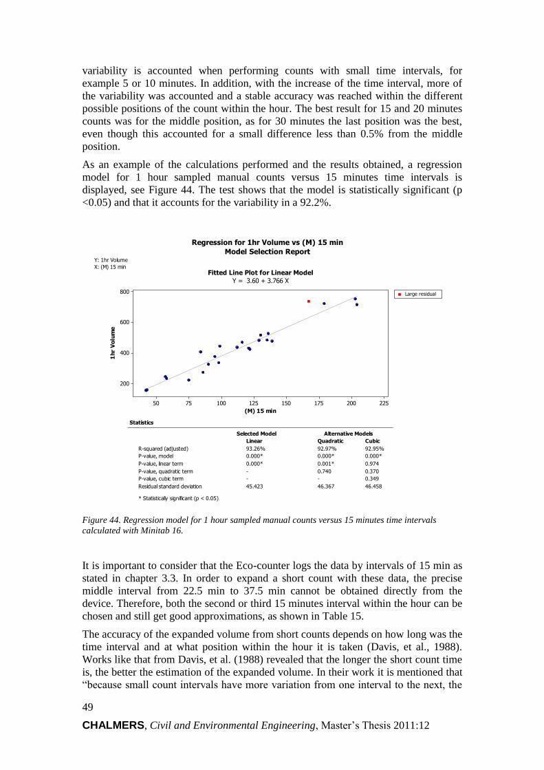
49


variability is accounted when performing counts with small time intervals, for

example 5 or 10 minutes. In addition, with the increase of the time interval, more of

the variability was accounted and a stable accuracy was reached within the different

possible positions of the count within the hour. The best result for 15 and 20 minutes

counts was for the middle position, as for 30 minutes the last position was the best,

even though this accounted for a small difference less than 0.5% from the middle

position.

As an example of the calculations performed and the results obtained, a regression

model for 1 hour sampled manual counts versus 15 minutes time intervals is

displayed, see Figure 44. The test shows that the model is statistically significant (p

<0.05) and that it accounts for the variability in a 92.2%.

Figure 44. Regression model for 1 hour sampled manual counts versus 15 minutes time intervals

calculated with Minitab 16.

It is important to consider that the Eco-counter logs the data by intervals of 15 min as

stated in chapter 3.3. In order to expand a short count with these data, the precise

middle interval from 22.5 min to 37.5 min cannot be obtained directly from the

device. Therefore, both the second or third 15 minutes interval within the hour can be

chosen and still get good approximations, as shown in Table 15.

The accuracy of the expanded volume from short counts depends on how long was the

time interval and at what position within the hour it is taken (Davis, et al., 1988).

Works like that from Davis, et al. (1988) revealed that the longer the short count time

is, the better the estimation of the expanded volume. In their work it is mentioned that

“because small count intervals have more variation from one interval to the next, the

2252001751501251007550

800

600

400

200

(M) 15 min

1h

r V

olu

me

Large residual

Statistics

R-squared (adjusted)

P-value, model

P-value, linear term

P-value, quadratic term

P-value, cubic term

Residual standard deviation

93.26%

0.000*

0.000*

-

-

45.423

Linear

Selected Model

92.97% 92.95%

0.000* 0.000*

0.001* 0.974

0.740 0.370

- 0.349

46.367 46.458

Quadratic Cubic

Alternative Models

Y: 1hr Volume

X: (M) 15 minFitted Line Plot for Linear Model

Y = 3.60 + 3.766 X

* Statistically significant (p < 0.05)

Regression for 1hr Volume vs (M) 15 min

Model Selection Report

50


potential for extracting a non-representative count for the time period being predicted

is high”. Additionally, the middle position is the most favourable within the time to be

expanded. The variability phenomena are illustrated in Figure 45 and Figure 46.

Figure 45. Variability of pedestrian volumes with 5 minutes time intervals; manual count in

Drottninggatan 20-Aug-2010. The mean line serves as a reference to look out the changes in each step.

Figure 46. Variability of pedestrian volumes with 15 minutes time intervals; manual count in

Drottninggatan 20-Aug-2010. The mean line serves as a reference to look out the changes in each step.

0

5

10

15

20

25

30

35

40

45

50

55

12

:00

12

:05

12

:10

12

:15

12

:20

12

:25

12

:30

12

:35

12

:40

12

:45

12

:50

12

:55

13

:00

13

:05

13

:10

13

:15

13

:20

13

:25

13

:30

13

:35

13

:40

13

:45

13

:50

13

:55

Vo

lum

e (

pe

d)

5 min intervals

Pedestrians Variability

Pedestrians Mean volume

0102030405060708090

100110120130

12

:00

12

:15

12

:30

12

:45

13

:00

13

:15

13

:30

13

:45

Vo

lum

e (

pe

d)

15 min intervals

Pedestrians Variability

Pedestrians Mean volume

51


4.6 Example calculation

The following examples illustrate the calculation of the peak hour factor, volume of

design, expansion factors and adjustment factors.

52


53


The daily volume patterns can give the total expected volume for the day when the

coverage count was performed. However, in several weeks, a month or a year the

counted day will have volume variations (high and low volume seasons). For

example, if the counting is performed on a day where an unusual activity was

undergoing, an unexpected or biased result could be obtained unless this could be a

special case and thus the result is right. But, if a general scenario is wanted and what

is expected is an average volume within a time period (e.g. average volume for

Mondays in month “x”), then adjustment factors must be applied, as stated in chapter

2.5.2. This is illustrated below:

54


5 Summary and discussion

Literature review

Part of the theory was obtained from motorized traffic knowledge. This does not mean

that the methodology could not work because volume studies are handled in the same

way independently from where they come from.

Automatic Counters

The Eco-counter was only able to provide the data by direction. Therefore a direct

comparison for individual sidewalks could not be performed. A general error was

found for both sides, without having the possibility of assessing which side had the

major influence on the results.

The Eco-counter counted everything, including cars, motorcycles, bicycles and

pedestrians. This device could be deemed to be accurate since the data from the

volumes of vehicles and “others” could balance the undercount of pedestrians. In this

matter, the automatic counter could be used with certain restrictions and in specific

conditions; for example, when it is not affected by cars or “others”. In addition, to

filter the data it is necessary to have additional devices such as pneumatic tubes,

another type of automatic counters for bicycles or perform manual counts for the

period that is needed to have the data; which in this case is preferable to rely just on

the manual counts.

The raw data from the Eco-counter can give misleading results. If the Eco-counter

data would not have been refined, the error could be much lower giving a first

impression of high accuracy. Furthermore, the data from the pneumatic tubes used to

refine the Eco-counter presented errors itself.

It was found that the resulting volume patterns from the Eco-counter could be biased

by several factors. One factor is that errors from the device were noticed to be

variable within certain range. For this investigation, it is not completely clear if the

error is variable during the whole day or if it could turn to be constant with more

samples. Furthermore, when refining the data, errors from the other devices and

methods were merged to the one of the Eco-counter. These factors, along with the

small intrinsic variation of each street, can result on an unexpected outcome.

There was not enough data (only two weeks per section) to assess properly the Eco-

counter samples. With only two daily samples in every section, the judgment of which

is the real value could be easily biased. It is important that at least 4 samples (1

month) are collected in order to preclude any unusual value that could have been

affected by external factors.

General Statistics

It was noticed that the majority of pedestrians were using the street instead of the

sidewalks with arcades. A possible reason explaining this behaviour is that people

preferred opened environments to walk rather than using a sidewalk that gave the

impression of a big hallway with a far end, as shown in Figure 10. Furthermore, all

the arcades in both streets did not have shops or centre of activities; conversely these

were generally in the narrow sidewalk. Also, it is possible that the people chose a

specific sidewalk (the narrowest one without arcades) because of their destination

(related to origin-destination walking behaviour).

55


Properties, like gender, age and walking direction, are characteristic of the complete

street and thus a classification scheme from any section and any sidewalk can be

adopted. The preceding statement can be an advantage to be used in manual counts

when the classification could be limited in some points due to high volumes (> 700

peds/hr/sidewalk). In this respect, if the street is the same and has the same

characteristics (e.g. same land use, sidewalks at both sides, etc.), the side with the

lower volume could be classified and the results applied to the other. However, one

property that did not represent a problem to classify was the direction, thus being

performed at all times.

The age interval for the adult’s classification can be regarded as wide, from 14-60

years old. This was considered based on the judgement that people within this age

interval have the same walking characteristic and abilities. Additionally, to add more

age intervals would make the manual count more complex for the personnel, putting

at risk the accuracy and reliability of it.

One of the most important factors affecting the volume of pedestrians in the area was

the land use. Drottninggatan and Kyrkogatan are situated in a highly commercial area

and both showed similar properties. Some differences in daily volumes were

appreciated between different sections, perhaps because of the different activities

available in each. Furthermore, the hourly volume proportions for all sections were

close enough to be considered as equal.

Volume patterns

The hourly volume proportions are independent of the total volume. They depend on

how the volume is distributed along the day. Generally, one has to accept some

percentage differences (e.g. ± 2% from intrinsic properties of the streets) in the hourly

volume proportions between locations and days, in order to group their daily volume

patterns. This is illustrated in Table 16 below. When percentage differences are set

according to expert judgment or the proposed use of the data, one will be able or not

to group certain days and locations into a single daily volume pattern.

Table 16. Example of how volume proportions are independent of volumes and how the average fit in

all cases.

Volume Volume Proportions

Time Mon. Tue. Wed. Thu. Fri. Avg. Mon. Tue. Wed. Thu. Fri. Avg.

12:00 67 74 77 54 90 72 19% 19% 18% 20% 17% 18%

13:00 54 59 64 41 77 59 15% 15% 15% 15% 15% 15%

14:00 48 53 58 35 71 53 13% 13% 14% 13% 14% 14%

15:00 45 50 55 32 68 50 13% 13% 13% 12% 13% 13%

16:00 56 62 66 43 79 61 16% 16% 15% 16% 15% 16%

17:00 48 53 58 35 71 53 13% 13% 14% 13% 14% 14%

18:00 39 43 49 26 62 44 11% 11% 11% 10% 12% 11%

Total 357 394 427 266 518 392

56


Even though the data from the manual counts was logged in 5 min intervals, the data

was grouped into 15 minutes to be able to compare it with the automatic counters. The

researchers thought that it might be good to acquire the data the more detailed as

possible to get more knowledge of the different time interval behaviours.

Videos

Due to the limitation of the width recording capacity of the video camera and the

characteristics of the street itself, i.e. parked cars, arcades and columns which

restricted the view; only one sidewalk was considered to compare the count provided

by the video and the manual count (in this case the one with the clearest view).

When performing the manual counts and analyzing the videos, some characteristic

behaviour within the people walking were observed. For example, pedestrians had a

high confidence about their walking priority; they believed that drivers respected their

rights. Also, people tended to walk with variable speed (e.g. different walking

purposes).

Model

The equations used to evaluate the different time intervals for the manual counts are

limited in time and space. General equations will require wide data collection plans, to

account for different land uses and for the main 12 hours of the day.

General

The samples taken were limited due to time restrictions and also the size of the study.

Further studies are always recommended in order to get a good knowledge in this

field. The conclusions were drawn based on this small amount of samples, meaning

that they could be subjected to changes.

It is important to consider the economical aspects of the manual counts versus the

automatic counts. One must think if it is proper to invest in new technologies that

could provide unreliable data or use traditional methods such as the manual counts

that provide data with higher quality.

57


6 Conclusions

Pedestrian volumes and their patterns were generated using the approaches for

counting pedestrians presented here. The methodology needs to be assessed and

improved since this is a pilot study made in two streets in the city of Gothenburg. In

this respect, further studies and tests using this methodology are required with a

broader data collection plan.

It was found that between 10 to 12 hours of the day is the main time for pedestrians’

activities, e.g. ranging from 7:00-19:00. This statement confirms what was found in

previous literatures.

The volume proportions between Drottninggatan and Kyrkogatan seem to couple

according to the land use variable, both for weekdays and weekend days. The location

for both streets considered as a commercial zone, reflect similar behaviour among the

pedestrians. Additionally, it is concluded that a count can be performed anywhere in

the street. The location can be selected based on how suitable the counters can be set.

The flow of people to each direction was independent from the volumes of people that

walked in the area. In this respect, more people headed west to the main avenues such

as Östra Hamngatan and Fredsgatan.

The size and characteristics of the sidewalk were key factors in the influence of

people walking on the street. Narrow sidewalks (1.2-1.5 meters) without arcades

accounted for most of the volume and people tended to walk on the street beside it. In

the other hand, sidewalks with arcades (2-3 meters) attracted less pedestrians.

Manual counts are an accurate source for collecting data if performed with proper

procedures and if the personal is committed to perform the task. A disadvantage of

this approach is that they require man-hours which implies that this type of count

cannot be performed for a continuous period of time such as the automatic counts.

At the beginning of each coverage count the personnel felt unfamiliar, not completely

focused or used to the procedure. After the first 5 minutes it was comfortable enough

to proceed properly since the personnel became more active and focused during the

counting time. Also, detailed manual counts can become tedious for certain volumes.

On average it was found that flows higher than 700 pedestrians/hr/sidewalk are

complicated to classify.

The automatic count technology for pedestrians used in this study is good for

generating patterns since it develops continuous counts, which allows collecting large

amount of samples and generates more stable statistical data. However, in order to get

good approximations of the patterns, the Eco-counter must be located in

controlled/regulated environment. Moreover, the data filtering is hard to perform

especially when the data requires to be refined by using other counters like pneumatic

tubes. These technologies presented a high percentage of error.

Video counts are time-consuming when it comes to analyse them, but they provide

highly accurate data since it can be examined in a repetitive manner. Mainly, the

videos showed that the errors from the automatic counters are due to external factors.

Errors from the Eco-counter are not affected by the volume of pedestrians. Instead,

they were due to other factors like the density of pedestrian walking through the

counter, where people walking in groups were omitted. Another aspect was the

58


objects that could block the counter for certain times of the day, e.g. a car, a bicycle, a

person, etc.

The Eco-counter should not be located near stores or bus stop or any kind of source of

pedestrians or where pedestrians can gather. This causes the counts to have a bias,

reflected by successive peaks.

In general, it was found that pneumatic tubes are unstable and unreliable in urban

areas due to cars driving at low speed and because of people altering the device

(generally by curiosity). Consequently the data from it had errors that added to the

errors from the Eco-counter when filtering the data, thus deviating the final result.

Regression models were used to determine an efficient short count interval in order to

save money and resources when performing a manual count sampling. The models

provided a good estimate of the volumes for the hour that could be used to reduce the

amount of man-hours. In this matter, the manual counts should be performed at least

for 15 minutes and for the middle position (e.g. 20–35, 25-40 min) within the hour

being counted. The bigger the time interval counted, the closer to the reality are the

results from the model.

59


7 Recommendations

It is recommended that when performing pedestrian counts, different approaches are

considered at the same time. The automatic counters are good to use for obtaining

long term data, but always together with an additional counting method like the

manual counting. The latter helps to corroborate that the data is reliable/accurate and

provides facts that can be used to calibrate/correct any error in the automatic devices.

The methodology consists on counting pedestrians using the tally sheet presented in

this study, and to compare the data obtained with this approach with the one obtained

with automatic and video counting technologies. As a recommendation, the short

counts should be performed for at least 15 minutes and logged in 5 minutes intervals

(the latter necessary if a detailed analysis of the data is required).

Manual counts are recommended to be performed in small studies that do not require

long term data collection. Pre-training of the personnel is highly recommended for

obtaining accurate and reliable manual counts data. If automatic counters are going to

be used, it is always good to test their performance, for example, comparing them

with manual counts or video counts.

Try different approaches when setting up the Eco-counter device. For example, a

good approach could be to put the device in a 45 degrees angle to avoid the

undercounting.

7.1 Future Research

Perform surveys of non-motorized users, including Origin/Destination.

Perform counts in intersections, putting emphasis on accounting for the change

of walking direction between streets.

Try new counting technologies, like video processing.

Localization of counters in the public transportation.

Create simulations of macro scenarios of the city. For example, using Vissim

with the volumes and patterns obtained, to develop macro models of the

volumes of people walking in the city.

Count for long time periods to obtain monthly and seasonal variations.

60


REFERENCES

Alta Planning & Design, 2010. National Bicycle and Pedestrian

Documentation Project (NBPD): Instruction manual. [Online] Available at:

http://bikepeddocumentation.org/ [Accessed 29 July 2010].

Aultman-Hall, L., Lane, D., Lambert, Rebecca R., 2009. Assessing the Impact

of Weather and Season on Pedestrian Traffic Volumes. [Internet] University of

Vermont: Transportation Research Board (TRB). Available at:

http://www.uvm.edu/~transctr/?Page=pubs_journals.html&SM=_pubsmenu.ht

ml [Accessed 22 July 2010]

Bladh, A., Andersson, B-M., Johnson, Bo., Collins, B. Rågdell, K., Schoster,

G. 1984. Gångtrafikundersökning i city. Göteborg, Sverige.

Stadsbyggnadkontoret. Trafikplaneavdelningen, Publikation 1984:12.

Trafikdata 8/84.

Davis, S.E., King, L. E., & Robertson, H. D., 1988. Predicting Pedestrian

Crosswalk Volumes. Driver Performance, Pedestrian Planning, and Bicycle

Facilities. Transportation Research Record, 1168, pp. 25-30.

Diogenes, Mara C., Greene-Roesel, R., Arnold, Lindsay S., Ragland, David

R., 2006. Pedestrian Counting Methods at Intersections: a Comparative Study

(Revised). [PDF] August 2006 ed. California-Berkeley. Available at:

http://escholarship.org/uc/item/208349wf

Eco-counter, 2010. Pyroelektrisk sensor. [Online] (Updated date NA).

Available at: http://www.eco-compteur.com/ Tracking: Solutions/Sensorer för

gåntrafik/pyroelektrisk sensor.

[Accessed: 2010-12-21]

Eniro, 2011. Göteborgs kartan. [Online] Available at:

http://kartor.eniro.se/m/IUj5E

[Accessed: 15 January 2011]

FHWA - Federal Highway Administration, 2001. Traffic Monitoring Guide.

[Internet] United States: FHWA. Available at:

http://www.fhwa.dot.gov/ohim/tmguide/ [Accessed 22 July 2010].

Fransson, Erik, 2009. Utvärdering - detekteringsutrustning: Eco-counter

Detektering av cykel- och gångtrafikanter. Stockholm, Sweden: Vectura

Consulting AB.

http://bikepeddocumentation.org/

http://www.uvm.edu/~transctr/?Page=pubs_journals.html&SM=_pubsmenu.html

http://www.uvm.edu/~transctr/?Page=pubs_journals.html&SM=_pubsmenu.html

http://escholarship.org/uc/item/208349wf

http://www.eco-compteur.com/?wpid=14879&_lg=sv_SE

http://kartor.eniro.se/m/IUj5E

http://www.fhwa.dot.gov/ohim/tmguide/

61


Garber, Nicholas J., Hoel, Lester A., 2002. Traffic and Highway Engineering.

Third Edition. University of Virgina: Brooks/Cole Thomson Learning.

Greene-Roesel, R., Diogenes, Mara C., Ragland, David R., Lindau, Antonio

L., 2008. Effectiveness of a Commercially Available Automated Pedestrian

Counting Device in Urban Environments: Comparison with Manual Counts

(Revised). [PDF] July 2007 ed. California-Berkeley. Available at:

http://safetrec.berkeley.edu/news/08-0503session240ryanposter.pdf

Jonsson, Thomas, 2005. Predictive models for accidents on urban links – A

focus on vurnerable road users. [Internet] Ph. D. Sweden: Lund University.

Available at: http://www.lu.se/o.o.i.s?id=12683&postid=24269 [Accessed 20

June 2010]

Minitab, 2010. Minitab help file. [Internet] United States: Minitab. (Select

English) Available at: http://www.minitab.com/en-

US/products/minitab/documentation.aspx?msw=1&langType=1033

[Accessed: 17 January 2011]

Niska, et al. 2010. Metoder för skattning av gång -och cykeltrafik:

Kartläggning och kvalitetsbedömning. Linköping, Sverige. VTI rapport 686.

Ragland, David R., Jones, Michael G., 2010. Seamless Travel: Measuring

Bicycle and Pedestrian Activity in San Diego County and its Relationship to

Land Use, Transportation, Safety, and Facility Type. [Internet] California:

SafeTREC and Alta Planning+Design. Available at:

http://www.altaplanning.com/caltrans+seamless+study.aspx [Accessed 2010-

07-22]

Robertson, H. Douglas, Hummer, Joseph E., Nelson, Donna C., 1994. Manual

of Transportation Engineering Studies. Englewood Cliffs, NJ: Prentice Hall

and the Institute of Transportation Engineers (ITE).

Roess, Roger P., Prassas, Elena S., McShane, William R., 2004. Traffic

Engineering. Third Edition. Upper Saddle River, NJ: Pearson Prentice Hall.

Sauter, D., 2010. Measuring walking: Towards internationally standardized

monitoring methods of walking and public space. [Online] Available at:

http://www.measuring-walking.org/ [Accessed: 27 September 2010]

Schneider, R., Arnold L., Ragland D., 2008. A Methodology for Counting

Pedestrians at intersections: Using Automated Counters to Extrapolate Weekly

http://safetrec.berkeley.edu/news/08-0503session240ryanposter.pdf

http://www.lu.se/o.o.i.s?id=12683&postid=24269

http://www.minitab.com/en-US/products/minitab/documentation.aspx?msw=1&langType=1033

http://www.minitab.com/en-US/products/minitab/documentation.aspx?msw=1&langType=1033

http://www.altaplanning.com/caltrans+seamless+study.aspx

http://www.measuring-walking.org/

62


Volumes from Short Manual Counts (Revised). [PDF] November 2008 ed.

California-Berkeley. Available at:

http://www.tsc.berkeley.edu/news/TSCtrb2009/SchneiderCountingPeds09-

3172.pdf

Schneider, R., Patton, R., Toole, J., Raborn, C., 2005. Pedestrian and Bicycle

Data Collection in United States Communities: Quantifying Use, Surveying

Users, and Documenting Facility Extent. [PDF] January 2005. Available at:

http://www.walkinginfo.org/library/details.cfm?id=2065

Turvey, I.G., May, A.D., Hopkinson, P.G., 1987. Counting Methods and

Sampling Strategies Determining Pedestrian Numbers [Online]. Institute of

Transport Studies, University of Leeds. Working Paper 242. Available at:

http://eprints.whiterose.ac.uk/2316/ [Accessed 3rd July 2010].

Urban Audit, 2004. Database for the city of Gothenburg and Stockholm.

(Hitting Data that can be accessed) [Online] Available at:

http://www.urbanaudit.org/DataAccessed.aspx [Accessed: 30 January 2011]

http://www.tsc.berkeley.edu/news/TSCtrb2009/SchneiderCountingPeds09-3172.pdf

http://www.tsc.berkeley.edu/news/TSCtrb2009/SchneiderCountingPeds09-3172.pdf

http://www.walkinginfo.org/library/details.cfm?id=2065

http://eprints.whiterose.ac.uk/2316/

http://www.urbanaudit.org/DataAccessed.aspx

63


APPENDIX 1 – Volume proportions for each day and

section

Figure 47. Section 1 in Drottninggatan.

Figure 48. Section 2 in Drottninggatan.

0,0%

2,0%

4,0%

6,0%

8,0%

10,0%

12,0%

14,0%

00

:00

01

:00

02

:00

03

:00

04

:00

05

:00

06

:00

07

:00

08

:00

09

:00

10

:00

11

:00

12

:00

13

:00

14

:00

15

:00

16

:00

17

:00

18

:00

19

:00

20

:00

21

:00

22

:00

23

:00

Pro

po

rtio

ns

(hr/

24

hr)

Section 1


0,0%

2,0%

4,0%

6,0%

8,0%

10,0%

12,0%

14,0%

16,0%

18,0%

00

:00

01

:00

02

:00

03

:00

04

:00

05

:00

06

:00

07

:00

08

:00

09

:00

10

:00

11

:00

12

:00

13

:00

14

:00

15

:00

16

:00

17

:00

18

:00

19

:00

20

:00

21

:00

22

:00

23

:00

Pro

po

rtio

ns

(hr/

24

hr)

Section 2


64


Figure 49. Section 3 in Kyrkogatan.

Figure 50. Section 4 in Kyrkogatan.

0,0%

2,0%

4,0%

6,0%

8,0%

10,0%

12,0%

14,0%

16,0%

18,0%

00

:00

01

:00

02

:00

03

:00

04

:00

05

:00

06

:00

07

:00

08

:00

09

:00

10

:00

11

:00

12

:00

13

:00

14

:00

15

:00

16

:00

17

:00

18

:00

19

:00

20

:00

21

:00

22

:00

23

:00

Pro

po

rtio

ns

(hr/

24

hr)

Section 3


0,0%

2,0%

4,0%

6,0%

8,0%

10,0%

12,0%

14,0%

00

:00

01

:00

02

:00

03

:00

04

:00

05

:00

06

:00

07

:00

08

:00

09

:00

10

:00

11

:00

12

:00

13

:00

14

:00

15

:00

16

:00

17

:00

18

:00

19

:00

20

:00

21

:00

22

:00

23

:00

Pro

po

rtio

ns

(hr/

24

hr)

Section 4


65


Appendix 2 – Volumes obtained with the manual

counts

Notes:

On the italicized red dates, the volumes were not classified for side A.

Cars are counted for the street independently of each side.

Sections and Dates 12 PM

Car Female Male Other

Drottninggatan-Östra H/Freds

2010-08-20

A 154 102 24

B 96 79 0

2010-08-27

A 139 146 11

B 100 98 97 0

Drottninggatan-Freds/Östra L

2010-09-02

A 66 426 24

B 151 137 0

2010-09-06

A 64 455 16

B 143 155 1

2010-09-07

A 83 454 25

B 139 143 0

2010-09-13

A 75 489 27

B 106 126 1

Kyrkogatan-Freds/Östra L

2010-09-20

A 55 69 1

B 66 87 62 6

2010-09-22

A 80 65 13

B 60 32 56 0

Kyrkogatan-Östra H/Freds

2010-09-29

A 67 164 188 11

B 93 80 0

2010-10-04

A 62 132 102 11

B 98 90 0

66


2010-10-08

A 59 118 132 14

B 104 89 0



Drottninggatan-Ostra H/Freds

2010-08-20

A 116 93 27

B 99 98 0

2010-08-27

A 113 157 16

B 85 105 93 0

Kyrkogatan-Ostra H/Freds

2010-10-02

A 65 260 192 8

B 120 110 0




2010-10-02

A 57 336 241 15

B 160 113 0




2010-08-26

A 118 67 31

B 50 82 59 1

Drottninggatan-Freds/Ostra L

2010-09-06

A 70 329 34

B 79 67 1

2010-09-07

A 58 315 41

67


B 120 80 0


2010-09-27

A 44 153 102 31

B 99 81 1

2010-10-05

A 51 124 86 16

B 82 83 0

Sections and Dates

5 PM



2010-08-24

A 43 42 29

B 61 76 1

2010-08-26

A 120 92 41

B 73 71 53 1

Drottninggatan-Freds/Ostra L

2010-09-02

A 56 266 35

B 91 76 0

Kyrkogatan-Freds/Ostra L

2010-09-14

A 38 34 1

B 63 52 30 17

2010-09-23

A 105 54 18

B 67 66 21 1




2010-08-24

A

39 40 16

B

40 37 0

68


APPENDIX 3 – Site setup

Documents

Pedestrian Volume Studies - Chalmers Publication …publications.lib.chalmers.se/records/fulltext/141801.pdfresearch could be performed in subjects such as origin-destination surveys,