CFDSimulationoftheVolvoCarsSlottedWalls Wind …publications.lib.chalmers.se/records/fulltext/143242.pdfCFDSimulationoftheVolvoCarsSlottedWalls Wind Tunnel Master’sThesisinSolidandFluidMechanics

CFD Simulation of the Volvo Cars SlottedWallsWind Tunnel

Master’s Thesis in Solid and Fluid Mechanics

MATTIAS OLANDER

Department of Applied MechanicsDivision of Division of Vehicle Engineering and Autonomous SystemsCHALMERS UNIVERSITY OF TECHNOLOGYGoteborg, Sweden 2011Master’s Thesis 2011:33

MASTER’S THESIS 2011:33

CFD Simulation of the Volvo Cars Slotted Walls Wind Tunnel

Master’s Thesis in Solid and Fluid MechanicsMATTIAS OLANDER

Department of Applied MechanicsDivision of Division of Vehicle Engineering and Autonomous Systems

CHALMERS UNIVERSITY OF TECHNOLOGY

Goteborg, Sweden 2011

CFD Simulation of the Volvo Cars Slotted Walls Wind TunnelMATTIAS OLANDER

c©MATTIAS OLANDER, 2011

Master’s Thesis 2011:33ISSN 1652-8557Department of Applied MechanicsDivision of Division of Vehicle Engineering and Autonomous SystemsChalmers University of TechnologySE-412 96 GoteborgSwedenTelephone: + 46 (0)31-772 1000

Cover:Velocity streamlines around the S80 inside the PVT tunnel

Chalmers ReproserviceGoteborg, Sweden 2011

CFD Simulation of the Volvo Cars Slotted Walls Wind TunnelMaster’s Thesis in Solid and Fluid MechanicsMATTIAS OLANDERDepartment of Applied MechanicsDivision of Division of Vehicle Engineering and Autonomous SystemsChalmers University of Technology

Abstract

When CFD simulations are performed at Volvo Cars, a case which resemblesthe condition for a car traveling on a open road is simulated. The results fromthese simulations have often proved to be different compared to the results from theexperiments in the Volvo Cars slotted walls wind tunnel. To investigate the reasonbehind these differences a number of CFD simulations of the Volvo Cars wind tunnelhave been performed. The simulations have been focused on three main cases, emptytunnel, tunnel with a simplified S60 and tunnel with a detailed S80. The resultshave been compared to ordinary CFD simulations and to newly made experimentsin the wind tunnel. The flow produced by the numerical simulations in the emptywind tunnel has proved to be largely asymmetric due to the asymmetric geometryof the slotted walls’ support structure. This has greatly affected the flow around acar in the tunnel resulting in a different flow field compared to the standard CFDsimulation. The drag and lift coefficient of the S60 and S80 have been lower in theCFD simulations of the wind tunnel compared to the ordinary CFD simulations,which is the opposite to what have been found when comparing the standard CFDsimulations to the real experiments in the tunnel. The reason behind this is believedto be mainly due to the geometry simplifications of the simulated tunnel and theuniform inlet boundary condition, which have resulted in a very much more uniformflow in the CFD simulations compared to the experiments.

Keywords: CFD, Wind Tunnel, Slotted Walls, Mesh, Wind loads, Aerodynamics, VolvoCars, Experiment

, Applied Mechanics, Master’s Thesis 2011:33 I

II , Applied Mechanics, Master’s Thesis 2011:33

Contents

Abstract I

Contents III

Preface V

List of Abbreviations VI

1 Introduction 11.1 Background . . . . . . . . . . . . . . . . . . . . . . . . . . . . . . . . . . . 11.2 Purpose . . . . . . . . . . . . . . . . . . . . . . . . . . . . . . . . . . . . . 11.3 Goal . . . . . . . . . . . . . . . . . . . . . . . . . . . . . . . . . . . . . . . 11.4 Limitations . . . . . . . . . . . . . . . . . . . . . . . . . . . . . . . . . . . 11.5 Method . . . . . . . . . . . . . . . . . . . . . . . . . . . . . . . . . . . . . 1

2 Background 32.1 The Volvo Cars Slotted Walls Wind Tunnel - PVT . . . . . . . . . . . . . 32.2 The Standard CFD Procedure at Volvo Cars . . . . . . . . . . . . . . . . . 5

3 Theory 73.1 The Governing Equations . . . . . . . . . . . . . . . . . . . . . . . . . . . 73.2 The Near Wall Flow . . . . . . . . . . . . . . . . . . . . . . . . . . . . . . 7

4 Method 94.1 Geometry . . . . . . . . . . . . . . . . . . . . . . . . . . . . . . . . . . . . 9

4.1.1 PVT Tunnel . . . . . . . . . . . . . . . . . . . . . . . . . . . . . . . 94.1.2 S60 . . . . . . . . . . . . . . . . . . . . . . . . . . . . . . . . . . . . 114.1.3 S80 Closed Front . . . . . . . . . . . . . . . . . . . . . . . . . . . . 124.1.4 S80 Open Cooling . . . . . . . . . . . . . . . . . . . . . . . . . . . . 13

4.2 Mesh . . . . . . . . . . . . . . . . . . . . . . . . . . . . . . . . . . . . . . . 144.2.1 PVT Tunnel . . . . . . . . . . . . . . . . . . . . . . . . . . . . . . . 144.2.2 S60 . . . . . . . . . . . . . . . . . . . . . . . . . . . . . . . . . . . . 154.2.3 S80 Closed Front . . . . . . . . . . . . . . . . . . . . . . . . . . . . 164.2.4 S80 Open Cooling . . . . . . . . . . . . . . . . . . . . . . . . . . . . 17

4.3 Calculation Settings . . . . . . . . . . . . . . . . . . . . . . . . . . . . . . 184.3.1 Empty Tunnel . . . . . . . . . . . . . . . . . . . . . . . . . . . . . . 214.3.2 Tunnel With Simple S60 . . . . . . . . . . . . . . . . . . . . . . . . 214.3.3 Tunnel With S80 Closed Front . . . . . . . . . . . . . . . . . . . . . 224.3.4 Tunnel With S80 Open Cooling . . . . . . . . . . . . . . . . . . . . 22

4.4 Postprocessing . . . . . . . . . . . . . . . . . . . . . . . . . . . . . . . . . . 22

5 Results and Discussion 245.1 Empty Tunnel . . . . . . . . . . . . . . . . . . . . . . . . . . . . . . . . . . 24

5.1.1 Asymmetrical Behaviour . . . . . . . . . . . . . . . . . . . . . . . . 245.1.2 Axial pressure gradient . . . . . . . . . . . . . . . . . . . . . . . . . 265.1.3 Nozzle Contraction . . . . . . . . . . . . . . . . . . . . . . . . . . . 265.1.4 Comparison With Experiments . . . . . . . . . . . . . . . . . . . . 28

5.2 Tunnel With Simplified S60 . . . . . . . . . . . . . . . . . . . . . . . . . . 335.2.1 Asymmetrical Behaviour . . . . . . . . . . . . . . . . . . . . . . . . 335.2.2 PVT Tunnel impact on pressure coefficients . . . . . . . . . . . . . 37

, Applied Mechanics, Master’s Thesis 2011:33 III

5.3 Tunnel With S80 Closed Front . . . . . . . . . . . . . . . . . . . . . . . . . 395.3.1 Asymmetrical Behaviour . . . . . . . . . . . . . . . . . . . . . . . . 395.3.2 PVT Tunnel impact on pressure coefficients . . . . . . . . . . . . . 425.3.3 Comparison With Experiments . . . . . . . . . . . . . . . . . . . . 48

5.4 Tunnel With S80 Open Cooling . . . . . . . . . . . . . . . . . . . . . . . . 495.4.1 PVT Tunnel impact on pressure coefficients . . . . . . . . . . . . . 495.4.2 Comparison With Experiments . . . . . . . . . . . . . . . . . . . . 49

6 Conclusions 51

7 Recommendations and Future Work 52

References 53

IV , Applied Mechanics, Master’s Thesis 2011:33

Preface

This master thesis has been performed at the Group at Volvo Cars in collaboration with theDepartment of Applied Mechanics, Chalmers University of Technology, Sweden, during thespring of 2011. Mattias Olander has been the student performing the master thesis withSimone Sebben as supervisor at Volvo Cars and Lennart Lofdahl as examiner at Chalmers.

Acknowledgement

I want to thank my supervisor at Volvo Cars, Simone Sebben, for her support and helpwith the CFD process during this master thesis. Without her this project would not havebeen possible to be realized. I want to thank Tim Walker for all the valuable discussionswe have shared which have helped me tremendously. I also want to thank my examiner,Lennart Lofdahl for always being available whenever I had any questions regarding theproject.

I want to thank thesis worker Erik Lindmark for assisting me when various geometrieshad to be created, for providing me with tips and trix about the softwares used in thisproject and for the discussions we had. I want to thank CFD engineer Patrick Sondell whosehelp regarding softwares and other computer related issues have been deeply appreciated.I want to say thanks to CFD engineer Mattias Hejdesten for answering all my questionswhen Simone was not available. I also want to thank PhD student Lennart Sterken forenlighten me about micro drag and especially for picking me up at the airport, a big thanks!

Last I want to say thank you to the personnel at the PVT tunnel for lending me theirtime and energy and all the employees at the Volvo Cars aerodynamic department for thegreat atmosphere that I have experience during my time at Volvo Cars.

Goteborg June 2011Mattias Olander

, Applied Mechanics, Master’s Thesis 2011:33 V

List of Abbreviations

CFD Computational Fluid DynamicsCAD Computer Aided DesignPVT Volvo Cars Slotted Walls Wind TunnelQUICK Quadratic Upstream Interpolation for Convective KineticsBLCS Boundary Layer Control SystemGESS Ground Effect Simulation SystemWDU Weel Drive UnitsPID Property IDAiolos Company which upgraded and calibrated the wind tunnel

VI , Applied Mechanics, Master’s Thesis 2011:33

1 Introduction

1.1 Background

Today the exterior aerodynamic CFD simulations at Volvo Cars are performed with avirtual domain around the car, which has boundary conditions that resembles open roadconditions, hence very different from the conditions of the Volvo Cars’ slotted walls windtunnel. In addition to that, the complete ground is set as moving in the CFD simulationswhich is a lot different from the advanced boundary layer control system and 5-belt movingground system used in the wind tunnel. It is therefore complicated to compare the CFDresults with the results from the wind tunnel as the two cases are very different from eachother. Also, after the wind tunnel was upgraded in 2007, no extensive CFD simulation hasbeen made on the wind tunnel, thus there exist no validity check of the CFD results.

1.2 Purpose

The purpose of this master thesis is to carry out extensive CFD simulations of the windtunnel and to compare the results with results from both standard CFD simulations andreal experiments in the wind tunnel, with the aim to be able to either verify the standardCFD simulations or explain the differences. The reasons behind certain results from thewind tunnel will be investigated and explained. The aim is also to get a better under-standing of the flow field in the wind tunnel and to get a better picture of how the slottedwalls affects the flow, especially with a car inside the tunnel.

1.3 Goal

The main goal of this master thesis understand the differences in flow field and forcesbetween the standard CFD simulation and the wind tunnel results.

1.4 Limitations

The mesh will be limited to a maximum of approximate 100 million cells and the 3D-modelof the wind tunnel is simplified to only include objects that are at least approximately 100mm large, which means that small objects like for example cables are not modeled. Thewind tunnel is only modeled from the start of the nozzle and to the end of the diffuser,hence the complete closed air-path that includes the bends and the main fan is not partof the model. The simulations will only be performed with the same main settings whichis used in the standard procedure at Volvo Cars. This mean that, for example, only therealizable k-epsilon turbulence model will be used and no other turbulence model will betested. In addition, all computations were performed in steady-state.

1.5 Method

The program ANSA will be used to clean up the CAD of the wind tunnel and prepare it formeshing. Before starting the meshing procedure the CAD is going to be compared to thereal wind tunnel and if anything important is missing it will be added manually in ANSA.Harpoon will be used as mesher and Fluent to perform the calculations. The results will beexported to Ensight for analysis and visualization. The first simulations will be performedon one half of the tunnel, with the boundary layer control system and the moving groundsystem turned of, just to ensure that the mesh is of good quality. The boundary layercontrol system will then be turned on step wise to make sure that the conservation of mass

, Applied Mechanics, Master’s Thesis 2011:33 1

through the domain is always satisfied. When successful simulations have been performedwith the boundary control system in place, then the complete tunnel will be simulated andcompared to the simulations performed on one half on the tunnel to distinguish if the flowis symmetrical. When the empty tunnel simulations are completed, a simple geometry ofa S60 will be implemented in order to quickly investigate the complexity of simulationsinvolving a car in the tunnel. The last step is then to put in a real car model of a S80which will be possible to compare with the experiments.

2 , Applied Mechanics, Master’s Thesis 2011:33

2 Background

2.1 The Volvo Cars Slotted Walls Wind Tunnel - PVT

The construction of the Volvo Cars wind tunnel was completed in the mid 1980s and it wasfully operational in 1986. It featured a horizontally closed air-path with a 6.6 m wide and4.1 m high test section of slotted walls and ceiling, where the longitudinal slots created a30% open-area ratio with the purpose of minimizing the blockage effects of the walls. Thetunnel’s closed air-path can be seen in Figure 2.1 which also shows parts of the slottedceiling in the test section.

Figure 2.1: The Volvo Cars slotted walls wind tunnel

In 2006 the wind tunnel was upgraded to the specifications which it still has today in2011. The upgrade included a complete moving ground system and a new boundary layercontrol system (BLCS). The fan power was increased from 2.3 MW to 5 MW to provide awind speed of 250km/h in the test section.

The 5-belt moving ground system consist of a center belt and four wheel drive units(WDU) that can be moved to different positions depending on the vehicle’s track width.The WDUs can be configured with three different belt widths, 280 mm, 360 mm and 410mm and if necessary placed asymmetrically around the center belt.


Figure 2.2: The layout of the floor

The BLCS consist of a boundary layer scoop situated just before the test section (basicscoop), floor mounted suction in front of the turn table in two steps(1st and 2nd suction)and tangential blowing behind the WDUs and the center belt. The air removed by thebasic scoop is inserted above the slotted ceiling in the direction of the flow by two ductslocated at the front wall of the test section. The air removed by the 1st and 2nd suction ispartially used for the tangential blowing while the rest is inserted on the right and left sideof the front wall, behind the slotted walls. A schematically drawing of the moving groundsystem and boundary control system is showed in Figure 2.2.

The tunnel have three different configurations; Scoop only, Ground effects simulationsystem(GESS) off and Aerodynamic mode. For the Scoop only mode, only the basic scoopis operating with everything else turned off. In GESS off also the 1st and 2nd suction isturned on. For the Aerodynamic mode everything is activated.

The wind tunnel test section is not completely symmetric as four additional verticalsupport beams together with two horizontal beams are situated at the right side where thecontrol room is housing. This is due to the slotted walls on the control room side havingwindows made of glass in order the make it possible to see through them. The additionalsupport beams can be seen to the left in Figure 2.3, which shows the inside of the testsection and the scale under the tunnel floor.


Figure 2.3: The slotted walls and the scale situated under the tunnel floor

For any further information regarding the upgrade of the PVT tunnel, see Ref. [1].

2.2 The Standard CFD Procedure at Volvo Cars

When CFD simulations are performed at Volvo Cars open road conditions are intendedto be simulated. This is done by creating a large rectangular box around the car modelrepresenting the domain, which can be seen in Figure 2.4, and then applying symmetrywall conditions to the roof and side walls. A uniform velocity distribution is applied to theinlet and a zero pressure condition at the outlet.

Figure 2.4: The domain used when performing standard CFD simulations

To simulate the car traveling along a road, the wheels are rotated and the completeground is set as a moving ground boundary condition. To model the rotating wheel ac-curately is a difficult process in CFD and there exist different approaches. At Volvo CarsMRF zones are used which means that the fluid situated inside in between the rim spokes


are rotated along with the wall surfaces of the rims and tires which are not normal to theflow.

As the aerodynamic simulations at Volvo Cars are performed with moving groundand rotating wheels, care has to be taken concerning the tires deformation. In realitywhen a car is stationary the tires are deformed by the vehicle’s own weight. When thewheels are rotating the centrifugal force acts on the tires and the tires experiences threedifferent deformations in addition to the deformation caused by the car’s weight. The threedeformations are; radial expansion, axial contraction and vertical displacement.

To represent the deformation of the tires, a procedure at Volvo Cars is performed calledmorphing, which means that the surface mesh of the tires are deformed. The morphingprocedure was created in a master thesis project performed by Peter Mlinaric [2] wherealso the use of MRF zones for modelling rotating wheel was studied.


3 Theory

In this chapter the theory behind the numerical simulations performed in this master thesisis briefly stated and explained. For more detailed information the reader is directed to theFluent Theory Guide and to Ref. [4].

3.1 The Governing Equations

The flow of a Newtonian fluid is described by the governing equations consisting of thecontinuity equation and the Navier Stokes equations. For automotive industry calculationsthe velocity of the flow is never any higher than 250 km/h and therefore the flow canbe considered to be incompressible. The incompressible continuity and Navier Stokesequations is displayed below by equation 3.1 and equation 3.2.

∂υi∂xi

= 0 (3.1)

ρ∂υi∂t

+ ρ∂υi∂υj∂xj

= − ∂p

∂xi

+ μ∂2υi

∂xj∂xj

(3.2)

To solve the equations, a solver uses different numerical schemes. In Fluent severaldifferent numerical schemes are available, such as 1st-order upwind, 2nd-order upwind andQUICK with the last two being the most accurate but also less stable. There is alsodifferent interpolation schemes available for the pressure and at Volvo Cars the defaultstandard pressure interpolation scheme is used. The standard scheme uses equation 3.3where the pressure is interpolated at the faces using momentum equation coefficients.

Pf =

Pc0

ap,c0+

Pc1

ap,c11

ap,c0+ 1

ap,c1

(3.3)

3.2 The Near Wall Flow

A turbulent flow is greatly affected by the walls as they are the main source of meanvorticity and turbulence. It is near the walls where the gradients are large and thus wherethe momentum is most affected. It is therefore of high importance in numerical simulationsto accurately predict the near-wall flow.

A turbulent boundary layer consist of different layers with different characteristics.Immediately near the wall there is a very thin viscous sub-layer, followed by the bufferlayer and then the log-law layer. To be able to resolve a complete turbulent boundarylayer and account for the viscous force in the viscous sub-layer, a very fine mesh would beneeded. Since this is not feasible with today’s computer capacity, wall functions are insteademployed to represent the effect of the wall. Normally wall function are used dependingof the value of the variable y+, shown in equation 3.4. y+ is the dimensionless distance tothe wall for the cell closest to the wall and generally the wall functions are valid when y+

is between 30 and 500, the range of the log-law layer.

y+ =ρuTy

μ(3.4)


In Fluent however, a different variable, y∗, is used instead of y+. y∗ is displayed inequation 3.5 and is approximately equal to y+ in equilibrium turbulent boundary layers.Fluent employs the standard wall function when y∗ > 11.225. If y∗ < 11.225 the flow isconsidered to be laminar and a laminar stress-strain relationship is employed. This meansthat it is very important to keep y∗ above 11.225 in areas where high turbulence andvelocity is expected. The ideal would be to have y∗ close to but above 30 in such areas.

y∗ =ρC

(μ1/4)k(1/2)y

μ(3.5)


4 Method

This section describes the process performed in this master thesis in order to obtain theforthcoming results. There were three different main cases simulated, namely; Empty PVTtunnel, PVT tunnel with a simplified S60 and PVT tunnel with a detailed S80. The S80was performed with two different configurations, closed front where only the external flowis simulated and open cooling where also the flow through the engine bay and coolingpackage is included. To be able to compare the results of the PVT tunnel simulations withthe standard procedure at Volvo Cars, simulations according to computational proceduresAEDCAE01 [5] and AEDCAE02 [6] were performed with the S60 and S80 model. Thestandard simulation is referred to as CFD tunnel and the PVT simulation as PVT tunnelthrough out this report.

4.1 Geometry

4.1.1 PVT Tunnel

To be able to keep the amount of cells within a reasonable level and due to the limitedCAD available, only the nozzle, test section and diffuser of the wind tunnel were modeled.This means that some of the characteristics of the wind tunnel were lost, as the effect ofthe 90 degree turns before and after the test section on the flow field was not accountedfor. Also, to ensure to get a stable solution, the domain was extended in the x-directionin three 10 meters long rectangular boxes. The idea was to remove these extensions oneby one to see if their absence affected the solution negatively but since they only slightlyincreased the cell count they were never removed. The outer surface of the wind tunnelcan be seen in Figure 4.1, the yellow part being the extension.

Figure 4.1: The outer domain of the wind tunnel

Figure 4.2 and Figure 4.3 shows a zoom in on the slotted walls with the test section’souter walls and roof removed, for the left and right side respectively. Notice the differencein the support structure of the slotted walls, left side compared to right side.


Figure 4.2: The domain of the test section with the test section’s outer walls removed, leftside

Figure 4.3: The domain of the test section with the test section’s outer walls removed,right side

The domain was restricted by the available CAD geometry of the wind tunnel whichonly included the nozzle, diffuser and the main parts of the test section. Objects likecable ladders and air hoses were not part of this CAD and therefore not included. TheCAD was also simplified, meaning that objects smaller than approximately 10 cm wereremoved. The biggest objects missing in the CAD was two overhead cranes, one situatedabove the slotted ceiling and the other one at the end of the diffuser. The first one wasnot believed to affect the flow significantly because of its position away from the free flowand rather small size and was therefore left out. The other crane’s influence however couldnot be minimized that easily as its position was in the free flow, even tough far from thetest section. It was decided to proceed with the calculation without the cranes but if theresults showed difference between the CFD and experiments which could be because of theabsence of the cranes they would be created by hand and added to new simulations.


Figure 4.4: The geometry of the floor

The floor of the test section, which is shown in Figure 4.4, included the same main partsused for aerodynamic evaluations; turn table, center belt, WDUs, tangential blowing andthe two suction zones. However, it was simplified to be completely flat, hence featuring nogaps around the center belt, no small holes pattern in the suction zones and no verticalinlet for the tangential blowing. These gaps and holes were considered too small to beincluded and were replaced with continuous surfaces and the tangential blowing’s verticalinlet was replaced by the corresponding horizontal area where the incoming air would jointhe flow in the tunnel. The mesh resolution required in order to include all the detailsmentioned above would result in mesh sizes too large and impractical for the scope of thiswork.

4.1.2 S60

To be able to investigate the behaviour of the flow field with a car inside the tunnel withoutusing too much time in the meshing and calculation process it was decided to start with asymmetric S60 with flat floor and solid wheels. Choosing a symmetric model would alsoremove any chance that the car would be the cause behind any asymmetrical behaviour ofthe flow.

The S60 model used was an Aeroacoustic model with a flat underbody. However, thismeant that the exterior was more detailed around the a-pillars than a normal Aerodynamicmodel, while the wheels and underbody were much simplified. The exterior of the S60 isshown by Figure 4.5. Also, the S60 model incorporated a very steep diffuser, which can beseen in Figure 4.6.


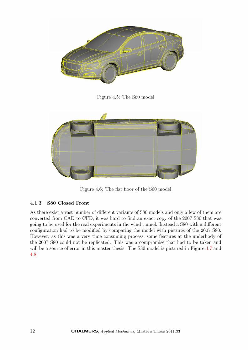
Figure 4.5: The S60 model

Figure 4.6: The flat floor of the S60 model

4.1.3 S80 Closed Front

As there exist a vast number of different variants of S80 models and only a few of them areconverted from CAD to CFD, it was hard to find an exact copy of the 2007 S80 that wasgoing to be used for the real experiments in the wind tunnel. Instead a S80 with a differentconfiguration had to be modified by comparing the model with pictures of the 2007 S80.However, as this was a very time consuming process, some features at the underbody ofthe 2007 S80 could not be replicated. This was a compromise that had to be taken andwill be a source of error in this master thesis. The S80 model is pictured in Figure 4.7 and4.8.


Figure 4.7: The S80 closed front model

Figure 4.8: The floor of the S80 closed front model

To do a closed front simulation, the upper and lower grill was closed of by a flat surfacein order to stop air from entering the engine bay. The engine bay was also sealed at thebottom by flat surfaces which effectively meant that no part of the engine bay would beused for the closed front simulation, all according to computational procedure AEDCAE01[5].

4.1.4 S80 Open Cooling

In the Open Cooling case the grills were left open and the air was let through the coolingpack and engine bay area. The cooling pack consisted of the main fans and radiators inthe same detail as standard open cooling simulations performed at Volvo Cars [6]. This ishowever more simple than a real production car which have even more objects and partsin the engine bay and cooling pack area. The geometry of the grill and part of the enginebay can be seen in Figure 4.9, where the left side of the exterior has been removed.


Figure 4.9: Front view of the S80 open cooling model

4.2 Mesh

4.2.1 PVT Tunnel

The volume mesh was created with Harpoon, with the maximum cell size set to 160 mm.To resolve the geometry as good as possible the smallest cell used was 5 mm. The meshdistribution of the symmetry plane can be seen in Figure 4.10.

Figure 4.10: Mesh distribution of the symmetry plane

In order to keep y+ between 30 and 500, three prism layers with a first layer height of2 mm were added to the volume mesh. Since prism layers is hard to produce in Harpoonwith good quality even for simple geometries, they were restricted to the area around thetest section, hence to the slotted walls, diffuser, floor and part of the nozzle closest to thetest section. In a optimal case, the prism layer height would have been varied dependingof the velocity at the walls in order to always keep y+ close to 30. However, this was notpossible to do in Harpoon in a simple way and instead an approximated height of 2 mmwas chosen. A height of 1 mm had been tested but produced y+ values well below 30 in


some areas, which was not adequate. The resulting y-plus of the walls is presented byFigure 4.11. Where there are prism layers y+ is approximately between 30 and 150.

Figure 4.11: y+ on the walls of the tunnel

When creating the prism layers, care had to be taken to the area around the nozzle,due to the accelerating flow and thus increasing friction velocity. When looking at someearly simulation results there were no distinctive line where the prism layers were needed,therefore the prism layers creation was started at an approximated position at the centerof the nozzle. This was a compromise but the easiest and quickest way of producing fairlyaccurate results.

In the beginning the surface cell sizes were only small enough to resolve the geometrybut convergence problems which was believed to be mesh related forced the surface cell sizesto be decreased and refinement zones to be added. A large refinement box where addedwhich enclosed the whole test section within the slotted walls and small boxes where addedat the rear of the slotted walls, in between the slots. The resulting number of cells for theempty tunnel ended at 78 million. In the end the convergence problems showed not to bedue to a too coarse mesh but because of wrongly defined boundary conditions. The fineresolution was kept anyway as the number of cells was still below a plausible level.

4.2.2 S60

When setting up the meshing settings for the S60 , the normal procedure at Volvo Carsfor an aerodynamic simulation was followed [5]. It was important that the cell sizes of thecar surfaces and the density boxes around the car was essential the same as the normalcase performed at Volvo Cars. The resulting surface cell sizes of the car ranged from 5 mmdown to 1.25 mm. The mesh quality and the surrounding refinement boxes is displayed inFigure 4.12.


Figure 4.12: Mesh distribution across the symmetry plane of the S60

As no prism layers is used, y+ becomes sensitive to the level of refinement needed toresolve the car geometry. This can be seen in Figure 4.13 where the lowest values y+ isfound at refined areas such as the rear of the car and the a-posts. Mostly, y+ is around250 and never goes lower than the laminar limit which correspond to a y∗ value of 11.225.Figure 4.13 also shows another consequence of having no prism layers as the mesh methodapplied by Harpoon creates fictitious oval patterns across the surface of the car.

Figure 4.13: y+ on the S60

In order to keep the amount of cells down to a acceptable level, the surface cell sizes ofthe PVT tunnel was decreased without compromising the resolution of the geometry. Thismeant that the number of cells for the tunnel with the S60 was kept at 65 million insteadof being well above 100 million.

4.2.3 S80 Closed Front

The volume mesh for the S80 was created with the same PID distribution, surface cell sizesand refinement boxes which had been used in previous simulations of the S80, the sameapproach as for the S60 [5]. This meant that four refinement boxes was added, where one


large refinement box covered the whole car, one enclosed the area under the car and thetwo other was placed at the rear and the wake of the car. The cell distribution around thecar and across the symmetry plane is showed in Figure 4.14. The detailed floor increasedthe cell count heavily resulting in a volume mesh of 76 million cells.

Figure 4.14: Mesh distribution across the symmetry plane of the S80 closed front

The surface cell sizes ranged from 5 mm to 1.25 mm, a resolution which resulted in they+ distribution showed in Figure 4.15. Just as for the S60, y+ is sensitive to the degree ofrefinement and the same fictitious oval patterns are created on the surface of the S80.

Figure 4.15: y+ on the S80

4.2.4 S80 Open Cooling

Since also the fully detailed grill, spoiler opening and engine bay area were included in theS80 open cooling model, the cell count inevitably became a lot higher compared to theclosed front model due to the small cell size needed to resolve the complicated geometryand the total cell count ended at 114 million cells. The symmetry plane of the engine bayarea of the S80 is shown in Figure 4.16 and a refinement box around the cooling package


is visible as the more black and dense area. However, this refinement box was omitted bymistake in the PVT simulation and was only included in the simulation of the CFD tunnel.

Figure 4.16: Mesh distribution across the symmetry plane of the S80 engine bay

As the S80 open cooling had the same level of refinement of the exterior as the closedfront version, it had also the same y+ distribution across the surface, thus no new figure isneeded here, instead see Figure 4.15.

4.3 Calculation Settings

In the PVT tunnel the velocity is calculated from the pressure difference(dp) in the nozzle,measured by the two pressure taps PC1 and PC2. PC1 is located just before the contractionof the nozzle and PC2 is located after the contraction, before the test section, as shown byFigure 4.17.

Figure 4.17: Locations of PC1 and PC2 on the nozzle roof

In the figure, the pressure taps are located at the centre line of the nozzle but in realitythere are two pressure taps on each side of the centre line and the pressure is taken as theaverage between these two positions. However, results showed that the pressure did not


vary in any significant magnitude in the y direction and only one position at the centre linewas used for most of the simulations. From dp, PC1 and PC2 the calibration coefficientskp and kq are calculated through equations 4.1 and 4.2, where Ps and Pt is the static andtotal pressure at the position where the desired velocity is calibrated.

kp =Ps − PC2

PC1 − PC2

(4.1)

kq =Pt − Ps

PC1 − PC2

(4.2)

When the tunnel was calibrated by Aiolos [7], a pitot tube was placed in center of theturntable measuring the static and dynamic pressure, 1.2 meters above the floor, makingit possible to calculate the calibration coefficients for different velocities. This gave acorrelation between dp in the nozzle and the velocity in the test section for each differentconfiguration of the tunnel. The resulting polynomial coefficients for the equation b*dp+awhich is used to calculate the calibration coefficients for each configuration is shown in thetables below.

Table 4.1: The calibration coefficients for Scoop only modeCoefficient a b

kp 0.047052534 -0.000002348kq 0.971833432 0.000003161

Table 4.2: The calibration coefficients for GESS off modeCoefficient a b

kp 0.060246216 -0.000002456kq 0.958619998 0.000003841

Table 4.3: The calibration coefficients for Aerodynamic modeCoefficient a b

kp 0.063270435 -0.000004086kq 0.958670736 0.000003667

When a car is inside the tunnel it is impossible to measure the velocity at the center ofthe turn table as that is where the car is positioned. Instead the velocity is calculated byusing the calibration coefficients and the pressures measured at the contraction taps, PC1

and PC2. In order to achieve a certain velocity in the test section with a car inside, dp isset to the same dp which produced the sought velocity in an empty tunnel.

However, since the CFD-simulation produced different dp than the real PVT, the realcalibration coefficients could not be used in the CFD as they gave an incorrect velocityin the test section. Also, when performing half tunnel calculations for different velocities,the real calibration coefficient was found to produce incorrect Cp plots. In Figure 4.18, Cp,calculated with Aiolos calibration coefficients, is plotted for four different velocities alongthe center line of the test section at a height of 600 mm. The calibration coefficients merelytranslates the Cp upwards for decreasing velocity and does not counteract the decrease in


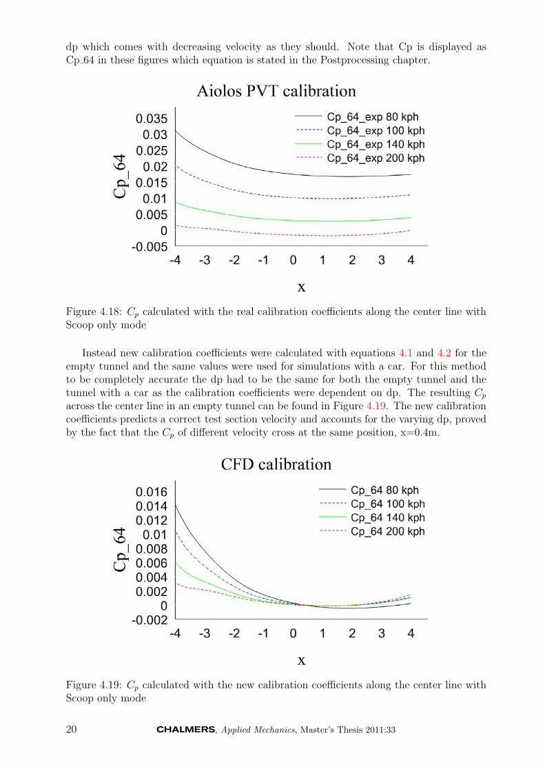
dp which comes with decreasing velocity as they should. Note that Cp is displayed asCp 64 in these figures which equation is stated in the Postprocessing chapter.

Figure 4.18: Cp calculated with the real calibration coefficients along the center line withScoop only mode

Instead new calibration coefficients were calculated with equations 4.1 and 4.2 for theempty tunnel and the same values were used for simulations with a car. For this methodto be completely accurate the dp had to be the same for both the empty tunnel and thetunnel with a car as the calibration coefficients were dependent on dp. The resulting Cp

across the center line in an empty tunnel can be found in Figure 4.19. The new calibrationcoefficients predicts a correct test section velocity and accounts for the varying dp, provedby the fact that the Cp of different velocity cross at the same position, x=0.4m.

Figure 4.19: Cp calculated with the new calibration coefficients along the center line withScoop only mode


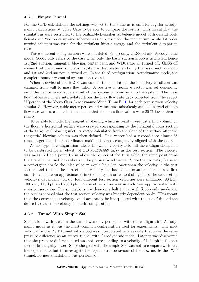
4.3.1 Empty Tunnel

For the CFD calculations the settings was set to the same as is used for regular aerody-namic calculations at Volvo Cars to be able to compare the results. This meant that thesimulations were restricted to the realizable k-epsilon turbulence model with default coef-ficients and 2nd order upwind schemes was only used for the momentum, while 1st orderupwind schemes was used for the turbulent kinetic energy and the turbulent dissipationrate.

Three different configurations were simulated, Scoop only, GESS off and Aerodynamicmode. Scoop only refers to the case when only the basic suction scoop is activated, hence1st/2nd suction, tangential blowing, center band and WDUs are all turned off. GESS offmeans that the ground simulation system is deactivated and only the basic suction scoopand 1st and 2nd suction is turned on. In the third configuration, Aerodynamic mode, thecomplete boundary control system is activated.

When a device of the BLCS was used in the simulation, the boundary condition waschanged from wall to mass flow inlet. A positive or negative vector was set dependingon if the device would suck air out of the system or blow air into the system. The massflow values set where interpolated from the max flow rate data collected from the report”Upgrade of the Volvo Cars Aerodynamic Wind Tunnel” [1] for each test section velocitysimulated. However, cubic meter per second values was mistakenly applied instead of massflow rate values, a mistake that meant that the mass flow values were 20 % lower than inreality.

To be able to model the tangential blowing, which in reality were just a thin column onthe floor, a horizontal surface were created corresponding to the horizontal cross sectionof the tangential blowing inlet. A vector calculated from the slope of the surface after thetangential blowing column was then defined. This vector had a x-coordinate almost 68times larger than the z-coordinate, making it almost completely aligned with the floor.

As the type of configuration affects the whole velocity field, all the configurations hadto be calibrated for a velocity of 140 kph(38.889 m/s) in the test section. The velocitywas measured at a point 1.2 m above the center of the turn table, the same position asthe Prantl tube used for calibrating the physical wind tunnel. Since the geometry featureda convergent nozzle the inlet velocity would be a lot lower than the velocity in the testsection and to find the correct inlet velocity the law of conservation of mass was firstused to calculate an approximated inlet velocity. In order to distinguished the test sectionvelocity’s dependency on dp, four different test section velocities were simulated; 80 kph,100 kph, 140 kph and 200 kph. The inlet velocities was in each case approximated withmass conservation. The simulations was done on a half tunnel with Scoop only mode andthe results showed that the test section velocity was linearly dependent on dp. This meantthat the correct inlet velocity could accurately be interpolated with the use of dp and thedesired test section velocity for each configuration.

4.3.2 Tunnel With Simple S60

Simulations with a car in the tunnel was only performed with the configuration Aerody-namic mode as it was the most common configuration used for experiments. The inletvelocity for the PVT tunnel with a S60 was interpolated to a velocity that gave the samepressure difference as an empty tunnel with Aerodynamic mode. Later it was discoveredthat the pressure difference used was not corresponding to a velocity of 140 kph in the testsection but slightly lower. Since the goal with the simple S60 was not to compare with reallife experiments but to investigate the asymmetric behaviour of the flow inside the PVTtunnel, no new simulations was performed.


4.3.3 Tunnel With S80 Closed Front

The S80 was at first only simulated with Aerodynamic mode, but a simulation with thetangential blowing turned off was later also performed. This was done by simply changingthe boundary condition of the tangential blowing from inlet mass flow to wall. The velocityat the inlet was interpolated in the same way as for the S60 to give the same pressuredifference across the nozzle as the empty tunnel.

To accurately simulate the rotation of the real rims which the S80 model incorporated,MRF zones was used, which meant that the fluid in between the spokes was rotated alongwith the surfaces of the rim which were tangential to the flow direction, according tocomputational procedure AEDCAE01 [5].

4.3.4 Tunnel With S80 Open Cooling

The inclusion of the cooling package in the S80 open cooling modelled meant that thepressure drop and the rotating fans had to be accounted for. The pressure drop was takenfrom measurements and simple specified in Fluent by the radiator boundary condition. Themovement of the two fans was modelled in almost the same way as the rotating wheels, thuswith MRF zones, difference being that the complete zone enclosing the fan was rotatedand not just only the fluid in between the fan blades.

4.4 Postprocessing

When comparing CFD results with experimental results it is very important that thevariables are normalized in the same way in both CFD and the experiments. NormallyCp is calculated using a free stream static pressure and the free stream dynamic pressureaccording to equation 4.3.

Cp =P − Ps,ref

qref(4.3)

But since the reference pressures is hard to define in the PVT tunnel Cp have to becalculated in a different way. Instead of the standard definition, Cp was calculated withthe use of the calibration coefficients together with dp and PC2. The PVT Cp equation isdisplayed in equation 4.4 and this Cp equation is referred to Cp 64 in figures and graphsthroughout this report.

Cp =P − PC2

(PC1 − PC2) ∗ kq −kpkq

(4.4)

To be able to compare the dynamic pressure uniformity in an empty tunnel with ex-periments performed by Aiolos, the dynamic pressure was calculated in the same way asin the experiments. The equation used by Aiolos is shown by equation 4.5, where k=1.4.As the pressures needed to be in absolute values, the reference pressure of 101325 Pa usedin the CFD was added to the static values. The dynamic pressure was then normalizedin the CFD by the free stream dynamic pressure taken at the center of the turn table atz=1.2m. This was somewhat different than in the experiments where the facility evaluatedtest section dynamic pressure was used.

q =k

k − 1∗ Ps ∗ (Pt − Ps

Ps

k−1/k− 1) (4.5)


During James C. Lyon’s master thesis [8], where wind tunnel experiments were com-pared with coast down tests on the open road through pressure taps on the center line ofthe car, a different way of calculating Cp was used where the reference pressures were takenat the hood of the car, close to the windscreen, and in front of the car. The same definitionof Cp was therefore applied on the CFD results in order to be able to compare them withthe results from James C. Lyon’s experiments. Despite using the same stated positionsfor the reference pressures as described, the result showed to be very different and notcompletely believable so instead the PVT definition, equation 4.4 was used for the CFDresults. Also, the exact positions of the pressure taps used during the experiments was notknown and instead they were arbitrary placed by looking at the center line pressure plotsof the experiments. Due to large gradients in certain areas of the car, a slight change inthe position of a pressure point could change Cp considerably. This will have to be kept inmind when analyzing this comparison in the result section.


5 Results and Discussion

The results in this chapter are presented in the same order as in chapter 4, Method; firstempty tunnel, then tunnel with S60 and last tunnel with S80.

5.1 Empty Tunnel

5.1.1 Asymmetrical Behaviour

In the beginning of this master thesis it was important to control if it was possible to onlydo calculations on one half of the tunnel, thus saving simulation time. However, it wasquickly understood that the geometry of the PVT tunnel was far too asymmetrical andonly simulating one half would not be sufficient due to the loss of information.

A good way to show that the asymmetrical slotted walls support have a big effect onthe flow field is by plotting the pressure on the slotted walls. In Figure 5.1 the contour ofthe pressure is plotted on the right side of the slotted walls for Aerodynamic mode. Noticethat the pressure drops at the smaller support beams and at the middle large beam. Thescale is however very small, only a few pascals. The left side is shown in Figure 5.2 andthe difference is quite significant. Here there are no small pressure drops as the smallersupport beams are absent.

Figure 5.1: Pressure at the right wall in an empty tunnel with Aerodynamic mode


Figure 5.2: Pressure at the left wall in an empty tunnel with Aerodynamic mode

The asymmetry is even more evident when plotting Cp across one of the horizontalbeams as shown in Figure 5.3. Usually when experiments is made and the aim is toexamine the pressure on the slotted walls, pressure taps is placed on the 2nd horizontalbeam element from the floor. To be able to compare the CFD with the experiments thesame beam element was used. The black line in Figure 5.1 and 5.2 represents the linewhich Cp is plotted along in the following figures.

As can be seen by Figure 5.3, the difference between the right wall and left wall ispretty obvious. The four additional vertical support beams on the right side have a largeimpact on the flow inside the slotted wall. Instead of being smooth as on the left side, thecurve is disturbed by the support beams and the pressure drops at each beam.

Figure 5.3: Cp at the wall in an empty tunnel with Aerodynamic mode

The four additional support beams is however not the only difference between the rightand left side. As can be noticed in Figure 5.3 there is also a pressure drop between thepair of support beams where the drop is bigger on the right wall compare to the left wall.This is because the main vertical support beam which is found on both sides is different


on the right side. On the right side it has the same triangulated elements connecting itto the slotted walls as the additional support beams have which are different from thesolid squared ones on the left side. The asymmetrical behaviour in the wind tunnel will befurther investigated with a car inside the tunnel later in this report.

5.1.2 Axial pressure gradient

It is a known fact that when the PVT tunnel is empty, it has a positive axial pressuregradient across the test section. A positive axial pressure gradient means that the pressureis higher at the area where a car’s front normally is situated compared to the area wherea car’s rear and wake is placed. This will affect the pressure distribution on a car in thetunnel in a way which increases the measured drag. Figure 5.4 shows Cp along the centerline for four different heights and for Aerodynamic mode. It is clear from the figure thatthe PVT tunnel has positive axial pressure gradient.

Figure 5.4: The axial pressure gradient across the center line for Aerodynamic mode

5.1.3 Nozzle Contraction

As PC1 and PC2 have a large impact on the way Cp is calculated, the pressure drop of thenozzle was examined. In Figure 5.5 the static pressure along the centerline of the roof of thenozzle for Scoop only mode is plotted. One would expect the pressure to drop consistentlyas the nozzle contracts and then at the end smoothly even out to a constant motion, butthis is obviously not the case here. Instead the pressure curve reach its minimum at x=-7.8m and then start to rise again before it rather chaotic assumes a constant behaviour.Evidently the flow separates here and the velocity decreases after the pressure minimuminstead of continue to increase or become constant. The geometry of the nozzle does notseem to be as good as required to keep a good flow through the nozzle.


Figure 5.5: Pressure at nozzle roof with Scoop only mode

Since PC2 is positioned at x=-7.25, which is not where the pressure reaches its mini-mum, the pressure difference between PC1 and PC2 will not be equal to the true pressuredifference over the nozzle. Also, if a steady simulation produces a curve like this, then it ispossible that the pressure at PC2 in the real tunnel can have a non desired time dependentfluctuating behaviour.

To show that this results was due a non optimal geometry and not because of anyCFD related error, for example a bad mesh, a new nozzle was designed which had a longercontraction than the original. To simplify the simulation and remove any impact of otherobjects in the tunnel like the suction scoop, the tunnel was turned into a solid walls tunnel.The difference between the original nozzle and the new nozzle can be seen in Figure 5.6where the static pressure along the roof is plotted.

Figure 5.6: Pressure at nozzle roof

The new nozzle have a much smoother pressure curve because of the more forgivingcontraction. The small bump experienced by both nozzles is situated where the surface


becomes horizontal. Refinements of the mesh at this area did not smoothen out the bumpand therefore it can be concluded that it is not mesh related. Regardless, there is no doubtthat the new nozzle would be a better solution than the original as the pressure drop ismore consistent.

5.1.4 Comparison With Experiments

When comparing the CFD results with real experiments in the tunnel a big difference canbe noticed, namely the magnitude of the pressure differences in the domain. In the CFDthe pressure differences is a lot smaller than in the experiment. For example, Cp along the2nd beam element fluctuates at the support beams with a magnitude of 0.002 in the CFD.In the experiments the magnitude of the fluctuations is a lot higher, more than 0.05. Thebig difference can be seen in Figure 5.7 and in comparison the CFD curve becomes almostlike a straight line.

Figure 5.7: Cp at wall in an empty tunnel

Such a large difference was not expected and the reason behind it is not so easily ex-plained. The flow in the PVT tunnel is natural unsteady and enforcing a natural unsteadyflow field to give a steady solution as in the CFD simulation means that information is lostmainly due to time-averaging, but also because of the solver’s habit of suppressing unsteadybehaviour in order to produce better convergence. But the experiments is time-averagedas well which means that other factors must be behind the difference.

Another factor which effects the results is the uniformity of the flow. Figure 5.8 and5.9 compares the normalized dynamic pressure from the CFD simulation with the mea-surements made by Aiolos [7], both with Aerodynamic mode, in two planes at x-position-2500mm and x-position 2500mm. The flow in the CFD simulation is a lot more uniformthan in the experiment which could be the reason why the pressure felt by the slotted wallsis of less varying degree.


Figure 5.8: Dynamic pressure uniformity at x=-2500 mm

Figure 5.9: Dynamic pressure uniformity at x=2500 mm

But then the question arise why the CFD simulation predicts a more uniform flow thanwhat is measured in the experiments? An important reason that cannot be underestimatedis the absence of the PVT tunnel’s closed air path which have been left out as the simulatedgeometry has been restricted to the nozzle, test section and diffuser. Even tough turningvanes and turbulence nets are used in the PVT tunnel to make the flow as uniform aspossible the flow will inevitable inhabit some non-uniformity when it reaches the nozzle.This non-uniformity is not accounted for in the CFD simulation due to the geometryrestrictions and instead a uniform velocity field is enforced at the nozzle inlet, whichobviously in not a completely accurate imitation of the true flow conditions.

To find other reason behind the uniformity difference it is interesting to examine howwell the CFD modeling of the near wall flow compare to the near wall flow in the experi-ments. When PVT was calibrated, Aiolos measured the boundary layer at several locationson the floor across the turn table. Four of the locations is illustrated in Figure 5.10 on atop view sketch of the turn table with the center belt, WDUs and 2nd suction zone marked.Note that area around position x=-2710 mm, which represent stationary floor, is larger onthe sketch than in reality. Also, in reality there is a small gap between the static floor andthe leading edge of the center belt. In the CFD the static floor and the gap does not existand the 2nd suction zone directly transcends to the center belt.


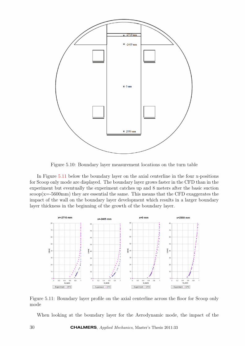
Figure 5.10: Boundary layer measurement locations on the turn table

In Figure 5.11 below the boundary layer on the axial centerline in the four x-positionsfor Scoop only mode are displayed. The boundary layer grows faster in the CFD than in theexperiment but eventually the experiment catches up and 8 meters after the basic suctionscoop(x=-5600mm) they are essential the same. This means that the CFD exaggerates theimpact of the wall on the boundary layer development which results in a larger boundarylayer thickness in the beginning of the growth of the boundary layer.

Figure 5.11: Boundary layer profile on the axial centerline across the floor for Scoop onlymode

When looking at the boundary layer for the Aerodynamic mode, the impact of the


static floor and the gap between the 2nd suction zone and the center belt is obvious. Inthe experiment the leading edge of the center belt creates a momentum deficit with a largevelocity magnitude across a small height. When it propagates down the center belt themagnitude gets smaller with an increasing height as the flow catches up. As the PVT modelin the CFD is simplified with a completely flat floor, this velocity deficit is non-existentdue to the absence of any geometry triggering it and the boundary layer never developsalong center belt.

Figure 5.12: Boundary layer profile on the axial centerline across the floor for Aerodynamicmode

The simplification of the floor and the resulting absence of a boundary layer alongthe center belt is a factor that will help keep the flow uniform. As the simplification ofthe geometry in the CFD simulation is not restricted to only the floor, but is performedthroughout the whole domain, there is a chance that important geometries have been leftout which would have had a big influence on the uniformity of the flow and consequentlythe pressure on the slotted walls.

The discovery of the somewhat irregular pressure drop along the roof center line of thenozzle prompted a brief examination to be made during the experiments performed by ErikLindmark [9]. Four pressure taps was placed 500 mm to the left of the center line, withthe first tap placed 50 mm before PC2, the second tap at the same x-position as PC2 andthe last two after PC2. The position of the pressure taps can be seen in Figure 5.13. Theallocation of the pressure tap before PC2 was limited by how far it was possible to reachwith the help of the available ladder.


Figure 5.13: Pressure taps on the nozzle roof

The resulting graph of Cp along the pressure tap for an empty tunnel is displayed inFigure 5.14. The graph shows that the pressure reaches its minimum at the pressure tapplaced close to Cp, different from the CFD results where the minimum was found 550 mmbefore PC2. However, in the CFD results the pressure along the whole length of the nozzleroof was plotted and in the experiment only one pressure tap was positioned before PC2,which is not enough to give a true picture of the change in pressure across Cp. The valuesof Cp is also worryingly high, far from zero when they should be close to zero, especially thesecond pressure tap, so it is recommended to perform further measurement of the nozzlepressure.

Figure 5.14: Cp on the nozzle roof from experiments

Up till now, only the weaknesses of the CFD simulation have been discussed as reasonsbehind the difference compared to the experiments and no thought have been put on theerrors that comes with the measuring technique during the experiments. These are however


many and sometimes severe but going through them here would demand too much time andspace. For sources of error in the experiments performed by Aiolos see the Commissioningreport [7].

5.2 Tunnel With Simplified S60


The asymmetrical geometry’s impact on the flow field is more clear when a car is inside thetunnel. Figure 5.15, where Cp is plotted across the 2nd beam element of the slotted walls,shows that the difference between the right and left side is more significant than withouta car in the tunnel.

Figure 5.15: Cp at slotted walls with a S60

By looking at the wake of the car the impact of the asymmetry on the flow aroundthe car can be distinguished. In Figure 5.16 the wake 100 mm meters behind the rear ofthe car is plotted. The wake shows that there is a larger inflow from the left side of thetunnel. Since the flow tends to always move to the area of lowest pressure, more mass flowflows through the slotted walls on the left side of the car where there is less blockage thanon the right side. This leads to that more air can flow in behind the car on the left sidethan on the right side, thus resulting in a asymmetric wake. This is further emphasizedby Figure 5.17 which is the wake 1000 mm behind the rear of the car. The wake is evenmore asymmetric here.


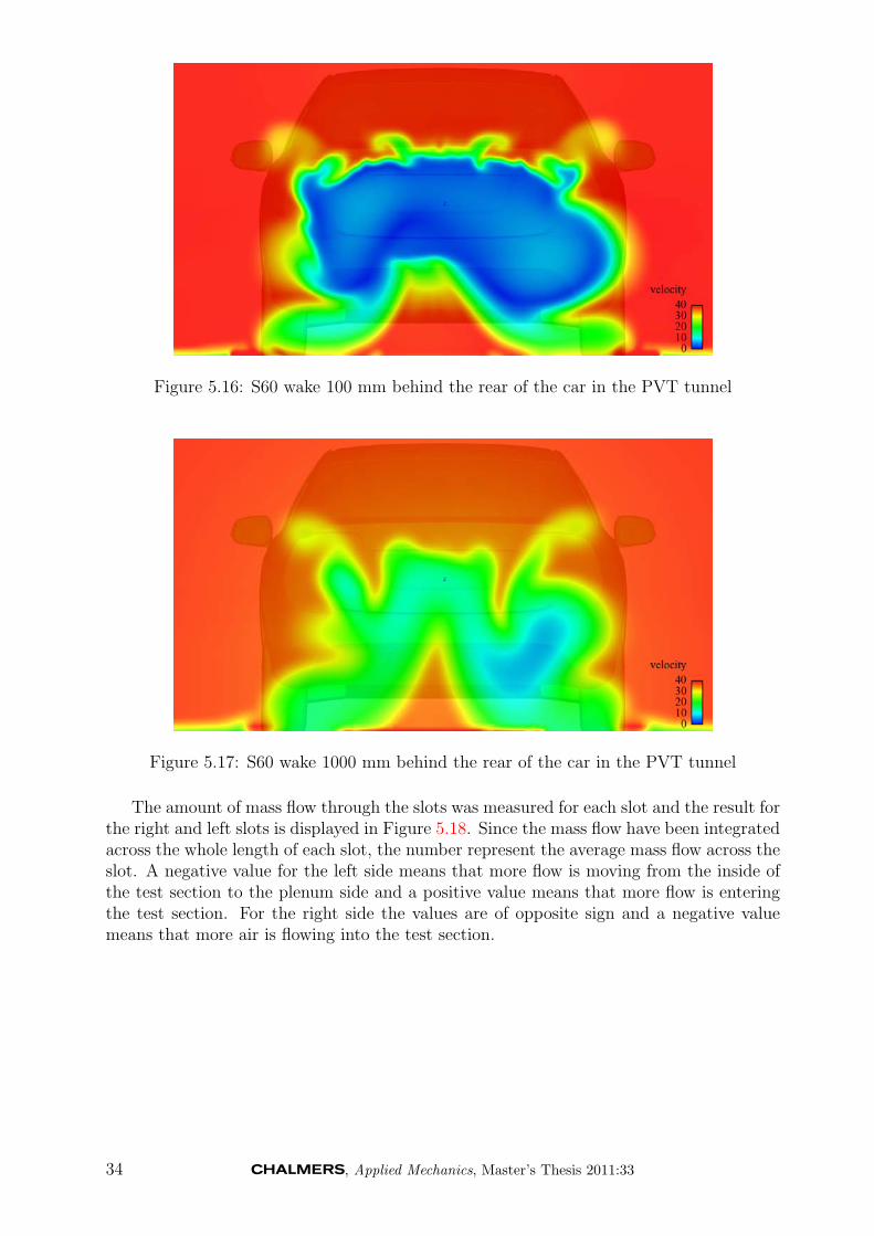
Figure 5.16: S60 wake 100 mm behind the rear of the car in the PVT tunnel

Figure 5.17: S60 wake 1000 mm behind the rear of the car in the PVT tunnel

The amount of mass flow through the slots was measured for each slot and the result forthe right and left slots is displayed in Figure 5.18. Since the mass flow have been integratedacross the whole length of each slot, the number represent the average mass flow across theslot. A negative value for the left side means that more flow is moving from the inside ofthe test section to the plenum side and a positive value means that more flow is enteringthe test section. For the right side the values are of opposite sign and a negative valuemeans that more air is flowing into the test section.


Figure 5.18: Mass flow through the slots on the right and left side

The figure shows that the more flow is leaving the test section than entering it on theright side for all slots. For the left side the opposite occur for slot number 2 to 4 countedfrom the ground, where number 2 is roughly situated at the waist line of the car and theother two above. This indicates the reason behind the large inflow on the left side, butto get the whole picture it is convenient to look at the elevated surfaces of the mass flowthrough the slots which is showed by Figure 5.19. The flow is coming back behind the carin a larger scale on the left side compare to the right side which have resulted in the veryasymmetric wake.

Figure 5.19: Mass flow through the slots represented by elevated surfaces

Shown below in Figure 5.20 and 5.21 is the wake of the car in an ordinary CFD tunnel,which is a large rectangular box with symmetry boundary conditions. The ordinary CFDsimulation have also a complete moving ground system instead of a 5-belt system. Thewake is here very symmetric which is expected as the car itself is symmetric. The differencebetween the CFD tunnel and PVT tunnel is quite large, a difference which is not desirable.


Figure 5.20: S60 wake 100 mm behind the rear of the car in the CFD tunnel

Figure 5.21: S60 wake 1000 mm behind the rear of the car in the CFD tunnel

During experiments in the PVT tunnel there have always been a difference in yawingthe car to the left compared to yawing it to the right. With cars with asymmetric floor thiscould be expected but the difference have been large and the asymmetric floor cannot bethe sole reason. Since the CFD simulations have shown that the asymmetric slotted wallsin the PVT tunnel have a large impact on the flow, there is good reason to believe thatthe resulting asymmetry in the flow could be a contributing factor. Therefore simulationswas performed with the S60 yawed 20◦ to the right and yawed 20◦ to left. Despite the carbeing symmetric, Figure 5.22 shows a clear difference between the direction of yawing.


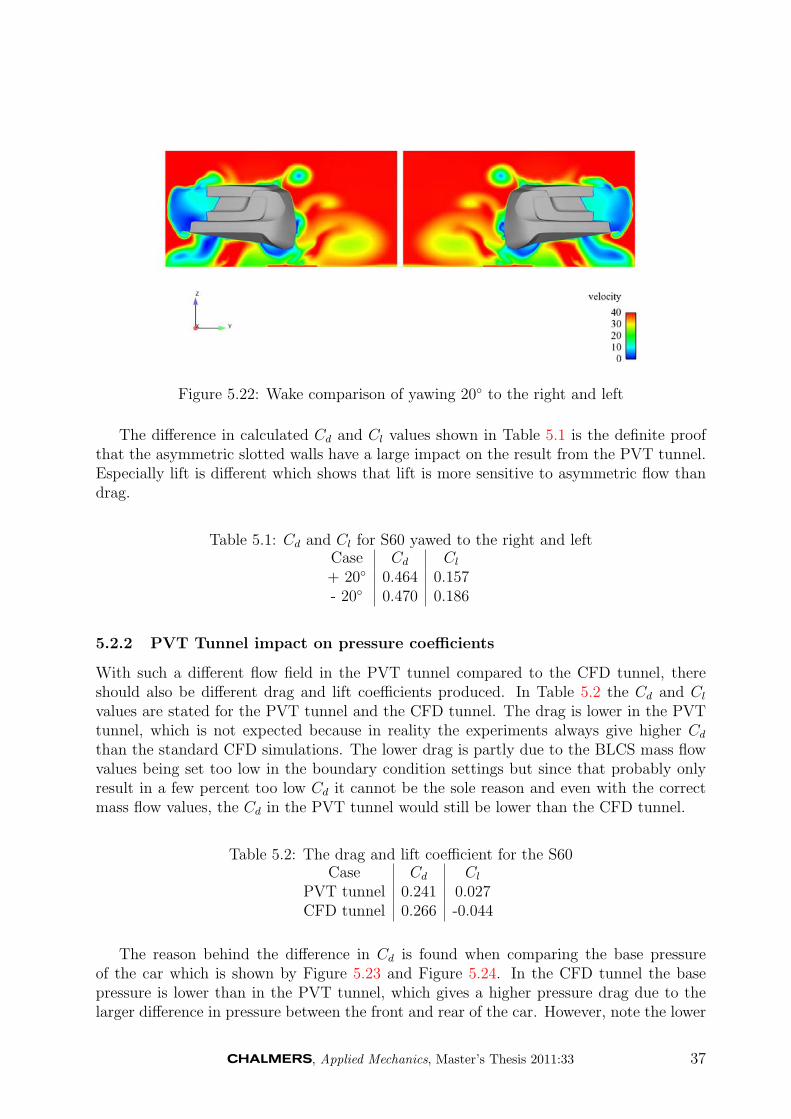
Figure 5.22: Wake comparison of yawing 20◦ to the right and left

The difference in calculated Cd and Cl values shown in Table 5.1 is the definite proofthat the asymmetric slotted walls have a large impact on the result from the PVT tunnel.Especially lift is different which shows that lift is more sensitive to asymmetric flow thandrag.

Table 5.1: Cd and Cl for S60 yawed to the right and leftCase Cd Cl

+ 20◦ 0.464 0.157- 20◦ 0.470 0.186

5.2.2 PVT Tunnel impact on pressure coefficients

With such a different flow field in the PVT tunnel compared to the CFD tunnel, thereshould also be different drag and lift coefficients produced. In Table 5.2 the Cd and Cl

values are stated for the PVT tunnel and the CFD tunnel. The drag is lower in the PVTtunnel, which is not expected because in reality the experiments always give higher Cd

than the standard CFD simulations. The lower drag is partly due to the BLCS mass flowvalues being set too low in the boundary condition settings but since that probably onlyresult in a few percent too low Cd it cannot be the sole reason and even with the correctmass flow values, the Cd in the PVT tunnel would still be lower than the CFD tunnel.

Table 5.2: The drag and lift coefficient for the S60Case Cd Cl

PVT tunnel 0.241 0.027CFD tunnel 0.266 -0.044

The reason behind the difference in Cd is found when comparing the base pressureof the car which is shown by Figure 5.23 and Figure 5.24. In the CFD tunnel the basepressure is lower than in the PVT tunnel, which gives a higher pressure drag due to thelarger difference in pressure between the front and rear of the car. However, note the lower


pressure on the back of the rear wheels when the car is in the PVT tunnel. The causebehind this will be investigated with the S80 in the tunnel.

Figure 5.23: Cp at rear of the S60 in the PVT tunnel

Figure 5.24: Cp at rear of the S60 in the CFD tunnel

The difference in lift is more expected as the simulation of the moving ground is differentin the two cases. In the PVT tunnel the open road conditions is simulated by a 5-beltmoving ground system and a boundary control system, with different suction zones andtangential blowing. This is very different from the CFD tunnel where the complete groundis set as moving. In order to investigate the impact of the floor in the PVT tunnel anew simulation was performed with the whole floor inside the slotted walls set as movingground, the same floor boundary condition as in the CFD tunnel. The basic scoop waskept because turning it off would have given strange results due to the large stagnationarea created. However, this was only done early in the project with a coarse mesh withoutany refinement boxes around the S60, which means that the accuracy of the simulations islower. Table 5.3 shows the drag and lift coefficients for the simulation with Aerodynamicmode and the simulation with complete moving ground.


Table 5.3: Cd and Cl for Aerodynamic mode compared with complete moving groundCase Cd Cl

PVT Aerodynamic mode 0.248 0.030PVT Complete moving ground 0.257 0.016

The table confirms that the lift coefficient depends largely on the type of moving groundsimulation system used. The 5-belt system does not fully simulate moving road conditionsand despite using tangential blowing to ”fill in” the boundary layer between the wheels, ahigher Cl is obtained. That the opposite happen for the drag coefficient is not as easy toexplain because a larger area of moving ground should decrease Cd. However, the changefrom Aerodynamic mode to complete moving ground means also that it is less suctioninside the domain and that influences the flow field. The reason behind the lower Cd withAerodynamic mode will be further investigate with the S80 in the tunnel.

5.3 Tunnel With S80 Closed Front


Figure 5.25 shows that just as the simple S60, the S80 increases the difference of Cp onthe right side compared to the left side of the slotted walls. Compared to the S60 thelargest difference is found at the end of the walls, which implies that the wake structureis different. That is something which is expected as the S80 has a different body and adetailed, unsymmetrical floor.

Figure 5.25: Cp at slotted walls with a S80

What was not expected tough, was that the wake of the S80 would be more symmetricin the PVT tunnel compared to the CFD tunnel. The results from the PVT tunnel isshown by Figure 5.26 and Figure 5.27 and the results from the CFD tunnel is shown inFigure 5.28 and Figure 5.29. The difference is most notable at the top and bottom of thewake, which represents the flow coming from over and under the car. It seems like theasymmetry of the slotted walls even out the effect of the asymmetric floor and vice versa.There is no large inflow from the left side like in the case with the S60. Apparently someof the information regarding the asymmetry of the flow around a car is lost in the PVTtunnel.


Figure 5.26: S80 wake 100 mm behind the rear in the PVT tunnel

Figure 5.27: S80 wake 1000 mm behind the rear in the PVT tunnel

Figure 5.28: S80 wake 100 mm behind the rear in the CFD tunnel


Figure 5.29: S80 wake 1000 mm behind the rear in the CFD tunnel

This is further emphasized by Figures 5.30 and 5.31 where Cp on the top of the car isplotted. At the windscreen junction the pressure on the car is very symmetric when thecar is in the PVT tunnel, but less so in the CFD tunnel. The impact of the tunnel wallsis in this case counter productive and the results from the PVT tunnel does not give acompletely true picture of the flow around the car.

Figure 5.30: Cp on the top of the S80 in the PVT tunnel


Figure 5.31: Cp on the top of the S80 in the CFD tunnel

In order to investigate the tangential blowing’s effect on the drag, covered in the nextchapter, a new simulation was performed with the tangential blowing turned of. As sup-ported by Figure 5.32, where the wake 100 mm behind the rear of the car is shown, withoutthe tangential blowing the flow coming from the top of the car is a lot more asymmetric.The vortexes which is created by the radio antenna on the roof is different on the left sidecompared to the right.

Figure 5.32: S80 wake 100 mm behind the rear in the PVT tunnel with the tangentialblowing deactivated


From earlier experience at Volvo Cars the CFD calculations always produced lower Cd

values than the experiments in the PVT tunnel. It should therefore be expected that thesimulation of the PVT tunnel would give a higher Cd than the simulation of a CFD tunnel.However, the result follow the same pattern as the S60 and the S80 in the PVT simulationhave a lower Cd than in the CFD simulation. The Cd and Cl values are shown in Table5.4.


Table 5.4: The drag and lift coefficient for the S80, PVT tunnel versus CFD tunnelCase Cd Cl

PVT tunnel 0.279 0.135CFD tunnel 0.284 0.127

One of the reason behind the higher Cd in the CFD tunnel is because of the lower basepressure on the car. The base pressure of the PVT tunnel and the CFD tunnel is shown inFigure 5.33 and Figure 5.34 respectively. Red colour indicates Cp values close to zero andthe area of red colour is larger on the S80 in the PVT tunnel which means that the basepressure is higher, giving a lower Cd. But in the PVT tunnel the pressure is also lower onthe backside of the rear wheels which should contribute to an increase in drag. There isobviously something in the PVT tunnel which lowers the pressure on the back of the rearwheels but not enough to counteract the higher base pressure.

Figure 5.33: Base pressure of the S80 in the PVT tunnel

Figure 5.34: Base pressure of the S80 in the CFD tunnel

.


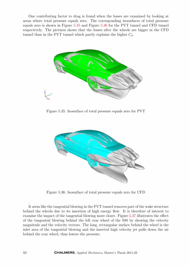
One contributing factor to drag is found when the losses are examined by looking atareas where total pressure equals zero. The corresponding isosurfaces of total pressureequals zero is shown in Figure 5.35 and Figure 5.36 for the PVT tunnel and CFD tunnelrespectively. The pictures shows that the losses after the wheels are bigger in the CFDtunnel than in the PVT tunnel which partly explains the higher Cd.

Figure 5.35: Isosurface of total pressure equals zero for PVT

Figure 5.36: Isosurface of total pressure equals zero for CFD

.It seem like the tangential blowing in the PVT tunnel removes part of the wake structure

behind the wheels due to its insertion of high energy flow. It is therefore of interest toexamine the impact of the tangential blowing more closer. Figure 5.37 illustrates the effectof the tangential blowing behind the left rear wheel of the S80 by showing the velocitymagnitude and the velocity vectors. The long, rectangular surface behind the wheel is theinlet area of the tangential blowing and the inserted high velocity jet pulls down the airbehind the rear wheel, thus lowers the pressure.


Figure 5.37: Velocity contour and vectors behind rear wheel

.The tangential blowing is used to ”fill in” the boundary layer that have started to build

up behind the WDU, with the aim of having a integrated boundary layer displacementthickness of zero at some point downstream of the inlet. However, the velocity vectorsand velocity contour indicates that the tangential blowing acts across a height larger thananticipated, a feat caused by the very high inlet velocity of the jet. In order to investigatethe impact of the tangential blowing on the drag, a new simulation was performed with thetangential blowing turned of. The resulting velocity field and vectors behind the rear canbe seen in Figure 5.38. There is no insertion of high energy flow and the wake behind therear wheel extends all the way down to the floor. Note also that the direction of the flowabove the tangential blowing area is now concentrated to the x-direction, different fromwhen the tangential blowing is activated and the flow is drawn down by the inserted highspeed flow.

Figure 5.38: Velocity contour and vectors behind rear wheel with the tangential blowingdeactivated

.


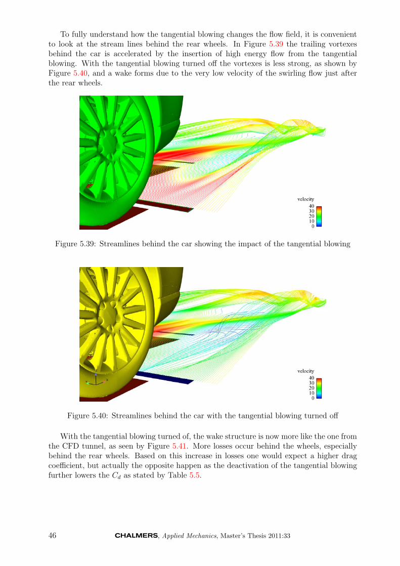
To fully understand how the tangential blowing changes the flow field, it is convenientto look at the stream lines behind the rear wheels. In Figure 5.39 the trailing vortexesbehind the car is accelerated by the insertion of high energy flow from the tangentialblowing. With the tangential blowing turned off the vortexes is less strong, as shown byFigure 5.40, and a wake forms due to the very low velocity of the swirling flow just afterthe rear wheels.

Figure 5.39: Streamlines behind the car showing the impact of the tangential blowing

Figure 5.40: Streamlines behind the car with the tangential blowing turned off

With the tangential blowing turned of, the wake structure is now more like the one fromthe CFD tunnel, as seen by Figure 5.41. More losses occur behind the wheels, especiallybehind the rear wheels. Based on this increase in losses one would expect a higher dragcoefficient, but actually the opposite happen as the deactivation of the tangential blowingfurther lowers the Cd as stated by Table 5.5.


Figure 5.41: Isosurface of total pressure equals zero for PVT with the tangential blowingturned of

Table 5.5: The impact of tangential blowing on drag and lift coefficients for the S80Case Cd Cl

PVT tunnel 0.279 0.135PVT tunnel without tangential blowing 0.272 0.168

This is because even tough the wake structure becomes larger with the tangentialblowing turned of, it is made obsolete by the decrease in stagnation pressure on the frontof the rear wheel, as seen by comparing Figure 5.42 and 5.43, which shows the pressure onthe forward facing part of the car with tangential blowing turned on and off respectively.The larger stagnation pressure on the rear wheels together with the lower pressure behindthe rear wheels when the tangential blowing is activated, contributes to an increase indrag. This behavior is very well matched with observations from experiments in the PVTtunnel.

Figure 5.42: Cp of the forward facing areas of the S80 with tangential blowing turned on


Figure 5.43: Cp of the forward facing areas of the S80 with the tangential blowing turnedoff


The closest experiment possible to compare with the S80 closed front CFD simulationwas the 2007 S80 with the front grill and spoiler opening taped, performed by formerthesis worker James C. Lyon [8]. Even though a taped grill and spoiler means that noair is allowed into the engine bay and cooling package through the front, air can stillenter through the openings of the floor. This means that some differences between theCFD results and the experiments should be expected. Table 5.6 displays the drag and liftcoefficients from the experiment and the CFD calculation. The difference is quite large, abit larger than expected, and has its source in the differences already experienced in theempty tunnel.

Table 5.6: The drag and lift coefficient for the S80 closed front, CFD versus experimentCase Cd Cl

PVT simulation 0.279 0.135Experiment 0.308 0.187

Another hint of the reasons behind the differences between the CFD and experimentis given when comparing the centerline pressure across the S80. The centerline pressure isplotted in Figure 5.44 and there are several disparities found. The pressure is consequentlypredicted higher in the CFD compared to the experiment, regardless of sign. However, careshould be taken when analyzing this figure, since the two cases are different as explainedpreviously in this section. Also, as explained in the subsection Post Processing of thesection Method, the way Cp have been calculated differs and the positions of the pressurepoints have been approximated.


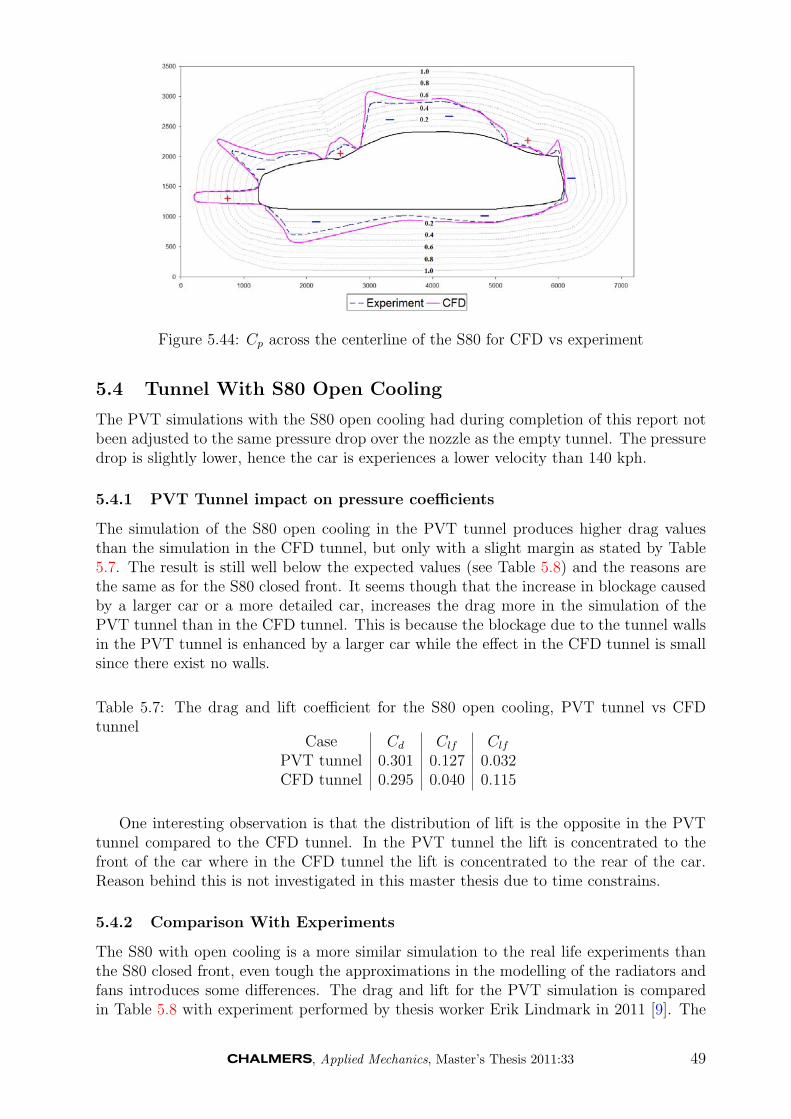
Figure 5.44: Cp across the centerline of the S80 for CFD vs experiment

5.4 Tunnel With S80 Open Cooling

The PVT simulations with the S80 open cooling had during completion of this report notbeen adjusted to the same pressure drop over the nozzle as the empty tunnel. The pressuredrop is slightly lower, hence the car is experiences a lower velocity than 140 kph.


The simulation of the S80 open cooling in the PVT tunnel produces higher drag valuesthan the simulation in the CFD tunnel, but only with a slight margin as stated by Table5.7. The result is still well below the expected values (see Table 5.8) and the reasons arethe same as for the S80 closed front. It seems though that the increase in blockage causedby a larger car or a more detailed car, increases the drag more in the simulation of thePVT tunnel than in the CFD tunnel. This is because the blockage due to the tunnel wallsin the PVT tunnel is enhanced by a larger car while the effect in the CFD tunnel is smallsince there exist no walls.

Table 5.7: The drag and lift coefficient for the S80 open cooling, PVT tunnel vs CFDtunnel

Case Cd Clf Clf

PVT tunnel 0.301 0.127 0.032CFD tunnel 0.295 0.040 0.115

One interesting observation is that the distribution of lift is the opposite in the PVTtunnel compared to the CFD tunnel. In the PVT tunnel the lift is concentrated to thefront of the car where in the CFD tunnel the lift is concentrated to the rear of the car.Reason behind this is not investigated in this master thesis due to time constrains.


The S80 with open cooling is a more similar simulation to the real life experiments thanthe S80 closed front, even tough the approximations in the modelling of the radiators andfans introduces some differences. The drag and lift for the PVT simulation is comparedin Table 5.8 with experiment performed by thesis worker Erik Lindmark in 2011 [9]. The


difference between the calculated Cd compared to the measured Cd is smaller than for theS80 closed front model, 25 drag counts compared to 29 drag counts, but the CFD stillpredicts a lower drag value. The lower lift in the PVT simulation is mainly because of thesimplified floor.

Table 5.8: The drag and lift coefficient for the S80 open cooling, CFD versus experimentCase Cd Cl

PVT simulation 0.301 0.160Experiment 0.326 0.231

In Figure 5.45 Cp across the 2nd slot of both walls for the CFD of the S80 open coolingand the experiment is plotted. The curves follows the same pattern but is of less magnitudein the CFD compared to the experiment. This is a consequence of the large magnitudedifference when the tunnel is empty. The way Cp changes when the S80 is put into thetunnel compared to an empty tunnel is similar in the CFD and experiment. There arestrong reasons to believe that the curve with a car in the tunnel would have been muchmore similar, if the experiment with an empty tunnel had shown a varying pressure of thesame small magnitude as in the CFD (or the other way around).

Figure 5.45: Cp for CFD vs experiment

The experimental measurements in Figure 5.45 is the final proof of the asymmetry ofthe flow in the PVT tunnel.


6 Conclusions

The results have clearly demonstrated that the PVT tunnel has a very unsymmetrical flowfield which have a effect on the results, especially when yawing a car in the tunnel, butalso during tests when the car is positioned in a straight line. The main reason behindthis is the asymmetric support structure of the slotted walls which unfortunately is heavilyincorporated in the core structure of the slotted walls.

The asymmetric behaviour has different effect on the flow field depending on whattype of car is in the tunnel and how unsymmetrical the floor of the car is. A completelysymmetric car, as the S60 model used in this master thesis, is greatly effected since thechoice of side which the approaching air will pass the car on is only dependent on theasymmetry of the support structure. This results in a large inflow on the left side of thecar which creates a very unsymmetrical wake.

When a S80 with a detailed floor is in the tunnel, the flow is not only affected by thewalls but also by the asymmetric floor of the car and the effect from these two suppresseseach other, giving a more symmetric flow than what it is believed to be in reality.

The drag coefficients have consistently been lower in the PVT tunnel compared to thethe experiments but also lower than the CFD tunnel for all simulations except the S80 opencooling. The reason behind this is probably because of the absence of the complete closedair path of the wind tunnel and several details of the geometry in the test section whichif incorporated would have created a less uniform flow, closer to the uniformity measuredin the experiments. The more uniform flow caused by the simplification of the simulatedgeometry gives a less varying pressure across the whole tunnel in the CFD compared to theexperiment, especially for the empty tunnel. This is demonstrated by the Cp plots of theslotted walls which shows large differences when the tunnel is empty but less differenceswhen a car is in the tunnel, a feat which suggests that it is the geometry and not theapproximations in the CFD which is the source.

Reasons behind the general higher drag values of the experiments in the PVT tunnel washard to distinguished since the CFD of the PVT tunnel did not replicate this characteristic,but instead produced the opposite. However, a interesting observation made was that theCd was lowered considerably when the tangential blowing was deactivated. The tangentialblowing could be a contributing factor to the high drag values in the experiments, but thisneeds to be further investigated.


7 Recommendations and Future Work

Since the asymmetry of the walls have showed to be of significant matter, Volvo Carsshould consider modifying the support structure of the slotted walls in order to decreasethe asymmetry of the flow. At least all object and items that are currently placed behindthe slotted walls and which have no important reason for being there, should be removedas they could be influencing the flow.

As the simulations have shown that the flow is a lot more uniform compared to theexperiment, the next step in the simulations should be trying to replicate the inlet flowconditions currently experienced in the PVT tunnel. This can be done by using mea-surements from the tunnel and choosing user defined inlet condition in Fluent. It is alsoimportant to consider implementing a larger part of the wind tunnel, presumably the bendsand turning vanes of the tunnel, which probably have a significant effect on the flow field.The simulation should be concentrated on an empty tunnel since the empty tunnel is thesource of the differences between the PVT simulations and the experiments.

A more thorough study of the PVT tunnel calibration coefficients should be conductedsince they are the basis of important variables such as the pressure coefficient. This is doneby performing several simulations of an empty tunnel with different velocities and thenperforming the regular calibration process for each velocity. New calibration coefficientscan then be calculated and their velocity dependency can be distinguished.

The option of using a complete moving ground, meaning a belt which width extends allthe way to the slotted walls, have been briefly studied during this master thesis. More workshould be carried out regarding this, because using a complete moving ground instead ofthe 5-belt moving ground system and boundary layer control system would greatly simplifythe simulation and remove any uncertainties regarding modeling of the floor.

During this master thesis simulations have been performed with several mesh sizesranging from 30 million cells to above 100 million cells. The calculation expenses havebeen found to be rather cheap, at the longest 15 hours on 180 CPUs for the S80 opencooling which had a cell size of 114 million cells. But the memory demand with increasingmesh size have showed to be a real problem, with Fluent already needing 64 gigabyte worthof RAM to be able to load the 114 million mesh. It is therefore recommended to limit theamount of cells depending of the available memory on the computer used.

The newer versions of Harpoon (4.2a, 4.3a) have showed to be a lot quicker than theolder version 4.1a, especially regarding creation of prism layers where they have beenaround five times quicker. But care should be taken when using version 4.3a as two weekswas lost during this master thesis because of mesh related convergence problems that wassolved by simply using version 4.1a instead.

When using Ensight it is recommended to use scripts and journal files as much aspossible since Ensight can occasionally crash, a feat more frequent when more than onecase have been loaded. It is therefore easier if plots and figures can be produced withoutthe need of opening Ensight.


References

[1] J. Sterneus, T. Walker & T. Bender Upgrade of the Volvo Cars Aerodynamic WindTunnel Technical Paper 2007-01-1043, 2006

[2] Peter Mlinaric Investigation of the Influence of Tyre Deformation and Tyre ContactPatch on CFD Predictions of Aerodynamic Forces on a Passenger Car Master Thesisperformed at Volvo Cars, Chalmers University of Technology 2008

[3] Ansys Fluent User’s Guide Release 12.0, 2009-01-29

[4] H. K. Versteeg & W. Malalasekera An Introduction to Computational Fluid Dynamics,The Finite Volume Method 2nd edition, Pearson Education Limited 2007

[5] Volvo Cars AEDCAE01: Aerodynamic performance assessement of a car exterior withclosed front 2009-09-09

[6] Volvo Cars AEDCAE02: Aerodynamic performance assessement of a car exterior withopen front 2009-09-09

[7] Trevor J. Bender Commissioning Report: PVT Ground Simulation Upgrade InternalTechnical Report at Volvo Car Corporation 2006

[8] James C. Lyon Automobile Aerodynamics on the Road and in the Wind Tunnel - ACorrelation Study Master thesis performed at Volvo Cars, KTH, 2008

[9] Erik Lindmark Analysis of Pressure Measurements in PVT Compared to Hallered andCFD Master thesis performed at Volvo Cars, Linkopings Universitet, 2011

[10] Mattias Eng Investigation of Aerodynamic correction methods applied to a slotted wallWind Tunnel Master Thesis performed at Volvo Cars, Technische Universitat Berlin,2009

[11] Stephane Cyr, Kang-Duck Ih & Sang-Hyun Park Accurate Reproduction of Wind-Tunnel Results with CFD Technical Paper 2011-01-0158, 2011

[12] R. H. Barnard Road Vehicle Aerodynamic Design, An Introduction 2nd edition, Me-shaero Publishing 2001

[13] S. Perzon On Blockage Effects in Wind Tunnels - A CFD study Technical Paper2001-01-0705, 2001

[14] O. Fischer, T. Kuthada, N. Widdecke & J. Wiedemann CFD Investigations of WindTunnel Interference Effects Technical Paper 2007-01-1045, 2007


Documents

CFDSimulationoftheVolvoCarsSlottedWalls Wind …publications.lib.chalmers.se/records/fulltext/143242.pdfCFDSimulationoftheVolvoCarsSlottedWalls Wind Tunnel Master’sThesisinSolidandFluidMechanics