Embed Size (px)
Citation preview
Department of Civil and Environmental Engineering Division of Structural Engineering Concrete Structures Research Group CHALMERS UNIVERSITY OF TECHNOLOGY Gothenburg, Sweden 2016 Master’s Thesis BOMX02-16-138
Assessment of simulation codes for offshore wind turbine foundations Master’s Thesis in the Master’s Programme Structural Engineering and Building Technology
ÖMER FARUK HALICI
HILLARY MUTUNGI
Replace the shaded box with a picture
illustrating the content of the thesis.
This picture should be “floating over the
text” in order not to change the position
of the title below (right clic on the
picture choose “Layout” and “In front of
text”
Instructions for use of this template
Start saving the template file as your word-file (docx). Replace the text in the text
boxes on the first page, also in the footer. Replace only the text inside the text boxes.
The text box is visible when you click on the text in it. Update all linked fields in the
rest of the document by choosing “Select All” (from the Home tool bar) and then
click the F9-button. (The footers on page III and IV need to be opened and updated
separately. Click in the text box in the footer and update with the F9-button.) Insert
text in some more text boxes on the following pages according to the instructions in
the comments. Write your thesis using the formats (in detail) and according to the
instructions in this template. When it is completed, update the table of contents. The
thesis is intended to be printed double-sided.
To edit footer choose “Footer” from the
Insert tool bar and then choose “Edit
footer”. After editing choose “Close
header and footer”.


MASTER’S THESIS BOMX02-16-138
Assessment of simulation codes for offshore wind turbine
foundations
Master’s Thesis in the Master’s Programme Structural Engineering and Building Technology
ÖMER FARUK HALICI
HILLARY MUTUNGI
Department of Civil and Environmental Engineering
Division of Structural Engineering
Concrete Structures Research Group
CHALMERS UNIVERSITY OF TECHNOLOGY
Gothenburg, Sweden 2016


Assessment of simulation codes for offshore wind turbine foundations
Master’s Thesis in the Master’s Programme Structural Engineering and Building
Technology
ÖMER FARUK HALICI
HILLARY MUTUNGI
© ÖMER FARUK HALICI, HILLARY MUTUNGI 2016
Examensarbete BOMX02-16-138/ Institutionen för bygg- och miljöteknik,
Chalmers tekniska högskola 2016
Department of Civil and Environmental Engineering
Division of Structural Engineering
Concrete Structures Research Group
Chalmers University of Technology
SE-412 96 Göteborg
Sweden
Telephone: + 46 (0)31-772 1000
Cover:
Figure shows the wind turbines located at Middelgrunden, 2 km off shore east of
Copenhagen, Denmark (Bertrand, 2002)
Department of Civil and Environmental Engineering, Gothenburg, Sweden, 2016

CHALMERS, Civil and Environmental Engineering, Master’s Thesis BOMX02-16-138
I
Assessment of simulation codes for offshore wind turbine foundations
Master’s thesis in the Master’s Programme Structural Engineering and Building
Technology
ÖMER FARUK HALICI
HILLARY MUTUNGI
Department of Civil and Environmental Engineering
Division of Structural Engineering
Concrete Structures Research Group
Chalmers University of Technology
ABSTRACT
Offshore wind energy has the potential to become a leading renewable energy source.
However, the cost of offshore wind turbine foundations is a major obstacle to the
breakthrough of offshore wind energy development. There are a number of simulation
codes that describe aerodynamic, hydrodynamic and serviceability response of
offshore wind turbines. Nonetheless, each of these codes has its own limitations and
capabilities in terms of; foundation type, environmental loading conditions as well as
general modelling assumptions. Most simulation codes currently used in practice are
limited to simple towers with monopile or gravity base foundations. However, they
are being extended to model more developed foundation types, including tripods,
jackets etc. Therefore, it is important to assess and judge the applicability of these
codes to model such developed structures, which forms the purpose for this thesis.
To assess the capabilities and limitations of the studied simulation codes, principles
and theories used were established. A classification of the codes was then made
according to the observed principles. After that, three simulation codes (FASTv8,
FOCUS6 and ASHES) were selected and examined through case studies with
different types of foundations and loading conditions in order to study the codes
practically. As expected, the results showed a variety of differences and similarities.
In addition, some codes were more functional than others. For instance, in terms of
the ability to describe loads with more advanced models, ability to create design load
combinations etc.
In conclusion, it was confirmed that prior to choosing the appropriate simulation code
for a given design, one has to consider the ability to describe the environmental
conditions that the structure will face during its service life and the appropriate
background required for the code to model the foundation.
Key words: Offshore wind energy, Simulation codes, Wind turbine, Foundations

CHALMERS, Civil and Environmental Engineering, Master’s Thesis BOMX02-16-138
II

CHALMERS, Civil and Environmental Engineering, Master’s Thesis BOMX02-16-138 III
Contents
ABSTRACT I
CONTENTS III
PREFACE VII
NOTATIONS VIII
1 INTRODUCTION 1
1.1 Background and project description 1
1.2 Purpose and objectives 1
1.3 Scope 1
1.4 Method 2
2 DESCRIPTION OF OFFSHORE WIND TURBINE 4
2.1 Offshore wind turbine foundation 4
2.2 Offshore wind turbine tower 4
2.3 Loads acting on OWT 5 2.3.1 Wind 5
2.3.2 Waves 5
2.3.3 Currents 6 2.3.4 Seismic loads 6 2.3.5 Ice loads 6
2.3.6 Dead loads 7 2.3.7 Accidental loads 7
2.3.8 Further design consideration 7
2.4 Dynamic nature of an OWT 8
3 OFFSHORE WIND TURBINE FOUNDATIONS 10
3.1 Monopiles 10
3.2 Jacket structures 11
3.3 Gravity based structures 11
3.4 Tripod structures 12
3.5 Floating structures 13
4 PRINCIPLES USED IN OWT SIMULATION CODES 14
4.1 Soil interaction modelling 14 4.1.1 Coupled spring model 14
4.1.2 Distributed springs model 14 4.1.3 Effective /Apparent fixity model 15
4.2 Wind modelling and aerodynamic loads 15
4.2.1 Stochastic wind profiles 15

CHALMERS, Civil and Environmental Engineering, Master’s Thesis BOMX02-16-138 IV
4.2.2 Aerodynamic loads 17
4.3 Wave modelling and hydrodynamic loads 19 4.3.1 Deterministic wave models 19 4.3.2 Stochastic wave models 21
4.3.3 Hydrodynamic loads 24
4.4 Currents 25
4.5 Analysis methods 26
4.6 Analysis techniques 27 4.6.1 Sequential approach technique 27
4.6.2 Semi-coupled approach technique 28 4.6.3 Fully coupled approach technique 28
5 SIMULATION CODES AND CLASSIFICATION 30
5.1 Current simulation codes in use 30 5.1.1 FAST (Fatigue, Aerodynamics, Structures and Turbulence) 30 5.1.2 Flex5 31
5.1.3 Bladed 32 5.1.4 ADCoS 33 5.1.5 ADAMS/WT & AeroDyn 35
5.1.6 HAWC2 36 5.1.7 ASHES 37
5.1.8 TURBU Offshore 38
5.1.9 FOCUS6 39
5.1.10 OneWind 41 5.1.11 USFOS-vpOne 42
5.1.12 SESAM 43
5.2 Comparison of codes 45
6 OWT DESIGN PROCESS 47
6.1 Design Environment loads 47 6.1.1 Wind loads 47
6.1.2 Wave loads 47 6.1.3 Wind generated waves 48
6.1.4 Wind generated current 48
6.2 Design input data for the codes 49 6.2.1 Geometry and material properties. 49 6.2.2 Aerodynamic data 49 6.2.3 Hydrodynamic data 49
6.2.4 Initial and boundary conditions 50 6.2.5 Soil interaction data 50 6.2.6 Computational specifications 50 6.2.7 Summary 50
7 CASE STUDY AND CODE COMPARISON 52
7.1 Pre-study 52

CHALMERS, Civil and Environmental Engineering, Master’s Thesis BOMX02-16-138 V
7.1.1 Pre-Study with OC4 Load Case 2.1 52 7.1.2 Pre-Study with OC4 Load Case 2.3a 53 7.1.3 Special case of OC4 Load Case 2.3a 54
7.2 RNA and tower definitions used in the studies 56
7.2.1 NREL 5MW Wind turbine model 56 7.2.2 Tower 57
7.3 Definition of load cases 57 7.3.1 Environmental effects measured from the site. 59
7.4 Comparison study for tripod structure 60
7.4.1 Description of the structure 60 7.4.2 Modelling the support structure 62
7.4.3 Foundation model 62 7.4.4 Results 62
7.5 Comparison study for the gravity base structure 71 7.5.1 Description of the structure 71 7.5.2 Modelling the support structure 73
7.5.3 Foundation model 73 7.5.4 Results 73
8 DISCUSSION 82
8.1 Comparison of the simulation codes 82
8.2 Discussion of the results from a design vantage point 84
9 CONCLUSION AND FUTURE RECOMMENDATIONS 86
9.1 Conclusion 86
9.2 Future recommendations 87
10 REFERENCES 88
11 APPENDICES 92
11.1 Appendix 1 – Matlab code for gravity base model 92
11.2 Appendix 2 – Fast input data for tripod structure model for load case 6 97

CHALMERS, Civil and Environmental Engineering, Master’s Thesis BOMX02-16-138 VI

CHALMERS, Civil and Environmental Engineering, Master’s Thesis BOMX02-16-138 VII
Preface
In this project, classification and assessment of offshore wind turbine simulation
codes have been made based on literature and case studies. In the classification study,
several simulation codes were studied and adopted theories and principles were
outlined. The case studies though, included only three of these simulation codes
namely, FASTv8 (NREL), FOCUS6 (WMC) and ASHES (SIMIS). Moreover, a
jacket, a tripod and a gravity base foundation models were created in these codes and
studied in detail with specific load cases. The results were then used to assess and
establish the limitations and capabilities of these simulation codes in relation to
modelling such structures. This thesis is part of an ongoing research project named
ISEAWIND financed by Swedish Energy Agency and NCC. The project was carried
out at the Department of Structural Engineering, Concrete Structures Research Group.
The project has been carried out with Alexandre Mathern as the supervisor and Dr.
Rasmus Rempling as the main supervisor and examiner. We would like to thank them
for their devoted assistance and guidance throughout this project. In addition, we
would like to thank Dr. Jason Jonkman of NREL, Dr. Paul E. Thomassen of SIMIS
and the support team of WMC for their valuable contributions and technical advice.
Gothenburg, June 2016
Ömer Faruk Halici & Hillary Mutungi

CHALMERS, Civil and Environmental Engineering, Master’s Thesis BOMX02-16-138 VIII
Notations
Roman upper case letters
DC Variable notation for the drag coefficient
LC Variable notation for the lift coefficient
MC Variable notation for the inertia coefficient
D Variable notation for the diameter of the structure
F Variable notation for the fetch
LK Notation for spring lateral stiffness
RK Notation for spring rocking stiffness
VK Notation for spring vertical stiffness
VLK
Notation for spring cross-coupling stiffness
UL
Variable notation for the length scale of the wind speed
vL
Variable notation for the integral length scale
( )uS f
Variable notation for spectral density function
( )S
Variable for the wind wave function
( )U H
Variable for the 10-minute wind speed at a height H
( )U z
Variable for the 10-minute wind speed at a height z
0U
Variable notation for the 1-hour mean wind speed at 10m height
1/3U
Variable notation for the velocity of the wave at the significant wave
height
10U
Variable notation for the 10-minute mean wind speed
0z
Notation for the ground roughness parameter
V Variable notation for the absolute velocity
wV
Variable notation for mean wind speed
Roman lower case letters
a Variable notation for the induction factor

CHALMERS, Civil and Environmental Engineering, Master’s Thesis BOMX02-16-138 IX
f Variable notation for the frequency
tf Variable notation for the total wave load on a structure
Df Variable notation for the drag load on a structure due to waves
Mf Variable notation for the inertia load on a structure due to waves
g Notation for the gravitation acceleration
r Variable notation for element radius
u Variable Notation for the horizontal wave particle velocity
cu
Variable Notation for the velocity of a current
u Variable Notation for the horizontal wave particle acceleration
0wind Variable notation for the wind generated current velocity
Greek upper case letters
Variable notation for the blade rotational speed
Greek lower case letters
Notation for the constant that relates the wind speed and fetch length
Variable notation for the flow angle to the blade
Variable notation for the peak factor
r Variable notation for tip speed ratio
c Variable notation for the direction of a current
Variable notation for air density
Variable notation for local solidity
' Variable notation for local solidity
U Variable notation for the standard deviation of the wind speed
0 Variable notation for modal angular frequency
Variable notation angular frequency
p
Variable notation for peak angular frequency

CHALMERS, Civil and Environmental Engineering, Master’s Thesis BOMX02-16-138 X
CHALMERS, Civil and Environmental Engineering, Master’s Thesis BOMX02-16-138 1
1 Introduction
1.1 Background and project description
An offshore wind turbine is a power production unit having a large vanned wheel
rotated by the wind, situated at a considerable distance from the sea shore to capture
stronger winds. In this context, an offshore wind turbine (OWT) refers to the entire
assembly of the wind turbine including the rotor nacelle assembly (RNA) and its
support structure (tower and foundation). Offshore wind energy has a large potential
to become a serious part of renewable energy sources in the near future. However, the
main obstacle to building an offshore wind turbine is being relatively low cost
efficient which is mainly generated from the high expenditure of foundations. Apart
from that, the improvement of OWT foundation design is not an easy task due to
complicated loading cases that these structures are exposed to (wind loads, wave
loads, ice and currents)
Today there exists a number of advanced simulation codes to model OWTs and their
foundations, however, each code has its own limitations as being suitable for a
specific type of foundations and/or loading conditions. Moreover, there exists various
necessary input data for each code and different assumptions that the model is based
on. It is important to note though, that the term “simulation code” as used in this
thesis refers to a computer program. This should not be misunderstood for the term
“design code”, which refers to a documented standard of practice.
Most of the simulation codes currently used in practice were until recently limited to
simple towers with monopile or gravity base foundations. However, they are extended
to meet the requirements of modelling more developed support structures like tripods,
jackets and to some extent, floating structures. It is therefore important to judge the
accuracy, suitability and capability of these codes based on a detailed study of their
application.
This master’s thesis is part of a research project named ISEAWIND that is financed
by the Swedish Energy Agency and NCC.
1.2 Purpose and objectives
The main purpose of this thesis project was to study and assess the codes currently
used in practical OWT simulation and design, particularly foundations.
The objectives of the thesis were as follows;
- Literature study of the currently used OWT simulation codes.
- Classification of the OWT simulation codes.
- Assessing suitable codes by using them on case studies of different foundation
forms for OWT.
- Describing the limitations and capabilities of these simulation codes.
1.3 Scope
Although an OWT refers to the entire wind turbine structure, the scope of this thesis
was limited to aspects relevant to the foundation and its design. In addition, the case

CHALMERS, Civil and Environmental Engineering, Master’s Thesis BOMX02-16-138 2
studies were based only on the NREL offshore 5-MW baseline OWT as discussed in
Section 7.2.1.
The case study in this thesis investigated three types of OWT support structures
namely; jacket structure, symmetric tripod structure and gravity base structure. The
jacket structure was used in the pre-study of the simulation codes (see Section 7.1).
The tripod and the gravity base structures where studied according to real
environmental conditions measured at Blekinge offshore site. The foundation type
used was the fixed type whereby the flexible aspects of the soil were disregarded.
Models of these support structures were studied and tested using only three simulation
codes i.e. FAST v8 developed by the National Renewable Energy Laboratory (USA),
ASHES 2.3.1 developed by SIMIS (Norway) and FOCUS6 developed by WMC
(Netherlands). The reasons for limiting the study to only these three codes were
mainly due to the timeline of the project, the availability of the code licence as well as
technical support from the code developers. All information about the rest of the
codes discussed in Section 5.1 is based solely on written documentation about the
codes.
Although API (2007) and DNV-OS-J101 (2014) specify more loads against which an
OWT should be designed, this project was limited to only such environmental loads
as waves, wind and currents. In just a few instances, the gravity load was considered
but solely for model verification purposes.
1.4 Method
The first task of this thesis was to investigate the state-of-the-art simulation codes
existing for OWT foundations. This involved studying a vast amount of literature and
searching for the codes and software that are currently used to design. The logic
behind the codes was investigated to understand the necessary input data and different
assumptions on which OWT models are based.
Following the literature study, the second task was to make a classification of the
simulation codes. It was then possible to understand which kind of design the code
applies to, for instance, the type of structure and underlying design principles on
which the code is based.
The third task was to assess the codes by applying them on case studies with certain
types of turbine foundations in order to make comprehensive code-to-code and code-
to-real data comparisons. This provided a deeper understanding of simulation codes
and made it possible to analyse the accuracy of the results and capabilities of codes. It
was not possible to access actual turbine data and instead, previous project results
were used. One such project was the OC4 project (Vorpahl et al., 2011) and indeed
this provided the basis for the code pre-study task. In the pre-study, the codes were
used to model the exact support structure and load cases studied in the OC4 project to
ensure that similar results were obtained. The sole reason for this exercise was to
ensure familiarity with these codes before taking on other support structures.

CHALMERS, Civil and Environmental Engineering, Master’s Thesis BOMX02-16-138 3
Following the pre-study, a symmetric tripod and a gravity base foundation was
modelled in FASTv8 (NREL), FOCUS6 (WMC) and ASHES (SIMIS) with a variety
of load cases to inspect the limitations and capabilities of the simulation codes.
Supervisory meetings as well as discussions with the technical support teams from the
code developers were used as a means to ensure that the modelling procedure was
done correctly. In addition, the analysis results were constantly reviewed to validate
that the output was consistent. While the pre-study was done on dummy
environmental load conditions adopted from the OC4 project, the case study featured
actual environmental load conditions from Blekinge offshore site in South-Eastern
Sweden. This provided grounds to simulate how such OWT support structures would
behave if they were actually constructed.
Finally, with sufficient information, the limitations and capabilities of each code were
established based on such criteria as: type of foundation that the code can be applied,
the methodologies and design principles of codes as well as the ability to define and
handle different types of loads.

CHALMERS, Civil and Environmental Engineering, Master’s Thesis BOMX02-16-138 4
2 Description of offshore wind turbine
In this chapter, primary components of offshore wind turbines and the fundamental
design principles will be discussed. Passon and Kühn define the support structure of
an OWT as consisting of the whole structure below the yaw system (2005). Moreover,
it is convenient to separate the support structure into distinct parts or modules for the
purpose of modelling and conceptual disposition (Ibid.). In the context of this study,
the OWT support structure is divided into the tower and the foundation. A detailed
discussion of these components, their dynamic nature, as well as the loads that affect
them follows in Section 2.1 to 2.4.
2.1 Offshore wind turbine foundation
A foundation is the main component that supports the OWT structure against
horizontal and vertical loads. As Kaiser and Snyder mentioned, there exists various
types of foundations that can be applied to different environmental properties of an
OWT structure such as, water depth, wind speed, wave heights and weight of the
turbine (2012). In order to meet today’s high energy demand and catch greater wind
potential, OWTs need to be placed further away from the shore in deeper waters.
However, it is apparent that hydrodynamic and aerodynamic loads increase as the
water depth and distance from the shore increases.
Foundation selection plays an important role in the design of offshore wind farms,
since there are large financial implications that accompany the choice of the
foundation. Typically the foundation costs 25% to 34% of the overall cost of building
an OWT (Bhattacharya 2014). In addition to the financial viability of the project, the
nature of the loads acting on OWTs means that the foundation forms a critical
component of the OWT structure, as will be seen later.
Foundations for OWTs can be classified into two main types; the fixed types and
floating types. The fixed type foundations are only effective in relatively shallow
waters (<60m), whereas the floating type foundations are developed for deeper waters
(>60m). As Passon and Kühn (2005) pointed, OWT structures can be grouped into the
first, second and third generation. The first generation includes fixed foundations such
as mono-pile and gravity base foundations. These are effective in shallow waters less
than 30m deep. The second generation covers a more sophisticated range of
foundations such as tetrapod caisson, asymmetric-tripod caisson, jacketed caisson,
tripod caisson and tripod pile foundations. These are effective even in deeper waters,
but still limited to 60m (Bhattacharya 2014). The third generation is the floating type.
It is by all means the most cost effective solution in deep waters and has no limit to
which water depth it can be installed.
2.2 Offshore wind turbine tower
The tower is considered as part of the turbine support structure that resides above the
foundation. According to Jonkman et al. (2009), the tower properties will depend on
the type of foundation used to carry the RNA. The type of foundation will in turn
depend on the site conditions. The properties of the site vary significantly in terms of
water depth, soil type, and wind and wave severity.
CHALMERS, Civil and Environmental Engineering, Master’s Thesis BOMX02-16-138 5
A tower structure can be a mono-tower or a jacket. In addition, a variety of tower and
foundation combinations can be made depending on the design requirements.
2.3 Loads acting on OWT
The loads acting on an OWT structure can be grouped into static or dynamic loads.
Static loads relate mainly to the self-weight of the components. A case of static loads
due to the environment is ice on the structure. Dynamic loads relate mainly to the
environment in the form of wind or water interaction, and thus classified as
aerodynamic and hydrodynamic respectively.
As Bhattacharya (2014) states, the most challenging of these load classes are the
dynamic loads. Moreover, Van Der Tempel et al. (2011) add that for OWTs, the
assessment of environmental parameters is more extensive than for land turbines. On
land, turbines can be designed following a class prescribing the wind regime and the
required resilience of the turbine itself. However for OWTs, the winds are less
turbulent but more formidable. In addition, the offshore environment features other
actions due to the water waves and currents. This implies that an engineer designing
an OWT faces a more daunting challenge and must fully understand the behaviour
and magnitude of the dynamic loads before proceeding with the design. In this
section, the loads will be discussed in detail.
Other loads that affect offshore structures in general include; earthquakes, accidental
loads, fire and blast loading. (API RP 27, cited in Bai and Jin 2016).
2.3.1 Wind
Field experiments have shown that the distributed wind velocity is variable in space,
time and direction (Molenaar, cited in Van Der Tempel et al. 2011). It is rather
complicated though to consider the effect of variation of wind velocity in more than
one direction. For simplicity, wind is only considered in the horizontal (frontal)
direction. This assumption reduces the complexity of the wind model such that it only
varies with height and time (see Figure 2.1).
Wind is a significant design factor. The wind conditions used in design should be
determined from appropriate and detailed wind data statistics for a specific site. In
addition, this data should be consistent with other associated environmental
parameters (Bai and Jin 2016).
2.3.2 Waves
Sea waves result from wind blowing across the surface of the water and they form one
of the major components of environmental forces affecting OWTs. These often start
as minute ripples and can grow considerably with time. As the waves crush against
the OWT foundation, they cause considerable action whose magnitude depends on the
wave height and wave period. Waves are random, varying in height and length and as
Bai and Jin state; they can approach an OWT from more than one direction
simultaneously (2016). Due to this random nature, the sea state is usually described in
terms of statistical wave parameters such as significant wave length, spectral peak
period, spectral shape, and directionality.
CHALMERS, Civil and Environmental Engineering, Master’s Thesis BOMX02-16-138 6
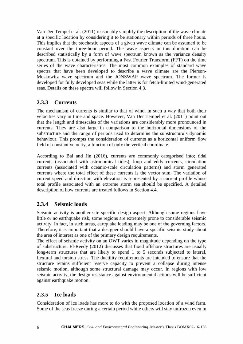
Van Der Tempel et al. (2011) reasonably simplify the description of the wave climate
at a specific location by considering it to be stationary within periods of three hours.
This implies that the stochastic aspects of a given wave climate can be assumed to be
constant over the three-hour period. The wave aspects in this duration can be
described statistically by a form of wave spectrum known as the variance density
spectrum. This is obtained by performing a Fast Fourier Transform (FFT) on the time
series of the wave characteristics. The most common examples of standard wave
spectra that have been developed to describe a wave climate are the Pierson-
Moskowitz wave spectrum and the JONSWAP wave spectrum. The former is
developed for fully developed seas while the latter is for fetch-limited wind-generated
seas. Details on these spectra will follow in Section 4.3.
2.3.3 Currents
The mechanism of currents is similar to that of wind, in such a way that both their
velocities vary in time and space. However, Van Der Tempel et al. (2011) point out
that the length and timescales of the variations are considerably more pronounced in
currents. They are also large in comparison to the horizontal dimensions of the
substructure and the range of periods used to determine the substructure’s dynamic
behaviour. This prompts the consideration of currents as a horizontal uniform flow
field of constant velocity, a function of only the vertical coordinate.
According to Bai and Jin (2016), currents are commonly categorised into; tidal
currents (associated with astronomical tides), loop and eddy currents, circulation
currents (associated with oceanic-scale circulation patterns) and storm generated
currents where the total effect of these currents is the vector sum. The variation of
current speed and direction with elevation is represented by a current profile whose
total profile associated with an extreme storm sea should be specified. A detailed
description of how currents are treated follows in Section 4.4.
2.3.4 Seismic loads
Seismic activity is another site specific design aspect. Although some regions have
little or no earthquake risk, some regions are extremely prone to considerable seismic
activity. In fact, in such areas, eartquake loading may be one of the governing factors.
Therefore, it is important that a designer should have a specific seismic study about
the area of interest as one of the primary design requirements.
The effect of seismic activity on an OWT varies in magnitude depending on the type
of substructure. El-Reedy (2012) discusses that fixed offshore structures are usually
long-term structures that are likely to spend 1 to 5 seconds subjected to lateral,
flexural and torsion stress. The ductility requirements are intended to ensure that the
structure retains sufficient reserve capacity to prevent a collapse during intense
seismic motion, although some structural damage may occur. In regions with low
seismic activity, the design resistance against environmental actions will be sufficient
against earthquake motion.
2.3.5 Ice loads
Consideration of ice loads has more to do with the proposed location of a wind farm.
Some of the seas freeze during a certain period while others will stay unfrozen even in

CHALMERS, Civil and Environmental Engineering, Master’s Thesis BOMX02-16-138 7
sub-zero temperatures. A typical example of a sea which does not often freeze is the
North Sea, while the Baltic Sea often freezes during winter. The freezing of the water
obviously creates a challenge for all possible exploration efforts. To imagine the
effect of ice on an OWT substructure, it is important to understand the drifting of ice
in a sea. El-Reedy (2012) reports that, drifting ice travels at a speed of 1-7% of the
speed of the wind, of course depending on the mass of ice lump. The bigger the ice
mass, the more momentum it will have. Consequently, the more impact it will have on
an OWT structure.
El-Reedy (2012) adds that the effect of ice load depends on the spacing of individual
members, and generally the following rules will apply;
1- Spacing ≥ 6 times the substructure element diameter; Ice is idealised to crush
against the tubular members and pass through and around the platform. For
groups of tubular members of different sizes, the average tubular diameter can
be used to determine the spacing.
2- Spacing ≤ 4 times the substructure element diameter; with decreased spacing
between substructure legs, ice blocks can wedge inside the structure and the
contact area becomes the out to out dimension across the closely spaced
members in the direction of the ice movement.
3- 4 ≤ Spacing ≤ 6 times the substructure diameter; linear interpolation takes
effect.
It is worth noting that the frost and ice which may build up as gravity load on the
turbine blades is often not considered since it is accounted for in the blade design.
2.3.6 Dead loads
As briefly explained earlier, the dead load is the total weight of each individual
component that makes up the entire OWT. The certainty of this category of loads
makes them relatively simple to deal with in design since the density of the materials
used to set up the structure is known as well as the weight of the elements of the
RNA.
2.3.7 Accidental loads
Due to the situation of an OWT, the occurrence of accidental loads is something of
low probability. However, it is worth noting that ship collusions must be taken into
consideration in the design.
2.3.8 Further design consideration
In addition to the loads discussed, it is important to consider the effect of marine
growth as well as scour. Marine growth increases the diameter of a jacket or pile
member and thereby enhances the drag force from currents and waves. Consideration
of marine growth is as much a site specific aspect as scour prediction. For further
reading, the reader is referred to API 1.5 cited in El-Reedy (2012).
CHALMERS, Civil and Environmental Engineering, Master’s Thesis BOMX02-16-138 8
2.4 Dynamic nature of an OWT
OWTs are dynamically sensitive structures because of their shape and form. The
eigenfrequencies of these slender structures are very close to the excitation
frequencies imposed by the environment and mechanical loads. Therefore, in order to
avoid resonance, it requires a fundamental knowledge of structural response and
precise calculations.
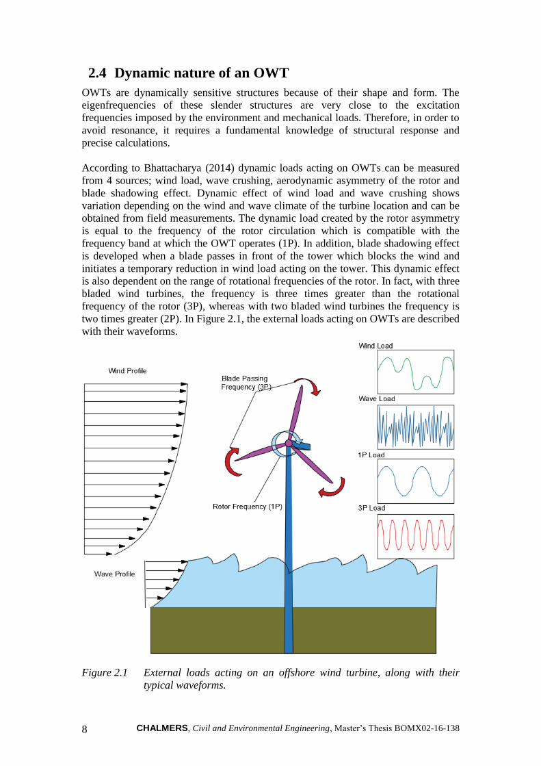
According to Bhattacharya (2014) dynamic loads acting on OWTs can be measured
from 4 sources; wind load, wave crushing, aerodynamic asymmetry of the rotor and
blade shadowing effect. Dynamic effect of wind load and wave crushing shows
variation depending on the wind and wave climate of the turbine location and can be
obtained from field measurements. The dynamic load created by the rotor asymmetry
is equal to the frequency of the rotor circulation which is compatible with the
frequency band at which the OWT operates (1P). In addition, blade shadowing effect
is developed when a blade passes in front of the tower which blocks the wind and
initiates a temporary reduction in wind load acting on the tower. This dynamic effect
is also dependent on the range of rotational frequencies of the rotor. In fact, with three
bladed wind turbines, the frequency is three times greater than the rotational
frequency of the rotor (3P), whereas with two bladed wind turbines the frequency is
two times greater (2P). In Figure 2.1, the external loads acting on OWTs are described
with their waveforms.
Figure 2.1 External loads acting on an offshore wind turbine, along with their
typical waveforms.
CHALMERS, Civil and Environmental Engineering, Master’s Thesis BOMX02-16-138 9
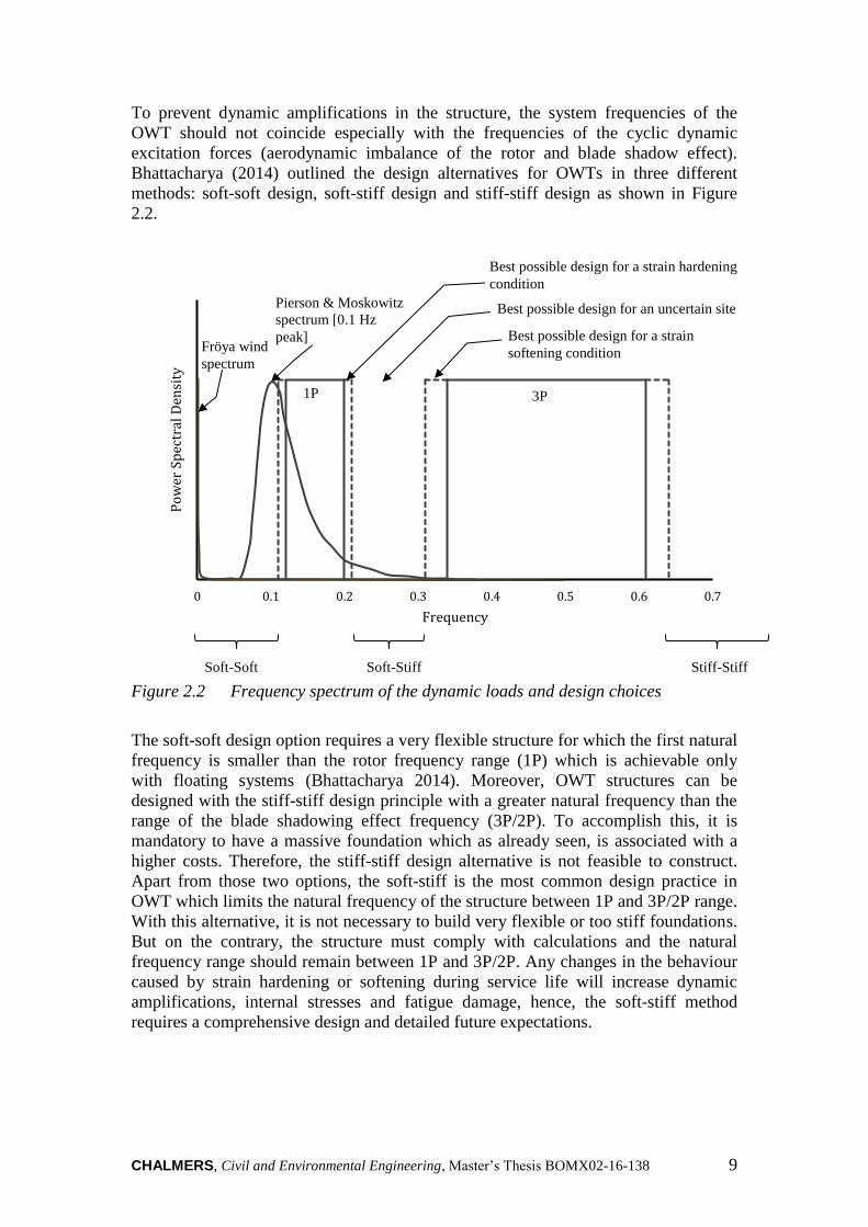
To prevent dynamic amplifications in the structure, the system frequencies of the
OWT should not coincide especially with the frequencies of the cyclic dynamic
excitation forces (aerodynamic imbalance of the rotor and blade shadow effect).
Bhattacharya (2014) outlined the design alternatives for OWTs in three different
methods: soft-soft design, soft-stiff design and stiff-stiff design as shown in Figure
2.2.
Figure 2.2 Frequency spectrum of the dynamic loads and design choices
The soft-soft design option requires a very flexible structure for which the first natural
frequency is smaller than the rotor frequency range (1P) which is achievable only
with floating systems (Bhattacharya 2014). Moreover, OWT structures can be
designed with the stiff-stiff design principle with a greater natural frequency than the
range of the blade shadowing effect frequency (3P/2P). To accomplish this, it is
mandatory to have a massive foundation which as already seen, is associated with a
higher costs. Therefore, the stiff-stiff design alternative is not feasible to construct.
Apart from those two options, the soft-stiff is the most common design practice in
OWT which limits the natural frequency of the structure between 1P and 3P/2P range.
With this alternative, it is not necessary to build very flexible or too stiff foundations.
But on the contrary, the structure must comply with calculations and the natural
frequency range should remain between 1P and 3P/2P. Any changes in the behaviour
caused by strain hardening or softening during service life will increase dynamic
amplifications, internal stresses and fatigue damage, hence, the soft-stiff method
requires a comprehensive design and detailed future expectations.
0 0.1 0.2 0.3 0.4 0.5 0.6 0.7
Po
wer
Sp
ectr
al D
ensi
ty
Frequency
3P
Best possible design for a strain
softening condition
1P
Fröya wind
spectrum
Best possible design for an uncertain site
Best possible design for a strain hardening
condition
Soft-Soft Soft-Stiff Stiff-Stiff
Pierson & Moskowitz
spectrum [0.1 Hz
peak]

CHALMERS, Civil and Environmental Engineering, Master’s Thesis BOMX02-16-138 10
3 Offshore Wind Turbine Foundations
3.1 Monopiles
As mentioned in the introduction, monopiles are the most common foundation
alternative for OWT structures. They consist of a pile and a transition piece (see
Figure 3.1) which offers a relatively simple design and cheap support solution. A
monopile is a thick walled steel pipe with a large diameter from 4 to 6 meters which
can either be driven/hammered into the seabed or be grouted into drilled rock. The
general practice is inserting the 40-50% of the pile into the seabed, depending on
water depth, soil type, design load, etc. (Kaiser and Snyder 2012). It is also possible to
use suction caissons for anchoring a monopile in tough soil conditions were
driving/hammering is hard and expensive. In some cases, monopiles can be
fastened/guyed using cables anchored to the seabed so as to increase the stiffness of
the structure.
Figure 3.1 Monopile foundation (4C Offshore LTD 2016)
Monopile foundations are feasible up to 30 meters of water depth, but due to its
simplicity, there is a big trend to build it in deeper waters. However, increasing
diameter and length bring other challenges including buckling problems, limited
information in design codes, installation issues and cost (Bhattacharya 2014). On the
other hand, considering current developments in design and the fact that not all
shallow waters with great wind potential have been utilized yet by wind power, one
can say that monopile foundations will still be a good option in foundation design in
near future.

CHALMERS, Civil and Environmental Engineering, Master’s Thesis BOMX02-16-138 11
3.2 Jacket structures
The foundation can be built with a truss system (jacket) of steel tubular elements that
can be placed on caissons, piles and gravity based platforms to provide required
stiffness to OWT structures. A jacket structure is a good alternative to monopile
foundations in deeper waters. It can be built with a 3-leg or a 4-leg configuration
depending on environmental conditions at the site. Kaiser and Snyder (2012) claim
that since jacket structures are heavy and require expensive transportation equipment,
they are preferred usually in deeper waters (>50m). Today’s trend is building OWTs
in shallow waters to reduce the cost, therefore, jacket structures are not selected often.
Figure 3.2 (Crampsie 2014) captures a jacket structure that is already built.
Figure 3.2 Jacket structure (Crampsie 2014)
3.3 Gravity based structures
Gravity based foundations are basically concrete shell structures that transfer vertical
loads to the ground and resist horizontal (wave, wind, etc.) loads by their own gravity.
These structures are usually preferred in sites where driving a pile is tough and
expensive. Although constructing a gravity based foundation is less expensive than
building a monopile, this method requires ground improvement and capability of
handling massive concrete blocks onshore and offshore. There is also a need for a
shipyard near the wind farm from where the massive structures can be floated,
dragged to the wind farm yard and sunk (Malhotra 2010). Figure 3.3 (Kaiser and
Snyder 2012) shows gravity base foundations under construction.

CHALMERS, Civil and Environmental Engineering, Master’s Thesis BOMX02-16-138 12
Figure 3.3 Gravity base foundations (Kaiser and Snyder 2012)
3.4 Tripod structures
Tripod structure is an acceptable solution to restrict the horizontal movements of the
wind turbine structure in extreme environments. Tripod is a combination of a steel
pile which is connected to three cylindrical steel pipes in both horizontal, vertical and
diagonal directions (Kaiser and Snyder 2012). They are more expensive structures in
comparison to monopiles, but being stiffer makes them preferable in deep water.
Tripod structures can be built as a straight tripod or asymmetric tripod depending on
circumstances. The structure can be anchored into the seabed by driven piles or
suction caissons.
Figure 3.4 Tripod structure (Vertikal Press 2013)

CHALMERS, Civil and Environmental Engineering, Master’s Thesis BOMX02-16-138 13
3.5 Floating structures
Another foundation alternative for OWTs is the floating structure which is beneficial
in deep waters where it is not possible or feasible to build a fixed (gravity base, jacket,
tripod and monopile) support structure. Submerged floating platforms are pre-
tensioned via anchorages on the seabed to increase the stiffness of the structure and
absorb the movements against environmental loads. However, since this is a very
fresh concept, there is a need for a comprehensive study of floating systems to
investigate their response and dynamic behaviour. So far, a small number of floating
foundation applications has been established. One of them is built by StatoilHydro
(Hywind) in Norway for the purpose of investigating the behaviour. In Figure 3.5
(Statoil 2008) the concept of Hywind is represented.
Figure 3.5 Hywind turbine and support structure (Statoil 2008)
CHALMERS, Civil and Environmental Engineering, Master’s Thesis BOMX02-16-138 14
4 Principles Used in OWT Simulation Codes
This section presents the design principles and theories on which the simulation codes
are based. It covers models that represent how the soil behaves under loading. The
effect of wind, waves and currents on the OWT support structure is explained in
detail. Simulation models of the wind, waves and currents are also presented.
4.1 Soil interaction modelling
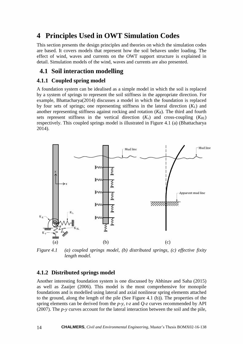
4.1.1 Coupled spring model
A foundation system can be idealised as a simple model in which the soil is replaced
by a system of springs to represent the soil stiffness in the appropriate direction. For
example, Bhattacharya(2014) discusses a model in which the foundation is replaced
by four sets of springs; one representing stiffness in the lateral direction (KL) and
another representing stiffness against rocking and rotation (KR). The third and fourth
sets represent stiffness in the vertical direction (Kv) and cross-coupling (KRL)
respectively. This coupled springs model is illustrated in Figure 4.1 (a) (Bhattacharya
2014).
(a) (b) (c)
Figure 4.1 (a) coupled springs model, (b) distributed springs, (c) effective fixity
length model.
4.1.2 Distributed springs model
Another interesting foundation system is one discussed by Abhinav and Saha (2015)
as well as Zaaijer (2006). This model is the most comprehensive for monopile
foundations and is modelled using lateral and axial nonlinear spring elements attached
to the ground, along the length of the pile (See Figure 4.1 (b)). The properties of the
spring elements can be derived from the p-y, t-z and Q-z curves recommended by API
(2007). The p-y curves account for the lateral interaction between the soil and the pile,
CHALMERS, Civil and Environmental Engineering, Master’s Thesis BOMX02-16-138 15
whereas the vertical interaction is accounted for using t-z curves which represent pile
skin friction. The Q-z curves account for end bearing.
4.1.3 Effective /Apparent fixity model
This model is discussed by Zaaijer (2006) and it is well suited for monopile
foundations. The soil-pile environment is represented by a clamped model of the pile
at an effective length below the seabed (see Figure 4.1 (c)). In this model, the pile is
not fixed at the original mud line but rather at a lower depth. This point is known as
the point of effective fixity for the cantilever pile. Kühn, cited in Zaaijer (2006)
suggests that the effective length should be between 3.3 and 3.7 times the pile
diameter.
To reduce the computational time and effort required to simulate the foundations,
these models need to be as simple as possible. However, a reasonable degree of
accuracy should also be maintained. Such requirements often complicate the process
of OWT foundation design. Bhattacharya (2014) notes that OWTs have to resist
moments that are disproportionately larger than the vertical loads and due to the
dynamic nature of the loads, the fatigue risk is considerably high.
4.2 Wind modelling and aerodynamic loads
Aerodynamic loads mainly result from wind turbulence and can either be direct or
indirect. Their magnitude depends on the turbulent wind speed. In this section,
definitions of wind fields and their interaction with the OWT structure (aerodynamic
loads) will be presented.
According to Matha et al. (2010), aerodynamic loads can be further grouped into three
categories;
- Steady aerodynamic loads due to mean wind speed
- Periodic aerodynamic loads due wind shear, rotor rotation, off-axis winds and
tower shadowing
- Randomly fluctuating aerodynamic loads resulting from gusts, turbulence and
dynamic effects.
Wind fields can be described in deterministic and stochastic approaches. The
deterministic approach is based on real data measured from a specific site and specific
conditions. It can be utilised to investigate the behaviour of the structure in extreme
conditions (Passon and Kühn 2005). On the other hand, the stochastic approach is
based on probabilistic methods to describe wind field. It is also the stochastic
approach that is the most appropriate for calculating fatigue loads.
4.2.1 Stochastic wind profiles
According to DNV (2010), in case the measured wind data is insufficient to establish
site-specific spectral densities, the wind speed process can be represented by the
following spectra.

CHALMERS, Civil and Environmental Engineering, Master’s Thesis BOMX02-16-138 16
- Davenport spectrum
This spectrum expresses spectral densities in terms of the 10 minute mean wind speed
irrespective of the elevation. The Davenport spectrum is represented by the following
spectral density function;
3/42
10
2
102
.1
3
2
)(
U
Lf
fU
L
fS
U
U
Uu (4.1)
where 𝑓 is the frequency and 𝐿𝑈 is the length scale of the wind speed. The DNV
(2010) also specifies that this spectrum is developed for wind over land with 𝐿𝑈 of
1200 m. 𝜎𝑈 is the standard deviation of the wind speed.
However, this spectrum is not appropriate for use in the low frequency range (less
than 0.01 Hz). What is noted too is that it is difficult to consider the Davenport
spectrum when analysing data in this range, due to the abrupt fall in the spectral
density value of the Davenport spectrum in the vicinity of zero frequency.
- Kaimal spectrum
The Kaimal spectrum has the following expression;
3/5
10
102
.32.101
868.6
U
Lf
U
L
fS
U
U
Uu (4.2)
Again here, 𝑓 denotes the frequency but 𝐿𝑈 is the integral length scale which can be
computed as;
0ln074.046.0
300300
z
U
zL
(4.3)
where 𝑧 is the height above the ground or the sea and 𝑧0 is the terrain roughness.
IEC (2005) proposes an alternative integral length independent of the terrain
roughness as;
𝐿𝑈 = 3.33 𝑧 𝑓𝑜𝑟 𝑧 < 60 𝑚200 𝑚 𝑓𝑜𝑟 𝑧 ≥ 60 𝑚
- The Harris spectrum
Similar to the Davenport spectrum, the Harris spectrum defines the spectral density
without considering the elevation as follows;
6/5
2
10
102
8.701
4
U
fL
U
L
fS
U
U
UU (4.4)

CHALMERS, Civil and Environmental Engineering, Master’s Thesis BOMX02-16-138 17
where 𝐿𝑈 is the integral length scale in the range 60-400 m with a mean value of
180m. If there is no data indicating otherwise, 𝐿𝑈 can be calculated as for the Kaimal
spectrum. The DNV reports that this spectrum is originally developed for turbines
over land and is not suitable in the low frequency range (𝑓 < 0.01 𝐻𝑧).
- Von Karman spectrum
The Von Karman spectrum is another alternative for defining wind profiles and is one
of the most commonly used methods in OWT simulation. DNV(2010) expresses the
Von Karman spectrum as follows;
65
2
2
))/(8.701(
/4)(
wv
wvU
Karman
VfL
VLfS
(4.5)
where σu stands for the standard deviation of the wind speed (m/s) and Vw is the mean
wind speed (m/s). Similar to the other spectra mentioned above, Lv represents integral
length scale (m) and f means frequency (Hz).
- Other spectra
In addition to the spectra discussed, the DNV (2010) says that the empirical Simiu and
Leigh spectrum as well as the empirical Ochi and Shin spectrum may be applied to the
design of offshore structures. The Simiu and Leigh spectrum takes into account the
wind energy over a seaway in the low frequency range. Similarly, the Ochi and Shin
spectrum is developed from measured spectra over a seaway and it has more energy
content in the low frequency range than the Kaimal, Harris and Davenport spectra.
4.2.2 Aerodynamic loads
There are some methods developed to calculate the wind load acting on OWTs by
describing a relation between the wind profile and the blades of the structure.
Simulation codes for OWTs generally utilise Blade Element Momentum (BEM)
theory or Generalised Dynamic Wake (GDW) theory.
- Blade element momentum theory
Blade element momentum theory is the most common aerodynamic load calculation
method in OWT design that calculates the velocity change imposed by wind flow. In
fact, it is a combination of blade element theory and momentum theory. Moriarty and
Hansen (2005) defined blade element theory as a method that divides the blade into
small independent elements and lets the blade act as a two-dimensional aileron and
then calculates the aerodynamic forces acting on each element from the local flow.
For momentum theory, Moriarty and Hansen also added that the momentum theory
assumes that the loss of pressure and momentum in the rotor plane is the result of the
work performed by the airflow which migrates through the blades (2005). The
velocity change of the blades in axial and tangential directions can be calculated
based on the work done by airflow. Therefore, one can assert that blade element
momentum theory is a method that utilises the blade element theory considering the
changes in the airflow. These changes are calculated using the momentum theory.
Like all theories used in OWT design, BEM has some limitations too. One limitation
is that since the momentum theory considers momentum equilibrium in the rotor
plane, BEM theory fails to give proper results if the blades deflect out of the rotor
CHALMERS, Civil and Environmental Engineering, Master’s Thesis BOMX02-16-138 18
plane (Moriarty and Hansen 2005). Another limitation is that BEM does not consider
wind flow definition along the span since it only assumes two-dimensional wind flow.
Another limitation is that BEM theory is only capable of linear analysis and therefore,
it does not consider time lag effects when the wind speed or direction changes. Apart
from that, BEM theory needs some modifications to define tip losses and wake
aerodynamics.
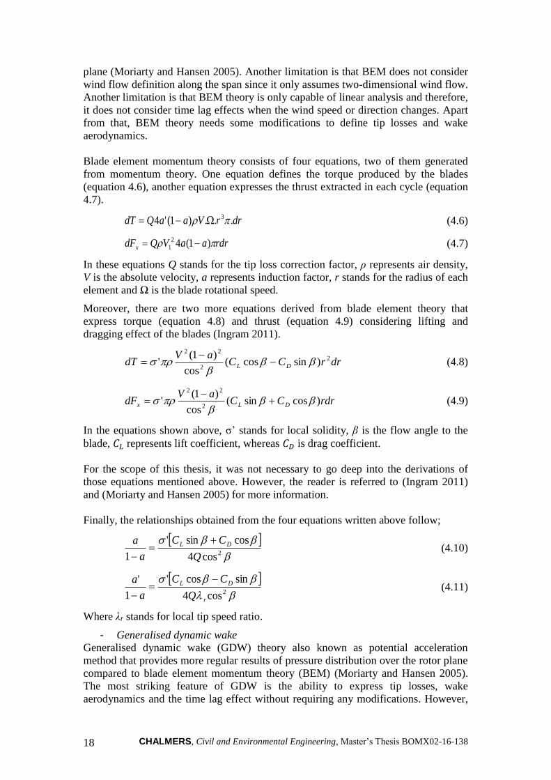
Blade element momentum theory consists of four equations, two of them generated
from momentum theory. One equation defines the torque produced by the blades
(equation 4.6), another equation expresses the thrust extracted in each cycle (equation
4.7).
drrVaaQdT ...)1('4 3 (4.6) (1)
rdraaVQdFx )1(42
1 (4.7)
In these equations Q stands for the tip loss correction factor, ρ represents air density,
V is the absolute velocity, a represents induction factor, r stands for the radius of each
element and Ω is the blade rotational speed.
Moreover, there are two more equations derived from blade element theory that
express torque (equation 4.8) and thrust (equation 4.9) considering lifting and
dragging effect of the blades (Ingram 2011).
drrCCaV
dT DL
2
2
22
)sincos(cos
)1('
(4.8)
rdrCCaV
dF DLx )cossin(cos
)1('
2
22
(4.9)
In the equations shown above, σ’ stands for local solidity, β is the flow angle to the
blade, 𝐶𝐿 represents lift coefficient, whereas 𝐶𝐷 is drag coefficient.
For the scope of this thesis, it was not necessary to go deep into the derivations of
those equations mentioned above. However, the reader is referred to (Ingram 2011)
and (Moriarty and Hansen 2005) for more information.
Finally, the relationships obtained from the four equations written above follow;
2cos4
cossin'
1 Q
CC
a
a DL
(4.10)
2cos4
sincos'
1
'
r
DL
Q
CC
a
a
(4.11)
Where λr stands for local tip speed ratio.
- Generalised dynamic wake
Generalised dynamic wake (GDW) theory also known as potential acceleration
method that provides more regular results of pressure distribution over the rotor plane
compared to blade element momentum theory (BEM) (Moriarty and Hansen 2005).
The most striking feature of GDW is the ability to express tip losses, wake
aerodynamics and the time lag effect without requiring any modifications. However,

CHALMERS, Civil and Environmental Engineering, Master’s Thesis BOMX02-16-138 19
this method also has some limitations. GDW theory is not appropriate for heavily
loaded rotors due to the assumption that if the propagated velocities are smaller than
the mean flow, an instability occurs when the turbulent wake state is reached at lower
wind speeds (Laino and Hansen, cited in Moriarty and Hansen 2005).
- Dynamic stall effect
Aerofoils under unsteady flow conditions with a periodically varying angle of attack
exhibit aerodynamic characteristics that are different from those under steady flow
conditions. This phenomenon is known as dynamic stall during which the aerofoil is
oriented at an angle greater than the critical angle of wind attack. The resulting effect
is characterised by airflow dispersion at the suction side of the aerofoil and causes an
increase in the drag on the aerofoil. According to Vahdati et al. (2011), this
phenomenon is more common in vertical axis wind turbines than in horizontal axis
wind turbines. The blades are consequently subjected to recurring forces due the
variation of incidence angle of the wind direction. Although the effect of dynamic
stall at low tip speed ratios is an advantage in terms of power generation, the
formation of vortexes causes extremely undesirable circumstances like vibrations,
noise and a reduction in fatigue life of the blades due to unsteady forces.
4.3 Wave modelling and hydrodynamic loads
Henderson et al. (2003) reckon that the calculation and determination of design wave
loads on an OWT structure is a complex process that involves different wave models,
load calculation methods and probability analyses. Still, it is important for a designer
to go through this process in order to produce a cost effective and durable structural
design. It is therefore important to understand the waves, their distribution and
hydrodynamic properties.
The procedure of wave load calculation can be intended for peak loads or fatigue
loads and is divided into three stages;
Describing the wave and wave climate
Selecting an appropriate wave load calculation procedure
Computing the load effect.
According to Le Mehaute (1976), the choice of wave model depends on the wave type
and the range of values of the parameters H/L, H/d and L/d where H, L and d are the
wave height, wave length and water depth respectively. Three mathematical
approaches are used to model wave characteristics, namely; linearization, power
series and numerical methods. These are known as deterministic models. In addition,
statistical (stochastic) methods can also be used to describe the complexity of sea
states and waves generated by wind.
4.3.1 Deterministic wave models
- Linear wave theory (Airy)
Linear wave theories are the simplest case of water wave theories in which the
convective inertia terms of the wave equation are completely ignored. A classic
example of linear wave theories is the Airy wave model according to Airy (1845).
Linear wave theories are only valid if the wave height is considerably small compared
to wavelength and still water depth. The linear wave theory is relatively simple but

CHALMERS, Civil and Environmental Engineering, Master’s Thesis BOMX02-16-138 20
lacks accuracy and its primary weakness is that it truncates the wave peaks and
troughs. However if integrated with other properties of the wave-load calculation for
example stochastic waves, diffraction and some correction, its accuracy can be
improved (Henderson et al. 2003).
- Wheeler stretching
This is generally a correction to the linear wave theory where the kinematics of the
wave as calculated at the mean-water level are applied to the true surface with the
distribution down to the seabed. This theory improves the prediction of wave
kinematics which can be also applied to stochastic models (Henderson et al. 2003). In
Chapter 5, the linear wave theory with such surface improvement (Wheeler
stretching) is denoted as Airy+.
- Power series (Stokes and Cnoidal waves)
For cases where waves are too steep or water depths are too shallow, it is not practical
to use the linear theory. Under such circumstances, the choice is to use higher order
approximations in which the waves are modelled as a power series in terms of a
characteristic parameter. This parameter is H/L in deep waters or H/d in shallow
water. The former case is a characteristic of Stokes theory (2nd, 3rd and 5th order) and
the first term of the power series is a solution of the linearised equations. The later
parameter describes the Cnoidal theory in which the first term of the series constitutes
the solution of nonlinear equations. These methods are not commonly used because of
the complexity of dealing with terms of the series. Detailed discussions of these wave
theories are given by Le Mehaute (1976) and (Fenton 1988).
- Numerical wave models (Dean’s stream function and Fenton’s model)
It is possible that no solution of the steady-state wave profile exists. For such a case, it
is only possible to employ a numerical solution where the differentials are replaced by
finite differences. According to Le Mehaute (1976), this is typical for very large
values of H/L and H/d and consequently when the nonlinear terms are rather large
compared to the local inertia. This happens commonly with long waves in very
shallow water.
One of the most common numerical wave models is Dean’s Stream Function,
developed by Dean (1965) for the purpose of numerically examining fully non-linear
water waves. The method computes a series of solutions to the fully nonlinear water
wave problem involving the Laplace equation with two non-linear free surface
boundary conditions (constant pressure and wave height).
Of course, a numerical approach such as the Stream Function can be used to solve
linearised equations. In fact, the stream function is considered more accurate than the
linear theory when it comes to simulating considerably large but linear waves.
Various studies have brought out other advantages of the stream function; it has been
shown that the stream function description of non-linear waves is the best when
relatively shallow waters are considered (Eecen 2003).
The Fenton model is very similar to the stream function wave theory developed by
Dean (1965). It is based on a system of rational approximations by Stokes theory and
Cnoidal theory (Fenton 1988). The former makes the assumption that all variation in
the horizontal direction can be represented by Fourier series, the coefficients being

CHALMERS, Civil and Environmental Engineering, Master’s Thesis BOMX02-16-138 21
expressed as perturbation expansions in terms of a parameter which increases with the
wave height i.e. H/L.
4.3.2 Stochastic wave models
In reality, the sea is never in a regular state that has a constant wave height and length.
Therefore, there is a need for more developed wave definitions to describe irregular
sea waves in OWT design. Irregular sea states however can be defined with a
combination of regular sea waves where the energy of the sea state must be the same
as the sum of the energies of all subsidiary waves.
The energy distribution of a sea state can be described by a frequency spectrum, it is
then also possible to observe the individual contribution of each subsidiary wave to
the total energy. According to Lucas and Guedes Soares (2015), the wind force on the
waves generates nonlinear interactions between waves which induce energy transfer
across energy bands leading to spectra that are similar for a given level of sea state
development. The most frequently used spectra to describe waves are; Pierson-
Moskowitz spectrum and JONSWAP spectrum. However, there are many more that
can be employed and these include; the Constrained NewWave spectrum,
Bretschneider spectrum etc.
- Pierson-Moskowitz distribution
This was developed by Pierson and Moskowitz and has gained general acceptance for
its adequacy to describe the spectra of fully developed sea states and therefore
representing the balance between the forcing of the wind and wave conditions (Lucas
and Guedes Soares 2015). According to Pierson and Moskowitz (1964), the wave
function is of the form;
4
0
5
2
exp.
gS (4.12)
f.2 ;
31
0 Ug
where 𝑓 is the wave frequency, 𝛼 and 𝛽 are constants, while 𝑈1/3 is the velocity of
wave at the significant wave height. Figure 4.2 illustrates the wave form at different
wind speeds.

CHALMERS, Civil and Environmental Engineering, Master’s Thesis BOMX02-16-138 22
Figure 4.2 Wave spectra of a fully developed sea for different wind speeds.
A fully developed sea is assumed in which the waves are in equilibrium with the
wind. This is based on an assumption that the wind blows steadily for a long time
over a large area.
- JONSWAP Spectrum
This distribution was developed in a joint research project called the Joint North Sea
Wave Project. During the project, Hasselmann et al. (1973) observed that a wave
spectrum is never fully developed but rather it continues to develop through non-
linear, wave-to-wave interactions even for longer periods and distances. This
observation resulted into a spectrum of the form;
rpgS
4
5
2
4
5exp
. (4.13)
22
2
2exp
p
pr
(4.14)
31
10
2
22
FUg
p (4.15)
In the expressions above, 𝐹 is the fetch (distance) over which the wind blows with
constant velocity and 𝜎 is defined as;
0
20
40
60
80
100
120
0.00 0.05 0.10 0.15 0.20 0.25 0.30
Wav
e sp
ectr
al D
ensi
ty (
m2/H
z)
Frequency (Hz)
20.6 m/s
18 m/s
15.4 m/s
12.9 m/s
10.3 m/s

CHALMERS, Civil and Environmental Engineering, Master’s Thesis BOMX02-16-138 23
𝜎 = 0.07 𝑓𝑜𝑟 𝜔 ≤ 𝜔𝑝
0.09 𝑓𝑜𝑟 𝜔 > 𝜔𝑝
Figure 4.3 shows a series of JONSWAP Spectra for different fetches.
Figure 4.3 Wave spectra of a developing sea for different fetches.
It can be seen that this spectrum is actually a form of the Pierson-Moskowitz
distribution enhanced by a peak factor, 𝛾. During the development of the sea states,
there is a higher concentration of energy around the dominant frequency and the
spectrum appears more peaked than the Pierson-Moskowitz spectrum. This high
concentration of energy is effected by a peak enhancement factor included in the
expression.
- New Wave model
The New Wave theory as discussed by Tromans et al. (1991) involves modelling the
sea surface using Gaussian statistics. It accounts for the spectral composition of the
sea and can be used as an alternative to both regular waves and full random time
domain simulations of lengthy time histories. Tromans et al. (1991) conclude that the
theory provides a rational model for the extreme waves of a sea state.
According to Cassidy et al. (2001), the surface elevation around an extreme wave
event (for instance a crest) can be modelled by the statistically most probable shape
associated with its occurrence. Tromans et al. (1991) show that the surface elevation
follows a normal distribution about the most probable shape. The surface elevation is
represented by two terms, one deterministic and another random as follows;
gr .)( (4.16)
0
0.1
0.2
0.3
0.4
0.5
0.6
0 0.1 0.2 0.3 0.4 0.5 0.6 0.7
Wav
e sp
ectr
al D
ensi
ty (
m2/H
z)
Frequency (Hz)
γ=11
γ=10
γ=9
γ=7
γ=5
CHALMERS, Civil and Environmental Engineering, Master’s Thesis BOMX02-16-138 24
In the expression, the first term represents the most probable value. 𝛼 is the crest
elevation and 𝑟(𝜏) is the autocorrelation function for the ocean surface elevation
which is proportional to the inverse Fourier Transform of the surface energy
spectrum. 𝜏 is the relative time of the extreme event to the initial starting time. The
second term in the expression is a non-stationary Gaussian process with a mean of
zero and standard deviation that increases from zero at the crest to 𝜎 (the standard
deviation of the underlying sea at a distance away from the crest). Cassidy et al.
(2001) observe that as the crest elevation increases, the first term becomes dominant
and can be used on its own in deriving the surface elevation and wave kinematics near
the crest.
According to Cassidy et al. (2001), the autocorrelation function is defined as
0
ieSr (4.17)
From the discussion, it is evident that this wave model has both deterministic and
stochastic properties.
4.3.3 Hydrodynamic loads
Hydrodynamic loads on an OWT can be computed using a number of methods
including Morison equation, potential flow theory, diffraction theory and computation
fluid dynamics.
4.3.3.1 Morison equation
Morrison’s equation is effective for wave loads on slender structures like monopiles
and braced structures and it is defined as;
21
2 4t D M D M
Df f f C Du u C u
(4.18)
Where 𝑓𝑡is the force acting on the structure and 𝑓𝐷 and 𝑓𝑀 are drag and inertia forces
respectively, 𝐶𝐷 is the drag coefficient, 𝐶𝑀 is the inertia coefficient and 𝑢 is the
horizontal water particle velocity while is the horizontal water particle acceleration.
𝜌 is the density of water and 𝐷 is the diameter of the structure in the water.
The validity of Morison equation is based on the assumption that the structure is small
compared to the wave length of the water. Therefore, for massive structures in
relatively shallow water, the accuracy of Morrison’s equation is compromised since in
such cases the structure has an influence on the wave field. It is then more appropriate
to use the potential flow theory or modify the Morrison equation (MacCamy-Fuch,
cited in Passon and Kühn 2005). In addition, the Morrison equation is limited by its
inability to consider surface effects and the three dimensional effects of loads on the
structure.
4.3.3.2 Potential flow theory
Potential flow is also known as irrotational flow in which the fluid is considered
inviscid (negligible viscous effects). Viscous effects are considered negligible for

CHALMERS, Civil and Environmental Engineering, Master’s Thesis BOMX02-16-138 25
flows at a high Reynold’s number dominated by convective momentum transfer.
Therefore, potential flow is useful for analysing external flows over solid surfaces at
considerably high Reynold’s number (rapid flow), given that the flows still remain
laminar. The principle assumption is when the flow is over a surface is rapid, the
viscous boundary layer region that forms next to the surface is very thin and therefore
this boundary layer can be neglected. This implies that the potential flow can be
assumed to follow the contours of the solid surface, as if the boundary layer was not
present.
Potential flow theory is characterised by two concepts; the velocity potential function
( V ) and the Stream function ( V ). For more details about the mathematics
of potential flow, the reader is referred to (White 2003).
4.3.3.3 Diffraction theory
The diffraction theory can also be used to study the wave forces on a body situated in
water. The theory assumes that if the typical dimension of a body is considerably
larger in relation to the wavelength and the wave height, then the effects of dispersion
due to viscosity can be regarded as negligible and diffraction effects are assumed to
be dominant. Another assumption is that the water flow is incompressible and non-
rotational, and that the surface tension effects are negligible. A combination of these
assumptions means that the flow can be described by a scalar velocity potential which
in turn satisfies Laplace’s equation within the fluid domain (Le Mehaute 1976).
4.3.3.4 Computational fluid dynamics
Computational fluid dynamics (CFD) is a branch of physics that deals with numerical
modelling and simulation of fluid flow. It thus provides a qualitative prediction of
fluid flow through numerical methods and mathematical models which can be
implemented into computer solvers to further save time.
4.4 Currents
According to DNV GL (2014a), current velocities can be treated with three different
current models including; near surface currents, sub surface currents and near shore
currents.
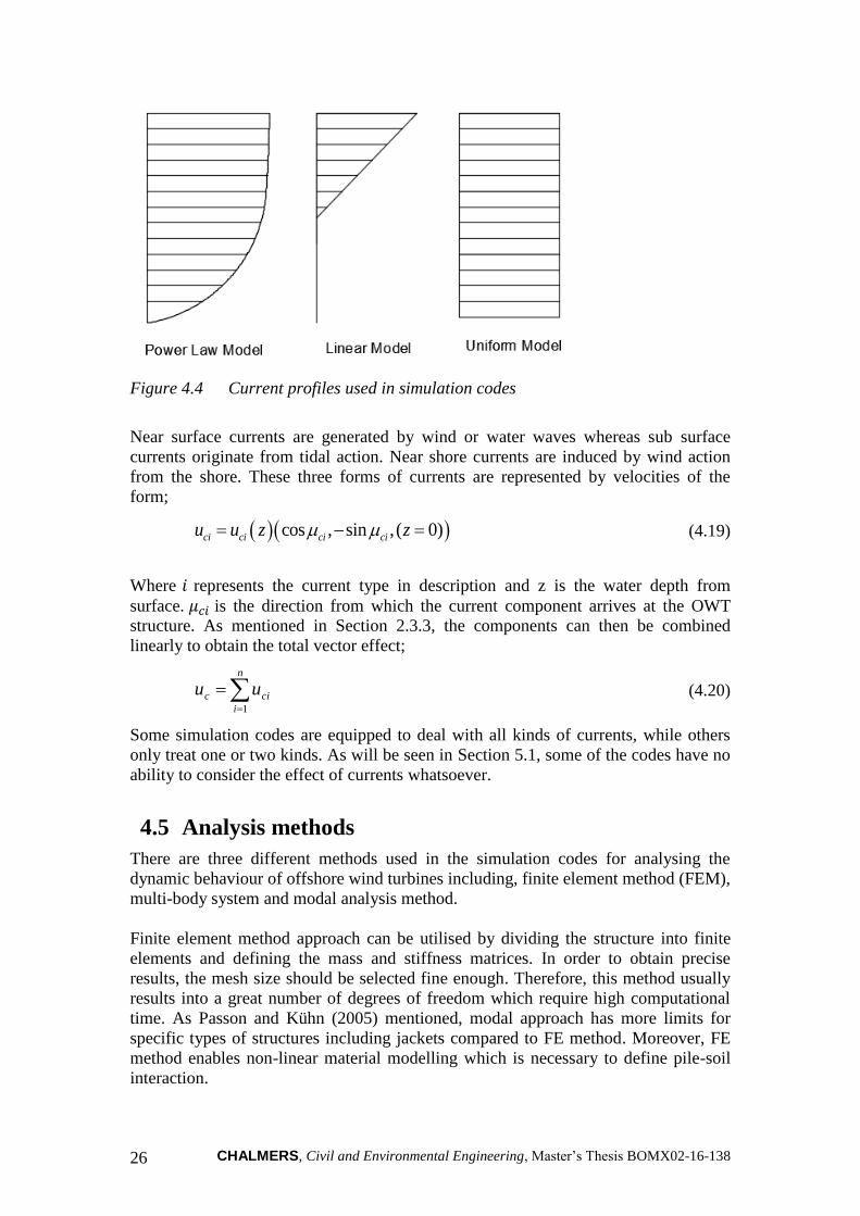
Near surface currents adopt a current profile following a power law that changes the
shape of the current profile exponentially with depth. Moreover, sub surface currents
employ a linear relationship down to a certain depth and remains stable. Near shore
currents, however, assume a fixed current profile independently from the depth.
CHALMERS, Civil and Environmental Engineering, Master’s Thesis BOMX02-16-138 26
Figure 4.4 Current profiles used in simulation codes
Near surface currents are generated by wind or water waves whereas sub surface
currents originate from tidal action. Near shore currents are induced by wind action
from the shore. These three forms of currents are represented by velocities of the
form;
cos , sin ,( 0)ci ci ci ciu u z z (4.19)
Where 𝑖 represents the current type in description and z is the water depth from
surface. 𝜇𝑐𝑖 is the direction from which the current component arrives at the OWT
structure. As mentioned in Section 2.3.3, the components can then be combined
linearly to obtain the total vector effect;
n
i
cic uu1
(4.20)
Some simulation codes are equipped to deal with all kinds of currents, while others
only treat one or two kinds. As will be seen in Section 5.1, some of the codes have no
ability to consider the effect of currents whatsoever.
4.5 Analysis methods
There are three different methods used in the simulation codes for analysing the
dynamic behaviour of offshore wind turbines including, finite element method (FEM),
multi-body system and modal analysis method.
Finite element method approach can be utilised by dividing the structure into finite
elements and defining the mass and stiffness matrices. In order to obtain precise
results, the mesh size should be selected fine enough. Therefore, this method usually
results into a great number of degrees of freedom which require high computational
time. As Passon and Kühn (2005) mentioned, modal approach has more limits for
specific types of structures including jackets compared to FE method. Moreover, FE
method enables non-linear material modelling which is necessary to define pile-soil
interaction.

CHALMERS, Civil and Environmental Engineering, Master’s Thesis BOMX02-16-138 27
The modal analysis method in OWT design is the fastest option compared to the other
methods. The structure is defined with a low number of eigenmodes by deselecting
some degrees of freedom. Although the modal analysis method is computationally
efficient due to having a low number of degrees of freedom, it has some limitations
such as having the same type of degrees of freedom and only being capable of linear
analysis (Passon and Kühn 2005).
As for the multi-body system, the structure is separated into finite elements in a way
similar to the FE method. Apart from that, those elements usually consist of rigid
bodies that are connected together with elastic joints. According to Passon and Kühn,
the multi-body system associates the advantages of the modal approach and FE
method by being capable of non-linear analysis while keeping the set of equations
considerably small (2005).
The calculations for OWT structures can be done in both time domain and frequency
domain in the context of different benefits. Time domain is the more frequently
adopted calculation method in the industry in which the response of the structure
(stress, strain, moment, deflection, etc.) is extracted for a certain time interval.
However, since offshore environmental conditions (wind speed, wind direction, wave
frequency and length, etc.) vary significantly over time, fatigue analysis for OWTs
generates very time-consuming calculations. Therefore, calculations in the frequency
domain become more efficient (van Engelen & Braam 2004). Moreover, frequency
domain analysis is a good preliminary study to understand the response of the
structure in a certain environment and define the frequency interval which the OWT
structure must stay in. In order to perform a frequency domain analysis, sufficient
data is needed to describe the behaviour of the environmental effects.
4.6 Analysis techniques
Analysis approaches also play an important role in OWT design. The most common
design approaches can be classified into three categories such as; sequential approach,
semi-coupled loads approach and fully coupled loading approach.
4.6.1 Sequential approach technique
In the sequential approach, the OWT structure is separated into its subsystems such as
blades, rotor, tower and support structure. The core idea behind this approach is that
each subsystem of the OWT requires different assumptions and approaches, therefore,
it is more time efficient to treat them in isolated models. Such an approach introduces the necessity to exchange information regarding
structural properties of all relevant subsystems as well as loads at one or more
predefined interfaces, often the connection between the tower and foundation
subsystem. (Passon and Branner 2013, p.435) Moreover, Zarafshan and Hall (2015) explain the application process as following;
- First, wave loads are applied to the substructure and foundation and then the
internal forces at the interface are transferred to aero-elastic models.
- Secondly, wind loads are applied to the aero-elastic model and resultant force
at the tower-substructure interface is recorded.
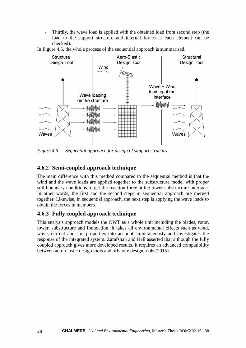
CHALMERS, Civil and Environmental Engineering, Master’s Thesis BOMX02-16-138 28
- Thirdly, the wave load is applied with the obtained load from second step (the
load to the support structure and internal forces at each element can be
checked).
In Figure 4.5, the whole process of the sequential approach is summarised.
Figure 4.5 Sequential approach for design of support structure
4.6.2 Semi-coupled approach technique
The main difference with this method compared to the sequential method is that the
wind and the wave loads are applied together to the substructure model with proper
soil boundary conditions to get the reaction force at the tower-substructure interface.
In other words, the first and the second steps in sequential approach are merged
together. Likewise, in sequential approach, the next step is applying the wave loads to
obtain the forces in members.
4.6.3 Fully coupled approach technique
This analysis approach models the OWT as a whole unit including the blades, rotor,
tower, substructure and foundation. It takes all environmental effects such as wind,
wave, current and soil properties into account simultaneously and investigates the
response of the integrated system. Zarafshan and Hall asserted that although the fully
coupled approach gives more developed results, it requires an advanced compatibility
between aero-elastic design tools and offshore design tools (2015).

CHALMERS, Civil and Environmental Engineering, Master’s Thesis BOMX02-16-138 29
Figure 4.6 Integrated system with environmental effects

CHALMERS, Civil and Environmental Engineering, Master’s Thesis BOMX02-16-138 30
5 Simulation Codes and Classification
In this chapter the reader is introduced to some of the current simulation codes used in
OWT design in connection with Chapter 4 that presents the principles used in each
code, respectively. Moreover, the classification of codes that expresses the design
principles and methodologies is shown.
5.1 Current simulation codes in use
5.1.1 FAST (Fatigue, Aerodynamics, Structures and Turbulence)
Fast was created by the National Renewable Energy Laboratory (NREL) of USA and
has evolved over two decades to increase its capabilities. The latest version FAST v8
incorporates several modules, such as: AeroDyn (ADAMS/WT) for aerodynamics;
ServoDyn for electrical drive dynamics; SubDyn for structural dynamics; HydroDyn
for hydrodynamics; MAP for mooring dynamics and IceFloe for ice loads, which is a
big change in the architecture of the software compared to FAST v7. Main features of
FAST are shown below:
- Prediction of fatigue loads for both two and three bladed systems.
- Aeroacoustic noise predictions.
- Ability of defining lateral offset, rotor furling and yaw control.
- Dynamic stationary simulations
The general specifications of the code are shown in Table 5.1.

CHALMERS, Civil and Environmental Engineering, Master’s Thesis BOMX02-16-138 31
Table 5.1 The main specifications of FAST.
Specification Adopted Principle Reference
En
vir
on
men
tal
Act
ion
s Deterministic Wave
Airy and possible
modifications for surface
effects (Airy+)
Jonkman et al.
(n.d.)
Stochastic Wave Pierson-Moskowits,
JONSWAP, user defined
Sea Current Possible to define
Hydrodynamic
Loads
Morison equation (Strip-
Theory), Potential Flow
Theory
Aerodynamic Loads
Blade Element Momentum
Theory, Generalised Dynamic
Wake and Dynamic Stall
J.M. Jonkman,
G.J. Hayman,
B.J. Jonkman
(n.d.)
Str
uct
ura
l M
od
elli
ng
Analysis Method
Modal analysis and combined
modal-multi body dynamic
analysis
Passon and
Kühn (2005)
Analysis
Technique Fully coupled approach
Jonkman and
Jonkman
(2015) Time/Frequency
Domain
Calculations.
Time domain
Foundation Models Apparent fixity length
Passon and
Kühn (2005)
Su
pp
ort
Str
uct
ure
Typ
es
Tower Mono-tower, space frame
Foundation Monopile, space frame, gravity
based and floating
Foundation Support Monopile, general piles suction
caisson
Programming
Language
Intel® Visual Fortran
Composer Jonkman and
Jonkman
(2015) License and OS Open source / MS Windows,
Linux
5.1.2 Flex5
Flex5 is an open-source, extensively used offshore wind turbine simulation code
programmed in Turbo Pascal in early 1990s. The code mainly has the design
capabilities for monopile, mono-tower OWT structures. In terms of environmental
effects, similar to most of the other OWT simulation codes waves can be defined
either as deterministic or stochastic waves. Since there is a lack of user’s manual and
the software requires a license key, specifications of Flex5 could not be collected.
Therefore, previous studies were used to comprise the features of Flex5 in Table 5.2.
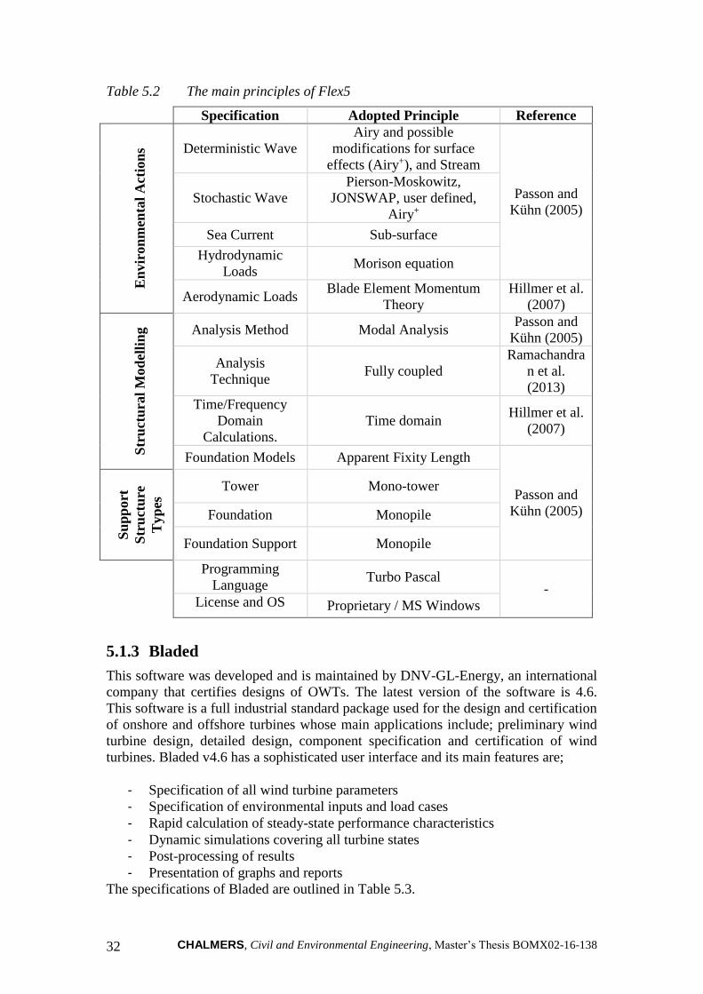
CHALMERS, Civil and Environmental Engineering, Master’s Thesis BOMX02-16-138 32
Table 5.2 The main principles of Flex5
Specification Adopted Principle Reference
En
vir
on
men
tal
Act
ion
s Deterministic Wave
Airy and possible
modifications for surface
effects (Airy+), and Stream
Passon and
Kühn (2005) Stochastic Wave
Pierson-Moskowitz,
JONSWAP, user defined,
Airy+
Sea Current Sub-surface
Hydrodynamic
Loads Morison equation
Aerodynamic Loads Blade Element Momentum
Theory
Hillmer et al.
(2007)
Str
uct
ura
l M
od
elli
ng
Analysis Method Modal Analysis Passon and
Kühn (2005)
Analysis
Technique Fully coupled
Ramachandra
n et al.
(2013)
Time/Frequency
Domain
Calculations.
Time domain Hillmer et al.
(2007)
Foundation Models Apparent Fixity Length
Passon and
Kühn (2005)
Su
pp
ort
Str
uct
ure
Typ
es Tower Mono-tower
Foundation Monopile
Foundation Support Monopile
Programming
Language Turbo Pascal
- License and OS Proprietary / MS Windows
5.1.3 Bladed
This software was developed and is maintained by DNV-GL-Energy, an international
company that certifies designs of OWTs. The latest version of the software is 4.6.
This software is a full industrial standard package used for the design and certification
of onshore and offshore turbines whose main applications include; preliminary wind
turbine design, detailed design, component specification and certification of wind
turbines. Bladed v4.6 has a sophisticated user interface and its main features are;
- Specification of all wind turbine parameters
- Specification of environmental inputs and load cases
- Rapid calculation of steady-state performance characteristics
- Dynamic simulations covering all turbine states
- Post-processing of results
- Presentation of graphs and reports
The specifications of Bladed are outlined in Table 5.3.

CHALMERS, Civil and Environmental Engineering, Master’s Thesis BOMX02-16-138 33
Table 5.3 The main principles of Bladed
Specification Adopted Principle Reference
En
vir
on
men
tal
Act
ion
s Deterministic Wave Airy+, Stream function.
DNV GL
(2014a),
DNV GL
(2014b),
Passon and
Kühn (2005)
Stochastic Wave
Pierson-
Moskowitz/JONSWAP and
Airy+, user defined,
Constrained New Wave
Sea Current
Subsurface, near surface, near
shore each separately or in
combination.
Hydrodynamic
Loads Morison Equation.
Aerodynamic Loads
Blade element momentum
theory and generalised
dynamic wake theory including
dynamic stall effects.
DNV GL
(2014a),
DNV GL
(2014b),
Str
uct
ura
l M
od
elli
ng
Analysis Method
Modal analysis combined with
modal–multi body dynamic
analysis.
DNV GL
(2014a)
Analysis
Technique Fully coupled
DNV GL
(2014a)
Time/Frequency
Domain
Calculations.
Time and frequency domain DNV GL
(2014a)
Foundation Models
Apparent fixity length and
distributed springs model
(treated as equivalent point
springs). DNV GL
(2014b),
Passon and
Kühn (2005)
Su
pp
ort
Str
uct
ure
Typ
es
Tower Mono-tower, arbitrary
space frame structure,
Foundation
Monopile, gravity base,
floating structures (with
mooring lines),
Foundation Support Monopile, suction caisson,
general pile
Programming
Language
VB6 with WPF interface,
Fortran and C++ code engine DNV GL
(2014b) License and OS Commercial / MS Windows 7
or higher
5.1.4 ADCoS
ADCoS stands for Aeroelastic and Dynamic Computation of Structures. This code
was developed by AeroDynamik Consult GmbH, an engineering consultancy service
provider related to wind energy. It has been in development since 1996 and its main
features include;
- Fatigue calculations

CHALMERS, Civil and Environmental Engineering, Master’s Thesis BOMX02-16-138 34
- Simulation of non-linear foundations. Nonlinear soil behaviour can be
calculated from commercial software like ALLPILE, L-PILE and added to
ADCoS as a non-linear pile element.
- Being able to define “Super-Element” in the model to describe any type of
structure by defining its mass and stiffness matrices.
The software uses ANSYS to define structural parameters and geometry; and use
ASAS module to calculate the loads from sea states. This software computes the
dynamic equation of motion using the finite element method. Each element is treated
as a 2 node-beam with each node having 6 degrees of freedom. In Table 5.4 the main
specifications of ADCoS are listed.
Table 5.4 The main principles of ADCoS
Specification Adopted Principle Reference
En
vir
on
men
tal
Act
ion
s Deterministic Wave
Airy and possible
modifications for surface
effects (Airy+) and Stream
Robertson et
al. (2014)
Stochastic Wave Pierson-Moskowitz user
defined, JONSWAP and Airy+
Passon and
Kühn (2005)
Sea Current Possible to define Vorpahl et al.
(2007)
Hydrodynamic
Loads Morison equation
Robertson et
al. (2014)
Aerodynamic Loads
Blade element momentum
theory, generalised dynamic
wake and dynamic stall
Jonkman and
Musial (2010)
Str
uct
ura
l M
od
elli
ng
Analysis Method Finite element method
Vorpahl et al.
(2007)
Analysis
Technique Sequential approach
Time/Frequency
Domain
Calculations.
Time domain
Foundation Models
Apparent fixity length and
discrete springs and user
defined
Su
pp
ort
Str
uct
ure
Typ
es
Tower Mono-tower and space frame
Passon and
Kühn (2005) Foundation
Monopile, space frame and
gravity base
Foundation Support Monopile, general pile
Programming
Language FORTRAN90
License and OS Commercial / MS Windows,
Linux
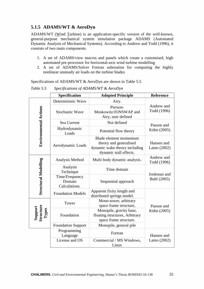
CHALMERS, Civil and Environmental Engineering, Master’s Thesis BOMX02-16-138 35
5.1.5 ADAMS/WT & AeroDyn
ADAMS/WT (Wind Turbine) is an application-specific version of the well-known,
general-purpose mechanical system simulation package ADAMS (Automated
Dynamic Analysis of Mechanical Systems). According to Andrew and Todd (1996), it
consists of two main components.
1. A set of ADAMS/view macros and panels which create a customised, high
automated pre-processor for horizontal-axis wind turbine modelling
2. A set of ADAMS/Solver Fortran subroutine for computing the highly
nonlinear unsteady air loads on the turbine blades
Specifications of ADAMS/WT & AeroDyn are shown in Table 5.5
Table 5.5 Specifications of ADAMS/WT & AeroDyn
Specification Adopted Principle Reference
En
vir
on
men
tal
Act
ion
s
Deterministic Wave Airy.
Andrew and
Todd (1996) Stochastic Wave
Pierson-
Moskowitz/JONSWAP and
Airy, user defined
Sea Current Not defined Passon and
Kühn (2005) Hydrodynamic
Loads Potential flow theory
Aerodynamic Loads
Blade element momentum
theory and generalised
dynamic wake theory including
dynamic stall effects.
Hansen and
Laino (2002)
Str
uct
ura
l M
od
elli
ng
Analysis Method Multi body dynamic analysis. Andrew and
Todd (1996)
Analysis
Technique Time domain
Jonkman and
Buhl (2005) Time/Frequency
Domain
Calculations.
Sequential approach
Foundation Models Apparent fixity length and
distributed springs model.
Passon and
Kühn (2005)
Su
pp
ort
Str
uct
ure
Typ
es
Tower Mono-tower, arbitrary
space frame structure,
Foundation
Monopile, gravity base,
floating structures, Arbitrary
space frame structure.
Foundation Support Monopile, general pile
Programming
Language Fortran
Hansen and
Laino (2002) License and OS Commercial / MS Windows,
Linux

CHALMERS, Civil and Environmental Engineering, Master’s Thesis BOMX02-16-138 36
NREL no longer supports ADAMS/WT and does not produce any more updates of it.
Instead, the functionality of ADAMS/WT has been replaced with an MSC.ADAMS
pre-processor that is now built into the FAST code (see Section 5.1.11). The FAST-
to-ADAMS pre-processor has all the functionalities of ADAMS/WT plus much more.
It works with the updated ADAMS-to-AeroDyn (A2AD) interface routines that are
part of the FAST modules.
5.1.6 HAWC2
HAWC2 (Horizontal Axis Wind turbine simulation Code 2nd generation) is an
aeroelastic code intended for analysing offshore wind turbine structures in time
domain. According to Larsen and Hansen (2007), the core of the code was developed
mainly within the years 2003-2006, by the Aeroelastic Design Research Program at
DTU Wind Energy, DTU Risø Campus in Denmark. HAWC2 is developed and
distributed by DTU Wind Energy and has been used in numerous research projects
and industrial applications. HAWC2 has a large number of users and is used for
design and verification purposes. Larsen and Hansen (2007) also asserted that the
code is based on a multibody formulation where each body is an assembly of
Timoshenko beam elements. The principles of HAWC2 can be seen in Table 5.6.

CHALMERS, Civil and Environmental Engineering, Master’s Thesis BOMX02-16-138 37
Table 5.6 The main principles of HAWC2
Specification Adopted Principle Reference
En
vir
on
men
tal
Act
ion
s Deterministic Wave Airy+, Stream Function.
Larsen and
Hansen (2007)
Stochastic Wave
Pierson-
Moskowitz/JONSWAP and
Airy+
Sea Current Constant, power law
Hydrodynamic
Loads Morison equation
Aerodynamic Loads
Blade element momentum
theory and generalised
dynamic wake theory including
dynamic stall effects.
Str
uct
ura
l M
od
elli
ng
Analysis Method Multi body dynamic analysis Passon and
Kühn (2005)
Analysis
Technique Fully coupled approach
Skaare et al.
(2006)
Time/Frequency
Domain
Calculations.
Time domain. Larsen and
Hansen (2007)
Foundation Models
Apparent fixity length,
Distributed springs model,
User defined.
Passon and
Kühn (2005)
Su
pp
ort
Str
uct
ure
Typ
es
Tower Mono-tower, arbitrary
space frame structure,
Foundation
Monopile, gravity base,
floating structures, arbitrary
space frame structure.
Foundation Support Monopile, general pile, user
defined.
Programming
Language Fortran
Larsen and
Hansen (2007) License and OS Commercial / MS-Windows,
Linux, Mac
5.1.7 ASHES
Ashes is a calculation tool for OWT design developed by Sismis AS (Norway). Ashes
is able to do time domain analysis which comes with a very user friendly interface to
show features of the model, such as loadings, deformations of the elements and blade
geometry etc. (Thomassen et al. 2012). The software is still under development, there
is no soil interaction definitions yet, but it is planned to include geotechnical
properties in the future versions of the software. The main specifications of Ashes are
outlined in Table 5.7.
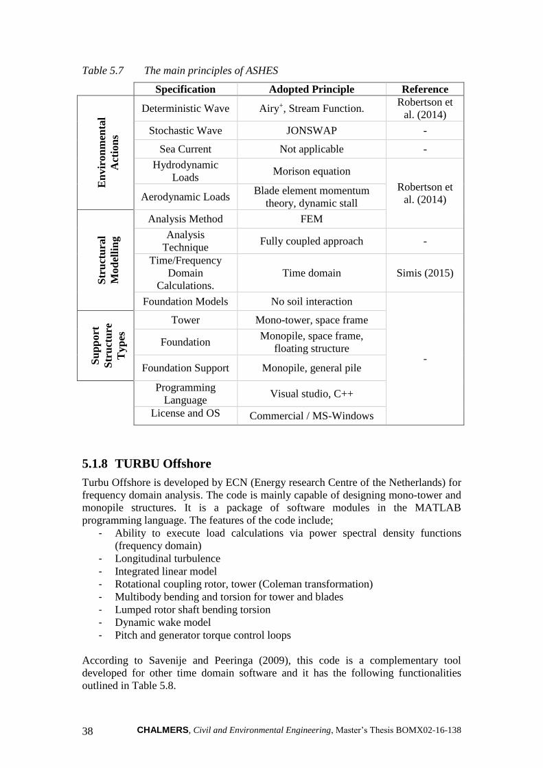
CHALMERS, Civil and Environmental Engineering, Master’s Thesis BOMX02-16-138 38
Table 5.7 The main principles of ASHES
Specification Adopted Principle Reference E
nvir
on
men
tal
Act
ion
s Deterministic Wave Airy+, Stream Function.
Robertson et
al. (2014)
Stochastic Wave JONSWAP -
Sea Current Not applicable -
Hydrodynamic
Loads Morison equation
Robertson et
al. (2014) Aerodynamic Loads Blade element momentum
theory, dynamic stall
Str
uct
ura
l
Mod
elli
ng
Analysis Method FEM
Analysis
Technique Fully coupled approach -
Time/Frequency
Domain
Calculations.
Time domain Simis (2015)
Foundation Models No soil interaction
- Su
pp
ort
Str
uct
ure
Typ
es
Tower Mono-tower, space frame
Foundation Monopile, space frame,
floating structure
Foundation Support Monopile, general pile
Programming
Language Visual studio, C++
License and OS Commercial / MS-Windows
5.1.8 TURBU Offshore
Turbu Offshore is developed by ECN (Energy research Centre of the Netherlands) for
frequency domain analysis. The code is mainly capable of designing mono-tower and
monopile structures. It is a package of software modules in the MATLAB
programming language. The features of the code include;
- Ability to execute load calculations via power spectral density functions
(frequency domain)
- Longitudinal turbulence
- Integrated linear model
- Rotational coupling rotor, tower (Coleman transformation)
- Multibody bending and torsion for tower and blades
- Lumped rotor shaft bending torsion
- Dynamic wake model
- Pitch and generator torque control loops
According to Savenije and Peeringa (2009), this code is a complementary tool
developed for other time domain software and it has the following functionalities
outlined in Table 5.8.

CHALMERS, Civil and Environmental Engineering, Master’s Thesis BOMX02-16-138 39
Table 5.8 Specifications of TURBU Offshore
Specification Adopted Principle Reference
En
vir
on
men
tal
Act
ion
s Deterministic Waves Airy
Savenije and
Peeringa
(2009)
Stochastic Waves
Pierson-
Moskowitz/JONSWAP and
Airy, User defined
Sea Current Accounted for
Hydrodynamic
Loads Morison equation
Aerodynamic Loads Blade element momentum
theory.
Str
uct
ura
l
Mod
elli
ng
Analysis Method Multi body dynamics
Analysis
Technique Fully coupled approach
Time/Frequency
Domain
Calculations.
Frequency domain
Foundation Models Apparent fixity length,
Distributed springs model
Su
pp
ort
Str
uct
ure
Typ
es Tower Mono-tower
Foundation Monopile
Foundation Support Monopile
Programming
Language MATLAB van Engelen
and Braam
(2004) License and OS Proprietary / Windows
5.1.9 FOCUS6
FOCUS6 is an integrated modular tool for designing wind turbines and wind turbine
components developed by WMC and includes software modules of ECN. It has been
in use for nearly two decades now and it is being used by wind turbine OEMs,
engineering companies for blade design, certification bodies, research institutes and
universities. FOCUS6 integrates onshore and offshore wind turbine design with blade
and support structure design (Knowledge Centre WMC 2016).
FOCUS6 has the following features;
- Interactive3D blade modeller
- Ultimate and fatigue strength analysis
- Modal analysis
- Finite element export (to ANSYS, MSC Marc, MSC Nastran, Abaqus)
- Finite element solver
- GL/GH Bladed4 interface
- Integrated design approach in which the wind turbine and support structure are
modelled and analysed as a whole.
- Offshore load generator

CHALMERS, Civil and Environmental Engineering, Master’s Thesis BOMX02-16-138 40
- Graphical post processing
- Aero elastic and hydro elastic structural design.
- 3D visualisation of results.
In operation, FOCUS6 integrates a number of module programs to analyse a given
wind turbine structure. For instance, it uses the PHATAS program (Lindenburg 2005)
to compute mechanical loads on wind turbines. Input for PHATAS comprises of
environmental conditions such as wind, waves, currents, etc. To generate random
linear waves to be used as input for the PHATAS program, Focus6 uses a program
called CurrentROWS (Random Ocean Wave Simulation) developed by ECN
(Peeringa 2013). In a similar fashion, the program Streamfunction is used to calculate
the wave kinematics of deterministic nonlinear waves (Eecen 2003).
The program SWIFT (Simulation of Wind Fields in Time) is used to numerically
simulate stochastic wind fields in the time domain whose resulting wind speed time
series can be used as input for any horizontal axis wind turbine design tool
(D.Winkelaar 1992). Similarly, the program Blademode is used to carryout aero
elastic analysis of the turbine (Lindenburg & Holierhoek 2013).
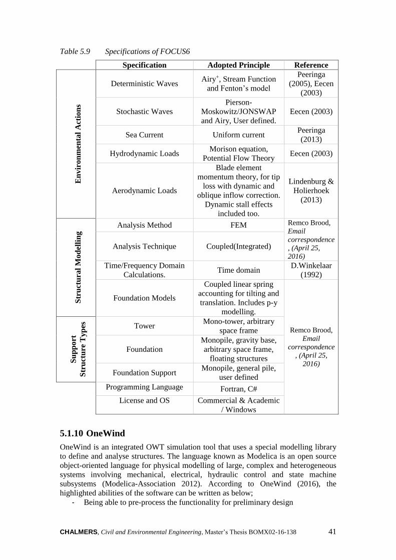
CHALMERS, Civil and Environmental Engineering, Master’s Thesis BOMX02-16-138 41
Table 5.9 Specifications of FOCUS6
Specification Adopted Principle Reference
En
vir
on
men
tal
Act
ion
s Deterministic Waves
Airy+, Stream Function
and Fenton’s model
Peeringa
(2005), Eecen
(2003)
Stochastic Waves
Pierson-
Moskowitz/JONSWAP
and Airy, User defined.
Eecen (2003)
Sea Current Uniform current Peeringa
(2013)
Hydrodynamic Loads Morison equation,
Potential Flow Theory Eecen (2003)
Aerodynamic Loads
Blade element
momentum theory, for tip
loss with dynamic and
oblique inflow correction.
Dynamic stall effects
included too.
Lindenburg &
Holierhoek
(2013)
Str
uct
ura
l M
od
elli
ng
Analysis Method FEM Remco Brood,
correspondence
, (April 25,
2016)
Analysis Technique Coupled(Integrated)
Time/Frequency Domain
Calculations. Time domain
D.Winkelaar
(1992)
Foundation Models
Coupled linear spring
accounting for tilting and
translation. Includes p-y
modelling.
Remco Brood,
correspondence
, (April 25,
2016) Su
pp
ort
Str
uct
ure
Typ
es
Tower Mono-tower, arbitrary
space frame
Foundation
Monopile, gravity base,
arbitrary space frame,
floating structures
Foundation Support Monopile, general pile,
user defined
Programming Language Fortran, C#
License and OS Commercial & Academic
/ Windows
5.1.10 OneWind
OneWind is an integrated OWT simulation tool that uses a special modelling library
to define and analyse structures. The language known as Modelica is an open source
object-oriented language for physical modelling of large, complex and heterogeneous
systems involving mechanical, electrical, hydraulic control and state machine
subsystems (Modelica-Association 2012). According to OneWind (2016), the
highlighted abilities of the software can be written as below;
- Being able to pre-process the functionality for preliminary design
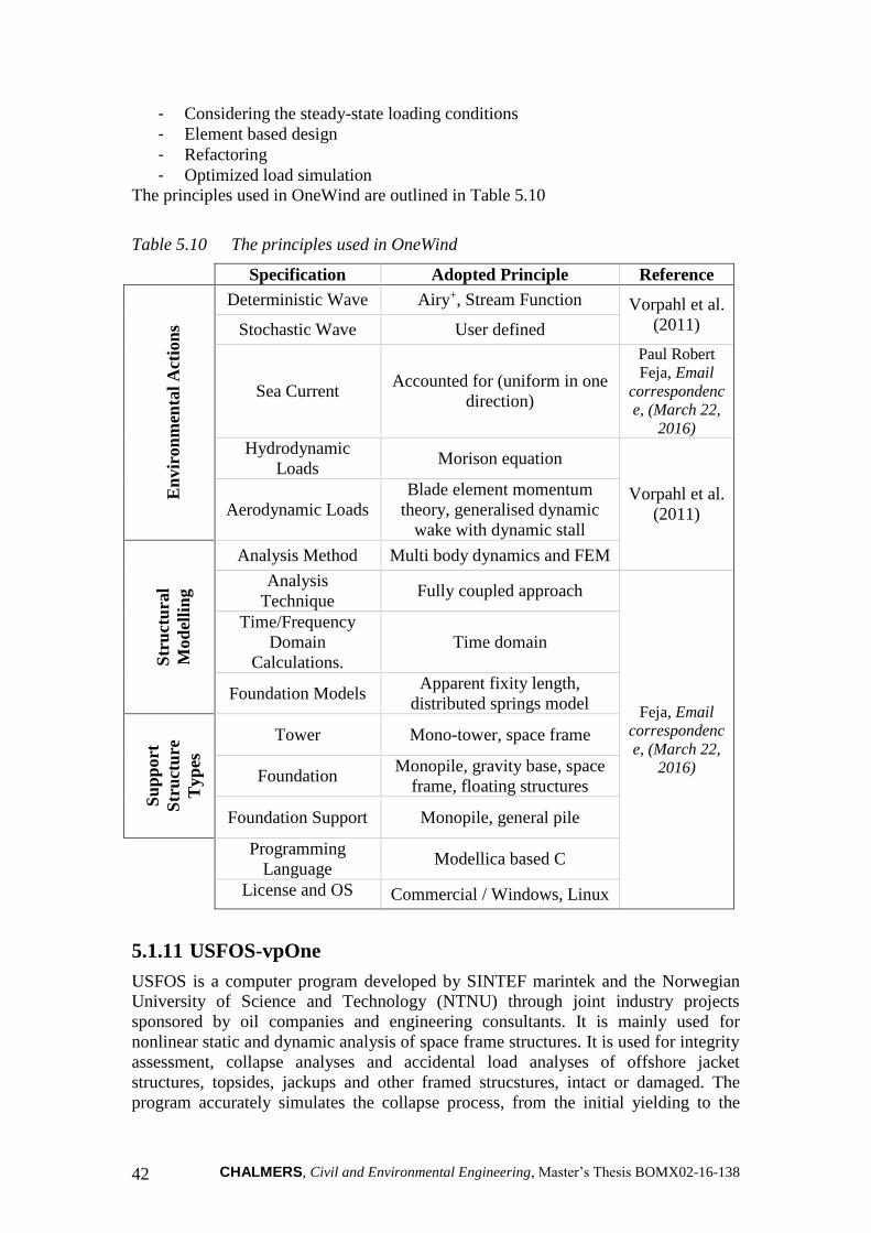
CHALMERS, Civil and Environmental Engineering, Master’s Thesis BOMX02-16-138 42
- Considering the steady-state loading conditions
- Element based design
- Refactoring
- Optimized load simulation
The principles used in OneWind are outlined in Table 5.10
Table 5.10 The principles used in OneWind
Specification Adopted Principle Reference
En
vir
on
men
tal
Act
ion
s
Deterministic Wave Airy+, Stream Function Vorpahl et al.
(2011) Stochastic Wave User defined
Sea Current Accounted for (uniform in one
direction)
Paul Robert
Feja, Email
correspondenc
e, (March 22,
2016)
Hydrodynamic
Loads Morison equation
Vorpahl et al.
(2011) Aerodynamic Loads
Blade element momentum
theory, generalised dynamic
wake with dynamic stall
Str
uct
ura
l
Mod
elli
ng
Analysis Method Multi body dynamics and FEM
Analysis
Technique Fully coupled approach
Feja, Email
correspondenc
e, (March 22,
2016)
Time/Frequency
Domain
Calculations.
Time domain
Foundation Models Apparent fixity length,
distributed springs model
Su
pp
ort
Str
uct
ure
Typ
es
Tower Mono-tower, space frame
Foundation Monopile, gravity base, space
frame, floating structures
Foundation Support Monopile, general pile
Programming
Language Modellica based C
License and OS Commercial / Windows, Linux
5.1.11 USFOS-vpOne
USFOS is a computer program developed by SINTEF marintek and the Norwegian
University of Science and Technology (NTNU) through joint industry projects
sponsored by oil companies and engineering consultants. It is mainly used for
nonlinear static and dynamic analysis of space frame structures. It is used for integrity
assessment, collapse analyses and accidental load analyses of offshore jacket
structures, topsides, jackups and other framed strucstures, intact or damaged. The
program accurately simulates the collapse process, from the initial yielding to the

CHALMERS, Civil and Environmental Engineering, Master’s Thesis BOMX02-16-138 43
formation of a complete collapse mechanism of the structure (SINTEF marintek &
NTNU 2016). Since USFOS has no modules for hydrodynamic and aerodynamic
loadings, there is a need of hydro-servo-aerodynamic simulation code to combine
with. For OWT design, estimated wind and wave loads can be calculated with vpOne,
which is a hydro-servo-aerodynamic tool developed by Virtual Prototyping, and
applied to USFOS. The main principles of USFOS-vpOne are outlined in Table 5.11.
Table 5.11 Specifications of USFOS-vpOne
Specification Adopted Principle Reference
En
vir
on
men
tal
Act
ion
s
Deterministic Wave Airy+, Stream function, Stokes
5th order theory.
Sintef Group
(2010)
Stochastic Wave
Pierson-
Moskowitz/JONSWAP and
Airy+, Grid wave
(Computational fluid
dynamics)
Sea Current Accounted for, represented by
a velocity vector.
Hydrodynamic
Loads Morison equation
Aerodynamic Loads Blade element momentum
theory and dynamic stall
Robertson et
al. (2014)
Str
uct
ura
l M
od
elli
ng
Analysis Method Finite Element Method MARINTEK
(1999)
Analysis
Technique Sequential
Time/Frequency
Domain
Calculations.
Time domain Sintef Group
(2010)
Foundation Models
Distributed springs model
(springs in form of discs
representing soil layers).
MARINTEK
(2009)
Su
pp
ort
Str
uct
ure
Typ
es
Tower Mono-tower, arbitrary space
frame
Foundation Monopile, arbitrary space
frame, floating structures.
Foundation Support Monopile, general pile
Programming
Language UNIX
MARINTEK
(1999)
License and OS Commercial / MS Windows,
Linux, Mac (Usfos n.d.)
5.1.12 SESAM
This is another software package distributed by DNV GL. It is used for designing and
analysing fixed and floating offshore and maritime structures. Modelling, analysis and
results processing are performed in the same graphical user interface. According to
DNV GL (2016), Some of the features of program include:
CHALMERS, Civil and Environmental Engineering, Master’s Thesis BOMX02-16-138 44
- Concept modelling and automated processes that support the need for fast
design iterations.
- Static and dynamic structural analysis incorporating environmental load
calculation (wind, waves, current).
- Analyses are run by the finite element methodology where beams and plates
are all connected together.
- One graphical user interface for modelling, FE analysis and results evaluation.
- One common model used for all phases from initial to final design, as well as
for modifications, repair and life extension.
- Wide range of analyses; code checking load-out, transportation, launching,
installation, fatigue, earthquake, progressive collapse, accidents, explosions.
- It has the capability to import data from other FEA or CAD systems.

CHALMERS, Civil and Environmental Engineering, Master’s Thesis BOMX02-16-138 45
Table 5.12 Specifications of SESAM
Specification Adopted Principle Reference
En
vir
on
men
tal
Act
ion
s Deterministic Wave
Airy+, Stream function, Stokes
theory, Cnoidal and NewWave
theory.
Laurens Alblas,
correspondence,
(May 09, 2016)
Stochastic Wave
Pierson-
Moskowitz/JONSWAP and
Airy, User defined
Sea Current Applicable
Hydrodynamic
Loads
Morison equation (for beam
structures), Wave interaction
and diffraction approach using
panel models (for shell models)
Aerodynamic Loads
Wind turbine loads need to be
calculated via a wind turbine
load calculation tool (e.g.
Bladed, BHawC, HawC2,
Flex5 or other)
Str
uct
ura
l M
od
elli
ng
Analysis Method Multi body dynamics
Analysis
Technique
Fully integrated (Coupled)
analysis, Super-element
analysis and Sequential
analysis
Time/Frequency
Domain
Calculations.
Both frequency and time
domain.
Foundation Models Distributed linear or non-linear
soil springs.
Su
pp
ort
Str
uct
ure
Typ
es
Tower Mono-tower, arbitrary space
frame
Foundation
Monopile, arbitrary space
frame, floating structures,
gravity base
Foundation Support Monopile, general pile,
Programming
Language Fortran, C#, C++ and .NET.
License and OS Commercial or academic /
Windows.
5.2 Comparison of codes
In this section, readers are introduced to the comparison study of the simulation codes
mentioned in Section 5.1. The comparison study of the simulation codes is outlined in
Table 5.13 in terms of the principles adopted to define the environmental actions, the
methods used in structural modelling and the types of support structure that can be
modelled.

46
CH
AL
ME
RS
, Civil a
nd
En
viron
men
tal E
ng
ineerin
g, M
aster`s Th
esis BO
MX
02
-16-1
38
Specification FAST FLEX5 BLADED ADCoS ADAMS & AeroDyn HAWC2 ASHES TURBU
OFFSHORE FOCUS6 One
Wind USFOS SESAM
Deterministic
Wave Airy+ Airy+, ST Airy+, ST Airy+, ST Airy+ Airy+, ST Airy+, ST Airy
Airy+, ST,
FN Airy+, ST
Airy+, ST,
STK
Airy+, ST,
CD, NW,
STK
En
viro
nm
en
tal A
ction
s
Table 5
.13
Com
pariso
n o
f OW
T sim
ula
tion co
des
Stochastic
Wave
PM, UD,
JS, Airy+ PM, UD,
JS, Airy+ PM, JS,UD
CN, Airy+
PM, UD,
JS, Airy+ PM, UD,
JS, Airy+ PM, JS,
Airy+ JS
PM, UD,
JS, Airy PM UD
PM, JS Airy+ CFD
PM, JS Airy+ UD
Sea Current Applicable Sub
Surface Applicable Applicable
Not
Applicable Applicable
Not
Applicable Applicable Applicable Applicable Applicable Applicable
Hydrodynamic
Loads ME, PFT ME ME ME PFT ME ME ME ME, PFT ME ME ME, WI
Aerodynamic
Loads
BEM, GDW+DS
BEM BEM,
GDW+DS BEM,
GDW+DS BEM,
GDW +DS BEM,
GDW +DS BEM+
DS BEM
BEM+
DS BEM,
GDW +DS
BEM+
DS
External
Source
Analysis Method
MA +
MBS MA
MA +
MBS FEM MBS MBS FEM MBS FEM
MBS +
FEM FEM MBS
Str
uctu
ral
Mo
dellin
g
Analysis
Technique FC FC FC SA SA FC FC FC FC FC SA
FC, SA,
SE Time/Freq.
Domain
Calculations TD TD TD, FD TD TD TD TD FD TD TD TD TD, FD
Foundation
Models AF AF AF, DiS
AF,DiS,
UD AF, DiS
AF, DiS,
UD - AF, DiS CS AF, DiS DiS CS, DiS
Tower MT, SF MT MT, SF MT, SF MT, SF MT, SF MT, SF MT MT, SF MT, SF MT, SF MT, SF
Su
pp
ort
Str
uctu
re T
yp
es
Foundation MP,SF,
GB, FL MP
MP, GB,
FL, SF
MP, SF,
GB
MP,SF
GB, FL MP,SF
GB, FL MP, SF,
FL MP
MP, SF,
FL MP, GB,
SF, FL
MP, SF,
FL
MP, GB
SF, FL
Foundation Support
MP, GP
SC, GB MP
MP, GP,
SC MP, GP MP, GP
MP, GP,
UD MP, GP MP
MP, GP,
UD MP, GP MP, GP MP, GP
Programming
Language Fortran
Turbo
Pascal Fortran
VB, C++ Fortran Fortran Fortran
Visual
Studio,C++ Matlab Fortran, C#
Modellica,
C UNIX
Fortran,C
C++, .NET
License and
Operating S.
OS/ Win,
Linux PP/ Win CM / Win
CM/Win,
Linux CM/ Win,
Linux
CM/ Win,
Linux, Mac CM/ Win PP/ Win CM/ Win
CM/ Win,
Linux
CM/ Win,
Linux, Mac CM / Win
AIRY+ -Airy and possible modifications for surface
effects
AF - Apparent Fixity Length BEM - Blade Element
Momentum Theory CD - Cnoidal CFD - Computational Fluid
Dynamics
CN - Constrained New Wave CM - Commercial CS - Coupled springs DS - Dynamic Stall DiS - Distributed Springs FC - Fully Coupled FN - Fenton’s Model FD - Frequency Domain FEM - Finite Element Method
FL - Floating Structure GDW - Generalised Dynamic
Wake GB - Gravity Base Structure GP - General Pile JS - JONSWAP MA - Modal Analysis MBS - Multi Body Dynamic
Analysis
ME - Morison Equations MP - Monopile MT - Mono Tower NW - NewWave OS - Open Source PFT - Potential Flow Theory SA - Sequential Analysis SE - Super Element Analysis SC - Suction Caisson
SF - Space Frame ST - Stream Function STK - Stokes TD - Time Domain UD - User Defined PM - Pierson-Moskowitz PP - Proprietary VB - Visual Basic
WI - Wave Interaction

CHALMERS, Civil and Environmental Engineering, Master’s Thesis BOMX02-16-138 47
6 OWT Design Process
This chapter discusses the procedure of obtaining design loads from site data based on
the guidelines provided by DNV(2010), IEC (2005) and (IEC 2009). The chapter also
focuses on the main design loads considered in the context of the case study in
Chapter 7. The load cases considered in the design are extracted from DNV (2014).
6.1 Design environment loads
6.1.1 Wind loads
The wind climate of a given site is normally described using statistical distributions
which are then used to compute the 10-minute mean wind speed at hub height.
According to DNV (2010), the wind profile against an OWT structure can be obtained
in terms of the 10 minute mean wind speed using the following equation;
0
ln
( ) ( ) 1
ln
z
HU z U H
H
z
(6.1)
)(HU is the 10-minute mean wind speed at a certain height H while )(zU is the sought
mean wind speed at a height z . 0z is the terrain roughness parameter based on Table
2-1 of DNV(2010).
From the site wind climate statistics, extreme wind speed at certain heights are
obtained for a set of expected return periods. Some load cases in DNV (2014) specify
such extreme wind cases instead of the mean.
To include the effects of turbulence in power production and the response of the
structure, the turbulence intensity factor is needed. This parameter is obtained from
the site wind measurements for given heights and also depends on the direction of the
incident wind.
6.1.2 Wave loads
Wave loads are characterised by the wave period and significant wave height.
According to DNV(2010), the significant wave height refers to the average height
(trough to crest) of the highest one-third waves in a given time period.

CHALMERS, Civil and Environmental Engineering, Master’s Thesis BOMX02-16-138 48
Figure 6.1 Statistical wave distribution illustrating the concept of significant wave
height
From field measurements, statistical values of the significant wave height for extreme
wave cases in certain return periods can be obtained.
6.1.3 Wind generated waves
Though waves are also generated through other means, there is no doubt that the wind
contributes most to waves in large water bodies. The role of wind in the generation of
waves continues to be an important subject in oceanographic research to fully
understand the transfer of wind energy into wave energy.
The characteristics of wind generated waves were studied in detail by Bretschneinder
(1964). He devised a number of graphs to estimate the significant wave height and its
associated period at the end of a fetch length for a given wind speed, duration and
fetch (see figure 7.8 in Thomson (1981)). Such graphs also permit determination of
the significant wave characteristics under fetch-limited and duration-limited
conditions, if either the fetch or duration of the wind is insufficient to generated fully
developed seas.
6.1.4 Wind generated current
Loads due to currents can be either wind induced or due to geographic water streams.
From the site measurements, statistical current speed data together with the direction
is needed to satisfy the pertinent load cases specified in DNV (2014). Unless data
indicates otherwise, the wind generated current at still water level may be estimated
as:
0 0wind k U (6.2)
where k ranges from 0.015 to 0.03 and 0U is the 1-hour mean wind speed at 10 m
height DNV (2014).
0
5
10
15
20
25
30
0 2 4 6 8 10 12
Nu
mb
er o
f w
aves
Wave height
Statistical wave distribution
1/3 of waves
Significant
wave height

CHALMERS, Civil and Environmental Engineering, Master’s Thesis BOMX02-16-138 49
Similar to wind and wave loads, statistical values of the current velocities are obtained
from field measurements for certain return periods.
6.2 Design input data for the codes
The input data required for each code prior to modelling and analysing an OWT
structure may vary slightly from one code to another. However, the general
requirements are still maintained since all the codes run on virtually similar theories
and principles (see Chapter 4). In this section, the various specifications required to
analyse an OWT structure are discussed.
6.2.1 Geometry and material properties.
This set of data describes blade, tower and substructure geometry which includes
member sizes, section and material properties. For most codes like Bladed, Ashes and
HAWC2; predefined blades can be used if required. However, if the user requires a
turbine with blades other than those predefined then the entire blade geometry has to
be rigorously modelled following the code’s blade modeller. This is also true for the
tower and substructure, which can be modelled using coordinates that define element
topology. These coordinates represent the structural joints.
6.2.2 Aerodynamic data
The appropriate wind spectrum has to be defined in order to set up the aerodynamic
environment of the OWT, as shown in Section 4.2. Consequently, one has to state the
mean wind speed together with the height at which the wind speed is defined. The air
density, air viscosity, flow inclination and wind direction are also required.
Longitudinal, lateral and vertical intensity factors for turbulence may be required
depending on the complexity of the model.
Where applicable, codes that employ Blade Element Momentum (BEM) theory to
model aerodynamic loads require the user to state the value of the aerodynamic
coefficients. Some go ahead to combine the BEM theory with drag effects in a similar
fashion to Morrison’s equation. In that case, the drag coefficient needs to be provided
for aerodynamic loads.
6.2.3 Hydrodynamic data
Wave characteristics are fundamental when it comes to describing the hydrodynamic
environment of the OWT structure as discussed in Section 4.3. This, however,
depends on the nature of the waves (regular or irregular) and requires that the
appropriate wave type is selected. For deterministic wave models, the wave height
and period have to be specified. The JONSWAP/Pierson Moskowitz function requires
one to define the significant wave height, peak spectral period and peak factor. In
some codes though the user is allowed to define a wave spectrum from scratch. In all
cases, the wave direction is required.
Depending on the hydrodynamic loading model that the code uses, a number of
coefficients need to be specified including the mean water depth. Morison equation
requires the hydrodynamic and drag inertia coefficients.

CHALMERS, Civil and Environmental Engineering, Master’s Thesis BOMX02-16-138 50
The current velocity and type are required as an input in the model. The direction
(angle) at which the current arrives at the OWT has to be defined.
The salinity, temperature, viscosity and density of the water are required since these
bare a direct effect on the flow characteristics.
6.2.4 Initial and boundary conditions
Initial conditions include the initial angular blade rotation speed, the initial structural
orientation and the initial wave profile. The initial wind conditions should be
specified too.
Boundary conditions between different structural parts and at the support should be
specified in order to obtain a whole set of coupled results.
6.2.5 Soil interaction data
Some codes describe the foundation boundary conditions simply as a fixed or pinned
node, while others are capable of presenting a system of soil interaction of the forms
described in Section 4.1.
6.2.6 Computational specifications
This set of input data includes convergence criteria, analysis time step, analysis
method (linear and nonlinear) and the preferred iteration method.
6.2.7 Summary
Table 6.1 summarises the main input data required in order to run an OWT
simulation.
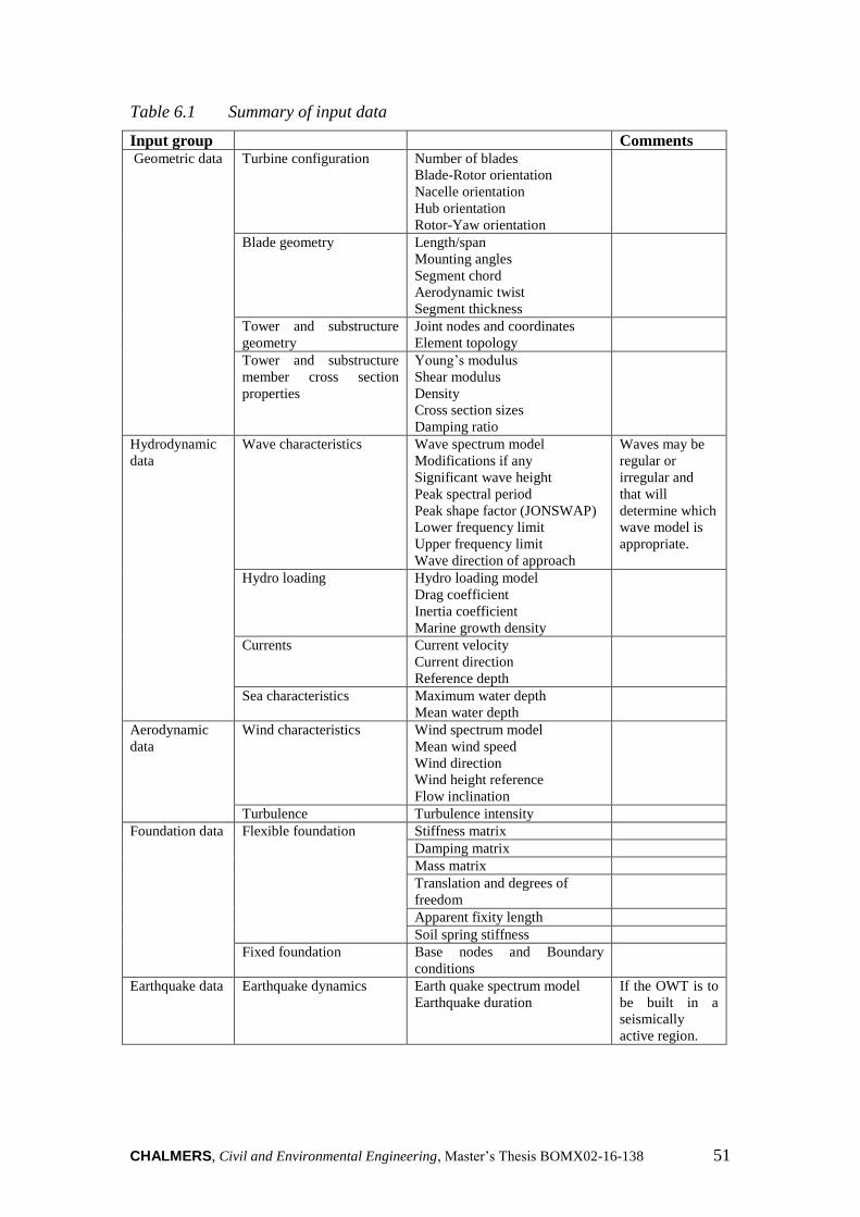
CHALMERS, Civil and Environmental Engineering, Master’s Thesis BOMX02-16-138 51
Table 6.1 Summary of input data
Input group Comments Geometric data Turbine configuration Number of blades
Blade-Rotor orientation
Nacelle orientation
Hub orientation
Rotor-Yaw orientation
Blade geometry Length/span
Mounting angles
Segment chord
Aerodynamic twist
Segment thickness
Tower and substructure
geometry
Joint nodes and coordinates
Element topology
Tower and substructure
member cross section
properties
Young’s modulus
Shear modulus
Density
Cross section sizes
Damping ratio
Hydrodynamic
data
Wave characteristics Wave spectrum model
Modifications if any
Significant wave height
Peak spectral period
Peak shape factor (JONSWAP)
Lower frequency limit
Upper frequency limit
Wave direction of approach
Waves may be
regular or
irregular and
that will
determine which
wave model is
appropriate.
Hydro loading Hydro loading model
Drag coefficient
Inertia coefficient
Marine growth density
Currents Current velocity
Current direction
Reference depth
Sea characteristics Maximum water depth
Mean water depth
Aerodynamic
data
Wind characteristics Wind spectrum model
Mean wind speed
Wind direction
Wind height reference
Flow inclination
Turbulence Turbulence intensity
Foundation data
Flexible foundation
Stiffness matrix
Damping matrix
Mass matrix
Translation and degrees of
freedom
Apparent fixity length
Soil spring stiffness
Fixed foundation Base nodes and Boundary
conditions
Earthquake data Earthquake dynamics Earth quake spectrum model
Earthquake duration
If the OWT is to
be built in a
seismically
active region.

CHALMERS, Civil and Environmental Engineering, Master’s Thesis BOMX02-16-138 52
7 Case Study and Code Comparison
In this chapter, three codes were used to simulate various types of OWT foundations.
The chapter includes a pre-study of the jacket structure used in OC4 and a case study
to compare results of a tripod and a gravity base structure. The results from each code
were used to study the differences and similarities between the codes. In addition, the
wind turbine model (RNA and tower) used in the comparison studies is briefly
discussed in Section 7.2. For more details on this turbine model, the reader is referred
to Jonkman et al. (2009).
7.1 Pre-study
This exercise was done prior to the actual case study with the main purpose of
ensuring familiarity with the software before using them on actual case studies. The
exercise was based on the models and results of the OC4 project. For more details
about OC4 project, readers are referred to Vorpahl et al. (2011).
The same jacket structure studied in OC4 was defined in both FAST and ASHES with
identical tower and turbine configurations. To be consistent with the study, the same
load cases and corresponding initial conditions were defined in both software. The
structural model was assumed to be fixed at the bottom as the one in OC4 project. In
other words, soil-pile interaction was not considered in the model. The results
obtained from the models and OC4 study are shown as follows with related
comments.
7.1.1 Pre-Study with OC4 Load Case 2.1
With this load case, the codes are compared when there is no wind action on the
structure and water stands still. Same conditions were defined and since there were no
horizontal forces acting on the structure only the forces in axial (vertical) direction
were extracted at this phase. The calculated vertical forces at the mudline obtained
from both programs are shown in Figure 7.1.

CHALMERS, Civil and Environmental Engineering, Master’s Thesis BOMX02-16-138 53
Figure 7.1 Vertical force at the mudline from load case 2.1
There is a small difference between the two results, but both results are still in the
range of the results obtained in OC4 studies which is approximately between 15600
and 17200 kN.
7.1.2 Pre-Study with OC4 Load Case 2.3a
In this load case, the attention was given to wave and buoyancy effect. No wind was
defined in the models and waves were modelled considering 6m wave height and 10s
wave period. In this load case, both axial (vertical) and shear force at the mudline
were extracted and compared.
Figure 7.2 Vertical force at the mudline from load case 2.3a
15500
15700
15900
16100
16300
16500
16700
16900
10 20 30 40 50 60
Axi
al F
orc
e (k
N)
Time (s)
Vertical Force at the Mudline from LC-2.1 FAST
ASHES
15000
15200
15400
15600
15800
16000
16200
16400
16600
16800
17000
10 20 30 40 50 60
Axi
al F
orc
e (k
N)
Time (s)
Vertical Force at the Mudline from LC-2.3a FAST
ASHES

CHALMERS, Civil and Environmental Engineering, Master’s Thesis BOMX02-16-138 54
The vertical force results from both analyses show coherence with the results from
OC4. The buoyancy force due to the waves causes the oscillation in the axial force at
the mudline. In OC4, the vertical force results for all simulation codes fluctuate
approximately between 15400 and 17400kN.
Figure 7.3 Fore-aft shear force at mudline from load case 2.3a
The shear force obtained from ASHES is considerably smaller than FAST. The main
reason behind this difference is the additional horizontal force originated from the
interaction between marine growth and wave action. In ASHES, it is not possible to
define marine growth yet, therefore, the shear force at mudline is smaller than FAST
and the rest of the codes studied in OC4. However, both results are quite similar to the
results gotten from OC4 study. Moreover, it can be seen from the results obtained
from both analyses that the ripples around the peaks in the graphs are vanishing with
time due to the fact that the structure reaches the steady-state conditions and follows
the excitation force rather than natural vibration.
7.1.3 Special case of OC4 Load Case 2.3a
This case was created to verify if the marine growth-wave interaction was the actual
reason behind the difference between the fore-aft shear force results as it was stated in
Section 7.1.2. The method followed here was removing the marine growth definition
from FAST and adding the corresponding mass to the structure to get the same
structural mass in both models. In the previous FAST model used in Section 7.1.2, the
marine growth was included in the model to obtain comparable results with OC4
study even though it was not possible to do it in ASHES. In Figure 7.4 and Figure 7.5,
FAST results were calculated without defining the marine growth as described above.
Apart from that, the results shown from ASHES are the same with those in Section
7.1.2.
-1000
-800
-600
-400
-200
0
200
400
600
800
1000
10 20 30 40 50 60
Fo
re-a
ft S
hea
r F
orc
e (k
N)
Time (s)
Fore-aft Shear Force at Mudline from LC-2.3a FAST
ASHES
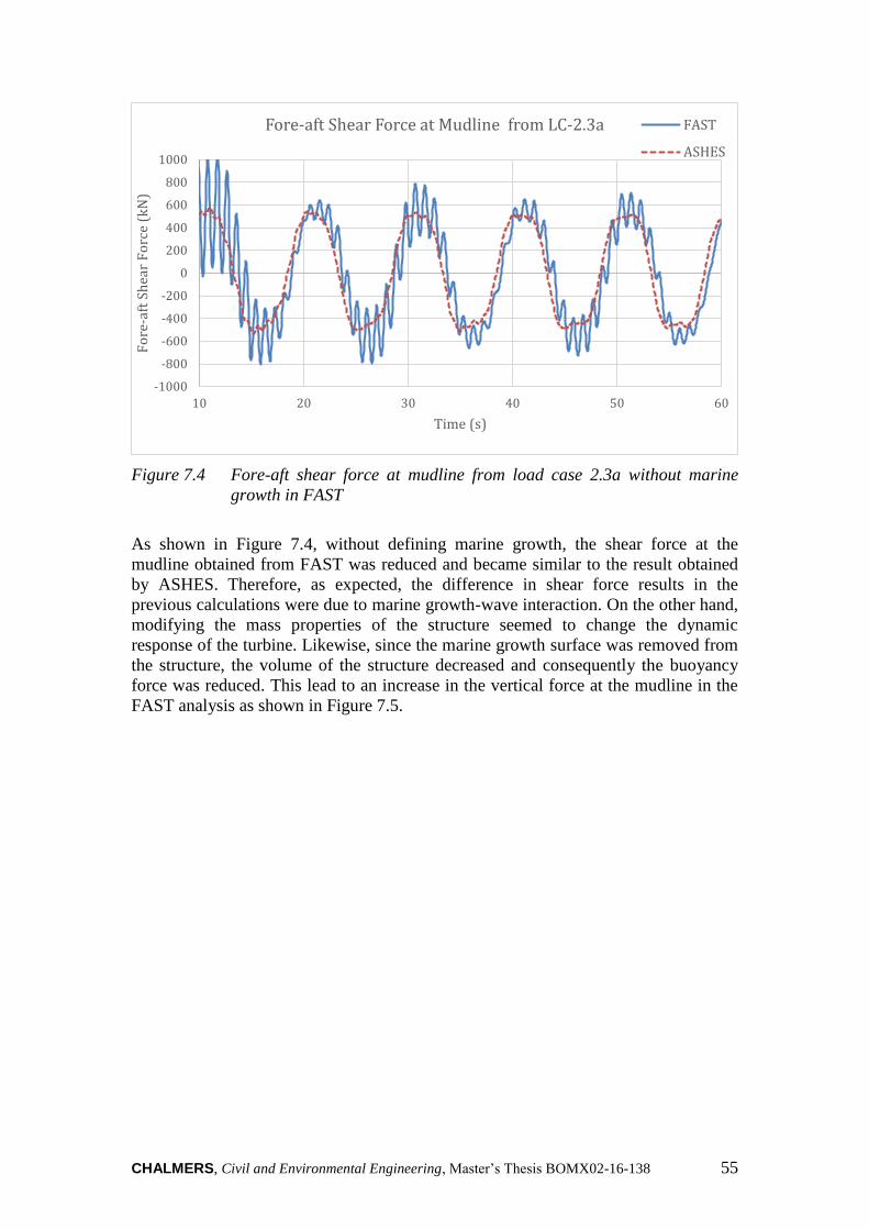
CHALMERS, Civil and Environmental Engineering, Master’s Thesis BOMX02-16-138 55
Figure 7.4 Fore-aft shear force at mudline from load case 2.3a without marine
growth in FAST
As shown in Figure 7.4, without defining marine growth, the shear force at the
mudline obtained from FAST was reduced and became similar to the result obtained
by ASHES. Therefore, as expected, the difference in shear force results in the
previous calculations were due to marine growth-wave interaction. On the other hand,
modifying the mass properties of the structure seemed to change the dynamic
response of the turbine. Likewise, since the marine growth surface was removed from
the structure, the volume of the structure decreased and consequently the buoyancy
force was reduced. This lead to an increase in the vertical force at the mudline in the
FAST analysis as shown in Figure 7.5.
-1000
-800
-600
-400
-200
0
200
400
600
800
1000
10 20 30 40 50 60
Fo
re-a
ft S
hea
r F
orc
e (k
N)
Time (s)
Fore-aft Shear Force at Mudline from LC-2.3a FAST
ASHES

CHALMERS, Civil and Environmental Engineering, Master’s Thesis BOMX02-16-138 56
Figure 7.5 Vertical force at mudline from load case 2.3a without marine growth in
FAST
7.2 RNA and tower definitions used in the studies
7.2.1 NREL 5MW Wind turbine model
This turbine model was developed by the National Renewable Energy Laboratory
(NREL) funded through the U.S Department of Energy (DOE). It features
representative specifications of a typical land and sea-based multi-megawatt turbine
suitable for deployment in deep waters. Because of the cost of offshore support
structures, the NREL decided that a minimum power rating of 5 MW for each turbine
is required to warrant feasibility of an OWT power project.
According to Jonkman et al. (2009), the 5 MW baseline was chosen based on past
successful studies that used similar turbine models and specifications. For instance:
- The scope of the floater concepts for offshore wind turbines was built on 5
MW unit specifications and assumptions (Musial et al. cited in Jonkman et al.
2009).
- The rotor diameter of 128 m featured in unpublished DOE offshore cost
studies, which is a representative blade size of a 5-to-6 MW wind turbine.
- Wind Partnerships for Advanced Component Technology (WindPACT)
considered systems rated up to 5 MW in their studies.
- The conceptual design calculations in the Recommendations for Design of
Offshore Wind Turbines were based on a 5 MW rating turbine.
- A 6 MW rating turbine was used in the Dutch Offshore Wind Energy
Converter (DOWEC) project.
- The largest wind turbine prototypes were each 5 MW rated, at the time the
NREL model was developed.
The gross properties of chosen for the NREL 5 MW baseline wind turbine by
Jonkman et al. (2009) are summarised in Table 7.1.
15000
15500
16000
16500
17000
17500
18000
18500
19000
10 20 30 40 50 60
Axi
al F
orc
e (k
N)
Time (s)
Vertical Force at the Mudline from LC-2.3a FAST
ASHES
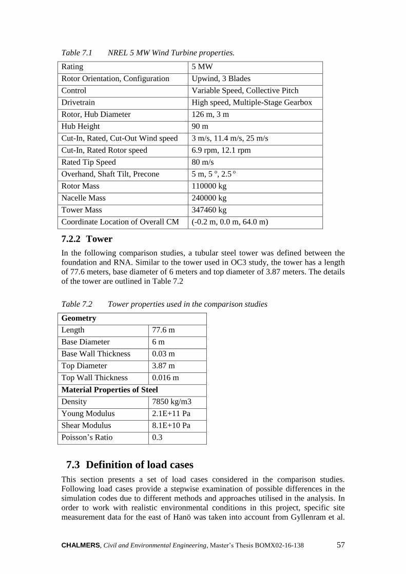
CHALMERS, Civil and Environmental Engineering, Master’s Thesis BOMX02-16-138 57
Table 7.1 NREL 5 MW Wind Turbine properties.
Rating 5 MW
Rotor Orientation, Configuration Upwind, 3 Blades
Control Variable Speed, Collective Pitch
Drivetrain High speed, Multiple-Stage Gearbox
Rotor, Hub Diameter 126 m, 3 m
Hub Height 90 m
Cut-In, Rated, Cut-Out Wind speed 3 m/s, 11.4 m/s, 25 m/s
Cut-In, Rated Rotor speed 6.9 rpm, 12.1 rpm
Rated Tip Speed 80 m/s
Overhand, Shaft Tilt, Precone 5 m, 5 o, 2.5 o
Rotor Mass 110000 kg
Nacelle Mass 240000 kg
Tower Mass 347460 kg
Coordinate Location of Overall CM (-0.2 m, 0.0 m, 64.0 m)
7.2.2 Tower
In the following comparison studies, a tubular steel tower was defined between the
foundation and RNA. Similar to the tower used in OC3 study, the tower has a length
of 77.6 meters, base diameter of 6 meters and top diameter of 3.87 meters. The details
of the tower are outlined in Table 7.2
Table 7.2 Tower properties used in the comparison studies
Geometry
Length 77.6 m
Base Diameter 6 m
Base Wall Thickness 0.03 m
Top Diameter 3.87 m
Top Wall Thickness 0.016 m
Material Properties of Steel
Density 7850 kg/m3
Young Modulus 2.1E+11 Pa
Shear Modulus 8.1E+10 Pa
Poisson’s Ratio 0.3
7.3 Definition of load cases
This section presents a set of load cases considered in the comparison studies.
Following load cases provide a stepwise examination of possible differences in the
simulation codes due to different methods and approaches utilised in the analysis. In
order to work with realistic environmental conditions in this project, specific site
measurement data for the east of Hanö was taken into account from Gyllenram et al.

CHALMERS, Civil and Environmental Engineering, Master’s Thesis BOMX02-16-138 58
(2009) to generate the load cases. The location of the area is shown in Figure 7.6
(Google Maps, 2016). Blekinge Offshore AB, the proprietors of the Blekinge offshore
site, assigned SMHI with a task to measure environmental conditions.
Figure 7.6 The location of the measured area
Load cases considered in the analyses are summarised in Table 7.3.
Table 7.3 Load cases used in comparison studies
Load Case Wind Condition Wave
Condition Current
Water
Level
Load Case 1 No wind No Wave No Current No Water
Load Case 2 No Wind No Wave 50-year Current MWL
Load Case 3 No Wind 50-year Wave No Current MWL
Load Case 4 Mean Wind Speed No Wave No Current MWL
DNV-OS-
J101 (2014)
Load Case
1.1
vin<U10,hub<vout
Wind
generated
specific wave
height
Wind generated
current MWL
DNV-OS-
J101 (2014)
Load Case
6.1c
1.1U10-50-yr 50-year Wave 50-year Current 50-year
sea level

CHALMERS, Civil and Environmental Engineering, Master’s Thesis BOMX02-16-138 59
Load case 1 was meant to check if the geometry and mass definitions of the structure
were defined correctly in the models before proceeding with more complex cases.
Load cases 2 and 3 examine the results of the codes for hydrodynamic loadings.
However, in ASHES it is not yet possible to define sea currents, therefore, only FAST
and FOCUS6 were studied in load case 2. Load case 4 was included in this project to
investigate the structural response of the model to wind loading for each simulation
code. Since the wind turbine is parked under extreme wind conditions, load case 4
accounts for a constant wind load corresponding to the mean wind speed to inspect
the aerodynamic response of the simulation codes including the dynamic effect of the
rotor during power production.
To include standard load cases and inspect the codes with combined environmental
effects, load case 1.1 and 6.1c from DNV (2014) were selected. Load case 1.1 deals
with external loads to which the OWT structure is exposed during power production
which is a typical load case for fatigue analysis. In design phases, DNV prescribes an
investigation of the structural behaviour in several wind loadings from the minimum
wind speed for which the turbine can produce energy to the maximum. However, the
scope of this thesis does not include a structural design, therefore, only the mean wind
speed at hub height was taken into account in this load case. Apart from that, load
case 6.1c was chosen to examine results in extreme conditions for a 50-year return
period.
7.3.1 Environmental effects measured from the site.
The environmental effects used in the comparison study were obtained from the
Blekinge site-investigation report by Gyllenram et al. (2009) of SMHI. They were
used to describe the load cases in Table 7.3 and are summarised in Table 7.4. The sea-
current data shown was obtained from point B (see Figure 7.6) as shown in the
investigation report, since the location of this point satisfied the requirements for
mean water depth. However, the mean sea level in the comparison studies was taken
as 35 and 45 meters in gravity base and tripod structure models respectively instead of
the 25 m planned sea depth by Blekinge Ofshore AB.
Table 7.4 Environmental effects measured from Blekinge offshore site
Environmental condition
Mean sea level 35-45 m
Mean wind speed 8.6 m/s at 70.5m height
Wind generated significant wave
height
1.49 m based on a fetch of approx. 180 km
and the prevailing mean wind speed. See
Figure 7,8 in Thomson (1981)
Wind generated wave period 4.84 s
Wind generated current Estimated using Eq. 6.3. 15.9 cm/s
50-year significant wave height 6.5 m in the north east direction
50-year wave period 7.8 s
50-year wind speed 51.9 m/s at 90 m height
50-year sea Level 35-45 m
50-year current 89 cm/s in the north east direction

CHALMERS, Civil and Environmental Engineering, Master’s Thesis BOMX02-16-138 60
Considering the environmental data shown in Table 7.4, the corresponding load cases
are outlined in Table 7.5.
Table 7.5 Studied load cases according to the environmental data measured from
Blekinge offshore site
Load Case Wind Condition Wave
Condition Current
Water
Level
Load Case 1 - - - -
Load Case 2 - - 0.89 m/s MWL
Load Case 3 - H=6.5 m
T=7.8 s - MWL
Load Case 4 8.79 m/s - - MWL
DNV-OS-
J101 (2014)
Load Case
1.1
8.79 m/s H=1.49 m
T=4.84 s 0.159 m/s MWL
DNV-OS-
J101 (2014)
Load Case
6.1c
57.09 m/s H=6.5 m
T=7.8 s 0.89 m/s
50-year
sea level
7.4 Comparison study for tripod structure
7.4.1 Description of the structure
The support structure used here is a symmetric tripod. The choice of this support
structure was driven by a number of factors ranging from feasibility to technical
aspects. In the third phase of the OC3 project, where a tripod structure was studied
using several simulation codes, the support structure was modelled as bottom fixed
disregarding any soil-pile interaction. Likewise, soil-pile interaction was disregarded
in this project. More details about the OC3 project can be found in Jonkman and
Musial (2010). Since ASHES was not included in the OC3 project, it was decided in
this thesis to study a tripod structure in ASHES along with FOCUS6 and FAST.
The structure has a 45-meter tripod foundation under water and a 10-meter transition
piece that starts at the sea level and connects the tubular tower to the foundation. The
details of the tripod structure are outlined in Table 7.6 and Table 7.7.
Table 7.6 Material properties of tripod structure
Material Properties of Steel
Density 7850 kg/m3
Young Modulus 2.1E+11 Pa
Shear Modulus 8.1E+10 Pa
Poisson’s Ratio 0.3
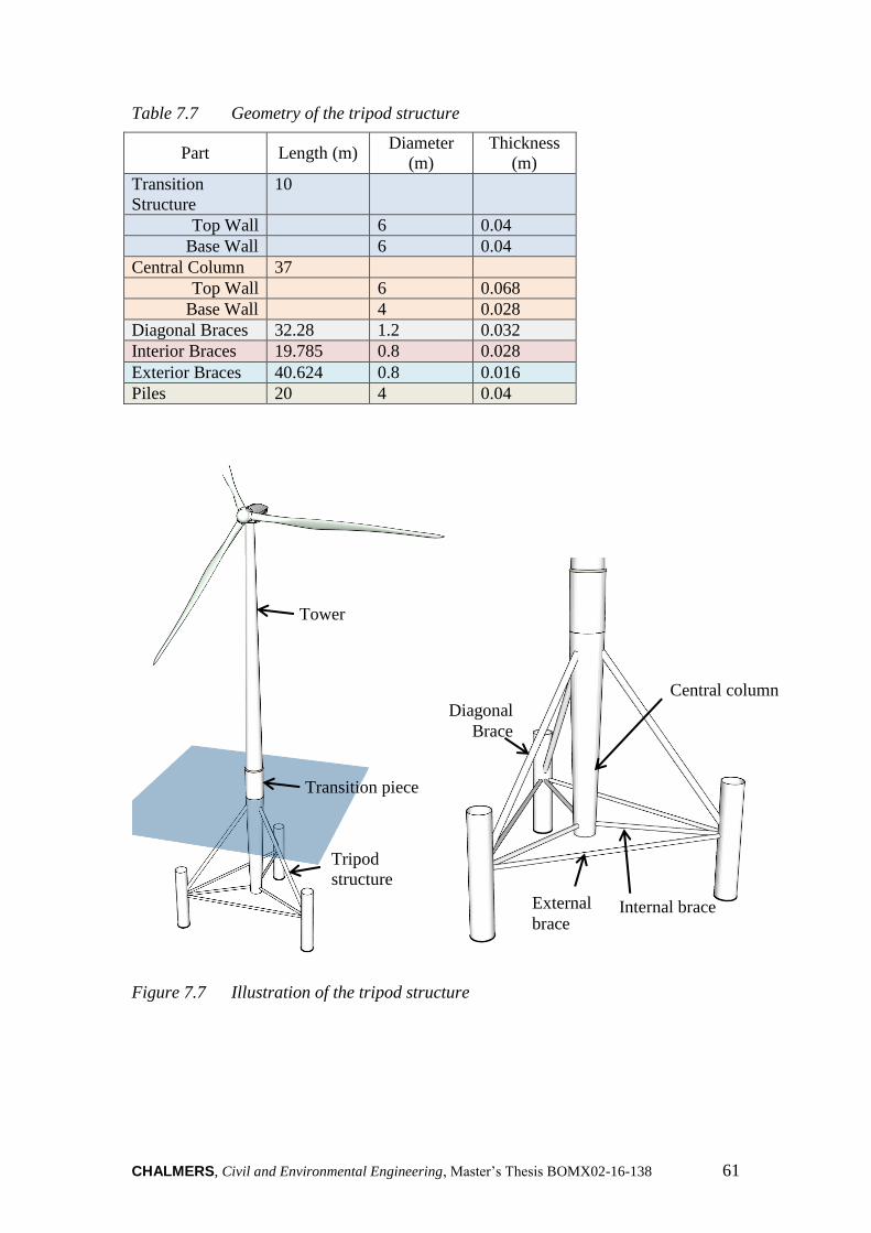
CHALMERS, Civil and Environmental Engineering, Master’s Thesis BOMX02-16-138 61
Table 7.7 Geometry of the tripod structure
Part Length (m) Diameter
(m)
Thickness
(m)
Transition
Structure
10
Top Wall 6 0.04
Base Wall 6 0.04
Central Column 37
Top Wall 6 0.068
Base Wall 4 0.028
Diagonal Braces 32.28 1.2 0.032
Interior Braces 19.785 0.8 0.028
Exterior Braces 40.624 0.8 0.016
Piles 20 4 0.04
Figure 7.7 Illustration of the tripod structure
Tower
Transition piece
Tripod
structure
Central column
External
brace Internal brace
Diagonal
Brace

CHALMERS, Civil and Environmental Engineering, Master’s Thesis BOMX02-16-138 62
7.4.2 Modelling the support structure
In this section, the methods followed to model the tripod structure in the simulation
codes are presented. The tripod structure was modelled in FAST, ASHES and
FOCUS6 in the same way as much as possible to avoid distinctions in the results
coming from the differences in the model itself. In ASHES and FOCUS6, it was not
possible to define a tapered section in a space frame foundation automatically,
therefore, the central column of the tripod structure was divided into 5 members
following the diameter and wall thickness defined in Table 7.7. Even though FAST is
able to define tapered sections, the structure was modelled in the same way in all three
simulation codes as described in the previous sentence.
Moreover, ASHES, is not yet able to define marine growth on the members beneath
the sea level. Since comparing results from two different simulation codes would not
give any hints to observe which one is more precise, the effect of marine growth on
the results was excluded in this comparison. In a similar way, filled members also
cannot be defined in ASHES yet and therefore were disregarded in this study.
The transition piece (the part between the tripod foundation and the tower, see Figure
7.7) in the tripod model is made of steel and defined as a part of the foundation in
FAST and FOCUS6. However, the transition piece in ASHES is very stiff by the
definition of the software itself and cannot be omitted in all space frame foundation
models. Therefore, to obtain the same hub height in all three simulation codes, the
transition piece part of the tripod foundation was subtracted from the model in
ASHES and a stiff transition piece stipulated by the software was added instead. The
effect of this will be discussed comprehensively in the results.
7.4.3 Soil interaction in the model
As mentioned in the description, this study focused on a fixed foundation in which the
soil-pile interaction was ignored. In such a model, the foundation legs were
cantilevered at the mudline.
7.4.4 Results
7.4.4.1 Results from load case 1
It can be seen from Figure 7.8 that there is a very good agreement between the codes.
All codes gave a vertical reaction force slightly greater than 12350 kN in an
acceptable range. Since the tapered sections of the tripod structure were modelled in
the same way for all three codes, it was expected to have very similar results.

CHALMERS, Civil and Environmental Engineering, Master’s Thesis BOMX02-16-138 63
Figure 7.8 Vertical force at mudline for load case 1
7.4.4.2 Results from load case 2
The fore-aft shear force results at the mudline are presented in Figure 7.9. There is a
slight difference in the results even though the same current profile was selected in
both codes but the difference is still acceptable. Additionally, FAST results fluctuate
more compared to FOCUS6 results, but it can also be observed from the diagram that
the response gently tends to reach steady-state.
Figure 7.9 Fore-aft shear force at mudline for load case 2
11000
11200
11400
11600
11800
12000
12200
12400
12600
12800
13000
0 10 20 30 40 50 60
Ver
tica
l F
orc
e (k
N)
Time (s)
Vertical Force at MudlineFAST
ASHES
FOCUS6
0
50
100
150
200
250
300
350
400
450
500
0 10 20 30 40 50 60
Shea
r F
orc
e (k
N)
Time (s)
Fore-Aft Shear Force at Mudline FAST
FOCUS6

CHALMERS, Civil and Environmental Engineering, Master’s Thesis BOMX02-16-138 64
7.4.4.3 Results from load case 3
FAST and FOCUS6 are able to construct wave loads with both Morison Equation and
Potential Flow Theory, however, it is not possible to use Potential Flow Theory in
ASHES. Therefore, to obtain comparable results between codes, only Morison
Equation was used to calculate the wave loads in FAST and FOCUS6 too. Apart from
that, the drag coefficient 𝐶𝑑 and inertia coefficient 𝐶𝑚 in hydrodynamic load
calculations were selected as 1 and 2 respectively.
Altogether, Figure 7.10 shows the fore-aft shear force results at mudline. After taking
a glance at the figure, one can easily observe that there is an incoherence in the
periods of the results from ASHES. However, the difference is only in periods in this
case. The amplitudes from all three codes are around 1750 kN differing by +/- 75 kN
which shows a good agreement between each other. In addition, the results from
FAST initiates with ripples that vanish with time depending on how calculation is
initialised in the code.
Figure 7.10 Fore-aft shear force at mudline for load case 3
7.4.4.4 Results from load case 4
In this load case, BEM theory was used in the calculations with hub loss, tip loss
corrections. Apart from that, the effect of the wind load on the tower was excluded in
these calculations to observe the structural behaviour under wind loads acting only on
the blades and hub. However, this effect was included in the subsequent load cases 5
and 6.
It can be observed from Figure 7.11 that the shear force results from all participant
simulation codes show coherence with each other. The results converge to a shear
force of around 480 kN showing a very good agreement. Still, there is a difference in
the way of load application in the code.
-2500
-2000
-1500
-1000
-500
0
500
1000
1500
2000
2500
0 10 20 30 40 50 60
Shea
r F
orc
e (k
N)
Time (s)
Fore-Aft Shear Force at MudlineFASTASHESFOCUS6

CHALMERS, Civil and Environmental Engineering, Master’s Thesis BOMX02-16-138 65
Figure 7.11 Fore-aft shear force at mudline for load case 4
In the tower top fore-aft deflections (Figure 7.12), FAST and FOCUS6 results show a
good match. FAST result fluctuates about 37.5 cm whereas FOCUS6 result fluctuates
about 38.5 cm. However, ASHES result converges to 33 cm. The main cause of this is
the difference in the transition piece definitions between the codes. As explained in
Section 7.4.2, the transition piece in ASHES was obligatorily modelled as if it was
infinitely stiff, whereas in FAST and FOCUS6 the part was modelled as elastic.
Considering that, a stiffer response in ASHES result was normal to encounter.
Figure 7.12 Tower top fore-aft deflection for load case 4
To avoid the effect of this stiff transition piece definition in ASHES, the height of the
transition piece was reduced to 0.1 meter and the remaining (9.9 meters) part was
0
100
200
300
400
500
600
700
800
900
1000
0 10 20 30 40 50 60
Shea
r F
orc
e (k
N)
Time (s)
Fore-Aft Shear Force at MudlineFASTASHESFOCUS6
-0.1
0
0.1
0.2
0.3
0.4
0.5
0.6
0.7
0.8
0.9
0 10 20 30 40 50 60
Def
lect
ion
(m
)
Time (s)
Tower Fore-Aft Deflection FASTFOCUS6ASHES with 10m TP
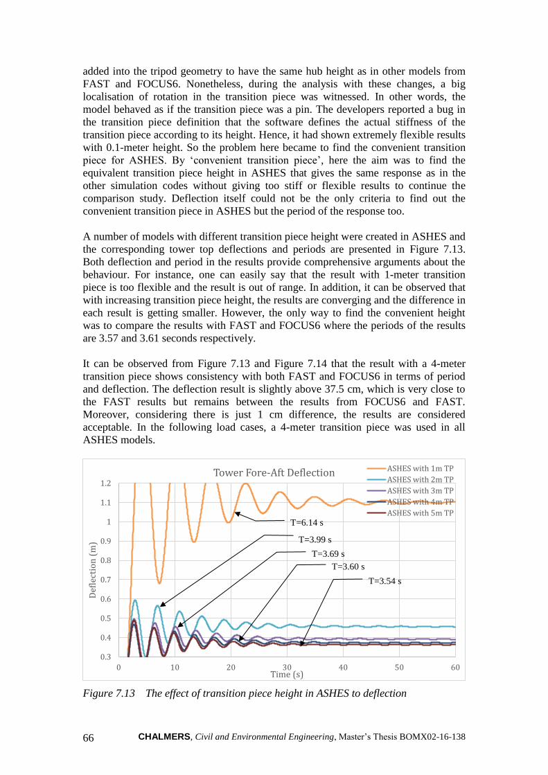
CHALMERS, Civil and Environmental Engineering, Master’s Thesis BOMX02-16-138 66
added into the tripod geometry to have the same hub height as in other models from
FAST and FOCUS6. Nonetheless, during the analysis with these changes, a big
localisation of rotation in the transition piece was witnessed. In other words, the
model behaved as if the transition piece was a pin. The developers reported a bug in
the transition piece definition that the software defines the actual stiffness of the
transition piece according to its height. Hence, it had shown extremely flexible results
with 0.1-meter height. So the problem here became to find the convenient transition
piece for ASHES. By ‘convenient transition piece’, here the aim was to find the
equivalent transition piece height in ASHES that gives the same response as in the
other simulation codes without giving too stiff or flexible results to continue the
comparison study. Deflection itself could not be the only criteria to find out the
convenient transition piece in ASHES but the period of the response too.
A number of models with different transition piece height were created in ASHES and
the corresponding tower top deflections and periods are presented in Figure 7.13.
Both deflection and period in the results provide comprehensive arguments about the
behaviour. For instance, one can easily say that the result with 1-meter transition
piece is too flexible and the result is out of range. In addition, it can be observed that
with increasing transition piece height, the results are converging and the difference in
each result is getting smaller. However, the only way to find the convenient height
was to compare the results with FAST and FOCUS6 where the periods of the results
are 3.57 and 3.61 seconds respectively.
It can be observed from Figure 7.13 and Figure 7.14 that the result with a 4-meter
transition piece shows consistency with both FAST and FOCUS6 in terms of period
and deflection. The deflection result is slightly above 37.5 cm, which is very close to
the FAST results but remains between the results from FOCUS6 and FAST.
Moreover, considering there is just 1 cm difference, the results are considered
acceptable. In the following load cases, a 4-meter transition piece was used in all
ASHES models.
Figure 7.13 The effect of transition piece height in ASHES to deflection
0.3
0.4
0.5
0.6
0.7
0.8
0.9
1
1.1
1.2
0 10 20 30 40 50 60
Def
lect
ion
(m
)
Time (s)
Tower Fore-Aft Deflection ASHES with 1m TP
ASHES with 2m TP
ASHES with 3m TP
ASHES with 4m TP
ASHES with 5m TPT=6.14 s
T=3.99 s
T=3.69 s
T=3.60 s
T=3.54 s

CHALMERS, Civil and Environmental Engineering, Master’s Thesis BOMX02-16-138 67
Figure 7.14 Comparison of ASHES results with FAST and FOCUS6
Furthermore, the fore-aft moment results are presented in Figure 7.15. After steady
state loading, the results are seen to converge to nearly 65000 kNm differing by +/-
1000 kNm. Considering the height of the structure and the difference in shear force,
the results are acceptable.
Figure 7.15 Fore-aft moment at mudline for load case 4
7.4.4.5 Results from DNV load case 1.1
The results for the fore-aft shear force at the mudline for DNV load case 1.1 are
plotted in Figure 7.16. There is a small but visible variation in the shear force
amplitudes: FAST and FOCUS6 show a shear force result going up and down
between nearly +/- 900 kN, but the result from ASHES remains under 850 kN. Apart
0.32
0.34
0.36
0.38
0.4
0.42
0.44
0.46
0.48
15 20 25 30 35 40 45 50 55 60
Def
lect
ion
(m
)
Time (s)
Tower Fore-Aft Deflection FAST
FOCUS6
ASHES with 2m TP
ASHES with 3m TP
ASHES with 4m TP
ASHES with 5m TP
0
20000
40000
60000
80000
100000
120000
140000
160000
0 10 20 30 40 50 60
Mo
men
t (k
Nm
)
Time (s)
Fore-Aft Moment at MudlineFASTASHESFOCUS6
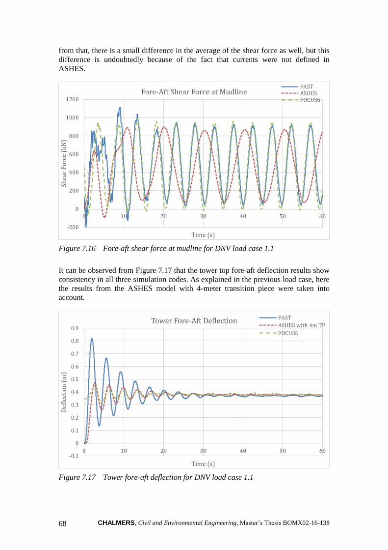
CHALMERS, Civil and Environmental Engineering, Master’s Thesis BOMX02-16-138 68
from that, there is a small difference in the average of the shear force as well, but this
difference is undoubtedly because of the fact that currents were not defined in
ASHES.
Figure 7.16 Fore-aft shear force at mudline for DNV load case 1.1
It can be observed from Figure 7.17 that the tower top fore-aft deflection results show
consistency in all three simulation codes. As explained in the previous load case, here
the results from the ASHES model with 4-meter transition piece were taken into
account.
Figure 7.17 Tower fore-aft deflection for DNV load case 1.1
-200
0
200
400
600
800
1000
1200
0 10 20 30 40 50 60
Shea
r F
orc
e (k
N)
Time (s)
Fore-Aft Shear Force at MudlineFASTASHESFOCUS6
-0.1
0
0.1
0.2
0.3
0.4
0.5
0.6
0.7
0.8
0.9
0 10 20 30 40 50 60
Def
lect
ion
(m
)
Time (s)
Tower Fore-Aft Deflection FAST
ASHES with 4m TP
FOCUS6

CHALMERS, Civil and Environmental Engineering, Master’s Thesis BOMX02-16-138 69
The moment results at the mudline are presented in Figure 7.18. Considering the
different amplitudes in the shear force results, it is ordinary to have bigger difference
in the moment results due to the amplification factor of the moment arm owing to the
structure’s height.
Figure 7.18 Fore-aft moment at mudline for DNV load case 1.1
7.4.4.6 Results from DNV load case 6.1c
The shear force results as shown in Figure 7.19 show consistency at the beginning of
the analysis. However, an unusual instability problem took place in the blades in
ASHES and therefore the ASHES results were truncated to avoid unrealistic extreme
response in the diagram. Apart from that, there is a good agreement between all three
simulation codes.
0
20000
40000
60000
80000
100000
120000
140000
0 10 20 30 40 50 60
Mo
men
t (k
Nm
)
Time (s)
Fore-Aft Moment at MudlineFASTASHESFOCUS6

CHALMERS, Civil and Environmental Engineering, Master’s Thesis BOMX02-16-138 70
Figure 7.19 Fore-aft shear force at mudline for DNV load case 6.1c
The moment results shown in Figure 7.20 have small distinctions, and the ASHES
results were truncated because of the same reason explained before. The irregularities
in the results might be because of the complex extreme loading condition.
Figure 7.20 Fore aft moment at mudline for DNV load case 6.1c
Tower fore-aft deflection results are shown in Figure 7.21. FAST results remain
slightly under the results from ASHES and FOCUS6. In addition, the average of
ASHES results is slightly higher than that of the FOCUS6 results. However, although
it is not possible to see the response for a longer time because of the instability
problem in the blades, the steady-state response of ASHES might be even closer to
the FOCUS6 results.
-1200
-700
-200
300
800
1300
1800
2300
2800
3300
3800
0 10 20 30 40 50 60
Shea
r F
orc
e (k
N)
Time (s)
Fore-Aft Shear Force at MudlineFASTASHESFOCUS6
-25000
25000
75000
125000
175000
0 10 20 30 40 50 60
Mo
men
t (k
Nm
)
Time (s)
Fore-Aft Moment at MudlineFASTASHESFOCUS6

CHALMERS, Civil and Environmental Engineering, Master’s Thesis BOMX02-16-138 71
Figure 7.21 Tower fore aft deflection for DNV load case 6.1c
7.5 Comparison study for the gravity base structure
7.5.1 Description of the structure
The OWT was also analysed with a gravity base foundation, which could be a suitable
solution for the planned offshore wind farm of Blekinge Offshore AB. Furthermore,
its geometry was selected to meet the requirements for the environmental conditions
laid out in the site investigation report by Gyllenram et al. (2009).
Figure 7.22 is an illustration of the OWT tower and its gravity base. In principle, the
gravity base is a hollow reinforced concrete drum with a solid base plate. It is divided
into a conical section that resides below the mean water level and a cylindrical section
which rises up to a height of 10 meters above the mean water level. The steel tower
settles at the top of this cylindrical section. In order to counteract the effect of
buoyancy, it is possible to fill the hollow section of this gravity base with dense fluid
or ballast. The geometry of the base structure is summarised in Table 7.8.
0
0.1
0.2
0.3
0.4
0.5
0.6
0.7
0.8
0 10 20 30 40 50 60
Def
lect
ion
(m
)
Time (s)
Tower Fore-Aft Deflection FAST
ASHES
FOCUS6

CHALMERS, Civil and Environmental Engineering, Master’s Thesis BOMX02-16-138 72
Figure 7.22 Illustration of the gravity base structure
Table 7.8 Geometry of the gravity base structure
Part Height (m) Outer Diameter (m) Thickness
(m)
Base plate 1 25 3.5
Conical section 23
Bottom of cone 18 0.75
Top of cone 6 0.75
Cylindrical section 21 6 0.75
The material properties for the gravity base are summarised in Table 7.9
Table 7.9 Material properties for the gravity base
Material Properties of Concrete
Density 2500 kg/m3
Young Modulus 3.6E+10 Pa
Shear Modulus 2.1E+10 Pa
Poisson’s Ratio 0.2
Tower
Gravity
base
Cylindrical
section
Conical
section
Base plate

CHALMERS, Civil and Environmental Engineering, Master’s Thesis BOMX02-16-138 73
7.5.2 Modelling the support structure
The support structure was modelled element-wise in all of the three simulation codes.
This means that the structure was assumed to be composed of numerous elemental
cylinders that were assembled to form the entire system. In the tapered part of the
structure, the element radius was allowed to decrease sequentially as the foundation
gained height.
In FAST and ASHES, the structure was automatically divided into its sub elements by
virtue of the number of elements defined by the user. FOCUS6 however, could not
carry this out automatically and therefore the elements were described manually.
In practice, the hollow part of the concrete drum is often filled with either water or
suitably dense material. However, here the drum was modelled as unfilled since the
version of ASHES used in this project was not equipped with this capability.
It is often typical to see a transition piece in OWT support structures as extensively
discussed in the tripod model as well as the jacket model. On the other hand, gravity
systems have little regard for a transition piece and therefore the gravity base model in
this project did not include a transition piece. Lastly, similar to the tripod model,
marine growth was disregarded.
7.5.3 Soil interaction in the model
Similar to the tripod model, the gravity base was assumed to be firmly fixed on the
sea bed although in reality there is a reasonable degree of flexibility. This flexibility
was ignored.
7.5.4 Results
7.5.4.1 Results from load case 1
From Figure 7.23, the average weight of the structure at steady state in FAST is seen
to be 32709 kN which is approximately similar to the output from FOCUS6. On the
hand, both the Calfem and ASHES models weighed approximately 32660 kN. This
proximity of results was expected because the model assembly procedure for all the
programs is similar. The tapered part of the structure was divided into the same
number of elements.

CHALMERS, Civil and Environmental Engineering, Master’s Thesis BOMX02-16-138 74
Figure 7.23 Vertical force at the mudline for load case 1
The initial oscillations associated with FAST results originated from the internal
vibrations of the structure prior to reaching steady state conditions. The steady state
internal vibrations are also present in the FOCUS6 result, but cannot be seen due to
the resolution of the graph. However, while the oscillations in FOCUS6 are steady
right from the start of the simulation, the result in ASHES gradually grows from zero
to the maximum steady load without oscillating. This gradual change can only be seen
if the resolution of the graph is increased, as shown in Figure 7.24.
Figure 7.24 ASHES results for the vertical force at the mudline for load case 1
32000
32200
32400
32600
32800
33000
33200
33400
33600
33800
34000
0 10 20 30 40 50 60
Ver
tica
l F
orc
e (k
N)
Time (s)
Vertical Force at Mudline FAST
ASHES
FOCUS6
Matlab&Calfem
0
5000
10000
15000
20000
25000
30000
35000
0 10 20 30 40 50 60
Ver
tica
l F
orc
e (k
N)
Time (s)
Vertical Force at Mudline ASHES

CHALMERS, Civil and Environmental Engineering, Master’s Thesis BOMX02-16-138 75
7.5.4.2 Results from load case 2
On their own, currents produce a relatively small load effect as clearly seen in Figure
7.25. However, there was a difference of about 50kN in the average shear force due to
currents in FOCUS6 and FAST.
Figure 7.25 Fore-Aft shear force at the mudline for load case 2
7.5.4.3 Results from load case 3
Figure 7.26 show resemblance in amplitude for FOCUS6 and FAST. The difference
in phase angle was considered insignificant since it remains consistent. However,
ASHES shows marked differences in both amplitude and phase angle.
0
50
100
150
200
250
300
350
400
450
500
0 10 20 30 40 50 60
Shea
r F
orc
e (k
N)
Time (s)
Fore-Aft Shear Force at Mudline FAST
FOCUS6

CHALMERS, Civil and Environmental Engineering, Master’s Thesis BOMX02-16-138 76
Figure 7.26 Fore-Aft shear force at the mudline, for load case 3
7.5.4.4 Results from load case 4
Load case 4 also presents the results from the Matlab code in addition to FAST,
ASHES and FOCUS6, as a means to verify that the structure was deflecting as
expected.
It can be seen from Figure 7.27 and Figure 7.28, the average deflection results range
from 0.28 m to 0.3m. It was considered acceptable since all the codes produced
results conforming to this range over the entire simulation time.
Figure 7.27 Fore-Aft tower deflection for load case 4
-6000
-4000
-2000
0
2000
4000
6000
0 10 20 30 40 50 60
Shea
r F
orc
e (k
N)
Time (s)
Fore-Aft Shear Force at MudlineFAST
ASHES
FOCUS6
-0.1
0
0.1
0.2
0.3
0.4
0.5
0.6
0.7
0 10 20 30 40 50 60
Def
lect
ion
(m
)
Time (s)
Tower Fore-Aft DeflectionFAST
ASHES
FOCUS6
Matlab&Calfem

CHALMERS, Civil and Environmental Engineering, Master’s Thesis BOMX02-16-138 77
Similar to the deflection, the shear force results in Figure 7.28 showed similarity over
the entire simulation time. The average shear force value according to Figure 7.28 is
480 kN.
Figure 7.28 Fore-Aft Shear force at the mudline for load case 4
The fore-aft bending results in Figure 7.29 followed the same manner as the shear
force results explained before. The average bending moment is seen to be
approximately 60000 kNm according to Figure 7.29.
Figure 7.29 Fore-Aft bending moment at the mudline for load case 4
0
100
200
300
400
500
600
700
800
900
1000
0 10 20 30 40 50 60
Shea
r F
orc
e (k
N)
Time (s)
Fore-Aft Shear Force at Mudline FAST
ASHES
FOCUS6
-20000
0
20000
40000
60000
80000
100000
120000
140000
160000
0 10 20 30 40 50 60
Mo
men
t (k
Nm
)
Time (s)
Fore-aft Moment at MudlineFAST
ASHES
FOCUS6

CHALMERS, Civil and Environmental Engineering, Master’s Thesis BOMX02-16-138 78
7.5.4.5 Results from DNV load case 1.1
Disregarding the initial oscillations shown in the FAST results, the deflection results
shown in Figure 7.30 remain consistent over the entire simulation time. The average
deflection is seen to be approximately 0.3 m.
Figure 7.30 Fore-Aft tower deflection for DNV load case 1.1
The fore-aft shear force results from FAST and FOCUS6 produced some minor
deviation in amplitude. Figure 7.31 shows an approximate difference of 160 kN in
amplitude between FOCUS6 and FAST. However, it is worth noting that this gap in
results remains fairly consistent for most of the simulation.
Figure 7.31 Fore-Aft shear force at the mudline for DNV load case 1.1
-0.1
0
0.1
0.2
0.3
0.4
0.5
0.6
0.7
0 10 20 30 40 50 60
Def
lect
ion
(m
)
Time (s)
Tower Fore-Aft DeflectionFAST
ASHES
FOCUS6
-1500
-1000
-500
0
500
1000
1500
2000
2500
3000
0 10 20 30 40 50 60
Shea
r F
orc
e (k
N)
Time (s)
Fore-Aft Shear Force at MudlineFASTASHESFOCUS6

CHALMERS, Civil and Environmental Engineering, Master’s Thesis BOMX02-16-138 79
The gap exhibited between shear force results for FOCUS6 and FAST is also
exhibited in the fore-aft moment at the mudline. As shown in Figure 7.32, the results
indicate a difference of about 3560 kNm in the amplitude. However, this difference is
seen to remain consistent for the entire simulation time once steady state conditions
are attained. Interestingly, results for ASHES have much the same amplitude as the
FAST results even though, the amplitude in shear force was evidently different.
Figure 7.32 Fore-Aft bending moment at the mudline for DNV load case 1.1
7.5.4.6 Results from DNV load case 6.1c
All ASHES results for DNV load case 6.1c were truncated at 15 seconds, due to
model instability that developed beyond 15 seconds of simulation. This instability
phenomenon was observed in only this load case.
The FAST results are seen to oscillate with higher amplitudes than FOCUS6 and
ASHES. Figure 7.33 shows that these oscillations are dumping out as the simulation
proceeds. It is worth noting that the average deflection seen in the FAST results is not
far off from what FOCUS6 produces, with just a difference of 0.02 m. The average
deflection shown by ASHES results is approximately 0.305 m, which is slightly more
than the FOCUS6 results. Again, this gap remains consistent for a considerable
amount of the simulation time.
-20000
0
20000
40000
60000
80000
100000
120000
140000
160000
180000
0 10 20 30 40 50 60
Mo
men
t (k
Nm
)
Time (s)
Fore-aft Moment at MudlineFAST
ASHES
FOCUS6
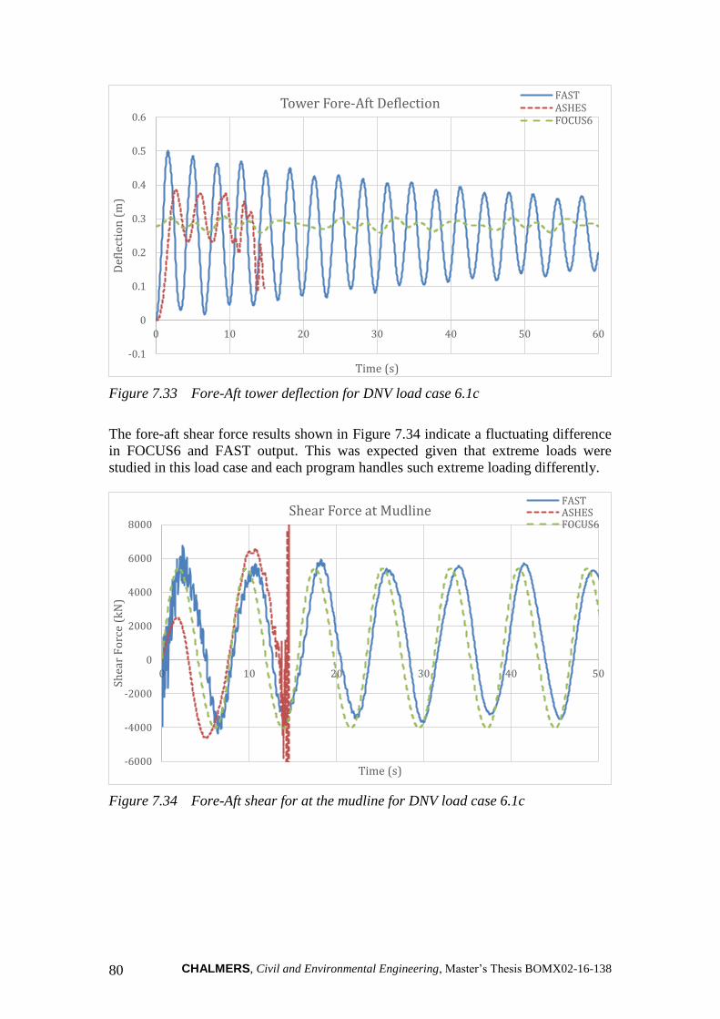
CHALMERS, Civil and Environmental Engineering, Master’s Thesis BOMX02-16-138 80
Figure 7.33 Fore-Aft tower deflection for DNV load case 6.1c
The fore-aft shear force results shown in Figure 7.34 indicate a fluctuating difference
in FOCUS6 and FAST output. This was expected given that extreme loads were
studied in this load case and each program handles such extreme loading differently.
Figure 7.34 Fore-Aft shear for at the mudline for DNV load case 6.1c
-0.1
0
0.1
0.2
0.3
0.4
0.5
0.6
0 10 20 30 40 50 60
Def
lect
ion
(m
)
Time (s)
Tower Fore-Aft DeflectionFASTASHESFOCUS6
-6000
-4000
-2000
0
2000
4000
6000
8000
0 10 20 30 40 50
Shea
r F
orc
e (k
N)
Time (s)
Shear Force at MudlineFASTASHESFOCUS6

CHALMERS, Civil and Environmental Engineering, Master’s Thesis BOMX02-16-138 81
The fore-aft moment results at the mudline shown in Figure 7.35 highlights the
distinctions in the way these programs handle such extreme environmental conditions.
Even though the amplitude seen in the FOCUS6 results is close to that produced by
FAST, the irregularity of the oscillation in the FAST results is very evident. On the
other hand, the FOCUS6 oscillations remain fairly regular. On the contrary, the
irregularity in ASHES oscillations seems to keep growing until the model becomes
unstable. It is fair to say though, that the average fore-aft bending moment results for
FOCUS6 and FAST are similar, approximately 74500 kN. The average for ASHES is
also seen to be close to FAST and FOCUS6.
Figure 7.35 Fore-Aft bending moment at the mudline for DNV load case 6.1c
-50000
0
50000
100000
150000
200000
0 10 20 30 40 50
Mo
men
t (k
Nm
)
Time (s)
Fore-aft Moment at MudlineFASTASHESFOCUS6

CHALMERS, Civil and Environmental Engineering, Master’s Thesis BOMX02-16-138 82
8 Discussion
This chapter discusses the results of the simulations of the tripod and gravity base
support structures and presents the observations made. The differences and
similarities between the code results are discussed in Section 8.1 from one load case
to another, in each case highlighting possible reasons behind discrepancies. In
addition, the results are discussed from a design point of view in Section 8.2. A
summary of the load cases and the respective environmental conditions is shown in
Table 8.1.
Table 8.1 Studied load cases and corresponding environmental condition
Load Case Wind Condition Wave
Condition Current
Water
Level
Load Case 1 - - - -
Load Case 2 - - 0.89 m/s MWL
Load Case 3 - H=6.5 m
T=7.8 s - MWL
Load Case 4 8.79 m/s - - MWL
DNV-OS-
J101 (2014)
Load Case
1.1
8.79 m/s H=1.49 m
T=4.84 s 0.159 m/s MWL
DNV-OS-
J101 (2014)
Load Case
6.1c
57.09 m/s H=6.5 m
T=7.8 s 0.89 m/s
50-year
sea level
As mentioned in Section 7.3, load cases 1 to 4 were only used to consecutively check
the simulation codes in terms of the hydrodynamic and aerodynamic responses hence
they are not typical design load cases. However, from these load cases, it was then
possible to observe the dominant environmental conditions in the results as discussed
later on in Section 8.2.
8.1 Comparison of the simulation codes
A study of the structural weight in load case 1 showed consistent results from all
simulation codes for both the tripod and gravity base models. Furthermore, for the
gravity base system, the results were verified with an additional model created in
Matlab with Calfem toolbox. This confirmed that in both structure types, the model
assembly was correct prior to studying more complex load cases.
Load case 2 was a case of more complexity than load case 1. Again, the agreement
between the simulation codes was evident despite the minor difference in the results.
However, as one might note, this load case did not include results from ASHES
because it is not yet able to model sea currents. In addition, FOCUS6 is limited to the
simple uniform current model whereas FAST is able to describe all possible current
models (Section 4.4). Therefore, to get comparable results between FAST and
FOCUS6, the uniform current model was adopted in FAST even though it was
unrealistic to use it for such deep waters.

CHALMERS, Civil and Environmental Engineering, Master’s Thesis BOMX02-16-138 83
From load case 3, an issue was detected in ASHES: even if the wave period was
changed in the user interface, the software still took a certain time period
(approximately 10.2 seconds) into account. The developers intend to fix this issue in
the next release of the software. In the tripod model, this did not affect the amplitude
of the result. However, there was a considerable increase of the amplitude of the
gravity base result. This was probably attributed to the massive shape of the gravity
base structure; nevertheless, it requires further investigation. The ripples observed in
the results from FAST can be ignored since they are vanishing with time and are
caused by minor start-up transients. Apart from that, the results showed a good
agreement between each simulation code.
The aero-elastic response of the tripod and gravity base structures coming from load
case 4 produced consistent fore-aft shear force results in all three simulation codes.
However, there was a difference in the way the simulation codes apply the
aerodynamic loads at the beginning of the simulation. It was observed that FOCUS6
initialises with a static equilibrium load and therefore the shear force and the tower
deflection start from a certain value. Moreover, in ASHES, the load is ramped up
gradually over the first few steps to minimise the sudden impact of the aerodynamic
load. However, FAST applies the load abruptly at the start and therefore the result
from FAST has very big oscillations at the beginning of the analysis. Nevertheless, all
the codes converge at the same shear force and as mentioned before, start-up
transients can normally be neglected.
Moreover, in load case 4, the tower deflection results from ASHES in the tripod
model were found to be sensitive to the height of the transition piece (see Section
7.4.4.4). The developers aim to correct this in the transition piece definition in the
next release of the program. However, for the gravity base model, the deflection
results were consistent for all simulation codes. Similar to load case 1, these
deflection results were also verified with the Matlab-Calfem model.
DNV load case 1.1 involved typical fatigue conditions. The results of the fore-aft
deflection in both structures showed that the waves and currents have negligible effect
on the deflection of the tower top because of the fact that almost similar results were
obtained with load case 4.
In both structures, the shear force results from DNV load case 1.1 produced a number
of interesting observations. Unlike in load case 3 of the tripod, here the difference in
the wave period between ASHES and the rest caused a difference in the respective
amplitudes of the results. However, it is important to note that the result might be
sensitive to the wave height as well. On the hand, for the gravity base structure, the
difference observed in the amplitudes in load case 3 was also observed in this load
case too.
The moment results for the tripod structure from DNV load case 1.1 were obtained as
expected considering the difference in the shear force results. However, due to the
high moment arm of the geometry, the difference is magnified by the height of the
structure in the moment results. On the contrary, the moment results for the gravity
base were unexpected in comparison to the analogous shear force results. Although,
the amplitude of the shear force results from ASHES was higher than the other

CHALMERS, Civil and Environmental Engineering, Master’s Thesis BOMX02-16-138 84
results, the corresponding moment amplitude from ASHES turned out to be lower.
This might be because of the shape of the gravity base foundation though.
The extremities associated with DNV load case 6.1c resulted into model instabilities
in the blades of the ASHES model for both structures. After a point, the blades
showed unrealistic blade deformations which resulted into an unrealistic structural
response. The developers were made aware of this issue and therefore probable fixes
can be expected in the coming versions. Beside the instability and the wave period
issues in ASHES, the shear force results from all three show consistent agreement.
The moment results from FAST showed more irregularity at the beginning of the
simulation but the behaviour became more regular with time. However, FOCUS6
results did not show a noticeable change with time because of the principle it adopts
to apply the steady-state load at the beginning of the analysis as explained earlier on.
Since ASHES results were truncated because of the instability issue, it was not
possible to check possible irregularities in the results.
Prior to the blade instability, the ASHES deflection results were very similar to those
seen from FOCUS6 in both structures. However, there was a slight difference seen in
the FAST results. In terms of oscillation, the FAST results showed more resilience
against the damping effects that were observed in the previous load cases. This might
be due to the high wind speed, which eventually undermined all possible damping in
the structure.
8.2 Discussion of the results from a design vantage point
As discussed in the Section 2.4, wind turbines are highly dynamic structures which
suffer from both cyclic and extreme loading conditions. Therefore, there are two main
challenges in OWT foundation design namely, fatigue limits and ultimate limits. It is
worth noting that the engineer should also consider serviceability limits in the design.
Hence, this section aims at discussing the results of this study from the design point of
view.
Fatigue design is not only governed by the amplitude of the result but also the number
of load cycles. This implies that the dominant loads in fatigue design are those
responsible for the oscillations in the results. From the results of this thesis project,
this seemed to be mainly due to the waves. However, it is important to remember that
only constant wind action was considered in this thesis. For instance, Figure 7.10, that
represents the shear force results from load case 3, shows considerably big
oscillations from a negative point to a positive one with a mean shear of zero.
However, the shear force profiles due to the currents and wind oscillate about a
certain value without changing the signs as seen in Figure 7.9 and Figure 7.11. The
oscillations here were seen to be less pronounced than those from the waves.
Although one can argue that the reason for this might be because of the steady wind
and current loads, the possibility is very high that even with cyclic wind loading the
magnitude of the oscillations does not exceed that from waves. For that reason, waves
were deemed to be the dominant environmental factor in fatigue design. It should also
be noted that the cyclic behaviour of moment results also has to be considered in
fatigue design, not just the shear.

CHALMERS, Civil and Environmental Engineering, Master’s Thesis BOMX02-16-138 85
Design for ultimate limits on the other hand is only dependent on the magnitude of the
results. In fact, ultimate limit design considers the external loads on the structure in
terms of axial force, shear force and moment respectively.
The dominating load for shear force response at the mudline in ultimate limit state is
highly dependent on the geometry of the structure and specific environmental
conditions. From Figure 7.10, it can be seen that the maximum shear force value due
to the waves is considerably larger than the value due to the currents as shown in
Figure 7.9. In addition, one can also see that the shear force due to the wind as shown
in Figure 7.11 is considerably low compared to that from the waves. However, the
wind speed used to obtain the results shown in Figure 7.11 was the mean value.
Therefore, it is possible that wind can dominate the design if higher wind speeds are
applied.
The dominating load for the moment at the mudline in ultimate limit state is also
highly dependent on the geometry of the structure as well as the environmental
conditions. Although, there is a considerable correlation between shear force and
moment, the leverage of the loads also has a big effect on the moment results. Similar
to the shear response, waves again cause oscillations in the moment results about a
mean value of zero, whereas wind results have small oscillations about a certain
value. For instance, it can be observed from Figure 7.15 for load case 4 and Figure
7.18 for DNV load case 1.1 that the mean values of the moment results are the same,
the only difference being the oscillations in Figure 7.18. Therefore, one can argue that
the wind dictates the average moment whereas the waves dictate the amplitude of the
moment oscillations. In this case, wind governs the moment results. However,
generally it is hard to presume the dominant environmental action for moment results,
since the leverage of the wind action to the base is dependent on the height of the
structure.
The design of the structure in serviceability limit state depends on vibrations and
deformations of the structure. In this project however, only tower top deflection
response was studied in different load cases, not the vibration. In addition, there is no
big difference in the tower top deflection results shown in Figure 7.15 and Figure 7.17
for load case 4 and DNV load case 1.1 respectively, even though the latter case
includes the waves and currents yet the former case has only the wind. This implies
that the deflection at tower top is mainly due to the wind. However, when it comes to
vibration, a steady cyclic load may cause a considerable effect on the serviceability.
Hence, the wave action might dominate the serviceability limits in vibration, of course
the dynamic effects of the wind on vibration (such as dynamic stall) are ignored.
In summary, considering the environmental data and the geometry of the structures
studied in this project, the dominating actions varied for different design
requirements. For instance, waves had a dominant effect in the shear force results at
the mudline compared to the rest. Moreover, due to the cyclic nature of the wave
loads, waves were deemed to be the determining environmental action in fatigue
design and vibrations. On the other hand, wind had a considerable effect on the tower
top deflection and the moment results at the mudline. Currents however, had a little
effect on shear and moment results at the mudline compared to waves and wind. They
merely amplified the shear and moment results.

CHALMERS, Civil and Environmental Engineering, Master’s Thesis BOMX02-16-138 86
9 Conclusion and Future Recommendations
9.1 Conclusion
There are numerous foundation solutions for offshore wind turbines (OWTs) as
revealed by the literature study conducted. These solutions are specific depending on
ground conditions, water depth and other environmental situations. The literature
study also introduced the various principles, methods and load models used in OWT
design. Past literature showed that extensive research has been conducted to develop
OWT simulation codes. From this, one can observe that some simulation codes are
more advanced than the others in terms of being able to describe complex foundation
types and loads. This provided a proper basis for the classification of OWT simulation
codes which outlines the similar and different principles adopted by each code.
Some simulation codes were examined through case studies with two different
foundation structures, including tripod and gravity base to practically establish their
capabilities and limitations. These case studies revealed that the codes differ in
various ways, for instance: mode of modelling the structure, way of describing
environmental loads and analysing models. In addition, the simulation codes showed
variety in the application of the environmental loads, which eventually affect the
response of the structural model. One should note however that the differences also
might depend on the type of the foundation being modelled.
Comparison of different results indicated that a limitation of a code to model a given
environmental condition may result into a number of variations in the output. For
instance, a limitation in the way a code models hydrodynamic loads may result into a
variation in the shear force results which at the same time affects the moment results
at the base. In fact, the code limitations seen in this project were easily detected only
because comparisons were made between codes.
In general terms, there was a good agreement between the results from the simulation
codes and one might be driven to conclude that all simulation codes produce similar
results. However, this would be an over simplified judgement given that only three
simulation codes were studied in this project. A better conclusion may be drawn if
more codes were to be studied. In specific terms though, the differences seen between
the codes varied between different load cases as discussed in Section 8.1. For
instance, the relatively simple load cases (load case 1 to 4) did not show pronounced
differences in the code results, however, the more complex load cases (DNV load
case 6.1c) brought out more marked variations.
Simulation code development has evolved over many years to include new demands
in foundation types, modelling procedure and overall user friendliness. Currently, all
codes are at different stages of development and therefore have different levels of
capabilities. For instance, FAST has very developed load models, turbine control
modules and ability to describe complex structures. FOCUS6 on the other hand, has
advanced load case definition modules which might be very helpful in the design
process. For ASHES, the well-developed user interface makes the modelling process
and result extraction considerably easy. A conclusion is that further development in
the future versions of these simulation codes will only serve to improve the process of
OWT simulation and design by allowing for more realistic model definitions.

CHALMERS, Civil and Environmental Engineering, Master’s Thesis BOMX02-16-138 87
All in all, this project showed that the choice of the simulation code might be
dependent on the type of foundation structure to be designed. Moreover, the study
proved that the environmental conditions also play an important role in the selection
of suitable simulation codes for a given project. For instance, one might look at how
the type of structure depends on the water depth which then defines the theory
appropriate to calculate the hydrodynamic loads acting on the structure. Therefore, it
is important to assess the suitability and capability of the simulation code to be used
before modelling the structure.
9.2 Future recommendations
In this project, due to a restricted timeline, only three simulation codes were studied in
detail. Nonetheless, including more simulation codes with different theories and
principles adopted would bring more interesting discussions. For instance, comparing
simulation codes employing Morison Equations and Potential Flow Theory could give
good arguments not only regarding the choice of simulation codes but also of the
theories used.
Because of the same reason as mentioned above, design aspects of the simulation
codes were not studied in this project. To exemplify, the supported design codes in
terms of load combinations, meeting the modelling requirements specified in the
codes of practice etc. Hence, examining the simulation codes considering the
requirements in the codes of practice would add a different point of view to the
assessment.
Apart from that, only the fixed foundation model was used in all comparison studies.
It would be very interesting to examine the simulation codes for such models with
flexible foundations as well as comparing different flexible foundation models in
different simulation codes.
In addition, the results of this project may open many new horizons for possible future
studies. For instance, the difference in wave period in load case 3 only affects the
shear force results in the gravity base model, but not in the tripod model. The reason
behind this might be the bold diameter or the considerable conical shape of the gravity
base foundation. One way to examine this could be by studying the same load case
with a straight monopile foundation in all three (or more) simulation codes starting
with a considerably tiny section and comparing the results for every increment in the
diameter of the section. According to the response one can bring good arguments such
as: if the shear forces would not show differences in big-sized monopile foundations,
then one can argue that the variation that occurred in this study was because of the
shape of the gravity base foundation and may lead to deep discussions of the
application of the principle adopted in hydrodynamic loading.

CHALMERS, Civil and Environmental Engineering, Master’s Thesis BOMX02-16-138 88
10 References
4C Offshore LTD, 2016. Monopiles Support Structures. Available at:
http://www.4coffshore.com/windfarms/monopiles-support-structures-aid4.html
[Accessed February 11, 2016].
Abhinav, K.A. & Saha, N., 2015. Dynamic analysis of an offshore wind turbine
including soil effects. Procedia Engineering, 116(1), pp.32–39. Available at:
http://dx.doi.org/10.1016/j.proeng.2015.08.261.
Airy, G.B., 1845. Tides and Waves. , pp.241 – 396.
Andrew, S.E. & Todd, R.D., 1996. ADAMS_WT Advanced Development-Version
1_4 and Beyond. , pp.1–11.
Anon, 2016. OneWind. Available at: http://www.onewind.de/OneWindStudent.html
[Accessed April 4, 2016].
API, 2007. Recommended Practice for Planning , Designing and Constructing Fixed
Offshore Platforms — Working Stress Design. Api Recommended Practice, 24-
WSD(December 2000), p.242. Available at:
http://scholar.google.com/scholar?hl=en&btnG=Search&q=intitle:Recommende
d+Practice+for+planning,+designing+and+constructing+fixed+Offshore+Platfor
ms+-+Working+stress+design#0.
Bai, Y. & Jin, W.-L., 2016. Loads and Dynamic Response for Offshore Structures,
Available at:
http://linkinghub.elsevier.com/retrieve/pii/B9780080999975000071.
Bertrand, Y.A., 2002. Middelgrunden offshore wind farm, off the coast of
Copenhagen, Denmark (55°41’ N, 12°40’ E).
Bhattacharya, S., 2014. Challenges in Design of Foundations for Offshore Wind
Turbines. Engineering & Technology Reference, pp.1–9. Available at:
http://digital-library.theiet.org/content/reference/10.1049/etr.2014.0041.
Bretschneinder, C.L., 1964. Generation of Waves by Wind State of the Art.
International Summer Course Lunteren, p.160.
Cassidy, M.J., Taylor, R.E. & Houlsby, G.T., 2001. Analysis of jack-up units using a
Constrained New Wave methodology. Applied Ocean Research, 23, pp.pp. 221–
234.
Crampsie, S., 2014. Offshore windfarms stretch manufacturing supply chains.
Available at: http://eandt.theiet.org/magazine/2014/05/windfarm-
foundations.cfm [Accessed February 25, 2016].
D.Winkelaar, 1992. Program for Three-Dimensional Wind Simulation. , (December),
pp.1–76.
Dean, R.G., 1965. Stream function representation of nonlinear ocean waves. Journal
of Geophysical Research, 70(18), pp.4561–72.
Det Norske Veritas, 2014. Dnv-Os-J101. Design of offshore wind turbine structures,
(June).
DNV, 2010. Environmental Conditions and Environmental Loads October 2010. ,
(October). Available at: http://www.dnv.com.
DNV GL, 2014a. Bladed Theory Manual. , Version 4.(1), pp.1–134.
DNV GL, 2014b. Bladed User Manual. , Version 4.(1), pp.1–209.
DNV GL, 2016. No Title. , p.1.
Eecen, P.., 2003. Wind Waves: Forces due to waves on offshore wind turbines. ,
(September), p.45.
El-Reedy, M.A., 2012. Chapter 2 – Offshore Structure Loads and Strength, Available
at: http://www.sciencedirect.com/science/article/pii/B978012385475900002X.

CHALMERS, Civil and Environmental Engineering, Master’s Thesis BOMX02-16-138 89
van Engelen, T.G. & Braam, H., 2004. TURBU Offshore, computer program for
frequency-domain analysis of horizontal-axis offshore wind turbines -
Implementation. , (September).
Fenton, J.D., 1988. The numerical solution of steady water wave problems.
Computers and Geosciences, 14(3), pp.357–368.
Gyllenram, W., Lindahl, S. & Lindberg, A., 2009. Designunderlag havsbaserad
vindkraft , Hanöbukten.
Hansen, a C. & Laino, D.J., 2002. USER ’ S GUIDE to the Wind Turbine
Aerodynamics Computer Software AeroDyn. , pp.1–60.
Hasselmann, K. et al., 1973. Measurements of Wind-Wave Growth and Swell Decay
during the Joint North Sea Wave Project (JONSWAP). Ergnzungsheft zur
Deutschen Hydrographischen Zeitschrift Reihe, A(8)(8 0), p.p.95.
Henderson, A.R., Zaaijer, M.B. & Camp, T.R., 2003. Hydrodynamic Loading on
Offshore Wind Turbines. Theory Of Ordered Sets And Its Applications, 2(April),
pp.1–15. Available at:
http://www.lr.tudelft.nl/fileadmin/Faculteit/LR/Organisatie/Afdelingen_en_Leers
toelen/Afdeling_AEWE/Wind_Energy/Research/Publications/Publications_2003
/doc/Zaaijer_OWEMES2003_Hydro.pdf.
Hillmer, B. et al., 2007. Aerodynamic and Structural Design of MultiMW Wind
Turbine Blades beyond 5MW. Journal of Physics: Conference Series, 75,
p.012002.
IEC, 2005. IEC 61400-1 Wind Turbines - Part 1: Design requirements. Iec 61400,
2005, pp.1–92. Available at: http://homes.civil.aau.dk/rrp/BM/BM8/r.pdf.
IEC, 2009. International Standard IEC 61400-3 Wind turbines - Part 3: Design
requirements for offshore wind turbines.
Ingram, G., 2011. Wind Turbine Blade Analysis using the Blade Element Momentum
Method. Version 1.1. October, (c), pp.1–21.
J.M. Jonkman, G.J. Hayman, B.J. Jonkman, R.R.D., AeroDyn v15 User’s Guide and
Theory Manual.
Jonkman, B. & Jonkman, J., 2015. FAST v8.12.00a-bjj. , pp.1–42.
Jonkman, J. et al., 2009. Definition of a 5-MW reference wind turbine for offshore
system development. Contract, (February), pp.1–75. Available at: http://tethys-
development.pnnl.gov/sites/default/files/publications/Jonkman_et_al_2009.pdf.
Jonkman, J. & Musial, W., 2010. Offshore code comparison collaboration (OC3) for
IEA task 23 offshore wind technology and deployment. Contract,
303(December), pp.275–3000.
Jonkman, J.M. & Buhl, M.L.J., 2005. FAST User’s Guide. Acta Psychiatrica
Scandinavica, 123(6), pp.407–8. Available at:
http://www.ncbi.nlm.nih.gov/pubmed/21564034.
Jonkman, J.M., Robertson, A.N. & Hayman, G.J., HydroDyn User ’ s Guide and
Theory Manual HydroDyn User ’ s Guide and Theory Manual.
Kaiser, M.J. & Snyder, B.F., 2012. Offshore Wind Energy Cost Modeling -
Installation and Decommissioning. Offshore Wind Energy Cost Modeling.
Available at: http://www.springerlink.com/index/10.1007/978-1-4471-2488-7.
Knowledge Centre WMC, 2016. WMC FOCUS6. Available at:
https://www.wmc.eu/focus6.php [Accessed February 24, 2016].
Larsen, T.J. & Hansen, A.M., 2007. How 2 HAWC2 , the user ’ s manual, Risø
National Laboratory, Technical University of Denmark.
Lindenburg, C., 2005. PHATAS Release “NOV-2003” and “APR-2005” USER’S
MANUAL. , (May).

CHALMERS, Civil and Environmental Engineering, Master’s Thesis BOMX02-16-138 90
Lindenburg, C. & Holierhoek, J.G., 2013. Blademode v2.2 : User Manual. , pp.1–136.
Lucas, C. & Guedes Soares, C., 2015. On the modelling of swell spectra. Ocean
Engineering, 108, pp.749–759. Available at:
http://dx.doi.org/10.1016/j.oceaneng.2015.08.017.
Malhotra, S., 2010. Selection , Design and Construction of Offshore Wind Turbine
Foundations.
MARINTEK, 2009. Modelling of piles in USFOS. , pp.1–15. Available at:
http://www.usfos.no/manuals/usfos/users/documents/Modelling_of_Piles.pdf.
MARINTEK, 1999a. USFOS User’s Manual - Program Concepts. , pp.1–4. Available
at: http://www.usfos.no/manuals/usfos/users/documents/Usfos_UM_02.pdf.
MARINTEK, 1999b. USFOS User’s Manual - Program Concepts. , pp.1–4.
Matha, D. et al., 2010. Model Development and Loads Analysis of a Wind Turbine on
a Floating Offshore Tension Leg Platform. European Offshore Wind Conference,
(February), pp.1–10. Available at: http://www.nrel.gov/docs/fy10osti/46725.pdf.
Le Mehaute, B., 1976. An Introduction to Hydrodynamics and Water waves, New
York: Springer Science+ Business Media New York.
Modelica-Association, 2012. Modelica® -A Unified Object-Oriented Language for
Systems Modeling Language Specification Version 3.3. Available at:
http://www.modelica.org/.
Moriarty, P.J. & Hansen, a C., 2005. AeroDyn Theory Manual. Renewable Energy,
15(January), pp.500–36313. Available at:
http://www.nrel.gov/docs/fy05osti/36881.pdf.
Passon, P. & Branner, K., 2013. Load calculation methods for offshore wind turbine
foundations. Ships and Offshore Structures, 5302(May 2014), pp.1–17.
Available at:
http://www.tandfonline.com/doi/abs/10.1080/17445302.2013.820108.
Passon, P. & Kühn, M., 2005. State-of-the-art and development needs of simulation
codes for offshore wind turbines. Copenhagen Offshore Wind 2005 Conference
and …, pp.1–12. Available at:
http://www.ieawind.org/task_23/Subtask_2S_docs/PPT_Risoe/Copenhagen_200
5-
State_of_the_art_and_development_needs_of_simulation_codes_for_offshore_w
ind_turbines.pdf.
Peeringa, J.M., 2013. CurrentROWS manual: Random linear Ocean Waves
Simulation on a steady uniform current. , (November), pp.1–49.
Peeringa, J.M., 2005. Stream Function program user manual. , (February).
Pierson, W.J.J. & Moskowitz, L., 1964. A Proposed Spectral Form for Fully
Developed Wind Seas Based on the Similarity Theory of S. A. Kitaigorodskii.
Journal of Geophysical Research, 69(24), pp.5181–5190. Available at:
http://adsabs.harvard.edu/cgi-bin/nph-
data_query?bibcode=1964JGR....69.5181P&link_type=EJOURNAL\npapers2://
publication/doi/10.1029/JZ069i024p05181.
Ramachandran, K. et al., 2013. A Numerical Model for a Floating TLP Wind Turbine
A numerical model for a floating TLP wind turbine Department of Wind Energy
Technical University of Denmark.
Robertson, A., Jonkman, J. & Musial, W., 2014. IEA Wind Task 30 Offshore Code
Comparison Collaboration Continued - Final Management Report.
Savenije, F. & Peeringa, J., 2009. Aero-elastic simulation of offshore wind turbines in
the frequency domain. Ecnnl. Available at:
http://www.ecn.nl/docs/library/report/2009/e09060.pdf.

CHALMERS, Civil and Environmental Engineering, Master’s Thesis BOMX02-16-138 91
Simis, 2015. User Manual ASHES 2.1.
Sintef Group, 2010. USFOS Hydrodynamics. , pp.1–95. Available at:
http://usfos.no/manuals/usfos/theory/documents/Usfos_Hydrodynamics.pdf.
SINTEF marintek & NTNU, 2016. USFOS non-linear static and dynamic analysis of
space frame structures. Available at: http://www.usfos.no/ [Accessed February
24, 2016].
Skaare, B. et al., 2006. Integrated dynamic analysis of floating offshore wind turbines.
Proceedings of the International Conference on Offshore Mechanics and Arctic
Engineering - OMAE, 2006.
Statoil, 2008. StatoilHydro to build first full scale offshore floating wind turbine.
www.statoilhydro.com. Available at:
http://www.statoil.com/en/NewsAndMedia/News/2008/Downloads/hywind_04.j
pg [Accessed February 11, 2016].
Thomassen, P.E. et al., 2012. A Novel Tool for FEM Analysis of Offshore Wind
Turbines With Innovative Visualization Techniques. , 4, pp.374–379.
Thomson, R.E., 1981. Oceanography of the British Columbia Coast,
Tromans, P.S., Anaturk, A.R. & Hagemeijer, P., 1991. A New Model for the
Kinematics of Large OceanWaves - Application as a DesignWave. First
International Offshore and Polar Engineering Conference.
Usfos, Usfos Download.
Vahdati, M. et al., 2011. Dynamic stall for a Vertical Axis Wind Turbine in a two-
dimensional study. Fluid Dynamics, pp.4225–4232. Available at:
http://www.ep.liu.sehttp//dx.doi.org/10.3384/ecp110574225.
Van Der Tempel, J. et al., 2011. Offshore environmental loads and wind turbine
design : impact of wind, wave, currents and ice, Woodhead Publishing Limited.
Available at:
http://www.sciencedirect.com/science/article/pii/B9781845695804500156.
Vertikal Press, 2013. First Genie S-3800 in Europe. www.vertikal.net. Available at:
http://www.vertikal.net/en/news/story/16605/ [Accessed February 25, 2016].
Vorpahl, F. et al., 2007. A Flexible Aeroelastic Simulation Approach for Offshore
Wind Turbines. European Offshore Wind, Berlin.
Vorpahl, F., Popko, W. & Kaufer, D., 2011. Description of a basic model of the “
UpWind reference jacket ” for code comparison in the OC4 project under IEA
Wind Annex XXX. Fraunhofer Institute for Wind …, 1, pp.1–14. Available at:
http://www.iwes.fraunhofer.de/en/publications/list_of_publication/publikationen
_veroeffentlichungengesamt/2011/description_of_abasicmodeloftheupwindrefere
ncejacketforcodecompa/jcr:content/pressrelease/linklistPar/download/file.res/Up
Wind Reference Jacket.
White, F.M., 2003. Fluid Mechanics 4th Editio. P. Holman, Jack & J. Lloyd, eds.,
Rhode Island: WCB & McGraw-Hill.
Zaaijer, M.B., 2006. Foundation modelling to assess dynamic behaviour of offshore
wind turbines. Applied Ocean Research, 28(1), pp.45–57.
Zarafshan, A. & Hall, R., 2015. Design Considerations for Iffshore Wind Energy
Support Structures. In pp. 1741–1747.

CHALMERS, Civil and Environmental Engineering, Master’s Thesis BOMX02-16-138 92
11 Appendices
11.1 Appendix 1 – Matlab code for gravity base model
%-------------------------------------------------------------------%
% MASTERS THESIS: ASSESSMENT OF SIMULATION CODES FOR OWT FOUNDATIONS
% DYNAMIC ANALYSIS OF AN OWT STRUCTURE WITH A CONCRETE GRAVITY BASE
% ÖMER FARUK HALICI & HILLARY MUTUNGI
% MSc STRUCTURAL ENGINEERING - CHALMERS UNIVERSITY OF TECHNOLOGY
% MAY 2016
%-------------------------------------------------------------------%
clc
clear
close all
%-------------------------------------------------------------------%
%INPUT
%-------------------------------------------------------------------%
t_c1=3.5;
t_c2=0.75;
t_s1=0.030;
t_s2=0.016;
eq_t=[393e3 -3.44e6]; %Force vector at tower top,i.e [Fx, Fz] in
Newtons
eq=[0 0];
rho_c=2500; %Density of concrete
rho_s=7850; %Density of steel
E_c=36e9; %E modulus of concrete
E_s=210e9; %E modulus of steel
H_t=77.6; % Tower height in meters
Htap_f=23; % Height of tapered foundation in meters
Hpad_f=1; % Height of foundation pad in meters
H_f=21; % Height of uniform part of foundation in meters
H_s=H_f+Hpad_f+Htap_f;
nel_t=16; % Number of Tower elements
neltap_f=23; % Number of elements in tapered part of foundation
nelu_f=21; % Number of elements in uniform part of foundation
nel_pad=1; % Number of elements in foundation pad
nel_f=nelu_f+nel_pad+neltap_f; %Total number of elements in
foundation
el_t= H_t/nel_t; % Element length in tower
eltap_f= Htap_f/neltap_f; % Element length in tapered foundation
el_f= H_f/nelu_f; % Element length in foundation
elpad_f= Hpad_f/nel_pad; % Element length in tapered foundation
nnodes_pad=nel_pad+1; % Number of nodes in pads
nnodes_t=nel_t+1; % Number of nodes in tower
nnodes_f=nel_f+1; % Number of nodes in foundation
nnodes=nnodes_f+nnodes_t-1; % Number of nodes in OWT structure
%--------------------------------------------------------------------
-----%
% FOUNDATION MODEL
%--------------------------------------------------------------------
-----%
Dout_f=zeros(nel_f,1);

CHALMERS, Civil and Environmental Engineering, Master’s Thesis BOMX02-16-138 93
Din_f=zeros(nel_f,1);
A_f=zeros(nel_f,1);
I_f=zeros(nel_f,1);
Dout_b1=25;
Dout_b2=18-0.13;
Dout_t1=6;
Dout_f(1)=Dout_b1;
Din_f(1)=Dout_b1-2*t_c1;
A_f(1)=pi/4*Dout_f(1)^2-pi/4*Din_f(1)^2;
I_f(1)=pi/4*((Dout_f(1)/2)^4-(Din_f(1)/2)^4);
for i=neltap_f-nelu_f:neltap_f+nel_pad;
Dout_f(i)=Dout_b2-2*((i-2)*eltap_f*Dout_t1/Htap_f);
Din_f(i)=Dout_f(i)-2*t_c2;
A_f(i)=pi/4*Dout_f(i)^2-pi/4*Din_f(i)^2;
I_f(i)=pi/4*((Dout_f(i)/2)^4-(Din_f(i)/2)^4);
end
for k=neltap_f+nel_pad+1:nel_f;
Dout_f(k)=Dout_t1;
Din_f(k)=Dout_f(k)-2*t_c2;
A_f(k)=(pi/4)*Dout_f(k)^2-pi/4*Din_f(k)^2;
I_f(k)=(pi/4)*((Dout_f(k)/2)^4-(Din_f(k)/2)^4);
end
%--------------------------------------------------------------------
-----%
% TOWER MODEL
%--------------------------------------------------------------------
-----%
Dout_t=zeros(nel_t,1);
Din_t=zeros(nel_t,1);
A_t=zeros(nel_t,1);
I_t=zeros(nel_t,1);
Dout_t1=6; Dout_t2=3.87;
Din_t1=Dout_t1-2*t_s1; Din_t2=Dout_t2-2*t_s2;
Dout_t(1)=Dout_t1;Din_t(1)=Din_t1;
A_t(1)=pi/4*Dout_t1^2-pi/4*Din_t1^2;
I_t(1)=pi/4*((Dout_t1/2)^4-(Din_t1/2)^4);
for i=2:nel_t;
Dout_t(i)=Dout_t1-(i*el_t*(Dout_t1-Dout_t2)/H_t);
Din_t(i)=Din_t1-(i*el_t*(Din_t1-Din_t2)/H_t);
A_t(i)=pi/4*Dout_t(i)^2-pi/4*Din_t(i)^2;
I_t(i)=pi/4*((Dout_t(i)/2)^4-(Din_t(i)/2)^4);
end
i=[];
k=[];
%--------------------------------------------------------------------
-----%
% COORDINATES AND TOPOLOGY
%--------------------------------------------------------------------
-----%
Coord=zeros(nnodes,2);
Dof=zeros(nnodes,3);

CHALMERS, Civil and Environmental Engineering, Master’s Thesis BOMX02-16-138 94
Edof=zeros(nnodes-1,7);
% Node coordinates---------------------
y1=0;
for i=1:nnodes_pad;
Coord(i,2)=y1;
y1=y1+elpad_f;
end
y2=elpad_f+eltap_f;
for i=nnodes_pad+1:nnodes_f;
Coord(i,2)=y2;
y2=y2+elpad_f;
end
y3=H_s+el_t;
for k=nnodes_f+1:nnodes;
Coord(k,2)=y3;
y3=y3+el_t;
end
% Node degrees of freedom---------------------
for i=1:nnodes;
Dof(i,1)=3*i-2;
Dof(i,2)=3*i-1;
Dof(i,3)=3*i;
end
% Element degrees of freedom---------------------
for i=1:nnodes-1;
Edof(i,1)=i;
Edof(i,2)=Dof(i,1);
Edof(i,3)=Dof(i,2);
Edof(i,4)=Dof(i,3);
Edof(i,5)=Dof(i+1,1);
Edof(i,6)=Dof(i+1,2);
Edof(i,7)=Dof(i+1,3);
end
[Ex,Ey]=coordxtr(Edof,Coord,Dof,2);
figure
eldraw2(Ex,Ey,[1 2 0])
hold
% Stiffness /Mass Matrix---------------------
K=zeros(max(max(Dof)));
M=zeros(max(max(Dof)));
for i=1:nel_pad;
A=A_f(i); E=E_c;I=I_f(i);m=rho_c*A;ep=[E A I m];
[Ke,Me]=beam2dedit(Ex(i,:),Ey(i,:),ep);
K=assem(Edof(i,:),K,Ke);
M=assem(Edof(i,:),M,Me);
end
for i=nel_pad+1:nel_f-nelu_f;
A=A_f(i); E=E_c;I=I_f(i);m=rho_c*A;ep=[E A I m];
[Ke,Me]=beam2dedit(Ex(i,:),Ey(i,:),ep);
K=assem(Edof(i,:),K,Ke);
M=assem(Edof(i,:),M,Me);
end

CHALMERS, Civil and Environmental Engineering, Master’s Thesis BOMX02-16-138 95
for i=nel_f-nelu_f+1:nel_f;
A=A_f(i); E=E_c;I=I_f(i);m=rho_c*A;ep=[E A I m];
[Ke,Me]=beam2dedit(Ex(i,:),Ey(i,:),ep);
K=assem(Edof(i,:),K,Ke);
M=assem(Edof(i,:),M,Me);
end
for i=nel_f+1:nel_f+nel_t
A=A_t(i-nel_f); E=E_s;I=I_t(i-nel_f);m=rho_s*A;ep=[E A I m];
[Ke,Me]=beam2dedit(Ex(i,:),Ey(i,:),ep);
K=assem(Edof(i,:),K,Ke);
M=assem(Edof(i,:),M,Me);
end
%-------------------------------------------------------%
% STATIC ANALYSIS
%-------------------------------------------------------%
% Force matrix-------------------------------------------
f=zeros(max(max(Dof)),1);
f(184)=eq_t(1);f(185)=eq_t(2);
% Boundary conditions------------------------------------
bc=[1 0;2 0;3 0];
[a,Q]=solveq(K,f,bc);
[Lamda,Eigenvec]=eigen(K,M,bc(:,1));
Freq=sqrt(Lamda);
Edb=extract(Edof,Eigenvec(:,1));
eldisp2(Ex,Ey,Edb,[2 3 0],2000);
Edb2=extract(Edof,Eigenvec(:,2));
eldisp2(Ex,Ey,Edb2,[2 3 0],2000);
Edb3=extract(Edof,Eigenvec(:,3));
eldisp2(Ex,Ey,Edb3,[2 3 0],2000);
%-------------------------------------------------------%
% TIME SERIES (DYNAMIC ANALYSIS) USING Newmark's method
%-------------------------------------------------------%
% Damping Matrix (Rayleigh Dampin)----------------------
% First eigenmode/freq
% Mr_1=Eigenvec(fdof,1)'*M(fdof,fdof)*Eigenvec(fdof,1);
a0=2*Freq(1)*Freq(2)/(Freq(1)+Freq(2));
a1=2/(Freq(1)+Freq(2));
% a0=0;
% a1=0.0023;
C=a0*M+a1*K;
% Wind load ---------------------------------------------
BEM_Loads=importdata('BEM_Loads.txt')*1000;
Time=importdata('Time.txt');
% Controls for Newmark's method -------------------------
gama=1/2;
beta=1/4;
h_new=0.0006;
niter=max(Time)/h_new;
fdof(:,1)=Dof(2,1):max(max(Dof));

CHALMERS, Civil and Environmental Engineering, Master’s Thesis BOMX02-16-138 96
P_t=zeros(length(fdof),1);
u=zeros(length(fdof),1,niter);
ud=zeros(length(fdof),1,niter);
udd=zeros(length(fdof),1,niter);
t=zeros(niter,1);
for i=1:niter
P_t(max(max(Dof))-3-2)=BEM_Loads(i)*cosd(5); % Horizontal
force component at the tower top
P_t(max(max(Dof))-3-1)=eq_t(2)-BEM_Loads(i)*sind(5); % Vertical
force component at the tower top
udd(:,1,i+1)=(M(fdof,fdof)+gama*C(fdof,fdof)+beta*(h_new^2)*K(fdof,fd
of))\(P_t-K(fdof,fdof)*...
u(:,1,i)-(C(fdof,fdof)+K(fdof,fdof)*h_new)*ud(:,1,i)-...
(h_new*(1-gama)*C(fdof,fdof)+(h_new^2)*(1-
2*beta)*K(fdof,fdof))*udd(:,1,i)/2);
u(:,1,i+1)=u(:,1,i)+ud(:,1,i)*h_new+((1-2*beta)*udd(:,1,i)+2*...
beta*udd(:,1,i+1))*(h_new^2)/2;
ud(:,1,i+1)=ud(:,1,i)+((1-gama)*udd(:,1,i)+gama*udd(:,1,i+1))*h_new;
Time(i)
end
disp=zeros(length(BEM_Loads),1);
for i=1:length(BEM_Loads)
disp(i)=u(181,1,i);
end
% Plot deflection-time series --------------------------------------
figure
plot(Time,disp*1000,'LineWidth',2)
xlabel('Time [s]')
title ('Tower deflection')
ylabel('Deflection [mm]')

CHALMERS, Civil and Environmental Engineering, Master’s Thesis BOMX02-16-138 97
11.2 Appendix 2 – Fast input data for tripod structure model for DNV load case 6.1c
------- FAST v8.12.* INPUT FILE ------------------------------------------------
Master’s Thesis: Assessment of Simulation Codes for Offshore Wind Turbine Foundations – DNV load case 6.1c
---------------------- SIMULATION CONTROL --------------------------------------
False Echo - Echo input data to <RootName>.ech (flag)
"FATAL" AbortLevel - Error level when simulation should abort (string) "WARNING", "SEVERE", "FATAL"
60 TMax - Total run time (s)
0.001 DT - Recommended module time step (s)
2 InterpOrder - Interpolation order for input/output time history (-) 1=linear, 2=quadratic
1 NumCrctn - Number of correction iterations (-) 0=explicit calculation, i.e., no corrections
99999.9 DT_UJac - Time between calls to get Jacobians (s)
1E+06 UJacSclFact - Scaling factor used in Jacobians (-)
---------------------- FEATURE SWITCHES AND FLAGS ------------------------------
1 CompElast - Compute structural dynamics (switch) 1=ElastoDyn; 2=ElastoDyn + BeamDyn for blades
1 CompInflow - Compute inflow wind velocities (switch) 0=still air; 1=InflowWind; 2=external from
OpenFOAM
1 CompAero - Compute aerodynamic loads (switch) 0=None; 1=AeroDyn v14; 2=AeroDyn v15
1 CompServo - Compute control and electrical-drive dynamics (switch) 0=None; 1=ServoDyn
1 CompHydro - Compute hydrodynamic loads (switch) 0=None; 1=HydroDyn
1 CompSub - Compute sub-structural dynamics (switch) 0=None; 1=SubDyn
0 CompMooring - Compute mooring system (switch) 0=None; 1=MAP++; 2=FEAMooring; 3=MoorDyn;
4=OrcaFlex
0 CompIce - Compute ice loads (switch) 0=None; 1=IceFloe; 2=IceDyn
---------------------- INPUT FILES ---------------------------------------------
"NRELOffshrBsline5MW_Tripod_ElastoDyn.dat" EDFile - Name of file containing ElastoDyn input parameters
(quoted string)
"NRELOffshrBsline5MW_BeamDyn.dat" BDBldFile(1) - Name of file containing BeamDyn input parameters for blade 1
(quoted string)
"NRELOffshrBsline5MW_BeamDyn.dat" BDBldFile(2) - Name of file containing BeamDyn input parameters for blade 2
(quoted string)
"NRELOffshrBsline5MW_BeamDyn.dat" BDBldFile(3) - Name of file containing BeamDyn input parameters for blade 3
(quoted string)

CHALMERS, Civil and Environmental Engineering, Master’s Thesis BOMX02-16-138 98
"NRELOffshrBsline5MW_InflowWind_Steady57.09mps.dat" InflowFile - Name of file containing inflow wind input
parameters (quoted string)
"NRELOffshrBsline5MW_Tripod_AeroDyn.dat" AeroFile - Name of file containing aerodynamic input parameters
(quoted string)
"NRELOffshrBsline5MW_Tripod_ServoDyn.dat" ServoFile - Name of file containing control and electrical-drive
input parameters (quoted string)
"NRELOffshrBsline5MW_Tripod_HydroDyn.dat" HydroFile - Name of file containing hydrodynamic input parameters
(quoted string)
"NRELOffshrBsline5MW_Tripod_SubDyn.dat" SubFile - Name of file containing sub-structural input parameters
(quoted string)
"unused" MooringFile - Name of file containing mooring system input parameters (quoted string)
"unused" IceFile - Name of file containing ice input parameters (quoted string)
---------------------- OUTPUT --------------------------------------------------
True SumPrint - Print summary data to "<RootName>.sum" (flag)
1 SttsTime - Amount of time between screen status messages (s)
1000 ChkptTime - Amount of time between creating checkpoint files for potential restart (s)
0.04 DT_Out - Time step for tabular output (s) (or "default")
0 TStart - Time to begin tabular output (s)
1 OutFileFmt - Format for tabular (time-marching) output file (switch) 1: text file
[<RootName>.out], 2: binary file [<RootName>.outb], 3: both
True TabDelim - Use tab delimiters in text tabular output file? (flag) uses spaces if false
"ES10.3E2" OutFmt - Format used for text tabular output, excluding the time channel. Resulting field
should be 10 characters. (quoted string)

CHALMERS, Civil and Environmental Engineering, Master’s Thesis BOMX02-16-138 99
------- ELASTODYN v1.03.* INPUT FILE -------------------------------------------
Master’s Thesis: Assessment of Simulation Codes for Offshore Wind Turbine Foundations – DNV load case 6.1c
---------------------- SIMULATION CONTROL --------------------------------------
False Echo - Echo input data to "<RootName>.ech" (flag)
3 Method - Integration method: 1: RK4, 2: AB4, or 3: ABM4 (-)
"DEFAULT" DT - Integration time step (s)
---------------------- ENVIRONMENTAL CONDITION ---------------------------------
9.80665 Gravity - Gravitational acceleration (m/s^2)
---------------------- DEGREES OF FREEDOM --------------------------------------
True FlapDOF1 - First flapwise blade mode DOF (flag)
True FlapDOF2 - Second flapwise blade mode DOF (flag)
True EdgeDOF - First edgewise blade mode DOF (flag)
False TeetDOF - Rotor-teeter DOF (flag) [unused for 3 blades]
True DrTrDOF - Drivetrain rotational-flexibility DOF (flag)
True GenDOF - Generator DOF (flag)
True YawDOF - Yaw DOF (flag)
True TwFADOF1 - First fore-aft tower bending-mode DOF (flag)
True TwFADOF2 - Second fore-aft tower bending-mode DOF (flag)
True TwSSDOF1 - First side-to-side tower bending-mode DOF (flag)
True TwSSDOF2 - Second side-to-side tower bending-mode DOF (flag)
True PtfmSgDOF - Platform horizontal surge translation DOF (flag)
True PtfmSwDOF - Platform horizontal sway translation DOF (flag)
True PtfmHvDOF - Platform vertical heave translation DOF (flag)
True PtfmRDOF - Platform roll tilt rotation DOF (flag)
True PtfmPDOF - Platform pitch tilt rotation DOF (flag)
True PtfmYDOF - Platform yaw rotation DOF (flag)
---------------------- INITIAL CONDITIONS --------------------------------------
0 OoPDefl - Initial out-of-plane blade-tip displacement (meters)
0 IPDefl - Initial in-plane blade-tip deflection (meters)
90 BlPitch(1) - Blade 1 initial pitch (degrees)
90 BlPitch(2) - Blade 2 initial pitch (degrees)
90 BlPitch(3) - Blade 3 initial pitch (degrees) [unused for 2 blades]
0 TeetDefl - Initial or fixed teeter angle (degrees) [unused for 3 blades]

CHALMERS, Civil and Environmental Engineering, Master’s Thesis BOMX02-16-138 100
0 Azimuth - Initial azimuth angle for blade 1 (degrees)
0 RotSpeed - Initial or fixed rotor speed (rpm)
0 NacYaw - Initial or fixed nacelle-yaw angle (degrees)
0 TTDspFA - Initial fore-aft tower-top displacement (meters)
0 TTDspSS - Initial side-to-side tower-top displacement (meters)
0 PtfmSurge - Initial or fixed horizontal surge translational displacement of platform (meters)
0 PtfmSway - Initial or fixed horizontal sway translational displacement of platform (meters)
0 PtfmHeave - Initial or fixed vertical heave translational displacement of platform (meters)
0 PtfmRoll - Initial or fixed roll tilt rotational displacement of platform (degrees)
0 PtfmPitch - Initial or fixed pitch tilt rotational displacement of platform (degrees)
0 PtfmYaw - Initial or fixed yaw rotational displacement of platform (degrees)
---------------------- TURBINE CONFIGURATION -----------------------------------
3 NumBl - Number of blades (-)
63 TipRad - The distance from the rotor apex to the blade tip (meters)
1.5 HubRad - The distance from the rotor apex to the blade root (meters)
-2.5 PreCone(1) - Blade 1 cone angle (degrees)
-2.5 PreCone(2) - Blade 2 cone angle (degrees)
-2.5 PreCone(3) - Blade 3 cone angle (degrees) [unused for 2 blades]
0 HubCM - Distance from rotor apex to hub mass [positive downwind] (meters)
0 UndSling - Undersling length [distance from teeter pin to the rotor apex] (meters) [unused for 3
blades]
0 Delta3 - Delta-3 angle for teetering rotors (degrees) [unused for 3 blades]
0 AzimB1Up - Azimuth value to use for I/O when blade 1 points up (degrees)
-5.0191 OverHang - Distance from yaw axis to rotor apex [3 blades] or teeter pin [2 blades] (meters)
1.912 ShftGagL - Distance from rotor apex [3 blades] or teeter pin [2 blades] to shaft strain gages
[positive for upwind rotors] (meters)
-5 ShftTilt - Rotor shaft tilt angle (degrees)
1.9 NacCMxn - Downwind distance from the tower-top to the nacelle CM (meters)
0 NacCMyn - Lateral distance from the tower-top to the nacelle CM (meters)
1.75 NacCMzn - Vertical distance from the tower-top to the nacelle CM (meters)
-3.09528 NcIMUxn - Downwind distance from the tower-top to the nacelle IMU (meters)
0 NcIMUyn - Lateral distance from the tower-top to the nacelle IMU (meters)
2.23336 NcIMUzn - Vertical distance from the tower-top to the nacelle IMU (meters)

CHALMERS, Civil and Environmental Engineering, Master’s Thesis BOMX02-16-138 101
1.96256 Twr2Shft - Vertical distance from the tower-top to the rotor shaft (meters)
87.6 TowerHt - Height of tower above ground level [onshore] or MSL [offshore] (meters)
10 TowerBsHt - Height of tower base above ground level [onshore] or MSL [offshore] (meters)
0 PtfmCMxt - Downwind distance from the ground level [onshore] or MSL [offshore] to the platform CM
(meters)
0 PtfmCMyt - Lateral distance from the ground level [onshore] or MSL [offshore] to the platform CM
(meters)
10 PtfmCMzt - Vertical distance from the ground level [onshore] or MSL [offshore] to the platform CM
(meters)
10 PtfmRefzt - Vertical distance from the ground level [onshore] or MSL [offshore] to the platform
reference point (meters)
---------------------- MASS AND INERTIA ----------------------------------------
0 TipMass(1) - Tip-brake mass, blade 1 (kg)
0 TipMass(2) - Tip-brake mass, blade 2 (kg)
0 TipMass(3) - Tip-brake mass, blade 3 (kg) [unused for 2 blades]
56780 HubMass - Hub mass (kg)
115926 HubIner - Hub inertia about rotor axis [3 blades] or teeter axis [2 blades] (kg m^2)
534.116 GenIner - Generator inertia about HSS (kg m^2)
240000 NacMass - Nacelle mass (kg)
2.60789E+06 NacYIner - Nacelle inertia about yaw axis (kg m^2)
0 YawBrMass - Yaw bearing mass (kg)
0 PtfmMass - Platform mass (kg)
0 PtfmRIner - Platform inertia for roll tilt rotation about the platform CM (kg m^2)
0 PtfmPIner - Platform inertia for pitch tilt rotation about the platform CM (kg m^2)
2.48448E+06 PtfmYIner - Platform inertia for yaw rotation about the platform CM (kg m^2)
---------------------- BLADE ---------------------------------------------------
17 BldNodes - Number of blade nodes (per blade) used for analysis (-)
"NRELOffshrBsline5MW_Blade.dat" BldFile(1) - Name of file containing properties for blade 1 (quoted string)
"NRELOffshrBsline5MW_Blade.dat" BldFile(2) - Name of file containing properties for blade 2 (quoted string)
"NRELOffshrBsline5MW_Blade.dat" BldFile(3) - Name of file containing properties for blade 3 (quoted string)
[unused for 2 blades]
---------------------- ROTOR-TEETER --------------------------------------------
0 TeetMod - Rotor-teeter spring/damper model 0: none, 1: standard, 2: user-defined from routine
UserTeet (switch) [unused for 3 blades]

CHALMERS, Civil and Environmental Engineering, Master’s Thesis BOMX02-16-138 102
0 TeetDmpP - Rotor-teeter damper position (degrees) [used only for 2 blades and when TeetMod=1]
0 TeetDmp - Rotor-teeter damping constant (N-m/(rad/s)) [used only for 2 blades and when TeetMod=1]
0 TeetCDmp - Rotor-teeter rate-independent Coulomb-damping moment (N-m) [used only for 2 blades and
when TeetMod=1]
0 TeetSStP - Rotor-teeter soft-stop position (degrees) [used only for 2 blades and when TeetMod=1]
0 TeetHStP - Rotor-teeter hard-stop position (degrees) [used only for 2 blades and when TeetMod=1]
0 TeetSSSp - Rotor-teeter soft-stop linear-spring constant (N-m/rad) [used only for 2 blades and when
TeetMod=1]
0 TeetHSSp - Rotor-teeter hard-stop linear-spring constant (N-m/rad) [used only for 2 blades and when
TeetMod=1]
---------------------- DRIVETRAIN ----------------------------------------------
100 GBoxEff - Gearbox efficiency (%)
97 GBRatio - Gearbox ratio (-)
8.67637E+08 DTTorSpr - Drivetrain torsional spring (N-m/rad)
6.215E+06 DTTorDmp - Drivetrain torsional damper (N-m/(rad/s))
---------------------- FURLING -------------------------------------------------
False Furling - Read in additional model properties for furling turbine (flag) [must currently be FALSE)
"unused" FurlFile - Name of file containing furling properties (quoted string) [unused when Furling=False]
---------------------- TOWER ---------------------------------------------------
20 TwrNodes - Number of tower nodes used for analysis (-)
"NRELOffshrBsline5MW_Tripod_ElastoDyn_Tower.dat" TwrFile - Name of file containing tower properties (quoted
string)
---------------------- OUTPUT --------------------------------------------------
True SumPrint - Print summary data to "<RootName>.sum" (flag)
2 OutFile - Switch to determine where output will be placed: 1: in module output file only; 2: in
glue code output file only; 3: both (currently unused)
True TabDelim - Use tab delimiters in text tabular output file? (flag) (currently unused)
"ES10.3E2" OutFmt - Format used for text tabular output (except time). Resulting field should be 10
characters. (quoted string) (currently unused)
0 TStart - Time to begin tabular output (s) (currently unused)
1 DecFact - Decimation factor for tabular output 1: output every time step (-) (currently unused)
1 NTwGages - Number of tower nodes that have strain gages for output [0 to 9] (-)
20 TwrGagNd - List of tower nodes that have strain gages [1 to TwrNodes] (-) [unused if NTwGages=0]
3 NBlGages - Number of blade nodes that have strain gages for output [0 to 9] (-)

CHALMERS, Civil and Environmental Engineering, Master’s Thesis BOMX02-16-138 103
5, 9, 13 BldGagNd - List of blade nodes that have strain gages [1 to BldNodes] (-)
[unused if NBlGages=0]
OutList - The next line(s) contains a list of output parameters. See OutListParameters.xlsx for a
listing of available output channels, (-)
"OoPDefl1, IPDefl1, TwstDefl1" - Blade 1 out-of-plane and in-plane deflections and tip twist
"BldPitch1" - Blade 1 pitch angle
"Azimuth" - Blade 1 azimuth angle
"RotSpeed, GenSpeed" - Low-speed shaft and high-speed shaft speeds
"TwHt1TPxi, TwHt1TPyi, TTDspTwst" - Tower-top fore-aft and side-to-side displacements and top twist
"Spn2MLxb1, Spn2MLyb1" - Blade 1 local edgewise and flapwise bending moments at span station 2 (approx.
50% span)
"RootFxc1, RootFyc1, RootFzc1" - Out-of-plane shear, in-plane shear, and axial forces at the root of blade 1
"RootMxc1, RootMyc1, RootMzc1" - In-plane bending, out-of-plane bending, and pitching moments at the root of
blade 1
"RotTorq, LSSGagMya, LSSGagMza" - Rotor torque and low-speed shaft 0- and 90-bending moments at the main bearing
"YawBrFxp, YawBrFyp, YawBrFzp" - Fore-aft shear, side-to-side shear, and vertical forces at the top of the tower
(not rotating with nacelle yaw)
"YawBrMxp, YawBrMyp, YawBrMzp" - Side-to-side bending, fore-aft bending, and yaw moments at the top of the tower
(not rotating with nacelle yaw)
END of input file (the word "END" must appear in the first 3 columns of this last OutList line)
---------------------------------------------------------------------------------------

CHALMERS, Civil and Environmental Engineering, Master’s Thesis BOMX02-16-138 104
------- ELASTODYN V1.00.* TOWER INPUT FILE -------------------------------------
Master’s Thesis: Assessment of Simulation Codes for Offshore Wind Turbine Foundations – DNV load case 6.1c
---------------------- TOWER PARAMETERS ----------------------------------------
17 NTwInpSt - Number of input stations to specify tower geometry
1 TwrFADmp(1) - Tower 1st fore-aft mode structural damping ratio (%)
1 TwrFADmp(2) - Tower 2nd fore-aft mode structural damping ratio (%)
1 TwrSSDmp(1) - Tower 1st side-to-side mode structural damping ratio (%)
1 TwrSSDmp(2) - Tower 2nd side-to-side mode structural damping ratio (%)
---------------------- TOWER ADJUSTMUNT FACTORS --------------------------------
1 FAStTunr(1) - Tower fore-aft modal stiffness tuner. 1st mode (-)
1 FAStTunr(2) - Tower fore-aft modal stiffness tuner. 2nd mode (-)
1 SSStTunr(1) - Tower side-to-side stiffness tuner. 1st mode (-)
1 SSStTunr(2) - Tower side-to-side stiffness tuner. 2nd mode (-)
1 AdjTwMa - Factor to adjust tower mass density (-)
1 AdjFASt - Factor to adjust tower fore-aft stiffness (-)
1 AdjSSSt - Factor to adjust tower side-to-side stiffness (-)
---------------------- DISTRIBUTED TOWER PROPERTIES ----------------------------
HtFract TMassDen TwFAStif TwSSStif
(-) (kg/m) (Nm^2) (Nm^2)
0 4416.875067 5.26409E+11 5.26409E+11
0.0625 4193.058832 4.77839E+11 4.77839E+11
0.125 3974.950194 4.32692E+11 4.32692E+11
0.1875 3762.549152 3.90804E+11 3.90804E+11
0.25 3555.855706 3.52015E+11 3.52015E+11
0.3125 3354.869857 3.16169E+11 3.16169E+11
0.375 3159.591604 2.83115E+11 2.83115E+11
0.4375 2970.020947 2.52704E+11 2.52704E+11
0.5 2786.157887 2.24793E+11 2.24793E+11
0.5625 2608.002424 1.99241E+11 1.99241E+11
0.625 2435.554557 1.75912E+11 1.75912E+11
0.6875 2268.814286 1.54676E+11 1.54676E+11
0.75 2107.781612 1.35403E+11 1.35403E+11
0.8125 1952.456534 1.1797E+11 1.1797E+11

CHALMERS, Civil and Environmental Engineering, Master’s Thesis BOMX02-16-138 105
0.875 1802.839053 1.02257E+11 1.02257E+11
0.9375 1658.929168 88148831301 88148831301
1 1520.72688 75532575601 75532575601
---------------------- TOWER FORE-AFT MODE SHAPES ------------------------------
0.9329 TwFAM1Sh(2) - Mode 1. coefficient of x^2 term
0.1613 TwFAM1Sh(3) - . coefficient of x^3 term
-0.1103 TwFAM1Sh(4) - . coefficient of x^4 term
0.1472 TwFAM1Sh(5) - . coefficient of x^5 term
-0.1311 TwFAM1Sh(6) - . coefficient of x^6 term
-0.8758 TwFAM2Sh(2) - Mode 2. coefficient of x^2 term
1.2147 TwFAM2Sh(3) - . coefficient of x^3 term
0.7442 TwFAM2Sh(4) - . coefficient of x^4 term
0.0588 TwFAM2Sh(5) - . coefficient of x^5 term
-0.1419 TwFAM2Sh(6) - . coefficient of x^6 term
---------------------- TOWER SIDE-TO-SIDE MODE SHAPES --------------------------
0.9181 TwSSM1Sh(2) - Mode 1. coefficient of x^2 term
0.1896 TwSSM1Sh(3) - . coefficient of x^3 term
-0.1532 TwSSM1Sh(4) - . coefficient of x^4 term
0.1853 TwSSM1Sh(5) - . coefficient of x^5 term
-0.1398 TwSSM1Sh(6) - . coefficient of x^6 term
-1.0120 TwSSM2Sh(2) - Mode 2. coefficient of x^2 term
0.9950 TwSSM2Sh(3) - . coefficient of x^3 term
1.0828 TwSSM2Sh(4) - . coefficient of x^4 term
-0.2720 TwSSM2Sh(5) - . coefficient of x^5 term
0.2062 TwSSM2Sh(6) - . coefficient of x^6 term
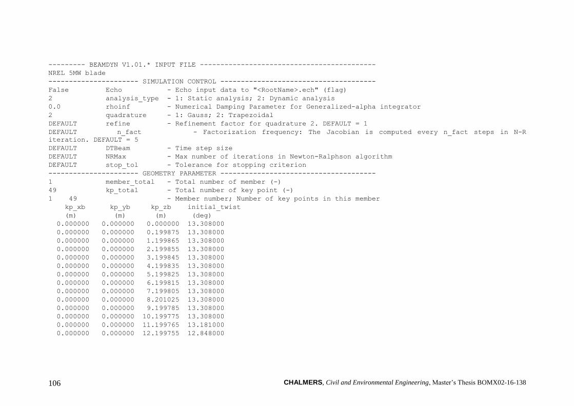
CHALMERS, Civil and Environmental Engineering, Master’s Thesis BOMX02-16-138 106
--------- BEAMDYN V1.01.* INPUT FILE -------------------------------------------
NREL 5MW blade
---------------------- SIMULATION CONTROL --------------------------------------
False Echo - Echo input data to "<RootName>.ech" (flag)
2 analysis_type - 1: Static analysis; 2: Dynamic analysis
0.0 rhoinf - Numerical Damping Parameter for Generalized-alpha integrator
2 quadrature - 1: Gauss; 2: Trapezoidal
DEFAULT refine - Refinement factor for quadrature 2. DEFAULT = 1
DEFAULT n_fact - Factorization frequency: The Jacobian is computed every n_fact steps in N-R
iteration. DEFAULT = 5
DEFAULT DTBeam - Time step size
DEFAULT NRMax - Max number of iterations in Newton-Ralphson algorithm
DEFAULT stop_tol - Tolerance for stopping criterion
---------------------- GEOMETRY PARAMETER --------------------------------------
1 member_total - Total number of member (-)
49 kp_total - Total number of key point (-)
1 49 - Member number; Number of key points in this member
kp_xb kp_yb kp_zb initial_twist
(m) (m) (m) (deg)
0.000000 0.000000 0.000000 13.308000
0.000000 0.000000 0.199875 13.308000
0.000000 0.000000 1.199865 13.308000
0.000000 0.000000 2.199855 13.308000
0.000000 0.000000 3.199845 13.308000
0.000000 0.000000 4.199835 13.308000
0.000000 0.000000 5.199825 13.308000
0.000000 0.000000 6.199815 13.308000
0.000000 0.000000 7.199805 13.308000
0.000000 0.000000 8.201025 13.308000
0.000000 0.000000 9.199785 13.308000
0.000000 0.000000 10.199775 13.308000
0.000000 0.000000 11.199765 13.181000
0.000000 0.000000 12.199755 12.848000

CHALMERS, Civil and Environmental Engineering, Master’s Thesis BOMX02-16-138 107
0.000000 0.000000 13.200975 12.192000
0.000000 0.000000 14.199735 11.561000
0.000000 0.000000 15.199725 11.072000
0.000000 0.000000 16.199715 10.792000
0.000000 0.000000 18.200925 10.232000
0.000000 0.000000 20.200290 9.672000
0.000000 0.000000 22.200270 9.110000
0.000000 0.000000 24.200250 8.534000
0.000000 0.000000 26.200230 7.932000
0.000000 0.000000 28.200825 7.321000
0.000000 0.000000 30.200190 6.711000
0.000000 0.000000 32.200170 6.122000
0.000000 0.000000 34.200150 5.546000
0.000000 0.000000 36.200130 4.971000
0.000000 0.000000 38.200725 4.401000
0.000000 0.000000 40.200090 3.834000
0.000000 0.000000 42.200070 3.332000
0.000000 0.000000 44.200050 2.890000
0.000000 0.000000 46.200030 2.503000
0.000000 0.000000 48.201240 2.116000
0.000000 0.000000 50.199990 1.730000
0.000000 0.000000 52.199970 1.342000
0.000000 0.000000 54.199950 0.954000
0.000000 0.000000 55.199940 0.760000
0.000000 0.000000 56.199930 0.574000
0.000000 0.000000 57.199920 0.404000
0.000000 0.000000 57.699915 0.319000
0.000000 0.000000 58.201140 0.253000
0.000000 0.000000 58.699905 0.216000
0.000000 0.000000 59.199900 0.178000
0.000000 0.000000 59.699895 0.140000
0.000000 0.000000 60.199890 0.101000
0.000000 0.000000 60.699885 0.062000

CHALMERS, Civil and Environmental Engineering, Master’s Thesis BOMX02-16-138 108
0.000000 0.000000 61.199880 0.023000
0.000000 0.000000 61.500000 0.000000
---------------------- MESH PARAMETER ------------------------------------------
5 order_elem - Order of interpolation (basis) function (-)
---------------------- MATERIAL PARAMETER --------------------------------------
"NRELOffshrBsline5MW_BeamDyn_Blade.dat" BldFile - Name of file containing properties for blade
---------------------- PITCH ACTUATOR PARAMETERS -------------------------------
False UsePitchAct - Whether a pitch actuator should be used (flag)
200 PitchJ - Pitch actuator inertia (kg-m^2) [used only when UsePitchAct is true]
2.0E+7 PitchK - Pitch actuator stiffness (kg-m^2/s^2) [used only when UsePitchAct is true]
5.0E+5 PitchC - Pitch actuator damping (kg-m^2/s) [used only when UsePitchAct is true]
---------------------- OUTPUTS -------------------------------------------------
True SumPrint - Print summary data to "<RootName>.sum" (flag)
"ES10.3E2" OutFmt - Format used for text tabular output, excluding the time channel. Resulting field
should be 10 characters. (quoted string)
0 NNodeOuts - Number of nodes to output to file [0 - 9] (-)
1,2,3,4,5,6 OutNd - Nodes whose values will be output (-)
OutList - The next line(s) contains a list of output parameters. See OutListParameters.xlsx
for a listing of available output channels, (-)
"RootFxr, RootFyr, RootFzr"
"RootMxr, RootMyr, RootMzr"
"TipTDxr, TipTDyr, TipTDzr"
"TipRDxr, TipRDyr, TipRDzr"
END of input file (the word "END" must appear in the first 3 columns of this last OutList line)
--------------------------------------------------------------------------------

CHALMERS, Civil and Environmental Engineering, Master’s Thesis BOMX02-16-138 109
------- InflowWind v3.01.* INPUT FILE -------------------------------------------------------------------------
Steady 57.09 m/s wind
---------------------------------------------------------------------------------------------------------------
False Echo - Echo input data to <RootName>.ech (flag)
1 WindType - switch for wind file type (1=steady; 2=uniform; 3=binary TurbSim FF; 4=binary Bladed-
style FF; 5=HAWC format; 6=User defined)
0 PropogationDir - Direction of wind propogation (meteoroligical rotation from aligned with X (positive
rotates towards -Y) -- degrees)
1 NWindVel - Number of points to output the wind velocity (0 to 9)
0 WindVxiList - List of coordinates in the inertial X direction (m)
0 WindVyiList - List of coordinates in the inertial Y direction (m)
90 WindVziList - List of coordinates in the inertial Z direction (m)
================== Parameters for Steady Wind Conditions [used only for WindType = 1] =========================
57.09 HWindSpeed - Horizontal windspeed
90 RefHt - Reference height for horizontal wind speed
0 PLexp - Power law exponent
================== Parameters for Uniform wind file [used only for WindType = 2] ============================
"Wind/08ms.wnd" Filename - Filename of time series data for uniform wind field.
90 RefHt - Reference height for horizontal wind speed
125.88 RefLength - Reference length for linear horizontal and vertical sheer
================== Parameters for Binary TurbSim Full-Field files [used only for WindType = 3] ==============
"Wind/08ms.wnd" Filename - Name of the Full field wind file to use (.bts)
================== Parameters for Binary Bladed-style Full-Field files [used only for WindType = 4] =========
"unused" FilenameRoot - Rootname of the full-field wind file to use (.wnd, .sum)
False TowerFile - Have tower file (.twr) [flag]
================== Parameters for HAWC-format binary files [Only used with WindType = 5] =====================
"wasp\Output\basic_5u.bin" FileName_u - name of the file containing the u-component fluctuating wind
"wasp\Output\basic_5v.bin" FileName_v - name of the file containing the v-component fluctuating wind
"wasp\Output\basic_5w.bin" FileName_w - name of the file containing the w-component fluctuating wind
64 nx - number of grids in the x direction (in the 3 files above)
32 ny - number of grids in the y direction (in the 3 files above)
32 nz - number of grids in the z direction (in the 3 files above)
16 dx - distance (in meters) between points in the x direction

CHALMERS, Civil and Environmental Engineering, Master’s Thesis BOMX02-16-138 110
3 dy - distance (in meters) between points in the y direction
3 dz - distance (in meters) between points in the z direction
90 RefHt - reference height; the height (in meters) of the vertical center of the grid
------------- Scaling parameters for turbulence ---------------------------------------------------------
1 ScaleMethod - Turbulence scaling method [0 = none, 1 = direct scaling, 2 = calculate scaling
factor based on a desired standard deviation]
1 SFx - Turbulence scaling factor for the x direction (-) [ScaleMethod=1]
1 SFy - Turbulence scaling factor for the y direction (-) [ScaleMethod=1]
1 SFz - Turbulence scaling factor for the z direction (-) [ScaleMethod=1]
12 SigmaFx - Turbulence standard deviation to calculate scaling from in x direction (m/s)
[ScaleMethod=2]
8 SigmaFy - Turbulence standard deviation to calculate scaling from in y direction (m/s)
[ScaleMethod=2]
2 SigmaFz - Turbulence standard deviation to calculate scaling from in z direction (m/s)
[ScaleMethod=2]
------------- Mean wind profile parameters (added to HAWC-format files) ---------------------------------
5 URef - Mean u-component wind speed at the reference height [m/s]
2 WindProfile - Wind profile type (0=constant;1=logarithmic,2=power law)
0 PLExp - Power law exponent [-] (used only when WindProfile=2)
0.03 Z0 - Surface roughness length [m] (used only when WindProfile=1)
====================== OUTPUT ==================================================================================
False SumPrint - Print summary data to <RootName>.IfW.sum (flag)
OutList - The next line(s) contains a list of output parameters. See OutListParameters.xlsx for
a listing of available output channels, (-)
"Wind1VelX" X-direction wind velocity at point WindList(1)
"Wind1VelY" Y-direction wind velocity at point WindList(1)
"Wind1VelZ" Z-direction wind velocity at point WindList(1)
END of input file (the word "END" must appear in the first 3 columns of this last OutList line)
---------------------------------------------------------------------------------------
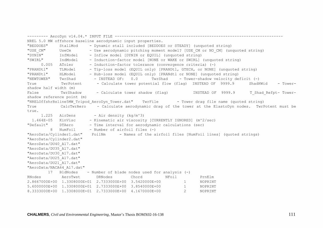
CHALMERS, Civil and Environmental Engineering, Master’s Thesis BOMX02-16-138 111
--------- AeroDyn v14.04.* INPUT FILE -------------------------------------------------------------------------
NREL 5.0 MW offshore baseline aerodynamic input properties.
"BEDDOES" StallMod - Dynamic stall included [BEDDOES or STEADY] (unquoted string)
"USE_CM" UseCm - Use aerodynamic pitching moment model? [USE_CM or NO_CM] (unquoted string)
"DYNIN" InfModel - Inflow model [DYNIN or EQUIL] (unquoted string)
"SWIRL" IndModel - Induction-factor model [NONE or WAKE or SWIRL] (unquoted string)
0.005 AToler - Induction-factor tolerance (convergence criteria) (-)
"PRANDtl" TLModel - Tip-loss model (EQUIL only) [PRANDtl, GTECH, or NONE] (unquoted string)
"PRANDtl" HLModel - Hub-loss model (EQUIL only) [PRANdtl or NONE] (unquoted string)
"NEWTOWER" TwrShad - INSTEAD OF: 0.0 TwrShad - Tower-shadow velocity deficit (-)
True TwrPotent - Calculate tower potential flow (flag) INSTEAD OF 9999.9 ShadHWid - Tower-
shadow half width (m)
False TwrShadow - Calculate tower shadow (flag) INSTEAD OF 9999.9 T_Shad_Refpt- Tower-
shadow reference point (m)
"NRELOffshrBsline5MW_Tripod_AeroDyn_Tower.dat" TwrFile - Tower drag file name (quoted string)
True CalcTwrAero - Calculate aerodynamic drag of the tower at the ElastoDyn nodes. TwrPotent must be
true.
1.225 AirDens - Air density (kg/m^3)
1.464E-05 KinVisc - Kinematic air viscosity [CURRENTLY IGNORED] (m^2/sec)
"Default" DTAero - Time interval for aerodynamic calculations (sec)
8 NumFoil - Number of airfoil files (-)
"AeroData/Cylinder1.dat" FoilNm - Names of the airfoil files [NumFoil lines] (quoted strings)
"AeroData/Cylinder2.dat"
"AeroData/DU40_A17.dat"
"AeroData/DU35_A17.dat"
"AeroData/DU30_A17.dat"
"AeroData/DU25_A17.dat"
"AeroData/DU21_A17.dat"
"AeroData/NACA64_A17.dat"
17 BldNodes - Number of blade nodes used for analysis (-)
RNodes AeroTwst DRNodes Chord NFoil PrnElm
2.8667000E+00 1.3308000E+01 2.7333000E+00 3.5420000E+00 1 NOPRINT
5.6000000E+00 1.3308000E+01 2.7333000E+00 3.8540000E+00 1 NOPRINT
8.3333000E+00 1.3308000E+01 2.7333000E+00 4.1670000E+00 2 NOPRINT

CHALMERS, Civil and Environmental Engineering, Master’s Thesis BOMX02-16-138 112
1.1750000E+01 1.3308000E+01 4.1000000E+00 4.5570000E+00 3 NOPRINT
1.5850000E+01 1.1480000E+01 4.1000000E+00 4.6520000E+00 4 NOPRINT
1.9950000E+01 1.0162000E+01 4.1000000E+00 4.4580000E+00 4 NOPRINT
2.4050000E+01 9.0110000E+00 4.1000000E+00 4.2490000E+00 5 NOPRINT
2.8150000E+01 7.7950000E+00 4.1000000E+00 4.0070000E+00 6 NOPRINT
3.2250000E+01 6.5440000E+00 4.1000000E+00 3.7480000E+00 6 NOPRINT
3.6350000E+01 5.3610000E+00 4.1000000E+00 3.5020000E+00 7 NOPRINT
4.0450000E+01 4.1880000E+00 4.1000000E+00 3.2560000E+00 7 NOPRINT
4.4550000E+01 3.1250000E+00 4.1000000E+00 3.0100000E+00 8 NOPRINT
4.8650000E+01 2.3190000E+00 4.1000000E+00 2.7640000E+00 8 NOPRINT
5.2750000E+01 1.5260000E+00 4.1000000E+00 2.5180000E+00 8 NOPRINT
5.6166700E+01 8.6300000E-01 2.7333000E+00 2.3130000E+00 8 NOPRINT
5.8900000E+01 3.7000000E-01 2.7333000E+00 2.0860000E+00 8 NOPRINT
6.1633300E+01 1.0600000E-01 2.7333000E+00 1.4190000E+00 8 NOPRINT

CHALMERS, Civil and Environmental Engineering, Master’s Thesis BOMX02-16-138 113
------- SERVODYN v1.03.* INPUT FILE --------------------------------------------
Master’s Thesis: Assessment of Simulation Codes for Offshore Wind Turbine Foundations – DNV load case 6.1c
---------------------- SIMULATION CONTROL --------------------------------------
False Echo - Echo input data to <RootName>.ech (flag)
"DEFAULT" DT - Communication interval for controllers (s) (or "default")
---------------------- PITCH CONTROL -------------------------------------------
5 PCMode - Pitch control mode 0: none, 3: user-defined from routine PitchCntrl, 4: user-defined
from Simulink/Labview, 5: user-defined from Bladed-style DLL (switch)
0 TPCOn - Time to enable active pitch control (s) [unused when PCMode=0]
0 TPitManS(1) - Time to start override pitch maneuver for blade 1 and end standard pitch control (s)
0 TPitManS(2) - Time to start override pitch maneuver for blade 2 and end standard pitch control (s)
0 TPitManS(3) - Time to start override pitch maneuver for blade 3 and end standard pitch control (s)
[unused for 2 blades]
8 PitManRat(1) - Pitch rate at which override pitch maneuver heads toward final pitch angle for blade 1
(deg/s)
8 PitManRat(2) - Pitch rate at which override pitch maneuver heads toward final pitch angle for blade 2
(deg/s)
8 PitManRat(3) - Pitch rate at which override pitch maneuver heads toward final pitch angle for blade 3
(deg/s) [unused for 2 blades]
90 BlPitchF(1) - Blade 1 final pitch for pitch maneuvers (degrees)
90 BlPitchF(2) - Blade 2 final pitch for pitch maneuvers (degrees)
90 BlPitchF(3) - Blade 3 final pitch for pitch maneuvers (degrees) [unused for 2 blades]
---------------------- GENERATOR AND TORQUE CONTROL ----------------------------
5 VSContrl - Variable-speed control mode 0: none, 1: simple VS, 3: user-defined from routine
UserVSCont, 4: user-defined from Simulink/Labview, 5: user-defined from Bladed-style DLL (switch)
2 GenModel - Generator model 1: simple, 2: Thevenin, 3: user-defined from routine UserGen (switch)
[used only when VSContrl=0]
94.4 GenEff - Generator efficiency [ignored by the Thevenin and user-defined generator models] (%)
True GenTiStr - Method to start the generator T: timed using TimGenOn, F: generator speed using
SpdGenOn (flag)
True GenTiStp - Method to stop the generator T: timed using TimGenOf, F: when generator power = 0
(flag)
9999.9 SpdGenOn - Generator speed to turn on the generator for a startup (HSS speed) (rpm) [used only
when GenTiStr=False]

CHALMERS, Civil and Environmental Engineering, Master’s Thesis BOMX02-16-138 114
0 TimGenOn - Time to turn on the generator for a startup (s) [used only when GenTiStr=True]
9999.9 TimGenOf - Time to turn off the generator (s) [used only when GenTiStp=True]
---------------------- SIMPLE VARIABLE-SPEED TORQUE CONTROL --------------------
9999.9 VS_RtGnSp - Rated generator speed for simple variable-speed generator control (HSS side) (rpm)
[used only when VSContrl=1]
9999.9 VS_RtTq - Rated generator torque/constant generator torque in Region 3 for simple variable-speed
generator control (HSS side) (N-m) [used only when VSContrl=1]
9999.9 VS_Rgn2K - Generator torque constant in Region 2 for simple variable-speed generator control (HSS
side) (N-m/rpm^2) [used only when VSContrl=1]
9999.9 VS_SlPc - Rated generator slip percentage in Region 2 1/2 for simple variable-speed generator
control (%) [used only when VSContrl=1]
---------------------- SIMPLE INDUCTION GENERATOR ------------------------------
9999.9 SIG_SlPc - Rated generator slip percentage (%) [used only when VSContrl=0 and GenModel=1]
9999.9 SIG_SySp - Synchronous (zero-torque) generator speed (rpm) [used only when VSContrl=0 and
GenModel=1]
9999.9 SIG_RtTq - Rated torque (N-m) [used only when VSContrl=0 and GenModel=1]
9999.9 SIG_PORt - Pull-out ratio (Tpullout/Trated) (-) [used only when VSContrl=0 and GenModel=1]
---------------------- THEVENIN-EQUIVALENT INDUCTION GENERATOR -----------------
9999.9 TEC_Freq - Line frequency [50 or 60] (Hz) [used only when VSContrl=0 and GenModel=2]
9998 TEC_NPol - Number of poles [even integer > 0] (-) [used only when VSContrl=0 and GenModel=2]
9999.9 TEC_SRes - Stator resistance (ohms) [used only when VSContrl=0 and GenModel=2]
9999.9 TEC_RRes - Rotor resistance (ohms) [used only when VSContrl=0 and GenModel=2]
9999.9 TEC_VLL - Line-to-line RMS voltage (volts) [used only when VSContrl=0 and GenModel=2]
9999.9 TEC_SLR - Stator leakage reactance (ohms) [used only when VSContrl=0 and GenModel=2]
9999.9 TEC_RLR - Rotor leakage reactance (ohms) [used only when VSContrl=0 and GenModel=2]
9999.9 TEC_MR - Magnetizing reactance (ohms) [used only when VSContrl=0 and GenModel=2]
---------------------- HIGH-SPEED SHAFT BRAKE ----------------------------------
1 HSSBrMode - HSS brake model 0: none, 1: simple, 3: user-defined from routine UserHSSBr, 4: user-
defined from Simulink/Labview, 5: user-defined from Bladed-style DLL (switch)
0 THSSBrDp - Time to initiate deployment of the HSS brake (s)
0.2 HSSBrDT - Time for HSS-brake to reach full deployment once initiated (sec) [used only when
HSSBrMode=1]
281160.2 HSSBrTqF - Fully deployed HSS-brake torque (N-m)
---------------------- NACELLE-YAW CONTROL -------------------------------------

CHALMERS, Civil and Environmental Engineering, Master’s Thesis BOMX02-16-138 115
0 YCMode - Yaw control mode 0: none, 3: user-defined from routine UserYawCont, 4: user-defined
from Simulink/Labview, 5: user-defined from Bladed-style DLL (switch)
9999.9 TYCOn - Time to enable active yaw control (s) [unused when YCMode=0]
0 YawNeut - Neutral yaw position--yaw spring force is zero at this yaw (degrees)
9.02832E+09 YawSpr - Nacelle-yaw spring constant (N-m/rad)
1.916E+07 YawDamp - Nacelle-yaw damping constant (N-m/(rad/s))
9999.9 TYawManS - Time to start override yaw maneuver and end standard yaw control (s)
0.3 YawManRat - Yaw maneuver rate (in absolute value) (deg/s)
0 NacYawF - Final yaw angle for override yaw maneuvers (degrees)
---------------------- TUNED MASS DAMPER ---------------------------------------
False CompNTMD - Compute nacelle tuned mass damper true/false (flag)
"unused" NTMDfile - Name of the file for nacelle tuned mass damper (quoted string) [unused when CompNTMD is
false]
---------------------- BLADED INTERFACE ----------------------------------------
"ServoData\DISCON_win32.dll" DLL_FileName - Name/location of the dynamic library .dll [Windows] or .so [Linux]
in the Bladed-DLL format (-) [used only with Bladed Interface]
"DISCON.IN" DLL_InFile - Name of input file sent to the DLL [used only with Bladed Interface] (-)
"default" DLL_DT - Communication interval for dynamic library [used only with Bladed Interface] (s) (or
"default")
false DLL_Ramp - Whether a linear ramp should be used between DLL_DT time steps [introduces time shift
when true] (flag)
9999.9 BPCutoff - Cuttoff frequency for low-pass filter on blade pitch from DLL (Hz)
0 NacYaw_North - Reference yaw angle of the nacelle when the upwind end points due North (deg) [used
only with Bladed Interface]
0 Ptch_Cntrl - Record 28: Use individual pitch control 0: collective pitch; 1: individual pitch
control (switch) [used only with Bladed Interface]
0 Ptch_SetPnt - Record 5: Below-rated pitch angle set-point (deg) [used only with Bladed Interface]
0 Ptch_Min - Record 6: Minimum pitch angle (deg) [used only with Bladed Interface]
0 Ptch_Max - Record 7: Maximum pitch angle (deg) [used only with Bladed Interface]
0 PtchRate_Min - Record 8: Minimum pitch rate (most negative value allowed) (deg/s) [used only with
Bladed Interface]
0 PtchRate_Max - Record 9: Maximum pitch rate (deg/s) [used only with Bladed Interface]
0 Gain_OM - Record 16: Optimal mode gain (Nm/(rad/s)^2) [used only with Bladed Interface]
0 GenSpd_MinOM - Record 17: Minimum generator speed (rpm) [used only with Bladed Interface]

CHALMERS, Civil and Environmental Engineering, Master’s Thesis BOMX02-16-138 116
0 GenSpd_MaxOM - Record 18: Optimal mode maximum speed (rpm) [used only with Bladed Interface]
0 GenSpd_Dem - Record 19: Demanded generator speed above rated (rpm) [used only with Bladed Interface]
0 GenTrq_Dem - Record 22: Demanded generator torque above rated (Nm) [used only with Bladed Interface]
0 GenPwr_Dem - Record 13: Demanded power (W) [used only with Bladed Interface]
---------------------- BLADED INTERFACE TORQUE-SPEED LOOK-UP TABLE -------------
0 DLL_NumTrq - Record 26: No. of points in torque-speed look-up table 0 = none and use the optimal
mode parameters; nonzero = ignore the optimal mode PARAMETERs by setting Record 16 to 0.0 (-) [used only with
Bladed Interface]
GenSpd_TLU GenTrq_TLU
(rpm) (Nm)
---------------------- OUTPUT --------------------------------------------------
True SumPrint - Print summary data to <RootName>.sum (flag) (currently unused)
2 OutFile - Switch to determine where output will be placed: 1: in module output file only; 2: in
glue code output file only; 3: both (currently unused)
True TabDelim - Use tab delimiters in text tabular output file? (flag) (currently unused)
"ES10.3E2" OutFmt - Format used for text tabular output (except time). Resulting field should be 10
characters. (quoted string) (currently unused)
30 TStart - Time to begin tabular output (s) (currently unused)
OutList - The next line(s) contains a list of output parameters. See OutListParameters.xlsx for
a listing of available output channels, (-)
"GenPwr" - Electrical generator power and torque
"GenTq" - Electrical generator power and torque
END of input file (the word "END" must appear in the first 3 columns of this last OutList line)
---------------------------------------------------------------------------------------
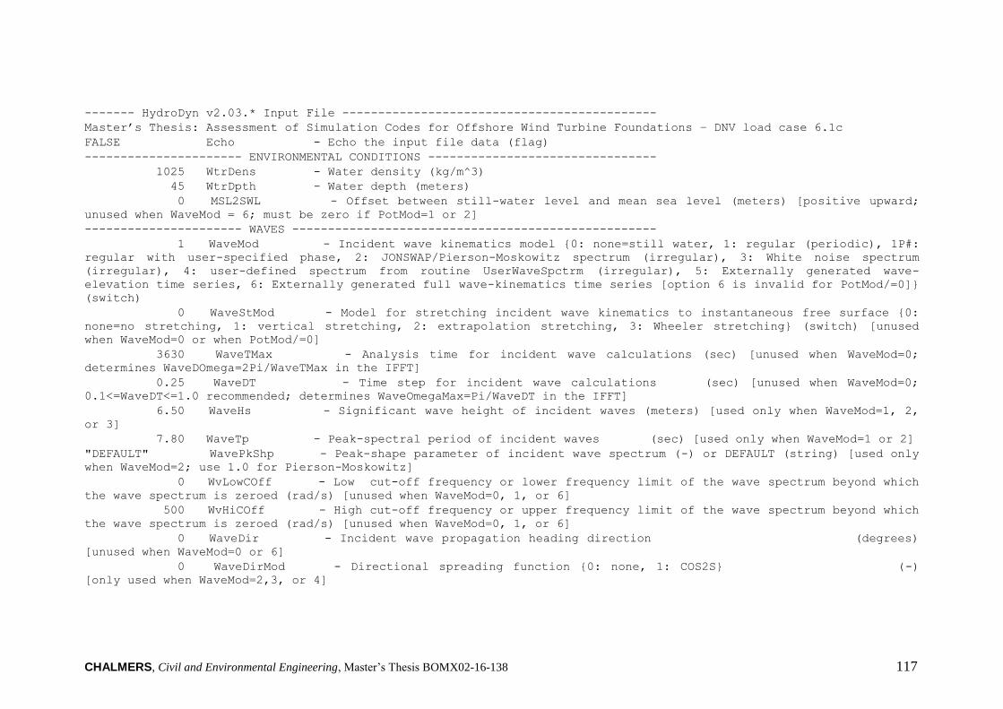
CHALMERS, Civil and Environmental Engineering, Master’s Thesis BOMX02-16-138 117
------- HydroDyn v2.03.* Input File --------------------------------------------
Master’s Thesis: Assessment of Simulation Codes for Offshore Wind Turbine Foundations – DNV load case 6.1c
FALSE Echo - Echo the input file data (flag)
---------------------- ENVIRONMENTAL CONDITIONS --------------------------------
1025 WtrDens - Water density (kg/m^3)
45 WtrDpth - Water depth (meters)
0 MSL2SWL - Offset between still-water level and mean sea level (meters) [positive upward;
unused when WaveMod = 6; must be zero if PotMod=1 or 2]
---------------------- WAVES ---------------------------------------------------
1 WaveMod - Incident wave kinematics model 0: none=still water, 1: regular (periodic), 1P#:
regular with user-specified phase, 2: JONSWAP/Pierson-Moskowitz spectrum (irregular), 3: White noise spectrum
(irregular), 4: user-defined spectrum from routine UserWaveSpctrm (irregular), 5: Externally generated wave-
elevation time series, 6: Externally generated full wave-kinematics time series [option 6 is invalid for PotMod/=0]
(switch)
0 WaveStMod - Model for stretching incident wave kinematics to instantaneous free surface 0:
none=no stretching, 1: vertical stretching, 2: extrapolation stretching, 3: Wheeler stretching (switch) [unused
when WaveMod=0 or when PotMod/=0]
3630 WaveTMax - Analysis time for incident wave calculations (sec) [unused when WaveMod=0;
determines WaveDOmega=2Pi/WaveTMax in the IFFT]
0.25 WaveDT - Time step for incident wave calculations (sec) [unused when WaveMod=0;
0.1<=WaveDT<=1.0 recommended; determines WaveOmegaMax=Pi/WaveDT in the IFFT]
6.50 WaveHs - Significant wave height of incident waves (meters) [used only when WaveMod=1, 2,
or 3]
7.80 WaveTp - Peak-spectral period of incident waves (sec) [used only when WaveMod=1 or 2]
"DEFAULT" WavePkShp - Peak-shape parameter of incident wave spectrum (-) or DEFAULT (string) [used only
when WaveMod=2; use 1.0 for Pierson-Moskowitz]
0 WvLowCOff - Low cut-off frequency or lower frequency limit of the wave spectrum beyond which
the wave spectrum is zeroed (rad/s) [unused when WaveMod=0, 1, or 6]
500 WvHiCOff - High cut-off frequency or upper frequency limit of the wave spectrum beyond which
the wave spectrum is zeroed (rad/s) [unused when WaveMod=0, 1, or 6]
0 WaveDir - Incident wave propagation heading direction (degrees)
[unused when WaveMod=0 or 6]
0 WaveDirMod - Directional spreading function 0: none, 1: COS2S (-)
[only used when WaveMod=2,3, or 4]

CHALMERS, Civil and Environmental Engineering, Master’s Thesis BOMX02-16-138 118
1 WaveDirSpread - Wave direction spreading coefficient ( > 0 ) (-)
[only used when WaveMod=2,3, or 4 and WaveDirMod=1]
1 WaveNDir - Number of wave directions (-)
[only used when WaveMod=2,3, or 4 and WaveDirMod=1; odd number only]
0 WaveDirRange - Range of wave directions (full range: WaveDir +/- 1/2*WaveDirRange) (degrees)
[only used when WaveMod=2,3,or 4 and WaveDirMod=1]
123456789 WaveSeed(1) - First random seed of incident waves [-2147483648 to 2147483647] (-)
[unused when WaveMod=0, 5, or 6]
1011121314 WaveSeed(2) - Second random seed of incident waves [-2147483648 to 2147483647] (-)
[unused when WaveMod=0, 5, or 6]
False WaveNDAmp - Flag for normally distributed amplitudes (flag)
[only used when WaveMod=2, 3, or 4]
"" WvKinFile - Root name of externally generated wave data file(s) (quoted string)
[used only when WaveMod=5 or 6]
1 NWaveElev - Number of points where the incident wave elevations can be computed (-)
[maximum of 9 output locations]
0 WaveElevxi - List of xi-coordinates for points where the incident wave elevations can be output
(meters) [NWaveElev points, separated by commas or white space; usused if NWaveElev = 0]
0 WaveElevyi - List of yi-coordinates for points where the incident wave elevations can be output
(meters) [NWaveElev points, separated by commas or white space; usused if NWaveElev = 0]
---------------------- 2ND-ORDER WAVES ----------------------------------------- [unused with WaveMod=0 or 6]
False WvDiffQTF - Full difference-frequency 2nd-order wave kinematics (flag)
False WvSumQTF - Full summation-frequency 2nd-order wave kinematics (flag)
0 WvLowCOffD - Low frequency cutoff used in the difference-frequencies (rad/s) [Only used with a
difference-frequency method]
3.5 WvHiCOffD - High frequency cutoff used in the difference-frequencies (rad/s) [Only used with a
difference-frequency method]
0.1 WvLowCOffS - Low frequency cutoff used in the summation-frequencies (rad/s) [Only used with a
summation-frequency method]
3.5 WvHiCOffS - High frequency cutoff used in the summation-frequencies (rad/s) [Only used with a
summation-frequency method]
---------------------- CURRENT ------------------------------------------------- [unused with WaveMod=6]
1 CurrMod - Current profile model 0: none=no current, 1: standard, 2: user-defined from
routine UserCurrent (switch)

CHALMERS, Civil and Environmental Engineering, Master’s Thesis BOMX02-16-138 119
0 CurrSSV0 - Sub-surface current velocity at still water level (m/s) [used only when
CurrMod=1]
0 CurrSSDir - Sub-surface current heading direction (degrees) or DEFAULT (string) [used only
when CurrMod=1]
20 CurrNSRef - Near-surface current reference depth (meters) [used only when
CurrMod=1]
0 CurrNSV0 - Near-surface current velocity at still water level (m/s) [used only when
CurrMod=1]
0 CurrNSDir - Near-surface current heading direction (degrees) [used only when
CurrMod=1]
0.89 CurrDIV - Depth-independent current velocity (m/s) [used only when
CurrMod=1]
0 CurrDIDir - Depth-independent current heading direction (degrees) [used only when
CurrMod=1]
---------------------- FLOATING PLATFORM --------------------------------------- [unused with WaveMod=6]
0 PotMod - Potential-flow model 0: none=no potential flow, 1: frequency-to-time-domain
transforms based on WAMIT output, 2: fluid-impulse theory (FIT) (switch)
"unused" PotFile - Root name of potential-flow model data; WAMIT output files containing the linear,
nondimensionalized, hydrostatic restoring matrix (.hst), frequency-dependent hydrodynamic added mass matrix and
damping matrix (.1), and frequency- and direction-dependent wave excitation force vector per unit wave amplitude
(.3) (quoted string) [MAKE SURE THE FREQUENCIES INHERENT IN THESE WAMIT FILES SPAN THE PHYSICALLY-SIGNIFICANT RANGE
OF FREQUENCIES FOR THE GIVEN PLATFORM; THEY MUST CONTAIN THE ZERO- AND INFINITE-FREQUENCY LIMITS!]
1 WAMITULEN - Characteristic body length scale used to redimensionalize WAMIT output (meters)
[only used when PotMod=1]
0 PtfmVol0 - Displaced volume of water when the platform is in its undisplaced position (m^3)
[only used when PotMod=1; USE THE SAME VALUE COMPUTED BY WAMIT AS OUTPUT IN THE .OUT FILE!]
0 PtfmCOBxt - The xt offset of the center of buoyancy (COB) from the platform reference point
(meters) [only used when PotMod=1]
0 PtfmCOByt - The yt offset of the center of buoyancy (COB) from the platform reference point
(meters) [only used when PotMod=1]
1 RdtnMod - Radiation memory-effect model 0: no memory-effect calculation, 1: convolution, 2:
state-space (switch) [only used when PotMod=1; STATE-SPACE REQUIRES *.ss INPUT FILE]
60 RdtnTMax - Analysis time for wave radiation kernel calculations (sec) [only used when
PotMod=1; determines RdtnDOmega=Pi/RdtnTMax in the cosine transform; MAKE SURE THIS IS LONG ENOUGH FOR THE RADIATION
IMPULSE RESPONSE FUNCTIONS TO DECAY TO NEAR-ZERO FOR THE GIVEN PLATFORM!]

CHALMERS, Civil and Environmental Engineering, Master’s Thesis BOMX02-16-138 120
0.025 RdtnDT - Time step for wave radiation kernel calculations (sec) [only used when PotMod=1;
DT<=RdtnDT<=0.1 recommended; determines RdtnOmegaMax=Pi/RdtnDT in the cosine transform]
---------------------- 2ND-ORDER FLOATING PLATFORM FORCES ---------------------- [unused with WaveMod=0 or 6, or
PotMod=0 or 2]
0 MnDrift - Mean-drift 2nd-order forces computed 0:
None; [7, 8, 9, 10, 11, or 12]: WAMIT file to use [Only one of MnDrift, NewmanApp, or DiffQTF can be non-zero]
0 NewmanApp - Mean- and slow-drift 2nd-order forces computed with Newman's approximation 0:
None; [7, 8, 9, 10, 11, or 12]: WAMIT file to use [Only one of MnDrift, NewmanApp, or DiffQTF can be non-zero. Used
only when WaveDirMod=0]
0 DiffQTF - Full difference-frequency 2nd-order forces computed with full QTF 0:
None; [10, 11, or 12]: WAMIT file to use [Only one of MnDrift, NewmanApp, or DiffQTF can be non-zero]
0 SumQTF - Full summation -frequency 2nd-order forces computed with full QTF 0:
None; [10, 11, or 12]: WAMIT file to use
---------------------- FLOATING PLATFORM FORCE FLAGS -------------------------- [unused with WaveMod=6]
True PtfmSgF - Platform horizontal surge translation force (flag) or DEFAULT
True PtfmSwF - Platform horizontal sway translation force (flag) or DEFAULT
True PtfmHvF - Platform vertical heave translation force (flag) or DEFAULT
True PtfmRF - Platform roll tilt rotation force (flag) or DEFAULT
True PtfmPF - Platform pitch tilt rotation force (flag) or DEFAULT
True PtfmYF - Platform yaw rotation force (flag) or DEFAULT
---------------------- PLATFORM ADDITIONAL STIFFNESS AND DAMPING --------------
0 0 0 0 0 0 AddF0 - Additional preload
(N, N-m)
0 0 0 0 0 0 AddCLin - Additional linear
stiffness (N/m, N/rad, N-m/m, N-m/rad)
0 0 0 0 0 0
0 0 0 0 0 0
0 0 0 0 0 0
0 0 0 0 0 0
0 0 0 0 0 0
0 0 0 0 0 0 AddBLin - Additional linear
damping(N/(m/s), N/(rad/s), N-m/(m/s), N-m/(rad/s))
0 0 0 0 0 0
0 0 882607 0 0 0

CHALMERS, Civil and Environmental Engineering, Master’s Thesis BOMX02-16-138 121
0 0 0 0 0 0
0 0 0 0 0 0
0 0 0 0 0 0
0 0 0 0 0 0 AddBQuad - Additional
quadratic drag(N/(m/s)^2, N/(rad/s)^2, N-m(m/s)^2, N-m/(rad/s)^2)
0 0 0 0 0 0
0 0 0 0 0 0
0 0 0 0 0 0
0 0 0 0 0 0
0 0 0 0 0 0
---------------------- AXIAL COEFFICIENTS --------------------------------------
1 NAxCoef - Number of axial coefficients (-)
AxCoefID AxCd AxCa AxCp
(-) (-) (-) (-)
1 1.00 1.00 1.00
---------------------- MEMBER JOINTS -------------------------------------------
67 NJoints - Number of joints (-) [must be exactly 0 or at least 2]
JointID Jointxi Jointyi Jointzi JointAxID JointOvrlp [JointOvrlp= 0: do nothing at joint. 1:
eliminate overlaps by calculating super member]
(-) (m) (m) (m) (-) (switch)
1 0 25.7637000000000 -35 1 0
2 22.3120000000000 -12.8818000000000 -35 1 0
3 -22.3120000000000 -12.8818000000000 -35 1 0
4 0 0 -35 1 0
5 0 25.7637000000000 -25 1 0
6 22.3120000000000 -12.8818000000000 -25 1 0
7 -22.3120000000000 -12.8818000000000 -25 1 0
8 0 25.7637000000000 -45.01 1 0
9 22.3120000000000 -12.8818000000000 -45.01 1 0
10 -22.3120000000000 -12.8818000000000 -45.01 1 0
11 0 0 0 1 0
12 0 0 10 1 0
13 0 0 -37 1 0

CHALMERS, Civil and Environmental Engineering, Master’s Thesis BOMX02-16-138 122
14 0 19.3227750000000 -35 1 0
15 0 12.8818500000000 -35 1 0
16 0 6.44092500000000 -35 1 0
17 16.7340000000000 -9.66135000000000 -35 1 0
18 11.1560000000000 -6.44090000000000 -35 1 0
19 5.57800000000000 -3.22045000000000 -35 1 0
20 -16.7340000000000 -9.66135000000000 -35 1 0
21 -11.1560000000000 -6.44090000000000 -35 1 0
22 -5.57800000000000 -3.22045000000000 -35 1 0
23 0 25.7637000000000 -32.5000000000000 1 0
24 0 25.7637000000000 -30 1 0
25 0 25.7637000000000 -27.5000000000000 1 0
26 22.3120000000000 -12.8818000000000 -32.5000000000000 1 0
27 22.3120000000000 -12.8818000000000 -30 1 0
28 22.3120000000000 -12.8818000000000 -27.5000000000000 1 0
29 -22.3120000000000 -12.8818000000000 -32.5000000000000 1 0
30 -22.3120000000000 -12.8818000000000 -30 1 0
31 -22.3120000000000 -12.8818000000000 -27.5000000000000 1 0
32 0 25.7637000000000 -42.5000000000000 1 0
33 0 25.7637000000000 -40 1 0
34 0 25.7637000000000 -37.5000000000000 1 0
35 22.3120000000000 -12.8818000000000 -42.5000000000000 1 0
36 22.3120000000000 -12.8818000000000 -40 1 0
37 22.3120000000000 -12.8818000000000 -37.5000000000000 1 0
38 -22.3120000000000 -12.8818000000000 -42.5000000000000 1 0
39 -22.3120000000000 -12.8818000000000 -40 1 0
40 -22.3120000000000 -12.8818000000000 -37.5000000000000 1 0
41 5.57800000000000 16.1023250000000 -35 1 0
42 11.1560000000000 6.44095000000000 -35 1 0
43 16.7340000000000 -3.22042500000000 -35 1 0
44 11.1560000000000 -12.8818000000000 -35 1 0
45 0 -12.8818000000000 -35 1 0
46 -11.1560000000000 -12.8818000000000 -35 1 0

CHALMERS, Civil and Environmental Engineering, Master’s Thesis BOMX02-16-138 123
47 -16.7340000000000 -3.22042500000000 -35 1 0
48 -11.1560000000000 6.44095000000000 -35 1 0
49 -5.57800000000000 16.1023250000000 -35 1 0
50 0 0 -36.5000000000000 1 0
51 0 0 -36 1 0
52 0 0 -35.5000000000000 1 0
53 0 0 -26.2500000000000 1 0
54 0 0 -17.5000000000000 1 0
55 0 0 -8.75000000000000 1 0
56 0 19.3227750000000 -26.2500000000000 1 0
57 0 12.8818500000000 -17.5000000000000 1 0
58 0 6.44092500000000 -8.75000000000000 1 0
59 16.7340000000000 -9.66135000000000 -26.2500000000000 1 0
60 11.1560000000000 -6.44090000000000 -17.5000000000000 1 0
61 5.57800000000000 -3.22045000000000 -8.75000000000000 1 0
62 -16.7340000000000 -9.66135000000000 -26.2500000000000 1 0
63 -11.1560000000000 -6.44090000000000 -17.5000000000000 1 0
64 -5.57800000000000 -3.22045000000000 -8.75000000000000 1 0
65 0 0 2.50000000000000 1 0
66 0 0 5 1 0
67 0 0 7.50000000000000 1 0
---------------------- MEMBER CROSS-SECTION PROPERTIES -------------------------
72 NPropSets - Number of member property sets (-)
PropSetID PropD PropThck
(-) (m) (m)
1 0.800000000000000 0.0280000000000000
2 0.800000000000000 0.0280000000000000
3 0.800000000000000 0.0280000000000000
4 0.800000000000000 0.0280000000000000
5 0.800000000000000 0.0280000000000000
6 0.800000000000000 0.0280000000000000
7 0.800000000000000 0.0280000000000000
8 0.800000000000000 0.0280000000000000

CHALMERS, Civil and Environmental Engineering, Master’s Thesis BOMX02-16-138 124
9 0.800000000000000 0.0280000000000000
10 0.800000000000000 0.0280000000000000
11 0.800000000000000 0.0280000000000000
12 0.800000000000000 0.0280000000000000
13 4 0.0400000000000000
14 4 0.0400000000000000
15 4 0.0400000000000000
16 4 0.0400000000000000
17 4 0.0400000000000000
18 4 0.0400000000000000
19 4 0.0400000000000000
20 4 0.0400000000000000
21 4 0.0400000000000000
22 4 0.0400000000000000
23 4 0.0400000000000000
24 4 0.0400000000000000
25 4 0.0400000000000000
26 4 0.0400000000000000
27 4 0.0400000000000000
28 4 0.0400000000000000
29 4 0.0400000000000000
30 4 0.0400000000000000
31 4 0.0400000000000000
32 4 0.0400000000000000
33 4 0.0400000000000000
34 4 0.0400000000000000
35 4 0.0400000000000000
36 4 0.0400000000000000
37 0.800000000000000 0.0160000000000000
38 0.800000000000000 0.0160000000000000
39 0.800000000000000 0.0160000000000000
40 0.800000000000000 0.0160000000000000
41 0.800000000000000 0.0160000000000000

CHALMERS, Civil and Environmental Engineering, Master’s Thesis BOMX02-16-138 125
42 0.800000000000000 0.0160000000000000
43 0.800000000000000 0.0160000000000000
44 0.800000000000000 0.0160000000000000
45 0.800000000000000 0.0160000000000000
46 0.800000000000000 0.0160000000000000
47 0.800000000000000 0.0160000000000000
48 0.800000000000000 0.0160000000000000
49 4 0.0280000000000000
50 4.02702500000000 0.0285500000000000
51 4.05405000000000 0.0291000000000000
52 4.08107500000000 0.0296500000000000
53 4.10810000000000 0.0302000000000000
54 4.58107500000000 0.0396500000000000
55 5.05405000000000 0.0491000000000000
56 5.52702500000000 0.0585500000000000
57 1.20000000000000 0.0320000000000000
58 1.20000000000000 0.0320000000000000
59 1.20000000000000 0.0320000000000000
60 1.20000000000000 0.0320000000000000
61 1.20000000000000 0.0320000000000000
62 1.20000000000000 0.0320000000000000
63 1.20000000000000 0.0320000000000000
64 1.20000000000000 0.0320000000000000
65 1.20000000000000 0.0320000000000000
66 1.20000000000000 0.0320000000000000
67 1.20000000000000 0.0320000000000000
68 1.20000000000000 0.0320000000000000
69 6 0.0400000000000000
70 6 0.0400000000000000
71 6 0.0400000000000000
72 6 0.0400000000000000
---------------------- SIMPLE HYDRODYNAMIC COEFFICIENTS (model 1) --------------

CHALMERS, Civil and Environmental Engineering, Master’s Thesis BOMX02-16-138 126
SimplCd SimplCdMG SimplCa SimplCaMG SimplCp SimplCpMG SimplAxCa SimplAxCaMG SimplAxCp
SimplAxCpMG
(-) (-) (-) (-) (-) (-) (-) (-) (-)
(-)
1.00 0.00 1.00 0.00 1.00 0.00 1.00 0.00 1.00
0.00
---------------------- DEPTH-BASED HYDRODYNAMIC COEFFICIENTS (model 2) ---------
0 NCoefDpth - Number of depth-dependent coefficients (-)
Dpth DpthCd DpthCdMG DpthCa DpthCaMG DpthCp DpthCpMG DpthAxCa DpthAxCaMG DpthAxCp
DpthAxCpMG
(m) (-) (-) (-) (-) (-) (-) (-) (-) (-)
(-)
---------------------- MEMBER-BASED HYDRODYNAMIC COEFFICIENTS (model 3) --------
0 NCoefMembers - Number of member-based coefficients (-)
MemberID MemberCd1 MemberCd2 MemberCdMG1 MemberCdMG2 MemberCa1 MemberCa2 MemberCaMG1
MemberCaMG2 MemberCp1 MemberCp2 MemberCpMG1 MemberCpMG2 MemberAxCa1 MemberAxCa2 MemberAxCaMG1
MemberAxCaMG2 MemberAxCp1 MemberAxCp2 MemberAxCpMG1 MemberAxCpMG2
(-) (-) (-) (-) (-) (-) (-) (-) (-)
(-) (-) (-) (-) (-) (-) (-) (-) (-)
(-) (-) (-)
-------------------- MEMBERS -------------------------------------------------
72 NMembers - Number of members (-)
MemberID MJointID1 MJointID2 MPropSetID1 MPropSetID2 MDivSize MCoefMod PropPot [MCoefMod=1: use simple
coeff table. 2: use depth-based coeff table. 3: use member-based coeff table] [ PropPot/=0 if member is modeled with
potential-flow theory]
(-) (-) (-) (-) (-) (m) (switch) (flag)
1 1 14 1 1 1 1 FALSE
2 14 15 2 2 1 1 FALSE
3 15 16 3 3 1 1 FALSE
4 16 4 4 4 1 1 FALSE
5 2 17 5 5 1 1 FALSE
6 17 18 6 6 1 1 FALSE
7 18 19 7 7 1 1 FALSE
8 19 4 8 8 1 1 FALSE
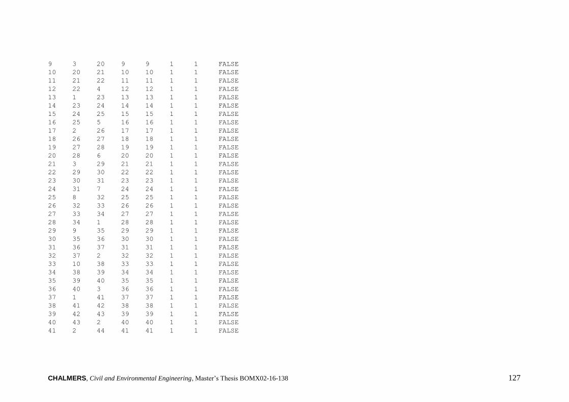
CHALMERS, Civil and Environmental Engineering, Master’s Thesis BOMX02-16-138 127
9 3 20 9 9 1 1 FALSE
10 20 21 10 10 1 1 FALSE
11 21 22 11 11 1 1 FALSE
12 22 4 12 12 1 1 FALSE
13 1 23 13 13 1 1 FALSE
14 23 24 14 14 1 1 FALSE
15 24 25 15 15 1 1 FALSE
16 25 5 16 16 1 1 FALSE
17 2 26 17 17 1 1 FALSE
18 26 27 18 18 1 1 FALSE
19 27 28 19 19 1 1 FALSE
20 28 6 20 20 1 1 FALSE
21 3 29 21 21 1 1 FALSE
22 29 30 22 22 1 1 FALSE
23 30 31 23 23 1 1 FALSE
24 31 7 24 24 1 1 FALSE
25 8 32 25 25 1 1 FALSE
26 32 33 26 26 1 1 FALSE
27 33 34 27 27 1 1 FALSE
28 34 1 28 28 1 1 FALSE
29 9 35 29 29 1 1 FALSE
30 35 36 30 30 1 1 FALSE
31 36 37 31 31 1 1 FALSE
32 37 2 32 32 1 1 FALSE
33 10 38 33 33 1 1 FALSE
34 38 39 34 34 1 1 FALSE
35 39 40 35 35 1 1 FALSE
36 40 3 36 36 1 1 FALSE
37 1 41 37 37 1 1 FALSE
38 41 42 38 38 1 1 FALSE
39 42 43 39 39 1 1 FALSE
40 43 2 40 40 1 1 FALSE
41 2 44 41 41 1 1 FALSE

CHALMERS, Civil and Environmental Engineering, Master’s Thesis BOMX02-16-138 128
42 44 45 42 42 1 1 FALSE
43 45 46 43 43 1 1 FALSE
44 46 3 44 44 1 1 FALSE
45 3 47 45 45 1 1 FALSE
46 47 48 46 46 1 1 FALSE
47 48 49 47 47 1 1 FALSE
48 49 1 48 48 1 1 FALSE
49 13 50 49 49 1 1 FALSE
50 50 51 50 50 1 1 FALSE
51 51 52 51 51 1 1 FALSE
52 52 4 52 52 1 1 FALSE
53 4 53 53 53 1 1 FALSE
54 53 54 54 54 1 1 FALSE
55 54 55 55 55 1 1 FALSE
56 55 11 56 56 1 1 FALSE
57 1 56 57 57 1 1 FALSE
58 56 57 58 58 1 1 FALSE
59 57 58 59 59 1 1 FALSE
60 58 11 60 60 1 1 FALSE
61 2 59 61 61 1 1 FALSE
62 59 60 62 62 1 1 FALSE
63 60 61 63 63 1 1 FALSE
64 61 11 64 64 1 1 FALSE
65 3 62 65 65 1 1 FALSE
66 62 63 66 66 1 1 FALSE
67 63 64 67 67 1 1 FALSE
68 64 11 68 68 1 1 FALSE
69 11 65 69 69 1 1 FALSE
70 65 66 70 70 1 1 FALSE
71 66 67 71 71 1 1 FALSE
72 67 12 72 72 1 1 FALSE
---------------------- FILLED MEMBERS ------------------------------------------

CHALMERS, Civil and Environmental Engineering, Master’s Thesis BOMX02-16-138 129
0 NFillGroups - Number of filled member groups (-) [If FillDens = DEFAULT. then FillDens =
WtrDens; FillFSLoc is related to MSL2SWL]
FillNumM FillMList FillFSLoc FillDens
(-) (-) (m) (kg/m^3)
68 1 2 3 4 5 6 7 8 9 10 11 12 13 14 15 16 17 18 19
20 21 22 23 24 25 26 27 28 29 30 31 32 33 34 35 36 37 38
39 40 41 42 43 44 45 46 47 48 49 50 51 52 53 54 55 56 57
58 59 60 61 62 63 64 65 66 67 68 0.00 1025
---------------------- MARINE GROWTH -------------------------------------------
0 NMGDepths - Number of marine-growth depths specified (-)
MGDpth MGThck MGDens
(m) (m) (kg/m^3)
---------------------- MEMBER OUTPUT LIST --------------------------------------
0 NMOutputs - Number of member outputs (-) [must be < 10]
MemberID NOutLoc NodeLocs [NOutLoc < 10; node locations are normalized distance from the start of the member,
and must be >=0 and <= 1] [unused if NMOutputs=0]
(-) (-) (-)
---------------------- JOINT OUTPUT LIST ---------------------------------------
0 NJOutputs - Number of joint outputs [Must be < 10]
0 JOutLst - List of JointIDs which are to be output (-)[unused if NJOutputs=0]
---------------------- OUTPUT --------------------------------------------------
True HDSum - Output a summary file [flag]
False OutAll - Output all user-specified member and joint loads (only at each member end, not
interior locations) [flag]
2 OutSwtch - Output requested channels to: [1=Hydrodyn.out, 2=GlueCode.out, 3=both files]
"ES11.4e2" OutFmt - Output format for numerical results (quoted string) [not checked for validity!]
"A11" OutSFmt - Output format for header strings (quoted string) [not checked for validity!]
---------------------- OUTPUT CHANNELS -----------------------------------------
"Wave1Elev" - Wave elevation at ( 0, 0)
END of output channels and end of file. (the word "END" must appear in the first 3 columns of this line)

CHALMERS, Civil and Environmental Engineering, Master’s Thesis BOMX02-16-138 130
----------- SubDyn v1.01.x MultiMember Support Structure Input File ------------
Master’s Thesis: Assessment of Simulation Codes for Offshore Wind Turbine Foundations – DNV load case 6.1c
-------------------------- SIMULATION CONTROL ---------------------------------
False Echo - Echo input data to "<rootname>.SD.ech" (flag)
"DEFAULT" SDdeltaT - Local Integration Step. If "default", the glue-code integration step will be used.
3 IntMethod - Integration Method [1/2/3/4 = RK4/AB4/ABM4/AM2].
True SttcSolve - Solve dynamics about static equilibrium point
-------------------- FEA and CRAIG-BAMPTON PARAMETERS---------------------------
3 FEMMod - FEM switch: element model in the FEM. [1= Euler-Bernoulli(E-B); 2=Tapered E-B
(unavailable); 3= 2-node Timoshenko; 4= 2-node tapered Timoshenko (unavailable)]
1 NDiv - Number of sub-elements per member
True CBMod - [T/F] If True perform C-B reduction, else full FEM dofs will be retained. If True,
select Nmodes to retain in C-B reduced system.
12 Nmodes - Number of internal modes to retain (ignored if CBMod=False). If Nmodes=0 --> Guyan
1 JDampings - Damping Ratios for each retained mode (% of critical) If Nmodes>0, list Nmodes
structural damping ratios for each retained mode (% of critical), or a single damping ratio to be applied to all
retained modes. (last entered value will be used for all remaining modes).
---- STRUCTURE JOINTS: joints connect structure members (~Hydrodyn Input File)---
67 NJoints - Number of joints (-)
JointID JointXss JointYss JointZss [Coordinates of Member joints in SS-
Coordinate System]
(-) (m) (m) (m)
1 0 25.7637000000000 -35
2 22.3120000000000 -12.8818000000000 -35
3 -22.3120000000000 -12.8818000000000 -35
4 0 0 -35
5 0 25.7637000000000 -25
6 22.3120000000000 -12.8818000000000 -25
7 -22.3120000000000 -12.8818000000000 -25
8 0 25.7637000000000 -45
9 22.3120000000000 -12.8818000000000 -45
10 -22.3120000000000 -12.8818000000000 -45
11 0 0 0
12 0 0 10

CHALMERS, Civil and Environmental Engineering, Master’s Thesis BOMX02-16-138 131
13 0 0 -37
14 0 19.3227750000000 -35
15 0 12.8818500000000 -35
16 0 6.44092500000000 -35
17 16.7340000000000 -9.66135000000000 -35
18 11.1560000000000 -6.44090000000000 -35
19 5.57800000000000 -3.22045000000000 -35
20 -16.7340000000000 -9.66135000000000 -35
21 -11.1560000000000 -6.44090000000000 -35
22 -5.57800000000000 -3.22045000000000 -35
23 0 25.7637000000000 -32.5000000000000
24 0 25.7637000000000 -30
25 0 25.7637000000000 -27.5000000000000
26 22.3120000000000 -12.8818000000000 -32.5000000000000
27 22.3120000000000 -12.8818000000000 -30
28 22.3120000000000 -12.8818000000000 -27.5000000000000
29 -22.3120000000000 -12.8818000000000 -32.5000000000000
30 -22.3120000000000 -12.8818000000000 -30
31 -22.3120000000000 -12.8818000000000 -27.5000000000000
32 0 25.7637000000000 -42.5000000000000
33 0 25.7637000000000 -40
34 0 25.7637000000000 -37.5000000000000
35 22.3120000000000 -12.8818000000000 -42.5000000000000
36 22.3120000000000 -12.8818000000000 -40
37 22.3120000000000 -12.8818000000000 -37.5000000000000
38 -22.3120000000000 -12.8818000000000 -42.5000000000000
39 -22.3120000000000 -12.8818000000000 -40
40 -22.3120000000000 -12.8818000000000 -37.5000000000000
41 5.57800000000000 16.1023250000000 -35
42 11.1560000000000 6.44095000000000 -35
43 16.7340000000000 -3.22042500000000 -35
44 11.1560000000000 -12.8818000000000 -35
45 0 -12.8818000000000 -35
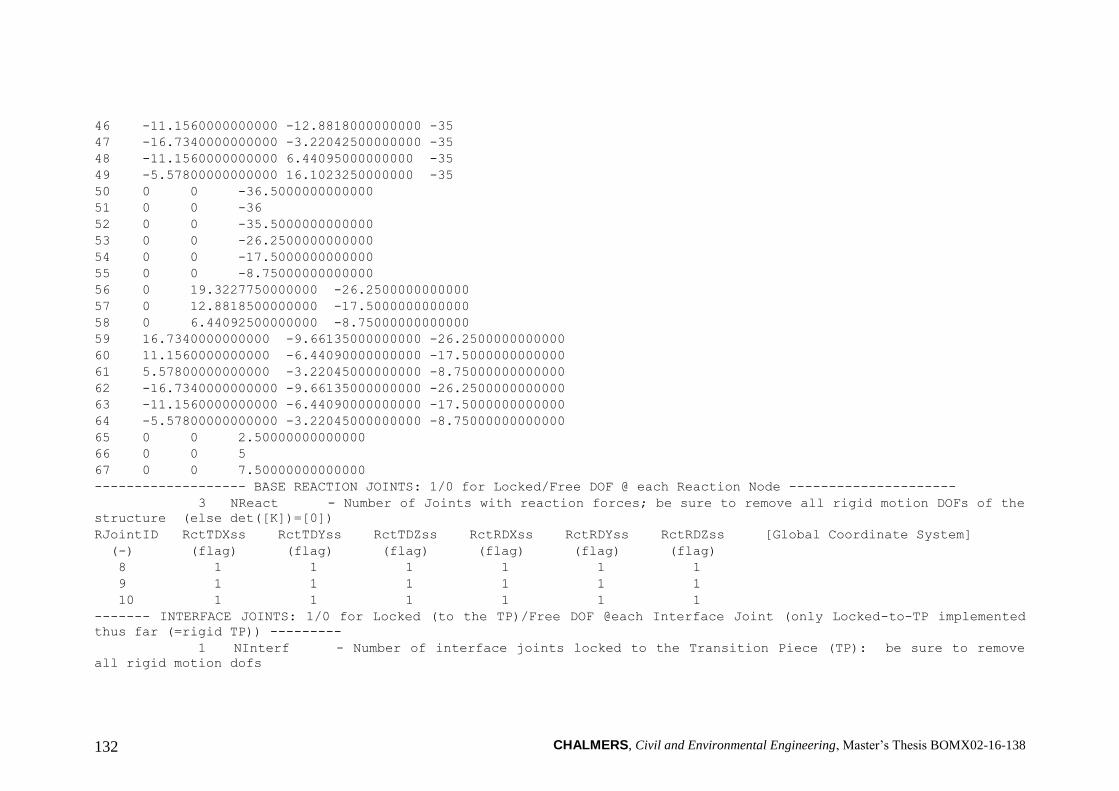
CHALMERS, Civil and Environmental Engineering, Master’s Thesis BOMX02-16-138 132
46 -11.1560000000000 -12.8818000000000 -35
47 -16.7340000000000 -3.22042500000000 -35
48 -11.1560000000000 6.44095000000000 -35
49 -5.57800000000000 16.1023250000000 -35
50 0 0 -36.5000000000000
51 0 0 -36
52 0 0 -35.5000000000000
53 0 0 -26.2500000000000
54 0 0 -17.5000000000000
55 0 0 -8.75000000000000
56 0 19.3227750000000 -26.2500000000000
57 0 12.8818500000000 -17.5000000000000
58 0 6.44092500000000 -8.75000000000000
59 16.7340000000000 -9.66135000000000 -26.2500000000000
60 11.1560000000000 -6.44090000000000 -17.5000000000000
61 5.57800000000000 -3.22045000000000 -8.75000000000000
62 -16.7340000000000 -9.66135000000000 -26.2500000000000
63 -11.1560000000000 -6.44090000000000 -17.5000000000000
64 -5.57800000000000 -3.22045000000000 -8.75000000000000
65 0 0 2.50000000000000
66 0 0 5
67 0 0 7.50000000000000
------------------- BASE REACTION JOINTS: 1/0 for Locked/Free DOF @ each Reaction Node ---------------------
3 NReact - Number of Joints with reaction forces; be sure to remove all rigid motion DOFs of the
structure (else det([K])=[0])
RJointID RctTDXss RctTDYss RctTDZss RctRDXss RctRDYss RctRDZss [Global Coordinate System]
(-) (flag) (flag) (flag) (flag) (flag) (flag)
8 1 1 1 1 1 1
9 1 1 1 1 1 1
10 1 1 1 1 1 1
------- INTERFACE JOINTS: 1/0 for Locked (to the TP)/Free DOF @each Interface Joint (only Locked-to-TP implemented
thus far (=rigid TP)) ---------
1 NInterf - Number of interface joints locked to the Transition Piece (TP): be sure to remove
all rigid motion dofs

CHALMERS, Civil and Environmental Engineering, Master’s Thesis BOMX02-16-138 133
IJointID ItfTDXss ItfTDYss ItfTDZss ItfRDXss ItfRDYss ItfRDZss [Global Coordinate System]
(-) (flag) (flag) (flag) (flag) (flag) (flag)
12 1 1 1 1 1 1
----------------------------------- MEMBERS --------------------------------------
72 NMembers - Number of frame members
MemberID MJointID1 MJointID2 MPropSetID1 MPropSetID2 COSMID
(-) (-) (-) (-) (-) (-)
1 1 14 1 1
2 14 15 2 2
3 15 16 3 3
4 16 4 4 4
5 2 17 5 5
6 17 18 6 6
7 18 19 7 7
8 19 4 8 8
9 3 20 9 9
10 20 21 10 10
11 21 22 11 11
12 22 4 12 12
13 1 23 13 13
14 23 24 14 14
15 24 25 15 15
16 25 5 16 16
17 2 26 17 17
18 26 27 18 18
19 27 28 19 19
20 28 6 20 20
21 3 29 21 21
22 29 30 22 22
23 30 31 23 23
24 31 7 24 24
25 8 32 25 25
26 32 33 26 26

CHALMERS, Civil and Environmental Engineering, Master’s Thesis BOMX02-16-138 134
27 33 34 27 27
28 34 1 28 28
29 9 35 29 29
30 35 36 30 30
31 36 37 31 31
32 37 2 32 32
33 10 38 33 33
34 38 39 34 34
35 39 40 35 35
36 40 3 36 36
37 1 41 37 37
38 41 42 38 38
39 42 43 39 39
40 43 2 40 40
41 2 44 41 41
42 44 45 42 42
43 45 46 43 43
44 46 3 44 44
45 3 47 45 45
46 47 48 46 46
47 48 49 47 47
48 49 1 48 48
49 13 50 49 49
50 50 51 50 50
51 51 52 51 51
52 52 4 52 52
53 4 53 53 53
54 53 54 54 54
55 54 55 55 55
56 55 11 56 56
57 1 56 57 57
58 56 57 58 58
59 57 58 59 59

CHALMERS, Civil and Environmental Engineering, Master’s Thesis BOMX02-16-138 135
60 58 11 60 60
61 2 59 61 61
62 59 60 62 62
63 60 61 63 63
64 61 11 64 64
65 3 62 65 65
66 62 63 66 66
67 63 64 67 67
68 64 11 68 68
69 11 65 69 69
70 65 66 70 70
71 66 67 71 71
72 67 12 72 72
------------------ MEMBER X-SECTION PROPERTY data 1/2 [isotropic material for now: use this table for circular-
tubular elements] ------------------------
72 NPropSets - Number of structurally unique x-sections (i.e. how many groups of X-sectional
properties are utilized throughout all of the members)
PropSetID YoungE ShearG MatDens XsecD XsecT
(-) (N/m2) (N/m2) (kg/m3) (m) (m)
1 210000000000.000 81000000000.0000 7850 0.800000000000000 0.0280000000000000
2 210000000000.000 81000000000.0000 7850 0.800000000000000 0.0280000000000000
3 210000000000.000 81000000000.0000 7850 0.800000000000000 0.0280000000000000
4 210000000000.000 81000000000.0000 7850 0.800000000000000 0.0280000000000000
5 210000000000.000 81000000000.0000 7850 0.800000000000000 0.0280000000000000
6 210000000000.000 81000000000.0000 7850 0.800000000000000 0.0280000000000000
7 210000000000.000 81000000000.0000 7850 0.800000000000000 0.0280000000000000
8 210000000000.000 81000000000.0000 7850 0.800000000000000 0.0280000000000000
9 210000000000.000 81000000000.0000 7850 0.800000000000000 0.0280000000000000
10 210000000000.000 81000000000.0000 7850 0.800000000000000 0.0280000000000000
11 210000000000.000 81000000000.0000 7850 0.800000000000000 0.0280000000000000
12 210000000000.000 81000000000.0000 7850 0.800000000000000 0.0280000000000000
13 210000000000.000 81000000000.0000 7850 4 0.0400000000000000
14 210000000000.000 81000000000.0000 7850 4 0.0400000000000000

CHALMERS, Civil and Environmental Engineering, Master’s Thesis BOMX02-16-138 136
15 210000000000.000 81000000000.0000 7850 4 0.0400000000000000
16 210000000000.000 81000000000.0000 7850 4 0.0400000000000000
17 210000000000.000 81000000000.0000 7850 4 0.0400000000000000
18 210000000000.000 81000000000.0000 7850 4 0.0400000000000000
19 210000000000.000 81000000000.0000 7850 4 0.0400000000000000
20 210000000000.000 81000000000.0000 7850 4 0.0400000000000000
21 210000000000.000 81000000000.0000 7850 4 0.0400000000000000
22 210000000000.000 81000000000.0000 7850 4 0.0400000000000000
23 210000000000.000 81000000000.0000 7850 4 0.0400000000000000
24 210000000000.000 81000000000.0000 7850 4 0.0400000000000000
25 210000000000.000 81000000000.0000 7850 4 0.0400000000000000
26 210000000000.000 81000000000.0000 7850 4 0.0400000000000000
27 210000000000.000 81000000000.0000 7850 4 0.0400000000000000
28 210000000000.000 81000000000.0000 7850 4 0.0400000000000000
29 210000000000.000 81000000000.0000 7850 4 0.0400000000000000
30 210000000000.000 81000000000.0000 7850 4 0.0400000000000000
31 210000000000.000 81000000000.0000 7850 4 0.0400000000000000
32 210000000000.000 81000000000.0000 7850 4 0.0400000000000000
33 210000000000.000 81000000000.0000 7850 4 0.0400000000000000
34 210000000000.000 81000000000.0000 7850 4 0.0400000000000000
35 210000000000.000 81000000000.0000 7850 4 0.0400000000000000
36 210000000000.000 81000000000.0000 7850 4 0.0400000000000000
37 210000000000.000 81000000000.0000 7850 0.800000000000000 0.0160000000000000
38 210000000000.000 81000000000.0000 7850 0.800000000000000 0.0160000000000000
39 210000000000.000 81000000000.0000 7850 0.800000000000000 0.0160000000000000
40 210000000000.000 81000000000.0000 7850 0.800000000000000 0.0160000000000000
41 210000000000.000 81000000000.0000 7850 0.800000000000000 0.0160000000000000
42 210000000000.000 81000000000.0000 7850 0.800000000000000 0.0160000000000000
43 210000000000.000 81000000000.0000 7850 0.800000000000000 0.0160000000000000
44 210000000000.000 81000000000.0000 7850 0.800000000000000 0.0160000000000000
45 210000000000.000 81000000000.0000 7850 0.800000000000000 0.0160000000000000
46 210000000000.000 81000000000.0000 7850 0.800000000000000 0.0160000000000000
47 210000000000.000 81000000000.0000 7850 0.800000000000000 0.0160000000000000

CHALMERS, Civil and Environmental Engineering, Master’s Thesis BOMX02-16-138 137
48 210000000000.000 81000000000.0000 7850 0.800000000000000 0.0160000000000000
49 210000000000.000 81000000000.0000 7850 4 0.0280000000000000
50 210000000000.000 81000000000.0000 7850 4.02702500000000 0.0285500000000000
51 210000000000.000 81000000000.0000 7850 4.05405000000000 0.0291000000000000
52 210000000000.000 81000000000.0000 7850 4.08107500000000 0.0296500000000000
53 210000000000.000 81000000000.0000 7850 4.10810000000000 0.0302000000000000
54 210000000000.000 81000000000.0000 7850 4.58107500000000 0.0396500000000000
55 210000000000.000 81000000000.0000 7850 5.05405000000000 0.0491000000000000
56 210000000000.000 81000000000.0000 7850 5.52702500000000 0.0585500000000000
57 210000000000.000 81000000000.0000 7850 1.20000000000000 0.0320000000000000
58 210000000000.000 81000000000.0000 7850 1.20000000000000 0.0320000000000000
59 210000000000.000 81000000000.0000 7850 1.20000000000000 0.0320000000000000
60 210000000000.000 81000000000.0000 7850 1.20000000000000 0.0320000000000000
61 210000000000.000 81000000000.0000 7850 1.20000000000000 0.0320000000000000
62 210000000000.000 81000000000.0000 7850 1.20000000000000 0.0320000000000000
63 210000000000.000 81000000000.0000 7850 1.20000000000000 0.0320000000000000
64 210000000000.000 81000000000.0000 7850 1.20000000000000 0.0320000000000000
65 210000000000.000 81000000000.0000 7850 1.20000000000000 0.0320000000000000
66 210000000000.000 81000000000.0000 7850 1.20000000000000 0.0320000000000000
67 210000000000.000 81000000000.0000 7850 1.20000000000000 0.0320000000000000
68 210000000000.000 81000000000.0000 7850 1.20000000000000 0.0320000000000000
69 210000000000.000 81000000000.0000 7850 6 0.0400000000000000
70 210000000000.000 81000000000.0000 7850 6 0.0400000000000000
71 210000000000.000 81000000000.0000 7850 6 0.0400000000000000
72 210000000000.000 81000000000.0000 7850 6 0.0400000000000000
------------------ MEMBER X-SECTION PROPERTY data 2/2 [isotropic material for now: use this table if any section
other than circular, however provide COSM(i,j) below] ------------------------
0 NXPropSets - Number of structurally unique non-circular x-sections (if 0 the following table is
ignored)
PropSetID YoungE ShearG MatDens XsecA XsecAsx XsecAsy XsecJxx
XsecJyy XsecJ0
(-) (N/m2) (N/m2) (kg/m3) (m2) (m2) (m2) (m4)
(m4) (m4)
---------------------- MEMBER COSINE MATRICES COSM(i,j) ------------------------
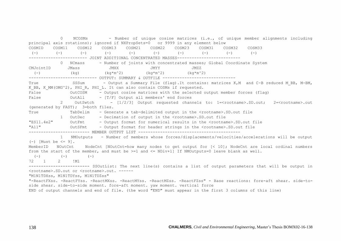
CHALMERS, Civil and Environmental Engineering, Master’s Thesis BOMX02-16-138 138
0 NCOSMs - Number of unique cosine matrices (i.e., of unique member alignments including
principal axis rotations); ignored if NXPropSets=0 or 9999 in any element below
COSMID COSM11 COSM12 COSM13 COSM21 COSM22 COSM23 COSM31 COSM32 COSM33
(-) (-) (-) (-) (-) (-) (-) (-) (-) (-)
------------------------ JOINT ADDITIONAL CONCENTRATED MASSES--------------------------
0 NCmass - Number of joints with concentrated masses; Global Coordinate System
CMJointID JMass JMXX JMYY JMZZ
(-) (kg) (kg*m^2) (kg*m^2) (kg*m^2)
---------------------------- OUTPUT: SUMMARY & OUTFILE ------------------------------
True SSSum - Output a Summary File (flag).It contains: matrices K,M and C-B reduced M_BB, M-BM,
K_BB, K_MM(OMG^2), PHI_R, PHI_L. It can also contain COSMs if requested.
False OutCOSM - Output cosine matrices with the selected output member forces (flag)
False OutAll - [T/F] Output all members' end forces
2 OutSwtch - [1/2/3] Output requested channels to: 1=<rootname>.SD.out; 2=<rootname>.out
(generated by FAST); 3=both files.
True TabDelim - Generate a tab-delimited output in the <rootname>.SD.out file
1 OutDec - Decimation of output in the <rootname>.SD.out file
"ES11.4e2" OutFmt - Output format for numerical results in the <rootname>.SD.out file
"A11" OutSFmt - Output format for header strings in the <rootname>.SD.out file
------------------------- MEMBER OUTPUT LIST ------------------------------------------
1 NMOutputs - Number of members whose forces/displacements/velocities/accelerations will be output
(-) [Must be <= 9].
MemberID NOutCnt NodeCnt [NOutCnt=how many nodes to get output for [< 10]; NodeCnt are local ordinal numbers
from the start of the member, and must be >=1 and <= NDiv+1] If NMOutputs=0 leave blank as well.
(-) (-) (-)
72 1 2 !M1
------------------------- SSOutList: The next line(s) contains a list of output parameters that will be output in
<rootname>.SD.out or <rootname>.out. ------
"M1N1TDXss, M1N1TDYss, M1N1TDZss"
"-ReactFXss. -ReactFYss. -ReactMXss. -ReactMYss. -ReactMZss. -ReactFZss" - Base reactions: fore-aft shear. side-to-
side shear. side-to-side moment. fore-aft moment. yaw moment. vertical force
END of output channels and end of file. (the word "END" must appear in the first 3 columns of this line)


![Databaseforahighperformanceandstability demanding command ...publications.lib.chalmers.se/records/fulltext/127516.pdf · Chapter 1 Introduction TraditionallySaab[3]hasstoredapplicationdatainadistributeddatastructure](https://img.dokumen.tips/doc/110x75/5f283e290d51ca22422dad96/databaseforahighperformanceandstability-demanding-command-chapter-1-introduction.jpg)


![Thesis Report Final[1] - Chalmers Publication Library (CPL)publications.lib.chalmers.se/records/fulltext/156053.pdf · TableofContents’ Acknowledgements](https://img.dokumen.tips/doc/110x75/5a9dbda47f8b9a96438beebd/thesis-report-final1-chalmers-publication-library-cpl-acknowledgements.jpg)

