Pedestrian Detection Using Structured SVM

Wonhui KimStanford University

Department of Electrical Engineeringwonhui@stanford.edu

Seungmin LeeStanford University

Department of Electrical Engineeringsmlee729@stanford.edu

1. Introduction

With the advent of smart car and even driverless cars, theimportance of intelligent driver’s system has been rapidlygrowing. Accordingly, driver’s vision has become one ofthe most popular issues and especially detecting some ob-stacles and pedestrians on the road are at the center of thevision problem in order to prevent accidents. Motivated bythe importance of such topics, we implemented the humandetector in the project.

Our approach is based on Deformable Part Model[1],one of the most powerful method for object detection. Inthe learning part of the system, we applied Structured SVM(SSVM) instead of Latent SVM (LSVM) which is used in[1]. The major goal of this project is not only to understandhow differnt types of SVM can work on the detection prob-lem but also to apply SSVM on our pedestrian detectionproblem.

Related Work

Dalal and Triggs[7] have developed the idea of his-togram of gradient and have achieved excellent recognitionrate of human detection in images. They used the conceptsof HOG and designed a baseline classifier using a linearSVM. After a few years, Felzenszwalb et al. [1] introducedthe deformable part model applying latent SVM. The per-formance of the detector has been significantly improvedby combining HOG feature pyramid with deformable partmodel. Deformable part model has been applied in vari-ous papers and it is considered as the most general frame-work for object detection in 2D image. In [3], the conceptof structured SVM first introduced, whose major differencefrom previous ones is the structured vector form of the out-put and the loss rescaling in the constraint inequality. The-oretical background of our project is mainly based on thoseworks.

Overview

Our detection method is summarized in two phases: thelearning phase and the detection phase.

Figure 1. Overview block diagram.

During the whole procedure, we do not use raw imagesbut instead use transformed images into HOG feature space.Since our approach is mainly based on the window scan-ning, HOG feature pyramid with different levels is con-structed for each image.

The model mainly consists of root filter and part filterswhich should be obtained after the completion of the learn-ing process. Root filter is trained with the coarse resolutionwhereas part filters are trained with finer resolution. Usingthe SSVM learning algorithm and given annotation files forthe training data which contains ground-truth bounding boxcoordinates, the optimal root filter and part filters can beobtained.

With obtained root and part filters, the scores for eachtest image are calculated by taking the convolution betweenthe filters and the HOG feature pyramid of an image. Thenwe will determine whether some parts of image are desiredobjects or not based on the given threshold. Finally, wewill use precision-recall curve and average precision(AP)to evaluate our model.

2. Deformable Part Model

2.1. Learning

A model is defined as (F0, P1, ..., Pn, b) which consistsof a root filter F0, n numbers of part models P1, ..., Pn, andthe real-valued bias term b. Each part model Pi consistsof a part filter Fi, the location ui relative to the root filter

1

and the coefficients vector di for evaluating the deformationcost. The ultimate goal of learning is to find the optimal pa-rameters vector w = (F0, P1, ..., Pn, b). More details ofparameter settings are in [1]. The primal optimization prob-lem of latent SVM with soft margin can be simplified asfollows.

minw,ξ

1

2‖w‖2 + C

m∑i=1

ξi

s.t.∀i ∈ {1, ...,m} ξi ≥ 0,

y(i)hw(x(i)) ≥ 1− ξi

where y(i) ∈ {−1, 1}. It looks identical to the linear SVMbut the difference is in the definition of hypothesis functionwhich involves some latent variables.

hw(x) = maxz∈Z(x)

wTφ(x, z)

Z(x) denotes latent domain of valid placements for the rootand part filters specified by x. Latent variable z ∈ Z(x)contains latent information about the relative part locationsand the whole configuration. Φ(x, z) is the concatenationof features for the root filter, part filters, deformation cost,and the constant 1 for the bias term.

2.2. Detection

A model obtained through training is defined as(F0, P1, ..., Pn, b) where F0 is a root filter, Pi is the i-th partmodel and b is a scalar bias term. Each part model consistsof a part filter Fi, the relative location to the root filter uiand the coefficient vector for evaluating a deformation costfor each possible placement of the part.

With learned filter parameters (F0, P1, ..., Pn, b) and thefeature pyramid which is calculated with a new input im-age x as a part of scanning window approach, we can nowimplement the detection by evaluating their dot product as ascore. By thresholding the scores for all root filter locations,we can finally detect people in a test image.

2.3. Multi-Component Model

In practice, there are some variations in human imagesdue to different poses, directions and actions. Therefore,defining only a single model for the human detector wouldprove ineffective for such images. Instead of constructinga single model, we split the whole positive training imagesinto N groups according to aspect ratio, the ratio betweenthe width and the height of bounding boxes, and then con-struct models for each group.

In this project, we trained models for both 1 componentand 2 component cases since human images do not containmuch variations compared to other objects.

3. Structured SVMBoth linear SVM and latent SVM are binary classifiers

where target variable y is binary. Rather than predictinga binary label for each input, SSVM predicts structuredresponses. Given m training examples {(x(i), y(i))} fori=1,...m, where x denotes the feature vector extracted fromith training image and y is the structured output, the SSVMoptimizes w by minimizing a quadratic objective functionsubject to a set of linear inequality constraints:

minw,ξ

1

2‖w‖2 +

C

m

m∑i=1

ξi s.t.∀i ∈ {1, ...,m},

∀y ∈ Y \yi : 〈w, δΨi(y)〉 ≥ 4(yi, y)− ξiThere are m(|Y | − 1) numbers of inequalities where w

is a parameter vector, Y \yi is the set of possible outputsexcluding yi and ξi is a non-negative slack variable for ith

example. δΨi(y) = Ψ(xi, yi) − Ψ(xi, y) where Ψ(x, y)represents some combined feature representation of inputsand outputs and4(yi, y) is a loss function.

With the parameter vector w obtained, we can make aprediction by maximizing the score function F over the re-sponse variable for a specific given input x as follows.

hw(x) = argmaxy∈Y

F (x, y;w)

where F (x, y;w) = 〈w,Ψ(x, y)〉One of the major advantages of applying SSVM is tun-

ability to specific loss functions. We call this margin rescal-ing, creating larger margins for the classes of most desirablemisclassification. By defining the loss function4(yi, y) asany appropriate form that is in general proportional to thedissimilarity between two outputs, we can give flexibility tothe inequality thereby performing better training comparedto the case when just using a constant loss.

4. ExperimentBefore implementing our human detector, many things

must be decided such as features, parameters, loss functionsfor SSVM, optimization algorithm, training dataset, and soon. In this section, we focus more on practical issues suchas how we specified some important variables and look intothe details for the implementation.

4.1. Data Selection

PASCAL VOC 2012 dataset which contains 23,080training examples with complete annotations is used for theproject. For each image, xml file is provided, which con-tains class label and ground-truth bounding box positionsbut not for part locations.

It also has images for testing but does not contain a com-plete set of data labelling files, so we evaluated our systemusing 9,963 test images from PASCAL VOC 2007 dataset.

2

4.2. Feature Selection: HOG Descriptor

The accuracy and the effectiveness of HOG feature forhuman detection has been verified in many works and iscurrently accepted as one of the most appropriate and gen-eralized feature. We also use HOG feature for this project.More details are in [7].

When applying HOG feature transformation to an image,we obtain 36 transformed images for each gradient orienta-tion and normalization. Due to the window scanning ap-proach applied in this project, we use the concept of HOGfeature pyramid instead. With various resolutions of an im-age, we calculate HOG features for each level of resolution.

4.3. Parameters Setting

Before applying SSVM algorithm to our problem, inputand output vectors and also the parameters vector should beclarified. The two most distinctive characteristics of SSVMis the flexibility in choosing loss functions and the form ofoutputs which can be a structured vector form. We choosethe output vector as y = (yl, yb) where yl ∈ {1,−1} andyb is a four dimensional bounding box labels vector.

4.4. The Loss Function

We can simply choose the loss function for this y and itsground-truth vector y(i) as follows.

4(y, y(i)) = 1− o(yb, y(i)b ) if yl = y(i)l = 1

where o(yb, y(i)b ) is the fraction of overlap area defined by

two vectors. Overlap area is computed by dividing the areaof intersection as the union of two vectors.

As a possible output y approaches the true output y(i),o(yb, y

(i)b ) gets larger thus the loss decreases. With lower

values of loss, it would become easy to satisfy the con-straint. Thus, the flexibility of the loss function increasesthe probability to satisfy the constraint for outputs that areclose to the ground-truth output. On the other hand, if yand y(i) do not overlap, the loss is maximized with value 1.Since the bound of inequality constraint is more strict, it be-comes more likely to violate the constraint. Thus, the flexi-bility of the loss function decreases the probability to satisfythe constraint for outputs that are far from the ground-truthoutput.

For negative images, y does not have ground-truthbounding boxes, hence we just use 1 for the loss. In thecode implementation, we do not face with the case where yland y(i)l are different, so we do not have to define the lossmore in specific for such cases.

4.5. Implementation Detail

As in [1], we train the SSVM using the coordinate de-scent approach together with the datamining and gradientdescent algorithm.

When performing the coordinate descent, we first findthe latent variable z(i) for each training example, whichmaximizes the score calculated with the fixed parametervector w. That is, for every m training examples, find rootand part filter locations z(i) around x(i) having the maxi-mum score.

z(i) = argmaxz∈Z(x(i))

wTφ(x(i), z)

After the completion of the first step, we find the pa-rameters vector w using the stochastic gradient descent.When updating the parameters vector, we can apply the lossfunction when checking the satisfiability of inequality con-straints.

As for the negative training examples, it should be care-fully chosen for the parameter update. Since there are ahuge amount of possible negative examples, we performdatamining hard negatives which are relatively close to thescore of positive examples so misclassified as positive butactually they are negative.

The real implementation does not exactly follow the def-inition of SSVM. For positive examples, instead of updat-ing the parameter vectors for all the possible locations ofbounding boxes, we first choose z(i), the latent variablewhich maximizes the score, with calculating its overlap areao(z(i), y

(i)b ) because otherwise the computation is too ex-

pensive. Then, we perform learning with such optimal z(i)

by checking whether the constraint satisfied or not accord-ing to the value of o(z(i), y(i)b ).

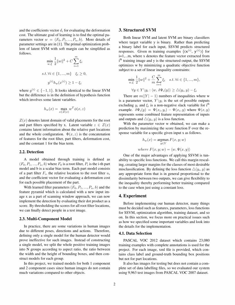
5. Results

5.1. Trained Model

We constructed both one and two component models forhuman detector. Figure 2 and figure 3 shows the resultingmodels learned on PASCAL VOC 2012 dataset. 6 parts areused when learning, but we can see that one of them doesnot take the important role in the person model.

5.2. Evaluation

Since PASCAL VOC 2012 dataset does not contain acomplete set of data labellings, we evaluated our systemusing 9,963 test images from PASCAL VOC 2007 dataset.The dataset specify ground-truth bounding boxes of humanlocation for each image. Based on the calculated scores foreach image, we can evaluate the precision and the recall.The precision is the number of true positives divided by thetotal number of elements labeled as belonging to the pos-itive class, and the recall is the number of true positivesdivided by the total number of elements that actually be-long to the positive class. In other words, the precision isthe fraction of the reported bounding boxes that are correct

3

Figure 2. 1-component person model obtained by SSVM. This sin-gle model cannot generalize various shapes of person in randomtest images.

Figure 3. 2-component person model obtained by SSVM. Uppermodel showing fat-shaped person seems to represent those whoare sitting down. Bottom model shows normal shape of person.

detections, while recall is the fraction of the objects foundcorrectly.

Figure 4 shows the precision/recall curves for four differ-ent learning procedure. As we can see from the figure, thecurves resulting from SSVM is closer to the top right sideof the plot than those from LSVM. More specific values arein figure 5.

Depending on the determination method for final bound-ing boxes, we have two kind of measures. While Test1 col-umn indicates the result only considered root location, Test2column shows the result considered both root and part loca-tions. Average precisions(AP) resulting from SSVM learn-ing are greater than those from LSVM learning for both 1-component and 2-component models. Especially as for the2-component model, we have achieved roughly 4% of theperformance improvement compared to the original humandetector based on LSVM learning algorithm.

Figure 4. Comparison of precision/recall curves between the mod-els obtained using LSVM and SSVM. The more the curve is placedon the top right side of the plane, the better the detector is.

Figure 5. Comparison of LSVM and SSVM with average preci-sions. N is the number of components of the model, and Test1 andTest2 use slightly different algorithm to decide the final boundingboxes position. Regardless of which test used, SSVM always givesbetter performance than LSVM.

6. Conclusion

In this project, we have applied SSVM to the humandetection problem based on deformable part model. Theoptimization problem for SSVM is solved though coordi-nate descent technique, which involves datamining hardnegatives and stochastic gradient descent. As a result, weachieved roughly 4% of performance improvement for the2-component human detector. That is because SSVM givesflexibility to choose the loss function, making the constrainttough for examples far from the ground-truth one whilemake it loose for those close to the ground-truth vector thusraising the possibility to satisfy the constraint.

4

Figure 6. Detection examples using deformable part model learnedby SSVM. It is actually hard to detect the difference between re-sulting images from LSVM and SSVM through the eye, SSVMshows better performance. Images on the left column shows rootbounding boxes together with each part, and images on the rightcolumn shows the final bounding boxes.

7. Future Work

Due to the heavy load of computation, especially dur-ing the learning procedure, we only performed the detectionfor human. However, our approach can be generalized forother object classes as well, such as vehicles, animals andso forth. In such a case, however, another type of featuresinstead of HOG feature might have to be chosen.

In addition, it would be possible to apply the com-plete SSVM learning which exactly follows the optimiza-tion problem mentioned in section 3 in the implemenationprocedure. In this project we only focused on the lossrescaling of SSVM and defined the loss function in a re-ally simple form, but there might be more effective wayto design the structured output vector y at the expense ofheavier computation. So we are now planning to design thelearning parameters in a different way that leads to betterperformance.

References

[1] P. Felzenszwalb, D. McAllester, D. Ramanan, ”Adiscriminatively trained, multiscale, deformable partmodel”. CVPR, 2008.

[2] P. Felzenszwalb, R. Girshick, D. McAllester, D. Ra-manan, ”Object detection with discriminatively trainedpart based models”. PAMI, 2010.

[3] I. Tsochantaridis, T. Joachims, T. Hofmann, Y. Altun,”Large margin methods for structured and interdepen-dent output variables”. JMLR, 2005.

[4] B. Pepik, M. Stark, P. Gehler and B. Schiele, ”Teaching3D geometry to deformable part models”. CVPR, 2012.

[5] M. Blaschko, C. Lampert, ”Learning to localize objectswith structured output regression”. ECCV, 2008.

[6] , C. Desai, D. Ramanan, C. Fowlkes, ”Discriminativemodels for multi-class object layout”. ICCV, 2009.

[7] , N. Dalal, B. Triggs, ”Histogram of Oriented Gradientsfor Human Detection”. CVPR, 2005.

5