Supplementary Figures 

 

Supplementary Figure 1 | Preparation of LCE microparticles. Bulk LCE specimen are freeze‐fractured into μLCE powder. 

Depending on the nematic domain order in the bulk, which can be either “single crystal”‐like, e.g. monodomain (panel a top), 

polydomain with domain size  dL  of the order of the μLCE size  cL  (panel b top), or polydomain with domains much smaller than 

μLCE particles (panel c top), the resulting μLCEs are monodomain grains in the first case (panel a bottom), monodomain or low domain count grains in the second case (panel b bottom), and polydomain grains in the third case (panel c bottom). 

polydomain

bulk LCE, Ld << Lc

≈Ld

≈Lc

polydomain

bulk LCE, Ld ≈Lc

≈Ld

≈Lc

monodomain

bulk LCE, Ld >> Lc

Ld →∞

≈Lc

a cb

 

Supplementary Figure 2 | Time evolution of LCE microparticles' orientational order parameter. Theoretical  ( / )Q t t τ  

profile is calculated from equation (13) of Supplementary Note 2.  

 

Supplementary Figure 3 | Sketch of the deformation of layer geometry on heating. a, “Series” scenario. b, “Parallel” scenario. The shape of the PDLCE specimen is shown below  λT  as a blue wireframe and above  λT  as a red wireframe. LCE and PDMS 

layers are shaded in light yellow and light green, respectively. The unconstrained shape (disregarded internal stress) is shown in magenta colour (panel b bottom right). 

hea�ng

T0 << Tλ Tref >> Tλ

parallel

L p(T

ref)

L p(T

0)

E p ,

λ p(T

)

l p(T r

ef)∝

L p(T

ref)

l’ LCE(T

ref)

l’ PDM

S(T

ref)

l LCE(T

ref)

=l PD

MS(T

ref)

l p(T 0

)∝L p

(T0)

l LCE(T

0)=

l PDM

S(T

0)

F

-F

-F

F

nn

hea�ng

T0 << Tλ Tref >> Tλ

seriesE s

, λ s

(T )

L s(T

ref)

L s(T

0)

l s(T r

ef)∝

L s(T

ref)

l LCE(T

ref)

l PDM

S(T

ref)

l s(T 0

)∝L s

(T0)

l LCE(T

0)

l PDM

S(T

0)

nn

a b

 

Supplementary Figure 4 | PDLCE performance. The effective thermomechanical response  p room( )λ T  depends on the nematic 

order parameter  S  of μLCE particles at the setting temperature  0 .T  Consecutive curves correspond to  LCE PDMS/y E E 0, 0.2, 

0.4, 0.6, 0.8 and 1 (bottom to top), all calculated with  0.45γ  and  0.5,ν  with two different values of the μLCE orientational 

order parameter,  1Q  for ideal alignment (blue solid lines) and  0.8Q  for partially disordered alignment (red dashed line).  

 

p

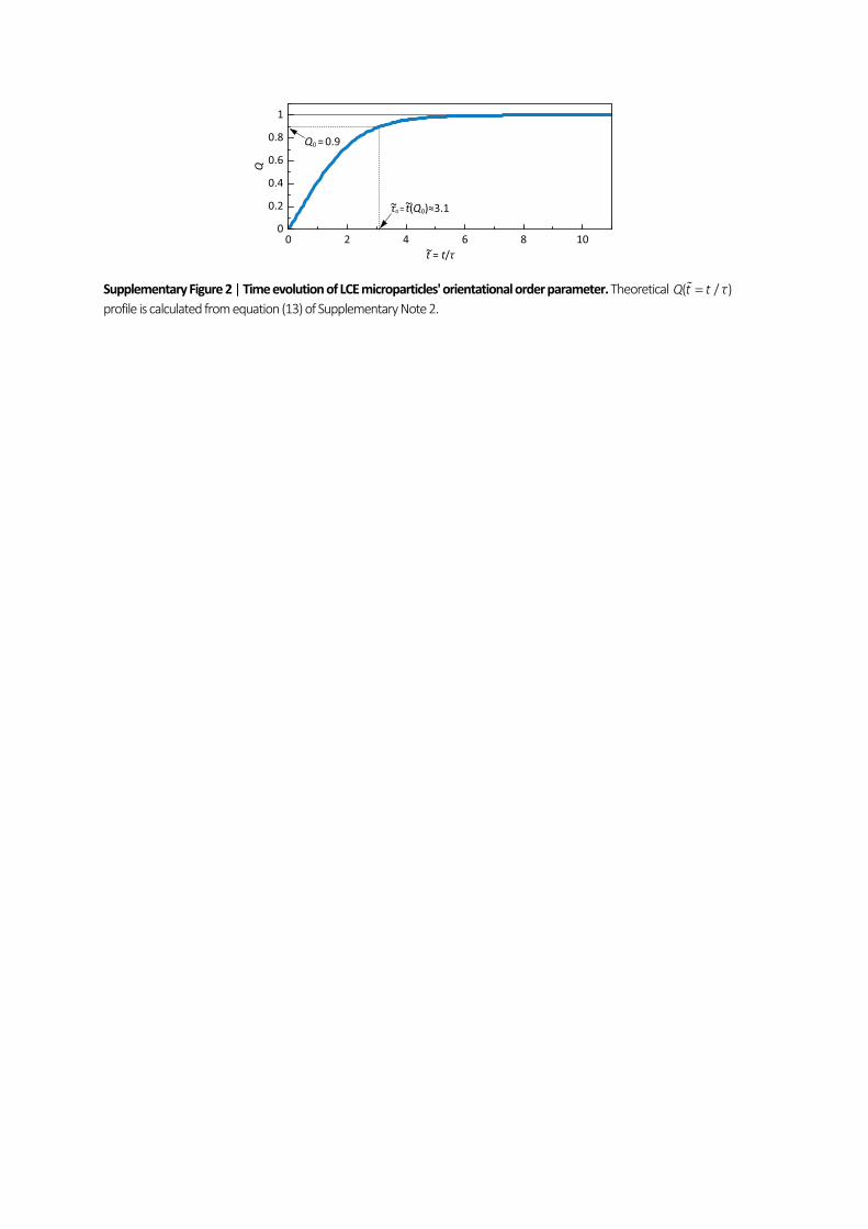
Supplementary Note 1 | Nematic domains in μLCEs 

LCE microparticles, fabricated from fully ordered bulk LCEs, specifically from LCE-A, LCE-B1, and LCE-B2, are nematic monodomains (Supplementary Fig. 1), described as “mono” in Table 1. Crushing of polydomain bulk LCE materials (LCE-Ap and LCE-Cp), on the other hand, results in either polydomain or monodomain μLCEs (described as “poly/mono” in Table 1), depending on the actual size of microparticles (Supplementary Figs. 1b, c). In our case, typical sizes of μLCE and nematic domains both span the range of several microns to a few ten microns, so that μLCEs produced from polydomain bulk material consist of several misaligned nematic domains (Supplementary Fig. 1b) with small but non-zero residual effective nematic order .S In the partially ordered LCE-C, manufactured with magnetic field-assisted crosslinking, nematic domains are large enough for the freeze-fracturing to result in prevalently monodomain microsized LCE particles, with large residual ,S irrespective of domain order of the bulk material. LCE-C thus serves equally well as the fully ordered bulk material like LCE-A in the production of monodomain μLCEs.

Supplementary Note 2 | Magnetic alignment

Orientational order of μLCEs. We shall assume that μLCE grains are ideal uniaxial nematic

monodomains, so that their orientation is given by the angle , n Z between the nematic director n

and the Z axis of the laboratory frame. The orientational distribution (cos )P of μLCE grains, which

is isotropic in the prepolymer mixture, 0 (cos ) 1,P becomes increasingly anisotropic when LCE

microparticles are aligned in the external magnetic field,

0 0

1

0

cos cos cos , cos cos .tP t d (1)

Here t measures the time since the start of aligning and denotes the Dirac's delta function. Relation

0cos ( , cos ),t which is obtained by solving the equation of motion, measures the alignment of a given

LCE microparticle with its nematic director initially oriented at 0 ( , ) n B Z at time 0.t We have

taken into account that, during the aligning, (cos )tP remains (i) cylindrically symmetric, i.e.

independent of azimuthal angle , about B and (ii) invariant to the transformation , allowing

for restriction of tilt angle definition range to [cos 0 .],1 The orientational order is commonly

quantified by the orientational order parameter 2(3cos 1) / 2,Q with the average performed over

(cos )P (Supplementary Ref. 1). In our specific case, taking into account equation (1), we obtain

1

20 0

0

13 cos , cos 1 cos .

2Q t dt (2)

PDLCEs can thus be simply characterized in terms of ,Q which quantifies the orientational order of

μLCEs. For PDLCE composites, cured in the external field ,B full alignment ( 1)Q or partial

alignment (0 1)Q is achieved in the respective cases of monodomain or polydomain μLCEs. On the

other hand, during zero field curing, LCE microparticles remain isotropically distributed ( 0),Q therefore we label this state as “iso” (Table 2). Consistently, PDLCE specimens with 0Q exhibit

macroscopically observable thermomechanical response, whereas PDLCE specimens with 0Q are

thermomechanically inert (Fig. 2).

Equation of reorientational motion. LCE microparticles are treated as diamagnetically anisotropic, nematic monodomain ellipsoidal objects. Their alignment is driven by the magnetic torque

2

0

1sin cosB VS B

(3)

and viscous torque

38.

r d

F r R dt

(4)

Here 0 denotes the magnetic permeability of the vacuum, V the volume of the microparticle, S the

nematic order parameter, the anisotropy of diamagnetic susceptibility, ( , ) n B the angle between

the nematic director n and magnetic field B , and the viscosity of the uncured matrix. r and R are

the radii of the short and long axis of the ellipsoid, respectively. The geometrical factor ( / )F r R equals

1 for a sphere ( / 1)r R and exhibits only a modest decrease for moderately deformed sphere, e.g.

(0.5) 0.9,F (2) 0.7F (Supplementary Ref. 2). Since our particular LCE microparticles resemble

spheres rather than rods or discs, we accordingly approximate 1.r R F The equation of motion then reads

2

2.B

dI

dt (5)

22 / 5I VR is the sphere's moment of inertia and the volumetric mass density of μLCEs. By

defining two characteristic times,

02

6

S B

(6)

and

2

,15R

R

(7)

one can rewrite equation (5) into

2

2sin cos .R

d d

dt dt

(8)

The impact of particle size R on the motion is best estimated by introducing dimensionless time /t t

and dimensionless acceleration coefficient 2 20 ,/ /R R R the magnitude of the latter determined

by the characteristic radius

00

103.R

B S

(9)

Using such a notation, equation (8) becomes

2

2sin cos ,

d d

dt dt

(10)

implying that for 1, equivalently 0 ,R R the acceleration term on the left can be disregarded. For

our specific choice of materials, shown in Fig. 1d, 3.5 Pa s for PDMS, 3 3k10 g m ,

room( ) 0.65S T (Supplementary Ref. 3), and 710 (Supplementary Ref. 4) for M4-based μLCE-A,

yielding 0 0.5 mR in the external magnetic field 9 TB . is thus vanishingly small for μLCE

particles which are sized below 100 μm. Consequently, their reorientational dynamics obeys the relation5

sin cos .d

dt

(11)

With initial conditions / ( 0) 0d dt t (microparticles are still when B is turned on), 0( 0)t

(a given microparticle is initially oriented at an arbitrary angle 0 ) and assuming 0 ( 0) 0,t t

an analytical solution

0 220

20

1cos , cos

1 cos1 e

cost

t

(12)

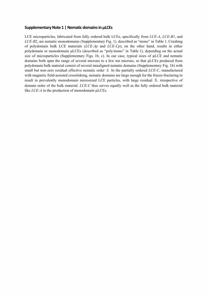
is obtained that results in (see relation (2))

2 2 2 2

3/22

e 1 1 2e 3e arctan e 1.

2 e 1

t t t t

tQ t

(13)

Alignment timescale. The resulting ( )Q t increases monotonously in time, with limiting values

( 0) 0Q t for initial isotropic distribution at 0t and ( ) 1Q t for fully aligned LCE

microparticles at t (Supplementary Fig. 2). By choosing 0.9Q as a criterion for satisfactory

alignment, the respective alignment time is estimated as 0 ( 0.9) 3.1 .t Q Taking into account

relation (6), we finally derive

0 2,

S B

018.

(14)

With the above listed values of , , and S we obtain 3 2/ 1.3 ,10 s TS specifically

0 ( )1T 22 minB and 0 9 T( ) 17 s.B

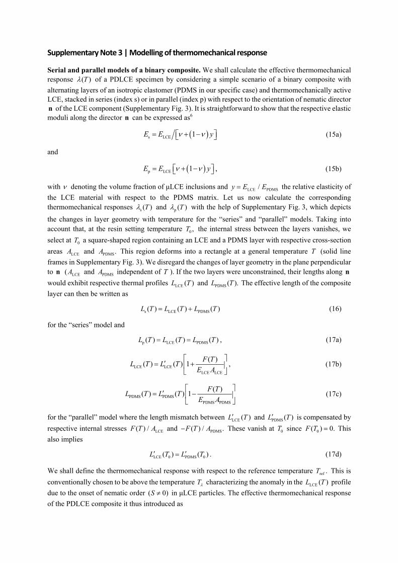
Supplementary Note 3 | Modelling of thermomechanical response 

Serial and parallel models of a binary composite. We shall calculate the effective thermomechanical response ( )T of a PDLCE specimen by considering a simple scenario of a binary composite with

alternating layers of an isotropic elastomer (PDMS in our specific case) and thermomechanically active LCE, stacked in series (index s) or in parallel (index p) with respect to the orientation of nematic director n of the LCE component (Supplementary Fig. 3). It is straightforward to show that the respective elastic moduli along the director n can be expressed as6

s LCE 1 E E y (15a)

and

p LCE 1 , E E y (15b)

with denoting the volume fraction of μLCE inclusions and LCE PDMS/y E E the relative elasticity of

the LCE material with respect to the PDMS matrix. Let us now calculate the corresponding thermomechanical responses s ( ) T and p ( ) T with the help of Supplementary Fig. 3, which depicts

the changes in layer geometry with temperature for the “series” and “parallel” models. Taking into account that, at the resin setting temperature 0 ,T the internal stress between the layers vanishes, we

select at 0T a square-shaped region containing an LCE and a PDMS layer with respective cross-section

areas LCEA and PDMS.A This region deforms into a rectangle at a general temperature T (solid line

frames in Supplementary Fig. 3). We disregard the changes of layer geometry in the plane perpendicular to n LCE(A and PDMSA independent of T ). If the two layers were unconstrained, their lengths along n

would exhibit respective thermal profiles LCE ( )L T and PDMS ( ).L T The effective length of the composite

layer can then be written as

s LCE PDMS( ) ( ) ( ) L T L T L T (16)

for the “series” model and

p LCE PDMS( ) ( ) ( ) , L T L T L T (17a)

LCE LCELCE LCE

( )( ) ( ) 1 ,

F TL T L T

E A

(17b)

PDMS PDMSPDMS PDMS

( )( ) ( ) 1

F TL T L T

E A

(17c)

for the “parallel” model where the length mismatch between LCE ( )L T and PDMS ( )L T is compensated by

respective internal stresses LCE( ) /F T A and PDMS( ) / .F T A These vanish at 0T since 0( ) 0.F T This

also implies

LCE 0 PDMS 0( ) ( ) .L T L T (17d)

We shall define the thermomechanical response with respect to the reference temperature ref .T This is

conventionally chosen to be above the temperature T characterizing the anomaly in the LCE ( )L T profile

due to the onset of nematic order ( 0)S in μLCE particles. The effective thermomechanical response

of the PDLCE composite it thus introduced as

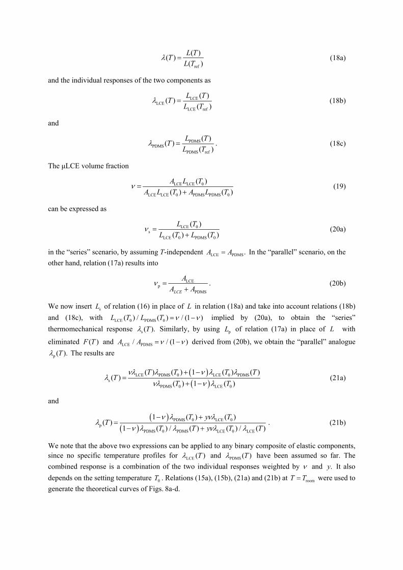
ref

( )( )

( )

L TT

L T (18a)

and the individual responses of the two components as

LCELCE

LCE ref

( )( )

( )

L TT

L T (18b)

and

PDMSPDMS

PDMS ref

( )( ) .

( )

L TT

L T (18c)

The μLCE volume fraction

LCE LCE 0

LCE LCE 0 PDMS PDMS 0

( )

( ) ( )

A L T

A L T A L T

(19)

can be expressed as

LCE 0s

LCE 0 PDMS 0

( )

( ) ( )

L T

L T L T (20a)

in the “series” scenario, by assuming T-independent LCE PDMS.A A In the “parallel” scenario, on the

other hand, relation (17a) results into

LCEp

PDMS

. LCE

A

A A (20b)

We now insert sL of relation (16) in place of L in relation (18a) and take into account relations (18b)

and (18c), with LCE 0 PDMS 0( ) / ( ) / (1 )L T L T implied by (20a), to obtain the “series”

thermomechanical response s ( ). T Similarly, by using pL of relation (17a) in place of L with

eliminated ( )F T and LCE PDMS/ / (1 )A A derived from (20b), we obtain the “parallel” analogue

p ( ). T The results are

LCE PDMS 0 LCE 0 PDMSs

PDMS 0 LCE 0

( ) ( ) 1 ( ) ( )( )

( ) 1 ( )

T T T TT

T T (21a)

and

PDMS 0 LCE 0

pPDMS 0 PDMS LCE 0 LCE

1 ( ) ( )( ) .

1 ( ) / ( ) ( ) / ( )

T y TT

T T y T T (21b)

We note that the above two expressions can be applied to any binary composite of elastic components, since no specific temperature profiles for LCE ( )T and PDMS ( )T have been assumed so far. The

combined response is a combination of the two individual responses weighted by and .y It also

depends on the setting temperature 0T . Relations (15a), (15b), (21a) and (21b) at roomT T were used to

generate the theoretical curves of Figs. 8a-d.

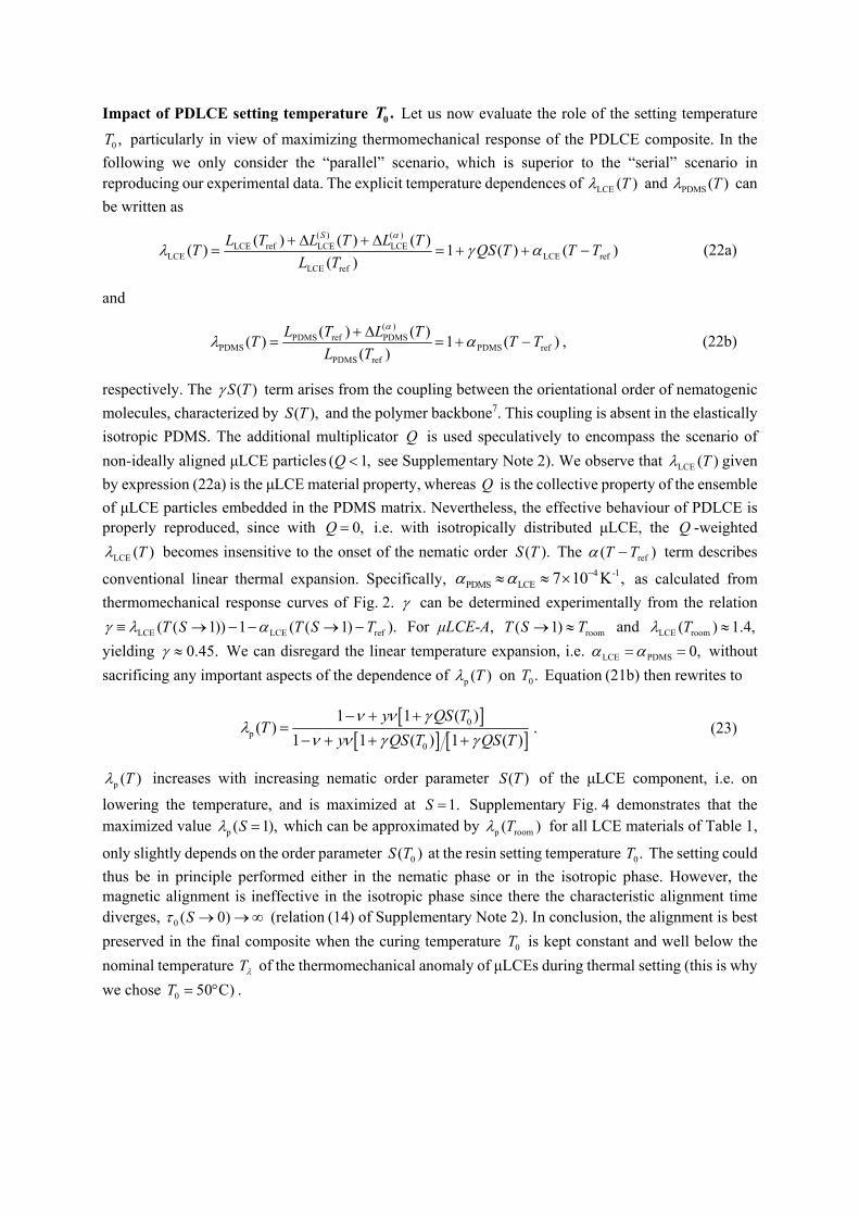
Impact of PDLCE setting temperature 0 .T Let us now evaluate the role of the setting temperature

0 ,T particularly in view of maximizing thermomechanical response of the PDLCE composite. In the

following we only consider the “parallel” scenario, which is superior to the “serial” scenario in reproducing our experimental data. The explicit temperature dependences of LCE ( )T and PDMS ( )T can

be written as

LCE ref LCE LCELCE LCE ref

LCE re

) ( )

f

(( ) ( ) ( )( ) 1 ( ) ( )

( )

SL T L T L TT

L TQS T T T

(22a)

and

PDMS ref PDMSPDMS PDMS ref

(

PDMS re

)

f

( ) ( )( ) 1 ( ) ,

( )

L T L TT T T

L T

(22b)

respectively. The ( )S T term arises from the coupling between the orientational order of nematogenic

molecules, characterized by ( ),S T and the polymer backbone7. This coupling is absent in the elastically

isotropic PDMS. The additional multiplicator Q is used speculatively to encompass the scenario of

non-ideally aligned μLCE particles ( 1,Q see Supplementary Note 2). We observe that LCE ( )T given

by expression (22a) is the μLCE material property, whereas Q is the collective property of the ensemble

of μLCE particles embedded in the PDMS matrix. Nevertheless, the effective behaviour of PDLCE is properly reproduced, since with 0,Q i.e. with isotropically distributed μLCE, the Q -weighted

LCE ( )T becomes insensitive to the onset of the nematic order ( ).S T The ref( )T T term describes

conventional linear thermal expansion. Specifically, 4 -1PDMS LCE 7 10 ,K as calculated from

thermomechanical response curves of Fig. 2. can be determined experimentally from the relation

LCE LCE ref( ( 1)) 1 ( ( 1) ).T S T S T For μLCE-A, room( 1)T S T and LCE room( ) 1.4,T

yielding 0.45. We can disregard the linear temperature expansion, i.e. LCE PDMS 0, without

sacrificing any important aspects of the dependence of p ( ) T on 0.T Equation (21b) then rewrites to

0

p0

1 1 ( )( )

1 1 ( ) 1 ( ).

Q

Q Q

y S TT

y S T S T (23)

p ( ) T increases with increasing nematic order parameter ( )S T of the μLCE component, i.e. on

lowering the temperature, and is maximized at 1.S Supplementary Fig. 4 demonstrates that the maximized value p ( 1), S which can be approximated by p room( ) T for all LCE materials of Table 1,

only slightly depends on the order parameter 0( )S T at the resin setting temperature 0.T The setting could

thus be in principle performed either in the nematic phase or in the isotropic phase. However, the magnetic alignment is ineffective in the isotropic phase since there the characteristic alignment time diverges, 0 ( 0)S (relation (14) of Supplementary Note 2). In conclusion, the alignment is best

preserved in the final composite when the curing temperature 0T is kept constant and well below the

nominal temperature T of the thermomechanical anomaly of μLCEs during thermal setting (this is why

we chose 0 50 C)T .

Supplementary References 

1. Lebar, A., Kutnjak, Z., Žumer, S., Finkelmann, H., Sánchez-Ferrer A. & Zalar, B. Evidence of supercritical behaviour in liquid single crystal elastomers. Phys. Rev. Lett. 94, 197801 (2005).

2. Doi, M. & Edwards, S. F. Theory of Polymer Dynamics (Clarendon Press, Oxford, 1986). 3. Milavec, J., Domenici, V., Zupančič, B., Rešetič, A., Bubnov, A. & Zalar, B. Deuteron NMR resolved mesogen vs. crosslinker molecular

order and reorientational exchange in liquid single crystal elastomers. Phys. Chem. Chem. Phys. 18, 4071-4077 (2016). 4. Schad, Hp., Baur, G. & Meier, G. Investigation of the dielectric constants and the diamagnetic anisotropies of cyanobiphenyls (CB),

cyanophenylcyclohexanes (PCH), and cyanocyclohexylcyclohexanes (CCH) in the nematic phase. J. Chem. Phys. 71, 3147-3181 (1979). 5. Kimura, T., Yamato, M., Koshimizu, W., Koike, M. & Kawai, T. Magnetic orientation of polymer fibers in suspension. Langmuir 16,

858-861 (2000). 6. Daniel, I. & Ishai, O. Engineering Mechanics of Composite Materials (Oxford Univ. Press, 2007). 7. Warner, M. & Terentjev, E. M. Liquid Crystal Elastomers (Oxford Univ. Press, 2007).