Path-loss and Shadowing(Large-scale Fading)

PROF. MICHAEL TSAI

2014/03/23

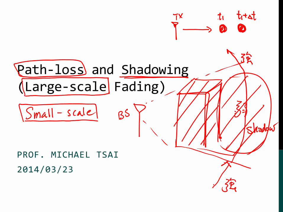
Friis Formula

TX Antenna

EIRP=𝑃𝑡𝐺𝑡

𝑑

Power spatial density𝑊

𝑚2

1

4𝜋𝑑2

𝐴𝑒

×

×

RX Antenna

⇒ 𝑃𝑟=𝑃𝑡𝐺𝑡𝐴𝑒4𝜋𝑑2

2

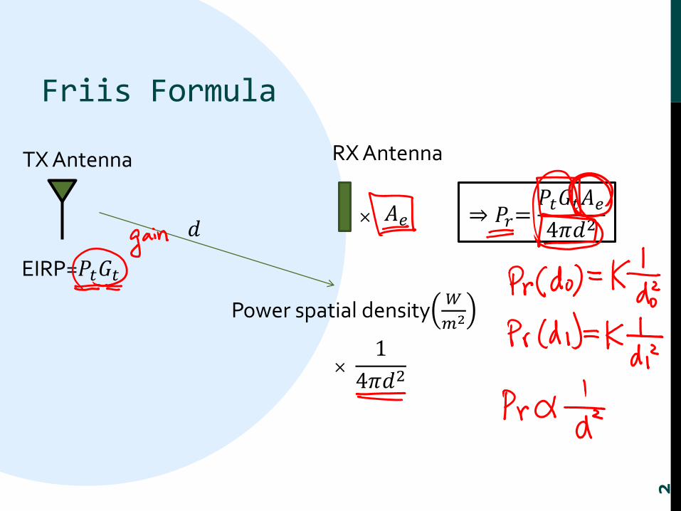
Antenna Aperture

• Antenna Aperture=Effective Area

• Isotropic Antenna’s effective area 𝑨𝒆,𝒊𝒔𝒐 ≐𝝀𝟐

𝟒𝝅

• Isotropic Antenna’s Gain=1

• 𝑮 =𝟒𝝅

𝝀𝟐𝑨𝒆

• Friis Formula becomes: 𝑷𝒓 =𝑷𝒕𝑮𝒕𝑮𝒓𝝀

𝟐

𝟒𝝅𝒅 𝟐 =𝑷𝒕𝑨𝒕𝑨𝒓

𝝀𝟐𝒅𝟐

3

𝑷𝒓 =𝑷𝒕𝑮𝒕𝐴𝑒4𝜋𝑑2

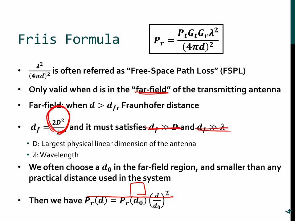
Friis Formula

•𝝀𝟐

𝟒𝝅𝒅 𝟐 is often referred as “Free-Space Path Loss” (FSPL)

• Only valid when d is in the “far-field” of the transmitting antenna

• Far-field: when 𝒅 > 𝒅𝒇, Fraunhofer distance

• 𝒅𝒇 =𝟐𝑫𝟐

𝝀, and it must satisfies 𝒅𝒇 ≫ 𝑫 and 𝒅𝒇 ≫ 𝝀

• D: Largest physical linear dimension of the antenna

• 𝜆: Wavelength

• We often choose a 𝒅𝟎 in the far-field region, and smaller than any practical distance used in the system

• Then we have 𝑷𝒓 𝒅 = 𝑷𝒓 𝒅𝟎𝒅

𝒅𝟎

𝟐

𝑷𝒓 =𝑷𝒕𝑮𝒕𝑮𝒓𝝀

𝟐

𝟒𝝅𝒅 𝟐

4

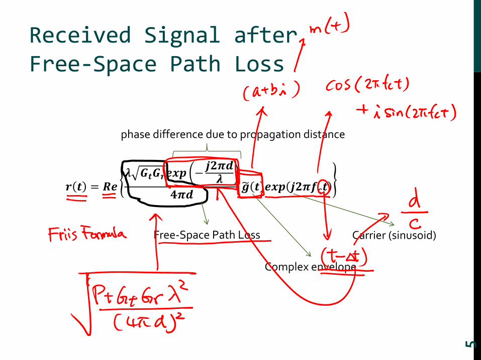
Received Signal after Free-Space Path Loss

𝒓 𝒕 = 𝑹𝒆𝝀 𝑮𝒕𝑮𝒓𝒆𝒙𝒑 −

𝒋𝟐𝝅𝒅𝝀

𝟒𝝅𝒅 𝒈 𝒕 𝒆𝒙𝒑 𝒋𝟐𝝅𝒇𝒄𝒕

phase difference due to propagation distance

Free-Space Path Loss

Complex envelope

Carrier (sinusoid)

5

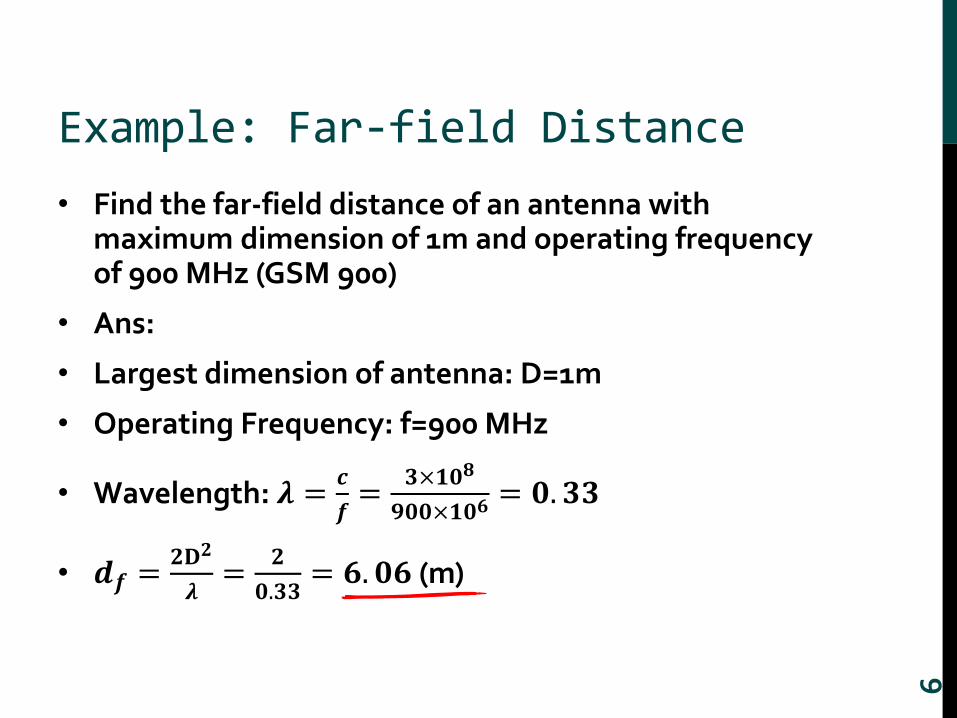
Example: Far-field Distance

• Find the far-field distance of an antenna with maximum dimension of 1m and operating frequency of 900 MHz (GSM 900)

• Ans:

• Largest dimension of antenna: D=1m

• Operating Frequency: f=900 MHz

• Wavelength: 𝝀 =𝒄

𝒇=

𝟑×𝟏𝟎𝟖

𝟗𝟎𝟎×𝟏𝟎𝟔= 𝟎. 𝟑𝟑

• 𝒅𝒇 =𝟐𝐃𝟐

𝝀=

𝟐

𝟎.𝟑𝟑= 𝟔. 𝟎𝟔 (m)

6

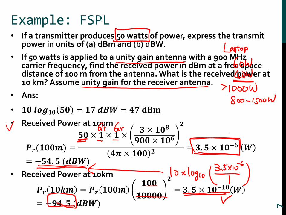
Example: FSPL • If a transmitter produces 50 watts of power, express the transmit

power in units of (a) dBm and (b) dBW.

• If 50 watts is applied to a unity gain antenna with a 900 MHz carrier frequency, find the received power in dBm at a free space distance of 100 m from the antenna. What is the received power at 10 km? Assume unity gain for the receiver antenna.

• Ans:

• 𝟏𝟎 𝒍𝒐𝒈𝟏𝟎 𝟓𝟎 = 𝟏𝟕 𝒅𝑩𝑾 = 𝟒𝟕 𝐝𝐁𝐦

• Received Power at 100m

𝑷𝒓(𝟏𝟎𝟎𝒎) =

𝟓𝟎 × 𝟏 × 𝟏 ×𝟑 × 𝟏𝟎𝟖

𝟗𝟎𝟎 × 𝟏𝟎𝟔

𝟐

𝟒𝝅 × 𝟏𝟎𝟎 𝟐 = 𝟑. 𝟓 × 𝟏𝟎−𝟔 𝑾

= −𝟓𝟒. 𝟓 (𝒅𝑩𝑾)

• Received Power at 10km

𝑷𝒓 𝟏𝟎𝒌𝒎 = 𝑷𝒓 𝟏𝟎𝟎𝒎𝟏𝟎𝟎

𝟏𝟎𝟎𝟎𝟎

𝟐

= 𝟑. 𝟓 × 𝟏𝟎−𝟏𝟎 𝑾

= −𝟗𝟒. 𝟓 (𝒅𝑩𝑾) 7

Two-ray Model

TX Antenna

𝑑

𝜃

𝑙

𝑥 𝑥′

RX Antenna

ℎ𝑡ℎ𝑟

𝐺𝑎

𝐺𝑐𝐺𝑏

𝐺𝑑

𝑟2−𝑟𝑎𝑦 𝑡 =

𝑅𝑒𝜆

4𝜋

𝐺𝑎𝐺𝑏 𝑔 𝑡 exp −𝑗2𝜋𝑙𝜆

𝑙+𝑅 𝐺𝑐𝐺𝑑 𝑔 𝑡 − 𝜏 exp −

𝑗2𝜋 𝑥 + 𝑥′

𝜆

𝑥 + 𝑥′exp 𝑗2𝜋𝑓𝑐𝑡

Delayed since x+x’ is longer. 𝜏 = (𝑥 + 𝑥′ − 𝑙)/𝑐

R: ground reflection coefficient (phase and amplitude change) 8

Two-ray Model: Received Power

• 𝑷𝒓 = 𝑷𝒕𝝀

𝟒𝝅

𝟐 𝑮𝒂𝑮𝒃

𝒍+

𝑮𝒄𝑮𝒅𝒆𝒙𝒑 −𝒋𝚫𝝓

𝒙+𝒙′

𝟐

• The above is verified by empirical results.

• 𝚫𝝓 = 𝟐𝝅(𝒙 + 𝒙′ − 𝒍)/𝝀

• 𝒙 + 𝒙′ − 𝒍 = 𝒉𝒕 + 𝒉𝒓𝟐 + 𝒅𝟐 − 𝒉𝒕 − 𝒉𝒓

𝟐 + 𝒅𝟐

9

l

x

x’

x’

x

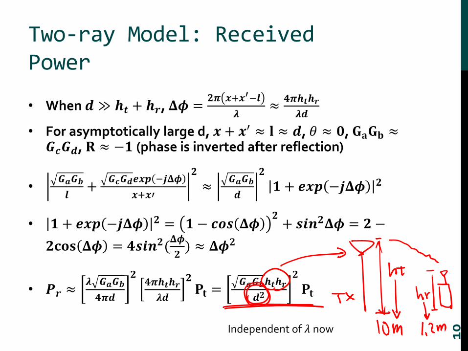
Two-ray Model: Received Power

• When 𝒅 ≫ 𝒉𝒕 + 𝒉𝒓, 𝚫𝝓 =𝟐𝝅 𝒙+𝒙′−𝒍

𝝀≈

𝟒𝝅𝒉𝒕𝒉𝒓

𝝀𝒅

• For asymptotically large d, 𝒙 + 𝒙′ ≈ 𝐥 ≈ 𝒅, 𝜃 ≈ 𝟎, 𝐆𝐚𝐆𝐛 ≈𝑮𝒄𝑮𝒅, 𝐑 ≈ −𝟏 (phase is inverted after reflection)

•𝑮𝒂𝑮𝒃

𝒍+

𝑮𝒄𝑮𝒅𝒆𝒙𝒑 −𝒋𝚫𝝓

𝒙+𝒙′

𝟐

≈𝑮𝒂𝑮𝒃

𝒅

𝟐

𝟏 + 𝒆𝒙𝒑 −𝒋𝚫𝝓 𝟐

• 𝟏 + 𝒆𝒙𝒑 −𝒋𝚫𝝓 𝟐 = 𝟏 − 𝒄𝒐𝒔 𝚫𝝓𝟐+ 𝒔𝒊𝒏𝟐𝚫𝝓 = 𝟐 −

𝟐𝐜𝐨𝐬 𝚫𝝓 = 𝟒𝒔𝒊𝒏𝟐(𝚫𝝓

𝟐) ≈ 𝚫𝝓𝟐

• 𝑷𝒓 ≈𝝀 𝑮𝒂𝑮𝒃

𝟒𝝅𝒅

𝟐𝟒𝝅𝒉𝒕𝒉𝒓

𝝀𝒅

𝟐𝐏𝐭 =

𝑮𝒂𝑮𝒃𝒉𝒕𝒉𝒓

𝒅𝟐

𝟐

𝐏𝐭

10Independent of 𝜆 now

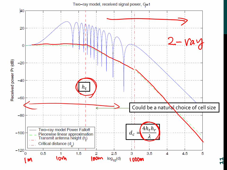
11

𝑑𝑐 =4ℎ𝑡ℎ𝑟𝜆

ℎ𝑡

Could be a natural choice of cell size

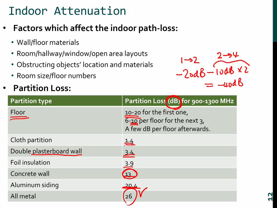
Indoor Attenuation

• Factors which affect the indoor path-loss:

• Wall/floor materials

• Room/hallway/window/open area layouts

• Obstructing objects’ location and materials

• Room size/floor numbers

• Partition Loss:

12

Partition type Partition Loss (dB) for 900-1300 MHz

Floor 10-20 for the first one,6-10 per floor for the next 3,A few dB per floor afterwards.

Cloth partition 1.4

Double plasterboard wall 3.4

Foil insulation 3.9

Concrete wall 13

Aluminum siding 20.4

All metal 26

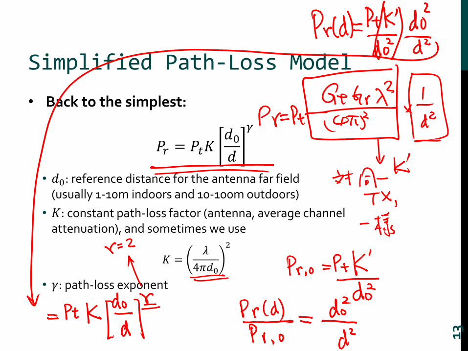
Simplified Path-Loss Model

• Back to the simplest:

• 𝑑0: reference distance for the antenna far field (usually 1-10m indoors and 10-100m outdoors)

• 𝐾: constant path-loss factor (antenna, average channel attenuation), and sometimes we use

• 𝛾: path-loss exponent

13

𝑃𝑟 = 𝑃𝑡𝐾𝑑0𝑑

𝛾

𝐾 =𝜆

4𝜋𝑑0

2

Some empirical results

14

Measurements in Germany Cities

Environment Path-loss Exponent

Free-space 2

Urban area cellular radio 2.7-3.5

Shadowed urban cellular radio

3-5

In building LOS 1.6 to 1.8

Obstructed in building 4 to 6

Obstructed in factories 2 to 3

Empirical Path-Loss Model

• Based on empirical measurements

• over a given distance

• in a given frequency range

• for a particular geographical area or building

• Could be applicable to other environments as well

• Less accurate in a more general environment

• Analytical model: 𝑷𝒓/𝑷𝒕 is characterized as a function of distance.

• Empirical Model: 𝑷𝒓/𝑷𝒕 is a function of distance including the effects of path loss, shadowing, and multipath.

• Need to average the received power measurements to remove multipath effects Local Mean Attenuation (LMA) at distance d.

15

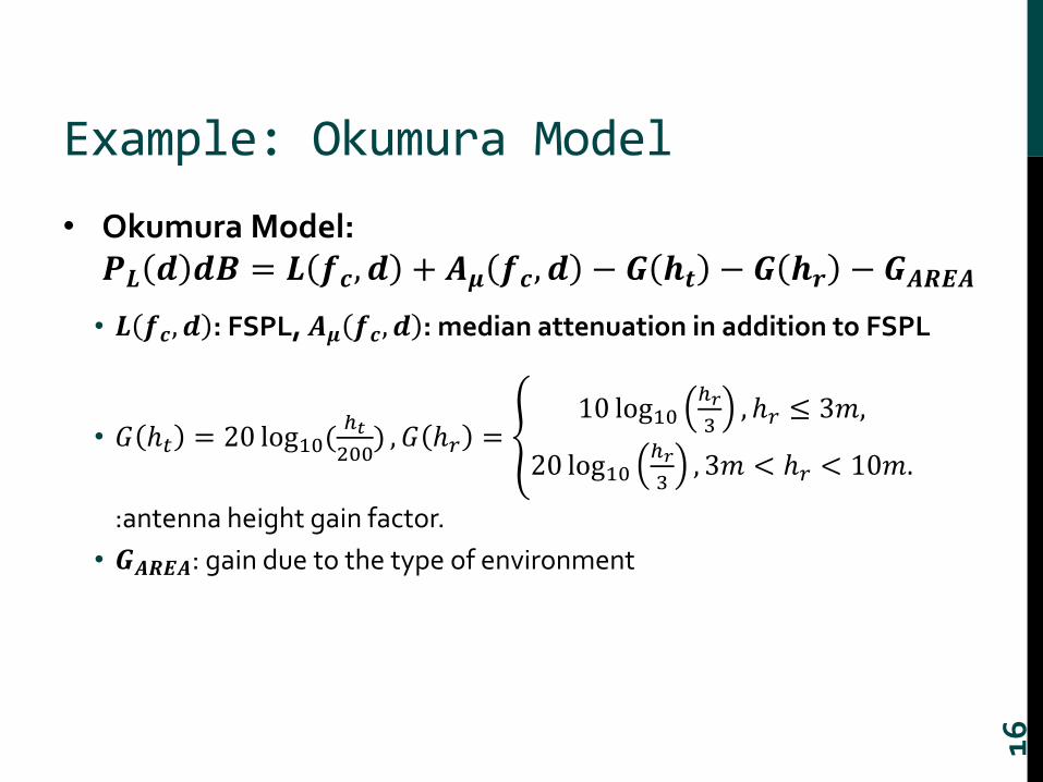
Example: Okumura Model

• Okumura Model:𝑷𝑳 𝒅 𝒅𝑩 = 𝑳 𝒇𝒄, 𝒅 + 𝑨𝝁 𝒇𝒄, 𝒅 − 𝑮 𝒉𝒕 − 𝑮 𝒉𝒓 − 𝑮𝑨𝑹𝑬𝑨

• 𝑳 𝒇𝒄, 𝒅 : FSPL, 𝑨𝝁 𝒇𝒄, 𝒅 : median attenuation in addition to FSPL

• 𝐺 ℎ𝑡 = 20 log10(ℎ𝑡

200) , 𝐺 ℎ𝑟 =

10 log10ℎ𝑟

3, ℎ𝑟 ≤ 3𝑚,

20 log10ℎ𝑟

3, 3𝑚 < ℎ𝑟 < 10𝑚.

:antenna height gain factor.

• 𝑮𝑨𝑹𝑬𝑨: gain due to the type of environment

16

Example: Piecewise Linear Model

• N segments with N-1 “breakpoints”

• Applicable to both outdoor and indoor channels

• Example – dual-slope model:

• 𝐾: constant path-loss factor

• 𝛾1: path-loss exponent for 𝑑0~𝑑𝑐• 𝛾2: path-loss exponent after 𝑑𝑐 17

𝑃𝑟 𝑑 =

𝑃𝑡𝐾𝑑0𝑑

𝛾1

𝑃𝑡𝐾𝑑𝑐𝑑

𝛾1 𝑑

𝑑𝑐

𝛾2

𝑑0 ≤ 𝑑 ≤ 𝑑𝑐 ,

𝑑 > 𝑑𝑐.

Shadow Fading

• Same T-R distance usually have different path loss

• Surrounding environment is different

• Reality: simplified Path-Loss Model represents an “average”

• How to represent the difference between the average and the actual path loss?

• Empirical measurements have shown that

• it is random (and so is a random variable)

• Log-normal distributed

18

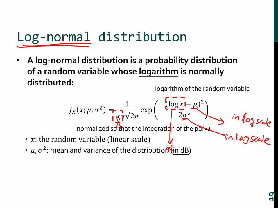
Log-normal distribution

• A log-normal distribution is a probability distribution of a random variable whose logarithm is normally distributed:

• 𝑥: the random variable (linear scale)

• 𝜇, 𝜎2: mean and variance of the distribution (in dB)

19

𝑓𝑋 𝑥; 𝜇, 𝜎2 =1

𝑥𝜎 2𝜋exp −

log 𝑥 − 𝜇 2

2𝜎2

logarithm of the random variable

normalized so that the integration of the pdf=1

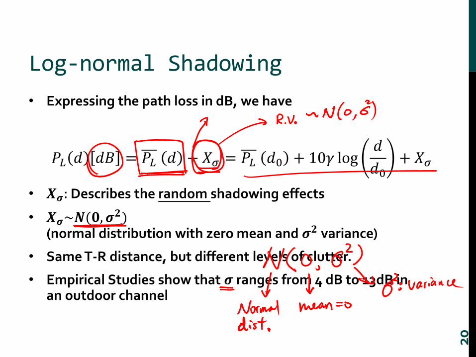
Log-normal Shadowing

• Expressing the path loss in dB, we have

• 𝑿𝝈: Describes the random shadowing effects

• 𝑿𝝈~𝑵(𝟎, 𝝈𝟐)

(normal distribution with zero mean and 𝝈𝟐 variance)

• Same T-R distance, but different levels of clutter.

• Empirical Studies show that 𝝈 ranges from 4 dB to 13dB in an outdoor channel

20

𝑃𝐿 𝑑 𝑑𝐵 = 𝑃𝐿 𝑑 + 𝑋𝜎 = 𝑃𝐿 𝑑0 + 10𝛾 log𝑑

𝑑0+ 𝑋𝜎

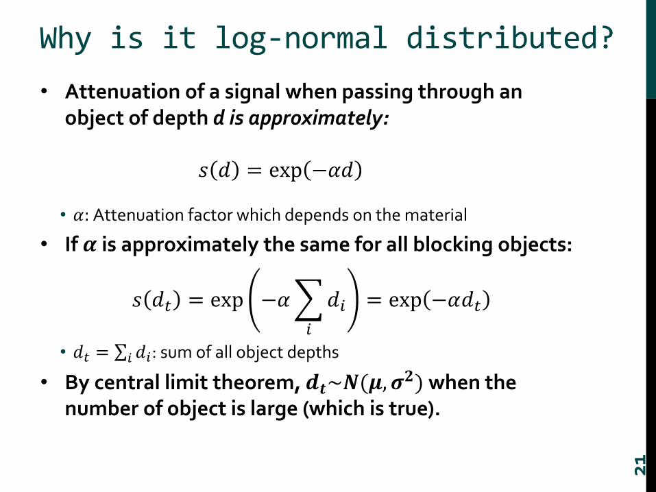
Why is it log-normal distributed?

• Attenuation of a signal when passing through an object of depth d is approximately:

• 𝛼: Attenuation factor which depends on the material

• If 𝜶 is approximately the same for all blocking objects:

• 𝑑𝑡 = 𝑖 𝑑𝑖: sum of all object depths

• By central limit theorem, 𝒅𝒕~𝑵(𝝁, 𝝈𝟐) when the

number of object is large (which is true).

21

𝑠 𝑑 = exp −𝛼𝑑

𝑠 𝑑𝑡 = exp −𝛼

𝑖

𝑑𝑖 = exp −𝛼𝑑𝑡

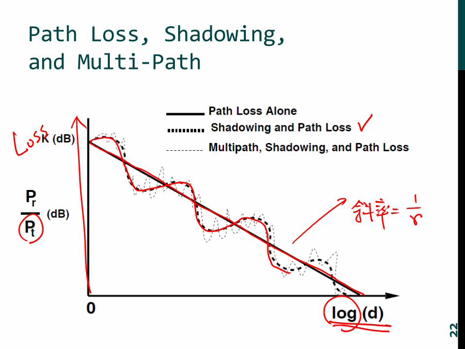
Path Loss, Shadowing, and Multi-Path

22

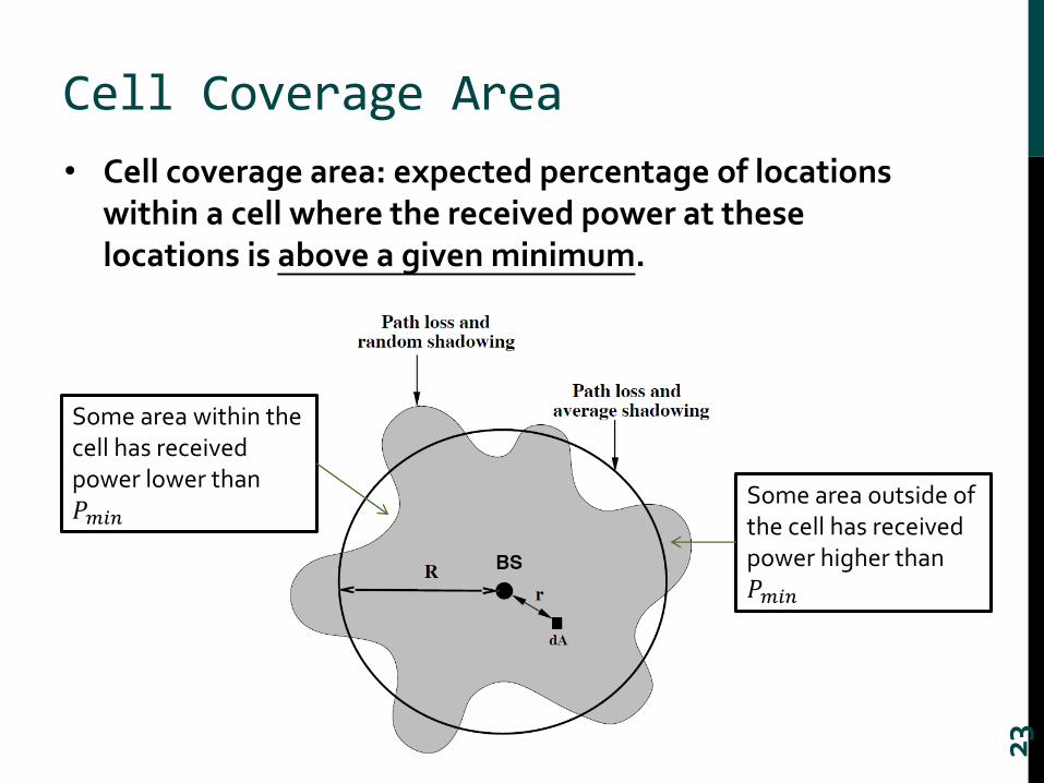
Cell Coverage Area

• Cell coverage area: expected percentage of locations within a cell where the received power at these locations is above a given minimum.

23

Some area within the cell has received power lower than 𝑃𝑚𝑖𝑛

Some area outside of the cell has received power higher than 𝑃𝑚𝑖𝑛

Cell Coverage Area

• We can boost the transmission power at the BS

• Extra interference to the neighbor cells

• In fact, any mobile in the cell has a nonzero probability of having its received power below 𝑷𝒎𝒊𝒏.

• Since Normal distribution has infinite tails

• Make sense in the real-world: in a tunnel, blocked by large buildings, doesn’t matter if it is very close to the BS

24

Cell Coverage Area

• Cell coverage area is given by

• 𝑷𝑨 ≐ 𝒑 𝑷𝒓 𝒓 > 𝑷𝒎𝒊𝒏

25

𝑪 = 𝑬𝟏

𝝅𝑹𝟐 𝒄𝒆𝒍𝒍 𝒂𝒓𝒆𝒂

𝟏 𝑷𝒓 𝒓 > 𝑷𝒎𝒊𝒏 𝒊𝒏 𝒅𝑨 𝒅𝑨

=𝟏

𝝅𝑹𝟐 𝒄𝒆𝒍𝒍 𝒂𝒓𝒆𝒂

𝑬 𝟏 𝑷𝒓 𝒓 > 𝑷𝒎𝒊𝒏 𝒊𝒏 𝒅𝑨 𝒅𝑨

1 if the statement is true, 0 otherwise. (indicator function)

𝑪 =𝟏

𝝅𝑹𝟐 𝒄𝒆𝒍𝒍 𝒂𝒓𝒆𝒂

𝑷𝑨𝒅𝑨 =𝟏

𝝅𝑹𝟐 𝟎

𝟐𝝅

𝟎

𝑹

𝑷𝑨 𝒓𝒅𝒓 𝒅𝜽

Cell Coverage Area

• Q-function:

26

𝑃𝐴 = 𝑝 𝑃𝑟 𝑟 ≥ 𝑃𝑚𝑖𝑛 = 𝑄𝑃𝑚𝑖𝑛 − 𝑃𝑡 − 𝑃𝐿 𝑟

𝜎

𝑄 𝑧 ≐ 𝑝 𝑋 > 𝑧 = 𝑧

∞ 1

2𝜋exp −

𝑦2

2𝑑𝑦

Log-normal distribution’s standard deviation

z

Cell Coverage Area

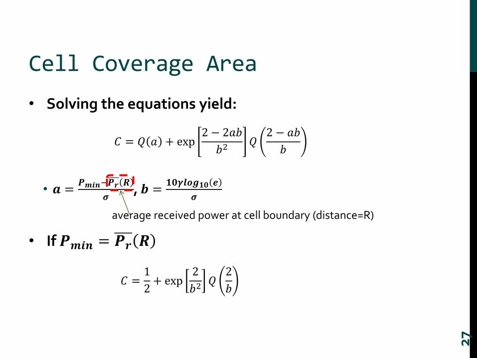
• Solving the equations yield:

• 𝒂 =𝑷𝒎𝒊𝒏−𝑷𝒓 𝑹

𝝈, 𝒃 =

𝟏𝟎𝜸𝒍𝒐𝒈𝟏𝟎 𝒆

𝝈

• If 𝑷𝒎𝒊𝒏 = 𝑷𝒓 𝑹

27

𝐶 = 𝑄 𝑎 + exp2 − 2𝑎𝑏

𝑏2𝑄

2 − 𝑎𝑏

𝑏

average received power at cell boundary (distance=R)

𝐶 =1

2+ exp

2

𝑏2𝑄

2

𝑏

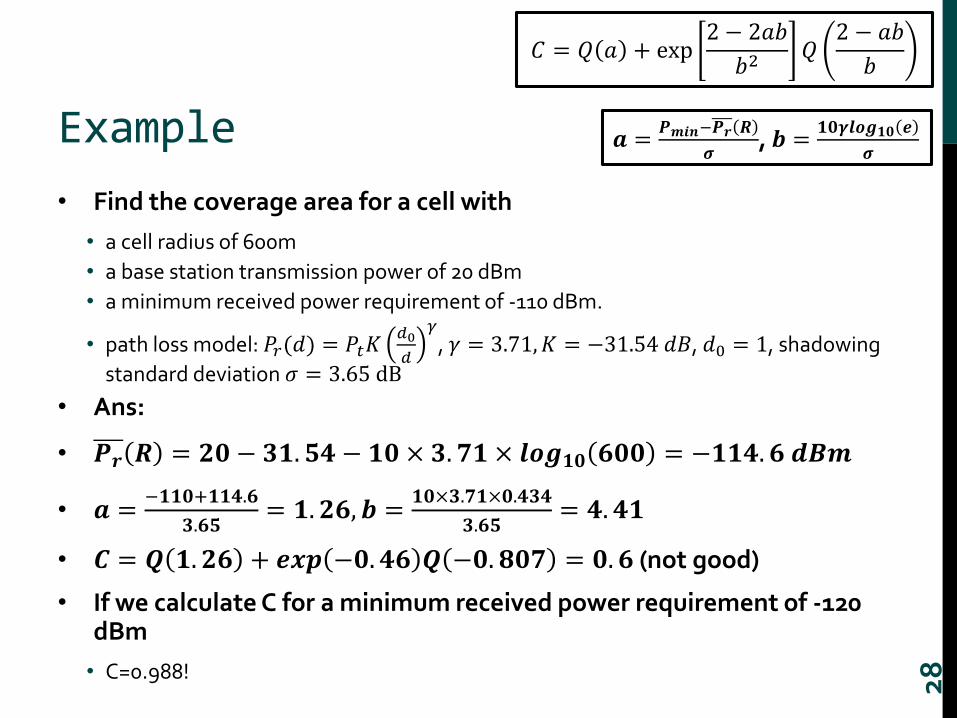
Example

• Find the coverage area for a cell with

• a cell radius of 600m

• a base station transmission power of 20 dBm

• a minimum received power requirement of -110 dBm.

• path loss model: 𝑃𝑟(𝑑) = 𝑃𝑡𝐾𝑑0

𝑑

𝛾, 𝛾 = 3.71,𝐾 = −31.54 𝑑𝐵, 𝑑0 = 1, shadowing

standard deviation 𝜎 = 3.65 dB

• Ans:

• 𝑷𝒓 𝑹 = 𝟐𝟎 − 𝟑𝟏. 𝟓𝟒 − 𝟏𝟎 × 𝟑. 𝟕𝟏 × 𝒍𝒐𝒈𝟏𝟎 𝟔𝟎𝟎 = −𝟏𝟏𝟒. 𝟔 𝒅𝑩𝒎

• 𝒂 =−𝟏𝟏𝟎+𝟏𝟏𝟒.𝟔

𝟑.𝟔𝟓= 𝟏. 𝟐𝟔, 𝒃 =

𝟏𝟎×𝟑.𝟕𝟏×𝟎.𝟒𝟑𝟒

𝟑.𝟔𝟓= 𝟒. 𝟒𝟏

• 𝑪 = 𝑸 𝟏. 𝟐𝟔 + 𝒆𝒙𝒑 −𝟎. 𝟒𝟔 𝑸 −𝟎. 𝟖𝟎𝟕 = 𝟎. 𝟔 (not good)

• If we calculate C for a minimum received power requirement of -120 dBm

• C=0.988!

28

𝐶 = 𝑄 𝑎 + exp2 − 2𝑎𝑏

𝑏2𝑄

2 − 𝑎𝑏

𝑏

𝒂 =𝑷𝒎𝒊𝒏−𝑷𝒓 𝑹

𝝈, 𝒃 =

𝟏𝟎𝜸𝒍𝒐𝒈𝟏𝟎 𝒆

𝝈

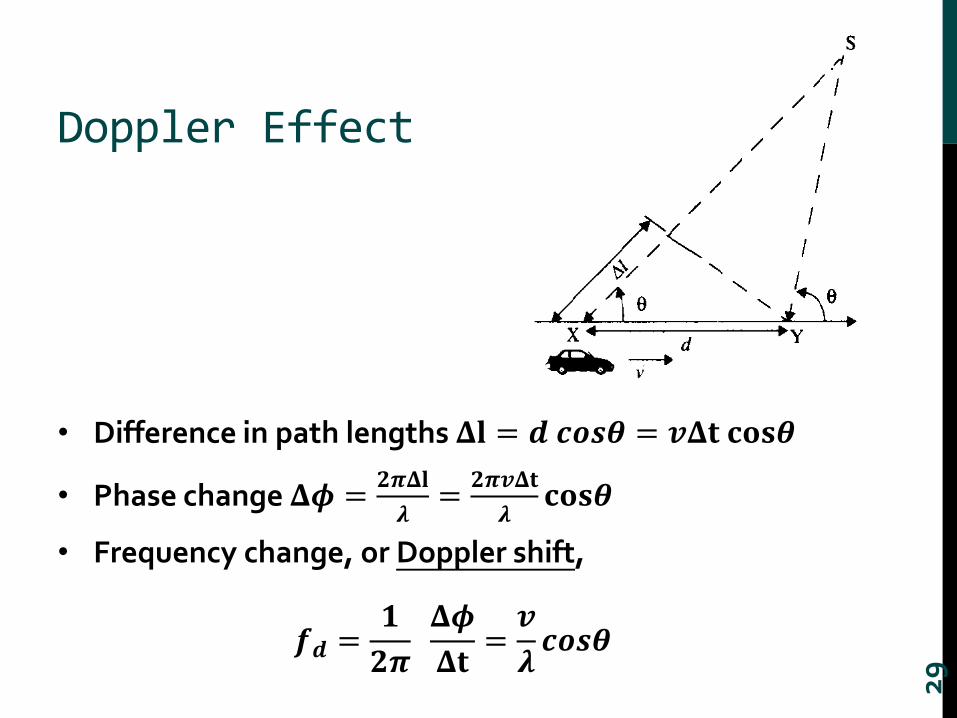
Doppler Effect

• Difference in path lengths 𝚫𝐥 = 𝒅 𝒄𝒐𝒔𝜽 = 𝒗𝚫𝐭 𝐜𝐨𝐬𝜽

• Phase change 𝚫𝝓 =𝟐𝝅𝚫𝐥

𝝀=

𝟐𝝅𝒗𝚫𝐭

𝝀𝐜𝐨𝐬𝜽

• Frequency change, or Doppler shift,

𝒇𝒅 =𝟏

𝟐𝝅

𝚫𝝓

𝚫𝐭=𝒗

𝝀𝒄𝒐𝒔𝜽

29

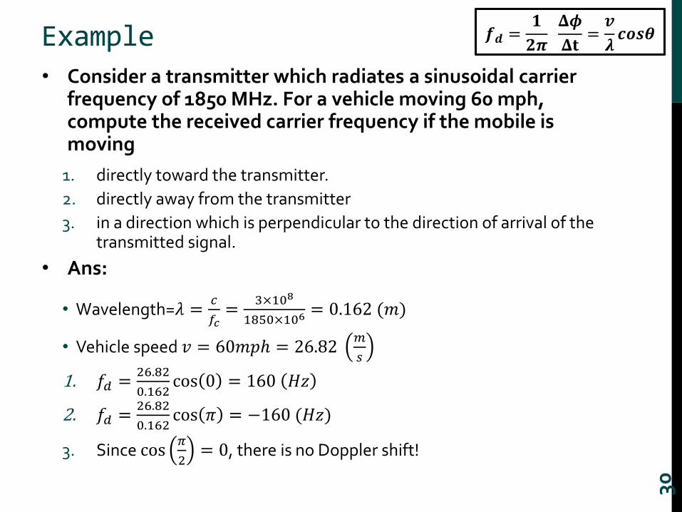
Example• Consider a transmitter which radiates a sinusoidal carrier

frequency of 1850 MHz. For a vehicle moving 60 mph, compute the received carrier frequency if the mobile is moving

1. directly toward the transmitter.

2. directly away from the transmitter

3. in a direction which is perpendicular to the direction of arrival of the transmitted signal.

• Ans:

• Wavelength=𝜆 =𝑐

𝑓𝑐=

3×108

1850×106= 0.162 (𝑚)

• Vehicle speed 𝑣 = 60𝑚𝑝ℎ = 26.82𝑚

𝑠

1. 𝑓𝑑 =26.82

0.162cos 0 = 160 𝐻𝑧

2. 𝑓𝑑 =26.82

0.162cos 𝜋 = −160 (𝐻𝑧)

3. Since cos𝜋

2= 0, there is no Doppler shift!

30

𝒇𝒅 =𝟏

𝟐𝝅

𝚫𝝓

𝚫𝐭=𝒗

𝝀𝒄𝒐𝒔𝜽

Doppler Effect

• If the car (mobile) is moving toward the direction of the arriving wave, the Doppler shift is positive

• Different Doppler shifts if different 𝜽 (incoming angle)

• Multi-path: all different angles

• Many Doppler shifts Doppler spread

31