Embed Size (px)
Citation preview

PPaasstt aanndd PPrroojjeecctteedd TTrreennddss iinn CClliimmaattee aanndd SSeeaa LLeevveell ffoorr SSoouutthh FFlloorriiddaa
HHyyddrroollooggiicc aanndd EEnnvviirroonnmmeennttaall SSyysstteemmss MMooddeelliinngg
TTeecchhnniiccaall RReeppoorrtt
JJuullyy 22001111
Photo courtesy of National Aeronautics and Space Administration

PAST AND PROJECTED TRENDS IN CLIMATE AND SEA LEVEL FOR
SOUTH FLORIDA
July 5, 2011
Team Members:
J. Obeysekera J. Park
M. Irizarry-Ortiz P. Trimble J. Barnes
J. VanArman W. Said
E. Gadzinski
Hydrologic and Environmental Systems Modeling South Florida Water Management District
3301 Gun Club Road
West Palm Beach, Florida


Contents
iii Technical Report July 5, 2011
PAST AND PROJECTED TRENDS IN CLIMATE AND SEA LEVEL FOR SOUTH FLORIDA
Table of Contents
List of Figures ........................................................................................................... v
List of Tables ............................................................................................................ x
Acknowledgments ................................................................................................. xii
Recommended Citation ....................................................................................... xiii
List of Acronyms and Abbreviations ................................................................. xiv
Executive Summary ............................................................................................ xvii
PAST AND PROJECTED TRENDS IN CLIMATE AND SEA LEVEL FOR SOUTH FLORIDA ........................................................................................ 1
I. Introduction .................................................................................................... 1
II. Modes of Natural Variability that Influence Florida’s Climate ............... 5
El Niño Southern Oscillation ...................................................................................................... 6
Pacific Decadal Oscillation ......................................................................................................... 9
Atlantic Multi-decadal Oscillation ............................................................................................ 12
North Atlantic Oscillation ......................................................................................................... 14
Variations of Solar Activity ...................................................................................................... 15
III. Historical Trends in Florida Temperature and Precipitation .................... 19
Introduction ............................................................................................................................... 19
Previous Studies ........................................................................................................................ 20
Temperature Trends .............................................................................................................. 20
Precipitation Trends .............................................................................................................. 22

Trends in Climate and Sea Level Rise for South Florida
iv Technical Report July 5, 2011
Data ........................................................................................................................................... 23
Methods..................................................................................................................................... 26
Mann-Kendall Trend Test and Sen-Theil Regression .......................................................... 26
Trends in Extremes Based on the GEV Distribution ............................................................ 29
Results and Discussion ............................................................................................................. 30
Precipitation .......................................................................................................................... 36
Temperature .......................................................................................................................... 39
Conclusions ............................................................................................................................... 52
IV. Climate Projections ......................................................................................... 55
Introduction ............................................................................................................................... 55
General Circulation Models ...................................................................................................... 55
Precipitation .......................................................................................................................... 58
Temperature .......................................................................................................................... 61
GCM projections ................................................................................................................... 63
Regional Climate Models ......................................................................................................... 66
Validation of Statistically Downscaled Climate Data .......................................................... 66
Projections of Statistically Downscaled Data ....................................................................... 71
Dynamically Downscaled Climate Data ................................................................................... 79
Data and Methods ................................................................................................................. 80
NARCCAP Model Validation and Projections ..................................................................... 82
Projections............................................................................................................................. 90
Summary ................................................................................................................................... 91
V. Sea Level Rise and Extremes ...................................................................... 93
Introduction ............................................................................................................................... 93
Sea Level Rise Components ..................................................................................................... 94
Historic Sea Level and Projections ........................................................................................... 95
IPCC Projections ................................................................................................................... 96
Government and Working Group Projections ...................................................................... 97
Recent Scientific Literature Projections ............................................................................... 99
Contents
v Technical Report July 5, 2011
Extreme Events in South Florida ............................................................................................ 100
Climate Links to Extreme Events ........................................................................................... 102
AMO Relation to Florida Storm Surge ............................................................................... 102
Analysis............................................................................................................................... 109
Projection of Extreme Events ................................................................................................. 109
Historical Storm Surge Distributions .................................................................................. 110
Surge Projections ................................................................................................................ 112
Analysis............................................................................................................................... 117
Coastal Structure Vulnerability ............................................................................................... 117
Saltwater Intrusion Vulnerability ............................................................................................ 121
Decision Support ..................................................................................................................... 121
Economics ............................................................................................................................... 122
Conclusion – Sea Level Rise .................................................................................................. 123
VI. Water Resources Management Impacts ..................................................127
Simulated Response to Precipitation and Temperature Changes ........................................... 127
Simulated Response to Sea Level Rise ................................................................................... 131
VII. Conclusions and Recommendations ........................................................133
Natural Variability .................................................................................................................. 133
Temperature and Precipitation ................................................................................................ 134
Climate Projections ................................................................................................................. 134
Sea Level Rise ......................................................................................................................... 135
Water Resources Impacts ........................................................................................................ 135
Literature Cited ....................................................................................................137
List of Figures Figure 1. Anticipated Water Management Impacts of Climate Change. ....................................... 2
Figure 2. El Niño-Southern Oscillation (ENSO) ........................................................................... 7
F igure 3. El Niño-Southern Oscillation Niño Regions, Source: NWS, Southern Region Headquarters ..................................................................................................................... 8

Trends in Climate and Sea Level Rise for South Florida
vi Technical Report July 5, 2011
Figure 4. Oceanic Niño Index (ONI), Source: NOAA Climate Services ...................................... 8
Figure 5. Typical Winter weather patterns during La Niña and El Niño Episodes ....................... 9
Figure 6. Comparison of the Pacific Decadal Oscillation Warm phase and El Niño. The spatial pattern of anomalies in sea surface temperature (shading, degrees Celsius) and sea level pressure (contours) associated with the warm phase of PDO for the period 1900-1992. Contour interval is 1 mb, with additional contours drawn for +0.25 and 0.5 mb. Positive (negative) contours are dashed (solid). ........................................................................... 10
Figure 7. Positive (cool) and Negative (warm) phases of the PDO, Showing primary effects in the North Pacific and Secondary Effects in the Tropics. Source: Climate Impacts Group, University. of Washington .............................................................................................. 10
Figure 8. Monthly Pacific Decadal Oscillation Index. Source: The Center for Science in the Earth System, part of the Joint Institute for the Study of the Atmosphere and Ocean (JISAO) at the University of Washington (contact: Steven Hare ([email protected]) .......................................................................................... 11
Figure 9. Correlation Coefficient between US Climate Division Precipitation and Niño3 or PDO. Source: NOAA ESRL Physical Sciences Division/NCDC ............................. 11
Figure 10. Atlantic Multi-decadal Oscillation. Source: Enfield, D.B., A.M. Mestas-Nunez, and P.J. Trimble, 2001; Updated by Earth System Research Laboratory, Physical Science Division; Graphic Produced by Wikipedia: Atlantic Multi-decadal Oscillation ............ 12
Figure 11. (a) District 10- Year Running Percentage of Normal Rainfall. (b) Variation of Lake Okeechobee Net Inflow with Climate Regime (inflow expressed as depth over maximum surface area of the Lake). .............................................................................. 13
Figure 12. Atmospheric (left) and Sea Surface Temperature Anomaly (right) features of the North Atlantic Oscillation during the positive and negative modes. Source: AIRMAP, University of New Hampshire ........................................................................................ 14
Figure 13. North Atlantic Oscillation Index Cycles, 1950-2011. Source Climate Prediction Center ............................................................................................................................. 15
Figure 14. Sunspot Number Reconstruction ................................................................................. 16
Figure 15/ (a) Lake Okeechobee net inflow versus solar activity (CP) and AMO. (b) Solar Activity Represented by sunspot number (black) and geomagnetic activity (blue) ....... 17
Figure 16. Map of long-term precipitation and temperature stations used for historical trend analysis. Stations mentioned in the text are circled. ....................................................... 23
Figure 18. Trends in number of wet days for (a) the dry season, and (b) NDJ for the entire period of record. Triangles represent increasing trends, while circles represent decreasing trends. Filled markers represent trends significant at the 0.05 level. ............................. 38
Figure 19. Trends in annual number of dog days for (a) the entire period of record, and (b) the 1950-2008 period. Triangles represent increasing trends, while circles represent decreasing trends. Filled markers represent trends significant at the 0.05 level. ........... 40
Figure 20. Trends in wet season average temperature (Tave) for (a) the entire period of record, and (b) the 1950-2008 period. Triangles represent increasing trends, while circles represent decreasing trends. Filled markers represent trends significant at the 0.05 level. ........................................................................................................................................ 42

Contents
vii Technical Report July 5, 2011
Figure 21. Trends in number of dog days during the wet season for (a) the entire period of record, and (b) the 1950-2008 period. Triangles represent increasing trends, while circles represent decreasing trends. Filled markers represent trends significant at the 0.05 level. ....................................................................................................................... 43
Figure 22. Trends in seasonal maxima of daily average temperature (Tave) for (a) the entire year, (b) the NDJ season, and (c) the MJJ season over the entire period of record. Triangles represent increasing trends, while circles represent decreasing trends. Filled markers represent trends significant at the 0.05 level. ................................................................. 44
Figure 23. Trends in seasonal maxima of daily average temperature (Tave) for (a) the entire year, (b) the NDJ season, and (c) the MJJ season for the period 1950-2008. Triangles represent increasing trends, while circles represent decreasing trends. Filled markers represent trends significant at the 0.05 level. ................................................................. 45
Figure 24. Median deviation of annual daily average temperature for the 32 stations in Florida. The dashed line represents the linear trend from OLS regression, while the solid line is the Lowess non-parametric regression line smoother which uses locally-weighted polynomial regression with a span of 0.25. .................................................................... 46
Figure 25. Trends in seasonal average of daily temperature range (DTR) for (a) the wet (warm) season, (b) the MJJ season, and (c) the ASO season over the period 1950-2008. Triangles represent increasing trends, while circles represent decreasing trends. Filled markers represent trends significant at the 0.05 level. ................................................... 48
Figure 26. Decadal population estimates for three USHCN stations in Florida. Population estimates were derived by Owen & Gallo (2000) for a 21 km by 21 km grid cell around each station. .................................................................................................................... 50
Figure 27. Trends in annual average daily temperature range (DTR) at (a) Arcadia, (b) Fort Myers, and (c) Fort Lauderdale for the period 1950-2008. The dotted line represents the linear trend from Sen-Theil regression with Zhang’s pre-whitening, while the solid line is the Lowess non-parametric regression line smoother which uses locally-weighted polynomial regression with a span of 0.25. .................................................................... 51
Figure 28. General approach used for using climate data and projections for water resources investigations. ................................................................................................................. 56
Figure 29. Comparison of the box-plots of GCM seasonal total precipitation with that of the observational dataset (Mitchell and Jones 2005) for a the dry season, and b the wet season; c Comparison of the seasonal cycles of the observational precipitation compared to that of all GCMs ........................................................................................ 59
Figure 30. (a) GCM cell for the MIMR model in central Florida region, and (b) the corresponding comparison of monthly climatology showing a significant phase shift . 60
Figure 31. Comparison of the box-plots of GCM seasonal average temperature with that of the zonal dataset for(a) the dry season, and (b) the wet season; (c) comparison of the seasonal cycles of the observational temperature data with combined projections from all of the GCMs .............................................................................................................. 62
Figure 32. (a) Region used for Bayesian averaging of multi-model ensembles; and (b) the temperature; and (c) precipitation, and projections for 2050. In each graph, 5th and 95th percentiles corresponding to B1, A1B, and A2 scenarios (red, black and blue bar,

Trends in Climate and Sea Level Rise for South Florida
viii Technical Report July 5, 2011
respectively) for each month are plotted. Precipitation projection is expressed as a percentage. ...................................................................................................................... 65
Figure 33. Posterior distribution of temperature change (A2 scenario) for year 2050 and the month of June. Also shown are corresponding GCMs, whose weighted projections collectively produce the probability distribution ............................................................ 65
Figure 34. BCSD data grid and the stations and their locations used to validate the 20th century simulations. ..................................................................................................................... 67
Figure 35. Comparison of monthly box-and-whisker plots of temperature for the 20th century .. 68
Figure 36. Comparison of monthly box-and-whisker plots of precipitation for the 20th century . 70
Figure 37. Monthly (left) and annual temperature patterns of BCSD models corresponding to the B1 scenario for the Everglades location. Also shown are historical observed (red dots) and historical simulated (black dots) for the same location. .......................................... 72
Figure 38. Monthly (left) and annual temperature patterns of BCSD models corresponding to the A2 scenario for the Everglades location.. Also shown are historical observed data for the same location (red dots) and historical simulated data (black dots). ........................ 72
Figure 39. Monthly (left) and annual precipitation patterns of BCSD models corresponding to the A2 scenario for the Everglades location. Also shown are historical observed and simulated data for the same location (red and black dots, respectively) ........................ 73
Figure 40. Monthly (left) and annual precipitation patterns of BCSD models corresponding to the A2 scenario for the Fernandina Beach location. Also shown are historical observed and simulated data for the same location (red and black dots, respectively). ....................... 73
Figure 41. Change in temperature and percent precipitation from 1971-2000 to 2041-2070 ...... 74
Figure 42. Box plots of temperature change from 1970-1999 to 2041-2070 sorted by increasing latitude ............................................................................................................................ 77
Figure 43. Box plots of precipitation change from 1970-1999 to 2041-2070 sorted by increasing latitude ............................................................................................................................ 78
Figure 44. NARCCAP model structure. Shaded boxes indicate the GCM and corresponding RCM used for this investigation. .................................................................................... 80
Figure 45. Locations of the stations used for validating CRCM model data. The cross-hairs shown in the map correspond to cell centers of the CRCM grid. ................................... 82
Figure 46. Comparison of monthly box and whisker plots of observations and CRCM output for the 20th century. .............................................................................................................. 83
Figure 47. Comparison of monthly box and whisker plots of precipitation observations and CRCM output for the 20th century. ................................................................................. 85
Figure 48. Comparison of PRISM data, based on observations, and the CRCM model output for average daily minimum temperature over the period 1971-2000. ................................. 86
Figure 49. Comparison of PRISM data, based on observations, and the CRCM model output for average daily maximum temperature over the period 1971-2000. ................................. 87
Figure 50. Comparison of PRISM data, based on observations, and the CRCM model output for annual precipitation over the period 1971-2000 ............................................................. 87
Figure 51. Comparison of USGS-satellite based RET data for the period 1995-2009 and the RET computed from the CRCM output using the Penman-Monteith equation. ..................... 88

Contents
ix Technical Report July 5, 2011
Figure 52. Seasonal comparison of Satellite based USGS RET data (1995-2009) and CRCM derived RET data (1970-2000) for grid points in the Okeechobee County. .................. 88
Figure 53. Comparison of seasonal patterns of incoming solar radiation at the ENR 308 stations and the CRCM model output for a cell nearest to that station. ...................................... 89
Figure 54. Comparison of simulated relative humidity from CRCM data with that of the observations at several locations in the South Florida. Also shown is the seasonal magnitudes of the percentage of RH values in the CRCM dataset which are greater than 100%. .............................................................................................................................. 90
Figure 55. Change in temperature variables as predicted by CRCM circa 2050. ......................... 90
Figure 56. Change in precipitation and RET as predicted by CRCM circa 2050. ........................ 91
Figure 57. Reconstructed temperature (red) and sea level (blue) over roughly 400,000 years. .. 95
Figure 58. Time series of global mean sea level deviation from the1980-1999 mean. The grey shading shows the uncertainty in the estimated long-term rate of sea level change. The red line is a reconstruction of global mean sea level from tide gauges and the red shading denotes the range of variations from a smooth curve. The green line shows global mean sea level observed from satellite altimetry. The blue shading represents the range of model projections for the SRES A1B scenario for the 21st century, from Bindoff (2007). ............................................................................................................... 96
Figure 59. South Florida sea level rise projections based on the USACE (2009) method ........... 98
Figure 60. Non-tide Residual (NTR) monthly block-maxima at Key West, Pensacola and Mayport Florida. ........................................................................................................... 101
Figure 61. Key West NTR (surge) data and linear regressions (dashed black line) with 95% confidence limits (dashed red lines). p-values to 4 decimal places are shown for each variable. a) Water level vs. Year b) NTR deviation vs. Year c) NTR duration vs. Year d) Water level vs. AMO e) NTR deviation vs. AMO f) NTR duration vs. AMO. ..... 103
Figure 62. Pensacola NTR (surge) data and linear regressions (dashed black line) with 95% confidence limits (dashed red lines). p-values to 4 decimal places are shown for each variable. a) Water level vs. Year b) NTR deviation vs. Year c) NTR duration vs. Year d) Water level vs. AMO e) NTR deviation vs. AMO f) NTR duration vs. AMO. ..... 104
Figure 63. NTR (storm surge) return levels estimated from GEV fits to the NTR data in Figure 56. 95% confidence intervals are shown with the dotted lines. ................................... 111
Figure 64. NTR (storm surge) return levels at Key West and Pensacola as a function of two AMO index regimes: Warm (index > 0.1) and Cool (index < -0.1). Dotted lines are 95% confidence levels. ......................................................................................................... 111
Figure 65. Projected NTR return levels at Key West based on a time-dependent SLR specified by the modified NRC I curve. ........................................................................................... 113
Figure 66. Projected NTR return levels at Key West based on a time-dependent SLR specified by the modified NRC III curve. ......................................................................................... 113
Figure 67. Probabilistic assessments for an AMO phase shift based on the number of years from the last shift and the number of years into the future. Computed from equation 1 of Enfield and Cid-Serrano (2006). .................................................................................. 115

Trends in Climate and Sea Level Rise for South Florida
x Technical Report July 5, 2011
Figure 68. Key West NTR return level projections based on synthesis of AMO warm and cool NTR distributions according to equation 3 based on modified NRC III SLR projections. The AMO phase change probability is computed for a future time of 15 or 25 years (2025 or 2035). Curves are denoted according to the initial AMO phase of warm or cool, and the previous AMO shift at either 5 or 20 years ago. Return levels are also shown for the historic data, and for the modified NRC III projection without AMO dependence. a) AMO-dependent projections at 15 years (2025), b) AMO-dependent projections at 25 years (2035). ..................................................................................... 116
Figure 69. Coastal structures that may lose flow capacity in response to a 15 cm (6 inch) increase in sea level. ..................................................................................................... 118
Figure 70. a) Upstream (headwater) and downstream (tailwater) levels at coastal water control structure S-29 during a flood control release on September 1, 2008 b) Structure flow clearly demonstrating that the downstream tidal water levels control the structure discharge. ...................................................................................................................... 119
Figure 71. a) Projected downstream tidal water levels at water control structure S-29 based on NRC I and NRC III NTR projections applied to data from September 1, 2008. The surge event is initiated at time 15 and has duration of 35 hours. b) flow deficits in relation to flows of September 1, 2008 required to maintain the same upstream water levels for NRC III downstream tidal levels c) same as in b) but for the NRC I NTR projection. ..................................................................................................................... 120
Figure 72. Assumed shore protection map of Miami-Dade based on economic asset values. .. 123
Figure 73. Average annual water surface elevation differences for the CERP project with modified rainfall and evapotranspiration minus the CERP project base run, rainfall decrease on the left (ALT1) and rainfall increase on the right (ALT1A)..................... 129
Figure 74. Indicator Region response for ATT1 (a) and ALT1A (b). Colors represent the degree of environmental impact in an indicator region based on simulated hydrology for this scenario. Red areas do not match restoration target hydrology Orange areas do not match restoration targets to a lesser degree than red. Green areas are within restoration target ranges In (a) water levels and inundation durations are significantly below required levels for landscape sustainability. In (b) The ecosystem benefits from the additional rainfall in this scenario. Most indicator regions meet restoration targets. High water levels did not exceed target values for the region. ............................................. 130
Figure 75. Average annual surface water ponding difference for the 2005 Existing Condition with 1.5 foot sea level rise minus the 2005 Existing Condition base run. ................... 132
List of Tables
Table 1. Factors that Influence Climate Variability in Florida ....................................................... 6
Table 2. El Niño-Southern Oscillation Classifications depicted with the ONI .............................. 9
Table 3. Correlation Coefficient between Rainfall and Niño3 and Rainfall and PDO ................. 12
Table 4. Stations used for trend analysis ...................................................................................... 24
Table 5. Measures analyzed for trends ......................................................................................... 25

Contents
xi Technical Report July 5, 2011
Table 6. Number of stations with statistically significant trends in measures listed in Table 5 for daily total precipitation (Precip) based on the entire period of record at each station ... 31
Table 7. Number of stations with statistically significant trends in measures listed in Table 5 for daily average temperature (Tave) based on the entire period of record at each station . 31
Table 9. Number of stations with statistically significant trends in measures listed in Table 5 for daily minimum temperature (Tmin) based on the entire period of record at each station ............................................................................................................................. 32
Table 8. Number of stations with statistically significant trends in measures listed in Table 5 for daily maximum temperature (Tmax) based on the entire period of record at each station ............................................................................................................................. 32
Table 10. Number of stations with statistically significant trends in measures listed in Table 5 for daily temperature range (DTR) based on the entire period of record at each station 33
Table 11. Number of stations with statistically significant trends in measures listed in Table 5 for daily total precipitation (Precip) based on the period 1950-2008 ............................. 33
Table 12. Number of stations with statistically significant trends in measures listed in Table 5 for daily average temperature (Tave) based on the period 1950-2008 ........................... 34
Table 13. Number of stations with statistically significant trends in measures listed in Table 5 for daily maximum temperature (Tmax) based on the period 1950-2008 ...................... 34
Table 15. Number of stations with statistically significant trends in measures listed in Table 5 for daily temperature range (DTR) based on the period 1950-2008 .................................... 35
Table 16. Pearson correlation coefficient (R) between median (across 32 stations) seasonal station anomaly (deviation from the station mean) of daily average temperature and Atlantic or Gulf SST anomalies. Values marked with ‘*’ are statistically significant with P-values practically equal to zero. .......................................................................... 46
Table 17. Trends (C and F or count of events over period 1950-2008) in temperature variables at three USHCN stations in Florida. Values marked with ‘*’ are statistically significant at the 0.05 level. .............................................................................................................. 51
Table 18. IPCC AR4 (Meehl et al., 2007) models used for the investigations of 20th century skills and assessing projections ...................................................................................... 57
Table 19. Estimated p-values associated with the Kolmogorov–Smirnov test (Massey, 1951) used to compare 20th century simulation results of GCMs with historical data. ............ 61
Table 20. Summary of median climate change for circa 2050. ................................................... 92
Table 21. Comparison of Different SLR Projections for South Florida ....................................... 99
Table 22. Sea level rise projections at 2100 from recent peer-reviewed scientific publications. [* Horton et al.: Both the IPCC AR4 and the semi-empirical sea level rise projections described here are likely to underestimate future sea level rise if recent trends in the polar regions accelerate.] ................................................................................................ 99

Trends in Climate and Sea Level Rise for South Florida
xii Technical Report July 5, 2011
Table 23. Estimates of global sea level acceleration .................................................................. 100
Table 24. Linear regression parameters of surge with respect to AMO. ................................... 104
Table 25. Mean event statistics as a function of AMO partition. N is the number of events. ... 105
Table 26. Maximum temporal scale of each wavelet level (W1 – W7), and minimum temporal scale of the scaling level V7. ........................................................................................ 106
Table 27. NTR event relative energy and temporal periods at Key West. ................................. 108
Table 28. NTR event energy and temporal periods at Pensacola. .............................................. 108
Table 29. Comparison of historical NTR return levels (m) with projections at 50 years in the future (2060) based on NRC I and III SLR scenarios. ................................................. 114
Acknowledgments This report summarizes the work on climate and related topics over several decades at the South Florida Water Management District. It benefited from numerous individuals who participate in or collaborated with authors on a variety of topics related to climate science which are important for the mission of the South Florida Water Management District. The authors wish to thank them for their important contributions. We especially thank Neha Pandey at the South Florida Water Management District for providing detailed editorial review and comments on the draft report. The final version of the report was sent to many experts on the climate in the State of Florida for review. The authors of the report wish to thank the following experts for the voluntary review and the valuable comments that improved the quality of the report substantially:
James Jones University of Florida Leonard Berry Florida Atlantic University Vasu Misra Florida State University Jim O’Brien Florida State University Dave Enfield NOAA Alison Adams Tampa Bay Water Don Polmann Tampa Bay Water Tirusew Assefa Tampa Bay Water Glenn Landers U.S. Army Corps of Engineers Margaret S. Leinen Florida Atlantic University Christopher W. Landsea NOAA/NWS/National Hurricane Center Marty Kelly Southwest Florida Water Management District Wossenu Abtew South Florida Water Management District Geoff Shaughnessy South Florida Water Management District

Contents
xiii Technical Report July 5, 2011
Recommended Citation J. Obeysekera, J. Park, M. Irizarry-Ortiz, P. Trimble, J. Barnes, J. VanArman, W. Said, and E. Gadzinski, 2011. Past and Projected Trends in Climate and Sea Level for South Florida. Interdepartmental Climate Change Group. South Florida Water Management District, West Palm Beach, Florida, Hydrologic and Environmental Systems Modeling Technical Report. July 5, 2011.

Trends in Climate and Sea Level Rise for South Florida
xiv Technical Report July 5, 2011
List of Acronyms and Abbreviations
AMO Atlantic Multi-decadal Oscillation
AO Arctic Oscillation
AOGCM atmosphere-ocean general circulation models
AR4 IPCC Fourth Assessment Report
ASO August, September, October
ATR annual temperature range
AWP Atlantic warm pool
BCSD bias correction spatial disaggregation
CCSP or USCCSP
U.S. Climate Change Science Program
CERP Comprehensive Everglades Restoration Program
CGCM3 Third Generation Couple Global Climate Model
CMIP3 Coupled Model Intercomparison Project Phase 3
COOP Cooperative Observer (monitoring program)
CRCM Canadian Regional Climate Model
CRU Climatic Research Unit
CSIRO Commonwealth Scientific and Industrial Research Organisation
DOI or USDOI United States Department of Interior
DTR daily temperature range
DWR Department of Water Resources
ENSO El Niño Southern Oscillation
EPA or USEPA
United States Environmental Protection Agency
ET evapotranspiration
FASS First America Spatial Solutions
FMA, February, March, April
GCM General Circulation Models
GEV generalized extreme value
GLM generalized linear modeling
GMT Greenwich Mean Time
GRACE Gravity Recovery And Climate Experiment
HADGEM Hadley Centre Global Environmental Model
HUSS surface specific humidity
IPCC Intergovernmental Panel for Climate Change
JISAO Joint Institute for the Study of the Atmosphere and Ocean
K-S Test Kolmogorov–Smirnov test
MIHR Model for Interdisciplinary Research on Climate high resolution (Japan)
MIMR Model for Interdisciplinary Research on Climate medium resolution (Japan)
MJJ May, June, July
MODWT maximal overlap discrete wavelet transform
MSL mean sea level
NAO North Atlantic Oscillation
NARCCAP North American Regional Climate Change Assessment Program
NASA National Aeronautic and Space Administration
NAVD North American Vertical Datum of 1988
NCAR National Center for Atmospheric Research
NCDC National Climatic Data Center
NCL National Center for Atmospheric Research Center’s Command Language
NDJ November, December, January
NIÑO3
El Niño Index based on SST measurements from stations located between 5°North - 5°South latitude and 150°West - 90°West longitude
NOAA National Oceanic and Atmospheric Administration
NRC National Research Council
NTR non- tidal residue
NWS National Weather Service
OLS ordinary least squares
ONI Oceanic Niño Index
P or p probability

Contents
xv Technical Report July 5, 2011
PDO Pacific Decadal Oscillation
PET potential evapotranspiration
PNA Pacific/North American (teleconnections)
POR period of record
Precip or pr precipitation
P-RET potential reference grass evapotranspiration
PRISM parameter-elevation regressions on independent slopes model
Ps average surface pressure
R2 r-squared – coefficient of determination
RCMs regional climate models
REA reliability ensemble average
RET reference grass evapotranspiration
RF rainfall
RH relative humidity
rsds surface downwelling shortwave radiation
RSM Regional Simulation Model
SFWMD South Florida Water Management District
SFWMM South Florida Water Management Model
SLR sea level rise
OI Southern Oscillation Index
SRES Special Report on Emission Scenarios
SST sea surface temperature
SSTA surface temperature anomalies
Tas surface air temperature
Tasmax, Tmax maximum daily surface air temperature
Tasmin, Tmin minimum daily surface air temperature
Tave daily average temperature
TSI total solar irradiance
Uas zonal surface wind speed
USACE United States Army Corps of Engineers
USCCSP United States Climate Change Science Program
USGS United States Geological Survey
USHCN United States Historical Climatology Network
Vas meridional surface wind speed
VIC variable infiltration capacity (land surface hydrology model)


Executive Summary
xvii Technical Report July 5, 2011
Executive Summary The South Florida Water Management District (SFWMD) is an agency of the state of Florida that is responsible for managing water resources in a 16-county region that extends from Orlando to Key West. The SFWMD was created by the State in 1949 as the local sponsor for the Federal project built by the United States Army Corps of Engineers (USACE). Charged with safeguarding the region’s water resources, the SFWMD is responsible for managing and protecting water quality, flood control, natural systems and water supply. A primary role is to operate and maintain an extensive water management network of canals and levees, water storage areas, pump stations and other water control structures.
The SFWMD is also the Local Sponsor in the Federal-State initiative to restore America's Everglades. The resulting Comprehensive Everglades Restoration Plan (CERP) is the largest environmental project in North America. Through Federal, State and Local partnerships, the Greater Everglades, once a free-flowing, natural marsh system in southern Florida, is being restored under numerous water resources management projects requiring large investments of time and money (USACE and SFWMD, 1999).
In December 2010, the SFWMD initiated a project to coordinate issues related to climate change and sea level rise, since future changes in these conditions will affect all aspects of the SFWMD mission. One task within that project was to prepare a technical report on trends in sea level rise and climate variability. This report represents the culmination of several investigations aimed at assessing the current state of knowledge on these issues as they pertain to south Florida. The first section provides an assessment of natural climate variability and how it influences the south Florida climate. This is followed by an in-depth analysis of historical trends in precipitation and temperature and their projections produced by General Circulation Models (GCMs) and Regional Climate Models (RCMs). Next, sea level rise trends and projections are reviewed including examination of potential changes to storm surges and coastal drainage capacity, followed by a brief summary of exploratory hydrologic modeling conducted to understand the water resources impacts of these projected changes.
Challenges Associated with Climate Change
The low, flat elevation of south Florida coupled with its heavily urbanized coastal corridors render it particularly sensitive to sea level rise. In addition, the significant influence that climate teleconnections (i.e. when changes in weather at one location appear related to weather changes at remote locations) have on the natural variability and the regional climate of south Florida is now recognized as an important factor. Success of future infrastructure investments to meet the needs of both the built and natural environments will require an understanding of the vulnerabilities and impacts of climate change and sea level rise. Human induced alterations such as ongoing land use changes

Trends in Climate and Sea Level Rise for South Florida
xviii Technical Report July 5, 2011
and possible warming due to greenhouse gasses will complicate the future climate change outlook, particularly if such drivers affect the physical mechanism responsible for the natural cycles.
As climate conditions change and sea level rises, south Florida will be concerned with a number of important issues:
1) Changes in rainfall and evaporation patterns that will alter the amount of available freshwater, potentially causing more frequent or prolonged periods of drought, flooding or both
2) Sea level rise resulting in increased saltwater intrusion into the coastal aquifers and public water supply
3) Sea level rise resulting in reduction of coastal stormwater release capacity. 4) Changes in tropical storm and hurricane activity with increased surge levels,
and 5) Seawater inundation of ecosystems and coastal real estate
Natural Variability
Natural climate variability in the state of Florida is a regional manifestation of climate oscillations at much larger spatial scales, sometimes global in nature. Temporally, these large scale oscillations may vary from a few years to many thousands of years. This report focuses on climate oscillations that had significant influence on the 20th and early 21st centuries’ climate variability, so that a clearer demarcation can be made between anthropogenic climate change and that of natural climate variability. Even without anthropogenic causes, Florida has experienced large shifts in climate as evidenced in both the averages and extremes of meteorologic variables. These shifts can be recognized by changes in the frequency and intensity of floods (plus other large runoff events) and droughts. These climate shifts can also be recognized by periods with a larger number of intense hurricanes versus more tranquil periods. These periods can last for decades, and could be easily be construed as part of anthropogenic climate change. Specifically, we identify a number of large scale climate oscillations that influence the regional climate of Florida including: El Niño-Southern Oscillation (ENSO), Atlantic Multi-decadal Oscillation (AMO) and the Pacific Decadal Oscillation (PDO). Solar cycles have also been identified as important contributors to Florida climate variability.
Temperature and Precipitation
A pre-requisite of any climate change investigation is to examine the historical trends in climatic and other associated environmental data. We have investigated a comprehensive collection of climate metrics to study historical trends in both the averages and extremes of precipitation and temperature across the state of Florida. The results of trend analyses show a general decrease in wet season precipitation. This is most evident for the month of May and may be tied to a delayed onset of the wet season in Florida. In contrast, there

Executive Summary
xix Technical Report July 5, 2011
seems to be an increase in the number of wet days during the dry season, especially during November, December and January. We found that the number of dog days (above 26.7 °C, 80 °F) during the year and during the wet season has increased at many locations. For the post-1950 period, a widespread decrease in the daily temperature range (DTR) is observed mainly due to increased daily minimum temperature (Tmin). Although we did not attempt to formally attribute these trends to natural versus anthropogenic causes, we infer that the urban heat island effect is at least partially responsible for the increase in Tmin and its corresponding decrease in DTR at urbanized stations compared to nearby rural stations.
Climate Projections
We investigated projections of both General Circulation Models (GCMs) and Regional Climate Models (RCMs) for potential use in planning and operation of water resources management systems in south Florida and verified the ability of these models to mimic climatic patterns of the 20th century for which many observations are available. The seasonality of surface temperature is simulated reasonably well by GCMs, but there are significant biases in individual models. We found that the skill of GCMs is extremely poor for reproducing south Florida precipitation. In the case of statistically downscaled data, the simulation of climatology and the variability of temperature are adequate, however precipitation values show biases, particularly during the wet season. In general, the use of dynamically-downscaled variables to compute potential evapotranspiration appears to provide reasonable results, even though there are significant spatial and temporal biases.
Sea Level Rise
The south Florida environment is heavily influenced by the Atlantic Ocean and the Gulf of Mexico which are important drivers of regional weather, climate and coastal hydrology. It is well known that sea levels are highly variable over geologic time; in fact the upper layers of most of the Florida peninsula were created from accretion and deposition in an ancient shallow sea. Even brief consideration of geologic sea level leads one to expect that portions of the peninsula will eventually be under the sea once again. We also know that sea levels have been rising since the last glacial maximum, and are expected to continue rising into the foreseeable future.
As sea level rises, south Florida will be concerned with at least four important issues: 1) saltwater intrusion into the coastal aquifers and public water supply, 2) reduction of coastal stormwater release capacity, 3) increased tropical storm and hurricane surge levels, and 4) seawater inundation of ecosystems and coastal real estate. Strategies to deal with these issues will require multidisciplinary analysis and cooperation across the academic, public and private sectors to develop decision-support tools and metrics to guide public policy directions in response to these challenges. In this report we examine

Trends in Climate and Sea Level Rise for South Florida
xx Technical Report July 5, 2011
the most recent scientific literature on sea level rise, as well as regional government projections. A careful analysis of storm surge statistics and their link to teleconnections highlights the concern for coastal vulnerabilities under rising seas. We also outline socioeconomic drivers as an emerging area of analysis and suggest modeling strategies to provide an informational foundation for decision support.
Water Resources Impacts
To assess the hydrological impacts of climate change effects on south Florida, numerical models can be developed to evaluate alternative scenarios and the concordant water resources policy changes to mitigate or adapt to the changes. This means that models will be needed that incorporate the managed system and its operational policies, as well as the subsurface hydrology impacted by saltwater intrusion (density-dependent flow), and water quality estimates. Currently there is no single model that addresses all of these needs. The most widely used and documented hydrologic model for the south Florida region is the South Florida Water Management Model (SFWMM). We used the SFWMM to investigate hydrologic conditions in response to changing temperature and precipitation scenarios, and to a sea level rise scenario. In response to a 1.5 OC warming and a 10% decrease in precipitation, model results suggest significant water resource deficiencies in relation to CERP targets for nearly the entire region. A sea level rise of 1.5 ft is projected to fundamentally alter the wetlands, as well the coastal urban areas, of the southern Florida peninsula with saltwater inundation. Improved modeling frameworks to address these issues are a primary need.

Introduction
1 Technical Report July 5, 2011
PAST AND PROJECTED TRENDS IN CLIMATE AND SEA LEVEL FOR
SOUTH FLORIDA
I. Introduction Florida is home to over 18 million people and its population is projected to increase to over 25 million by 2030 and possibly 35 million by 2060 (Zwick and Carr, 2006). The South Florida Water Management District (SFWMD) is an agency of the State that is responsible for managing water resources in a 16-county region that extends from Orlando to Key West. The SFWMD was created by the state in 1949 as the Local Sponsor for the Federal project built by the United States Army Corps of Engineers (USACE). Charged with safeguarding the region’s water resources, the SFWMD is responsible for managing and protecting water quality, flood control, natural systems and water supply. A primary role is to operate and maintain an extensive water management network of canals and levees, water storage areas, pump stations and other water control structures.
The southern portion of the state is unique in that the largest marsh in the United States, the Greater Everglades ecosystem, coexists with large tracts of agricultural lands located immediately in and around Lake Okeechobee and with heavily populated urban areas located on the lower east coast of Florida, east of the Everglades. Through Federal/State/Local partnerships, the Greater Everglades, once a free-flowing, natural marsh system in southern Florida, is being restored under numerous water resources management projects requiring large investments of time and money (USACE and SFWMD, 1999). Because of low topography of south Florida, coastal regions are highly vulnerable to sea level rise and elevated storm surges. Understanding the vulnerabilities and assessment of projections associated with climate change and sea level rise at the regional and local scales are extremely important to the success of future infrastructure investments to meet the needs of both the built and natural environments of south Florida.
According to the United Nations’ Intergovernmental Panel on Climate Change (IPCC), global climate change is real. The scientific consensus presented in their 2007 report is that warming of the Earth’s climate system is unequivocally taking place (IPCC, 2007). According to a special report prepared for the Florida Energy and Climate Commission by the Florida Oceans and Coastal Council (2009), the question for Floridians is not whether they will be affected by global warming, but how much – that is, to what degree it will continue, how rapidly, what other climate changes will accompany the warming, and what the long-term effects of these changes will be.

Trends in Climate and Sea Level Rise for South Florida
2 Technical Report July 5, 2011
Although current available models – including those used by the Intergovernmental Panel on Climate Change – are too coarse to provide useful projections for smaller, specific regions such as south Florida, the potential implications of the published range of modeled climate change impacts could be significant. While debate and research gaps continue to surround the nature, magnitude, speed, and ultimate impact of global climate changes, the potential risks to south Florida’s natural and managed systems are high and oblige us to investigate possible water management ramifications.
The SFWMD has developed a high-level conceptual model (Figure 1) to determine the drivers/stressors of climate change phenomena that would be important for the agency’s mission.
Figure 1. Anticipated Water Management Impacts of Climate Change.
It is well known, that south Florida is one place in the United States where teleconnections associated with the natural variability in global climate play a prominent role in the interannual variability of the regional climate. Human induced changes, more specifically, ongoing land use changes as well as increases in greenhouse gases, will complicate the future climate change outlook, particularly if such drivers affect the physical mechanism responsible for the natural cycles. While the study of natural and human-induced global climate change includes a multitude of far-reaching aspects, the four primary areas of focus for the SFWMD are sea level, temperature, rainfall patterns, and tropical storms/hurricanes. The impacts of these four elements alone could fundamentally alter traditional water management assumptions as all of our mission elements -- water quality, water supply, flood protection and environmental resource management (See box on the right in Figure 1).
Introduction
3 Technical Report July 5, 2011
Over the last two decades, South Florida Water Management District scientists have researched how natural, global climatic patterns such as the El Niño/La Niña-Southern Oscillation and the Atlantic Multi-decadal Oscillation are linked to south Florida’s weather and climate. Based on this expanded experience and knowledge, the SFWMD has already adopted progressive measures to incorporate climate outlook into its planning and operations. SFWMD continues to study the natural climate cycles affecting south Florida, including the rates of soil accretion near Florida Bay and its potential to offset the effects of sea level rise. Recently, SFWMD has also initiated the review of climate literature and climate models with a view to understand the skills of various projections for the south Florida region. In this report, we summarize our current understanding of the natural variability that influences south Florida climate (Chapter II), historical trends in precipitation and temperature (Chapter III), magnitude of projections produced by General Circulation Models (GCMs), and the Regional Climate Models (RCMs) (Chapter IV), sea level rise trends and projections (Chapter V) and a brief summary of initial modeling conducted to understand the water resources impacts of projected changes (Chapter VI). Conclusions derived from these investigations and recommendations for future work are also included (Chapter VIII).


Natural Climate Variability
5 Technical Report July 5, 2011
II. Modes of Natural Variability that Influence Florida’s Climate Climate is defined by the statistics of meteorological variables in a particular region over long periods of time. The climate for a region will vary with time. Prominent aspects of climate are long term trends and oscillations. The National Weather Service accounts for these trends and oscillations by defining climate from meteorological variables that occurred over the last three decades. In the last ten years the climate was computed from the weather that occurred during the period 1971-2000. Beginning in 2011, the climate is computed based on the period from 1981-2010. Regardless of the period selected in recent history, the climate of Florida is considered hot and humid. Temperatures can
exceed 32 C (90 F) for about half of the year and relative humidity usually exceeds 50% (Black, 1993). The majority of the state has a subtropical climate while the southernmost areas can be classified as tropical. The region is very wet, with an average annual precipitation of about 1360 mm/yr or 53.5 inches/yr (USGS, 2006). In central and southern Florida, about two-thirds of the precipitation falls during the rainy (wet) season, which usually starts by June and ends in October. Rainfall in Florida is highly variable both spatially and temporally. The highest precipitation occurs in the Panhandle while the lowest occurs in the Keys. In south Florida, the developed areas on the east coast receive more precipitation than both the interior areas and the west coast. The northern portion of the state sees a second peak in precipitation during winter months associated with frontal low-pressure systems.
Due to its peninsular geography, the climate of Florida is moderated by the Gulf of Mexico to the west and the Atlantic Ocean to the east. Coastal areas of the state are characterized by an afternoon onshore sea breeze that develops because of different latent heat capacities of land and ocean masses. This sea breeze has the effect of moderating coastal temperatures and enhancing convection which, together with occasional tropical systems, characterize wet season precipitation. Dry season precipitation is characterized by frontal systems, which may bring periods of lower temperatures and windy conditions to the area. Evapotranspiration (ET) is another major component of the water budget which has a similar magnitude as rainfall. The close balance between the two components dictates the quantity of water available or shortages within the hydrologic system (Pielke et al., 1999). ET depends on many meteorological and landscape factors and predicting how it will change as a result of climate and land use change becomes difficult. These factors increase the uncertainty for the planning of future water resources projects.
A measurable portion of natural climate variability is associated with quasi-periodic low frequency ocean and atmospheric oscillations that occur on temporal scales that range from interannual (1 to 10 years) to multi-century. This variability presents itself locally

Trends in Climate and Sea Level Rise for South Florida
6 Technical Report July 5, 2011
through variations of the average and extremes of meteorologic variables. The likelihood of particular types of meteorological conditions is dependent on the phase of natural variations such as El Niño-Southern Oscillation (ENSO; Hanson and Maul, 1991; Hagemeyer, 2006, 2007), the Atlantic Thermohaline Circulation (ATC; Gray et al, 1997; Landsea et al, 1996), the North Atlantic Oscillation (NAO; Walker and Bliss, 1932), Arctic Oscillation (AO: Thompson and Wallace, 1998), Atlantic Multi-decadal Oscillation (AMO; Enfield et al., 2001) and Pacific Decadal Oscillation (PDO; Trenberth, K.E. and J.W. Hurrell, 1994). The modes of climate variability interact with each other in complex ways. Solar activity influences weather and climate variability on several scales ranging from a few days to as long a millennium. These indices and their interactions have been tied to short-term and multi-decadal trends in central and south Florida precipitation patterns (Trimble et al., 2006). The periodicities of these ocean-atmospheric processes are summarized in Table 1.
Table 1. Factors that Influence Climate Variability in Florida.
Phenomenon Periodicity ENSO 3-7 years AMO 55-70 years PDO 20-30 years NAO/AO highly variable, high frequency Short Term Solar eruptive activity highly variable, high frequency 11- Year Solar Cycle 9-14 years 90-Year Solar Cycle 80-90 years 200 - Year Solar Cycle 190-210
Shifts in the south Florida regional climate associated with global climate variability often occur in response to changes in the average position, curvature and strength of the subtropical and polar jet streams. The purpose of this section is to identify the current understanding of natural climate variability so that anthropogenic climate change can more clearly be identified.
El Niño Southern Oscillation
The most recognized source of natural climate variability worldwide is that associated with the El Niño-Southern Oscillation (ENSO). The normally persistent easterly trade winds in the equatorial Pacific Ocean near the coast of South America push warm surface water away from the coastline. This allows cooler water to upwell from beneath the ocean surface so that the sea surface temperatures are cooler in the eastern equatorial Pacific Ocean on average than regions farther west. The normal state is known as the neutral phase of ENSO. When the easterly trade winds strengthen for an extended period of time (on the order several months to several seasons) the atmospheric and oceanic processes associated with the trade winds are intensified. This includes increased

Natural Climate Variability
7 Technical Report July 5, 2011
upwelling of cold water from the subsurface that leads to even cooler sea surface temperatures than normal in the eastern equatorial Pacific Ocean. This state of ENSO is known as La Niña. Finally, if the trade winds weaken or reverse for an extended period of time the upwelling will be impeded and the eastern equatorial sea surface temperature (SST) will become warmer than normal. This state of ENSO is known as El Niño. The term El Niño is used to refer to a broad scale phenomenon associated with unusually warm water that occasionally forms across much of the eastern and central tropical Pacific. The time between successive ENSO events is irregular but typically tends to recur every 3 to 7 years. Figure 2 illustrates the equatorial wind and ocean currents associated with the three ENSO phases. The La Niña phase is very similar to the neutral phase but with accentuated wind and ocean currents.
Neutral
Source: National Weather Service (NWS),
Figure 2. El Niño-Southern Oscillation (ENSO).
La Niña El Niño

Trends in Climate and Sea Level Rise for South Florida
8 Technical Report July 5, 2011
A measure of the phase and strength of ENSO may be estimated by a number of atmospheric and ocean indices. The fluctuation of equatorial Pacific sea surface temperature anomalies (SSTA) averaged over various regions of the equatorial Pacific Ocean have evolved as important indicators of the phase and strength of ENSO. The regions in which the SSTA are monitored and spatially averaged are known as the Niño indices. These regions are illustrated in Figure 3. The amount of climate variability explained by the variations of individual Niño indices varies globally in space and time. The official phase and strength of an ENSO event is identified from the SSTA that includes a section of Niño 3 and Niño 4 known as Niño 3.4. The Oceanic Niño Index (ONI) is the three month running average of Niño 3.4 anomalies. Five consecutive months of an ONI greater than 0.5 signify an El Niño event while five consecutive months of an ONI less than -0.5 signify a La Niña event. The time series of ONI appears in Figure 4 and Table 2 represents the scheme used to classify individual ENSO events.
(Roger A. Pielke Jr. and Christopher W. Landsea, 1999)\
Figure 3. El Niño-Southern Oscillation Niño Regions, Source: NWS, Southern Region Headquarters.
Figure 4. Oceanic Niño Index (ONI), Source: NOAA Climate Services.

Natural Climate Variability
9 Technical Report July 5, 2011
Table 2. El Niño-Southern Oscillation Classifications depicted with the ONI.
La Niña Neutral
El Niño Super Strong Moderate Weak Weak Moderate Strong Super -2.50 and less
-1.50 to
-2.49
-1.00 to
-1.49
-0.50 to
-0.99
-0.49 to
0.49
0.50 to
0.99
1.00 to
1.49
1.50 to
2.49
2.50 and
greater
Another measure of the strength of ENSO is the Southern Oscillation Index (SOI) which is computed from fluctuations in the surface air pressure difference between Tahiti and Darwin, Australia. The SOI is highly synchronized with the sea surface temperature anomalies in the eastern equatorial Pacific Ocean. In this document, the three phases of ENSO (El Niño, neutral, and La Niña) will be discussed with the reference being the average sea surface temperatures anomalies in Niño 3.4 region and the ONI index. The ONI is recognized as the official index for monitoring the phase and strength of ENSO.
Typical winter position of the polar and subtropical jet streams and the associated climate anomalies are illustrated in Figure 5. In the winter Florida is typically wetter than normal during El Niño events and drier than normal during La Niña events.
Source: : Climate Prediction Center
Figure 5. Typical winter weather patterns during La Niña and El Niño episodes.
Pacific Decadal Oscillation
A second Pacific Ocean oscillation that contributes to low frequency climate variability globally is the Pacific Decadal Oscillation (PDO). The PDO has been described as a “long-lived El Niño-like pattern of Pacific Ocean variability”. This is because the PDO and ENSO oscillations have similar spatial patterns of SSTA as illustrated in Figure 6, but very different temporal behavior. The two main characteristics that distinguish the PDO from ENSO are: first, the PDO event has periods that range from 5 to 20 years,

Trends in Climate and Sea Level Rise for South Florida
10 Technical Report July 5, 2011
Figure 6. Comparison of the Pacific Decadal Oscillation Warm phase and El Niño. The spatial pattern of anomalies in sea surface temperature (shading, degrees Celsius) and sea level pressure (contours) associated with the warm phase of PDO for the period 1900-1992. Contour interval is 1 mb, with additional contours drawn for +0.25 and 0.5 mb. Positive (negative) contours are dashed (solid).
while typical ENSO events have periods from 3 to 7 years; and second, the SSTA of the PDO are most visible in the North Pacific, while secondary signatures exist in the tropics (Figure 7). The opposite is true for ENSO. However, at times, it is still difficult to distinguish between the two oscillations.
Figure 7. Positive (cool) and Negative (warm) phases of the PDO, Showing primary effects in the North Pacific and Secondary Effects in the Tropics. Source: Climate Impacts Group, University. of Washington.
Several independent studies have found evidence for just two full PDO cycles beginning in the late 19th Century and continuing through the 20th Century: the "cool" PDO regimes prevailed from 1890-1924 and from 1947-1976, while "warm" PDO regimes dominated from 1925-1946 and from 1977 through at least April of 1998 (Mantua et al., 1997; Minobe, 1997). The PDO index for the 20th and early 21st centuries appears in Figure 8. Identified by Nate Mantua and others (1997), the PDO (like ENSO) is characterized by changes in sea surface temperature, sea level pressure, and wind patterns.

Natural Climate Variability
11 Technical Report July 5, 2011
Figure 8. Monthly Pacific Decadal Oscillation Index. Source: The Center for Science in the Earth System, part of the Joint Institute for the Study of the Atmosphere and Ocean (JISAO) at the University of Washington (contact: Steven Hare ([email protected]).
The PDO influences the south Florida rainfall in a similar manner as ENSO. It explains about 25 percent of the interannual dry season rainfall variability of the region. Numerous studies have attempted to determine the effect of the PDO and ENSO on each other. The results have been largely inconclusive and/or contradictory. However, a study by Gershunov and Barnett (1998) shows that the PDO has a modulating effect on the climate patterns resulting from ENSO. The climate signal of El Niño is likely to be stronger when the PDO is highly positive; conversely, the climate signal of La Niña will be stronger when the PDO is highly negative. This does not mean that the PDO physically controls ENSO, but rather that the resulting climate patterns interact with each other. In any case, the response of both together explains a large portion of the dry season climate variability that occurs in south Florida on the interannual to decadal time scales. The correlation of Unites States Climate Division’s precipitation to PDO and Niño3 is illustrated in Figure 9. Table 3 contains the correlation coefficient for South Florida Climate Division.
Figure 9. Correlation Coefficient between US Climate Division Precipitation and Niño3 or PDO. Source: NOAA ESRL Physical Sciences Division/NCDC.
Correlation: Precipitation with Niño3
November through April
Correlation: Precipitation with PDO
November through April

Trends in Climate and Sea Level Rise for South Florida
12 Technical Report July 5, 2011
Table 3. Correlation Coefficient between Rainfall and Niño3 and Rainfall and PDO.
Climate Division Niño3 PDO Central South Florida 0.72 0.45 Everglades/Southwest Florida 0.70 0.55 Lower East Coast 0.58 0.44
Atlantic Multi-decadal Oscillation
The Atlantic Ocean has been recognized as a major contributor to multidecadal climate variability in south Florida (Trimble, P. and B. Trimble, 1998). Variations of the North Atlantic basin-wide average sea surface temperature anomalies have been identified as a measure of the status of the phenomena known as the Atlantic Multi-decadal Oscillation (AMO; Enfield et al, 2001). The time series of this index appears in Figure 10. The AMO has been through two complete cycles since reliable records were established in the middle of the 19th Century. The AMO was in a warm phase from 1860 to 1900, a cold phase from 1901 to 1925, a second warm phase from 1926 through 1969, a second cold phase from 1970 through 1994 and a warm phase since 1995. More recently, the AMO has been associated with climate variability worldwide (Wang et al, 2009; Li and Bates, 2007; Goswami et al, 2006). The periodicity of the AMO ranges between 40 to 70 years.
The AMO has the most influence on the south Florida climate during the wet season (May-October) and particularly August through September. More than 75% of south Florida’s annual rainfall occurs during this season of the year. Measures of climate variability in the south Florida region include variations in the rainfall and hydrology together with changes in the frequency and strength of tropical storm activity. Average annual rainfall changes by more than 10 percent when comparing cold phase years of the AMO to warm phase years (Figure 11(a)). Lake Okeechobee annual inflow is nearly doubled during the warm phase compared to the cold phase (Trimble and Trimble, 1998).
Figure 10. Atlantic Multi-decadal Oscillation. Departure from the Mean, Source: Enfield, D.B., A.M. Mestas-Nuñez, and P.J. Trimble, 2001; Updated by Earth System Research Laboratory, Physical Science Division; Graphic Produced by Wikipedia: Atlantic Multi-decadal Oscillation.

Natural Climate Variability
13 Technical Report July 5, 2011
Figure 11. (a) District 10- Year Running Percentage of Normal Rainfall. (b) Variation of Lake Okeechobee Net Inflow with Climate Regime (inflow expressed as depth over maximum surface area of the Lake).
Figure 11 (b) illustrates the influence of AMO and PDO together on annual average Lake Okeechobee net inflow. In both phenomena the warm phase favors wetter conditions while the cold phase represents drier conditions. AMO has its largest influence on the wet season inflow while the PDO has its largest influence on dry season inflow. During both the 1914-1924 and 1971-1975 climate periods, when both were simultaneously in the cold phase, the inflows were low. During the 1926-1946, 1995-1998 and 2002-2006 periods, when each were simultaneously in the warm phase, inflows were very high.
(a)
(b)

Trends in Climate and Sea Level Rise for South Florida
14 Technical Report July 5, 2011
North Atlantic Oscillation
The North Atlantic Oscillation (NAO) is a slow fluctuation of the atmospheric pressure in the Atlantic Basin. The NAO is most noted for its influence on climate in the higher latitudes of eastern North America and western Europe including the Mediterranean Sea during the winter months. In Figure 12, the positive phase (upper) and the negative phase (lower) with the associated climate (left) and sea surface temperature anomalies (right) are illustrated.
Figure 12. Atmospheric (left) and Sea Surface Temperature Anomaly (right) features of the North Atlantic Oscillation during the positive and negative modes. Source: AIRMAP, University of New Hampshire.
In the positive phase of the NAO, the Polar jet stream flows zonally from west to east trapping the cold air in the Arctic region while in the negative phase the jet stream has a larger meridional component allowing cold air to move southward over eastern North America and warm air to move northward over western North Atlantic ocean. This phenomenon has its most pronounced effects during the winter season. Its importance for climate prediction increases during the neutral phase of ENSO. The Florida climate, because of its southern position, is usually only impacted by the NAO during the most extreme negative NAO events. In this case, Florida’s winters can be much colder and sometimes wetter than normal.
The positive phase of the NAO has stronger easterly winds at the surface which causes greater upwelling of cooler water, therefore, lowering sea surface temperatures and injecting greater amounts of Saharan dust into the tropical Atlantic atmosphere. Both of

Natural Climate Variability
15 Technical Report July 5, 2011
these tend to suppress tropical activity. The opposite is true for the negative phase of the NAO. Historical NAO cycles from 1950 through 2010 are shown in Figure 13.
The Arctic Oscillation (AO) is a close relative of the North Atlantic Oscillation (NAO) with the AO including the Northern Hemisphere beyond the Atlantic Basin. Only the NAO is directly introduced in this report.
Figure 13. North Atlantic Oscillation Index Cycles, 1950-2011. Source: Climate Prediction Center.
Variations of Solar Activity
Certain global climate and oceanic fluctuations that occur with a regular frequency appear to have a portion of their origins associated with variation of solar activity. The most well-known cycle of solar activity is the 11-year sunspot cycle. This is known as the Schwabe cycle named for Samuel Heinrich Schwabe who, after 17 years of observations, noticed a periodic variation in the average number of sunspots seen from year to year on the solar disk. The period of this cycle varies between 9 and 14 years. Periods tend to be shorter when the strength of the sunspot cycle is stronger and longer when the strength of the sunspot cycle is weaker. The 20th century has been a period with very strong solar cycles with the corresponding shorter-than-average cyclic period of 9.7 years (Friis-Christensen and Lassen, 1991). Between each Schwabe cycle there is normally a reversal in the direction of the sun's magnetic field. Therefore the sun begins a new magnetic cycle about every 22 years. The physical basis of the 22-year solar cycle was elucidated
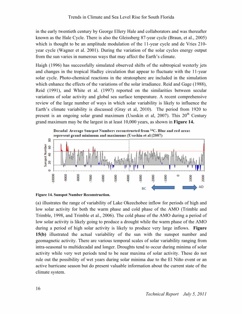
Trends in Climate and Sea Level Rise for South Florida
16 Technical Report July 5, 2011
in the early twentieth century by George Ellery Hale and collaborators and was thereafter known as the Hale Cycle. There is also the Gleissberg 87-year cycle (Braun, et al., 2005) which is thought to be an amplitude modulation of the 11-year cycle and de Vries 210-year cycle (Wagner et al. 2001). During the variation of the solar cycles energy output from the sun varies in numerous ways that may affect the Earth’s climate.
Haigh (1996) has successfully simulated observed shifts of the subtropical westerly jets and changes in the tropical Hadley circulation that appear to fluctuate with the 11-year solar cycle. Photo-chemical reactions in the stratosphere are included in the simulation which enhance the effects of the variations of the solar irradiance. Reid and Gage (1988), Reid (1991), and White et al. (1997) reported on the similarities between secular variations of solar activity and global sea surface temperature. A recent comprehensive review of the large number of ways in which solar variability is likely to influence the Earth’s climate variability is discussed (Gray et al, 2010). The period from 1920 to present is an ongoing solar grand maximum (Usoskin et al, 2007). This 20th Century grand maximum may be the largest in at least 10,000 years, as shown in Figure 14.
Figure 14. Sunspot Number Reconstruction.
(a) illustrates the range of variability of Lake Okeechobee inflow for periods of high and low solar activity for both the warm phase and cold phase of the AMO (Trimble and Trimble, 1998, and Trimble et al., 2006). The cold phase of the AMO during a period of low solar activity is likely going to produce a drought while the warm phase of the AMO during a period of high solar activity is likely to produce very large inflows. Figure 15(b) illustrated the actual variability of the sun with the sunspot number and geomagnetic activity. There are various temporal scales of solar variability ranging from intra-seasonal to multidecadal and longer. Droughts tend to occur during minima of solar activity while very wet periods tend to be near maxima of solar activity. These do not rule out the possibility of wet years during solar minima due to the El Niño event or an active hurricane season but do present valuable information about the current state of the climate system.

Natural Climate Variability
17 Technical Report July 5, 2011
Figure 15/ (a) Lake Okeechobee net inflow versus solar activity (CP) and AMO. (b) Solar activity represented by sunspot number (black) and geomagnetic activity (blue) (Trimble, P. and Trimble, B. (1998).
AMO Cold Phase
AMO Warm Phase (a)
(b)
Trends in Climate and Sea Level Rise for South Florida
18 Technical Report July 5, 2011
Variation of Tropical Storm Activity
According to the National Center for Atmospheric Research (2009) Florida tops all other states with the costliest damage due to extreme weather events through 2008. When ranked by event type, Florida was first in damage from hurricanes, fourth in flooding, and ninth in tornadoes. Tropical storms and hurricanes also contribute significant amounts of water to the state, which make them an important part of water management planning and assumptions.
The frequency of tropical storms and hurricanes changes as part of natural cycles that occur over decades. The Atlantic Basin is currently in a period of higher than average tropical storm activity due, for the most part, to a natural shift of the Atlantic Multi-decadal Oscillation from a cold phase to a warm phase (which occurred in 1995) and, to a much lesser extent, global climate warming (Florida Oceans and Coastal Council, 2009; Nyberg et al. 2007). In fact, the magnitude of changes in hurricane intensity due to global climate warming is of the order of one percent, which is not a significant or measurable amount (Pielke et al, 2005).
As the atmosphere warms, sea surface temperatures and wind shear will also increase. These two factors can have opposing effects on tropical storms. As the temperatures rise, more energy is available in the oceans and atmosphere for more rapid intensification of tropical storms and hurricanes. However, increased wind shear over the Atlantic Basin is expected to decrease the number of tropical storms and hurricanes in the Atlantic Ocean. In summary, according to Knutson et al, 2010, global warming has a potential to:
Decrease the number of tropical storm and hurricanes up to 6-34%.
Increase the wind intensity of the remaining hurricanes up to 2-11%.
Increase hurricane storm surge. The effects of future sea level rise due to global warming must also be considered and accounted for when considering estimations of the impact of expected storm surge.
Increased rainfall up to ~20% within 60 miles of tropical storms and hurricanes.
Change storm genesis regions and storm tracks to an uncertain degree, though large alterations are not indicated.
Potential Implications
If a decrease in the number of storms does occur, there may be significant changes to the distribution of rainfall, which will affect the water supply and natural ecology of south Florida. Longer periods between tropical storms may mean the region may be under drought conditions more often. A greater number of stronger hurricanes would increase the potential of damage to levees, canals, and other water control structures, resulting in an increased likelihood of flooding on a local and regional scale. Water supply and water quality may also be adversely affected by these more intense storms.

Historical Trends in Temperature and Precipitation
19 Technical Report July 5, 2011
III. Historical Trends in Florida Temperature and Precipitation
Introduction
The water resources management system in south Florida is among the most heavily managed in the world. Due to its low topographic relief, unique hydrology, and the large interannual variability of precipitation, south Florida is especially vulnerable to climate change.
The Fourth Assessment Report of the Intergovernmental Panel for Climate Change (IPCC) indicates that the vulnerability to climate change is mainly due to the increase in the frequency and intensity of extreme events rather than to gradual climate change, although gradual changes beyond certain thresholds can become significant (Parry et al., 2007). Due to increased water holding capacity in a warmer atmosphere, there is an increased chance for intense and heavy downpours to occur together with longer dry periods in between (Meehl et al., 2007; Trenberth et al., 2007) with potential repercussions to flooding and water supply aspects of water resources management.
Florida’s climate experiences natural variability of multiple scales, as evidenced by the dry and wet spells that can last for many years. The extent and timing of droughts have a profound effect on water availability in the system and limit water management flexibility with potential impacts to urban and agricultural users as well as the environment. For example, changes in precipitation frequency and intensity have been associated with long-term adverse impacts to ecosystems in south Florida (Shein, 2009). Warmer temperatures can result in reductions in dissolved oxygen and associated loss of fish and wildlife along with increased risk of coral bleaching (SFWMD, 2009). Climate change has the potential of exacerbating these conditions.
It therefore becomes important to understand the vulnerability of the water management system with respect to environmental restoration, water supply, and flood control due to future changes in climate. Climate change investigations should always be preceded by understanding the trends in historical climatic and other associated environmental data. We have investigated a comprehensive collection of climate metrics to study trends in both averages and extremes of precipitation and temperature in the state of Florida. The primary purpose is to investigate if there is a consistent regional trend in the statewide historical data. Although we make no formal attempt to attribute historical trends to natural or anthropogenic causes at this stage, there are instances in which the literature or the data show compelling evidence for attribution of trends to causes other than warming and those cases are briefly highlighted in the document.

Trends in Climate and Sea Level Rise for South Florida
20 Technical Report July 5, 2011
Due to varied influences, trends in long-term historical climatic data for Florida could be due to multiple factors. In addition to the effects due to global warming, changes in precipitation and temperature records could also be associated with natural cycles as well as feedback effects resulting from land use changes. Some of these factors as well as previous studies are described in the next section. Data quality is also an important consideration in attributing trends to climate change (Pielke et al., 2007).
Factors known to influence the climate of Florida were presented in Chapter II. In the next section, we present a summary of previous trend studies. We follow by describing sources and methods used for the analysis of historical climatic trends in the state. We finalize by summarizing results and presenting conclusions.
Previous Studies
Temperature Trends
Florida has undergone major changes in its landscape during the last century including the drainage of large wetlands to allow for urbanization and agriculture. In particular, agriculture has been migrating southward as a result of severe damaging freezes around the turn of the 20th century and in the 1980s. These severe freezes have been correlated with the Pacific/North American (PNA) teleconnections and the Arctic Oscillation (AO)/North Atlantic Oscillation (NAO) indices (Hagemeyer, 2007). Furthermore, regional climate modeling results suggest that increases in freeze severity and frequency may be due to conversion of south Florida wetlands to agriculture (Marshall et al., 2004b).
Urbanization has also dramatically altered the local climate. From an analysis of 57 weather stations for a 58-year period (1950–2007) in the state of Florida, Winsberg and Simmons (2009) found that the length of the hot season has increased at most locations. However, of the seven stations that had at least a three-week increase, five were in large cities and, therefore, Winsberg and Simmons (2009) attributed the “urban heat island” effect (urban areas tend to increase temperatures locally due to increased radiation of heat and reduced evaporation from asphalt surfaces, roofs, etc.) as the primary cause of the change in the length of the hot season. DeGaetano and Allen (2002) found statistically significant positive trends in extreme warm (probability [P] > 95th-percentile) minimum temperature exceedances (days) for some urban and suburban stations in Florida for the period 1930-1996 and especially for 1960-1996. They also found statistically significant decreasing trends in extreme cold (P< 5th-percentile) minimum and cold maximum temperatures exceedances, both pointing to warmer overall conditions. For the U.S. as a whole, they found that the trend in warm minimum temperature exceedances at urban stations is about three times that of rural stations, pointing to urbanization as a key driver of temperature variability.

Historical Trends in Temperature and Precipitation
21 Technical Report July 5, 2011
A study by Smith (2007) found mixed warming and cooling trends in deciles (a decile is one segment of a distribution that has been divided into ten groups having equal frequencies) of daily maximum temperature for Cooperative Observer (COOP) stations in the Florida peninsula for the period 1948-2004. Daily minimum temperature showed mostly significant warming trends across the state especially for the highest deciles. An exception is the Florida Panhandle, which showed significant cooling in the first (coldest) deciles of daily minimum temperature. Detailed examination of the station at the Apalachicola Municipal Airport by Smith showed significant warming in its maximum temperature deciles and significant cooling in its minimum temperature deciles, which Smith attributed to localized land cover changes and station relocation, respectively. This case study highlights the need for quality control of stations and the exclusion of stations with questionable data when analyzing region-wide temperature trends.
Kukla and Karl (1993) found that globally since the 1950s daily minimum temperatures have risen three times as fast as daily maximum temperatures resulting in a net decrease of the daily temperature range (DTR) as well as an increase in average temperature. Yow and Carbone (2006) found that the “urban heat island” in Orlando, Florida is more
marked (up to 8 C or 14.4 F) on calm clear nights when there is less vertical and horizontal mixing and the potential for greater rural cooling rates.
Based on correlation analyses, Snow and Snow (2005) analyzed 30-year trends in the annual temperature range (ATR) over the nine U.S. climate regions defined by the NOAA National Climatic Data Center (NCDC). The southeast region, which includes Florida, showed significant increasing trends in ATR for the period 1951-1980 with temperatures in the coldest month declining at a faster rate than temperatures for the warmest month of the year and both trends being statistically significant. The period 1961-1990 showed statistically insignificant increasing trends in ATR mostly driven by a statistically significant increase in warmest month temperatures. The period 1971-2000 showed a statistically insignificant decreasing trend in ATR which resulted from a statistically significant increase in warmest month temperatures together with a statistically insignificant increase in coldest month temperatures. This study highlights inter-decadal variability in temperature trends and suggests that since the 1960s temperatures for the warmest month have significantly increased in the southeastern U.S.
Coenen (2007) argues that due to the thermal inertia exhibited by lakes they are clearer indicators of medium-longer terms in temperature as opposed to air temperature measurements. His analysis of long-term records (1975-2004) at 50 lakes in Central Florida suggests a statistically significant (P<0.01) increase in wintertime lake water
temperature of approximately 1.0 +/- 0.9 C (1.8 +/- 1.6 F) over the period of record but no statistically significant changes in summertime temperature.
Maul and Sims (2007) using various sources of land air temperature, littoral water temperature and sea surface temperature (SST) found that Florida coastal air and water

Trends in Climate and Sea Level Rise for South Florida
22 Technical Report July 5, 2011
temperatures have increased by 0.2 to 0.4 C (0.4 to 0.7 F) over the past 160 years, but the statistical significance of the trend was found to be uncertain. Moreover, they found that the datasets yielded inconsistent results and no spatial pattern in the temperature change. They also strongly suggest that linear trends in highly cyclical data like temperature may be an artifact of the chosen analysis period.
It is evident from the above discussion that Florida temperatures are influenced by a variety of local/global and natural/anthropogenic factors. Temperatures in Florida are strongly influenced by the Gulf of Mexico and the Atlantic Ocean with the greatest effects near the coast (Fraisse et al., 2004). Several of the previously referenced studies also point to the urban heat island effect as a driver of local nighttime temperature increases especially evident on clear calm nights. There is evidence for teleconnections to global phenomena such as the PNA and the AO/NAO also having an effect on cold season temperatures. Due to the varied influences on Florida climate and weather, it becomes challenging to separate trends in temperature into natural versus anthropogenic drivers.
Precipitation Trends
Frich et al. (2002) analyzed changes in ten indicators of extreme climatic events for the second half of the 20th century. For the general vicinity of Florida, they found statistically significant decreases in maximum 5-day precipitation totals, a simple daily precipitation intensity index (annual total/number of days with ≥ 1 mm/day), and in the fraction of annual total precipitation due to events exceeding the 95th percentile for the period 1961-1990. Based on an analysis of 48 weather stations in Florida over the second half of the 20th century, Winsberg (2011) found no trends in the frequency of torrential rainfall (> 3 inches or 7.6 cm per day). However, he found that during La Niña phase of ENSO more torrential storms were produced than during the El Niño phase.
Nadarajah (2005) fitted generalized extreme value (Coles, 2001; Katz et al., 2002) distributions to annual maximum rainfall at 14 stations in west central Florida for the period 1901-2003. Different models for the location parameter were compared based on the likelihood ratio test including constant, linear, and quadratic trend models. The study found non-stationarity in annual maximum rainfall at eight of the stations with Orlando and Bartow showing downward linear trends. Clermont and Kissimmee showed upwardly concave quadratic trends, whereas Inverness, Plant City, Tarpon Springs and Tampa International Airport showed convex quadratic trends in the location parameter. The change point in the quadratic models usually occurred between 1940 and 1960. A decreasing linear trend in the location parameter was found at 12 of the 14 stations; however, it was only significant at two stations (Orlando and Bartow).
Using the Variable Infiltration Capacity (VIC) land surface hydrology model forced by NOAA-NCDC climate data and corrected for temporal heterogeneities, Andreadis and

Historical Trends in Temperature and Precipitation
23 Technical Report July 5, 2011
Lettenmaier (2006) simulated statistically significant increasing trends in drought severity over northeast and central-coastal Florida for the period 1915-2003.
It is evident from the above discussion that a variety of local/global and natural/anthropogenic factors influences Florida precipitation patterns. Wet season precipitation in Florida is driven by sea-breeze related convection and tropical systems, the latter of which is strongly influenced by the state of the AMO. A modeling study by Marshall et al. (2004a) indicates increased sea-breeze convergence and resulting slight increases in convective precipitation over urban areas along the eastern coast of south Florida resulting from urbanization. A large number of studies have identified the urban heat island effect as the cause of enhanced precipitation over and downwind of urban centers (Shepherd, 2005). The AMO, ENSO and PDO indices and their interactions have been tied to short-term and multi-decadal trends in central and south Florida precipitation patterns (Trimble et al., 2006). Due to the varied influences on Florida climate and weather, it becomes difficult to separate trends in precipitation into natural versus anthropogenic causes.
Data
The primary data investigated include long-term records of precipitation and raw (unadjusted) temperature. For this analysis, daily total precipitation (Precip), daily maximum (Tmax) and minimum (Tmin) surface temperature records at 32 stations distributed throughout the state of Florida are used (Figure 16, Table 4). These stations
Figure 16. Map of long-term precipitation and temperature stations used for historical trend analysis. Stations mentioned in the text are circled.
o Longitude
o L
atitu
de

Trends in Climate and Sea Level Rise for South Florida
24 Technical Report July 5, 2011
Table 4. Stations used for trend analysis.
COOP ID Station Latitude Longitude 80211 APALACHICOLA MUNI AP 29° 44' N 85° 01' W 80228 ARCADIA 27° 13' N 81° 52' W 80369 AVON PARK 2 W 27° 36' N 81° 32' W 80478 BARTOW 27° 54' N 81° 51' W 80611 BELLE GLADE 26° 41' N 80° 40' W 81046 BROOKSVILLE CHIN HILL 28° 37' N 82° 22' W 81978 CRESCENT CITY 29° 25' N 81° 31' W 82150 DAYTONA BEACH 29° 11' N 81° 04' W 82220 DE FUNIAK SPRINGS 1 E 30° 45' N 86° 05' W 82229 DELAND 1 SSE 29° 01' N 81° 19' W 82850 EVERGLADES 25° 51' N 81° 23' W 82915 FEDERAL POINT 29° 45' N 81° 32' W 82944 FERNANDINA BEACH 30° 40' N 81° 28' W 83163 FORT LAUDERDALE 26° 06' N 80° 12' W 83186 FORT MYERS PAGE FIELD 26° 35' N 81° 52' W 83207 FORT PIERCE 27° 28' N 80° 21' W 83470 GLEN ST MARY 1 W 30° 16' N 82° 11' W 84289 INVERNESS 3 SE 28° 48' N 82° 19' W 84570 KEY WEST INTL ARPT 24° 33' N 81° 45' W 84731 LAKE CITY 2 E 30° 11' N 82° 36' W 85275 MADISON 30° 27' N 83° 25' W 85879 MONTICELLO 5 SE 30° 34' N 83° 52' W 85895 MOORE HAVEN LOCK 1 26° 50' N 81° 05' W 86414 OCALA 29° 05' N 82° 05' W 86997 PENSACOLA REGIONAL AP 30° 29' N 87° 11' W 87020 PERRINE 4W 25° 35" N 80° 26' W 87025 PERRY 30° 06' N 83° 34' W 87205 PLANT CITY 28° 01' N 82° 09' W 87851 SAINT LEO 28° 20' N 82° 16' W 88758 TALLAHASSEE REGIONAL AP 30° 24' N 84° 21' W 88824 TARPON SPRINGS SWG PLNT 28° 09' N 82° 45' W 88942 TITUSVILLE 28° 37' N 80° 50' W
were obtained from the office of the state climatologists located at the Florida State University, and they constitute both National Weather Service (NWS) and Cooperative Observer (COOP) stations that have the longest and most complete daily precipitation and temperature records. Data for some of the stations go back to the year 1892 and end in 2008; however, the majority of stations have generally complete records starting in the 1950s. The data analyzed here are subject to quality control procedures; however, station moves, instrumentation changes and changes in the microclimate surrounding stations, which undoubtedly introduce inhomogeneities and may affect trends. Furthermore, adjustments to correct for those inhomogeneities may introduce spurious trends in the data (Pielke et al., 2007). Therefore, at least initially we chose to quantify trends in the raw (unadjusted) data.

Historical Trends in Temperature and Precipitation
25 Technical Report July 5, 2011
Trends in Precip, Tmax, and Tmin, daily average temperature (Tave), and daily temperature range (DTR) were analyzed for various relevant climate measures obtained from the literature (see for example Pielke and Downton, 2000; Frich et al., 2002). Daily average temperature (Tave) was estimated as the average of daily Tmax and Tmin, while the daily temperature range (DTR) was computed as the difference between daily Tmax and Tmin. Detection of trends in the measures listed in Table 5 was performed for annual
values, wet (warm) season –May, June, July + August, September, October (MJJ+ASO), dry (cool) season (NDJ+FMA), and three-month seasons (NDJ, FMA, MJJ, ASO). This partitioning into seasons is consistent with that used by Mestas-Nuñez and Enfield (2003) in their study on intra-seasonal to multi-decadal variability in south Florida rainfall. In addition to seasonal values, here we also examine trends in monthly totals or averages. Two periods were chosen for the trend analysis. First, trends were analyzed for the entire period of record (POR) at each station. Next, trends for the period 1950-2008 (post-1950) were analyzed. This latter period was chosen to investigate if the trends increase or decrease during the latter part of the period of record. The Fourth Assessment Report of
Table 5. Measures analyzed for trends.
Variable Averages (magnitude and duration, each by
season) Extremes (by season)
Precipitation Total precipitationa
Fraction of annual precipitation within a season
Number of wet daysb
Number of days of extreme values (> 1-in-2)c
Maximum seasonal value
Mean and maximum precipitation for events of duration 2, 3, 5, and 7 days
Number of heavy precipitation events (> 1-in-5)d of duration 2, 3, 5, and 7 days
Mean and maximum number of consecutive dry days
Daily temperature (average, maximum, minimum, daily temperature range)
Average temperaturea
Number of dog dayse
Annual temperature rangef
Number of days of extreme values (> 1-in-2)c
Maximum and minimum seasonal valuesg
Maximum values for events of duration 2, 3, 5, and 7 days
Number of extreme events (> 1-in-2)d of duration 2, 3, 5, and 7 days
a Also analyzed by month b Precip > 0.254 mm (trace precipitation) c Extreme days are defined as those exceeding the value corresponding to the 1-in-2 recurrence interval
for the corresponding seasonal maximum d Heavy precipitation events and extreme temperature events are defined as those exceeding the value
corresponding to a 1-in-2 recurrence interval for the maximum magnitude event of the specific duration N. N-day events that exceed the threshold but which have days overlapping other events exceeding the threshold are counted only once.
e Tave > 26.7 C f Computed as the difference between monthly maximum and monthly minimum of daily average
temperature g Applied to each of daily average, maximum, and minimum temperature, daily temperature range

Trends in Climate and Sea Level Rise for South Florida
26 Technical Report July 5, 2011
the IPCC (Trenberth et al., 2007) has reported an acceleration of mean temperature increase and sea level rise during the latter part of the last century and, therefore, the most recent period of record is inspected to see if such acceleration may be present in Florida temperature and precipitation records.
Methods
Although the presence of nonlinear trends is a distinct possibility, this initial work focuses on the presence or absence of linear trends, with year as the explanatory variable, except in the case of extremes (maxima and minima). The statistical significance of the slope parameter in the fitted linear model is tested using standard methods, which are briefly described below.
Different detection methods are better suited for detecting trends in different types of data. In our study, the non-parametric Mann-Kendall Trend Test (Mann, 1945; Kendall, 1938, 1976) and Sen-Theil Regression (Theil, 1950; Sen, 1968) were used for the majority of measures. The exception is extreme events for which Generalized Linear Modeling (GLM) of the parameters of the Generalized Extreme Value (GEV) Distribution was used.
The analysis presented here was performed in the R-programming (R Foundation for Statistical Computing 2008) environment (hereafter referred to as R) using available packages where possible. A significance level of 0.05 was used for all tests.
Mann-Kendall Trend Test and Sen-Theil Regression
The Mann-Kendall test, developed by Mann (1945) and Kendall (1938, 1976), is an alternative non-parametric trend test to ordinary least squares (OLS) regression. It is considered an improvement to OLS due to its resistance to outlier effects and influential data. It is also a robust test that is capable of detecting non-linear but monotonic trends and can be used with data that is non-normally distributed, and that contains missing or censored data.
The test consists of summing the signs of the difference between all pairs of sequential time series values
∑ ∑ (1)
where n is the length of the time series, Xj and Xk are sequential time series values for times tj and tk (j > k), and sgn is the sign function
1 0 0 0
1 0 (2)

Historical Trends in Temperature and Precipitation
27 Technical Report July 5, 2011
The null hypothesis (Ho) for the test is that the data, X, are a sample of n independent and identically distributed random variables (i.e. there is no trend, S = 0). The alternative hypothesis (Ha) states that the distribution of Xk and Xj are not identical for all k, j < n
and k j (i.e. there is a trend, S 0). The null hypothesis is rejected when S is significantly different from zero and there is a monotonic trend over time.
The Kendall package in R uses an algorithm developed by Best and Gipps (1974) to determine the statistical significance levels based on an Edgeworth expansion of the distribution of S (Silverstone, 1950; and David et al. 1951). When ties are present and n > 10, a normal approximation with continuity correction is used, in which the statistic Zs (defined below) is assumed to come from a standard normal distribution ~ N(0,1). The null hypothesis is rejected if |Zs| exceeds the critical value Zα/2 where FN (Zα/2) = α/2, FN being the standard normal distribution and α being the selected significance level. Unless ties are very extensive or the data is very short, this is an adequate approximation.
0
0 0
0
(3)
The standard deviation of S is given by Kendall (1976).
1 2 5 ∑ 1 2 5 (4)
where q is the number of tied groups and tp is the size of the pth tied group.
The Sen-Theil trend line (Theil, 1950; Sen, 1968) is a non-parametric alternative to linear regression that can be used in conjunction with the Mann-Kendall trend test. It does not require the assumptions of linear regression such as normality and constant variance of the residuals (homoscedasticity). However, it still assumes that residuals are statistically independent and that the relationship between the variables is linear. It can also handle missing and censored values.
The method consists of computing the simple pair-wise slope estimate: Skj = (Xj – Xk)/(tj – tk) for all possible distinct pairs of measurements, (Xk, Xj) where tj > tk. For a sample of size n, there will be N=n(n-1)/2 pairs of slopes. The Sen-Theil trend slope can then be computed as the median of all pair-wise slopes (b = median(Skj)), while the intercept of the trend line is given by a = median(X - bt). By taking the median pair-wise slope instead of the mean, extreme pair-wise slopes usually due to outliers have little impact, if any, on the final slope estimator.
The probability (P)-value for the computed Theil-Sen slope is obtained from the Mann-Kendall trend test. The slope estimate does not enter directly into the test procedure; therefore, small inconsistencies can occasionally arise between the computed slope and
Trends in Climate and Sea Level Rise for South Florida
28 Technical Report July 5, 2011
its associated P-value (McBride and Loftis, 1994). This is particularly true when there are many tied values as can be the case with count data.
The Mann-Kendall and Sen-Theil methods assume that the data are independent and identically distributed. However, if significant positive autocorrelation exists, the test tends to overestimate the significance of the computed trend and rejects the null hypothesis (Ho) of no trend more often than according to the selected significance level, i.e. it increases the type I (false positive) error (von Storch and Navarra, 1999). The opposite is true for the case of significant negative autocorrelation, where the test tends to underestimate the probability of detecting trends resulting in an increase in the type II (false negative) error (Yue et al., 2002).
The time series of precipitation and temperature measures analyzed here show significant positive autocorrelation much more frequently than negative autocorrelation. “Pre-whitening,” which is a mathematical process used to remove correlation, can be applied to remove positive serial correlation from the data. Many such methods are available in the literature (See von Storch and Navarra, 1995; Zhang et al., 2000; Wang and Swail, 2001; Yue et al. 2002; Petrow and Merz 2009). According to Matalas and Sankarasubramanian (2003), the effectiveness of pre-whitening decreases with decreasing lag-1 autocorrelation and sample size. As an alternative to pre-whitening, an effective sample size can be used with the Mann-Kendall test to account for serial correlation as described in Lettenmaier (1976), Hamed and Rao (1998), and Yue and Wang (2004). We chose to use the Zhang et al. (2000) iterative pre-whitening method as implemented in the zyp package in R. The method is described in Wang and Swail (2001). Finally, the Mann-Kendall test and the Sen-Theil slope can be computed for the pre-whitened time series.
The Mann-Kendall and Sen-Theil methods are only suitable for cases where the trend may be assumed to be monotonic and thus no seasonal or other cycle is present in the data. Seasonal versions of the Mann-Kendall trend test (Hirsch et al., 1982) and the Sen-Theil trend line have been developed to analyze trends in time series possessing a seasonal cycle. A modified version of the seasonal Mann-Kendall trend test which corrects for mild serial autocorrelation (i.e. autocorrelation from season to season but not for the same season across years) has been developed by Hirsch and Slack (1984). When the time series is actually independent, the Modified Seasonal Mann-Kendall trend test actually has less power to detect trends than the original Seasonal Mann-Kendall test. In our analysis, we first check whether the lag 1 autocorrelation coefficient for the deseasonalized monthly values is significant, and if it is, then we perform the Modified Seasonal Mann-Kendall trend test. Otherwise, we use the original Seasonal Mann-Kendall test.
The seasonal Sen-Theil trend slope estimator is derived from the non-seasonal estimator by computing all pair-wise slopes within each season and then gathering slopes from all

Historical Trends in Temperature and Precipitation
29 Technical Report July 5, 2011
seasons to determine the median slope. Although these seasonal tests are generally very robust, if there are opposing trends in different seasons then the power of the test will be greatly reduced because opposing trends will cancel out. The van Belle and Hughes test for trend homogeneity between seasons (i.e. months) (van Belle and Hughes, 1984) is carried out prior to application of the seasonal versions of Mann-Kendall and Sen-Theil. If the test shows that the data possess heterogeneous trends between seasons, then seasonal tests are not meaningful and the original trend tests (with pre-whitening) are performed on data for each individual season (month) of the year (i.e. 12 separate computations).
It is important to note that the Mann-Kendall Trend Test and Sen-Theil Regression have limitations when applied to data with many tied values as in the case of rare events for which a large number of counts are equal to zero. However, alternative methods such as generalized linear models also have difficulty in discriminating trends from stochastic fluctuations in time series of rare events. This is especially true for shorter time series, rarer events, and data sets that have smaller trend to noise ratios (see for example Frei and Schär, 2001; and Klein Tank and Können, 2003). For example, Frei and Schär (2001) found that using logistic regression the probability of detecting a 1.5-fold increase in the frequency of a 1-in-100 day event in a 100-year long record is only about 0.2. They caution that the non-significance of a trend in rare events does not necessarily imply the absence of a trend. As specified in Table 5, we chose to quantify trends in the number of extremes exceeding 1-in-2 of appropriate seasonal maxima, instead of rarer events such as a 1-in-5.
Trends in Extremes Based on the GEV Distribution
Based on Monte Carlo experiments Zhang et al. (2004) found that explicit consideration of the extreme value distribution in computing trends in extremes using generalized linear modeling always outperforms other methods such as OLS and Mann-Kendall even in the case of moderately serially correlated data. Therefore, in the case of extreme value variables (annual or seasonal maxima and minima), the data are fitted using the Generalized Extreme Value (GEV) distribution family given by (Coles, 2001; Katz et al., 2002):
/1
1exp)(z
zG (5)
where , , and are the location, scale, and shape parameters, respectively, of the GEV, which are fit to data by maximum likelihood using the ismev package in R. This distribution models maxima of a series of independent and identically distributed observations and is an appropriate distribution for analyzing extreme values. It encapsulates three distinct extreme value distributions by means of the shape parameter:
Trends in Climate and Sea Level Rise for South Florida
30 Technical Report July 5, 2011
Gumbel ( =0) which is light-tailed and unlimited, Fréchet ( > 0) which has a lower
limit and is heavy-tailed, and the reverse Weibull ( < 0) which has an upper limit at -
/ and is short-tailed. To model minima, z is replaced by (– z) in Equation (5) above.
The GEV parameters can be assumed as constant or expressed as a linear function of covariates in generalized linear modeling. Trends in extrema are investigated by assuming that the location parameter is a function of time, specifically the year. Nadarajah (2005) found that assuming trends in the scale and shape parameters in addition to the location parameter did not significantly improve the fit to historical annual
maximum rainfall for stations in west central Florida. Therefore, we chose to model
and as constants.
The null hypothesis (Ho) for the test is that there is no trend in the location parameter, while the alternative hypothesis (Ha) states that there is a trend in the location parameter. The significance of the trend in the location parameter is evaluated using the Likelihood Ratio Test, which uses the deviance statistic (Coles, 2001):
D = 2{l1(M1) – l0(M0)} (6)
where l1(M1) and l0(M0) are the log-likelihood function of the fitted models M1 (with trend in the location parameter) and M0 (without the trend in the location parameter), respectively. The test of the validity of one model against the other is based on the fact that the probability distribution of D can be approximated by the χ2 distribution with a degree of freedom for this case being equal to one. The null hypothesis is rejected when
D exceeds the critical value 2critα(df=1) for the selected significance level α.
Results and Discussion
The next subsections present detailed results from the trend analysis with emphasis on those variables and measures which show the most consistent and significant trends. Tables 6-10 summarize the results in terms of the number of stations (of the 32 stations listed in Table 4) with statistically significant trends in each of the temperature and precipitation measures analyzed based on the entire period of record at each station. Tables 11-15 show the same but for the post-1950 period only.
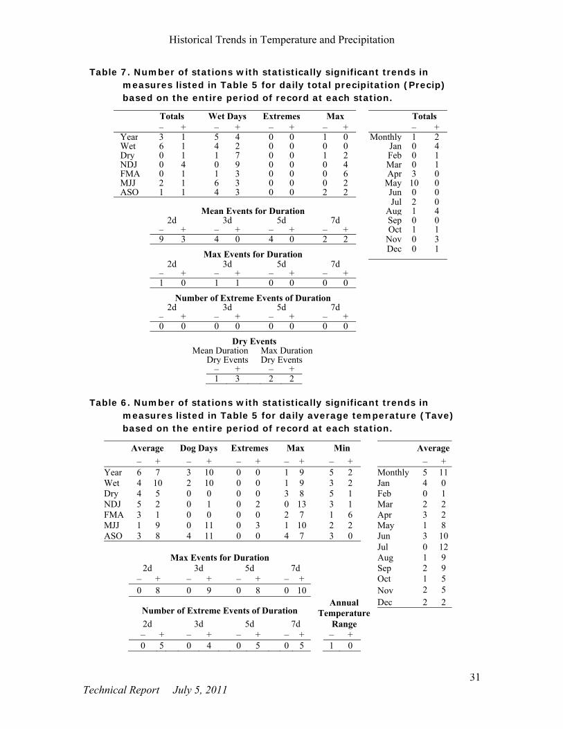
Historical Trends in Temperature and Precipitation
31 Technical Report July 5, 2011
Table 6. Number of stations with statistically significant trends in measures listed in Table 5 for daily average temperature (Tave) based on the entire period of record at each station.
Average Dog Days Extremes Max Min Average
– + – + – + – + – + – + Year 6 7 3 10 0 0 1 9 5 2 Monthly 5 11 Wet 4 10 2 10 0 0 1 9 3 2 Jan 4 0 Dry 4 5 0 0 0 0 3 8 5 1 Feb 0 1 NDJ 5 2 0 1 0 2 0 13 3 1 Mar 2 2 FMA 3 1 0 0 0 0 2 7 1 6 Apr 3 2 MJJ 1 9 0 11 0 3 1 10 2 2 May 1 8 ASO 3 8 4 11 0 0 4 7 3 0 Jun 3 10
Jul 0 12 Max Events for Duration Aug 1 9
2d 3d 5d 7d Sep 2 9 – + – + – + – + Oct 1 5 0 8 0 9 0 8 0 10 Nov 2 5
Number of Extreme Events of Duration Annual
TemperatureDec 2 2
2d 3d 5d 7d Range– + – + – + – + – + 0 5 0 4 0 5 0 5 1 0
Table 7. Number of stations with statistically significant trends in measures listed in Table 5 for daily total precipitation (Precip) based on the entire period of record at each station.
Totals Wet Days Extremes Max Totals – + – + – + – + – +
Year 3 1 5 4 0 0 1 0 Monthly 1 2 Wet 6 1 4 2 0 0 0 0 Jan 0 4 Dry 0 1 1 7 0 0 1 2 Feb 0 1 NDJ 0 4 0 9 0 0 0 4 Mar 0 1 FMA 0 1 1 3 0 0 0 6 Apr 3 0 MJJ 2 1 6 3 0 0 0 2 May 10 0 ASO 1 1 4 3 0 0 2 2 Jun 0 0
Jul 2 0 Mean Events for Duration Aug 1 4
2d 3d 5d 7d Sep 0 0 – + – + – + – + Oct 1 1 9 3 4 0 4 0 2 2 Nov 0 3
Max Events for DurationDec 0 1
2d 3d 5d 7d– + – + – + – +1 0 1 1 0 0 0 0
Number of Extreme Events of Duration2d 3d 5d 7d
– + – + – + – +0 0 0 0 0 0 0 0
Dry EventsMean Duration
Dry EventsMax Duration Dry Events
– + – +1 3 2 2

Trends in Climate and Sea Level Rise for South Florida
32 Technical Report July 5, 2011
Table 8. Number of stations with statistically significant trends in measures listed in Table 5 for daily maximum temperature (Tmax) based on the entire period of record at each station.
Average Extremes Max Min Average
– + – + – + – + – + Year 5 7 1 0 6 5 3 3 Monthly 7 11 Wet 3 9 0 0 8 4 3 8 Jan 3 0 Dry 3 5 0 0 5 5 4 4 Feb 0 5 NDJ 3 7 0 2 1 6 4 3 Mar 2 2 FMA 0 3 0 0 4 2 4 2 Apr 3 5 MJJ 3 8 0 2 2 5 2 10 May 1 5 ASO 4 7 0 0 8 3 3 4 Jun 2 6
Jul 2 10 Max Events for Duration Aug 2 8
2d 3d 5d 7d Sep 3 6 – + – + – + – + Oct 2 6 2 2 4 5 5 5 5 5 Nov 2 7
Number of Extreme Events of Duration
Dec 0 5
2d 3d 5d 7d – + – + – + – + 1 4 2 4 1 3 1 3
Table 9. Number of stations with statistically significant trends in measures listed in Table 5 for daily minimum temperature (Tmin) based on the entire period of record at each station.
Average Extremes Max Min Average
– + – + – + – + – +
Year 7 6 0 1 5 12 5 4 Monthly 10 11 Wet 5 11 0 0 4 12 8 4 Jan 8 0 Dry 8 3 0 1 1 9 5 3 Feb 0 1 NDJ 7 2 0 2 0 13 4 2 Mar 6 3 FMA 6 5 0 0 2 9 4 7 Apr 10 3 MJJ 5 11 0 1 2 14 6 9 May 6 6 ASO 6 7 0 3 6 10 5 2 Jun 4 12
Jul 4 10 Max Events for Duration Aug 4 12
2d 3d 5d 7d Sep 6 8 – + – + – + – + Oct 4 3 2 14 2 13 2 12 1 12 Nov 0 3
Number of Extreme Events of Duration
Dec 4 3
2d 3d 5d 7d
– + – + – + – +
1 9 1 9 1 6 0 7

Historical Trends in Temperature and Precipitation
33 Technical Report July 5, 2011
Table 10. Number of stations with statistically significant trends in measures listed in Table 5 for daily temperature range (DTR) based on the entire period of record at each station.
Average Extremes Max Min Average – + – + – + – + – +
Year 2 7 3 2 6 8 2 9 Monthly 10 11 Wet 4 7 0 1 6 5 2 8 Jan 2 7 Dry 1 8 2 2 6 12 2 9 Feb 2 7 NDJ 1 7 0 1 3 10 1 7 Mar 4 7 FMA 2 10 0 1 6 10 3 6 Apr 3 8 MJJ 5 4 0 2 7 5 4 11 May 3 7 ASO 3 6 0 2 3 8 2 11 Jun 6 2
Jul 6 6 Max Events for Duration Aug 8 5
2d 3d 5d 7d Sep 3 7 – + – + – + – + Oct 1 8 8 6 8 4 7 6 5 6 Nov 5 6
Number of Extreme Events of Duration
Dec 3 10
2d 3d 5d 7d– + – + – + – +4 2 4 2 3 3 1 5
Table 11. Number of stations with statistically significant trends in measures listed in Table 5 for daily total precipitation (Precip) based on the period 1950-2008.
Totals Wet Days Extremes Max Totals – + – + – + – + – +
Year 1 1 3 1 1 0 3 2 Monthly 2 2 Wet 1 1 3 1 1 0 3 2 Jan 0 3 Dry 0 0 1 2 0 0 0 1 Feb 1 0 NDJ 0 3 1 4 0 0 0 7 Mar 0 0 FMA 0 0 3 1 0 0 0 0 Apr 2 0 MJJ 1 1 2 1 0 1 1 2 May 7 0 ASO 0 1 4 1 2 0 3 0 Jun 0 1
Jul 2 1 Mean Events for Duration Aug 1 5
2d 3d 5d 7d Sep 0 1 – + – + – + – + Oct 5 1 2 2 2 1 1 1 1 3 Nov 0 4
Max Events for Duration
Dec 0 0
2d 3d 5d 7d– + – + – + – +2 0 2 1 0 0 0 1
Number of Extreme Events of Duration2d 3d 5d 7d
– + – + – + – +1 0 0 0 0 0 0 0
Dry EventsMean Duration
Dry EventsMax DurationDry Events
– + – +0 7 0 0

Trends in Climate and Sea Level Rise for South Florida
34 Technical Report July 5, 2011
Table 12. Number of stations with statistically significant trends in measures listed in Table 5 for daily average temperature (Tave) based on the period 1950-2008.
Average Dog Days Extremes Max Min Average– + – + – + – + – + – +
Year 3 9 4 8 0 2 2 8 0 4 Monthly 5 13 Wet 4 9 4 8 0 0 2 6 2 0 Jan 1 3 Dry 2 5 0 0 1 1 2 6 1 3 Feb 0 2 NDJ 0 5 0 0 0 2 0 15 0 2 Mar 0 1 FMA 2 3 0 0 1 0 6 3 3 0 Apr 4 1 MJJ 4 7 3 7 0 0 3 10 5 1 May 2 3 ASO 4 8 2 5 1 0 2 7 0 2 Jun 3 5
Jul 1 10 Max Events for Duration Aug 1 5
2d 3d 5d 7d Sep 2 8 – + – + – + – + Oct 1 5 0 5 0 5 1 5 1 7
Annual Temperature
Range
Nov 1 6
Number of Extreme Events of Duration Dec 0 3
2d 3d 5d 7d
– + – + – + – + – + 1 4 1 2 2 2 2 4 0 0
Table 13. Number of stations with statistically significant trends in measures listed in Table 5 for daily maximum temperature (Tmax) based on the period 1950-2008.
Average Extremes Max Min Average – + – + – + – + – +
Year 6 4 0 1 9 2 4 4 Monthly: 13 10 Wet 10 5 0 1 8 3 6 5 Jan 1 1 Dry 5 4 0 0 9 2 4 3 Feb 1 4 NDJ 3 3 0 1 3 4 2 1 Mar 2 3 FMA 4 5 0 0 9 2 5 0 Apr 4 2 MJJ 13 5 0 0 11 4 7 1 May 5 5 ASO 6 6 1 0 9 3 2 4 Jun 9 3
Jul 5 5 Max Events for Duration Aug 9 5
2d 3d 5d 7d Sep 3 5 – + – + – + – + Oct 2 5 5 3 5 3 7 4 8 3 Nov 1 5
Number of Extreme Events of Duration
Dec 0 3
2d 3d 5d 7d – + – + – + – + 0 3 0 3 0 2 2 3

Historical Trends in Temperature and Precipitation
35 Technical Report July 5, 2011
Table 14. Number of stations with statistically significant trends in measures listed in Table 5 for daily minimum temperature (Tmin) based on the period 1950-2008.
Average Extremes Max Min Average – + – + – + – + – +
Year 1 9 1 2 1 16 2 5 Monthly: 3 13 Wet 2 9 0 1 1 15 2 2 Jan 0 4 Dry 2 10 0 0 1 11 2 4 Feb 1 2 NDJ 2 8 0 1 0 20 0 7 Mar 1 5 FMA 3 5 1 0 2 5 1 3 Apr 5 1 MJJ 2 8 1 0 1 16 2 5 May 2 5 ASO 2 10 0 3 2 13 1 1 Jun 3 9
Jul 2 13 Max Events for Duration Aug 1 13
2d 3d 5d 7d Sep 1 6 – + – + – + – + Oct 1 5 2 14 1 13 2 14 2 14 Nov 0 6
Number of Extreme Events of Duration
Dec 0 4
2d 3d 5d 7d
– + – + – + – + 1 13 0 14 1 12 0 10
Table 15. Number of stations with statistically significant trends in measures listed in Table 5 for daily temperature range (DTR) based on the period 1950-2008.
Average Extremes Max Min Average – + – + – + – + – +
Year 7 2 0 0 9 7 11 2 Monthly: 15 6 Wet 10 3 2 2 11 4 6 3 Jan 6 3 Dry 7 5 1 3 9 6 8 1 Feb 7 5 NDJ 10 3 1 2 10 6 9 1 Mar 6 5 FMA 5 6 2 1 10 6 9 2 Apr 8 6 MJJ 11 3 2 2 11 2 12 2 May 9 5 ASO 9 3 0 2 7 4 3 3 Jun 11 2
Jul 14 4 Max Events for Duration Aug 16 2
2d 3d 5d 7d Sep 6 5 – + – + – + – + Oct 4 4
11 3 10 4 10 5 10 4 Nov 7 3
Number of Extreme Events of Duration
Dec 8 3
2d 3d 5d 7d
– + – + – + – + 4 4 6 3 7 4 6 5

Trends in Climate and Sea Level Rise for South Florida
36 Technical Report July 5, 2011
Precipitation
Results from the trend analysis show a general trend towards increasing precipitation at most stations in northern Florida and at coastal stations when the entire period of record (POR) is analyzed. However, only one station shows a statistically significant increasing trend at the 0.05 level. Interior areas of the state have generally seen a reduction in precipitation, but only three stations show it being statistically significant. The pattern of trends is less spatially coherent for the post-1950 period with trends at several stations reversing sign.
The majority of the decrease in precipitation at interior stations occurs during the wet season. This decrease in precipitation over interior areas is consistent with modeling results by Pielke et al. (1999) who found a decrease of June-July convective rainfall in interior areas of south Florida as a result of changes in land use from marshland to urban/agriculture that occurred from 1900 to 1993. In contrast, here we find that precipitation decreased throughout the state during the month of May with ten stations showing statistically significant declines when their entire POR is analyzed and seven stations showing statistically significant declines for the period post-1950 (Figure 17). It is possible that this decline in May precipitation may be tied to a general delay in the onset of the wet season. Preliminary analysis of data published by the National Weather Service (NWS; Lascody, 2002; Biedinger and Lushine 1993, 1998) on the onset of the wet season at three National Climatic Data Center (NCDC) stations located in Florida (Daytona Beach, Orlando, Miami) shows a general trend towards a delay in the onset of the wet season since 1935, though the trends are statistically non-significant. This is a subject that deserves additional investigation in the future.
When the entire POR is analyzed, there is a tendency for a decrease in 2-day mean precipitation with nine stations showing a statistically significant decline, but only three showing a statistically significant increase. However, this tendency is not seen when the post-1950 period is analyzed separately.
Another measure that showed some trend is the number of wet days during a season. Overall, four stations had statistically significant increases in the number of wet days during the entire year, while five stations had statistically significant decreases when the entire POR is analyzed. However, during the dry season (and specifically during NDJ) a relatively large number of stations (seven and nine stations, respectively) show statistically significant increases in the number of wet days (Figure 18). The same is not observed in the post-1950 period.
As mentioned earlier, trends in seasonal maxima and minima were determined by fitting a GEV distribution with and without the location parameter as a function of Year and using the likelihood ratio as a measure of significance. For seasonal maxima of precipitation, we found very little evidence of significant trends in the location parameter

Historical Trends in Temperature and Precipitation
37 Technical Report July 5, 2011
Figure 17. Trends in May precipitation for (a) the entire period of record, and (b) the 1950-2008 period. Triangles represent increasing trends, while circles represent decreasing trends. Filled markers represent trends significant at the 0.05 level.
(b)
(a)
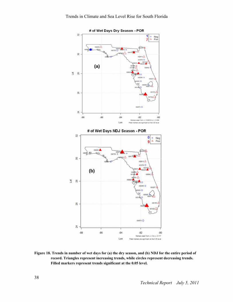
Trends in Climate and Sea Level Rise for South Florida
38 Technical Report July 5, 2011
Figure 18. Trends in number of wet days for (a) the dry season, and (b) NDJ for the entire period of record. Triangles represent increasing trends, while circles represent decreasing trends. Filled markers represent trends significant at the 0.05 level.
(b)
(a)

Historical Trends in Temperature and Precipitation
39 Technical Report July 5, 2011
fit to the entire POR. However, in general, the majority of the stations exhibited increasing trends in maxima for the dry season, NDJ, and FMA over their POR though most of these increasing trends were found to be non-significant. Only two stations showed statistically significant increases in dry season maxima, four stations had statistically significant increases in NDJ maxima, while six stations had statistically significant increases in FMA maxima. For the post-1950 period, most stations (except for south Florida) exhibited increases in NDJ maxima with statistical significance at seven stations. It is worth mentioning that the GEV fit at the great majority of the stations resulted in a positive shape parameter (i.e. Type II distribution-Pareto behavior in the tail) for all seasons (not shown). This agrees with Koutsoyiannis (2004 a,b) who showed that most time series of hydrological extremes follow a Type II distribution.
In terms of annual maxima, only one station exhibited a statistically significant decline for the entire POR. In contrast to the study by Nadarajah (2005) which found decreasing linear trends in the location parameter for annual maxima at 12 out of 14 stations in west central Florida, we could not find such a coherent spatial pattern in trends. Half of the eight west central Florida stations we analyzed showed negative trends while the other half showed positive trends in the location parameter for annual maxima. It is possible that this discrepancy between the two studies could be explained by the fact that in our analysis we included up to an additional decade at the beginning of the dataset (1892 vs. 1901 start period). It is worth noting, however, that Nadarajah (2005) also fitted positive shape parameters at these stations consistent with our findings.
We were also able to observe the multi-decadal trends in central and south Florida precipitation patterns and their relation to the Atlantic Multi-decadal Oscillation (AMO) as documented in Enfield et al. (2001), Obeysekera et al. (2006), and Trimble et al. (2006). A strong correspondence between a warm phase of the Atlantic Multi-decadal Oscillation (AMO) and increased regional precipitation is evident in the data. For the entire state of Florida, there is a switch in the sign of mean wet season precipitation anomalies between AMO cool years (1895-1925, 1970-1994) and AMO warm years (1926-1969, 1995-2008) from -2.4 cm/year to +1.6 cm/year (-0.9 to +0.6 in/yr), respectively, which is found to be significant at the 0.10 level. For the ASO season, the difference in mean precipitation anomalies (-3 cm/yr or -1.2 in/yr for AMO cool to +0.7 cm/yr or +0.3 in/yr for AMO warm) is found to be significant at the 0.05 level.
Temperature
Results from the trend analysis show an almost equal number of stations with statistically significant increases and decreases in daily average temperature (Tave) over the entire period of record (POR) at each station (seven and six stations, respectively). However, there appears to be a tendency toward an increased frequency of dog days (Tave > 26.7
C or 80 F). Ten stations showed statistically significant increases but only three showed statistically significant declines (Figure 19a). In contrast, for the post-1950 period, more

Trends in Climate and Sea Level Rise for South Florida
40 Technical Report July 5, 2011
Figure 19. Trends in annual number of dog days for (a) the entire period of record, and (b) the 1950-2008 period. Triangles represent increasing trends, while circles represent decreasing trends. Filled markers represent trends significant at the 0.05 level.
(b)
(a)

Historical Trends in Temperature and Precipitation
41 Technical Report July 5, 2011
stations show statistically significant increases than decreases in Tave (nine versus three), while the number of statistically significant increasing (decreasing) trends in the number of dog days is eight (four) (Figure 19b). Based on the entire POR, there is evidence of a non-significant increase in the annual temperature range (ATR) at two-thirds of the stations. However, this is not evident in the post-1950 period.
When the wet (warm) season is analyzed, it is found that Tave has increased at many locations (Figure 20a). For the entire POR, ten stations show statistically significant increase in wet season Tave, but only four stations show statistically significant decrease. This increase in wet season Tave is consistent with modeling results by Pielke et al. (1999) who found an increase of June-July temperatures (Tmax and Tmin), which has been attributed to changes in land use from marshland to urban/agriculture that occurred from 1900 to 1993. The changes in wet (warm) season Tave are consistent with changes in the number of dog days during the warm season, with ten stations showing statistically significant increases but just two stations showing statistically significant decreases (Figure 21a). This increase in the number of dog days during the wet season is apparent in both MJJ and ASO individually. When the post-1950 period is analyzed these patterns are somewhat less clear. Nine (four) stations show statistically significant increases (decreases) in wet season Tave (Figure 20b), while eight (four) stations show statistically significant increases (decreases) in wet season dog days (Figure 21b).
There is evidence for a warming of the hottest days with nine stations showing statistically significant increases in annual maxima Tave but only one station showing a significant decrease (Figure 22a) when the entire POR is analyzed. In particular, during NDJ and MJJ a great majority of stations show increases in seasonal maxima Tave with statistical significance at 13 and 10 stations, respectively (Figure 22b-c). This warming of the hottest days is also evident in increasing trends in the maximum 2 to 7-day hot spells at about two-thirds of the stations (statistically significant at 8-10 stations depending on hot spell duration), (Table 6). These general observations also hold for the post-1950 period (Figure 23). For the entire POR, a few stations (4-5) also showed statistically significant increase in the number of extreme 2 to 7-day hot spells; however, for the post-1950 period increasing trends were found at a larger number of stations but these were mostly non-significant. The average daily temperature during the hottest months of July and August has increased at a significant number of stations (12 and 9, respectively) for the entire POR. For the post-1950 period, Tave showed significant increases at ten stations during the month of July; however, the month of August did not show such consistent increases as during the entire POR.
Figure 24 presents the median (across 32 stations) annual station anomaly (deviation from the station mean) of daily average temperature. It is evident that there has been an overall increase in Tave over time for the state as a whole. However, it is possible that the overall increasing trend is at least partly due to multi-decadal shifts in temperature

Trends in Climate and Sea Level Rise for South Florida
42 Technical Report July 5, 2011
Figure 20. Trends in wet season average temperature (Tave) for (a) the entire period of record, and (b) the 1950-2008 period. Triangles represent increasing trends, while circles represent decreasing trends. Filled markers represent trends significant at the 0.05 level.
(a)
(b)

Historical Trends in Temperature and Precipitation
43 Technical Report July 5, 2011
Figure 21. Trends in number of dog days during the wet season for (a) the entire period of record, and (b) the 1950-2008 period. Triangles represent increasing trends, while circles represent decreasing trends. Filled markers represent trends significant at the 0.05 level.
(b)
(a)

Trends in Climate and Sea Level Rise for South Florida
44 Technical Report July 5, 2011
Figure 22. Trends in seasonal maxima of daily average temperature (Tave) for (a) the entire year, (b) the NDJ season, and (c) the MJJ season over the entire period of record. Triangles represent increasing trends, while circles represent decreasing trends. Filled markers represent trends significant at the 0.05 level.
(a)
(b)
(c)

Historical Trends in Temperature and Precipitation
45 Technical Report July 5, 2011
Figure 23. Trends in seasonal maxima of daily average temperature (Tave) for (a) the entire year, (b) the NDJ season, and (c) the MJJ season for the period 1950-2008. Triangles represent increasing trends, while circles represent decreasing trends. Filled markers represent trends significant at the 0.05 level.
regime due to natural causes or other factors. Although there is significant scatter in this data, it is clear from the smoothed trend line in Figure 24 that the regional temperature deviations experience an increasing trend up to about 1950 followed by a declining trend until about 1980. The more recent period since 1980 again shows an increasing trend. Fraisse et al. (2004) discuss how temperatures in Florida are strongly influenced by the Gulf of Mexico and the Atlantic Ocean with the greatest effects near the coast. Correlation analysis between median seasonal station anomaly of Tave and Atlantic or Gulf SST anomalies from NCDC Extended Reconstructed SST v3b (Smith et al., 2008) shows moderate to strong correlation coefficients ranging from 0.5 to 0.7 depending on the season (Table 16). All correlation coefficients were found to be highly significant with P-values practically equal to zero due to the large number of data values (117
(b)
(a)
(c)
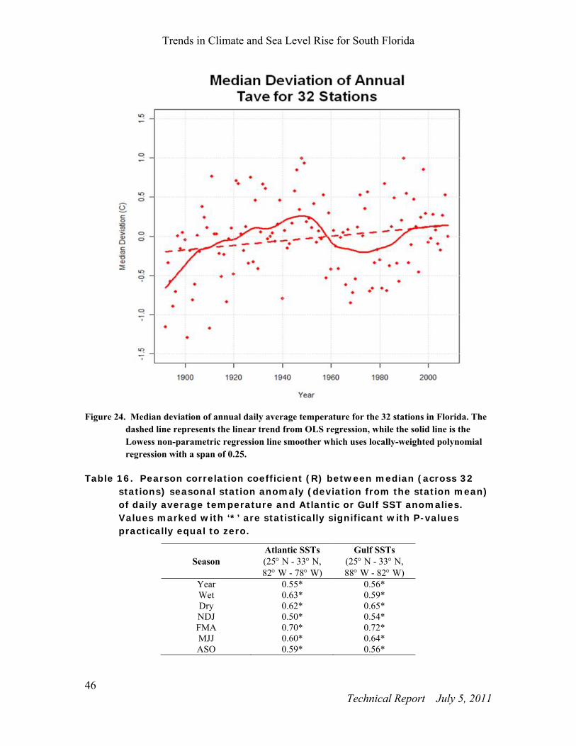
Trends in Climate and Sea Level Rise for South Florida
46 Technical Report July 5, 2011
Figure 24. Median deviation of annual daily average temperature for the 32 stations in Florida. The dashed line represents the linear trend from OLS regression, while the solid line is the Lowess non-parametric regression line smoother which uses locally-weighted polynomial regression with a span of 0.25.
Table 16. Pearson correlation coefficient (R) between median (across 32 stations) seasonal station anomaly (deviation from the station mean) of daily average temperature and Atlantic or Gulf SST anomalies. Values marked with ‘*’ are statistically significant with P-values practically equal to zero.
Season Atlantic SSTs (25 N - 33 N, 82 W - 78 W)
Gulf SSTs (25 N - 33 N, 88 W - 82 W)
Year 0.55* 0.56* Wet 0.63* 0.59* Dry 0.62* 0.65* NDJ 0.50* 0.54* FMA 0.70* 0.72* MJJ 0.60* 0.64* ASO 0.59* 0.56*

Historical Trends in Temperature and Precipitation
47 Technical Report July 5, 2011
seasonal values). The nonlinear trend pattern in Tave is characteristic of both U.S. and global trends (Hansen et al., 2000).
In terms of daily maximum temperatures (Tmax) over the POR, the only salient features are increasing trends during the months of July and August. For the month of July, 25 stations (80%) show increasing trends in Tmax with ten of those being statistically significant. For the month of August, 19 stations (60%) show increasing trends in Tmax with eight of those being statistically significant. Results for the post-1950 period show that wet (warm) season average Tmax decreased at 20 stations (significantly at 10 stations). This is especially evident during the months of MJJ when Tmax decreased at 21 stations (significantly at 13). With the exception of NDJ, seasonal maxima of Tmax decreased at over 20 stations for each season analyzed in the post-1950 period. As shown in Table 13, at least eight stations had statistically significant decreases in seasonal maxima for every season analyzed with the exception of NDJ. This is consistent with about two-thirds of stations showing a decrease in annual maximum 5 and 7-day average Tmax with seven and eight stations, respectively showing significant declines (Table 13).
The main conclusion from the POR analysis of trends in daily minimum temperatures (Tmin) is that seasonal maxima have increased at a large proportion of stations (Table 9). This is especially true for NDJ when 29 stations show positive trends, 13 of which are statistically significant. In all seasons, the number of stations with statistically significant positive trends in seasonal maxima (between 9 and 14) is more than double the number of stations with significant negative trends (between 0 and 6). These increasing trends in seasonal maxima are more evident in the post-1950 period where annual maxima increased at 26 stations (significantly at 16) and NDJ maxima increased at 31 stations (significantly at 20). The only season in the post-1950 period that did not show significant positive trend in maxima is FMA. A larger number of stations showed statistically significant increases than decreases in seasonal average Tmin for all seasons (except FMA) in the post-1950 period (Table 14). Average Tmin for the months of June, July and August in the post-1950 period increased at 25, 29 and 25 stations respectively, with corresponding statistically significant increases at 9, 13, and 13 stations. The maximum 2 to 7-day average Tmin also increased at about two-thirds of the stations for the entire POR and at 88% of stations (28) for the post-1950 period with the increase being statistically significant at over a dozen stations for both periods analyzed (Table 9 and Table 14). For the entire POR, a larger number of stations showed a statistically significant increase in the number of extreme 2 to 7-day hot spells; this was even more pronounced in the post-1950 period.
The number of stations showing statistically significant increases in the daily temperature range (DTR) exceeds the number of stations showing statistically significant decreases during the dry season, NDJ and FMA for the entire POR. This is consistent with the corresponding trends in Tmax and Tmin for the POR (Table 8 and Table 9). Stations in
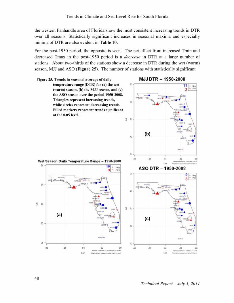
Trends in Climate and Sea Level Rise for South Florida
48 Technical Report July 5, 2011
the western Panhandle area of Florida show the most consistent increasing trends in DTR over all seasons. Statistically significant increases in seasonal maxima and especially minima of DTR are also evident in Table 10.
For the post-1950 period, the opposite is seen. The net effect from increased Tmin and decreased Tmax in the post-1950 period is a decrease in DTR at a large number of stations. About two-thirds of the stations show a decrease in DTR during the wet (warm) season, MJJ and ASO (Figure 25). The number of stations with statistically significant
(a) (c)
Figure 25. Trends in seasonal average of daily temperature range (DTR) for (a) the wet (warm) season, (b) the MJJ season, and (c) the ASO season over the period 1950-2008. Triangles represent increasing trends, while circles represent decreasing trends. Filled markers represent trends significant at the 0.05 level.
(b)

Historical Trends in Temperature and Precipitation
49 Technical Report July 5, 2011
decrease in DTR is between 9 and 11, while only three stations show statistically significant increase in DTR during the warm season, MJJ and ASO. Seasonal minima and to a lesser degree seasonal maxima of DTR has decreased at a large number of stations with more stations showing statistically significant decreases than increases in the post-1950 period. The months of June, July and August are the most notable with a much larger number of stations showing statistically significant decreases than increases in DTR (Table 15). Consistent with the above, the maximum 2 to 7-day average DTR decreased at a large number of stations with statistical significance for least at ten stations (Table 15).
As a side note, it is worth mentioning that the GEV fits to seasonal maxima of the temperature variables (Tave, Tmax, Tmin, and DTR) at the great majority of stations resulted in a negative shape parameter (i.e. Type III distribution – reverse Weibull behavior in the tail) for all seasons (not shown). This agrees with Kharin et al. (2005) who found that the distributions of annual temperature extremes tend to be short-tailed.
One of the most salient features in the temperature measures is the trend toward increased seasonal average Tmin for all seasons (except FMA) in the post-1950 period (Table 14) and the corresponding decrease in DTR (Table 15) at a large number of stations. The increasing trend in Tmin is consistent with trends observed globally since the 1950s when minimum daily temperatures have risen three times as fast as daily maximum temperatures (Kukla and Karl, 1993). According to Braganza et al. (2004) the observed reductions in DTR over the last century are large and unlikely due to natural variability alone. The debate over the cause for this decrease in DTR is far from settled. Various potential causes for this decrease in DTR include greenhouse warming and associated changes, increases in atmospheric aerosol concentrations, contrails, increased cloud cover at low-levels, increases in precipitation, irrigation and soil moisture, stable nighttime boundary layer dynamics, the urban heat island effect or a combination of these factors. Yow and Carbone (2006) found that the urban heat island in Orlando, Florida is more
marked (up to 8 C or 14.4 F) on calm clear nights when there is less vertical and horizontal mixing and the potential for greater rural cooling rates.
Pielke et al. (2007) also demonstrate that daily minimum temperatures on calm nights may be positively biased when measured at 2 m or so from the surface. This is because, measurement of Tmin at a single height does not capture the large vertical temperature gradients typical of light wind nights and, therefore, it is not representative of a boundary layer average value of temperature. Further, it does not well represent the heat content of the deeper atmosphere. Therefore, Pielke et al. (2007) suggest that only Tmax be used as a measure of large-scale climate change.
Due to the varied influences on Florida climate and weather, it is difficult to assign a unique cause for the decrease in DTR seen in the post-1950 period. However, analysis of grid-based population data developed by Owen and Gallo (2000) for United States

Trends in Climate and Sea Level Rise for South Florida
50 Technical Report July 5, 2011
Historical Climatology Network (USHCN) stations points to the urban heat island effect as a potential explanation for the decrease in DTR at some stations for the post-1950 period.
As an example, temperature trends for three stations with drastically different rates of population increase (Figure 26) are compared: Arcadia (80228) which is considered rural with a population of just over 15,059 (1990), Fort Myers Page Field (83186) which is a medium-sized coastal city with a population of 197,777 (1990), and Fort Lauderdale (83163) (1990 population: 671,460). Fort Lauderdale is on the opposite (east) coast from the other two stations and, for this reason, may be subject to different climatic influences.
Figure 26. Decadal population estimates for three USHCN stations in Florida. Population estimates were derived by Owen & Gallo (2000) for a 21 km by 21 km grid cell around each station.
As shown in Figure 27, during the period 1950-2008 DTR decreases the most at the most
populated station of the three analyzed (Fort Lauderdale with a 1.85 C or 3.3 F
decrease) and the least at the least populated station (Arcadia with a 0.35 C or 0.63 F
decrease) with Fort Myers having an intermediate decrease in DTR (0.84 C or 1.5 F decrease). From Table 17, it is evident that the relatively large decrease in DTR at the urban stations is due to a significant increase in Tmin, which also results in significant
increases in Tave and the number of dog days (Tave > 26.7 C or 80 F). This increase in Tmin at the most populated stations is consistent with the existence of more buildings retaining heat and blocking surface heat from radiating into the cold night sky by

Historical Trends in Temperature and Precipitation
51 Technical Report July 5, 2011
longwave radiation (McPherson, 1994). It is worth noting that although Tmax actually
increases at Fort Myers (by 0.77 C or 1.4 F), it is not enough to counteract a larger
increase in Tmin (1.58 C or 2.8 F) during this period.
Table 17. Trends (C and F or count of events over period 1950-2008) in temperature variables at three USHCN stations in Florida. Values marked with ‘*’ are statistically significant at the 0.05 level.
Variable/Station Arcadia (80228) Fort Myers
(83186) Fort Lauderdale
(83163)
Tave -0.22 C (-0.40 F) 1.14 C (2.05 F)* 0.98 C (1.76 F)* Tmax -0.17 C (-0.31 F) 0.77 C (1.39 F) -0.09 C (-0.16 F) Tmin -0.03 C (-0.05 F) 1.58 C (2.84 F)* 2.08 C (3.74 F)* DTR -0.35 C (-0.63 F) -0.84 C (-1.51 F) -1.85 C (-3.33 F)*
# of Dog Days -8 33* 27*
Figure 27. Trends in annual average daily temperature range (DTR) at (a) Arcadia, (b) Fort Myers, and (c) Fort Lauderdale for the period 1950-2008. The dotted line represents the linear trend from Sen-Theil regression with Zhang’s pre-whitening, while the solid line is the Lowess non-parametric regression line smoother which uses locally-weighted polynomial regression with a span of 0.25.
(c)
(b)
(a)
Trends in Climate and Sea Level Rise for South Florida
52 Technical Report July 5, 2011
Conclusions
Results of the trend analysis show a general decrease in Florida wet season precipitation over both the entire period of record at each station and the 1950-2008 period. This decrease in wet season precipitation is most evident for the month of May and is possibly tied to a delayed onset of the wet season in Florida. In contrast, there seems to be an increase in the number of wet days during the dry season, especially during NDJ, when the entire period of record is analyzed at each station.
In terms of temperature trends, we found that the number of dog days (Tave > 26.7 C or
80 F) during the year and during the wet season has increased at many locations. For the post-1950 period, a widespread decrease in the daily temperature range (DTR) is observed mainly due to increased daily minimum temperature (Tmin). Although we did not attempt to formally attribute these trends to natural versus anthropogenic causes, we infer that the urban heat island effect is at least partially responsible for the increase in Tmin and its corresponding decrease in DTR at urbanized stations compared to nearby rural stations.
This study represents an initial step in quantifying historical trends in temperature and precipitation over the state of Florida. This is key to understanding some of the potential impacts that climate change could have or might be having on regional water management. Future related research opportunities include investigation of inhomogeneities in the data due to station changes, consideration of non-linear trends, conducting a more formal trend attribution study, quantifying trends in parameters controlling evapotranspiration, and investigating changes in the onset and cessation of the wet and dry season.
Although the data analyzed here is subject to quality control procedures, station moves, instrumentation changes and changes in the microclimate surrounding stations undoubtedly introduce inhomogeneities, which may affect trends. Documentation on major station changes such as relocations and instrumentation changes can be readily obtained for most stations. However, the temporal history of changes in the local microclimate surrounding individual stations is generally lacking. These local microclimatic changes have the potential of introducing gradual changes in the data, which are difficult to detect and quantify. Furthermore, adjustments to correct for those inhomogeneities may introduce spurious trends in the data (Pielke et al., 2007). Therefore, at least initially we chose to quantify trends in the raw (unadjusted) data. In the future, raw and adjusted data at a station may be compared to better understand the homogeneity corrections being performed and their effect on trends. The representativeness of local measurements is also an important consideration in analyzing the data. For example, Pielke et al. (2007) demonstrate that daily minimum temperatures on calm nights may be positively biased when measured close to the surface. Therefore,

Historical Trends in Temperature and Precipitation
53 Technical Report July 5, 2011
they suggest that only Tmax be used as a measure of large-scale climate change. The computed trends may also be affected by the existence of cyclical patterns and the choice of analysis period.
In the future, a formal trend attribution study needs to be conducted for the region. Some attempts at separating global temperature signals from local effects include those of Kato (1996) and Karoly and Braganza (2005). Attribution has generally been based on climate modeling studies (Stott et al., 2004) or data-centric approaches (Schnur and Hasselmann, 2005; Lozano et al., 2009). Attribution becomes more difficult the smaller the spatial and temporal scales of analysis (Hegerl et al., 2007) so that it becomes harder to deterministically tie local or regional extreme events to natural versus anthropogenic causes. Rather, the increasing risk of such local extremes due to anthropogenic causes could be quantified (Stott et al., 2004).


Climate Projections
55 Technical Report July 5, 2011
IV. Climate Projections
Introduction
Planning investigations for Everglades Restoration and water needs of the urban and agricultural users require a large suite of metrics evaluated by planners, hydrologists, and biologists (www.evergladesplan.org). Generation of such metrics for future planning alternatives has required distributed, long-term simulation models of the system at finer scales than what is commonly used elsewhere. Much of the planning to date has been accomplished using a combined surface water/ground water model simulating both hydrologic processes and complex water management rules at a daily time step (SFWMD 2005) for the historical period of 1965–2005. The hydroclimatic drivers for this model are distributed rainfall and potential evapotranspiration interpolated on a 2 mile x 2 mile (3.2 km x 3.2 km) grid for the entire south Florida region using instrumental records of station rainfall, temperature, and other meteorologic parameters. In view of climate change projections (both natural and anthropogenic), the past use of the stationarity approach for planning requires an immediate update (Milly et al., 2008). Brekke et al. (2009a) recommend the use of paleoclimatic information (Kwon et al., 2009) and stochastic modeling for developing climate scenarios. However, methodologies for the generation of hydroclimatic information at the required spatial and temporal scales necessary for modeling associated with planning investigations in south Florida are not fully developed yet.
In this chapter, we explore the approach shown in Figure 28 (DWR, 2000) to investigate the skills and projections of both General Circulation Models (GCMs) and Regional Climate Models (RCM) for potential use in planning and operation of water resources management systems in south Florida.
Two primary datasets that will be used for this analysis: (a) observed climate data; and (b) a data set derived by combining General Circulation Models (GCMs) projections and downscaled, regional climate data for the Florida Peninsula. One of the first steps in this approach is to determine if the observed climate data shows any evidence that climate is changing in Florida, particularly during the latter part of 20th century. This aspect was already covered in Chapter III. Before GCMs and the regional information are used, a prudent practice is to assess their skills with respect to their performance during the 20th century by comparing the model results with observed data.
General Circulation Models
The generation of General Circulation Models (GCMs) reported in IPCC (2007a) provide a starting point for assessing the potential changes to climatic regime in the south Florida

Trends in Climate and Sea Level Rise for South Florida
56 Technical Report July 5, 2011
Figure 28. General approach used for using climate data and projections for water resources investigations.
region. The IPCC AR4 data for 23 models (Table 18) were downloaded from the International Research Institute for Climate and Society web site (http://iridl.ldeo.columbia.edu). These models are part of CMIP3 (Coupled Model Intercomparison Project Phase 3) developed by the IPCC Working Group. Data for the following scenarios were analyzed: (a) 20th Century Simulations (20c3m); Special Report on Emission Scenarios (SRES) B1 (low), A1B (midrange) and A2 (high). The variables used in this analysis are precipitation (pr), surface air temperature (tas), and daily maximum and minimum surface air temperature (tasmax and tasmin) at 2 meters. Twentieth century skills and the projections of GCMs were explored using monthly data which were available as continuous time series from 1850 to 2000.
Although GCMs provide long-range projections for the future, they have several weaknesses which discourage planners from using them directly in the evaluation of climate change impacts in water resources projects. The large spatial scales of the GCMs (100 km or more) are problematic for water resources planning investigations of local projects, and hydrologists often resort to downscaling of GCM data (Groves et al. 2008; Maurer et al. 2007; Nguyen and Nguyen 2008). Moreover, most GCMs do not completely agree in their future projections and no single model can be considered the best (Tebaldi et al., 2005). Different models perform well for certain metrics, but poorly for others. General Circulation Models provide reasonable simulation accuracy for global, hemispheric, and continental scales (Hewitson and Crane 1996; IPCC 2007c) and

Climate Projections
57 Technical Report July 5, 2011
Table 18. IPCC AR4 (Meehl et al., 2007) models used for the investigations of 20th century skills and assessing projections.
Originating Group(s) Country CMIP3 I.D. Abbrev.* Bjerknes Centre for Climate Research Norway BCCR-BCM2.0 BCM2 National Center for Atmospheric Research USA CCSM3 NCCSM
Canadian Centre for Climate Modelling & Analysis Canada CGCM3.1(T47)
Canadian Centre for Climate Modelling & Analysis Canada CGCM3.1(T63)
Météo-France / Centre National de Recherches Météorologiques
France CNRM-CM3 CNCM3
CSIRO Atmospheric Research Australia CSIRO-Mk3.0 CSMK3 Max Planck Institute for Meteorology Germany ECHAM5/MPI-OM Meteorological Institute of the University of Bonn,
Meteorological Research Institute of KMA, and Model and Data group.
Germany / Korea
ECHO-G ECHOG
LASG / Institute of Atmospheric Physics China FGOALS-g1.0 FGOALS US Dept. of Commerce / NOAA / Geophysical Fluid
Dynamics Laboratory USA GFDL-CM2.0 GFCM20
US Dept. of Commerce / NOAA / Geophysical Fluid Dynamics Laboratory
USA GFDL-CM2.1 GFCM21
NASA / Goddard Institute for Space Studies USA GISS-AOM GIAOM Institute for Numerical Mathematics Russia INM-CM3.0 INCM3 Institut Pierre Simon Laplace France IPSL-CM4 IPCM4 Center for Climate System Research (The University of
Tokyo), National Institute for Environmental Studies, and Frontier Research Center for Global Change (JAMSTEC)
Japan MIROC3.2(hires) MIHR
Center for Climate System Research (The University of Tokyo), National Institute for Environmental Studies, and Frontier Research Center for Global Change (JAMSTEC)
Japan MIROC3.2(medres) MIMR
National Center for Atmospheric Research USA PCM NCPCM *Abbreviation used in subsequent Tables and Figures
for seasonal and annual temporal scales, but errors become significant at finer spatial and temporal scales. They are generally more skillful in simulating temperature than precipitation (Hofstadter and Bidegain 1997; IPCC 2007c; USCCSP 2008) and in predicting mean conditions than variability. These limitations have prompted water resources analysts to look for general trends in the range of results coming from a multitude of models rather than one absolute projection from a single model (Brekke et al., 2008, 2009b). Due to the coarse resolution of most present-day GCMs, the region of south central Florida is not well represented. Some models do not represent large areas of the land mass of Florida or only represent it as mixed ocean/land cells. Most models only have one or two cells representing south central Florida with the highest-resolution model (MIHR) having about a dozen cells in the region. Therefore, it is expected that complex climatic spatial patterns resulting from mesoscale phenomena, such as sea and lake
Trends in Climate and Sea Level Rise for South Florida
58 Technical Report July 5, 2011
breezes, will not be adequately captured by these models. During the past decade, we have learned how natural climate variability in south Florida is driven by teleconnections to global phenomena, such as the Atlantic Multi-decadal Oscillation (AMO; Enfield et al., 2001), the El Niño Southern Oscillation (ENSO; Hanson and Maul, 1991), and the Pacific Decadal Oscillation (PDO; Mestas-Nuñez and Enfield 2003). The extent to which these phenomena and their teleconnections are adequately simulated by the GCMs dictates how well the natural climate variability of the region is simulated.
Before attempting to downscale coarse-scale GCMs, it is important to assess the reasonableness of the GCMs’ simulation of climatic regime of the south central Florida region. Here we present a comparison of the 20th century climate (20C3M scenario) simulation by various GCMs referenced in IPCC AR4. The purpose of the model validation is to identify which GCMs show higher skill in simulating the observed climatic regime in the region with the objective of using that information as a means for weighing their predictions of future climate change under increased greenhouse gas emissions (e.g. Murphy et al., 2004). A fundamental assumption in work to date is that the model that is more skillful in simulating the present climate will also provide more skillful predictions of the future climate.
The validation is limited to modeled fields of monthly total precipitation and monthly average surface temperature. We selected the Climatic Research Unit (CRU), University of East Anglia, UK – TS2.1 dataset (Mitchell and Jones, 2005; www.ipcc-data.org/obs/cru_ts2_1.html) as the observational dataset. The period chosen for comparison is 1961–1990. We first validated CRU TS2.1 for south central Florida by comparison against the National Climate Data Center climate division dataset (NCDC 2008). The CRU grid cell values within each GCM cell are averaged before each comparison. In the analysis presented here, only GCM cells that have a land-area fraction of over 50% are considered. The next sections provide a brief discussion of the results of the GCM model validation.
Precipitation
In order to simplify this initial GCM skill investigation, we first aggregated the monthly data into wet and dry seasons and compared them to the historical data. Figure 29 shows a comparison of box and whisker plots (hereafter referred to as box-plots) of dry- and wet-season precipitation of observed data set with those of different GCMs. The observational data set is larger because it is at a finer spatial resolution, whereas the data used for GCM model data may vary depending on its spatial resolution in the south Florida region. Although there is a difference between the number of data points in the observational data set and the GCMs, the box-plot comparison provides a high-level view of GCM skill in terms of bias and variability.

Climate Projections
59 Technical Report July 5, 2011
Figure 29. Comparison of the box-plots of GCM seasonal total precipitation with that of the observational dataset (Mitchell and Jones 2005) for ( a) the dry season, and (b) the wet season; (c) Comparison of the seasonal cycles of the observational precipitation compared to that of all GCMs.
(a) (b)
(c)

Trends in Climate and Sea Level Rise for South Florida
60 Technical Report July 5, 2011
The vast majority of models show a significant bias in the wet season (Figure 29b) and they do not possess the extremes that the observational data set includes. We believe that such an underestimation of wet season precipitation is due to the GCMs’ lack of skill in simulating sea-breeze-driven convective thunderstorm activity, which cannot be adequately captured by the coarse grid, although a higher-resolution model would not necessarily guarantee a more realistic simulation of such physical processes. The bias of GCMs during the dry season (Figure 29b) is much less than that of the wet season and their variability is comparable to that of the observational data set. This is also apparent in the comparison of the seasonal cycle of the observational data set and the GCMs (Figure 29c). In fact, the monthly climatology of some models are opposite in phase (Figure 30) compared to the observations.
Figure 30. (a) GCM cell for the MIMR model in central Florida region, and (b) the corresponding comparison of monthly climatology showing a significant phase shift
In order to compare the sample probability distributions of the observed dataset and the GCM results, the Kolmogorov–Smirnov (K–S) test (Massey, 1951) is conducted for each season (Table 19). The P-values for the K–S tests are tabulated for each model, and for each season with and without a correction for the means (anomalies in Table 19). It is clear from the small P-values for the case without correction for means that there is a significant difference between the sample distributions, although in some cases there is no significant difference during the dry season. However, when both wet season and dry season precipitation are corrected for bias, the distributions are quite comparable.
It is clear that there is a very poor representation of the seasonal cycle in the coarse-scale GCMs. While it is possible to correct for such biases in the downscaling techniques (Maurer and Hidalgo, 2008), it is not clear whether such a large bias-correction would produce reliable projections for future climate change scenarios. We also observe (not
(a) (b)
Longitude
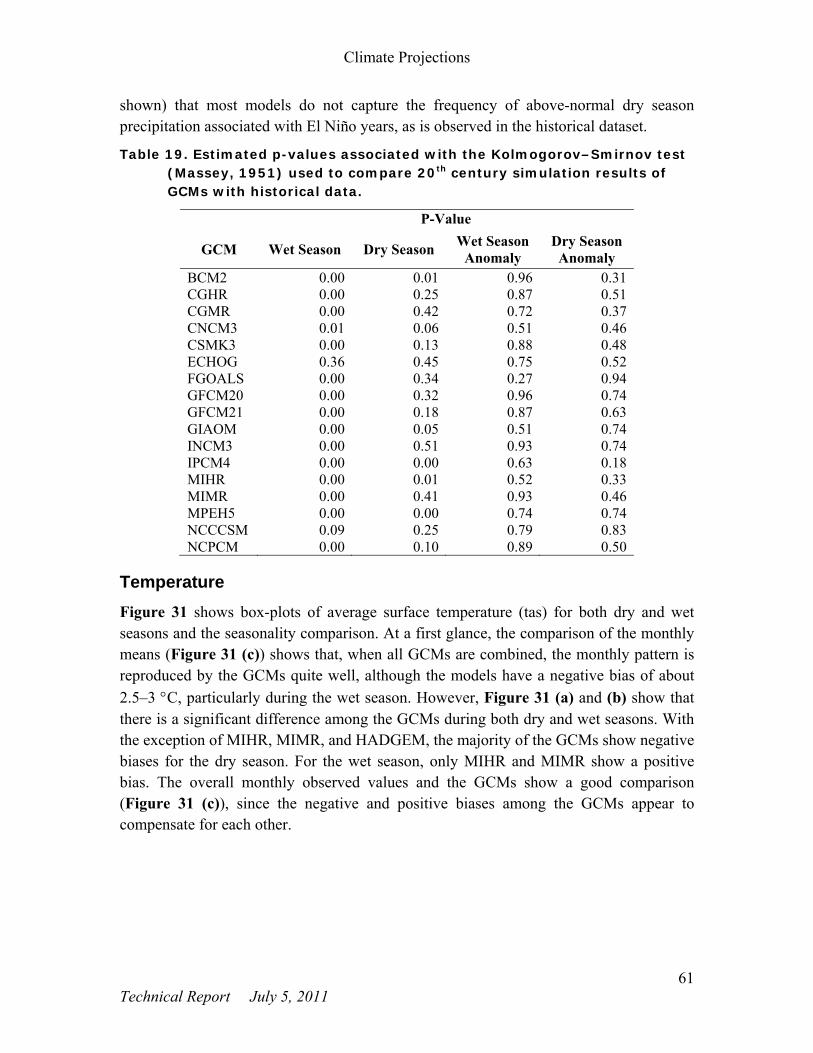
Climate Projections
61 Technical Report July 5, 2011
shown) that most models do not capture the frequency of above-normal dry season precipitation associated with El Niño years, as is observed in the historical dataset.
Table 19. Estimated p-values associated with the Kolmogorov–Smirnov test (Massey, 1951) used to compare 20th century simulation results of GCMs with historical data.
P-Value
GCM Wet Season Dry Season Wet Season Anomaly
Dry Season Anomaly
BCM2 0.00 0.01 0.96 0.31 CGHR 0.00 0.25 0.87 0.51 CGMR 0.00 0.42 0.72 0.37 CNCM3 0.01 0.06 0.51 0.46 CSMK3 0.00 0.13 0.88 0.48 ECHOG 0.36 0.45 0.75 0.52 FGOALS 0.00 0.34 0.27 0.94 GFCM20 0.00 0.32 0.96 0.74 GFCM21 0.00 0.18 0.87 0.63 GIAOM 0.00 0.05 0.51 0.74 INCM3 0.00 0.51 0.93 0.74 IPCM4 0.00 0.00 0.63 0.18 MIHR 0.00 0.01 0.52 0.33 MIMR 0.00 0.41 0.93 0.46 MPEH5 0.00 0.00 0.74 0.74 NCCCSM 0.09 0.25 0.79 0.83 NCPCM 0.00 0.10 0.89 0.50
Temperature
Figure 31 shows box-plots of average surface temperature (tas) for both dry and wet seasons and the seasonality comparison. At a first glance, the comparison of the monthly means (Figure 31 (c)) shows that, when all GCMs are combined, the monthly pattern is reproduced by the GCMs quite well, although the models have a negative bias of about
2.5–3 C, particularly during the wet season. However, Figure 31 (a) and (b) show that there is a significant difference among the GCMs during both dry and wet seasons. With the exception of MIHR, MIMR, and HADGEM, the majority of the GCMs show negative biases for the dry season. For the wet season, only MIHR and MIMR show a positive bias. The overall monthly observed values and the GCMs show a good comparison (Figure 31 (c)), since the negative and positive biases among the GCMs appear to compensate for each other.

Trends in Climate and Sea Level Rise for South Florida
62 Technical Report July 5, 2011
Figure 31. Comparison of the box-plots of GCM seasonal average temperature with that of the zonal dataset for(a) the dry season, and (b) the wet season; (c) comparison of the seasonal cycles of the observational temperature data with combined projections from all of the GCMs.
(a) (b)
(c)

Climate Projections
63 Technical Report July 5, 2011
GCM projections
It is clear from the analysis of the preceding sections that there is no single GCM dataset that could provide reasonably accurate precipitation and temperature projections for planning purposes for south Florida applications. It should be noted that GCM results for the 20th century do not correspond to a reproduction of historical data but rather they are plausible scenarios for the historical period. During this early stage of vulnerability analysis, we decided not to use a single model and a particular scenario. Instead, our approach is to use multiple scenarios using an ensemble of models with proper attention given to relative model credibility (Brekke et al., 2008). Using the Reliability Ensemble Average (REA) method, developed by Giorgi and Mearns (2002), as the basis, Tebaldi et al. (2005) developed a Bayesian approach for combining multi-model ensembles into a single probabilistic projection of either temperature or precipitation for a particular region. This projection is made by using weights based on model bias with respect to the current climate as well as a measure of model convergence, defined as the deviation of individual projection of change with respect to the central tendency of the ensemble of models (Tebaldi et al., 2005). In the Bayesian approach, observations for a particular region, X0, and the current and future precipitation or temperature values simulated by a GCM, Xi and Yi respectively, are assumed to follow the following model:
Likelihood:
Observed: X0 ~ N[μ, λ0-1] (7)
GCM (current): Xi ~ N[μ, λi-1]
GCM (future): Yi ~ N[ν, (θλi)-1]
Priors:
μ, ν ~ U(–∞,+∞ ) λi ~ Γ (a,b), θi ~ Γ (c,d)
where i denotes the model index, and N, U, and Γ refer to the Gaussian, Uniform, and Gamma distributions, respectively, with indicated parameters. The values of λi can be interpreted as a measure of model reliability and the posterior mean of this parameter is inversely proportional to bias in the particular model as well as the bias of the future prediction compared to the overall mean of all models [see Equation (9) in Tebaldi et al. (2005)]. Consequently, the concept of model bias as well as the “convergence” is directly linked to this relationship of the posterior mean of λi.
In other applications of the multi-model ensemble approach, several metrics have been proposed for different planning objectives (Brekke et al. 2008). In Tebaldi et al.’s approach, the two measures, Bias and Convergence, are assumed to reflect the model reliability in terms of its skill in reproducing historical observations as well as consistency with future projections of the entire ensemble. Although a more elaborate

Trends in Climate and Sea Level Rise for South Florida
64 Technical Report July 5, 2011
formulation of a Bayesian model is possible, it is beyond the scope of the current phase of the vulnerability analysis. The approach proposed by Brekke et al. (2008) will likely be required for incorporation of climate information for the future planning of water resources projects in south Florida.
In order to obtain a probability distribution of GCM projections specific to the south Florida region, we obtain the Regional Climate Change projections from multi-model ensembles made available via the National Center for Atmospheric Research (http://rcpm.ucar.edu). Regional Climate Change projections have been pre-computed for many regions around the world, including many parts of the United States. Although the results for the southeastern United States are available, a special simulation for a grid covering only a region which largely includes the eastern portion of the Florida peninsula (Figure 32) and some coastal cells north of Florida is obtained for this study. A minimum number of four cells are required for the Bayesian approach (see http://rcpm.ucar.edu) and, therefore, a cell off the coasts of Georgia and South Carolina is added to the grid region. Since the purpose of this initial effort is to determine reasonable estimates of potential changes in precipitation and temperature, the selection of the particular region is not expected to be very critical. The Bayesian model is used to develop probability distributions of both temperature and precipitation for SRES emission scenarios A2 (high), A1B (midrange), and B1 (low), as described in the IPCC (2007a) report. The monthly probability distributions are then used to obtain a reasonable range of precipitation and temperature changes that can be expected for the year 2050.
Figure 31(b) and (c) show the 5th and 95th percentiles of the posterior distributions of temperature and precipitation changes, respectively. The distributions are the results of the Bayesian approach providing higher weights for models according to the aforementioned bias and consistency criteria. Figure 33 shows an example of the posterior distributions which also includes the GCM data for comparison.
Results of Figure 31 show that there is a definite seasonality in the temperature change projected for 2050, with summer months (June through October) showing larger increases than other months. It is also evident that there are very few negative values, confirming the general warming that has been projected for the emission scenarios. A median projection of 1–1.5 ºC with a range of 0–2.5 ºC is a reasonable temperature change that could be expected for 2050 in this region. In contrast, precipitation projections have a wider range (–20% to +30%) with a significant proportion of negative values. It is clear that there is a larger spread in wet season months and that there is no clear indication of the sign of precipitation change (–ve or +ve). Nevertheless, these probability distributions provide reasonable estimates of precipitation and temperature change that could be expected for the south Florida region for preliminary planning investigations.

Climate Projections
65 Technical Report July 5, 2011
Figure 32. (a) Region used for Bayesian averaging of multi-model ensembles; and (b) the temperature; and (c) precipitation, and projections for 2050. In each graph, 5th and 95th percentiles corresponding to B1, A1B, and A2 scenarios (red, black and blue bar, respectively) for each month are plotted. Precipitation projection is expressed as a percentage.
Figure 33. Posterior distribution of temperature change (A2 scenario) for year 2050 and the month of June. Also shown are corresponding GCMs, whose weighted projections collectively produce the probability distribution.
(a) (b)
(c)

Trends in Climate and Sea Level Rise for South Florida
66 Technical Report July 5, 2011
Regional Climate Models
As illustrated above, the spatial scale of General Circulation Model output is too coarse for most regional water resources investigations. Multiple downscaling approaches exist for deriving regional climate from coarse resolution model output and they generally fall into two categories: (a) Statistical Downscaling and (b) Dynamical Downscaling.
Validation of Statistically Downscaled Climate Data
In this section, we explore the skills and projections of a statistically downscaled dataset available for the entire United States. The data set consists of 112 fine-resolution climate projections, based on 15 climate models and the SRES scenarios B1, A1B, and A2 at a monthly time-scale for the period 1950-2099 (Maurer et al., 2007). The spatial resolution of the data set is 1/8◦. The data is available as statistically downscaled GCM data derived using a methodology known as Bias Correction Spatial Disaggregation (BCSD), originally developed by Wood et al. (2004) and used extensively for water resources investigations in the recent years (e.g. Maurer, 2007). In this method, bias-correction is achieved by using a quantile-based mapping technique at 2◦, common to all GCMs, followed by a spatial downscaling step to interpolate data to the 1/8◦ scale.
As shown in Figure 28, one of the prerequisites for using regional climate projections is the validation of the 20th century simulations against the historical data. Figure 34 shows the grid points of the BCSD data corresponding to south central Florida region. Also shown are 26 historical gauge locations for both temperature and precipitation which were used to validate the 20th century BCSD data.
BCSD data for the 20th century simulations were compared with the historical data at each of the 26 locations shown in Figure 34. Statistical downscaling of the 20th century GCMs simulations provide valuable information for verifying the methodology used to predict future temperature and precipitation at a higher resolution (1/8 degree in this case) from a much coarser GCM grid dataset. Because GCM results for the 20th century represent plausible scenarios rather than a reproduction of historical data, it is incorrect to perform a straight correlation analysis of historical data versus 20th century downscaled data. For this investigation, the ability of the downscaling to reproduce the climatology was investigated by comparing the box and whisker plots of the 20th century data with the corresponding historical data at each location (Figure 35 and Figure 36).
It is clear from Figure 35, the bias correction has worked extremely well for temperature. Both the historical seasonal pattern and the monthly variability of temperature at each location are mimicked by the 20th century data produced by statistical downscaling. Since bias correction methodology is expected to reproduce the temporal distribution, this result was expected. However, Figure 36 shows that, in the case of precipitation, the bias correction has not worked well for all months. In particular, during the summer months

Climate Projections
67 Technical Report July 5, 2011
at most locations, downscaled data appear to underestimate the historical means. Further, the variability of the simulated data during the summer months appears to be lower than that of the historical data. The BCSD methodology does not use an identical methodology for the bias correction of temperature and precipitation and in the case of the latter the method is unable to reproduce the magnitude of the seasonal means, although the general seasonal pattern appears to be well preserved. The underestimation of the precipitation during the summer months may have undesirable consequences when the downscaled data is used in water resources investigations.
Figure 34. BCSD data grid and the stations and their locations used to validate the 20th century simulations.

Trends in Climate and Sea Level Rise for South Florida
68 Technical Report July 5, 2011
Figure 35. Comparison of monthly box-and-whisker plots of temperature for the 20th century.
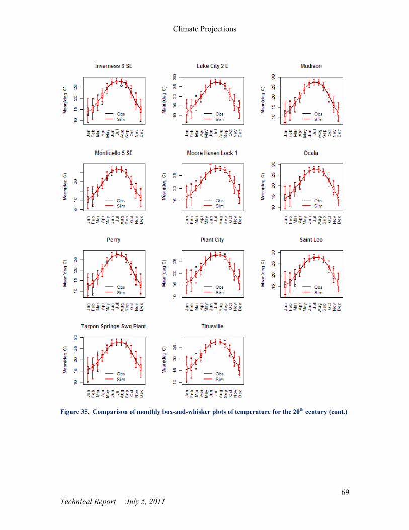
Climate Projections
69 Technical Report July 5, 2011
Figure 35. Comparison of monthly box-and-whisker plots of temperature for the 20th century (cont.)

Trends in Climate and Sea Level Rise for South Florida
70 Technical Report July 5, 2011
Figure 36. Comparison of monthly box-and-whisker plots of precipitation for the 20th century.

Climate Projections
71 Technical Report July 5, 2011
Figure 36. Comparison of monthly histograms of precipitation for the 20th century (cont.)
Projections of Statistically Downscaled Data
Future changes to water supply in south Florida depend heavily on precipitation patterns and evapotranspiration losses of the 21st century. Temperature is a major parameter that influences evapotranspiration losses, although several other meteorological and physiological variables also determine its magnitude. For planning of water resources during the 21st century, it is important to understand the general magnitude of the changes that could be expected for both precipitation and temperature. Mean monthly and mean annual values of both temperature and precipitation for the entire period (1950-2100)

Trends in Climate and Sea Level Rise for South Florida
72 Technical Report July 5, 2011
were plotted for each station and the Scenarios B1 and A2. To facilitate the discussion of the results, monthly and annual temperature plots for B1 and A2 scenarios for the Everglades station are shown in Figure 37 and Figure 38.
Figure 37. Monthly (left) and annual temperature patterns of BCSD models corresponding to the B1 scenario for the Everglades location. Also shown are historical observed (red dots) and historical simulated (black dots) for the same location.
Figure 38. Monthly (left) and annual temperature patterns of BCSD models corresponding to the A2 scenario for the Everglades location. Also shown are historical observed data for the same location (red dots) and historical simulated data (black dots).
Also shown are the historical observed and simulated data for the same location for the common overlapping period during the 20th century. As seen on these figures, historical data is available for the period prior to 1950 in some locations. Multiple traces (with differently colored symbols) show different models that were used in downscaling. Historical data generally compare well with BCSD data for the 20th century, as expected.
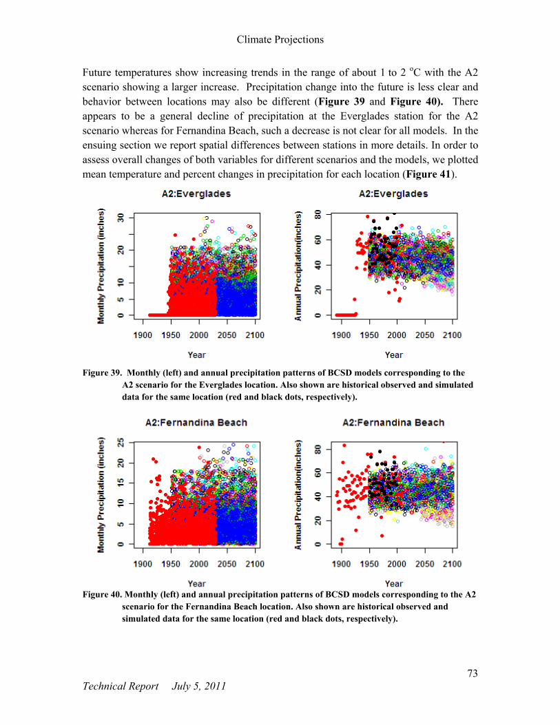
Climate Projections
73 Technical Report July 5, 2011
Future temperatures show increasing trends in the range of about 1 to 2 oC with the A2 scenario showing a larger increase. Precipitation change into the future is less clear and behavior between locations may also be different (Figure 39 and Figure 40). There appears to be a general decline of precipitation at the Everglades station for the A2 scenario whereas for Fernandina Beach, such a decrease is not clear for all models. In the ensuing section we report spatial differences between stations in more details. In order to assess overall changes of both variables for different scenarios and the models, we plotted mean temperature and percent changes in precipitation for each location (Figure 41).
Figure 39. Monthly (left) and annual precipitation patterns of BCSD models corresponding to the A2 scenario for the Everglades location. Also shown are historical observed and simulated data for the same location (red and black dots, respectively).
Figure 40. Monthly (left) and annual precipitation patterns of BCSD models corresponding to the A2
scenario for the Fernandina Beach location. Also shown are historical observed and simulated data for the same location (red and black dots, respectively).

Trends in Climate and Sea Level Rise for South Florida
74 Technical Report July 5, 2011
Figure 41. Change in temperature and percent precipitation from 1971-2000 to 2041-2070.

Climate Projections
75 Technical Report July 5, 2011
Figure 41. Change in temperature and percent precipitation from 1971-2000 to 2041-2070 (cont.)

Trends in Climate and Sea Level Rise for South Florida
76 Technical Report July 5, 2011
Figure 41. Change in temperature and percent precipitation from 1971-2000 to 2041-2070 (cont.)
Review of the plots in Figure 41 shows that, in general, the range of temperature change during the next 50 years is about 1-2 oC. Further, the B1 scenario shows the lowest increase and the change in A1 and A2 scenarios are generally similar. There are some models which are outliers showing a different pattern as compared to the rest of the models (points in the extreme second quadrant) and, most likely, these models should be discarded from any future use. In the case of precipitation, change during the next 50 years could be generally in the range of -10% to +10%. However, the sign of the magnitude of change appears to depend on the location. In some locations, the changes appear to spread around 0% whereas at other stations the percent change is more biased toward positive values.
In order to investigate the spatial trends in the expected changes by 2041-2070, changes in both temperature and percent precipitation were sorted by increasing latitude and plotted (Figure 42 and Figure 43). This analysis shows that there is a clear trend in both temperature and precipitation from south to north (i.e. increasing latitude). For the B1 scenario, average temperature increase is in the range of 1.0 to 1.5 oC, with the magnitude increasing with latitude (Figure 42). For both A1B and A2 scenarios, the increases appear to be in the range of 1.5 to 2.0 oC, again with a similar trend according to the latitude. Figure 43 shows that within the south Florida region (from the Everglades station to the Arcadia station), the net precipitation change seems to fluctuate around 0%, whereas for all other areas in the north, the results show a more positive bias in the precipitation change. The above analysis suggests that areas south of Lake Okeechobee, the net precipitation change could be positive or negative where in the areas to the north future climate may show more of an increase in precipitation.

Climate Projections
77 Technical Report July 5, 2011
Figure 42. Box and whisker plots of temperature change from 1970-1999 to 2041-2070 sorted by
increasing latitude.

Trends in Climate and Sea Level Rise for South Florida
78 Technical Report July 5, 2011
Figure 43. Box and whisker plots of precipitation change from 1970-1999 to 2041-2070 sorted by increasing latitude.

Climate Projections
79 Technical Report July 5, 2011
Dynamically Downscaled Climate Data
Precipitation and evapotranspiration are the two most important predictors of the amount of water available for planning investigations of future projects designed to meet the needs of urban, agricultural, and natural systems of Florida. Although General Circulation Models (GCMs) provide long-range projections for the future, due to their coarse scales and the inability to represent the Florida peninsula well, the projections from these models are not sufficiently reliable for planning and operation of large-scale projects (Obeysekera et al., 2010). Although higher-resolution, statistically downscaled precipitation and temperature projections are available (previous section), there is no guarantee that such information can adequately represent complex spatial patterns associated with mesoscale phenomena of the region, and the potential linkages to such teleconnections as El Niño-Southern Oscillation (ENSO) and Atlantic Multi-decadal Oscillation (AMO).
An alternative to statistical downscaling is to use a Regional Climate Model (RCM) to interpolate GCM projections to a higher resolution grid within a particular region. Such models are driven by the coarser GCM output as boundary conditions to simulate climate variables on a higher resolution regional grid using a regional model which includes the relevant physical processes in a limited area. Recently, there have been many efforts to develop and apply RCMs for dynamical downscaling but availability of such models for general use, particularly in Florida, is limited.
Recently, the National Center for Atmospheric Research (NCAR) has developed a program called the North American Regional Climate Change Assessment Program (NARCCAP) to produce high resolution climate change simulations for use in impact research. This is an international program with participation by many modeling groups who are running RCMs driven by a set of Atmosphere-Ocean General Circulation Models (AOGCMs) over a domain covering the conterminous United States and most of Canada. Currently, GCMs forced by the SRES A2 (high) emissions scenario for the 21st century have been used by the RCMs to produce a set of future projections. Also available are the corresponding simulations for the 20th century. The RCMs are nested within the AOGCMs for the current period 1971-2000 and for the future period 2041-2070. All the RCMs are run at a spatial resolution of 50 km.
We have investigated the ability of one of the NARCCAP models to simulate the spatial and seasonal patterns of both precipitation and temperature. Using the Penman-Monteith model of evapotranspiration (ET), together with maximum and minimum temperature, incoming solar radiation, wind, and humidity variables of the NARCCAP model, we have also investigated the magnitude of the derived estimates of reference grass evapotranspiration (RET) and compared them with the spatial and point estimates of RET based on observations. Physiological changes in vegetation due to increased CO2 concentrations (CO2 fertilization) and associated changes in photosynthesis and ET rates

Trends in Climate and Sea Level Rise for South Florida
80 Technical Report July 5, 2011
are not addressed at this moment, but could result in large changes in crop requirements and the water balance of the region (see USCCSP, 2008 for example).
Data and Methods
The NARCCAP program makes data available for several RCMs driven by the boundary conditions of corresponding GCMs (Figure 44). For this initial investigation, both daily and three-hourly variables from NARCCAP data tables (http://www.narccap.ucar.edu/) for the Canadian Regional Climate Model (CRCM) driven by the Third Generation Couple Global Climate Model (CGCM3) were used.
Figure 44. NARCCAP model structure. Shaded boxes indicate the GCM and corresponding RCM used for this investigation.
Most of the data handling and analysis was conducted using scripts written in R-language (The R Foundation for Statistical Computing, 2008) and the R-package (Fields, 2006). In a few cases, the National Center for Atmospheric Research Center’s Command Language (NCAR-NCL, 2011) scripts were used to estimate variables using fundamental variables that are available from the NARCCAP dataset. In particular, the following variables were used for this investigation:
• NARCCAP Table 1: Maximum & Minimum Daily Surface Air Temperature (tasmax & tasmin) at 2 meters
• NARCCAP Table 2: Surface Specific Humidity (huss), Precipitation (pr), Average Surface Pressure (ps), Surface Downwelling Shortwave Radiation (rsds), Surface Air Temperature (tas) at 2 meters, and Zonal and Meridional Surface Wind Speeds (uas & vas) at 10 meters

Climate Projections
81 Technical Report July 5, 2011
Relative humidity and dew point temperature necessary for computing evapotranspiration were derived from the above variables by using the NCAR-NCL routines. The reference grass evapotranspiration (RET) was computed using the standard Penman-Monteith Equation (Food and Agriculture Organization [FAO]-56, 1998):
)]/1([
/1)()(
ac
adapn
rr
reecGRET
(8)
where
ET : evapotranspiration [mm d-1]
: slope saturated vapor pressure-temperature curve at mean air
temperature [kPa C-1]
: psychrometric constant [kPa C-1]
Rn : net radiation [MJ m-2 d-1]
G : soil heat flux [MJ m-2 d-1]
: latent heat of evaporation [MJ kg-1]
cp : specific heat of moist air [kJ kg-1 C]
: atmospheric density [kg m-3]
cp : specific heat of moist air [kJ kg-1 C]
ea : saturation vapor pressure at mean air temperature [kPa]
ed : saturation vapor pressure at dew point temperature (Tdew) [kPa]
rc : crop canopy (bulk stomata) resistance [s m-1]
ra : aerodynamic resistance [s m-1]
The actual vapor pressure (ea) was computed using the daily maximum and daily minimum relative humidity and the daily maximum and daily minimum temperature:
(9)
For validation of the NARCCAP model simulated variables, the following historical data (both observed and those derived from re-analyses) were used:
• 32 NWS & COOP stations for precipitation, daily maximum & minimum temperature
• PRISM (2011), precipitation, daily maximum & minimum temperature
• Satellite data (USGS, 2011) – 1995-2009, 2 km resolution, 8 variables including Reference ET, Potential ET, Solar Radiation, Relative Humidity & Wind Speed

Trends in Climate and Sea Level Rise for South Florida
82 Technical Report July 5, 2011
• South Florida Water Management District meteorological data (1985-current) (SFWMD, 2011)
NARCCAP Model Validation and Projections
As in the case of BCSD data, ability of the NARCCAP model, CRCM, to mimic the historical patterns of temperature and precipitation was investigated by comparing the box and whisker plots of the two datasets. In this particular comparison we have included 32 stations distributed throughout the Florida peninsula (Figure 45).
Figure 45. Locations of the stations used for validating CRCM model data. The cross-hairs shown in the map correspond to cell centers of the CRCM grid.
Figure 46 shows the comparison of the monthly Box and Whisker plots of monthly mean temperature corresponding to available historical observations and the output from CRCM model for the 20th century for all 32 stations. The results suggest that CRCM appears to have a systematic negative bias across all month at most locations. The magnitude of the bias is not uniform across the months. At some locations, such as Fort Lauderdale, the monthly bias may be of the order of 2-3 °C. Some form of bias correction will be necessary before the model results are used for any water resources investigations.

Climate Projections
83 Technical Report July 5, 2011
Figure 46. Comparison of monthly box and whisker plots of observations and CRCM output for the 20th
century.

Trends in Climate and Sea Level Rise for South Florida
84 Technical Report July 5, 2011
Figure 46. Comparison of monthly box and whisker plots of temperature observations and CRCM output for the 20th century (cont.)
Review of results shown in Figure 47 suggests that there are significant monthly biases in the CRCM model output for precipitation compared to historical data. Moreover, there is no spatial consistency in the biases. Only at a few locations does model output compare reasonably well with the observations (e.g. Everglades station). At several locations the seasonal patterns of the model and the observations appear to be out of phase, this is somewhat disturbing. In addition, bias during the summer months appears to be significantly negative. Model-simulated seasonal cycles typically have smaller amplitudes than historical data. Although the order of magnitude of the monthly precipitation data simulated by CRCM appears to be reasonable in comparison to observations, the bias in the model is too large and its results cannot be used directly in water resources applications. Again, bias correction may be necessary before it can be used.
The PRISM dataset provides normal values for maximum and minimum temperature, and precipitation for the United States for the period 1971-2000. The data is available at a high spatial resolution of 800 meters. Climatology for the Florida peninsula can be compared with the NARCCAP CRCM data for the same period as another validation step before the latter is used for water resources investigations (Figure 48, Figure 49, and Figure 50). For comparison purposes, the data corresponding to the CRCM grid locations were extracted and spatially interpolated. Review of Figure 48 and Figure 49 shows that CRCM model output generally mimics the north-south gradient and the spatial pattern of PRISM data for both daily minimum and maximum temperature. However, CRCM appears to underestimate the PRISM data by about 2 °C. For maximum temperature, the high values shown by the CRCM in the southwest region of the state appear to be unusual, although the PRISM data also show high values in the same vicinity.

Climate Projections
85 Technical Report July 5, 2011
Figure 47. Comparison of monthly box and whisker plots of precipitation observations and CRCM output
for the 20th century.

Trends in Climate and Sea Level Rise for South Florida
86 Technical Report July 5, 2011
Figure 47. Comparison of monthly box and whisker plots of precipitation observations and CRCM output
for the 20th century (cont.)
PRISM data shows a clear spatial gradient in annual precipitation with higher values in the northwest portion and the lower east coast region of Florida. Also, the precipitation over Lake Okeechobee is lower compared to the remaining areas due to the specific lake effect on precipitation. However, CRCM is unable to capture this spatial pattern clearly. In CRCM output, higher precipitation values are seen in the southern part of the state. However, there appears to be a significant underestimation of precipitation in the northwest part of the state. Again, as in the case of temperature, bias correction may be needed before CRCM output for precipitation may be used for water resources investigations.
An important parameter for changes in future water supply and demand is the potential evapotranspiration in a particular region. As explained in the data and methods section, we used the Penman-Monteith equation for computing the reference crop ET using the climatic
(a) PRISM (1971‐2000) (b) CRCM (1971‐2000)
Figure 48. Comparison of (a) PRISM data, based on observations, and (b) the CRCM model output for average daily minimum temperature over the period 1971-2000.

Climate Projections
87 Technical Report July 5, 2011
(a) PRISM (1971‐2000) (b) CRCM (1971‐2000)
Figure 49. Comparison of (a) PRISM data, based on observations, and (b) the CRCM model output for average daily maximum temperature over the period 1971-2000.
(a) PRISM data (1971‐2000) (b) CRCM data (1971‐2000)
Figure 50. Comparison of (a) PRISM data, based on observations, and (b) the CRCM model output for annual precipitation over the period 1971-2000.
parameters available from the CRCM output. For computing actual vapor pressure (Equation 9), daily minimum and daily maximum relative humidity (RH) are required. NARCCAP data corresponding to 3-hour time step was used to compute the maximum and minimum RH values in Equation 9. For validation, we used a high resolution reference crop ET (RET) available for the entire state. This data has been made available by the U.S. Geological Survey (USGS) for the period 1995-2009. Computed RET is based on both satellite-based solar radiation information as well as meteorological parameters available for stations across the state. Figure 51 shows the comparison of the USGS, satellite based RET and the values derived from the CRCM output. Although the periods of comparison between the two datasets are significantly different it is clear that significant differences in spatial patterns exist. USGS RET data shows that there is a clear north-south pattern characterized by an increasing gradient across the state. Also, high values around Lake Okeechobee can be seen from Figure 51(a). The spatial pattern of RET values computed using the CRCM output appears to be significantly different compared to that of USGS data. In addition, CRCM derived RET has a negative bias, up to about 5 inches. In view of the fact that available supply in any region is generally the difference between precipitation and evapotranspiration, which amounts to about 10 inches in general for this region, a bias of 5 inches is significant. The spatial bias appears to be higher in the southern part of the state. There are also unusual spots on the spatial pattern in the RET values derived from the CRCM data. Two areas located in the southwest and northeast locations appear to have unusually high values

Trends in Climate and Sea Level Rise for South Florida
88 Technical Report July 5, 2011
(a) USGS‐Satellite based RET data (b) RET derived from CRCM output
Figure 51. Comparison of (a) USGS-satellite based RET data for the period 1995-2009 and (b) the RET computed from the 1970-2000 CRCM output using the Penman-Monteith equation.
of computed RET. The reason for this unusual pattern is likely due to high values of solar radiation data in the CRCM output.
In order to compare the skill of the RET data derived from CRCM with respect to seasonal patterns, the patterns of both CRCM data and the USGS data were inspected for a selected location. For illustration, the seasonal patterns for several stations in Okeechobee County are shown in Figure 52. Since the spatial resolution of the USGS data is much higher than that of the CRCM grid only the CRCM grid points in or near the entire county were included in the analysis (Figure 52(a)). Box plots of monthly data for RET (in/day) are shown in Figure 52(b).
(a) USGS (black) and CRCM (grid points) (b) Seasonal patterns of RET Data
Figure 52. Seasonal comparison of (a) Satellite based USGS RET data (1995-2009) and (b) CRCM derived
RET data (1970-2000) for grid points in Okeechobee County.
As seen from Figure 52, the general magnitude of monthly data in both data sets compare well. However, there appear to be significant biases in certain seasons. During the dry season, CRCM derived data appears to underestimate the USGS data for RET. A more striking observation is the
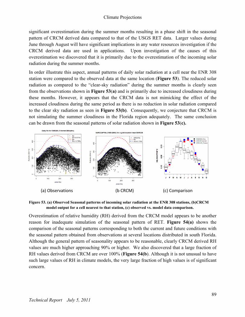
Climate Projections
89 Technical Report July 5, 2011
significant overestimation during the summer months resulting in a phase shift in the seasonal pattern of CRCM derived data compared to that of the USGS RET data. Larger values during June through August will have significant implications in any water resources investigation if the CRCM derived data are used in applications. Upon investigation of the causes of this overestimation we discovered that it is primarily due to the overestimation of the incoming solar radiation during the summer months.
In order illustrate this aspect, annual patterns of daily solar radiation at a cell near the ENR 308 station were compared to the observed data at the same location (Figure 53). The reduced solar radiation as compared to the “clear-sky radiation” during the summer months is clearly seen from the observations shown in Figure 53(a) and is primarily due to increased cloudiness during these months. However, it appears that the CRCM data is not mimicking the effect of the increased cloudiness during the same period as there is no reduction in solar radiation compared to the clear sky radiation as seen in Figure 53(b). Consequently, we conjecture that CRCM is not simulating the summer cloudiness in the Florida region adequately. The same conclusion can be drawn from the seasonal patterns of solar radiation shown in Figure 53(c).
(a) Observations (b CRCM) (c) Comparison
Figure 53. (a) Observed Seasonal patterns of incoming solar radiation at the ENR 308 stations, (b)CRCM model output for a cell nearest to that station, (c) observed vs. model data comparison.
Overestimation of relative humidity (RH) derived from the CRCM model appears to be another reason for inadequate simulation of the seasonal pattern of RET. Figure 54(a) shows the comparison of the seasonal patterns corresponding to both the current and future conditions with the seasonal pattern obtained from observations at several locations distributed in south Florida. Although the general pattern of seasonality appears to be reasonable, clearly CRCM derived RH values are much higher approaching 90% or higher. We also discovered that a large fraction of RH values derived from CRCM are over 100% (Figure 54(b). Although it is not unusual to have such large values of RH in climate models, the very large fraction of high values is of significant concern.

Trends in Climate and Sea Level Rise for South Florida
90 Technical Report July 5, 2011
(a) Seasonal pattern of Relative Humidity (b) Percent of RH > 1 in the CRCM data
Figure 54. Comparison of (a) simulated relative humidity from CRCM data with (b) observations at several locations in the south Florida. Also shown is the seasonal magnitudes of the percentage of RH values in the CRCM dataset which are greater than 100%.
Projections
In spite of the biases in temperature, precipitation and evapotranspiration data, it will be useful to understand the general trend and magnitude of the changes that could be expected during the 21st century using climate model data. CRCM data sets are available for both the 1970-2000 and 2040-2070 periods and they can be used compute the changes that could be expected during the middle of the 21st century (2050) compared to the base period of 1970-2000. Figure 55 shows the spatial maps of temperature changes predicted by CRCM circa 2050.
(a) Daily minimum (b) Daily maximum (c) Average
Figure 55. Change in temperature variables as predicted by CRCM circa 2050.
In general the change in all temperature variables (maximum, minimum, and average) appears to be about 2 °C overall. However, there is a markedly differing spatial pattern in each case. For example, in the case of minimum temperature, change appears to be lesser in the southeast part of the state. However, the expected increase in the maximum temperature appears to be large in the same region. It should be noted that the spatial difference in the change is small.

Climate Projections
91 Technical Report July 5, 2011
Figure 56 shows expected changes in precipitation (P) and reference grass evapotranspiration (RET) derived from the CRCM circa 2050. The expected precipitation change is positive or negative depending on the location. In the southeast the change is negative, indicating the annual precipitation by 2050 may be up to 2-3 inches lower compared to the base period of 1970-2000. North of Lake Okeechobee CRCM appears to predict a small increase in mean annual precipitation on the order of about 1-2 inches. In the case of RET, the increase across the entire state appears to be positive, on the order of 3-5 inches. Extreme values of larger changes appear to be concentrated at two locations (southwest and northeast) where anomalous results are suspected. Spatial patterns suggest that the increase in RET could be larger in the southern region. Comparison of precipitation suggests that the net change in P-RET could be significantly larger in the Everglades and the Lower East Coast region. As a consequence, water supply available for both human and natural systems could be less compared to the base period.
(a) Change in precipitation (b) Change in reference crop evapotranspiration
Figure 56. Change in precipitation and RET as predicted by CRCM circa 2050.
Summary
In this section we investigated the skills of General Circulation Models as well as statistically and dynamically downscaled regional models and their predictions. Grid resolution of most, if not all models, is inadequate to represent the Florida peninsula. The skill of mimicking local climatology of precipitation by GCMs is extremely poor. Seasonality of surface temperature is simulated by GCMs reasonably well but there are significant biases in individual models. In the case of statistically downscaled data, the simulations of climatology and the variability of temperature are adequate. This result is expected since bias correction methodology supports this outcome. Precipitation values, however, show some biases, particularly during the wet season.
The dynamically downscaled data (from CRCM belonging to the NARCCAP family) mimics the seasonal pattern of both temperature and precipitation reasonably well. However, there are spatial biases in the annual values in the range of 2 °C for temperature and -5 inches for precipitation. As with most downscaled applications (statistical and/or dynamical), spatial and

Trends in Climate and Sea Level Rise for South Florida
92 Technical Report July 5, 2011
temporal bias correction may be needed before NARCCAP model results are used for water resources investigations. In general, the use of NARCCAP (CRCM) model output variables to compute the potential evapotranspiration appears to be promising as it provides reasonable estimates of ET. However, there appear to be significant spatial and temporal biases. In particular, the ET appears to be overestimated during the summer months. This result is attributed largely to the overestimation of incoming solar radiation, possibly due to the lack of skill in the RCM to simulate cloud effect adequately. Another limitation was the overestimation of relative humidity (RH) as evidenced by the large percent of values above 100%. The underestimation of Reference ET during months outside the summer season is likely due to overestimation of RH. Again, other NARCCAP models need to be investigated to verify these general findings.
In spite of the limitations of the climate models, we chose to compute the projections circa 2050. A summary of these projections are shown in Table 20 below.
Table 20. Summary of median climate change for circa 2050.
Variable GCM (Figure 30) Statistically
Downscaled Data (Figure 42, 43)
Dynamically Downscaled Data
(Figure 55, 56) Average Temperature 1 to 1.5 ºC 1 to 2 ºC 1.8 to 2.1 ºC
Precipitation -10% to +10% -5% to +5% -3 to 2 inches Reference Crop Evapotranspiration
3 to 6 inches

Sea Level Rise and Extremes
93 Technical Report July 5, 2011
V. Sea Level Rise and Extremes
Introduction
Rising sea levels are a global reality. South Florida has received well deserved recognition as a critically sensitive region for both environmental (Senarath 2005, Kimball 2007) and societal concerns (Nicholls et al. 2008). From a socioeconomic perspective loss of habitable real estate and changes in civil support functions such as power, water, sewage and transportation are inevitable and must be considered in order to inform a portion of the decision-matrix used for urban adaptation strategies. Concerning water resources management, two primary concerns are saline contamination of coastal aquifers and wellfields, and reduction in coastal flood drainage capacity. Natural system impacts will also be significant, especially in the southern Everglades, Biscayne Bay and estuaries, where saltwater is displacing historically fresh water habitats and springs.
While most studies of sea level rise (SLR) are concerned with long term (decadal and centennial) changes in average sea level, another important aspect is the occurrence of low-probability, high-impact events such as storm surges and inland flooding from storms. These extreme events are recognized as a larger catalyst for societal change than long term changes in the environment (Bindoff et al., 2007). For example, recent work by Bender et al. (2010) strengthens evidence that climate change may decrease the total number of North Atlantic hurricanes, but increase the number of strongest (Saffir-Simpson scale 4 – 5) storms in the latter part of the 21st century. Regardless of future changes in storm frequency, as sea level continues to rise, storm surge events will produce increasingly severe impacts on coastal infrastructure and water resources (Mousavi et al., 2010).
A balanced view of potential changes should consider both long term and extreme event impacts based on well-informed decision support metrics developed by the scientific and analytical communities. The traditional design approach for projection of trends and extremes is to analyze historical data, in this case mean sea level and storm surges, and then apply regression curves or statistical likelihoods to the data in order to project these variables into the future. However, there are some limitations with this approach.
One problem is that historical data may not encompass enough samples of extreme events or may not have long-enough duration to adequately represent long-term trends. Even if the observations span centuries, questions of measurement biases and inaccuracies dominate data collected prior to the latter part of the twentieth century. Another issue is that many geophysical processes are statistically non-stationary, which simply means that the statistics change with time (they are not ‘stationary’). This is generally the case for climate variables. Thus, statistical averages, variances and regressions based on historic data may not represent future values of these variables.

Trends in Climate and Sea Level Rise for South Florida
94 Technical Report July 5, 2011
Yet another issue with traditional statistical forecasting based on observed data is the presence of teleconnections. Teleconnections represent the sensitive dependence on seemingly unrelated variables and are increasingly recognized as important drivers of natural systems. For example, Enfield et al. (2001) found a dependence between the Atlantic Multi-decadal Oscillation (AMO) and Lake Okeechobee inflows. Simply analyzing historic data without knowledge of these teleconnections could miss important system forcings and lead to erroneous projections. However, these feedbacks and links are not adequately represented in models and, coupled with our lack of comprehensive sampling and understanding of these processes, models are currently not mature enough to adequately represent these complex physical systems.
The foregoing realities illustrate why climate and sea level projections are highly variable and uncertain and why development of water management and societal adaptation strategies in response to sea level rise in south Florida poses significant challenges. Nonetheless, adaptation strategies require decision support analytics and one must proceed, based on available information and tools, to hopefully derive useful projections.
This chapter outlines the primary variables and issues associated with the projection of sea level rise and storm surge relevant to south Florida. We briefly review the components of sea level rise and historical sea level conditions and examine projections. We then explore issues associated with storm surge, identify teleconnections relevant to storm surge in Florida, and develop a method for probabilistic projection of storm surge levels as a function of the AMO. Finally, we examine implications of coastal flood control and aquifer contamination, and conclude by identifying directions for continued analysis of sea level rise in south Florida.
Sea Level Rise Components
Generally, three main contributors to sea level change are identified:
Steric - refers to the arrangement of atoms in space. In the context of SLR it pertains to the molecular expansion or contraction of water and aqueous ion species (salts) as a function of temperature and ionic concentrations. For example, as the heat content of the ocean increases the inter-molecular spacings in seawater also increase leading to a volumetric expansion and change in sea level.
Eustatic – represents changes in sea level due to water mass added or removed from the ocean. This component encapsulates a wide range of processes such as precipitation and continental runoff including glacial meltwater.
Isostatic – refers to changes in the elevation of the continental surface or ocean basins from tectonic or other geologic processes.
In relation to coastal planning and response, it is often convenient to consider the relative sea level rise which refers to the integrated effect of all three components rather than considering just the oceanic steric and eustatic components with respect to a geodetic datum. This relative sea
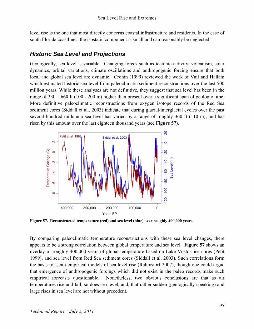
Sea Level Rise and Extremes
95 Technical Report July 5, 2011
level rise is the one that most directly concerns coastal infrastructure and residents. In the case of south Florida coastlines, the isostatic component is small and can reasonably be neglected.
Historic Sea Level and Projections
Geologically, sea level is variable. Changing forces such as tectonic activity, volcanism, solar dynamics, orbital variations, climate oscillations and anthropogenic forcing ensure that both local and global sea level are dynamic. Cronin (1999) reviewed the work of Vail and Hallam which estimated historic sea level from paleoclimatic sediment reconstructions over the last 500 million years. While these analyses are not definitive, they suggest that sea level has been in the range of 330 – 660 ft (100 - 200 m) higher than present over a significant span of geologic time. More definitive paleoclimatic reconstructions from oxygen isotope records of the Red Sea sediment cores (Siddall et al., 2003) indicate that during glacial/interglacial cycles over the past several hundred millennia sea level has varied by a range of roughly 360 ft (110 m), and has risen by this amount over the last eighteen thousand years (see Figure 57).
Figure 57. Reconstructed temperature (red) and sea level (blue) over roughly 400,000 years.
By comparing paleoclimatic temperature reconstructions with these sea level changes, there appears to be a strong correlation between global temperature and sea level. Figure 57 shows an overlay of roughly 400,000 years of global temperature based on Lake Vostok ice cores (Petit 1999), and sea level from Red Sea sediment cores (Siddall et al. 2003). Such correlations form the basis for semi-empirical models of sea level rise (Rahmstorf 2007), though one could argue that emergence of anthropogenic forcings which did not exist in the paleo records make such empirical forecasts questionable. Nonetheless, two obvious conclusions are that as air temperatures rise and fall, so does sea level; and, that rather sudden (geologically speaking) and large rises in sea level are not without precedent.

Trends in Climate and Sea Level Rise for South Florida
96 Technical Report July 5, 2011
IPCC Projections
Sea level projections from the United Nations Intergovernmental Panel on Climate Change (IPCC) are probably the most widely known (Bindoff et al., 2007). Projections from the IPCC Fourth Assessment Report (AR4) published in 2007 predicted that sea levels are likely to rise by 7.1 to 23.2 in (18 to 59 cm) over the period 1990-2100 (IPCC, 2007). This projection carefully considered available evidence, and based on climate model emission scenarios predicted a nonlinear acceleration of sea level over the 21st century. Figure 58 shows the IPCC AR4 projection for the A1B greenhouse gas emission scenario. One can clearly observe a sea level acceleration (sea level is not expected to rise at a linear, or constant rate, but will rise with a rate that becomes larger with time). However, concern that increased meltwater contributions from Greenland and Antarctica were not included in the projections, coupled with recent observations suggesting that sea level rise rates may already be approaching the higher end of the IPCC estimates (Rahmstorf et al. 2007, Jevrejeva et al. 2008) has led to a general consensus that the AR4 projections are too low. For example, subsequent to the IPCC projections, Rahmstorf (2007) developed a semi-empirical projection for sea level at 2100 (with respect to 1990) of 1.6 to 4.6 ft (0.5 to 1.4 m). The most recent investigations of ice-sheet melt have reconciled previously reported discrepancies, and Rignot et al. (2011) report: "The magnitude of the (ice-sheet melt) acceleration suggests that ice sheets will be the dominant contributors to sea level rise in forthcoming decades, and will likely exceed the IPCC projections for the contribution of ice sheets to sea level rise in the 21st century." Several other contemporary projections agree that glacial meltwater will increase levels and rates of SLR beyond IPCC AR4 projections; some of these are detailed in the following sections.
Figure 58. Time series of global mean sea level deviation from the1980-1999 mean. The grey shading shows the uncertainty in the estimated long-term rate of sea level change. The red line is a reconstruction of global mean sea level from tide gauges and the red shading denotes the range of variations from a smooth curve. The green line shows global mean sea level observed from satellite altimetry. The blue shading represents the range of model projections for the SRES A1B scenario for the 21st century, from Bindoff (2007).

Sea Level Rise and Extremes
97 Technical Report July 5, 2011
Government and Working Group Projections
At the national level, the National Science and Technology Council and U.S. Climate Change Science Program (USCCSP) submitted a report to the Environmental Protection Agency (EPA) recommending “Thoughtful precaution suggests that a global sea-level rise of 1 m (3.3 ft) to the year 2100 should be considered for future planning and policy discussions” (USCCSP 2009). However, it was noted that large uncertainties in the glacial meltwater contributions required further scientific scrutiny.
The United States Army Corps of Engineers (USACE) published guidance in July 2009 specifying a design procedure for coastal civil works projects (USACE, 2009). This method starts with a local SLR trend based on observed data to account for isostatic adjustments and local oceanographic conditions then adds a nonlinear time-dependent term to represent eustatic SLR contributions. The nonlinear (quadratic) term is modified from a National Research Council report (NRC, 1987) which assumed three scenarios corresponding to 1.6, 3.3 and 4.9 ft (0.5, 1.0 and 1.5 m) of eustatic SLR over the period 1987 – 2100. These scenarios are referred to as NRC I, NRC II and NRC III curves respectively, although in the USACE document the coefficients are adjusted to account for more recent global SLR estimates and the scenarios are referred to as ‘modified’ NRC curves. The USACE design method requires consideration of a baseline (historical trend extrapolation) and modified NRC I and NRC III curves representing a low, intermediate and high rate of SLR acceleration from eustatic contributions. To estimate the local historic SLR including the isostatic contribution, an average of SLR (NOAA 2009a) at five south Florida tidal stations (Miami Beach, Vaca Key, Key West, Fort Myers, Saint Petersburg) was computed providing a mean value of 2.37 mm/yr. Based on this average SLR, the current USACE method projections for south Florida starting in 2010 are shown in Figure 59.
At the regional governmental level, the Miami-Dade county Climate Change Task Force projected that “there is a very high likelihood that there will be at least a further 3-5 feet (0.9 – 1.5 m) of sea level rise during this century. This rise will most certainly continue at an accelerated rate into the following century” (Ruvin, 2008). Broward county adopted a sea level rise projection based on recommendation of their Climate Change Task Force which anticipates a rise from year 2000 of 10 - 20 inches (25 - 50 cm) by 2060, and 2 – 4 ft (61 - 122 cm) by 2100 (Broward, 2010). The South Florida Water Management District Interdepartmental Climate Change Group projected in 2009 that south Florida could expect 5 – 20 inches (13 - 25 cm) of sea level rise from 1990 through 2060 (SFWMD, 2009).
The Southeast Florida Regional Climate Change Compact (SFRCC) consisting of Monroe, Miami-Dade, Broward and Palm Beach counties is partnering with the South Florida Water Management District, Florida Atlantic University and U.S. Army Corps of Engineers to form a Technical Work Group tasked with development of a Unified Sea Level Rise Projection for Southeast Florida (SFRCC 2011) to inform and guide regional planning efforts with a consistent SLR projection. The SFRCC Work Group was committed to the goal of using science to inform

Trends in Climate and Sea Level Rise for South Florida
98 Technical Report July 5, 2011
Figure 59. South Florida sea level rise projections based on the USACE (2009) method.
policy, and through a series of facilitated panel discussions focusing on peer-reviewed scientific literature generally agreed that eustatic contributions from increased glacial meltwater will likely accelerate SLR over the coming century. After evaluating the most recent literature on SLR, and comparing several models of SLR with different acceleration scenarios, the Work Group recommended that U.S. Army Corps of Engineers’ method (USACE, 2009) be adopted as the unified southeast Florida projection. The projection uses Key West tidal data as a baseline rate with a reference date of 2010 for sea level equal to zero. Two key planning horizons were considered, 20 and 50 years, and the respective SLR projection ranges are 3 – 7 inches (7 – 18 cm) at 2030 and 9 – 24 inches (23 - 61 cm) at 2060. Due to the rapidly changing body of scientific literature on this topic, the Work Group recommended that the projection should be reviewed and possibly revised in two years (2012). It is difficult to graphically compare these projections since they are referenced to different start dates, therefore, a comparison is presented in Table 21.

Sea Level Rise and Extremes
99 Technical Report July 5, 2011
Table 21. Comparison of Different SLR Projections for South Florida.
Source Reference
Year SLR Projection (inches)
2030 2050 2060 2100 Historic South Florida Trend (2.37 mm/yr) 2000 2.8 4.7 5.6 9.3
Southeast Florida Regional Climate Change Compact (2011) 2010 3-7 9-24
Miami-Dade Climate Change Advisory Task Force (Miami-Dade County, 2008)
2000 >18 36-60
Broward County Climate Change Advisory Task Force (Broward County, 2010)
2000 3-9 10-20 24-48
South Florida Water Management District (SFWMD, 2009) 1990 5-20
Recent Scientific Literature Projections
Subsequent to the IPCC 2007 projections and the USACE guidance, the scientific community has continued to model and project sea level rise. Attention has focused on the glacial meltwater issue and in general, most contemporary projections are higher than the IPCC AR4 values. Table 22 lists projections at the year 2100 from recent peer-reviewed scientific publications indicating a movement towards increased acceleration of SLR and higher predictions than pre-2007 values.
Table 22. Sea level rise projections at 2100 from recent peer-reviewed scientific publications. [* Horton et al.: Both the IPCC AR4 and the semi-empirical sea level rise projections described here are likely to underestimate future sea level rise if recent trends in the polar regions accelerate.]
Author Min (ft) @ 2100
Max (ft) @ 2100
Jevrejeva et al., 2010 1.97 5.25 Grinsted et al., 2009 2.95 4.27 Siddall et al., 2009 0.23 2.69 Vermeera et al., 2009 2.46 6.23 Pfeffer et al., 2008 2.62 6.56 Horton et al., 2008 [*] 1.54 3.28
Acceleration
Given the observation that sea level change is variable with respect to time, and that the preponderance of evidence from recent ice loss and global climate models indicates that sea level rise is accelerating, one of the primary questions concerning projections is: what is the rate of change of sea level rise, i.e. what is the acceleration? The most comprehensive review of global accelerations was provided by Woodworth et al. (2009), wherein it is noted that analyses of accelerations over the late 19th and 20th centuries by several authors are in general agreement, and that climate teleconnections (PDO, NAO, AO and SOI) likely have a significant impact on the reported differences. The most geographically comprehensive quantification was reported by
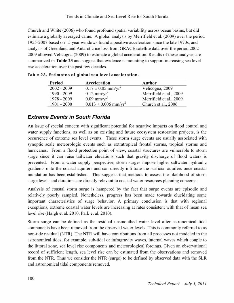
Trends in Climate and Sea Level Rise for South Florida
100 Technical Report July 5, 2011
Church and White (2006) who found profound spatial variability across ocean basins, but did estimate a globally averaged value. A global analysis by Merrifield et al. (2009) over the period 1955-2007 based on 15 year windows found a positive acceleration since the late 1970s, and analysis of Greenland and Antarctic ice loss from GRACE satellite data over the period 2002-2009 allowed Velicogna (2009) to estimate a global acceleration. Results of these analyses are summarized in Table 23 and suggest that evidence is mounting to support increasing sea level rise acceleration over the past few decades.
Table 23. Estimates of global sea level acceleration.
Period Acceleration Author 2002 - 2009 0.17 ± 0.05 mm/yr2 Velicogna, 2009 1990 - 2009 0.12 mm/yr2 Merrifield et al., 2009 1978 - 2009 0.09 mm/yr2 Merrifield et al., 2009 1901 - 2000 0.013 ± 0.006 mm/yr2 Church et al., 2006
Extreme Events in South Florida
An issue of special concern with significant potential for negative impacts on flood control and water supply functions, as well as on existing and future ecosystem restoration projects, is the occurrence of extreme sea level events. These storm surge events are usually associated with synoptic scale meteorologic events such as extratropical frontal storms, tropical storms and hurricanes. From a flood protection point of view, coastal structures are vulnerable to storm surge since it can raise tailwater elevations such that gravity discharge of flood waters is prevented. From a water supply perspective, storm surges impose higher saltwater hydraulic gradients onto the coastal aquifers and can directly infiltrate the surficial aquifers once coastal inundation has been established. This suggests that methods to assess the likelihood of storm surge levels and durations are directly relevant to coastal water resources planning concerns.
Analysis of coastal storm surge is hampered by the fact that surge events are episodic and relatively poorly sampled. Nonetheless, progress has been made towards elucidating some important characteristics of surge behavior. A primary conclusion is that with regional exceptions, extreme coastal water levels are increasing at rates consistent with that of mean sea level rise (Haigh et al. 2010, Park et al. 2010).
Storm surge can be defined as the residual unsmoothed water level after astronomical tidal components have been removed from the observed water levels. This is commonly referred to as non-tide residual (NTR). The NTR will have contributions from all processes not modeled in the astronomical tides, for example, sub-tidal or infragravity waves, internal waves which couple to the littoral zone, sea level rise components and meteorological forcings. Given an observational record of sufficient length, sea level rise can be estimated from the observations and removed from the NTR. Thus we consider the NTR (surge) to be defined by observed data with the SLR and astronomical tidal components removed.

Sea Level Rise and Extremes
101 Technical Report July 5, 2011
The tidal observations and astronomical predictions used to compute NTRs were obtained from hourly NOAA (2009) tide gauge records at Key West (1913-2008), Pensacola (1923-2008) and Mayport (1928-2008), Florida. The hourly data were detrended according to sea level rise trends computed at each station by NOAA (2009a). We then compute hourly NTR by subtracting the prediction from the observed data, and finally compute monthly block-maxima (the maximum NTR from non-overlapping time windows of duration one month) from the hourly NTR. Figure 60 plots the NTR monthly block-maxima of the stations. Each of the ‘spikes’ records a significant event where coastal sea level was higher than normal. A comparison of these time series with recorded hurricane and tropical storm landfalls correlates well.
Figure 60. Non-tide Residual (NTR) monthly block-maxima at Key West, Pensacola and Mayport Florida.
By their nature, extreme events such as storm surges are difficult to predict. Traditionally, one turns to statistics of historical events and estimates exceedance distributions in terms of the event return period. A familiar example is the 100-year flood level considered in civil infrastructure design. As observation, modeling and understanding of climate processes advances, we may be able to use newly discovered relationships between climate indices and hydrological forcings.
The next section explores such a link between the Atlantic Multi-decadal Oscillation (AMO) and storm surge in Florida.

Trends in Climate and Sea Level Rise for South Florida
102 Technical Report July 5, 2011
Climate Links to Extreme Events
When viewed from the perspective of regional climate indices, several researchers have identified plausible links to storm surge (Woodworth et al. 2009, Woodworth and Blackman 2004, Bromirski et al. 2003, Woodworth and Blackman 2002, Zhang et al. 2000a). Seymour found that an El-Niño Southern Oscillation index displayed useful skill in the prediction of southern California severe coastal wave events (Seymour 1996), and it has been shown that the AMO has significant influence on the climate and associated hydrology of the United States and Lake Okeechobee (Trimble et al. 2006, Enfield et al. 2001). The AMO is related to the size of the Atlantic Warm Pool (AWP) (Enfield and Cid-Serrano, 2010). In addition, large AWP’s result in weakened tropospheric vertical wind shear and a deep warm upper ocean and increased Atlantic hurricane activity (Wang et al., 2006). One can therefore suggest a link between the AMO/AWP and increased storm activity as a forcing mechanism and Florida storm surge levels as a response.
A linkage of extreme sea levels to natural phenomena such as the AMO may allow planners to anticipate some of the variability of storm impacts on a decadal or multidecadal scale. Although deterministic prediction of the AMO is not possible at this time, the expectation is that such predictions coupled with statistics of extreme events may provide decision-support for coastal planners concerned with infrastructure improvements and policy decisions. A probabilistic framework for this endeavor is discussed in the following section. Here we provide evidence for a causal link between extreme coastal water levels and duration at Key West and Pensacola with the AMO.
AMO Relation to Florida Storm Surge
In this analysis, we use the hourly NTR (surge) data and compute a 3-day moving sample standard deviation (σ) on the NTR. To clearly identify extreme events based on their deviation (energy) above background water level (tidal) oscillations, we apply a minimum threshold (σmin) to the NTR deviation and record corresponding events for which σ > σmin. Values of σmin were selected as the 99.5% percentile value of NTR deviation computed from an empirical cumulative distribution function. We also require each event to have a minimum duration of 3 hours.
Linear Regressions
Figure 61 (a) plots the event water levels (surge height), (b) the associated NTR deviation and (c) the event duration from Key West. The unsmoothed AMO index is shown in gray. Since several studies have indicated positive links between regional climate indices and extreme water levels (Woodworth and Blackman 2004, Bromirski et al. 2003, Woodworth and Blackman 2002) we also assess linear regressions between surge events and the AMO index (Figure 61 d, e, f).

Sea Level Rise and Extremes
103 Technical Report July 5, 2011
Figure 61. Key West NTR (surge) data and linear regressions (dashed black line) with 95% confidence limits (dashed red lines). p-values to 4 decimal places are shown for each variable. a) Water level vs. Year b) NTR deviation vs. Year c) NTR duration vs. Year d) Water level vs. AMO e) NTR deviation vs. AMO f) NTR duration vs. AMO.
Linear regression of surge event variables against time (Figure 61 a) finds a positive trend of surge water level at Key West of 2.9 mm/yr ± 1.0, consistent with NOAA estimates of mean sea-level rise (NOAA MSL) and reinforcing the findings of others that secular increases in storm surge heights are due to sea level rise. The surge deviation (Figure 61 b) and duration (Figure 61 c) exhibit no linear relation as a function of time. The p-values indicate that the linear trend in water level is not an artifact of the data (at the 1 – 0.0041 = 99.9959% confidence level), while the deviation and duration values indicate no valid linear dependence.
Considering the AMO dependence (Figure 61 d, e, f), a weak relationship is shown for all three surge variables (height, deviation, duration), while the p-values indicate rejection of the non-trend hypothesis at significance levels of 100% (surge level), 95.0% (deviation) and 99.7% (duration). These linear model results indicate that at Key West there is a dependence of surge on AMO, with a very high likelihood that the dependencies are real and not artifacts of the data. The fact that the dependencies are weak indicates that the linear models are insufficient to properly account for the surge variance as a function of AMO. Surge values and linear models versus time at Pensacola are plotted in Figure 62 (a, b, c), while Figure 62 (d, e, f) plots surge event regressions against AMO. Similar to the Key West results, the data suggest trends significant at the 95% confidence level for all three event variables as a function of AMO.
d)
e)
f)

Trends in Climate and Sea Level Rise for South Florida
104 Technical Report July 5, 2011
Figure 62. Pensacola NTR (surge) data and linear regressions (dashed black line) with 95% confidence limits (dashed red lines). p-values to 4 decimal places are shown for each variable. a) Water level vs. Year b) NTR deviation vs. Year c) NTR duration vs. Year d) Water level vs. AMO e) NTR deviation vs. AMO f) NTR duration vs. AMO.
To summarize these findings, regression fit parameters for surge events against AMO are shown in Table 24. As evidenced by the low correlation coefficients a linear model cannot adequately represent the surge variance and will therefore have no utility for accurate event prediction. Nonetheless, the low p-values suggest that the trends are significant (they are not from random realizations of data artifacts) and thus the weak linear dependencies may provide a coarse demarcation for assessing event behavior as a function of AMO. For example, at Key West the trend in duration is estimated at 38.3 hr/AMO. If the AMO is expected to shift from a cool phase with an index value of -0.3 to a warm condition with a value of 0.3, an increase in expected event duration of about 23 hours could be anticipated. Likewise, surge water level changes over the same AMO conditions would correspond to a rise of roughly 1 ft (0.31 m).
Table 24. Linear regression parameters of surge with respect to AMO.
p-value fit coefficient r2 Key West Water Level 2.61E-05 0.522 ± 0.114 0.265 Deviation 0.050 0.040 ± 0.020 0.064 Duration 0.003 38.26 ± 12.50 0.139 Pensacola Water Level 0.003 0.777 ± 0.252 0.123 Deviation 0.043 0.094 ± 0.045 0.059 Duration 0.016 34.11 ± 13.82 0.082
d)
e)
f)

Sea Level Rise and Extremes
105 Technical Report July 5, 2011
Mean Event Statistics
Linear regressions against AMO suggest positive trends in the event variables as AMO transitions from cool (negative) to warm (positive). To provide a quantitative assessment of expected event variables as a function of AMO conditions, one can partition the AMO into cool and warm regimes. We define an AMO cool phase with values of AMO < -0.1, an AMO warm phase as AMO > 0.1. With this partition of AMO, mean values of event variables are presented in Table 25 where we see an interesting commonality amongst the three stations, there is a mean increase for all three event variables with respect to warm AMO conditions suggesting that statistics relevant to coastal response planning could be applied. For example, during an AMO warm-phase one might expect a mean-increased event duration of 17 hours at Key West in relation to a cool-phase event, and at Pensacola an average increase of water level by 0.28 m (0.92 ft).
Table 25. Mean event statistics as a function of AMO partition. N is the number of events.
AMO Duration
(hr) Water Level (m) NAVD
Deviation (m) N
Key West cool 23.4 -0.090 0.120 23 warm 40.7 0.188 0.140 18 Pensacola cool 26.8 0.392 0.250 19 warm 39.6 0.668 0.283 30
Temporal Dependence of Storm Surge on AMO
In south Florida it is known that sea level and coastal aquifer groundwater levels are coherently linked (Park and Richardson, 2006), and that sea level rise promotes saltwater intrusion into the surficial aquifer (Parker et al., 1955). The spatiotemporal intrusion of saltwater is dependent on the level and duration of the sea level rise or storm surge event, as well as the hydraulic conductivity of the aquifer. Therefore, understanding the temporal characteristics of extreme sea level events has relevance to coastal water resources interests.
The preceding section shows that surge water level and duration at Key West and Pensacola have statistically significant trends when regressed against the AMO index. Surge events during AMO warm conditions are associated with longer durations having a mean increase in duration of approximately 17 hours at Key West and 13 hours at Pensacola. To examine characteristics of these temporal shifts a frequency analysis is warranted; however, owing to the transient nature of these events a Fourier decomposition may poorly represent the event power as a function of frequency. A better tool for transient analysis is the wavelet transform. A timeseries analysis based on the Maximal Overlap Discrete Wavelet Transform (MODWT) (Percival and Walden, 2006) applied to surge events is used to decompose event energy into independent components. Comparison of energy partitions as a function of the AMO regime can then be assessed.

Trends in Climate and Sea Level Rise for South Florida
106 Technical Report July 5, 2011
Briefly, the MODWT decomposes an input time series vector X of length N into a set of additive components, each of which captures temporal variations at different timescales:
J
J
j
j SDX (8)
where the index j represents a distinct wavelet level. The Dj are referred to as wavelet details, and SJ the smooth, each a vector of length N. The details capture transient and oscillatory behavior at different time scales; the smooth corresponds to a moving average of the signal. Note that there are a total of J+1 levels (J details and one smooth) so that by convention a 7-level MODWT actually has 8 components. Each wavelet level is computed with a matrix transform
jjj W ΦD T and JJJ V ΨS T where W and V are N x N matrices of MODWT coefficients, Φ
and Ψ are referred to as the wavelet coefficient and scaling coefficient vectors respectively. The wavelet and scaling coefficients are the result of cascaded high-pass wavelet filters (h)
recursively applied to the input: Nmod,1
1
0,, X
t
L
lljtj
j
h , or a low-pass scaling filter (g):
Nmod,1
1
0,, X
t
L
lljtj
j
g where the filter width at each level Lj = (2j - 1)(L - 1) + 1 is determined by
the length of the mother wavelet filter L. In terms of the MODWT matrix and wavelet\scaling coefficients the input can then be represented as:
JJj
J
jj VW ΨΦX TT . (9)
The MODWT provides a convenient encapsulation of the signal energy in terms of the wavelet and scaling coefficient vectors:
222 |||||||||||| J
J
jj ΨΦX (10)
which are related to the sample variance of X (Percival and Walden, 2006). Preservation of the total variance is an important feature of the MODWT, one which we exploit to examine energy conservative changes in extreme event behavior under changing climatic conditions.
Wavelet processing is performed with the wavelets package of the R statistical computing suite of programs (R Foundation, 2008). We employ a seven level (J=7) wavelet transform based on the least asymmetric mother wavelet, maximum temporal scales for the wavelet levels (W1 – W7), and minimum temporal scale for the scaling level V7 are listed in Table 26.
Table 26. Maximum temporal scale of each wavelet level (W1 – W7), and minimum temporal scale of the scaling level V7.
Level W1 W2 W3 W4 W5 W6 W7 V7 Scale (hr) 4 11 25 53 109 221 445 381

Sea Level Rise and Extremes
107 Technical Report July 5, 2011
To ensure that end-effects of wavelet periodicity are avoided, all event datasets were of length 1335 hours, three times the length of the longest wavelet scale (445), with the event centered in the record
Surge Event Energy Partitions
To quantify surge temporal energy characteristics we specify a metric of the relative contribution of the jth wavelet level to the total energy at any point in time t:
|)(|
|)(|)(e
t
tt J
jj
jj
Φ
Φ. (11)
Since extreme sea level events do not occur at a single point in time, but span a finite duration, a more comprehensive metric considers the relative event energies over the event duration. Event durations, τ, were defined by Park et al. (2010) as the contiguous interval over which the moving sample variance of the NTR exceeded the 99.5 percentile.
With this extension we define the relative event energy of the jth wavelet level as:
J
jjjj dttdtt |)(||)(|E ΦΦ . (12)
Owing to the energy conservative nature of the wavelet coefficients as evidenced in Equation
10, the relative ratios expressed in ej and Ej are also energy conservative, i.e. J
jj
J
jj 1Ee .
Another metric of interest is the active interval, Tj, of each wavelet level surrounding the peak energy of the event. This provides information about the temporal contribution of energy to the event across the wavelet scales. We employ a derivative search algorithm to estimate Tj (Park et al., 2010).
The energy and duration statistics were computed on the Key West and Pensacola storm surge data resulting in eight values of Ej and Tj for each event. The events are then partitioned into two subsets based on the value of the AMO index during the event (warm or cool as previously defined). Mean values of relative energy and interval are computed for each AMO index subset, with results for Key West presented in Table 27. Also shown in Table 27 is the change in fractional energy from AMO cool to warm conditions, ΔĒj, and estimates for a one-sided 90% confidence bound on the change.
Considering the energy change ΔĒj in detail, we see that the largest change (~7%) was a loss of energy from the long period smooth V7 when conditions changed from AMO cool to AMO warm. That there is a shift of energy into the dynamic timescales (non-moving average) is consistent with previous findings of increased extreme water level event variability during AMO warm phases (Park et al., 2010).

Trends in Climate and Sea Level Rise for South Florida
108 Technical Report July 5, 2011
The next most significant change is the addition of nearly 3% of event energy in the W5 level under AMO warm conditions, followed by roughly 1.5% increases in the W6 and W7 levels. The other short timescales W1, W2 and W4 exhibit small increases, while the sub-diurnal W3 scale has a 1% loss. Overall, the data suggests that extreme event variability at Key West increases at
Table 27. NTR event relative energy and temporal periods at Key West.
Wavelet Level
Ēj AMO cool
Ēj AMO warm
ΔĒj
90% ΔĒj
Tj (hr) AMO cool
Tj (hr) AMO warm
W1 0.0184 0.0245 0.0061 0.0008 2.8 3.8 W2 0.0274 0.0309 0.0034 0.0012 5.9 6.3 W3 0.0610 0.0508 -0.0103 0.0025 10.9 10.9 W4 0.0626 0.0738 0.0113 0.0016 19.3 24.7 W5 0.0898 0.1185 0.0287 0.0026 38.4 36.6 W6 0.1557 0.1726 0.0168 0.0048 78.3 93.7 W7 0.1449 0.1607 0.0158 0.0046 153.6 156.4 V7 0.4402 0.3683 -0.0719 0.0098 340.3 312.1
dynamic timescales between 20 and 150 hours during AMO warm conditions with the largest increase at roughly a 37 hour period. This increase may be a reflection of increased storm activity supported by a larger ocean thermal reservoir.
Results for the Pensacola station are shown in Table 28. In this data we see that there is little redistribution of event energy at timescales shorter than the W4 (daily) level. Even at the 45 hour period of W5 there is a less than 1% increase during AMO warm conditions. It is known that the extensively shallow bathymetry offshore Pensacola significantly modifies the amplitude and phase response of storm surges (Harris 1963). This suggests that event energy changes at timescales less than one day can be suppressed by bathymetry controlled boundary conditions and bottom friction, consistent with historical surge behavior. Regarding the longer timescales there is a small shift of energy out of the dynamic levels W6 and W7, and into the long-term average scale V7.
Table 28. NTR event energy and temporal periods at Pensacola.
Wavelet Level
Ēj AMO cool
Ēj AMO warm
ΔĒj
90% ΔĒj
Tj (hr) AMO cool
Tj (hr) AMO warm
W1 0.0186 0.0141 -0.0045 0.0004 3.2 2.9 W2 0.0161 0.0155 -0.0005 0.0003 5.0 5.4 W3 0.0306 0.0302 -0.0003 0.0006 11.8 12.4 W4 0.0708 0.0738 0.0029 0.0014 23.0 24.3 W5 0.1182 0.1267 0.0085 0.0021 44.7 46.5 W6 0.2178 0.2054 -0.0123 0.0038 95.1 88.6 W7 0.2279 0.2036 -0.0243 0.0030 165.4 170.1 V7 0.3001 0.3307 0.0306 0.0037 272.5 275.9

Sea Level Rise and Extremes
109 Technical Report July 5, 2011
Results of Temporal Surge Analysis
The analysis constructs an energy conservative metric which facilitates comparison of the relative energy of extreme events across temporal scales. Application of the metric to subsets of event data as a function of the AMO suggests a redistribution of energy in temporal bands in response to regional climate conditions. In the case of surge events at Key West the analysis finds that under AMO warm conditions the average increase in event variability is primarily at temporal scales from 20 to 150 hours (roughly 1 to 6 days) with the most significant increase of approximately 3% near a 37-hour period. We hypothesize that the redistribution of event energy into these dynamic timescales reflects an increase in storm energetics as a result of an increase in ocean heat content as reflected by the AWP (Enfield et al. 2010, Wang et al. 2006). Results at Pensacola detected a weaker redistribution of mean event energy with no significant changes at timescales below 45 hours.
The results show that surge events detected from coastal tidal records can temporally resolve exchanges of energy between temporal bands as a function of a regional climate index. This provides an approach that may eventually be applied to correlate temporally dependent geophysical responses with regional climate forcings. If it becomes possible to forecast these climate indices, then such links may provide useful decision support information. For example, in the case of coastal stations where saltwater intrusion forced by extreme events is a concern, the temporal statistics could provide input to hydrological models used to estimate the spatiotemporal influence of the intrusion. Another concern is the reduction of coastal flood control release capacity as mean sea level rise and extremes occur. Statistical expectation of the temporal span over which the extreme levels will persist based on climate outlooks may allow the development of appropriate flood control routing and adaptation strategies.
Analysis
This analysis finds that during AMO warm phases that storm surge levels and duration are expected to be higher than during AMO cool conditions, exacerbating the difficulties of discharging flood waters from urbanized areas during storm events. Since the AMO switches from cold to warm phases over multidecadal scales with no fixed periodicity, forecasting the index is currently problematic. However, there has been progress in the formulation of an empirical probabilistic framework for AMO phase changes (Enfield and Cid-Serrano, 2006). The application of such models with AMO-related statistics as presented here can provide decision support for infrastructure design and management policies and decisions. How to approach such a climate-dependent projection is discussed in the following section.
Projection of Extreme Events
That there is a dependence between Florida surge levels and the AMO suggests that information regarding the current or forecast state of the AMO might be leveraged to refine predictions of surge levels. Such information does not currently exist in terms of model forecasting, however,

Trends in Climate and Sea Level Rise for South Florida
110 Technical Report July 5, 2011
Enfield and Cid-Serrano (2006) have developed a probabilistic framework to assess AMO phase changes. This opens the possibility that water managers may be able to incorporate climate-dependent scenarios in the development of management strategies aimed at extreme event mitigation.
A goal of this section is to quantify probabilistic surge return levels and periods based on historical tide gauge data at Key West, Pensacola and Mayport. We then turn to the projection of surge levels based on SLR scenarios currently required by the U.S. Army Corps of Engineers in the design of coastal projects (USACE 2009). Based on evidence that extreme coastal water levels are increasing at rates consistent with that of mean sea level rise, the SLR scenarios are used as location parameters to probability distributions of observed storm surges allowing estimation of future surge return statistics. Next, the dependence of storm surge on the AMO is coupled with the probabilistic AMO transition framework suggested by Enfield and Cid-Serrano (2006) in order to project surge return levels as a function of pre-existing and forecast AMO conditions. Lastly, the projected surge values are examined in the context of design information for south Florida water management adaptation strategies.
Historical Storm Surge Distributions
NTR levels can be associated with expected return periods by equating the probability of exceedance of the NTR with the inverse of a return period, that is, the return level is the quantile of the fitted probability distribution corresponding to the upper tail probability 1/(T NT), where T is the return period and NT the number of data points per period. In the present analysis we use a return period of one year and monthly block-maxima so that NT = 12. The distribution model we employ is the generalized extreme value (GEV) (Coles, 2001) which has a distribution function
/1
1exp)(x
xF (13)
where ε, σ and μ are the shape, scale and location parameters, respectively. Maximum likelihood fits of the GEV were performed on the NTR data of Figure 60 with the R (R Development Core Team 2008) evd package (Stephenson, 2009). The corresponding NTR return levels are shown in Figure 63. These distributions estimate the expected frequency of occurrence of NTR levels, and, as expected from inspection of the data in Figure 63 return levels at Pensacola and Mayport are roughly twice those of Key West. Curves of this type based on observed data are conventionally considered as design criteria in the development of coastal infrastructure. In a world of stationary sea level statistics, this could be a viable approach, however, in light of the inherent non-stationarity of SLR and extremes, consideration should be given to statistics based on SLR projections which incorporate changing climate.

Sea Level Rise and Extremes
111 Technical Report July 5, 2011
Figure 63. NTR (storm surge) return levels estimated from GEV fits to the NTR data in Figure 57. 95% confidence intervals are shown with the dotted lines.
To examine the AMO dependence we partition the NTR data at Key West and Pensacola into two AMO regimes referred to as Warm (values of the index greater than 0.1) and Cool (values less than -0.1). With GEV distributions fit to these two subsets the resulting return levels are depicted in Figure 64. Here we see a statistically significant decomposition of the Pensacola
Figure 64. NTR (storm surge) return levels at Key West and Pensacola as a function of two AMO index regimes: Warm (index > 0.1) and Cool (index < -0.1). Dotted lines are 95% confidence levels.
return levels as a function of the AMO index at the 95% confidence level, while the Key West estimates have a slight overlap but still suggest AMO dependent NTR behavior. The implication is that warm AMO conditions are associated with increased NTR levels as a function of return

Trends in Climate and Sea Level Rise for South Florida
112 Technical Report July 5, 2011
period. This is hypothesized to represent a link between the AMO and size of the Atlantic Warm Pool (Enfield and Cid-Serrano, 2010), facilitating increased tropical storm activity (Wang et al. 2008, Goldenberg et al. 2001) and resulting in more likely extreme coastal water levels.
Surge Projections
As discussed earlier, there is ample evidence that secular trends in coastal surge are driven primarily by the change in mean SLR. It is then plausible to transfer projections of SLR onto the NTR distributions for estimates of future NTR behavior. While this is straightforward, a joint probability formalism with probabilistic convolution is required to account for transference of the SLR uncertainty to the projected NTR statistics (Liu et al. 2010, Hunter 2010). Here we do not attempt to account for the uncertainty in the SLR projections, although work is currently in progress to address this issue. Here we will adopt projections proposed by the U.S. Army Corps of Engineers (USACE) for the design of civil infrastructure impacted by SLR (USACE, 2009). Figure 59 plots these SLR projections for south Florida.
A surge projection is estimated by applying a SLR scenario (NRC I or NRC III) as a time-dependent location parameter to an NTR GEV fit to historic data (return levels of the GEV’s are shown in Figure 64). Projected GEV distribution of the NTR at time t can then be modeled as:
/1)(
1exp),(tRNTR
tNTRF (14)
where R(t) is the SLR projection at time t. It should be noted that these projections implicitly include a SLR component with R(t), but not an astronomical component as it was removed by definition of the NTR. A geodetic referenced total water level projection would require addition of predicted astronomical tide to the NTR projection.
Projected NTR return levels at Key West with the modified NRC I scenario are shown in Figure 65, and with NRC III values in Figure 66. The horizontal axis corresponds to the future time t of Equation 14 in years, and the vertical axis to the NTR return period in years.
Both of these scenarios suggest significant changes in NTR behavior over the coming decades. Considering the NRC I scenario depicted in Figure 65, at a future time of 5 years the NTR return level of 0.5 m has a return period of approximately 30 years, while at a future time of 25 years, the 0.5 m NTR level has a return period of roughly 8 years. The NRC III scenario at Key West suggests a more aggressive situation with 0.5 m NTR levels predicted every couple of years at a future time of 20 years.

Sea Level Rise and Extremes
113 Technical Report July 5, 2011
Figure 65. Projected NTR return levels at Key West based on a time-dependent SLR specified by the modified NRC I curve.
Figure 66. Projected NTR return levels at Key West based on a time-dependent SLR specified by the modified NRC III curve.
Such an acceleration of surge levels warrants closer scrutiny. A comparison of projected NTR return levels under NRC I and NRC III scenarios at 50 years with historical return levels (Table 29) shows that if historic conditions prevail, such that eustatic SLR components remain linear, then expected NTR return levels at a 50-year return period at Key West are within about (0.52 – 0.38) = 0.14 m of values with 5-year return period. At Pensacola and Mayport the difference is roughly 0.3 m. However, under conditions projected by NRC I or NRC III scenarios there is a significant increase in expected NTR levels at all return periods. For example, at Key West under

Trends in Climate and Sea Level Rise for South Florida
114 Technical Report July 5, 2011
Table 29. Comparison of historical NTR return levels (m) with projections at 50 years in the future (2060) based on NRC I and NRC III SLR scenarios.
Key West Pensacola Mayport Return
Period (yrs) Historic NRC I NRC III Historic NRC I NRC III Historic NRC I NRC III
5 0.38 0.62 0.99 0.78 1.01 1.39 0.83 1.07 1.45 10 0.43 0.66 1.04 0.88 1.11 1.49 0.92 1.15 1.53 20 0.47 0.70 1.08 0.99 1.22 1.60 1.00 1.23 1.61 30 0.49 0.72 1.10 1.05 1.28 1.66 1.04 1.28 1.65 40 0.51 0.74 1.12 1.10 1.33 1.71 1.08 1.31 1.69 50 0.52 0.76 1.13 1.13 1.37 1.74 1.10 1.34 1.71
NRC I conditions the NTR return levels at a 5-year return period is 0.62 m, which is larger than the return level under historic conditions at a 50-year return period (0.52 m). This predicts that under NRC I conditions within a 5-year period an NTR event will exceed that of a one-in-fifty year event under historic conditions. At Pensacola and Mayport, the NRC I projection at a 10 year return period roughly equates to that of the historic levels at a 50-year return period.
Effectively, these projections suggest that a given expected surge return level is being ‘condensed’ in time by SLR such that the interval between surge occurrences can rapidly decrease. Considering that both Key West and Pensacola are low elevation areas, such an increase in NTR levels has potential to create significant negative impacts.
AMO Dependence
As discussed earlier, there is a body of evidence establishing a dependence between the AMO index and NTR levels and durations at Key West and Pensacola. Enfield and Cid-Serrano (2006) developed a probabilistic interpretation of AMO phase-change that can provide a basis for projection of AMO-dependent climate responses towards the goal of informing risk-based decision support. Here we attempt such a synthesis by combining AMO phase-transition statistics with AMO-dependent GEV distributions of NTR at Key West.
Enfield and Cid-Serrano (2006) analyzed an AMO index developed from instrumental and tree-ring reconstruction records spanning a 424-year period. Based on a resampling scheme they fit a gamma distribution to phase changes of the reconstruction and developed a probabilistic projection for AMO phase changes. Figure 67 plots projections from equation 1 of Enfield and Cid-Serrano (2006) estimating probabilities for AMO phase changes based on the number of years since the last transition and the number of years into the future for which a probabilistic assessment of phase change is desired. For example, if it has been 5 years since the last AMO regime change, then at 15 years in the future the probability of an AMO regime change during the 15-year period is approximately 60%. With a method to estimate future AMO phase shifts, our attention turns to joining AMO-dependent NTR statistics with AMO phase change projections. With the assumption that we will model only one AMO transition, and that the AMO states are restricted to a binary regime of either warm or cool (as defined earlier), we can

Sea Level Rise and Extremes
115 Technical Report July 5, 2011
Figure 67. Probabilistic assessments for an AMO phase shift based on the number of years from the last shift and the number of years into the future. Computed from equation 1 of Enfield and Cid-Serrano (2006).
denote the probability of changing from the current phase to the other within the forecast time period as p, and the probability of remaining in the same phase as 1 – p. Assuming independence between AMO regime changes, the distribution function for NTR levels as a function of forecast period t can be specified as:
),(1),(),( tNTRFptNTRFptNTRF CN (15)
where FC corresponds to the projected NTR GEV distribution function of the current AMO phase and FN the next regime.
As an example of AMO-dependent NTR projections we evaluate return levels computed from GEV distributions for Key West and Pensacola at future times of 15 and 25 years (calendar years 2025 and 2035) for the modified NRC III SLR projections. Values of p are estimated from the projections of Enfield and Cid-Serrano (2006) with previous AMO regime shifts at 5 and 20 years past. Figure 68 plots the resulting AMO-dependent NTR projections for Key West where the NTR distributions are denoted by the pair: [Initial AMO regime, Years since last AMO shift]. For example, the curve labeled “Cool 20” in panel a) has the initial (current) distribution FC assigned to the Key West AMO cool regime GEV projected at 15 years in the future (2025) based on modified NRC III SLR, while the AMO transition probability p was selected for the previous AMO shift having occurred 20 years in the past. Also shown in Figure 68 are the NTR return levels fit to the observed data (Figure 60) and return levels for the modified NRC III SLR projections without regard for AMO dependence (vertical sections of Figure 68 at years 2025 in panel a, and 2035 in panel b).

Trends in Climate and Sea Level Rise for South Florida
116 Technical Report July 5, 2011
Figure 68. Key West NTR return level projections based on synthesis of AMO warm and cool NTR distributions according to equation 3 based on modified NRC III SLR projections. The AMO phase change probability is computed for a future time of 15 or 25 years (2025 or 2035). Curves are denoted according to the initial AMO phase of warm or cool, and the previous AMO shift at either 5 or 20 years ago. Return levels are also shown for the historic data, and for the modified NRC III projection without AMO dependence. a) AMO-dependent projections at 15 years (2025), b) AMO-dependent projections at 25 years (2035).
Aside from the expected increase in NTR return levels due to the modified NRC III sea level projections, several things are apparent in Figure 68. First, for the projections of 15 years (2025) in panel a, there is not a great deal of dependence on the AMO conditions. While the results suggest that transitioning from a currently cool AMO regime into a warm one can produce expected NTR events with higher amplitudes than a transition from currently warm to cool, the amplitude of the change is small, roughly 0.1 m. However, when considering a 25-year projection (panel b), the AMO-dependence becomes clearer, again showing that a transition from cool to warm conditions portends higher NTR event levels. The change in AMO-dependence between the 15 and 25 year projections can partially be explained by the differences in AMO transition probabilities. For the 25-year future projection, AMO transition probabilities are above 80% regardless of the time since the last transition, and near 100% when the previous transition was more than 10 years past (Figure 67). In such cases we expect the AMO-dependence exhibited in Figure 68 to contribute to a large degree, whereas for cases when the AMO

Sea Level Rise and Extremes
117 Technical Report July 5, 2011
transition probabilities are smaller, as with the 15-year projection, the AMO-dependence will be mitigated.
Another conclusion supported by Figure 68 is that at Key West the length of time since the last AMO transition is less important than the current and future state of the AMO. Generally, when the current state is AMO cool, and there will be a transition into AMO warm, one can expect higher amplitude NTR events.
It must be mentioned that we have assumed only a single AMO transition will occur. When dealing with 25-year forecasts, especially when the previous AMO transition has occurred more than a few years in the past, it is entirely possible, as demonstrated in reconstructed records (Gray et al., 2004) that multiple AMO transitions can occur. Thus, with the methods presented here, caution is needed for projections of AMO transition periods (time since last change to future year) that exceed two or three decades.
Analysis
As one would expect from examination of the AMO-dependent surge distributions, within the assumption of a single AMO phase change in the forecast period, a transition from currently cool to future warm AMO conditions portends a potentially significant increase in coastal surge levels during the forecast period, with the converse applying if current conditions conform to AMO warm. Interestingly, projected surge dependence on the length of time since the previous AMO transition appears to be weaker than dependence on the regime (warm or cool) itself.
Areas of improvement for the approach include the ability to transfer the uncertainties in the SLR projections to the NTR projections, a joint-probability framework has been suggested (Liu et al. 2010, Hunter 2010). Another concern is that the NTR projections do not account for emerging changes in the behavior of tropical storms as a function of climatic change. Recent work by Bender et al. (2010) strengthens evidence indicating a decrease in the total number of North Atlantic hurricanes, but an increase in the number of strongest (Saffir-Simpson scale 4 – 5) storms in the latter part of the 21st century. As modeling and predictability of storm surge forcings mature, it would be desirable to incorporate climate-dependent changes into the projected storm surge statistics. Finally, and perhaps most importantly, there is a need to couple surge projections with regionally-specific hydrodynamic coastal inundation models (Mousavi et al. 2010, FASS 2010).
Coastal Structure Vulnerability
Coastal runoff from storms (water not absorbed by the surficial aquifer or stored in detention) is ultimately drained to the ocean through a series of canals and gravity driven weirs. These drainage structures have a flow capacity determined by the instantaneous water level difference upstream (canal) and downstream (ocean or intracoastal tidal region) of the weir. Given the naturally low surface elevations of south Florida, margins for flow capacity reduction in response to increasing sea levels, whether short or long term, are small and diminishing. For example,

Trends in Climate and Sea Level Rise for South Florida
118 Technical Report July 5, 2011
analysis of the design headwater/tailwater differences at SFWMD drainage structures has identified several coastal drainage structures in danger of losing flow capacity in response to a 6 inch (15 cm) sea level rise; Figure 69 illustrates the structures. Many of these structures were designed and installed five or six decades ago. Since then sea level has risen approximately 5 inches, such that some coastal structures have already lost some flow capacity as a result of SLR.
Figure 69. Coastal structures that may lose flow capacity in response to a 15 cm (6 inch) increase in sea level.
In addition to the long term reduction in flow capacity, there are short term effects from tidal variation that impede coastal structure discharge. For example, structure S-29 is a coastal gated spillway with four control gates located in the city of North Miami Beach. In order to limit flooding, this structure attempts to maintain upstream (canal) water levels between 1.0 – 1.5 ft (0.31 – 0.46 m), however, when the downstream tidal level approaches or exceeds the upstream level, the control gates are automatically closed to prevent saltwater intrusion into the canal. Figure 70 depicts an event starting on September 1, 2008, 10:00 GMT where the structure was required to discharge, but was unable to do so continuously since the downstream tidal levels mandated gate closure with each tidal cycle. The superposition of either SLR or surge will further reduce structure flow capacity.
One adaptation strategy is to install hydraulic pump stations at coastal structures in an attempt to compensate for lost capacity. Let us consider a design exercise aimed at sizing a pump station for S-29 to maintain upstream headwater levels at current conditions in response to projected NTR

Sea Level Rise and Extremes
119 Technical Report July 5, 2011
scenarios. The approach is to increase the downstream water levels for the discharge event shown in Figure 70 based on projections of NTR return levels and SLR. The structure flow
Figure 70. a) Upstream (headwater) and downstream (tailwater) levels at coastal water control structure S-29 during a flood control release on September 1, 2008 b) Structure flow clearly demonstrating that the downstream tidal water levels control the structure discharge.
rating curve is then used to compute the flow capacity based on the new downstream water level while keeping the upstream water level the same. The difference between the projected flow, and the flow based on historic data (Figure 70 b) provides an estimate for pump capacity needed to maintain the upstream water level (Figure 70 a) due to the lost discharge capacity.
To properly apply an NTR projection at the S-29 structure one should ideally have NTR statistics from data within a few kilometers of the structure. Unfortunately, Key West is the nearest tidal station with long term records and is the only option available at this time. Modifications to the Key West surge levels could be made based on coastal wave models specific to North Miami Beach, however, that is beyond the scope of the present analysis.
We consider a future date of 2035 with NTR projected from NRC I and NRC III scenarios based on a current AMO warm phase with the previous phase change assumed to have occurred 20 years ago. The last assumption has been shown to be rather insensitive to the projections, so that 20 years is a reasonable approximation to the length of time since the last AMO transition, which is generally considered to have occurred in 1995. As a design criterion we use the projected NTR return level corresponding to the 50-year return period. Under these conditions the modified NRC I projected NTR is 0.55 m, and the NRC III projection is 0.69 m.

Trends in Climate and Sea Level Rise for South Florida
120 Technical Report July 5, 2011
Figure 71. a) Projected downstream tidal water levels at water control structure S-29 based on NRC I and NRC III NTR projections applied to data from September 1, 2008. The surge event is initiated at time 15 and has duration of 35 hours. b) flow deficits in relation to flows of September 1, 2008 required to maintain the same upstream water levels for NRC III downstream tidal levels c) same as in b) but for the NRC I NTR projection.
Since storm surges have a limited time span, we model a surge event as a sine wave of one-half period. That is, the surge event can be expressed as S(t) = NTR sin ( π t / TS ) with values of t from 0 to TS, where NTR is the projected surge return level (which include the eustatic SLR component) and TS is set to a length of 35 hours (since the mean value of surge duration at Key West is approximately 30 hours). Figure 71 shows the results of two projections applied to the S-29 data (Figure 70). The upper panel of Figure 71 plots the modified downstream water levels based on a superposition of the historic values (of September 1, 2008) and the projected surge events S(t), where the surge event was initiated at time index of 15 hours. Outside of the surge event (15 – 50 hours) the historic levels have been adjusted according the modified NRC I or NRC III SLR projection at year 2035.
Panel b of Figure 71 shows estimated flow deficits as a result of increased tidal water levels under modified NRC III projected conditions; the bottom plot shows the estimated deficits for modified NRC I projections. Two conclusions arise from these results. First, the projected surge event overwhelms the structure gravity flow capacity by increasing downstream tidal levels beyond the point where gravity driven flow is possible. A pump to compensate for this event would require a significant flow capacity. However, since the pump will be able to operate continuously, not as a function of downstream tidal levels, it should be possible to use a lower capacity pump for comparable upstream water level reductions. Second, the sensitivity of flow
Sea Level Rise and Extremes
121 Technical Report July 5, 2011
capacity reduction to small changes in SLR is striking. Inspection of Figure 71 outside the surge event (prior to hour 15, after hour 50) reveals a small difference in downstream water level increase; specifically, 4 inches (0.10 m) for the NRC I projection and 9.5 inches (0.24 m) for NRC III, but with large differences in the flow required to maintain the upstream water levels. It appears that a threshold has been surpassed in the nonlinear flow response of the structure such that a downstream tidal level increase between 4 and 9 inches is sufficient to nearly incapacitate this structure.
Saltwater Intrusion Vulnerability
Accelerated saltwater intrusion due to projected sea level rise of the magnitudes shown in Figure 68 has the potential to contaminate many coastal wellfields. The lateral movement of the saltwater interface due to the increase in mean sea level is a long term phenomenon, however, the larger storm surges projected in this study may have a secondary, but more immediate impact. The flooding of flat, coastal regions and the resulting wave run-up during extreme storms may cover large depressions in the interior and result in rapid vertical infiltration of saltwater down into the freshwater aquifers.
Mechanics of saltwater migration through surface infiltration or open pits is highly complex and non-linear due to the unsteady nature of the stratification (denser sea water over less dense fresh water) and the significant spatial and geologic inhomogeneities. Efforts are underway to develop models that include density-dependent flow to understand and predict saline infiltration, dynamics of the saltwater front, and determine which utility wellfields are at risk of contamination. Future efforts to couple these intrusion models with surge statistics and inundation models are needed to gain a better understanding of how higher storms surges will impact water resources in south Florida.
Decision Support
Climatic change may be one of the most important challenges in terms of water resource adaptability and sustainability in the coming decades. Recent advances in the understanding of climate variability, modeling capabilities, and the identification of links to the hydrologic cycle can provide opportunities to develop and refine decision support tools for ecosystem and natural resource management. The incorporation of climate outlooks into water resources management in south Florida has been in use for some time (SFWMD, 2010), however, oceanic forcings on the aquifer and hydraulic drainage systems have yet to be considered for decision support.
Traditional design analysis for coastal infrastructure relies on estimation of storm surge return levels and periods based on extreme value distributions fit to historical surge data. To extend such statistics into decision support metrics one can assess projections of surge return levels by incorporating SLR scenarios into the time-dependent location parameter of the historical surge distributions. Relevant to south Florida coastal regions, such projections indicate a significant
Trends in Climate and Sea Level Rise for South Florida
122 Technical Report July 5, 2011
condensation of surge return periods. The one-in-fifty year surge event can become a one-in-five year event depending on the SLR scenario and local coastal conditions.
However, reliance on only time-dependent statistics without consideration of teleconnections may miss important links to climate variability that naturally affect surge and flood behavior. For example, assessment of surge in relation to the AMO index found statistically significant links at Key West and Pensacola. By coupling these AMO-dependent distributions with SLR scenarios and a probabilistic AMO phase change formulation, one can project surge return levels with respect to SLR and the AMO index. Such climate-dependent information relevant to hydrologically important processes should be developed into multi-criteria decision-support metrics for coastal resource planning.
Economics
The question of how coastal communities will adapt to rising sea level will be influenced by technical issues such as the availability and efficacy of coastal protection measures, and environmental realities such as water resource availability and extreme events. Ultimately, it is economic forces that drive societal real estate decisions in the United States. South Florida encompasses some of the most valuable coastal real estate in the world (Nicholls et al., 2008), and the potential loss of such enormous equity will be balanced against costs to abandon, relocate or protect these assets.
Impacts of sea level rise are gaining recognition in the actuarial sciences, where potential economic losses have been quantified (FASS, 2010). An economic benefit-cost analysis conducted on a national scale by Anthoff et al. (2010) finds that protection makes sense in cases where real estate values are high and economic growth potential exists. Indeed, a report prepared for the EPA relevant to south Florida (Cela et al., 2010) assumes that protection in the region will be widespread. A map of Miami-Dade county and assumed areas of SLR protection is shown in Figure 72. However, the form of protection and its technical feasibility and costs have not been evaluated. Given the extremely high permeability (hydraulic conductivity) of coastal geology in this area, the sea will effectively be able to flow underneath conventional protection such as seawalls. It is clear that further effort is needed to evaluate the realism of such economic projections.
Recognition of the importance of economic forces to climate adaptation has been realized by governmental working groups, but has yet to be embraced within the geophysical research community. A recent paper by Nicholls et al. (2010) outlining coastal risks to SLR and the importance of economic forces suggests some progress. More progress is needed to engage the geophysical community in the development and expression of climate change metrics and analysis aimed at decision support information incorporating economic drivers and incentives.

Sea Level Rise and Extremes
123 Technical Report July 5, 2011
Figure 72. Assumed shore protection map of Miami-Dade based on economic asset values.
Conclusion – Sea Level Rise
Projections of climate change and sea level rise for the coming decades are highly variable and uncertain. This uncertainty forms the basis of an enormous challenge for governmental planners and policy makers. Perhaps the most certain aspect of climate change is that sea levels are now, and will continue to rise in the future. Although the rate of rise is variable, general scientific consensus is that an acceleration of the current rates are expected over the coming decades. Equally certain are that impacts of SLR on south Florida will produce lasting and important changes to environmental and socioeconomic conditions.
Sea level rise projections at year 2100 from governmental and peer-reviewed scientific literature span the range from 1.5 to 6.5 ft. The large spread of these estimates reflects uncertainty of the accelerating glacial ice melt (Velicogna 2009, Wu et al. 2010) which primarily controls the

Trends in Climate and Sea Level Rise for South Florida
124 Technical Report July 5, 2011
acceleration of sea level rise. From an infrastructure perspective, 50 years is the typical planning horizon for civil authorities and this is the case for SFWMD. The 50-year projections span a much smaller range than the year 2100, again, partly due to the reduced effect of SLR acceleration over the shorter timeframe. As ocean and glacial observations improve, these estimates may need revision.
While average SLR over decadal and centennial timescales is a profound and inevitable reality which must be addressed, it is extreme events such as storm surges and floods that bring about rapid environmental and socioeconomic change. Clearly, there is a connection between increasing SLR and increasing storm surge heights, and projections of more intense hurricanes as a result of climate change can serve to further increase surge damage. The usual approach for projecting extreme events such as storm surges relies on statistical likelihoods computed from historical data. Since climate forcings are non-stationary, this approach has limited utility.
We have addressed this shortcoming by integrating sea level rise projections with probability distributions of historic Florida surge data, and have quantified surge heights for two sea level rise scenarios. Specifically, we find that with a medium rate of sea level acceleration as modeled by the USACE modified NRC I scenario, that the one in fifty year storm surge can be expected to occur within a 5-year period. Higher levels of sea level acceleration would further condense the expectation of high impact surge events.
In addition to projections of surge events based on synthesis of historical observations with expected SLR, we have also identified important climate teleconnections between the Atlantic Multi-decadal Oscillation and surge heights and durations in Florida. By combining probabilistic projections of AMO conditions based on historic data, we are able to project AMO-dependent surge heights as a function of expected occurrence interval (return period). Results suggest that when climate conditions are currently AMO cool, then expected surge levels at 15 and 25 years in the future can be higher than one would expect from projections that don’t incorporate the AMO dependence. Conversely, if conditions are currently AMO warm then lower average surge heights can be expected. As climate links and teleconnections become better understood, models will be able to incorporate their effects into results which can better serve resource management.
Sea level in Florida has risen about 9 inches over the past century. Coastal water control structures established in the 1950s have therefore experienced about a 5 inch rise in mean tailwater elevation. As this rise continues it will reduce the flow capacity of low elevation coastal structures necessitating the implementation of adaptation strategies. We considered a water release event at structure S-29 in September 2008 to illustrate the dependence of the flow capacity on tidal levels. By using storm surge projections based on sea level rise scenarios a method to estimate lost flow capacity in response to a storm surge event was developed. The results of this analysis suggest that at S-29 downstream tidal increases in the range of 4 to 9 inches can effectively incapacitate the structure during periods of high tide.

Sea Level Rise and Extremes
125 Technical Report July 5, 2011
Another issue of primary concern regarding sea level rise is saltwater intrusion. As ocean levels rise the hydraulic stress driving saline infiltration into coastal aquifers and canals will increase. Current research is underway to integrate solute transport models with groundwater and streamflow models so that environmental responses to sea level rise scenarios can be assessed.
In conclusion, it is clear that ongoing sea level rise and the concurrent increase in storm surge levels can produce significant impacts on regional hydrologic resources. Two areas of importance which can proceed with existing data are the construction of coastal saltwater intrusion models and storm surge inundation analysis. While current research seeks to better understand and predict the nature of future sea level, it is important that geophysicists work more closely with economic, actuarial and government agencies to develop decision support metrics and tools to inform policy makers.


Water Resource Management Impacts
127 Technical Report July 5, 2011
VI. Water Resources Management Impacts
Simulated Response to Precipitation and Temperature Changes
Projected climate changes due to increased greenhouse gasses may result in significant implications for the management of existing water resources, as well as the planning of new infrastructure to meet future needs. In particular, alterations in precipitation and temperature have the potential to fundamentally change the availability and management of existing water resource management strategies. It should also be realized that existing policies were developed primarily from the analysis of historical data viewed from a stationary statistical perspective. Consensus has emerged in the scientific community that climate change invalidates the stationarity assumption for temperature and sea level, thus one must consider new approaches which integrate historical statistics with projections based on physical analysis and models.
One way to approach time-dependent statistics is within a Bayesian framework accommodating time-dependent joint-distributions as a stochastic modeling methodology (Brekke et al. 2009). However, this requires a significant investment in data and mathematical analysis. For our exploratory analysis we used a hydrologic model sensitivity study to evaluate alternative temperature and precipitation stresses to the Comprehensive Everglades Restoration Plan (CERP). A regional-scale model known as the South Florida Water Management Model (SFWMM), commonly used for planning major projects in south Florida, was used for the sensitivity study. The SFWMM is a key model (SFWMD, 2005) which simulates Lake Okeechobee, the remaining Everglades, the Everglades Agricultural Area and the urban east coast of south Florida. It is a coupled groundwater-surface water model which provides estimates of daily water levels and flows in a gridded mesh with a cell size of 2 miles by 2 miles. The SFWMM simulates basic processes of the land-phase of the hydrologic cycle as well as the operating rules of the complex regional water management system.
As discussed in Chapter IV, assessment of GCM results for the 20th century demonstrate that such models may adequately simulate the climatology (e.g. seasonal cycle) but are poor in accurately simulating monthly deviations from the seasonal cycle. For the purpose of assessing projected changes in climate on water resources in this initial investigation, a range of temperature and precipitation projections made using a Bayesian approach to combine multi-model ensembles (see Chapter IV) were used to drive the SFWMM.
A series of climate change sensitivity runs were performed by biasing the historical data (1965-2005) of both rainfall and potential evapotranspiration using reasonable estimates based on historical trends and climate change projections. The ALT1 scenario was designed to investigate the effect of a potential reduction of net water supply due to climate change, rainfall was decreased by 10% while potential evapotranspiration (PET) was estimated using an increase in the daily temperature of 1.5 °C. To balance the sensitivity analysis another model run (ALT1A) with rainfall increased by 10% was produced. This run also increases the temperature by 1.5 °C.

Trends in Climate and Sea Level Rise for South Florida
128 Technical Report July 5, 2011
The exact impact of global climate change on evapotranspiration is not known and therefore a simple temperature-based method was used to estimate the change in solar radiation for computing PET. These perturbations were considered reasonable in view of the assessment of historical trends and climate projections discussed in the previous sections. The climate sensitivity runs were compared for the existing condition as well as the future (2050) scenario with the Comprehensive Everglades Restoration Plan (USACE & SFWMD 1999).
Overall, the response of the system to a decrease in rainfall and an increase in temperature (left panel of Figure 73) significantly reduces Lake Okeechobee stages, with a maximum reduction of 4 feet. Such a drastic loss of water would impact water supply for all users (urban, agricultural and environmental). Water supply cutbacks for urban areas would increase by an average of 26%, and violations of Minimum Flow and Level Criteria for environmentally sensitive areas of the Everglades and the coastal canals would be more frequent. In the natural areas model results indicate a decrease of water levels from 0.5 to over 2 feet in the deeper impounded areas close to urban development.
Figure 74 plots on the left and right sides of the figure show Indicator Region responses for the ALT1 (higher temperature, less precipitation) and ALT1A (higher temperature, more precipitation) scenarios, respectively. Colors in these figures represent the degree of environmental impact in an indicator region based on simulated hydrology for a scenario. In the ALT1 scenario we see evidence for widespread deficiencies where water deliveries do not support restoration target hydrology, water levels and inundation durations are significantly below levels required for landscape sustainability. We also observe that the very southern end of the system is uniformly impacted due to water supply deliveries being met upstream (first priority for the SFWMM). Environmental water supply is currently not a prioritized delivery in the SFWMM.
In the increased precipitation scenario (ALT1A) the environmental impacts are minimal and perhaps manageable. Based on scenario sensitivity runs such as these, investigation of the current operating policies and modifications should be conducted to assess alternatives to mitigate climate change impacts on the regional hydrology.

Sea Level Rise and Extremes
129 Technical Report July 5, 2011
Figure 73. Average annual water surface elevation differences for the CERP project with modified rainfall and evapotranspiration minus the CERP project base run, rainfall decrease on the left (ALT1) and rainfall increase on the right (ALT1A).
LakeOkeechobee
SFWMM v5.4 CERP0 with 10% Rainfall Increaseand 1.5 Degree Celsius Increase minus CERP0
Mean Annual Water Surface(1965-2005 Simulation Period)
3.0
2.6
2.2
1.8
1.4
1.0
0.8
0.6
0.4
0.2
0.0
-0.2
-0.4
-0.6
-0.8
-1.0
-1.4
-1.8
-2.2
-2.6
-3.0
LakeOkeechobee
FeetNGVD29
SFWMM v5.4 CERP0 with 10% Rainfall Decreaseand 1.5 Degree Celsius Increase minus CERP0
Mean Annual Water Surface(1965-2005 Simulation Period)
<
>
Generalized HistoricalEverglades Boundary

Water Resource Management Impacts
130 Technical Report July 5, 2011
Figure 74. Indicator Region response for ALT1 (left ) and ALT1A (right). Colors represent degree of environmental impact in an indicator region based on simulated hydrology for this scenario. Red areas do not match restoration target hydrology Orange areas do not match restoration targets to a lesser degree than red. Green areas are within restoration target ranges On the left, water levels and inundation durations are significantly below required levels for landscape sustainability. On the right, the ecosystem benefits from additional rainfall. Most indicator regions meet restoration targets. High water levels did not exceed target values for the region.

Water Resource Management Impacts
131 Technical Report July 5, 2011
Simulated Response to Sea Level Rise
Even though sea level rise is usually considered a long-term process, one has to consider that much of the coastal water control infrastructure was designed and constructed 50 to 60 years ago. Thus sea level rise has been accumulating over these decades and is likely to have near-term impacts on water resources including water supply, flood control, natural systems and water quality. For example, the Standard Flood design criteria for many coastal structures assumes a headwater-tailwater differential of 6 inches. If one considers an average long-term sea level rise rate for south Florida as measured by tide gauges, then over the period 1950 – 2010 there has been approximately 5.5 inches of sea level rise. Indeed, as exemplified in section V (Figure 70) there are coastal structures that currently have discharge controlled by the tide. Therefore, one can expect that the flood control network in south Florida has already been affected by sea level rise. Another aspect is that as sea level rises the freshwater/saltwater interface in the coastal aquifers will move inland which may affect wellfields in the coastal regions. Along the southern Peninsula, rising sea levels will inundate coastal wetlands and change the ecology of these areas.
The SFWMM simulates the surficial aquifer system which includes the Biscayne Aquifer, however, the SFWMM is not a density-dependent model but nonetheless attempts to model the interaction of the fresh water interface with tidal waters. Estimates of surface ponding in coastal areas may also be analyzed with this model. To assess potential hydrologic effects of a terminal sea level rise, a scenario which raises the sea level by 1.5 feet was run and the ponding level differences are shown in Figure 75. This analysis suggests that urban areas along the Atlantic coast and the natural areas in the southern Everglades are vulnerable to sea level rise. This model has insufficient resolution to adequately resolve the urban area impacts, but it is clear from the foregoing discussion that flood control capability will be seriously impacted, and saltwater intrusion into the surficial aquifers will be increased. Inundation of the southern Peninsula is striking, indicating a major paradigm shift in the ecological conditions of the existing wetlands.
As discussed in section V, there is a tradeoff between using canal operations to raise aquifer levels to limit saltwater intrusion, and the need for lower canal/aquifer levels to accommodate flood control capabilities. Detailed hydraulic analysis on a basin scale is needed to fully analyze these local impacts of sea level rise. Density-dependent models are also needed to analyze the movement of the freshwater/saltwater interface under different scenarios. Other areas of investigation needed to assess the impacts of sea level rise on regional hydrology include:
1. Forward pumping at coastal drainage structures for flood control 2. Improved saltwater intrusion monitoring network 3. Identification of public utilities at risk from saline contamination 4. Implementation of water conservation policies 5. Identify alternative sources of water supply 6. Incorporate sea level rise in planning efforts 7. Regional coordination of water supply deliveries and consumption

Trends in Climate and Sea Level Rise for South Florida
132 Technical Report July 5, 2011
Figure 75. Average annual surface water ponding difference for the 2005 Existing Condition with 1.5 foot sea
level rise minus the 2005 Existing Condition base run.
5.03.02.62.21.81.41.00.80.60.40.20.0
-0.2-0.4-0.6-0.8-1.0-1.4-1.8-2.2-2.6-3.0-5.0FEET
NGVD 1929
SFWMM v5.5.1 2005EC 1.5 Foot Sea Level Riseminus 2005EC Mean Annual Ponding
(1965-2005 Simulation Period)
Generalized HistoricalEverglades Boundary
>
<
LakeOkeechobee

Conclusions and Recommendations
133 Technical Report July 5, 2011
VII. Conclusions and Recommendations We have reviewed numerous scientific publications dedicated to understanding the natural variability of climatic regimes as well as climate projections associated with future climate change in the context of south Florida. While there are always uncertainties associated with data analysis and projections, preparation for climate change should be made now based on the best-available information. The following paragraphs outline our major conclusions and recommendations to facilitate the development of climate change strategies for south Florida.
Natural Variability
Several modes of natural climate variability have been identified that have large impacts on Florida’s climate. The El Niño-Southern Oscillation (ENSO) located in the equatorial Pacific is one of the most well known modes of climate variability with its existing teleconnections to regional climates throughout the world. The warm phase of this oscillation, known as El Niño, shifts tropical Pacific rainfall moisture eastward where the subtropical jet stream picks up and conveys the moisture to the southeastern United States. This additional moisture increases the probability that greater than normal rainfall will occur in Florida. This teleconnection of the El Niño event to Florida is most pronounced in the winter dry season. This causes a reversal from natural trends for the receding water levels and drying conditions that normally occur in the natural ecosystem. The cold phase of this oscillation, known as a La Niña, strengthens the normal dry season climate patterns, increases the likelihood of below normal rainfall, and sometimes causes rapid recessions of water levels.
The Atlantic Multi-decadal Oscillation is primarily driven by variations in the strength of the global thermohaline circulation and causes decadal fluctuations in tropical storm and hurricane activity. During its strong phase, North Atlantic sea surface temperatures increase and the Atlantic subtropical high weakens, allowing for increased moisture and tropical storm activity to be directed towards Florida. During the weak phase, sea temperatures decrease, the subtropical high strengthens and tropical storm activity in Florida is reduced. The probability for above normal rainfall and hurricane damage during the wet season is therefore greater and storm surge heights increase significantly during the strong phase of the AMO.
Within each phase of the AMO the weather patterns of individual years are further modulated by the AO/NAO, PDO and ENSO. Solar cycles and other variations of solar output have their own influence on climate variability. Periods when high solar eruptive activity is directed towards Earth tend to be wetter than normal while sustained periods of low activity tend to be drier than normal. Particularly interesting is the fact that the 20th and early 21st century was a period that included a grand solar maximum. This period, which is about to end, had the highest solar intensity that has occurred in thousands of years. Connections to solar dynamics are still emerging and will need further scrutiny.

Trends in Climate and Sea Level Rise for South Florida
134 Technical Report July 5, 2011
Natural climate variability influences Florida weather through many interacting mechanisms which make it likely that the future climate in Florida would differ significantly from conditions that occurred during the 20th Century, even without anthropogenic causes. The anthropogenic influences increase the odds that the future climate will be warmer and less like that of the previous century.
Temperature and Precipitation
We have investigated a comprehensive collection of climate metrics to study historical trends in both averages and extremes of precipitation and temperature in the state of Florida. In terms of precipitation, the two most noteworthy results we find are: (1) A general decrease in wet season precipitation, which is most evident for the month of May and possibly tied to a delayed onset of the wet season in Florida, and (2) An increase in the number of wet days during the dry season, especially during November, December and January. In terms of temperature, we found (1) An increase in the number of dog days (above > 26.7 °C, 80 °F) during the year and during the wet season at many locations, (2) A widespread decrease in the daily temperature range (DTR) at urbanized stations for the post-1950 period which is mainly due to increased daily minimum temperature (Tmin) and appears consistent with the urban heat island effect. Although some of these observations could be explained by anthropogenic global warming, it is difficult to say for sure whether these changes are a result of natural variability or climate change. We recommend that, in the future, a formal temperature and precipitation trend attribution study be conducted for the region.
Climate Projections
Resolution of most, if not all GCM models is inadequate to represent the Florida peninsula. The skill GCMs to reproduce the observed precipitation and climatology is extremely poor. The seasonality of surface temperature is simulated by GCMs reasonably well but there are significant biases in individual models. In the case of statistically downscaled data, the simulation of climatology and the variability of temperature are adequate. Precipitation values however show some biases, particularly during the wet season.
The dynamically downscaled data (from CRCM belonging to the NARCCAP family) mimics the seasonal pattern of both temperature and precipitation reasonably well but there are spatial biases in the annual values. As with most downscaled (statistical and/or dynamical) spatial and temporal bias correction may be needed before NARCCAP model results are used for water resources investigations. In general, the use of NARCCAP (CRCM) model output variables to compute the potential evapotranspiration appears to be promising as it provides reasonable estimates of ET. However there appears to be significant spatial and temporal biases. In particular, the ET appears to be overestimated during the summer months and this is attributed largely to the overestimation of incoming solar radiation which is likely due to the lack of skill in

Sea Level Rise and Extremes
135 Technical Report July 5, 2011
the RCM to simulate cloud effect adequately. Another limitation is the over estimation of relative humidity (RH).
In spite of the limitations of the climate models, we chose to compute the projections circa 2050. There is reasonable consensus between the projections that future temperature will be warmer by 1 to 2 ºC at 2050. Precipitation projections are more ambiguous, with the GCM finding a change of -10% to +10%, the statistically downscaled data a change of -5% to +5%, and the dynamically downscaled data a range of -3 to 2 inches per year. The dynamically downscaled data yield an estimated change in ET of +3 to +6 inches per year.
Sea Level Rise
In the context of climate change and uncertainties associated with natural variability and unknown feedbacks, one of the most certain observations is that sea level has been and will continue to rise for the foreseeable future. Given that recently published sea level rise projections for the 21st century span the range from 1.5 to 6.5 ft; the question is not one of ‘will sea level rise?’ but ‘how much?’, and ‘what are the expected consequences?’ Either of these projections has potential to significantly impact water resources management in south Florida by restricting gravity-flow capacity for stormwater drainage and infiltrating coastal wellfields with saline water. Inundation of coastal wetlands will fundamentally alter regional ecosystems. In addition to long-term changes from gradual sea level rise, it is also expected that extreme events such as storm surges will increase in severity. To respond to these challenges, a better understanding of their impacts on the hydrologic system is required. This can be approached by integrating sea level rise projections with saltwater intrusion models focused on the coastal aquifers, and with a systems analysis of the flood control system and its dependence on sea level for gravity discharge. These models can be constructed with existing data and projections, and can provide vital information for decision support analysis.
Water Resources Impacts
How climate change will alter the south Florida hydrologic cycle is unknown. Climatological projections agree that future temperature will be higher than at present, evapotranspiration will increase, and that there is potential for a 10% decrease in yearly precipitation. South Florida has long dealt with episodic droughts and water resource limits, however, additional forcings from climate change have the potential to change the frequency and severity of these natural cycles. Additionally, as the population increases and natural systems are lost or altered, stresses on water resources may increase. The hydrological questions are complex and must address impacts to flood drainage capacity, saltwater intrusion and ecosystem changes. Therefore, there is an acute need to develop models capable of investigating these issues at the regional scale, models that integrate the complex regional management policies, water quality, saltwater intrusion, urban and natural system water supply, and flood control.

Trends in Climate and Sea Level Rise for South Florida
136 Technical Report July 5, 2011
In the absence of such integrated models, we have performed an initial sensitivity study by applying fixed climate scenarios to the SFWMM and evaluated regional water levels and CERP target hydrological indicators. The climate scenarios consisted of a 1.5 °C warming and a 10% increase or decrease in precipitation. With a 10% decrease in precipitation we find significant water resource deficiencies in relation to CERP targets for nearly the entire region. A sea level rise scenario of 1.5 ft was also evaluated. Such an increase in average sea level would incapacitate numerous coastal drainage structures, would inundate low lying urban areas and greatly increase their vulnerability to seasonal tide events and storm surges. Such an increase in sea level would also inundate a large portion of the southern peninsula with saltwater causing a major change in ecology.

Literature Cited
137 Technical Report July 5, 2011
Literature Cited Andreadis, K. M., and D. P.Lettenmaier, 2006: Trends in 20th century drought over the continental United States.
Geophys. Res. Lett., 33, L10403, doi:10.1029/2006GL025711.
Anthoff D., Nicholls R. J., Tol R. S. J. (2010), The economic impact of substantial sea-level rise, Mitig Adapt Strateg Glob Change (2010) 15:321–335, DOI 10.1007/s11027-010-9220-7.
Bender M. A., Knutson T. R., Tuleya R. E., Sirutis J. J., Vecchi G. A., Garner S. T., Held I. M. (2010), Modeled Impact of Anthropogenic Warming on the Frequency of Intense Atlantic Hurricanes, Science, 327, 454 – 458, DOI: 10.1126/science.1180568.
Best, D.J., and P. G. Gipps, 1974: Algorithm AS 71: The upper tail probabilities of Kendall's Tau. App. Stat.-J. Roy. St. C, 23(1), 98-100.
Biedinger, R., and J. B. Lushine, 1993, 1998: Duration of the summer season in South Florida. NOAA/NWS. [Available online at http://www.srh.noaa.gov/mfl/?n=summer_season]
Bindoff N.L., Willebrand J., Artale V., et. al. (2007), Observations: Oceanic Climate Change and Sea Level. In: Climate Change 2007: The Physical Science Basis. Contribution of Working Group I to the Fourth Assessment Report of the Intergovernmental Panel on Climate Change [Solomon, S., D. Qin, M. Manning, Z. Chen, M. Marquis, K.B. Averyt, M. Tignor and H.L. Miller (eds.)], Cambridge University Press, Cambridge, United Kingdom and New York, NY, USA.
Black, R. J., 1993: Florida climate data. EES5, Environmental Horticulture Department, Florida Cooperative Extension Service, IFAS, U. of Florida [Available online at http://edis.ifas.ufl.edu/eh105]
Braganza, K., D. J. Karoly, and J. M. Arblaster, 2004: Diurnal temperature range as an index of global climate change during the twentieth century. Geophys. Res. Lett., 31, L13217,doi:10.1029/2004GL019998.
Braun, H; Christl, M; Rahmstorf, S; Ganopolski, A; Mangini, A; Kubatzki, C; Roth, K; Kromer, B (10 November 2005). "Possible solar origin of the 1,470-year glacial climate cycle demonstrated in a coupled model". Nature 438 (7065): 208–11. doi:10.1038/nature04121. PMID 16281042
Brekke LD, Dettinger MD, Maurer EP, Anderson M (2008) Significance of model credibility in estimating climate projection distributions for regional hydroclimatological risk assessments. Clim Chang 89:371-394. doi:10.1007/s10584-007-9388-3
Brekke LD, Kiang JE, Olsen JR, Pulwarty RS, Raff DA, Turnipseed DP, Webb RS, White KD (2009) Climate change and water resources management—A federal perspective. US Geol Surv Circ 1331. http://pubs.usgs.gov/circ/1331/
Brekke LD, Maurer EP, Anderson JD, Dettinger MD, Townsley ES, Harrison A, Pruitt T (2009b) Assessing reservoir operations risk under climate change. Water Resour Res 45:W04411. doi:10.1029/2008ER006941
Bromirski, P. D., Flick, R. E., Cayan, D. R. (2003), Storminess Variability along the California Coast: 1858–2000, J. Climate, 16, 982-993.
Broward County (2010), Broward County Climate Change Action Plan, May 4, 2010, http://www.broward.org/NaturalResources/ClimateChange/Documents/FinalCCActionPlan_forBCBCCappdxB.pdf
Broward County (2000). Enhanced Salt Water Intrusion Monitoring Program. http://www.co.broward.fl.us/emd/moi00612.pdf
Cela, M., J. Hulsey, and J.G. Titus (2010), Chapter 8: South Florida, The Likelihood of Shore Protection along the Atlantic Coast of the United States. Volume 2: New England and the Southeast, James G. Titus, Daniel L Trescott, and Daniel E. Hudgens (editors). Report to the U.S. Environmental Protection Agency. Washington, D.C., http://risingsea.net/ERL/FL_South.html.
Trends in Climate and Sea Level Rise for South Florida
138 Technical Report July 5, 2011
Church, J. A.and N. J. White (2006), A 20th century acceleration in global sea-level rise, Geophys. Res. Lett., 33, L01602, doi:10.1029/2005GL024826.
Church, J.A., J.R. Hunter, K.L. McInnes and N.J. White. 2006. Sea-level rise around the Australian coastline and the changing frequency of extreme sea-level events. Aust. Met. Mag. 55 (2006) 253-260.
Coenen, D., 2007: Lake temperature trends as indicators for climate change in Florida. Climate Change Workshop, Tampa, Florida, Co-sponsored by the Center for Environmental Studies (CES) at Florida Atlantic University, and the Dr. Kiran C. Patel Center for Global Solutions at the University of South Florida [Available online at http://www.ces.fau.edu/ClimateConference2007/download.php?id=28]
Coles S., (2001), An Introduction to Statistical Modeling of Extreme Values, Springer-Verlag, ISBN 1-85233-459-2 227 pp.
Comprehensive Everglades Restoration Program (CERP) 2004. Sea level rise considerations for formulation and evaluation of CERP projects. Guidance Memorandum. CGM 016.00. 9 pp.
Cronin Thomas M., Principles of Paleoclimatology (1999), Columbia University Press, ISBN 0231109555, pp. 381, 382.
David, S. T., M. G. Kendall, and A. Stuart, 1951: Some questions of distribution in the theory of rank correlation. Biometrika, 38 131–140.
DeGaetano, A. T., and R. J. Allen, 2002: Trends in twentieth-century temperature extremes across the United States. J. Climate, 15, 3188-3205.
Department of Water Resources (2000) Using future climate projections to support water resources decision making in California. A report from the California Climate Change Center. CEC-500-2009-052-F
Enfield, D. B. and Cid-Serrano L. (2010), Secular and multidecadal warmings in the North Atlantic and their relationships with major hurricane activity, Int. J. Climatol., 30(2), 174–184, DOI: 10.1002/joc.1881.
Enfield, D.B. and Cid-Serrano L. (2006), Projecting the Risk of Future Climate Shifts, International Journal of Climatology, 26(7), 885-895, doi: 10.1002/joc.1293.
Enfield, D. B., A. M. Mestas-Nuñez, and P. J. Trimble (2001): The Atlantic Multidecadal Oscillation and its Relation to Rainfall and River Flows in the Continental U.S., Geophysical Research. Letters, 28 (10), 2077–2080 http://www.aoml.noaa.gov/phod/docs/enfield/enfield_etal2001.pdf
EOS, vol. 88, 47, 20, Nov. 2007. (see page 64) http://gdodcp.ucllnl.org/downscaled_cmip3_projections.
FASS (2010), First America Spatial Solutions, 2010 First American Storm Surge Report Residential Storm Surge Exposure Estimates for 13 U.S. Cities, URL http://www.faspatial.com/storm-surge, accessed July 26, 2010.
Fields Development Team (2006). fields: Tools for Spatial Data. National Center for Atmospheric Research, Boulder, CO. URL http://www.cgd.ucar.edu/Software/Fields.
Florida Oceans and Coastal Council. 2009. The effects of climate change on Florida’s ocean and coastal resources. Tallahassee, FL. 34 pp.
Food and Agriculture Organization (FAO-56) (1998). Crop evapotranspiration: Guidelines for computing crop requirements. http:// www.fao.org/docrep/X0490E/X0490E00.htm
Fraisse, C., D. Zierden, N. Breuer, J. Jackson, and C. Brown, 2004: Climate forecast and decision making in agriculture. ABE 352, Agricultural and Biological Engineering Department, Florida Cooperative Extension Service, Institute of Food and Sciences, University of Florida [Available online at http://if-srvv-edis.ifas.ufl.edu/pdffiles/AE/AE26700.pdf]
Frei, C., and C. Schär, 2001: Detection Probability of Trends in Rare Events: Theory and application to heavy precipitation in the Alpine region. J. Climate, 14, 1568-1584.

Literature Cited
139 Technical Report July 5, 2011
Frich, P., L. V. Alexander, P. Della-Marta, B. Gleason, M. Haylock, A. M. G. Klein Tank, and T. Peterson, 2002: Observed coherent changes in climatic extremes during the second half of the twentieth century. Clim. Res., 19, 193-212.
Friis-Christensen, E. and K. Lassen, 1991, Length of the solar cycle: an indicator of solar activity closely associated with climate, Science 254, 698-700
Gershunov, A., and T.P. Barnett 1998: Interdecadal modulation of ENSO teleconnections. Bulletin of the American Meteorological Society, 79, 2715-2726 http://horizon.ucsd.edu/maltmn/sasha/G&B98.pdf
Giorgi F, Mearns LO (2002) Calculation of average, uncertainty range, and reliability of regional climate changes from AOGCM simulations via the ‘‘reliability ensemble averaging’’ (REA) method. J Clim 15:1141–1158. doi: 10.1175/1520-0442(2002)015<1141:COAURA>2.0.CO;2
Goldenberg S. B., Landsea C. W., Mestas-Nunez A. M., Gray W. M. (2001), The Recent Increase in Atlantic Hurricane Activity: Causes and Implications, Science, 293, 474-479.
Goswami, B.N., M. S. Madhusoodanan, C. P. Neema, and D. Sengupta, 2006, A physical mechanism for North Atlantic SST influence on the Indian summer monsoon GEOPHYSICAL RESEARCH LETTERS, VOL. 33, L02706, doi:10.1029/2005GL024803
Gray, W.M., Sheaffer, J.D. and Landsea, C.W. 1997. Climate trends associated with multi-decadal variability of Atlantic hurricane activity. In: Diaz, H.F. and Pulwarty, R.S., Eds. Hurricanes: Climate and Socioeconomic Impacts, Springer-Verlag, pp. 15-52.
Gray, S.T.; Betancourt, J.L.; Graumlich, L.J.; Pederson, G. 2004. Atlantic Multidecadal Oscillation (AMO) Index Reconstruction. National Climatic Data Center, NESDIS, NOAA, U.S. Department of Commerce. Boulder, CO. http://lwf.ncdc.noaa.gov/paleo/metadata/noaa-recon-6324.html.
Gray, L. J., J. Beer, M. Geller, J. D. Haigh, M. Lockwood, K. Matthes, U. Cubasch, D. Fleitmann, G. Harrison, L. Hood, J. Luterbacher, G. A. Meehl, D. Shindell, B. van Geel, and W. White (2010), Solar Influences on Climate, Rev. Geophys., 48, RG4001, doi:10.1029/2009RG000282.
Grinsted A., Moore J. C. and Jevrejeva S. (2009), Reconstructing sea level from paleo and projected temperatures 200 to 2100 AD, Climate Dynamics, Volume 34, Number 4, 461-472, DOI: 10.1007/s00382-008-0507-2.
Groves D, Yates D, Tebaldi C (2008) Developing and applying uncertain global climate change, projections for regional water management planning. J Water Resour Res 44:W12413. doi:10.1029/2008WR006964
Hagemeyer, B.C., 2006: ENSO, PNA and NAO Scenarios for extreme storminess, rainfall and temperature variability during the Florida dry season. Preprints, 18th Conference on Climate Variability and Change, Amer. Meteor. Soc., Atlanta, GA, CD -ROM P2.4. Copyright 2006 by AMS.
Hagemeyer, B.C., 2007: The relationship between ENSO, PNA, and AO/NAO and extreme storminess, rainfall, and temperature variability during the Florida dry season: thoughts on predictability and attribution. Preprints, 19th Conference on Climate Variability and Change, Amer. Meteor. Soc., San Antonio, TX, CD-ROM JP2.16. Copyright 2007 by AMS.
Haigh I., Nicholls R., Wells N. (2010), Assessing changes in extreme sea levels: Application to the English Channel, 1900–2006, Continental Shelf Research. doi:10.1016/j.csr.2010.02.002.
Haigh, J.D., 1996, “The Impact of Solar Variability on Climate”, Science, 272, 981–984.
Hamed, K. H., and A. R. Rao, 1998: A modified Mann-Kendall trend test for autocorrelated data. J. Hydrol., 204(1), 182-196.
Hansen, J. E., R. Ruedy, M. Sato, M. Imhoff, W. Lawrence, D. Easterling, T. Peterson, and T. Karl, 2000: A closer look at United States and global surface temperature change. J. Geophys. Res., 106, 23947-23963, doi:10.1029/2001JD000354.
Hanson, K., and G. A. Maul, 1991: Florida precipitation and the Pacific El Niño, 1895-1989. Fla. Sci., 54, 161-168

Trends in Climate and Sea Level Rise for South Florida
140 Technical Report July 5, 2011
Harris, D. L. (1963), Characteristics of the Hurricane Storm Surge, U.S. Dept. of Commerce, Weather Bureau, Technical Paper No. 48, Washington, D.C.
Hegerl, G.C., F. W. Zwiers, P. Braconnot, N.P. Gillett, Y. Luo, J.A. Marengo Orsini, N. Nicholls, J.E. Penner, and P.A. Stott, 2007: Understanding and Attributing Climate Change. Climate Change 2007: The Physical Science Basis. Contribution of Working Group I to the Fourth Assessment Report of the Intergovernmental Panel on Climate Change, S. Solomon, D. Qin, M. Manning, Z. Chen, M. Marquis, K.B. Averyt, M. Tignor, and H.L. Miller, Eds., Cambridge University Press, Cambridge, United Kingdom and New York, NY, USA.
Hewitson, BC, Crane RG (1996) Climate downscaling: techniques and applications. Clim Res 7:85-95. doi:10.3354/cr007085
Hirsch, R. M., and J. R. Slack, 1984: A Nonparametric test for seasonal data with serial dependence. Water Resour. Res., 20(6),727-732.
Hirsch, R. M., J. R. Slack, and R. A. Smith, 1982: Techniques of trend analysis for monthly water quality data. Water Resour. Res., 18(1), 107-121.
Hofstadter, R, Bidegain M (1997) Performance of general circulation models in southeastern South America. Clim Res 9:101-105. doi:10.3354/cr009101
Horton, R., Herweijer C., Rosenzweig C., Liu J., Gornitz V., and Ruane A. C. (2008), Sea level rise projections for current generation CGCMs based on the semi-empirical method, Geophysical Research Letters, Vol. 35, L02715, doi:10.1029/2007GL032486.
Hunter, J. (2010), Estimating sea-level extremes under conditions of uncertain sea-level rise, Climatic Change, 99, 331-350, doi:10.1007/s10584-009-9671-6.
International Panel on Climate Change.(IPCC) (2007) Summary for Policymakers. In: Climate Change 2007: The Physical Science Basis. Contribution of Working Group I to the Fourth Assessment Report of the Intergovernmental Panel on Climate Change [Solomon, S., D. Qin, M. Manning, Z. Chen, M. Marquis, K.B. Averyt, M.Tignor and H.L. Miller (eds.)]. Cambridge University Press, Cambridge, United Kingdom and New York, NY, USA.
International Panel on Climate Change.(IPCC) (2007a) Climate Change 2007 – The Physical Science Basis, Contribution of Working Group I to the Fourth Assessment Report of the IPCC. Cambridge University Press
International Panel on Climate Change.(IPCC) (2007b) Chapter 5. Observations: Oceanic Climate Change and Sea Level. In: Solomon et al. (ed) Climate Change 2007: The Physical Science Basis. Contribution of Working Group I to the Fourth Assessment Report of the Intergovernmental Panel on Climate Change. Cambridge University Press, Cambridge, UK, and New York, USA
International Panel on Climate Change.(IPCC) (2007c) Chapter 8. Climate Models and Their Evaluation. In: Solomon et al. (ed) Climate Change 2007 – The Physical Science Basis. Contribution of Working Group I to the Fourth Assessment Report of the Intergovernmental Panel on Climate Change. Cambridge University Press, Cambridge, UK, and New York, USA
International Research Institute (IRI) (2010). International Research Institute Climate Data Library. http://iridl.ldeo.columbia.edu/
Jevrejeva, S., Moore J. C., Grinsted A. (2010), How will sea level respond to changes in natural and anthropogenic forcings by 2100? Geophys. Res. Lett., 37, L07703, doi:10.1029/2010GL042947.
Jevrejeva, S., Moore J. C., Grinsted A., and. Woodworth P. L (2008), Recent global sea level acceleration started over 200 years ago?, Geophysical Research Letters, Vol. 35, L08715, doi:10.1029/2008GL033611.
Karoly, D. J., and K. Braganza, 2005: Attribution of recent temperature changes in the Australian region. J. Climate, 18, 457-464.

Literature Cited
141 Technical Report July 5, 2011
Kato, H., 1996: A statistical method for separating urban effect trends from observed temperature data and its application to Japanese temperature records. J. Meteorol. Soc. Jpn., 74(5), 639-653.
Katz, R. W., M. B. Parlange, and P. Naveau, 2002: Statistics of extremes in hydrology. Adv. in Water Resour., 25, 1287-1304.
Kavlakov, S., J. B. Elsner and Jorge Pérez–Peraza, 2008: A statistical link between tropical cyclone intensification and major geomagnetic disturbances
Kendall, M. G., 1938: A new measure of rank correlation. Biometrika, 30, 81-93.
Kendall, M. G., 1976: Rank Correlation Methods. 4th Ed. Charles Griffin, 210 pp.
Kharin, V. V., F. W. Zwiers, and X. Zhang, 2005: Intercomparison of near-surface temperature and precipitation extremes in AMIP-2 simulations, reanalyses, and observations. J. Climate, 18, 5201-5223.
Kimball D. (2007), Climate Change Testimony to Congress Subcomittee, April 26, 2007, Statement of Dan Kimball, Superintendent, Everglades National Park, Department of the Interior, Before the Subcommittee on Interior, Environment, and related agencies of the House Appropriations Committee Concerning Climate Change and Lands Administered by the Department of the Interior, http://www.nps.gov/ever/parknews/everclimatechangetestimony.htm, accessed October 4, 2010.
Klein Tank, A. M. G., and G. P. Können, 2003: Trends in Indices of Daily Temperature and Precipitation Extremes in Europe, 1946–99. J. Climate, 16, 3665-3680.
Knutson, T.R., J.L McBride, J. Chan, K. Emanuel, G. Holland, C. Landsea, I. Held, J.P Kossin, A.K. Srivastava, M.Suga 2010: Tropical Cyclones and Climate Change, Nature Geoscience, DOI:10.1038/ NGEO779
http://www.aoml.noaa.gov/hrd/Landsea/knutson-et-al-nat-geo.pdf
Koutsoyiannis, D., 2004a: Statistics of extremes and estimation of extreme rainfall: I. Theoretical investigation. Hydrolog. Sci. J., 49(4), 575-590.
Koutsoyiannis, D., 2004b: Statistics of extremes and estimation of extreme rainfall: II. Empirical investigation of long rainfall records. Hydrolog. Sci. J., 49(4), 591-610.
Kukla, G., and T. R. Karl, 1993: Nighttime warming and the greenhouse effect. Environ. Sci. Technol., 27(8),1468-1474.K
Kwon H-H, Lall U, Obeysekera J (2009) Simulation of daily rainfall scenarios with interannual and multidecadal climate cycles for South Florida. Stoch Environ Res Risk Assess. doi:10.2007/s00477-008-0270-2
Landsea, C.W., N. Nicholls, W.M. Gray, and L.A. Avila, 1996: Downward trends in the frequency of intense Atlantic hurricanes during the past five decades. Geo. Res. Letters, 23, pp. 1697-1700.
Langevin, C.D. and A.M. Dausman. 2005. Numerical simulation of saltwater intrusion in response to sea-level rise. Proceedings of the Water & Environmental Resources Congress: Impacts of Global Climate Change, Anchorage, Alaska. http://plaza.ufl.edu/clang001/papers/langevin_ASCE2005.pdf (December 18, 2008).
Lascody, R., 2002: The onset of the wet and dry seasons in east central Florida- A subtropical wet-dry climate? [Available online at http://www.srh.noaa.gov/mlb/?n=wetdryseason]
Lettenmaier, D. P., 1976: Detection of trends in water quality data from records with dependent observations. Water Resour. Res., 12(5), 1037–1046.
Li and Bates, 2007. Influence of the Atlantic Multidecadal Oscillation on the winter climate of East China Advances in Atmospheric Sciences Volume 24, Number 1, 126-135, DOI: 10.1007/s00376-007-0126-6 http://www.springerlink.com/content/v377322179437212/
Liu J. C., Lence B. J., Isaacson M. (2010), Direct Joint Probability Method for Estimating Extreme Sea Levels, Journal of Waterway, Port, Coastal, and Ocean Engineering, Vol. 136, No. 1, DOI: 10.1061/ASCE0733-950X(2010)136:1(66).

Trends in Climate and Sea Level Rise for South Florida
142 Technical Report July 5, 2011
Lozano, A., H. Li, A. Niculescu-Mizil, Y. Liu, C. Perlich, J. Hosking, and N. Abe, 2009: Spatial-temporal causal modeling for climate change attribution. Proc.of the 15th International Conference on Knowledge Discovery and Data Mining, Paris, France.
Mann, H. B., 1945: Nonparametric tests against trend. Econometrica, 13, 245-259.
Mantua, N.J. and S.R. Hare, Y. Zhang, J.M. Wallace, and R.C. Francis, 1997: A Pacific interdecadal climate oscillation with impacts on salmon production. Bulletin of the American Meteorological Society, 78, 1069-1079. http://www.atmos.washington.edu/~mantua/abst.PDO.html
Mantua, N.J. and S.R. Hare, Y. Zhang, J.M. Wallace, and R.C. Francis, 1997: A Pacific interdecadal climate oscillation with impacts on salmon production. Bulletin of the American Meteorological Society, 78, 1069-1079. http://www.atmos.washington.edu/~mantua/abst.PDO.html
Marshall, C. H., R. A. Pielke Sr., and L. T. Steyaert, 2004b: Has the conversion of natural wetlands to agricultural land increased the incidence and severity of damaging freezes in South Florida? Mon. Weather Rev., 132, 2243-2258.
Marshall, C. H., R. A. Pielke Sr., L. T. Steyaert, and D. A. Willard, 2004a: The impact of anthropogenic land-cover change on the Florida peninsula sea breezes and warm season sensible weather. Mon. Weather Rev., 132, 2243-2258.
Massey, F. J. "The Kolmogorov-Smirnov Test for Goodness of Fit." Journal of the American Statistical Association. Vol. 46, No. 253, 1951, pp. 68–78.
Matalas, N. C. and A. Sankarasubramanian, 2003: Effect of persistence on trend detection via regression. Water Resour. Res. 39(12),1342-1348, doi:10.1029/2003WR002292.
Maul, G. A., and H. J. Sims, 2007: Florida coastal temperature trends: comparing independent datasets. Fla. Sci.- Oceanogr. Ser., 70(1), 71-82.
Maurer EP, Brekke L, Pruitt T, Duffy PB (2007) Fine-resolution climate projections enhance regional climate change impact studies. Eos Trans AGU 88(47):504. doi:10.1029/2007EO470006
Maurer EP, Hidalgo HG (2008) Utility of daily vs. monthly large-scale climate data: An intercomparison of two statistical downscaling methods. Hydrol and Earth Syst Sci, 12:551-563
Maurer, E.P., L. Brekke, T. Pruitt, and P.B. Duffy (2007), Fine-resolution climate change projections enhance regional climate change impact studies, Eos, Transactions, American Geophysical Union, 88(47), 504, doi:10.1029/2007EO470006 (online at http://www.agu.org/eos_elec/2007/47-504.html).
McBride, G. B., and J. C. Loftis, 1994: The most important statistical aspects. Proc. International Workshop Monitoring Tailor-made, RIZA (Netherlands Government Institute for Inland Water Management and Waste Water Treatment), M. Adriaanse et al. (eds), Beekbergen, The Netherlands, 153–161.
McPherson, E. G., 1994: Cooling urban heat islands with sustainable landscapes. The Ecological City: Preserving and Restoring Urban Biodiversity, H. P. Rutherford, R. A. Rowntree, and P.C. Muick, Eds., University of Massachusetts Press, Amherst, MA, USA, 151-171.
Meehl, G. A., C. Covey, T. Delworth, M. Latif, B. McAvaney, J. F. B. Mitchell, R. J. Stouffer, and K. E. Taylor, 2007: The WCRP CMIP3 multi-model dataset: A new era in climate change research, Bulletin of the American Meteorological Society, 88, 1383-1394.
Meehl, G. A., T. F. Stocker, W. D. Collins, P. Friedlingstein, A. T. Gaye, J. M. Gregory, A. Kitoh, R. Knutti, J. M. Murphy, A. Noda, S. C. B. Raper, I. G. Watterson, A. J. Weaver, and Z.-C. Zhao, 2007: Global Climate Projections. Climate Change 2007: The Physical Science Basis. Contribution of Working Group I to the Fourth Assessment Report of the Intergovernmental Panel on Climate Change, S. Solomon, D. Qin, M. Manning, Z. Chen, M. Marquis, K. B. Averyt, M. Tignor, and H. L. Miller, Eds., Cambridge University Press, Cambridge, United Kingdom and New York, NY, USA.
Literature Cited
143 Technical Report July 5, 2011
Merrifield, M. A., S. T. Merrifield, G. T. Mitchum, 2009: An Anomalous Recent Acceleration of Global Sea Level Rise. J. Climate, 22, 5772–5781.
Mestas-Nuñez AM, Enfield DB (2003) Investigation of intra-seasonal to multi-decadal variability in south Florida rainfall. NOAA Atlantic Oceanographic and Meteorological Laboratory, pp 83. http://www.aoml.noaa.gov/phod/docs/Mestas_Enfield_FR_2003.pdf
Miami-Dade County Climate Change Advisory Task Force (2008) Second report and initial recommendations presented to the Miami-Dade Board of County Commissioners, April 2008. http://www.miamidade.gov/derm/library/08-10-04_CCATF_BCC_Package.pdf. Accessed 15 Mar 2009.
Miami-Dade County Climate Change Task Force, Science and Technology Committee. 2008. Statement on Sea Level in the Coming Century. January 17. 9 pp.
Milly PCD, Bettencourt J, Falkenmark M, Hirsch RM, Kundezewicz ZW, Lettenmaier DP, Stouffer RJ (2008) Stationarity is dead-Whither water management. Science 319:573-574. doi:10.1126/science.1151915
Mitchell TD, Jones PD (2005) An improved method of constructing a database of monthly climate observations and associated high resolution grids. Int J Climatol 25: 693-712. doi:10.1002/joc.1181
Mousavi M. E., Irish J. L., Frey A. E., Olivera F., Edge B. L. (2010), Global warming and hurricanes: the potential impact of hurricane intensification and sea level rise on coastal flooding, Climatic Change, Published online 12 January 2010, DOI 10.1007/s10584-009-9790-0.
Murphy JM, Sexton DMH, Barnett DN, Jones GS, Webb MJ, Collins M, Stainforth DA (2004) Quantification of modelling uncertainties in a large ensemble of climate change simulations. Nature 430:768-772. doi:10.1038/nature02771
Nadarajah, S., 2005: Extremes of daily rainfall in west central Florida. Climatic Change 69, 325-342.
National Center for Atmospheric Research - Command Language (NCAR-NCL) 2011. (http://www.ncl.ucar.edu/)
National Center for Atmospheric Research (2010). RCPM: Regional Climate-Change Projections from Multi-Model Ensembles. http://rcpm.ucar.edu
National Center for Atmospheric Research. 2009. Extreme Weather Sourcebook. http://www.sip.ucar.edu/sourcebook.
National Climatic Data Center (NCDC) (2008) U.S.A. Divisional Climate Data. http://www.wrcc.dri.edu/spi/divplot1map.html. Accessed 19 June 2008
National Oceanic and Atmospheric Administration (NOAA) (2009), National Oceanic and Atmospheric Administration, National Ocean Service (NOS) Center for Operational Oceanographic Products and Services (CO-OPS), URL http://tidesandcurrents.noaa.gov/geo.shtml?location=8724580, accessed May 10, 2010, http://tidesandcurrents.noaa.gov/geo.shtml?location=8729840, accessed May 10, 2010, http://tidesandcurrents.noaa.gov/geo.shtml?location=8720220, accessed May 10, 2010.
National Oceanic and Atmospheric Administration (NOAA) (2009a), National Oceanic and Atmospheric Administration Linear mean sea level (MSL) trends and 95% confidence intervals in mm/yr (2009a), URL http://tidesandcurrents.noaa.gov/sltrends/msltrendstable.htm, accessed May 14 2010.
National Research Council (NRC) (1987), National Research Council, Responding to Changes in Sea Level: Engineering Implications. National Academy Press: Washington, D.C., URL http://www.nap.edu/catalog.php?record_id=1006, accessed May 21, 2010.
National Weather Service 2010. Southern Region Headquarters. National Weather Service JetStream - Online School for Weather. Effects of ENSO in the Pacific. http://www.srh.noaa.gov/jetstream/tropics/enso_patterns.htm

Trends in Climate and Sea Level Rise for South Florida
144 Technical Report July 5, 2011
Nguyen VTV, Nguyen TD (2008) A spatial-temporal statistical downscaling approach to estimation of extreme precipitations for climate-related impact studies at a local site. In: Proceedings of the ASCE World Environmental and Water Resources Congress 2008 -- Ahupua’A
Nicholls R. J., et al. (2010), Sea-Level Rise and Its Impact on Coastal Zones, Science 328, 1517, DOI: 10.1126/science.1185782.
Nicholls R. J., Hanson S., Herweijer C., Patmore N., Hallegatte S., Corfee-Morlot J., Château J., Muir-Wood R. (2008), Ranking Port Cities With High exposure and Vulnerability to Climate Extremes, Organisation for Economic Co-operation and Development (OECD), Environment Working Papers No. 1, ENV/WKP(2007)1, URL www.oecd.org/env/workingpapers, accessed December 8, 2009, 2008.
Nyberg, J., B.A. Malmgren, A. Winter, M.R. Jury, K. Halimeda Kilbourne and T.M. Quin. 2007. Low Atlantic hurricane activity in the 1970s and 1980s compared to the past 270 years. Nature 447:698-702.
Obeysekera J., Irizarry M., Park J., Barnes J., and Dessalegne T (2010), Climate change and its implications for water resources management in South Florida, Stochastic Environmental Research & Risk Assessment, doi 10.1007/s00477-010-0418-8.
Obeysekera, J., P. Trimble, C. Neidrauer, C. Pathak, J. VanArman, T. Strowd, and C. Hall, 2006: Consideration of Long-Term Climatic Variability in Regional Modeling for SFWMD Planning and Operations - Draft. SFWMD, 51 pp.
Obeysekera, J., P. Trimble, C. Neidrauer, C. Pathak, J. VanArman, T. Strowd, and C. Hall, 2007: Appendix 2-2: Consideration of long-term climatic variability in regional modeling for SFWMD planning and operations. In: 2007 South Florida Environmental Report. Florida Department of Environmental Protection and South Florida Water Management District, West Palm Beach, 47 pp.
Obeysekera, J., P. Trimble, C. Neidrauer, C. Pathak, J. VanArman, T. Strowd, and C. Hall, 2007: Appendix 2-2: Consideration of long-term climatic variability in regional modeling for SFWMD planning and operations. In: 2007 South Florida Environmental Report. Florida Department of Environmental Protection and South Florida Water Management District, West Palm Beach, 47 pp.
Owen, T. W., and K. P. Gallo, 2000: Updated population metadata for United States Historical Climatology Network Stations. J. Climate, 13, 4028-4033.
Park, J., Obeysekera, J., Barnes, J., Irizarry, M., Winifred Park-Said, 2010. Climate Links and Variability of Extreme Sea Level Events at Key West, Pensacola, and Mayport Florida, ASCE Journal of Port, Coastal, Waterway and Ocean Engineering, doi: 10.1061/(ASCE)WW.1943-5460.0000052136, 136 (6), 350-356, 2010.
Park, J., Obeysekera, J., Barnes, J. (2010a) Temporal Energy Partitions of Florida Extreme Sea Level Events as a function of Atlantic Multidecadal Oscillation, Ocean Science, 6, 587-593, doi:10.5194/os-6-587-2010.
Park J., Richardson E. (2006), Estimation of Coastal Floridan Aquifer Properties from Spectral Analysis of Ocean Tidal Linear Systems Forcing, Hydrologic & Environmental Systems Modeling Technical Report, South Florida Water Management District, West Palm Beach, Florida, USA, October 31 2006.
Parker G., Ferguson G. E., Love S. K., et. al. (1955), Water Resources of Southeastern Florida, United States Department of the Interior, Geological Survey, Water-Supply Paper 1255, United States Government Printing Office, Washington, 1955, URL http://sofia.usgs.gov/publications/papers/wsp1255/, accessed December 8, 2009.
Parry, M. L., O. F. Canziani, J. P. Palutikof and Co-authors, 2007: Technical Summary. Climate Change 2007: Impacts, Adaptation and Vulnerability. Contribution of Working Group II to the Fourth Assessment Report of the Intergovernmental Panel on Climate Change, M.L. Parry, O. F. Canziani, J. P. Palutikof, P. J. van der Linden, and C. E. Hanson, Eds., Cambridge University Press, Cambridge, UK, 23-78.
Percival, D. B., Walden, A. T. (2006), Wavelet Methods for Time Series Analysis, Cambridge University Press, ISBN: 978-0521685085.

Literature Cited
145 Technical Report July 5, 2011
Peristykh, A. N., and P. E. Damon (2003), Persistence of the Gleissberg 88-year solar cycle over the last 12,000years: Evidence from cosmogenic isotopes, J. Geophys. Res., 108(A1), 1003,
doi:10.1029/2002JA009390. https://www.cfa.harvard.edu/~wsoon/BinWang07-d/PeristykhDamon03-Gleissbergin14C.pdf
Petit J.R., Jouzel J., Raynaud D., et. al. (1999), Climate and Atmospheric History of the Past 420,000 years from the Vostok Ice Core, Antarctica, Nature, 399, 429-436.
Petrow, Th., and B. Merz, 2009: Trends in flood magnitude, frequency and seasonality in Germany in the period 1951–2002. J. Hydrol., 371, 129–141, doi:10.1016/j.jhydrol.2009.03.024.
Pfeffer W. T., Harper J. T., O'Neel S. (2008), Kinematic Constraints on Glacier Contributions to 21st-Century Sea-Level Rise, Science 5 September 2008: Vol. 321. no. 5894, pp. 1340 – 1343 DOI: 10.1126/science.1159099.
Pielke, Jr., R. A., C. W. Landsea, M. Mayfield, J. Laver and R. Pasch, "2005: Hurricanes and Global Warming". Bull. Amer. Meteor. Soc.,86, 1571-1575.
Pielke, R. A. Sr. et al., 2007: Unresolved issues with the assessment of multidecadal global land surface temperature trends. J Geophys. Res., 112, D24S08
Pielke, R. A. Sr., and M. W. Downton, 2000: Precipitation and damaging floods: Trends in the United States, 1932–97. J. Climate, 13, 3625-3637.
Pielke, R. A. Sr., R. L. Walko, L. T. Steyaert, P. L. Vidale, G. E. Liston, W. A. Lyons, and T. N. Chase, 1999: The influence of anthropogenic landscape changes on weather in south Florida. Mon. Weather Rev., 127, 1663-1673.
PRISM (2011). PRSIM Climate Group. http://www.prism.oregonstate.edu/
Purdum, E. D., and G. Penson, 1998: Northwest Florida Water Management District. Water Resources Atlas of Florida, E. A. Fernald, and E. D. Purdum, Eds., Institute of Science and Public Affairs, Florida State University, Florida, USA.
R Foundation for Statistical Computing (2008), R: A language and environment for statistical computing, R Development Core Team, Vienna, Austria. ISBN 3-900051-07-0, URL http:// www.R-project.org, R version 2.7.2 accessed October 22, 2009.
Rahmstorf S. (2007), A Semi-Empirical Approach to Projecting Future Sea-Level Rise, Science Vol. 315(5810) 368-370.
Rahmstorf S., Cazenave A., Church J.A., Hansen J.E., Keeling R.F., Parker D.E., and Somerville R.C.J. (2007): Recent climate observations compared to projections. Science, 316(5825), 709.
Reid, G. C., K. S. Gage, 1988. pp. 225Ð244 In : Secular Solar and Geomagnetic Variations in the Last 10,000 Years, F. R. Stephenson, A. W. Wolfendale, Eds. Kluwer, Dordrecht,Netherlands.
Reid, G.C., 1991. Solar total irradiance variations and the global sea-surface temperature record, J. Geophys. Res., 96, 2835-2844.
Rignot, E., I. Velicogna, M. R. van den Broeke, A. Monaghan and J. Lenaerts (2011), Acceleration of the contribution of the Greenland and Antarctic ice sheets to sea level rise, Geophysical Research Letters, Vol. 38, L05503, doi:10.1029/2011GL046583, 2011.
Ruvin H. (2008), Second Report and Initial Recommendations Presented to The Miami-Dade Board of County Commissioners, April 2008, Miami-Dade County Climate Change Advisory Task Force, http://www.miamidade.gov/derm/library/08-10-04_CCATF_BCC_Package.pdf
Schnur, R., K. I. Hasselmann, 2005: Optimal filtering for Bayesian detection and attribution of climate change. Clim. Dyn., 24, 45-55.
Science, Vol. 315. no. 5810, 368 - 370, DOI: 10.1126/science.1135456.
Trends in Climate and Sea Level Rise for South Florida
146 Technical Report July 5, 2011
Sen, P. K., 1968: Estimates of the regression coefficient based on Kendall’s Tau. J. Am. Stat. Assoc., 63(324), 1379-1389.
Senarath S.U.S. (2005), The Impact of Sea Level Rise on Florida’s Everglades, Eos Trans. AGU, 86(52), Fall Meet. Suppl., Abstract H53C-0483.
Seymour R. (1996), Wave Climate Variability in Southern California, J. Wtrwy., Port, Coast., and Oc. Engrg. 122, 182.
Shein, K. A., 2009: Variability in heavy precipitation over southern Florida. Proc. American Geophysical Union, Fall Meeting 2009, San Francisco, CA.
Shepherd, J. M., 2005: A review of current investigations of urban-induced rainfall and recommendations for the future. Earth Interact., 9(12), 1-25.
Siddall M., Stocker T. F. and Clark P. (2009), Constraints on future sea-level rise from past sea-level change, Nature Geoscience, Vol 2, August 2009, Published online: 26 JULY 2009, DOI: 10.1038/NGEO587.
Siddall, M., Rohling E. J., Almogi-Labin A., Hemleben C., Meischner D., Schmelzer I., and Smeed D.A. (2003), Sea-level fluctuations during the last glacial cycle, Nature, Vol. 423, 853-858.
Silverstone, H., 1950: A note on the cumulants of Kendall’s S-distribution. Biometrika, 37, 231-235.
Smith, R. A., 2007: Trends in maximum and minimum temperature deciles in select regions of the United States. MS Thesis, College of Arts and Sciences, Florida State University, 67 pp.
Smith, T. M., R.W. Reynolds, T. C. Peterson, and J. Lawrimore, 2008: Improvements to NOAA's Historical Merged Land-Ocean Surface Temperature Analysis (1880-2006). J. Climate., 21, 2283-2296.
Snow, R. K., and M. W. Snow, 2005: Annual temperature range time-series trends and long-range forecasting. Natl. Weather Digest, December 1, 2005. ISSN: 0271-1052
Sonenshein, R.S. 1995. Delineation of Saltwater Intrusion in the Biscayne Aquifer, Eastern Dade County, Florida, 1995. http://fl.water.usgs.gov/Miami/online_reports/wri964285/.
South Florida Water Management District (2005). Documentation of the South Florida Water Management Model Version 5.5. South Florida Water Management District, West Palm Beach, Florida.
South Florida Water Management District (2009), Climate Change and Water Management in South Florida, November 3, 2009, Interdepartmental Climate Change Group, South Florida Water Management District, West Palm Beach, Florida. https://my.sfwmd.gov/portal/page/portal/xrepository/sfwmd_repository_pdf/climate_change_and_water_management_in_sflorida_12nov2009.pdf
South Florida Water Management District (2010), Operational Planning resource webpage, South Florida Water Management District, URL http://my.sfwmd.gov/portal/page/portal/xweb%20-%20release%202/operational%20planning, accessed May 23, 2010.
South Florida Water Management District (2011). DBHYDRO Environmental Data. Available fromhttp://www.sfwmd.gov/portal/page/portal/xweb%20environmental%20monitoring/dbhydro%20application
Southeast Florida Regional Climate Change (SFRCC) (2011) First Annual Report of the Southeast Florida Regional Climate Change Compact, February 24, 2011, http://green.miamidade.gov/climatechange.htm, http://www.miamidade.gov/manager/library/memo/First_Annual_Report_of_the_Southeast_Florida_Regional_Climate_Change_Compact.pdf
Stephenson A. (2009), Package ‘evd’, Functions for extreme value distributions, URL http://www.cran.r-project.org/web/packages/evd/evd.pdf, accessed May 12, 2010.
Stott, P. A., D. A. Stone, and M. R. Allen, 2004: Human contribution to the European heatwave of 2003. Nature, 432, 610-613.

Literature Cited
147 Technical Report July 5, 2011
Tebaldi C, Smith RL, Nychka D, Mearns LO (2005) Quantifying uncertainty in projections of regional climate change: A Bayesian approach to the analysis of multimodel ensembles. J Clim 18(10):1524-1540. doi:10.1175/JCLI3363.1
Theil, H., 1950: A rank-invariant method of linear and polynomial regression analysis. III. Proc. Koninklijke Nederlandse Akademie van Wetenschappen A, 53, 1397–1412.
Thompson, D.W.J., and J.M. Wallace, 1998: The Arctic Oscillation signature in the wintertime geopotential height and temperature fields. Geophys. Res. Lett., 25, 1297-1300
Trenberth. K.E. and J.W. Hurrell, 1994: Decadal Atmosphere-Ocean Variations in the Pacific. Climate Dynamics: Vol. 9, pp.303-319.
Trenberth, K. E., P. D. Jones, P. Ambenje, R. Bojariu, D. Easterling, A. Klein Tank, D. Parker, F. Rahimzadeh, J. A. Renwick, M. Rusticucci, B. Soden, and P. Zhai, 2007: Observations: Surface and Atmospheric Climate Change. Climate Change 2007: The Physical Science Basis. Contribution of Working Group I to the Fourth Assessment Report of the Intergovernmental Panel on Climate Change, S. Solomon, D. Qin, M. Manning, Z. Chen, M. Marquis, K. B. Averyt, M. Tignor, and H. L. Miller, Eds., Cambridge University Press, Cambridge, United Kingdom and New York, NY, USA.
Trimble, P., J. Obeysekera, L. Cadavid and E. R. Santee (2006). Applications of Climate Outlooks for Water Management in South Florida. Climate Variations, Climate Change, and Water Resources Engineering. Edited by Jurgen D. Garbrecht and Thomas C. Piechota. ASCE/EWRI. Reston, VA, ISBN 0-7844-0824-6.
Trimble, P.J. and Beheen Trimble, 1998; Recognition and Predictability of Climate Variability within South-Central Florida, 23rd Annual Climate Diagnostics and Prediction Workshop, Rosenstiel School of Marine and Atmospheric Science, University of Miami, Miami, FL, U.S. Dept. of Comm., NOAA, NWS, NCEP.
U.S. Army Corps of Engineers (USACE) (2009), Water Resource Policies and Authorities Incorporating Sea-Level Change Considerations in Civil Works Programs, Department of the Army Engineering Circular 1165-2-211, July 2009, U.S. Army Corps of Engineers, CECW-CE Washington, DC 20314-1000
U.S. Army Corps of Engineers & South Florida Water Management District (1999) The Central and Southern Florida Flood Control Project Comprehensive Review Study Final Integrated Feasibility Report and Programmatic Environmental Impact Statement (PEIS). South Florida Water Management District, West Palm Beach, FL. http://www.evergladesplan.org/pub/restudy_eis.cfm#mainreport.
U.S. Army Corps of Engineers. 2009. Water Resources Policies and Authorities Incorporating Sea-Level Change Considerations in Civil Works Programs. EC 1165-2-211. Washington, DC.
U.S. Climate Change Science Program (USCCSP) (2008) Climate models - An assessment of strengths and limitations. Synthesis and Assessment Product 3.1. http://www.climatescience.gov/Library/sap/sap3-1/final-report/sap3-1-final-all.pdf.
U.S. Climate Change Science Program (USCCSP) (2009) Coastal Sensitivity to Sea-Level Rise: A Focus on the Mid-Atlantic Region. A report by the U.S. Climate Change Science Program and the Subcommittee on Global Change Research. James G. Titus (Coordinating Lead Author), Eric K. Anderson, Donald R. Cahoon, Stephen Gill, Robert E. Thieler, Jeffrey S. Williams, Lead Authors. U.S. Environmental Protection Agency, Washington D.C., USA. http://www.climatescience.gov/Library/sap/sap4-1/final-report/default.htm
U.S. Climate Change Science Program (USCCSP), 2008: The effects of climate change on agriculture, land resources, water resources, and biodiversity. A Report by the U.S. Climate Change Science Program and the Subcommittee on Global Change Research. P. Backlund, A. Janetos, D. Schimel, J. Hatfield, K. Boote, P. Fay, L. Hahn, C. Izaurralde, B.A. Kimball, T. Mader, J. Morgan, D. Ort, W. Polley, A. Thomson, D. Wolfe, M. Ryan, S. Archer, R. Birdsey, C. Dahm, L. Heath, J. Hicke, D. Hollinger, T. Huxman, G. Okin, R. Oren, J. Randerson, W. Schlesinger, D. Lettenmaier, D. Major, L. Poff, S. Running, L. Hansen, D. Inouye, B.P. Kelly, L Meyerson, B. Peterson, R. Shaw. U.S. Environmental Protection Agency, Washington, DC., USA, 362 pp

Trends in Climate and Sea Level Rise for South Florida
148 Technical Report July 5, 2011
U.S. Climate Change Science Program (USCCSP), 2008. Weather and Climate Extremes in a Changing Climate. Unified Synthesis Product – 3.3. http://www.climatescience.gov/Library/sap/sap3-3/final-report/sap3-3-final-all.pdf.
U.S. Geological Survey (USGS) (2006): National Atlas of the United States of America. [Available online at http://www-atlas.usgs.gov/printable/images/pdf/precip/pageprecip_fl3.pdf]
U.S. Geological Survey (USGS) (2011). Everglades Depth Estimation Network (EDEN) for Support of Biological and Ecological Assessments., Evapotranspiration. http://sofia.usgs.gov/eden/evapotrans.php
Union of Concerned Scientists. 2008. National Headquarters, 2 Brattle Square, Cambridge, MA 02238-9105 http://www.ucsusa.org/gulf/gcstateflo_cli.html.
Usoskin, I.,G., S. K. Solanki, and G. A. Kovaltsov (2007), Grand minima and maxima of solar activity: new observational constraints, Astronomy& Astrophysics, 471, 301–309 (2007) DOI: 10.1051/0004-6361:20077704 http://cc.oulu.fi/~usoskin/personal/7704.pdf
van Belle, G., and J. P. Hughes, 1984: Nonparametric tests for trends in water quality. Water Resour. Res., 20(1), 127-136.
Velicogna I. (2009), Increasing rates of ice mass loss from the Greenland and Antarctic ice sheets revealed by GRACE, Geophysical Research Letters, 36, L19503, doi: 10.1029/2009GL040222.
Vermeera M., and Rahmstorf S. (2009), Global sea level linked to global temperature, PNAS, December 22, 2009, vol. 106, no. 51, 21527–21532, www.pnas.org/cgi/doi/10.1073/pnas.0907765106
von Storch, H., and A. Navarra, 1995: Analysis of Climate Variability: Applications of Statistical Techniques. Springer-Verlag, 334 pp.
von Storch, H., and A. Navarra, 1999: Analysis of Climate Variability: Applications of Statistical Techniques. 2nd edition. Springer.
Wagner, G., J. Beer, J. Masarik, R. Muscheler, P. W. Kubik, W. Mende, C. Laj, G. M. Raisbeck, and F. Yiou (2001), Presence of the Solar de Vries Cycle ( 205 years) during the Last Ice Age, Geophys. Res. Lett., 28(2), 303–306, doi:10.1029/2000GL006116 https://www.cfa.harvard.edu/~wsoon/BinWang07-d/WagnerBeeretal01-205yrCycin10Be.pdf
Walker, G.T. and E.W. Bliss, 1932. World Weather.V. mem R. Meteorol. Soc., 44, 53-83.
Wang C., Enfield D. B., Lee S-K., Landsea C. (2006), Influences of the Atlantic Warm Pool on Western Hemisphere Summer Rainfall and Atlantic Hurricanes, Journal of Climate 19, 3011–3028.
Wang C., Lee S-K., Enfield D. B. (2008), Climate Response to Anomalously Large and Small Atlantic Warm Pools during the Summer, Journal of Climate 21, 2437–2450, DOI: 10.1175/2007JCLI2029.1.
Wang, Li and Lu, 2009: JOURNAL OF GEOPHYSICAL RESEARCH, VOL. 114, D02112, 15 PP., 2009 doi:10.1029/2008JD010929. http://www.agu.org/journals/ABS/2009/2008JD010929.shtml
Wang, X. L., and V. R. Swail, 2001: Changes in extreme wave heights in northern hemisphere oceans and related atmospheric circulation regimes. J. Climate, 14, 2204-2221.
White, W. B., J. Lean, D. R. Cayan, and M. D. Dettinger (1997), Response of global upper ocean temperature to changing solar irradiance, J. Geophys. Res., 102(C2), 3255–3266, doi:10.1029/96JC03549.
White, W.B., D.R. Cayan and J. Lean, 1998. Global upper ocean heat storage response to radiative forcing from changing solar irradiance and increasing greenhouse gas/aerosol concentrations. J. Geophys. Res., 103, 21355-21366.
Winsberg, M. D., 2011: Anticipating heavy rain in Florida. Florida State University. Florida Climate Center – Office of the State Climatologist. [Accessed online on 03/01/2011 at http://coaps.fsu.edu/climate_center/specials/flheavyrain.shtml]

Literature Cited
149 Technical Report July 5, 2011
Winsberg, M. D., and M. Simmons, 2009: An analysis of the beginning, end, length, and strength of Florida's hot season. Florida State University. Florida Climate Center – Office of the State Climatologist. [Available online at http://coaps.fsu.edu/climate_center/specials/flhotseason.shtml].
Wood, A. W., Leung, L. 5 R., Sridhar, V., and Lettenmaier, D. P.: Hydrologic implications of dynamical and statistical approaches to downscaling climate model outputs, Climatic Change, 62, 189–216, 2004.
Woodworth, P. L., et. al. (2009), Evidence for the accelerations of sea level on multi-decade and century timescales, Int. J. Climatol., 29, 777–789, doi:10.1002/joc.1771.
Woodworth, P.L., and D.L. Blackman (2002), Changes in extreme high waters at Liverpool since 1768. Int. J. Climatol., 22, 697–714, doi:10.1002/joc.761.
Woodworth, P.L., and D.L. Blackman (2004), Evidence for systematic changes in extreme high waters since the mid-1970s. J. Clim., 17, 1190–1197, (2004).
Wu X., Heflin M.B., Schotman H., et. al. (2010), Simultaneous estimation of global present-day water transport and glacial isostatic adjustment, Nature Geoscience, 3, 642-646, doi:10.1038/NGEO0938.
Yow, D. M., and G. J. Carbone, 2006: The urban heat island and local temperature variations in Orlando, Florida. Southeast Geogr., 46(2), 297-321, doi:10.1353/sgo.2006.0033.
Yue, S., and C. Y. Wang, 2004: The Mann-Kendall test modified by effective sample size to detect trend in serially correlated hydyrological series. Water Resour. Manage. 18, 201–218.
Yue, S., P. Pilon, B. Phinney, and G. Cavadias, 2002: The influence of autocorrelation on the ability to detect trend in hydrological series. Hydrol. Process., 16, 1807-1829.
Zhang, X., L. A. Vincent, W. D. Hogg, and A. Niitsoo, 2000: Temperature and precipitation trends in Canada during the 20th century. Atmos. Ocean, 38(3), 395-429.
Zhang, K., Douglas, B. C., Leatherman, S. P. (2000a), Twentieth-Century Storm Activity along the U.S. East Coast, J. Climate, 13, 1748-61.
Zhang, X., F. W. Zwiers, and G. Li, 2004:. Monte Carlo experiments on the detection of trends in extreme values. J. Climate, 17, 1945-1952.
Zwick, P. D., and M. H. Carr, 2006: Florida 2060. A population distribution scenario for the state of Florida. University of Florida. [Available online at http://www.1000friendsofflorida.org/PUBS/2060/Florida-2060-Report-Final.pdf]