Embed Size (px)
Citation preview


Partial Differential Equationsand Boundary Value Problems
with MapleSecond Edition

This page intentionally left blank

Partial Differential Equationsand Boundary Value Problems
with MapleSecond Edition
George A. Articolo
AMSTERDAM • BOSTON • HEIDELBERG • LONDON
NEW YORK • OXFORD • PARIS • SAN DIEGO
SAN FRANCISCO • SINGAPORE • SYDNEY • TOKYO
Academic Press is an imprint of Elsevier
Academic Press is an imprint of Elsevier30 Corporate Drive, Suite 400, Burlington, MA 01803, USA525 B Street, Suite 1900, San Diego, California 92101-4495, USA84 Theobald’s Road, London WC1X 8RR, UK
Copyright © 2009, Elsevier Inc. All rights reserved.
No part of this publication may be reproduced or transmitted in any form or by any means, electronicor mechanical, including photocopy, recording, or any information storage and retrieval system, withoutpermission in writing from the publisher.
Permissions may be sought directly from Elsevier’s Science & Technology Rights Department in Oxford,UK: phone: (+44) 1865 843830, fax: (+44) 1865 853333, E-mail: [email protected]. You may alsocomplete your request online via the Elsevier homepage (http://elsevier.com), by selecting “Support & Contact”then “Copyright and Permission” and then “Obtaining Permissions.”
Library of Congress Cataloging-in-Publication DataArticolo, George A.
Partial differential equations and boundary value problems with Maple/George A. Articolo. – 2nd ed.p. cm.
Includes bibliographical references and index.ISBN 978-0-12-374732-7 (pbk. : alk. paper) 1. Differential equations, Partial—Data processing.
2. Boundary value problems—Data processing. 3. Maple (Computer file) I. Title.QA377.A82 2009515’.3530285–dc22
2009010098
British Library Cataloguing-in-Publication DataA catalogue record for this book is available from the British Library.
ISBN: 978-0-12-374732-7
For information on all Academic Press publicationsvisit our Web site at www.elsevierdirect.com
Typeset by: diacriTech, India.
Printed in the United States09 10 11 9 8 7 6 5 4 3 2 1

Contents
Preface . . . . . . . . . . . . . . . . . . . . . . . . . . . . . . . . . . . . . . . . . . . . . . . . . . . . . . . . . . . . . . . . . . . . . . . . . . . . . . . ix
Chapter 0: Basic Review . . . . . . . . . . . . . . . . . . . . . . . . . . . . . . . . . . . . . . . . . . . . . . . . . . . . . . . . . . . . . . .10.1 Preparation for Maple Worksheets. . . . . . . . . . . . . . . . . . . . . . . . . . . . . . . . . . . . . . . . . . . . . . . . . . . . . . 10.2 Preparation for Linear Algebra . . . . . . . . . . . . . . . . . . . . . . . . . . . . . . . . . . . . . . . . . . . . . . . . . . . . . . . . . 40.3 Preparation for Ordinary Differential Equations . . . . . . . . . . . . . . . . . . . . . . . . . . . . . . . . . . . . . . . 80.4 Preparation for Partial Differential Equations. . . . . . . . . . . . . . . . . . . . . . . . . . . . . . . . . . . . . . . . . 10
Chapter 1: Ordinary Linear Differential Equations . . . . . . . . . . . . . . . . . . . . . . . . . . . . . . . . . . 131.1 Introduction . . . . . . . . . . . . . . . . . . . . . . . . . . . . . . . . . . . . . . . . . . . . . . . . . . . . . . . . . . . . . . . . . . . . . . . . . . . . . 131.2 First-Order Linear Differential Equations . . . . . . . . . . . . . . . . . . . . . . . . . . . . . . . . . . . . . . . . . . . . . 141.3 First-Order Initial-Value Problem . . . . . . . . . . . . . . . . . . . . . . . . . . . . . . . . . . . . . . . . . . . . . . . . . . . . . 191.4 Second-Order Linear Differential Equations with Constant Coefficients. . . . . . . . . . . . 231.5 Second-Order Linear Differential Equations with Variable Coefficients . . . . . . . . . . . . 281.6 Finding a Second Basis Vector by the Method of Reduction of Order. . . . . . . . . . . . . . . 321.7 The Method of Variation of Parameters—Second-Order Green’s Function . . . . . . . . . 361.8 Initial-Value Problem for Second-Order Differential Equations . . . . . . . . . . . . . . . . . . . . . 451.9 Frobenius Method of Series Solutions to Ordinary Differential Equations . . . . . . . . . . 491.10 Series Sine and Cosine Solutions to the Euler Differential Equation . . . . . . . . . . . . . . . . 511.11 Frobenius Series Solution to the Bessel Differential Equation . . . . . . . . . . . . . . . . . . . . . . . 56
Chapter Summary . . . . . . . . . . . . . . . . . . . . . . . . . . . . . . . . . . . . . . . . . . . . . . . . . . . . . . . . . . . . . . . . . . . . . . 63Exercises . . . . . . . . . . . . . . . . . . . . . . . . . . . . . . . . . . . . . . . . . . . . . . . . . . . . . . . . . . . . . . . . . . . . . . . . . . . . . . . . 65
Chapter 2: Sturm-Liouville Eigenvalue Problems and Generalized Fourier Series . . . . . 732.1 Introduction . . . . . . . . . . . . . . . . . . . . . . . . . . . . . . . . . . . . . . . . . . . . . . . . . . . . . . . . . . . . . . . . . . . . . . . . . . . . . 732.2 The Regular Sturm-Liouville Eigenvalue Problem . . . . . . . . . . . . . . . . . . . . . . . . . . . . . . . . . . . 732.3 Green’s Formula and the Statement of Orthonormality . . . . . . . . . . . . . . . . . . . . . . . . . . . . . . 752.4 The Generalized Fourier Series Expansion. . . . . . . . . . . . . . . . . . . . . . . . . . . . . . . . . . . . . . . . . . . . 812.5 Examples of Regular Sturm-Liouville Eigenvalue Problems . . . . . . . . . . . . . . . . . . . . . . . . 86
v

vi Contents
2.6 Nonregular or Singular Sturm-Liouville Eigenvalue Problems . . . . . . . . . . . . . . . . . . . . 129Chapter Summary . . . . . . . . . . . . . . . . . . . . . . . . . . . . . . . . . . . . . . . . . . . . . . . . . . . . . . . . . . . . . . . . . . . . 146Exercises . . . . . . . . . . . . . . . . . . . . . . . . . . . . . . . . . . . . . . . . . . . . . . . . . . . . . . . . . . . . . . . . . . . . . . . . . . . . . . 147
Chapter 3: The Diffusion or Heat Partial Differential Equation . . . . . . . . . . . . . . . . . . . . .1613.1 Introduction . . . . . . . . . . . . . . . . . . . . . . . . . . . . . . . . . . . . . . . . . . . . . . . . . . . . . . . . . . . . . . . . . . . . . . . . . . . 1613.2 One-Dimensional Diffusion Operator in Rectangular Coordinates . . . . . . . . . . . . . . . . 1613.3 Method of Separation of Variables for the Diffusion Equation. . . . . . . . . . . . . . . . . . . . . 1633.4 Sturm-Liouville Problem for the Diffusion Equation . . . . . . . . . . . . . . . . . . . . . . . . . . . . . . . 1653.5 Initial Conditions for the Diffusion Equation in Rectangular Coordinates . . . . . . . . 1683.6 Example Diffusion Problems in Rectangular Coordinates . . . . . . . . . . . . . . . . . . . . . . . . . 1703.7 Verification of Solutions—Three-Step Verification Procedure . . . . . . . . . . . . . . . . . . . . . 1863.8 Diffusion Equation in the Cylindrical Coordinate System . . . . . . . . . . . . . . . . . . . . . . . . . 1903.9 Initial Conditions for the Diffusion Equation in Cylindrical Coordinates . . . . . . . . . 1943.10 Example Diffusion Problems in Cylindrical Coordinates . . . . . . . . . . . . . . . . . . . . . . . . . . 196
Chapter Summary . . . . . . . . . . . . . . . . . . . . . . . . . . . . . . . . . . . . . . . . . . . . . . . . . . . . . . . . . . . . . . . . . . . . 205Exercises . . . . . . . . . . . . . . . . . . . . . . . . . . . . . . . . . . . . . . . . . . . . . . . . . . . . . . . . . . . . . . . . . . . . . . . . . . . . . . 206
Chapter 4: The Wave Partial Differential Equation . . . . . . . . . . . . . . . . . . . . . . . . . . . . . . . . .2174.1 Introduction . . . . . . . . . . . . . . . . . . . . . . . . . . . . . . . . . . . . . . . . . . . . . . . . . . . . . . . . . . . . . . . . . . . . . . . . . . . 2174.2 One-Dimensional Wave Operator in Rectangular Coordinates . . . . . . . . . . . . . . . . . . . . 2174.3 Method of Separation of Variables for the Wave Equation . . . . . . . . . . . . . . . . . . . . . . . . . 2194.4 Sturm-Liouville Problem for the Wave Equation . . . . . . . . . . . . . . . . . . . . . . . . . . . . . . . . . . . 2214.5 Initial Conditions for the Wave Equation in Rectangular Coordinates. . . . . . . . . . . . . 2244.6 Example Wave Equation Problems in Rectangular Coordinates . . . . . . . . . . . . . . . . . . . 2284.7 Wave Equation in the Cylindrical Coordinate System . . . . . . . . . . . . . . . . . . . . . . . . . . . . . . 2444.8 Initial Conditions for the Wave Equation in Cylindrical Coordinates . . . . . . . . . . . . . 2494.9 Example Wave Equation Problems in Cylindrical Coordinates . . . . . . . . . . . . . . . . . . . . 251
Chapter Summary . . . . . . . . . . . . . . . . . . . . . . . . . . . . . . . . . . . . . . . . . . . . . . . . . . . . . . . . . . . . . . . . . . . . 261Exercises . . . . . . . . . . . . . . . . . . . . . . . . . . . . . . . . . . . . . . . . . . . . . . . . . . . . . . . . . . . . . . . . . . . . . . . . . . . . . . 262
Chapter 5: The Laplace Partial Differential Equation . . . . . . . . . . . . . . . . . . . . . . . . . . . . . . .2755.1 Introduction . . . . . . . . . . . . . . . . . . . . . . . . . . . . . . . . . . . . . . . . . . . . . . . . . . . . . . . . . . . . . . . . . . . . . . . . . . . 2755.2 Laplace Equation in the Rectangular Coordinate System . . . . . . . . . . . . . . . . . . . . . . . . . . 2765.3 Sturm-Liouville Problem for the Laplace Equation in Rectangular
Coordinates. . . . . . . . . . . . . . . . . . . . . . . . . . . . . . . . . . . . . . . . . . . . . . . . . . . . . . . . . . . . . . . . . . . . . . . . . . . . 2785.4 Example Laplace Problems in the Rectangular Coordinate System . . . . . . . . . . . . . . . 2845.5 Laplace Equation in Cylindrical Coordinates . . . . . . . . . . . . . . . . . . . . . . . . . . . . . . . . . . . . . . . 2995.6 Sturm-Liouville Problem for the Laplace Equation in Cylindrical
Coordinates. . . . . . . . . . . . . . . . . . . . . . . . . . . . . . . . . . . . . . . . . . . . . . . . . . . . . . . . . . . . . . . . . . . . . . . . . . . . 301

Contents vii
5.7 Example Laplace Problems in the Cylindrical Coordinate System . . . . . . . . . . . . . . . . 307Chapter Summary . . . . . . . . . . . . . . . . . . . . . . . . . . . . . . . . . . . . . . . . . . . . . . . . . . . . . . . . . . . . . . . . . . . . 325Exercises . . . . . . . . . . . . . . . . . . . . . . . . . . . . . . . . . . . . . . . . . . . . . . . . . . . . . . . . . . . . . . . . . . . . . . . . . . . . . . 327
Chapter 6: The Diffusion Equation in Two Spatial Dimensions . . . . . . . . . . . . . . . . . . . . . .3396.1 Introduction . . . . . . . . . . . . . . . . . . . . . . . . . . . . . . . . . . . . . . . . . . . . . . . . . . . . . . . . . . . . . . . . . . . . . . . . . . . 3396.2 Two-Dimensional Diffusion Operator in Rectangular Coordinates . . . . . . . . . . . . . . . . 3396.3 Method of Separation of Variables for the Diffusion Equation in
Two Dimensions . . . . . . . . . . . . . . . . . . . . . . . . . . . . . . . . . . . . . . . . . . . . . . . . . . . . . . . . . . . . . . . . . . . . . . 3416.4 Sturm-Liouville Problem for the Diffusion Equation in Two Dimensions . . . . . . . . 3426.5 Initial Conditions for the Diffusion Equation in Rectangular Coordinates . . . . . . . . 3476.6 Example Diffusion Problems in Rectangular Coordinates . . . . . . . . . . . . . . . . . . . . . . . . . 3516.7 Diffusion Equation in the Cylindrical Coordinate System . . . . . . . . . . . . . . . . . . . . . . . . . 3656.8 Initial Conditions for the Diffusion Equation in Cylindrical Coordinates . . . . . . . . . 3716.9 Example Diffusion Problems in Cylindrical Coordinates . . . . . . . . . . . . . . . . . . . . . . . . . . 374
Chapter Summary . . . . . . . . . . . . . . . . . . . . . . . . . . . . . . . . . . . . . . . . . . . . . . . . . . . . . . . . . . . . . . . . . . . . 394Exercises . . . . . . . . . . . . . . . . . . . . . . . . . . . . . . . . . . . . . . . . . . . . . . . . . . . . . . . . . . . . . . . . . . . . . . . . . . . . . . 395
Chapter 7: The Wave Equation in Two Spatial Dimensions. . . . . . . . . . . . . . . . . . . . . . . . . .4097.1 Introduction . . . . . . . . . . . . . . . . . . . . . . . . . . . . . . . . . . . . . . . . . . . . . . . . . . . . . . . . . . . . . . . . . . . . . . . . . . . 4097.2 Two-Dimensional Wave Operator in Rectangular Coordinates . . . . . . . . . . . . . . . . . . . . 4097.3 Method of Separation of Variables for the Wave Equation . . . . . . . . . . . . . . . . . . . . . . . . . .4117.4 Sturm-Liouville Problem for the Wave Equation in Two Dimensions . . . . . . . . . . . . . 4127.5 Initial Conditions for the Wave Equation in Rectangular Coordinates. . . . . . . . . . . . . 4177.6 Example Wave Equation Problems in Rectangular Coordinates . . . . . . . . . . . . . . . . . . . 4207.7 Wave Equation in the Cylindrical Coordinate System . . . . . . . . . . . . . . . . . . . . . . . . . . . . . . 4377.8 Initial Conditions for the Wave Equation in Cylindrical Coordinates . . . . . . . . . . . . . 4437.9 Example Wave Equation Problems in Cylindrical Coordinates . . . . . . . . . . . . . . . . . . . . 447
Chapter Summary . . . . . . . . . . . . . . . . . . . . . . . . . . . . . . . . . . . . . . . . . . . . . . . . . . . . . . . . . . . . . . . . . . . . 466Exercises . . . . . . . . . . . . . . . . . . . . . . . . . . . . . . . . . . . . . . . . . . . . . . . . . . . . . . . . . . . . . . . . . . . . . . . . . . . . . . 467
Chapter 8: Nonhomogeneous Partial Differential Equations . . . . . . . . . . . . . . . . . . . . . . . .4778.1 Introduction . . . . . . . . . . . . . . . . . . . . . . . . . . . . . . . . . . . . . . . . . . . . . . . . . . . . . . . . . . . . . . . . . . . . . . . . . . . 4778.2 Nonhomogeneous Diffusion or Heat Equation. . . . . . . . . . . . . . . . . . . . . . . . . . . . . . . . . . . . . . 4778.3 Initial Condition Considerations for the Nonhomogeneous Heat Equation . . . . . . . 4888.4 Example Nonhomogeneous Problems for the Diffusion Equation . . . . . . . . . . . . . . . . . 4908.5 Nonhomogeneous Wave Equation . . . . . . . . . . . . . . . . . . . . . . . . . . . . . . . . . . . . . . . . . . . . . . . . . . . 5108.6 Initial Condition Considerations for the Nonhomogeneous Wave Equation . . . . . . 5208.7 Example Nonhomogeneous Problems for the Wave Equation . . . . . . . . . . . . . . . . . . . . . 523
Chapter Summary . . . . . . . . . . . . . . . . . . . . . . . . . . . . . . . . . . . . . . . . . . . . . . . . . . . . . . . . . . . . . . . . . . . . 546Exercises . . . . . . . . . . . . . . . . . . . . . . . . . . . . . . . . . . . . . . . . . . . . . . . . . . . . . . . . . . . . . . . . . . . . . . . . . . . . . . 547
viii Contents
Chapter 9: Infinite and Semi-infinite Spatial Domains. . . . . . . . . . . . . . . . . . . . . . . . . . . . . . .5579.1 Introduction . . . . . . . . . . . . . . . . . . . . . . . . . . . . . . . . . . . . . . . . . . . . . . . . . . . . . . . . . . . . . . . . . . . . . . . . . . . 5579.2 Fourier Integral . . . . . . . . . . . . . . . . . . . . . . . . . . . . . . . . . . . . . . . . . . . . . . . . . . . . . . . . . . . . . . . . . . . . . . . 5579.3 Fourier Sine and Cosine Integrals . . . . . . . . . . . . . . . . . . . . . . . . . . . . . . . . . . . . . . . . . . . . . . . . . . . 5619.4 Nonhomogeneous Diffusion Equation over Infinite Domains . . . . . . . . . . . . . . . . . . . . . 5649.5 Convolution Integral Solution for the Diffusion Equation . . . . . . . . . . . . . . . . . . . . . . . . . 5689.6 Nonhomogeneous Diffusion Equation over Semi-infinite Domains . . . . . . . . . . . . . . . 5709.7 Example Diffusion Problems over Infinite and Semi-infinite Domains . . . . . . . . . . . 5739.8 Nonhomogeneous Wave Equation over Infinite Domains . . . . . . . . . . . . . . . . . . . . . . . . . . 5869.9 Wave Equation over Semi-infinite Domains . . . . . . . . . . . . . . . . . . . . . . . . . . . . . . . . . . . . . . . . 5889.10 Example Wave Equation Problems over Infinite and Semi-infinite Domains . . . . . 5949.11 Laplace Equation over Infinite and Semi-infinite Domains . . . . . . . . . . . . . . . . . . . . . . . . 6069.12 Example Laplace Equation over Infinite and Semi-infinite Domains . . . . . . . . . . . . . . 612
Chapter Summary . . . . . . . . . . . . . . . . . . . . . . . . . . . . . . . . . . . . . . . . . . . . . . . . . . . . . . . . . . . . . . . . . . . . 619Exercises . . . . . . . . . . . . . . . . . . . . . . . . . . . . . . . . . . . . . . . . . . . . . . . . . . . . . . . . . . . . . . . . . . . . . . . . . . . . . . 621
Chapter 10: Laplace Transform Methods for Partial Differential Equations . . . . . . . . .63910.1 Introduction . . . . . . . . . . . . . . . . . . . . . . . . . . . . . . . . . . . . . . . . . . . . . . . . . . . . . . . . . . . . . . . . . . . . . . . . . . . 63910.2 Laplace Transform Operator . . . . . . . . . . . . . . . . . . . . . . . . . . . . . . . . . . . . . . . . . . . . . . . . . . . . . . . . . 63910.3 Inverse Transform and Convolution Integral . . . . . . . . . . . . . . . . . . . . . . . . . . . . . . . . . . . . . . . . 64110.4 Laplace Transform Procedures on the Diffusion Equation . . . . . . . . . . . . . . . . . . . . . . . . . 64210.5 Example Laplace Transform Problems for the Diffusion Equation . . . . . . . . . . . . . . . . 64610.6 Laplace Transform Procedures on the Wave Equation . . . . . . . . . . . . . . . . . . . . . . . . . . . . . 66610.7 Example Laplace Transform Problems for the Wave Equation . . . . . . . . . . . . . . . . . . . . 671
Chapter Summary . . . . . . . . . . . . . . . . . . . . . . . . . . . . . . . . . . . . . . . . . . . . . . . . . . . . . . . . . . . . . . . . . . . . 693Exercises . . . . . . . . . . . . . . . . . . . . . . . . . . . . . . . . . . . . . . . . . . . . . . . . . . . . . . . . . . . . . . . . . . . . . . . . . . . . . . 694
References . . . . . . . . . . . . . . . . . . . . . . . . . . . . . . . . . . . . . . . . . . . . . . . . . . . . . . . . . . . . . . . . . . . . . . . . . .709
Index . . . . . . . . . . . . . . . . . . . . . . . . . . . . . . . . . . . . . . . . . . . . . . . . . . . . . . . . . . . . . . . . . . . . . . . . . . . . . . .711

Preface
This is the second edition of the text Partial Differential Equations and Boundary ValueProblems with Maple, Academic Press, 1998. The text has been updated from Maple release 4to release 12. In addition, based on recommendations and suggestions of the many helpfulreviewers of the first edition, the text incorporates more of the macro commands in Maple to beused as a means of checking solutions. Similar to what was done in the first edition, I continuedthe presentation of the solutions to problems using the traditional, fundamental, mathematicalapproach so that the student gets a firm understanding of the mathematical basis of thedevelopment of the solutions. The macro commands are not intended to be used as a means ofteaching the mathematics—they are used only as a quick means of checking.
If there ever were to be a perfect union in computational mathematics, one between partialdifferential equations and powerful software, Maple would be close to it. This text is anattempt to join the two together.
Many years ago, I recall sitting in a partial differential equations class when the professor wasdiscussing a heat-flow boundary value problem. Using a piece of chalk at the blackboard, hewas making a seemingly desperate attempt to get his students to visualize the spatial-timedevelopment of the three-dimensional surface temperature of a plate that was allowed to cooldown to a surrounding equilibrium temperature. You can imagine the frustration that he, andmany professors before him, experienced at doing this task. Now, with the powerfulcomputational tools and graphics capabilities at hand, this era of difficulty is over.
This text presents the formal mathematical concepts needed to develop solutions to boundaryvalue problems, and it demonstrates the capabilities of Maple software as being a powerfulcomputational tool. The graphics and animation commands allow for accurate visualization ofthe spatial-time development of the solutions on the computer screen—what students couldonly imagine many years ago can now be viewed in real time.
The text is targeted for use by senior-graduate level students and practitioners in the disciplinesof physics, mathematics, and engineering. Typically, these people have already had someexposure to courses in basic physics, calculus, linear algebra, and ordinary differentialequations. The need for previous exposure to the Maple software is not necessary. In Chapter 0,we provide an introduction to some simple Maple commands, which is all that is necessary for
ix
x Preface
the reader to move on successfully into the text. In addition, we also review those important yetsimple concepts from linear algebra and ordinary differential equations that are essential tounderstanding the development of solutions to partial differential equations.
The basic approach to teaching this material is very traditional. The main goal is to teach thefundamental mathematical procedures for developing solutions and to use the computer only asa tool. We do not want the computer to do all the work for us—this would defeat our purposehere. For example, in Chapter 1 we spend time developing solutions to first- and second-orderdifferential equations in a manner similar to that found in a typical course in ordinarydifferential equations. There are simple Maple commands that can solve such problems with asingle line of code. We do not use that approach here. Instead, we present the material in atraditional way (read: before computers) so that, first and foremost, the student learns theformal mathematics needed to develop and understand the solution. Traditionalist professors ofmathematics would certainly welcome this more fundamental approach.
What is the purpose of using Maple here? Basically, we make use of the language to performthe tedious tasks of integration and graphics. The Maple code for doing these tasks is sointuitive and easy to remember that students, practitioners, and professors become expertsalmost immediately. Thus, use of this powerful computer software frees up our resources sothat we can spend more time being mathematically creative.
There are ten chapters in the text and each one stands out as a self-contained unit on presentingthe fundamental mathematical concepts followed by the equivalent Maple code for developingsolutions to example problems. Each chapter looks at example problems and develops themathematical solution to the problem first before presenting the Maple solution. In this manner,the student first learns the fundamental formal mathematical procedures for developing asolution. After seeing the equivalent Maple solution, the student then makes an easy transitionin learning to use Maple as a powerful computational tool. Eventually, the student can interactdirectly with the software to solve the exercise problems.
Chapter 1 is dedicated to ordinary linear differential equations. Traditionally, before one canunderstand what a partial differential equation is, one must first understand what an ordinarydifferential equation is. We examine first- and second-order differential equations, introducingthe important concept of basis vectors. Closed form solutions in addition to series solutions ofdifferential equations are presented here.
Chapter 2 is dedicated to Sturm-Liouville eigenvalue problems and generalized Fourier series.These concepts are introduced very early in the text because they are so important to thedevelopment of solutions to boundary value problems in all of the later chapters. This veryearly introduction to Sturm-Liouville problems and series expansions in terms of sets oforthonormal eigenvectors, for both rectangular and cylindrical coordinate systems, makes thistext singularly different from most others.

Preface xi
Chapters 3, 4, and 5 deal with three of the most famous partial differential equations—thediffusion or heat equation in one spatial dimension, the wave equation in one spatialdimension, and the Laplace equation in two spatial dimensions. Chapters 6 and 7 expandcoverage of the diffusion and wave equation to two spatial dimensions. Chapter 8 examines thenonhomogeneous versions of the diffusion and wave equations in a single spatial dimension.Chapter 9 considers partial differential equations over infinite and semi-infinite domains, andChapter 10 examines Laplace transform methods of solution.
Each chapter contains an extensive set of example problems in addition to an exhaustive arrayof exercise problems that present a challenge to understanding the material.
I would like to thank my many colleagues at Rutgers University who were very encouraging inthe development of this text. Also, special thanks to the first edition editor, Charles B. Glaser,of Academic Press, and to the second edition editor, Lauren Schultz Yuhasz, of Elsevier, fortheir support and cooperation.
George A. Articolo

This page intentionally left blank

CHAPTER 0
Basic Review
0.1 Preparation for Maple Worksheets
This book combines the traditional presentation of fundamental mathematical concepts withthe contemporary computational benefits of Maple software.
Each chapter begins with a basic preview of the relevant mathematics needed to understandand solve problems. The mathematics is presented in a style that is typical of the approachfound in most traditional textbooks that deal with partial differential equations. Following thepresentation of basic mathematical concepts, the corresponding Maple worksheets areconstructed showing the development of the solutions to typical problems using Maple.
This chapter introduces some of the basic operational procedures of the Maple language asseen in the worksheets. This brief introduction provides enough information about the code sothe reader can set up new worksheets to solve new problems. More insight into the finer detailsof Maple can be found in the many excellent texts dedicated to Maple (see references).
Much effort was put into using a minimal number of commands and avoiding procedures thatmight not be familiar to those who have never used Maple before. In most instances, genericcommands like those used in traditional-style textbooks are used. Our main purpose of thisbook is to teach mathematics, not new code.
Some of the Maple macro commands are not used in this book, since they do not supportlearning mathematics. For example, in the solution to ordinary differential equations, Maplehas a command “dsolve” that practically solves the entire problem. Instead, the solution isdeveloped in a manner that is typical of that found in traditional-style mathematics texts. Theprocedures presented here are the fundamental basis of the methods that constitute the Maple“dsolve” command and thus provide an explanation of the code behind the command. It is ourbelief that in doing things this way, our primary focus is on learning the mathematics and usingthe Maple code only for computational ease and to use some of the Maple macro commandsonly as a means of checking our solutions. If we were to use the all-inclusive macro commandsexclusively, we would be guilty of raising a generation of mathematicians who do notunderstand the basics.
© 2009, 2003, 1999 Elsevier Inc. 1
2 Chapter 0
Throughout the text, we use standard arithmetic operations such as addition, subtraction,multiplication, division, and exponentiation. In addition, we also use more sophisticatedoperations like differentiation, integration, summation, and factorization.
The easiest way to learn the commands for these operations is to set up examples and visualizethe resulting Maple output. In the following examples, we see how the Maple command line isconstructed. At the left side of the command line is the “prompt” symbol, >. In the middle ofthe line is the command equality statement, := (a colon followed by an equal sign). Thecommand equality statement declares the value of what is to the left of the statement as intypical algebra. The extreme right end of the command line has either a semicolon or a colon.When a colon is used, the line is not printed out, whereas with a semicolon, the line is printed.
We now illustrate with examples. Observations of these examples provide enough learningexperience to deal with almost anything in the text. It should be noted that all of the Maplematerial was developed using Release 12.
If we want to write out the function f(x) = x2 as a Maple command, we use the Maple inputprompt > (this is found in the Insert menu), and we write
> f(x):=xˆ2:
Note that there is no printout of the preceding command because of the colon at the end. To geta printout, we replace the colon with a semicolon:
> f(x):=xˆ2;
f(x) := x2 (0.1)
Similarly, for g(x) = x3 we write
> g(x):=xˆ3;
g(x) := x3 (0.2)
The sum of f(x) and g(x) is
> f(x)+g(x);
x2 +x3 (0.3)
The product
> f(x)*g(x);
x5 (0.4)
The quotient
> f(x)/g(x);
1
x(0.5)

Basic Review 3
The derivative of f(x) with respect to x:
> diff(f(x),x);
2x (0.6)
The indefinite integral of g(x) written symbolically:
> Int(g(x),x); ∫x3 dx (0.7)
The evaluated indefinite integral of g(x)
> int(g(x),x);
1
4x4 (0.8)
The definite integral of f(x) over the finite closed interval [1, 4] written symbolically:
> Int(f(x),x=1..4);
4∫1
x2 dx (0.9)
The evaluated definite integral of f(x) over the interval [1, 4]:
> int(f(x),x=1..4);
21 (0.10)
Factorization:
> factor(xˆ2−x−2);
(x+1) (x−2) (0.11)
Substitution:
> g(2):=subs(x=2,g(x));
g(2) := 8 (0.12)
Summation:
> S:=Sum(n*x,n=1..3);
S :=3∑
n=1
nx (0.13)
4 Chapter 0
Evaluation of the previous command:
> S:=value(%);
S := 6x (0.14)
We must be aware of three other important items when using Maple worksheets. When wewant to declare new values of variables in an entire problem, we wipe out all the previousdeclarations of these values by using the simple command
> restart:
When we want to use special computational packages that facilitate the use of Maple forspecific applications, we must bring these packages into the worksheet area by using a specificcommand. For example, to implement the graphics capability of Maple, we bring the “plot”package into the worksheet area by using the command
> with(plots):
To implement the integral transform commands into the worksheet, such as Fourier andLaplace and their corresponding inverses, we bring the “transform” package into the worksheetusing the Maple command
> with(inttrans):
Generally, the commands to bring in special packages are made at the very beginning of theMaple worksheet.
The preceding command-operations cover most of those in the text that use the Maple code.There are other commands that are also valuble and will become apparent in the developmentof the solutions of particular problems. Note the minimal number of operations and theadherence to traditional style. Mastery of the preceding concepts, at the very beginning, willset aside any problems we might have later with the code, allowing us to focus primarily on themathematics. Please be aware that different versions or releases of Maple have differentcharacteristics in entering commands and that the Maple help section should be read and usedto resolve any difficulties.
0.2 Preparation for Linear Algebra
A linear vector space consists of a set of vectors or functions and the standard operations ofaddition, subtraction, and scalar multiplication. In solving ordinary and partial differentialequations, we assume the solution space to behave like an ordinary linear vector space.A primary concern is whether or not we have enough of the correct vectors needed to span thesolution space completely. We now investigate these notions as they apply directly totwo-dimensional vector spaces and differential equations.

Basic Review 5
We use the simple example of the very familiar two-dimensional Euclidean vector space R2;this is the familiar (x, y) plane. The two standard vectors in the (x, y) plane are traditionallydenoted as i and j. The vector i is a unit vector along the x-axis, and the vector j is a unitvector along the y-axis. Any point in the (x, y) plane can be reached by some linearcombination, or superposition, of the two standard vectors i and j. We say the vectors “span”the space. The fact that only two vectors are needed to span the two-dimensional space R2 isnot coincidental; three vectors would be redundant. One reason for this has to do with the factthat the two vectors i and j are “linearly independent”—that is, one cannot be written as amultiple of the other. The other reason has to do with the fact that in an n-dimensionalEuclidean space, the minimum number of vectors needed to span the space is n.
A more formal mathematical definition of linear independence between two vectors orfunctions v1 and v2 reads as “The two vectors v1 and v2 are linearly independent if and onlyif the only solution to the linear equation
c1v1+ c2v2 = 0
is that both c1 and c2 are zero.” Otherwise, the vectors are said to be linearly dependent.
In the simple case of the two-dimensional (x, y) space R2, linear independence can begeometrically understood to mean that the two vectors do not lie along the same direction(noncolinear). In fact, any set of two noncolinear vectors could also span the vector space ofthe (x, y) plane. There are an infinite number of sets of vectors that will do the job. Onecommon connection between all sets, however, is that all the sets can be shown to be linearlydependent; that is, all the sets can be shown to be reducible to linear combinations of thestandard i and j vectors.
For example, the two vector sets
S1 = {i, j}and
S2 = {i+ j,2 i−3 j}are both linearly independent sets of vectors that span the two-dimensional (x, y) space. Notethat the vectors within each set are linearly independent, but the vectors between sets arelinearly dependent.
A set of vectors S = {v1, v2, v3, . . . , vn} that are linearly independent and that span the space iscalled a set of “basis” vectors for that particular vector space. Thus, for the two-dimensionalEuclidean space R2, the vectors i and j form a basis, and for the three-dimensional Euclideanspace R3, vectors i, j, and k form a basis. The number of vectors in a basis is called the“dimension” of the vector space.

6 Chapter 0
A set of basis vectors is fundamental to a particular vector space because any vector in thatspace can then be written as a unique superposition of those basis vectors. These concepts areimportant to us when we consider the solution space of both ordinary and partial differentialequations. Another important concept in linear algebra is that of the inner product of twovectors in that particular vector space.
For the Euclidean space R3, if we let u and v be two different vectors in this space withcomponents
u = [u1, u2, u3]
and
v = [v1, v2, v3]
then the inner product of these two vectors is given as
ip(u, v) = u1v1+u2v2+u3v3
Thus, the inner product is the sum of the product of the components of the two vectors. Theinner product is sometimes also referred to as the “dot product.”
If we take the square root of an inner product of a vector with itself, then we are evaluating thelength of the vector, commonly called the “norm.”
norm(u) = √ip(u,u)
Different vector spaces have different inner products. For example, we consider the vectorspace C[a, b] of all functions that are continuous over the finite closed interval [a, b]. Let f(x)
and g(x) be two different vectors in this space. The inner product of these two vectors over theinterval, with respect to the weight function w(x), is defined as the definite integral:
ip(f, g) =b∫
a
f(x)g(x)w(x)dx
From the basic definition of a definite integral, we see the inner product to be an (infinite) sumof the product of the components of the two vectors.
Similarly, in the space of continuous functions, if we take the square root of the inner productof a vector with itself, then we evaluate the length or norm of the vector to be
norm(f ) =√∫ b
af(x)2 w(x)dx

Basic Review 7
As an example, consider the two functions f(x) = sin(x) and g(x) = cos(x) over the finiteclosed interval [0,π] with a weight function w(x) = 1. The length or norm of f(x) is thedefinite integral
norm(f ) =√∫ π
0sin(x)2 dx
which evaluates to
norm(f ) =√
π
2
Similarly, for g(x) the norm is the definite integral
norm(g) =√∫ π
0cos(x)2 dx
which evaluates to
norm(g) =√
π
2
If we evaluate the inner product of the two functions f(x) and g(x), we get the definite integral
ip(f, g) =π∫
0
cos(x) sin(x)dx
which evaluates to
ip(f, g) = 0
If the inner product between two vectors is zero, we say the two vectors are “orthogonal” toeach other. Orthogonal vectors can also be shown to be linearly independent.
If we divide a vector by its length or norm, then we “normalize” the vector. For the precedingf(x) and g(x), the corresponding normalized vectors are
f(x) =√
2
πsin(x)
and
g(x) =√
2
πcos(x)
A set that consists of vectors that are both normal and orthogonal is said to be an “orthonormal”set. For orthonormal sets, the inner product of two vectors in the set gives the value 1 if thevectors are alike or the value 0 if the vectors are not alike.

8 Chapter 0
Two vectors ϕn(x) and ϕm(x), which are indexed by the positive integers n and m, areorthonormal with respect to the weight function w(x) over the interval [a, b] if the followingrelation holds:
b∫a
ϕn(x)ϕm(x)w(x)dx = δ(n,m)
Here, δ(n,m) is the familiar Kronecker delta function whose value is 0 if n �= m and is 1 ifn = m.
Orthonormal sets play a big role in the development of solutions to partial differentialequations.
0.3 Preparation for Ordinary Differential Equations
An ordinary linear homogeneous differential equation of the second order has the form
a2(x)
(d2
dx2y(x)
)+a1(x)
(d
dxy(x)
)+a0(x) y(x) = 0
Here, the coefficients a2(x), a1(x), and a0(x) are functions of the single independent variablex, and y is the dependent variable of the differential equation. We say the differential equationis “normal” over some finite interval I if the leading coefficient a2(x) is never zero over thatinterval.
Recall that the second derivative of a function is a measure of its concavity, the first derivativeis a measure of its slope, and the zero derivative is a measure of its magnitude. Thus, thesolution y(x) to the above second-order differential equation is that function whose concavitymultiplied by a2(x), plus the slope multiplied by a1(x), plus the magnitude multiplied by a0(x)
must all add up to zero. Finding solutions to such differential equations is standard material fora course in differential equations.
For now, we state some fundamental theorems about the solution space of ordinary differentialequations.
Theorem 0.1: On any interval I, over which the nth-order linear ordinary homogeneousdifferential is normal, the solution space is of finite dimension n and there exist n linearlyindependent solution vectors y1(x), y2(x), y3(x), . . . , yn(x).
Theorem 0.2: If y1(x) and y2(x) are two solutions to a linear second-order differentialequation over some interval I, and the Wronskian of these two solutions does not equal zeroanywhere over this interval, then the two solutions are linearly independent and form a set of“basis” vectors.

Basic Review 9
From differential equations, the second-order Wronskian of the two vectors y1(x) and y2(x) isdefined as
W(y1(x), y2(x)) = y1(x)
(d
dxy2(x)
)−y2(x)
(d
dxy1(x)
)
Similar to what we do in linear algebra, with a set of basis vectors in hand, we can span thesolution space and write any solution vector as a linear combination of these basis vectors.
As a simple example, one that is analogous to the two-dimensional Euclidean space R2, weconsider the solution space of the linear second-order homogeneous differential equation
d2
dx2y(x)+y(x) = 0
The preceding differential equation is referred to as an “Euler”-type differential equation.As can easily be verified, two solution vectors are the Euler functions y1(x) = cos(x) andy2(x) = sin(x). Are the vectors linearly independent? If we evaluate the Wronskian of this set,we get
W(y1(x), y2(x)) = cos(x)2 + sin(x)2
Since the Wronskian is never equal to zero and the differential equation is normal everywhere,the two vectors form a basis for the solution space of the differential equation. Thus, the set
S1 = {cos(x), sin(x)}is a basis for the solution space of this particular differential equation.
In terms of this basis, we can span the solution space and write the general solution to thepreceding differential equation as
y(x) = C1 cos(x)+C2 sin(x)
where C1 and C2 are arbitrary constants.
It can be verified that another equivalent basis set is
S2 = {eix, e−ix}Similar to the Euclidean spaces discussed earlier, the two sets S1 and S2 contain two vectorsthat are linearly independent; however, the sets themselves are linearly dependent. This followsfrom the familiar Euler formulas
sin(x) = eix − e−ix
2 i
10 Chapter 0
and
cos(x) = eix + e−ix
2
With a set of basis vectors in hand, we can write any solution to a linear differential equation asa linear superposition of these basis vectors.
0.4 Preparation for Partial Differential Equations
Partial differential equations differ from ordinary differential equations in that the equation hasa single dependent variable and more than one independent variable. We focus on three maintypes of partial differential equations in this text, all linear.
1. The heat or diffusion equation (first-order derivative in time t, second-order derivative indistance x)
∂
∂tu(x, t) = k
(∂2
∂x2u(x, t)
)
2. The wave equation (second-order derivative in time t, second-order derivative indistance x)
∂2
∂t2u(x, t) = c2
(∂2
∂x2u(x, t)
)
3. The Laplace equation (second-order derivative in both distance variables x and y)
∂2
∂x2u(x, y)+ ∂2
∂y2u(x, y) = 0
We note that in all three cases, we have a single dependent variable u and more than oneindependent variable. The terms c and k are constants.
For the particular types of partial differential equations we will be looking at, all arecharacterized by a linear operator, and all of them are solved by the method of separation ofvariables. A dramatic difference between ordinary and partial differential equations is thedimension of the solution space. For ordinary differential equations, the dimension of thesolution space is finite; it is equal to the order of the differential equation. For partialdifferential equations with spatial boundary conditions, the dimension of the solution space isinfinite. Thus, a basis for the solution space of a partial differential equation consists of aninfinite number of vectors. As an example, consider the diffusion equation
∂
∂tu(x, t) = k
(∂2
∂x2u(x, t)
)

Basic Review 11
subject to a given set of spatial boundary conditions. By separation of variables, we assume asolution in the form of a product
u(x, t) = X(x)T(t)
After substitution of the assumed solution into the partial differential equation, we end up withtwo ordinary differential equations: one whose independent variable is x and one whoseindependent variable is t.
From the imposition of the given spatial boundary conditions, we find an infinite number ofx-dependent solutions that take on the form of eigenfunctions that are indexed by positiveintegers n and written as
Xn(x)
for n = 0,1,2,3, . . . .
Similarly, the t-dependent solution can also be indexed by the integer n, and we write thet-dependent solution as
Tn(t)
Thus, for a given value of n, one solution to the homogeneous partial differential equation,which satisfies the boundary conditions, is given as
un(x, t) = Xn(x)Tn(t)
for n = 0,1,2,3, . . . .
Since the partial differential equation operator is linear, any superposition of solutions for allallowed values of n satisfies the partial differential equation and the given boundaryconditions. Thus, the set of vectors
S = {un(x, t)}for n = 0,1,2,3, . . . , forms a basis for the solution space of the partial differential equation.Since there are an infinite number of indexed solutions, we say the basis of the solution space is“infinite.” Similar to what we do for ordinary differential equations, we can write the generalsolution to the problem as a superposition of the allowed basis vectors—that is,
u(x, t) =∞∑
n=0
un(x, t)
The following chapters provide the steps for solving partial differential equations withboundary conditions.

This page intentionally left blank
CHAPTER 1
Ordinary Linear DifferentialEquations
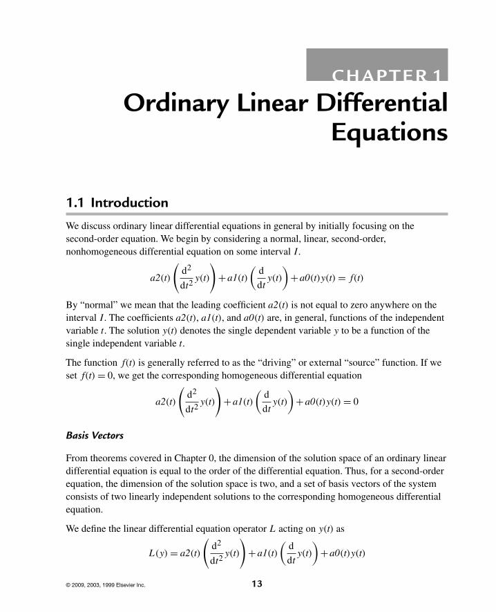
1.1 Introduction
We discuss ordinary linear differential equations in general by initially focusing on thesecond-order equation. We begin by considering a normal, linear, second-order,nonhomogeneous differential equation on some interval I.
a2(t)
(d2
dt2y(t)
)+a1(t)
(d
dty(t)
)+a0(t)y(t) = f(t)
By “normal” we mean that the leading coefficient a2(t) is not equal to zero anywhere on theinterval I. The coefficients a2(t), a1(t), and a0(t) are, in general, functions of the independentvariable t. The solution y(t) denotes the single dependent variable y to be a function of thesingle independent variable t.
The function f(t) is generally referred to as the “driving” or external “source” function. If weset f(t) = 0, we get the corresponding homogeneous differential equation
a2(t)
(d2
dt2y(t)
)+a1(t)
(d
dty(t)
)+a0(t)y(t) = 0
Basis Vectors
From theorems covered in Chapter 0, the dimension of the solution space of an ordinary lineardifferential equation is equal to the order of the differential equation. Thus, for a second-orderequation, the dimension of the solution space is two, and a set of basis vectors of the systemconsists of two linearly independent solutions to the corresponding homogeneous differentialequation.
We define the linear differential equation operator L acting on y(t) as
L(y) = a2(t)
(d2
dt2y(t)
)+a1(t)
(d
dty(t)
)+a0(t)y(t)
© 2009, 2003, 1999 Elsevier Inc. 13

14 Chapter 1
A basis of the system consists of two solution vectors y1(t) and y2(t), which are linearlyindependent and each of which satisfies the corresponding homogeneous equations L(y1) = 0and L(y2) = 0. There are an infinite number of legitimate sets of basis vectors of the system.However, all of the sets can be shown to be linearly dependent on each other.
The test for linear independence of the two vectors y1(t) and y2(t) on the interval I is thatthe Wronskian W(y1(t), y2(t)) does not equal zero at any point on the interval. Recall, theWronskian W(y1(t), y2(t)) is given as
W(y1(t), y2(t)) = y1(t)
(d
dty2(t)
)−y2(t)
(d
dty1(t)
)
If y1(t) and y2(t) are solutions of the homogeneous differential equation—that is, L(y1) = 0and L(y2) = 0—and their Wronskian W(y1(t), y2(t)) does not vanish at any point on theinterval, then these two vectors form a basis of the system on that interval.
If L is normal on the interval I and if y1(t) and y2(t) are the basis vectors of the system, then wesay these two vectors form a “complete” set. This is equivalent to saying that they completely“span” the solution space to the homogeneous differential equation. Thus, the general solutionto the homogeneous equation yh(t) is given as the linear superposition of the basis vectors
yh(t) = C1y1(t)+C2y2(t)
In the preceding, C1 and C2 are arbitrary constants.
If we denote a particular solution to the nonhomogeneous differential equation as yp(t), thenthe general solution to the nonhomogeneous equation can be written as a sum of the precedinghomogeneous solution plus the particular solution
y(t) = yh(t)+yp(t)
We will eventually show that a particular solution to the corresponding nonhomogeneousdifferential equation can be constructed from a set of basis vectors of the system.
1.2 First-Order Linear Differential Equations
We consider the first-order linear nonhomogeneous differential equation that is normal on aninterval I and that has the form
a1(t)
(d
dty(t)
)+a0(t) y(t) = f(t)
The corresponding first-order homogeneous equation can be written as
a1(t)
(d
dty(t)
)+a0(t) y(t) = 0

Ordinary Linear Differential Equations 15
The single basis vector solution to this homogeneous differential equation is
y1(t) = e∫ (
− a0(t)a1(t)
)dt
DEMONSTRATION: We seek the basis vector solution to the first-order linear homogeneousdifferential equation
t2(
d
dty(t)
)+3ty(t) = 0
SOLUTION: We identify the coefficients of the differential equation to be a1(t) = t2 anda0(t) = 3t. Note that the differential equation is not normal at the origin. The single systembasis vector is given by the integral
y1(t) = e∫ (
− 3t
)dt
This evaluates to be
y1(t) = 1
t3
for t �= 0. We can check this answer by substituting it back into the differential equation.
We now focus on the solution to the corresponding nonhomogeneous differential equation. Weassume the solution to the nonhomogeneous differential equation to be a nonlinear multiple ofthis basis vector, and we set
y(t) = u(t)y1(t)
Here, u(t) is some unknown, variable function of t [we are forcing a condition of linearindependence between y(t) and y1(t)]. Substituting this assumed solution into the differentialequation, we get
a1(t)
(d
dtu(t)
)y1(t)+a1(t)u(t)
(d
dty1(t)
)+a0(t)u(t)y1(t) = f(t)
Recognizing that y1(t) is a solution to the homogeneous differential equation—that is,L(y1) = 0—the last two preceding terms vanish, and we get a first-order equation in u(t) thatreads
d
dtu(t) = f(t)
a1(t) y1(t)
A simple integration of the preceding yields
u(t) =∫
f(t)
a1(t) y1(t)dt

16 Chapter 1
Thus, a particular solution to the nonhomogeneous differential equation can be written as theproduct of u(t) and y1(t) shown next:
yp(t) = y1(t)
(∫f(t)
a1(t) y1(t)dt
)
If we define the first-order Green’s function G1(t, s) as
G1(t, s) = y1(t)
a1(s) y1(s)
then we can express our particular solution in terms of the preceding Green’s function as
yp(t) =∫
G1(t, s)f(s) ds (1.1)
Writing the solution in terms of the Green’s function illustrates its general usefulness in thatonce the Green’s function for a particular differential equation is evaluated, the solution canaccommodate any type of driving or source function f(t).
DEMONSTRATION: We seek the solution to the first-order linear nonhomogeneousdifferential equation
t2(
d
dty(t)
)+3 ty(t) = f(t)
SOLUTION: From the preceding, we identify a1(t) = t2 and a0(t) = 3 t. The single basis
vector is
y1(t) = e∫ (
− a0(t)a1(t)
)dt
which evaluates to
y1(t) = 1
t3
From knowledge of the basis vector, we constuct the first-order Green’s function
G1(t, s) = y1(t)
a1(s)y1(s)
which evaluates to
G1(t, s) = s
t3

Ordinary Linear Differential Equations 17
The particular solution is the integral whose integrand is the product of the Green’s functionand the source function written in terms of the dummy variable s:
yp(t) =∫
sf(s)
t3ds
Thus, the general solution is
y(t) = C1
t3+
∫sf(s)
t3ds (1.2)
for t �= 0. Here, C1 is an arbitrary constant.
Care must be used in evaluating the preceding integral to ensure that we eventually get ananswer that is dependent only on t. The correct procedure is to first perform the integrationwith respect to the dummy variable s and then substitute t back in for s. This is illustrated in theworked-out examples that follow.
As the preceding solution stands, we can appreciate its generality in that it can accommodateany source function f(t). This is in dramatic contrast with the cumbersome method ofundetermined coefficients whereby one makes a trial-and-error guess at the solution.
We have completed the development of the solution to all first-order linear differentialequations. These solutions will be useful later in the development of solutions to partialdifferential equations. We now consider some example problems using Maple.
EXAMPLE 1.2.1: We seek a solution to the first-order linear nonhomogeneous differentialequation
d
dty(t)+y(t) = et
SOLUTION: We identify the coefficients and the driving function
> restart: a1(t):=1;a0(t):=1;
a1(t) := 1
a0(t) := 1 (1.3)
> f(t):=exp(t);f(s):=subs(t=s,f(t)):
f(t) := et (1.4)
System basis vector
> y1(t):=exp(int(−a0(t)/a1(t),t));
y1(t) := e−t (1.5)

18 Chapter 1
First-order Green’s function
> G1(t,s):=simplify(y1(t)/(subs(t=s,a1(t)*y1(t))));
G1 (t, s) := e−t+s (1.6)
Particular solution (integrate first with respect to s and then substitute s with t)
> y[p](t):=Int(G1(t,s)*f(s),s);
yp(t) :=∫
e−t+sesds (1.7)
> y[p](t):=subs(s=t, value(%));
yp(t) := 1
2et (1.8)
General solution: here, C1 is an arbitrary constant.
> y(t):=C1*y1(t)+y[p](t);
y(t) := C1e−t + 1
2et (1.9)
Check: Using Maple dsolve command.
> restart:ode:=diff(y(t),t)+y(t)=exp(t):dsolve(ode);
y(t) = 1
2et + e−t_C1 (1.10)
EXAMPLE 1.2.2: We seek the solution to the first-order linear differential equation
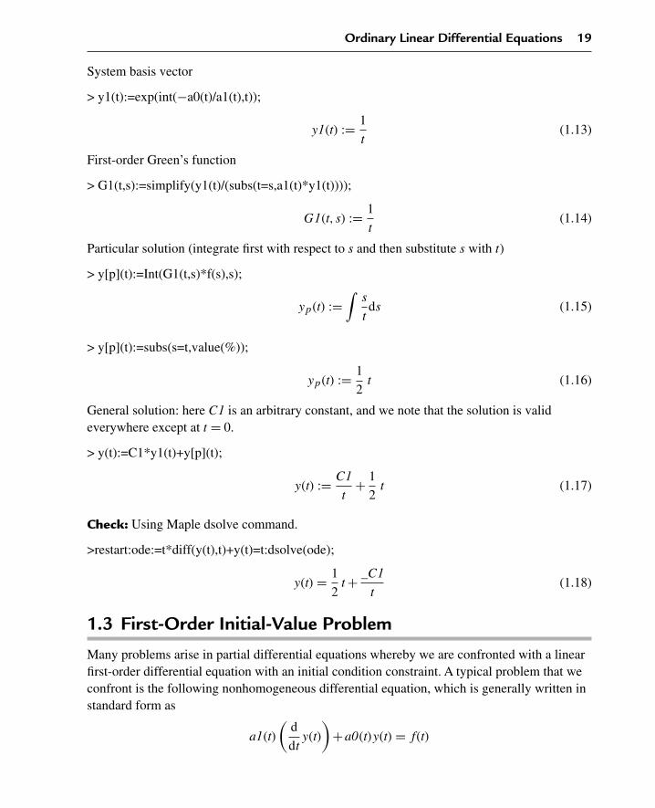
t
(d
dty(t)
)+y(t) = t
SOLUTION: We identify the coefficients and the driving function
> restart:a1(t):=t;a0(t):=1;
a1(t) := t
a0(t) := 1 (1.11)
> f(t):=t;f(s):=subs(t=s,f(t)):
f(t) := t (1.12)
Ordinary Linear Differential Equations 19
System basis vector
> y1(t):=exp(int(−a0(t)/a1(t),t));
y1(t) := 1
t(1.13)
First-order Green’s function
> G1(t,s):=simplify(y1(t)/(subs(t=s,a1(t)*y1(t))));
G1(t, s) := 1
t(1.14)
Particular solution (integrate first with respect to s and then substitute s with t)
> y[p](t):=Int(G1(t,s)*f(s),s);
yp(t) :=∫
s
tds (1.15)
> y[p](t):=subs(s=t,value(%));
yp(t) := 1
2t (1.16)
General solution: here C1 is an arbitrary constant, and we note that the solution is valideverywhere except at t = 0.
> y(t):=C1*y1(t)+y[p](t);
y(t) := C1
t+ 1
2t (1.17)
Check: Using Maple dsolve command.
>restart:ode:=t*diff(y(t),t)+y(t)=t:dsolve(ode);
y(t) = 1
2t + _C1
t(1.18)
1.3 First-Order Initial-Value Problem
Many problems arise in partial differential equations whereby we are confronted with a linearfirst-order differential equation with an initial condition constraint. A typical problem that weconfront is the following nonhomogeneous differential equation, which is generally written instandard form as
a1(t)
(d
dty(t)
)+a0(t)y(t) = f(t)

20 Chapter 1
We seek a solution that satisfies the initial (time t = 0) condition y(0) = y0. We now write ourbasis vector in terms of the following definite integral
y1(t) = e∫ t
0
(− a0(s)
a1(s)
)ds
In Section 1.2, the first-order Green’s function was shown to be
G1(t, s) = y1(t)
a1(s)y1(s)
In terms of the Green’s function, the particular solution is
yp(t) =t∫
0
G1(t, s)f(s)ds
and our final general solution to the initial value problem becomes
y(t) = C1y1(t)+t∫
0
G1 (t, s) f(s)ds
From the initial condition constraint y(0) = y0, the arbitrary constant C1 is evaluated to be
C1 = y0
Thus, the final solution, which satisfies the initial condition constraint, is given as
y(t) = y0e∫ t
0
(− a0(s)
a1(s)
)ds +
t∫0
G1(t, s)f(s)ds (1.19)
Because we forced the initial condition, there is no arbitrary constant in the solution, and wesee that the preceding form of the solution can accommodate any initial condition and anydriving function f(t).
EXAMPLE 1.3.1: We consider an object whose rate of thermal cooling obeys Newton’s lawwhereby the rate of change of the temperature of the body is proportional to the differencebetween the temperature of the body and the temperature of its surroundings. Consider aspecific problem whereby the initial temperature of the body is 100°C, the surroundingtemperature is 20°C, and the thermal coefficient of diffusivity is k = 0.2/ sec. We seek y(t): thetemperature of the object as a function of the time t.
SOLUTION: The defining differential equation of the system (see Exercise 1.13 at the end ofthe chapter) is
d
dty(t) = −k(y(t)−20)

Ordinary Linear Differential Equations 21
Inserting the value for k, we rewrite the preceding in the standard form
d
dty(t)+ 2y(t)
10= 4
We can identify the coefficients of the differential equation as
> restart:a1(t):=1;a0(t):=2/10;
a1(t) := 1
a0(t) := 1
5(1.20)
Initial condition
> y(0):=100;
y(0) := 100 (1.21)
The driving function is
> f(t):=4;f(s):=subs(t=s,f(t)):
f(t) := 4 (1.22)
System basis vector
> y1(t):=exp(int(subs(t=s,−a0(t)/a1(t)),s=0..t));
y1(t) := e− 15 t (1.23)
First-order Green’s function
> G1(t,s):=simplify(y1(t)/(subs(t=s,a1(t)*y1(t))));
G1(t, s) := e− 15 t + 1
5 s (1.24)
Particular solution
> y[p](t):=Int(G1(t,s)*f(s),s=0..t);
yp(t) :=t∫
0
4 e− 15 t + 1
5 s ds (1.25)
> y[p](t):=value(%);
yp(t) := −20 e− 15 t +20 (1.26)

22 Chapter 1
Final solution
> y(t):=simplify(eval(y(0)*y1(t)+y[p](t)));
y(t) := 80 e− 15 t +20 (1.27)
> plot(y(t),t=0..20,thickness=10);
t0 5 10 15 20
30405060708090
100
Figure 1.1
Figure 1.1 depicts the decay of the temperature of the body until it approaches the surroundingtemperature. We can provide an animated view of the temperature decay as follows:
ANIMATION
> y(x,t):=y(t)*(Heaviside(x+1/2)−Heaviside(x−1/2));
y(x, t) :=(
80 e− 15 t +20
) (Heaviside
(x+ 1
2
)−Heaviside
(x− 1
2
))(1.28)
> with(plots):animate(y(x,t),x=−1..1,t=0..30,thickness=2);
From Figure 1.1, we can see the actual real-time decay of the temperature until it finallyreaches its surrounding temperature.
Check: Using Maple dsolve command with initial conditions.
> restart:ode:=diff(y(t),t)+2/10*y(t)=4;
ode := d
dty(t)+ 1
5y(t) = 4 (1.29)
> ics:=y(0)=100;
ics := y(0) = 100 (1.30)
> dsolve({ode,ics});
y(t) = 20+80 e− 15 t (1.31)

Ordinary Linear Differential Equations 23
1.4 Second-Order Linear Differential Equations withConstant Coefficients
We now consider second-order linear nonhomogeneous differential equations with constantcoefficients on some interval I. The equation, written in standard form, reads
a2
(d2
dt2y(t)
)+a1
(d
dty(t)
)+a0 y(t) = f(t)
Since the order of the differential equation is two, we must first find a set of two basis vectorsof the corresponding homogeneous differential equation
a2
(d2
dt2y(t)
)+a1
(d
dty(t)
)+a0 y(t) = 0
Since the coefficients a2, a1, and a0 are time invariant (constants), the method of undeterminedcoefficients can be used to find a set of system basis vectors. We assume a solution of the form
y(t) = ert
Substitution of this into the homogeneous equation provides us with the “characteristic”equation
a2 r2 +a1 r +a0 = 0
The roots of the characteristic equation are given as
r1 = −a1+√
a12 −4a2a0
2a2
r2 = −a1−√
a12 −4a2a0
2a2
Thus, our two solution vectors become
y1(t) = e
(−a1+
√a12 − 4a2a0
)t
2a2
and
y2(t) = e
(−a1−
√a12 − 4a2a0
)t
2a2 (1.32)
It can be shown that if the discriminant given here is not equal to 0, then the roots r1 and r2are distinct and the two solutions are linearly independent; thus, for constant coefficientsecond-order differential equations, the preceding solution vectors constitute a set of systembasis vectors.

24 Chapter 1
DEMONSTRATION: We seek a set of basis vectors for the second-order linear homogeneousdifferential equation with constant coefficients as shown:
d2
dt2y(t)+3
(d
dty(t)
)+2y(t) = 0
SOLUTION: We identify the coefficients of the differential equation a2 = 1, a1 = 3, and
a0 = 2. The characteristic equation is
(r +2)(r +1) = 0
The roots of the characteristic equation are given as r1 = −2 and r2 = −1. Thus, a set ofsystem basis vectors is
y1(t) = e−2 t
and
y2(t) = e−t
We now consider a very special case of a differential equation with constant coefficients.
The Euler Differential Equation
One of the most frequently occurring ordinary differential equations, which arises in thesolution of partial differential equations in the rectangular coordinate system, is the Eulerdifferential equation. This differential equation is a special case of a second-order linearequation with constant coefficients. The general homogeneous form of this equation reads
d2
dt2y(t)+λy(t) = 0
Note that the equation lacks a first-order derivative term. We now consider some exampleproblems of the Euler differential equation.
EXAMPLE 1.4.1: Find a set of basis vectors for the Euler differential equation with a positivecoefficient.
d2
dt2y(t)+μ2y(t) = 0
SOLUTION: We identify the coefficients
> restart:a2:=1;a1:=0;a0:=muˆ2;
a2 := 1
a1 := 0 (1.33)
a0 := μ2

Ordinary Linear Differential Equations 25
Characteristic equation
> eq:=factor(a2*rˆ2+a1*r+a0=0);
eq := r2 +μ2 = 0 (1.34)
The roots of the characteristic equation are given as
> con:=solve(eq,r):r1:=con[1];r2:=con[2];
r1 := Iμ(1.35)
r2 := −Iμ
System basis vectors
> y1(t):=evalc(Im(exp(r1*t)));
y1(t) := sin(μt) (1.36)
> y2(t):=evalc(Re(exp(r2*t)));
y2(t) := cos(μt) (1.37)
General solution: here C1 and C2 are arbitrary constants.
> y(t):=C1*y1(t)+C2*y2(t);
y(t) := C1 sin(μt)+C2 cos(μt) (1.38)
Check: Using Maple dsolve command.
> restart:ode:=diff(y(t),t,t)+muˆ2*y(t)=0:dsolve(ode);
y(t) = _C1 sin (μt)+_C2 cos(μt) (1.39)
EXAMPLE 1.4.2: Find a set of basis vectors for the Euler differential equation with negativecoefficient.
d2
dt2y(t)−μ2y(t) = 0
SOLUTION: We identify the coefficients
> restart:a2:=1;a1:=0;a0:=−muˆ2;
a2 := 1
a1 := 0
a0 := −μ2 (1.40)

26 Chapter 1
Characteristic equation
> eq:=factor(a2*rˆ2+a1*r+a0=0);
eq := −(μ− r)(μ+ r) = 0 (1.41)
The roots of the characteristic equation are given as
> con:=solve(eq,r):r1:=con[1];r2:=con[2];
r1 := μ
r2 := −μ (1.42)
System basis vectors
> y1(t):=exp(r1*t);
y1(t) := eμt (1.43)
> y2(t):=exp(r2*t);
y2(t) := e−μt (1.44)
General solution: here C1 and C2 are arbitrary constants.
> y(t):=C1*y1(t)+C2*y2(t);
y(t) := C1eμt +C2e−μt (1.45)
Check: Using Maple dsolve command.
> restart:ode:=diff(y(t),t,t)−muˆ2*y(t)=0:dsolve(ode);
y(t) = _C1 eμt +_C2 e−μt (1.46)
In application problems in partial differential equations, it is more convenient to express thisset of basis vectors in the (linearly dependent) equivalent form:
> y1(t):=sinh(mu*t);
y1(t) := sinh(μt) (1.47)
> y1(t):=cosh(mu*t);
y2(t) := cosh(μt) (1.48)
We now consider the following example, which occurs in the solution of the time-dependentportion of the wave partial differential equation that we will look at later.

Ordinary Linear Differential Equations 27
EXAMPLE 1.4.3: Find the basis vectors for the equation
d2
dt2y(t)+γ
(d
dty(t)
)+ c2λy(t) = 0
SOLUTION: We identify the coefficients
> restart:a2:=1;a1:=gamma;a0:=cˆ2*lambda;
a2 := 1
a1 := γ
a0 := c2λ (1.49)
Characteristic equation
> eq:=factor(a2*rˆ2+a1*r+a0=0);
eq := r2 +γ r + c2λ = 0 (1.50)
The roots of the characteristic equation are given as
> con:=solve(eq,r):r1:=con[1];r2:=con[2];
r1 := − 1
2γ + 1
2
√γ2 −4 c2λ
r2 := − 1
2γ − 1
2
√γ2 −4 c2λ (1.51)
System basis vectors
> y1(t):=exp(r1*t);
y1(t) := e
(− 1
2 γ+ 12
√γ2−4c2λ
)t
(1.52)
> y2(t):=exp(r2*t);
y2(t) := e
(− 1
2 γ− 12
√γ2−4c2λ
)t
(1.53)
General solution: here C1 and C2 are arbitrary constants.
> y(t):=C1*y1(t)+C2*y2(t);
y(t) := C1e
(− 1
2 γ+ 12
√γ2−4c2λ
)t +C2e
(− 1
2 γ− 12
√γ2−4c2λ
)t
(1.54)

28 Chapter 1
Check: Using Maple dsolve command.
> restart:ode:=diff(y(t),t,t)+gamma*diff(y(t),t)+cˆ2*lambda*y(t)=0:dsolve(ode);
y(t) = _C1 e
(− 1
2 γ+ 12
√γ2−4 c2λ
)t +_C2 e
(− 1
2 γ− 12
√γ2−4 c2λ
)t
(1.55)
For the case where γ is very small, the discriminant given is negative, and we end up withcomplex roots. For this situation, it is more convenient to express this set of basis vectors in the(linearly dependent) equivalent form:
> y1(t):=exp(−gamma/2*t)*cos(sqrt(lambda*cˆ2−gammaˆ2/4)*t);
y1(t) := e− 12 γt cos
(1
2
√−γ2 +4c2λt
)(1.56)
> y2(t):=exp(−gamma/2*t)*sin(sqrt(lambda*cˆ2−gammaˆ2/4)*t);
y2(t) := e− 12 γt sin
(1
2
√−γ2 +4c2λt
)(1.57)
In the preceding paragraphs, we considered the special case of differential equations withconstant coefficients. In general, the coefficients of linear differential equations are notconstants and are functionally dependent on the independent variable. We now look at thegeneral case of variable coefficients.
1.5 Second-Order Linear Differential Equations withVariable Coefficients
We now consider second-order linear nonhomogeneous differential equations with variablecoefficients on a finite interval I. The equation written in standard form reads as
a2(t)
(d2
dt2y(t)
)+a1(t)
(d
dty(t)
)+a0(t)y(t) = f(t)
We note that the generalized coefficients a2(t), a1(t), and a0(t) are not constant. They arefunctionally dependent on the independent variable t; thus, the method of undeterminedcoefficients cannot be used here to find the basis vectors.
Since the order of the differential equation is two, we must first find two basis vectors of thecorresponding homogeneous differential equation.
a2(t)
(d2
dt2y(t)
)+a1(t)
(d
dty(t)
)+a0(t)y(t) = 0
Different types of variable coefficient differential equations demand their own peculiartechnique for solution. We now consider a prominent example of such an equation.

Ordinary Linear Differential Equations 29
The Cauchy-Euler Differential Equation
We consider the special case of the Cauchy-Euler differential equation, which will occur laterin our study of partial differential equations in the cylindrical coordinate system.
The nonhomogeneous Cauchy-Euler differential equation has the form
a2 t2
(d2
dt2y(t)
)+a1t
(d
dty(t)
)+a0 y(t) = f(t)
where a2, a1, and a0 are constants, and the t-dependence of each term has been extractedexplicitly. This differential equation is easily recognized by the fact that the power of thecoefficient of the independent variable t in each term is equal to the order of differentiation ofthe term y(t), which it multiplies.
We now consider finding a set of basis vectors for the corresponding homogeneousCauchy-Euler equation
a2 t2
(d2
dt2y(t)
)+a1 t
(d
dty(t)
)+a0 y(t) = 0
We substitute an assumed solution of the form
y(t) = tm
into the homogeneous differential equation and get the characteristic equation
a2m(m−1)+a1m+a0 = 0
Solving for the roots of this equation, we get
m1 = a2−a1+√
a22 −2a2a1+a12 −4a2a0
2a2
and
m2 = a2−a1−√
a22 −2a2a1+a12 −4a2a0
2a2
Thus, the solution vectors to the Cauchy-Euler dfferential equation are
y1(t) = ta2−a1+
√a22−2a2a1+a12−4a2a0
2a2
and
y2(t) = ta2−a1−
√a22−2a2a1+a12−4a2a0
2a2
30 Chapter 1
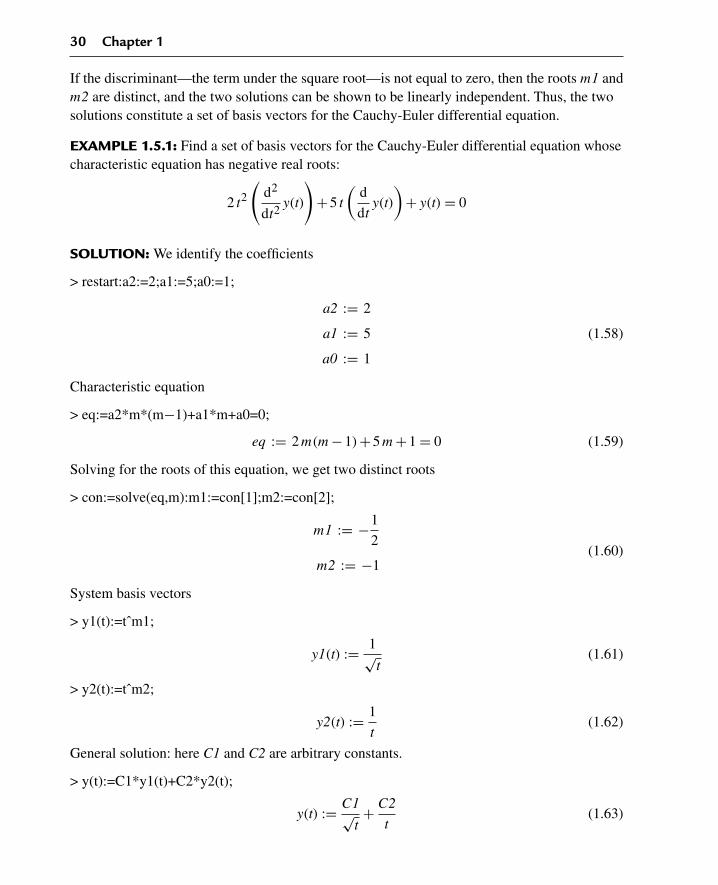
If the discriminant—the term under the square root—is not equal to zero, then the roots m1 andm2 are distinct, and the two solutions can be shown to be linearly independent. Thus, the twosolutions constitute a set of basis vectors for the Cauchy-Euler differential equation.
EXAMPLE 1.5.1: Find a set of basis vectors for the Cauchy-Euler differential equation whosecharacteristic equation has negative real roots:
2 t2
(d2
dt2y(t)
)+5 t
(d
dty(t)
)+y(t) = 0
SOLUTION: We identify the coefficients
> restart:a2:=2;a1:=5;a0:=1;
a2 := 2
a1 := 5 (1.58)
a0 := 1
Characteristic equation
> eq:=a2*m*(m−1)+a1*m+a0=0;
eq := 2m(m−1)+5m+1 = 0 (1.59)
Solving for the roots of this equation, we get two distinct roots
> con:=solve(eq,m):m1:=con[1];m2:=con[2];
m1 := −1
2(1.60)
m2 := −1
System basis vectors
> y1(t):=tˆm1;
y1(t) := 1√t
(1.61)
> y2(t):=tˆm2;
y2(t) := 1
t(1.62)
General solution: here C1 and C2 are arbitrary constants.
> y(t):=C1*y1(t)+C2*y2(t);
y(t) := C1√t+ C2
t(1.63)

Ordinary Linear Differential Equations 31
Check: Using Maple dsolve command.
> restart:ode:=2*tˆ2*diff(y(t),t,t)+5*t*diff(y(t),t)+y(t)=0:dsolve(ode);
y(t) = _C1√t
+ _C2√t
(1.64)
EXAMPLE 1.5.2: Find the basis vectors for the following Cauchy-Euler differential equationwhose characteristic equation has complex roots:
t2
(d2
dt2y(t)
)+ t
(d
dty(t)
)+4y(t) = 0
SOLUTION: We identify the coefficients
> restart:a2:=1;a1:=1;a0:=4;
a2 := 1
a1 := 1 (1.65)
a0 := 4
Characteristic equation
> eq:=a2*m*(m−1)+a1*m+a0=0;
eq := m(m−1)+m+4 = 0 (1.66)
Solving for the roots of this equation, we get two distinct roots
> con:=solve(eq,m):m1:=con[1];m2:=con[2];
m1 := 2I (1.67)
m2 := −2I
System basis vectors
> y1(t):=tˆm1;
y1(t) := t2I (1.68)
> y2(t):=tˆm2;
y2(t) := t−2I (1.69)
General solution: here C1 and C2 are arbitrary constants.
> y(t):=C1*y1(t)+C2*y2(t);
y(t) := C1t2I +C2t−2I (1.70)

32 Chapter 1
For convenience later on, we express the preceding set of basis vectors in the (linearlydependent) equivalent form:
> y1(t):=sin(2*ln(t));
y1(t) := sin(2 ln(t)) (1.71)
> y2(t):=cos(2*ln(t));
y2(t) := cos(2 ln(t)) (1.72)
General solution: here C1 and C2 are arbitrary constants.
> y(t):=C1*y1(t)+C2*y2(t);
y(t) := C1 sin(2 ln(t))+C2 cos(2 ln(t)) (1.73)
Check: Using Maple dsolve command.
> restart:ode:=tˆ2*diff(y(t),t,t)+t*diff(y(t),t)+4*y(t)=0:dsolve(ode);
y(t) = _C1 sin(2 ln(t))+_C2 cos(2 ln(t)) (1.74)
1.6 Finding a Second Basis Vector by the Method ofReduction of Order
In some cases, a second linearly independent solution vector does not always become readilyavailable. Generally, this occurs if any of the preceding discriminants vanish; in this case, wedo not get two distinct roots. However, if we know one solution vector for the second-orderlinear differential equation, then the method of reduction of order can be used to find a secondlinearly independent solution vector.
Let y1(t) be one solution to the homogeneous differential equation:
a2(t)
(d2
dt2y1(t)
)+a1(t)
(d
dty1(t)
)+a0(t)y1(t) = 0
Using operator notation, we write the preceding equation as L(y1) = 0. We now assume that asecond solution y2(t) can be expressed as a nonlinear multiple of y1(t):
y2(t) = u(t)y1(t)

Ordinary Linear Differential Equations 33
Substituting this into the preceding homogeneous differential equation yields
a2(t)
(d2
dt2u(t)
)y1(t)+2a2(t)
(d
dtu(t)
)(d
dty1(t)
)+a2(t)u(t)
(d2
dt2y1(t)
)
+a1(t)
(d
dtu(t)
)y1(t)+a1(t)u(t)
(d
dty1(t)
)+a0(t)u(t)y1(t) = 0
Collecting terms, we get(a2(t)
(d2
dt2y1(t)
)+a1(t)
(d
dty1(t)
)+a0(t)y1(t)
)u(t)+a2(t)
(d2
dt2u(t)
)y1(t)
+2a2(t)
(d
dtu(t)
)(d
dty1(t)
)+a1(t)
(d
dtu(t)
)y1(t) = 0
Since y1(t) satisfies the homogeneous equation—that is, L(y1) = 0—then the first term abovevanishes, and we end up with the following homogeneous differential equation
a2(t)
(d2
dt2u(t)
)y1(t)+
(a1(t)y1(t)+2a2(t)
(d
dty1(t)
))(d
dtu(t)
)= 0
This is basically a first-order linear differential equation in terms of the first derivative of u(t).We have reduced the order of the differential equation. From the solution procedure for allfirst-order linear equations in Section 1.2, we solve for u(t) and get
u(t) =∫
e
∫ (− a1(t)
a2(t)− 2
(ddt
y1(t))
y1(t)
)dt
dt
Simplifying the preceding yields
u(t) =∫
e−
(∫a1(t)a2(t)
dt)
y1(t)2dt
Thus, our second solution y2(t) is given as
y2(t) = y1(t)
⎛⎜⎝∫
e−
(∫a1(t)a2(t)
dt)
y1(t)2dt
⎞⎟⎠
This solution can be shown to be linearly independent of y1(t). Thus, from one solution y1(t),the method of reduction of order allows us to generate a second basis vector y2(t).
DEMONSTRATION: Use the method of reduction of order to determine a set of basis vectorsfor the Cauchy-Euler differential equation
t2
(d2
dt2y(t)
)−3t
(d
dty(t)
)+3y(t) = 0
34 Chapter 1
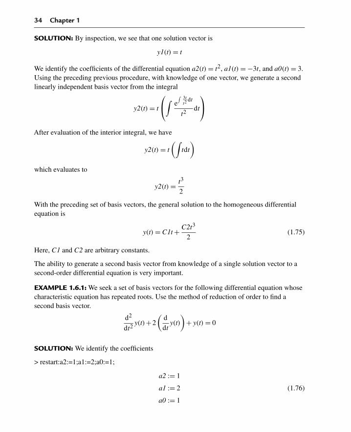
SOLUTION: By inspection, we see that one solution vector is
y1(t) = t
We identify the coefficients of the differential equation a2(t) = t2, a1(t) = −3t, and a0(t) = 3.Using the preceding previous procedure, with knowledge of one vector, we generate a secondlinearly independent basis vector from the integral
y2(t) = t
⎛⎝∫
e∫ 3t
t2dt
t2dt
⎞⎠
After evaluation of the interior integral, we have
y2(t) = t
(∫tdt
)
which evaluates to
y2(t) = t3
2
With the preceding set of basis vectors, the general solution to the homogeneous differentialequation is
y(t) = C1t + C2t3
2(1.75)
Here, C1 and C2 are arbitrary constants.
The ability to generate a second basis vector from knowledge of a single solution vector to asecond-order differential equation is very important.
EXAMPLE 1.6.1: We seek a set of basis vectors for the following differential equation whosecharacteristic equation has repeated roots. Use the method of reduction of order to find asecond basis vector.
d2
dt2y(t)+2
(d
dty(t)
)+y(t) = 0
SOLUTION: We identify the coefficients
> restart:a2:=1;a1:=2;a0:=1;
a2 := 1
a1 := 2 (1.76)
a0 := 1

Ordinary Linear Differential Equations 35
We assume a solution
> y(t):=exp(r*t);
y(t) := ert (1.77)
Characteristic equation
> eq:=factor(a2*diff(y(t),t,t)+a1*diff(y(t),t)+a0*y(t))/exp(r*t)=0;
eq := (r +1)2 = 0 (1.78)
The roots of the characteristic equation are given as
> con:=solve(eq,r):r1:=con[1];r2:=con[2];
r1 := −1 (1.79)
r2 := −1
This is a situation whereby the discriminant is 0, and we get two equal roots from thecharacteristic equation. The situation of two equal roots does not provide us with theopportunity to get two linearly independent solutions. To get a second linearly independentsolution vector, we declare one basis vector to be
> y1(t):=exp(r1*t);
y1(t) := e−t (1.80)
Using the preceding method of reduction of order, we obtain a second basis vector
> y2(t):=y1(t)*int(exp(−int(a1/a2,t))/y1(t)ˆ2,t);
y2(t) := e−t t (1.81)
General solution: here C1 and C2 are arbitrary constants.
> y(t):=C1*y1(t)+C2*y2(t);
y(t) := C1e−t +C2e−t t (1.82)
Check: Using Maple dsolve command.
> restart:ode:=diff(y(t),t,t)+2*diff(y(t),t)+y(t)=0:dsolve(ode);
y(t) = _C1e−t +_C2e−t t (1.83)
EXAMPLE 1.6.2: We seek the solution to the following second-order linear differentialequation with trigonometric coefficients:
d2
dt2y(t)+ (tan(t)−2 cot(t))
(d
dty(t)
)= 0

36 Chapter 1
SOLUTION: We identify the coefficients
> restart:a2(t):=1;a1(t):=tan(t)−2*cot(t);a0(t):=0;
a2(t) := 1
a1(t) := tan(t)−2 cot(t) (1.84)
a0(t) := 0
By inspection, we see that one solution is
> y1(t):=1;
y1(t) := 1 (1.85)
Using the method of reduction of order, we generate a second basis vector
> y2(t):=y1(t)*int(exp(−int(a1(t)/a2(t),t))/y1(t)ˆ2,t);
y2(t) := 1
3sin(t)3 (1.86)
General solution: here C1 and C2 are arbitrary constants.
> y(t):=C1*y1(t)+C2*y2(t);
y(t) := C1+ 1
3C2 sin(t)3 (1.87)
Check: Using Maple dsolve command.
> restart:ode:=diff(y(t),t,t)+(tan(t)−2*cot(t))*diff(y(t),t)=0:dsolve(ode);
y(t) = _C1+ sin(t)3_C2 (1.88)
1.7 The Method of Variation of Parameters—Second-OrderGreen’s Function
We now consider finding a particular solution to a second-order linear nonhomogeneousdifferential equation on an interval I. By the method of variation of parameters, we willconstruct this solution from a known set of basis vectors of the system. Recall that the basisvectors of the second-order system are two linearly independent solutions of the correspondinghomogeneous system.
The second-order linear nonhomogeneous differential equation reads as
a2(t)
(d2
dt2y(t)
)+a1(t)
(d
dty(t)
)+a0(t)y(t) = f(t)

Ordinary Linear Differential Equations 37
Similar to what we did for the first-order system, we assume our particular solution to thesecond-order nonhomogeneous equation to be a nonlinear superposition of the two basisvectors y1(t) and y2(t)—that is, we set
y(t) = u1(t)y1(t)+u2(t)y2(t) (1.89)
Here, u1(t) and u2(t) are two unknown functions of the independent variable t for which wenow seek their solutions. Taking the first derivative of the preceding using the product ruleyields
d
dty(t) = u1(t)
(d
dty1(t)
)+y1(t)
(d
dtu1(t)
)+u2(t)
(d
dty2(t)
)+y2(t)
(d
dtu2(t)
)
To simplify our solution, we set
y1(t)
(d
dtu1(t)
)+y2(t)
(d
dtu2(t)
)= 0
Taking the second derivative of the remaining term and substituting into the precedingnonhomogeneous differential equation and collecting terms yields(
a2(t)
(d2
dt2y1(t)
)+a1(t)
(d
dty1(t)
)+a0(t)y1(t)
)u1(t)+
(a2(t)
(d2
dt2y2(t)
)
+ a1(t)
(d
dty2(t)
)+a0(t)y2(t)
)u2(t)+a2(t)
((d
dtu1(t)
)y1(t)+
(d
dtu2(t)
)y2(t)
)= f(t)
Since y1(t) and y2(t) are both solutions to the homogeneous equation—that is, L(y1) = 0 andL(y2) = 0—the first two preceding terms vanish, and we arrive at
a2(t)
((d
dtu1(t)
)y1(t)+
(d
dtu2(t)
)y2(t)
)= f(t)
Thus, we finally end up with a system of two differential equations(d
dtu1(t)
)y1(t)+
(d
dtu2(t)
)y2(t) = 0
and (d
dtu1(t)
)(d
dty1(t)
)+
(d
dtu2(t)
)(d
dty2(t)
)= f(t)
a2(t)
Solving these two equations simultaneously, for the derivatives of u1(t) and u2(t), we arrive atthe two first-order linear nonhomogeneous differential equations:
d
dtu1(t) = − f(t)y2(t)
a2(t)
(y1(t)
(d
dty2(t)
)−y2(t)
(d
dty1(t)
))

38 Chapter 1
and
d
dtu2(t) = − f(t)y1(t)
a2(t)
(y1(t)
(d
dty2(t)
)−y2(t)
(d
dty1(t)
))
Integrating each of the preceding yields
u1(t) =∫ ⎛
⎜⎜⎝− f(t)y2(t)(−y2(t)
(d
dty1(t)
)+
(d
dty2(t)
)y1(t)
)a2(t)
⎞⎟⎟⎠dt
and
u2(t) =∫
− f(t)y1(t)(−y2(t)
(d
dty1(t)
)+
(d
dty2(t)
)y1(t)
)a2(t)
dt
Recognizing the denominator in the integrands as the Wronskian
W(y1(t), y2(t)) = −y2(t)
(d
dty1(t)
)+
(d
dty2(t)
)y1(t)
we get the following solutions
u1(t) = −(∫
f(t)y2(t)
a2(t)W(y1(t), y2(t))dt
)
and
u2(t) =∫
f(t)y1(t)
a2(t)W(y1(t), y2(t))dt
Thus, our particular solution to the differential equation becomes
yp(t) = y2(t)
(∫f(t)y1(t)
a2(t)W(y1(t), y2(t))dt
)−y1(t)
(∫f(t)y2(t)
a2(t)W(y1(t), y2(t))dt
)
Using the dummy variable s in the integrands, a more compact form of the particular solutioncan be rewritten as
yp(t) =∫
(y1(s)y2(t)−y1(t)y2(s))f(s)
a2(s)W(y1(s), y2(s))ds
Similar to what we did for first-order differential equations, we now define G2(t, s) as thesecond-order Green’s function
G2(t, s) = y1(s)y2(t)−y1(t)y2(s)
a2(s)W(y1(s), y2(s))(1.90)
Ordinary Linear Differential Equations 39
Of course, this result is valid only on an interval I, where the term a2(t) does not vanish—thatis, on an interval where the equation is normal. Further, since the vectors form a basis, they arelinearly independent, and the Wronskian is nonzero on this interval.
In terms of the second-order Green’s function given earlier, the particular solution takes onthe form
yp(t) =∫
G2(t, s)f(s)ds (1.91)
Again, we see that this form of the solution can accommodate any type of driving or sourcefunction f(t). This procedure, by way of the method of variation of parameters, leads to anintegral solution whereby the Green’s function acts as the kernel of the integrand.
The beauty of the preceding form just derived becomes apparent when we compare it with thealternate procedure of undetermined coefficients. In that procedure, we have to make atentative guess at the solution. The guess, of course, depends on the character of the sourcefunction f(t) and whether or not this function is linearly dependent on the system basis vectors.With the preceding method, there is no need to guess, and we get immediate solutions.
DEMONSTRATION: We seek the particular solution to the second-order linearnonhomogeneous differential equation
d2
dt2y(t)+2
(d
dty(t)
)+y(t) = te−t
SOLUTION: We identify the coefficients of the differential equation a2(t) = 1, a1(t) = 2, anda0(t) = 1, and the source term
f(t) = te−t
Earlier, from Example 1.6.1, we found a set of basis vectors to be
y1(t) = e−t
and
y2(t) = te−t
We note the linear dependence of the source term on one of the basis vectors. Evaluation of theWronskian of the basis yields
W(et , tet) = e−2t
Evaluation of the second-order Green’s function from the formula
G2(t, s) = y1(s)y2(t)−y1(t)y2(s)
a2(s)W(y1(s), y2(s))

40 Chapter 1
yields
G2(t, s) = e−ste−t − e−tse−s
e−2s
The particular solution is the integral whose integrand is the product of the Green’s functionand the source function written in terms of the dummy variable s:
yp(t) =∫
(e−ste−t − e−tse−s)se−s
e−2 sds (1.92)
Integrating first with respect to the dummy variable s and then substituting t for s yields
yp(t) = t3e−t
6
Thus, the general solution to the problem is the sum of the homogeneous plus the particularsolution. Here C1 and C2 are arbitary constants.
y(t) = C1e−t +C2 te−t + t3e−t
6(1.93)
The example just described is especially interesting because the source term f(t) is linearlydependent on one of the basis vectors. The ease with which we found this solution indicates themethod of variation of paramaters to be far more convenient than what we would haveencountered with the method of undetermined coefficients.
EXAMPLE 1.7.1: Use the method of variation of parameters to generate the particular solutionto the differential equation that is not normal at the origin.
t
(d2
dt2y(t)
)+ d
dty(t) = t +1
SOLUTION: We identify the coefficients
> restart:a2(t):=t;a1(t):=1;a0(t):=0;
a2(t) := t
a1(t) := 1
a0(t) := 0 (1.94)
Source term
> f(t):=t+1;
f(t) := t +1 (1.95)
From earlier methods, we see that one basis vector is a constant and a second basis vector canbe found using methods of Section 1.6. Thus, two possible basis vectors are
Ordinary Linear Differential Equations 41
> y1(t):=1;
y1(t) := 1 (1.96)
> y2(t):=ln(t);
y2(t) := ln(t) (1.97)
Wronskian
> W(y1(t),y2(t)):=y1(t)*diff(y2(t),t)−y2(t)*diff(y1(t),t);
W(1, ln(t)) := 1
t(1.98)
> y1(s):=subs(t=s,y1(t)):y2(s):=subs(t=s,y2(t)):W(y1(s),y2(s)):=subs(t=s,W(y1(t),y2(t))):a2(s):=subs(t=s,a2(t)):f(s):=subs(t=s,f(t)):
Green’s function
> G2(t,s):=(y1(s)*y2(t)−y1(t)*y2(s))/(a2(s)*W(y1(s),y2(s)));
G2(t, s) := ln(t)− ln(s) (1.99)
Particular solution (integrate first with respect to s and then substitute s with t)
> y[p](t):=Int(G2(t,s)*f(s),s);
yp(t) :=∫
(ln(t)− ln(s))(s+1)ds (1.100)
> y[p](t):=subs(s=t,value(%));
yp(t) := 1
4t2 + t (1.101)
General solution: here C1 and C2 are arbitrary constants.
> y(t):=C1*y1(t)+C2*y2(t)+y[p](t);
y(t) := C1+C2 ln(t)+ 1
4t2 + t (1.102)
This solution is valid everywhere except at the point t = 0. This follows, since the differentialequation fails to be normal at the origin.
Check: Using Maple dsolve command.
> restart:ode:=t*diff(y(t),t,t)+diff(y(t),t)=t+1:dsolve(ode);
y(t) = 1
4t2 +_C1 ln(t)+ t +_C2 (1.103)

42 Chapter 1
EXAMPLE 1.7.2: We seek the solution to the nonhomogeneous Euler differential equation
d2
dt2y(t)+y(t) = sec(t)
SOLUTION: We identify the coefficients
> restart:a2(t):=1;a1(t):=0;a0(t):=1;
a2(t) := 1
a1(t) := 0 (1.104)
a0(t) := 1
Source function
> f(t):=sec(t);
f(t) := sec(t) (1.105)
System basis vectors from earlier result
> y1(t):=sin(t);
y1(t) := sin(t) (1.106)
> y2(t):=cos(t);
y2(t) := cos(t) (1.107)
Wronskian
> W(y1(t),y2(t)):=simplify(y1(t)*diff(y2(t),t)−y2(t)*diff(y1(t),t));
W(sin(t), cos(t)) := −1 (1.108)
> y1(s):=subs(t=s,y1(t)):y2(s):=subs(t=s,y2(t)):W(y1(s),y2(s)):=subs(t=s,W(y1(t),y2(t))):a2(s):=subs(t=s,a2(t)):f(s):=subs(t=s,f(t)):
Green’s function
> G2(t,s):=(y1(s)*y2(t)−y1(t)*y2(s))/(a2(s)*W(y1(s),y2(s)));
G2(t, s) := − sin(s) cos(t)+ sin(t) cos(s) (1.109)
Particular solution (integrate first with respect to s and then substitute s with t)
> y[p](t):=Int(G2(t,s)*f(s),s);
yp(t) :=∫
(−sin(s) cos(t)+ sin(t) cos(s)) sec(s)ds (1.110)

Ordinary Linear Differential Equations 43
> y[p](t):=subs(s=t,value(%));
yp(t) := cos(t) ln(cos(t))+ sin(t)t (1.111)
General solution: here C1 and C2 are arbitrary constants.
> y(t):=C1*y1(t)+C2*y2(t)+y[p](t);
y(t) := C1 sin(t)+C2 cos(t)+ cos(t) ln(cos(t))+ sin(t)t (1.112)
Check: Using Maple dsolve command.
> restart:ode:=diff(y(t),t,t)+y(t)=sec(t):dsolve(ode);
y(t) = sin(t)_C2+ cos(t)_C1+ t sin(t)+ ln(cos(t)) cos(t) (1.113)
EXAMPLE 1.7.3: We are given one solution to the Cauchy-Euler homogeneous differentialequation shown here. From this single basis vector, we are asked to find a complete solution tothe diffferential equation.
t2
(d2
dt2y(t)
)−2t
(d
dty(t)
)+2y(t) = t ln(t)
SOLUTION: We identify the coefficients
> restart:a2(t):=tˆ2;a1(t):=−2*t;a0(t):=2;
a2(t) := t2
a1(t) := −2t
a0(t) := 2 (1.114)
By inspection, we see one basis vector to be
> y1(t):=t;
y1(t) := t (1.115)
Source term
> f(t):=t*ln(t);
f(t) := t ln(t) (1.116)
A second basis vector by the method of reduction of order is
> y2(t):=y1(t)*int(exp(−int(a1(t)/a2(t),t))/y1(t)ˆ2,t);
y2(t) := t2 (1.117)

44 Chapter 1
Wronskian
>W(y1(t),y2(t)):=simplify(y1(t)*diff(y2(t),t)−y2(t)*diff(y1(t),t));
W(t, t2) := t2 (1.118)
>y1(s):=subs(t=s,y1(t)):y2(s):=subs(t=s,y2(t)):W(y1(s),y2(s)):=subs(t=s,W(y1(t),y2(t))):a2(s):=subs(t=s,a2(t)):f(s):=subs(t=s,f(t)):
Green’s function
> G2(t,s):=(y1(s)*y2(t)−y1(t)*y2(s))/(a2(s)*W(y1(s),y2(s)));
G2(t, s) := st2 − ts2
s4(1.119)
Particular solution (integrate first with respect to s and then substitute s with t)
> y[p](t):=Int(G2(t,s)*f(s),s);
yp(t) :=∫
(st2 − ts2) ln(s)
s3ds (1.120)
> y[p](t):=subs(s=t,value(%));
yp(t) := −t ln(t)− t − 1
2t ln(t)2 (1.121)
General solution: here C1 and C2 are arbitrary constants.
> y(t):=C1*y1(t)+C2*y2(t)+y[p](t);
y(t) := C1 t +C2 t2 − t ln(t)− t − 1
2t ln(t)2 (1.122)
This solution is valid everywhere except at the origin.
Check: Using Maple dsolve command.
> restart:ode:=tˆ2*diff(y(t),t,t)−2*t*diff(y(t),t)+2*y(t)=t*ln(t):expand(dsolve(ode));
y(t) = t2 _C2+ t _C1− t ln(t)− t − 1
2ln(t)2t (1.123)
This example demonstrates a significant solution procedure in that, from knowledge of only asingle solution vector, we were able to construct a basis in addition to the complete solution tothe nonhomogeneous differential equation.

Ordinary Linear Differential Equations 45
1.8 Initial-Value Problem for Second-OrderDifferential Equations
Often in partial differential equations, we have to find solutions to time-dependent,second-order linear differential equations with initial conditions as constraints. We nowinvestigate the initial-value problem for the second-order differential equation.
Consider the following linear nonhomogeneous differential equation with constant coefficients,which is descriptive of the motion of a simple harmonic oscillator with damping. Here, m is themass, γ is the damping coefficient, and k is the spring constant.
m
(d2
dt2y(t)
)+γ
(d
dty(t)
)+ky(t) = f(t)
We assume damping in the system to be small (γ2 < 4km) and we set
ω =√
4km−γ2
2m
From Section 1.4, we evaluate a set of basis vectors
y1(t) = e− γt2m sin(ω t)
and
y2(t) = e− γt2m cos(ω t)
Evaluation of the Wronskian and the subsequent second-order Green’s function yields
G2(t, s) = e− γ(t−s)2m sin(ω t −ω s)
mω
Thus, we can write our general solution to the differential equation as
y(t) = C1 e− γ t2m sin(ωt)+C2 e− γ t
2m cos(ωt)+t∫
0
e− γ(t−s)2m sin(ωt −ωs)f(s)
mωds
Since the differential equation is of order two, we have two initial conditions, and, at timet = 0, the two initial conditions on the problem are the initial position
y(0) = y0
and the initial speed
v(0) = v0

46 Chapter 1
Substituting these initial conditions, we evaluate the arbitrary constants C1 and C2, and wearrive at the final solution
y(t) = (2v0m+y0γ)e− γ t2m sin(ωt)
2ωm+y0e− γ t
2m cos(ωt)+t∫
0
e− γ(t−s)2m sin(ωt −ωs)f(s)
mωds
(1.124)
This form of the solution can accommodate any set of initial conditions and any sourcefunction f(t). Note that there are no arbitrary constants in the preceding equations because theinitial conditions have already been incorporated into the solution.
EXAMPLE 1.8.1: We consider a mass m = 1 kg attached to a simple spring with a springconstant k = 65/4 N/m, which is immersed in a damping medium with a damping coefficientγ = 1 N/m/sec. An applied force f(t) in units of N acts on the system and is given following.The initial position of the mass is 10 m and the initial speed is 20 m/sec. From Newton’ssecond-law, the dynamic equation of motion of the mass reads as
d2
dt2y(t)+ d
dty(t)+ 65y(t)
4= f(t)
SOLUTION: We identify the coefficients
> restart:a2:=1;a1:=1;a0:=65/4;
a2 := 1
a1 := 1
a0 := 65
4(1.125)
The driving function
> f(t):=10*t*exp(−t/2);
f(t) := 10t e− 12 t (1.126)
The damped angular oscillation frequency of the spring-mass system is
> omega:=sqrt(4*a2*a0−a1ˆ2)/(2*a2);
ω := 4 (1.127)
Initial conditions
> y(0):=10;
y(0) := 10 (1.128)

Ordinary Linear Differential Equations 47
> v(0):=20;
v(0) := 20 (1.129)
System basis vectors
> y1(t):=exp(−a1*t/(2*a2))*sin(omega*t);
y1(t) := e− 12 t sin(4t) (1.130)
> y2(t):=exp(−a1*t/(2*a2))*cos(omega*t);
y2(t) := e− 12 t cos(4t) (1.131)
Wronskian
> W(y1(t),y2(t)):=simplify(y1(t)*diff(y2(t),t)−y2(t)*diff(y1(t),t));
W(
e− 12 t sin(4t), e− 1
2 t cos(4t))
:= −4e−t (1.132)
> y1(s):=subs(t=s,y1(t)):y2(s):=subs(t=s,y2(t)):W(y1(s),y2(s)):=subs(t=s,W(y1(t),y2(t))):f(s):=subs(t=s,f(t)):
Green’s function
> G2(t,s):=(y1(s)*y2(t)−y1(t)*y2(s))/(a2*W(y1(s),y2(s)));
G2(t, s) := −1
4
e− 12 s sin(4s) e− 1
2 t cos(4t)− e− 12 t sin(4t) e− 1
2 s cos(4s)
e−s(1.133)
> G2(t,s):=simplify(combine(G2(t,s),trig));
G2(t, s) := −1
4sin(4s−4t)e
12 s− 1
2 t (1.134)
Particular solution
> y[p](t):=Int(G2(t,s)*f(s),s=0..t);
yp(t) :=t∫
0
(−5
2sin(4s−4t) e
12 s− 1
2 ts e− 12 s
)ds (1.135)
> y[p](t):=combine(value(%),trig);
yp(t) := − 5
32e− 1
2 t sin(4t)+ 5
8te− 1
2 t (1.136)

48 Chapter 1
Substituting the initial conditions into the general solution, we get the final solution
> y(t):=(2*v(0)*a2+y(0)*a1)/(2*omega*a2)*y1(t)+y(0)*y2(t)+y[p](t);
y(t) := 195
32e− 1
2 t sin(4t)+10e− 12 t cos(4t)+ 5
8te− 1
2 t (1.137)
> plot(y(t),t=0..10,thickness=10);
t2 6 8 10
26
24
22
0
2
4
6
8
10
4
Figure 1.2
Figure1.2 depicts the motion of the mass as a function of time. We can provide an animatedview of the preceding example as follows:
ANIMATION
>y(x,t):=y(t)*(Heaviside(x+1/2)−Heaviside(x−1/2));
y(x, t) :=(
195
32e− 1
2 t sin(4t)+10 e− 12 t cos(4t)+ 5
8te− 1
2 t
)(
Heaviside
(x+ 1
2
)−Heaviside
(x− 1
2
))(1.138)
> with(plots):animate(y(x,t),x=−1..1,t=0..10,thickness=3,frames=100);
From the animated display, we can observe the actual real-time motion of the mass on thespring.
Check: Using Maple dsolve command with initial conditions.
> restart:ode:=diff(y(t),t,t)+diff(y(t),t)+65/4*y(t)=10*t*exp(−t/2);
ode := d2
dt2y(t)+ d
dty(t)+ 65
4y(t) = 10 te− 1
2 t (1.139)
> ics:=y(0)=10,D(y)(0)=20;
ics := y(0) = 10, D(y)(0) = 20 (1.140)

Ordinary Linear Differential Equations 49
> dsolve({ode,ics});
y(t) = 195
32e− 1
2 t sin(4t)+10 e− 12 t cos(4t)+ 5
8te− 1
2 t (1.141)
1.9 Frobenius Method of Series Solutions to OrdinaryDifferential Equations
We consider linear second-order differential equations, with variable coefficients, whosemethod of solution differs from those of the constant coefficients and Cauchy-Euler-typeequations. Specifically, we now look at the Frobenius method for finding the series solution tothe differential equation. The solution is valid about a point that can, at most, be a “regularsingular point” of the differential equation.
Consider the second-order homogeneous differential equation with variable coefficients over afinite closed interval I = [0, b], where the point x = 0 is, at most, a regular singular point of thedifferential equation
a2(x)
(d2
dx2y(x)
)+a1(x)
(d
dxy(x)
)+a0(x) y(x) = 0
The method of Frobenius is based on a collection of theorems that state that if the point x = 0is, at most, a regular singular point of the differential equation, then we can develop a solutionthat has the form of a Taylor series expansion about the origin, and this series has convergencecharacteristics that allow for term-by-term differentiation of the series. Thus, we seek aFrobenius series solution expansion about the origin of the form
y(x) =∞∑
n=0
c(n)xn+r
Here, r is a constant that is to be determined. Assuming conditions are in place that allow forthe valid interchange in the order of operations between differentiation and summation (wemust be sensitive to this because the series just given is an infinite series), we can calculate thefirst- and second-order derivatives of the series solution. The first derivative is
d
dxy(x) =
∞∑n=0
c(n)xn+r−1(n+ r)
and the second derivative is
d2
dx2y(x) =
∞∑n=0
c(n)xn+r−2(n+ r)(n+ r −1)

50 Chapter 1
Combining the derivative terms in the differential equation and assuming the validity of theinterchange between the multiplication operation and the summation operation, we obtain thefollowing homogeneous series equation:
∞∑n=0
(a2(x)c(n)(n+ r)(n+ r −1)xn+r−2 +a1(x)c(n)(n+ r)xn+r−1 +a0(x)c(n)xn+r) = 0
Linear Independence of Unlike Powers of x
The solution to the preceding series equation is driven by the fact that terms of unlike powersof x are linearly independent; that is, we cannot express x raised to some integer power as alinear multiple of x raised to a different power. Thus, the set of vectors 1, x, x2, x3, x4 . . . islinearly independent and any sum of coefficients multiplying unlike powers of x set equal tozero can only be satisfied if each of the coefficients is set equal to zero. In the Frobenius seriessolution to differential equations, we encounter sums of coefficients multiplying terms of x
raised to different powers, and since these sums must equal zero—as shown in the precedingseries—the only way we can satisfy these sums is that we set the coefficients of such termsequal to zero. Doing the preceding gives rise to what we later encounter as “indicial” equationsand “recursion” formulas.
To facilitate the solution of the preceding series equation, we establish the three partitionedseries from the preceding:
S2 =∞∑
n=0
a2(x)c(n)(n+ r)(n+ r −1)xn+r−2
S1 =∞∑
n=0
a1(x)c(n)(n+ r)xn+r−1
S0 =∞∑
n=0
a0(x)c(n)xn+r
Thus, the preceding homogeneous series equation can be written in terms of the threepartitioned series S2, S1, and S0, respectively, as
S2+S1+S0 = 0
In order to develop the solution further, we must look at examples for specific values of thedifferential equation terms a2(x), a1(x), and a0(x).

Ordinary Linear Differential Equations 51
1.10 Series Sine and Cosine Solutions to the EulerDifferential Equation
We again consider the Euler-type differential equation that we already solved using an earliermethod. This is an exercise in demonstrating the Frobenius method of solution. We now usesimple Maple commands to generate a Frobenius series solution. This allows us to compare thesolutions obtained by the two different methods.
EXAMPLE 1.10.1: We seek the Frobenius series solution basis vectors about the origin to theEuler differential equation
d2
dx2y(x)+y(x) = 0
SOLUTION: We assume a series solution
y(x) =∞∑
n=0
c(n)xn+r
For the Euler differential equation, we identify the coefficients
> restart:a2(x):=1;a1(x):=0;a0(x):=1;
a2(x) := 1
a1(x) := 0
a0(x) := 1 (1.142)
We evaluate the three partitioned series
> S2:=Sum((simplify(a2(x)*c(n)*(n+r)*(n+r−1)*xˆ(n+r−2)),n=0..infinity));
S2 :=∞∑
n=0
c(n)(n+ r)(n+ r −1)xn+r−2 (1.143)
> S1:=Sum((simplify(a1(x)*c(n)*(n+r)*xˆ(n+r−1)),n=0..infinity));
S1 :=∞∑
n=0
0 (1.144)
> S0:=Sum((simplify(a0(x)*c(n)*xˆ(n+r)),n=0..infinity));
S0 :=∞∑
n=0
c(n)xn+r (1.145)

52 Chapter 1
Adding all of the preceding terms yields the homogeneous series equation
> S:=S2+S0=0;
S :=∞∑
n=0
c(n)(n+ r)(n+ r −1)xn+r−2 +∞∑
n=0
c(n)xn+r = 0 (1.146)
We now take steps in shifting the summation indices so as to preserve the product terms thathave the lowest power on x. In this case, the first series term has the lowest power n+ r −2;thus, we must shift the summation index n = n−2 on the preceding second series, leaving theother series intact.
Doing so, the partitioned series with shifted summation indices becomes
> S2:=Sum(subs(n=n,a2(x)*c(n)*(n+r)*(n+r−1)*xˆ(n+r−2)),n=0..infinity);
S2 :=∞∑
n=0
c(n)(n+ r)(n+ r −1)xn+r−2 (1.147)
> S0:=Sum(subs(n=n−2,a0(x)*c(n)*xˆ(n+r)),n=2..infinity);
S0 :=∞∑
n=2
c(n−2)xn+r−2 (1.148)
The homogeneous series equation now reads (with S1 = 0)
> S:=S2+S0=0;
S :=∞∑
n=0
c(n)(n+ r)(n+ r −1)xn+r−2 +∞∑
n=2
c(n−2)xn+r−2 = 0 (1.149)
Note that by shifting the summation indices, all the preceding series have x terms raised to thesame lowest power. We now take steps to obtain a general summation term whose summingindex is the same for all terms. Those terms that cannot be swept into the general summationgive rise to what we call “residual” terms. These terms eventually give rise to what we call the“indicial” equations. Those terms remaining in the generalized sum give rise to the “recursion”formula.
Extracting the first two terms from the preceding first series and sweeping like terms under ageneral sum with the starting summation index n = 2, we get the final homogeneous seriesequation corresponding to the Euler differential equation
> S:=c(0)*r*(r−1)*xˆ(r−2)+c(1)*r*(r+1)*xˆ(r−1)+Sum((a2(x)c(n)*(n+r)*(n+r−1)+a0(x)*c(n−2))*xˆ(n+r−2),n=2..infinity)=0;
S := c(0)r(r −1)xr−2 + c(1)r(r +1)xr−1 +∞∑
n=2
(c(n)(n+ r)(n+ r −1)+ c(n−2))xn+r−2 = 0
(1.150)

Ordinary Linear Differential Equations 53
The beginning terms that are not in the general summation constitute the residual equationterms shown following:
> resid:=c(0)*r*(r−1)*xˆ(r−2)+c(1)*r*(r+1)*xˆ(r−1);
resid := c(0)r(r −1)xr−2 + c(1)r(r +1)xr−1 (1.151)
As stated earlier, since terms of unlike powers of x are linearly independent, then each of thecoefficients of unlike powers of x in the preceding sum must equal zero. Setting the coefficientterms in the preceding infinite sum equal to zero gives rise to the general recursion formula
> recur:=a2(x)*c(n)*(n+r)*(n+r−1)+a0(x)*c(n−2)=0;
recur := c(n)(n+ r)(n+ r −1)+ c(n−2) = 0 (1.152)
Likewise, setting each of the two coefficient terms in the residual equation equal to zero givesrise to the two indicial equations
> ind1:=c(0)*r*(r−1)=0;
ind1 := c(0)r(r −1) = 0 (1.153)
> ind2:=c(1)*r*(r+1)=0;
ind2 := c(1)r(r +1) = 0 (1.154)
We now seek nontrivial solutions to the indicial equations. Since both of these terms mustvanish, ideally, we solve for those values of r that will make both vanish simultaneously,leaving c(0) and c(1) arbitrary.
> solve(ind1,r);
0, 1 (1.155)
> solve(ind2,r);
0, −1 (1.156)
The simplest solution to the preceding is to choose r = 0, leaving c(0) and c(1) arbitrary. Withtwo arbitrary constants, we are able to generate two linearly independent solutions from only asingle recursion formula. Substituting this solution into the recursion formula yields
> r:=0:recur:=recur;
recur := c(n)n(n−1)+ c(n−2) = 0 (1.157)

54 Chapter 1
An alternative generating form of the recursion formula reads
> c(n):=simplify(solve(recur,c(n)));
c(n) := − c(n−2)
n(n−1)(1.158)
Note that the preceding holds only for the summation index 2 ≤ n. We now evaluate the firsteight terms in the expansion.
> for k from 2 to 8 do> c(k):=−c(k−2)/(k*(k−1))> od:
The first seven terms of the solution read
> y(x):=c(0)*xˆr+c(1)*xˆ(1+r)+eval(sum(c(n)*xˆ(n+r),n=2..6));
y(x) := c(0)+ c(1)x− 1
2c(0) x2 − 1
6c(1)x3 + 1
24c(0)x4 + 1
120c(1)x5 − 1
720c(0)x6 (1.159)
Substituting c(0) and c(1) by the arbitrary contstants C1 and C2, respectively, and collectingterms, we get
> y(x):=subs({c(0)=C1,c(1)=C2},%):y(x):=collect(y(x),{C1,C2});
y(x) :=(
1− 1
2x2 + 1
24x4 − 1
720x6
)C1+
(x− 1
6x3 + 1
120x5
)C2 (1.160)
Since the constants C1 and C2 are both arbitrary, we see that the preceding result contains twolinearly independent solutions to the differential equation. Thus, a set of truncated system basisvectors is
> y1(x):=coeff(y(x),C1);
y1(x) := 1− 1
2x2 + 1
24x4 − 1
720x6 (1.161)
> y2(x):=coeff(y(x),C2);
y2(x) := x− 1
6x3 + 1
120x5 (1.162)
If we compare the preceding two series solutions with the Maclaurin series expansions of thesine and cosine functions, we have
> ys:=sin(x)=series(sin(x),x,7);
ys := sin(x) = x− 1
6x3 + 1
120x5 +O(x7) (1.163)

Ordinary Linear Differential Equations 55
> yc:=cos(x)=series(cos(x),x,8);
yc := cos(x) = 1− 1
2x2 + 1
24x4 − 1
720x6 +O(x8) (1.164)
It is obvious that the two basis vectors obtained from the preceding series solution methodare identical to the basis vectors sin(x) and cos(x) that we would have obtained from earliermethods. The system basis vectors will play a significant role in developing solutions to partialdifferential equations in the rectangular-cartesian coordinate system. A plot of the two basisvectors is shown in Figure 1.3.
x5 10 15 20
21.0
20.5
0
0.5
1.0
Figure 1.3
General solution: here C1 and C2 are arbitrary constants.
> y(t):=C1*sin(x)+C2*cos(x);
y(t) := C1 sin(x)+C2 cos(x) (1.165)
Check: Using Maple dsolve command.
> restart:ode:=diff(y(x),x,x)+y(x)=0:expand(dsolve(ode));
y(x) = _C1 sin(x)+_C2 cos(x) (1.166)
> plot({sin(x),cos(x)},x=0..20,thickness=10);
Check: Using Maple dsolve command for a series solution.
> restart:ode:=diff(y(x),x,x)+y(x)=0;
ode := d2
dx2y(x)+y(x) = 0 (1.167)
> expand(dsolve(ode),y(x),series);
y(x) = _C1 sin(x)+_C2 cos(x) (1.168)

56 Chapter 1
1.11 Frobenius Series Solution to the BesselDifferential Equation
We now consider the Bessel differential equation of order m. This equation is a second-orderlinear differential equation that occurs often in problems in the cylindrical coordinate system.The point x = 0 is a regular singular point.
EXAMPLE 1.11.1: We seek the Frobenius series solution to the Bessel differential equation oforder m (m is a positive number) about the origin
x2
(d2
dx2y(x)
)+x
(d
dxy(x)
)+ (x2 −m2)y(x) = 0
SOLUTION: Assumed series solution about the origin
y(x) =∞∑
n=0
c(n)xn+r
For the Bessel differential equation, we identify the coefficients
> restart:a2(x):=xˆ2;a1(x):=x;a01(x):=xˆ2;a02(x):=−mˆ2;
a2(x) := x2
a1(x) := x
a01(x) := x2
a02(x) := −m2 (1.169)
The homogeneous series equation is
> Sum((a2(x)*c(n)*(n+r)*(n+r−1)*xˆ(n+r−2)+a1(x)*c(n)*(n+r)*xˆ(n+r−1)+a01(x)*c(n)*xˆ(n+r))+a02(x)*c(n)*xˆ(n+r),n=0..infinity)=0;
∞∑n=0
x2c(n)(n+ r)(n+ r −1)xn+r−2 +xc(n)(n+ r)xn+r−1 +x2c(n)xn+r −m2c(n)xn+r = 0
(1.170)
We evaluate the partitioned series
> S2:=Sum(simplify(a2(x)*c(n)*(n+r)*(n+r−1)*xˆ(n+r−2)),n=0..infinity);
S2 :=∞∑
n=0
xn+rc(n)(n+ r)(n+ r −1) (1.171)
Ordinary Linear Differential Equations 57
> S1:=Sum(simplify(a1(x)*c(n)*(n+r)*xˆ(n+r−1)),n=0..infinity);
S1 :=∞∑
n=0
xn+rc(n)(n+ r) (1.172)
> S01:=Sum(simplify(a01(x)*c(n)*xˆ(n+r)),n=0..infinity);
S01 :=∞∑
n=0
x2+n+rc(n) (1.173)
> S02:=Sum(simplify(a02(x)*c(n)*xˆ(n+r)),n=0..infinity);
S02 :=∞∑
n=0
(−m2c(n)xn+r
)(1.174)
Collecting all of the preceding, we get the homogeneous series equation
> S:=S2+S1+S01+S02=0;
S :=∞∑
n=0
xn+rc(n)(n+ r)(n+ r −1)+∞∑
n=0
xn+rc(n)(n+ r)+∞∑
n=0
x2+n+rc(n)
+∞∑
n=0
(−m2c(n)xn+r
)= 0 (1.175)
We now take steps in shifting the summation indices so as to preserve the product terms thathave the lowest power on x. In this case, the lowest power is n+ r; thus, we must shift thesummation index n = n−2 on the third preceding series, leaving the other series intact.
Doing so, the partitioned series with shifted summation indices becomes
> S2:=Sum(subs(n=n,simplify(a2(x)*c(n)*(n+r)*(n+r−1)*xˆ(n+r−2))),n=0..infinity);
S2 :=∞∑
n=0
xn+rc(n)(n+ r)(n+ r −1) (1.176)
> S1:=Sum(subs(n=n,simplify(a1(x)*c(n)*(n+r)*xˆ(n+r−1))),n=0..infinity);
S1 :=∞∑
n=0
xn+rc(n)(n+ r) (1.177)
> S01:=Sum(subs(n=n−2,simplify(a01(x)*c(n)*xˆ(n+r))),n=2..infinity);
S01 :=∞∑
n=2
xn+rc(n−2) (1.178)
58 Chapter 1
> S02:=Sum(subs(n=n,simplify(a02(x)*c(n)*xˆ(n+r))),n=0..infinity);
S02 :=∞∑
n=0
(−m2c(n)xn+r) (1.179)
Adding all of the preceding, we get the homogeneous series equation
> S:=S2+S1+S01+S02=0;
S :=∞∑
n=0
xn+rc(n)(n+ r)(n+ r −1)+∞∑
n=0
xn+rc(n)(n+ r)+∞∑
n=2
xn+rc(n−2)
+∞∑
n=0
(−m2c(n)xn+r) = 0 (1.180)
Note that the preceding series all have x terms raised to the same lowest power. We now takesteps to obtain a general summation term whose summing index n = 2 is the same for allterms. Those terms that cannot be swept into the general summation give rise to residual terms,which eventually give rise to what we call the “indicial” equations. Those terms remaining inthe generalized sum give rise to the “recursion” formula.
Extracting the first two terms from the preceding first, second, and fourth series, and sweepinglike terms under a general sum with the starting summation index n = 2, we get the finalhomogeneous series equation corresponding to the Bessel differential equation
> S:=c(0)*(r*r−1)+r−mˆ2)*xˆr+c(1)*(r*(r+1)+(r+1)−mˆ2)*xˆ(r+1)+Sum((c(n)*(n+r)*(n+r−1)+c(n)*(n+r)+c(n−2)−c(n)*mˆ2)*xˆ(n+r),n=2..infinity)=0;
S :=c(0)(r(r −1)+ r −m2)xr + c(1)(r(r +1)+ r +1−m2)xr+1 +∞∑
n=2
(c(n)(n+ r)(n+ r −1)
+ c(n)(n+ r)+ c(n−2)− c(n)m2)xn+r = 0 (1.181)
The beginning terms that are not in the general summation constitute the residual equationterms
> resid:=c(0)*(r*(r−1)+r−mˆ2)*xˆr+c(1)*(r*(r+1)+(r+1)−mˆ2)*xˆ(r+1);
resid := c(0)(r(r −1)+ r −m2)xr + c(1)(r(r +1)+ r +1−m2)xr+1 (1.182)
As stated earlier, since terms of unlike powers of x are linearly independent, then each of thecoefficients of unlike powers of x in the preceding summation must equal zero. Setting thecoefficient terms in the preceding infinite sum equal to zero gives rise to the general recursionformula
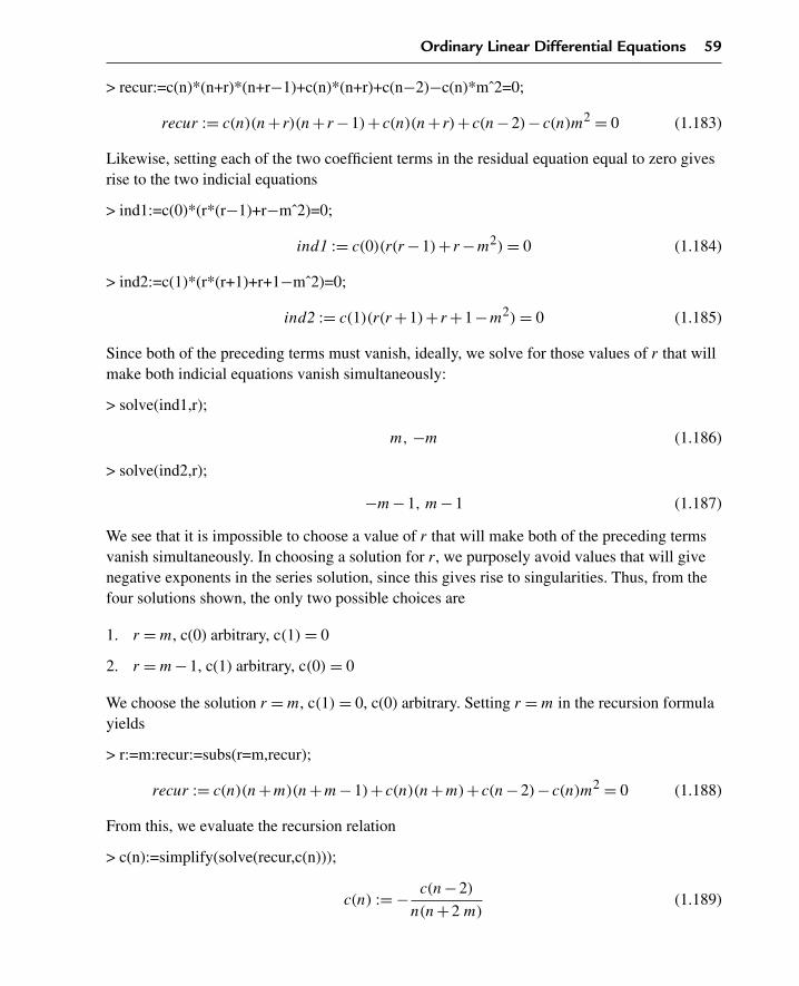
Ordinary Linear Differential Equations 59
> recur:=c(n)*(n+r)*(n+r−1)+c(n)*(n+r)+c(n−2)−c(n)*mˆ2=0;
recur := c(n)(n+ r)(n+ r −1)+ c(n)(n+ r)+ c(n−2)− c(n)m2 = 0 (1.183)
Likewise, setting each of the two coefficient terms in the residual equation equal to zero givesrise to the two indicial equations
> ind1:=c(0)*(r*(r−1)+r−mˆ2)=0;
ind1 := c(0)(r(r −1)+ r −m2) = 0 (1.184)
> ind2:=c(1)*(r*(r+1)+r+1−mˆ2)=0;
ind2 := c(1)(r(r +1)+ r +1−m2) = 0 (1.185)
Since both of the preceding terms must vanish, ideally, we solve for those values of r that willmake both indicial equations vanish simultaneously:
> solve(ind1,r);
m, −m (1.186)
> solve(ind2,r);
−m−1, m−1 (1.187)
We see that it is impossible to choose a value of r that will make both of the preceding termsvanish simultaneously. In choosing a solution for r, we purposely avoid values that will givenegative exponents in the series solution, since this gives rise to singularities. Thus, from thefour solutions shown, the only two possible choices are
1. r = m, c(0) arbitrary, c(1) = 0
2. r = m−1, c(1) arbitrary, c(0) = 0
We choose the solution r = m, c(1) = 0, c(0) arbitrary. Setting r = m in the recursion formulayields
> r:=m:recur:=subs(r=m,recur);
recur := c(n)(n+m)(n+m−1)+ c(n)(n+m)+ c(n−2)− c(n)m2 = 0 (1.188)
From this, we evaluate the recursion relation
> c(n):=simplify(solve(recur,c(n)));
c(n) := − c(n−2)
n(n+2 m)(1.189)
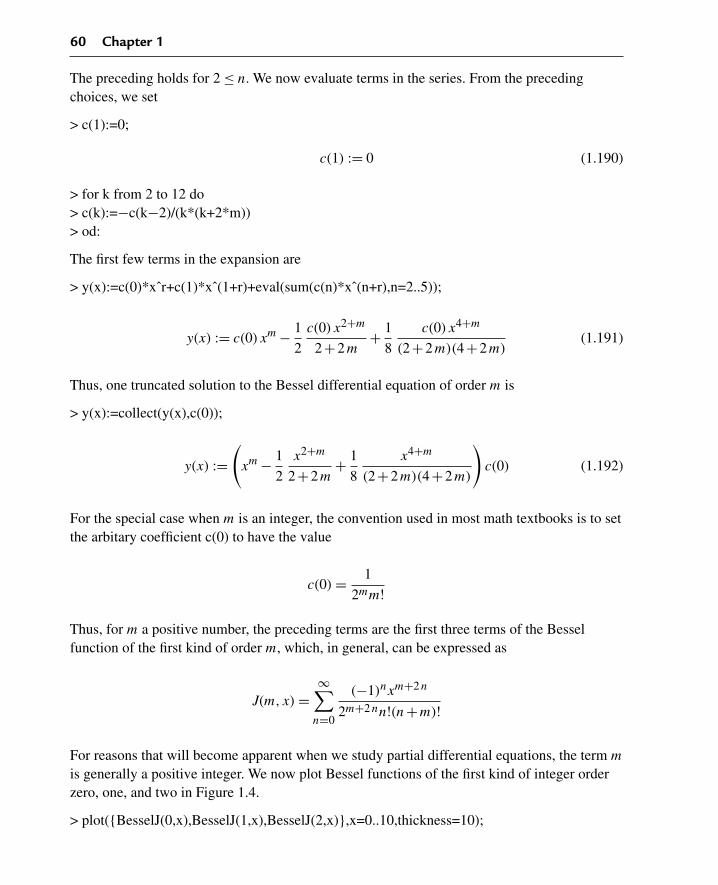
60 Chapter 1
The preceding holds for 2 ≤ n. We now evaluate terms in the series. From the precedingchoices, we set
> c(1):=0;
c(1) := 0 (1.190)
> for k from 2 to 12 do> c(k):=−c(k−2)/(k*(k+2*m))> od:
The first few terms in the expansion are
> y(x):=c(0)*xˆr+c(1)*xˆ(1+r)+eval(sum(c(n)*xˆ(n+r),n=2..5));
y(x) := c(0) xm − 1
2
c(0) x2+m
2+2m+ 1
8
c(0) x4+m
(2+2m)(4+2m)(1.191)
Thus, one truncated solution to the Bessel differential equation of order m is
> y(x):=collect(y(x),c(0));
y(x) :=(
xm − 1
2
x2+m
2+2m+ 1
8
x4+m
(2+2m)(4+2m)
)c(0) (1.192)
For the special case when m is an integer, the convention used in most math textbooks is to setthe arbitary coefficient c(0) to have the value
c(0) = 1
2mm!
Thus, for m a positive number, the preceding terms are the first three terms of the Besselfunction of the first kind of order m, which, in general, can be expressed as
J(m,x) =∞∑
n=0
(−1)nxm+2n
2m+2nn!(n+m)!
For reasons that will become apparent when we study partial differential equations, the term m
is generally a positive integer. We now plot Bessel functions of the first kind of integer orderzero, one, and two in Figure 1.4.
> plot({BesselJ(0,x),BesselJ(1,x),BesselJ(2,x)},x=0..10,thickness=10);

Ordinary Linear Differential Equations 61
x2 6 10
20.4
20.2
0
0.2
0.4
0.6
0.8
1.0
4 8
Figure 1.4
EXAMPLE 1.11.2: Now that we have one solution to the Bessel differential equation of orderm, we seek a second basis vector using the method of reduction of order. For illustrationpurposes and ease of calculation here, we focus on the special case for m = 0, and we consideronly the first three terms in the series expansion of the first basis vector y1(x).
SOLUTION: From Section 1.6, with knowledge of one solution vector y1(x), a second basisvector y2(x) can be found from the equation
y2(x) = y1(x)
⎛⎜⎝∫
e−
(∫a1(x)a2(x)
dx)
y1(x)2dx
⎞⎟⎠
For the Bessel differential equation, we identify the coefficients
> restart: a2(x):=xˆ2;a1(x):=x;
a2(x) := x2 (1.193)
a1(x) := x
The first few terms for y1(x) for m = 0 are
> y1(x):=1−xˆ2/4+xˆ4/64;
y1(x) := 1− 1
4x2 + 1
64x4 (1.194)
Evaluation of the preceding integrand gives
> v(x):=(1/y1(x)ˆ2)*exp(−int(a1(x)/a2(x),x));
v(x) := 1(1− 1
4x2 + 1
64x4
)2x
(1.195)

62 Chapter 1
Taking just the first three terms of the preceding integrand and integrating yields
> u(x):=int(convert(series(v(x),x,3),polynom),x);
u(x) := ln(x)+ 1
4x2 (1.196)
Thus, our truncated series expansion of the second basis vector y2(x) becomes
> y2(x):=simplify(expand(y1(x)*u(x)));
y2(x) := ln(x)+ 1
4x2 − 1
4x2 ln(x)− 1
16x4 + 1
64x4 ln(x)+ 1
256x6 (1.197)
If we compare this second linearly independent solution with Y0(x), the Bessel function of thesecond kind of order m = 0, we have
> Y[0](x):=expand((Pi/2)*(convert(series(BesselY(0,x),x,5),polynom)));
Y0(x) :=− ln(2)+ ln(x)+γ + 1
4x2 ln(2)− 1
4x2 ln(x)+ 1
4x2 − 1
4x2γ − 1
64x4 ln(2)
+ 1
64x4 ln(x)− 3
128x4 + 1
64x4γ (1.198)
Except for the conventions used in establishing certain constants (γ = Euler’s constant), wesee that our second series solution for y2(x) is equivalent to the Bessel function of the secondkind of order zero. Because x = 0 is a regular singular point of the differential equation, wenote that the preceding function fails to exist at the point x = 0.
We plot Bessel functions of the second kind of integer orders zero, one, and two in Figure 1.5.
> plot({BesselY(0,x),BesselY(1,x),BesselY(2,x)},x=0..8,y=−4..2,thickness=10);
x1 3 4 8
y
24
23
22
21
0
1
2
2 5 6 7
Figure 1.5
The significant feature of the plot of Figure 1.5 shows that the Bessel functions of the secondkind, of integer order, all fail to exist at x = 0. The preceding system basis vectors will play a

Ordinary Linear Differential Equations 63
significant role when we consider partial differential equations in the cylindrical coordinatesystem.
Chapter Summary
First-order linear nonhomogeneous differential equation
a1(t)
(d
dty(t)
)+a0(t)y(t) = f(t)
System basis vector
y1(t) = e∫ (
− a0(t)a1(t)
)dt
Particular solution
yp(t) =t∫
0
G1(t, s)f(s)ds
First-order Green’s function G1(t, s)
G1(t, s) = y1(t)
a1(s)y1(s)
Second-order linear nonhomogeneous differential equation
a2(t)
(d2
dt2y(t)
)+a1(t)
(d
dty(t)
)+a0(t)y(t) = f(t)
Second basis vector y2(t) as evaluated from the first y1(t)
y2(t) = y1(t)
⎛⎜⎝∫
e−
(∫a1(s)a2(s)
ds)
y1(s)2ds
⎞⎟⎠
Particular solution in terms of the second-order Green’s function
yp(t) =t∫
0
G2(t, s)f(s)ds
Second-order Green’s function G2(t, s)
G2(t, s) = y1(s)y2(t)−y1(t)y2(s)
a2(s)W(y1(s), y2(s))

64 Chapter 1
Series solution to the second-order linear ordinary differential equation
a2(x)
(d2
dx2y(x)
)+a1(x)
(d
dxy(x)
)+a0(x)y(x) = 0
Assumed Frobenius solution about the origin
y(x) =∞∑
n=0
c(n)xn+r
Equivalent series equation
∞∑n=0
(a2(x)c(n)(n+ r)(n+ r −1)xn+r−2 +a1(x)c(n)(n+ r)xn+r−1 +a0(x)c(n)xn+r
)= 0
From the preceding series equation, we develop the indicial equations and the recursionformula for the final solution.
Most often occurring differential equations
1. The Euler differential equation
d2
dx2y(x)+λy(x) = 0
A set of basis vectors for the Euler equation
y1(x) = sin(√
λx)
and
y2(x) = cos(√
λx)
2. The Cauchy-Euler differential equation
x2
(d2
dx2y(x)
)+x
(d
dxy(x)
)+λy(x) = 0
A set of basis vectors for the Cauchy-Euler equation
y1(x) = sin(√
λ ln(x))
and
y2(x) = cos(√
λ ln(x))

Ordinary Linear Differential Equations 65
3. The Bessel differential equation of order m
x2
(d2
dx2y(x)
)+x
(d
dxy(x)
)+
(x2 −m2
)y(x) = 0
A set of basis vectors for the Bessel equation
y1(x) = J(m,x)
and
y2(x) = Y(m,x)
These procedures have shown that we can find the general solution to both first- andsecond-order linear ordinary nonhomogeneous differential equations. For the case ofsecond-order nonhomogeneous differential equations, we demonstrated that from theknowledge of only a single basis vector, we were able to generate the complete solutionto the differential equation. We have stressed the procedure of the method of variation ofparameters and the subsequent evaluation of the corresponding Green’s function. Thesesolutions will play a big role in the development of solutions to some partial differentialequations later.
Exercises
Consider the following first-order linear nonhomogeneous differential equations. In all cases,evaluate one basis vector y1(x) and the first-order Green’s function G1(x, s), and then writeout the general solution. When possible, use the Maple command dsolve to verify the solution.
1.1.
d
dxy(x)+ y(x)
x= 2+x2
1.2.
x
(d
dxy(x)
)+2y(x) = ex + ln(x)
1.3. (x2 +1
)(d
dxy(x)
)−2xy(x) = x2 +1
1.4.
d
dxy(x)+ tan(x)y(x) = sec(x)

66 Chapter 1
1.5.
x
(d
dxy(x)
)+ (1+x)y(x) = 3 e−x
Consider the following initial-value problems. In all cases, evaluate one basis vector y1(t) andthe first-order Green’s function G1(t, s), and then evaluate the final solution.
1.6. y(0) = 4
d
dty(t)+2y(t) = t + sin(t)
1.7. y(0) = 3
d
dty(t)+ ty(t) = t3
1.8. y(0) = −5
d
dty(t)+ 4y(t)
t +2= 3
1.9. y(0) = 7 (2 t2 +1
)(d
dty(t)
)−10ty(t) = 4 t
1.10. y(0) = 1
d
dty(t)+y(t) = e−2 t
The following problems demonstrate applications of first-order initial value problems.Generate all solutions and develop a graph of the solution and an animated display as done inthe examples in Section 1.3.
1.11. A tank is initially filled with 40 gal of a salt solution containing 2 lb of salt per gal.Fresh brine containing 3 lb of salt per gal runs into the tank at 4 gal per min, and themixture is kept uniform by constant stirring. (a) If the mixture runs out of the tank at thesame rate it runs in, find the amount of salt q(t) at any time in the tank. (b) Evaluate thetime at which the amount of salt in the tank reaches 100 lb. Hint: This is an initial valueproblem with q(0) = 80 lb, and the differential equation is
d
dtq(t) = 12− q(t)
10
1.12. Solve Exercise 1.11 for the case where the initial concentration of salt in the containeris 5 lb of salt per gal.

Ordinary Linear Differential Equations 67
1.13. According to Newton’s law of cooling, a body loses heat at a rate proportional to theinstantaneous temperature difference between the body and its surroundings. Consider abody that loses heat in accordance with this law, where the initial temperature of thebody is 70°C, the surrounding temperature is 20°C, and the temperature decaycoefficient is k = 3/10 per min. (a) Find an expression for the temperature T(t) at anytime t. (b) At what time will the body temperature be 30°C? Hint: This is an initialcondition problem with T(0) = 70°C, and the differential equation is
d
dtT(t) = −k(T(t)−20)
1.14. Solve Exercise 1.13 for the case where k = 5/10/min and T(0) = 100°C.
1.15. A body of mass m undergoes freefall due to gravity in a viscous medium, where theviscous force is proportional to the body speed. We would like to calculate the speedv(t) of a body whose mass is m = 5 kg in freefall if its initial speed is 50 m/sec upwardand the damping coefficient is γ = 1 N/m/sec. The acceleration due to gravity isg = 9.8 m/sec/sec in the MKS system. Hint: This is an initial value problem withv(0) = 50 m/sec, and the differential equation is
m
(d
dtv(t)
)= −mg−γ v(t)
1.16. Solve Exercise 1.15 for the time at which the speed is zero.
1.17. Solve Exercise 1.15 for the case where the damping coefficient is doubled.
1.18. We consider a resistance-inductance (RL) circuit with an impressed voltage e(t), wherethe electric current in the circuit at any time t is i(t). The circuit resistance R = 20 ohmsand the inductance L = 100 henries. At time t = 0, the circuit switch is closed, and theimpressed voltage is e(t) = 20 volts. Solve for the current in the circuit. Hint: This is aninitial value problem with i(0) = 0 amps, and the differential equation is
L
(d
dti(t)
)+Ri(t) = e(t)
1.19. Solve Exercise 1.18 for the case where the impressed voltage is e(t) = 40 sin(t) voltsand the initial current is i(0) = 10 amps.
1.20. We consider a resistance-capacitance (RC) circuit with an impressed voltage e(t), wherethe electric charge on the capacitor at any time t is q(t). The circuit resistance R = 3ohms, and the capacitance C = 2 farads. At time t = 0, the circuit switch is closed andthe capacitor has an initial charge of 200 coulombs. If the impressed voltage ise(t) = 20 volts, solve for the charge in the circuit. Hint: This is an initial value problem

68 Chapter 1
with q(0) = 200 coulombs, and the differential equation is
R
(d
dtq(t)
)+ q(t)
C= e(t)
1.21. Solve Exercise 1.20 where the impressed voltage is e(t) = 10 te−t volts and the initialcharge is q(0) = 0 coulombs. Find the time at which the charge in the circuit is amaximum.
Consider the following second-order linear differential equations with constant coefficients.Evaluate two basis vectors y1(t) and y2(t) and, from these, evaluate the second-order Green’sfunction G2(t, s). With the Green’s function, evaluate a particular solution. When possible, usethe Maple dsolve command to verify the solution.
1.22.
d2
dt2y(t)+4
(d
dty(t)
)+3y(t) = 3et
1.23.
d2
dt2y(t)−5
(d
dty(t)
)+4y(t) = 10 sinh(t)
1.24.
d2
dt2y(t)+2
(d
dty(t)
)−3y(t) = 2+3et
1.25.
d2
dt2y(t)+4
(d
dty(t)
)+13y(t) = sin(t)
Consider the following Cauchy-Euler second-order differential equations with variablecoefficients. Evaluate two basis vectors y1(t) and y2(t) and, from these, evaluate thesecond-order Green’s function G2(t, s).
1.26.
t2
(d2
dt2y(t)
)+7t
(d
dty(t)
)+9y(t) = f(t)
1.27.
t2
(d2
dt2y(t)
)+ t
(d
dty(t)
)+y(t) = f(t)

Ordinary Linear Differential Equations 69
1.28.
t2
(d2
dt2y(t)
)−4t
(d
dty(t)
)+6y(t) = f(t)
1.29.
2t2
(d2
dt2y(t)
)+5t
(d
dty(t)
)+y(t) = f(t)
1.30. In Exercise 1.26, let f(t) = ln(t). Use the evaluated Green’s function to find a particularsolution. Use the Maple dsolve command to verify the solution.
1.31. In Exercise 1.27, let f(t) = t. Use the evaluated Green’s function to find a particularsolution. Use the Maple dsolve command to verify the solution.
1.32. In Exercise 1.28, let f(t) = t4et . Use the evaluated Green’s function to find a particularsolution. Use the Maple dsolve command to verify the solution.
1.33. In Exercise 1.29, let f(t) = t2 − t. Use the evaluated Green’s function to find aparticular solution. Use the Maple dsolve command to verify the solution.
1.34. The simple spring-mass system consists of a mass m that is attached to an ideal springwith a spring constant k. The system is immersed in a viscous damping medium whereγ is the damping coefficient. The external applied force acting on the system is denotedf(t), and the displacement of the mass from its equilibrium position is denoted y(t). Thedifferential equation that describes the system is
m
(d2
dt2y(t)
)+γ
(d
dty(t)
)+ky(t) = f(t)
We look at the case where m = 1 kg, γ = 0 N/m/sec, and k = 9 N/m. (a) Evaluate a setof system basis vectors y1(t) and y2(t), and evaluate the second-order Green’s functionG2(t, s). (b) If the initial conditions are y(0) = 2 m, v(0) = 10 m/sec, and the drivingforce is f(t) = 10 sin(t) N, evaluate the time-dependent solution y(t) for the problem.(c) Graph the solution and develop the animation as done in Example 1.8.1. This is asimple second-order initial value problem.
1.35. Do Exercise 1.34 for the case where m = 1 kg, γ = 1 N/m/sec, k = 37/4 N/m, and thedriving force is f(t) = 20 te−t N. All other conditions are the same. Develop allgraphics and animation.
1.36. Do Exercise 1.34 for the case where m = 1 kg, γ = 1 N/m/sec, k = 82/4 N/m, and thedriving force is f(t) = 10 Heaviside(t) N. [Note: Heaviside(t) denotes the unit stepfunction.] Develop all graphics and animation.
70 Chapter 1
1.37. The series RLC circuit consists of a resistor R, an inductor L, and a capacitor C
connected in series. If the electric charge on the capacitor in the system is denoted asq(t), and the driving voltage is e(t), then the differential equation that describes the timedependence of the charge is given as
L
(d2
dt2q(t)
)+R
(d
dtq(t)
)+ q(t)
C= e(t) (1.199)
We consider the case where L = 1 henry, R = 1 ohms, and C = 4/50 farads and thedriving voltage is e(t) = 10 te−t volts. (a) Evaluate the system basis vectors q1(t) andq2(t) and the second-order Green’s function G2(t, s). (b) If the initial charge q(0) = 0coulombs and the initial current i(0) = 0 amps, evaluate the time dependence of thecharge q(t) on the capacitor. (c) Graph the solution and develop the animation as donein Example 1.8.1. This is a simple second-order initial value problem.
1.38. Do Exercise 1.37 for the case where L = 1 henry, R = 1 ohms, and C = 4/10 farads,and the driving voltage is e(t) = 10 sin(t) volts. All other conditions are the same.Develop all graphics and animation.
For the following differential equations, you are given one basis vector y1(t). You are asked toevaluate a second basis vector y2(t) using the method of reduction of order. You are then askedto evaluate the second-order Green’s function G2(t, s).
1.39. Given one basis vector y1(t) = e3 t , find the second-order Green’s function G2(t, s).
d2
dt2y(t)−6
(d
dty(t)
)+9y(t) = f(t)
1.40. Given one basis vector y1(t) = t, find the second-order Green’s function G2(t, s).
t2
(d2
dt2y(t)
)− t
(d
dty(t)
)+y(t) = f(t)
1.41. Given one basis vector y1(t) = t −1, find the second-order Green’s function G2(t, s).
(2 t − t2
)(d2
dt2y(t)
)+2(t −1)
(d
dty(t)
)−2y(t) = f(t)
1.42. Given one basis vector y1(t) = t3, find the second-order Green’s function G2(t, s).
t2
(d2
dt2y(t)
)−6y(t) = f(t)

Ordinary Linear Differential Equations 71
1.43. Given one basis vector y1(t) = t, find the second-order Green’s function G2(t, s).
t3
(d2
dt2y(t)
)+ t
(d
dty(t)
)−y(t) = f(t) (1.200)
1.44. Let f(t) = te3 t in Exercise 1.39. Use the Green’s function that you evaluated to find aparticular solution. Check your answer by substituting the solution back into thedifferential equation.
1.45. Let f(t) = 1t in Exercise 1.40. Use the Green’s function that you evaluated to find a
particular solution. Use the Maple dsolve command to verify the solution.
1.46. Let f(t) = t3 ln(t) in Exercise 1.42. Use the Green’s function that you evaluated to finda particular solution. Use the Maple dsolve command to verify the solution.
1.47. Let f(t) = t in Exercise 1.43. Use the Green’s function that you evaluated to find aparticular solution. Use the Maple dsolve command to verify the solution.
The following linear differential equations are to be solved by using the method of Frobeniusfor finding a series solution about the origin (x = 0). For the Exercises 1.48 through 1.51,(a) evaluate the indicial equations and the corresponding recursion formula. (b) From theindicial equation, obtain a set of basis vectors from different choices of roots of the indicialequation. If you are able to obtain only one solution, then use the method of reduction of orderto find a second basis vector.
1.48.
d2
dx2y(x)+x
(d
dxy(x)
)+y(x) = 0
1.49.
d2
dx2y(x)−x
(d
dxy(x)
)−x2y(x) = 0
1.50.
x
(d2
dx2y(x)
)+2
(d
dxy(x)
)+xy(x) = 0
1.51.
x
(d2
dx2y(x)
)+3
(d
dxy(x)
)−y(x) = 0

72 Chapter 1
1.52. The Bessel differential equation solved in Section 1.11 comes about when oneconsiders the diffusion and wave equations in the cylindrical coordinate system. For aninteger m, the Bessel function of the first kind of order m reads as
J(m,x) =∞∑
n=0
(−1)nxm+2n
2m+2nn!(m+n)!From the preceding series, verify the following(a)
J(0,0) = 1
(b)
J(0,−x) = J(0, x)(c)
d
dxJ(0, x) = −J(1, x)
(d)
x
(∂
∂xJ(m,x)
)= −mJ(m,x)+xJ(m−1, x)
(e) ∫xmJ(m−1, x)dx = xmJ(m,x)
(f)
2mJ(m,x) = x(J(m−1, x)+J(m+1, x))
CHAPTER 2
Sturm-Liouville EigenvalueProblems and Generalized
Fourier Series
2.1 Introduction
In Chapter 1 we examined both first- and second-order linear homogeneous andnonhomogeneous differential equations. We established the significance of the dimension ofthe solution space and the basis vectors. With a set of basis vectors, we could span the entiresolution space of the homogeneous equation by way of a linear superposition of these basisvectors. We also showed how the method of variation of parameters utilized the basisvectors in the construction of the Green’s function. With the Green’s function in hand, wewere then able to evaluate the solution to the corresponding nonhomogeneous differentialequation.
2.2 The Regular Sturm-Liouville Eigenvalue Problem
We will now focus on second-order differential equations, over finite intervals, when theindependent variable is the spatial variable x. These problems will play a prominent role inthe type of partial differential equations that we will look at later.
The problems that we examine here fall under the general category of what are called “regular”Sturm-Liouville eigenvalue problems. These are basically second-order linear homogeneousdifferential equations whose constraints are in the form of two-point, homogeneous, nonmixedboundary conditions.
To begin, we first define the generalized Sturm-Liouville differential operator L acting onsome function y(x) over a finite interval I = {x |a < x < b} as follows:
L(y) = D(p(x)D(y))+q(x)y (2.1)
© 2009, 2003, 1999 Elsevier Inc. 73

74 Chapter 2
Here, D is the standard differentiation operator defined as
D(y) = d
dxy(x)
The “regular” Sturm-Liouville eigenvalue problem consists of two parts:
1. The homogeneous Sturm-Liouville differential equation
L(ϕ)+λw(x)ϕ = 0
2. The “regular” boundary conditions that are homogeneous, nonmixed (single point,spatially separated) conditions at the end points
κ1ϕ(a)+κ2ϕx(a) = 0
and
κ3ϕ(b)+κ4ϕx(b) = 0
The coefficients κ1, κ2, κ3, κ4 are all real constants. Restrictive conditions on the system arethat over the finite interval I, the functions p(x), p′(x), q(x), and w(x) are real continuousfunctions and that p(x) and w(x) are positive over this interval I. In some situations, thepreceding conditions can be relaxed and modified somewhat and the problem becomes“singular.” We shall consider singular problems later.
The Sturm-Liouville differential equation given earlier is linear and homogeneous, and theboundary conditions are homogeneous and nonmixed. The allowed values of λn for which thepreceding differential equation satisfies the boundary conditions are called the “eigenvalues,”and the corresponding solutions ϕn(x) are called the “eigenfunctions.”
We state, without proof, some of the important features of “regular” Sturm-Liouville problems:
1. There exist an infinite number of eigenvalues λn that can be ordered in magnitude and thatcan be indexed by the positive integers n = 0,1,2,3, . . . .
2. All eigenvalues are real.
3. Corresponding to each eigenvalue λn there exists a unique eigenfunction ϕn(x).
4. The eigenfunctions form a “complete” set with respect to any piecewise smooth functionf(x) over the finite interval I = {x |a < x < b}. This means that, over this interval, thefunction can be represented as a generalized Fourier series expansion in terms of theeigenfunctions shown here:
f(x) =∞∑
n=0
F(n)ϕn(x)
where the terms F(n) are the properly evaluated Fourier coefficients.

Sturm-Liouville Eigenvalue Problems and Generalized Fourier Series 75
5. The infinite series given converges to the average of the left- and right-hand limits of thefunction at any point in the interval; that is,
∞∑n=0
F(n)ϕn(x) = f(x+0)+f(x−0)
2
6. The eigenfunctions corresponding to different eigenvalues are orthogonal relative to the“weight function” w(x) over the interval I. If the orthogonal eigenfunctions are furthernormalized, then we can express the statement of orthonormality of the eigenfunctions interms of the inner product (see Chapter 0), with respect to the weight function w(x), as
b∫a
ϕn(x)ϕm(x)w(x)dx = δ(n,m)
where we have used the Kronecker delta function δn,m, which, by definition, has the value1 for n = m and the value 0 for n �= m.
2.3 Green’s Formula and the Statement of Orthonormality
In terms of the standard differentiation operator D, the Sturm-Liouville operator L acting onsome function y(x) reads
L(y) = D(p(x)D(y))+q(x)y
It should be remarked that any second-order linear differential operator
a2(x)D2 +a1(x)D+a0(x)
can be written in Sturm-Liouville form (see Exercise 2.1) by multiplying the operator by theintegrating factor
r(x) = e
∫a1(x)a2(x)
dx
a2(x)
We now provide a formal proof of the statement of orthogonality of the eigenfunctions. Weconsider the Sturm-Liouville operator acting on the two different functions u and v:
L(u) = D(p(x)D(u))+q(x)u
and
L(v) = D(p(x)D(v))+q(x)v
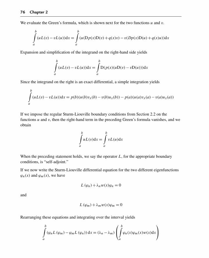
76 Chapter 2
We evaluate the Green’s formula, which is shown next for the two functions u and v.
b∫a
(uL(v)−vL(u))dx =b∫
a
(u(Dp(x)D(v)+q(x)v)−v(Dp(x)D(u)+q(x)u))dx
Expansion and simplification of the integrand on the right-hand side yields
b∫a
(uL(v)−vL(u))dx =b∫
a
D(p(x)(uD(v)−vD(u)))dx
Since the integrand on the right is an exact differential, a simple integration yields
b∫a
(uL(v)−vL(u))dx = p(b)(u(b)vx(b)−v(b)ux(b))−p(a)(u(a)vx(a)−v(a)ux(a))
If we impose the regular Sturm-Liouville boundary conditions from Section 2.2 on thefunctions u and v, then the right-hand term in the preceding Green’s formula vanishes, and weobtain
b∫a
uL(v)dx =b∫
a
vL(u)dx
When the preceding statement holds, we say the operator L, for the appropriate boundaryconditions, is “self-adjoint.”
If we now write the Sturm-Liouville differential equation for the two different eigenfunctionsϕn(x) and ϕm(x), we have
L(ϕn)+λnw(x)ϕn = 0
and
L(ϕm)+λmw(x)ϕm = 0
Rearranging these equations and integrating over the interval yields
b∫a
(ϕnL(ϕm)−ϕmL(ϕn))dx = (λn −λm)
⎛⎝ b∫
a
ϕn(x)ϕm(x)w(x)dx
⎞⎠

Sturm-Liouville Eigenvalue Problems and Generalized Fourier Series 77
If the eigenfunctions satisfy the regular Sturm-Liouville boundary conditions from Section 2.2,then Green’s formula shows the left-hand side to be zero and, thus, the right-hand side is alsozero. This yields the statement of orthogonality of the eigenfunctions:
(λn −λm)
⎛⎝ b∫
a
ϕn(x)ϕm(x)w(x)dx
⎞⎠ =0
The integral here denotes the inner product (see Chapter 0) of the two different eigenfunctionswith respect to the weight function w(x) over the interval I = {x |a < x < b}. This result showsthat if the eigenvalues are not equal—that is, λn �= λm—then the eigenfunctions,corresponding to the different eigenvalues, are orthogonal with respect to the weight functionw(x) over the interval I.
The Statement of Orthonormality
To normalize a vector, we simply divide the vector by its length or norm. From Chapter 0,recall that the norm is the square root of the inner product of the vector with itself with respectto the weight function w(x)—that is,
norm =
√√√√√ b∫a
ϕn(x)2w(x)dx
If we normalize the eigenfunctions—that is, divide each by its length (norm)—then thepreceding condition of orthogonality yields an equivalent “statement of orthonormality,”which, in terms of the Kronecker delta function, reads
b∫a
ϕn(x)ϕm(x)w(x)dx = δ(n,m) (2.2)
This statement indicates the two different eigenfunctions to be orthonormal (a combinationof being orthogonal and normalized) with respect to the weight function w(x) over theinterval I. This result will play a significant role in the development of the generalized Fourierseries.
Types of Boundary Conditions
Before we consider different examples of Sturm-Liouville operators with various types ofnonmixed homogeneous boundary conditions, we first classify the regular boundary conditionsthat we will look at in three types. Let point a be the boundary point.

78 Chapter 2
1. Type 1 or Dirichlet condition (vanishing of the zero derivative at the boundary)
y(a) = 0
2. Type 2 or Neumann condition (vanishing of the first derivative at the boundary)
yx(a) = 0
3. Type 3 or Robin condition (linear dependence between zero and first derivative atboundary)
yx(a)+hy(a) = 0
The constant h in the Robin condition has the dimension of the reciprocal of displacement.When we consider actual boundary value problems, we will be able to attach physicalsignificance to each of these conditions. We now provide an illustration of a typicalSturm-Liouville eigenvalue problem.
DEMONSTRATION: We seek the eigenvalues and corresponding eigenfunctions for theEuler differential equation shown:
d2
dx2y(x)+λy(x) = 0
over the interval I = {x |0 < x < 1} with the boundary conditions
yx(0) = 0
and
y(1) = 0
From our earlier classification of boundary conditions, we have a type 2 condition at the leftand a type 1 condition at the right.
By comparison, we see the Euler differential equation to be a special case of a Sturm-Liouvilledifferential equation
L(y)+λw(x)y = 0
where L is the Sturm-Liouville operator
L(y) = D(p(x)D(y))+q(x)y
For the Euler differential equation, we identify the coefficients p(x) = 1, q(x) = 0, andw(x) = 1.

Sturm-Liouville Eigenvalue Problems and Generalized Fourier Series 79
SOLUTION: To solve for the eigenvalues, we consider three possible cases for values of λ.We first consider the case for λ < 0. We set λ = −μ2. From Chapter 1, a set of basis vectorsfor this case is
y1(x) = sinh(μx)
and
y2(x) = cosh(μx)
and the general solution can be written in terms of this basis as
y(x) = C1 sinh(μx)+C2 cosh(μx)
Substituting the boundary conditions at x = 0 and at x = 1, we get
C1μ = 0
and
C2μ sinh(1) = 0
The only solution to the preceding is the trivial solution C1 = 0 and C2 = 0.
We next consider the case for λ = 0. A set of system basis vectors is
y1(x) = 1
and
y2(x) = x
and the general solution in terms of this basis is
y(x) = C1+C2x
Substituting the boundary condition at x = 0 and at x = 1 gives
C2 = 0
and
C1+C2 = 0
The only solution to the preceding is the trivial solution C1 = 0 and C2 = 0. From a geometricstandpoint, we expected this result because it is impossible to have a nontrivial line that willsatisfy the boundary conditions at both the left and right end points of the interval.

80 Chapter 2
Finally, we consider the case for λ > 0. We set λ = μ2. From Chapter 1, a set of basis vectorsfor this case is
y1(x) = sin(μx)
and
y2(x) = cos(μx)
The general solution here is
y(x) = C1 sin(μx)+C2 cos(μx)
Substituting the boundary conditions at x = 0 and at x = 1, we get
C1μ = 0
and
C1 sin(μ)+C2 cos(μ) = 0
The only nontrivial solutions to the preceding are that C1 = 0, C2 is arbitrary, and μ has valuesthat are the roots of the eigenvalue equation
cos(μ) = 0
Thus, μ takes on the special values
μn = (2n−1)π
2
for n = 1,2,3, . . . .
The allowed eigenvalues λn = μ2n are
λn = (2n−1)2π2
4
and the corresponding eigenfunctions are
ϕn(x) = cos
((2n−1)πx
2
)
for n = 1,2,3, . . . .
These eigenfunctions are not normalized. We must first find the norm of each eigenfunction byevaluating the square root of the inner product of the eigenfunctions with respect to the weightfunction w(x) = 1 over the interval.

Sturm-Liouville Eigenvalue Problems and Generalized Fourier Series 81
The norm is
norm =
√√√√√1∫
0
cos
((2n−1)πx
2
)2dx
Evaluating this integral yields
norm =√
2
2
Dividing each eigenfunction by its norm yields the orthonormal set of eigenfunctions
ϕn(x) = √2 cos
((2n−1)πx
2
)
for n = 1,2,3, . . . .
The statement of orthonormality for this set of eigenfunctions reads
1∫0
2 cos
((2n−1)πx
2
)cos
((2m−1)πx
2
)dx = δ(n,m)
for n,m = 1,2,3, . . . .
2.4 The Generalized Fourier Series Expansion
Since the eigenfunctions form a “complete” set with respect to any piecewise smooth functionf(x) over the interval I = {x |a < x < b}, then we can expand f(x) as a generalized Fourierseries. In terms of the orthonormalized eigenfunctions, the generalized expansion formula forf(x) reads
f(x) =∞∑
n=0
F(n)ϕn(x)
where the F (n) are the generalized Fourier coefficients of the function f(x). We proceed toevaluate these coefficients in a formal manner by taking advantage of the statement oforthonormality given earlier.
If we take the inner product of both sides of the preceding equation, with respect to the weightfunction w(x) over the interval, and we assume it is valid to interchange the order of thesummation and integration operators (see exercises on conditions for this), then we get
b∫a
f(x)ϕm(x)w(x)dx =∞∑
n=0
F(n)
⎛⎝ b∫
a
ϕn(x)ϕm(x)w(x)dx
⎞⎠
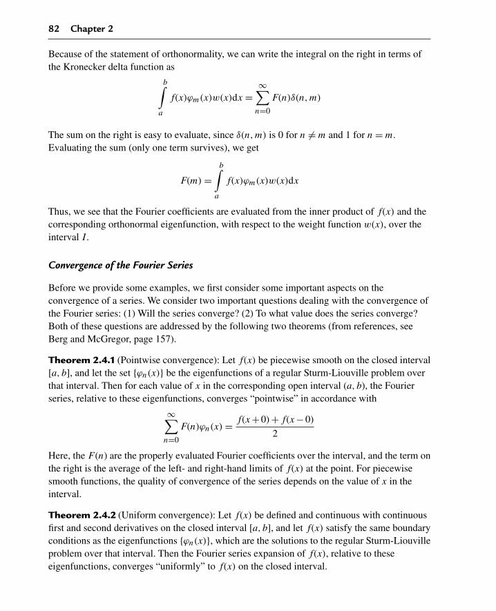
82 Chapter 2
Because of the statement of orthonormality, we can write the integral on the right in terms ofthe Kronecker delta function as
b∫a
f(x)ϕm(x)w(x)dx =∞∑
n=0
F(n)δ(n,m)
The sum on the right is easy to evaluate, since δ(n,m) is 0 for n �= m and 1 for n = m.Evaluating the sum (only one term survives), we get
F(m) =b∫
a
f(x)ϕm(x)w(x)dx
Thus, we see that the Fourier coefficients are evaluated from the inner product of f(x) and thecorresponding orthonormal eigenfunction, with respect to the weight function w(x), over theinterval I.
Convergence of the Fourier Series
Before we provide some examples, we first consider some important aspects on theconvergence of a series. We consider two important questions dealing with the convergence ofthe Fourier series: (1) Will the series converge? (2) To what value does the series converge?Both of these questions are addressed by the following two theorems (from references, seeBerg and McGregor, page 157).
Theorem 2.4.1 (Pointwise convergence): Let f(x) be piecewise smooth on the closed interval[a, b], and let the set {ϕn(x)} be the eigenfunctions of a regular Sturm-Liouville problem overthat interval. Then for each value of x in the corresponding open interval (a, b), the Fourierseries, relative to these eigenfunctions, converges “pointwise” in accordance with
∞∑n=0
F(n)ϕn(x) = f(x+0)+f(x−0)
2
Here, the F (n) are the properly evaluated Fourier coefficients over the interval, and the term onthe right is the average of the left- and right-hand limits of f(x) at the point. For piecewisesmooth functions, the quality of convergence of the series depends on the value of x in theinterval.
Theorem 2.4.2 (Uniform convergence): Let f(x) be defined and continuous with continuousfirst and second derivatives on the closed interval [a, b], and let f(x) satisfy the same boundaryconditions as the eigenfunctions {ϕn(x)}, which are the solutions to the regular Sturm-Liouvilleproblem over that interval. Then the Fourier series expansion of f(x), relative to theseeigenfunctions, converges “uniformly” to f(x) on the closed interval.

Sturm-Liouville Eigenvalue Problems and Generalized Fourier Series 83
Functions that satisfy the more rigid conditions for uniform convergence are more wellbehaved and have Fourier series expansions that converge more rapidly and with better fidelityto the actual function. Uniform convergence obviously implies pointwise convergence at allpoints on the closed interval, and, in addition, the convergence is independent of the value of x
on that interval. For more details on testing a series for uniform convergence, see Section 3.7,which discusses the Weierstrass M-test for the uniform convergence of a series. For moreformal definitions of the concepts of pointwise and uniform convergence, please be advisedthat these concepts are best discussed in more advanced texts in Fourier series (see references).The more advanced concepts of periodic entensions and Gibb’s phenomena are best discussedin these more advanced texts.
We now provide illustrations of Fourier series expansions of three different functions in termsof those eigenfunctions derived in the problem in Section 2.3. This exercise demonstrates howthe quality of convergence of the resulting series depends on the character of the function andhow well it adheres to the boundary conditions on the problem.
DEMONSTRATION: We seek the generalized series expansion of a piecewise smoothfunction f(x) over the interval I = {x |0 < x < 1}, in terms of the orthonormal eigenfunctionsevaluated in Section 2.3.
SOLUTION: In terms of the evaluated orthonormal eigenfunctions, the expansion reads
f(x) =∞∑
n=1
F(n) cos
((2n−1)πx
2
)√2
From the preceding, the Fourier coefficients are determined from the integral
F(n) =1∫
0
f(x) cos
((2n−1)πx
2
)√2 dx
We evaluate the series for three different functions f(x), each having a different character overthe interval.
Case 1 We let f1(x) = x. For this case, f1(x) does not satisfy either of the boundaryconditions at the left or right end points of the interval. The Fourier coefficient integral reads
F(n) =1∫
0
x√
2 cos
((2n−1)πx
2
)dx
Evaluation of this integral yields
F(n) = −2√
2(2π (−1)nn−π (−1)n +2)
(2n−1)2π2(2.3)

84 Chapter 2
Thus, the Fourier series expansion of f1(x) over the interval is
f1(x) =∞∑
n=1
⎛⎝−
4 (2πn(−1)n −π (−1)n +2) cos(
(2n−1)πx2
)(2n−1)2π2
⎞⎠
A plot of both f1(x) and the first five terms of the series expansion is shown in Figure 2.1.
0 0.2 0.4 0.6 0.8 10
0.2
0.4
0.6
0.8
1
Figure 2.1
Because the function f1(x) does not satisfy either of the boundary conditions, the seriesconverges pointwise. The series converges very slowly, as an alternating 1
n series, and thequality of convergence appears to be poor.
Case 2 We let f2(x) = 1−x. For this case, f2(x) does not satisfy the boundary conditionat the left, but it does satisfy the condition at the right end point of the interval. The Fouriercoefficient integral reads
F(n) =1∫
0
(1−x)√
2 cos
((2n−1)πx
2
)dx
Evaluation of this integral yields
F(n) = 4√
2
(2n−1)2π2(2.4)
Thus, the Fourier series expansion of f2(x) over the interval is
f2(x) =∞∑
n=1
8 cos(
(2n−1)πx2
)(2n−1)2π2
A plot of both f2(x) and the first five terms of the series expansion is shown in Figure 2.2.

Sturm-Liouville Eigenvalue Problems and Generalized Fourier Series 85
The function f2(x) satisfies the boundary condition at the right but not at the left end point,and the series converges pointwise. The series converges very rapidly as a 1
n2 series, and, sincethe function satisfies the boundary condition at one of the end points, the quality ofconvergence appears to be much better than that for case 1.
Case 3 We let f3(x) = 1−x2. For this case, f3(x) satisfies both boundary conditons at theleft and right end points of the interval. The Fourier coefficient integral reads
F(n) =1∫
0
(1−x2)√
2 cos
((2n−1)πx
2
)dx
Evaluation of this integral yields
F(n) = 16√
2(−1)n+1
(2n−1)3π2
Thus, the Fourier series expansion of f3(x) over the interval is
f3(x) =∞∑
n=1
32 (−1)n+1 cos(
(2n−1)πx2
)(2n−1)3π2
A plot of both f3(x) and the first five terms of the series expansion is shown in Figure 2.3.
0 0.2 0.4 0.6 0.8 10
0.2
0.4
0.6
0.8
1
Figure 2.2
0 0.2 0.4 0.6 0.8 10
0.2
0.4
0.6
0.8
1
Figure 2.3

86 Chapter 2
Because the function f3(x) satisfies both of the boundary conditions at the left and right endpoints, the series converges uniformly to f(x). The series converges very rapidly as a 1
n3 series,and the quality of convergence is considerably much better than either of the two cases alreadydiscussed.
2.5 Examples of Regular Sturm-Liouville Eigenvalue Problems
We will now look at examples of regular Sturm-Liouville differential equations with variouscombinations of the three types of boundary conditions discussed earlier. All of the examplesare special cases of the Sturm-Liouville differential equation
L(y)+λw(x)y = 0
where L is the Sturm-Liouville operator
L(y) = D(p(x)D(y))+q(x)y
We focus on three types of differential equations: Euler, Cauchy-Euler, and Bessel. Each one ofthese differential equations is characterized by a different set of Sturm-Liouville coefficients:p(x), q(x), and w(x). Subject to a particular set of boundary conditions, we will generate theeigenvalues, the corresponding eigenfunctions, and the statement of orthonormality. We willthen provide an example of a generalized Fourier series expansion of a given function in termsof the particular eigenfunctions.
In solving for the allowed eigenvalues and corresponding eigenfunctions, we would ordinarilyconsider three possibilities for values of λ: λ < 0, λ = 0, and λ > 0. However, to make our taska little simpler, we will not consider the case for λ < 0 because it can be shown, by way of theRayleigh quotient (see Exercises 2.24 through 2.26), that for the particular Sturm-Liouvilleproblems we will be considering, λ must be greater than or equal to zero.
EXAMPLE 2.5.1: Consider the Euler operator with Dirichlet conditions. We seek theeigenvalues and corresponding orthonormal eigenfunctions for the Euler differential equation[Sturm-Liouville type for p(x) = 1, q(x) = 0, w(x) = 1] over the interval I = {x|0 < x < b}.The boundary conditions are type 1 at the left and type 1 at the right end points.
Euler differential equation
d2
dx2y(x)+λy(x) = 0
Boundary conditions
y(0) = 0 and y(b) = 0

Sturm-Liouville Eigenvalue Problems and Generalized Fourier Series 87
SOLUTION: We consider two possibilities for values of λ. We first consider λ = 0. For thiscase, the system basis vectors are
> restart:y1(x):=1;y2(x):=x;
y1(x) := 1
y2(x) := x (2.5)
General solution
> y(x):=C1*y1(x)+C2*y2(x);
y(x) := C1+C2x (2.6)
Substitution into the boundary conditions yields
> eval(subs(x=0,y(x)))=0;
C1 = 0 (2.7)
> eval(subs(x=b,C1=0,y(x)))=0;
C2b = 0 (2.8)
The only solution to the preceding is the trivial solution. We next consider λ > 0. We setλ = μ2 and, for this case, the system basis vectors are
> y1(x):=sin(mu*x);y2(x):=cos(mu*x);
y1(x) := sin(μx)
y2(x) := cos(μx) (2.9)
General solution
> y(x):=C1*y1(x)+C2*y2(x);
y(x) := C1 sin(μx)+C2 cos(μx) (2.10)
Substituting into the boundary conditions, we get
> eval(subs(x=0,y(x)))=0;
C2 = 0 (2.11)
> eval(subs(x=b,y(x)))=0;
C1 sin(μb)+C2 cos(μb) = 0 (2.12)

88 Chapter 2
The only nontrivial solutions to the preceding occur when C2 = 0, C1 is arbitrary, and μ
satisfies the following eigenvalue equation:
> sin(mu*b)=0;
sin(μb) = 0 (2.13)
Thus, μ takes on the values
> mu[n]:=n*Pi/b;
μn := nπ
b(2.14)
for n = 1,2,3, . . . .
Allowed eigenvalues are λn = μ2n
> lambda[n]:=(n*Pi/b)ˆ2;
λn := n2π2
b2(2.15)
Nonnormalized eigenfunctions are
> phi[n](x):=sin(mu[n]*x);
φn(x) := sin(nπx
b
)(2.16)
Normalization
Evaluating the norm from the inner product of the eigenfunctions with respect to the weightfunction w(x) = 1 over the interval yields
> w(x):=1:unprotect(norm):norm:=sqrt(Int(phi[n](x)ˆ2*w(x),x=0..b));norm:=expand(value(%)):
norm :=
√√√√√b∫
0
sin(nπx
b
)2dx (2.17)
Substitution of the eigenvalue equation simplifies the norm
> norm:=radsimp(subs({sin(n*Pi)=0,cos(n*Pi)=(−1)ˆn},norm));
norm := 1
2
√2√
b (2.18)
Orthonormal eigenfunctions

Sturm-Liouville Eigenvalue Problems and Generalized Fourier Series 89
> phi[n](x):=phi[n](x)/norm;phi[m](x):=subs(n=m,phi[n](x)):
φn(x) := sin(nπxb
)√2√
b(2.19)
Statement of orthonormality
> Int(phi[n](x)*phi[m](x)*w(x),x=0..b)=delta(n,m);
b∫0
2 sin(nπxb
)sin
(mπx
b
)b
dx = δ(n,m) (2.20)
Generalized Fourier series expansion
> f(x):=Sum(F(n)*phi[n](x),n=1..infinity);f(x):=‘f(x)’:
f(x) :=∞∑
n=1
F(n) sin(nπxb
)√2√
b(2.21)
Fourier coefficients
> F(n):=Int(f(x)*phi[n](x)*w(x),x=0..b);F(n):=‘F(n)’:
F(n) :=b∫
0
f(x) sin(nπxb
)√2√
bdx (2.22)
This is the generalized series expansion of f(x) in terms of the “complete” set of eigenfunctionsfor the particular Sturm-Liouville operator and given boundary conditions over the interval.
DEMONSTRATION: Develop the generalized series expansion for f(x) = x over the intervalI = {x |0 < x < 1} in terms of the preceding eigenfunctions. We assign the system values
> a:=0;b:=1;f(x):=x;
a := 0
b := 1
f(x) := x (2.23)
SOLUTION: We evaluate the Fourier coefficients
> F(n):=eval(Int(f(x)*phi[n](x)*w(x),x=a..b));F(n):=value(%):
F(n) :=1∫
0
x sin(nπx)√
2dx (2.24)

90 Chapter 2
> F(n):=subs({sin(n*Pi)=0,cos(n*Pi)=(−1)ˆn},F(n));
F(n) := −√
2(−1)n
nπ(2.25)
> Series:=eval(Sum(F(n)*phi[n](x),n=1..infinity));
Series :=∞∑
n=1
(−2(−1)n sin(nπx)
nπ
)(2.26)
First five terms of expansion
> Series:=sum(F(n)*phi[n](x),n=1..5):
x0 0.2 0.4 0.6 0.8 1
0
0.2
0.4
0.6
0.8
1
Figure 2.4
The curves of Figure 2.4 depict the function f(x) and its Fourier series approximation in termsof the orthonormal eigenfunctions for the particular operator and boundary conditions givenearlier. Note that f(x) satisfies the given boundary conditions at the left but fails to do so at theright end point. The convergence is pointwise.
EXAMPLE 2.5.2: Consider the Euler operator with Dirichlet and Neumann conditions. Weseek the eigenvalues and corresponding orthonormal eigenfunctions for the Euler differentialequation [Sturm-Liouville type for p(x) = 1, q(x) = 0, w(x) = 1] over the intervalI = {x |0 < x < b}. The boundary conditions are type 1 at the left and type 2 at the right.
Euler differential equation
d2
dx2y(x)+λy(x) = 0
Boundary conditions
y(0) = 0 and yx(b) = 0
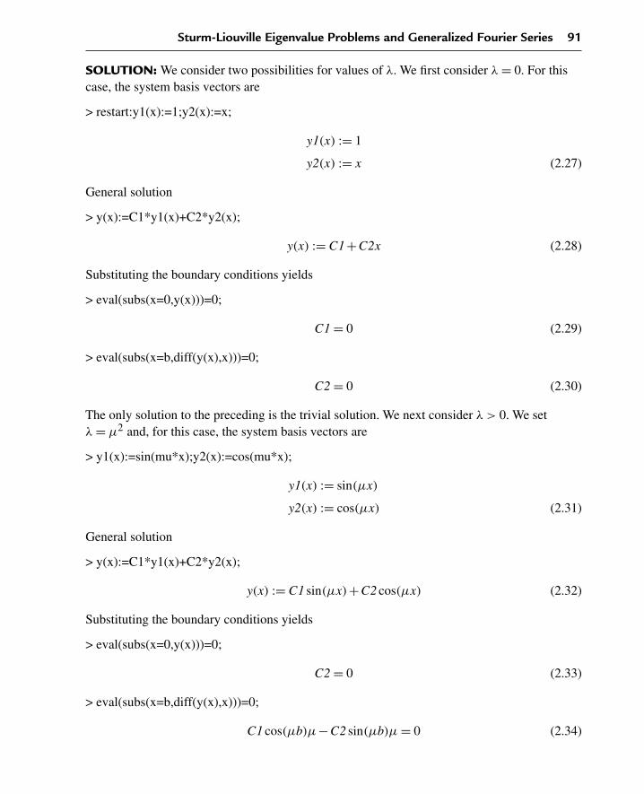
Sturm-Liouville Eigenvalue Problems and Generalized Fourier Series 91
SOLUTION: We consider two possibilities for values of λ. We first consider λ = 0. For thiscase, the system basis vectors are
> restart:y1(x):=1;y2(x):=x;
y1(x) := 1
y2(x) := x (2.27)
General solution
> y(x):=C1*y1(x)+C2*y2(x);
y(x) := C1+C2x (2.28)
Substituting the boundary conditions yields
> eval(subs(x=0,y(x)))=0;
C1 = 0 (2.29)
> eval(subs(x=b,diff(y(x),x)))=0;
C2 = 0 (2.30)
The only solution to the preceding is the trivial solution. We next consider λ > 0. We setλ = μ2 and, for this case, the system basis vectors are
> y1(x):=sin(mu*x);y2(x):=cos(mu*x);
y1(x) := sin(μx)
y2(x) := cos(μx) (2.31)
General solution
> y(x):=C1*y1(x)+C2*y2(x);
y(x) := C1 sin(μx)+C2 cos(μx) (2.32)
Substituting the boundary conditions yields
> eval(subs(x=0,y(x)))=0;
C2 = 0 (2.33)
> eval(subs(x=b,diff(y(x),x)))=0;
C1 cos(μb)μ−C2 sin(μb)μ = 0 (2.34)

92 Chapter 2
The only nontrivial solutions occur when C2 = 0, C1 is arbitrary, and μ satisfies the followingeigenvalue equation:
> cos(mu*b)=0;
cos(μb) = 0 (2.35)
Thus, μ takes on values
> mu[n]:=(2*n−1)*Pi/(2*b);
μn := 1
2
(2n−1)π
b(2.36)
for n = 1,2,3, . . . .
Allowed eigenvalues are λn = μ2n
> lambda[n]:=mu[n]ˆ2;
λn := 1
4
(2n−1)2π2
b2(2.37)
Nonnormalized eigenfunctions are
> phi[n](x):=sin(mu[n]*x);
ϕn(x) := sin
(1
2
(2n−1)πx
b
)(2.38)
Normalization
Evaluating the norm from the inner product of the eigenfunctions with respect to the weightfunction w(x) = 1 over the interval yields
> w(x):=1:unprotect(norm):norm:=sqrt(Int(phi[n](x)ˆ2*w(x),x=0..b));norm:=expand(value(%)):
norm :=
√√√√√b∫
0
sin
(1
2
(2n−1)πx
b
)2dx (2.39)
Substitution of the eigenvalue equation simplifies the norm
> norm:=radsimp(subs({sin(n*Pi)=0,cos(n*Pi)=(−1)ˆn},norm));
norm := 1
2
√2√
b (2.40)
Orthonormal eigenfunctions
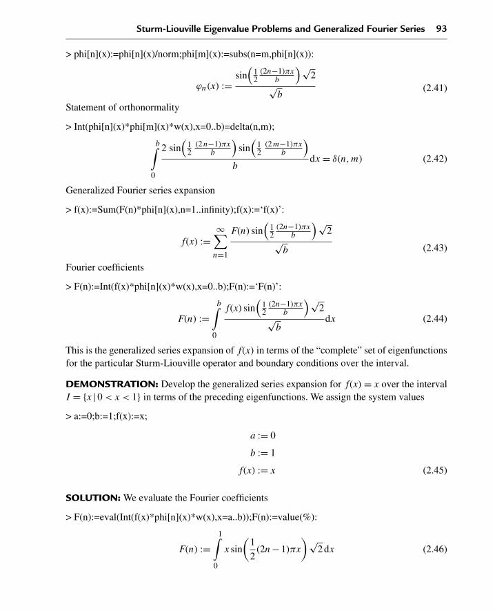
Sturm-Liouville Eigenvalue Problems and Generalized Fourier Series 93
> phi[n](x):=phi[n](x)/norm;phi[m](x):=subs(n=m,phi[n](x)):
ϕn(x) :=sin
(12
(2n−1)πxb
)√2
√b
(2.41)
Statement of orthonormality
> Int(phi[n](x)*phi[m](x)*w(x),x=0..b)=delta(n,m);
b∫0
2 sin(
12
(2n−1)πxb
)sin
(12
(2m−1)πxb
)b
dx = δ(n,m) (2.42)
Generalized Fourier series expansion
> f(x):=Sum(F(n)*phi[n](x),n=1..infinity);f(x):=‘f(x)’:
f(x) :=∞∑
n=1
F(n) sin(
12
(2n−1)πxb
)√2
√b (2.43)
Fourier coefficients
> F(n):=Int(f(x)*phi[n](x)*w(x),x=0..b);F(n):=‘F(n)’:
F(n) :=b∫
0
f(x) sin(
12
(2n−1)πxb
)√2
√b
dx (2.44)
This is the generalized series expansion of f(x) in terms of the “complete” set of eigenfunctionsfor the particular Sturm-Liouville operator and boundary conditions over the interval.
DEMONSTRATION: Develop the generalized series expansion for f(x) = x over the intervalI = {x |0 < x < 1} in terms of the preceding eigenfunctions. We assign the system values
> a:=0;b:=1;f(x):=x;
a := 0
b := 1
f(x) := x (2.45)
SOLUTION: We evaluate the Fourier coefficients
> F(n):=eval(Int(f(x)*phi[n](x)*w(x),x=a..b));F(n):=value(%):
F(n) :=1∫
0
x sin
(1
2(2n−1)πx
)√2 dx (2.46)
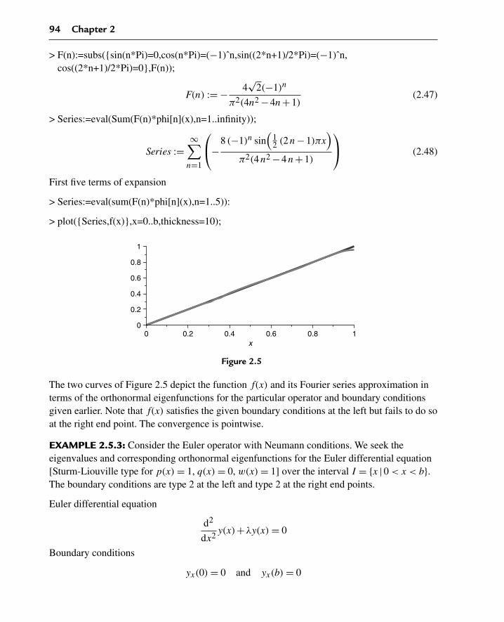
94 Chapter 2
> F(n):=subs({sin(n*Pi)=0,cos(n*Pi)=(−1)ˆn,sin((2*n+1)/2*Pi)=(−1)ˆn,cos((2*n+1)/2*Pi)=0},F(n));
F(n) := − 4√
2(−1)n
π2(4n2 −4n+1)(2.47)
> Series:=eval(Sum(F(n)*phi[n](x),n=1..infinity));
Series :=∞∑
n=1
⎛⎝−
8 (−1)n sin(
12 (2n−1)πx
)π2(4n2 −4n+1)
⎞⎠ (2.48)
First five terms of expansion
> Series:=eval(sum(F(n)*phi[n](x),n=1..5)):
> plot({Series,f(x)},x=0..b,thickness=10);
x0 0.2 0.4 0.6 0.8 1
0
0.2
0.4
0.6
0.8
1
Figure 2.5
The two curves of Figure 2.5 depict the function f(x) and its Fourier series approximation interms of the orthonormal eigenfunctions for the particular operator and boundary conditionsgiven earlier. Note that f(x) satisfies the given boundary conditions at the left but fails to do soat the right end point. The convergence is pointwise.
EXAMPLE 2.5.3: Consider the Euler operator with Neumann conditions. We seek theeigenvalues and corresponding orthonormal eigenfunctions for the Euler differential equation[Sturm-Liouville type for p(x) = 1, q(x) = 0, w(x) = 1] over the interval I = {x |0 < x < b}.The boundary conditions are type 2 at the left and type 2 at the right end points.
Euler differential equation
d2
dx2y(x)+λy(x) = 0
Boundary conditions
yx(0) = 0 and yx(b) = 0
Sturm-Liouville Eigenvalue Problems and Generalized Fourier Series 95
SOLUTION: We consider two possibilities for values of λ. We first consider λ = 0. For thiscase, the system basis vectors are
> restart:y1(x):=1;y2(x):=x;
y1(x) := 1
y2(x) := x (2.49)
General solution
> y(x):=C1*y1(x)+C2*y2(x);
y(x) := C1+C2x (2.50)
Substituting into the boundary conditions yields
> eval(subs(x=0,diff(y(x),x)))=0;
C2 = 0 (2.51)
> eval(subs(x=b,diff(y(x),x)))=0;
C2 = 0 (2.52)
The only nontrivial solution to the above occurs when C2 = 0 and C1 is arbitrary. Thus, oureigenvalue and corresponding eigenfunction for λ = 0 are
> lambda[0]:=0;
λ0 := 0 (2.53)
> phi[0](x):=1;
φ0(x) := 1 (2.54)
We next consider λ > 0. We set λ = μ2. For this case, the system basis vectors are
> y1(x):=sin(mu*x);y2(x):=cos(mu*x);
y1(x) := sin(μx)
y2(x) := cos(μx) (2.55)
General solution
> y(x):=C1*y1(x)+C2*y2(x);
y(x) := C1 sin(μx)+C2 cos(μx) (2.56)

96 Chapter 2
Substituting into the boundary conditions yields
> eval(subs(x=0,diff(y(x),x)))=0;
C1μ = 0 (2.57)
> eval(subs(x=b,diff(y(x),x)))=0;
C1 cos(μb)μ−C2 sin(μb)μ = 0 (2.58)
The only nontrivial solutions to the above occur when C1 = 0, C2 is arbitrary, and μ satisfiesthe following eigenvalue equation:
> sin(mu*b)=0;
sin(μb) = 0 (2.59)
Thus, μ takes on values
> mu[n]:=n*Pi/b;
μn := nπ
b(2.60)
for n = 1,2,3, . . . .
Allowed eigenvalues are λn = μ2n
> lambda[n]:=mu[n]ˆ2;
λn := n2π2
b2(2.61)
Nonnormalized eigenfunctions are
> phi[n](x):=cos(mu[n]*x);
φn(x) := cos(nπx
b
)(2.62)
Normalization
Evaluating the norm from the inner product of the eigenfunctions with respect to the weightfunction w(x) = 1 over the interval, yields, for n = 0
> w(x):=1:norm0:=sqrt(Int(phi[0](x)ˆ2*w(x),x=0..b));
norm0 :=
√√√√√b∫
0
1dx (2.63)

Sturm-Liouville Eigenvalue Problems and Generalized Fourier Series 97
> norm0:=value(%);
norm0 := √b (2.64)
For n = 1,2,3, . . . , we get
> norm1:=sqrt(Int(phi[n](x)ˆ2*w(x),x=0..b));norm1:=expand(value(%)):
norm1 :=
√√√√√b∫
0
cos(nπx
b
)2dx (2.65)
Substitution of the eigenvalue equation simplifies the norm
> norm1:=radsimp(subs({sin(n*Pi)=0,cos(n*Pi)=(−1)ˆn},norm1));
norm1 := 1
2
√2√
b (2.66)
Orthonormal eigenfunctions
> phi[0](x):=phi[0](x)/norm0;
φ0(x) := 1√b
(2.67)
> phi[n](x):=phi[n](x)/norm1;phi[m](x):=subs(n=m,phi[n](x)):
φn(x) := cos(nπxb
)√2√
b(2.68)
Statement of orthonormality
> Int(phi[n](x)*phi[m](x)*w(x),x=0..b)=delta(n,m);
b∫0
2 cos(nπxb
)cos
(mπx
b
)b
dx = δ(n,m) (2.69)
Generalized Fourier series expansion
> f(x):=F(0)*phi[0](x)+Sum(F(n)*phi[n](x),n=1..infinity);f(x):=‘f(x)’:
f(x) := F(0)√b
+∞∑
n=1
F(n) cos(nπxb
)√2√
b(2.70)

98 Chapter 2
Fourier coefficients
> F(n):=Int(f(x)*phi[n](x)*w(x),x=0..b);F(n):=‘F(n)’:
F(n) :=b∫
0
f(x) cos(nπxb
)√2√
bdx (2.71)
> F(0):=Int(f(x)*phi[0](x)*w(x),x=0..b);
F(0) :=b∫
0
f(x)√b
dx (2.72)
This is the generalized series expansion of f(x) in terms of the “complete” set of eigenfunctionsfor the particular Sturm-Liouville operator and boundary conditions over the interval.
DEMONSTRATION: Develop the generalized series expansion for f(x) = x over the intervalI = {x |0 < x < 1} in terms of the preceding eigenfunctions. We assign the system values
> a:=0;b:=1;f(x):=x;
a := 0
b := 1
f(x) := x (2.73)
SOLUTION: We evaluate the Fourier coefficients
> F(n):=eval(Int(f(x)*phi[n](x)*w(x),x=a..b));F(n):=value(%):
F(n) :=1∫
0
x cos(nπx)√
2 dx (2.74)
> F(n):=simplify(subs({sin(n*Pi)=0,cos(n*Pi)=(−1)ˆn},F(n)));
F(n) :=√
2 (−1+ (−1)n)
n2π2(2.75)
> F(0):=eval(Int(f(x)*phi[0](x)*w(x),x=a..b));
F(0) :=1∫
0
xdx (2.76)

Sturm-Liouville Eigenvalue Problems and Generalized Fourier Series 99
> F(0):=value(%);
F(0) := 1
2(2.77)
> Series:=eval(F(0)*phi[0](x)+Sum(F(n)*phi[n](x),n=1..infinity));
Series := 1
2+
∞∑n=1
2(−1+ (−1)n
)cos(nπx)
n2π2(2.78)
First five terms of expansion
> Series:=eval(F(0)*phi[0](x)+sum(F(n)*phi[n](x),n=1..5)):
> plot({Series,f(x)},x=a..b,thickness=10);
x0 0.2 0.4 0.6 0.8 1
0
0.2
0.4
0.6
0.8
1
Figure 2.6
The two curves of Figure 2.6 depict the function f(x) and its Fourier series approximation interms of the orthonormal eigenfunctions for the particular operator and boundary conditionsgiven earlier. Note that f(x) does not satisfy either of the boundary conditions imposed on theeigenfunctions at the end points. The convergence is pointwise.
EXAMPLE 2.5.4: Consider the Euler operator with Dirichlet and Robin conditions. We seekthe eigenvalues and corresponding orthonormal eigenfunctions for the Euler differentialequation [Sturm-Liouville type for p(x) = 1, q(x) = 0, w(x) = 1] over the intervalI = {x |0 < x < b}. The boundary conditions are type 1 at the left and type 3 at the right endpoints.
Euler differential equation
d2
dx2y(x)+λy(x) = 0
Boundary conditions (h > 0)
y(0) = 0 and yx(b)+hy(b) = 0
100 Chapter 2
SOLUTION: We consider two possibilities for values of λ. We first consider λ = 0. For thiscase, the system basis vectors are
> restart:y1(x):=1;y2(x):=x;
y1(x) := 1
y2(x) := x (2.79)
General solution
> y(x):=C1*y1(x)+C2*y2(x);
y(x) := C1+C2x (2.80)
Substituting into the boundary conditions yields
> eval(subs(x=0,y(x)))=0;
C1 = 0 (2.81)
> eval(subs(x=b,diff(y(x),x)+h*y(x)))=0;
C2+h(C1+C2b) = 0 (2.82)
The only solution to the preceding is the trivial solution. We next consider λ > 0. We setλ = μ2, and for this case, the system basis vectors are
> y1(x):=sin(mu*x);y2(x):=cos(mu*x);
y1(x) := sin(μx)
y2(x) := cos(μx) (2.83)
General solution
> y(x):=C1*y1(x)+C2*y2(x);
y(x) := C1 sin(μx)+C2 cos(μx) (2.84)
Substituting into the boundary conditions yields
> eval(subs(x=0,y(x)))=0;
C2 = 0 (2.85)
> eval(subs(x=b,diff(y(x),x)+h*y(x)))=0;
C1 cos(μb)μ−C2 sin(μb)μ+h(C1 sin(μb)+C2 cos(μb)) = 0 (2.86)
Sturm-Liouville Eigenvalue Problems and Generalized Fourier Series 101
The only nontrivial solutions to the preceding are that C2 = 0, C1 is arbitrary, and μ mustsatisfy the following eigenvalue equation:
> h*sin(mu*b)+mu*cos(mu*b)=0;
h sin(μb)+μ cos(μb) = 0 (2.87)
We indicate these roots as μn for n = 1,2,3, . . . .
Allowed eigenvalues are λn = μ2n
> lambda[n]=mu[n]ˆ2;
λn = μ2n (2.88)
Nonnormalized eigenfunctions are
> phi[n](x):=sin(sqrt(lambda[n])*x);
φn(x) := sin(√
λnx)
(2.89)
Normalization
Evaluating the norm from the inner product of the eigenfunctions with respect to the weightfunction w(x) = 1 over the interval yields
> w(x):=1:unprotect(norm):norm:=sqrt(Int(phi[n](x)ˆ2*w(x),x=0..b));norm:=value(%):
norm :=
√√√√√b∫
0
sin(√
λnx)2
dx (2.90)
Substitution of the eigenvalue equation simplifies the norm
> norm:=radsimp(subs(sin(sqrt(lambda[n])*b)=−sqrt(lambda[n])/h*cos(sqrt(lambda[n])*b),norm));
norm := 1
2
√2
√(cos
(√λnb
)2 +bh)
h
h(2.91)
Orthonormal eigenfunctions
> phi[n](x):=phi[n](x)/norm;phi[m](x):=subs(n=m,phi[n](x)):
φn(x) := sin(√
λnx)√
2h√(cos
(√λnb
)2 +bh)
h
(2.92)

102 Chapter 2
Statement of orthonormality
> Int(phi[n](x)*phi[m](x)*w(x),x=0..b)=delta(n,m);
b∫0
2 sin(√
λnx)h2 sin
(√λmx
)√(
cos(√
λnb)2 +bh
)h
√(cos
(√λmb
)2 +bh)
h
dx = δ(n,m) (2.93)
Generalized Fourier series expansion
> f(x):=Sum(F(n)*phi[n](x),n=1..infinity);f(x):=‘f(x)’:
f(x) :=∞∑
n=1
F(n) sin(√
λn x) √
2h√(cos
(√λnb
)2 +bh)
h
(2.94)
Fourier coefficients
> F(n):=Int(f(x)*phi[n](x)*w(x),x=0..b);F(n):=‘F(n)’:
F(n) :=b∫
0
f(x) sin(√
λn x) √
2h√(cos
(√λnb
)2 +bh)
h
dx (2.95)
This is the generalized series expansion of f(x) in terms of the “complete” set of eigenfunctionsfor the particular Sturm-Liouville operator and boundary conditions over the interval.
DEMONSTRATION: Develop the generalized series expansion for f(x) = x over the intervalI = {x |0 < x < 1} in terms of the preceding eigenfunctions for h = 1. We assign the systemvalues
> a:=0;b:=1;h:=1;f(x):=x;
a := 0
b := 1
h := 1
f(x) := x (2.96)
SOLUTION: We evaluate the Fourier coefficients
> F(n):=Int(eval(f(x)*phi[n](x))*w(x),x=a..b);F(n):=value(%):
F(n) :=1∫
0
x sin(√
λn x) √
2√cos
(√λn
)2 +1dx (2.97)

Sturm-Liouville Eigenvalue Problems and Generalized Fourier Series 103
Substitution of the eigenvalue equation simplifies the preceding equation:
> F(n):=simplify(subs(sin(sqrt(lambda[n])*b)=−sqrt(lambda[n])/h*cos(sqrt(lambda[n])*b),F(n)));
F(n) := − 2√
2 cos(√
λn
)√
cos(√
λn
)2 +1√
λn
(2.98)
> Series:=simplify(Sum(F(n)*phi[n](x),n=1..infinity));
Series :=∞∑
n=1
⎛⎝−4 cos
(√λn
)sin
(√λnx
)(
cos(√
λn
)2 +1)√
λn
⎞⎠ (2.99)
Evaluation of the eigenvalues from the roots of the eigenvalue equation yields
> tan(sqrt(lambda[n])*b)=−sqrt(lambda[n])/h;
tan(√
λn
)= −√
λn (2.100)
> plot({tan(v),−v/(b*h)},v=0..20,y=−20..0,thickness=10);
v10 20
y
220
215
210
25
0155
Figure 2.7
If we set v = √λb, then the eigenvalues are found from the intersection points of the curves
shown in Figure 2.7. We evaluate a few of these eigenvalues from the Maple fsolve commandfor the roots of the eigenvalue equation to be given as
> lambda[1]:=(1/b*(fsolve((tan(v)+v/(h*b)),v=1..3)))ˆ2;
λ1 := 4.115858365 (2.101)
> lambda[2]:=(1/b*(fsolve((tan(v)+v/(h*b)),v=3..6)))ˆ2;
λ2 := 24.13934203 (2.102)

104 Chapter 2
> lambda[3]:=(1/b*(fsolve((tan(v)+v/(h*b)),v=6..9)))ˆ2;
λ3 := 63.65910654 (2.103)
> lambda[4]:=(1/b*(fsolve((tan(v)+v/(h*b)),v=9..13)))ˆ2;
λ4 := 122.8891618 (2.104)
> lambda[5]:=(1/b*(fsolve((tan(v)+v/(h*b)),v=13..16)))ˆ2;
λ5 := 201.8512584 (2.105)
First five terms of expansion
> Series:=eval(sum(F(n)*phi[n](x),n=1..5)):
> plot({Series,f(x)},x=a..b,thickness=10);
x0 0.2 0.4 0.6 0.8 1
0
0.2
0.4
0.6
0.8
1
Figure 2.8
The two curves of Figure 2.8 depict the function f(x) and its Fourier series approximation interms of the orthonormal eigenfunctions for the particular operator and boundary conditionsgiven earlier. Note that f(x) satisfies the given boundary conditions at the left but fails to do soat the right end point. The convergence is pointwise.
EXAMPLE 2.5.5: Consider the Euler operator with Neumann and Robin conditions. We seekthe eigenvalues and corresponding orthonormal eigenfunctions for the Euler differentialequation [Sturm-Liouville type for p(x) = 1, q(x) = 0, w(x) = 1] over the intervalI = {x |0 < x < b}. The boundary conditions are type 2 at the left and type 3 at the right endpoints.
Euler differential equation
d2
dx2y(x)+λy(x) = 0

Sturm-Liouville Eigenvalue Problems and Generalized Fourier Series 105
Boundary conditions (h > 0)
yx(0) = 0 and yx(b)+hy(b) = 0
SOLUTION: We consider two possibilities for values of λ. We first consider λ = 0. For thiscase, the system basis vectors are
> restart:y1(x):=1;y2(x):=x;
y1(x) := 1
y2(x) := x (2.106)
General solution
> y(x):=C1*y1(x)+C2*y2(x);
y(x) := C1+C2x (2.107)
Substituting into the boundary conditions yields
> eval(subs(x=0,diff(y(x),x)))=0;
C2 = 0 (2.108)
> eval(subs(x=b,diff(y(x),x)+h*y(x)))=0;
C2+h(C1+C2b) = 0 (2.109)
The only solution to the preceding is the trivial solution. We next consider λ > 0. We setλ = μ2. For this case, the system basis vectors are
> y1(x):=sin(mu*x); y2(x):=cos(mu*x);
y1(x) := sin(μx)
y2(x) := cos(μx) (2.110)
General solution
> y(x):=C1*y1(x)+C2*y2(x);
y(x) := C1 sin(μx)+C2 cos(μx) (2.111)
Substituting into the boundary conditions yields
> eval(subs(x=0,diff(y(x),x)))=0;
C1μ = 0 (2.112)

106 Chapter 2
> eval(subs(x=b,diff(y(x),x)+h*y(x)))=0;
C1 cos(μb)μ−C2 sin(μb)μ+h(C1 sin(μb)+C2 cos(μb)) = 0 (2.113)
The only nontrivial solutions to the preceding occur when C1 = 0, C2 is arbitrary, and μ
satisfies the following eigenvalue equation:
> mu*sin(mu*b)−h*cos(mu*b)=0;
μ sin(μb)−h cos(μb) = 0 (2.114)
We identify these roots as μn for n = 1,2,3, . . . .
Allowed eigenvalues are λn = μ2n
> lambda[n]=mu[n]ˆ2;
λn = μ2n (2.115)
Nonnormalized eigenfunctions are
> phi[n](x):=cos(sqrt(lambda[n])*x);
φn(x) := cos(√
λnx)
(2.116)
Normalization
Evaluating the norm from the inner product of the eigenfunctions with respect to the weightfunction w(x) = 1 over the interval yields
> w(x):=1:unprotect(norm):norm:=sqrt(Int(phi[n](x)ˆ2*w(x),x=0..b));norm:=value(%):
norm :=
√√√√√b∫
0
cos(√
λnx)2
dx (2.117)
Substitution of the eigenvalue equation simplifies the preceding equation:
> norm:=radsimp(subs(cos(sqrt(lambda[n])*b)=sqrt(lambda[n])/h*sin(sqrt(lambda[n])*b),norm));
norm := 1
2
√2
√(sin
(√λnb
)2 +bh)
h
h(2.118)

Sturm-Liouville Eigenvalue Problems and Generalized Fourier Series 107
Orthonormal eigenfunctions
> phi[n](x):=phi[n](x)/norm;phi[m](x):=subs(n=m,phi[n](x)):
φn(x) := cos(√
λnx)√
2h√(sin
(√λnb
)2 +bh)
h
(2.119)
Statement of orthonormality
> Int(phi[n](x)*phi[m](x)*w(x),x=0..b)=delta(n,m);;
b∫0
2 cos(√
λnx)h2 cos
(√λmx
)√(
sin(√
λnb)2 +bh
)h
√(sin
(√λmb
)2 +bh)
h
dx = δ(n,m) (2.120)
Generalized Fourier series expansion
> f(x):=Sum(F(n)*phi[n](x),n=1..infinity);f(x):=‘f(x)’:
f(x) :=∞∑
n=1
F(n) cos(√
λnx)√
2h√(sin
(√λnb
)2 +bh)
h
(2.121)
Fourier coefficients
> F(n):=Int(f(x)*phi[n](x)*w(x),x=0..b);F(n):=‘F(n)’:
F(n) :=b∫
0
f(x) cos(√
λnx)√
2h√(sin
(√λnb
)2 +bh)
h
dx (2.122)
This is the generalized series expansion of f(x) in terms of the “complete” set of eigenfunctionsfor the particular Sturm-Liouville operator and boundary conditions over the interval.
DEMONSTRATION: Develop the generalized series expansion for f(x) = 1−x over theinterval I = {x |0 < x < 1} in terms of the preceding eigenfunctions for h = 1. We assign thesystem values
> a:=0;b:=1;h:=1;f(x):=1−x;
a := 0
b := 1
h := 1
f(x) := 1−x (2.123)

108 Chapter 2
SOLUTION: We evaluate the Fourier coefficients
> F(n):=Int(eval(f(x)*phi[n](x))*w(x),x=a..b);F(n):=value(%):
F(n) :=1∫
0
(1−x) cos(√
λnx)√
2√sin
(√λn
)2 +1dx (2.124)
> F(n):=radsimp(subs(tan(sqrt(lambda[n])*b)=h/sqrt(lambda[n]),F(n)));
F(n) :=(1− cos
(√λn
))√2
λn
√2− cos
(√λn
)2(2.125)
> Series:=simplify(Sum(F(n)*phi[n](x),n=1..infinity));
Series :=∞∑
n=1
2(−1+ cos
(√λn
))cos
(√λnx
)λn
(−2+ cos
(√λn
)2) (2.126)
Evaluation of the eigenvalues from the roots of the eigenvalue equation yields
> tan(sqrt(lambda[n])*b)=h/sqrt(lambda[n]);
tan(√
λn
)= 1√
λn(2.127)
> plot({tan(v),(h*b)/v},v=0..20,y=0..3/2,thickness=10);
v0 5 10 15 20
y
0
0.5
1.0
1.5
Figure 2.9
If we set v = √λb, then the eigenvalues are found from the intersection points of the curves
shown in Figure 2.9. We evaluate a few of these eigenvalues from the Maple fsolve commandfor the roots of the eigenvalue equation to be given as

Sturm-Liouville Eigenvalue Problems and Generalized Fourier Series 109
> lambda[1]:=(1/b*(fsolve((tan(v)−(h*b)/v),v=0..1)))ˆ2;
λ1 := 0.7401738844 (2.128)
> lambda[2]:=(1/b*(fsolve((tan(v)−(h*b)/v),v=1..4)))ˆ2;
λ2 := 11.73486183 (2.129)
> lambda[3]:=(1/b*(fsolve((tan(v)−(h*b)/v),v=4..7)))ˆ2;
λ3 := 41.43880785 (2.130)
> lambda[4]:=(1/b*(fsolve((tan(v)−(h*b)/v),v=7..10)))ˆ2;
λ4 := 90.80821420 (2.131)
> lambda[5]:=(1/b*(fsolve((tan(v)−(h*b)/v),v=10..13)))ˆ2;
λ5 := 159.9032889 (2.132)
First five terms of expansion
> Series:=eval(sum(F(n)*phi[n](x),n=1..5)):
> plot({Series,f(x)},x=a..b,thickness=10);
x0 0.2 0.4 0.6 0.8 1
0
0.2
0.4
0.6
0.8
1
Figure 2.10
The two curves of Figure 2.10 depict the function f(x) and its Fourier series approximation interms of the orthonormal eigenfunctions for the particular operator and boundary conditionsgiven earlier. Note that f(x) does not satisfy either of the given boundary conditions at the leftor right end points. The convergence is pointwise.
EXAMPLE 2.5.6: Consider the Euler operator with Robin and Dirichlet conditions. We seekthe eigenvalues and corresponding orthonormal eigenfunctions for the Euler differentialequation [Sturm-Liouville type for p(x) = 1, q(x) = 0,w(x) = 1] over the interval

110 Chapter 2
I = {x |0 < x < b}. The boundary conditions are type 3 at the left and type 1 at the right endpoints.
Euler differential equation
d2
dx2y(x)+λy(x) = 0
Boundary conditions (h > 0)
yx(0)−hy(0) = 0 and y(b) = 0
SOLUTION: We consider two possibilities for values of λ. We first consider λ = 0. For thiscase, the system basis vectors are
> restart:y1(x):=1;y2(x):=x;
y1(x) := 1(2.133)
y2(x) := x
General solution
> y(x):=C1*y1(x)+C2*y2(x);
y(x) := C1+C2x (2.134)
Substituting into the boundary conditions yields
> eval(subs(x=0,diff(y(x),x)−h*y(x)))=0;
C2−hC1 = 0 (2.135)
> eval(subs(x=b,y(x)))=0;
C1+C2b = 0 (2.136)
The only solution to the above is the trivial solution. We next consider λ > 0. We set λ = μ2,and, for this case, the system basis vectors are
> y1(x):=sin(mu*x);y2(x):=cos(mu*x);
y1(x) := sin(μx)(2.137)
y2(x) := cos(μx)
General solution
Sturm-Liouville Eigenvalue Problems and Generalized Fourier Series 111
> y(x):=C1*y1(x)+C2*y2(x);
y(x) := C1 sin(μx)+C2 cos(μx) (2.138)
Substituting into the boundary conditions yields
> eval(subs(x=0,diff(y(x),x)−h*y(x)))=0;
C1μ−hC2 = 0 (2.139)
> eval(subs(x=b,y(x)))=0;
C1 sin(μb)+C2 cos(μb) = 0 (2.140)
The only nontrivial solutions to the preceding occur when both C1 and C2 are arbitrary and μ
satisfies the following eigenvalue equation:
> h*sin(mu*b)+mu*cos(mu*b)=0;
h sin(μb)+μ cos(μb) = 0 (2.141)
We identify these roots as μn for n = 1,2,3, . . . .
Allowed eigenvalues are λn = μ2n
> lambda[n]=mu[n]ˆ2;
λn = μ2n (2.142)
Nonnormalized eigenfunctions are
> phi[n](x):=h*sin(sqrt(lambda[n])*x)+sqrt(lambda[n])*cos(sqrt(lambda[n])*x);
φn(x) := h sin(√
λnx)
+√λn cos
(√λnx
)(2.143)
Normalization
Evaluating the norm from the inner product of the eigenfunctions with respect to the weightfunction w(x) = 1 over the interval yields
> w(x):=1:unprotect(norm):norm:=sqrt(Int(phi[n](x)ˆ2*w(x),x=0..b));norm:=value(%):
norm :=
√√√√√b∫
0
(h sin
(√λnx
)+√
λn cos(√
λnx))2
dx (2.144)

112 Chapter 2
Substitution of the eigenvalue equation simplifies the preceding equation:
> norm:=radsimp(subs(sin(sqrt(lambda[n])*b)=−sqrt(lambda[n])/h*cos(sqrt(lambda[n])*b),norm));
norm := 1
2
√2
√−
(−2h2 +h2 cos
(√λnb
)2 −h3b+λn cos(√
λnb)2 −λnbh
)h
h(2.145)
Orthonormal eigenfunctions
> phi[n](x):=phi[n](x)/norm;phi[m](x):=subs(n=m,phi[n](x)):
φn(x) :=(h sin
(√λnx
)+√λn cos
(√λnx
))√2h√
−(−2h2 +h2 cos
(√λnb
)2 −h3b+λn cos(√
λnb)2 −λnbh
)h
(2.146)
Statement of orthonormality
> Int(phi[n](x)*phi[m](x)*w(x),x=0..b)=delta(n,m);;
b∫0
(2(h sin
(√λnx
)+√
λn cos(√
λnx))
h2(h sin
(√λmx
)+√
λm cos(√
λmx)))/
(√−
(−2h2 +h2 cos
(√λnb
)2 −h3b+λn cos(√
λnb)2 −λnbh
)h
√−
(−2h2 +h2 cos
(√λmb
)2 −h3b+λm cos(√
λmb)2 −λmbh
)h
)dx = δ(n,m)
(2.147)
Generalized Fourier series expansion
> f(x):=Sum(F(n)*phi[n](x),n=1..infinity);f(x):=‘f(x)’:
f(x) :=∞∑
n=1
F(n)(h sin
(√λnx
)+√λn cos
(√λnx
))√2h√
−(−2h2 +h2 cos
(√λnb
)2 −h3b+λn cos(√
λnb)2 −λnbh
)h
(2.148)

Sturm-Liouville Eigenvalue Problems and Generalized Fourier Series 113
Fourier coefficients
> F(n):=Int(f(x)*phi[n](x)*w(x),x=0..b);F(n):=‘F(n)’:
F(n) :=b∫
0
f(x)(h sin
(√λnx
)+√λn cos
(√λnx
))√2h√
−(−2h2 +h2 cos
(√λnb
)2 −h3b+λn cos(√
λnb)2 −λnbh
)h
dx (2.149)
This is the generalized series expansion of f(x) in terms of the “complete” set of eigenfunctionsfor the particular Sturm-Liouville operator and boundary conditions over the interval.
DEMONSTRATION: Develop the generalized series expansion for f(x) = 1−x over theinterval I = {x |0 < x < 1} in terms of the preceding eigenfunctions for h = 1. We assign thesystem values
> a:=0;b:=1;h:=1;f(x):=1−x;
a := 0
b := 1
h := 1
f(x) := 1−x (2.150)
SOLUTION: We evaluate the Fourier coefficients
> F(n):=Int(eval(f(x)*phi[n](x))*w(x),x=a..b);F(n):=value(%):
F(n) :=1∫
0
(1−x)(sin
(√λnx
)+√λn cos
(√λnx
))√2√
3− cos(√
λn
)2 −λn cos(√
λn
)2 +λn
dx (2.151)
> F(n):=radsimp(subs(sin(sqrt(lambda[n])*b)=−sqrt(lambda[n])/h*cos(sqrt(lambda[n])*b),F(n)));
F(n) := 2√
2√
λn
√3− cos
(√λn
)2 −λn cos(√
λn
)2 +λn
(2.152)
> Series:=simplify(Sum(F(n)*phi[n](x),n=1..infinity));
Series :=∞∑
n=1
⎛⎝− 4
(sin
(√λnx
)+√λn cos
(√λnx
))√
λn
(−3+ cos
(√λn
)2 +λn cos(√
λn
)2 −λn
)⎞⎠ (2.153)

114 Chapter 2
Evaluation of the eigenvalues from the roots of the eigenvalue equation yields
> tan(sqrt(lambda[n])*b)=−sqrt(lambda[n])/h;
tan(√
λn
)= −√
λn (2.154)
> plot({tan(v),−v/(h*b)},v=0..20,y=−20..0,thickness=10);
v5 10 15 20
y
220
215
210
25
0
Figure 2.11
If we set v = √λb, then the eigenvalues are found from the intersection points of the curves
shown in Figure 2.11. We evaluate a few of these eigenvalues from the Maple fsolve commandfor the roots of the eigenvalue equation to be given as
> lambda[1]:=(1/b*(fsolve((tan(v)+v/(b*h)),v=1..3)))ˆ2;
λ1 := 4.115858365 (2.155)
> lambda[2]:=(1/b*(fsolve((tan(v)+v/(b*h)),v=3..6)))ˆ2;
λ2 := 24.13934203 (2.156)
> lambda[3]:=(1/b*(fsolve((tan(v)+v/(b*h)),v=6..9)))ˆ2;
λ3 := 63.65910654 (2.157)
> lambda[4]:=(1/b*(fsolve((tan(v)+v/(b*h)),v=10..12)))ˆ2;
λ4 := 122.8891618 (2.158)
> lambda[5]:=(1/b*(fsolve((tan(v)+v/(b*h)),v=13..15)))ˆ2;
λ5 := 201.8512584 (2.159)
First five terms of expansion
> Series:=eval(sum(F(n)*phi[n](x),n=1..5)):> plot({Series,f(x)},x=a..b,thickness=10);
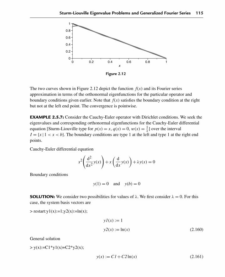
Sturm-Liouville Eigenvalue Problems and Generalized Fourier Series 115
x0 0.2 0.4 0.6 0.8 1
0
0.2
0.4
0.6
0.8
1
Figure 2.12
The two curves shown in Figure 2.12 depict the function f(x) and its Fourier seriesapproximation in terms of the orthonormal eigenfunctions for the particular operator andboundary conditions given earlier. Note that f(x) satisfies the boundary condition at the rightbut not at the left end point. The convergence is pointwise.
EXAMPLE 2.5.7: Consider the Cauchy-Euler operator with Dirichlet conditions. We seek theeigenvalues and corresponding orthonormal eigenfunctions for the Cauchy-Euler differentialequation [Sturm-Liouville type for p(x) = x, q(x) = 0, w(x) = 1
x ] over the intervalI = {x |1 < x < b}. The boundary conditions are type 1 at the left and type 1 at the right endpoints.
Cauchy-Euler differential equation
x2
(d2
dx2y(x)
)+x
(d
dxy(x)
)+λy(x) = 0
Boundary conditions
y(1) = 0 and y(b) = 0
SOLUTION: We consider two possibilities for values of λ. We first consider λ = 0. For thiscase, the system basis vectors are
> restart:y1(x):=1;y2(x):=ln(x);
y1(x) := 1
y2(x) := ln(x) (2.160)
General solution
> y(x):=C1*y1(x)+C2*y2(x);
y(x) := C1+C2 ln(x) (2.161)

116 Chapter 2
Substituting into the boundary conditions yields
> eval(subs(x=1,y(x)))=0;
C1 = 0 (2.162)
> eval(subs(x=b,y(x)))=0;
C1+C2 ln(b) = 0 (2.163)
The only solution to the preceding is the trivial solution. We next consider λ > 0. We setλ = μ2, and, for this case, the system basis vectors are
> y1(x):=sin(mu*ln(x));y2(x):=cos(mu*ln(x));
y1(x) := sin(μ ln(x))
y2(x) := cos(μ ln(x)) (2.164)
General solution
> y(x):=C1*y1(x)+C2*y2(x);
y(x) := C1 sin(μ ln(x))+C2 cos(μ ln(x)) (2.165)
Substituting into the boundary conditions yields
> eval(subs(x=1,y(x)))=0;
C2 = 0 (2.166)
> eval(subs(x=b,y(x)))=0;
C1 sin(μ ln(b))+C2 cos(μ ln(b)) = 0 (2.167)
The only nontrivial solutions to the preceding occur when C2 = 0, C1 is arbitrary, and μ
satisfies the following eigenvalue equation:
> sin(mu*ln(b))=0;
sin(μ ln(b)) = 0 (2.168)
Thus, the values for μ are
> mu[n]:=n*Pi/ln(b);
μn := nπ
ln(b)(2.169)
for n = 1,2,3, . . . .
Sturm-Liouville Eigenvalue Problems and Generalized Fourier Series 117
Allowed eigenvalues are λn = μ2n
> lambda[n]:=(n*Pi/ln(b))ˆ2;
λn := n2π2
ln(b)2(2.170)
Nonnormalized eigenfunctions are
> phi[n](x):=(sin(mu[n]*ln(x)));
φn(x) := sin
(nπ ln(x)
ln(b)
)(2.171)
Normalization
Evaluating the norm from the inner product of the eigenfunctions with respect to the weightfunction w(x) = 1
x over the interval yields
> w(x):=1/x:unprotect(norm):norm:=sqrt(Int(phi[n](x)ˆ2*w(x),x=1..b));norm:=value(%):
norm :=
√√√√√√b∫
1
sin(
nπ ln(x)ln(b)
)2
xdx (2.172)
Substitution of the eigenvalue equation simplifies the norm
> norm:=radsimp(subs({sin(n*Pi)=0,cos(n*Pi)=(−1)ˆn},norm));
norm := 1
2
√2√
ln(b) (2.173)
Orthonormal eigenfunctions
> phi[n](x):=phi[n](x)/norm;phi[m](x):=subs(n=m,phi[n](x)):
φn(x) :=sin
(nπ ln(x)
ln(b)
)√2
√ln(b)
(2.174)
Statement of orthonormality
> Int(phi[n](x)*phi[m](x)*w(x),x=1..b)=delta(n,m);;
b∫1
2 sin(
nπ ln(x)ln(b)
)sin
(mπ ln(x)
ln(b)
)ln(b)x
dx = δ(n,m) (2.175)

118 Chapter 2
Generalized Fourier series expansion
> f(x):=Sum(F(n)*phi[n](x),n=1..infinity);f(x):=‘f(x)’:
f(x) :=∞∑
n=1
F(n) sin(
nπ ln(x)ln(b)
)√2
√ln(b)
(2.176)
Fourier coefficients
> F(n):=Int(f(x)*phi[n](x)*w(x),x=1..b);F(n):=‘F(n)’:
F(n) :=b∫
1
f(x) sin(
nπ ln(x)ln(b)
)√2
√ln(b)x
dx (2.177)
This is the generalized series expansion of f(x) in terms of the “complete” set of eigenfunctionsfor the particular Sturm-Liouville operator and boundary conditions over the interval.
DEMONSTRATION: Develop the generalized series expansion for f(x) = x−1 over theinterval I = {x |1 < x < 2} in terms of the preceding eigenfunctions. We assign the systemvalues
> a:=1;b:=2;f(x):=x−1;
a : = 1
b : = 2
f(x) : = x−1 (2.178)
SOLUTION: We evaluate the Fourier coefficients
> F(n):=eval(Int(f(x)*phi[n](x)*w(x),x=a..b));F(n):=simplify(value(%)):
F(n) :=2∫
1
(x−1) sin(
nπ ln(x)ln(2)
)√2
√ln(2)x
dx (2.179)
> F(n):=combine(%,trig):F(n):=subs(cos(n*Pi)=(−1)ˆn,sin(n*Pi)=0,F(n));
F(n) := −√ln(2)
√2n2π2(−1)n − ln(2)5/2
√2+ ln(2)5/2
√2(−1)n
n3π3 +nπ ln(2)2(2.180)

Sturm-Liouville Eigenvalue Problems and Generalized Fourier Series 119
> Series:=eval(Sum(F(n)*phi[n](x),n=1..infinity));
Series :=∞∑
n=1
(−√
ln(2)√
2n2π2(−1)n − ln(2)5/2√
2+ ln(2)5/2√
2(−1)n)
sin(
nπ ln(x)ln(2)
)√2(
n3π3 +nπ ln(2)2)√
ln(2)
(2.181)
First few terms of expansion
> Series:=eval(sum(F(n)*phi[n](x),n=1..5)):
> plot({Series,f(x)},x=a..b,thickness=10);
x1.21 1.4 1.6 1.8 2
0.0
0.2
0.4
0.6
0.8
1
Figure 2.13
The two curves in Figure 2.13 depict the function f(x) and its Fourier series approximation interms of the orthonormal eigenfunctions for the particular operator and boundary conditionsgiven earlier. Note that f(x) satisfies the given boundary conditions at the left but fails to do soat the right end point. The convergence is pointwise.
EXAMPLE 2.5.8: Consider the Cauchy-Euler operator with Neumann and Dirichletconditions. We seek the eigenvalues and corresponding orthonormal eigenfunctions for theCauchy-Euler differential equation [Sturm-Liouville type for p(x) = x, q(x) = 0, w(x) = 1
x ]over the interval I = {x |1 < x < b}. The boundary conditions are type 2 at the left and type 1at the right end points.
Cauchy-Euler differential equation
x2
(d2
dx2y(x)
)+x
(d
dxy(x)
)+λy(x) = 0
Boundary conditions
yx(1) = 0 and y(b) = 0

120 Chapter 2
SOLUTION: We consider two possibilities for values of λ. We first consider λ = 0. For thiscase, the system basis vectors are
> restart:y1(x):=1;y2(x):=ln(x);
y1(x) := 1
y2(x) := ln(x) (2.182)
General solution
> y(x):=C1*y1(x)+C2*y2(x);
y(x) := C1+C2 ln(x) (2.183)
Substituting into the boundary conditions yields
> eval(subs(x=1,diff(y(x),x)))=0;
C2 = 0 (2.184)
> eval(subs(x=b,y(x)))=0;
C1+C2 ln(b) = 0 (2.185)
The only solution to the preceding is the trivial solution. We next consider λ > 0. We setλ = μ2, and, for this case, the system basis vectors are
> y1(x):=sin(mu*ln(x));y2(x):=cos(mu*ln(x));
y1(x) := sin(μ ln(x))
y2(x) := cos(μ ln(x)) (2.186)
General solution
> y(x):=C1*y1(x)+C2*y2(x);
y(x) := C1 sin(μ ln(x))+C2 cos(μ ln(x)) (2.187)
Substituting into the boundary conditions yields
> eval(subs(x=1,diff(y(x),x)))=0;
C1μ = 0 (2.188)
> eval(subs(x=b,y(x)))=0;
C1 sin(μ ln(b))+C2 cos(μ ln(b)) = 0 (2.189)

Sturm-Liouville Eigenvalue Problems and Generalized Fourier Series 121
The only nontrivial solutions to the preceding occur when C1 = 0, C2 is arbitrary, and μ
satisfies the following eigenvalue equation:
> cos(mu*ln(b))=0;
cos(μ ln(b)) = 0 (2.190)
Thus, μ takes on the values
> mu[n]:=(2*n−1)*Pi/(2*ln(b));
μn := 1
2
(2n−1)π
ln(b)(2.191)
for n = 1,2,3, . . . .
Allowed eigenvalues are λn = μ2n
> lambda[n]:=mu[n]ˆ2;
λn := 1
4
(2n−1)2π2
ln(b)2(2.192)
Nonnormalized eigenfunctions are
> phi[n](x):=cos(mu[n]*ln(x));
φn(x) := cos
(1
2
(2n−1)π ln(x)
ln(b)
)(2.193)
Normalization
Evaluating the norm from the inner product of the eigenfunctions with respect to the weightfunction w(x) = 1
x over the interval yields
> w(x):=1/x:unprotect(norm):norm:=sqrt(Int(phi[n](x)ˆ2*w(x),x=1..b));norm:=expand(value(%)):
norm :=
√√√√√√b∫
1
cos(
12
(2n−1)π ln(x)ln(b)
)2
xdx (2.194)
Substitution of the eigenvalue equation simplifies the norm
> norm:=radsimp(subs({sin(n*Pi)=0,cos(n*Pi)=(−1)ˆn},norm));
norm := 1
2
√2√
ln(b) (2.195)

122 Chapter 2
Orthonormal eigenfunctions
> phi[n](x):=phi[n](x)/norm;phi[m](x):=subs(n=m,phi[n](x)):
φn(x) :=cos
(12
(2n−1)π ln(x)ln(b)
)√2
√ln(b)
(2.196)
Statement of orthonormality
> Int(phi[n](x)*phi[m](x)*w(x),x=1..b)=delta(n,m);
b∫1
2 cos(
12
(2n−1)π ln(x)ln(b)
)cos
(12
(2m−1)π ln(x)ln(b)
)ln(b)x
dx = δ(n,m) (2.197)
Generalized Fourier series expansion
> f(x):=Sum(F(n)*phi[n](x),n=1..infinity);f(x):=‘f(x)’:
f(x) :=∞∑
n=1
F(n) cos(
12
(2n−1)π ln(x)ln(b)
)√2
√ln(b)
(2.198)
Fourier coefficients
> F(n):=Int(f(x)*phi[n](x)*w(x),x=1..b);F(n):=‘F(n)’:
F(n) :=b∫
1
f(x) cos(
12
(2n−1)π ln(x)ln(b)
)√2
√ln(b)x
dx (2.199)
This is the generalized series expansion of f(x) in terms of the “complete” set ofeigenfunctions for the particular Sturm-Liouville operator and boundary conditions over theinterval.
DEMONSTRATION: Develop the generalized series expansion for f(x) = 2x−x2 over theinterval I = {x |1 < x < 2} in terms of the preceding eigenfunctions. We assign the systemvalues
> a:=1;b:=2;f(x):=2*x−xˆ2;
a := 1
b := 2
f(x) := 2x−x2 (2.200)

Sturm-Liouville Eigenvalue Problems and Generalized Fourier Series 123
SOLUTION: We evaluate the Fourier coefficients
> F(n):=eval(Int(f(x)*phi[n](x)*w(x),x=a..b));F(n):=simplify(value(%)):
F(n) :=2∫
1
(2x−x2) cos(
12
(2n−1)π ln(x)ln(2)
)√2
√ln(2) x
dx (2.201)
> F(n):=combine(%,trig):F(n):=factor(simplify(subs(cos(n*Pi)=(−1)ˆn,sin(n*Pi)=0,F(n))));
F(n) := − 96 ln(2)5/2√
2(2πn(−1)n −π(−1)n + ln(2)
)(16 ln(2)2 −4π2n+π2 +4π2n2
) (4π2n2 −4π2n+4 ln(2)2 +π2
) (2.202)
> Series:=eval(Sum(F(n)*phi[n](x),n=1..infinity));
Series :=∞∑
n=1
⎛⎝−
192 ln(2)2 (2πn(−1)n −π(−1)n + ln(2)
)cos
(12
(2n−1)π ln(x)ln(2)
)(16 ln(2)2 −4π2n+π2 +4π2n2
) (4π2n2 −4π2n+4 ln(2)2 +π2
)⎞⎠
(2.203)
First five terms of expansion
> Series:=eval(sum(F(n)*phi[n](x),n=1..5)):
> plot({Series,f(x)},x=a..b,thickness=10);
x1.21 1.4 1.6 1.8 2
0
0.2
0.4
0.6
0.8
1
Figure 2.14
The two curves in Figure 2.14 depict the function f(x) and its Fourier series approximation interms of the orthonormal eigenfunctions for the particular operator and boundary conditionsgiven earlier. Note that f(x) satisfies the given boundary conditions at both the left and theright end points. The convergence is uniform.
124 Chapter 2
EXAMPLE 2.5.9: Consider the Cauchy-Euler operator with Dirichlet and Robin conditions.We seek the eigenvalues and corresponding orthonormal eigenfunctions for the Cauchy-Eulerdifferential equation [Sturm-Liouville type for p(x) = x, q(x) = 0, w(x) = 1
x ] over the intervalI = {x |1 < x < b}. The boundary conditions are type 3 at the left and type 1 at the right endpoints.
Cauchy-Euler differential equation
x2
(d2
dx2y(x)
)+x
(d
dxy(x)
)+λy(x) = 0
Boundary conditions (h > 0)
y(1) = 0 and yx(b)+hy(b) = 0
SOLUTION: We consider two possibilities for values of λ. We first consider λ = 0. For thiscase, the system basis vectors are
> restart:y1(x):=1;y2(x):=ln(x);
y1(x) := 1
y2(x) := ln(x) (2.204)
General solution
> y(x):=C1*y1(x)+C2*y2(x);
y(x) := C1+C2 ln(x) (2.205)
Substituting into the boundary conditions yields
> eval(subs(x=1,y(x)))=0;
C1 = 0 (2.206)
> eval(subs(C1=0,x=b,diff(y(x),x)+h*y(x)))=0;
C2
b+hC2 ln(b) = 0 (2.207)
The only solution to the preceding is the trivial solution. We next consider λ > 0. We setλ = μ2, and, for this case, the system basis vectors are
> y1(x):=sin(mu*ln(x));y2(x):=cos(mu*ln(x));
y1(x) := sin(μ ln(x))
y2(x) := cos(μ ln(x)) (2.208)

Sturm-Liouville Eigenvalue Problems and Generalized Fourier Series 125
General solution
> y(x):=C1*y1(x)+C2*y2(x);
y(x) := C1 sin(μ ln(x))+C2 cos(μ ln(x)) (2.209)
Substituting into the boundary conditions yields
> eval(subs(x=1,y(x)))=0;
C2 = 0 (2.210)
> eval(subs(C2=0,x=b,diff(y(x),x)+h*y(x)))=0;
C1 cos(μ ln(b))μ
b+hC1 sin(μ ln(b)) = 0 (2.211)
The only nontrivial solutions to the preceding are that C2 = 0, C1 is arbitrary, and μ mustsatisfy the following eigenvalue equation:
> h*sin(mu*ln(b))+mu/b*cos(mu*ln(b))=0;
h sin(μ ln(b))+ μ cos(μ ln(b))
b= 0 (2.212)
We indicate these roots as μn for n = 1,2,3, . . . .
Allowed eigenvalues are λn = μ2n
> lambda[n]=mu[n]ˆ2;
λn = μ2n (2.213)
Nonnormalized eigenfunctions are
> phi[n](x):=sin(sqrt(lambda[n])*ln(x));
φn(x) := sin(√
λn ln(x))
(2.214)
Normalization
Evaluating the norm from the inner product of the eigenfunctions with respect to the weightfunction w(x) = 1
x over the interval yields
> w(x):=1/x:unprotect(norm):norm:=sqrt(Int(phi[n](x)ˆ2*w(x),x=1..b));norm:=value(%):
norm :=
√√√√√b∫
1
sin(√
λn ln(x))2
xdx (2.215)

126 Chapter 2
Substitution of the eigenvalue equation simplifies the norm
> norm:=simplify(subs(sin(sqrt(lambda[n])*ln(b))=−sqrt(lambda[n])/(h*b)*cos(sqrt(lambda[n])*ln(b)),norm));
norm := 1
2
√2
√cos
(√λn ln(b)
)2 + ln(b)hb
hb(2.216)
Orthonormal eigenfunctions
> phi[n](x):=phi[n](x)/norm;phi[m](x):=subs(n=m,phi[n](x)):
φn(x) := sin(√
λn ln(x))√
2√cos
(√λn ln(b)
)2+ln(b)hb
hb
(2.217)
Statement of orthonormality
> Int(phi[n](x)*phi[m](x)*w(x),x=1..b)=delta(n,m);
b∫1
2 sin(√
λn ln(x))
sin(√
λn ln(x))
√cos
(√λn ln(b)
)2+ln(b)hb
hb
√cos
(√λn ln(b)
)2+ln(b)hb
hbx
dx = δ(n,m) (2.218)
Generalized Fourier series expansion
> f(x):=Sum(F(n)*phi[n](x),n=1..infinity);f(x):=‘f(x)’:
f(x) :=∞∑
n=1
F(n) sin(√
λn ln(x))√
2√cos
(√λn ln(b)
)2+ln(b)hb
hb
(2.219)
Fourier coefficients
> F(n):=Int(f(x)*phi[n](x)*w(x),x=1..b);F(n):=‘F(n)’:
F(n) :=b∫
1
f (x) sin(√
λn ln(x))√
2√cos
(√λn ln(b)
)2+ln(b)hb
hbx
dx (2.220)
This is the generalized series expansion of f(x) in terms of the “complete” set of eigenfunctionsfor the particular Sturm-Liouville operator and boundary conditions over the interval.
DEMONSTRATION: Develop the generalized series expansion for f(x) = x−1 over theinterval I = {x |1 < x < 2} in terms of the preceding eigenfunctions for h = 1. We assign thesystem values

Sturm-Liouville Eigenvalue Problems and Generalized Fourier Series 127
> a:=1;b:=2;h:=1;f(x):=x−1;
a := 1
b := 2
h := 1
f(x) := x−1 (2.221)
SOLUTION: We evaluate the Fourier coefficients
> F(n):=eval(expand((Int(f(x)*phi[n](x)*w(x),x=a..b))));F(n):=simplify(value(%)):
F(n) :=
√2
⎛⎝ 2∫
1
(sin
(√λn ln(x)
)− sin
(√λn ln(x)
)x
)dx
⎞⎠
√12 cos
(√λn ln(2)
)2 + ln(2)
(2.222)
Substitution of the eigenvalue equation simplifies the preceding equation
> F(n):=(eval(subs(sin(sqrt(lambda[n])*ln(b))=−sqrt(lambda[n])/(b*h)*cos(sqrt(lambda[n])*ln(b)),F(n))));
F(n) : = 1√2 cos
(√λn ln(2)
)2 +4 ln(2)√
λn (1+λn)
(2
(−2λn cos
(1
2
√λn ln(2)
)2+λn
+2 cos
(1
2
√λn ln(2)
)2+ 4 sin
(1
2
√λn ln(2)
)√λn cos
(1
2
√λn ln(2)
)−2
)√2
)(2.223)
> Series:=eval(Sum(F(n)*phi[n](x),n=1..infinity));
Series : =∞∑
n=1
(4
(−2λn cos
(1
2
√λn ln(2)
)2+λn +2 cos
(1
2
√λn ln(2)
)2
+ 4 sin
(1
2
√λn ln(2)
)√λn cos
(1
2
√λn ln(2)
)−2
)sin
(√λn ln(x)
))/(√
2 cos(√
λn ln(2))2 +4 ln(2)
√λn (1+λn)
√1
2cos
(√λn ln(2)
)2 + ln(2)
)
(2.224)

128 Chapter 2
Evaluation of the eigenvalues from the roots of the eigenvalue equation yields
> tan(sqrt(lambda[n])*ln(b))=−sqrt(lambda[n])/(b*h);
tan(√
λn ln(2))
= −1
2
√λn (2.225)
> plot({tan(v),−v/(b*h*ln(b))},v=0..20,y=−20..0,thickness=10);
v5 10 15 20
y
220
215
210
25
0
Figure 2.15
If we set v = √λ ln(b), then the eigenvalues are found from the intersection points of the
curves shown in Figure 2.15. We evaluate a few of these eigenvalues from the Maple fsolvecommand for the roots of the eigenvalue equation to be given as
> lambda[1]:=evalf(1/ln(b)*(fsolve((tan(v)+v/(h*b*ln(b))),v=1..3)))ˆ2;
λ1 := 9.573189425 (2.226)
> lambda[2]:=evalf(1/ln(b)*(fsolve((tan(v)+v/(h*b*ln(b))),v=3..6)))ˆ2;
λ2 := 51.69543396 (2.227)
> lambda[3]:=evalf(1/ln(b)*(fsolve((tan(v)+v/(h*b*ln(b))),v=6..9)))ˆ2;
λ3 := 134.0427844 (2.228)
> lambda[4]:=evalf(1/ln(b)*(fsolve((tan(v)+v/(h*b*ln(b))),v=9..13)))ˆ2;
λ4 := 257.3521722 (2.229)
> lambda[5]:=evalf(1/ln(b)*(fsolve((tan(v)+v/(h*b*ln(b))),v=13..16)))ˆ2;
λ5 := 421.7143609 (2.230)

Sturm-Liouville Eigenvalue Problems and Generalized Fourier Series 129
First five terms of expansion
> Series:=eval(sum(F(n)*phi[n](x),n=1..5)):
> plot({Series,f(x)},x=a..b,thickness=10);
x1.21 1.4 1.6 1.8 2
0
0.2
0.4
0.6
0.8
1
Figure 2.16
The two curves in Figure 2.16 depict the function f(x) and its Fourier series approximation interms of the orthonormal eigenfunctions for the particular operator and boundary conditionsgiven earlier. Note that f(x) satisfies the given boundary condition at the left but not at the rightend point. The convergence is pointwise.
2.6 Nonregular or Singular Sturm-Liouville EigenvalueProblems
If the Sturm-Liouville problem does not conform to the conditions of a “regular” format asgiven in Section 2.1, then the problem is “nonregular” or “singular.” There are a variety ofreasons why the problem may not have the regular format. We now consider a few examplesthat will be of use to us later when solving problems in partial differential equations. The firstexample shown here is of particular interest because it gives rise to what we recognize as beingthe familiar “Fourier” series.
EXAMPLE 2.6.1: Consider the Euler operator with periodic boundary conditions. We seek theeigenvalues and corresponding orthonormal eigenfunctions for the Euler differential equation[Sturm-Liouville type with p(x) = 1, q(x) = 0, w(x) = 1] over the symmetric intervalI = {x | −b < x < b}. The boundary conditions are of the “periodic” type; this condition isnonregular because the boundary conditions are “mixed.” A mixed condition comes aboutbecause each boundary condition involves two different spatial points. From Green’s formulain Section 2.2, it can be shown that for periodic boundary conditions and p(x) = 1, theeigenfunctions continue to be orthogonal over the interval I (see Exercise 2.32). In addition,we need only consider the cases for λ greater than or equal to zero.

130 Chapter 2
Euler differential equation
d2
dx2y(x)+λy(x) = 0
Boundary conditions (periodic)
y(−b) = y(b) and yx(−b) = yx(b)
SOLUTION: We consider two possibilities for values of λ. We first consider λ = 0. For thiscase, the system basis vectors are
> restart:y1(x):=1;y2(x):=x;
y1(x) := 1
y2(x) := x (2.231)
General solution
> y(x):=C1*y1(x)+C2*y2(x);
y(x) := C1+C2x (2.232)
Substituting into the boundary conditions yields
> eval(subs(x=−b,y(x)))=eval(subs(x=b,y(x)));
C1−C2b = C1+C2b (2.233)
> eval(subs(x=−b,diff(y(x),x)))=eval(subs(x=b,diff(y(x),x)));
C2 = C2 (2.234)
The only nontrivial solution to the preceding is that C2 = 0 and C1 is arbitrary. Thus, forλ = 0, we have
> lambda[0]:=0;
λ0 := 0 (2.235)
> phi[0](x):=1;
φ0(x) := 1 (2.236)

Sturm-Liouville Eigenvalue Problems and Generalized Fourier Series 131
We now consider the case for λ > 0. We set λ = μ2, and, for this case, the system basis vectorsare
> y1(x):=sin(mu*x);y2(x):=cos(mu*x);
y1(x) := sin(μx)
y2(x) := cos(μx) (2.237)
General solution
> y(x):=C1*y1(x)+C2*y2(x);
y(x) := C1 sin(μx)+C2 cos(μx) (2.238)
Substituting into the boundary conditions yields
> eval(subs(x=−b,y(x)))=eval(subs(x=b,y(x)));
−C1 sin(μb)+C2 cos(μb) = C1 sin(μb)+C2 cos(μb) (2.239)
> eval(subs(x=−b,diff(y(x),x)))=eval(subs(x=b,diff(y(x),x)));
C1 cos(μb)μ+C2 sin(μb)μ = C1 cos(μb)μ−C2 sin(μb)μ (2.240)
The only nontrivial solutions are that both C1 and C2 be arbitrary and independent and that μ
satisfies the following eigenvalue equation:
> sin(mu*b)=0;
sin(μb) = 0 (2.241)
The values of μ that satisfy this equation are
> mu[n]:=(n*Pi/b);
μn := nπ
b(2.242)
for n = 1,2,3, . . . .
Allowed eigenvalues are λn = μ2n
> lambda[n]:=mu[n]ˆ2;
λn := n2π2
b2(2.243)

132 Chapter 2
Nonnormalized eigenfunctions are
> phi[n](x):=cos(mu[n]*x);psi[n](x):=sin(mu[n]*x);
φn(x) := cos(nπx
b
)ψn(x) := sin
(nπx
b
)(2.244)
This multiple set of eigenfunctions comes about because the boundary conditions are notregular. For “regular” Sturm-Liouville problems, such degeneracy does not occur.
Normalization
Evaluating the norm from the inner product of the eigenfunctions with respect to the weightfunction w(x) = 1 over the interval yields, for n = 0,
> w(x):=1:norm0:=sqrt(Int(phi[0](x)ˆ2*w(x),x=−b..b));
norm0 :=
√√√√√√b∫
−b
1dx (2.245)
> norm0:=value(%):norm0 := √
2√
b (2.246)
For n = 1,2,3, . . . , substitution of the eigenvalue equation simplifies the norms as follows:
> norm1:=sqrt(Int(phi[n](x)ˆ2*w(x),x=−b..b));norm1:=value(%):
norm1 :=
√√√√√√b∫
−b
cos(nπx
b
)2dx (2.247)
> norm1:=radsimp(subs({sin(n*Pi)=0,cos(n*Pi)=(−1)ˆn},norm1));
norm1 := √b (2.248)
> norm2:=sqrt(Int(expand(psi[n](x)ˆ2*w(x)),x=−b..b));norm2:=value(%):
norm2 :=
√√√√√√b∫
−b
sin(nπx
b
)2dx (2.249)
> norm2:=radsimp(subs({sin(n*Pi)=0,cos(n*Pi)=(−1)ˆn},norm2));
norm2 := √b (2.250)

Sturm-Liouville Eigenvalue Problems and Generalized Fourier Series 133
Orthonormal eigenfunctions
> phi[0](x):=phi[0](x)/norm0;
φ0(x) := 1
2
√2√b
(2.251)
> phi[n](x):=phi[n](x)/norm1;phi[m](x):=subs(n=m,phi[n](x)):
φn(x) :=cos
(nπxb
)b√b
(2.252)
> psi[n](x):=psi[n](x)/norm2;psi[m](x):=subs(n=m,psi[n](x)):
ψn(x) :=sin
(nπxb
)b√b
(2.253)
Statements of orthonormality
> Int(phi[n](x)*phi[m](x)*w(x),x=−b..b)=delta(n,m);
b∫−b
cos(nπxb
)cos
(mπx
b
)b
dx = δ(n,m) (2.254)
> Int(psi[n](x)*psi[m](x)*w(x),x=−b..b)=delta(n,m);
b∫−b
sin(nπxb
)sin
(mπx
b
)b
dx = δ(n,m) (2.255)
Generalized Fourier series expansion
> f(x):=A(0)*phi[0](x)+Sum(A(n)*phi[n](x)+B(n)*psi[n](x),n=1..infinity);f(x):=‘f(x)’:
f(x) := 1
2
A(0)√
2√b
+∞∑
n=1
(A(n) cos
(nπxb
)√
b+ B(n) sin
(nπxb
)√
b
)(2.256)
Fourier coefficients
For n = 1,2,3, . . . ,
> A(n):=Int(f(x)*phi[n](x)*w(x),x=−b..b);A(n):=‘A(n)’:
A(n) :=b∫
−b
f(x) cos(nπxb
)√
bdx (2.257)

134 Chapter 2
> B(n):=Int(f(x)*psi[n](x)*w(x),x=−b..b);B(n):=‘B(n)’:
B(n) :=b∫
−b
f(x) sin(nπxb
)√
bdx (2.258)
For n = 0,
> A(0):=int(f(x)*phi[0](x)*w(x),x=−b..b);
A(0) :=b∫
−b
1
2
f(x)√
2√b
dx (2.259)
This is the generalized series expansion of f(x) in terms of the “complete” set of orthonormaleigenfunctions for the particular Sturm-Liouville operator with periodic boundary conditionsover the interval. This particular series is recognized as being the familiar “Fourier” series.Note that since the expansion is in terms of the “orthonormal” eigenfunctions, it may appeardifferent from formats found in other textbooks.
DEMONSTRATION: Develop the Fourier series expansion for f(x) = 1−x2 over the intervalI = {x |−1 < x < 1} in terms of the preceding eigenfunctions. We assign the system values
> a:=−1;b:=1;f(x):=1−xˆ2;
a := −1
b := 1
f(x) := 1−x2 (2.260)
SOLUTION: We evaluate the Fourier coefficients
> A(n):=eval(Int(f(x)*phi[n](x)*w(x),x=a..b));A(n):=value(%):
A(n) :=1∫
−1
(1−x2) cos(nπx)dx (2.261)
> A(n):=subs({sin(n*Pi)=0,cos(n*Pi)=(−1)ˆn},A(n));
A(n) := −4(−1)n
n2π2(2.262)
> B(n):=eval(Int(f(x)*psi[n](x)*w(x),x=a..b));B(n):=value(%):
B(n) :=1∫
−1
(1−x2) sin(nπx)dx (2.263)

Sturm-Liouville Eigenvalue Problems and Generalized Fourier Series 135
> B(n):=subs({sin(n*Pi)=0,cos(n*Pi)=(−1)ˆn},B(n));
B(n) := 0 (2.264)
> A(0):=eval(Int(f(x)*phi[0](x)*w(x),x=a..b));
A(0) :=1∫
−1
1
2(1−x2)
√2 dx (2.265)
> A(0):=value(%);
A(0) := 2
3
√2 (2.266)
> Series:=eval(A(0)*phi[0](x)+Sum(A(n)*phi[n](x)+B(n)*psi[n](x),n=1..infinity));
Series := 2
3+
∞∑n=1
(−4(−1)n cos(nπx)
n2π2
)(2.267)
First five terms of expansion
> Series:=A(0)*phi[0](x)+sum(A(n)*phi[n](x)+B(n)*psi[n](x),n=1..5):
> plot({Series,f(x)},x=a..b,thickness=10);
x21 20.5 0 0.5 1
0.2
0.4
0.6
0.8
1
Figure 2.17
The two curves in Figure 2.17 depict the actual function f(x) and its Fourier seriesapproximation in terms of the orthonormal eigenfunctions for the particular operator andboundary conditions given earlier. Note that f(x) does not satisfy the given periodic boundaryconditions.
EXAMPLE 2.6.2: Consider the Bessel operator with Dirichlet conditions. We seek theeigenvalues and corresponding orthonormal eigenfunctions for the Bessel differential equation
of order m [Sturm-Liouville type for p(x) = x, q(x) = −m2
x , w(x) = x] over the intervalI = {x |0 < x < b}.
136 Chapter 2
The boundary conditions are that the solution be finite at the origin and there is a type 1condition at the point x = b. The Sturm-Liouville problem involving the Bessel operator isnonregular over this interval I for the simple reason that p(x) and w(x) both vanish at x = 0and q(x) is undefined at x = 0; thus, x = 0 is a singular point. From Green’s formula inSection 2.2, since p(0) = 0, we continue to obtain a condition for orthogonality over thisinterval if, in addition to requiring the solution to be finite at the origin, we further require thatat x = b, the solution vanishes (see Exercise 2.33).
Bessel differential equation of order m
x2
(d2
dx2y(x)
)+x
(d
dxy(x)
)−m2y(x)+λ2x2y(x) = 0
Boundary conditions
|y(0)| < ∞ and y(b) = 0
SOLUTION: We only consider the case for λ > 0. Note that for λ = 0, the Bessel differentialequation reduces to a Cauchy-Euler differential equation and we do not get nontrivial solutionsfor the given boundary conditions. The system basis vectors are
> restart:y1(x):=BesselJ(m,lambda*x);y2(x):=BesselY(m,lambda*x);
y1(x) := BesselJ(m,λx)
y2(x) := BesselY(m,λx) (2.268)
General solution
> y(x):=C1*y1(x)+C2*y2(x);
y(x) := C1 BesselJ(m,λx)+C2 BesselY(m,λx) (2.269)
Substituting the boundary condition at the origin indicates that, since the Bessel function of thesecond kind [Y(m,μx)] is not finite at the origin, we must set C2 = 0. Substituting theremaining condition at x = b yields
> eval(subs({x=b,C2=0},y(x)))=0;
C1 BesselJ(m,λb) = 0 (2.270)
The only nontrivial solutions to the preceding are that C1 be arbitrary and that λ satisfy thefollowing eigenvalue equation:
> BesselJ(m,lambda[m,n]*b)=0;
BesselJ(m,λm,nb) = 0 (2.271)
for n = 1,2,3, . . . .
Sturm-Liouville Eigenvalue Problems and Generalized Fourier Series 137
Nonnormalized eigenfunctions are
> phi[m,n](x):=BesselJ(m,lambda[m,n]*x);
φm,n(x) := BesselJ(m,λm,nx) (2.272)
Normalization
Evaluating the norm from the inner product of the eigenfunctions with respect to the weightfunction w(x) = x over the interval yields
> w(x):=x:unprotect(norm):norm:=sqrt(Int(phi[m,n](x)ˆ2*w(x),x=0..b));
norm :=
√√√√√b∫
0
BesselJ(m,λm,nx
)2xdx (2.273)
Orthonormal eigenfunctions
> phi[m,n](x):=phi[m,n](x)/norm;phi[m,p](x):=subs(n=p,phi[m,n](x)):
φm,n(x) := BesselJ(m,λm,nx
)√√√√√
b∫0
BesselJ(m,λm,nx
)2xdx
(2.274)
Statement of orthonormality
> Int(phi[m,n](x)*phi[m,p](x)*w(x),x=0..b)=delta(n,p);
b∫0
BesselJ(m,λm,nx
)BesselJ
(m,λm,px
)x√√√√√
b∫0
BesselJ(m,λm,nx
)2xdx
√√√√√b∫
0
BesselJ(m,λm,nx
)2xdx
dx= δ(n,p) (2.275)
Generalized Fourier series expansion
> f(x):=Sum(F(n)*phi[m,n](x),n=1..infinity);f(x):=‘f(x)’:
f(x) :=∞∑
n=1
F(n)BesselJ(m,λm,nx
)√√√√√
b∫0
BesselJ(m,λm,nx
)2xdx
(2.276)
138 Chapter 2
Fourier coefficients
> F(n):=Int(f(x)*phi[m,n](x)*w(x),x=0..b);F(n):=‘F(n)’:
F(n) :=b∫
0
f(x)BesselJ(m,λm,nx
)x√√√√√
b∫0
BesselJ(m,λm,nx
)2xdx
dx (2.277)
This is the Fourier-Bessel series expansion of f(x) in terms of the “complete” set ofeigenfunctions for the particular Sturm-Liouville operator and boundary conditions over theinterval. Here, J(m,λx) denotes the Bessel function of the first kind of order m.
DEMONSTRATION: Develop the Fourier-Bessel series expansion for f(x) = x over theinterval I = {x |0 < x < 1} in terms of the Bessel functions of the first kind of order m = 1. Weassign the system values
> a:=0;b:=1;m:=1;f(x):=x;
a := 0
b := 1
m := 1
f(x) := x (2.278)
SOLUTION: Evaluation of the eigenvalues from the roots of the eigenvalue equation yields
> BesselJ(m,lambda[m,n]*b)=0;
BesselJ(1, λ1,n
) = 0 (2.279)
> plot(BesselJ(m,v),v=0..20,thickness=10);
If we set v = λb, then the eigenvalues are found from the intersection points of the curve withthe v-axis shown in Figure 2.18. We evaluate a few of these eigenvalues from the Maple fsolvecommand for the roots of the eigenvalue equation to be given as
> lambda[1,1]:=(1/b)*fsolve(BesselJ(m,v)=0,v=1..4);
λ1,1 := 3.831705970 (2.280)
> lambda[1,2]:=(1/b)*fsolve(BesselJ(m,v)=0,v=4..9);
λ1,2 := 7.015586670 (2.281)

Sturm-Liouville Eigenvalue Problems and Generalized Fourier Series 139
v5 10 15 20
20.3
20.2
20.1
0
0.1
0.2
0.3
0.4
0.5
Figure 2.18
> lambda[1,3]:=(1/b)*fsolve(BesselJ(m,v)=0,v=9..12);
λ1,3 := 10.17346814 (2.282)
> lambda[1,4]:=(1/b)*fsolve(BesselJ(m,v)=0,v=12..16);
λ1,4 := 13.32369194 (2.283)
> lambda[1,5]:=(1/b)*fsolve(BesselJ(m,v)=0,v,16..19);
λ1,5 := 16.47063005 (2.284)
Normalization
> norm:=sqrt(Int(w(x)*(BesselJ(m,lambda[m,n]*x))ˆ2,x=0..b));
norm :=
√√√√√1∫
0
xBesselJ(1, λ1,nx
)2 dx (2.285)
Substitution of the eigenvalue equation simplifies the norm
> norm:=radsimp(subs(BesselJ(1,lambda[1,n])=0,value(%)));
norm := 1
2
√2BesselJ
(0, λ1,n
)(2.286)
Orthonormal eigenfunctions
> phi[m,n](x):=BesselJ(m,lambda[m,n]*x)/norm;
φ1,n(x) := BesselJ(1, λ1,nx
)√2
BesselJ(0, λ1,n
) (2.287)

140 Chapter 2
Fourier coefficients
> F(n):=Int(f(x)*phi[m,n](x)*w(x),x=a..b);
F(n) :=1∫
0
x2BesselJ(1, λ1,nx
)√2
BesselJ(0, λ1,n
) dx (2.288)
Substitution of the eigenvalue equation simplifies the preceding equation
> F(n):=subs(BesselJ(1,lambda[1,n])=0,value(%));
F(n) := −√
2
λ1,n(2.289)
> Series:=Sum(F(n)*phi[m,n](x),n=1..infinity);
Series :=∞∑
n=1
(− 2BesselJ
(1, λ1,nx
)λ1,nBesselJ
(0, λ1,n
))
(2.290)
First five terms in expansion
> Series:=sum(F(n)*phi[m,n](x),n=1..5):
> plot({Series,f(x)},x=a..b,thickness=10);
x0 0.2 0.4 0.6 0.8 1
0
0.2
0.4
0.6
0.8
1
Figure 2.19
The two curves in Figure 2.19 depict the function f(x) and its series expansion approximationin terms of the Bessel functions of the first kind of order m = 1, which satisfy the givenboundary conditions over the interval. Note that f(x) satisfies the given boundary conditions atthe left but fails to do so at the right end point.
EXAMPLE 2.6.3: Consider the Bessel operator with Neumann conditions. We seek theeigenvalues and corresponding orthonormal eigenfunctions for the Bessel differential equationof order m = 0 [Sturm-Liouville type for p(x) = x, q(x) = 0, w(x) = x] over the intervalI = {x |0 < x < b}. The boundary conditions are that the solution be finite at the origin and that
Sturm-Liouville Eigenvalue Problems and Generalized Fourier Series 141
there is a type 2 condition at the point x = b. The Sturm-Liouville problem involving theBessel operator is nonregular over this interval. From Green’s formula in Section 2.2, sincep(0) = 0, we continue to obtain a condition for orthogonality over this interval if, in addition torequiring the solution to be finite at the origin, we further require that at x = b, its firstderivative vanishes (see Exercise 2.34).
Bessel differential equation of order m = 0
x2
(d2
dx2y(x)
)+x
(d
dxy(x)
)+λ2x2y(x) = 0
Boundary conditions
|y(0)| < ∞ and yx(b) = 0
SOLUTION: We consider two possibilities for values of λ. We first consider the case forλ = 0. The system basis vectors are
> restart:y1(x):=1;y2(x):=ln(x);
y1(x) := 1
y2(x) := ln(x) (2.291)
General solution
> y(x):=C1*y1(x)+C2*y2(x);
y(x) := C1+C2 ln(x) (2.292)
Since ln(x) fails to exist at x = 0, we set C2 = 0, giving
> y(x):=C1;
y(x) := C1 (2.293)
Substituting into the boundary condition at the periphery yields
> eval(subs(x=a,diff(y(x),x)))=0;
0 = 0 (2.294)
Thus, C1 is arbitrary and the eigenvalue and eigenfunction corresponding to λ = 0 are given as
> lambda[0]:=0;
λ0 := 0 (2.295)
> phi[0](x):=1;
φ0(x) := 1 (2.296)

142 Chapter 2
We next consider the case for λ > 0. The system basis vectors are
> y1(x):=BesselJ(0,lambda*x);y2(x):=BessselY(0,lambda*x);
y1(x) := BesselJ(0, λx)
y2(x) := BesselY(0, λx) (2.297)
General solution
> y(x):=C1*y1(x)+C2*y2(x);
y(x) := C1 BesselJ(0, λx)+C2 BesselY(0, λx) (2.298)
Substituting the boundary condition at the origin indicates that, since the Bessel function of thesecond kind [Y(m,μx)] is not finite at the origin, we must set C2 = 0. Substituting theremaining condition at x = b yields
> eval(subs({x=b,C2=0},diff(y(x),x)))=0;
−C1 BesselJ(1, λb)λ = 0 (2.299)
The only nontrivial solutions to the above occur when C1 is arbitrary and λ satisfies thefollowing eigenvalue equation
BesselJ (1, λn b) = 0 (2.300)
for n = 1,2,3, . . . .
Nonnormalized eigenfunctions are
> phi[n](x):=BesselJ(0,lambda[n]*x);
ϕn(x) := BesselJ (0, λnx) (2.301)
Normalization
Evaluating the norm from the inner product of the eigenfunctions, with respect to the weightfunction w(x) = x over the interval, yields, for n = 0,
> w(x):=x:norm0:=sqrt(Int(phi[0](x)ˆ2*w(x),x=0..b));
norm0 :=
√√√√√b∫
0
xdx (2.302)
> norm0:=radsimp(value(%));
norm0 := 1
2
√2b (2.303)

Sturm-Liouville Eigenvalue Problems and Generalized Fourier Series 143
For n = 1,2,3, . . . ,
> norm1:=sqrt(Int(phi[n](x)ˆ2*w(x),x=0..b));norm1:=value(%):
norm1 :=
√√√√√b∫
0
(BesselJ (0, λnx))2 xdx (2.304)
Substitution of the eigenvalue equation simplifies the norm
> norm1:=radsimp(subs(BesselJ(1,lambda[n]*b)=0,norm1));
norm1 := √2bBesselJ (0, λnb) (2.305)
Orthonormal eigenfunctions
> phi[0](x):=phi[0](x)/norm0;
φ0(x) :=√
2
b(2.306)
> phi[n](x):=phi[n](x)/norm1;phi[p](x):=subs(n=p,phi[n](x)):
φn(x) := BesselJ (0, λnx)√
2
bBesselJ (0, λnb)(2.307)
Statement of orthonormality
> Int(phi[n](x)*phi[p](x)*w(x),x=0..b)=delta(n,p);
b∫0
2BesselJ (0, λnx)BesselJ(0, λpx
)x
b2 BesselJ (0, λnb)BesselJ(0, λpb
) dx = δ(n,p) (2.308)
Generalized Fourier series expansion
> f(x):=F(0)*phi[0](x)+Sum(F(n)*phi[n](x),n=1..infinity);f(x):=‘f(x)’:
f(x) := F(0)√
2
b+
∞∑n=1
F(n)BesselJ (0, λnx)√
2
bBesselJ (0, λnb)(2.309)
Fourier coefficients
> F(n):=Int(f(x)*phi[n](x)*w(x),x=0..b);F(n):=‘F(n)’:
F(n) :=b∫
0
f(x)BesselJ (0, λnx)√
2x
bBesselJ (0, λnb)dx (2.310)

144 Chapter 2
> F(0):=Int(f(x)*phi[0](x)*w(x),x=0..b);F(0):=‘F(0)’:
F(0) :=b∫
0
f(x)√
2x
bdx (2.311)
This is the Fourier-Bessel series expansion of f(x) in terms of the “complete” set oforthonormal eigenfunctions for the particular Sturm-Liouville operator and boundaryconditions over the interval.
DEMONSTRATION: Develop the Fourier-Bessel series expansion for f(x) = 1−x2 over theinterval I = {x |0 < x < 1} in terms of the preceding eigenfunctions. We assign the systemvalues
> a:=0;b:=1;f(x):=1−xˆ2;
a := 0
b := 1
f(x) := 1−x2 (2.312)
SOLUTION: Evaluation of the eigenvalues from the roots of the eigenvalue equation yields
> BesselJ(1,lambda[n]*b)=0;
BesselJ (1, λn) = 0 (2.313)
> plot(BesselJ(1,v),v=0..20,thickness=10);
If we set v = λb, then the eigenvalues are found from the intersection points of the curve withthe v-axis shown in Figure 2.20. We evaluate a few of these eigenvalues from the Maple fsolvecommand for the roots of the eigenvalue equation to be given as
v5 10 15 20
20.320.220.1
0
0.10.20.30.40.5
Figure 2.20
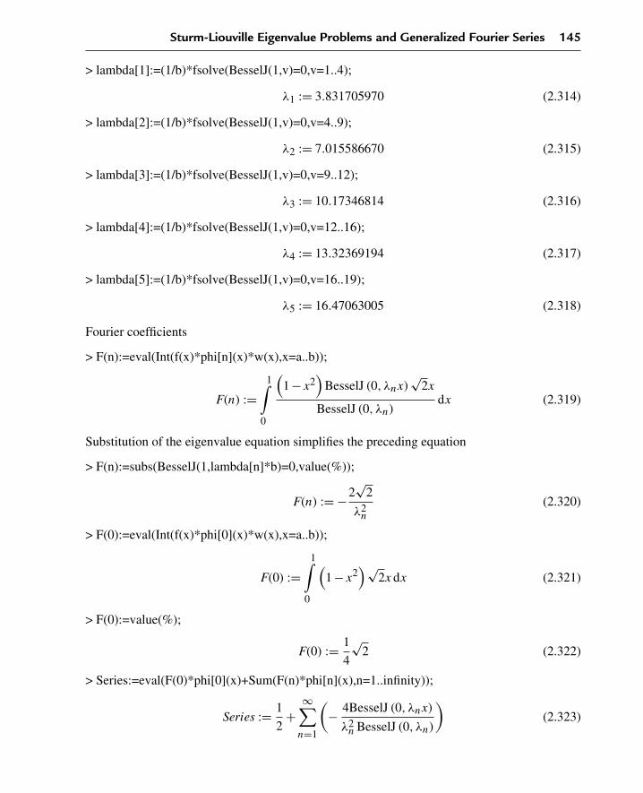
Sturm-Liouville Eigenvalue Problems and Generalized Fourier Series 145
> lambda[1]:=(1/b)*fsolve(BesselJ(1,v)=0,v=1..4);
λ1 := 3.831705970 (2.314)
> lambda[2]:=(1/b)*fsolve(BesselJ(1,v)=0,v=4..9);
λ2 := 7.015586670 (2.315)
> lambda[3]:=(1/b)*fsolve(BesselJ(1,v)=0,v=9..12);
λ3 := 10.17346814 (2.316)
> lambda[4]:=(1/b)*fsolve(BesselJ(1,v)=0,v=12..16);
λ4 := 13.32369194 (2.317)
> lambda[5]:=(1/b)*fsolve(BesselJ(1,v)=0,v=16..19);
λ5 := 16.47063005 (2.318)
Fourier coefficients
> F(n):=eval(Int(f(x)*phi[n](x)*w(x),x=a..b));
F(n) :=1∫
0
(1−x2
)BesselJ (0, λnx)
√2x
BesselJ (0, λn)dx (2.319)
Substitution of the eigenvalue equation simplifies the preceding equation
> F(n):=subs(BesselJ(1,lambda[n]*b)=0,value(%));
F(n) := −2√
2
λ2n
(2.320)
> F(0):=eval(Int(f(x)*phi[0](x)*w(x),x=a..b));
F(0) :=1∫
0
(1−x2
)√2xdx (2.321)
> F(0):=value(%);
F(0) := 1
4
√2 (2.322)
> Series:=eval(F(0)*phi[0](x)+Sum(F(n)*phi[n](x),n=1..infinity));
Series := 1
2+
∞∑n=1
(− 4BesselJ (0, λnx)
λ2n BesselJ (0, λn)
)(2.323)

146 Chapter 2
First five terms in the expansion
> Series:=F(0)*phi[0](x)+sum(F(n)*phi[n](x),n=1..5):
> plot({Series,f(x)},x=a..b,thickness=10);
x0 0.2 0.4 0.6 0.8 1
0
0.2
0.4
0.6
0.8
1
Figure 2.21
The two curves in Figure 2.21 depict the function f(x) and its Fourier series expansionapproximation in terms of the Bessel functions of the first kind of order zero, which satisfy thegiven boundary conditions. Note that f(x) satisfies the given boundary condition at the left butfails to do so at the right end point.
Chapter Summary
Sturm-Liouville operator acting on y(x)
L(y) = D(p(x)D(y))+q(x)y
The Sturm-Liouville differential equation
L(ϕ)+λw(x)ϕ = 0
Regular homogeneous boundary conditions
κ1ϕ(a)+κ2ϕx(a) = 0
and
κ3ϕ(b)+κ4ϕx(b) = 0
Generalized Fourier series expansion
f(x) =∞∑
n=0
F(n)ϕn(x)

Sturm-Liouville Eigenvalue Problems and Generalized Fourier Series 147
Statement of orthonormality with respect to the weight function w(x)
b∫a
φn(x)φm(x)w(x)dx = δ(n,m)
Generalized Fourier coefficients
F(n) =b∫
a
f(x)φn(x)w(x)dx
The generalized Fourier series expansions above are based on the orthonormalizedeigenfunction solutions to Sturm-Liouville boundary value problems. These generalized seriesexpansions will play an important role in the solutions to boundary value problems in partialdifferential equations.
Exercises
2.1. From Section 2.2, any second-order linear differential equation of the form
a2(x)
(d2
dx2y(x)
)+a1(x)
(d
dxy(x)
)+a0(x)y(x) = 0
can be converted into self-adjoint form by multiplying by the integrating factor
r(x) = e
∫a1(x)
a2(x)dx
a2(x)
Consider the following differential equations shown below. In all cases, evaluate theintegrating factor, identify p(x), q(x), and the weight function w(x), and rewrite theequations in the Sturm-Liouville (self-adjoint) form
(D(p(x)D)+q(x)+λw(x))y(x) = 0
(a) The Euler equation
d2
dx2y(x)+λy(x) = 0
(b) The Cauchy-Euler equation
x2
(d2
dx2y(x)
)+x
(d
dxy(x)
)+λy(x) = 0

148 Chapter 2
(c) The Laguerre equation from quantum mechanics
x
(d2
dx2y(x)
)+ (1−x)
(d
dxy(x)
)+λy(x) = 0
(d) The Hermite equation from quantum mechanics
d2
dx2y(x)−2x
(d
dxy(x)
)+2λy(x) = 0
(e) The Tchebycheff equation
(1−x2)
(d2
dx2y(x)
)−x
(d
dxy(x)
)+λy(x) = 0
(f) The Bessel differential equation of order m
x2
(d2
dx2y(x)
)+x
(d
dxy(x)
)−m2y(x)+λ2x2y(x) = 0
In the following problems, you will be asked to generate a set of eigenfunctions for aSturm-Liouville problem over an interval I with a particular set of boundary conditions.You are also asked to develop a generalized Fourier series expansion for three functionsover the interval. The first, f1(x), should not satisfy any of the boundary conditions.The second, f2(x), should satisfy one of the boundary conditions (left or right). Thethird, f3(x), should satisfy both boundary conditions (left and right). Pay particularattention to the quality of the convergence of each of the series depending on theboundary condition behavior of the particular function f(x) over that interval.
For problems 2.2 through 2.21, you are asked to do the following:
(a) Evaluate the eigenvalues and corresponding eigenfunctions.(b) Normalize the eigenfunctions with the respective weight function.(c) Write out the statement of orthonormality.(d) Write out the generalized Fourier series expansion for function f(x).(e) Write out the integral for the Fourier coefficients F(n).
2.2. Consider the Sturm-Liouville problem with the Euler operator over the intervalI = {x |0 < x < 1}.
d2
dx2ϕ(x)+λϕ(x) = 0
with boundary conditions
ϕ(0) = 0, ϕ(1) = 0

Sturm-Liouville Eigenvalue Problems and Generalized Fourier Series 149
Evaluate the generalized Fourier series expansion for the following:
f1(x) = 1
f2(x) = x
f3(x) = x(1−x)
With the first five terms in each series above, generate the curve of f(x) and itscorresponding series on the same set of axes.
2.3. Consider the Sturm-Liouville problem with the Euler operator over the intervalI = {x |0 < x < 1}.
d2
dx2ϕ(x)+λϕ(x) = 0
with boundary conditions
ϕ(0) = 0, ϕx(1) = 0
Evaluate the generalized Fourier series expansion for the following:
f1(x) =(
x− 1
2
)2
f2(x) = x
f3(x) = x(
1− x
2
)With the first five terms in each preceding series, generate the curve of f(x) and itscorresponding series on the same set of axes.
2.4. Consider the Sturm-Liouville problem with the Euler operator over the intervalI = {x |0 < x < 1}.
d2
dx2ϕ(x)+λϕ(x) = 0
with boundary conditions
ϕx(0) = 0, ϕ(1) = 0
Evaluate the generalized Fourier series expansion for the following:
f1(x) = x
f2(x) = 1
f3(x) = 1−x2
150 Chapter 2
With the first five terms in each series above, generate the curve of f(x) and itscorresponding series on the same set of axes.
2.5. Consider the Sturm-Liouville problem with the Euler operator over the intervalI = {x |0 < x < 1}.
d2
dx2ϕ(x)+λϕ(x) = 0
with boundary conditions
ϕx(0) = 0, ϕx(1) = 0
Evaluate the generalized Fourier series expansion for the following:
f1(x) = x
f2(x) = 1−x2
f3(x) = x2(
1− 2x
3
)
With the first five terms in each series above, generate the curve of f(x) and itscorresponding series on the same set of axes.
2.6. Consider the Sturm-Liouville problem with the Euler operator over the intervalI = {x |0 < x < 1}.
d2
dx2ϕ(x)+λϕ(x) = 0
with boundary conditions
ϕ(0) = 0, ϕx(1)+ϕ(1) = 0
Evaluate the generalized Fourier series expansion for the following:
f1(x) = 1
f2(x) = x
f3(x) = x
(1− 2x
3
)
With the first five terms in each series above, generate the curve of f(x) and itscorresponding series on the same set of axes.
2.7. Consider the Sturm-Liouville problem with the Euler operator over the intervalI = {x |0 < x < 1}.
d2
dx2ϕ(x)+λϕ(x) = 0

Sturm-Liouville Eigenvalue Problems and Generalized Fourier Series 151
with boundary conditions
ϕx(0)−ϕ(0) = 0, ϕ(1) = 0
Evaluate the generalized Fourier series expansion for the following:
f1(x) = 1
f2(x) = 1−x
f3(x) = −2x2
3+ x
3+ 1
3
With the first five terms in each preceding series, generate the curve of f(x) and itscorresponding series on the same set of axes.
2.8. Consider the Sturm-Liouville problem with the Euler operator over the intervalI = {x |0 < x < 1}.
d2
dx2ϕ(x)+λϕ(x) = 0
with boundary conditions
ϕx(0) = 0, ϕx(1)+ϕ(1) = 0
Evaluate the generalized Fourier series expansion for the following:
f1(x) = x
f2(x) = 1
f3(x) = 1− x2
3
With the first five terms in each preceding series, generate the curve of f(x) and itscorresponding series on the same set of axes.
2.9. Consider the Sturm-Liouville problem with the Euler operator over the intervalI = {x |0 < x < 1}.
d2
dx2ϕ(x)+λϕ(x) = 0
with boundary conditions
ϕx(0)−ϕ(0) = 0, ϕx(1) = 0

152 Chapter 2
Evaluate the generalized Fourier series expansion for the following:
f1(x) = x
f2(x) = 1
f3(x) = −(x−1)2
3+1
With the first five terms in each preceding series, generate the curve of f(x) and itscorresponding series on the same set of axes.
2.10. Consider the Sturm-Liouville problem with the Cauchy-Euler operator over the intervalI = {x |1 < x < 2}.
x2
(d2
dx2ϕ(x)
)+x
(d
dxϕ(x)
)+λϕ(x) = 0
with boundary conditions
ϕ(1) = 0, ϕ(2) = 0
Evaluate the generalized Fourier series expansion for the following:
f1(x) = 1
f2(x) = x−1
f3(x) = (x−1)(2−x)
With the first five terms in each preceding series, generate the curve of f(x) and itscorresponding series on the same set of axes.
2.11. Consider the Sturm-Liouville problem with the Cauchy-Euler operator over the intervalI = {x |1 < x < 2}.
x2
(d2
dx2ϕ(x)
)+x
(d
dxϕ(x)
)+λϕ(x) = 0
with boundary conditions
ϕx(1) = 0, ϕ(2) = 0
Evaluate the generalized Fourier series expansion for the following:
f1(x) = x−1
f2(x) = 1
f3(x) = x(2−x)

Sturm-Liouville Eigenvalue Problems and Generalized Fourier Series 153
With the first five terms in each preceding series, generate the curve of f(x) and itscorresponding series on the same set of axes.
2.12. Consider the Sturm-Liouville problem with the Cauchy-Euler operator over the intervalI = {x |1 < x < 2}.
x2
(d2
dx2ϕ(x)
)+x
(d
dxϕ(x)
)+λϕ(x) = 0
with boundary conditions
ϕ(1) = 0, ϕx(2) = 0
Evaluate the generalized Fourier series expansion for the following:
f1(x) =(
x− 3
2
)2
f2(x) = x−1
f3(x) = (x−1)(3−x)
2
With the first five terms in each preceding series, generate the curve of f(x) and itscorresponding series on the same set of axes.
2.13. Consider the Sturm-Liouville problem with the Cauchy-Euler operator over the intervalI = {x |1 < x < 2}.
x2
(d2
dx2ϕ(x)
)+x
(d
dxϕ(x)
)+λϕ(x) = 0
with boundary conditions
ϕx(1) = 0, ϕx(2) = 0
Evaluate the generalized Fourier series expansion for the following:
f1(x) = x−1
f2(x) = x(2−x)
f3(x) = 3x2 − 2x2
3−4x+ 5
3
With the first five terms in each preceding series, generate the curve of f(x) and itscorresponding series on the same set of axes.

154 Chapter 2
2.14. Consider the Sturm-Liouville problem with the Cauchy-Euler operator over the intervalI = {x |1 < x < 2}.
x2
(d2
dx2ϕ(x)
)+x
(d
dxϕ(x)
)+λϕ(x) = 0
with boundary conditions
ϕ(1) = 0, ϕx(2)+ϕ(2) = 0
Evaluate the generalized Fourier series expansion for the following:
f1(x) = 1
f2(x) = x−1
f3(x) = (x−1)(5−2x)
3
With the first five terms in each preceding series, generate the curve of f(x) and itscorresponding series on the same set of axes.
2.15. Consider the Sturm-Liouville problem with the Cauchy-Euler operator over the intervalI = {x |1 < x < 2}.
x2
(d2
dx2ϕ(x)
)+x
(d
dxϕ(x)
)+λϕ(x) = 0
with boundary conditions
ϕx(1)−ϕ(1) = 0, ϕ(2) = 0
Evaluate the generalized Fourier series expansion for the following:
f1(x) = 1
f2(x) = 2−x
f3(x) = −2x2
3+ 5x
3− 2
3
With the first five terms in each preceding series, generate the curve of f(x) and itscorresponding series on the same set of axes.
2.16. Consider the Sturm-Liouville problem with the Cauchy-Euler operator over the intervalI = {x |1 < x < 2}.
x2
(d2
dx2ϕ(x)
)+x
(d
dxϕ(x)
)+λϕ(x) = 0

Sturm-Liouville Eigenvalue Problems and Generalized Fourier Series 155
with boundary conditions
ϕx(1) = 0, ϕx(2)+ϕ(2) = 0
Evaluate the generalized Fourier series expansion for the following:
f1(x) = x−1
f2(x) = 1
f3(x) = 2
3− x2
3+ 2x
3
With the first five terms in each preceding series, generate the curve of f(x) and itscorresponding series on the same set of axes.
2.17. Consider the Sturm-Liouville problem with the Cauchy-Euler operator over the intervalI = {x |1 < x < 2}.
x2
(d2
dx2ϕ(x)
)+x
(d
dxϕ(x)
)+λϕ(x) = 0
with boundary conditions
ϕx(1)−ϕ(1) = 0, ϕx(2) = 0
Evaluate the generalized Fourier series expansion for the following:
f1(x) = x−1
f2(x) = 1
f3(x) = −x2
3+ 4x
3− 1
3
With the first five terms in each preceding series, generate the curve of f(x) and itscorresponding series on the same set of axes.
2.18. Consider the Sturm-Liouville problem with the Euler operator over the intervalI = {x | −1 < x < 1}.
d2
dx2ϕ(x)+λϕ(x) = 0
with periodic boundary conditions
ϕ(−1) = ϕ(1), ϕx(−1) = ϕx(1)

156 Chapter 2
Evaluate the generalized Fourier series expansion for the following:
f1(x) = x
f2(x) = 1−x2
f(3) = |x|With the first five terms in each preceding series, generate the curve of f(x) and itscorresponding series on the same set of axes.
2.19. Consider the Sturm-Liouville problem with the Bessel operator of order zero over theinterval I = {x |0 < x < 1}.
x2
(d2
dx2ϕ(x)
)+x
(d
dxϕ(x)
)+λ2x2ϕ(x) = 0
with boundary conditions
ϕ(0) < ∞, ϕ(1) = 0
Evaluate the generalized Fourier series expansion for the following:
f1(x) = x2
f2(x) = 1
f3(x) = 1−x2
With the first five terms in each preceding series, generate the curve of f(x) and itscorresponding series on the same set of axes.
2.20. Consider the Sturm-Liouville problem with the Bessel operator of order zero over theinterval I = {x |0 < x < 1}.
x2
(d2
dx2ϕ(x)
)+x
(d
dxϕ(x)
)+λ2x2ϕ(x) = 0
with boundary conditions
|ϕ(0)| < ∞, ϕx(1) = 0
Evaluate the generalized Fourier series expansion for the following:
f1(x) = 1
f2(x) = x2
f3(x) = x2 − x4
2

Sturm-Liouville Eigenvalue Problems and Generalized Fourier Series 157
With the first five terms in each preceding series, generate the curve of f(x) and itscorresponding series on the same set of axes.
2.21. Consider the Sturm-Liouville problem with the Bessel operator of order zero over theinterval I = {x |0 < x < 1}.
x2
(d2
dx2ϕ(x)
)+x
(d
dxϕ(x)
)+λ2x2ϕ(x) = 0
with boundary conditions
|ϕ(0)| < ∞, ϕx(1)+ϕ(1) = 0
Evaluate the generalized Fourier series expansion for the following:
f1(x) = 1
f2(x) = x2
f3(x) = 1− x2
3
With the first five terms in each preceding series, generate the curve of f(x) and itscorresponding series on the same set of axes.
2.22. Consider the non-self-adjoint boundary value problem
d2
dx2y(x)+4
(d
dxy(x)
)+ (4+9λ)y(x) = 0
with boundary conditions
y(0) = 0, y(1) = 0
(a) Transform into the self-adjoint form and identify the weight function w(x).(b) Solve for the eigenvalues and the corresponding eigenfuctions.(c) Normalize the eigenfunctions and write out the statement of orthonormality.(d) Evaluate the generalized Fourier series expansion of the function f(x) = x−x2
over the interval I = {x |0 < x < 1}.2.23. Consider the non-self-adjoint boundary value problem
d2
dx2y(x)+2
(d
dxy(x)
)+ (1−λ)y(x) = 0
with boundary conditions
y(0) = 0, y(1) = 0

158 Chapter 2
(a) Transfer into the self-adjoint form and identify the weight function w(x).(b) Solve for the eigenvalues and the corresponding eigenfuctions.(c) Normalize the eigenfunctions and write out the statement of orthonormality.(d) Evaluate the generalized Fourier series expansion of the function f(x) = 1−x
over the interval I = {x |0 < x < 1}.
The Rayleigh Quotient
The Rayleigh quotient is useful in determining the sign of the eigenvalues. It can be derivedfrom the expanded form of the Sturm-Liouville equation:
(d
dxp(x)
)(d
dxϕ(x)
)+p(x)
(d2
dx2ϕ(x)
)+q(x)ϕ(x)+λw(x)ϕ(x) = 0
If we multiply both sides of the above by ϕ(x) and integrate over the intervalI = {x |a < x < b}, we get
b∫a
(ϕ(x)
((d
dxp(x)
)(d
dxϕ(x)
)+p(x)
(d2
dx2ϕ(x)
))+q(x)ϕ(x)2
)dx
+λ
(∫ b
aϕ(x)2w(x)dx
)= 0
Integrating by parts and solving for λ, we get
λ =−p(b)ϕ(b)ϕx(b)+p(a)ϕ(a)ϕx(a)+
∫ b
a
(p(x)
(d
dxϕ(x)
)2−q(x)ϕ(x)2
)dx
∫ b
aϕ(x)2w(x)dx
We recognize the denominator here to be the norm of the eigenfunction. It is obvious that if thefollowing conditions hold
0 ≤ −p(b)ϕ(b)ϕx(b)+p(a)ϕ(a)ϕx(a)
in addition to
0 ≤ p(x) and q(x) ≤ 0
then the term on the right-hand side must be positive or equal to zero; thus, the eigenvalues λ
must be greater than or equal to zero—that is, there are no negative eigenvalues. We tookadvantage of this earlier when we evaluated the eigenvalues in the example problems.

Sturm-Liouville Eigenvalue Problems and Generalized Fourier Series 159
2.24. For the Sturm-Liouville problems 2.7 through 2.9 for the Euler operator, identify q(x)
and p(x) and show that for the given boundary conditions, we have 0 ≤ λ.
2.25. For the Sturm-Liouville problems 2.15 through 2.17 for the Cauchy-Euler operator,identify q(x) and p(x) and show that for the given boundary conditions, we have 0 ≤ λ.
2.26. For the Sturm-Liouville problems 2.19 through 2.20 for the Bessel operator, identifyq(x) and p(x) and show that for the given boundary conditions, we have 0 ≤ λ.
Statement of Orthogonality
From Section 2.3, we showed that for the Sturm-Liouville operator
L = D(p(x)D)+q(x)
acting upon two functions u(x) and v(x) over the interval I = {x |a < x < b}, Green’s formulareads∫ b
a(uL(v)−vL(u))dx = p(b) (u(b)vx(b)−v(b)ux(b))−p(a) (u(a)vx(a)−v(a)ux(a))
If ϕn(x) and ϕm(x) are both solutions to the Sturm-Liouville differential equations
Lϕm(x)+λmw(x)ϕm(x) = 0
Lϕn(x)+λnw(x)ϕn(x) = 0
then it can be shown that for regular boundary conditions, the right-hand side of Green’sformula vanishes and we get
(λn −λm)
(∫ b
aϕn(x)ϕm(x)w(x)dx
)= 0
For λm �= λn, the preceding is the equivalent statement of orthogonality of the eigenfunctionswith respect to the weight function w(x). In the following exercises, you are asked to considerthe specific boundary conditions for the given problem and to show that the right-hand side ofGreen’s formula does indeed reduce to zero.
2.27. Consider Exercise 2.4. Show that for the given boundary conditions, the right-hand sideof Green’s formula vanishes, thus establishing the orthogonality of the eigenfunctions.
2.28. Consider Exercise 2.6. Show that for the given boundary conditions, the right-hand sideof Green’s formula vanishes, thus establishing the orthogonality of the eigenfunctions.
2.29. Consider Exercise 2.10. Show that for the given boundary conditions, the right-handside of Green’s formula vanishes, thus establishing the orthogonality of theeigenfunctions.

160 Chapter 2
2.30. Consider Exercise 2.12. Show that for the given boundary conditions, the right-handside of Green’s formula vanishes, thus establishing the orthogonality of theeigenfunctions.
2.31. Consider Exercise 2.14. Show that for the given boundary conditions, the right-handside of Green’s formula vanishes, thus establishing the orthogonality of theeigenfunctions.
2.32. Consider Exercise 2.18. Show that for the given periodic boundary conditions, theright-hand side of Green’s formula vanishes, thus establishing the orthogonality of theeigenfunctions.
2.33. Consider Exercise 2.19. Show that for the given boundary conditions, the right-handside of Green’s formula vanishes, thus establishing the orthogonality of theeigenfunctions.
2.34. Consider Exercise 2.20. Show that for the given boundary conditions, the right-handside of Green’s formula vanishes, thus establishing the orthogonality of theeigenfunctions.

CHAPTER 3
The Diffusion or Heat PartialDifferential Equation
3.1 Introduction
We begin by examining types of partial differential equations that occur in describing heat ordiffusion phenomena. Heat or diffusion phenomena are treated similarly, since physicists likenthe random motion of molecules under nonuniform temperature distributions to be the same asthe diffusion of molecules under nonuniform concentration.
The partial differential equations that we examine here are said to be linear in that the partialdifferential operator obeys the defining characteristics of a linear operator. The operator L isdefined to be linear if it satisfies the following, where C1 and C2 are constants:
L(C1u1+C2u2) = C1L(u)+C2L(u2)
We examine the following partial differential equations that have linear operators. We shall seethat many of the results of Chapters 1 and 2 will play an important role in the results of thischapter.
3.2 One-Dimensional Diffusion Operator in RectangularCoordinates
It can be shown that heat or diffusion phenomena in one dimension can be described by thefollowing partial differential equation in the rectangular coordinate system:
c(x)ρ(x)
(∂
∂tu(x, t)
)=
(d
dxK(x)
)(∂
∂xu(x, t)
)+K(x)
(∂2
∂x2u(x, t)
)+q(x, t)
where, for the situation of heat phenomena, u(x, t) denotes the spatial-time dependenttemperature, K(x) denotes the thermal conductivity, c(x) denotes the specific heat, ρ(x) denotesthe mass density of the medium, and q(x, t) denotes the time rate of the input source heat
© 2009, 2003, 1999 Elsevier Inc. 161

162 Chapter 3
density into the medium. If the medium is uniform, then the coefficients are spatially invariant,and we can write them as constants. For constant coefficients, the preceding simplifies to
∂
∂tu(x, t) = k
(∂2
∂x2u(x, t)
)+h(x, t)
where k, the thermal diffusivity of the medium, and h(x, t) are given as
k = K
cρ
and
h(x, t) = q(x, t)
cρ
We can write the preceding partial differential equation in terms of the linear heat or diffusionoperator as
L(u) = h(x, t)
where the diffusion operator in rectangular coordinates reads
L(u) = ∂
∂tu(x, t)−k
(∂2
∂x2u(x, t)
)
If h(x, t) = 0, then there are no heat sources in the system and this nonhomogeneous partialdifferential equation reduces to its corresponding homogeneous equation
L(u) = 0
This homogeneous equation can be written in the more familiar form
∂
∂tu(x, t) = k
(∂2
∂x2u(x, t)
)
This partial differential equation for diffusion or heat phenomena is characterized by the factthat it relates the first partial derivative with respect to the time variable with the second partialderivative with respect to the spatial variable.
Some motivation for the derivation of this equation can be provided in terms of some simpleconcepts from introductory calculus. Recall that the slope of a curve is found from the firstderivative and the concavity of the curve is found from the second derivative with respect tothe spatial variable x. In addition, the time rate of change, or speed, is given as the firstderivative with respect to the time variable t.
We imagine the sideview profile of a dome-shaped pile of dry beach sand on a flat surfacewhile it undergoes settling or diffusion. We let u(x, t) denote the time and spatial dependent

The Diffusion or Heat Partial Differential Equation 163
height of the pile of sand. For a typical sandpile—as the sand is being poured from a pail—theprofile is concave down; thus, the second derivative with respect to the spatial variable isnegative. As the sand settles from a peak, the concavity goes to zero; the speed of diffusion, orsettling, of the pile height is negative; and the speed of drop of the pile height lessens as thepile gets flatter. Thus, the time-rate of change (speed) of the profile height is proportional to thespatial concavity of the profile, the identical behavior described by the preceding partialdifferential equation.
A typical diffusion problem reads as follows. We seek the temperature distribution u(x, t) in athin uniform rod over the finite interval I = {x |0 < x < 1}. The lateral surface of the rod isinsulated, so no heat can escape from the sides of the rod. Both the left and right ends of the rodare held at a fixed temperature of zero. The initial temperature distribution in the rod is given asu(x,0) = f(x). There are no external heat sources, and the thermal diffusivity of the rod isk = 1/10.
The homogeneous diffusion equation for this problem reads
∂
∂tu(x, t) =
∂2
∂x2 u(x, t)
10
Since both ends of the rod are at a fixed temperature of zero, the boundary conditions are type 1at x = 0 and type 1 at x = 1:
u(0, t) = 0 and u(1, t) = 0
The initial condition is
u(x,0) = f(x)
We will solve this specific problem later. For now, we develop the generalized procedure forthe solution to this homogeneous partial differential equation over a finite domain withhomogeneous boundary conditions using the method of separation of variables.
3.3 Method of Separation of Variables for the DiffusionEquation
The homogeneous diffusion equation for a uniform system in one dimension in rectangularcoordinates is rewritten as
∂
∂tu(x, t) = k
(∂2
∂x2u(x, t)
)

164 Chapter 3
Generally, one seeks a solution to this problem over the finite one-dimensional domainI = {x |a < x < b} subject to the regular homogeneous boundary conditions
κ1u(a, t)+κ2ux(a, t) = 0
and
κ3u(b, t)+κ4ux(b, t) = 0
and the initial condition
u(x,0) = f(x)
In the method of separation of variables, the character of the equation is such that we canassume a solution in the form of a product as follows:
u(x, t) = X(x)T(t)
Since the two independent variables in the partial differential equation are the spatial variable x
and the time variable t, then the preceding assumed solution is written as a product of twofunctions: one that is exclusively a function of x and one that is an exclusive function of t.
Substituting this assumed solution into the partial differential equation yields
X(x)
(d
dtT(t)
)= k
(d2
dx2X(x)
)T(t)
Dividing both sides of this equation by the product solution gives
ddt
T(t)
kT(t)=
d2
dx2 X(x)
X(x)
Because the left-hand side is an exclusive function of t and the right-hand side an exclusivefunction of x, and x and t are independent, then the only way this can hold for all values of x
and t is to set each side equal to a constant. Doing so, we get the following two ordinarydifferential equations in terms of the separation constant λ:
d
dtT(t)+kλT(t) = 0
and
d2
dx2X(x)+λX(x) = 0
The preceding differential equation in t is an ordinary first-order linear homogeneousdifferential equation for which we already have the solution from Section 1.2. The second

The Diffusion or Heat Partial Differential Equation 165
differential equation in x is an ordinary second-order linear homogeneous equation for whichwe already have the solution from Section 1.4.
If we substitute the spatial boundary conditions into the assumed solution, we get
κ1X(a)T(t)+κ2Xx(a)T(t) = 0
and
κ3X(b)T(t)+κ4Xx(b)T(t) = 0
If the preceding condition is to hold for all times t, then the spatial function X(x) mustindependently satisfy the boundary conditions.
3.4 Sturm-Liouville Problem for the Diffusion Equation
The second differential equation in the spatial variable x just given must be solved subject tothe homogeneous spatial boundary conditions over the finite interval. The Sturm-Liouvilleproblem for the diffusion equation consists of the ordinary differential equation
d2
dx2X(x)+λX(x) = 0
along with the corresponding regular homogeneous boundary conditions, which read
κ1X(a)+κ2Xx(a) = 0
and
κ3X(b)+κ4Xx(b) = 0
We see this problem in the spatial variable x to be a “regular” Sturm-Liouville eigenvalueproblem where the allowed values of λ are called the system “eigenvalues” and thecorresponding solutions are called the “eigenfunctions.” Note that the preceding ordinarydifferential equation is of the Euler type, and the weight function is w(x) = 1.
From Section 2.1, it was noted that for regular Sturm-Liouville problems over finite domains,there exists an infinite number of eigenvalues that can be indexed by the positive integers n.The indexed eigenvalues and corresponding eigenfunctions are given, respectively, as
λn,Xn(x)
for n = 0,1,2,3, . . . .

166 Chapter 3
The eigenfunctions form a “complete” set with respect to any piecewise smooth function overthe finite interval I = {x |a < x < b}. Further, the eigenfunctions can be normalized and thecorresponding statement of orthonormality reads
b∫a
Xn(x)Xm(x)dx = δ(n,m)
where the term on the right is the familiar Kronecker delta function, which was defined inSection 2.2. We now focus on the solution to the time-dependent differential equation, whichreads
d
dtT(t)+kλT(t) = 0
From Section 1.2 on linear first-order differential equations, the solution to this time-dependentdifferential equation in terms of the allowed eigenvalues is
Tn(t) = C(n)e−kλnt
where the coefficients C(n) are unknown arbitrary constants.
By the method of separation of variables, we arrive at an infinite number of indexed solutionsun(x, t) (n = 0,1,2,3, . . .) for the homogeneous diffusion partial differential equation, over afinite interval, given as
un(x, t) = Xn(x)C(n)e−kλnt
Because the differential operator is linear, then any superposition of solutions to thehomogeneous equation is also a solution to the problem. Thus, we can write the generalsolution to the homogeneous partial differential equation as the infinite sum
u(x, t) =∞∑
n=0
Xn(x)C(n)e−kλnt
This equation is the eigenfunction expansion form of the solution to the diffusion partialdifferential equation. The terms of its sum are the “basis vectors” of the solution space of thepartial differential equation. Thus, for the diffusion partial differential equation, there are aninfinite number of basis vectors in the solution space and we say the dimension of the solutionspace is infinite. This compares dramatically with an ordinary differential equation wherebythe dimension of the solution space is finite and equal to the order of the equation.
We demonstrate the discussed concepts with the example diffusion problem in rectangularcoordinates given in Section 3.2.
DEMONSTRATION: We seek the temperature distribution u(x, t) in a thin uniform rod overthe finite interval I = {x |0 < x < 1}. The lateral surface of the rod is insulated. Both the left

The Diffusion or Heat Partial Differential Equation 167
and right ends of the rod are held at a fixed temperature of zero. The initial temperaturedistribution in the rod is given as f(x). There are no external heat sources, and the thermaldiffusivity of the rod is k = 1/10.
SOLUTION: The homogeneous diffusion equation for this problem reads
∂
∂tu(x, t) =
∂2
∂x2 u(x, t)
10
Since both ends of the rod are at a fixed temperature of zero, the boundary conditions are type 1at x = 0 and type 1 at x = 1.
u(0, t) = 0 and u(1, t) = 0
The initial condition is
u(x,0) = f(x)
From the method of separation of variables, we obtain the two ordinary differential equations
d
dtT(t)+ λT(t)
10= 0
and
d2
dx2X(x)+λX(x) = 0
We first consider the spatial differential equation in x. This is an Euler-type differentialequation with type 1 conditions at x = 0 and at x = 1:
X(0) = 0 and X(1) = 0
This same problem was considered in Example 2.5.1 in Chapter 2. The allowed eigenvaluesand corresponding orthonormal eigenfunctions were evaluated as
λn = n2π2
and
Xn(x) = √2 sin(nπx)
for n = 1,2,3, . . . .
The corresponding statement of orthonormality with respect to the weight function w(x) = 1over the interval I is
1∫0
2 sin(nπx) sin(mπx)dx = δ(n,m)

168 Chapter 3
When solving boundary value problems, the first choice of differential equation to be solved isgenerally the spatial differential equation. The reason for this is that the spatial equation, alongwith the spatial boundary conditions, determines the character of the system eigenvalues.These eigenvalues must be known before we can get a complete solution to the time-dependentdifferential equation.
We now consider the solution to the time-dependent differential equation. This is a first-orderordinary differential equation, which we solved in Section 1.2. The solution, for the allowedvalues of λ given earlier, reads
Tn(t) = C(n)e− n2π2t10
Thus, the eigenfunction expansion for the solution to the problem reads
u(x, t) =∞∑
n=1
C(n)e− n2π2t10
√2 sin(nπx)
The unknown coefficients C(n) for n = 1,2,3, . . . are to be determined from the initialcondition function that is imposed on the problem.
3.5 Initial Conditions for the Diffusion Equation inRectangular Coordinates
We now consider the initial conditions on the problem. Suppose that, at time t = 0, the rod hasan initial temperature distribution
u(x,0) = f(x)
Substituting this into the following general solution
u(x, t) =∞∑
n=0
Xn(x)C(n)e−kλnt
at time t = 0 yields
f(x) =∞∑
n=0
Xn(x)C(n)
Since the eigenfunctions of the regular Sturm-Liouville problem form a complete set withrespect to piecewise smooth functions over the finite interval I, then the preceding is thegeneralized Fourier series expansion of the function f(x) in terms of the eigenfunctions. Theterms C(n) are the corresponding Fourier coefficients. We now evaluate these coefficients.

The Diffusion or Heat Partial Differential Equation 169
As we did in Section 2.3 for the generalized Fourier series expansion, we take the inner productof both sides of the preceding series with respect to the weight function w(x) = 1. Assumingvalidity of the interchange between the summation and integration operations, we get
b∫a
f(x)Xm(x)dx =∞∑
n=0
C(n)
⎛⎝ b∫
a
Xm(x)Xn(x)dx
⎞⎠
Taking advantage of the statement of orthonormality, this reduces to
b∫a
f(x)Xm(x)dx =∞∑
n=0
C(n)δ(n,m)
Due to the mathematical character of the Kronecker delta function, only one term (m = n) inthe sum survives, and the preceding sum reduces to
C(m) =b∫
a
f(x)Xm(x)dx
Thus, we have evaluated the Fourier coefficients in the generalized expansion of f(x). We canwrite the final generalized solution to the diffusion equation in one dimension, subject to thegiven homogeneous boundary conditions and initial conditions, as
u(x, t) =∞∑
n=0
Xn(x)e−kλnt
⎛⎝ b∫
a
f(s)Xn(s)ds
⎞⎠
All of the previous operations are based on the assumption that the infinite series is uniformlyconvergent and that the formal interchange between the integration and the summationoperators is valid. It can be shown that if the function f(x) is piecewise smooth over theinterval I and it satisfies the same boundary conditions as the eigenfunctions, then thepreceding series is, indeed, uniformly convergent.
DEMONSTRATION: We now provide a demonstration of these concepts for the exampleproblem given in Section 3.2 for the case where the initial temperature distribution u(x,0) is
f(x) = x(1−x)
SOLUTION: From an earlier development, the unknown Fourier coefficients C(n) areevaluated from the inner product between the orthonormalized eigenfunctions and f(x) overthe interval I = {x |0 < x < 1} as shown:
C(n) =1∫
0
x(1−x)√
2 sin(nπx)dx

170 Chapter 3
Evaluation of this integral yields
C(n) = −2√
2((−1)n −1)
n3π3
for n = 1,2,3, . . . . Thus, the final series solution to the example problem reads
u(x, t) =∞∑
n=1
⎛⎝−4((−1)n −1)e
−n2π2t10 sin(nπx)
n3π3
⎞⎠
The detailed development of the solution of this problem and its graphics are given in one ofthe Maple worksheet examples given later.
The Maple worksheets given later are expressed in terms of generalized values for length,diffusivity, and initial condition function u(x,0) = f(x). The reason for the generalization is sothat the student or practitioner of the problem can change these values at will for differentapplications.
3.6 Example Diffusion Problems in RectangularCoordinates
We now consider several examples of partial differential equations for heat or diffusionphenomena under various homogeneous boundary conditions over finite, one-dimensionalintervals in the rectangular coordinate system. We note that all the spatial ordinary differentialequations are of the Euler type.
EXAMPLE 3.6.1: We seek the temperature distribution u(x, t) in a thin rod over the finiteinterval I = {x |0 < x < 1} whose lateral surface is insulated. Both the left and right ends of therod are held at a fixed temperature of zero. The initial temperature distribution f(x) is givenfollowing, and the diffusivity is k = 1/10.
SOLUTION: The homogeneous diffusion equation is
∂
∂tu(x, t) = k
(∂2
∂x2u(x, t)
)
The boundary conditions are type 1 at x = 0 and type 1 at x = 1
u(0, t) = 0 and u(1, t) = 0
The initial condition is
u(x,0) = x(1−x)
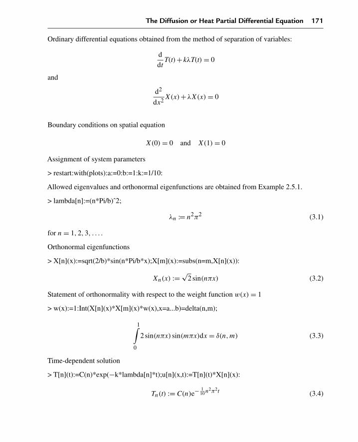
The Diffusion or Heat Partial Differential Equation 171
Ordinary differential equations obtained from the method of separation of variables:
d
dtT(t)+kλT(t) = 0
and
d2
dx2X(x)+λX(x) = 0
Boundary conditions on spatial equation
X(0) = 0 and X(1) = 0
Assignment of system parameters
> restart:with(plots):a:=0:b:=1:k:=1/10:
Allowed eigenvalues and orthonormal eigenfunctions are obtained from Example 2.5.1.
> lambda[n]:=(n*Pi/b)ˆ2;
λn := n2π2 (3.1)
for n = 1,2,3, . . . .
Orthonormal eigenfunctions
> X[n](x):=sqrt(2/b)*sin(n*Pi/b*x);X[m](x):=subs(n=m,X[n](x)):
Xn(x) := √2 sin(nπx) (3.2)
Statement of orthonormality with respect to the weight function w(x) = 1
> w(x):=1:Int(X[n](x)*X[m](x)*w(x),x=a...b)=delta(n,m);
1∫0
2 sin(nπx) sin(mπx)dx = δ(n,m) (3.3)
Time-dependent solution
> T[n](t):=C(n)*exp(−k*lambda[n]*t);u[n](x,t):=T[n](t)*X[n](x):
Tn(t) := C(n)e− 110 n2π2t (3.4)

172 Chapter 3
Eigenfunction expansion
> u(x,t):=Sum(u[n](x,t),n=1..infinity);
u(x, t) :=∞∑
n=1
C(n)e− 110 n2π2t
√2 sin(nπx) (3.5)
Evaluation of Fourier coefficients for the specific initial condition
> f(x):=x*(1−x);
f(x) := x(1−x) (3.6)
> C(n):=Int(f(x)*X[n](x)*w(x),x=a..b);C(n):=expand(value(%)):
C(n) :=1∫
0
x(1−x)√
2 sin(nπx)dx (3.7)
> C(n):=radsimp(subs({sin(n*Pi)=0,cos(n*Pi)=(−1)ˆn},C(n)));
C(n) := −2√
2(−1+ (−1)n)
n3π3(3.8)
Generalized series terms
> u[n](x,t):=eval(T[n](t)*X[n](x));
un(x, t) := −4(−1+ (−1)n)e− 110 n2π2t sin(nπx)
n3π3(3.9)
Series solution
> u(x,t):=Sum(u[n](x,t),n=1..infinity);
u(x, t) :=∞∑
n=1
(−4(−1+ (−1)n)e− 1
10 n2π2t sin(nπx)
n3π3
)(3.10)
First few terms of sum
> u(x,t):=sum(u[n](x,t),n=1..3):
ANIMATION
> animate(u(x,t),x=a..b,t=0..5,color=red,thickness=10);
The preceding animation command illustrates the spatial-time-dependent solution for u(x, t).The animation sequence shown in Figure 3.1 shows snapshots at times t = 0,1,2,3,4, and 5.

The Diffusion or Heat Partial Differential Equation 173
ANIMATION SEQUENCE
> u(x,0):=subs(t=0,u(x,t)):u(x,1):=subs(t=1,u(x,t)):> u(x,2):=subs(t=2,u(x,t)):u(x,3):=subs(t=3,u(x,t)):> u(x,4):=subs(t=4,u(x,t)):u(x,5):=subs(t=5,u(x,t)):> plot({u(x,0),u(x,1),u(x,2),u(x,3),u(x,4),u(x,5),},x=a..b,thickness=10);
x0 0.2 0.4 0.6 0.8 1
0
0.05
0.10
0.15
0.20
Figure 3.1
EXAMPLE 3.6.2: We seek the temperature distribution u(x, t) in a thin rod over the finiteinterval I = {x |0 < x < 1} whose lateral surface is insulated. The left end is at a fixedtemperature of zero and the right end is insulated. The initial temperature distribution f(x) isgiven following, and the diffusivity is k = 1/10.
SOLUTION: The homogeneous diffusion equation is
∂
∂tu(x, t) = k
(∂2
∂x2u(x, t)
)
The boundary conditions are type 1 at x = 0 and type 2 at x = 1
u(0, t) = 0 and ux(1, t) = 0
The initial condition is
u(x,0) = x− x2
2
Ordinary differential equations obtained from the method of separation of variables:
d
dtT(t)+kλT(t) = 0
and
d2
dx2X(x)+λX(x) = 0

174 Chapter 3
Boundary conditions on spatial equation
X(0) = 0 and Xx(1) = 0
Assignment of system parameters
> restart:with(plots):a:=0:b:=1:k:=1/10:
Allowed eigenvalues and orthonormal eigenfunctions are obtained from Example 2.5.2.
> lambda[n]:=((2*n−1)*Pi/(2*b))ˆ2;
λn := 1
4(2n−1)2π2 (3.11)
for n = 1,2,3, . . . .
Orthonormal eigenfunctions
> X[n](x):=sqrt(2/b)*sin((2*n−1)*Pi/(2*b)*x);X[m](x):=subs(n=m,X[n](x)):
Xn(x) := √2 sin
(1
2(2n−1)πx
)(3.12)
Statement of orthonormality with respect to the weight function w(x) = 1
> w(x):=1:Int(X[n](x)*X[m](x)*w(x),x=a..b)=delta(n,m);
1∫0
2 sin
(1
2(2n−1)πx
)sin
(1
2(2m−1)πx
)dx = δ(n,m) (3.13)
Time-dependent solution
> T[n](t):=C(n)*exp(−k*lambda[n]*t);
Tn(t) := C(n)e− 140 (2n−1)2π2t (3.14)
Generalized series terms
> u[n](x,t):=T[n](t)*X[n](x);
un(x, t) := C(n)e− 140 (2n−1)2π2t
√2 sin
(1
2(2n−1)πx
)(3.15)
Eigenfunction expansion
> u(x,t):=Sum(u[n](x,t),n=1..infinity);
u(x, t) :=∞∑
n=1
C(n)e− 140 (2n−1)2π2t
√2 sin
(1
2(2n−1)πx
)(3.16)
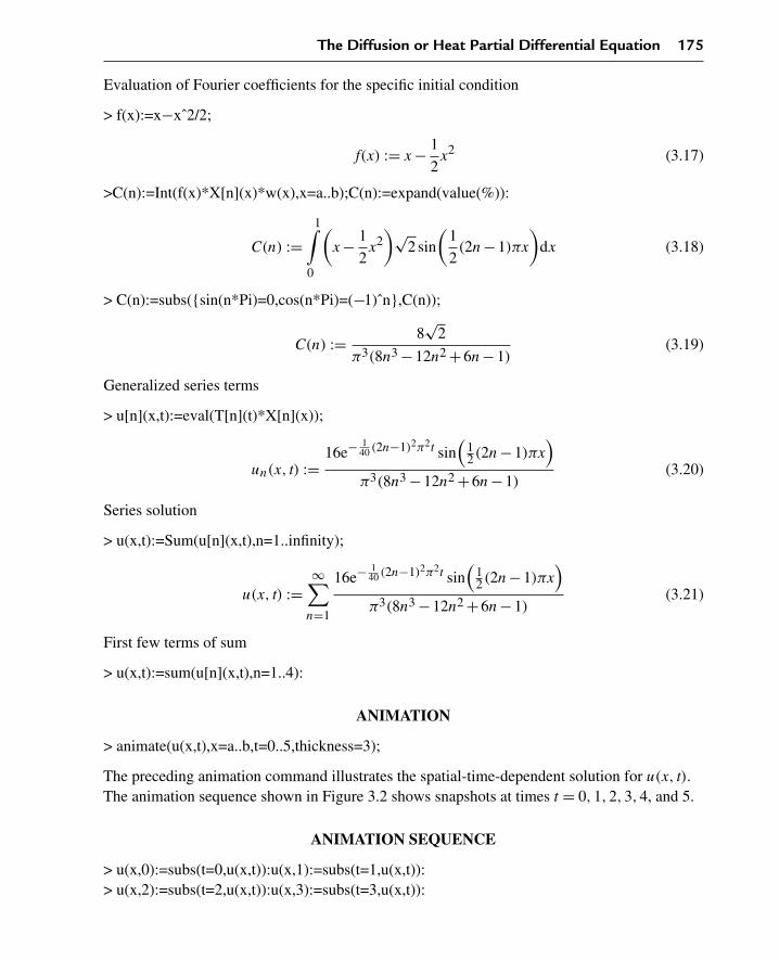
The Diffusion or Heat Partial Differential Equation 175
Evaluation of Fourier coefficients for the specific initial condition
> f(x):=x−xˆ2/2;
f(x) := x− 1
2x2 (3.17)
>C(n):=Int(f(x)*X[n](x)*w(x),x=a..b);C(n):=expand(value(%)):
C(n) :=1∫
0
(x− 1
2x2
)√2 sin
(1
2(2n−1)πx
)dx (3.18)
> C(n):=subs({sin(n*Pi)=0,cos(n*Pi)=(−1)ˆn},C(n));
C(n) := 8√
2
π3(8n3 −12n2 +6n−1)(3.19)
Generalized series terms
> u[n](x,t):=eval(T[n](t)*X[n](x));
un(x, t) :=16e− 1
40 (2n−1)2π2t sin(
12(2n−1)πx
)π3(8n3 −12n2 +6n−1)
(3.20)
Series solution
> u(x,t):=Sum(u[n](x,t),n=1..infinity);
u(x, t) :=∞∑
n=1
16e− 140 (2n−1)2π2t sin
(12(2n−1)πx
)π3(8n3 −12n2 +6n−1)
(3.21)
First few terms of sum
> u(x,t):=sum(u[n](x,t),n=1..4):
ANIMATION
> animate(u(x,t),x=a..b,t=0..5,thickness=3);
The preceding animation command illustrates the spatial-time-dependent solution for u(x, t).The animation sequence shown in Figure 3.2 shows snapshots at times t = 0,1,2,3,4, and 5.
ANIMATION SEQUENCE
> u(x,0):=subs(t=0,u(x,t)):u(x,1):=subs(t=1,u(x,t)):> u(x,2):=subs(t=2,u(x,t)):u(x,3):=subs(t=3,u(x,t)):

176 Chapter 3
> u(x,4):=subs(t=4,u(x,t)):u(x,5):=subs(t=5,u(x,t)):> plot({u(x,0),u(x,1),u(x,2),u(x,3),u(x,4),u(x,5)},x=0..b,thickness=10);
xx0 0.2 0.4 0.6 0.8 1
0.1
0.3
0.2
0.4
0
Figure 3.2
EXAMPLE 3.6.3: We again consider the temperature distribution u(x, t) in a thin rod over theinterval I = {x |0 < x < 1} whose lateral surface is insulated. Both the left and right ends of therod are insulated. The initial temperature distribution f(x) is given following, and thediffusivity is k = 1/10.
SOLUTION: The homogeneous diffusion equation is
∂
∂tu(x, t) = k
(∂2
∂x2u(x, t)
)
The boundary conditions are type 2 at x = 0 and type 2 at x = 1
ux(0, t) = 0 and ux(1, t) = 0
The initial condition is
u(x,0) = x
Ordinary differential equations obtained from the method of separation of variables
d
dtT(t)+kλT(t) = 0
and
d2
dx2X(x)+λX(x) = 0
Boundary conditions on spatial equation
Xx(0) = 0 and Xx(1) = 0

The Diffusion or Heat Partial Differential Equation 177
Assignment of system parameters
> restart:with(plots):a:=0:b:=1:k:=1/10:
Allowed eigenvalues and orthonormal eigenfunctions are obtained from Example 2.5.3.
> lambda[0]:=0;
λ0 := 0 (3.22)
for n = 0.
Orthonormal eigenfunction
> X[0](x):=1/sqrt(b);
X0(x) := 1 (3.23)
For n = 1,2,3, . . . ,
> lambda[n]:=(n*Pi/b)ˆ2;
λn := n2π2 (3.24)
Orthonormal eigenfunctions
> X[n](x):=sqrt(2/b)*cos(n*Pi/b*x);X[m](x):=subs(n=m,X[n](x)):
Xn(x) := √2 cos(nπx) (3.25)
Statement of orthonormality with respect to the weight function w(x) = 1
> w(x):=1:Int(X[n](x)*X[m](x)*w(x),x=a...b)=delta(n,m);
1∫0
2 cos(nπx) cos(mπx)dx = δ(n,m) (3.26)
Time-dependent solution
For n = 1,2,3, . . . ,
> T[n](t):=C(n)*exp(−k*lambda[n]*t);
Tn(t) := C(n)e− 110 n2π2t (3.27)
Generalized series terms
> u[n](x,t):=T[n](t)*X[n](x);
un(x, t) := C(n)e− 110 n2π2t
√2 cos(nπx) (3.28)
178 Chapter 3
For n = 0,
> T[0](t):=eval(subs(n=0,T[n](t)));u[0](x,t):=T[0](t)*X[0](x):
T0(t) := C(0) (3.29)
Eigenfunction expansion
> u(x,t):=u[0](x,t)+Sum(u[n](x,t),n=1..infinity);
u(x, t) := C(0)+∞∑
n=1
C(n)e− 110 n2π2t
√2 cos(nπx) (3.30)
Evaluation of Fourier coefficients for the specific initial condition
> f(x):=x;
f(x) := x (3.31)
> C(n):=Int(f(x)*X[n](x)*w(x),x=a..b);C(n):=expand(value(%)):
C(n) :=1∫
0
x√
2 cos(nπx)dx (3.32)
> C(n):=radsimp(subs({sin(n*Pi)=0,cos(n*Pi)=(−1)ˆn},C(n)));
C(n) :=√
2(−1+ (−1)n)
n2π2(3.33)
> C(0):=Int(f(x)*X[0](x)*w(x),x=a..b);C(0):=expand(value(%)):
C(0) :=1∫
0
xdx (3.34)
> C(0):=value(%);
C(0) := 1
2(3.35)
> u[0](x,t):=eval(T[0](t)*X[0](x));
Generalized series terms
> u[n](x,t):=eval(T[n](t)*X[n](x));
un(x, t) := 2(−1+ (−1)n) e− 110 n2π2t cos(nπx)
n2π2(3.36)
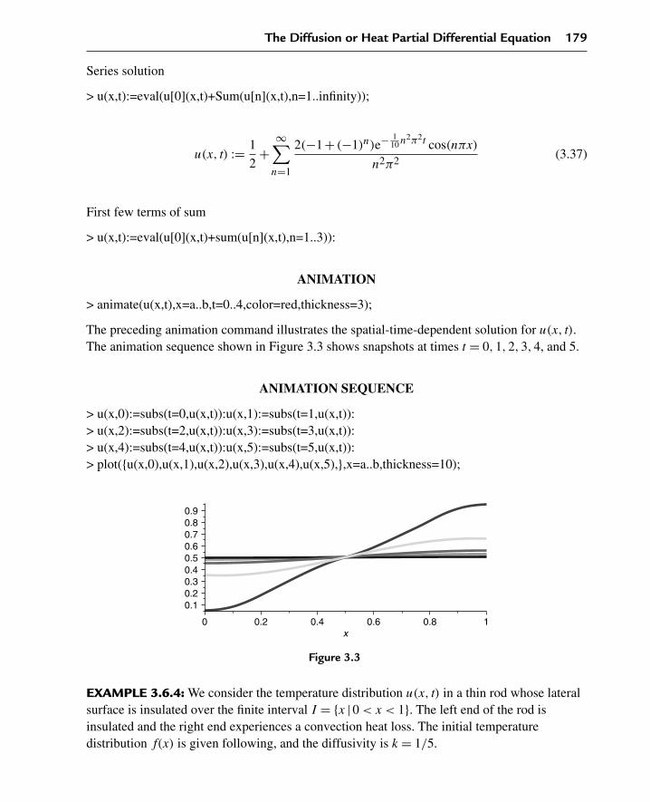
The Diffusion or Heat Partial Differential Equation 179
Series solution
> u(x,t):=eval(u[0](x,t)+Sum(u[n](x,t),n=1..infinity));
u(x, t) := 1
2+
∞∑n=1
2(−1+ (−1)n)e− 110 n2π2t cos(nπx)
n2π2(3.37)
First few terms of sum
> u(x,t):=eval(u[0](x,t)+sum(u[n](x,t),n=1..3)):
ANIMATION
> animate(u(x,t),x=a..b,t=0..4,color=red,thickness=3);
The preceding animation command illustrates the spatial-time-dependent solution for u(x, t).The animation sequence shown in Figure 3.3 shows snapshots at times t = 0,1,2,3,4, and 5.
ANIMATION SEQUENCE
> u(x,0):=subs(t=0,u(x,t)):u(x,1):=subs(t=1,u(x,t)):> u(x,2):=subs(t=2,u(x,t)):u(x,3):=subs(t=3,u(x,t)):> u(x,4):=subs(t=4,u(x,t)):u(x,5):=subs(t=5,u(x,t)):> plot({u(x,0),u(x,1),u(x,2),u(x,3),u(x,4),u(x,5),},x=a..b,thickness=10);
0.10.20.30.40.50.60.70.80.9
x0 0.2 0.4 0.6 0.8 1
Figure 3.3
EXAMPLE 3.6.4: We consider the temperature distribution u(x, t) in a thin rod whose lateralsurface is insulated over the finite interval I = {x |0 < x < 1}. The left end of the rod isinsulated and the right end experiences a convection heat loss. The initial temperaturedistribution f(x) is given following, and the diffusivity is k = 1/5.

180 Chapter 3
SOLUTION: The homogeneous diffusion equation is
∂
∂tu(x, t) = k
(∂2
∂x2u(x, t)
)
The boundary conditions are type 2 at x = 0 and type 3 at x = 1
ux(0, t) = 0 and ux(1, t)+u(1, t) = 0
The initial condition is
u(x,0) = 1− x3
4
Ordinary differential equations obtained from the method of separation of variables:
d
dtT(t)+kλT(t) = 0
and
d2
dx2X(x)+λX(x) = 0
Boundary conditions on spatial equation
Xx(0) = 0 and Xx(1)+X(1) = 0
Assignment of system parameters
> restart:with(plots):a:=0:b:=1:k:=1/5:
Allowed eigenvalues and orthonormal eigenfunctions are obtained from Example 2.5.5. Theeigenvalues are the roots of the eigenvalue equation
> tan(sqrt(lambda[n])*b)=1/sqrt(lambda[n]);
tan(√
λn
)= 1√
λn(3.38)
for n = 1,2,3, . . . .
Orthonormal eigenfunctions
> X[n](x):=sqrt(2)*cos(sqrt(lambda[n])*x)/sqrt(((sin(sqrt(lambda[n])*b))ˆ2+b));X[m](x):=subs(n=m,X[n](x)):
Xn(x) :=√
2 cos(√
λnx)
√sin
(√λn
)2 +1(3.39)

The Diffusion or Heat Partial Differential Equation 181
Statement of orthonormality with respect to the weight function w(x) = 1
> w(x):=1:Int(X[n](x)*X[m](x)*w(x),x=a...b)=delta(n,m);
1∫0
2 cos(√
λnx)cos
(√λmx
)√
sin(√
λn
)2 +1√(√
λm
)2 +1dx = δ(n,m) (3.40)
Time-dependent solution
> T[n](t):=C(n)*exp(−k*lambda[n]*t);u[n](x,t):=T[n](t)*X[n](x):
Tn(t) := C(n)e− 15 λnt (3.41)
Generalized series terms
> u[n](x,t):=T[n](t)*X[n](x);
un(x, t) := C(n)e− 15 λnt
√2 cos
(√λnx
)√
sin(√
λn
)2 +1(3.42)
Eigenfunction expansion
> u(x,t):=Sum(u[n](x,t),n=1..infinity);
u(x, t) :=∞∑
n=1
C(n)e− 15 λnt
√2 cos
(√λnx
)√
sin(√
λn
)2 +1(3.43)
Evaluation of Fourier coefficients for the specific initial condition
> f(x):=1−xˆ3/4;
f(x) := 1− 1
4x3 (3.44)
> C(n):=Int(f(x)*X[n](x)*w(x),x=a..b);C(n):=simplify(value(%)):
C(n) :=1∫
0
(1− 1
4x3)√
2 cos(√
λnx)
√sin
(√λn
)2 +1dx (3.45)
Substitution of the eigenvalue equation simplifies this integral

182 Chapter 3
> C(n):=simplify(subs(sin(sqrt(lambda[n])*b)=(1/sqrt(lambda[n]))*cos(sqrt(lambda[n])*b),C(n)));
C(n) := 3
2
√2(−1+2 cos
(√λn
))λ2
n
√2− cos
(√λn
)2(3.46)
Generalized series terms
> u[n](x,t):=eval(T[n](t)*X[n](x));
un(x, t) := 3(−1+2 cos
(√λn
))e− 1
5 λnt cos(√
λnx)
λ2n
√2− cos
(√λn
)2√
sin(√
λn
)2 +1(3.47)
Series solution
> u(x,t):=Sum(u[n](x,t),n=1..infinity);
u(x, t) :=∞∑
n=1
3(−1+2 cos
(√λn
))e− 1
5 λnt cos(√
λnx)
λ2n
√2− cos
(√λn
)2√
sin(√
λn
)2 +1(3.48)
Evaluation of the eigenvalues from the roots of the eigenvalue equation yields
> tan(sqrt(lambda[n]*b))=1/sqrt(lambda[n]);
tan(√
λn
)= 1√
λn(3.49)
> plot({tan(v),1/v},v=0..20,y=0..3/2,thickness=10);
If we set v = √λb, then the eigenvalues are found from the intersection points of the curves
shown in Figure 3.4. We evaluate a few of these eigenvalues using the Maple fsolve command:
0
0.5
1.0
1.5
0 5 10 15 20
y
v
Figure 3.4

The Diffusion or Heat Partial Differential Equation 183
> lambda[1]:=(1/b*(fsolve((tan(v)−1/v),v=0..1)))ˆ2;
λ1 := 0.7401738844 (3.50)
> lambda[2]:=(1/b*(fsolve((tan(v)−1/v),v=1..4)))ˆ2;
λ2 := 11.73486183 (3.51)
> lambda[3]:=(1/b*(fsolve((tan(v)−1/v),v=4..7)))ˆ2;
λ3 := 41.43880785 (3.52)
First few terms of sum
> u(x,t):=eval(sum(u[n](x,t),n=1..3)):
ANIMATION
> animate(u(x,t),x=a..b,t=0..10,thickness=10);
The preceding animation command illustrates the spatial-time-dependent solution for u(x, t).The animation sequence shown in Figure 3.5 shows snapshots at times t = 0,1,2,3,4, and 5.
ANIMATION SEQUENCE
> u(x,0):=subs(t=0,u(x,t)):u(x,1):=subs(t=1,u(x,t)):> u(x,2):=subs(t=2,u(x,t)):u(x,3):=subs(t=3,u(x,t)):> u(x,4):=subs(t=4,u(x,t)):u(x,5):=subs(t=5,u(x,t)):
0.4
0.5
0.6
0.7
0.8
0.9
1.0
0 0.2 0.4 0.6 0.8 1x
Figure 3.5
EXAMPLE 3.6.5: We seek the temperature distribution u(x, t) in a thin rod over the finiteinterval I = {x |0 < x < 1}. This rod experiences heat loss through the lateral surface into asurrounding medium of temperature zero. The coefficient β accounts for the heat loss. Both theleft and right ends of the rod are held at the fixed temperature zero. The initial temperaturedistribution f(x) is given following, β = 1/5, and the diffusivity is k = 1/10.

184 Chapter 3
SOLUTION: The homogeneous diffusion equation is
∂
∂tu(x, t) = k
(∂2
∂x2u(x, t)
)−βu(x, t) (3.53)
The boundary conditions are type 1 at x = 0 and type 1 at x = 1
u(0, t) = 0 and u(1, t) = 0
The initial condition is
u(x,0) = x(1−x)
Ordinary differential equations obtained from the method of separation of variables
d
dtT(t)+kλT(t) = 0
and
d2
dx2X(x)+
(λ− β
k
)X(x) = 0
Boundary conditions on spatial equation
X(0) = 0 and X(1) = 0
Assignment of system parameters
> restart:with(plots):a:=0:b:=1:k:=1/10:beta:=1/5:
Allowed eigenvalues and orthonormal eigenfunctions are obtained from Example 2.5.1.
> lambda[n]:=(n*Pi/b)ˆ2+beta/k;
λn := n2π2 +2 (3.54)
for n = 1,2,3, . . . .
Orthonormal eigenfunctions
> X[n](x):=sqrt(2/b)*sin(n*Pi/b*x);X[m](x):=subs(n=m,X[n](x)):
Xn(x) := √2 sin(nπx) (3.55)
Statement of orthonormality with respect to the weight function w(x) = 1
> w(x):=1:Int(X[n](x)*X[m](x)*w(x),x=a...b)=delta(n,m);
1∫0
2 sin(nπx) sin(mπx)dx = δ(n,m) (3.56)

The Diffusion or Heat Partial Differential Equation 185
Time-dependent solution
> T[n](t):=C(n)*exp(−k*lambda[n]*t);
Tn(t) := C(n)e− 110 (n2π2+2)t (3.57)
Generalized series terms
> u[n](x,t):=T[n](t)*X[n](x);
un(x, t) := C(n)e− 110 (n2π2+2)t
√2 sin(nπx) (3.58)
Eigenfunction expansion
> u(x,t):=Sum(u[n](x,t),n=1..infinity);
u(x, t) :=∞∑
n=1
C(n)e− 110 (n2π2+2)t
√2 sin(nπx) (3.59)
Evaluation of Fourier coefficients for the specific initial condition
> f(x):=x*(1−x);
f(x) := x(1−x) (3.60)
> C(n):=Int(f(x)*X[n](x)*w(x),x=a..b);C(n):=expand(value(%)):
C(n) :=1∫
0
x(1−x)√
2 sin(nπx)dx (3.61)
> C(n):=simplify(subs({sin(n*Pi)=0,cos(n*Pi)=(−1)ˆn},C(n)));
C(n) := −2√
2(−1+ (−1)n)
n3π3(3.62)
Generalized series terms
> u[n](x,t):=eval(T[n](t)*X[n](x));
un(x, t) := −4(−1+ (−1)n)e− 110
(n2π2+2
)t sin(nπx)
n3π3(3.63)
Series solution
> u(x,t):=Sum(u[n](x,t),n=1..infinity);
u(x, t) :=∞∑
n=1
(−4(−1+ (−1)n)e− 1
10 (n2π2+2)t sin(nπx)
n3π3
)(3.64)

186 Chapter 3
First few terms of sum
> u(x,t):=sum(u[n](x,t),n=1..3):
ANIMATION
> animate(u(x,t),x=a..b,t=0..5,thickness=3);
Due to the additional heat loss from the lateral surface, we see that the temperature drops offmore rapidly than in Example 3.6.1.
The preceding animation command illustrates the spatial-time-dependent solution for u(x, t).The animation sequence shown in Figure 3.6 shows snapshots at times t = 0,1,2,3,4, and 5.
ANIMATION SEQUENCE
> u(x,0):=subs(t=0,u(x,t)):u(x,1):=subs(t=1,u(x,t)):> u(x,2):=subs(t=2,u(x,t)):u(x,3):=subs(t=3,u(x,t)):> u(x,4):=subs(t=4,u(x,t)):u(x,5):=subs(t=5,u(x,t)):> plot({u(x,0),u(x,1),u(x,2),u(x,3),u(x,4),u(x,5),},x=a..b,thickness=10);
x0 0.2 0.4 0.6 0.8 1
0
0.05
0.10
0.15
0.20
Figure 3.6
3.7 Verification of Solutions—Three-Step VerificationProcedure
Earlier, we used the method of separation of variables to construct solutions to the initialvalue-boundary value problems. The natural question that arises is, does the solution satisfy allthe conditions of the problem? We establish a three-step verification procedure:
1. Does the solution satisfy the partial differential equation?
2. Does the solution satisfy the boundary conditions?
3. Does the solution satisfy the initial conditions?

The Diffusion or Heat Partial Differential Equation 187
To answer all of these questions, we must first deal with some procedural problems that comeabout from having to take derivatives of infinite series. For a finite series, such problems do notexist because from ordinary calculus, we know that the derivative of a sum equals the sum ofthe derivatives. However, when the sum is an infinite sum, the preceding may or may not betrue. We now list some theorems, without proof, that will play a role in the verificationprocedure for solutions of the preceding problems over the rectangular domainD = {(x, t) |a<x<b, t>0}.Theorem 3.7.1 (Convergence of Derivatives) Consider the following infinite series:
u(x) =∞∑
n=0
un(x)
If all the series terms un(x) are differentiable on I = [a, b] and if the series of differentiatedterms
∞∑n=0
(d
dxun(x)
)
converges uniformly on I, then the series converges uniformly to the function u(x) and thederivative of the series equals the series of the derivatives; that is,
d
dxu(x) =
∞∑n=0
(d
dxun(x)
)
for all x in I.
Theorem 3.7.2 (The Weierstrass M-test for Uniform Convergence) If the terms of thepreceding series satisfy the condition
|un(x)| ≤ Mn
for all n and for all x in I = [a, b], where the Mn are constants (independent of x), and if theseries of constants
∞∑n=0
Mn
converges, then the series
∞∑n=0
un(x)
converges uniformly for all x in the interval I .

188 Chapter 3
We now apply the three-step verification procedure to verify the solution to the illustrationproblem in Section 3.5.
The homogeneous diffusion equation reads
∂
∂tu(x, t) = k
(∂2
∂x2u(x, t)
)
The boundary conditions are type 1 at x = 0 and type 1 at x = 1
u(0, t) = 0 and u(1, t) = 0
The initial condition is
ux,0 = x(1−x)
From Section 3.5, the solution to the equation for k = 1/10 reads
u(x, t) =∞∑
n=1
⎛⎝−4
((−1)n −1
)e− n2π2t
10 sin(nπx)
n3π3
⎞⎠
For the first step, we check to see if this solution satisfies the partial differential equation.Differentiating formally, once with respect to t and twice with respect to x, we get
∂
∂tu(x, t) =
∞∑n=1
2((−1)n −1
)e− n2π2t
10 sin(nπx)
5nπ
and
∂2
∂x2u(x, t) =
∞∑n=1
4((−1)n −1
)e− n2π2t
10 sin(nπx)
nπ
It is obvious that for k = 1/10, both sides of the partial differential equation are satisfied; that is,
∂
∂tu(x, t) = k
(∂2
∂x2u(x, t)
)
The preceding differentiations were done formally; that is, we wrote the derivative of the seriesas being the series of the derivatives. To verify the validity of such a move, we must useTheorems 3.7.1 and 3.7.2. The n-th term of both differentiated series given reads
2((−1)n −1
)e− n2π2t
10 sin(nπx)
5nπ

The Diffusion or Heat Partial Differential Equation 189
For x in the interval I = [0,1], the absolute value of the preceding term is less than or equal tothe following term:
2e− n2π2t10
∣∣((−1)n −1)sin(nπx)
∣∣5nπ
≤ e− n2π2t10
n
Using the Weierstrass M-test on this inequality, in addition to using the ratio test on thefollowing series
∞∑n=1
e− n2π2t10
n
indicates the series converges for t > 0. Thus, since the series converges absolutely for all x inI, then, from Theorem 3.7.2, both of the differentiated series converge uniformly, and thisjustifies the formal operation of differentiation.
The second step in the verification procedure is to confirm that the boundary conditions aresatisfied. Since the solution is a generalized Fourier series expansion in terms of theeigenfunctons, which satisfy the same boundary conditions (this is always the case forhomogeneous boundary conditions), then the boundary conditions on the solution are, indeed,satisfied. Obviously, substituting x = 0 and x = 1 into the solution yields
u(0, t) = 0 and u(1, t) = 0
The third and final step in the verification procedure is to check whether the initial condition issatisfied. If we substitute t = 0 into the preceding solution, we get
u(x,0) =∞∑
n=1
(−4
((−1)n −1
)sin(nπx)
n3π3
)
Since the initial condition function f(x) is required to be piecewise continuous over theinterval I, we see that the given series is the generalized Fourier series expansion off(x) = x(1−x) in terms of the “complete” set of orthonormalized eigenfunctions
Xn(x) = √2 sin(nπx)
A plot of both the initial condition function f(x) and the series representation of the solutionu(x,0) is shown in Figure 3.7. The accuracy of the series representation is obvious.
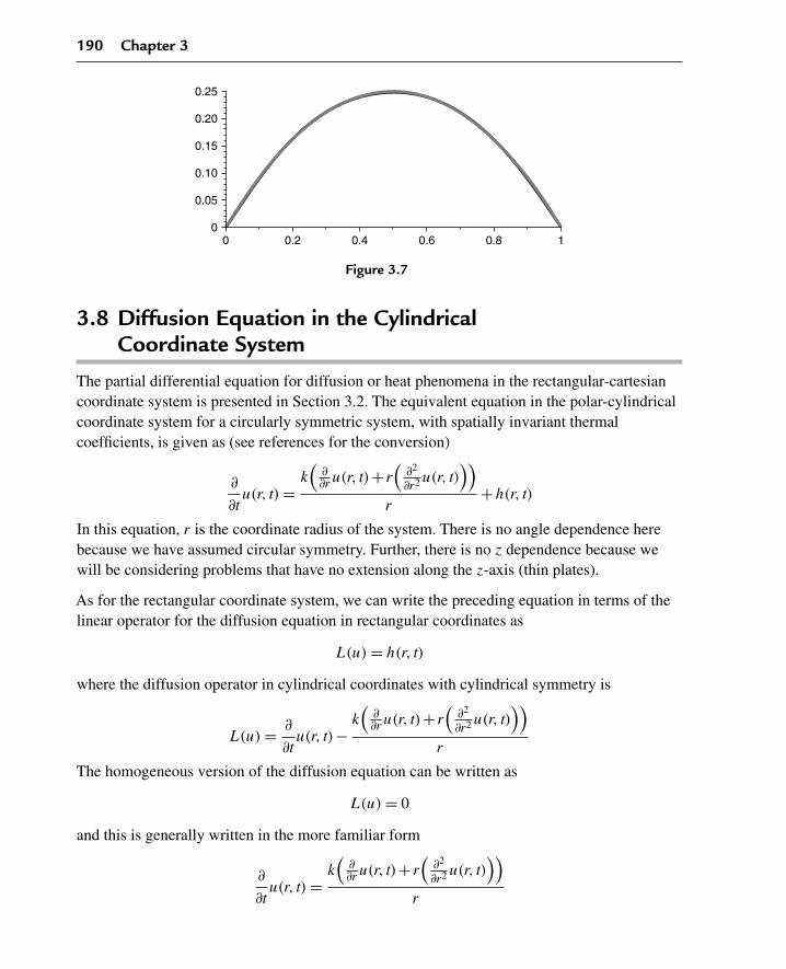
190 Chapter 3
00 0.2 0.4 0.6 0.8 1
0.05
0.10
0.15
0.20
0.25
Figure 3.7
3.8 Diffusion Equation in the CylindricalCoordinate System
The partial differential equation for diffusion or heat phenomena in the rectangular-cartesiancoordinate system is presented in Section 3.2. The equivalent equation in the polar-cylindricalcoordinate system for a circularly symmetric system, with spatially invariant thermalcoefficients, is given as (see references for the conversion)
∂
∂tu(r, t) =
k(
∂∂r u(r, t)+ r
(∂2
∂r2 u(r, t)))
r+h(r, t)
In this equation, r is the coordinate radius of the system. There is no angle dependence herebecause we have assumed circular symmetry. Further, there is no z dependence because wewill be considering problems that have no extension along the z-axis (thin plates).
As for the rectangular coordinate system, we can write the preceding equation in terms of thelinear operator for the diffusion equation in rectangular coordinates as
L(u) = h(r, t)
where the diffusion operator in cylindrical coordinates with cylindrical symmetry is
L(u) = ∂
∂tu(r, t)−
k(
∂∂r u(r, t)+ r
(∂2
∂r2 u(r, t)))
r
The homogeneous version of the diffusion equation can be written as
L(u) = 0
and this is generally written in the more familiar form
∂
∂tu(r, t) =
k(
∂∂r u(r, t)+ r
(∂2
∂r2 u(r, t)))
r

The Diffusion or Heat Partial Differential Equation 191
We seek solutions to this partial differential equation over the finite interval I = {r |a < r < b}subject to the nonregular homogeneous boundary conditions
|u(a, t)| < ∞and
κ1u(b, t)+κ2ur(b, t) = 0
and the initial condition
u(r,0) = f(r)
We now attempt to solve this partial differential equation using the method of separation ofvariables. We set
u(r, t) = R(r)T(t)
Substituting this into the preceding homogeneous partial differential equation, we get
R(r)
(d
dtT(t)
)=
k(
ddr
R(r)+ r(
d2
dr2 R(r)))
T(t)
r
Dividing both sides by the product solution yields
ddt
T(t)
kT(t)=
ddr
R(r)+ r(
d2
dr2 R(r))
R(r)r
Since the left-hand side of the preceding is an exclusive function of t and the right-hand side anexclusive function of r, and r and t are independent, then the only way we can ensure equalityfor all r and t is to set each side equal to a constant.
Doing so, we arrive at the following two ordinary differential equations in terms of theseparation constant λ2:
d
dtT(t)+kλ2T(t) = 0
and
d2
dr2R(r)+
ddr
R(r)
r+λ2R(r) = 0
The preceding differential equation in t is an ordinary first-order linear equation for which wealready have the solution from Chapter 1.
The second differential equation in the variable r is recognized from Section 1.10 as being anordinary Bessel differential equation of order zero. The solution of this equation is the Besselfunction of the first kind of order zero.

192 Chapter 3
It was noted in Section 2.6 that, for the Bessel differential equation, the point r = 0 is a regularsingular point of the differential equation. With appropriate boundary conditions over aninterval that includes the origin, we obtain a “nonregular” (singular) type Sturm-Liouvilleeigenvalue problem whose eigenfunctions form an orthogonal set.
Similar to regular Sturm-Liouville problems over finite intervals, there exists an infinitenumber of eigenvalues that can be indexed by the positive integers n. The indexed eigenvaluesand corresponding eigenfunctions are given, respectively, as
λn,Rn(r)
for n = 0,1,2,3, . . . .
The eigenfunctions form a “complete” set with respect to any piecewise smooth function overthe finite interval I = {r |a < r < b}. In Section 2.6, we examined the nature of theorthogonality of the Bessel functions, and we showed the eigenfunctions to be orthogonal withrespect to the weight function w(r) = r over a finite interval I. Further, the eigenfunctions canbe normalized and the corresponding statement of orthonormality reads
b∫a
Rn(r)Rm(r)r dr = δ(n,m)
where the term on the right is the familiar Kronecker delta function.
Using arguments similar to those for the regular Sturm-Liouville problem, we can write ourgeneral solution to the partial differential equation as a superposition of the products of thesolutions to each of the ordinary differential equations given earlier.
For the indexed values of λ, the solution to the preceding time-dependent equation is
Tn(t) = C(n)e−kλ2nt
where the coefficients C(n) are unknown arbitrary constants.
By the method of separation of variables, we arrive at an infinite number of indexed solutionsun(r, t) (n = 0,1,2,3, . . .) for the homogeneous diffusion partial differential equation, over afinite interval, given as
un(r, t) = Rn(r)C(n)e−kλ2nt
Because the differential operator is linear, then any superposition of solutions to thehomogeneous equation is also a solution. Thus, the general solution can be written as theinfinite sum
u(r, t) =∞∑
n=0
Rn(r)C(n)e−kλ2nt

The Diffusion or Heat Partial Differential Equation 193
We demonstrate the preceding concepts with an example diffusion problem in cylindricalcoordinates.
DEMONSTRATION: We seek the temperature distribution u(r, t) in a thin circularlysymmetric plate over the finite interval I = {r |0 < r < 1} whose lateral surface is insulated, sothere is no heat loss through the lateral surfaces. The periphery (edge) of the plate is at the fixedtemperature of zero. The initial temperature distribution f(r) is given below, and the diffusivityis k = 1/20.
SOLUTION: The homogeneous diffusion equation is
∂
∂tu(r, t) =
∂∂r u(r, t)+ r
(∂2
∂r2 u(r, t))
20r
The boundary conditions are type 1 at r = 1, and we require the solution to be finite at the origin
|u(0, t)| < ∞ and u(1, t) = 0
The initial condition is
u(r,0) = f(r)
From the method of separation of variables, we obtain the two ordinary differential equations:
d
dtT(t)+ λ2T(t)
20= 0
and
d2
dr2R(r)+
ddr
R(r)
r+λ2R(r) = 0
We first consider the spatial differential equation in r. This is a Bessel-type differentialequation of the first kind of order zero with boundary conditions
|R(0)| < ∞ and R(1) = 0
This same problem was considered in Example 2.6.2 in Chapter 2. The allowed eigenvalues arethe roots of the eigenvalue equation
J(0, λn) = 0
for n = 1,2,3,. . . , and the corresponding orthonormal eigenfunctions are
Rn(r) =√
2J(0, λnr)
J(1, λn)

194 Chapter 3
where J(0, λn) and J(1, λn) are the Bessel functions of the first kind of order zero and one,respectively. The corresponding statement of orthonormality with respect to the weightfunction w(r) = r over the interval I is
1∫0
2J(0, λnr)J(0, λmr)r
J(1, λn)J(1, λm)dr = δ(n,m)
We next consider the time-dependent differential equation. This is a first-order ordinarydifferential equation that we solved in Section 1.2. The solution for the allowed values of λ
given earlier reads
Tn(t) = C(n)e− λ2nt
20
Thus, the eigenfunction expansion for the solution to the problem reads
u(r, t) =∞∑
n=1
C(n)e− λ2nt
20√
2J(0, λnr)
J(1, λn)
The unknown coefficients C(n), for n = 1,2,3,. . . , are to be determined from the initialcondition function imposed on the problem.
3.9 Initial Conditions for the Diffusion Equation inCylindrical Coordinates
We now consider the initial conditions on the problem. If the initial condition temperaturedistribution is given as
u(r,0) = f(r)
then substitution of this into the following general solution
u(r, t) =∞∑
n=0
Rn(r)C(n)e−kλ2nt
at time t = 0 yields
f(r) =∞∑
n=0
Rn(r)C(n)
This equation is the Fourier-Bessel series expansion of the function f(r), and the coefficientsC(n) are the Fourier coefficients.

The Diffusion or Heat Partial Differential Equation 195
As we did before for the generalized Fourier series expansion of a piecewise smooth functionover the finite interval I, we can evaluate the coefficients C(n) by taking the inner product ofboth sides of the preceding equation with the orthonormalized eigenfunctions with respect tothe weight function w(r) = r. Assuming validity of the interchange between the summationand integration operations, we get
b∫a
f(r)Rm(r)r dr =∞∑
n=0
C(n)
⎛⎝ b∫
a
Rn(r)Rm(r)r dr
⎞⎠
Taking advantage of the statement of orthonormality, this equation reduces to
b∫a
f(r)Rm(r)r dr =∞∑
n=0
C(n)δ(n,m)
Due to the mathematical character of the Kronecker delta function, only one term (n = m) inthe sum survives, and we get
C(m) =b∫
a
f(r)Rm(r)r dr
Thus, we can write the final generalized solution to the diffusion equation in cylindricalcoordinates in one dimension, subject to the given homogeneous boundary conditions andinitial conditions, as
u(r, t) =∞∑
n=0
Rn(r)e−kλ2nt
⎛⎝ b∫
a
f(s)Rn(s)s ds
⎞⎠
Again, all of the preceding operations are based on the assumption that the infinite series isuniformly convergent and the formal interchange between the operator and the summation islegitimate. It can be shown that if the initial condition function f(r) is piecewise smooth and itsatisfies the same boundary conditions as the eigenfunctions, then the preceding series is,indeed, uniformly convergent.
DEMONSTRATION: We now provide a demonstration of these concepts for the exampleproblem given in Section 3.8 for the case where the initial temperature distribution is
f(r) = 1− r2
SOLUTION: The unknown Fourier coefficients are to be evaluated from the integral
C(n) =1∫
0
(1− r2)√
2J(0, λnr)r
J(1, λn)dr

196 Chapter 3
Evaluation of this integral yields
C(n) = 4√
2
λ3n
for n = 1,2,3, . . . . Thus, the final series solution to our problem reads
u(r, t) =∞∑
n=1
8e− λ2nt
20 J(0, λnr)
λ3nJ(1, λn)
The detailed development of the solution of this problem along with the graphics are given inone of the Maple worksheet examples given later.
3.10 Example Diffusion Problems in CylindricalCoordinates
We now consider several examples of partial differential equations for heat or diffusionphenomena under various homogeneous boundary conditions over finite intervals in thecylindrical coordinate system. We note that all the spatial ordinary differential equations in thecylindrical coordinate system are of the Bessel type and the solutions are Bessel functions ofthe first kind.
EXAMPLE 3.10.1: We seek the temperature distribution u(r, t) in a thin circularly symmetricplate over the interval I = {r |0 < r < 1} whose lateral surface is insulated. The periphery(edge) of the plate is at the fixed temperature of zero. The initial temperature distribution f(r)
is given following, and the diffusivity is k = 1/20.
SOLUTION: The homogeneous diffusion equation is
∂2
∂t2u(r, t) =
k(
∂∂r u(r, t)+ r
(∂2
∂r2 u(r, t)))
r
The boundary conditions are type 1 at r = 1, and we require a finite solution at r = 0.
|u(0, t)| < ∞ and u(1, t) = 0
The initial condition is
u(r,0) = 1− r2
Ordinary differential equations obtained from the method of separation of variables are
d
dtT(t)+kλ2T(t) = 0

The Diffusion or Heat Partial Differential Equation 197
and
d2
dr2R(r)+
ddr
R(r)
r+λ2R(r) = 0
Boundary conditions on the spatial equation are
|R(0)| < ∞ and R(1) = 0
Assignment of system parameters
> restart:with(plots):a:=0:b:=1:k:=1/20:
Allowed eigenvalues and orthonormal eigenfunctions are from Example 2.6.2. The eigenvaluesare the roots of the eigenvalue equation
> BesselJ(0,lambda[n]*b)=0;
BesselJ(0, λn) = 0 (3.65)
for n = 1,2,3, . . . .
Orthonormal eigenfunctions
> R[n](r):=simplify(BesselJ(0,lambda[n]*r)/sqrt(int(BesselJ(0,lambda[n]*r)ˆ2*r,r=a..b)));
Rn(r) := BesselJ(0, λnr)√
2√BesselJ(0, λn)2 +BesselJ(1, λn)2
(3.66)
Substitution of the eigenvalue equation simplifies the preceding equation
> R[n](r):=radsimp(subs(BesselJ(0,lambda[n])=0,R[n](r)));R[m](r):=subs(n=m,R[n](r)):
Rn(r) := BesselJ(0, λnr)√
2
BesselJ(1, λn)(3.67)
Statement of orthonormality with respect to the weight function w(r) = r
> w(r):=r:Int(R[n](r)*R[m](r)*w(r),r=a...b)=delta(n,m);
1∫0
2BesselJ(0, λnr)BesselJ(0, λmr)r
BesselJ(1, λn)BesselJ(1, λm)dr = δ(n,m) (3.68)
Time-dependent solution
> T[n](t):=C(n)*exp(−k*lambda[n]ˆ2*t);u[n](r,t):=T[n](t)*R[n](r):
Tn(t) := C(n)e− 120 λ2
nt (3.69)
198 Chapter 3
Generalized series terms
> u[n](r,t):=T[n](t)*R[n](r);
un(r, t) := C(n)e− 120 λ2
ntBesselJ(0, λnr)√
2
BesselJ(1, λn)(3.70)
Eigenfunction expansion
> u(r,t):=Sum(u[n](r,t),n=1..infinity);
u(r, t) :=∞∑
n=1
C(n)e− 120 λ2
ntBesselJ(0, λnr)√
2
BesselJ(1, λn)(3.71)
Evaluation of Fourier coefficients for the specific initial condition
> f(r):=1−rˆ2;
f(r) := 1− r2 (3.72)
> C(n):=Int(f(r)*R[n](r)*w(r),r=a..b);
C(n) :=1∫
0
(1− r2)BesselJ(0, λnr)√
2r
BesselJ(1, λn)dr (3.73)
Substitution of the eigenvalue equation simplifies the preceding equation
> C(n):=simplify(subs(BesselJ(0,lambda[n])=0,value(%)));u[n](r,t):=eval(T[n](t)*R[n](r)):
C(n) := 4√
2
λ3n
(3.74)
Generalized series terms
> u[n](r,t):=eval(T[n](t)*R[n](r));
un(r, t) := 8e− 120 λ2
ntBesselJ(0, λnr)
λ3nBesselJ(1, λn)
(3.75)
Series solution
> u(r,t):=Sum(u[n](r,t),n=1..infinity);
u(r, t) :=∞∑
n=1
8e− 120 λ2
ntBesselJ(0, λnr)
λ3nBesselJ(1, λn)
(3.76)

The Diffusion or Heat Partial Differential Equation 199
Evaluation of the eigenvalues from the roots of the eigenvalue equation yields
> BesselJ(0,lambda[n]*b)=0;
BesselJ(0, λn) = 0 (3.77)
> plot(BesselJ(0,v),v=0..20,thickness=10);
20.4
20.2
05 10
v
15 20
0.4
0.2
0.6
0.8
1.0
Figure 3.8
If we set v = λb, then the eigenvalues are found from the intersection points of the curve withthe v-axis shown in Figure 3.8. We evaluate a few of these eigenvalues using the Maple fsolvecommand:
> lambda[1]:=(1/b)*fsolve(BesselJ(0,v)=0,v=0..3);
λ1 := 2.404825558 (3.78)
> lambda[2]:=(1/b)*fsolve(BesselJ(0,v)=0,v=3..6);
λ2 := 5.520078110 (3.79)
> lambda[3]:=(1/b)*fsolve(BesselJ(0,v)=0,v=6..9);
λ3 := 8.653727913 (3.80)
First few terms in sum
> u(r,t):=eval(sum(u[n](r,t),n=1..3)):
ANIMATION
> animate(u(r,t),r=a..b,t=0..5,thickness=3);
The preceding animation command illustrates the spatial-time-dependent solution for u(r, t).The animation sequence shown in Figure 3.9 shows snapshots at times t = 0,1,2,3,4, and 5.
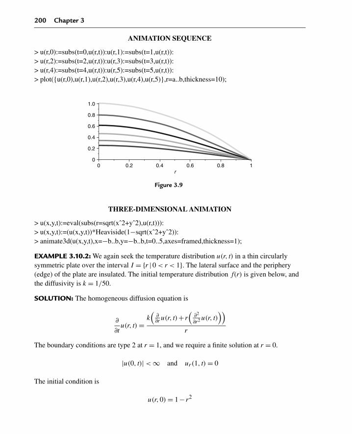
200 Chapter 3
ANIMATION SEQUENCE
> u(r,0):=subs(t=0,u(r,t)):u(r,1):=subs(t=1,u(r,t)):> u(r,2):=subs(t=2,u(r,t)):u(r,3):=subs(t=3,u(r,t)):> u(r,4):=subs(t=4,u(r,t)):u(r,5):=subs(t=5,u(r,t)):> plot({u(r,0),u(r,1),u(r,2),u(r,3),u(r,4),u(r,5)},r=a..b,thickness=10);
00 0.2 0.4 0.6
r0.8 1
0.2
0.4
0.6
0.8
1.0
Figure 3.9
THREE-DIMENSIONAL ANIMATION
> u(x,y,t):=eval(subs(r=sqrt(xˆ2+yˆ2),u(r,t))):> u(x,y,t):=(u(x,y,t))*Heaviside(1−sqrt(xˆ2+yˆ2)):> animate3d(u(x,y,t),x=−b..b,y=−b..b,t=0..5,axes=framed,thickness=1);
EXAMPLE 3.10.2: We again seek the temperature distribution u(r, t) in a thin circularlysymmetric plate over the interval I = {r |0 < r < 1}. The lateral surface and the periphery(edge) of the plate are insulated. The initial temperature distribution f(r) is given below, andthe diffusivity is k = 1/50.
SOLUTION: The homogeneous diffusion equation is
∂
∂tu(r, t) =
k(
∂∂r u(r, t)+ r
(∂2
∂r2 u(r, t)))
r
The boundary conditions are type 2 at r = 1, and we require a finite solution at r = 0.
|u(0, t)| < ∞ and ur(1, t) = 0
The initial condition is
u(r,0) = 1− r2

The Diffusion or Heat Partial Differential Equation 201
Ordinary differential equations obtained from the method of separation of variables are
d
dtT(t)+kλ2T(t) = 0
and
d2
dr2R(r)+
ddr
R(r)
r+λ2R(r) = 0
Boundary conditions on the spatial equation
|R(0)| < ∞ and Rr(1) = 0
Assignment of system parameters
> restart:with(plots):a:=0:b:=1:k:=1/50:
Allowed eigenvalues and orthonormal eigenfunctions are obtained from Example 2.6.3.
> lambda[0]:=0;
λ0 := 0 (3.81)
for n = 0.
Orthonormal eigenfunction
> R[0](r):=sqrt(2)/b;
R0(r) := √2 (3.82)
For n = 1,2,3, . . . , the eigenvalues are the roots of the eigenvalue equation
> subs(r=b,diff(BesselJ(0,lambda[n]*r),r))=0;
−BesselJ(1, λn)λn = 0 (3.83)
Orthonormal eigenfunctions
> R[n](r):=simplify(BesselJ(0,lambda[n]*r)/sqrt(int(BesselJ(0,lambda[n]*r)ˆ2*r,r=a..b)));
Rn(r) := BesselJ(0, λnr)√
2√BesselJ(0, λn)2 +BesselJ(1, λn)2
(3.84)
Substitution of the eigenvalue equation simplifies the preceding equation
> R[n](r):=radsimp(subs(BesselJ(1,lambda[n])=0,R[n](r)));R[m](r):=subs(n=m,R[n](r)):
Rn(r) := BesselJ(0, λnr)√
2
BesselJ(0, λn)(3.85)

202 Chapter 3
Statement of orthonormality with respect to the weight function w(r) = r
> w(r):=r:Int(R[n](r)*R[m](r)*w(r),r=a...b)=delta(n,m);
1∫0
2 BesselJ(0, λnr)BesselJ(0, λmr)r
BesselJ(0, λn)BesselJ(0, λm)dr = δ(n,m) (3.86)
Time-dependent solution for n = 1,2,3, . . . reads
> T[n](t):=C(n)*exp(−k*lambda[n]ˆ2*t);u[n](r,t):=T[n](t)*R[n](r);
Tn(t) := C(n)e− 150 λ2
nt (3.87)
Generalized series terms
> u[n](r,t):=T[n](t)*R[n](r);
un(r, t) := C(n)e− 150 λ2
ntBesselJ(0, λnr)√
2
BesselJ(0, λn)(3.88)
and for n = 0,
> T[0](t):=C(0);u[0](r,t):=T[0](t)*R[0](r):
T0(t) := C(0) (3.89)
Eigenfunction expansion
> u(r,t):=u[0](r,t)+Sum(u[n](r,t),n=1..infinity);
u(r, t) := C(0)√
2+∞∑
n=1
C(n)e− 150 λ2
ntBesselJ(0, λnr)√
2
BesselJ(0, λn)(3.90)
Evaluation of Fourier coefficients from the given specific initial condition
> f(r):=1−rˆ2;
f(r) := 1− r2 (3.91)
yields, for n = 0,
> C(0):=eval(Int(f(r)*R[0](r)*r,r=a..b));
C(0) :=1∫
0
(1− r2
)√2r dr (3.92)

The Diffusion or Heat Partial Differential Equation 203
> C(0):=value(%);u[0](r,t):=eval(T[0](t)*R[0](r)):
C(0) := 1
4
√2 (3.93)
and for n = 1,2,3, . . . ,
> C(n):=Int(f(r)*R[n](r)*r,r=a..b);
C(n) :=1∫
0
(1− r2
)BesselJ(0, λnr)
√2r
BesselJ(0, λn)dr (3.94)
Substitution of the eigenvalue equation simplifies the preceding equation
> C(n):=radsimp(subs(BesselJ(1,lambda[n]*b)=0,value(%)));
C(n) := −2√
2
λ2n
(3.95)
Generalized series terms
> u[n](r,t):=eval(T[n](t)*R[n](r));
un(r, t) := −4 e− 150 λ2
ntBesselJ(0, λnr)
λ2nBesselJ(0, λn)
(3.96)
Series solution
> u(r,t):=u[0](r,t)+Sum(u[n](r,t),n=1..infinity);
u(r, t) := 1
2+
∞∑n=1
(−4 e− 1
50 λ2ntBesselJ(0, λnr)
λ2nBesselJ(0, λn)
)(3.97)
Evaluation of the eigenvalues from the roots of the eigenvalue equation yields
> BesselJ(1,lambda[n]*b)=0;
BesselJ(1, λn) = 0 (3.98)
> plot(BesselJ(1,v),v=0..20,thickness=10);
If we set v = λb, then the eigenvalues are found from the intersection points of the curve withthe v-axis shown in Figure 3.10. We evaluate a few of these eigenvalues using the Maple fsolvecommand:
> lambda[1]:=(1/b)*fsolve(BesselJ(1,v)=0,v=1..4);
λ1 := 3.831705970 (3.99)

204 Chapter 3
20.2
20.3
20.1
05 10
v15 20
0.2
0.1
0.3
0.4
0.5
Figure 3.10
> lambda[2]:=(1/b)*fsolve(BesselJ(1,v)=0,v=4..8);
λ2 := 7.015586670 (3.100)
> lambda[3]:=(1/b)*fsolve(BesselJ(1,v)=0,v=8..12);
λ3 := 10.17346814 (3.101)
First few terms in the sum
> u(r,t):=u[0](r,t)+eval(sum(u[n](r,t),n=1..1)):
ANIMATION
> animate(u(r,t),r=a..b,t=0..5,thickness=3);
The preceding animation command illustrates the spatial-time-dependent solution for u(r, t).The animation sequence shown in Figure 3.11 shows snapshots at times t = 0,1,2,3,4, and 5.
ANIMATION SEQUENCE
> u(r,0):=subs(t=0,u(r,t)):u(r,1):=subs(t=1,u(r,t)):> u(r,2):=subs(t=2,u(r,t)):u(r,3):=subs(t=3,u(r,t)):> u(r,4):=subs(t=4,u(r,t)):u(r,5):=subs(t=5,u(r,t)):> plot({u(r,0),u(r,1),u(r,2),u(r,3),u(r,4),u(r,5)},r=a..b,thickness=10);
THREE-DIMENSIONAL ANIMATION
> u(x,y,t):=eval(subs(r=sqrt(xˆ2+yˆ2),u(r,t))):> u(x,y,t):=(u(x,y,t))*Heaviside(1−sqrt(xˆ2+yˆ2)):> animate3d(u(x,y,t),x=−b..b,y=−b..b,t=0..5,axes=framed,thickness=1);

The Diffusion or Heat Partial Differential Equation 205
0.3
0.0 0.2 0.4 0.6r
0.8 1
0.40.50.60.70.80.91.01.1
Figure 3.11
Chapter Summary
Nonhomogeneous one-dimensional diffusion equation in rectangular coordinates
∂
∂tu(x, t) = k
(∂2
∂x2u(x, t)
)+h(x, t)
Linear diffusion operator of one dimension in rectangular coordinates
L(u) = ∂
∂tu(x, t)−k
(∂2
∂x2u(x, t)
)
Method of separation of variables solution
u(x, t) = X(x)T(t)
Eigenfunction expansion solution for rectangular coordinates
u(x, t) =∞∑
n=0
Xn(x)C(n)e−kλnt
Initial condition Fourier coefficients for rectangular coordinates
C(n) =∫ b
af(x)Xn(x)dx
Nonhomogeneous one-dimensional diffusion equation in cylindrical coordinates
∂
∂tu(r, t) =
k(
∂∂r u(r, t)+ r
(∂2
∂r2 u(r, t)))
r+h(r, t)

206 Chapter 3
Linear diffusion operator of one dimension in cylindrical coordinates
L(u) = ∂
∂tu(r, t)−
k(
∂∂r u(r, t)+ r
(∂2
∂r2 u(r, t)))
r
Method of separation of variables solution
u(r, t) = R(r)T(t)
Eigenfunction expansion solution in cylindrical coordinates
u(r, t) =∞∑
n=0
Rn(r)C(n)e−kλ2nt
Initial condition Fourier coefficients for cylindrical coordinates
C(n) =∫ b
af(r)Rn(r)r dr
We have examined partial differential equations describing diffusion or heat diffusionphenomena in a single spatial dimension for both the rectangular and the cylindrical coordinatesystems. We examine these same partial differential equations in steady-state and higher-dimensional systems later.
Exercises
We now consider exercise problems dealing with diffusion or heat equations with homogeneousboundary conditions in both the rectangular and the cylindrical coordinate systems. Use themethod of separation of variables and eigenfunction expansions to evaluate the solutions.
3.1. Consider the temperature distribution in a thin rod over the interval I = {x |0 < x < 1}whose lateral surface is insulated. The homogeneous partial differential equation reads
∂
∂tu(x, t) = k
(∂2
∂x2u(x, t)
)
with k = 1/10, initial condition u(x,0) = f(x) given following, and boundaryconditions
u(0, t) = 0, u(1, t) = 0
that is, the left end of the rod is at the fixed temperature zero and the right end is at thefixed temperature zero. Evaluate the eigenvalues and corresponding orthonormalized

The Diffusion or Heat Partial Differential Equation 207
eigenfunctions, and write the general solution for each of these three initial conditionfunctions:
f1(x) = 1
f2(x) = x
f3(x) = x(1−x) (3.102)
Generate the animated solution for each case, and plot the animated sequence for0 < t < 5. In the animated sequence, take note of the adherence of the solution to theboundary conditions.
3.2. Use the three-step verification procedure in Exercise 3.1 for the case u(x,0) = f3(x).
3.3. Consider the temperature distribution in a thin rod over the interval I = {x |0 < x < 1}whose lateral surface is insulated. The homogeneous partial differential equation reads
∂
∂tu(x, t) = k
(∂2
∂x2u(x, t)
)
with k = 1/10, initial condition u(x,0) = f(x) given later, and boundary conditions
u(0, t) = 0, ux(1, t) = 0
that is, the left end of the rod is at the fixed temperature zero and the right end isinsulated. Evaluate the eigenvalues and corresponding orthonormalized eigenfunctions,and write the general solution for each of these three initial condition functions:
f1(x) = x2
f2(x) = x
f3(x) = x(
1− x
2
)Generate the animated solution for each case, and plot the animated sequence for0 < t < 5. In the animated sequence, take note of the adherence of the solution to theboundary conditions.
3.4. Use the three-step verification procedure in Exercise 3.3 for the case u(x,0) = f3(x).
3.5. Consider the temperature distribution in a thin rod over the interval I = {x |0 < x < 1}whose lateral surface is insulated. The homogeneous partial differential equation reads
∂
∂tu(x, t) = k
(∂2
∂x2u(x, t)
)

208 Chapter 3
with k = 1/10, initial condition u(x,0) = f(x) given later, and boundary conditions
ux(0, t) = 0, u(1, t) = 0
that is, the left end of the rod is insulated and the right end is at the fixed temperaturezero. Evaluate the eigenvalues and the corresponding orthonormalized eigenfunctions,and write the general solution for each of these three initial condition functions:
f1(x) = x
f2(x) = 1
f3(x) = 1−x2
Generate the animated solution for each case, and plot the animated sequence for0 < t < 5. In the animated sequence, take note of the adherence of the solution to theboundary conditions.
3.6. Use the three-step verification procedure in Exercise 3.5 for the case u(x,0) = f3(x).
3.7. Consider the temperature distribution in a thin rod over the interval I = {x |0 < x < 1}whose lateral surface is insulated. The homogeneous partial differential equation reads
∂
∂tu(x, t) = k
(∂2
∂x2u(x, t)
)
with k = 1/10, initial condition u(x,0) = f(x) given later, and boundary conditions
ux(0, t) = 0, ux(1, t) = 0
that is, the left end of the rod is insulated and the right end is insulated. Evaluate theeigenvalues and corresponding orthonormalized eigenfunctions, and write the generalsolution for each of these three initial condition functions:
f1(x) = x
f2(x) = 1−x2
f3(x) = x2(
1− 2x
3
)
Generate the animated solution for each case, and plot the animated sequence for0 < t < 5. In the animated sequence, take note of the adherence of the solution to theboundary conditions.
3.8. Use the three-step verification procedure in Exercise 3.7 for the case u(x,0) = f3(x).

The Diffusion or Heat Partial Differential Equation 209
3.9. Consider the temperature distribution in a thin rod over the interval I = {x |0 < x < 1}whose lateral surface is insulated. The homogeneous partial differential equation reads
∂
∂tu(x, t) = k
(∂2
∂x2u(x, t)
)
with k = 1/10, initial condition u(x,0) = f(x) given later, and boundary conditions
u(0, t) = 0, u(1, t)+ux(1, t) = 0
that is, the left end of the rod is at a fixed temperature zero, and the right end is losingheat by convection into a zero temperature surrounding. Evaluate the eigenvalues andcorresponding orthonormalized eigenfunctions, and write the general solution for eachof these three initial condition functions:
f1(x) = 1
f2(x) = x
f3(x) = x
(1− 2x
3
)
Generate the animated solution for each case, and plot the animated sequence for0 < t < 5. In the animated sequence, take note of the adherence of the solution to theboundary conditions.
3.10. Use the three-step verification procedure in Exercise 3.9 for the case u(x,0) = f3(x).
3.11. Consider the temperature distribution in a thin rod over the interval I = {x |0 < x < 1}whose lateral surface is insulated. The homogeneous partial differential equation reads
∂
∂tu(x, t) = k
(∂2
∂x2u(x, t)
)
with k = 1/10, initial condition u(x,0) = f(x) given later, and boundary conditions
u(0, t)−ux(0, t) = 0, u(1, t) = 0
that is, the left end of the rod is losing heat by convection into a zero temperaturesurrounding and the right end is at a fixed temperature zero. Evaluate the eigenvaluesand corresponding orthonormalized eigenfunctions, and write the general solution foreach of these three initial condition functions:
f1(x) = 1
f2(x) = 1−x
f3(x) = −2x2
3+ x
3+ 1
3
210 Chapter 3
Generate the animated solution for each case, and plot the animated sequence for0 < t < 5. In the animated sequence, take note of the adherence of the solution to theboundary conditions.
3.12. Use the three-step verification procedure in Exercise 3.11 for the case u(x,0) = f3(x).
3.13. Consider the temperature distribution in a thin rod over the interval I = {x |0 < x < 1}whose lateral surface is insulated. The homogeneous partial differential equation reads
∂
∂tu(x, t) = k
(∂2
∂x2u(x, t)
)
with k = 1/10, initial condition u(x,0) = f(x) given later, and boundary conditions
ux(0, t) = 0, u(1, t)+ux(1, t) = 0
that is, the left end of the rod is insulated and the right end is losing heat by convectioninto a zero temperature surrounding. Evaluate the eigenvalues and correspondingorthonormalized eigenfunctions, and write the general solution for each of these threeinitial condition functions:
f1(x) = x
f2(x) = 1
f3(x) = 1− x2
3
Generate the animated solution for each case, and plot the animated sequence for0 < t < 5. In the animated sequence, take note of the adherence of the solution to theboundary conditions.
3.14. Use the three-step verification procedure in Exercise 3.13 for the case u(x,0) = f3(x).
3.15. Consider the temperature distribution in a thin rod over the interval I = {x |0 < x < 1}whose lateral surface is insulated. The homogeneous partial differential equation reads
∂
∂tu(x, t) = k
(∂2
∂x2u(x, t)
)
with k = 1/10, initial condition u(x,0) = f(x) given later, and boundary conditions
u(0, t)−ux(0, t) = 0, ux(1, t) = 0
that is, the left end of the rod is losing heat by convection into a zero temperaturesurrounding and the right end is insulated. Evaluate the eigenvalues and corresponding

The Diffusion or Heat Partial Differential Equation 211
orthonormalized eigenfunctions, and write the general solution for each of these threeinitial condition functions:
f1(x) = x
f2(x) = 1
f3(x) = 1− (x−1)2
3
Generate the animated solution for each case, and plot the animated sequence for0 < t < 5. In the animated sequence, take note of the adherence of the solution to theboundary conditions.
3.16. Use the three-step verification procedure in Exercise 3.15 for the case u(x,0) = f3(x).
3.17. Consider the temperature distribution in a thin rod over the interval I = {x |0 < x < 1}whose lateral surface is not insulated. The rod is experiencing a heat loss proportionalto the difference between the rod temperature and the surrounding temperature at zerodegrees. The homogeneous partial differential equation reads
∂
∂tu(x, t) = k
(∂2
∂x2u(x, t)
)−βu(x, t)
with k = 1/10, β = 1/4, initial condition u(x,0) = f(x) given later, and boundaryconditions
u(0, t) = 0, u(1, t) = 0
that is, the left end of the rod is at the fixed temperature zero and the right end is at thefixed temperature zero. Evaluate the eigenvalues and corresponding orthonormalizedeigenfunctions, and write the general solution for each of these three initial conditionfunctions:
f1(x) = 1
f2(x) = x
f3(x) = x(1−x)
Generate the animated solution for each case, and plot the animated sequence for0 < t < 5. In the animated sequence, take note of the adherence of the solution to theboundary conditions.
3.18. Consider the temperature distribution in a thin rod over the interval I = {x |0 < x < 1}whose lateral surface is not insulated. The rod is experiencing a heat loss proportional

212 Chapter 3
to the difference between the rod temperature and the surrounding temperature at zerodegrees. The homogeneous partial differential equation reads
∂
∂tu(x, t) = k
(∂2
∂x2u(x, t)
)−βu(x, t)
with k = 1/10, β = 1/4, initial condition u(x,0) = f(x) given later, and boundaryconditions
ux(0, t) = 0, u(1, t) = 0
that is, the left end of the rod is insulated and the right end is at a fixed temperature zero.Evaluate the eigenvalues and corresponding orthonormalized eigenfunctions, and writethe general solution for each of these three initial condition functions:
f1(x) = x
f2(x) = 1
f3(x) = 1−x2
Generate the animated solution for each case, and plot the animated sequence for0 < t < 5. In the animated sequence, take note of the adherence of the solution to theboundary conditions.
3.19. Consider the temperature distribution in a thin rod over the interval I = {x |0 < x < 1}whose lateral surface is not insulated. The rod is experiencing a heat loss proportionalto the difference between the rod temperature and the surrounding temperature at zerodegrees. The homogeneous partial differential equation reads
∂
∂tu(x, t) = k
(∂2
∂x2u(x, t)
)−βu(x, t)
with k = 1/10, β = 1/4, initial condition u(x,0) = f(x) given later, and boundaryconditions
ux(0, t) = 0, u(1, t)+ux(1, t) = 0
that is, the left end of the rod is insulated and the right end is losing heat by convectioninto a zero temperature surrounding. Evaluate the eigenvalues and correspondingorthonormalized eigenfunctions, and write the general solution for each of these threeinitial condition functions:
f1(x) = x
f2(x) = 1
f3(x) = 1− x2
3

The Diffusion or Heat Partial Differential Equation 213
Generate the animated solution for each case, and plot the animated sequence for0 < t < 5. In the animated sequence, take note of the adherence of the solution to theboundary conditions.
3.20. Consider the temperature distribution in a thin circularly symmetric plate over theinterval I = {r |0 < r < 1}. The lateral surface of the plate is insulated. Thehomogeneous partial differential equation reads
∂
∂tu(r, t) =
k(
∂∂r u(r, t)+ r
(∂2
∂r2 u(r, t)))
r
with k = 1/10, initial condition u(r,0) = f(r) given later, and boundary conditions
|u(0, t)| < ∞, u(1, t) = 0
that is, the center of the plate has a finite temperature and the periphery is at a fixedtemperature zero. Evaluate the eigenvalues and corresponding orthonormalizedeigenfunctions, and write the general solution for each of these three initial conditionfunctions:
f1(r) = r2
f2(r) = 1
f3(r) = 1− r2
Generate the animated solution for each case, and plot the animated sequence for0 < t < 5. In the animated sequence, take note of the adherence of the solution to theboundary conditions.
3.21. Consider the temperature distribution in a thin circularly symmetric plate over theinterval I = {r |0 < r < 1}. The lateral surface of the plate is insulated. Thehomogeneous partial differential equation reads
∂
∂tu(r, t) =
k(
∂∂r u(r, t)+ r
(∂2
∂r2 u(r, t)))
r
with k = 1/10, initial condition u(r,0) = f(r) given later, and boundary conditions
|u(0, t)| < ∞, ur(1, t) = 0
214 Chapter 3
that is, the center of the plate has a finite temperature and the periphery is insulated.Evaluate the eigenvalues and corresponding orthonormalized eigenfunctions, and writethe general solution for each of these three initial condition functions:
f1(r) = r2
f2(r) = 1
f3(r) = r2 − r4
2
Generate the animated solution for each case, and plot the animated sequence for0 < t < 5. In the animated sequence, take note of the adherence of the solution to theboundary conditions.
3.22. Consider the temperature distribution in a thin circularly symmetric plate over theinterval I = {r |0 < r < 1}. The lateral surface of the plate is insulated. Thehomogeneous partial differential equation reads
∂
∂tu(r, t) =
k(
∂∂r u(r, t)+ r
(∂2
∂r2 u(r, t)))
r
with k = 1/10, initial condition u(r,0) = f(r) given later, and boundary conditions
|u(0, t)| < ∞, ur(1, t)+u(1, t) = 0
that is, the center of the plate has a finite temperature and the periphery is losing heat byconvection into a zero temperature surrounding. Evaluate the eigenvalues andcorresponding orthonormalized eigenfunctions, and write the general solution for eachof these three initial condition functions:
f1(r) = r2
f2(r) = 1
f3(r) = 1− r2
3
Generate the animated solution for each case, and plot the animated sequence for0 < t < 5. In the animated sequence, take note of the adherence of the solution to theboundary conditions.

The Diffusion or Heat Partial Differential Equation 215
Significance of Thermal Diffusivity
The coefficient k in the heat equation is called the “thermal diffusivity” of the medium underconsideration. This constant is equal to
k = K
cρ
where c is the specific heat of the medium, ρ is the mass density, and K is the thermalconductivity of the medium. In a uniform, isotropic medium, these terms are all constants. Byconvention, we say that heat is a diffusion process whereby heat flows from high-temperatureregions to low-temperature regions similar to how salt in a water solution diffuses fromhigh-concentration regions to low-concentration regions. The magnitude of the thermaldiffusivity k is an indication of the ability of the medium to conduct heat from one region toanother. Thus, large values of k provide for rapid transfers and small values of k provide forslow transfers of heat within the medium.
In the following, we investigate the significance of the change in magnitude of the diffusivity k
by noting its effect on the solution of a problem. In Exercises 3.23 through 3.28, multiply thediffusivity by the given factor, and develop the solution for the given initial condition functionf3(x). Develop the animated solution and take particular note of the change in the timedependence of the solution due to the increased magnitude of the diffusivity.
3.23. In Exercise 3.1, multiply the diffusivity k by a factor of 5 and solve.
3.24. In Exercise 3.5, multiply the diffusivity k by a factor of 10 and solve.
3.25. In Exercise 3.9, multiply the diffusivity k by a factor of 5 and solve.
3.26. In Exercise 3.17, multiply the diffusivity k by a factor of 10 and solve.
3.27. In Exercise 3.20, multiply the diffusivity k by a factor of 5 and solve.
3.28. In Exercise 3.22, multiply the diffusivity k by a factor of 10 and solve.

This page intentionally left blank
CHAPTER 4
The Wave Partial DifferentialEquation
4.1 Introduction
We begin by examining types of partial differential equations that exhibit wave phenomena.We see wave-type partial differential equations in many areas of engineering and physics,including acoustics, electromagnetic theory, quantum mechanics, and the study of thetransmission of longitudinal and transverse disturbances in solids and liquids.
Similar to the partial differential equations that are descriptive of heat and diffusionphenomena, the wave partial differential equations that we examine here are also linear in thatthe partial differential operator L obeys the definition characteristics of a linear operatordefined in Section 3.1.
4.2 One-Dimensional Wave Operator in RectangularCoordinates
Wave phenomena in one dimension can be described by the following partial differentialequation in the rectangular coordinate system:
∂2
∂t2u(x, t) = c2
(∂2
∂x2u(x, t)
)−γ
(∂
∂tu(x, t)
)+h(x, t)
In the preceding, u(x, t) denotes the spatial-time-dependent wave amplitude, c denotes thewave speed, γ denotes the damping coefficient of the medium, and h(x, t) denotes the presenceof any external applied forces acting on the system. If the medium is uniform, then all thepreceding coefficients are spatially invariant, and we can write them as constants. The wavespeed c is generally proportional to the square root of the quotient of the tension in the systemand the inertia of the system (see Exercises 4.19 through 4.25).
© 2009, 2003, 1999 Elsevier Inc. 217

218 Chapter 4
We can write the preceding nonhomogeneous equation in terms of the linear wave operator as
L(u) = h(x, t)
where the wave operator in rectangular coordinates is
L(u) = ∂2
∂t2u(x, t)− c2
(∂2
∂x2u(x, t)
)+γ
(∂
∂tu(x, t)
)
If h(x, t) = 0, then there are no external applied forces acting on the system, and the precedingnonhomogeneous partial differential equation reduces to the corresponding homogeneousequation
L(u) = 0
For the case of no source terms and no damping in the system, the wave equation can bewritten in the more familiar form
∂2
∂t2u(x, t) = c2
(∂2
∂x2u(x, t)
)
This partial differential equation for wave phenomena is characterized by the fact that it relatesthe second partial derivative with respect to the time variable with the second partial derivativewith respect to the spatial variable.
Similar to what we did for the diffusion equation, some motivation for the derivation of thewave equation can be provided in terms of some simple concepts from introductory calculus.Recall that the slope of a curve of a function is found from the first derivative, and theconcavity of the curve is found from the second derivative with respect to the spatial variable x.In addition, the speed or time rate of change of a function is given as the first derivative, and itsacceleration is given as the second derivative with respect to the time variable t.
We imagine the sideview profile of a taut string that is secured at both end points. We assumesmall-amplitude vibrations of the string so the tension can be assumed to be invariant withrespect to time and position along the string. At those points along the string where the profileis most bent, as indicated by large values of concavity, we expect the string to want to resistfurther bending and to provide a large return force. From Newton’s second law, large forcesprovide large accelerations; thus, at regions of large concavity, the string should experiencelarge return accelerations. For a string whose local profile is concave down, we expect anegative return acceleration, which forces the string back to its unstretched position. Thus, theacceleration of the local profile is proportional to the spatial concavity of the profile: the exactbehavior as described by the preceding partial differential equation.
A typical example wave problem follows. We consider the waves describing the longitudinalvibrations in a rigid bar over the finite interval I = {x |0 < x < 1}. The left end of the bar issecure, and the right end is attached to an elastic hinge. The wave speed is c, and the damping

The Wave Partial Differential Equation 219
term γ is very small. The initial displacement distribution is f(x), and the initial speeddistribution is g(x).
The partial differential equation that describes the wave distribution u(x, t) for longitudinalvibrations in the bar is
∂2
∂t2u(x, t) = c2
(∂2
∂x2u(x, t)
)−γ
(∂
∂tu(x, t)
)
Since the bar is secured at the left end and hinged at the right end, the boundary conditions areof type 1 at x = 0 and type 3 at x = 1.
u(0, t) = 0
and
ux(1, t)+u(1, t) = 0
The initial displacement condition on the bar is
u(x,0) = f(x)
and the initial speed distribution is
ut(x,0) = g(x)
We solve this particular problem later. For now, we develop generalized procedures for thesolution to this homogeneous partial differential equation over a finite domain withhomogeneous boundary conditions using the method of separation of variables.
4.3 Method of Separation of Variables for theWave Equation
The homogeneous wave equation for a uniform system in one dimension in rectangularcoordinates can be written as
∂2
∂t2u(x, t)− c2
(∂2
∂x2u(x, t)
)+γ
(∂
∂tu(x, t)
)= 0
This can be rewritten in the more familiar form as
∂2
∂t2u(x, t)+γ
(∂
∂tu(x, t)
)= c2
(∂2
∂x2u(x, t)
)
Generally, one seeks a solution to this problem over the finite one-dimensional domainI = {x |a < x < b}, subject to the regular homogeneous boundary conditions
κ1u(a, t)+κ2ux(a, t) = 0

220 Chapter 4
and
κ3u(b, t)+κ4ux(b, t) = 0
and the two initial conditions
u(x,0) = f(x)
and
ut(x,0) = g(x)
Here, f(x) denotes the initial displacement of the wave, and g(x) denotes the initial speed ofthe amplitude of the wave.
In the method of separation of variables, the character of the equation is such that we canassume a solution in the form of a product as follows:
u(x, t) = X(x)T(t)
As in the case of the diffusion equation, because the two independent variables in the partialdifferential equation are the spatial variable x and the time variable t, then the precedingassumed solution is written as a product of two functions; one is exclusively a function of x
and the other an exclusive function of t.
Substituting this assumed solution into the partial differential equation yields
X(x)
(d2
dt2T(t)
)+γX(x)
(d
dtT(t)
)= c2
(d2
dx2X(x)
)T(t)
Dividing both sides of the preceding equation by the product solution gives us
d2
dt2T(t)+γ
(ddt
T(t))
c2T(t)=
d2
dx2 X(x)
X(x)
Since the left-hand side of the preceding is an exclusive function of t and the right-hand side anexclusive function of x, and t and x are independent, then the only way the preceding can holdfor all values of t and x is to set each side equal to a constant. Doing so, we get the followingtwo ordinary differential equations in terms of the separation constant λ:
d2
dt2T(t)+γ
(d
dtT(t)
)+ c2λT(t) = 0
and
d2
dx2X(x)+λX(x) = 0

The Wave Partial Differential Equation 221
This differential equation in t is an ordinary second-order linear homogeneous differentialequation for which we already have the solution from Section 1.4. Similarly, the seconddifferential equation in x is also an ordinary second-order linear homogeneous differentialequation for which we already have the solution from Section 1.4. We easily recognize thisdifferential equation as being of the Sturm-Liouville type.
4.4 Sturm-Liouville Problem for the Wave Equation
The second differential equation in the spatial variable x in the last section must be solvedsubject to the homogeneous spatial boundary conditions over the finite interval. TheSturm-Liouville problem for the wave equation consists of the ordinary differential equation
d2
dx2X(x)+λX(x) = 0
along with the corresponding homogeneous boundary conditions
κ1X(a)+κ2Xx(a) = 0
and
κ3X(b)+κ4Xx(b) = 0
We see the preceding problem in the spatial variable x to be a regular Sturm-Liouvilleeigenvalue problem where the allowed values of λ are called the system “eigenvalues” and thecorresponding solutions are called the “eigenfunctions.” Note that the ordinary differentialequation is of the Euler type and the weight function w(x) = 1.
It can be shown that for regular Sturm-Liouville problems over finite domains, an infinitenumber of eigenvalues exist that can be indexed by the integers n. The indexed eigenvaluesand corresponding eigenfunctions are given, respectively, as
λn,Xn(x)
for n = 0,1,2,3, . . . .
The eigenfunctions form a “complete” set with respect to any piecewise smooth function overthe finite interval I = {x |a < x < b}. Further, the eigenfunctions can be normalized and thecorresponding statement of orthonormality reads
b∫a
Xn(x)Xm(x)dx = δ(n,m)
where the term on the right is the familiar Kronecker delta function defined in Section 2.2.

222 Chapter 4
We now consider the time-dependent differential equation, which reads
d2
dt2T(t)+γ
(d
dtT(t)
)+ c2λT(t) = 0
From Section 1.4 on second-order linear differential equations, the solution to the precedingtime-dependent differential equation in terms of the allowed eigenvalues is
Tn(t) = A(n)e−γ t2 cos
(√4λnc2 −γ2 t
2
)+B(n)e−γ t
2 sin
(√4λnc2 −γ2 t
2
)
The coefficients A(n) and B(n) are unknown arbitrary constants. Throughout most of ourexample problems, we make the assumption that the damping in the system is small—that is,
γ2 < 4λnc2
This assumption gives rise to time-dependent solutions that are oscillatory. The argument ofthe preceding sinusoidal sine and cosine expressions denotes ωn, which is the damped angularfrequency of oscillation of the n-th term in the system. The damped angular frequency ofoscillation of the n-th term or mode is
ωn =√
4λnc2 −γ2
2
Thus, by the method of separation of variables, we arrive at an infinite number of indexedsolutions un(x, t) (n = 0,1,2,3, . . .) for the homogeneous wave partial differential equation,over a finite interval, given as
un(x, t) = Xn(x)e−γ t2 (A(n) cos(ωnt)+B(n) sin(ωnt))
Because the differential operator is linear, any superposition of solutions to the homogeneousequation is also a solution to the problem. Thus, we can write the general solution to thehomogeneous partial differential equation as the infinite sum
u(x, t) =∞∑
n=0
Xn(x)e−γ t2 (A(n) cos(ωnt)+B(n) sin(ωnt))
This equation is the eigenfunction expansion form of the solution to the wave partial differentialequation. The terms of the preceding sum form the “basis vectors” of the solution space of thepartial differential equation. Thus, for the wave partial differential equation, there are aninfinite number of basis vectors in the solution space, and we say the dimension of the solutionspace is infinite. This compares dramatically with an ordinary differential equation where thedimension of the solution space is finite and equal to the order of the equation. We demonstratethe preceding concepts with the solution of an illustrative problem given earlier in Section 4.2.

The Wave Partial Differential Equation 223
DEMONSTRATION: We seek the wave distribution u(x, t) for the longitudinal vibrations ina rigid bar over the finite interval I = {x |0 < x < 1}. The left end of the bar is secure, and theright end is attached to an elastic hinge. The wave speed is c and the damping term γ is verysmall. The initial displacement distribution is f(x), and the initial speed distribution is g(x).
SOLUTION: The partial differential equation that describes the longitudinal vibrations in thebar is
∂2
∂t2u(x, t) = c2
(∂2
∂x2u(x, t)
)−γ
(∂
∂tu(x, t)
)
Since the bar is secured at the left end and hinged at the right end, the boundary conditions areof type 1 at x = 0 and type 3 at x = 1.
u(0, t) = 0
and
ux(1, t)+u(1, t) = 0
The initial conditions on the bar are
u(x,0) = f(x)
and
ut(x,0) = g(x)
From the method of separation of variables, we get the two ordinary differential equations
d2
dt2T(t)+γ
(d
dtT(t)
)+ c2λT(t) = 0
and
d2
dx2X(x)+λX(x) = 0
We consider the solution to the spatial equation first. Again, the reason for this is that thespatial differential equation and the spatial boundary conditions determine the systemeigenvalues, and these eigenvalues must be determined before we consider the solution to thetime-dependent differential equation. Here, we have an Euler-type differential equation with atype 1 condition at the left and a type 3 condition at the right—that is,
X(0) = 0
and
Xx(1)+X(1) = 0

224 Chapter 4
We previously solved this problem in Example 2.5.4 in Chapter 2. The allowed eigenvalues arethe roots of the eigenvalue equation
tan(√
λn
)= −√
λn
and the corresponding orthonormalized eigenfunctions are
Xn(x) =√
2 sin(√
λnx)
√cos
(√λn
)2 +1
for n = 1,2,3, . . . .
The statement of orthonormality for the spatial eigenfunctions, with respect to the weightfunction w(x) = 1, is
1∫0
2sin
(√λn x
)sin
(√λm x
)√
cos(√
λn
)2 +1√
cos(√
λm
)2 +1dx = δ(n,m)
for n,m = 1,2,3, . . . .
The corresponding solution for the time-dependent differential equation is
Tn(t) = e−γ t2 (A(n) cos(ωnt)+B(n) sin(ωnt))
for n = 1,2,3, . . . .
The final eigenfunction expansion solution to the problem is constructed from the superpositionof the products of the preceding spatial and time-dependent solutions, and this reads
u(x, t) =∞∑
n=1
e−γ t2 (A(n) cos(ωnt)+B(n) sin(ωnt))
√2 sin
(√λnx
)√
cos(√
λn
)2 +1
The unknown coefficients A(n) and B(n) are to be determined from the initial conditions givenin the problem.
4.5 Initial Conditions for the Wave Equation inRectangular Coordinates
We now consider the initial conditions on the problem. At time t = 0, we have the initialdisplacement
u(x,0) = f(x)

The Wave Partial Differential Equation 225
and the initial amplitude speed
ut(x,0) = g(x)
Substituting the first condition into the general solution
u(x, t) =∞∑
n=0
Xn(x)e−γ t2 (A(n) cos(ωnt)+B(n) sin(ωnt))
at time t = 0 yields
f(x) =∞∑
n=0
Xn(x)A(n)
Substituting the second condition into the time derivative of the general solution at time t = 0yields
g(x) =∞∑
n=0
Xn(x)
(ωnB(n)− A(n)γ
2
)
Recall that the eigenfunctions of the regular Sturm-Liouville problem form a complete set withrespect to piecewise smooth functions over the finite interval I = {x |a < x < b}. Thus, both ofthe preceding equations are the generalized Fourier series expansions of the functions f(x) andg(x), respectively, in terms of the spatial eigenfunctions of the system. The terms A(n) andB(n) are the corresponding Fourier coefficients. We now evaluate these coefficients.
As we did in Section 2.3 for the generalized Fourier series expansion, we take the inner productof both sides of the preceding equations, with respect to the weight function w(x) = 1.Operating on the first equation, we get
b∫a
f(x)Xm(x)dx =∞∑
n=0
A(n)
⎛⎝ b∫
a
Xm(x)Xn(x)dx
⎞⎠
From the statement of orthonormality, this reduces to
b∫a
f(x)Xm(x)dx =∞∑
n=0
A(n)δ(n,m)
From the definition of the Kronecker delta function, only one term (n = m) survives in thesum, and we are able to extract the value
A(m) =b∫
a
f(x)Xm(x)dx

226 Chapter 4
In a similar manner, operating on the second equation and taking the inner product of bothsides, we get
b∫a
g(x)Xm(x)dx =∞∑
n=0
(ωnB(n)− A(n)γ
2
)⎛⎝ b∫
a
Xm(x)Xn(x)dx
⎞⎠
Again, taking advantage of the statement of orthonormality, the preceding equation reduces to
b∫a
g(x)Xm(x)dx =∞∑
n=0
(ωnB(n)− A(n)γ
2
)δ(n,m)
Evaluating the sum (only the n = m term survives) and inserting the known value for A(m)
yields
B(m) =
∫ b
a
(f(x)γ
2+g(x)
)Xm(x)dx
ωm
Thus, we can write the final generalized solution to the wave equation in one dimension,subject to the earlier homogeneous boundary conditions and initial conditions, as
u(x, t) =∞∑
n=0
Xn(x)e− γ t
2
⎛⎜⎜⎜⎝(∫ b
a
f(x)Xn(x)dx
)cos(ωnt)+
(∫ b
a
(f(x)γ
2+g(x)
)Xn(x)dx
)sin(wnt)
ωn
⎞⎟⎟⎟⎠
All of the operations given are based on the assumption that the infinite series is uniformlyconvergent and the formal interchange between the operator and the summation is legitimate.It can be shown that if the functions f(x) and g(x) satisfy the same boundary conditions as theeigenfunctions, then both of the preceding series are uniformly convergent. We demonstratethe evaluation of the coefficients A(n) and B(n) for the illustrative problem in Section 4.4.
DEMONSTRATION: Consider the case where the wave speed c = 1/4 and the dampingfactor γ = 1/5. The initial displacement distribution is
f(x) = x− 2x2
3
and the initial speed distribution is
g(x) = x

The Wave Partial Differential Equation 227
SOLUTION: The calculated value of ωn is
ωn =√
25λn −4
20
To evaluate A(n) and B(n), we take the inner products of the initial condition functions f(x)
and g(x), over the interval I = {x |0 < x < 1}, with the corresponding eigenfunctions. Doingso, we get
A(n) =1∫
0
(−2x2
3 +x)√
2 sin(√
λnx)
√cos
(√λn
)2 +1dx
which evaluates to
A(n) = − 4√
2(cos
(√λn
)−1)
3λ
(32
)n
√cos
(√λn
)2 +1
and
B(n) =
∫ 1
0
(− x2
15 + 11x10
)√2 sin
(√λnx
)√
cos(√
λn
)2 +1dx
ωn
which evaluates to
B(n) = −8√
2(15 cos
(√λn
)λn + cos
(√λn
)−1)
3√
25λn −4λ
(32
)n
√cos
(√λn
)2 +1
for n = 1,2,3, . . . .
For λ > 0, the eigenvalues λn are determined from the roots of the eigenvalue equation
tan(√
λn
)= −√
λn (4.1)
Figure 4.1 shows curves of the two functions tan(v) and −v plotted on the same set of axes. Ifwe set v = √
λ, then the eigenvalues are the squares of the values of v at the intersection pointsof these curves.
The first three eigenvalues are
λ1 = 4.115858365
λ2 = 24.13934203
λ3 = 63.65910654

228 Chapter 4
10 20
220
215
210
25
05 15
Figure 4.1
Combining all of the preceding, the final series solution to the problem reads
u(x, t) =∞∑
n=1
2 sin(√
λn x)
e− t10
⎛⎜⎜⎜⎝−
4(cos
(√λn
)−1)
cos
(√25λn −4 t
20
)
3λ
(32
)n
(cos
(√λn
)2 +1)
−8(15 cos
(√λn
)λn + cos
(√λn
)−1)
sin
(√25λn −4 t
20
)
3√
25λn −4 λ
(32
)n
(cos
(√λn
)2 +1)
⎞⎟⎟⎟⎠
The detailed development of the solution of this problem and the graphics are given in one ofthe Maple worksheet examples.
4.6 Example Wave Equation Problems in RectangularCoordinates
We now consider several examples of partial differential equations for wave phenomena undervarious homogeneous boundary conditions over finite intervals in the rectangular coordinatesystem. We note that all of the spatial ordinary differential equations in the rectangularcoordinate system are of the Euler type; thus, the weight function w(x) = 1.
EXAMPLE 4.6.1: We seek the wave distribution u(x, t) for transverse waves on a taut string,over the finite interval I = {x |0 < x < 1}. The string is tied at both ends. It is vibrating in aviscous medium with small damping, and there are no external forces acting. The string has aninitial displacement distribution f(x) and an initial speed distribution g(x) given following.The wave speed is c = 1/4, and the damping factor is γ = 1/5.

The Wave Partial Differential Equation 229
SOLUTION: The homogeneous wave equation is
∂2
∂t2u(x, t) = c2
(∂2
∂x2u(x, t)
)−γ
(∂
∂tu(x, t)
)
The boundary conditions are type 1 at x = 0 and type 1 at x = 1
u(0, t) = 0 and u(1, t) = 0
The initial conditions are
u(x,0) = x(1−x) and ut(x,0) = x(1−x)
The ordinary differential equations from the method of separation of variables are
d2
dt2T(t)+γ
(d
dtT(t)
)+ c2λT(t) = 0
and
d2
dx2X(x)+λX(x) = 0 (4.2)
The boundary conditions on the spatial equation are
X(0) = 0 and X(1) = 0
Assignment of system parameters
> restart:with(plots):a:=0:b:=1:c:=1/4:unprotect(gamma):gamma:=1/5:
Allowed eigenvalues and orthonormal eigenfunctions are obtained from Example 2.5.1.
> lambda[n]:=(n*Pi/b)ˆ2;
λn := n2π2 (4.3)
for n = 1,2,3, . . . .
> X[n](x):=sqrt(2/b)*sin(n*Pi/b*x);X[m](x):=subs(n=m,X[n](x)):
Xn(x) := √2 sin(nπx) (4.4)
Statement of orthonormality with respect to the weight function w(x) = 1
> w(x):=1:Int(X[n](x)*X[m](x)*w(x),x=a...b)=delta(n,m);
1∫0
2 sin(nπx) sin(mπx)dx = δ(n,m) (4.5)

230 Chapter 4
Time-dependent solution
> T[n](t):=exp((−gamma/2)*t)*(A(n)*cos(omega[n]*t)+B(n)*sin(omega[n]*t));
Tn(t) := e− 110 t
(A(n) cos(ωnt)+B(n) sin(ωnt)) (4.6)
Generalized series terms
> u[n](x,t):=T[n](t)*X[n](x):
Eigenfunction expansion
> u(x,t):=Sum(u[n](x,t),n=1..infinity);
u(x, t) :=∞∑
n=1
e− 110 t
(A(n) cos(ωnt)+B(n) sin(ωnt))√
2 sin(nπx) (4.7)
> omega[n]:=sqrt(lambda[n]*cˆ2−gammaˆ2/4);
ωn := 1
20
√25n2π2 −4 (4.8)
From Section 4.5, the coefficients A(n) and B(n) are to be determined from the inner product ofthe eigenfunctions and the given initial condition functions u(x,0) = f(x) and ut(x,0) = g(x).
> f(x):=x*(1−x);
f(x) := x(1−x) (4.9)
> g(x):=x*(1−x);
g(x) := x(1−x) (4.10)
For n = 1,2,3, . . . ,
> A(n):=Int(f(x)*X[n](x)*w(x),x=a..b);A(n):=expand(value(%)):
A(n) :=1∫
0
x(1−x)√
2 sin(nπx)dx (4.11)
> A(n):=simplify(subs({sin(n*Pi)=0,cos(n*Pi)=(−1)ˆn},A(n)));
A(n) := −2√
2(−1+ (−1)n)
π3n3(4.12)

The Wave Partial Differential Equation 231
> B(n):=Int((f(x)*gamma/2+g(x))*X[n](x)*w(x), x=a..b)/omega[n];B(n):=expand(value(%)):
B(n) :=20
⎛⎝
∫ 1
0
11
10x(1−x)
√2 sin(nπx)dx
⎞⎠
√25n2π2 −4
(4.13)
> B(n):=radsimp(subs({sin(n*Pi)=0, cos(n*Pi)=(−1)ˆn},%));
B(n) := −44√
2(−1+ (−1)n)
π3n3√
25n2π2 −4(4.14)
> T[n](t):=exp((−gamma/2)*t)*(A(n)*cos(omega[n]*t)+B(n)*sin(omega[n]*t)):
Generalized series terms
> u[n](x,t):=eval(T[n](t)*X[n](x)):
Series solution
> u(x,t):=Sum(u[n](x,t),n=1..infinity);
u(x, t) :=∞∑
n=1
e− 110 t
⎛⎝−
2√
2(−1+ (−1)n) cos(
120
√25n2π2 −4 t
)π3n3
(4.15)
−44
√2(−1+ (−1)n) sin
(120
√25n2π2 −4 t
)π3n3
√25n2π2 −4
⎞⎠√
2 sin(nπx)
First few terms of sum
> u(x,t):=sum(u[n](x,t),n=1..3):
ANIMATION
> animate(u(x,t),x=a..b,t=0..20,thickness=3);
The preceding animation command illustrates the spatial-time-dependent solution for u(x, t).The following animation sequence in Figure 4.2 shows snapshots of the animation at timest = 0,1,2,3,4, and 5.
ANIMATION SEQUENCE
> u(x,0):=subs(t=0,u(x,t)):u(x,1):=subs(t=1,u(x,t)):> u(x,2):=subs(t=2,u(x,t)):u(x,3):=subs(t=3,u(x,t)):> u(x,4):=subs(t=4,u(x,t)):u(x,5):=subs(t=5,u(x,t)):> plot({u(x,0),u(x,1),u(x,2),u(x,3),u(x,4),u(x,5)},x=a..b,thickness=10);

232 Chapter 4
x0.2 0.4 0.6 0.8 1
20.2
20.1
0
0.1
0.2
0.3
0.4
Figure 4.2
EXAMPLE 4.6.2: We seek the wave distribution u(x, t) for longitudinal vibrations in a rigidbar over the finite interval I = {x |0 < x < 1}. The left end of the bar is secured, and the rightend is unsecured. The damping is very small, and the bar has an initial displacementdistribution f(x) and an initial speed distribution g(x) given as follows. The wave speed isc = 1/4, and the damping factor is γ = 1/5.
SOLUTION: The homogeneous wave equation is
∂2
∂t2u(x, t) = c2
(∂2
∂x2u(x, t)
)−γ
(∂
∂tu(x, t)
)
The boundary conditions are type 1 at x = 0 and type 2 at x = 1
u(0, t) = 0 and ux(1, t) = 0
The initial conditions are
u(x,0) = x(
1− x
2
)and ut(x,0) = x
(1− x
2
)The ordinary differential equations from the method of separation of variables are
d2
dt2T(t)+γ
(d
dtT(t)
)+ c2λT(t) = 0
and
d2
dx2X(x)+λX(x) = 0 (4.16)
The boundary conditions on the spatial equation are
X(0) = 0 and Xx(1) = 0

The Wave Partial Differential Equation 233
Assignment of system parameters
> restart:with(plots):a:=0:b:=1:c:=1/4:unprotect(gamma):gamma:=1/5:
Allowed eigenvalues and orthonormal eigenfunctions are obtained from Example 2.5.2.
> lambda[n]:=((2*n−1)*Pi/(2*b))ˆ2;
λn := 1
4(2n−1)2π2 (4.17)
for n = 1,2,3, . . . .
> X[n](x):=sqrt(2/b)*sin((2*n−1)*Pi/(2*b)*x);X[m](x):=subs(n=m,X[n](x)):
Xn(x) := √2 sin
(1
2(2n−1)πx
)(4.18)
Statement of orthonormality with respect to the weight function w(x) = 1
> w(x):=1:Int(X[n](x)*X[m](x)*w(x),x=a..b)=delta(n,m);
1∫0
2 sin
(1
2(2n−1)πx
)sin
(1
2(2m−1)πx
)dx = δ(n,m) (4.19)
Time-dependent solution
> T[n](t):=exp((−gamma/2)*t)*(A(n)*cos(omega[n]*t)+B(n)*sin(omega[n]*t));u[n](x,t):=T[n](t)*X[n](x):
Tn(t) := e− 110 t
(A(n) cos(ωnt)+B(n) sin(ωnt)) (4.20)
Generalized series terms
> u[n](x,t):=T[n](t)*X[n](x):
Eigenfunction expansion
> u(x,t):=Sum(u[n](x,t),n=1..infinity);
u(x, t) :=∞∑
n=1
e− 110 t
(A(n) cos(ωnt)+B(n) sin(ωnt))√
2 sin
(1
2(2n−1)πx
)(4.21)
> omega[n]:=sqrt(lambda[n]*cˆ2−gammaˆ2/4);
ωn := 1
40
√25(2n−1)2π2 −16 (4.22)
From Section 4.5, the coefficients A(n) and B(n) are to be determined from the inner productof the eigenfunctions and the initial condition functions u(x,0) = f(x) and ut(x,0) = g(x).

234 Chapter 4
> f(x):=x*(1−x/2);
f(x) := x
(1− 1
2x
)(4.23)
> g(x):=x*(1−x/2);
g(x) := x
(1− 1
2x
)(4.24)
For n = 1,2,3, . . . ,
> A(n):=Int(f(x)*X[n](x)*w(x),x=a..b);A(n):=(value(%)):
A(n) :=1∫
0
x
(1− 1
2x
)√2 sin
(1
2(2n−1)πx
)dx (4.25)
> A(n):=factor(subs({sin(n*Pi)=0,cos(n*Pi)=(−1)ˆn},A(n)));
A(n) := 8√
2
(2n−1)3π3(4.26)
> B(n):=Int((f(x)*gamma/2+g(x))*X[n](x)*w(x),x=a..b)/omega[n];B(n):=(value(%)):
B(n) :=40
(∫ 1
0
11
10x
(1− 1
2x
)√2 sin
(1
2(2n−1)πx
)dx
)√
25(2n−1)2π2 −16(4.27)
> B(n):=subs({sin(n*Pi)=0,cos(n*Pi)=(−1)ˆn},B(n));
B(n) := 352√
2
π3(8n3 −12n2 +6n−1)√
25(2n−1)2π2 −16(4.28)
Generalized series terms
> u[n](x,t):=eval(T[n](t)*X[n](x)):
Series solution
> u(x,t):=Sum(u[n](x,t),n=1..infinity);
u(x, t) :=∞∑
n=1
e− 110 t
⎛⎝8
√2 cos
(140
√25(2n−1)2π2 −16 t
)(2n−1)3π3
(4.29)
+352
√2 sin
(1
40
√25(2n−1)2π2 −16 t
)π3(8n3 −12n2 +6n−1)
√25(2n−1)2π2 −16
⎞⎠√
2 sin
(1
2(2n−1)πx
)

The Wave Partial Differential Equation 235
First few terms of sum
> u(x,t):=sum(u[n](x,t),n=1..3):
ANIMATION
> animate(u(x,t),x=a..b,t=0..20,thickness=3);
The preceding animation command illustrates the spatial-time-dependent solution for u(x, t).The following animation sequence in Figure 4.3 shows snapshots of the animation at timest = 0,1,2,3,4, and 5.
ANIMATION SEQUENCE
> u(x,0):=subs(t=0,u(x,t)):u(x,1):=subs(t=1,u(x,t)):> u(x,2):=subs(t=2,u(x,t)):u(x,3):=subs(t=3,u(x,t)):> u(x,4):=subs(t=4,u(x,t)):u(x,5):=subs(t=5,u(x,t)):> plot({u(x,0),u(x,1),u(x,2),u(x,3),u(x,4),u(x,5)},x=a..b,thickness=10);
x0 0.2 0.4 0.6 0.8 1
0
0.2
0.4
0.6
0.8
1.0
Figure 4.3
EXAMPLE 4.6.3: We again consider the waves describing the longitudinal vibrations in arigid bar over the finite interval I = {x |0 < x < 1} with both ends unsecured. The damping isvery small. The initial displacement distribution f(x) and the initial speed distribution g(x) aregiven following. The wave speed is c = 1/4, and the damping factor is γ = 1/5.
SOLUTION: The homogeneous wave equation is
∂2
∂t2u(x, t) = c2
(∂2
∂x2u(x, t)
)−γ
(∂
∂tu(x, t)
)
The boundary conditions are type 2 at x = 0 and type 2 at x = 1
ux(0, t) = 0 and ux(1, t) = 0

236 Chapter 4
The initial conditions are
u(x,0) = 4x3 −6x2 +1 and ut(x,0) = 0
The ordinary differential equations from the method of separation of variables are
d2
dt2T(t)+γ
(d
dtT(t)
)+ c2λT(t) = 0
and
d2
dx2X(x)+λX(x) = 0 (4.30)
The boundary conditions on the spatial equation are
Xx(0) = 0 and Xx(1) = 0
Assignment of system parameters
> restart:with(plots):a:=0:b:=1:c:=1/4:unprotect(gamma):gamma:=1/5:
Allowed eigenvalues and orthonormal eigenfunctions are obtained from Example 2.5.4.
For n = 0,
> lambda[0]:=0;
λ0 := 0 (4.31)
> X[0](x):=1/sqrt(b);
X0(x) := 1 (4.32)
For n = 1,2,3, . . . ,
> lambda[n]:=(n*Pi/b)ˆ2;
λn := n2π2 (4.33)
> X[n](x):=sqrt(2/b)*cos(n*Pi/b*x);X[m](x):=subs(n=m,X[n](x)):
Xn(x) := √2 cos(nπx) (4.34)
Statement of orthonormality with respect to the weight function w(x) = 1
> w(x):=1:Int(X[n](x)*X[m](x)*w(x),x=a..b)=delta(n,m);
1∫0
2 cos(nπx) cos(mπx)dx = δ(n,m) (4.35)

The Wave Partial Differential Equation 237
Time-dependent solution
> T[0](t):=A(0)+B(0)*exp(−gamma*t);
T0(t) := A(0)+B(0)e−15 t (4.36)
For n = 0,
> T[n](t):=exp((−gamma/2)*t)*(A(n)*cos(omega[n]*t)+B(n)*sin(omega[n]*t));
Tn(t) := e− 110 t
(A(n) cos(ωnt)+B(n) sin(ωnt)) (4.37)
For n = 1,2,3, . . . ,
Generalized series terms
> u[0](x,t):=T[0](t)*X[0](x):u[n](x,t):=T[n](t)*X[n](x):
Eigenfunction expansion
> u(x,t):=u[0](x,t)+Sum(u[n](x,t),n=1..infinity);
u(x, t) := A(0)+B(0)e−15 t +
∞∑n=1
e− 110 t
(A(n) cos(ωnt)+B(n) sin(ωnt))√
2 cos(nπx) (4.38)
> omega[n]:=sqrt(lambda[n]*cˆ2−gammaˆ2/4);
ωn := 1
20
√25n2π2 −4 (4.39)
From Section 4.5, the coefficients A(n) and B(n) are to be determined from the inner productof the eigenfunctions and the initial condition functions u(x,0) = f(x) and ut(x,0) = g(x).
> f(x):=4*xˆ3−6*xˆ2+1;
f(x) := 4x3 −6x2 +1 (4.40)
> g(x):=0;
g(x) := 0 (4.41)
For n = 0,
> A(0):=(Int((f(x)*gamma+g(x))/gamma*X[0](x)*w(x),x=a..b));
A(0) :=1∫
0
(4x3 −6x2 +1)dx (4.42)

238 Chapter 4
> A(0):=value(%);
A(0) := 0 (4.43)
> B(0):=Int((−1/gamma)*g(x)*X[0](x)*w(x),x=a..b);
B(0) :=1∫
0
0 dx (4.44)
> B(0):=value(%);
B(0) := 0 (4.45)
For n = 1,2,3, . . . ,
> A(n):=eval(Int(f(x)*X[n](x)*w(x),x=a..b));A(n):=expand(value(%)):
A(n) :=1∫
0
(4x3 −6x2 +1)√
2 cos(nπx)dx (4.46)
> A(n):=simplify(subs({sin(n*Pi)=0,cos(n*Pi)=(−1)ˆn},A(n)));
A(n) := −24√
2 (−1+ (−1)n)
n4π4(4.47)
> B(n):=eval(Int((f(x)*gamma/2+g(x))*X[n](x)*w(x),x=a..b)/omega[n]);B(n):=expand(value(%)):
B(n) :=20
(∫ 1
0
(2
5x3 − 3
5x2 + 1
10
)√2 cos(nπx)dx
)√
25n2π2 −4(4.48)
> B(n):=simplify(subs({sin(n*Pi)=0,cos(n*Pi)=(−1)ˆn},B(n)));
B(n) := −48√
2 (−1+ (−1)n)
n4π4√
25n2π2 −4(4.49)
Generalized series terms
> u[0](x,t):=eval(T[0](t)*X[0](x)):u[n](x,t):=eval(T[n](t)*X[n](x)):

The Wave Partial Differential Equation 239
Series solution
> u(x,t):=u[0](x,t)+Sum(u[n](x,t),n=1..infinity);
u(x, t) :=∞∑
n=1
e− 110 t
⎛⎝−
24√
2(−1+ (−1)n) cos(
120
√25n2π2 −4 t
)n4π4
(4.50)
−48
√2(−1+ (−1)n) sin
(1
20
√25n2π2 −4 t
)n4π4
√25n2π2 −4
⎞⎠√
2 cos(nπx)
First few terms of sum
> u(x,t):=u[0](x,t)+sum(u[n](x,t),n=1..3):
ANIMATION
> animate(u(x,t),x=a..b,t=0..20,thickness=3);
The preceding animation command illustrates the spatial-time-dependent solution for u(x, t).Of particular note is that since the bar is initially extended symmetrically and both ends of thebar are unsecured, the subsequent vibrations indicate a symmetric longitudinal oscillation ofthe bar about its center. The following animation sequence in Figure 4.4 shows snapshots of theanimation at times t = 0,1,2,3,4, and 5.
ANIMATION SEQUENCE
> u(x,0):=subs(t=0,u(x,t)):u(x,1):=subs(t=1,u(x,t)):> u(x,2):=subs(t=2,u(x,t)):u(x,3):=subs(t=3,u(x,t)):> u(x,4):=subs(t=4,u(x,t)):u(x,5):=subs(t=5,u(x,t)):> plot({u(x,0),u(x,1),u(x,2),u(x,3),u(x,4),u(x,5)},x=a..b,thickness=10);
x0.2
20.820.620.420.2
00.20.40.60.8
0.4 0.6 0.8 1
Figure 4.4
EXAMPLE 4.6.4: We seek the wave distribution u(x, t) for longitudinal vibrations in a rigidbar over the finite interval I = {x |0 < x < 1}. The left end of the bar is secure, and the right
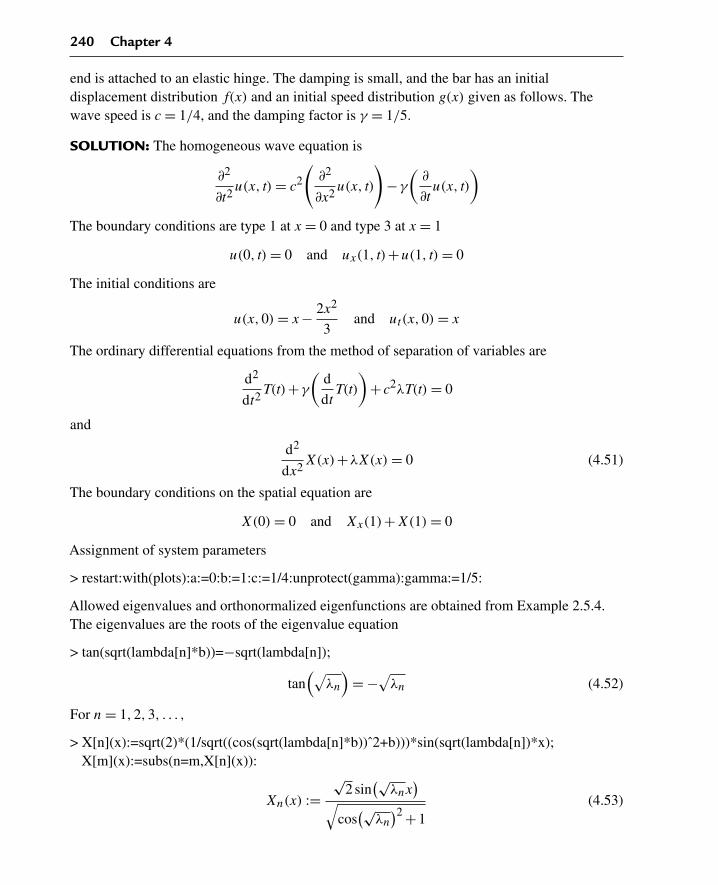
240 Chapter 4
end is attached to an elastic hinge. The damping is small, and the bar has an initialdisplacement distribution f(x) and an initial speed distribution g(x) given as follows. Thewave speed is c = 1/4, and the damping factor is γ = 1/5.
SOLUTION: The homogeneous wave equation is
∂2
∂t2u(x, t) = c2
(∂2
∂x2u(x, t)
)−γ
(∂
∂tu(x, t)
)
The boundary conditions are type 1 at x = 0 and type 3 at x = 1
u(0, t) = 0 and ux(1, t)+u(1, t) = 0
The initial conditions are
u(x,0) = x− 2x2
3and ut(x,0) = x
The ordinary differential equations from the method of separation of variables are
d2
dt2T(t)+γ
(d
dtT(t)
)+ c2λT(t) = 0
and
d2
dx2X(x)+λX(x) = 0 (4.51)
The boundary conditions on the spatial equation are
X(0) = 0 and Xx(1)+X(1) = 0
Assignment of system parameters
> restart:with(plots):a:=0:b:=1:c:=1/4:unprotect(gamma):gamma:=1/5:
Allowed eigenvalues and orthonormalized eigenfunctions are obtained from Example 2.5.4.The eigenvalues are the roots of the eigenvalue equation
> tan(sqrt(lambda[n]*b))=−sqrt(lambda[n]);
tan(√
λn
)= −√
λn (4.52)
For n = 1,2,3, . . . ,
> X[n](x):=sqrt(2)*(1/sqrt((cos(sqrt(lambda[n]*b))ˆ2+b)))*sin(sqrt(lambda[n])*x);X[m](x):=subs(n=m,X[n](x)):
Xn(x) :=√
2 sin(√
λnx)
√cos
(√λn
)2 +1(4.53)

The Wave Partial Differential Equation 241
Statement of orthonormality with respect to the weight function w(x) = 1
> w(x):=1:Int(X[n](x)*X[m](x)*w(x),x=a..b)=delta(n,m);
1∫0
2 sin(√
λnx)
sin(√
λmx)
√cos
(√λn
)2 +1√
cos(√
λm
)2 +1dx = δ(n,m) (4.54)
Time-dependent solution
> T[n](t):=exp((−gamma/2)*t)*(A(n)*cos(omega[n]*t)+B(n)*sin(omega[n]*t));
Tn(t) := e− 110 t
(A(n) cos(ωnt)+B(n) sin(ωnt)) (4.55)
Generalized series terms
> u[n](x,t):=T[n](t)*X[n](x):
Eigenfunction expansion
> u(x,t):=Sum(u[n](x,t),n=1..infinity);
u(x, t) :=∞∑
n=1
e− 110 t
(A(n) cos(ωnt)+B(n) sin(ωnt))√
2 sin(√
λnx)
√cos
(√λn
)2 +1(4.56)
> omega[n]:=sqrt(lambda[n]*cˆ2−gammaˆ2/4);
ωn := 1
20
√25λn −4 (4.57)
From Section 4.5, the coefficients A(n) and B(n) are to be determined from the innerproduct of the eigenfunctions and the initial condition functions u(x,0) = f(x) andut(x,0) = g(x).
> f(x):=x−2/3*xˆ2;
f(x) := x− 2
3x2 (4.58)
> g(x):=x;
g(x) := x (4.59)
For n = 1,2,3, . . . ,
> A(n):=eval(Int(f(x)*X[n](x)*w(x),x=a..b));A(n):=expand(value(%)):
A(n) :=1∫
0
(x− 2
3x2)√
2 sin(√
λnx)
√cos
(√λn
)2 +1dx (4.60)

242 Chapter 4
Substitution of the eigenvalue equation simplifies the preceding equation
> A(n):=simplify(subs(sin(sqrt(lambda[n])*b)=−sqrt(lambda[n])*cos(sqrt(lambda[n])*b),A(n)));
A(n) := −4
3
√2(−1+ cos
(√λn
))λ
(3/2)n
√cos
(√λn
)2 +1(4.61)
> B(n):=eval(Int((f(x)*gamma/2+g(x))*X[n](x)*w(x),x=a..b)/omega[n]);B(n):=expand(value(%)):
B(n) :=20
⎛⎜⎝∫ 1
0
(1110x− 1
15x2)√
2 sin(√
λnx)
√cos
(√λn
)2 +1dx
⎞⎟⎠
√25λn −4
(4.62)
Substitution of the eigenvalue equation simplifies this equation
> B(n):=simplify(subs(sin(sqrt(lambda[n])*b)=−sqrt(lambda[n])*cos(sqrt(lambda[n])*b),B(n)));
B(n) := −8
3
√2(−1+15 cos
(√λn
)λn + cos
(√λn
))λ
(3/2)n
√cos
(√λn
)2 +1√
25λn −4(4.63)
Generalized series terms
> u[n](x,t):=eval(T[n](t)*X[n](x)):
Series solution
> u(x,t):=Sum(u[n](x,t),n=1..infinity);
u(x, t) :=∞∑
n=1
1√cos
(√λn
)2 +1
⎛⎜⎝e− 1
10 t
⎛⎜⎝−4
3
√2(−1+ cos
(√λn
))cos
(120
√25λn −4 t
)λ
(3/2)n
√cos
(√λn
)2 +1
(4.64)
− 8
3
√2(−1+15 cos
(√λn
)λn + cos
(√λn
))sin
(120
√25λn −4 t
)λ
(3/2)n
√cos
(√λn
)2 +1√
25λn −4
⎞⎟⎠√
2 sin(√
λnx)⎞⎟⎠
Evaluation of the eigenvalues from the roots of the eigenvalue equation yields
> tan(sqrt(lambda[n])*b)=−sqrt(lambda[n]);
tan(√
λn
)= −√
λn (4.65)

The Wave Partial Differential Equation 243
> plot({tan(v),−v},v=0..20,y=−20..0,thickness=10);
10v
20
220
215
210
25
05 15
y
Figure 4.5
If we set v = √λb, then the eigenvalues are determined from the squares of the values of v at
the intersection points of the curves in Figure 4.5. Evaluation of the first few eigenvalues usingthe Maple fsolve command yields:
> lambda[1]:=(1/bˆ2)*(fsolve((tan(v)+v),v=1..3)ˆ2);
λ1 := 4.115858365 (4.66)
> lambda[2]:=(1/bˆ2)*(fsolve((tan(v)+v),v=3..6)ˆ2);
λ2 := 24.13934203 (4.67)
> lambda[3]:=(l/bˆ2)*(fsolve((tan(v)+v),v=6..9)ˆ2);
λ3 := 63.65910654 (4.68)
First few terms of sum
> u(x,t):=eval(sum(u[n](x,t),n=1..3)):
ANIMATION
> animate(u(x,t),x=a..b,t=0..20,thickness=3);
The preceding animation command illustrates the spatial-time-dependent solution for u(x, t).The following animation sequence in Figure 4.6 shows snapshots of the animation at timest = 0,1,2,3,4, and 5.
ANIMATION SEQUENCE
> u(x,0):=subs(t=0,u(x,t)):u(x,1):=subs(t=1,u(x,t)):> u(x,2):=subs(t=2,u(x,t)):u(x,3):=subs(t=3,u(x,t)):

244 Chapter 4
> u(x,4):=subs(t=4,u(x,t)):u(x,5):=subs(t=5,u(x,t)):> plot({u(x,0),u(x,1),u(x,2),u(x,3),u(x,4),u(x,5)},x=a..b,thickness=10);
x0 0.2 0.4 0.6 0.8 1
0
0.2
0.4
0.6
0.8
1
1.2
Figure 4.6
4.7 Wave Equation in the Cylindrical Coordinate System
The partial differential equation for wave phenomena in the cylindrical coordinate system fora circularly symmetric system is given below. Here, u(r, t) is the spatial-time-dependentsolution
∂2
∂t2u(r, t) =
c2(
∂∂r u(r, t)+ r
(∂2
∂r2 u(r, t)))
r−γ
(∂
∂tu(r, t)
)+h(r, t)
and r is the coordinate radius of the system. See the references for the equivalency of thewave equation from the rectangular cartesian system to the cylindrical coordinate system.There is no angle dependence here because we have assumed circular symmetry, and there isno z dependence because we will be considering regions with no extension along the z-axis.
As for the rectangular coordinate system, we can write the preceding in terms of the linearoperator for the wave equation in cylindrical coordinates as
L(u) = h(r, t)
where the wave operator in cylindrical coordinates reads as
L(u) = ∂2
∂t2u(r, t)−
c2(
∂∂r u(r, t)+ r
(∂2
∂r2 u(r, t)))
r+γ
(∂
∂tu(r, t)
)
We now consider the homogeneous version of the partial differential equation:
∂2
∂t2u(r, t)+γ
(∂∂t u(r, t)
)=
c2(
∂∂r u(r, t)+ r
(∂2
∂r2 u(r, t)))
r

The Wave Partial Differential Equation 245
We seek solutions to this partial differential equation over the finite interval I = {r |a < r < b}subject to the nonregular homogeneous boundary conditions
|u(a, t)| < ∞and
κ1u(b, t)+κ2ur(b, t) = 0
with the initial conditions
u(r,0) = f(r)
and
ut(r,0) = g(r)
Similar to the procedure for rectangular coordinates, we solve the partial differential equationusing the method of separation of variables. We set
u(r, t) = R(r)T(t)
Substituting this into the preceding homogeneous partial differential equation yields
R(r)
(d2
dt2T(t)+γ
(d
dtT(t)
))=
c2T(t)(
ddr
R(r)+ r(
d2
dr2 R(r)))
r
Dividing both sides by the product solution, we get
d2
dt2T(t)+γ
(ddt
T(t))
c2T(t)=
ddr
R(r)+ r(
d2
dr2 R(r))
R(r)r
Because the left-hand side of this equation is an exclusive function of t and the right-hand sidean exclusive function of r, and t and r are independent, then the only way we can ensureequality of the preceding for all r and t is to set each side equal to a constant.
Doing so, we arrive at the following two ordinary differential equations in terms of theseparation constant λ2:
d2
dt2T(t)+γ
(∂
∂tT(r, t)
)+λ2c2T(t) = 0
and
d2
dr2R(r)+
ddr
R(r)
r+λ2R(r) = 0
The preceding differential equation in t is an ordinary second-order linear differential equationfor which we already have the solution from Chapter 1.

246 Chapter 4
The second differential equation in the variable r is recognized from Section 1.11 as being anordinary Bessel differential equation. The solution of this equation is the Bessel function of thefirst kind of order zero.
We noted in Section 2.6 that, for the Bessel differential equation, the point r = 0 is a regularsingular point of the differential equation. With appropriate boundary conditions over aninterval that includes the origin, we arrive at a “nonregular” (singular) type Sturm-Liouvilleeigenvalue problem whose eigenfunctions form an orthogonal set.
Similar to regular Sturm-Liouville problems over finite intervals, an infinite number ofeigenvalues exist that can be indexed by the positive integers n. The indexed eigenvalues andcorresponding eigenfunctions are given, respectively, as
λn,Rn(r)
for n = 0,1,2,3, . . . .
The eigenfunctions form a “complete” set with respect to any piecewise smooth function overthe finite interval I = {r |a < r < b}. In Section 2.6, we examined the nature of theorthogonality of the Bessel functions, and we showed the eigenfunctions to be orthogonal withrespect to the weight function w(r) = r over the finite interval I. Further, the eigenfunctionscan be normalized, and the corresponding statement of orthonormality reads
b∫a
Rn(r)Rm(r)r dr = δ(n,m)
where the term on the right is the familiar Kronecker delta function.
Using arguments similar to that used for the regular Sturm-Liouville problem, we can writeour general solution to the partial differential equation as the superposition of the products ofthe solutions to each of the ordinary differential equations given earlier.
We now consider the time-dependent differential equation, which reads
d2
dt2T(t)+γ
(∂
∂tT(r, t)
)+λ2c2T(t) = 0
For the indexed values of λ, the solution to this equation is
Tn(t) = e−γt2 (A(n) cos(ωnt)+B(n) sin(ωnt))
where the n-th term damped angular frequency ωn is given in terms of the indexed λn as
ωn =√
4λ2nc2 −γ2
2

The Wave Partial Differential Equation 247
for n = 0,1,2,3, . . . . In the preceding equation, the coefficients A(n) and B(n) are unknownarbitrary constants and we have assumed small damping in the system—that is,
γ2 < 4λ2nc2
Thus, by the method of separation of variables, we arrive at an infinite number of indexedsolutions un(r, t) (n = 0,1,2,3, . . .) for the homogeneous wave partial differential equation,over a finite interval, given as
un(r, t) = Rn(r)e−γ t2 (A(n) cos(ωnt)+B(n) sin(ωnt))
Because the differential operator is linear, then any superposition of solutions to thehomogeneous equation is also a solution to the problem. Thus, we can write the generalsolution to the homogeneous partial differential equation as the infinite sum
u(r, t) =∞∑
n=0
Rn(r)e−γ t2 (A(n) cos(ωnt)+B(n) sin(ωnt))
We demonstrate the preceding concepts with an example wave problem in cylindricalcoordinates.
DEMONSTRATION: We seek the wave distribution u(r, t) for transverse vibrations in athin circularly symmetric membrane over the interval I = {r |0 < r < 1}, which is secureat the periphery. The membrane vibrates in a medium with a small amount of damping.The membrane has an initial displacement distribution f(r) and an initial speed distributiong(r) given as follows. The wave speed is c = 1/5, and the damping factor is γ = 2/5.
SOLUTION: The homogeneous wave equation is
∂2
∂t2u(r, t)+
2(
∂∂t u(r, t)
)5
=∂∂r u(r, t)+ r
(∂2
∂r2 u(r, t))
25r
The boundary conditions are type 1 at r = 1, and we require a finite solution at the origin
|u(0, t)| < ∞ and u(1, t) = 0
The initial conditions are
u(r,0) = f(r) and ut(r,0) = g(r)
From the method of separation of variables, the ordinary differential equations are
d2
dt2T(t)+
2(
ddt
T(t))
5+ λ2T(t)
25= 0

248 Chapter 4
and
d2
dr2R(r)+
ddr
R(r)
r+λ2R(r) = 0 (4.69)
We first consider the spatial differential equation in r. This is a Bessel-type differentialequation of the first kind of order zero with boundary conditions
|R(0)| < ∞ and R(1) = 0
This same problem was considered in Example 2.6.2 in Chapter 2. The allowed eigenvalues arethe roots of the eigenvalue equation
J(0, λn) = 0
and the corresponding orthonormal eigenfunctions are
Rn(r) =√
2J(0, λnr)
J(1, λn)
for n = 1,2,3, . . . . The functions J(0, λnr) and J(1, λnr) are Bessel functions of the first kindof order zero and one, respectively.
The corresponding statement of orthonormality with respect to the weight function w(r) = r
over the interval I is
1∫0
2J(0, λnr)J(0, λmr)r
J(1, λn)J(1, λm)dr = δ(n,m)
for n = 1,2,3, . . . , and m = 1,2,3, . . . .
We next consider the time-dependent differential equation. This is a second-order differentialequation that we solved in Section 1.4. The solution, for the allowed values of λ givenearlier, reads
Tn(t) = e− t5 (A(n) cos(ωnt)+B(n) sin(ωnt))
where
ωn =√
λ2n −1
5
Thus, the eigenfunction expansion solution to the problem reads
u(r, t) =∞∑
n=1
e− t5 (A(n) cos(ωnt)+B(n) sin(ωnt))
√2J(0, λnr)
J(1, λn)
The unknown coefficients A(n) and B(n) are to be determined from the initial conditionsimposed on the problem.

The Wave Partial Differential Equation 249
4.8 Initial Conditions for the Wave Equation inCylindrical Coordinates
We now consider the initial conditions on the problem. At time t = 0 we have the initialdisplacement
u(r,0) = f(r)
and the initial amplitude speed
ut(r,0) = g(r)
Substituting the first condition into the general solution
u(r, t) =∞∑
n=0
Rn(r)e−γt2 (A(n) cos(ωnt)+B(n) sin(ωnt))
at time t = 0 yields
f(r) =∞∑
n=0
Rn(r)A(n)
Substituting the second condition into the time derivative of the preceding at time t = 0 yields
g(r) =∞∑
n=0
Rn(r)
(B(n)ωn − A(n)γ
2
)
Because the eigenfunctions of this nonregular Sturm-Liouville problem form a complete setwith respect to piecewise smooth functions over the finite interval I = {r |a < r < b}, thenboth of the preceding equations are the generalized Fourier series expansions of the functionsf(r) and g(r), respectively, in terms of the spatial eigenfunctions of the system. We nowevaluate the coefficients A(n) and B(n).
As we did in Section 2.3 for the generalized Fourier series expansion, we take the innerproduct of both sides of the preceding equations, with respect to the weight function w(r) = r.Operating on the first equation and using the statement of orthonormality, we get
b∫a
f(r)Rm(r)r dr =∞∑
n=0
A(n)δ(n,m)
From the mathematical character of the Kronecker delta function, only one term (n = m)survives in the preceding sum, and we are able to extract the value
A(m) =b∫
a
f(r)Rm(r)r dr
250 Chapter 4
In a similar manner, operating on the second equation and taking the inner product of bothsides and using the statement of orthonormality, we get
b∫a
g(r)Rm(r)r dr =∞∑
n=0
(B(n)ωn − A(n)γ
2
)δ(n,m)
Evaluating the sum (only the n = m term survives) and inserting the preceding known valuefor A(m) yields
B(m) =
∫ b
a
(f(r)γ
2+g(r)
)Rm(r)r dr
ωm
Thus, we can write the final generalized solution to the wave equation in one dimension,subject to the preceding homogeneous boundary and initial conditions, as
u(r, t) =∞∑
n=0
Rn(r)e− γt
2
⎛⎜⎜⎜⎜⎜⎜⎜⎝
⎛⎝ b∫
a
f(r)Rn(r)rdr
⎞⎠cos(ωnt)+
⎛⎝∫ b
a
(f(r)γ
2 +g(r))Rn(r)rdr
⎞⎠sin(ωnt)
ωn
⎞⎟⎟⎟⎟⎟⎟⎟⎠
(4.70)
All of the preceding operations are based on the assumption that the infinite series areuniformly convergent, and the formal interchange between the operator and the summation islegitimate. It can be shown that if the functions f(r) and g(r) satisfy the same boundaryconditions as the eigenfunctions, then the preceding series are, indeed, uniformly convergent.
DEMONSTRATION: We now provide a demonstration of these concepts for the exampleproblem given in Section 4.8 for the case where the initial conditions are
f(r) = 1− r2 and g(r) = 1− r2
SOLUTION: For the coefficient A(n), we have
A(n) =
∫ 1
0(1− r2)
√2J(0, λnr)r dr
J(1, λn)
which evaluates to
A(n) = 4√
2
λ3n

The Wave Partial Differential Equation 251
For the coefficient B(n), we have
B(n) =
∫ 1
06√
2(1− r)2J(0, λnr)r dr
J(1, λn)
√λ2
n −1
which evaluates to
B(n) = 24√
2
λ3n
√λ2
n −1
for n = 1,2,3, . . . . Thus, the final series solution to our problem reads
u(r, t) =∞∑
n=1
8e− t5
(√λ2
n −1 cos
(√λ2
n−1 t5
)+6 sin
(√λ2
n−1 t5
))J(0, λnr)
λ3n
√λ2
n −1J(1, λn)
The detailed development of the solution to this problem and its graphics are given in one ofthe Maple worksheet examples given later.
4.9 Example Wave Equation Problems in CylindricalCoordinates
We now consider several examples of partial differential equations for wave phenomena undervarious homogeneous boundary conditions over finite intervals in the cylindrical coordinatesystem. We note that all the spatial ordinary differential equations are of the Bessel type oforder zero and the weight function is w(r) = r.
EXAMPLE 4.9.1: We seek the wave distribution u(r, t) for transverse vibrations in a thincircularly symmetric membrane over the interval I = {r |0 < r < 1} that is secure at theperiphery. The membrane vibrates in a medium with a small amount of damping. Themembrane has an initial displacement distribution f(r) and an initial speed distribution g(r)
given as follows. The wave speed is c = 1/5, and the damping factor is γ = 2/5.
SOLUTION: The homogeneous wave equation is
∂2
∂t2u(r, t)+γ
(∂
∂tu(r, t)
)=
c2(
∂∂r u(r, t)+ r
(∂2
∂r2 u(r, t)))
r
The boundary conditions are type 1 at r = 1 and a finite solution at r = 0
|u(0, t)| < ∞ and u(1, t) = 0
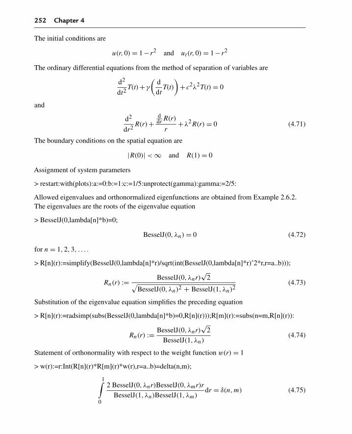
252 Chapter 4
The initial conditions are
u(r,0) = 1− r2 and ut(r,0) = 1− r2
The ordinary differential equations from the method of separation of variables are
d2
dt2T(t)+γ
(d
dtT(t)
)+ c2λ2T(t) = 0
and
d2
dr2R(r)+
ddr
R(r)
r+λ2R(r) = 0 (4.71)
The boundary conditions on the spatial equation are
|R(0)| < ∞ and R(1) = 0
Assignment of system parameters
> restart:with(plots):a:=0:b:=1:c:=1/5:unprotect(gamma):gamma:=2/5:
Allowed eigenvalues and orthonormalized eigenfunctions are obtained from Example 2.6.2.The eigenvalues are the roots of the eigenvalue equation
> BesselJ(0,lambda[n]*b)=0;
BesselJ(0, λn) = 0 (4.72)
for n = 1,2,3, . . . .
> R[n](r):=simplify(BesselJ(0,lambda[n]*r)/sqrt(int(BesselJ(0,lambda[n]*r)ˆ2*r,r=a..b)));
Rn(r) := BesselJ(0, λnr)√
2√BesselJ(0, λn)2 + BesselJ(1, λn)2
(4.73)
Substitution of the eigenvalue equation simplifies the preceding equation
> R[n](r):=radsimp(subs(BesselJ(0,lambda[n]*b)=0,R[n](r)));R[m](r):=subs(n=m,R[n](r)):
Rn(r) := BesselJ(0, λnr)√
2
BesselJ(1, λn)(4.74)
Statement of orthonormality with respect to the weight function w(r) = 1
> w(r):=r:Int(R[n](r)*R[m](r)*w(r),r=a..b)=delta(n,m);
1∫0
2 BesselJ(0, λnr)BesselJ(0, λmr)r
BesselJ(1, λn)BesselJ(1, λm)dr = δ(n,m) (4.75)

The Wave Partial Differential Equation 253
Time-dependent solution
> T[n](t):=exp((−gamma/2)*t)*(A(n)*cos(omega[n]*t)+B(n)*sin(omega[n]*t));
Tn(t) := e−15 t
(A(n) cos(ωnt)+B(n) sin(ωnt)) (4.76)
Generalized series terms
> u[n](r,t):=T[n](t)*R[n](r):
Eigenfunction expansion
> u(r,t):=Sum(u[n](r,t),n=1..infinity);
u(r, t) :=∞∑
n=1
e−15 t
(A(n) cos(ωnt)+B(n) sin(ωnt)) BesselJ(0, λnr)√
2
BesselJ(1, λn)(4.77)
> omega[n]:=sqrt(lambda[n]ˆ2*cˆ2−gammaˆ2/4);
ωn := 1
5
√λ2
n −1 (4.78)
From Section 4.8, the coefficients A(n) and B(n) are to be determined from the inner productof the eigenfunctions and the initial condition functions u(r,0) = f(r) and ut(r,0) = g(r).
> f(r):=1−rˆ2;
f(r) := 1− r2 (4.79)
> g(r):=1−rˆ2;
g(r) := 1− r2 (4.80)
For n = 1,2,3, . . . ,
> A(n):=eval(Int(f(r)*R[n](r)*w(r),r=a..b));A(n):=value(%):
A(n) :=1∫
0
(1− r2) BesselJ(0, λnr)√
2 r
BesselJ(1, λn)dr (4.81)
Substitution of the eigenvalue equation simplifies the preceding equation
> A(n):=simplify(subs(BesselJ(0,lambda[n]*b)=0,A(n)));
A(n) := 4√
2
λ3n
(4.82)
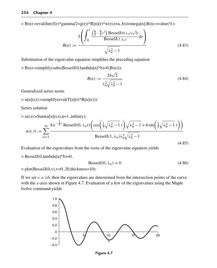
254 Chapter 4
> B(n):=eval(Int((f(r)*gamma/2+g(r))*R[n](r)*w(r),r=a..b))/omega[n];B(n):=value(%):
B(n) :=5
⎛⎝
∫ 1
0
(65−6
5 r2)
BesselJ(0,λnr)√
2r
BesselJ(1,λn)dr
⎞⎠
√λ2
n −1(4.83)
Substitution of the eigenvalue equation simplifies the preceding equation
> B(n):=simplify(subs(BesselJ(0,lambda[n]*b)=0,B(n)));
B(n) := 24√
2
λ3n
√λ2
n −1(4.84)
Generalized series terms
> u[n](r,t):=simplify(eval(T[n](t)*R[n](r))):
Series solution
> u(r,t):=Sum(u[n](r,t),n=1..infinity);
u(r, t) :=∞∑
n=1
8 e−15 t BesselJ(0, λnr)
(cos
(15
√λ2
n −1 t
)√λ2
n −1+6 sin
(15
√λ2
n −1 t
))
BesselJ(1, λn)λ3n
√λ2
n −1
(4.85)Evaluation of the eigenvalues from the roots of the eigenvalue equation yields
> BesselJ(0,lambda[n]*b)=0;
BesselJ(0, λn) = 0 (4.86)> plot(BesselJ(0,v),v=0..20,thickness=10);
If we set v = λb, then the eigenvalues are determined from the intersection points of the curvewith the v-axis shown in Figure 4.7. Evaluation of a few of the eigenvalues using the Maplefsolve command yields
10 15 20
20.4
20.2
0
0.2
0.4
0.6
0.8
1.0
5
v
Figure 4.7

The Wave Partial Differential Equation 255
> lambda[1]:=(1/b)*fsolve(BesselJ(0,v)=0,v=0..3);
λ1 := 2.404825558 (4.87)
> lambda[2]:=(1/b)*fsolve(BesselJ(0,v)=0,v=3..6);
λ2 := 5.520078110 (4.88)
> lambda[3]:=(1/b)*fsolve(BesselJ(0,v)=0,v=6..9);
λ3 := 8.653727913 (4.89)
First few terms in sum
> u(r,t):=eval(sum(u[n](r,t),n=1..3)):
ANIMATION
> animate(u(r,t),r=a..b,t=0..2,thickness=3);
The preceding animation command illustrates the spatial-time-dependent solution for u(r, t).The following animation sequence in Figure 4.8 shows snapshots of the animation at timest = 0,1,2,3,4, and 5.
ANIMATION SEQUENCE
> u(r,0):=subs(t=0,u(r,t)):u(r,1):=subs(t=1,u(r,t)):> u(r,2):=subs(t=2,u(r,t)):u(r,3):=subs(t=3,u(r,t)):> u(r,4):=subs(t=4,u(r,t)):u(r,5):=subs(t=5,u(r,t)):> plot({u(r,0),u(r,1),u(r,2),u(r,3),u(r,4),u(r,5)},r=a..b,thickness=10);
r0 0.2 0.4 0.6 0.8 1
0
0.6
1
1.4
1.8
Figure 4.8
THREE-DIMENSIONAL ANIMATION
> u(x,y,t):=eval(subs(r=sqrt(xˆ2+yˆ2),u(r,t))):> u(x,y,t):=(u(x,y,t))*Heaviside(1−sqrt(xˆ2+yˆ2)):> animate3d(u(x,y,t),x=−b..b,y=−b..b,t=0..10,axes=framed,thickness=1);

256 Chapter 4
EXAMPLE 4.9.2: We consider transverse vibrations in a thin circularly symmetric membraneover the interval I = {r |0 < r < 1}, which is unsecured at the periphery. The membranevibrates in a medium with very small damping. The membrane has an initial displacementdistribution f(r) and an initial speed distribution g(r) given as follows. The wave speed isc = 1/5, and the damping factor is γ = 2/5.
SOLUTION: The homogeneous wave equation is
∂2
∂t2u(r, t)+γ
(∂
∂tu(r, t)
)=
c2(
∂∂r u(r, t)+ r
(∂2
∂r2 u(r, t)))
r
The boundary conditions are type 2 at r = 1 and a finite solution at r = 0
|u(0, t)| < ∞ and ur(1, t) = 0
The initial conditions are
u(r,0) = 1− r2 and ut(r,0) = 1− r2
The ordinary differential equations from the method of separation of variables are
d2
dt2T(t)+γ
(d
dtT(t)
)+ c2λ2T(t) = 0
and
d2
dr2R(r)+
ddr
R(r)
r+λ2R(r) = 0 (4.90)
The boundary conditions on the spatial equation are
|R(0)| < ∞ and Rr(1) = 0
Assignment of system parameters
> restart:with(plots):a:=0:b:=1:c:=1/5:unprotect(gamma):gamma:=2/5:
Allowed eigenvalues and orthonormalized eigenfunctions are obtained from Example 2.6.3.
> lambda[0]:=0;
λ0 := 0 (4.91)
for n = 0.
> R[0](r):=sqrt(2)/b;
R0(r) := √2 (4.92)
For n = 1,2,3, . . . , the eigenvalues are the roots of the eigenvalue equation
The Wave Partial Differential Equation 257
> subs(r=b,diff(BesselJ(0,lambda[n]*r),r)=0);
−BesselJ(1, λn)λn = 0 (4.93)
> R[n](r):=simplify(BesselJ(0,lambda[n]*r)/sqrt(int(BesselJ(0,lambda[n]*r)ˆ2*r,r=a..b)));
Rn(r) := BesselJ(0, λnr)√
2√BesselJ(0, λn)2 + BesselJ(1, λn)2
(4.94)
Substitution of the eigenvalue equation simplifies the preceding equation
> R[n](r):=radsimp(subs(BesselJ(1,lambda[n]*b)=0,R[n](r)));R[m](r):=subs(n=m,R[n](r)):
Rn(r) := BesselJ(0, λnr)√
2
BesselJ(0, λn)(4.95)
Statement of orthonormality with respect to the weight function w(r) = r
> w(r):=r:Int(R[n](r)*R[m](r)*w(r),r=a..b)=delta(n,m);
1∫0
2 BesselJ(0, λnr) BesselJ(0, λmr)r
BesselJ(0, λn) BesselJ(0, λm)dr = δ(n,m) (4.96)
Time-dependent solution
> T[0](t):=A(0)+B(0)*exp(−gamma*t);
T0(t) := A(0)+B(0)e−25 t (4.97)
for n = 0.
> T[n](t):=exp((−gamma/2)*t)*(A(n)*cos(omega[n]*t)+B(n)*sin(omega[n]*t));
Tn(t) := e−15 t
(A(n) cos(ωnt)+B(n) sin(ωnt)) (4.98)
for n = 1,2,3, . . . .
Generalized series terms
> u[0](r,t):=eval(T[0](t)*R[0](r)):u[n](r,t):=eval(T[n](t)*R[n](r)):
Eigenfunction expansion
> u(r,t):=u[0](r,t)+Sum(u[n](r,t),n=1..infinity);
u(r, t) :=(
A(0)+B(0)e−25 t
)√2
+∞∑
n=1
e−15 t
(A(n) cos(ωnt)+B(n) sin(ωnt)) BesselJ(0, λnr)√
2
BesselJ(0, λn)(4.99)

258 Chapter 4
> omega[n]:=sqrt(lambda[n]ˆ2*cˆ2−gammaˆ2/4);
ωn := 1
5
√λ2
n −1 (4.100)
From Section 4.8, the coefficients A(n) and B(n) are to be determined from the inner productof the eigenfunctions and the initial condition functions u(r,0) = f(r) and ut(r,0) = g(r).
> f(r):=1−rˆ2;
f(r) := 1− r2 (4.101)
> g(r):=1−rˆ2;
g(r) := 1− r2 (4.102)
For n = 0,
> A(0):=Int((f(r)*gamma+g(r))/gamma*R[0](r)*w(r),r=a..b);
A(0) :=1∫
0
5
2
(7
5− 7
5r2
)√2 r dr (4.103)
> A(0):=value(%);
A(0) := 7
8
√2 (4.104)
> B(0):=Int((−1/gamma)*g(r)*R[0](r)*w(r),r=a..b);
B(0) :=1∫
0
(−5
2(1− r2)
√2 r
)dr (4.105)
> B(0):=value(%);
B(0) := −5
8
√2 (4.106)
For n = 1,2,3, . . . ,
> A(n):=Int(f(r)*R[n](r)*w(r),r=a..b);
A(n) :=1∫
0
(1− r2) BesselJ(0, λnr)√
2 r
BesselJ(0, λn)dr (4.107)
Substitution of the eigenvalue equation simplifies the preceding equation
> A(n):=subs(BesselJ(1,lambda[n]*b)=0,value(%));
A(n) := −2√
2
λ2n
(4.108)
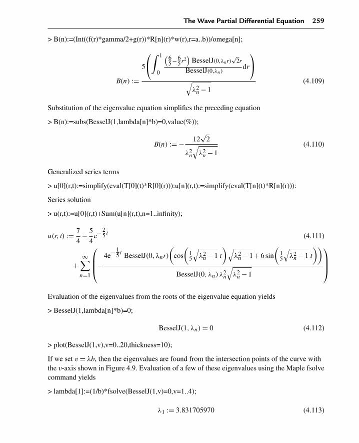
The Wave Partial Differential Equation 259
> B(n):=(Int((f(r)*gamma/2+g(r))*R[n](r)*w(r),r=a..b))/omega[n];
B(n) :=5
⎛⎝
∫ 1
0
(65−6
5 r2)
BesselJ(0,λnr)√
2r
BesselJ(0,λn)dr
⎞⎠
√λ2
n −1(4.109)
Substitution of the eigenvalue equation simplifies the preceding equation
> B(n):=subs(BesselJ(1,lambda[n]*b)=0,value(%));
B(n) := − 12√
2
λ2n
√λ2
n −1(4.110)
Generalized series terms
> u[0](r,t):=simplify(eval(T[0](t)*R[0](r))):u[n](r,t):=simplify(eval(T[n](t)*R[n](r))):
Series solution
> u(r,t):=u[0](r,t)+Sum(u[n](r,t),n=1..infinity);
u(r, t) := 7
4− 5
4e−2
5 t (4.111)
+∞∑
n=1
⎛⎜⎜⎝−
4e−15 t BesselJ(0, λnr)
(cos
(15
√λ2
n −1 t
)√λ2
n −1+6 sin
(15
√λ2
n −1 t
))
BesselJ(0, λn)λ2n
√λ2
n −1
⎞⎟⎟⎠
Evaluation of the eigenvalues from the roots of the eigenvalue equation yields
> BesselJ(1,lambda[n]*b)=0;
BesselJ(1, λn) = 0 (4.112)
> plot(BesselJ(1,v),v=0..20,thickness=10);
If we set v = λb, then the eigenvalues are found from the intersection points of the curve withthe v-axis shown in Figure 4.9. Evaluation of a few of these eigenvalues using the Maple fsolvecommand yields
> lambda[1]:=(1/b)*fsolve(BesselJ(1,v)=0,v=1..4);
λ1 := 3.831705970 (4.113)
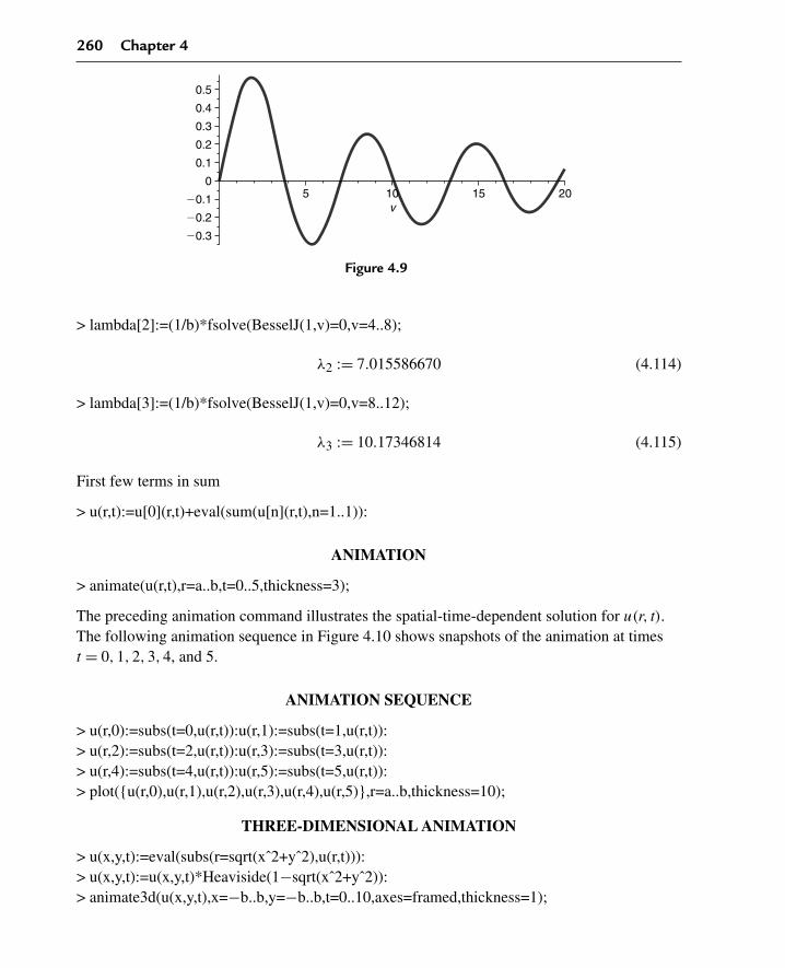
260 Chapter 4
v5 15 20
20.3
20.2
20.1
0
0.1
0.2
0.3
0.4
0.5
10
Figure 4.9
> lambda[2]:=(1/b)*fsolve(BesselJ(1,v)=0,v=4..8);
λ2 := 7.015586670 (4.114)
> lambda[3]:=(1/b)*fsolve(BesselJ(1,v)=0,v=8..12);
λ3 := 10.17346814 (4.115)
First few terms in sum
> u(r,t):=u[0](r,t)+eval(sum(u[n](r,t),n=1..1)):
ANIMATION
> animate(u(r,t),r=a..b,t=0..5,thickness=3);
The preceding animation command illustrates the spatial-time-dependent solution for u(r, t).The following animation sequence in Figure 4.10 shows snapshots of the animation at timest = 0,1,2,3,4, and 5.
ANIMATION SEQUENCE
> u(r,0):=subs(t=0,u(r,t)):u(r,1):=subs(t=1,u(r,t)):> u(r,2):=subs(t=2,u(r,t)):u(r,3):=subs(t=3,u(r,t)):> u(r,4):=subs(t=4,u(r,t)):u(r,5):=subs(t=5,u(r,t)):> plot({u(r,0),u(r,1),u(r,2),u(r,3),u(r,4),u(r,5)},r=a..b,thickness=10);
THREE-DIMENSIONAL ANIMATION
> u(x,y,t):=eval(subs(r=sqrt(xˆ2+yˆ2),u(r,t))):> u(x,y,t):=u(x,y,t)*Heaviside(1−sqrt(xˆ2+yˆ2)):> animate3d(u(x,y,t),x=−b..b,y=−b..b,t=0..10,axes=framed,thickness=1);

The Wave Partial Differential Equation 261
r0.0 0.2 0.4 0.6 0.8 1
0.40.60.8
11.21.41.61.8
Figure 4.10
Chapter Summary
Nonhomogeneous wave equation of dimension one in rectangular coordinates
∂2
∂t2u(x, t) = c2
(∂2
∂x2u(x, t)
)−γ
(∂
∂tu(x, t)
)+h(x, t)
Linear wave operator in rectangular coordinates of dimension one
L(u) = ∂2
∂t2u(x, t)− c2
(∂2
∂x2u(x, t)
)+γ
(∂
∂tu(x, t)
)
Method of separation of variables solution
u(x, t) = X(x)T(t)
Eigenfunction expansion solution
u(x, t) =∞∑
n=0
Xn(x)e−γt2 (A(n) cos(ωnt)+B(n) sin(ωnt))
Nonhomogeneous wave equation of dimension one in cylindrical coordinates
∂2
∂t2u(r, t) =
c2(
∂∂r u(r, t)+ r
(∂2
∂r2 u(r, t)))
r−γ
(∂
∂tu(r, t)
)+h(r, t)
Linear wave operator in cylindrical coordinates of dimension one
L(u) = ∂2
∂t2u(r, t)−
c2(
∂∂r u(r, t)+ r
(∂2
∂r2 u(r, t)))
r+γ
(∂
∂tu(r, t)
)
Method of separation of variables solution
u(r, t) = R(r)T(t)

262 Chapter 4
Eigenfunction expansion solution
u(r, t) =∞∑
n=0
Rn(r)e−γt2 (A(n) cos(ωnt)+B(n) sin(ωnt))
We have examined solutions to the wave partial differential equation in a single spatialdimension for both the rectangular and the polar-cylindrical coordinate systems. We willexamine these same partial differential equations in steady-state and higher-dimensionalsystems later.
Exercises
We now consider wave equations with homogeneous boundary conditions in both therectangular and cylindrical coordinate systems. Use the method of separation of variables andeigenfunction expansions to evaluate the solutions to the following exercises.
Exercises in Rectangular Coordinates
4.1. Consider the transverse wave motion on a taut string over the finite intervalI = {x |0 < x < 1} in a slightly damped medium. The homogeneous partial differentialequation reads as
∂2
∂t2u(x, t) = c2
(∂2
∂x2u(x, t)
)−γ
(∂
∂tu(x, t)
)
with c = 1/4, γ = 1/5, and boundary conditions
u(0, t) = 0 and u(1, t) = 0
The left end and the right end are held fixed. The initial conditions are
u(x,0) = f(x) and ut(x,0) = g(x)
Evaluate the eigenvalues and corresponding orthonormalized eigenfunctions, and writethe general solution. Evaluate the solution for each of the four sets of initial conditionsgiven:
f1(x) = 1 and g1(x) = 0
f2(x) = x and g2(x) = 1
f3(x) = x(1−x) and g3(x) = 0
The plucked string. For 0 < x < 1/2,
f4(x) = x and g4(x) = 0

The Wave Partial Differential Equation 263
For 1/2 < x < 1,
f4(x) = 1−x and g4(x) = 0
Generate the animated solution for each case, and plot the animated sequence for0 < t < 5.
4.2. Consider longitudinal wave motion in a bar over the finite interval I = {x |0 < x < 1}with a slight amount of damping. The homogeneous partial differential equationreads as
∂2
∂t2u(x, t) = c2
(∂2
∂x2u(x, t)
)−γ
(∂
∂tu(x, t)
)
with c = 1/5, γ = 1/5, and boundary conditions
u(0, t) = 0 and ux(1, t) = 0
The left end is secured and the right end is unsecured. The initial conditions are
u(x,0) = f(x) and ut(x,0) = g(x)
Evaluate the eigenvalues and corresponding orthonormalized eigenfunctions, and writethe general solution. Evaluate the solution for each of the three sets of initial conditionsgiven:
f1(x) =(
x− 1
2
)2and g1(x) = 0
f2(x) = x and g2(x) = 1
f3(x) = x(
1− x
2
)and g3(x) = 0
Generate the animated solution for each case, and plot the animated sequence for0 < t < 5.
4.3. Consider longitudinal wave motion in a bar over the finite interval I = {x|0 < x < 1}with a slight amount of damping. The homogeneous partial differential equation reads as
∂2
∂t2u(x, t) = c2
(∂2
∂x2u(x, t)
)−γ
(∂
∂tu(x, t)
)
with c = 1/4, γ = 1/5, and boundary conditions
ux(0, t) = 0 and u(1, t) = 0
The left end is unsecured and the right end is secured. The initial conditions are
u(x,0) = f(x) and ut(x,0) = g(x)

264 Chapter 4
Evaluate the eigenvalues and corresponding orthonormalized eigenfunctions, and writethe general solution. Evaluate the solution for each of the three sets of initial conditionsgiven:
f1(x) = x and g1(x) = 0
f2(x) = 1 and g2(x) = 1
f3(x) = 1−x2 and g3(x) = 0
Generate the animated solution for each case, and plot the animated sequence for0 < t < 5.
4.4. Consider longitudinal wave motion in a bar over the finite interval I = {x |0 < x < 1}with a slight amount of damping. The homogeneous partial differential equation reads as
∂2
∂t2u(x, t) = c2
(∂2
∂x2u(x, t)
)−γ
(∂
∂tu(x, t)
)
with c = 1/4, γ = 1/5, and boundary conditions
ux(0, t) = 0 and ux(1, t) = 0
The left end and the right end are unsecured. The initial conditions are
u(x,0) = f(x),ut(x,0) = g(x)
Evaluate the eigenvalues and corresponding orthonormalized eigenfunctions, and writethe general solution. Evaluate the solution for each of the three sets of initial conditionsgiven:
f1(x) = x and g1(x) = 0
f2(x) = 1−x2 and g2(x) = 1
f3(x) = x2(
1− 2x
3
)and g3(x) = 0
Generate the animated solution for each case, and plot the animated sequence for0 < t < 5.
4.5. Consider longitudinal wave motion in a bar over the finite interval I = {x |0 < x < 1}with a slight amount of damping. The homogeneous partial differential equationreads as
∂2
∂t2u(x, t) = c2
(∂2
∂x2u(x, t)
)−γ
(∂
∂tu(x, t)
)

The Wave Partial Differential Equation 265
with c = 1/4, γ = 1/5, and boundary conditions
u(0, t) = 0 and ux(1, t)+u(1, t) = 0
The left end is secured and the right end is attached to an elastic hinge. The initialconditions are
u(x,0) = f(x) and ut(x,0) = g(x)
Evaluate the eigenvalues and corresponding orthonormalized eigenfunctions, and writethe general solution. Evaluate the solution for each of the three sets of initial conditionsgiven:
f1(x) = 1 and g1(x) = 0
f2(x) = x and g2(x) = 1
f3(x) = x
(1− 2x
3
)and g3(x) = 0
Generate the animated solution for each case, and plot the animated sequence for0 < t < 5.
4.6. Consider longitudinal wave motion in a bar over the finite interval I = {x |0 < x < 1}with a slight amount of damping. The homogeneous partial differential equationreads as
∂2
∂t2u(x, t) = c2
(∂2
∂x2u(x, t)
)−γ
(∂
∂tu(x, t)
)
with c = 1/4, γ = 1/5, and boundary conditions
ux(0, t)−u(0, t) = 0 and u(1, t) = 0
The left end is attached to an elastic hinge and the right end is secured. The initialconditions are
u(x,0) = f(x) and ut(x,0) = g(x)
Evaluate the eigenvalues and corresponding orthonormalized eigenfunctions, and writethe general solution. Evaluate the solution for each of the three sets of initial conditionsgiven:
f1(x) = 1 and g1(x) = 0
f2(x) = 1−x and g2(x) = 1
f3(x) = −2x2
3+ x
3+ 1
3and g3(x) = 0

266 Chapter 4
Generate the animated solution for each case, and plot the animated sequence for0 < t < 5.
4.7. Consider longitudinal wave motion in a bar over the finite interval I = {x |0 < x < 1}with a slight amount of damping. The homogeneous partial differential equationreads as
∂2
∂t2u(x, t) = c2
(∂2
∂x2u(x, t)
)−γ
(∂
∂tu(x, t)
)
with c = 1/4, γ = 1/5, and boundary conditions
ux(0, t) = 0 and ux(1, t)+u(1, t) = 0
The left end is unsecured and the right end is attached to an elastic hinge. The initialconditions are
u(x,0) = f(x) and ut(x,0) = g(x)
Evaluate the eigenvalues and corresponding orthonormalized eigenfunctions, and writethe general solution. Evaluate the solution for each of the three sets of initial conditionsgiven:
f1(x) = x and g1(x) = 0
f2(x) = 1 and g2(x) = 1
f3(x) = 1− x2
3and g3(x) = 0
Generate the animated solution for each case, and plot the animated sequence for0 < t < 5.
4.8. Consider longitudinal wave motion in a bar over the finite interval I = {x |0 < x < 1}with a slight amount of damping. The homogeneous partial differential equationreads as
∂2
∂t2u(x, t) = c2
(∂2
∂x2u(x, t)
)−γ
(∂
∂tu(x, t)
)
with c = 1/4, γ = 1/5, and boundary conditions
ux(0, t)−u(0, t) = 0 and ux(1, t) = 0
The left end is attached to an elastic hinge and the right end is unsecured. The initialconditions are
u(x,0) = f(x) and ut(x,0) = g(x)

The Wave Partial Differential Equation 267
Evaluate the eigenvalues and corresponding orthonormalized eigenfunctions, and writethe general solution. Evaluate the solution for each of the three sets of initial conditionsgiven:
f1(x) = x and g1(x) = 0
f2(x) = 1 and g2(x) = 1
f3(x) = 1− (x−1)2
3and g3(x) = 0
Generate the animated solution for each case, and plot the animated sequence for0 < t < 5.
4.9. We consider the transverse wave motion along a taut string over the finite intervalI = {x |0 < x < 1}. In addition to slight damping, the string is immersed in a mediumthat provides a restoring force that is proportional to the displacement of the string(Hooke’s law–type of force). The resulting partial differential equation is called the“telegraph” equation:
∂2
∂t2u(x, t) = c2
(∂2
∂x2u(x, t)
)−γ
(∂
∂tu(x, t)
)− ζu(x, t)
with c = 1/4, γ = 1/5, ζ = 1/10, and boundary conditions
u(0, t) = 0 and u(1, t) = 0
The left end of the string and the right end of the string are secured. The initialconditions are
u(x,0) = f(x) and ut(x,0) = g(x)
Use the method of separation of variables to evaluate the eigenvalues andcorresponding orthonormalized eigenfunctions, and write the general solution. Evaluatethe solution for each of the three sets of initial conditions given:
f1(x) = 1 and g1(x) = 0
f2(x) = x and g2(x) = 1
f3(x) = x(x−1) and g3(x) = 0
Generate the animated solution for each case, and plot the animated sequence for0 < t < 5.
268 Chapter 4
4.10. We again consider the telegraph partial differential equation over the finite intervalI = {x |0 < x < 1}.
∂2
∂t2u(x, t) = c2
(∂2
∂x2u(x, t)
)−γ
(∂
∂tu(x, t)
)− ζu(x, t)
with c = 1/4, γ = 1/5, ζ = 1/10, and boundary conditions
u(0, t) = 0 and ux(1, t) = 0
The left end of the string is secured and the right end of the string is unsecured. Theinitial conditions are
u(x,0) = f(x) and ut(x,0) = g(x)
Use the method of separation of variables to evaluate the eigenvalues andcorresponding orthonormalized eigenfunctions, and write the general solution. Evaluatethe solution for each of the three sets of initial conditions given:
f1(x) =(
x− 1
2
)2and g1(x) = 0
f2(x) = x and g2(x) = 1
f3(x) = x
(1− x
2
)and g3(x) = 0
Generate the animated solution for each case, and plot the animated sequence for0 < t < 5.
4.11. We again consider the telegraph partial differential equation over the finite intervalI = {x |0 < x < 1}.
∂2
∂t2u(x, t) = c2
(∂2
∂x2u(x, t)
)−γ
(∂
∂tu(x, t)
)− ζu(x, t)
with c = 1/4, γ = 1/5, ζ = 1/10, and boundary conditions
u(0, t) = 0 and ux(1, t)+u(1, t) = 0
The left end of the string is secured, and the right end of the string is attached to anelastic hinge. The initial conditions are
u(x,0) = f(x) and ut(x,0) = g(x)

The Wave Partial Differential Equation 269
Use the method of separation of variables to evaluate the eigenvalues andcorresponding orthonormalized eigenfunctions, and write the general solution. Evaluatethe solution for each of the three sets of initial conditions given:
f1(x) = 1 and g1(x) = 0
f2(x) = x and g2(x) = 1
f3(x) = x
(1− 2x
3
)and g3(x) = 0
Generate the animated solution for each case, and plot the animated sequence for0 < t < 5.
4.12. We again consider the telegraph partial differential equation over the finite intervalI = {x |0 < x < 1}. The telegraph equation reads as
∂2
∂t2u(x, t) = c2
(∂2
∂x2u(x, t)
)−γ
(∂
∂tu(x, t)
)− ζu(x, t)
with c = 1/4, γ = 1/5, ζ = 1/10, and boundary conditions
ux(0, t)−u(0, t) = 0 and u(1, t) = 0
The left end of the string is attached to an elastic hinge, and the right end of the string issecured. The initial conditions are
u(x,0) = f(x) and ut(x,0) = g(x)
Use the method of separation of variables to evaluate the eigenvalues andcorresponding orthonormalized eigenfunctions, and write the general solution. Evaluatethe solution for each of the three sets of initial conditions given:
f1(x) = 1 and g1(x) = 0
f2(x) = 1−x and g2(x) = 1
f3(x) = −2x2
3+ x
3+ 1
3and g3(x) = 0
Generate the animated solution for each case, and plot the animated sequence for0 < t < 5.
4.13. Here, we consider the transverse wave motion along a taut string over the finite intervalI = {x |0 < x < 1}. The damping on the string is negligible, and the string is immersedin a medium that provides a restoring force that is proportional to the displacement of

270 Chapter 4
the string (Hooke’s law–type of force). The resulting partial differential equation iscalled the “Klein-Gordon” equation:
∂2
∂t2u(x, t) = c2
(∂2
∂x2u(x, t)
)− ζu(x, t)
with c = 1/4, ζ = 1/10, and boundary conditions
ux(0, t) = 0 and u(1, t) = 0
The left end of the string is unsecured and the right end of the string is secured. Theinitial conditions are
u(x,0) = f(x) and ut(x,0) = g(x)
Use the method of separation of variables to evaluate the eigenvalues andcorresponding orthonormalized eigenfunctions, and write the general solution. Evaluatethe solution for each of the three sets of initial conditions given:
f1(x) = x and g1(x) = 0
f2(x) = 1 and g2(x) = 1
f3(x) = 1−x2 and g3(x) = 0
Generate the animated solution for each case, and plot the animated sequence for0 < t < 5.
4.14. We again consider the Klein-Gordon equation for transverse wave motion along a tautstring over the finite interval I = {x |0 < x < 1}. The Klein-Gordon equation reads
∂2
∂t2u(x, t) = c2
(∂2
∂x2u(x, t)
)− ζu(x, t)
with c = 1/4, ζ = 1/10, and boundary conditions
ux(0, t) = 0 and ux(1, t)+u(1, t) = 0
The left end of the string is unsecured, and the right end of the string is attached to anelastic hinge. The initial conditions are
u(x,0) = f(x) and ut(x,0) = g(x)
Use the method of separation of variables to evaluate the eigenvalues andcorresponding orthonormalized eigenfunctions, and write the general solution. Evaluate

The Wave Partial Differential Equation 271
the solution for each of the three sets of initial conditions given:
f1(x) = x and g1(x) = 0
f2(x) = 1 and g2(x) = 1
f3(x) = 1− x2
3and g3(x) = 0
Generate the animated solution for each case, and plot the animated sequence for0 < t < 5.
4.15. We again consider the Klein-Gordon equation for transverse wave motion along a tautstring over the finite interval I = {x |0 < x < 1}. The Klein-Gordon equation is
∂2
∂t2u(x, t) = c2
(∂2
∂x2u(x, t)
)− ζu(x, t)
with c = 1/4, ζ = 1/10, and boundary conditions
ux(0, t)−u(0, t) = 0 and ux(1, t) = 0
The left end of the string is attached to an elastic hinge, and the right end of the string isunsecured. The initial conditions are
u(x,0) = f(x) and ut(x,0) = g(x)
Use the method of separation of variables to evaluate the eigenvalues, andcorresponding orthonormalized eigenfunctions, and write the general solution. Evaluatethe solution for each of the three sets of initial conditions given:
f1(x) = x and g1(x) = 0
f2(x) = 1 and g2(x) = 1
f3(x) = 1− (x−1)2
3and g3(x) = 0
Generate the animated solution for each case, and plot the animated sequence for0 < t < 5.
Exercises in Cylindrical Coordinates
4.16. Consider the transverse vibrations in a thin circularly symmetric membrane over thefinite interval I = {r |0 < r <1 with a slight amount of damping. The homogeneouspartial differential equation reads as
∂2
∂t2u(r, t) =
c2
(∂
∂ru(r, t)+ r
(∂2
∂r2u(r, t)
))
r−γ
(∂
∂tu(r, t)
)
272 Chapter 4
with c = 1/4, γ = 1/5, and boundary conditions
|u(0, t)| < ∞ and u(1, t) = 0
The center of the membrane has a finite amplitude, and the periphery of the membraneis secure. The initial conditions are
u(r,0) = f(r) and ut(r,0) = g(r)
Evaluate the eigenvalues and corresponding orthonormalized eigenfunctions, and writethe general solution. Evaluate the solution for the three sets of initial conditions given:
f1(r) = r2 and g1(r) = 0
f2(r) = 1 and g2(r) = 1
f3(r) = 1− r2 and g3(r) = 0
Generate the animated solution for each case, and plot the animated sequence for0 < t < 5.
4.17. Consider the transverse vibrations in a thin circularly symmetric membrane over thefinite interval I = {r |0 < r < 1} with a slight amount of damping. The homogeneouspartial differential equation reads as
∂2
∂t2u(r, t) =
c2
(∂
∂ru(r, t)+ r
(∂2
∂r2u(r, t)
))
r−γ
(∂
∂tu(r, t)
)
with c = 1/4, γ = 1/5, and boundary conditions
|u(0, t)| < ∞ and ur(1, t) = 0
The center of the membrane has a finite amplitude, and the periphery of the membraneis unsecured. The initial conditions are
u(r,0) = f(r) and ut(r,0) = g(r)
Evaluate the eigenvalues and corresponding orthonormalized eigenfunctions, and writethe general solution. Evaluate the solution for the three sets of initial conditions given:
f1(r) = r2 and g1(r) = 0
f2(r) = 1 and g2(r) = 1
f3(r) = r2 − r4
2and g3(r) = 0
Generate the animated solution for each case, and plot the animated sequence for0 < t < 5.

The Wave Partial Differential Equation 273
4.18. Consider the transverse vibrations in a thin circularly symmetric membrane over thefinite interval I = {r |0 < r < 1} with a slight amount of damping. The homogeneouspartial differential equation reads as
∂2
∂t2u(r, t) =
c2
(∂
∂ru(r, t)+ r
(∂2
∂r2u(r, t)
))
r−γ
(∂
∂tu(r, t)
)
with c = 1/4, γ = 1/5, and boundary conditions
|u(0, t)| < ∞ and ur(1, t)+u(1, t) = 0
The center of the membrane has a finite amplitude, and the periphery of the membraneis attached to an elastic hinge. The initial conditions are
u(r,0) = f(r) and ut(r,0) = g(r)
Evaluate the eigenvalues and corresponding orthonormalized eigenfunctions, and writeout the general solution. Evaluate the solution for the three sets of initial conditionsgiven:
f1(r) = r2 and g1(r) = 0
f2(r) = 1 and g2(r) = 1
f3(r) = 1− r2
3and g3(r) = 0
Generate the animated solution for each case, and plot the animated sequence for0 < t < 5.
Significance of Wave SpeedThe speed of propagation of the wave in the preceding exercises was indicated by thefactor c. (This speed is not to be confused with the speed of motion of the particles thatmake up the medium and whose collective motion constitutes the wave.) In thepreceding exercises, we assumed the medium to be homogeneous and isotropic so thatall terms that evaluate c are treated as constants.
In the case of transverse waves on a taut string, the constant c is given as
c =√
To
ρ

274 Chapter 4
where To is the tension in the string and ρ is the linear density of the string. In the caseof longitudinal waves in a bar, the constant c is given as
c =√
Eo
ρ
where Eo is the Young’s modulus of elasticity and ρ is the mass density of the bar. Inthe case of transverse waves in a membrane, the constant c is given as
c =√
To
ρ
where To is the tension per unit length in the membrane and ρ is the areal density (massper unit area) of the membrane. In the MKS system, wave speed has dimensions ofmeters per second.
In the following exercises, you are asked to multiply the speed term by a given factorand to develop the solution for the initial conditions set {f3(x), g3(x)}. Develop theanimated solution, and take particular note of how the increase in wave speed affectsthe vibration frequency of the various modes of vibration of the medium.
4.19. In Exercise 4.2, multiply the speed term c by a factor of 2 and solve.
4.20. In Exercise 4.4, multiply the speed term c by a factor of 4 and solve.
4.21. In Exercise 4.7, multiply the speed term c by a factor of 2 and solve.
4.22. In Exercise 4.9, multiply the speed term c by a factor of 4 and solve.
4.23. In Exercise 4.13, multiply the speed term c by a factor of 2 and solve.
4.24. In Exercise 4.16, multiply the speed term c by a factor of 4 and solve.
4.25. In Exercise 4.17, multiply the speed term c by a factor of 2 and solve.

CHAPTER 5
The Laplace Partial DifferentialEquation
5.1 Introduction
The Laplace partial differential equation can be shown to be the steady-state equivalent ofeither the wave equation or the diffusion equation. In electrostatics, the Laplace equationdescribes the potential in a charge-free region, and, for this reason, it is sometimes called the“potential” equation.
In Chapter 3, we discussed the diffusion or heat partial differential equation in rectangularcoordinates in one spatial dimension with no internal sources. If we view the spatial derivativeoperator as the first term of the Laplacian operator, then an extension of this diffusionequation from one to two spatial dimensions reads
∂
∂tu(x, y, t) = k
(∂2
∂x2u(x, y, t)+ ∂2
∂y2u(x, y, t)
)
If we consider the steady-state or time-invariant version of this equation, we get
∂2
∂x2u(x, y)+ ∂2
∂y2u(x, y) = 0
The preceding partial differential equation is the familiar homogeneous Laplace partialdifferential equation in the two-dimensional rectangular coordinate system.
In Chapter 4, we discussed the wave partial differential equation in rectangular coordinates inone spatial dimension with no damping in the system and no external applied forces. Again, ifwe view the spatial derivative operator as the first term of the Laplacian operator, then anextension of the wave equation from one to two spatial dimensions reads
∂2
∂t2u(x, y, t) = c2
(∂2
∂x2u(x, y, t)+ ∂2
∂y2u(x, y, t)
)
© 2009, 2003, 1999 Elsevier Inc. 275

276 Chapter 5
Again, if we consider the steady-state or time-invariant version of this equation, we get
∂2
∂x2u(x, y)+ ∂2
∂y2u(x, y) = 0
Thus, we see that in the steady-state situation, both the diffusion and the wave partialdifferential equation reduce to the familiar Laplace equation.
A typical example steady-state problem is as follows. We seek the steady-state temperaturedistribution u(x,y) in a thin plate over the rectangular domain D = {(x,y) |0 < x < 1,0 < y < 1}. The lateral surfaces of the plate are insulated so that no heat escapes from thelateral surfaces. The sides y = 0 and y = 1 are insulated, the side x = 1 has a fixed temperatureof zero, and the side x = 0 has a temperature distribution f(y) given as follows.
The Laplace partial differential equation that describes the steady-state temperature in theplate is
∂2
∂x2u(x, y)+ ∂2
∂y2u(x, y) = 0
Because the sides y = 0 and y = 1 are insulated, the side x = 0 is at a fixed temperature zero,and the side x = 0 has a given temperature distribution, the boundary conditions on theproblem are
u(0, y) = f(y) and u(1, y) = 0
and
uy(x,0) = 0 and uy(x,1) = 0
We develop the solution for this problem in Section 5.3 later.
5.2 Laplace Equation in the Rectangular Coordinate System
We now focus on the solution to the Laplace equation over the finite two-dimensional domainD = {(x,y) |0 < x < a,0 < y < b} in rectangular coordinates. From the preceding section,the relevant partial differential equation can be rewritten to read
∂2
∂x2u(x, y) = −
(∂2
∂y2u(x, y)
)
Based on our success in solving the diffusion equation and the wave equation in Chapters 3and 4, we use the method of separation of variables to solve this equation. We set
u(x, y) = X(x)Y(y)

The Laplace Partial Differential Equation 277
Substituting this assumed solution into the partial differential equation, we get
(d2
dx2X(x)
)Y(y) = −X(x)
(d2
dy2Y(y)
)
Dividing the preceding by the product solution yields
d2
dx2X(x)
X(x)= −
d2
dy2Y(y)
Y(y)
Because the left-hand side of the equation is an exclusive function of x and the right-hand sideis an exclusive function of y, and x and y are independent, then in order for the equation tohold for all x and y, we must set each side equal to a constant λ. Doing so gives us thefollowing two ordinary differential equations:
d2
dx2X(x)+λX(x) = 0
and
d2
dy2Y(y)−λY(y) = 0
Both of these ordinary differential equations are of the Euler type. To proceed further, we nowconsider the boundary conditions on the problem. Generally, one seeks a solution to thisproblem over the finite two-dimensional domain D = {(x,y) |0 < x < a,0 < y < b} subject tothe regular homogeneous boundary conditions on one of the variables, x or y. We seek thatvariable whose boundary conditions are homogeneous.
For example, consider the case where the boundary conditions on u(x,y) are homogeneouswith respect to the x variable:
κ1u(0, y)+κ2ux(0, y) = 0
and
κ3u(a, y)+κ4ux(a, y) = 0 (5.1)
The earlier ordinary differential equation in x, combined with the equivalent homogeneousboundary conditions, constitutes a Sturm-Liouville problem in the variable x, for which wealready have solutions.

278 Chapter 5
5.3 Sturm-Liouville Problem for the Laplace Equation inRectangular Coordinates
The differential equation in the spatial variable x in the preceding equation must be solvedsubject to the equivalent homogeneous spatial boundary conditions over the finite interval. TheSturm-Liouville problem for the x-dependent equation consists of the ordinary differentialequation
d2
dx2X(x)+λX(x) = 0
along with the equivalent corresponding homogeneous boundary conditions on the x variableas shown here:
κ1X(0)+κ2Xx(0) = 0
and
κ3X(a)+κ4Xx(a) = 0
We recognize this problem in the spatial variable x to be a regular Sturm-Liouville eigenvalueproblem whereby the allowed values of λ are called the system “eigenvalues” and thecorresponding solutions are called the “eigenfunctions.” Note that the preceding ordinarydifferential equation is of the Euler type with the weight function w(x) = 1.
As before, it can be shown that for regular Sturm-Liouville problems over finite domains, aninfinite number of eigenvalues exists that can be indexed by the integer numbers n. Theindexed eigenvalues and corresponding eigenfunctions are given, respectively, as
λn,Xn(x)
for n = 0,1,2,3, . . . .
From the stated properties of regular Sturm-Liouville eigenvalue problems in Section 2.1, theeigenfunctions form a “complete” set with respect to any piecewise smooth function over thefinite x-dependent interval I = {x |0 < x < a}.From Section 1.4 on second-order linear differential equations, the solution to thecorresponding y-dependent differential equation in terms of the allowed eigenvalues is
Yn(y) = A(n) cosh(√
λny)
+B(n) sinh(√
λny)
Thus, for each allowed value of the index n, we have a solution
un(x, y) = Xn(x)(A(n) cosh
(√λny
)+B(n) sinh
(√λny
))for n = 0,1,2,3, . . . .

The Laplace Partial Differential Equation 279
These functions form a set of basis vectors for the solution space of the partial differentialequation. Using the same concepts of the superposition principle as in Chapters 3 and 4, thegeneral solution to the homogeneous partial differential equation can now be written as aninfinite sum over all basis vectors as follows:
u(x, y) =∞∑
n=0
Xn(x)(A(n) cosh
(√λny
)+B(n) sinh
(√λny
))
The arbitrary constants A(n) and B(n) are evaluated by taking advantage of the orthonormalityof the x-dependent eigenfunctions over the finite interval I = {x |0 < x < a}, with respect tothe weight function w(x) = 1. The statement of orthonormality reads
a∫0
Xn(x)Xm(x)dx = δ(n,m)
for n,m = 0,1,2,3, . . . .
We mentioned earlier that in using the method of separation of variables successfully, we mustseek out that variable, x or y, that experiences the homogeneous boundary conditions. In thepreceding, conditions on x forced it to be that variable.
We now consider the alternative possibility. If the homogeneous boundary conditions onu(x,y) are on the variable y instead of x, then we rewrite the two earlier ordinary differentialequations as
d2
dx2X(x)−λX(x) = 0
and
d2
dy2Y(y)+λY(y) = 0
The homogeneous boundary conditions on u(x,y) with respect to the variable y are as shown:
κ1u(x,0)+κ2uy(x,0) = 0
and
κ3u(x, b)+κ4uy(x, b) = 0
The given ordinary differential equation on y, combined with the preceding equivalent regularhomogeneous boundary conditions, again constitutes a Sturm-Liouville problem, in terms ofthe variable y, for which we already have solutions.
280 Chapter 5
The differential equation in the spatial variable y must be solved subject to the homogeneousspatial boundary conditions over the finite interval. The Sturm-Liouville problem for they-dependent equation consists of the ordinary differential equation
d2
dy2Y(y)+λY(y) = 0
along with the equivalent corresponding homogeneous boundary conditions on y shown:
κ1Y(0)+κ2Yy(0) = 0
and
κ3Y(b)+κ4Yy(b) = 0
Again, we see this problem in the spatial variable y to be a regular Sturm-Liouville eigenvalueproblem whereby the allowed values of λ are called the system “eigenvalues” and thecorresponding solutions are called the “eigenfunctions.” Note that the preceding ordinarydifferential equation is of the Euler type and the weight function is w(y) = 1.
As before, we can show that for regular Sturm-Liouville problems over finite domains, aninfinite number of eigenvalues exist that can be indexed by the positive integers n. The indexedeigenvalues and corresponding eigenfunctions are given, respectively, as
λn,Yn(y)
for n = 0,1,2,3, . . . .
Again, from the stated properties of regular Sturm-Liouville eigenvalue problems inSection 2.1, the eigenfunctions form a “complete” set with respect to any piecewise smoothfunction over the finite y-dependent interval I = {y |0 < y < b}.From Section 1.4 on second-order linear differential equations, the solution to thecorresponding x-dependent differential equation in terms of the allowed eigenvalues is
Xn(x) = A(n) cosh(√
λnx)
+B(n) sinh(√
λnx)
(5.2)
Thus, for each allowed value of the index n, we have a solution
un(x, y) = Yn(y)(A(n) cosh
(√λx
)+B(n) sinh
(√λx
))for n = 0,1,2,3, . . . .
Using the concept of the superposition principle as in Chapters 3 and 4, the general solution tothe homogeneous partial differential equation can again be written as the infinite sum of thepreceding basis vectors in terms of the eigenfunctions with respect to the variable y as follows:
u(x, y) =∞∑
n=0
Yn(y)(A(n) cosh
(√λnx
)+B(n) sinh
(√λnx
))

The Laplace Partial Differential Equation 281
Again, the arbitrary constants A(n) and B(n) can be evaluated by taking advantage of theorthonormality of the y-dependent eigenfunctions, with respect to the weight functionw(y) = 1 over the interval I = {y |0 < y < b}. The statement of orthonormality reads
b∫0
Yn(y)Ym(y)dy = δ(n,m) (5.3)
for n,m = 0,1,2,3, . . . .
The boundary conditions on the problem determine whether the solution is written in terms ofthe eigenfunctions with respect to x or y. Remember that the decision comes from our seekingthat particular variable that experiences the homogeneous boundary conditions.
DEMONSTRATION: We seek the steady-state temperature distribution in a thin rectangularplate over the rectangular domain D = {(x,y) |0 < x < 1,0 < y < 1}. The lateral surfaces ofthe plate are insulated. The sides y = 0 and y = 1 are insulated. The side x = 1 has a fixedtemperature of zero, and the side x = 0 has a temperature distribution f(y) given as follows.
SOLUTION: The Laplace partial differential equation is
∂2
∂x2u(x, y)+ ∂2
∂y2u(x, y) = 0
The boundary conditions are
u(0, y) = f(y) and u(1, y) = 0
and
uy(x,0) = 0 and uy(x,1) = 0
We seek that variable whose boundary conditions are homogeneous. Here, we see that thehomogeneous boundary conditions are with respect to the y variable. Thus, by the method ofseparation of variables, we write the two ordinary differential equations as
d2
dx2X(x)−λX(x) = 0
and
d2
dy2Y(y)+λY(y) = 0
Because both ends along the y-axis are insulated, the corresponding homogeneous boundaryconditions on the y equation are type 2 at y = 0 and type 2 at y = 1.
Yy(0) = 0 and Yy(1) = 0

282 Chapter 5
The allowed eigenvalues and corresponding orthonormal eigenfunctions are obtained fromExample 2.5.3 in Chapter 2. For λ0 = 0, we got
Y0(y) = 1
and for λn = n2π2, we got
Yn(y) = √2 cos(nπy)
for n = 1,2,3, . . . .
The statement of orthonormality with respect to the weight function w(y) = 1 reads
1∫0
2 cos(nπy) cos(mπy)dy = δ(n,m)
for n,m = 1,2,3, . . . .
A set of basis vectors for the x-dependent equation for λn = n2π2 reads
x1(x) = sinh(nπ(1−x))
and
x2(x) = cosh(nπ(1−x))
and the general solution to the x equation is
Xn(x) = A(n) cosh(nπ(1−x))+B(n) sinh(nπ(1−x))
Substitution of the boundary condition at x = 1 yields A(n) = 0. Thus, the solution for thex-dependent equation is
Xn(x) = B(n) sinh(nπ(1−x))
for n = 1,2,3, . . . .
Similarly, for λ0 = 0, a set of basis vectors is
x1(x) = 1
and
x2(x) = x
and a solution that satisfies the boundary condition at x = 1 reads
X0(x) = B(0)(1−x)

The Laplace Partial Differential Equation 283
The generalized eigenfunction expansion of the solution is constructed from the sum of theproduct of the x-dependent solutions and the preceding orthonormal y-dependenteigenfunctions. This yields
u(x, y) = B(0)(1−x)+∞∑
n=1
B(n) sinh(nπ(1−x))√
2 cos(nπy)
The Fourier coefficients B(n) are determined from the remaining boundary condition.Substitution of the boundary condition u(0, y) = f(y) at x = 0 yields
f(y) = B(0)+∞∑
n=1
B(n) sinh(nπ)√
2 cos(nπy)
This equation is the Fourier series expansion of f(y) in terms of the orthonormal y-dependentSturm-Liouville eigenfunctions found earlier. To evaluate the Fourier coefficients B(n), wetake the inner product of both sides with respect to the orthonormal eigenfunctions, and takingadvantage of the statement of orthonormality, we get
B(n) =
∫ 1
0f(y)
√2 cos(nπy)dy
sinh(nπ)
for n = 1,2,3, . . . , and
B(0) =1∫
0
f(y)dy
for n = 0.
We consider the special case for the boundary condition along x = 0 to be f(y) = y(1−y). Theintegral for B(n) reads
B(n) =
∫ 1
0y(1−y)
√2 cos(nπy)dy
sinh(nπ)
Evaluation of this integral yields
B(n) = −√
2((−1)n +1
)sinh(nπ)n2π2
for n = 1,2,3, . . . .
Similarly, for n = 0, the integral for B(0) reads
B(0) =1∫
0
y(1−y)dy

284 Chapter 5
Evaluation of this integral yields
B(0) = 1
6
Finally, the solution for the steady-state temperature of the system is
u(x, y) = 1−x
6+
∞∑n=1
(−2
((−1)n +1
)sinh(nπ(1−x)) cos(nπy)
sinh(nπ)n2π2
)
The detailed development of this solution and the graphics are given later in one of the Mapleworksheet examples.
5.4 Example Laplace Problems in the RectangularCoordinate System
We look at steady-state solutions to wave and diffusion phenomena in the two-dimensional,rectangular coordinate (x,y) plane. We assume conditions such that there is no dependence ofthe solution on the z coordinate.
EXAMPLE 5.4.1: We seek the electrostatic potential in a charge-free rectangular domainD = {(x,y) |0 < x < 1,0 < y < 1}. The sides x = 0, x = 1, and y = 1 are held at a fixedpotential zero, and the side y = 0 has a potential distribution u(x,0) = f(x) given below.
SOLUTION: The homogeneous Laplace equation is
∂2
∂x2u(x, y)+ ∂2
∂y2u(x, y) = 0
The boundary conditions are
u(0, y) = 0 and u(1, y) = 0
and
u(x,0) = x(1−x) and u(x,1) = 0
Here, we see that the boundary conditions are homogeneous with respect to the x variable.
Ordinary differential equations from the method of separation of variables are
d2
dx2X(x)+λX(x) = 0
and
d2
dy2Y(y)−λY(y) = 0

The Laplace Partial Differential Equation 285
Homogeneous boundary conditions on the x equation are type 1 at x = 0 and type 1 at x = 1
X(0) = 0 and X(1) = 0
Assignment of system parameters
> restart:with(plots):a:=1:b:=1:
Allowed eigenvalues and corresponding orthonormal eigenfunctions for the x equation areobtained from Example 2.5.1.
> lambda[n]:=(n*Pi/a)ˆ2;
λn := n2π2 (5.4)
for n = 1,2,3, . . . .
Orthonormal eigenfunctions
> X[n](x):=sqrt(2/a)*sin(n*Pi/a*x);X[n](s):=subs(x=s,X[n](x)):X[m](x):=subs(n=m,X[n](x)):
Xn(x) := √2 sin(nπx) (5.5)
Statement of orthonormality with respect to the weight function w(x) = 1
> w(x):=1:Int(X[n](x)*X[m](x)*w(x),x=0..a)=delta(n,m);
1∫0
2 sin(nπx) sin(mπx)dx = δ(n,m) (5.6)
Basis vectors for the y equation
> y1(y):=sinh(sqrt(lambda)*(b−y));y2(y):=cosh(sqrt(lambda)*(b−y));
y1(y) := sinh(√
λ(1−y))
y2(y) := cosh(√
λ(1−y))
(5.7)
General solution to the y equation
> Y[n](y):=A(n)*cosh(n*Pi/a*(b−y))+B(n)*sinh(n*Pi/a*(b−y));
Yn(y) := A(n) cosh(nπ(1−y))+B(n) sinh(nπ(1−y)) (5.8)
Substituting into the y-dependent boundary condition yields
> eval(subs(y=b,Y[n](y)))=0;
A(n) = 0 (5.9)

286 Chapter 5
The y-dependent solution
> Y[n](y):=B(n)*sinh(n*Pi/a*(b−y));
Yn(y) := B(n) sinh(nπ(1−y)) (5.10)
Generalized series terms
> u[n](x,y):=X[n](x)*Y[n](y);
un(x, y) := √2 sin(nπx)B(n) sinh(nπ(1−y)) (5.11)
Eigenfunction expansion
> u(x,y):=Sum(u[n](x,y),n=1..infinity);
u(x, y) :=∞∑
n=1
√2 sin(nπx)B(n) sinh(nπ(1−y)) (5.12)
Evaluation of Fourier coefficients from the specific remaining boundary conditionu(x,0) = f(x) where
> f(x):=x*(1−x);
f(x) := x(1−x) (5.13)
Substituting this condition into the earlier solution yields
> f(x)=subs(y=0,u(x,y));
x(1−x) =∞∑
n=1
√2 sin(nπx)B(n) sinh(nπ) (5.14)
The preceding equation is the Fourier series expansion of f(x) in terms of the orthonormalSturm-Liouville eigenfunctions found earlier. To evaluate the Fourier cofficients, we take theinner product of both sides with respect to the orthonormal eigenfunctions, and, takingadvantage of the previous statement of orthonormality, we get
> B(n):=(1/sinh(n*Pi*b/a))*Int(f(x)*X[n](x)*w(x),x=0..a);B(n):=expand(value(%)):
B(n) :=
∫ 1
0x(1−x)
√2 sin(nπx)dx
sinh(nπ)(5.15)
Evaluation of this integral yields
> B(n):=simplify(subs({sin(n*Pi)=0,cos(n*Pi)=(−1)ˆn},B(n)));
B(n) := −2√
2(−1+ (−1)n
)sinh(nπ)n3π3
(5.16)

The Laplace Partial Differential Equation 287
Generalized series terms
> u[n](x,y):=eval(X[n](x)*Y[n](y));
un(x, y) := −4 sin(nπx)(−1+ (−1)n
)sinh(nπ(1−y))
sinh(nπ)n3π3 (5.17)
Series solution
> u(x,y):=Sum(u[n](x,y),n=1..infinity);
u(x, y) :=∞∑
n=1
(−4 sin(nπx)(−1+ (−1)n) sinh(nπ(1−y))
sinh(nπ)n3π3
)(5.18)
First few terms of expansion
> u(x,y):=sum(u[n](x,y),n=1..5):
> plot3d(u(x,y),x=0..a,y=0..b,axes=framed,thickness=1);
0.25
0.150.1
0.05
0.2
00
0.20.4
0.60.8
1 10.8
0.60.4
xy
0.20
Figure 5.1
The three-dimensional surface shown in Figure 5.1 depicts the electrostatic potentialdistribution u(x, y) over the rectangular region. Note how the edges of the surface adhere to thegiven boundary conditions. The equipotential lines can be obtained from Maple by clicking onthe figure and then choosing the special option “Render the plot using the polygon patch andcontour style” in the graphics bar and then clicking the “redraw” button.
EXAMPLE 5.4.2: We seek the steady-state temperature distribution in a thin rectangular plateover the domain D = {(x, y) |0 < x < 1,0 < y < 1} whose lateral surface is insulated. Thesides y = 0 and y = 1 are insulated, the side x = 1 has a fixed temperature of zero, and the sidex = 0 follows the temperature distribution u(0, y) = f(y) given as follows.
SOLUTION: The homogeneous Laplace equation is
∂2
∂x2u(x, y)+ ∂2
∂y2u(x, y) = 0

288 Chapter 5
The boundary conditions are
u(0, y) = y(1−y) and u(1, y) = 0
and
uy(x,0) = 0 and uy(x,1) = 0
Here, we see that the boundary conditions are homogeneous with respect to the y variable.
Ordinary differential equations from the method of separation of variables are
d2
dx2X(x)−λX(x) = 0
and
d2
dy2Y(y)+λY(y) = 0
Homogeneous boundary conditions on the y equation are type 2 at y = 0 and type 2 at y = 1
Yy(0) = 0 and Yy(1) = 0
Assignment of system parameters
> restart:with(plots):a:=1:b:=1:
Allowed eigenvalues and corresponding orthonormal eigenfunctions for the y equation areobtained from Example 2.5.3. For n = 0,
> lambda[0]:=0;
λ0 := 0 (5.19)
Orthonormal eigenfunction
> Y[0](y):=1/sqrt(b);
Y0(y) := 1 (5.20)
For n = 1,2,3, . . . ,
> lambda[n]:=(n*Pi/b)ˆ2;
λn := n2π2 (5.21)
Orthonormal eigenfunctions
> Y[n](y):=sqrt(2/b)*cos(n*Pi/b*y);Y[n](s):=subs(y=s,Y[n](y)):Y[m](y):=subs(n=m,Y[n](y)):
Yn(y) := √2 cos(nπy) (5.22)

The Laplace Partial Differential Equation 289
Statement of orthonormality with respect to the weight function w(y) = 1
> w(y):=1:Int(Y[n](y)*Y[m](y)*w(y),y=0..b)=delta(n,m);
1∫0
2 cos(nπy) cos(mπy)dy = δ(n,m) (5.23)
Basis vectors for the x equation
> x1(x):=sinh(sqrt(lambda)*(a−x));x2(x):=cosh(sqrt(lambda)*(a−x));
x1(x) := sinh(√
λ(1−x))
x2(x) := cosh(√
λ(1−x))
(5.24)
General solution to the x equation for n = 1,2,3, . . .
> X[n](x):=A(n)*cosh(n*Pi/b*(a−x))+B(n)*sinh(n*Pi/b*(a−x));
Xn(x) := A(n) cosh(nπ(1−x))+B(n) sinh(nπ(1−x)) (5.25)
Substituting into the x-dependent boundary condition yields
> eval(subs(x=a,X[n](x)))=0;
A(n) = 0 (5.26)
For n = 1,2,3, . . . , we have for the x-dependent solution
> X[n](x):=B(n)*sinh(n*Pi/b*(a−x));
Xn(x) := B(n) sinh(nπ(1−x)) (5.27)
Similarly, for n = 0, the x-dependent solution is
> X[0](x):=B(0)*(a−x);
X0(x) := B(0)(1−x) (5.28)
Generalized series terms
> u[0](x,y):=X[0](x)*Y[0](y);u[n](x,y):=X[n](x)*Y[n](y);
u0(x, y) := B(0)(1−x)
un(x, y) := B(n) sinh(nπ(1−x))√
2 cos(nπy) (5.29)

290 Chapter 5
Eigenfunction expansion
> u(x,y):=u[0](x,y)+Sum(u[n](x,y),n=1..infinity);
u(x, y) := B(0)(1−x)+∞∑
n=1
B(n) sinh(nπ(1−x))√
2 cos(nπy) (5.30)
Evaluation of Fourier coefficients from the specific remaining boundary conditionu(0, y) = f(y)
> f(y):=y*(1−y);
f(y) := y(1−y) (5.31)
Substituting this condition into the preceding solution yields
> f(y)=subs(x=0,u(x,y));
y(1−y) = B(0)+∞∑
n=1
B(n) sinh(nπ)√
2 cos(nπy) (5.32)
This equation is the Fourier series expansion of f(y) in terms of the orthonormalSturm-Liouville eigenfunctions found earlier. To evaluate the Fourier cofficients, we take theinner product of both sides with respect to the orthonormal eigenfunctions, and, takingadvantage of the previous statement of orthonormality, we get
> B(n):=(1/sinh(n*Pi*a/b))*Int(f(y)*Y[n](y)*w(y),y=0..b);B(n):=expand(value(%)):
B(n) :=
∫ 1
0y(1−y)
√2 cos(nπy)dy
sinh(nπ)(5.33)
> B(n):=simplify(subs({sin(n*Pi)=0,cos(n*Pi)=(−1)ˆn},B(n)));
B(n) := −√
2(1+ (−1)n)
sinh(nπ)n2π2(5.34)
for n = 1,2,3, . . . . Similarly, for n = 0, we get
> B(0):=eval((1/a)*Int(f(y)*Y[0](y)*w(y),y=0..b));B(0):=value(%):
B(0) :=1∫
0
y(1−y)dy (5.35)
> B(0):=subs({sin(n*Pi)=0,cos(n*Pi)=(−1)ˆn},B(0));
B(0) := 1
6(5.36)

The Laplace Partial Differential Equation 291
Generalized series terms
> u[0](x,y):=eval(X[0](x)*Y[0](y));u[n](x,y):=eval(X[n](x)*Y[n](y));
u0(x, y) := 1
6− 1
6x
un(x, y) := −2(1+ (−1)n) sinh(nπ(1−x)) cos(nπy)
sinh(nπ)n2π2(5.37)
Series solution
> u(x,y):=u[0](x,y)+Sum(u[n](x,y),n=1..infinity);
u(x, y) := 1
6− 1
6x+
∞∑n=1
(−2(1+ (−1)n) sinh(nπ(1−x)) cos(nπy)
sinh(nπ)n2π2
)(5.38)
First few terms of expansion
> u(x,y):=sum(u[0](x,y)+u[n](x,y),n=1..5):
> plot3d(u(x,y),x=0..a,y=0..b,axes=framed,thickness=1);
0.80.60.40.2
00
0.20.4
0.60.8
1
y
10.8
0.60.4x
0.20
Figure 5.2
The three-dimensional surface shown in Figure 5.2 depicts the steady-state temperaturedistribution u(x, y) over the rectangular region. Note how the edges of the surface adhere tothe given boundary conditions. The temperature isotherms can be obtained from Maple byclicking on the figure, choosing the special option “Render the plot using the polygon patchand contour style” in the graphics bar, and then clicking the “redraw” button.
EXAMPLE 5.4.3: We seek the steady-state temperature distribution in a thin rectangular plateover the domain D = {(x, y) |0 < x < 1,0 < y < 1} whose lateral surface is insulated. The sidey = 1 is insulated, the sides x = 1 and y = 0 are held at a fixed temperature of zero, and theside x = 0 follows the temperature distribution u(0, y) = f(y) given as follows.
292 Chapter 5
SOLUTION: The homogeneous Laplace equation is
∂2
∂x2u(x, y)+ ∂2
∂y2u(x, y) = 0
The boundary conditions are
u(0, y) = y(1−y) and u(1, y) = 0
and
u(x,0) = 0 and uy(x,1) = 0
Here, we see that the boundary conditions are homogeneous with respect to the y variable.
Ordinary differential equations from the method of separation of variables are
d2
dx2X(x)−λX(x) = 0
and
d2
dy2Y(y)+λY(y) = 0
Homogeneous boundary conditions on the y equation are type 1 at y = 0 and type 2 at y = 1
Y(0) = 0 and Yy(1) = 0
Assignment of system parameters
> restart:with(plots):a:=1:b:=1:
Allowed eigenvalues and corresponding orthonormal eigenfunctions for the y equation areobtained from Example 2.5.2.
> lambda[n]:=((2*n−1)*Pi/(2*b))ˆ2;
λn := 1
4(2n−1)2π2 (5.39)
for n = 1,2,3, . . . .
Orthonormal eigenfunctions
> Y[n](y):=sqrt(2/b)*sin((2*n−1)*Pi/(2*b)*y);Y[m](y):=subs(n=m,Y[n](y)):
Yn(y) := √2 sin
(1
2(2n−1)πy
)(5.40)
Statement of orthonormality with respect to the weight function w(y) = 1

The Laplace Partial Differential Equation 293
> w(y):=1:Int(Y[n](y)*Y[m](y)*w(y),y=0..b)=delta(n,m);
1∫0
2 sin
(1
2(2n−1)πy
)sin
(1
2(2m−1)πy
)dy = δ(n,m) (5.41)
Basis vectors for the x equation
> x1(x):=sinh(sqrt(lambda)*(a−x));x2(x):=cosh(sqrt(lambda)*(a−x));
x1(x) := sinh(√
λ(1−x))
x2(x) := cosh(√
λ(1−x))
(5.42)
General solution to the x equation
> X[n](x):=A(n)*cosh((2*n−1)*Pi/(2*b)*(a−x))+B(n)*sinh((2*n−1)*Pi/(2*b)*(a−x));
Xn(x) := A(n) cosh
(1
2(2n−1)π(1−x)
)+B(n) sinh
(1
2(2n−1)π(1−x)
)(5.43)
Substituting into the x-dependent boundary condition yields
> eval(subs(x=a,X[n](x)))=0;
A(n) = 0 (5.44)
The x-dependent solution
> X[n](x):=B(n)*sinh((2*n−1)*Pi/(2*b)*(a−x));
Xn(x) := B(n) sinh
(1
2(2n−1)π(1−x)
)(5.45)
Generalized series terms
> u[n](x,y):=X[n](x)*Y[n](y);
un(x, y) := B(n) sinh
(1
2(2n−1)π(1−x)
)√2 sin
(1
2(2n−1)πy
)(5.46)
Eigenfunction expansion
> u(x,y):=Sum(u[n](x,y),n=1..infinity);
u(x, y) :=∞∑
n=1
B(n) sinh
(1
2(2n−1)π(1−x)
)√2 sin
(1
2(2n−1)πy
)(5.47)
Evaluation of Fourier coefficients from the specific remaining boundary conditionu(0, y) = f(y)

294 Chapter 5
> f(y):=y*(1−y);
f(y) := y(1−y) (5.48)
Substituting this condition into the preceding solution yields
> f(y)=subs(x=0,u(x,y));
y(1−y) =∞∑
n=1
B(n) sinh
(1
2(2n−1)π
)√2 sin
(1
2(2n−1)πy
)(5.49)
The preceding equation is the Fourier series expansion of f(y) in terms of the orthonormalizedSturm-Liouville eigenfunctions found earlier. To evaluate the Fourier cofficients, we take theinner product of both sides with respect to the orthonormalized eigenfunctions, and, takingadvantage of the previous statement of orthonormality, we get, for n = 1,2,3, . . . ,
> B(n):=(1/sinh((2*n−1)*Pi*a/(2*b)))*Int(f(y)*Y[n](y)*w(y),y=0..b);B(n):=value(%):
B(n) :=∫ 1
0 y(1−y)√
2 sin(
12(2n−1)πy
)dy
sinh(
12(2n−1)π
) (5.50)
> B(n):=simplify(subs({sin(n*Pi)=0,cos(n*Pi)=(−1)ˆn,sin((2*n+1)*Pi/2)=(−1)ˆn,cos((2*n+1)*Pi/2)=0},B(n)));
B(n) := 4√
2(4+2πn(−1)n −π(−1)n)
sinh(
12(2n−1)π
)π3(8n3 −12n2 +6n−1)
(5.51)
Generalized series terms
> u[n](x,y):=eval(X[n](x)*Y[n](y));
un(x, y) :=8(4+2πn(−1)n −π(−1)n) sinh
(12(2n−1)π(1−x)
)sin
(12(2n−1)πy
)sinh
(12(2n−1)π
)π3(8n3 −12n2 +6n−1)
(5.52)
Series solution
> u(x,y):=Sum(u[n](x,y),n=1..infinity);
u(x, y) :=∞∑
n=1
8(4+2πn(−1)n −π(−1)n) sinh(
12(2n−1)π(1−x)
)sin
(12(2n−1)πy
)sinh
(12(2n−1)π
)π3(8n3 −12n2 +6n−1)
(5.53)First few terms of expansion
> u(x,y):=sum(u[n](x,y),n=1..5):> plot3d(u(x,y),x=0..a,y=0..b,axes=framed,thickness=1);

The Laplace Partial Differential Equation 295
0.20.150.1
00
0.20.4y 0.6
1 10.8
0.60.4
x
0.20
0.8
0.05
Figure 5.3
The three-dimensional surface shown in Figure 5.3 depicts the steady-state temperaturedistribution u(x, y) over the rectangular region. Note how the edges of the surface adhere tothe given boundary conditions. The temperature isotherms can be obtained from Maple byclicking on the figure, choosing the special option “Render the plot using the polygon patchand contour style” in the graphics bar, and then clicking the “redraw” button.
EXAMPLE 5.4.4: We seek the steady-state temperature distribution in a thin rectangular plateover the domain D = {(x, y) |0 < x < 1,0 < y < 1} whose lateral surface is insulated. The sidex = 0 is insulated, the side y = 1 has a fixed temperature of zero, the side y = 0 follows thetemperature distribution f(x), and the side x = 1 is experiencing a convection heat loss into azero temperature surrounding.
SOLUTION: The homogeneous Laplace equation is
∂2
∂x2u(x, y)+ ∂2
∂y2u(x, y) = 0
The boundary conditions are
ux(0, y) = 0 and u(1, y)+ux(1, y) = 0
and
u(x,0) = 1−x2 and u(x,1) = 0
Here, we see that the boundary conditions are homogeneous with respect to the x variable.
Ordinary differential equations from the method of separation of variables are
d2
dx2X(x)+λX(x) = 0
and
d2
dy2Y(y)−λY(y) = 0

296 Chapter 5
Homogeneous boundary conditions on the x equation are type 2 at x = 0 and type 3 at x = 1:
Xx(0) = 0 and Xx(1)+X(1) = 0
Assignment of system parameters
> restart:with(plots):a:=1:b:=1:
Allowed eigenvalues and corresponding orthonormal eigenfunctions for the x equation areobtained from Example 2.5.5. The eigenvalues are the roots of the eigenvalue equation
> tan(sqrt(lambda[n])*a)=1/sqrt(lambda[n]);
tan(√
λn
)= 1√
λn(5.54)
for n = 1,2,3, . . . .
Orthonormal eigenfunctions
> X[n](x):=sqrt(2)*cos(sqrt(lambda[n])*x)/sqrt(((sin(sqrt(lambda[n])*a))ˆ2+a));X[m](x):=subs(n=m,X[n](x)):
Xn(x) :=√
2 cos(√
λn x)
√sin
(√λn
)2 +1(5.55)
Statement of orthonormality with respect to the weight function w(x) = 1
> w(x):=1:Int(X[n](x)*X[m](x)*w(x),x=0..a)=delta(n,m);
1∫0
2 cos(√
λn x)
cos(√
λm x)
√sin
(√λn
)2 +1√
sin(√
λm
)2 +1dx = δ(n,m) (5.56)
Basis vectors for the y equation
> y1(y):=sinh(sqrt(lambda)*(b−y));y2(y):=cosh(sqrt(lambda)*(b−y));
y1(y) := sinh(√
λ(1−y))
y2(y) := cosh(√
λ(1−y))
(5.57)
General solution to the y equation
> Y[n](y):=A(n)*cosh(sqrt(lambda[n])*(b−y))+B(n)*sinh(sqrt(lambda[n])*(b−y));
Yn(y) := A(n) cosh(√
λn(1−y))
+B(n) sinh(√
λn(1−y))
(5.58)

The Laplace Partial Differential Equation 297
Substituting into the y-dependent boundary condition yields
> eval(subs(y=b,Y[n](y)))=0;
A(n) = 0 (5.59)
The y-dependent solution
> Y[n](y):=B(n)*sinh(sqrt(lambda[n])*(b−y));
Yn(y) := B(n) sinh(√
λn(1−y))
(5.60)
> u[n](x,y):=X(n)(x)*Y[n](y):
Eigenfunction expansion
> u(x,y):=Sum(u[n](x,y),n=1..infinity);
u(x, y) :=∞∑
n=1
√2 cos
(√λnx
)B(n) sinh
(√λn(1−y)
)√
sin(√
λn
)2 +1(5.61)
Evaluation of Fourier coefficients from the specific remaining boundary conditionu(x,0) = f(x)
> f(x):=1−xˆ2;
f(x) := 1−x2 (5.62)
Substituting this condition into the preceding solution yields
> f(x)=subs(y=0,u(x,y));
1−x2 =∞∑
n=1
√2 cos
(√λnx
)B(n) sinh
(√λn
)√
sin(√
λn
)2 +1(5.63)
This equation is the Fourier series expansion of f(x) in terms of the orthonormalSturm-Liouville eigenfunctions found earlier. To evaluate the Fourier coefficients, we take theinner product of both sides with respect to the orthonormal eigenfunctions, and, takingadvantage of the previous statement of orthonormality, we get, for n = 1,2,3, . . . ,
> B(n):=(1/sinh(sqrt(lambda[n])*b))*Int(f(x)*X[n](x)*w(x),x=0..a);B(n):=value(%):
B(n) :=
∫ 1
0
(1−x2)√
2 cos(√
λnx)√
sin(√
λn
)2+1dx
sinh(√
λn
) (5.64)
Substitution of the eigenvalue equation simplifies the preceding equation
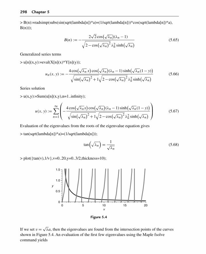
298 Chapter 5
> B(n):=radsimp(subs(sin(sqrt(lambda[n])*a)=(1/sqrt(lambda[n]))*cos(sqrt(lambda[n])*a),B(n)));
B(n) := − 2√
2 cos(√
λn
)(λn −1)√
2− cos(√
λn
)2λ2
n sinh(√
λn
) (5.65)
Generalized series terms
> u[n](x,y):=eval(X[n](x)*Y[n](y));
un(x, y) := −4 cos(√
λn x)
cos(√
λn
)(λn −1) sinh
(√λn(1−y)
)√
sin(√
λn
)2 +1√
2− cos(√
λn
)2λ2
n sinh(√
λn
) (5.66)
Series solution
> u(x,y):=Sum(u[n](x,y),n=1..infinity);
u(x, y) :=∞∑
n=1
⎛⎜⎝−4 cos
(√λnx
)cos
(√λn
)(λn −1) sinh
(√λn(1−y)
)√
sin(√
λn
)2 +1√
2− cos(√
λn
)2λ2
n sinh(√
λn
)⎞⎟⎠ (5.67)
Evaluation of the eigenvalues from the roots of the eigenvalue equation gives
> tan(sqrt(lambda[n])*a)=(1/sqrt(lambda[n]));
tan(√
λn
)= 1√
λn(5.68)
> plot({tan(v),1/v},v=0..20,y=0..3/2,thickness=10);
5 10v
y
15 2000
0.5
1.0
1.5
Figure 5.4
If we set v = √λa, then the eigenvalues are found from the intersection points of the curves
shown in Figure 5.4. An evaluation of the first few eigenvalues using the Maple fsolvecommand yields

The Laplace Partial Differential Equation 299
> lambda[1]:=(1/aˆ2)*(fsolve((tan(v)−1/v),v=0..1))ˆ2;
λ1 := 0.7401738844 (5.69)
> lambda[2]:=(1/aˆ2)*(fsolve((tan(v)−1/v),v=1..4))ˆ2;
λ2 := 11.73486183 (5.70)
> lambda[3]:=(1/aˆ2)*(fsolve((tan(v)−1/v),v=4..7))ˆ2;
λ3 := 41.43880785 (5.71)
First few terms of expansion
> u(x,y):=sum(u[n](x,y),n=1..3):
> plot3d(u(x,y),x=0..a,y=0..b,axes=framed,thickness=1);
0.80.60.4
00
0.20.4y 0.6
1 10.8
0.60.4
x
0.20
0.8
0.2
Figure 5.5
The three-dimensional surface shown in Figure 5.5 depicts the steady-state temperaturedistribution u(x, y) over the rectangular region. Note how the edges of the surface adhere tothe given boundary conditions. The temperature isotherms can be obtained from Maple byclicking on the figure, choosing the special option “Render the plot using the polygon patchand contour style” in the graphics bar, and then clicking the “redraw” button.
5.5 Laplace Equation in Cylindrical Coordinates
We now focus on the solution to the Laplace equation over the finite two-dimensional domainD = {(r, θ) |0 < r < a,0 < θ < b} in cylindrical coordinates. We will be considering problemsin regions that have no extension in z; thus, the following laplacian is z independent.
In the cylindrical coordinate system, the Laplace equation reads
∂∂r u(r, θ)+ r
(∂2
∂r2 u(r, θ))
r+
∂2
∂θ2 u(r, θ)
r2= 0

300 Chapter 5
We can rewrite this as
∂∂r u(r, θ)+ r
(∂2
∂r2 u(r, θ))
r= −
∂2
∂θ2 u(r, θ)
r2
We use the method of separation of variables to solve the preceding equation. We set
u(r, θ) = R(r)�(θ)
Substituting this assumed solution into the partial differential equation, we get(ddr
R(r))
�(θ)+ r(
d2
dr2 R(r))
�(θ)
r= −
R(r)(
d2
dθ2 �(θ))
r2
Dividing the preceding by the product solution yields
r(
ddr
R(r)+ r(
d2
dr2 R(r)))
R(r)= −
d2
dθ2 �(θ)
�(θ)(5.72)
Setting each side of the preceding equal to a constant λ, we arrive at the two ordinarydifferential equations
r2
(d2
dr2R(r)
)+ r
(d
drR(r)
)−λR(r) = 0
and
d2
dθ2�(θ)+λ�(θ) = 0
The first differential equation shown is of the Cauchy-Euler type and the second is of theEuler type. To proceed further, we now consider the boundary conditions on the problem.Generally, one seeks a solution to this problem over the finite two-dimensional domainD = {(r, θ) |0 < r < a,0 < θ < b} subject to the regular homogeneous boundary conditions onone of the variables, r or θ. We seek out that variable whose boundary conditions arehomogeneous.
For example, consider the case where the boundary conditions on u(r, θ) are homogeneouswith respect to the variable θ; that is,
κ1u(r,0)+κ2uθ(r,0) = 0
and
κ3u(r, b)+κ4uθ(r, b) = 0
The earlier ordinary differential equation on θ combined with the preceding equivalenthomogeneous boundary conditions constitute a Sturm-Liouville problem in the variable θ.We already have solutions for this type of problem.

The Laplace Partial Differential Equation 301
5.6 Sturm-Liouville Problem for the Laplace Equation inCylindrical Coordinates
The differential equation in the spatial variable θ in the preceding section must be solvedsubject to the equivalent homogeneous spatial boundary conditions over the finite intervalI = {θ |0 < θ < b}. The Sturm-Liouville problem for the θ-dependent equation consists of theordinary differential equation
d2
dθ2�(θ)+λ�(θ) = 0
along with the corresponding equivalent homogeneous boundary conditions on the θ variable,which read as
κ1�(0)+κ2�θ(0) = 0
and
κ3�(b)+κ4�θ(b) = 0
We see that the problem in the variable θ is a regular Sturm-Liouville eigenvalue problemwhere the allowed values of λ are called the system “eigenvalues” and the correspondingsolutions are called the “eigenfunctions.” Note that the preceding ordinary differential equationis of the Euler type with the weight function w(θ) = 1.
As before, we can show that for regular Sturm-Liouville problems over finite domains, aninfinite number of eigenvalues exist that can be indexed by the positive integer n. The indexedeigenvalues and corresponding eigenfunctions are given, respectively, as
λn,�n(θ)
for n = 0,1,2,3, . . . .
What we stated in Section 2.1 about regular Sturm-Liouville eigenvalue problems holds here;that is, the eigenfunctions form a “complete” set with respect to any piecewise smooth functionover the finite interval I = {θ |0 < θ < b}.The remaining r-dependent differential equation is a Cauchy-Euler-type differential equationand, from Section 1.5, the solution to the corresponding r-dependent differential equation interms of the allowed eigenvalues is
Rn(r) = C(n)r√
λn +D(n)r−√
λn
Thus, for each allowed value of the index n, we have a solution
un(r, θ) =(C(n)r
√λn +D(n)r−
√λn
)�n(θ) (5.73)
for n = 0,1,2,3, . . . .

302 Chapter 5
These functions form a set of basis vectors for the solution space of the partial differentialequation, and using the same concepts of the superposition principle as in Chapters 3 and 4, thegeneral solution to the homogeneous partial differential equation can now be written as aninfinite sum over all basis vectors as follows:
u(r, θ) =∞∑
n=0
(C(n)r
√λn +D(n)r−
√λn
)�n(θ)
The arbitrary constants C(n) and D(n) are evaluated by taking advantage of the orthonormalityof the θ-dependent eigenfunctions over the finite interval I = {θ |0 < θ < b} with respect to theweight function w(θ) = 1. The statement of orthonormality reads
b∫0
�n(θ)�m(θ)dθ = δ(n,m)
for n,m = 0,1,2,3, . . . .
We now consider the alternative possibility. If the homogeneous boundary conditions onu(r, θ) are with respect to the variable r instead of θ, then we rewrite the two earlier ordinarydifferential equations as
r2
(d2
dr2R(r)
)+ r
(d
drR(r)
)+λR(r) = 0
and
d2
dθ2�(θ)−λ�(θ) = 0
We consider the solution to this problem over the interval I = {r |1 < r < a}; we are avoidingthe origin because the differential equation in r is not normal (it is singular) at r = 0. Let theequivalent homogeneous boundary conditions with respect to the variable r read as
κ1u(1, θ)+κ2ur(1, θ) = 0
and
κ3u(a, θ)+κ4ur(a, θ) = 0
The preceding ordinary differential equation in r combined with the preceding homogeneousboundary conditions again constitutes a Sturm-Liouville problem, for which we alreadyhave solutions from Chapter 2.

The Laplace Partial Differential Equation 303
The differential equation in the preceding spatial variable r must be solved subject to thehomogeneous spatial boundary conditions over the finite interval. The Sturm-Liouvilleproblem for the r-dependent equation consists of the ordinary differential equation
r2
(d2
dr2R(r)
)+ r
(d
drR(r)
)+λR(r) = 0 (5.74)
along with the equivalent corresponding regular homogeneous boundary conditions on r,which read
κ1R(1)+κ2Rr(1) = 0
and
κ3R(a)+κ4Rr(a) = 0
We see the preceding problem in the spatial variable r over the interval I = {r |1 < r < a} to bea regular Sturm-Liouville eigenvalue problem where the allowed values of λ are called thesystem “eigenvalues” and the corresponding solutions are called the “eigenfunctions.” Notethat the preceding ordinary differential equation is of the Cauchy-Euler type, and, fromSection 2.5, the weight function is w(r) = 1/r.
As before, we can show that for regular Sturm-Liouville problems over finite domains, aninfinite number of eigenvalues exist that can be indexed by a positive integer n. The indexedeigenvalues and corresponding eigenfunctions are given, respectively, as
λn,Rn(r)
for n = 0,1,2,3, . . . .
What we stated in Section 2.1 about regular Sturm-Liouville eigenvalue problems holds here;that is, the eigenfunctions form a “complete” set with respect to any piecewise smooth functionover the finite r interval I = {r |1 < r < a}.From Section 1.4 on second-order linear differential equations, the solution to the remainingθ-dependent differential equation in terms of the allowed eigenvalues is
�n(θ) = A(n) cosh(√
λn θ)
+B(n) sinh(√
λn θ)
Thus, for each allowed value of the index n, we have a solution
un(r, θ) = Rn(r)(A(n) cosh
(√λn θ
)+B(n) sinh
(√λn θ
))for n = 0,1,2,3, . . . .

304 Chapter 5
Using the concept of the superposition principle as in Chapters 3 and 4, the general solution tothe homogeneous partial differential equation can again be written as the infinite sum of thegiven basis vectors, in terms of the eigenfunctions with respect to the variable r, as follows:
u(r, θ) =∞∑
n=0
Rn(r)(A(n) cosh
(√λn θ
)+B(n) sinh
(√λn θ
))
Again, the arbitrary constants A(n) and B(n) can be evaluated by taking advantage of theorthonormality of the r-dependent eigenfunctions, over the finite interval I = {r |1 < r < a},with respect to the weight function w(r) = 1/r. The statement of orthonormality reads
a∫1
Rn(r)Rm(r)
rdr = δ(n,m)
for n,m = 0,1,2,3, . . . .
The original statement of the boundary conditions on the problem determines whether thesolution is written in terms of the eigenfunctions with respect to r or θ. Remember that thedecision comes from our seeking that particular variable that is experiencing the homogeneousboundary conditions.
DEMONSTRATION: We seek the steady-state temperature distribution in a thin cylindricalplate over the domain D = {(r, θ) |0 < r < 1,0 < θ < π/3} whose lateral surface is insulated.The sides θ = 0 and θ = π/3 are fixed at zero temperature, and the side r = 1 has a temperaturedistribution f(θ) given as follows. The solution is required to be finite at the origin.
SOLUTION: The homogeneous Laplace equation is
∂
∂ru(r, θ)+ r
(∂2
∂r2u(r, θ)
)
r+
∂2
∂θ2u(r, θ)
r2= 0
The boundary conditions are
|u(0, θ)| < ∞ and u(1, θ) = f(θ)
andu(r,0) = 0 and u
(r,
π
3
)= 0
We seek that variable whose boundary conditions are homogeneous. Since the boundaryconditions are homogeneous with respect to the θ variable, we write the ordinary differentialequations from the method of separation of variables as follows:
d2
dθ2�(θ)+λ�(θ) = 0

The Laplace Partial Differential Equation 305
and
r2
(d2
dr2R(r)
)+ r
(d
drR(r)
)−λR(r) = 0
We first consider the θ-dependent differential equation, since the boundary conditions on thisequation are homogeneous. The boundary conditions on the θ equation are type 1 at θ = 0 andtype 1 at θ = π/3:
�(0) = 0 and �(π
3
)= 0
This same boundary value problem was considered in Example 2.5.1 in Chapter 2. The allowedeigenvalues are
λn = 9n2
for n = 1,2,3, . . . , and the corresponding orthonormal eigenfunctions are
�n(θ) =√
6
πsin(3nθ)
The statement of orthonormality with respect to the weight function w(θ) = 1 over the intervalI = {θ |0 < θ < π/3} reads
π3∫
0
6 sin(3nθ) sin(3mθ)
πdθ = δ(n,m)
Focusing on the r-dependent equation, we see that we have a Cauchy-Euler-type differentialequation and a set of basis vectors for this equation for λn = 9n2 is
r1 = r3n
and
r2 = r−3n
Thus, the general solution to the r equation reads
Rn(r) = C(n)r3n +D(n)r−3n
Since the r-dependent solution must be finite at r = 0, we must set the coefficient D(n) = 0,and the final solution to the r-dependent equation reads
Rn(r) = C(n)r3n
306 Chapter 5
From the superposition of the products of the θ- and r-dependent solutions, the finaleigenfunction expansion for the solution reads
u(r, θ) =∞∑
n=1
C(n)r3n
√6
πsin(3nθ)
The Fourier coefficients C(n) are to be determined from the specific remaining boundarycondition u(1, θ) = f(θ). We consider the special case for f(θ) = θ
(π3 − θ
). Substitution of this
condition into the preceding solution yields
θ(π
3− θ
)=
∞∑n=1
C(n)
√6
πsin(3nθ) (5.75)
This equation is the Fourier series expansion of the boundary function f(θ) in terms of theorthonormal Sturm-Liouville eigenfunctions found earlier. To evaluate the Fourier cofficients,we take the inner product of both sides with respect to the orthonormal eigenfunctions over theinterval I = {θ |0 < θ < π/3} with respect to the weight function w(θ) = 1. Doing so yields
π3∫
0
θ(π
3− θ
)√6
πsin(3mθ)dθ =
∞∑n=1
C(n)
⎛⎜⎝
π3∫
0
√6
πsin(3nθ)
√6
πsin(3mθ)dθ
⎞⎟⎠
Taking advantage of the preceding statement of orthonormality, the Fourier coefficients are
C(n) =π3∫
0
θ(π
3− θ
)√6
πsin(3nθ)dθ
Evaluation of this integral yields
C(n) =√
24π (1− (−1)n)
(3n)3
for n = 1,2,3, . . . . Thus, the final series solution to our problem reads
u(r, θ) =∞∑
n=1
4(1− (−1)n)r3n sin(3nθ)
9n3π
The details for the development of the solution and the graphics are given later in one of theMaple worksheet examples.

The Laplace Partial Differential Equation 307
5.7 Example Laplace Problems in the CylindricalCoordinate System
We now consider Laplace equation examples in the cylindrical coordinate system. Theexamples here have no extension along the z-axis; thus, the Laplacian here is z-independent.Note that all the r-dependent differential equations are of the Cauchy-Euler type and theθ-dependent equations are of the Euler type.
EXAMPLE 5.7.1: We seek the steady-state temperature distribution in a thin cylindrical plateover the domain D = {(r, θ) |0 < r < 1,0 < θ < π/3} whose lateral surface is insulated. Thesides θ = 0 and θ = π/3 are fixed at temperature zero, and the side r = 1 has a temperaturedistribution f(θ) given as follows. The solution is required to be finite at the origin.
SOLUTION: The homogeneous Laplace equation is
∂
∂ru(r, θ)+ r
(∂2
∂r2 u(r, θ))
r+
∂2
∂θ2 u(r, θ)
r2= 0
The boundary conditions are
|u(0, θ)| < ∞ and u(1, θ) = θ(π
3− θ
)and
u(r,0) = 0 and u(r,
π
3
)= 0
Here we see that the boundary conditions are homogeneous with respect to the θ variable.
Ordinary differential equations from the method of separation of variables are
d2
dθ2�(θ)+λ�(θ) = 0
and
r2
(d2
dr2R(r)
)+ r
(d
drR(r)
)−λR(r) = 0
Homogeneous boundary conditions on the θ equation are type 1 at θ = 0 and type 1 at θ = π/3
�(0) = 0 and �(π
3
)= 0
Assignment of system parameters
> restart:with(plots):a:=1:b:=Pi/3:

308 Chapter 5
The allowed eigenvalues and corresponding orthonormal eigenfunctions are obtained fromExample 2.5.1.
> lambda[n]:=(n*Pi/b)ˆ2;
λn := 9n2 (5.76)
for n = 1,2,3, . . . .
Orthonormal eigenfunctions
> Theta[n](theta):=sqrt(2/b)*sin(n*Pi/b*theta);Theta[m](theta):=subs(n=m,Theta[n](theta)):
�n(θ) :=√
6 sin(3nθ)√π
(5.77)
Statement of orthonormality with respect to the weight function w(θ) = 1
> w(theta):=1:Int(Theta[n](theta)*Theta[m](theta)*w(theta),theta=0..b)=delta(n,m);
13 π∫
0
6 sin(3nθ) sin(3mθ)
πdθ = δ(n,m) (5.78)
Basis vectors for the r equation
> r1(r):=rˆ(sqrt(lambda));r2(r):=rˆ(−sqrt(lambda));
r1(r) := r√
λ
r2(r) := r−√
λ (5.79)
General solution to the r equation
> R[n](r):=C(n)*rˆ(sqrt(lambda[n]))+D(n)*rˆ(−sqrt(lambda[n]));
Rn(r) := C(n)r3√
n2 +D(n)r−3√
n2(5.80)
Substituting into the r-dependent boundary condition requiring a finite solution at r = 0 yields
> D(n):=0;
D(n) := 0 (5.81)
The r-dependent solution for the given eigenvalues reads
> R[n](r):=C(n)*rˆ(n*Pi/b);
Rn(r) := C(n)r3n (5.82)

The Laplace Partial Differential Equation 309
Generalized series terms
> u[n](r,theta):=R[n](r)*Theta[n](theta);
un(r, θ) := C(n)r3n√
6 sin(3nθ)√π
(5.83)
Eigenfunction expansion
> u(r,theta):=Sum(u[n](r,theta),n=1..infinity);
u(r, θ) :=∞∑
n=1
C(n)r3n√
6 sin(3nθ)√π
(5.84)
Evaluation of Fourier coefficients from the specific remaining boundary conditionu(1, θ) = f(θ)
> f(theta):=theta*(Pi/3−theta);
f(θ) := θ
(1
3π− θ
)(5.85)
Substituting this condition into the preceding solution yields
> f(theta)=subs(r=a,u(r,theta));
θ
(1
3π− θ
)=
∞∑n=1
C(n)√
6 sin(3nθ)√π
(5.86)
This equation is the Fourier series expansion of f(θ) in terms of the orthonormalSturm-Liouville eigenfunctions found earlier. To evaluate the Fourier cofficients, we take theinner product of both sides with respect to the orthonormal eigenfunctions, and, takingadvantage of the previous statement of orthonormality, we get, for n = 1,2,3, . . . ,
> C(n):=(1/(aˆ(n*Pi/b)))*Int(f(theta)*Theta[n](theta)*w(theta),theta=0..b);C(n):=expand(value(%)):
C(n) :=13 π∫
0
θ(
13π− θ
)√6 sin(3nθ)
√π
dθ (5.87)
> C(n):=simplify(subs({sin(n*Pi)=0,cos(n*Pi)=(−1)ˆn},C(n)));
C(n) := − 2
27
√6(−1+ (−1)n)√
πn3(5.88)
Generalized series terms

310 Chapter 5
> u[n](r,theta):=eval(R[n](r)*Theta[n](theta));
un(r, θ) := −4
9
(−1+ (−1)n)r3n sin(3nθ)
πn3 (5.89)
Series solution
> u(r,theta):=Sum(u[n](r,theta),n=1..infinity);
u(r, θ) :=∞∑
n=1
(−4
9
(−1+ (−1)n)r3n sin(3nθ)
πn3
)(5.90)
First few terms of expansion
> u(r,theta):=sum(u[n](r,theta),n=1..5):
> cylinderplot([r,theta,u(r,theta)],r=0..a,theta=0..b,axes=framed,orientation=[−31,61],thickness=1);
0.25
0.15
0.2
0.05
00
0.20.4
0.60.8
1 0 0.2 0.4y
x
z
0.60.8
0.1
Figure 5.6
The three-dimensional surface shown in Figure 5.6 depicts the steady-state temperaturedistribution u(r, θ) over the cylindrical region. Note how the edges of the surface adhere tothe given boundary conditions. The temperature isotherms can be obtained from Maple byclicking on the figure, choosing the special option “Render the plot using the polygon patchand contour style” in the graphics bar, and then clicking the “redraw” button.
EXAMPLE 5.7.2: We seek the steady-state temperature distribution in a thin cylindrical plateover the domain D = {(r, θ) |0 < r < 1,0 < θ < π/3} whose lateral surface is insulated. Thesides θ = 0 and θ = π/3 are insulated, the solution is finite at r = 0, and the side r = 1 has atemperature distribution f(θ) given as follows.
SOLUTION: The homogeneous Laplace equation is
∂
∂ru(r, θ)+ r
(∂2
∂r2u(r, θ)
)
r+
∂2
∂θ2u(r, θ)
r2= 0
The Laplace Partial Differential Equation 311
The boundary conditions are
|u(0, θ)| < ∞ and u(1, θ) = θ(π
3− θ
)and
uθ(r,0) = 0 and uθ
(r,
π
3
)= 0
Here we see that the boundary conditions are homogeneous with respect to the θ variable.
Ordinary differential equations from the method of separation of variables are
d2
dθ2�(θ)+λ�(θ) = 0
and
r2
(d2
dr2R(r)
)+ r
(d
drR(r)
)−λR(r) = 0
Homogeneous boundary conditions on the θ equation are type 2 at θ = 0 and type 2 atθ = π/3
�θ(0) = 0 and �θ
(π
3
)= 0
Assignment of system parameters
> restart:with(plots):a:=1:b:=Pi/3:
Allowed eigenvalues and corresponding orthonormal eigenfunctions for θ equation areobtained from Example 2.5.3. For n = 0,
> lambda[0]:=0;
λ0 := 0 (5.91)
Orthonormal eigenfunctions
> Theta[0](theta):=1/sqrt(b);
�0(θ) :=√
3√π
(5.92)
For n = 1,2,3, . . . ,
> lambda[n]:=(n*Pi/b)ˆ2;
λn := 9n2 (5.93)
Orthonormal eigenfunctions

312 Chapter 5
> Theta[n](theta):=sqrt(2/b)*cos(n*Pi/b*theta);Theta[m](theta):=subs(n=m,Theta[n](theta)):
�n(θ) :=√
6 cos(3nθ)√π
(5.94)
Statement of orthonormality with respect to the weight function w(θ) = 1
> w(theta):=1:Int(Theta[n](theta)*Theta[m](theta)*w(theta),theta=0..b)=delta(n,m);
13 π∫
0
6 cos(3nθ) cos(3mθ)
πdθ = δ(n,m) (5.95)
Basis vectors for the r equation for λ > 0
> r1(r):=rˆ(sqrt(lambda));r2(r):=rˆ(−sqrt(lambda));
r1(r) := r√
λ
r2(r) := r−√
λ (5.96)
General solution to the r equation for λ > 0 is
> R[n](r):=A(n)*rˆ(sqrt(lambda))+B(n)*rˆ(−sqrt(lambda));
Rn(r) := A(n)r√
λ +B(n)r−√
λ (5.97)
Substituting into the r-dependent boundary condition requiring a finite solution at r = 0 yields
> B(n):=0;
B(n) := 0 (5.98)
The r-dependent solution for n = 1,2,3, . . . , for the given eigenvalues, reads
> R[n](r):=A(n)*rˆ(n*Pi/b);
Rn(r) := A(n)r3n (5.99)
Basis vectors for the r equation for λ = 0
> r1(r):=1;r2(r):=ln(r);
r1(r) := 1
r2(r) := ln(r) (5.100)
General solution to the r equation for λ = 0

The Laplace Partial Differential Equation 313
> R[0](r):=A(0)+B(0)*ln(r);
R0(r) := A(0)+B(0) ln(r) (5.101)
Substituting into the r-dependent boundary condition at r = 0 yields
> B(0):=0;
B(0) := 0 (5.102)
The r-dependent solution for n = 0 reads
> R[0](r):=A(0);
R0(r) := A(0) (5.103)
Generalized series terms
> u[0](r,theta):=R[0](r)*Theta[0](theta);u[n](r,theta):=R[n](r)*Theta[n](theta);
u0(r, θ) := A(0)√
3√π
un(r, θ) := A(n)r3n√
6 cos(3nθ)√π
(5.104)
Eigenfunction expansion
> u(r,theta):=u[0](r,theta)+Sum(u[n](r,theta),n=1..infinity);
u(r, θ) := A(0)√
3√π
+∞∑
n=1
A(n)r3n√
6 cos(3nθ)√π
(5.105)
Evaluation of Fourier coefficients from the specific remaining boundary conditionu(1, θ) = f(θ)
> f(theta):=theta*(Pi/3−theta);
f(θ) := θ
(1
3π− θ
)(5.106)
Substituting this condition into the preceding solution yields
> f(theta)=subs(r=a,u(r,theta));
θ
(1
3π− θ
)= A(0)
√3√
π+
∞∑n=1
A(n)√
6 cos(3nθ)√π
(5.107)
This equation is the Fourier series expansion of f(θ) in terms of the orthonormalSturm-Liouville eigenfunctions found earlier. To evaluate the Fourier cofficients, we take the
314 Chapter 5
inner product of both sides with respect to the orthonormal eigenfunctions, and, takingadvantage of the preceding orthonormality statement, we get, for n = 1,2,3, . . . ,
> A(n):=eval((1/(aˆ(n*Pi/b)))*Int(f(theta)*Theta[n](theta)*w(theta),theta=0..b));A(n):=expand(value(%)):
A(n) :=13 π∫
0
θ(
13π− θ
)√6 cos(3nθ)
√π
dθ (5.108)
> A(n):=simplify(subs({sin(n*Pi)=0,cos(n*Pi)=(−1)ˆn},A(n)));
A(n) := − 1
27
√π√
6(1+ (−1)n)
n2(5.109)
For n = 0,
> A(0):=Int(f(theta)*Theta[0](theta)*w(theta),theta=0..b);
A(0) :=13 π∫
0
θ(
13π− θ
)√3
√π
dθ (5.110)
> A(0):=value(%);
A(0) := 1
162
√3π5/2 (5.111)
Generalized series terms
> u[0](r,theta):=eval(R[0](r)*Theta[0](theta));u[n](r,theta):=eval(R[n](r)*Theta[n](theta));
u0(r, θ) := 1
54π2
un(r, θ) := −2
9
(1+ (−1)n)r3n cos(3nθ)
n2(5.112)
Series solution
> u(r,theta):=u[0](r,theta)+Sum(u[n](r,theta),n=1..infinity);
u(r, θ) := 1
54π2 +
∞∑n=1
(−2
9
(1+ (−1)n)r3n cos(3nθ)
n2
)(5.113)
First few terms of expansion
> u(r,theta):=u[0](r,theta)+sum(u[n](r,theta),n=1..5):

The Laplace Partial Differential Equation 315
> cylinderplot([r,theta,u(r,theta)],r=0..a,theta=0..b,axes=framed,orientation=[−31,61],thickness=1);
0.25
0.2
0.15
0.1
0.05
0
0.80.6
0.40.2
yx
z
0.20.4
0.60.8
1
0
Figure 5.7
The three-dimensional surface shown in Figure 5.7 depicts the steady-state temperaturedistribution u(r, θ) over the cylindrical region. Note how the edges of the surface adhere tothe given boundary conditions. The temperature isotherms can be obtained from Maple byclicking on the figure, choosing the special option “Render the plot using the polygon patchand contour style” in the graphics bar, and then clicking the “redraw” button.
EXAMPLE 5.7.3: We seek the electrostatic potential in a cylindrical region over the domainD = {(r, θ) |1 < r < 2,0 < θ < π/2}. The sides r = 1, r = 2, and θ = π/2 are held at fixedpotential zero. The side θ = 0 has an electrostatic potential distribution f(r) given as follows.
SOLUTION: The homogeneous Laplace equation is
∂
∂ru(r, θ)+ r
(∂2
∂r2u(r, θ)
)
r+
∂2
∂θ2u(r, θ)
r2= 0
The boundary conditions are
u(1, θ) = 0 and u(2, θ) = 0
and
u(r,0) = (r −1)(2− r) and u(r,
π
2
)= 0
Here we see that the boundary conditions are homogeneous with respect to the r variable.
Ordinary differential equations from the method of separation of variables are
d2
dθ2�(θ)−λ�(θ) = 0
and
r2
(d2
dr2R(r)
)+ r
(d
drR(r)
)+λR(r) = 0

316 Chapter 5
Homogeneous boundary conditions on the r equation are type 1 at r = 1 and type 1 at r = 2
R(1) = 0 and R(2) = 0
Assignment of system parameters
> restart:with(plots):a:=2:b:=Pi/2:
Allowed eigenvalues and corresponding orthonormal eigenfunctions for the r equation areobtained from Example 2.5.7.
> lambda[n]:=(n*Pi/(ln(a)))ˆ2;
λn := n2π2
ln(2)2(5.114)
for n = 1,2,3, . . . .
Orthonormal eigenfunctions
> R[n](r):=sqrt(2/ln(a))*sin(n*Pi*ln(r)/(ln(a)));R[n](s):=subs(r=s,R[n](r)):R[m](r):=subs(n=m,R[n](r)):
Rn(r) :=√
2 sin
(nπ ln(r)
ln(2)
)√
ln(2)(5.115)
Statement of orthonormality with respect to the weight function w(r) = 1r
> w(r):=1/r:Int(R[n](r)*R[m](r)/r,r=1..a)=delta(n,m);
2∫1
2 sin
(nπ ln(r)
ln(2)
)sin
(mπ ln(r)
ln(2)
)ln(2)r
dr = δ(n,m) (5.116)
Basis vectors for the θ equation
> theta1(theta):=sinh(sqrt(lambda)*(b−theta));theta2(theta):=cosh(sqrt(lambda)*(b−theta));
θ1(θ) := sinh
(√λ
(1
2π− θ
))
θ2(θ) := cosh
(√λ
(1
2π− θ
))(5.117)
General solution to the θ equation

The Laplace Partial Differential Equation 317
> Theta[n](theta):=A(n)*cosh(n*Pi/(ln(a))*(b−theta))+B(n)*sinh(n*Pi/(ln(a))*(b−theta));
�n(θ) := A(n) cosh
⎛⎝nπ
(12π− θ
)ln(2)
⎞⎠+B(n) sinh
⎛⎝nπ
(12π− θ
)ln(2)
⎞⎠ (5.118)
Substituting into the θ-dependent boundary condition yields
> eval(subs(theta=b,Theta[n](theta)))=0;
A(n) = 0 (5.119)
The θ-dependent solution
> Theta[n](theta):=B(n)*sinh(n*Pi*(b−theta)/ln(a));
�n(θ) := B(n) sinh
⎛⎝nπ
(12π− θ
)ln(2)
⎞⎠ (5.120)
Generalized series terms
> u[n](r,theta):=R[n](r)*Theta[n](theta);
un(r, θ) :=√
2 sin(
nπ ln(r)ln(2)
)B(n) sinh
(nπ
(12 π−θ
)ln(2)
)√
ln(2)(5.121)
Eigenfunction expansion
> u(r,theta):=Sum(u[n](r,theta),n=1..infinity);
u(r, θ) :=∞∑
n=1
√2 sin
(nπ ln(r)
ln(2)
)B(n) sinh
(nπ
(12 π−θ
)ln(2)
)√
ln(2)(5.122)
Evaluation of Fourier coefficients from the specific remaining boundary conditionu(r,0) = f(r)
> f(r):=(r−1)*(2−r);
f(r) := (r −1)(2− r) (5.123)
318 Chapter 5
Substituting this equation into the preceding solution yields
> f(r)=subs(theta=0,u(r,theta));
(r −1)(2− r) =∞∑
n=1
√2 sin
(nπ ln(r)
ln(2)
)B(n) sinh
(1
2
nπ2
ln(2)
)√
ln(2)(5.124)
This equation is the Fourier series expansion of f(r) in terms of the orthonormalSturm-Liouville eigenfunctions found earlier. To evaluate the Fourier cofficients, we take theinner product of both sides with respect to the orthonormal eigenfunctions, and, takingadvantage of the previous statement of orthonormality, we get, for n = 1,2,3, . . . ,
> B(n):=(1/sinh(n*Pi*b/ln(a)))*Int(f(r)*R[n](r)*w(r),r=1..a);B(n):=simplify(value(%)):
B(n) :=
∫ 2
1
(r −1)(2− r)√
2 sin
(nπ ln(r)
ln(2)
)√
ln(2)rdr
sinh
(1
2
nπ2
ln(2)
) (5.125)
> B(n):=simplify(subs({sin(n*Pi/2)=(exp(i*n*Pi/2)−exp(−i*n*Pi/2))/(2*i),cos(n*Pi/2)=(exp(i*n*Pi/2)+exp(−i*n*Pi/2))/2},B(n))):B(n):=simplify(subs({exp(i*n*Pi)=(−1)ˆn,exp(−i*n*Pi)=(−1)ˆn},B(n)));
B(n) :=√
2 ln(2)5/2(n2π2 +10(−1)1+nn2π2 −8 ln(2)2 +8 ln(2)2(−1)n)
nπ sinh
(1
2
nπ2
ln(2)
)(n4π4 +5n2π2 ln(2)2 +4 ln(2)4
) (5.126)
Generalized series terms
> u[n](r,theta):=eval(R[n](r)*Theta[n](theta));
un(r, θ) :=(
2 ln(2)2 sin
(nπ ln(r)
ln(2)
)(n2π2 +10(−1)1+nn2π2 −8 ln(2)2 +8 ln(2)2(−1)n
)
× sinh
⎛⎝nπ
(12π− θ
)ln(2)
⎞⎠⎞⎠/(
nπ sinh
(1
2
nπ2
ln(2)
)(n4π4 +5n2π2 ln(2)2 +4 ln(2)4
))
(5.127)

The Laplace Partial Differential Equation 319
Series solution
> u(r,theta):=Sum(u[n](r,theta),n=1..infinity);
u(r, θ) :=∞∑
n=1
(2 ln(2)2 sin
(nπ ln(r)
ln(2)
)(n2π2 +10(−1)1+nn2π2 −8 ln(2)2 +8 ln(2)2(−1)n
)
× sinh
⎛⎝nπ
(12π− θ
)ln(2)
⎞⎠
⎞⎠/(
πn sinh
(1
2
nπ2
ln(2)
)(n4π4 +5n2π2 ln(2)2 +4 ln(2)4
))
(5.128)
First few terms of expansion
> u(r,theta):=sum(u[n](r,theta),n=1..5):> cylinderplot([r,theta,u(r,theta)],r=1..a,theta=0..b,axes=framed,thickness=1);
0.20.25
0.150.1
00
0.5
y
z
1
2 21.5
1x
0.50
1.5
0.05
Figure 5.8
The three-dimensional surface shown in Figure 5.8 depicts the electrostatic potentialdistribution u(r, θ) over the cylindrical region. Note how the edges of the surface adhere to thegiven boundary conditions. The equipotential lines can be obtained from Maple by clicking onthe figure, choosing the special option “Render the plot using the polygon patch and contourstyle” in the graphics bar, and then clicking the “redraw” button.
EXAMPLE 5.7.4: We seek the steady-state temperature distribution in a thin cylindrical plateover the domain D = {(r, θ) |0 < r < 1,−π < θ < π} whose lateral surface is insulated. Theside r = 1 has a temperature distribution f(θ) given as follows, the solution is finite at r = 0,and we force periodic boundary conditions on the angle θ.
SOLUTION: The homogeneous Laplace equation is
∂∂r u(r, θ)+ r
(∂2
∂r2 u(r, θ))
r+
∂2
∂θ2 u(r, θ)
r2= 0
The boundary conditions are
|u(0, θ)| < ∞ and u(1, θ) = sin(3θ)
320 Chapter 5
and
u(r,−π) = u(r,π) and uθ(r,−π) = uθ(r,π)
Here we see that the boundary conditions are periodic with respect to the θ variable.
Ordinary differential equations from the method of separation of variables are
d2
dθ2�(θ)+λ�(θ) = 0
and
r2
(d2
dr2R(r)
)+ r
(d
drR(r)
)−λR(r) = 0
Periodic conditions on the θ equation
�(−π) = �(π) and �θ(−π) = �θ(π)
Assignment of system parameters
> restart:with(plots):a:=1:
The allowed eigenvalues and corresponding orthonormal eigenfunctions are obtained fromExample 2.6.1. For n = 0,
> lambda[0]:=0;
λ0 := 0 (5.129)
For n = 1,2,3, . . . ,
> lambda[n]:=nˆ2;
λn := n2 (5.130)
Orthonormal eigenfunctions
For n = 1,2,3, . . . ,
> phi[n](theta):=sqrt(1/Pi)*cos(n*theta);psi[n](theta):=sqrt(1/Pi)*sin(n*theta);phi[m](theta):=subs(n=m,phi[n](theta)):psi[m](theta):=subs(n=m,psi[n](theta)):
φn(θ) := cos(nθ)√π
ψn(θ) := sin(nθ)√π
(5.131)
For n = 0,

The Laplace Partial Differential Equation 321
> phi[0](theta):=1/sqrt(2*Pi);
φ0(θ) := 1
2
√2√π
(5.132)
Statement of orthonormality with respect to the weight function w(θ) = 1
> w(theta):=1:Int(phi[n](theta)*phi[m](theta)*w(theta),theta=−Pi..Pi)=delta(n,m);
π∫−π
cos(nθ) cos(mθ)
πdθ = δ(n,m) (5.133)
> Int(psi[n](theta)*psi[m](theta)*w(theta),theta=−Pi..Pi)=delta(n,m);
π∫−π
sin(nθ) sin(mθ)
πdθ = δ(n,m) (5.134)
Basis vectors for the r equation for λ > 0
> r1(r):=rˆ(sqrt(lambda));r2(r):=rˆ(−sqrt(lambda));
r1(r) := r√
λ
r2(r) := r−√
λ (5.135)
General solution to the r equation for λ > 0
> R[n](r):=C(n)*rˆ(sqrt(lambda))+D(n)*rˆ(−sqrt(lambda));
Rn(r) := C(n)r√
λ +D(n)r−√
λ (5.136)
Substituting into the r-dependent boundary condition and requiring a finite solution at r = 0yields
> D(n):=0;
D(n) := 0 (5.137)
The r-dependent solution for n = 1,2,3, . . . , for the given eigenvalues, reads
> R[n](r):=rˆ(n);
Rn(r) := rn (5.138)
Basis vectors for the r equation for λ = 0

322 Chapter 5
> r1(r):=1;r2(r):=ln(r);
r1(r) := 1
r2(r) := ln(r) (5.139)
General solution to the r equation for λ = 0 is
> R[0](r):=A(0)+B(0)*ln(r);
R0(r) := A(0)+B(0) ln(r) (5.140)
Substituting into the r-dependent boundary condition at r = 0 yields
> B(0):=0;
B(0) := 0 (5.141)
The r-dependent solution for n = 0 reads
> R[0](r):=A(0);
R0(r) := A(0) (5.142)
Generalized series terms
> u[0](r,theta):=R[0](r)*phi[0](theta);u[n](r,theta):=R[n](r)*(A(n)*phi[n](theta)+B(n)*psi[n](theta));
u0(r, θ) := 1
2
A(0)√
2√π
un(r, θ) := rn(
A(n) cos(nθ)√π
+ B(n) sin(nθ)√π
)(5.143)
Eigenfunction expansion
> u(r,theta):=u[0](r,theta)+Sum(u[n](r,theta),n=1..infinity);
u(r, θ) := 1
2
A(0)√
2√π
+∞∑
n=1
rn(
A(n) cos(nθ)√π
+ B(n) sin(nθ)√π
)(5.144)
Evaluation of Fourier coefficients from the specific remaining boundary conditionu(1, θ) = f(θ)
> f(theta):=sin(3*theta);
f(θ) := sin(3θ) (5.145)
Substituting this condition into the preceding solution yields

The Laplace Partial Differential Equation 323
> f(theta)=subs(r=a,u(r,theta));
sin(3θ) = 1
2
A(0)√
2√π
+∞∑
n=1
(A(n) cos(nθ)√
π+ B(n) sin(nθ)√
π
)(5.146)
This equation is the Fourier series expansion of f(θ) in terms of the orthonormalizedSturm-Liouville eigenfunctions found earlier. To evaluate the Fourier cofficients, we take theinner product of both sides with respect to the orthonormalized eigenfunctions, and, takingadvantage of the previous statement of orthonormality, we get, for n = 1,2,3, . . . ,
> A(n):=(1/(aˆ(n)))*Int(f(theta)*phi[n](theta)*w(theta),theta=−Pi..Pi);A(n):=expand(value(%)):
A(n) :=π∫
−π
sin(3θ) cos(nθ)√π
dθ (5.147)
> A(n):=simplify(subs({sin(n*Pi)=0,cos(n*Pi)=(−1)ˆn},A(n)));
A(n) := 0 (5.148)
> B(n):=(1/aˆn)*Int(f(theta)*psi[n](theta)*w(theta),theta=−Pi..Pi);
B(n) :=π∫
−π
sin(3θ) sin(nθ)√π
dθ (5.149)
> B(n):=expand(value(%));
B(n) := − 6 sin(πn)√π(−9+n2)
(5.150)
The only term that survives here is the n = 3 term, which is evaluated to be the limit of thepreceding equation:
> B(3):=limit(B(n),n=3);
B(3) := √π (5.151)
Note that, because of the previous statement of orthonormality, only the n = 3 term survives.We use the Kronecker delta to write the B(n) term as
> B(n):=B(3)*delta(n,3);
B(n) := √πδ(n,3) (5.152)
For n = 0,

324 Chapter 5
> A(0):=Int(f(theta)*phi[0](theta)*w(theta),theta=−Pi..Pi);A(0):=value(%):
A(0) :=π∫
−π
1
2
sin(3θ)√
2√π
dθ (5.153)
> A(0):=value(%);
A(0) := 0 (5.154)Generalized series terms
> u[0](r,theta):=eval(R[0](r)*phi[0](theta));u[n](r,theta):=R[n](r)*(A(n)*phi[n](theta)+B(n)*psi[n](theta));
u0(r, θ) := 0
un(r, θ) := rnδ(n,3) sin(nθ) (5.155)
Series solution
> u(r,theta):=u[0](r,theta)+Sum(u[n](r,theta),n=1..infinity);
u(r, θ) :=∞∑
n=1
rnδ(n,3) sin(nθ) (5.156)
First few terms of expansion
> u(r,theta):=rˆ3*sin(3*theta);
u(r, θ) := r3 sin(3θ) (5.157)
> cylinderplot([r,theta,u(r,theta)],r=0..a,theta=−Pi..Pi,axes=framed,orientation=[21,69],thickness=1);
1
0.5
0
20.5
2121 20.5 0 0.5 1 1
0
21
x
y
z
Figure 5.9
The three-dimensional surface shown in Figure 5.9 depicts the steady-state temperaturedistribution u(r, θ) over the cylindrical region. Note how the edges of the surface adhere to the
The Laplace Partial Differential Equation 325
given boundary conditions. The temperature isotherms can be obtained from Maple by clickingon the figure, choosing the special option “Render the plot using the polygon patch and contourstyle” in the graphics bar, and then clicking the “redraw” button.
Chapter Summary
Laplace equation in rectangular coordinates
∂2
∂x2u(x, y)+ ∂2
∂y2u(x, y) = 0
Sturm-Liouville problem with respect to the x variable
d2
dx2X(x)+λX(x) = 0
Homogeneous boundary conditions
κ1X(0)+κ2Xx(0) = 0
and
κ3X(a)+κ4Xx(a) = 0
Solution in terms of eigenfunctions with respect to the x variable
u(x, y) =∞∑
n=0
Xn(x)(A(n) cosh
(√λn y
)+B(n) sinh
(√λn y
))
Sturm-Liouville problem with respect to the y variable
d2
dy2Y(y)+λY(y) = 0
Homogeneous boundary conditions
κ1Y(0)+κ2Yy(0) = 0
and
κ3Y(b)+κ4Yy(b) = 0
Solution in terms of eigenfunctions with respect to the y variable
u(x, y) =∞∑
n=0
Yn(y)(A(n) cosh
(√λnx
)+B(n) sinh
(√λnx
))
326 Chapter 5
Laplace equation in cylindrical coordinates
∂∂r u(r, θ)+ r
(∂2
∂r2 u(r, θ))
r+
∂2
∂θ2 u(r, θ)
r2= 0
Sturm-Liouville problem with respect to the θ variable
d2
dθ2�(θ)+λ�(θ) = 0
Homogeneous boundary conditions
κ1�(0)+κ2�θ(0) = 0
and
κ3�(b)+κ4�θ(b) = 0
Solution in terms of eigenfunctions with respect to the θ variable
u(r, θ) =∞∑
n=0
�n(θ)(A(n)r
√λn +B(n)r−
√λn
)
Sturm-Liouville problem in terms of the r variable
r2
(d2
dr2R(r)
)+ r
(d
drR(r)
)+λR(r) = 0
Homogeneous boundary conditions
κ1R(1)+κ2Rr(1) = 0
and
κ3R(b)+κ4Rr(b) = 0
Solution in terms of eigenfunctions with respect to the r variable
u(r, θ) =∞∑
n=0
Rn(r)(A(n) cosh
(√λnθ
)+B(n) sinh
(√λnθ
))
We have considered solutions to the steady-state or time-invariant wave and diffusion equation.This partial differential equation is called the “Laplace” equation. In electrostatics, thisequation is referred to as the “potential” equation. Solutions to the Laplace equation are said tobe “harmonic.”

The Laplace Partial Differential Equation 327
Exercises
In the following exercises, we are asked to develop the graphics showing temperatureisotherms and electrostatic equipotential lines. These graphics can be obtained from Maple byclicking on the figure, choosing the special option “Render the plot using the polygon patchand contour style” in the graphics bar, and then clicking the “redraw” button.
Exercises in Rectangular Coordinates
5.1. We seek the steady-state temperature distribution in a thin plate over the rectangulardomain D = {(x,y) |0 < x < 1,0 < y < 1} whose lateral surface is insulated. The sidesx = 0 and y = 0 are at the fixed temperature of zero, the side x = 1 is insulated, and theside y = 1 has a given temperature distribution. The boundary conditions are
u(0, y) = 0 and ux(1, y) = 0
u(x,0) = 0 and u(x,1) = x(
1− x
2
)Develop the graphics for the three-dimensional temperature surface showing theisotherms.
5.2. We seek the steady-state temperature distribution in a thin plate over the rectangulardomain D = {(x,y) |0 < x < 1,0 < y < 1} whose lateral surface is insulated. The sidesy = 0 and y = 1 are at a fixed temperature of zero, the side x = 1 is insulated, and theside x = 0 has a given temperature distribution. The boundary conditions are
u(0, y) = y(1−y) and ux(1, y) = 0
u(x,0) = 0 and u(x,1) = 0
Develop the graphics for the three-dimensional temperature surface showing theisotherms.
5.3. We seek the electrostatic potential in a charge-free rectangular domainD = {(x,y) |0 < x < 1,0 < y < 1}. The sides x = 0, x = 1, and y = 1 are held at a fixedpotential of zero, and the side y = 0 has a given potential distribution. The boundaryconditions are
u(0, y) = 0 and u(1, y) = 0
u(x,0) = x(1−x) and u(x,1) = 0
Develop the graphics for the three-dimensional equipotential surfaces showing theequipotential lines.
5.4. We seek the steady-state temperature distribution in a thin plate over the rectangulardomain D = {(x,y) |0 < x < 1,0 < y < 1} whose lateral surface is insulated. The sides
328 Chapter 5
x = 0 and y = 1 are at a fixed temperature of zero, the side y = 0 is insulated, and theside x = 1 has a given temperature distribution.
u(0, y) = 0 and u(1, y) = 1−y2
uy(x,0) = 0 and u(x,1) = 0
Develop the graphics for the three-dimensional temperature surface showing theisotherms.
5.5. We seek the electrostatic potential in a charge-free rectangular domainD = {(x,y) |0 < x < 1, 0 < y < 1}. The sides x = 0, y = 0, and y = 1 are held at afixed potential of zero, and the side x = 1 has a given potential distribution. Theboundary conditions are
u(0, y) = 0 and u(1, y) = y(1−y)
u(x,0) = 0 and u(x,1) = 0
Develop the graphics for the three-dimensional equipotential surfaces showing theequipotential lines.
5.6. We seek the steady-state temperature distribution in a thin plate over the rectangulardomain D = {(x,y) |0 < x < 1,0 < y < 1} whose lateral surface is insulated. The sidesx = 0 and x = 1 are at the fixed temperature of zero, the side y = 0 is insulated, andthe side y = 1 has a given temperature distribution. The boundary conditions are
u(0, y) = 0 and u(1, y) = 0
uy(x,0) = 0 and u(x,1) = x(1−x)
Develop the graphics for the three-dimensional temperature surface showing theisotherms.
5.7. We seek the electrostatic potential in a charge-free rectangular domainD = {(x,y) |0 < x < 1,0 < y < 1}. The sides x = 1, y = 0, and y = 1 are held at afixed potential of zero, and the side x = 0 has a given potential distribution. Theboundary conditions are
u(0, y) = y(1−y) and u(1, y) = 0
u(x,0) = 0 and u(x,1) = 0
Develop the graphics for the three-dimensional equipotential surfaces showing theequipotential lines.
5.8. We seek the steady-state temperature distribution in a thin plate over the rectangulardomain D = {(x,y) |0 < x < 1,0 < y < 1} whose lateral surface is insulated. The sides
The Laplace Partial Differential Equation 329
x = 0 and y = 1 are held at the fixed temperature of zero, the side x = 1 is losing heatby convection into a surrounding temperature of zero, and the side y = 0 has a giventemperature distribution. The boundary conditions are
u(0, y) = 0 and u(1, y)+ux(1, y) = 0
u(x,0) = x
(1− 2x
3
)and u(x,1) = 0
Develop the graphics for the three-dimensional temperature surface showing theisotherms.
5.9. We seek the steady-state temperature distribution in a thin plate over the rectangulardomain D = {(x,y) |0 < x < 1,0 < y < 1} whose lateral surface is insulated. The sidesy = 0 and y = 1 are at a fixed temperature of zero, the side x = 1 is losing heat byconvection into a surrounding temperature of zero, and the side x = 0 has a giventemperature distribution. The boundary conditions are
u(0, y) = y(1−y) and u(1, y)+ux(1, y) = 0
u(x,0) = 0 and u(x,1) = 0
Develop the graphics for the three-dimensional temperature surface showing theisotherms.
5.10. We seek the electrostatic potential in a charge-free rectangular domainD = {(x,y) |0 < x < 1,0 < y < 1}. The sides x = 0, x = 1, and y = 0 are held at a fixedpotential of zero, and the side y = 1 has a given potential distribution. The boundaryconditions are
u(0, y) = 0 and u(1, y) = 0
u(x,0) = 0 and u(x,1) = x(1−x)
Develop the graphics for the three-dimensional equipotential surfaces showing theequipotential lines.
5.11. We seek the steady-state temperature distribution in a thin plate over the rectangulardomain D = {(x,y) |0 < x < 1,0 < y < 1} whose lateral surface is insulated. The sidey = 0 is at a fixed temperature of zero, the side y = 1 is insulated, the side x = 0 islosing heat by convection into a surrounding medium of zero, and the side x = 1 has agiven temperature distribution. The boundary conditions are
u(0, y)−ux(0, y) = 0 and u(1, y) = y(
1− y
2
)u(x,0) = 0 and uy(x,1) = 0

330 Chapter 5
Develop the graphics for the three-dimensional temperature surface showing theisotherms.
5.12. We seek the steady-state temperature distribution in a thin plate over the rectangulardomain D = {(x,y) |0 < x < 1,0 < y < 1} whose lateral surface is insulated. The sidesx = 0 and y = 0 are at a fixed temperature of zero, the side y = 1 is losing heat byconvection into a surrounding temperature of zero, and the side x = 1 has a giventemperature distribution. The boundary conditions are
u(0, y) = 0 and u(1, y) = y
(1− 2y
3
)
u(x,0) = 0 and u(x,1)+uy(x,1) = 0
Develop the graphics for the three-dimensional temperature surface showing theisotherms.
5.13. We seek the steady-state temperature distribution in a thin plate over the rectangulardomain D = {(x,y) |0 < x < 1,0 < y < 1} whose lateral surface is insulated. The sidey = 1 is insulated, the side x = 0 is losing heat by convection into a surroundingtemperature of zero, the side x = 1 is at a fixed temperature of zero, and the side y = 0has a given temperature distribution. The boundary conditions are
ux(0, y)−u(0, y) = 0 and u(1, y) = 0
u(x,0) = −2x2
3+ x
3+ 1
3and uy(x,1) = 0
Develop the graphics for the three-dimensional temperature surface showing theisotherms.
5.14. We seek the steady-state temperature distribution in a thin plate over the rectangulardomain D = {(x,y) |0 < x < 1,0 < y < 1} whose lateral surface is insulated. The sidesx = 0 and x = 1 are at a fixed temperature of zero, the side y = 1 is losing heat byconvection into a surrounding temperature of zero, and the side y = 0 has a giventemperature distribution. The boundary conditions are
u(0, y) = 0 and u(1, y) = 0
u(x,0) = x(1−x) and u(x,1)+uy(x,1) = 0
Develop the graphics for the three-dimensional temperature surface showing theisotherms.
5.15. We seek the steady-state temperature distribution in a thin plate over the rectangulardomain D = {(x,y) |0 < x < 1,0 < y < 1} whose lateral surface is insulated. The sidex = 0 is at a fixed temperature of zero, the side y = 0 is losing heat by convection into a
The Laplace Partial Differential Equation 331
surrounding temperature of zero, the side x = 1 is insulated, and the side y = 1 has agiven temperature distribution. The boundary conditions are
u(0, y) = 0 and ux(1, y) = 0
uy(x,0)−u(x,0) = 0 and u(x,1) = x(
1− x
2
)Develop the graphics for the three-dimensional temperature surface showing theisotherms.
5.16. We seek the steady-state temperature distribution in a thin plate over the rectangulardomain D = {(x,y) |0 < x < 1,0 < y < 1} whose lateral surface is insulated. The sidex = 1 is insulated, the side y = 0 is losing heat by convection into a surroundingtemperature of zero, the side y = 1 is at a fixed temperature of zero, and the side x = 0has a given temperature distribution. The boundary conditions are
u(0, y) = −2y2
3+ y
3+ 1
3and ux(1, y) = 0
uy(x,0)−u(x,0) = 0 and u(x,1) = 0
Develop the graphics for the three-dimensional temperature surface showing theisotherms.
Superposition of Solutions
In all the preceding exercises, homogeneous boundary conditions occurred with respect toeither the x or y coordinate. We now consider problems whereby we do not have a set ofhomogeneous boundary conditions. To treat these problems, we must write the solution as asuperposition of two solutions; that is, we set u(x, y) = u1(x, y)+u2(x, y), and we partitionthe two subsequent problems in a manner that gives homogeneous boundary conditions.
For example, consider the problem of finding the steady-state temperature in a two-dimensionaldomain D = {(x,y) |0 < x < 1,0 < y < 1} that satisfies the boundary conditions
u(0, y) = g(y) and u(1, y) = 0
and
u(x,0) = 0 and u(x,1) = f(x)
Note that we lack a set of homogeneous boundary conditions with respect to both the x and y
coordinates. We write the solution as the superposition of two solutions:
u(x, y) = u1(x, y)+u2(x, y)

332 Chapter 5
We partition the boundary conditions in the following manner so as to give a set ofhomogeneous boundary conditions for each problem
u1(0, y) = g(y) and u1(1, y) = 0 and u1(x,0) = 0 and u1(x,1) = 0
and
u2(0, y) = 0 and u2(1, y) = 0 and u2(x,0) = 0 and u2(x,1) = f(x)
The solution for u1(x,y), for a specific g(y), has been evaluated in Exercise 5.7, and thesolution for u2(x,y), for a specific f(x), has been evaluated in Exercise 5.10. Thus, the sum ofthese two solutions gives the answer to our original problem.
The following exercises require the solution to be partitioned as a superposition of twosolutions u1(x,y) and u2(x,y). The problems are such that they can be resolved into twoproblems, each of which has already been solved in Exercises 5.1 through 5.16. Seek thosepreceding solutions, and write the general solution as a superposition.
5.17. We seek the steady-state temperature distribution in a thin plate over the rectangulardomain D = {(x,y) |0 < x < 1,0 < y < 1} whose lateral surface is insulated. The sidex = 1 is insulated, the side y = 0 is at a fixed temperature of zero, and the sides x = 0and y = 1 have given temperature distributions. The boundary conditions are
u(0, y) = y(1−y) and ux(1, y) = 0
u(x,0) = 0 and u(x,1) = x(
1− x
2
)Develop the graphics for the three-dimensional temperature surface showing theisotherms.
5.18. We seek the steady-state temperature distribution in a thin plate over the rectangulardomain D = {(x,y) |0 < x < 1,0 < y < 1} whose lateral surface is insulated. The sidey = 0 is insulated, the side x = 0 is at a fixed temperature of zero, and the sides x = 1and y = 1 have given temperature distributions. The boundary conditions are
u(0, y) = 0 and u(1, y) = 1−y2
uy(x,0) = 0 and u(x,1) = x(1−x)
Develop the graphics for the three-dimensional temperature surface showing theisotherms.
5.19. We seek the steady-state temperature distribution in a thin plate over the rectangulardomain D = {(x,y) |0 < x < 1,0 < y < 1} whose lateral surface is insulated. The sidey = 1 is at a fixed temperature of zero, the side x = 1 is losing heat by convection into a

The Laplace Partial Differential Equation 333
surrounding temperature of zero, and the sides x = 0 and y = 0 have given temperaturedistributions. The boundary conditions are
u(0, y) = y(1−y) and u(1, y)+ux(1, y) = 0
u(x,0) = x
(1− 2x
3
)and u(x,1) = 0
Develop the graphics for the three-dimensional temperature surface showing theisotherms.
5.20. We seek the steady-state temperature distribution in a thin plate over the rectangulardomain D = {(x, y) |0 < x < 1,0 < y < 1} whose lateral surface is insulated. The sidex = 0 is at a fixed temperature of zero, the side y = 1 is losing heat by convection into asurrounding temperature of zero, and the sides x = 1 and y = 0 have given temperaturedistributions. The boundary conditions are
u(0, y) = 0 and u(1, y) = y
(1− 2y
3
)
u(x,0) = x(1−x) and u(x,1)+uy(x,1) = 0
Develop the graphics for the three-dimensional temperature surface showing theisotherms.
5.21 We seek the steady-state temperature distribution in a thin plate over the rectangulardomain D = {(x,y) |0 < x < 1,0 < y < 1} whose lateral surface is insulated. The sidey = 1 is insulated, the side x = 0 is losing heat by convection into a surroundingtemperature of zero, and the sides x = 1 and y = 0 have given temperature distributions.The boundary conditions are
u(0, y)−ux(0, y) = 0 and u(1, y) = y(
1− y
2
)
u(x,0) = −2x2
3+ x
3+ 1
3and uy(x,1) = 0
Develop the graphics for the three-dimensional temperature surface showing theisotherms.
5.22. We seek the steady-state temperature distribution in a thin plate over the rectangulardomain D = {(x,y) |0 < x < 1,0 < y < 1} whose lateral surface is insulated. The sidex = 1 is insulated, the side y = 0 is losing heat by convection into a surroundingtemperature of zero, and the sides x = 0 and y = 1 have given temperature distributions.

334 Chapter 5
The boundary conditions are
u(0, y) = −2y2
3+ y
3+ 1
3and ux(1, y) = 0
u(x,0)−uy(x,0) = 0 and u(x,1) = x(
1− x
2
)Develop the graphics for the three-dimensional temperature surface showing theisotherms.
Exercises in Cylindrical Coordinates
5.23. We seek the steady-state temperature distribution in a thin plate over the cylindricaldomain D = {(r, θ) |0 < r < 1,0 < θ < π/3} whose lateral surface is insulated. Thetemperature at the origin is finite. The side θ = 0 is at a fixed temperature of zero, theside θ = π/3 is insulated, and the side r = 1 has a given temperature distribution. Theboundary conditions are
|u(0, θ)| < ∞, u(1, θ) = θ
(1− 3θ
2π
)
u(r,0) = 0 and uθ
(r,
π
3
)= 0
Develop the graphics for the three-dimensional temperature surface showing theisotherms.
5.24. We seek the steady-state temperature distribution in a thin plate over the cylindricaldomain D = {(r, θ) |0 < r < 1,0 < θ < π/3} whose lateral surface is insulated. Thetemperature at the origin is finite. The sides θ = 0 and θ = π/3 are at a fixedtemperature of zero, and the side r = 1 has a given temperature distribution. Theboundary conditions are
|u(0, θ)| < ∞ and u(1, θ) = θ
(1− 3θ
π
)
u(r,0) = 0 and u(r,
π
3
)= 0
Develop the graphics for the three-dimensional temperature surface showing theisotherms.
5.25 We seek the steady-state temperature distribution in a thin plate over the cylindricaldomain D = {(r, θ) |0 < r < 1,0 < θ < π/3} whose lateral surface is insulated. Thetemperature at the origin is finite. The side θ = 0 is insulated, the side θ = π/3 is at afixed temperature of zero, and the side r = 1 has a given temperature distribution. The

The Laplace Partial Differential Equation 335
boundary conditions are
|u(0, θ)| < ∞ and u(1, θ) = 1− 9θ2
π2
uθ(r,0) = 0 and u(r,
π
3
)= 0
Develop the graphics for the three-dimensional temperature surface showing theisotherms.
5.26. We seek the steady-state temperature distribution in a thin plate over the cylindricaldomain D = {(r,θ) |1 < r < 2,0 < θ < π/2} whose lateral surface is insulated. The sidesr = 1, r = 2, and θ = 0 are at a fixed temperature of zero, and the side θ = π/2 has agiven temperature distribution. The boundary conditions are
u(1, θ) = 0 and u(2, θ) = 0
u(r,0) = 0 and u(r,
π
2
)= (r −1)(2− r)
Develop the graphics for the three-dimensional temperature surface showing theisotherms.
5.27. We seek the steady-state temperature distribution in a thin plate over the cylindricaldomain D = {(r,θ) |1 < r < 2,0 < θ < π/2} whose lateral surface is insulated. The sidesr = 1 and θ = 0 are at a fixed temperature of zero, the side r = 2 is insulated, and theside θ = π/2 has a given temperature distribution. The boundary conditions are
u(1, θ) = 0 and ur(2, θ) = 0
u(r,0) = 0 and u(r,
π
2
)= −r2 +4r −3
Develop the graphics for the three-dimensional temperature surface showing theisotherms.
5.28 We seek the steady-state temperature distribution in a thin plate over the cylindricaldomain D = {(r,θ) |1 < r < 2,0 < θ < π/2} whose lateral surface is insulated. The sidesr = 1, r = 2, and θ = π/2 are at a fixed temperature of zero, and the side θ = 0 has agiven temperature distribution. The boundary conditions are
u(1, θ) = 0 and u(2, θ) = 0
u(r,0) = (r −1)(2− r) and u(r,
π
2
)= 0
Develop the graphics for the three-dimensional temperature surface showing theisotherms.

336 Chapter 5
5.29. We seek the steady-state temperature distribution in a thin plate over the cylindricaldomain D = {(r,θ) |1 < r < 2,0 < θ < π/2} whose lateral surface is insulated. The sidesr = 1 and θ = π/2 are at a fixed temperature of zero, the side r = 2 is insulated, and theside θ = 0 has a given temperature distribution. The boundary conditions are
u(1, θ) = 0 and ur(2, θ) = 0
u(r,0) = −r2 +4r −3 and u(r,
π
2
)= 0
Develop the graphics for the three-dimensional temperature surface showing theisotherms.
5.30. We seek the steady-state temperature distribution in a thin plate over the cylindricaldomain D = {(r,θ) |1 < r < 2,0 < θ < π/2} whose lateral surface is insulated. The sidesr = 2 and θ = 0 are at a fixed temperature of zero, the side r = 1 is insulated, and theside θ = π/2 has a given temperature distribution. The boundary conditions are
ur(1, θ) = 0 and u(2, θ) = 0
u(r,0) = 0 and u(r,
π
2
)= −r2 +2r
Develop the graphics for the three-dimensional temperature surface showing theisotherms.
Superposition of Solutions in Cylindrical Coordinates
5.31. We seek the steady-state temperature distribution in a thin plate over the cylindricaldomain D = {(r,θ) |1 < r < 2,0 < θ < π/2} whose lateral surface is insulated. The sidesr = 1 and r = 2 are at a fixed temperature of zero, and the sides θ = 0 and θ = π/2 havegiven temperature distributions. The boundary conditions are
u(1, θ) = 0 and u(2, θ) = 0
u(r,0) = (r −1)(2− r) and u(r,
π
2
)= 1
Develop the graphics for the three-dimensional temperature surface showing theisotherms.
5.32. We seek the steady-state temperature distribution in a thin plate over the cylindricaldomain D = {(r,θ) |1 < r < 2,0 < θ < π/2} whose lateral surface is insulated. The sider = 1 is at a fixed temperature of zero, the side r = 2 is insulated, and the sides θ = 0 and

The Laplace Partial Differential Equation 337
θ = π/2 have given temperature distributions. The boundary conditions are
u(1, θ) = 0 and ur(2, θ) = 0
u(r,0) = −r2 +4r −3 and u(r,
π
2
)= 1
Develop the graphics for the three-dimensional temperature surface showing theisotherms.

This page intentionally left blank
CHAPTER 6
The Diffusion Equation in TwoSpatial Dimensions
6.1 Introduction
In Chapter 3, we examined the heat or diffusion partial differential equation in only one spatialdimension. Here, we examine the diffusion equation in two spatial dimensions. Thus, we willbe considering problems with a total of three independent variables: the two spatial variablesand time. The method of separation of variables will be used, and we shall see the developmentof two independent Sturm-Liouville problems—one for each of the two spatial variables. Thefinal solutions will have the form of a double Fourier series. We will consider problems in boththe rectangular and the cylindrical coordinate systems.
6.2 Two-Dimensional Diffusion Operator in RectangularCoordinates
In the one-dimensional diffusion equation, as discussed in Chapter 3, the second-order partialderivative with respect to the spatial variable x can be viewed as the first term of the Laplacianoperator. Thus, an extension of this Laplacian operator to higher dimensions is natural, and itcan be shown that heat or diffusion phenomena in two dimensions can be described by thefollowing nonhomogeneous partial differential equation in the rectangular coordinate system:
∂
∂tu(x, y, t) = k
(∂2
∂x2u(x, y, t)+ ∂2
∂y2u(x, y, t)
)+h(x, y, t)
where, for the situation of heat phenomena, u(x, y, t) denotes the spatial-time-dependenttemperature and the constant k, called “thermal diffusivity,” incorporates the thermalcharacteristics of the medium such as thermal conductivity, specific heat, and mass density.The term h(x, y, t) accounts for the time-rate of input of any external heat source into themedium. We have assumed the medium to be isotropic and uniform so that the precedingthermal coefficients are spatially invariant, and we treat them as constants.
© 2009, 2003, 1999 Elsevier Inc. 339

340 Chapter 6
Most of the example problems that we will be considering deal with thin plates with noextension along the z-axis and whose lateral surfaces are insulated; thus, we have noz-dependent terms in the Laplacian.
The partial differential equation for diffusion or heat phenomena is characterized by the factthat it relates the first partial derivative with respect to the time variable with the second partialderivatives with respect to the spatial variables.
We can write this nonhomogeneous equation in terms of the linear heat or diffusion operator as
L(u) = h(x, y, t)
The diffusion operator in rectangular coordinates in two spatial dimensions reads
L(u) = ∂
∂tu(x, y, t)−k
(∂2
∂x2u(x, y, t)+ ∂2
∂y2u(x, y, t)
)
If there are no external heat sources in the system, then h(x, y, t) = 0, and the precedingnonhomogeneous partial differential equation reduces to its corresponding homogeneousequivalent
L(u) = 0
A typical homogeneous diffusion problem in two spatial dimensions reads as follows. We seekthe temperature distribution u(x, y, t) in a thin rectangular plate over the finite two-dimensionaldomain D = {(x, y) |0 < x < 1,0 < y < 1}. The lateral surfaces of the plate are insulated, sothere is no heat loss through the lateral surface. The boundaries y = 0 and y = 1 are fixed attemperature zero, the boundary x = 0 is insulated, and the boundary x = 1 is losing heat byconvection into a surrounding medium at temperature zero. There are no heat sources in thesystem, the initial temperature distribution f(x, y) is given following, and the thermaldiffusivity of the plate material is k = 1/10.
The diffusion homogeneous partial differential equation reads
∂
∂tu(x, y, t) =
∂2
∂x2 u(x, y, t)+ ∂2
∂y2 u(x, y, t)
10
The given boundary conditions on the problem are type 2 at x = 0, type 3 at x = 1, type 1 aty = 0, and type 1 at y = 1.
ux(0, y, t) = 0 and ux(1, y, t)+u(1, y, t) = 0
and
u(x,0, t) = 0 and u(x,1, t) = 0

The Diffusion Equation in Two Spatial Dimensions 341
The initial condition function is
u(x, y,0) = f (x, y)
We now examine the general procedures for the solution to this homogeneous partialdifferential equation over finite domains, with homogeneous boundary conditions, using themethod of separation of variables.
6.3 Method of Separation of Variables for the DiffusionEquation in Two Dimensions
The homogeneous diffusion equation for a uniform system in two dimensions in rectangularcoordinates can be written
∂
∂tu(x, y, t)−k
(∂2
∂x2u(x, y, t)+ ∂2
∂y2u(x, y, t)
)= 0
This can be rewritten in the more familiar form
∂
∂tu(x, y, t) = k
(∂2
∂x2u(x, y, t)+ ∂2
∂y2u(x, y, t)
)
Generally, one seeks a solution to this problem over the finite two-dimensional rectangulardomain D = {(x, y) |0 < x < a,0 < y < b} subject to the homogeneous boundary conditions
κ1u(0, y, t)+κ2ux(0, y, t) = 0
κ3u(a, y, t)+κ4ux(a, y, t) = 0
κ5u(x,0, t)+κ6uy(x,0, t) = 0
κ7u(x, b, t)+κ8uy(x, b, t) = 0
and the initial condition
u(x, y,0) = f(x, y)
In the method of separation of variables, as done in Chapter 3, the character of the equation issuch that we can assume a solution in the form of a product as
u(x, y, t) = X(x)Y(y)T(t)
Because the three independent variables in the partial differential equation are the spatialvariables x and y, and the time variable t, then the preceding assumed solution is written as aproduct of three functions; one is an exclusive function of x, one is an exclusive function of y,and the last an exclusive function of t.

342 Chapter 6
Substituting this assumed solution into the partial differential equation gives
X(x)Y(y)
(d
dtT(t)
)= k
((d2
dx2X(x)
)Y(y)T(t)+X(x)
(d2
dy2Y(y)
)T(t)
)
Dividing both sides of the preceding by the product solution yields
ddt
T(t)
kT(t)=
(d2
dx2 X(x))
Y(y)+X(x)(
d2
dy2 Y(y))
X(x)Y(y)
Because the left-hand side of this equation is an exclusive function of t and the right-hand sidean exclusive function of both x and y, and the variables x, y, and t are independent, then theonly way the preceding equation can hold for all values of x, y, and t is to set each side equal toa constant. Doing so, we get the following three ordinary differential equations in terms of theseparation constants λ,α, and β:
d
dtT(t)+kλT(t) = 0
d2
dx2X(x)+αX(x) = 0
d2
dy2Y(y)+βY(y) = 0
with the coupling equation
λ = α+β
The preceding differential equation in t is an ordinary first-order linear homogeneousdifferential equation for which we already have the solution from Section 1.2. The secondand third differential equations in x and y are ordinary second-order linear homogeneousdifferential equations of the Euler type for which we already have the solutions fromSection 1.4. We easily recognize each of the two spatial differential equations as beingSturm-Liouville types.
6.4 Sturm-Liouville Problem for the Diffusion Equationin Two Dimensions
The second and third differential equations given in the previous section, in the spatialvariables x and y, each must be solved subject to their respective homogeneous spatialboundary conditions.
We first consider the x-dependent differential equation over the finite intervalI = {x |0 < x < a}. The Sturm-Liouville problem for the x-dependent portion of the diffusion
The Diffusion Equation in Two Spatial Dimensions 343
equation consists of the ordinary differential equation
d2
dx2X(x)+αX(x) = 0
along with the respective corresponding regular homogeneous boundary conditions, whichread as
κ1X(0)+κ2Xx(0) = 0
and
κ3X(a)+κ4Xx(a) = 0
We recognize this problem in the spatial variable x to be a regular Sturm-Liouville eigenvalueproblem where the allowed values of α are called the system “eigenvalues” and thecorresponding solutions are called the “eigenfunctions.” Note that this ordinary differentialequation is of the Euler type and the weight function is w(x) = 1. The indexed eigenvalues andcorresponding eigenfunctions are given, respectively, as
αm,Xm(x)
for m = 0,1,2,3, . . . .
These eigenfunctions can be normalized and the corresponding statement of orthonormality,with respect to the weight function w(x) = 1, reads
a∫0
Xm(x)Xr(x)dx = δ(m, r)
Here, δ(m, r) is the Kronecker delta function defined earlier. We now focus on the thirddifferential equation in the spatial variable y subject to the homogeneous spatial boundaryconditions over the finite interval I = {y |0 < y < b}. The Sturm-Liouville problem for they-dependent portion of the diffusion equation consists of the ordinary differential equation
d2
dy2Y(y)+βY(y) = 0
along with the respective corresponding regular homogeneous boundary conditions, whichread
κ5Y(0)+κ6 Yy(0) = 0
and
κ7Y(b)+κ8 Yy(b) = 0
344 Chapter 6
Again, we recognize this problem in the spatial variable y to be a regular Sturm-Liouvilleeigenvalue problem where the allowed values of β are called the system “eigenvalues” and thecorresponding solutions are called the “eigenfunctions.” Note that this ordinary differentialequation is of the Euler type and the weight function is w(y) = 1. The indexed eigenvalues andcorresponding eigenfunctions are given, respectively, as
βn,Yn(y)
for n = 0,1,2,3, . . . .
Similar to the x-dependent eigenfunctions, the preceding eigenfunctions can be normalized andthe corresponding statement of orthonormality, with respect to the weight function w(y) = 1,reads
b∫0
Yn(y)Ys(y)dy = δ(n, s)
Here, δ(n, s) is the Kronecker delta function defined earlier. The statements made in Section2.2 about regular Sturm-Liouville eigenvalue problems in one dimension can be extended totwo dimensions here; that is, the sum of the products of the eigenfunctions Xm(x) and Yn(y)
form a “complete” set with respect to any piecewise smooth function f(x, y) over the finitetwo-dimensional domain D = {(x, y) |0 < x < a,0 < y < b}.Finally, we focus on the solution to the time-dependent differential equation, which reads
d
dtT(t)+kλT(t) = 0
From Section 1.2 on first-order linear differential equations, the solution to this time-dependentdifferential equation in terms of the allowed eigenvalues λm,n is
Tm,n(t) = C(m,n) e−kλm,nt
where, from the coupling equation, we have
λm,n = αm +βn
for m,n = 0,1,2,3, . . . . The coefficients C(m,n) are unknown arbitrary constants.
Thus, by the method of separation of variables, we arrive at an infinite number of indexedsolutions for the homogeneous diffusion partial differential equation, over a finite interval,given as the product
um,n(x, y, t) = Xm(x)Yn(y)C(m,n) e−kλm,nt
for m = 0,1,2,3, . . . , and n = 0,1,2,3, . . . .

The Diffusion Equation in Two Spatial Dimensions 345
Because the partial differential operator is linear, any superposition of solutions to thehomogeneous equation is also a solution to the problem. Thus, we can write the generalsolution to the homogeneous partial differential equation as the double-infinite sum
u(x, y, t) =∞∑
n=0
( ∞∑m=0
Xm(x)Yn(y)C(m,n) e−kλm,nt
)
This is the double Fourier series eigenfunction expansion form of the solution to the partialdifferential equation. The terms of the preceding double series form the “basis vectors” of thesolution space of the partial differential equation. Similar to a partial differential equation inonly one dimension, there are an infinite number of basis vectors in the solution space, and wesay the dimension of the solution space is infinite.
DEMONSTRATION: We seek the temperature distribution in a thin rectangular plate over thefinite two-dimensional domain D = {(x, y) |0 < x < 1,0 < y < 1}. The lateral surfaces of theplate are insulated. The boundaries y = 0 and y = 1 are fixed at temperature 0, the boundaryx = 0 is insulated, and the boundary x = 1 is losing heat by convection into a surroundingmedium at temperature 0. The initial temperature distribution f(x, y) is given below, and thethermal diffusivity of the plate material is k = 1/10.
SOLUTION: The two-dimensional diffusion partial differential equation reads
∂
∂tu(x, y, t) =
∂2
∂x2 u(x, y, t)+ ∂2
∂y2 u(x, y, t)
10
The given boundary conditions on the problem are type 2 at x = 0, type 3 at x = 1, type 1 aty = 0, and type 1 at y = 1.
ux(0, y, t) = 0 and ux(1, y, t)+u(1, y, t) = 0
and
u(x,0, t) = 0 and u(x,1, t) = 0
The initial condition function is given as
u(x, y,0) = f(x, y)

346 Chapter 6
From the method of separation of variables, we obtain the three ordinary differential equations
d
dtT(t)+ λT(t)
10= 0
d2
dx2X(x)+αX(x) = 0
d2
dy2Y(y)+βY(y) = 0
with the coupling equation
λ = α+β
We first focus on the solution for the two spatial differential equations. For the x equation, wehave a differential equation of the Euler type, and the corresponding boundary conditions aretype 2 at the left and type 3 at the right
Xx(0) = 0 and Xx(1)+X(1) = 0
This same boundary value problem was considered in Example 2.5.5 in Chapter 2. The allowedeigenvalues are determined from the roots of the equation
tan(√
αm
) = 1√αm
and the corresponding orthonormal eigenfunctions are
Xm(x) =√
2 cos(√
αmx)
√sin
(√αm
)2 +1
for m = 1,2,3, . . . .
Similarly, for the y equation, we have a differential equation of the Euler type, and thecorresponding boundary conditions are type 1 at the left and type 1 at the right
Y(0) = 0 and Y(1) = 0
The allowed eigenvalues and corresponding orthonormalized eigenfunctions, obtained fromExample 2.5.1 in Chapter 2, are
βn = n2π2
and
Yn(y) = √2 sin (nπy)
for n = 1,2,3, . . . .

The Diffusion Equation in Two Spatial Dimensions 347
For each of the two spatial equations, the statements of orthonormality, with their respectiveweight functions, are
1∫0
2 cos(√
αmx)
cos(√
αrx)
√sin
(√αm
)2 +1√
sin(√
αr
)2 +1dx = δ(m, r)
and
1∫0
2 sin(nπy) sin(sπy)dy = δ(n, s)
Finally, the time-dependent differential equation has the solution
Tm,n(t) = C(m,n) e−λm,nt10
where
λm,n = αm +n2π2
for m = 1,2,3, . . . and n = 1,2,3, . . . . The coefficients C(m,n) are arbitrary constants.
The final eigenfunction series expansion form of the solution is constructed from the sum ofthe products of the time-dependent solution and the preceding x- and y-dependenteigenfunctions. Forming this sum, we get
u(x, y, t) =∞∑
n=1
⎛⎜⎝ ∞∑
m=1
2C(m,n)e−λm,nt10 cos
(√αmx
)sin(nπy)√
sin(√
αm
)2 +1
⎞⎟⎠
The coefficients C(m,n) are yet to be determined from the initial condition function f(x, y).
6.5 Initial Conditions for the Diffusion Equation inRectangular Coordinates
We now consider evaluation of the coefficients from the initial conditions on the problem. Attime t = 0 we have
u(x, y,0) = f(x, y)
Substituting this into the following general form of the solution
u(x, y, t) =∞∑
n=0
( ∞∑m=0
Xm(x)Yn(y)C(m,n)e−kλm,nt
)

348 Chapter 6
at time t = 0 yields
f(x, y) =∞∑
n=0
( ∞∑m=0
C(m,n)Xm(x)Yn(y)
)
Because the eigenfunctions of the regular Sturm-Liouville problem form a complete set withrespect to piecewise smooth functions over the finite two-dimensional domain, the preceding isthe generalized double Fourier series expansion of the function f(x, y) in terms of the allowedeigenfunctions and the double Fourier coefficients C(m,n). We now evaluate these coefficients.
As we did in Chapter 2, Section 2.4 for the generalized Fourier series expansion, we take thedouble inner products of both sides of the preceding equation, with respect to the x- andy-dependent eigenfunctions, and this yields
b∫0
a∫0
f(x, y)Xr(x)Ys(y)dxdy =b∫
0
a∫0
( ∞∑n=0
( ∞∑m=0
C(m,n)Xm(x)Yn(y)
))Xr(x)Ys(y)dxdy
If we assume the necessary conditions of uniform convergence of the series to ensure thevalidity of the interchange between the integration operators and the summation operators, thenthe double inner products of both sides of this equation can be written as
b∫0
a∫0
f(x, y)Xr(x)Ys(y)dxdy =∞∑
n=0
⎛⎝ ∞∑
m=0
C(m,n)
⎛⎝ a∫
0
Xm(x)Xr(x)dx
⎞⎠
⎛⎝ b∫
0
Yn(y)Ys(y)dy
⎞⎠⎞⎠
Taking advantage of the statements of orthonormality for the two integrals on the right yields
b∫0
a∫0
f(x, y)Xr(x)Ys(y)dxdy =∞∑
n=0
( ∞∑m=0
C(m,n)δ(m, r)δ(n, s)
)
Due to the mathematical nature of the Kronecker delta functions, the double sum on the right iseasy to determine (only the m = r, n = s term survives), and the double Fourier coefficientsC(m,n) are evaluated to be
C(m,n) =b∫
0
a∫0
f(x, y)Xm(x)Yn(y)dxdy (6.1)
We now demonstrate an example for evaluating these coefficients.
DEMONSTRATION: We seek the solution to the example problem in Section 6.4 for thespecial case where the initial temperature distribution is u(x, y,0) = f(x, y) where
f(x, y) =(
1− x2
3
)y(1−y)

The Diffusion Equation in Two Spatial Dimensions 349
SOLUTION: Substituting t = 0 in the solution for u(x, y, t) yields(1− x2
3
)y(1−y) =
∞∑n=0
( ∞∑m=0
C(m,n)Xm(x)Yn(y)
)
where, from the preceding example, the orthonormalized eigenfunctions are
Xm(x) =√
2 cos(√
αmx)
√sin
(√αm
)2 +1
and
Yn(y) = √2 sin(nπy)
for m = 1,2,3, . . . , and n = 1,2,3, . . . . Insertion of these eigenfunctions into the above seriesyields
(1− x2
3
)y(1−y) =
∞∑n=0
⎛⎜⎝ ∞∑
m=0
2C(m,n) cos(√
αmx)
sin(nπy)√sin
(√αm
)2 +1
⎞⎟⎠
This is the double Fourier series expansion of f(x, y) in terms of the evaluated eigenfunctionsfrom Section 6.4. The Fourier coefficients C(m,n) were evaluated by taking the double innerproduct of the initial condition function f(x, y) with respect to these correspondingorthonormalized eigenfunctions. Doing so yielded the integral
C(m,n) =1∫
0
1∫0
(1− x2
3
)y(1−y)Xm(x)Yn(y)dxdy
which, for the preceding eigenfunctions, reduces to
C(m,n) =1∫
0
1∫0
2
(1− x2
3
)y(1−y) cos
(√αmx
)sin(nπy)
√sin
(√αm
)2 +1dxdy
for n = 1,2,3, . . . , and m = 1,2,3, . . . . Evaluation of this integral yields
C(m,n) = 8 cos(√
αm
) (1− (−1)n
)3n3π3α
(32
)m
√cos
(√αm
)2 +αm

350 Chapter 6
Thus, the time-dependent solution becomes
Tm,n(t) = 8 cos(√
αm
) (1− (−1)n
)e−
(αm+n2π2
)t
10
3n3π3α
(32
)m
√cos
(√αm
)2 +αm
The eigenvalues αm are determined from the roots of the equation
tan(√
αm
) = 1√αm
(6.2)
If we set v = √α, then the eigenvalues αm are given as the squares of the values at the
intersection points of the curves tan(v) and 1/v shown in Figure 6.1.
00
0.5
1
1.5
5 10 15 20
Figure 6.1
The first three eigenvalues are
α1 = 0.74017
α2 = 11.7348
α3 = 41.4388
With knowledge of the eigenvalues αm, the final series solution to the problem is
u(x, y, t) =∞∑
n=1
⎛⎜⎜⎝
∞∑n=1
16 cos(√
αm
) (1− (−1)n
)e−
(αm+n2π2
)t
10 cos(√
αm x)
sin(nπy)
3n3π3α
(32
)m
√cos
(√αm
)2 +αm
√sin
(√αm
)2 +1
⎞⎟⎟⎠
The details for the development of this solution and the graphics are given later in one of theMaple worksheet examples.

The Diffusion Equation in Two Spatial Dimensions 351
6.6 Example Diffusion Problems in RectangularCoordinates
We now consider several examples of partial differential equations for heat or diffusionphenomena under various homogeneous boundary conditions over finite two-dimensionaldomains in the rectangular coordinate system. We note that all the spatial ordinary differentialequations are of the Euler type.
EXAMPLE 6.6.1: We seek the temperature distribution in a thin rectangular plate over thefinite two-dimensional domain D = {(x, y) |0 < x < 1,0 < y < 1}. The lateral surfaces of theplate are insulated. The boundaries are all fixed at temperature 0, the plate has an initialtemperature distribution f(x, y) given as follows, and the thermal diffusivity is k = 1/80.
SOLUTION: The two-dimensional homogeneous diffusion equation is
∂
∂tu(x, y, t) = k
(∂2
∂x2u(x, y, t)+ ∂2
∂y2u(x, y, t)
)
The boundary conditions are type 1 at x = 0, type 1 at x = 1, type 1 at y = 0, and type 1 at y = 1:
u(0, y, t) = 0 and u(1, y, t) = 0
and
u(x,0, t) = 0 and u(x,1, t) = 0
The initial condition is
u(x, y,0) = x(1−x)y(1−y)
The ordinary differential equations from the method of separation of variables are
d
dtT(t)+kλT(t) = 0
d2
dx2X(x)+αX(x) = 0
d2
dy2Y(y)+βY(y) = 0
The coupling equation reads
λ = α+β
T he boundary conditions on the spatial variables are
X(0) = 0, X(1) = 0

352 Chapter 6
and
Y(0) = 0, Y(1) = 0
Assignment of system parameters
> restart:with(plots):a:=1:b:=1:k:=1/80:
Allowed eigenvalues and corresponding orthonormal eigenfunctions are obtained fromExample 2.5.1.
> alpha[m]:=(m*Pi/a)ˆ2;beta[n]:=(n*Pi/b)ˆ2;lambda[m,n]:=alpha[m]+beta[n];
αm := m2π2
βn := n2π2
λm,n := m2π2 +n2π2 (6.3)
for m = 1,2,3, . . . , n = 1,2,3, . . . .
Orthonormal eigenfunctions
> X[m](x):=sqrt(2/a)*sin(m*Pi/a*x);X[r](x):=subs(m=r,X[m](x)):
Xm(x) := √2 sin(mπx) (6.4)
> Y[n](y):=sqrt(2/b)*sin(n*Pi/b*y);Y[s](y):=subs(n=s,Y[n](y)):
Yn(y) := √2 sin(nπy) (6.5)
Statements of orthonormality with their respective weight functions
> w(x):=1:Int(X[m](x)*X[r](x)*w(x),x=0...a)=delta(m,r);
1∫0
2 sin(mπx) sin(rπx)dx = δ(m, r) (6.6)
> w(y):=1:Int(Y[n](y)*Y[s](y)*w(y),y=0...b)=delta(n,s);
1∫0
2 sin(nπy) sin(sπy)dy = δ(n, s) (6.7)
Time-dependent solution
> T[m,n](t):=C(m,n)*exp(−k*lambda[m,n]*t);u[m,n](x,y,t):=T[m,n](t)*X[m](x)*Y[n](y):
Tm,n(t) := C(m,n)e− 180 (m2π2+n2π2)t (6.8)

The Diffusion Equation in Two Spatial Dimensions 353
Generalized series terms
> u[m,n](x,y,t):=T[m,n](t)*X[m](x)*Y[n](y);
um,n(x, y, t) := 2C(m,n)e− 180
(m2π2+n2π2
)t sin(mπx) sin(nπy) (6.9)
Eigenfunction expansion
> u(x,y,t):=Sum(Sum(u[m,n](x,y,t),m=1..infinity),n=1..infinity);
u(x, y, t) :=∞∑
n=1
( ∞∑m=1
2C(m,n)e− 180
(m2π2+n2π2
)t sin(mπx) sin(nπy)
)(6.10)
The Fourier coefficients C(m,n) are to be determined from the initial condition functionu(x, y,0) = f(x, y). We consider the special case where
> f(x,y):=x*(1−x)*y*(1−y);
f(x, y) := x(1−x)y(1−y) (6.11)
At time t = 0 we have
> f(x,y)=eval(subs(t=0,u(x,y,t)));
x(1−x)y(1−y) =∞∑
n=1
( ∞∑m=1
2C(m,n) sin(mπx) sin(nπy)
)(6.12)
This is the double Fourier series expansion of f(x, y). From Section 6.5, the Fouriercoefficients C(m,n) were evaluated by taking the double inner product of the initial conditionfunction f(x, y) with respect to the preceding corresponding orthonormalized eigenfunctions.This yielded the double integral
> C(m,n):=eval(Int(Int(f(x,y)*X[m](x)*w(x)*Y[n](y)*w(y),x=0..a),y=0..b));C(m,n):=expand(value(%)):
C(m,n) :=1∫
0
1∫0
2x(1−x)y(1−y) sin(mπx) sin(nπy)dxdy (6.13)
> C(m,n):=factor(subs({sin(m*Pi)=0,cos(m*Pi)=(−1)ˆm,sin(n*Pi)=0,cos(n*Pi)=(−1)ˆn},C(m,n)));
C(m,n) := 8(−1+ (−1)n
) (−1+ (−1)m)
m3π6n3(6.14)
> T[m,n](t):=eval(T[m,n](t));
Tm,n(t) := 8(−1+ (−1)n
) (−1+ (−1)m)
e− 180 (m2π2+n2π2)t
m3π6n3(6.15)

354 Chapter 6
Generalized series terms
> u[m,n](x,y,t):=eval(T[m,n](t)*X[m](x)*Y[n](y));
um,n(x, y, t) := 16(−1+ (−1)n
) (−1+ (−1)m)
e− 180 (m2π2+n2π2)t sin(mπx) sin(mπy)
m3π6n3
(6.16)
Series solution
> u(x,y,t):=Sum(Sum(u[m,n](x,y,t),m=1..infinity),n=1..infinity);
u(x, y, t) :=∞∑
n=1
⎛⎝ ∞∑
n=1
16(−1+ (−1)n
) (−1+ (−1)m)
e− 180 (m2π2+n2π2)t sin(mπx) sin(mπy)
m3π6n3
⎞⎠
(6.17)
First few terms of sum
> u(x,y,t):=sum(sum(u[m,n](x,y,t),m=1..3),n=1..3):
ANIMATION
> animate3d(u(x,y,t),x=0..a,y=0..b,t=0..10,axes=framed,thickness=1);
The preceding animation command illustrates the spatial-time-dependent solution for u(x, y, t).The animation sequence in Figures 6.2 and 6.3 shows snapshots of the animation at the twodifferent times t = 0 and t = 2.
ANIMATION SEQUENCE
> u(x,y,0):=subs(t=0,u(x,y,t)):plot3d(u(x,y,0),x=0..a,y=0..b,axes=framed,thickness=1);
0.060.050.040.030.020.01
00
0.20.4
0.6
1 10.8
0.60.4
0.20
y x0.8
Figure 6.2
> u(x,y,3):=subs(t=3,u(x,y,t)):plot3d(u(x,y,3),x=0..a,y=0..b,axes=framed,thickness=1);

The Diffusion Equation in Two Spatial Dimensions 355
xy
1 1
0.00120.001
0.00080.00060.00040.0002
00
0.20.4
0.8 0.80.6
0.40.2
0
0.6
Figure 6.3
EXAMPLE 6.6.2: We seek the temperature distribution in a thin rectangular plate over thefinite two-dimensional domain D = {(x, y) |0 < x < 1,0 < y < 1}. The lateral surfaces of theplate are insulated. The boundaries x = 0 and x = 1 are fixed at temperature 0 and theboundaries y = 0 and y = 1 are insulated. The initial temperature distribution f(x, y) is givenbelow and the thermal diffusivity k = 1/50.
SOLUTION: The two-dimensional homogeneous diffusion equation is
∂
∂tu(x, y, t) = k
(∂2
∂x2u(x, y, t)+ ∂2
∂y2u(x, y, t)
)
The boundary conditions are type 1 at x = 0, type 1 at x = 1, type 2 at y = 0, and type 2 aty = 1:
u(0, y, t) = 0 and u(1, y, t) = 0
and
uy(x,0, t) = 0 and uy(x,1, t) = 0
The initial condition is
u(x, y,0) = x(1−x)y
The ordinary differential equations from the method of separation of variables are
d
dtT(t)+kλT(t) = 0
d2
dx2X(x)+αX(x) = 0
d2
dy2Y(y)+βY(y) = 0
The coupling equation reads
λ = α+β

356 Chapter 6
The boundary conditions on the spatial variables are
X(0) = 0 and X(1) = 0
and
Yy(0) = 0 and Yy(1) = 0
Assignment of system parameters
> restart:with(plots):a:=1:b:=1:k:=1/50:
Allowed eigenvalues and corresponding orthonormal eigenfunctions are obtained fromExamples 2.5.1 and 2.5.3.
> alpha[m]:=(m*Pi/a)ˆ2;beta[n]:=(n*Pi/b)ˆ2;lambda[m,n]:=alpha[m]+beta[n];
αm := m2π2
βn := n2π2
λm,n := m2π2 +n2π2 (6.18)
for m = 1,2,3, . . . , n = 1,2,3, . . . ,
> lambda[m,0]:=alpha[m];
λm,0 := m2π2 (6.19)
for n = 0.
Orthonormal eigenfunctions
> X[m](x):=sqrt(2/a)*sin(m*Pi/a*x);X[r](x):=subs(m=r,X[m](x)):
Xm(x) := √2 sin(mπx) (6.20)
> Y[n](y):=sqrt(2/b)*cos(n*Pi/b*y);Y[s](y):=subs(n=s,Y[n](y)):
Yn(y) := √2 cos(nπy) (6.21)
> Y[0](y):=1/sqrt(b);
Y0(y) := 1 (6.22)
Statements of orthonormality with their respective weight functions
> w(x):=1:Int(X[m](x)*X[r](x)*w(x),x=0...a)=delta(m,r);
1∫0
2 sin(mπx) sin(rπx)dx = δ(m, r) (6.23)

The Diffusion Equation in Two Spatial Dimensions 357
> w(y):=1:Int(Y[n](y)*Y[s](y)*w(y),y=0...b)=delta(n,s);1∫
0
2 cos(nπy) cos(sπy)dy = δ(n, s) (6.24)
Time-dependent solution
For n = 1,2,3, . . . ,m = 1,2,3, . . . ,
> T[m,n](t):=C(m,n)*exp(−k*lambda[m,n]*t);
Tm,n(t) := C(m,n)e− 150 (m2π2+n2π2)t (6.25)
Generalized series terms
> u[m,n](x,y,t):=T[m,n](t)*X[m](x)*Y[n](y);
um,n(x, y, t) := 2C(m,n)e− 150 (m2π2+n2π2)t sin(mπx) cos(nπy) (6.26)
For n = 0,m = 1,2,3, . . . ,
> T[m,0](t):=C(m,0)*exp(−k*lambda[m,0]*t);u[m,0](x,y,t):=T[m,0](t)*X[m](x)*Y[0](y):
Tm,0(t) := C(m,0)e− 150m2π2t (6.27)
Eigenfunction expansion
> u(x,y,t):=Sum(u[m,0](x,y,t),m=1..infinity)+Sum(Sum(u[m,n](x,y,t),m=1..infinity),n=1..infinity);
u(x, y, t) :=∞∑
m=1
C(m,0)e− 150m2π2t
√2 sin(mπx)
+∞∑
n=1
( ∞∑m=1
2C(m,n)e− 150 (m2π2+n2π2)t sin(mπx) cos(nπy)
)(6.28)
The Fourier coefficients C(m,n) are to be determined from the initial condition functionu(x, y,0) = f(x, y). We consider the special case where
> f(x,y):=x*(1−x)*y;
f(x, y) := x(1−x)y (6.29)
At time t = 0 we have
> f(x,y)=eval(subs(t=0,u(x,y,t)));
x(1−x)y =∞∑
m=1
C(m,0)√
2 sin(mπx)+∞∑
n=1
( ∞∑m=1
2C(m,n) sin(mπx) cos(nπy)
)(6.30)

358 Chapter 6
This is the double Fourier series expansion of f(x, y). From Section 6.5, the Fouriercoefficients C(m,n) were evaluated by taking the double inner product of the initial conditionfunction f(x, y) with respect to the preceding corresponding orthonormalized eigenfunctions.This yielded the double integral
> C(m,n):=eval(Int(Int(f(x,y)*X[m](x)*w(x)*Y[n](y)*w(y),x=0..a),y=0..b));C(m,0):=expand(value(%)):
C(m,n) :=1∫
0
1∫0
2x(1−x)y sin(mπx) cos(nπy)dxdy (6.31)
> C(m,n):=factor(subs({sin(m*Pi)=0,cos(m*Pi)=(−1)ˆm,sin(n*Pi)=0,cos(n*Pi)=(−1)ˆn},C(m,n)));
C(m,n) := −4(−1+ (−1)n)(−1+ (−1)m)
m3π5n2(6.32)
> C(m,0):=eval(Int(Int(f(x,y)*X[m](x)*w(x)*Y[0](y)*w(y),x=0..a),y=0..b));C(m,0):=expand(value(%)):
C(m,0) :=1∫
0
1∫0
x(1−x)y√
2 sin(mπx)dxdy (6.33)
> C(m,0):=simplify(subs({sin(m*Pi)=0,cos(m*Pi)=(−1)ˆm,sin(n*Pi)=0,cos(n*Pi)=(−1)ˆn},C(m,0)));
C(m,0) := −√
2(−1+ (−1)m)
m3π3(6.34)
> T[m,n](t):=eval(T[m,n](t));
Tm,n(t) := −4(−1+ (−1)n)(−1+ (−1)m)e− 150 (m2π2+n2π2)t
m3π5n2(6.35)
> T[m,0](t):=eval(T[m,0](t));
Tm,0(t) := −√
2(−1+ (−1)m)e− 150m2π2t
m3π3(6.36)
Generalized series terms for n = 0,m = 1,2,3, . . . ,
> u[m,0](x,y,t):=eval(T[m,0](t)*X[m](x)*Y[0](y));
um,0(x, y, t) := −2(−1+ (−1)m)e− 150m2π2t sin(mπx)
m3π3(6.37)

The Diffusion Equation in Two Spatial Dimensions 359
Generalized series terms for n = 1,2,3, . . . ,m = 1,2,3, . . . ,
> u[m,n](x,y,t):=eval(T[m,n](t)*X[m](x)*Y[n](y));
um,n(x, y, t) := −8(−1+ (−1)n)(−1+ (−1)m)e− 150 (m2π2+n2π2)t sin(mπx) cos(nπy)
m3π5n2(6.38)
Series solution
> u(x,y,t):=Sum(u[m,0](x,y,t),m=1..infinity)+Sum(Sum(u[m,n](x,y,t),m=1..infinity),n=1..infinity);
u(x, y, t) :=∞∑
m=1
⎛⎝−2 (−1+ (−1)m)e− 1
50m2π2t sin(mπx)
m3π3
⎞⎠ (6.39)
+∞∑
n=1
⎛⎝ ∞∑
m=1
⎛⎝−8(−1+ (−1)n)(−1+ (−1)m)e− 1
50 (m2π2+n2π2)t sin(mπx) cos(nπy)
m3π5n2
⎞⎠⎞⎠
First few terms of sum
> u(x,y,t):=sum(u[m,0](x,y,t),m=1..3)+sum(sum(u[m,n](x,y,t),m=1..3),n=1..3):
ANIMATION
> animate3d(u(x,y,t),x=0..a,y=0..b,t=0..5,axes=framed,thickness=1);
The preceding animation command illustrates the spatial-time-dependent solution for u(x, y, t).The animation sequence in Figures 6.4 and 6.5 shows snapshots of the animation at twodifferent times t = 0 and t = 5.
ANIMATION SEQUENCE
> u(x,y,0):=subs(t=0,u(x,y,t)):plot3d(u(x,y,0),x=0..a,y=0..b,axes=framed,thickness=1);
xy1.0
0.80.6
0.40.2
0
10.8
0.60.4
0.20
00.05
0.150.1
0.2
Figure 6.4

360 Chapter 6
> u(x,y,5):=subs(t=5,u(x,y,t)):plot3d(u(x,y,5),x=0..a,y=0..b,axes=framed,thickness=1);
y x0.6
0.40.2
0.8
0
0.060.050.040.030.020.01
00
0.20.4
0.60.8
1 1
Figure 6.5
EXAMPLE 6.6.3: We seek the temperature distribution in a thin rectangular plate over thefinite two-dimensional domain D = {(x, y) |0 < x < 1,0 < y < 1}. The lateral surfaces of theplate are insulated. The boundaries y = 0 and y = 1 are fixed at temperature 0, the boundaryx = 0 is insulated, and the boundary x = 1 is losing heat by convection into a surroundingmedium at temperature 0. The initial temperature distribution f(x, y) is given as follows, andthe thermal diffusivity is k = 1/50.
SOLUTION: The two-dimensional homogeneous diffusion equation is
∂
∂tu(x, y, t) = k
(∂2
∂x2u(x, y, t)+ ∂2
∂y2u(x, y, t)
)
The boundary conditions are type 2 at x = 0, type 3 at x = 1, type 1 at y = 0, and type 1 at y = 1:
ux(0, y, t) = 0 and ux(1, y, t)+u(1, y, t) = 0
and
u(x,0, t) = 0 and u(x,1, t) = 0
The initial condition is
u(x, y,0) =(
1− x2
3
)y(1−y)
The ordinary differential equations from the method of separation of variables are
d
dtT(t)+kλT(t) = 0
d2
dx2X(x)+αX(x) = 0
d2
dy2Y(y)+βY(y) = 0

The Diffusion Equation in Two Spatial Dimensions 361
The coupling equation reads
λ = α+β
The boundary conditions on the spatial variables are
Xx(0) = 0 and Xx(1)+X(1) = 0
and
Y(0) = 0 and Y(1) = 0
Assignment of system parameters
> restart:with(plots):a:=1:b:=1:k:=1/50:
Allowed eigenvalues and corresponding orthonormal eigenfunctions are obtained fromExamples 2.5.1 and 2.5.5. Eigenvalues αm are the roots of the eigenvalue equation
> tan(sqrt(alpha[m])*a)=1/sqrt(alpha[m]);
tan(√
αm
) = 1
αm(6.40)
> beta[n]:=(n*Pi/b)ˆ2;lambda[m,n]:=alpha[m]+beta[n];
βn := n2π2
λm,n := αm +n2π2 (6.41)
for m = 1,2,3, . . . , n = 1,2,3, . . . .
Orthonormal eigenfunctions
> X[m](x):=sqrt(2)*(1/sqrt((sin(sqrt(alpha[m])*a)ˆ2+a)))*cos(sqrt(alpha[m])*x);X[r](x):=subs(m=r,X[m](x)):
Xm(x) :=√
2 cos(√
αmx)
√sin
(√αm
)2 +1(6.42)
> Y[n](y):=sqrt(2/b)*sin(n*Pi/b*y);Y[s](y):=subs(n=s,Y[n](y)):
Yn(y) := √2 sin(nπy) (6.43)
Statements of orthonormality with their respective weight functions
> w(x):=1:Int(X[m](x)*X[r](x)*w(x),x=0..a)=delta(m,r);
1∫0
2 cos(√
αm x)
cos(√
αr x)
√sin
(√αm
)2 +1√
sin(√
αr
)2 +1dx = δ(m, r) (6.44)
362 Chapter 6
> w(y):=1:Int(Y[n](y)*Y[s](y)*w(y),y=0..b)=delta(n,s);
1∫0
2 sin(nπy) sin(sπy)dy = δ(n, s) (6.45)
Time-dependent solution
> T[m,n](t):=C(m,n)*exp(−k*lambda[m,n]*t);
Tm,n(t) := C(m,n)e− 150
(αm+n2π2
)t (6.46)
Generalized series terms
> u[m,n](x,y,t):=T[m,n](t)*X[m](x)*Y[n](y);
um,n(x, y, t) := 2C(m,n)e− 150
(αm+n2π2
)t cos
(√αmx
)sin(nπy)√
sin(√
αm
)2 +1(6.47)
Eigenfunction expansion
> u(x,y,t):=Sum(Sum(u[m,n](x,y,t),m=1..infinity),n=1..infinity);
u(x, y, t) :=∞∑
n=1
⎛⎜⎝ ∞∑
n=1
2C(m,n)e− 150
(αm+n2π2
)t cos
(√αmx
)sin(nπy)√
sin(√
αm
)2 +1
⎞⎟⎠ (6.48)
The Fourier coefficients C(m,n) are to be determined from the initial condition functionu(x, y,0) = f(x, y). We consider the special case
> f(x,y):=(1−xˆ2/3)*y*(1−y);
f(x, y) :=(
1− 1
3x2
)y (1−y) (6.49)
At time t = 0, we have
> f(x,y)=eval(subs(t=0,u(x,y,t)));
(1− 1
3x2
)y (1−y) =
∞∑n=1
⎛⎜⎝ ∞∑
m=1
2C(m,n) cos(√
αm x)
sin (nπy)√sin
(√αm
)2 +1
⎞⎟⎠ (6.50)
This is the double Fourier series expansion of f(x, y). From Section 6.5, the Fouriercoefficients C(m,n) were evaluated by taking the double inner product of the initial conditionfunction f(x, y) with respect to the preceding corresponding orthonormalized eigenfunctions.This yielded the double integral

The Diffusion Equation in Two Spatial Dimensions 363
> C(m,n):=eval(Int(Int(f(x,y)*X[m](x)*w(x)*Y[n](y)*w(y),x=0..a),y=0..b));C(m,n):=expand(value(%)):
C (m,n) :=1∫
0
1∫0
2(
1− 13 x2
)y (1−y) cos
(√αmx
)sin(nπy)√
sin(√
αm
)2 +1dxdy (6.51)
> C(m,n):=radsimp(subs({sin(sqrt(alpha[m])*a)=1/sqrt(alpha[m])*cos(sqrt(alpha[m])*a),sin(n*Pi)=0,cos(n*Pi)=(−1)ˆn},C(m,n)));
C(m,n) := −8
3
cos(√
αm
) (−1+ (−1)n)
α2mn3π3
√2− cos
(√αm
)2(6.52)
> T[m,n](t):=eval(T[m,n](t));
Tm,n(t) := −8
3
cos(√
αm
) (−1+ (−1)n)e− 1
50(αm+n2π2
)t
α2m n3 π3
√2− cos
(√αm
)2(6.53)
Generalized series terms
> u[m,n](x,y,t):=eval(T[m,n](t)*X[m](x)*Y[n](y));
um,n(x, y, t) := −16
3
cos(√
αm
) (−1+ (−1)n)e− 1
50(αm+n2 π2
)t cos
(√αm x
)sin (nπy)
α2m n3 π3
√2− cos
(√αm
)2√
sin(√
αm
)2 +1
(6.54)
Series solution
> u(x,y,t):=Sum(Sum(u[m,n](x,y,t),m=1..infinity),n=1..infinity);
u(x, y, t) :=∞∑
n=1
⎛⎜⎝ ∞∑
n=1
⎛⎜⎝−16
3
cos(√
αm
)(−1+ (−1)n)
e− 150
(αm+n2π2
)t cos
(√αmx
)sin(nπy)
α2m n3π3
√2− cos
(√αm
)2√
sin(√
αm
)2 +1
⎞⎟⎠
⎞⎟⎠
(6.55)
Evaluation of the eigenvalues αm from the roots of the eigenvalue equation yields
> tan(sqrt(alpha[m])*a)=1/sqrt(alpha[m]);
tan(√
αm
) = 1√αm
(6.56)
> plot({tab(v),1/v},v=0..20,y=0..3/2,thickness=10);

364 Chapter 6
00
0.5
y
v
1.0
1.5
5 10 15 20
Figure 6.6
If we set v = a√
α, then the eigenvalues αm are found from the squares of the values of v at theintersection points of the curves shown in Figure 6.6. Using the Maple fsolve command toevaluate the eigenvalues yields
> alpha[1]:=(1/aˆ2)*(fsolve((tan(v)−1/v),v=0..1)ˆ2);
α1 := 0.7401738844 (6.57)
> alpha[2]:=(1/aˆ2)*(fsolve((tan(v)−1/v),v=0..4)ˆ2);
α2 := 11.73486183 (6.58)
> alpha[3]:=(1/aˆ2)*(fsolve((tan(v)−1/v),v=4..7)ˆ2);
α3 := 41.43880785 (6.59)
First few terms of sum
> u(x,y,t):=eval(sum(sum(u[m,n](x,y,t),m=1..3),n=1..3)):
ANIMATION
> animate3d(u(x,y,t),x=0..a,y=0..b,t=0..5,axes=framed,thickness=1);
The preceding animation command illustrates the spatial-time-dependent solution for u(x, y, t).The animation sequence in Figures 6.7 and 6.8 shows snapshots of the animation at the twodifferent times t = 0 and t = 3.
ANIMATION SEQUENCE
> u(x,y,0):=subs(t=0,u(x,y,t)):plot3d(u(x,y,0),x=0..a,y=0..b,axes=framed,thickness=1);

The Diffusion Equation in Two Spatial Dimensions 365
0.250.2
0.150.1
0.050
00.2 0.2
0
0.4y x
0.40.6 0.6
0.8 0.81 1
Figure 6.7
> u(x,y,3):=subs(t=3,u(x,y,t)):plot3d(u(x,y,3),x=0..a,y=0..b,axes=framed,thickness=1);
xy 0.80.6
0.40.2
0
0.030.0250.02
0.0150.01
0.00500
0.20.4
0.60.8
1 1
Figure 6.8
6.7 Diffusion Equation in the Cylindrical CoordinateSystem
If we replace the preceding Laplacian operator in two dimensions from rectangular tocylindrical coordinates, then the nonhomogeneous partial differential equation for diffusion orheat phenomena in the cylindrical coordinate system in two dimensions is given as
∂
∂tu(r, θ, t) = k
⎛⎜⎜⎜⎜⎝
∂
∂ru(r, θ, t)+ r
(∂2
∂r2u(r, θ, t)
)
r+
∂2
∂θ2u(r, θ, t)
r2
⎞⎟⎟⎟⎟⎠+h(r, θ, t)
where r is the coordinate radius of the system and θ is the polar angle. There is no z dependencebecause we will only be considering very thin circular plates with no extension along the z-axis.
Similar to the rectangular coordinate system, we can write the preceding equation in terms ofthe linear operator for the diffusion equation in cylindrical coordinates as
L(u) = h(r, θ, t)

366 Chapter 6
where the diffusion operator in cylindrical coordinates reads
L(u) = ∂
∂tu(r, θ, t)−k
⎛⎜⎜⎜⎜⎝
∂
∂ru(r, θ, t)+
(r
∂2
∂r2u(r, θ, t)
)
r+
∂2
∂θ2u(r, θ, t)
r2
⎞⎟⎟⎟⎟⎠
Generally, one seeks a solution to this equation over the finite two-dimensional domainD = {(r, θ) |0 < r < a,0 < θ < b} subject to the homogeneous boundary conditions
κ1u(a, θ, t)+κ2ur(a, θ, t) = 0
κ3u(r,0, t)+κ4uθ(r,0, t) = 0
κ5u(r, b, t)+κ6uθ(r, b, t) = 0
|u(0, θ, t)| < ∞
along with the initial condition
u(r, θ,0) = f(r, θ)
We now attempt to solve the homogeneous version [for no internal heat sources we seth(r, θ, t) = 0] of this partial differential equation using the method of separation of variables.We set
u(r, θ, t) = R(r)�(θ)T(t)
Substituting this into the preceding homogeneous partial differential equation, we get
R(r)�(θ)
(d
dtT(t)
)=
k
⎛⎜⎜⎜⎜⎝
(d
drR(r)
)�(θ)T(t)+ r
(d2
dr2R(r)
)�(θ)T(t)
r+
R(r)
(d2
dθ2�(θ)
)T(t)
r2
⎞⎟⎟⎟⎟⎠
Dividing both sides by the product solution yields
d
dtT(t)
kT(t)=
�(θ) r
(d
drR(r)
)+�(θ) r2
(d2
dr2R(r)
)+R(r)
(d2
dθ2�(θ)
)
R(r)�(θ) r2

The Diffusion Equation in Two Spatial Dimensions 367
Because the left-hand side of the preceding is an exclusive function of t and the right-hand sidean exclusive function of r and θ, and r, θ, and t are independent, the only way we can ensureequality of the preceding for all values of r, θ, and t is to set each side equal to a constant.
Doing so, we arrive at the following three ordinary differential equations in terms of theseparation constants (for convenience here, we square the constants to ensure positivity).
d
dtT(t)+kλ2T(t) = 0
d2
dθ2�(θ)+μ2�(θ) = 0
r2
(d2
dr2R(r)
)+ r
(d
drR(r)
)+
(λ2 r2 −μ2
)R(r) = 0
The preceding differential equation in t is an ordinary first-order linear equation for which wealready have the solution from Chapter 1. The second differential equation in the variable θ isrecognized as being an Euler-type differential equation for which we generated solutions inSection 1.4. The third differential equation is a Bessel-type differential equation whosesolutions are Bessel functions of the first kind of order μ as discussed in Section 1.11. Werecognize each of the two spatial differential equations in θ and r as being Sturm-Liouville-type differential equations.
We first consider the second differential equation with respect to the variable θ subject to thehomogeneous boundary conditions over the finite interval I = {θ |0 < θ < b}. TheSturm-Liouville problem for the θ-dependent portion of the diffusion equation consists of theordinary differential equation
d2
dθ2�(θ)+μ2 �(θ) = 0
along with the corresponding regular homogeneous boundary conditions, which read
κ3�(0)+κ4�θ(0) = 0
and
κ5�(b)+κ6�θ(b) = 0
We see the preceding problem in the variable θ to be a regular Sturm-Liouville eigenvalueproblem where the allowed values of μ are called the system “eigenvalues” and thecorresponding solutions are called the “eigenfunctions.” Note that this ordinary differentialequation is of the Euler type and the weight function is w(θ) = 1. The indexed eigenvalues andcorresponding eigenfunctions are given, respectively, as
μm, �m(θ)
for m = 0,1,2,3, . . . .

368 Chapter 6
These eigenfunctions can be normalized and the corresponding statement of orthonormalitywith respect to the weight function w(θ) = 1 reads
b∫0
�m(θ)�q(θ)dθ = δ(m,q)
We now consider the r-dependent differential equation over the finite intervalI = {r |0 < r < a}. The Sturm-Liouville problem for the r-dependent portion of the diffusionequation consists of the ordinary differential equation
r2
(d2
dr2R(r)
)+ r
(d
drR(r)
)+ (λ2 r2 −μ2)R(r) = 0
along with the respective corresponding nonregular homogeneous boundary conditions
|R(0)| < ∞and
κ1R(a)+κ2Rr(a) = 0
We see the preceding problem in the spatial variable r to be a nonregular Sturm-Liouvilleeigenvalue problem. (The problem is nonregular because we seek a solution that is valid overan interval that includes the origin r = 0, which is a singular point of the differential equation.Also, the boundary condition at the origin is not of the standard form.) We seek a solution ofthe system where the allowed values of λ are called the system “eigenvalues” and thecorresponding solutions are called the “eigenfunctions.” We note that the allowed values of λ
are also dependent on the indexed values of μ. The preceding ordinary differential equation isof the Bessel type, and, from Section 2.6, the weight function is w(r) = r. The indexedeigenvalues and corresponding eigenfunctions are given, respectively, as
λm,n, Rm,n(r)
for m = 0,1,2,3, . . . , n = 0,1,2,3, . . . .
These eigenfunctions can be normalized, and the corresponding statement of orthonormalitywith respect to the weight function w(r) = r reads
a∫0
Rm,n(r)Rm,p (r)r dr = δ(n,p)
Here, δ(n,p) is the Kronecker delta term defined earlier. What was stated in Section 2.2 aboutregular Sturm-Liouville eigenvalue problems in one dimension can be extended to twodimensions here; that is, the product of the preceding eigenfunctions in r and θ forms a“complete” set with respect to any piecewise smooth function f(r, θ) over the finitetwo-dimensional domain D = {(r, θ) |0 < r < a,0 < θ < b}.

The Diffusion Equation in Two Spatial Dimensions 369
Finally, we focus on the solution to the first-order linear time-dependent differential equation,which reads
d
dtT(t)+kλT(t) = 0
For the indexed values of λm,n given earlier, the solution to this equation, from Section 1.2, is
Tm,n(t) = C(m,n)e−kλ2m,n t (6.60)
where the C(m,n) are arbitrary constants.
Using similar arguments as we did for the regular Sturm-Liouville problem in rectangularcoordinates given earlier, we can write our general solution to the partial differential equationas the superposition of the products of the solutions to each of the preceding ordinarydifferential equations.
Thus, the general solution to the homogeneous partial differential equation can be written asthe double-infinite sum
u(r, θ, t) =∞∑
n=0
( ∞∑m=0
Rm,n(r)�m(θ)C(m,n)e−kλ2m,n t
)
As before, the unknown Fourier coefficients C(m,n) are evaluated from the initial conditionson the problem. We now demonstrate an example problem.
DEMONSTRATION: We seek the temperature distribution in a thin circular plate over thetwo-dimensional domain D = {(r, θ) |0 < r < 1,0 < θ < π}. The lateral surfaces of the plateare insulated, so no heat can escape from the lateral surfaces. The sides θ = 0 and θ = π are at afixed temperature of 0, and the edge r = 1 is insulated. The initial temperature distributionu(r, θ,0) = f(r, θ) is given as follows, and the thermal diffusivity is k = 1/50.
SOLUTION: The two-dimensional homogeneous diffusion equation for the problem reads
50
(∂
∂tu(r, θ, t)
)=
∂
∂ru(r, θ, t)+ r
∂2
∂r2u(r, θ, t)
r+
∂2
∂θ2u(r, θ, t)
r2
The boundary conditions are type 2 at r = 1, type 1 at θ = 0, type 1 at θ = π, and we require afinite solution at the origin
|u(0, θ, t)| < ∞ and ur(1, θ, t) = 0
and
u(r,0, t) = 0 and u(r,π, t) = 0
370 Chapter 6
The initial condition is
u(r, θ,0) = f(r, θ)
The ordinary differential equations from the method of separation of variables are
d
dtT(t)+ λ2 T(t)
50= 0
r2
(d2
dr2R(r)
)+ r
(d
drR(r)
)+ (λ2r2 −μ2)R(r) = 0
d2
dθ2�(θ)+μ2�(θ) = 0
The boundary conditions on the spatial variables are
|R(0)| < ∞ and Rr(1) = 0
and
�(0) = 0 and �(π) = 0
We consider the θ-dependent equation first. Here, we have a Sturm-Liouville differentialequation of the Euler type with weight function w(θ) = 1. From Example 2.5.1, for the givenboundary conditions on the θ equation, the eigenvalues and corresponding orthonormaleigenfunctions are
μm = m2
and
�m =√
2
πsin(mθ)
for m = 1,2,3, . . . .
We next consider the r-dependent equation. Here, we have a Sturm-Liouville differentialequation of the Bessel type with weight function w(r) = r. From Example 2.6.3, for the givenboundary conditions on the r-equation, the eigenvalues λm,n are the roots of the eigenvalueequation
−J(m+1, λm,n
)+ mJ(m,λm,n
)λm,n
= 0
for m = 1,2,3, . . . , and n = 1,2,3, . . . . The corresponding normalized r-dependenteigenfunctions are
Rm,n(r) = J(m,λm,nr)∫ 10 J(m,λm,nr)2r dr

The Diffusion Equation in Two Spatial Dimensions 371
where J(m,λm,nr) denotes the Bessel function of the first kind of order m. The correspondingstatements of orthonormality, with respective weight functions, are
1∫0
J(m,λm,nr)J(m,λm,pr)r√∫ 10 J
(m,λm,nr
)2r dr
√∫ 10 J
(m,λm,pr
)2r dr
dr = δ(n,p)
andπ∫
0
2 sin(mθ) sin(qθ)
πdθ = δ(m,q)
for m,q = 1,2,3, . . . , and n,p = 1,2,3, . . . .
We now focus on the t-dependent differential equation. This is a simple first-order differentialequation, which we examined in Section 1.2 and whose solution is
Tm,n(t) = C(m,n)e−λ2m,n t
50
From the superposition of the product of the solutions to the three preceding ordinarydifferential equations, the general eigenfunction expansion solution of the partial differentialequation reads
u(r, θ, t) =∞∑
n=1
⎛⎜⎜⎝
∞∑m=1
C(m,n)e−λ2m,n t
50 J(m,λm,nr)
√2π sin(mθ)√∫ 1
0 J(m,λm,nr
)2r dr
⎞⎟⎟⎠
The Fourier coefficients C(m,n) are to be determined from the initial condition functionu(r, θ,0) = f(r, θ).
6.8 Initial Conditions for the Diffusion Equation inCylindrical Coordinates
We now consider evaluation of the Fourier coefficients. If the initial temperature distributioncondition is
u(r, θ,0) = f (r, θ)
then substitution of this into the following general solution
u(r, θ, t) =∞∑
n=0
( ∞∑m=0
Rm,n(r)�m(θ)C(m,n)e−kλ2m,nt
)
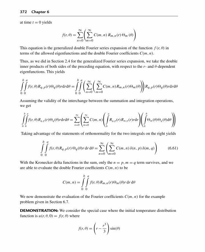
372 Chapter 6
at time t = 0 yields
f(r, θ) =∞∑
n=0
( ∞∑m=0
C(m,n)Rm,n(r)�m (θ)
)
This equation is the generalized double Fourier series expansion of the function f (r, θ) interms of the allowed eigenfunctions and the double Fourier coefficients C(m,n).
Thus, as we did in Section 2.4 for the generalized Fourier series expansion, we take the doubleinner products of both sides of the preceding equation, with respect to the r- and θ-dependenteigenfunctions. This yields
b∫0
a∫0
f(r, θ)Rq,p(r)�q(θ)rdrdθ =b∫
0
a∫0
( ∞∑n=0
( ∞∑m=0
C(m,n)Rm,n(r)�m(θ)
))Rq,p(r)�q(θ)rdrdθ
Assuming the validity of the interchange between the summation and integration operations,we get
b∫0
a∫0
f(r, θ)Rq,p(r)�q(θ)rdrdθ =∞∑
n=0
⎛⎝ ∞∑
m=0
C(m,n)
⎛⎝ a∫
0
Rq,p(r)Rm,n(r)rdr
⎞⎠⎛⎝ b∫
0
�m(θ)�q(θ)dθ
⎞⎠⎞⎠
Taking advantage of the statements of orthonormality for the two integrals on the right yields
b∫0
a∫0
f(r, θ)Rq,p(r)�q(θ)r dr dθ =∞∑
n=0
( ∞∑m=0
C(m,n) δ(n,p) δ(m,q)
)(6.61)
With the Kronecker delta functions in the sum, only the n = p,m = q term survives, and weare able to evaluate the double Fourier coefficients C(m,n) to be
C(m,n) =b∫
0
a∫0
f(r, θ)Rm,n(r)�m(θ)r dr dθ
We now demonstrate the evaluation of the Fourier coefficients C(m,n) for the exampleproblem given in Section 6.7.
DEMONSTRATION: We consider the special case where the initial temperature distributionfunction is u(r, θ,0) = f(r, θ) where
f(r, θ) =(
r − r3
3
)sin(θ)

The Diffusion Equation in Two Spatial Dimensions 373
SOLUTION: At time t = 0, the solution u(r, θ, t) reads(r − r3
3
)sin(θ) =
∞∑n=1
( ∞∑m=1
C(m,n)Rm,n(r)�m (θ)
)
where, from the preceding example, the orthonormalized eigenfunctions are
�m =√
2
πsin(mθ)
and
Rm,n(r) = J(m,λm,nr)∫ 10 J
(m,λm,nr
)2r dr
for m = 1,2,3, . . . , and n = 1,2,3, . . . . Insertion of these eigenfunctions into the series yields(r − r3
3
)sin(θ) =
∞∑n=1
( ∞∑m=1
C(m,n)Rm,n(r)
√2
πsin(mθ)
)
This is the double Fourier series expansion of f(r, θ). From the preceding, the Fouriercoefficients C(m,n) were evaluated by taking the double inner product of the initial conditionfunction f(r, θ) with respect to the corresponding orthonormal eigenfunctions. This yieldedthe integral
C(m,n) =1∫
0
π∫0
(r − r3
3
)sin(θ)Rm,n(r) r�m(θ)dθ dr
which, for the given eigenfunctions, reduces to
C(m,n) =1∫
0
π∫0
(r − r3
3
)sin(θ)Rm,n(r)r
√2
πsin(mθ)dθ dr
for m,n = 1,2,3, . . . . We integrate first with respect to θ. Since f(r, θ) depends on the termsin(mθ) for the case m = 1, then from the orthogonality condition on the θ equation, we seethat only the m = 1 solution survives here. Thus, we get
C(1, n) =1∫
0
π∫0
(r − r3
3
)sin(θ)2R1,n(r)r
√2
πdθ dr
where, for m = 1,
R1,n = J(1, λ1,nr)√∫ 10 J(1, λ2
1,nr)r dr

374 Chapter 6
Evaluation of the above for R1,n yields
R1,n = J(1, λ1,nr)√
2λ1,n√λ2
1,n−1J(1, λ1,n)
Inserting this into C(1, n) and integrating yields
C(1, n) = 8√
π
3λ31,n
√λ2
1,n−1
Thus, the final solution to the problem reads
u(r, θ, t) =∞∑
n=1
16e−λ21,n t
50 J(1, λ1,nr) sin(θ)
3λ21,n
(λ2
1,n−1
)J(1, λ1,n)
This solution is completed upon evaluation of the eigenvalues λ1,n from the eigenvalueequation
J(1, λ1,n)−λ1,n J(2, λ1,n) = 0
The details for the development of the solution and the graphics are given later in one of theMaple worksheets.
6.9 Example Diffusion Problems in Cylindrical Coordinates
We now consider several examples of partial differential equations for heat or diffusionphenomena under various homogeneous boundary conditions over finite intervals in thecylindrical coordinate system. We note that the r-dependent ordinary differential equations inthe cylindrical coordinate system are of the Bessel type and the θ-dependent ones are of theEuler type.
EXAMPLE 6.9.1: We seek the temperature distribution u(r, θ, t) in a thin circular plate overthe two-dimensional domain D = {(r, θ) |0 < r < 1,0 < θ < π/2}. The lateral surfaces of theplate are insulated. The edges r = 1 and θ = 0 are at a fixed temperature of 0, and the edgeθ = π/2 is insulated. The initial temperature distribution u(r, θ,0) = f(r, θ) is given following.The thermal diffusivity is k = 1/50.
SOLUTION: The two-dimensional homogeneous diffusion equation is
∂
∂tu(r, θ, t) = k
⎛⎜⎜⎜⎜⎝
∂
∂ru(r, θ, t)+ r
(∂2
∂r2u(r, θ, t)
)
r+
∂2
∂θ2u(r, θ, t)
r2
⎞⎟⎟⎟⎟⎠

The Diffusion Equation in Two Spatial Dimensions 375
The boundary conditions are type 1 at r = 1, type 1 at θ = 0, and type 2 at θ = π/2 and a finitesolution at the origin:
|u(0, θ, t)| < ∞ and u(1, θ, t) = 0
and
u(r,0, t) = 0 and uθ
(r,
π
2, t
)= 0
The initial condition is
u(r, θ,0) = (r − r3) sin(θ)
The ordinary differential equations from the method of separation of variables are
d
dtT(t)+kλ2 T(t) = 0
r2
(d2
dr2R(r)
)+ r
(d
drR(r)
)+ (λ2 r2 −μ2)R(r) = 0
d2
dθ2�(θ)+μ2�(θ) = 0
The boundary conditions on the spatial variables are
|R(0)| < ∞ and R(1) = 0
and
�(0) = 0 and �θ
(π
2
)= 0
Assignment of system parameters
> restart:with(plots):a:=1:b:=Pi/2:k:=1/50:
Allowed eigenvalues and corresponding orthonormal eigenfunctions are obtained fromExamples 2.5.2 and 2.6.2.
> mu[m]:=(2*m−1)*Pi/(2*b);
μm := 2m−1 (6.62)
for m = 1,2,3, . . . .
Eigenvalues λm,n are the roots of the eigenvalue equation
> BesselJ(mu[m],lambda[m,n]*a)=0;
BesselJ(2m−1, λm,n) = 0 (6.63)
for m = 1,2,3, . . . , n = 1,2,3, . . . .

376 Chapter 6
Orthonormal eigenfunctions
> R[m,n](r):=BesselJ(mu[m],lambda[m,n]*r)/sqrt(Int(BesselJ(mu[m],lambda[m,n]*r)ˆ2*r,r=0..a));R[m,p](r):=subs(n=p,R[m,n](r)):
Rm,n(r) := BesselJ(2m−1, λm,n r)√∫ 10 BesselJ(2m−1, λm,n r)2 r dr
(6.64)
> Theta[m](theta):=sqrt(2/b)*sin((2*m−1)*Pi/(2*b)*theta);Theta[q](theta):=subs(m=q,Theta[m](theta)):
�m(θ) := 2 sin((2 m−1) θ)√π
(6.65)
Statements of orthonormality with their respective weight functions
> w(r):=r:Int(R[m,n](r)*R[m,p](r)*w(r),r=0...a)=delta(n,p);
1∫0
BesselJ(2m−1, λm,nr) BesselJ(2m−1, λm,pr)r√∫ 10 BesselJ(2m−1, λm,nr)2 r dr
√∫ 10 BesselJ(2m−1, λm,pr)2 r dr
dr = δ(n,p) (6.66)
> w(theta):=1:Int(Theta[m](theta)*Theta[q](theta)*w(theta),theta=0...b)=delta(m,q);
12 π∫0
4 sin((2m−1)θ) sin((2q−1)θ)
πdθ = δ(m,q) (6.67)
Time-dependent solution
> T[m,n](t):=C(m,n)*exp(−k*lambda[m,n]ˆ2*t);
Tm,n(t) := C(m,n) e− 150 λ2
m,n t (6.68)
Generalized series terms
> u[m,n](r,theta,t):=T[m,n](t)*R[m,n](r)*Theta[m](theta);
um,n(r, θ, t) := 2C(m,n)e− 150 λ2
m,n t BesselJ(2m−1, λm,nr) sin((2m−1)θ)√∫ 10 BesselJ(2m−1, λm,nr)2r dr
√π
(6.69)
Eigenfunction expansion
> u(r,theta,t):=Sum(Sum(u[m,n](r,theta,t),m=1..infinity),n=1..infinity);
u(r, θ, t) :=∞∑
n=1
⎛⎜⎝ ∞∑
m=1
2C(m,n)e− 150 λ2
m,n t BesselJ(2m−1, λm,nr) sin((2m−1)θ)√∫ 10 BesselJ(2m−1, λm,nr)2 r dr
√π
⎞⎟⎠ (6.70)

The Diffusion Equation in Two Spatial Dimensions 377
The Fourier coefficients C(m,n) are to be determined from the initial condition functionu(r, θ,0) = f(r, θ). We consider the special case where
> f(r,theta):=(r−rˆ3)*sin(theta);
f(r, θ) := (r − r3) sin(θ) (6.71)
At time t = 0, we have
> f(r,theta)=eval(subs(t=0,u(r,theta,t)));
(r − r3) sin(θ) =∞∑
n=1
⎛⎜⎝ ∞∑
m=1
2C(m,n) BesselJ(2m−1, λm,n r) sin((2m−1)θ)√∫ 10 BesselJ(2m−1, λm,n r))2r dr
√π
⎞⎟⎠ (6.72)
This is the double Fourier series expansion of f(r, θ). From Section 6.8, the Fourier coefficientsC(m,n) were evaluated by taking the double inner product of the initial condition functionf(r, θ) with respect to the corresponding orthonormalized eigenfunctions given earlier.
Because f(r, θ) depends on sin((2m−1)θ) for the case for m = 1, then, from the precedingorthogonality statement for θ, only the m = 1 solution survives here, and we set
> Theta[1](theta):=subs(m=1,eval(Theta[m](theta)));
�1(θ) := 2 sin(θ)√π
(6.73)
Eigenvalues λ1,n are the roots of the eigenvalue equation
> subs({m=1,r=a},BesselJ(mu[m],lambda[m,n]*r))=0;
BesselJ(1, λ1,n) = 0 (6.74)
Evaluation of the orthonormalized eigenfunctions for m = 1 yields
> R[1,n](r):=eval(subs(m=1,BesselJ(mu[m],lambda[m,n]*r)/sqrt(expand(int(subs(m=1,BesselJ(mu[m],lambda[m,n]*r))ˆ2*r,r=0..a)))));
R1,n(r) := 2 BesselJ(1, λ1,n r)√2 BesselJ(0, λ1,n)2 − 4 BesselJ(0, λ1,n) BesselJ(1, λ1,n)
λ1,n+2 BesselJ(1, λ1,n)2
(6.75)
Substitution of the preceding eigenvalue equation simplifies this
> R[1,n](r):=radsimp(subs(BesselJ(1,lambda[1,n]*a)=0,R[1,n](r)));
R1,n(r) := BesselJ(1, λ1,n r)√
2
BesselJ(0, λ1,n)(6.76)

378 Chapter 6
Evaluation of the Fourier coefficients yields
> C(1,n):=Int(Int(f(r,theta)*R[1,n](r)*w(r)*Theta[1](theta)*w(theta),r=0..a),theta=0..b);
C(1, n) :=12 π∫0
1∫0
2(r − r3) sin(θ)2 BesselJ(1, λ1,nr)√
2 r
BesselJ(0, λ1,n)√
πdr dθ (6.77)
> C(1,n):=radsimp(subs(BesselJ(1,lambda[1,n]*a)=0,value(%)));
C(1, n) := −4√
2√
π
λ31,n
(6.78)
> T[1,n](t):=eval(subs(m=1,T[m,n](t)));
T1,n(t) := −4√
2√
π e− 150 λ2
1,nt
λ31,n
(6.79)
Generalized series terms
> u[1,n](r,theta,t):=(T[1,n](t)*R[1,n](r)*Theta[1](theta));
u1,n(r, θ, t) := −16 e− 150 λ2
1,n t BesselJ(1, λ1,n r) sin(θ)
λ31,n
BesselJ(0, λ1,n)(6.80)
Series solution
> u(r,theta,t):=Sum(u[1,n](r,theta,t),n=1..infinity);
u(r, θ, t) :=∞∑
n=1
⎛⎝−16 e− 1
50 λ21,n t BesselJ(1, λ1,n r) sin(θ)
λ31,n
BesselJ(0, λ1,n)
⎞⎠ (6.81)
Evaluation of the eigenvalues λ1,n from the roots of the eigenvalue equation yields
> subs({m=1,r=a},BesselJ(mu[m],lambda[m,n]*r))=0;
BesselJ(1, λ1,n) = 0 (6.82)
> plot(BesselJ(1,v),v=0..20,thickness=10);
If we set v = λa, then the eigenvalues λ1,n are found from the intersection points of the curveof J(1, v) with the v-axis shown in Figure 6.9. Using the Maple fsolve command to evaluatethe first few eigenvalues yields
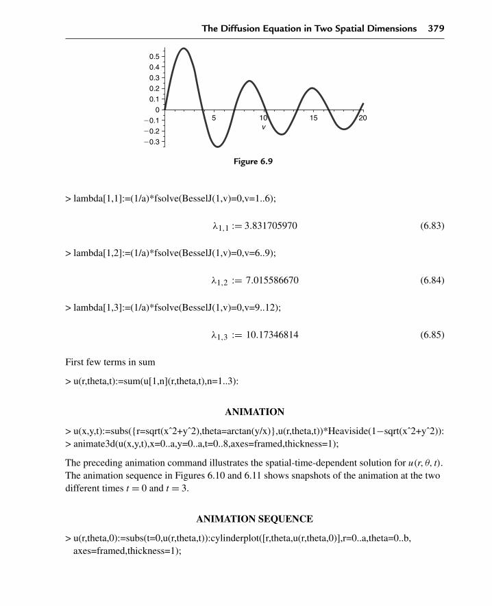
The Diffusion Equation in Two Spatial Dimensions 379
5
0.5
0.4
0.3
0.2
0.1
20.1
20.2
20.3
010v
15 20
Figure 6.9
> lambda[1,1]:=(1/a)*fsolve(BesselJ(1,v)=0,v=1..6);
λ1,1 := 3.831705970 (6.83)
> lambda[1,2]:=(1/a)*fsolve(BesselJ(1,v)=0,v=6..9);
λ1,2 := 7.015586670 (6.84)
> lambda[1,3]:=(1/a)*fsolve(BesselJ(1,v)=0,v=9..12);
λ1,3 := 10.17346814 (6.85)
First few terms in sum
> u(r,theta,t):=sum(u[1,n](r,theta,t),n=1..3):
ANIMATION
> u(x,y,t):=subs({r=sqrt(xˆ2+yˆ2),theta=arctan(y/x)},u(r,theta,t))*Heaviside(1−sqrt(xˆ2+yˆ2)):> animate3d(u(x,y,t),x=0..a,y=0..a,t=0..8,axes=framed,thickness=1);
The preceding animation command illustrates the spatial-time-dependent solution for u(r, θ, t).The animation sequence in Figures 6.10 and 6.11 shows snapshots of the animation at the twodifferent times t = 0 and t = 3.
ANIMATION SEQUENCE
> u(r,theta,0):=subs(t=0,u(r,theta,t)):cylinderplot([r,theta,u(r,theta,0)],r=0..a,theta=0..b,axes=framed,thickness=1);

380 Chapter 6
0.30.20.1
00
0.20.4
0.60.8 0.8
0.60.4
0.20
1 1
z
y x
Figure 6.10
> u(r,theta,3):=subs(t=3,u(r,theta,t)):cylinderplot([r,theta,u(r,theta,3)],r=0..a,theta=0..b,axes=framed,thickness=1);
0.160.120.080.04
00
0.20.4
0.60.8 0.8
0.60.4
0.20
1 1
z
y x
Figure 6.11
EXAMPLE 6.9.2: We seek the temperature distribution in a thin circular plate over thetwo-dimensional domain D = {(r, θ) |0 < r < 1,0 < θ < π}. The lateral surfaces of the plateare insulated. The sides θ = 0 and θ = π are at a fixed temperature of 0, and the edge r = 1 isinsulated. The initial temperature distribution u(r, θ,0) = f(r, θ) is given as follows, and thethermal diffusivity is k = 1/25.
SOLUTION: The two-dimensional homogeneous diffusion equation is
∂
∂tu(r, θ, t) = k
⎛⎝ ∂
∂r u(r, θ, t)+ r(
∂2
∂r2 u(r, θ, t))
r+
∂2
∂θ2 u(r, θ, t)
r2
⎞⎠
The boundary conditions are type 2 at r = 1, type 1 at θ = 0, and type 1 at θ = π and a finitesolution at the origin:
|u(0, θ, t)| < ∞ and ur(1, θ, t) = 0
and
u(r,0, t) = 0 and u(r,π, t) = 0

The Diffusion Equation in Two Spatial Dimensions 381
The initial condition is
u(r, θ,0) =(
r − r3
3
)sin(θ)
The ordinary differential equations from the method of separation of variables are
d
dtT(t)+kλ2T(t) = 0
r2
(d2
dr2R(r)
)+ r
(d
drR(r)
)+
(λ2r2 −μ2
)R(r) = 0
d2
dθ2�(θ)+μ2�(θ) = 0
The boundary conditions on the spatial variables are
|R(0)| < ∞ and Rr(1) = 0
and
�(0) = 0 and �(π) = 0
Assignment of system parameters
> restart:with(plots):a:=1:b:=Pi:k:=1/25:
Allowed eigenvalues and corresponding orthonormal eigenfunctions are obtained fromExamples 2.5.1 and 2.6.3.
> mu[m]:=m*Pi/b;
μm := m (6.86)
for m = 1,2,3, . . . .
Eigenvalues λm,n are the roots of the eigenvalue equation
> subs(r=a,diff(BesselJ(mu[m],lambda[m,n]*r),r))=0;
(−BesselJ(m+1, λm,n)+ mBesselJ(m,λm,n)
λm,n
)λm,n = 0 (6.87)
for m = 1,2,3, . . . , n = 1,2,3, . . . .

382 Chapter 6
Orthonormal eigenfunctions
> R[m,n](r):=BesselJ(mu[m],lambda[m,n]*r)/sqrt(Int(BesselJ(mu[m],lambda[m,n]*r)ˆ2*r,r=0..a));R[m,p](r):=subs(n=p,R[m,n](r)):
Rm,n(r) := BesselJ(m,λm,nr)√1∫0
BesselJ(m,λm,nr)2r dr
(6.88)
> Theta[m](theta):=sqrt(2/b)*sin(m*Pi/b*theta);Theta[q](theta):=subs(m=q,Theta[m](theta)):
�m(θ) :=√
2 sin(mθ)√π
(6.89)
Statements of orthonormality with their respective weight functions
> w(r):=r:Int(R[m,n](r)*R[m,p](r)*w(r),r=0...a)=delta(n,p);
1∫0
BesselJ(m,λm,nr)BesselJ(m,λm,pr)r√1∫0
BesselJ(m,λm,nr)2r dr
√1∫0
BesselJ(m,λm,pr)2r dr
dr = δ(n,p) (6.90)
> w(theta):=1:Int(Theta[m](theta)*Theta[q](theta)*w(theta),theta=0...b)=delta(m,q);
π∫0
2 sin(mθ) sin(qθ)
πdθ = δ(m,q) (6.91)
Time-dependent solution
> T[m,n](t):=C(m,n)*exp(−k*lambda[m,n]ˆ2*t);
Tm,n(t) := C(m,n) e− 125λ2
m,nt (6.92)
Generalized series terms
> u[m,n](r,theta,t):=T[m,n](t)*R[m,n](r)*Theta[m](theta);
um,n(r, θ, t) := C(m,n)e− 125λ2
m,nt BesselJ(m,λm,nr)√
2 sin(mθ)√∫ 10 BesselJ(m,λm,nr)2r dr
√π
(6.93)

The Diffusion Equation in Two Spatial Dimensions 383
Eigenfunction expansion
> u(r,theta,t):=Sum(Sum(u[m,n](r,theta,t),m=0..infinity),n=0..infinity);
u(r, θ, t) :=∞∑
n=0
⎛⎜⎝ ∞∑
m=0
C(m,n)e− 125λ2
m,nt BesselJ(m,λm,nr)√
2 sin(mθ)√∫ 10 BesselJ(m,λm,nr)2r dr
√π
⎞⎟⎠ (6.94)
The Fourier coefficients C(m,n) are to be determined from the initial condition functionu(r, θ,0) = f(r, θ). We consider the special case where
> f(r,theta):=(r−rˆ3/3)*sin(theta);
f(r, θ) :=(
r − 1
3r3
)sin(θ) (6.95)
At time t = 0, we have
> f(r,theta)=eval(subs(t=0,u(r,theta,t)));
(r − 1
3r3
)sin(θ) =
∞∑n=0
⎛⎜⎝ ∞∑
m=0
C(m,n)BesselJ(m,λm,nr)√
2 sin(mθ)√∫ 10 BesselJ(m,λm,nr)2 rdr
√π
⎞⎟⎠ (6.96)
This is the double Fourier series expansion of f(r, θ). From Section 6.8, the Fourier coefficientsC (m,n) were evaluated by taking the double inner product of the initial condition functionf(r, θ) with respect to the preceding corresponding orthonormalized eigenfunctions.
Because f(r, θ) depends on sin(mθ) for the m = 1 case, then, from the given orthogonalitystatement for θ, only the m = 1 solution survives here, and we set
> Theta[1](theta):=subs(m=1,eval(Theta[m](theta)));
�1(θ) :=√
2 sin(θ)√π
(6.97)
Eigenvalues λ1,n are the roots of the eigenvalue equation
> subs({m=1,r=a},diff(BesselJ(mu[m],lambda[m,n]*r),r))=0;(−BesselJ(2, λ1,n)+ BesselJ(1, λ1,n)
λ1,n
)λ1,n = 0 (6.98)
For m = 1, we have the Bessel identity
> subs(m=1,BesselJ(m−1,lambda[m,n]*a)=2*m*BesselJ(m,lambda[m,n]*a)/(lambda[m,n]*a)−BesselJ(m+1,lambda[m,n]*a));
BesselJ(0, λ1,n) = 2BesselJ(1, λ1,n)
λ1,n−BesselJ(2, λ1,n) (6.99)

384 Chapter 6
Evaluation of the orthonormalized eigenfunctions for m= 1
> R[1,n](r):=eval(subs(m=1,BesselJ(mu[m],lambda[m,n]*r)/sqrt(expand(int(subs(m=1,BesselJ(mu[m],lambda[m,n]*r))ˆ2*r,r=0..a)))));
R1,n(r) := 2BesselJ(1, λ1,nr)√2 BesselJ(0, λ1,n)2 − 4 BesselJ(0, λ1,n) BesselJ(1, λ1,n)
λ1,n+2 BesselJ(1, λ1,n)2
(6.100)
Substitution of the preceding eigenvalue equation and the Bessel identity simplifies this to
> R[1,n](r):=radsimp(subs(BesselJ(0,lambda[1,n]*a)=BesselJ(1,lambda[1,n]*a)/(lambda[1,n]*a),R[1,n](r)));
R1,n(r) := BesselJ(1, λ1,nr)√
2λ1,n
BesselJ(1, λ1,n)
√−1+λ2
1,n
(6.101)
Evaluation of the Fourier coefficients yields
> C(1,n):=Int(Int(f(r,theta)*R[1,n](r)*w(r)*Theta[1](theta)*w(theta),r=0..a),theta=0..b);
C(1, n) :=π∫
0
1∫0
2(r − 1
3r3)
sin(θ)2BesselJ(1, λ1,nr)λ1,nr
BesselJ(1, λ1,n)
√−1+λ2
1,n
√π
dr dθ (6.102)
> C(1,n):=simplify(subs(BesselJ(0,lambda[1,n]*a)=BesselJ(1,lambda[1,n]*a)/(lambda[1,n]*a),value(%)));
C(1, n) := 8
3
√π
λ31,n
√−1+λ2
1,n
(6.103)
> T[1,n](t):=eval(subs(m=1,T[m,n](t)));
T1,n(t) := 8
3
√π e− 1
25λ21,nt
λ31,n
√−1+λ2
1,n
(6.104)
Generalized series terms
> u[1,n](r,theta,t):=T[1,n](t)*R[1,n](r)*Theta[1](theta);
u1,n(r, θ, t) := 16
3
e− 125λ2
1,ntBesselJ(1, λ1,nr) sin(θ)
λ21,n
(−1+λ2
1,n
)BesselJ(1, λ1,n)
(6.105)
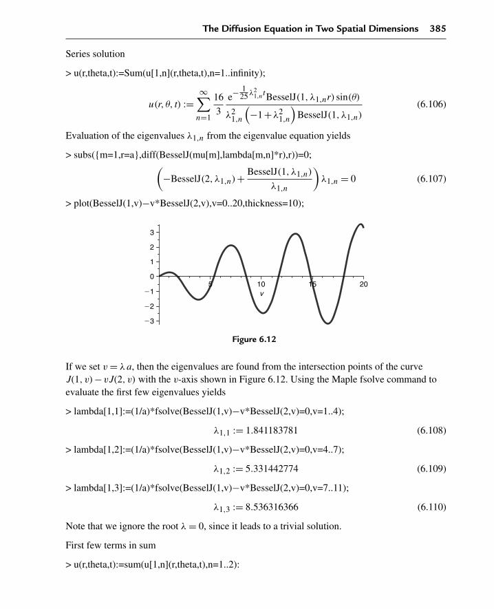
The Diffusion Equation in Two Spatial Dimensions 385
Series solution
> u(r,theta,t):=Sum(u[1,n](r,theta,t),n=1..infinity);
u(r, θ, t) :=∞∑
n=1
16
3
e− 125λ2
1,ntBesselJ(1, λ1,nr) sin(θ)
λ21,n
(−1+λ2
1,n
)BesselJ(1, λ1,n)
(6.106)
Evaluation of the eigenvalues λ1,n from the eigenvalue equation yields
> subs({m=1,r=a},diff(BesselJ(mu[m],lambda[m,n]*r),r))=0;(−BesselJ(2, λ1,n)+ BesselJ(1, λ1,n)
λ1,n
)λ1,n = 0 (6.107)
> plot(BesselJ(1,v)−v*BesselJ(2,v),v=0..20,thickness=10);
5
3
2
1
21
22
23
010v
15 20
Figure 6.12
If we set v = λa, then the eigenvalues are found from the intersection points of the curveJ(1, v)−vJ(2, v) with the v-axis shown in Figure 6.12. Using the Maple fsolve command toevaluate the first few eigenvalues yields
> lambda[1,1]:=(1/a)*fsolve(BesselJ(1,v)−v*BesselJ(2,v)=0,v=1..4);
λ1,1 := 1.841183781 (6.108)
> lambda[1,2]:=(1/a)*fsolve(BesselJ(1,v)−v*BesselJ(2,v)=0,v=4..7);
λ1,2 := 5.331442774 (6.109)
> lambda[1,3]:=(1/a)*fsolve(BesselJ(1,v)−v*BesselJ(2,v)=0,v=7..11);
λ1,3 := 8.536316366 (6.110)
Note that we ignore the root λ = 0, since it leads to a trivial solution.
First few terms in sum
> u(r,theta,t):=sum(u[1,n](r,theta,t),n=1..2):
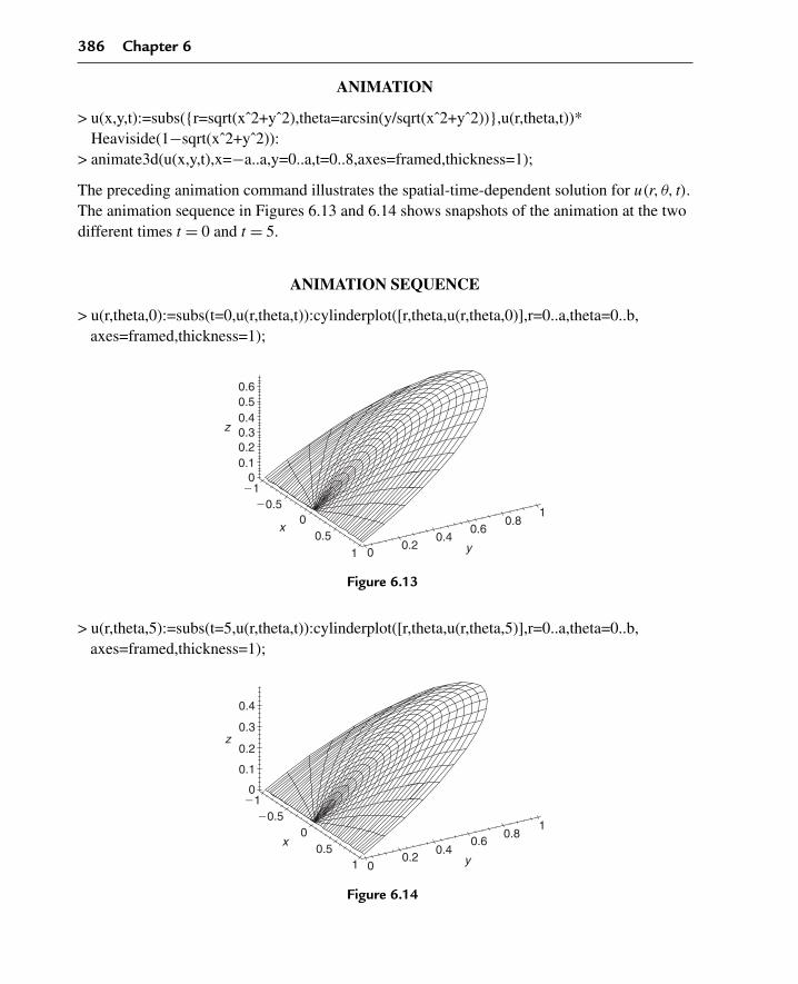
386 Chapter 6
ANIMATION
> u(x,y,t):=subs({r=sqrt(xˆ2+yˆ2),theta=arcsin(y/sqrt(xˆ2+yˆ2))},u(r,theta,t))*Heaviside(1−sqrt(xˆ2+yˆ2)):
> animate3d(u(x,y,t),x=−a..a,y=0..a,t=0..8,axes=framed,thickness=1);
The preceding animation command illustrates the spatial-time-dependent solution for u(r, θ, t).The animation sequence in Figures 6.13 and 6.14 shows snapshots of the animation at the twodifferent times t = 0 and t = 5.
ANIMATION SEQUENCE
> u(r,theta,0):=subs(t=0,u(r,theta,t)):cylinderplot([r,theta,u(r,theta,0)],r=0..a,theta=0..b,axes=framed,thickness=1);
0.6
0.6
y
x 0.81
0.50.4
0.4
0.30.2
0.2
0.10
2120.5
0
00.5
1
z
Figure 6.13
> u(r,theta,5):=subs(t=5,u(r,theta,t)):cylinderplot([r,theta,u(r,theta,5)],r=0..a,theta=0..b,axes=framed,thickness=1);
0.6
y
x0.8
1
0.4
0.4
0.3
0.2
0.2
0.1
021
20.50
00.5
1
z
Figure 6.14

The Diffusion Equation in Two Spatial Dimensions 387
EXAMPLE 6.9.3: We consider the temperature distribution in a thin circular plate over thetwo-dimensional domain D = {(r, θ) |0 < r < 1,−π < θ < π}. The lateral surfaces of the plateare insulated. The periphery r = 1 is held at a fixed temperature of 0, and the θ-dependentsolution satisfies periodic boundary conditions. The initial temperature distributionu(r, θ,0) = f(r, θ) is given as follows, and the thermal diffusivity is k = 1/50.
SOLUTION: The two-dimensional homogeneous diffusion equation is
∂
∂tu(r, θ, t) = k
⎛⎝ ∂
∂r u(r, θ, t)+ r(
∂2
∂r2 u(r, θ, t))
r+
∂2
∂θ2 u(r, θ, t)
r2
⎞⎠
The boundary conditions are type 1 at r = 1, a finite solution at the origin, and periodicboundary conditions on θ:
|u(0, θ, t)| < ∞ and u(1, θ, t) = 0
and
u(r,−π, t) = u(r,π, t) and uθ(r,−π, t) = uθ(r,π, t)
The initial condition is
u(r, θ,0) =(r2 − r4
)sin(2 θ)
The ordinary differential equations from the method of separation of variables are
d
dtT(t)+kλ2T(t) = 0
r2
(d2
dr2R(r)
)+ r
(d
drR(r)
)+
(λ2r2 −μ2
)R(r) = 0
d2
dθ2�(θ)+μ2�(θ) = 0
The boundary conditions on the spatial variables are
|R(0)| < ∞ and R(1) = 0
and
�(−π) = �(π) and �θ(−π) = �θ(π)
Assignment of system parameters
> restart:with(plots):a:=1:b:=Pi:k:=1/50:
Allowed eigenvalues and corresponding orthonormal eigenfunctions are obtained fromExamples 2.6.1 and 2.6.2.
388 Chapter 6
> mu[m]:=m*Pi/b;
μm := m (6.111)
for m = 1,2,3, . . . .
Eigenvalues λm,n are the roots of the eigenvalue equation
> BesselJ(mu[m],lambda[m,n]*a)=0;
BesselJ(m,λm,n) = 0 (6.112)
for m = 1,2,3, . . . , n = 1,2,3, . . . .
Orthonormal eigenfunctions
> R[m,n](r):=BesselJ(mu[m],lambda[m,n]*r)/sqrt(Int(BesselJ(mu[m],lambda[m,n]*r)ˆ2*r,r=0..a));R[m,p](r):=subs(n=p,R[m,n](r)):
Rm,n(r) := BesselJ(m,λm,nr)√∫ 10 BesselJ(m,λm,nr)2r dr
(6.113)
> phi[m](theta):=sqrt(1/Pi)*cos(m*theta);phi[q](theta):=subs(m=q,phi[m](theta)):
φm(θ) := cos(mθ)√π
(6.114)
> psi[m](theta):=sqrt(1/Pi)*sin(m*theta);psi[q](theta):=subs(m=q,psi[m](theta)):
�m(θ) := sin(mθ)√π
(6.115)
For m = 0, the eigenvalues are the roots of the equation
> BesselJ(0,lambda[0,n]*a)=0;
BesselJ(0, λ0,n) = 0 (6.116)
Orthonormal eigenfunctions
> R[0,n](r):=BesselJ(0,lambda[0,n]*r)/sqrt(Int(BesselJ(0,lambda[0,n]*r)ˆ2*r,r=0..a));R[0,p](r):=subs(n=p,R[0,n](r)):
R0,n(r) := BesselJ(0, λ0,nr)√∫ 10 BesselJ(0, λ0,nr)2r dr
(6.117)
> phi[0](theta):=1/sqrt(2*Pi);
φ0(θ) := 1
2
√2√π
(6.118)

The Diffusion Equation in Two Spatial Dimensions 389
Statements of orthonormality with their respective weight functions
> w(r):=r:Int(R[m,n](r)*R[m,p](r)*w(r),r=0..a)=delta(n,p);
1∫0
BesselJ(m,λm,nr)BesselJ(m,λm,pr)r√∫ 10 BesselJ(m,λm,nr)2r dr
√∫ 10 BesselJ(m,λm,pr)2r dr
dr = δ(n,p) (6.119)
> w(theta):=1:Int(phi[m](theta)*phi[q](theta)*w(theta),theta=−Pi..Pi)=delta(m,q);
π∫−π
cos(mθ) cos(qθ)
πdθ = δ(m,q) (6.120)
> w(theta):=1:Int(psi[m](theta)*psi[q](theta)*w(theta),theta=−Pi..Pi)=delta(m,q);
π∫−π
sin(mθ) sin(qθ)
πdθ = δ(m,q) (6.121)
Time-dependent solution
> T[m,n](t):=exp(−k*lambda[m,n]ˆ2*t);u[m,n](r,theta,t):=T[m,n](t)*R[m,n](r)*(A(m,n)*phi[m](theta)+B(m,n)*psi[m](theta)):
Tm,n(t) := e− 150λ2
m,nt (6.122)
> T[0,n](t):=A(0,n)*exp(−k*lambda[0,n]ˆ2*t);u[0,n](r,theta,t):=T[0,n](t)*R[0,n](r)*phi[0](theta):
T0,n(t) := A(0, n)e− 150λ2
0,nt (6.123)
Eigenfunction expansion
> u(r,theta,t):=Sum(u[0,n](r,theta,t),n=1..infinity)+Sum(Sum(u[m,n](r,theta,t),m=1..infinity),n=1..infinity);
u(r, θ, t) : =∞∑
n=1
1
2
A(0, n)e− 150λ2
0,ntBesselJ(0, λ0,nr)√
2√∫ 10 BesselJ(0, λ0,nr)2rdr
√π
+∞∑
n=1
⎛⎜⎝ ∞∑
m=1
e− 150λ2
m,ntBesselJ(m,λm,nr)(
A(m,n) cos(mθ)√π
+ B(m,n) sin(mθ)√π
)√∫ 1
0 BesselJ(m,λm,nr)2r dr
⎞⎟⎠
(6.124)

390 Chapter 6
The Fourier coefficients A(m,n) and B(m,n) are to be determined from the initial conditionfunction u(r, θ,0) = f(r, θ). We consider the special case where
> f(r,theta):=(rˆ2−rˆ4)*sin(2*theta);
f(r, θ) :=(r2 − r4
)sin(2θ) (6.125)
At time t = 0 we have
> f(r,theta)=eval(subs(t=0,u(r,theta,t)));
(r2 − r4
)sin(2 θ) =
∞∑n=1
1
2
A(0, n)BesselJ(0, λ0,nr)√
2√∫ 10 BesselJ(0, λ0,nr)2r dr
√π
+∞∑
n=1
⎛⎜⎜⎝
∞∑m=1
BesselJ(m,λm,nr)
(A(m,n) cos(mθ)√
π+ B(m,n) sin(mθ)√
π
)√∫ 1
0 BesselJ(m,λm,nr)2r dr
⎞⎟⎟⎠
(6.126)
This is the double Fourier series expansion of f(r, θ). From Section 6.8, the Fourier coefficientsA(m,n) and B(m,n) are to be evaluated by taking the double inner product of the initialcondition function f(r, θ) with respect to the corresponding orthonormal eigenfunctions givenearlier.
Because f(r, θ) depends on sin(mθ) for the case m = 2, then, from the given orthogonalitystatement for θ, only the m = 2 solution survives here, and we set
> phi[2](theta):=subs(m=2,eval(phi[m](theta)));
φ2(θ) := cos(2θ)√π
(6.127)
> psi[2](theta):=subs(m=2,eval(psi[m](theta)));
ψ2(θ) := sin(2θ)√π
(6.128)
Eigenvalues λ2,n are the roots of the eigenvalue equation
> subs({m=2,r=a},BesselJ(mu[m],lambda[m,n]*r)=0);
BesselJ(2, λ2,n) = 0 (6.129)

The Diffusion Equation in Two Spatial Dimensions 391
For m = 2, we have the Bessel identity
> subs(m=2,BesselJ(0,lambda[m,n]*a)=2*BesselJ(1,lambda[m,n]*a)/(lambda[m,n]*a)−BesselJ(2,lambda[m,n]*a));
BesselJ(0, λ2,n) = 2BesselJ(1, λ2,n)
λ2,n−BesselJ(2, λ2,n) (6.130)
Evaluation of the normalized eigenfunctions for m = 2 yields
> R[2,n](r):=eval(subs(m=2,BesselJ(mu[m],lambda[m,n]*r)/sqrt(expand(int(subs(m=2,BesselJ(mu[m],lambda[m,n]*r))ˆ2*r,r=0..a)))));
R2,n(r) := 2BesselJ(2, λ2,nr)√√√√2BesselJ(0, λ2,n)2 +2BesselJ(1, λ2,n)2 − 8BesselJ(1, λ2,n)2
λ22,n
(6.131)
Substitution of the preceding eigenvalue equation and the Bessel identity simplifies this to
> R[2,n](r):=radsimp(subs(BesselJ(0,lambda[2,n]*a)=2*BesselJ(1,lambda[2,n]*a)/(lambda[2,n]*a),R[2,n](r)));
R2,n(r) := BesselJ(2, λ2,nr)√
2
BesselJ(1, λ2,n)(6.132)
Evaluation of the Fourier coefficients yields
> A(2,n):=Int(Int(f(r,theta)*R[2,n](r)*w(r)*phi[2](theta)*w(theta),r=0..a),theta=−Pi..Pi);
A(2, n) :=π∫
−π
1∫0
(r2 − r4
)sin(2 θ) BesselJ(2, λ2,nr)
√(2)r cos(2 θ)
BesselJ(1, λ2,n)√
πdr dθ (6.133)
> A(2,n):=value(%);
A(2, n) := 0 (6.134)
> A(0,n):=Int(Int(f(r,theta)*R[0,n](r)*w(r)*phi[0](theta)*w(theta),theta=−Pi..Pi),r=0..a);
A(0, n) :=1∫
0
π∫−π
1
2
(r2 − r4
)sin(2θ) BesselJ(0, λ0,nr)r
√2√∫ 1
0 BesselJ(0, λ0,nr)2r dr√
π
dθ dr (6.135)
> A(0,n):=value(%);
A(0, n) := 0 (6.136)

392 Chapter 6
> B(2,n):=Int(Int(f(r,theta)*R[2,n](r)*w(r)*psi[2](theta)*w(theta),r=0..a),theta=−Pi..Pi);
B(2, n) :=π∫
−π
1∫0
(r2 − r4
)sin(2θ)2 BesselJ(2, λ2,nr)
√2r
BesselJ(1, λ2,n)√
πdr dθ (6.137)
> B(2,n):=subs(BesselJ(0,lambda[2,n]*a)=2*BesselJ(1,lambda[2,n]*a)/(lambda[2,n]*a),value(%));
B(2, n) := −12√
2√
π
λ32,n
(6.138)
> T[2,n](t):=eval(subs(m=2,T[m,n](t)));
T2,n(t) := e− 150 λ2
2,nt (6.139)
Generalized series terms
> u[2,n](r,theta,t):=(T[2,n](t)*R[2,n](r)*(A(2,n)*phi[2](theta)+B(2,n)*psi[2](theta)));
u2,n(r, θ, t) := −24 e− 150λ2
2,nt BesselJ(2, λ2,nr) sin(2θ)
BesselJ(1, λ2,n)λ32,n
(6.140)
> T[0,n]:=eval(T[0,n](t));u[0,n](r,theta,t):=T[0,n](t)*R[0,n](r)*phi[0](theta):
T0,n := 0 (6.141)
Series solution
> u(r,theta,t):=Sum(u[2,n](r,theta,t),n=1..infinity);
u(r, θ, t) :=∞∑
n=1
⎛⎝−24 e− 1
50λ22,nt BesselJ(2, λ2,nr) sin(2θ)
BesselJ(1, λ2,n)λ32,n
⎞⎠ (6.142)
Evaluation of the eigenvalues λ2,n from the roots of the eigenvalue equation yields
> subs({r=a,m=2},BesselJ(mu[m],lambda[m,n]*r))=0;
BesselJ(2, λ2,n) = 0 (6.143)
> plot(BesselJ(2,v),v=0..20,thickness=10);
If we set v = λa, then the eigenvalues are found from the intersection points of the curveJ(2, v) with the v-axis shown in Figure 6.15. A few of these eigenvalues using the Maple fsolvecommand yields

The Diffusion Equation in Two Spatial Dimensions 393
5
0.4
0.3
0.2
0.1
20.1
20.2
20.3
010v
15 20
Figure 6.15
> lambda[2,1]:=(1/a)*fsolve(BesselJ(2,v)=0,v=1..6);
λ2,1 := 5.135622302 (6.144)
> lambda[2,2]:=(1/a)*fsolve(BesselJ(2,v)=0,v=6..10);
λ2,2 := 8.417244140 (6.145)
> lambda[2,3]:=(1/a)*fsolve(BesselJ(2,v)=0,v=10..14);
λ2,3 := 11.61984117 (6.146)
First few terms of sum
> u(r,theta,t):=sum(u[2,n](r,theta,t),n=1..1):
ANIMATION
> u(x,y,t):=subs({r=sqrt(xˆ2+yˆ2),theta=arctan(y/x)},u(r,theta,t))*Heaviside(1−sqrt(xˆ2+yˆ2)):> animate3d(u(x,y,t),x=−a..a,y=−a..a,t=0..5,axes=framed,thickness=1);
ANIMATION SEQUENCE
The preceding animation illustrates the spatial-time-dependent solution for u(r, θ, t). Theanimation sequence in Figures 6.16 and 6.17 shows snapshots of the animation at the twodifferent times t = 0 and t = 4.
> u(r,theta,0):=subs(t=0,u(r,theta,t)):cylinderplot([r,theta,u(r,theta,0)],r=0..a,theta=−Pi..Pi,axes=framed,thickness=1);

394 Chapter 6
0.20.1
020.1
2120.5
2120.5
00.5
20.2
0.50
1 1
z
y x
Figure 6.16
> u(r,theta,4):=subs(t=4,u(r,theta,t)):cylinderplot([r,theta,u(r,theta,4)],r=0..a,theta=−Pi..Pi,axes=framed,thickness=1);
0.020.03
0.010
20.0120.0220.03
z
2120.5
2120.5
00.5 0.5
0
1 1y x
Figure 6.17
Chapter Summary
Nonhomogeneous diffusion equation in two dimensions in rectangular coordinates
∂
∂tu(x, y, t) = k
(∂2
∂x2u(x, y, t)+ ∂2
∂y2u(x, y, t)
)+h(x, y, t)
Linear diffusion operator in two dimensions in rectangular coordinates
L(u) = ∂
∂tu(x, y, t)−k
(∂2
∂x2u(x, y, t)+ ∂2
∂y2u(x, y, t)
)
Method of separation of variables solution
u(x, y, t) = X(x)Y(y)T(t)

The Diffusion Equation in Two Spatial Dimensions 395
Eigenfunction expansion solution for rectangular coordinates
u(x, y, t) =∞∑
n=0
( ∞∑m=0
Xm(x)Yn(y)C(m,n)e−kλm,nt
)
Initial condition Fourier coefficients for rectangular coordinates
C(m,n) =b∫
0
a∫0
f(x, y)Xm(x)Yn(y)dxdy
Nonhomogeneous diffusion equation in two dimensions in cylindrical coordinates
∂
∂tu(r, θ, t) = k
⎛⎝ ∂
∂r u(r, θ, t)+ r(
∂2
∂r2 u(r, θ, t))
r+
∂2
∂θ2 u(r, θ, t)
r2
⎞⎠+h(r, θ, t)
Linear diffusion operator in two dimensions in cylindrical coordinates
L(u) = ∂
∂tu(r, θ, t)−k
⎛⎝ ∂
∂r u(r, θ, t)+ r(
∂2
∂r2 u(r, θ, t))
r+
∂2
∂θ2 u(r, θ, t)
r2
⎞⎠
Method of separation of variables solution
u(r, θ, t) = R(r)�(θ)T(t)
Eigenfunction expansion solution in cylindrical coordinates
u(r, θ, t) =∞∑
n=0
( ∞∑m=0
Rm,n(r)�m(θ)C(m,n)e−kλ2m,nt
)
Initial condition Fourier coefficients for cylindrical coordinates
C(m,n) =b∫
0
a∫0
f(r, θ)Rm,n(r)�m(θ)rdr dθ
We have examined homogeneous partial differential equations describing diffusion phenomenain two spatial dimensions for both the rectangular and the cylindrical coordinate systems.
Exercises
We now consider diffusion or heat equations with homogeneous boundary conditions in twodimensions in both the rectangular coordinate and cylindrical coordinate systems. We use themethod of separation of variables and eigenfunction expansions to evaluate the solutions.
396 Chapter 6
Two Dimensions, Rectangular Coordinates
We seek the temperature distribution in thin plates over the two-dimensional domainD = {(x, y) |0 < x < 1,0 < y < 1} whose lateral surfaces are insulated. The two-dimensionalhomogeneous partial differential equation in rectangular coordinates reads
∂
∂tu(x, y, t) = k
(∂2
∂x2u(x, y, t)+ ∂2
∂y2u(x, y, t)
)
For Exercises 6.1 through 6.25, the initial condition u(x, y,0) = f(x, y) and the boundaryconditions are given. You are asked to evaluate the eigenvalues and correspondingtwo-dimensional orthonormal eigenfunctions and write the general solution. Generate theanimated three-dimensional surface solution u(x, y, t), and plot the animated sequence for0 < t < 5.
6.1. Boundaries x = 0, x = 1, y = 0, y = 1 are held at fixed temperature 0, k = 1/10:
u(0, y, t) = 0 and u(1, y, t) = 0
u(x,0, t) = 0 and u(x,1, t) = 0
Initial condition:
f(x, y) = x(1−x)y(1−y)
6.2. Boundaries x = 0, x = 2, y = 0 are held at fixed temperature 0, and boundary y = 1 isinsulated, k = 1/10:
u(0, y, t) = 0 and u(2, y, t) = 0
u(x,0, t) = 0 and uy(x,1, t) = 0
Initial condition:
f(x, y) = x(2−x)y(
1− y
2
)
6.3. Boundaries x = 1, y = 0, y = 2 are held at fixed temperature 0, boundary x = 0 isinsulated, k = 1/10:
ux(0, y, t) = 0 and u(1, y, t) = 0
u(x,0, t) = 0 and u(x,2, t) = 0
Initial condition:
f(x, y) = (1−x2)y(2−y)

The Diffusion Equation in Two Spatial Dimensions 397
6.4. Boundaries y = 0, y = 2 are held at fixed temperature 0, boundaries x = 0 and x = 1 areinsulated, k = 1/10:
ux(0, y, t) = 0 and ux(1, y, t) = 0
u(x,0, t) = 0 and u(x,2, t) = 0
Initial condition:
f(x, y) = x2(
1− 2x
3
)y(2−y)
6.5. Boundaries x = 1, y = 1 are held at fixed temperature 0, boundaries x = 0 and y = 0 areinsulated, k = 1/10:
ux(0, y, t) = 0 and u(1, y, t) = 0
uy(x,0, t) = 0 and u(x,1, t) = 0
Initial condition:
f(x, y) = (1−x2)(1−y2)
6.6. Boundaries x = 1, y = 0 are held at fixed temperature 0, boundaries x = 0 and y = 1 areinsulated, k = 1/10:
ux(0, y, t) = 0 and u(1, y, t) = 0
u(x,0, t) = 0 and uy(x,1, t) = 0
Initial condition:
f(x, y) = (1−x2)y(
1− y
2
)
6.7. Boundary y = 0 is held at fixed temperature 0, boundaries x = 0, x = 1, and y = 1 areinsulated, k = 1/10:
ux(0, y, t) = 0 and ux(1, y, t) = 0
u(x,0, t) = 0 and uy(x,1, t) = 0
Initial condition:
f(x, y) = x2(
1− 2x
3
)y(
1− y
2
)
398 Chapter 6
6.8. Boundaries x = 0, x = 2, y = 0 are held at fixed temperature 0, boundary y = 1 is losingheat by convection into a surrounding medium at 0 temperature, k = 1/10:
u(0, y, t) = 0 and u(2, y, t) = 0
u(x,0, t) = 0 and uy(x,1, t)+u(x,1, t) = 0
Initial condition:
f(x, y) = x(2−x)y
(1− 2y
3
)
6.9. Boundaries x = 1, y = 0 are held at fixed temperature 0, boundary x = 0 is insulated,and boundary y = 1 is losing heat by convection into a surrounding medium at 0temperature, k = 1/10:
ux(0, y, t) = 0 and u(1, y, t) = 0
u(x,0, t) = 0 and uy(x,1, t)+u(x,1, t) = 0
Initial condition:
f(x, y) = (1−x2)y
(1− 2y
3
)
6.10. Boundaries x = 1, y = 0 are held at fixed temperature 0, boundary y = 1 is insulated,and boundary x = 0 is losing heat by convection into a surrounding medium at 0temperature, k = 1/10:
ux(0, y, t)−u(0, y, t) = 0 and u(1, y, t) = 0
u(x,0, t) = 0 and uy(x,1, t) = 0
Initial condition:
f(x, y) =(
−2x2
3+ x
3+ 1
3
)y(1−y)
6.11. Boundaries x = 0, y = 1 are held at fixed temperature 0, boundary y = 0 is insulated,and boundary x = 1 is losing heat by convection into a surrounding medium at 0temperature, k = 1/10:
u(0, y, t) = 0 and ux(1, y, t)+u(1, y, t) = 0
uy(x,0, t) = 0 and u(x,1, t) = 0

The Diffusion Equation in Two Spatial Dimensions 399
Initial condition:
f(x, y) = x
(1− 2x
3
)(1−y2)
6.12. Boundaries y = 0, y = 1 are held at fixed temperature 0, boundary x = 0 is insulated,and boundary x = 1 is losing heat by convection into a surrounding medium at 0temperature, k = 1/10:
ux(0, y, t) = 0 and ux(1, y, t)+u(1, y, t) = 0
u(x,0, t) = 0 and u(x,1, t) = 0
Initial condition:
f(x, y) =(
1− x2
3
)y(1−y)
6.13. Boundaries x = 0, x = 1 are held at fixed temperature 0, boundary y = 1 is insulated,and boundary y = 0 is losing heat by convection into a surrounding medium at 0temperature, k = 1/10:
u(0, y, t) = 0 and u(1, y, t) = 0
uy(x,0, t)−u(x,0, t) = 0 and uy(x,1, t) = 0
Initial condition:
f(x, y) = x(1−x)
(1− (y−1)2
3
)
6.14. Boundaries x = 0, x = 1, and y = 0 are insulated and boundary y = 1 is losing heat byconvection into a surrounding medium at 0 temperature, k = 1/10:
ux(0, y, t) = 0 and ux(1, y, t) = 0
uy(x,0, t) = 0 and uy(x,1, t)+u(x,1, t) = 0
Initial condition:
f(x, y) = x2(
1− 2x
3
)(1− y2
3
)
6.15. Boundaries x = 1 and y = 0 are both insulated and boundaries x = 0 and y = 1 arelosing heat by convection into a surrounding medium at 0 temperature, k = 1/10:
ux(0, y, t)−u(0, y, t) = 0 and ux(1, y, t) = 0
uy(x,0, t) = 0 and uy(x,1, t)+u(x,1, t) = 0

400 Chapter 6
Initial condition:
f(x, y) =(
1− (x−1)2
3
)(1− y2
3
)
Example Exercises with Surface Heat Loss
We now consider the temperature distribution in thin plates over the two-dimensional domainD = {(x, y) |0 < x < 1,0 < y < 1} whose lateral surfaces are no longer insulated but are nowexperiencing a heat loss proportional to the plate temperature and the surrounding temperaturemedium at zero degrees. If we let β account for the heat loss coefficient, then the homogeneouspartial differential equation is
∂
∂tu(x, y, t) = k
(∂2
∂x2u(x, y, t)+ ∂2
∂y2u(x, y, t)
)−βu(x, y, t)
6.16. Boundaries x = 0, x = 1, y = 0, y = 2 are held at fixed temperature 0, k = 1/10,β = 1/5:
u(0, y, t) = 0 and u(1, y, t) = 0
u(x,0, t) = 0 and u(x,2, t) = 0
Initial condition:
f(x, y) = x(1−x)y(2−y)
6.17. Boundaries x = 1, y = 0, y = 1 are held at fixed temperature 0, boundary x = 0 isinsulated, k = 1/10, β = 1/5:
ux(0, y, t) = 0 and u(1, y, t) = 0
u(x,0, t) = 0 and u(x,1, t) = 0
Initial condition:
f(x, y) = (1−x2)y(1−y)
6.18. Boundaries y = 0, y = 1 are held at fixed temperature 0, boundaries x = 0 and x = 1 areinsulated, k = 1/10, β = 1/5:
ux(0, y, t) = 0 and ux(1, y, t) = 0
u(x,0, t) = 0 and u(x,1, t) = 0
Initial condition:
f(x, y) = x2(
1− 2x
3
)y(1−y)

The Diffusion Equation in Two Spatial Dimensions 401
6.19. Boundaries x = 1, y = 0 are held at fixed temperature 0, boundaries x = 0 and y = 1 areinsulated, k = 1/10, β = 1/5:
ux(0, y, t) = 0 and u(1, y, t) = 0
u(x,0, t) = 0 and uy(x,1, t) = 0
Initial condition:
f(x, y) = (1−x2)y(
1− y
2
)
6.20 Boundary y = 0 is held at fixed temperature 0, boundaries x = 0, x = 1, and y = 1 areinsulated, k = 1/10, β = 1/5:
ux(0, y, t) = 0 and ux(1, y, t) = 0
u(x,0, t) = 0 and uy(x,1, t) = 0
Initial condition:
f(x, y) = x2(
1− 2x
3
)y(
1− y
2
)
6.21. Boundaries x = 0, x = 1, y = 0 are held at fixed temperature 0, boundary y = 1 is losingheat by convection into a surrounding medium at 0 temperature, k = 1/10, β = 1/5:
u(0, y, t) = 0 and u(1, y, t) = 0
u(x,0, t) = 0 and uy(x,1, t)+u(x,1, t) = 0
Initial condition:
f(x, y) = x(1−x)y
(1− 2y
3
)
6.22. Boundaries x = 1, y = 0 are held at fixed temperature 0, boundary x = 0 is insulated,and boundary y = 1 is losing heat by convection into a surrounding medium at 0temperature, k = 1/10, β = 1/5:
ux(0, y, t) = 0 and u(1, y, t) = 0
u(x,0, t) = 0 and uy(x,1, t)+u(x,1, t) = 0
Initial condition:
f(x, y) = (1−x2)y
(1− 2y
3
)

402 Chapter 6
6.23. Boundaries x = 1, y = 0 are held at fixed temperature 0, boundary y = 1 is insulated,and boundary x = 0 is losing heat by convection into a surrounding medium at 0temperature, k = 1/10, β = 1/5:
ux(0, y, t)−u(0, y, t) = 0 and u(1, y, t) = 0
u(x,0, t) = 0 and uy(x,1, t) = 0
Initial condition:
f(x, y) =(
−2x2
3+ x
3+ 1
3
)y(
1− y
2
)
6.24. Boundaries y = 0, y = 1 are held at fixed temperature 0, boundary x = 0 is insulated,and boundary x = 1 is losing heat by convection into a surrounding medium at 0temperature, k = 1/10, β = 1/5:
ux(0, y, t) = 0 and ux(1, y, t)+u(1, y, t) = 0
u(x,0, t) = 0 and u(x,1, t) = 0
Initial condition:
f(x, y) =(
1− x2
3
)y(1−y)
6.25. Boundaries x = 0, x = 1 are held at fixed temperature 0, boundary y = 1 is insulated,and boundary y = 0 is losing heat by convection into a surrounding medium at 0temperature, k = 1/10, β = 1/5:
u(0, y, t) = 0 and u(1, y, t) = 0
uy(x,0, t)−u(x,0, t) = 0 and uy(x,1, t) = 0
Initial condition:
f(x, y) = x(1−x)
(1− (y−1)2
3
)
Two Dimensions, Cylindrical Coordinates
We now seek the temperature distribution in a thin, circular plate over the two-dimensionaldomain D = {(r, θ) |0 < r < 1,0 < θ < b} whose lateral surfaces are insulated. The

The Diffusion Equation in Two Spatial Dimensions 403
homogeneous partial differential equation is
∂
∂tu(r, θ, t) = k
⎛⎜⎜⎜⎜⎝
∂
∂ru(r, θ, t)+ r
(∂2
∂r2u(r, θ, t)
)
r+
∂2
∂θ2u(r, θ, t)
r2
⎞⎟⎟⎟⎟⎠
with initial conditions u(r, θ,0) = f(r, θ). In Exercises 6.26 through 6.37, we seek thetemperature solution for various boundary and initial conditions. Evaluate the eigenvalues andcorresponding two-dimensional orthonormalized eigenfunctions, and write the generalsolution. Generate the animated three-dimensional surface solution u(r, θ, t), and plot theanimated sequence for 0 < t < 5.
6.26. The center of the plate has a finite temperature, and the periphery at r = 1 is held at afixed temperature of 0. The boundaries θ = 0 and θ = π are held at fixed temperature 0,k = 1/10:
|u(0, θ, t)| < ∞ and u(1, θ, t) = 0
u(r,0, t) = 0 and u(r,π, t) = 0
Initial condition:
f(r, θ) = (r − r3) sin(θ)
6.27. The center of the plate has a finite temperature, and the periphery at r = 1 is held at afixed temperature of 0. The boundaries θ = 0 and θ = π are insulated, k = 1/10:
|u(0, θ, t)| < ∞ and u(1, θ, t) = 0
uθ(r,0, t) = 0 and uθ(r,π, t) = 0
Initial condition:
f(r, θ) = (r2 − r4) cos(2θ)
6.28. The center of the plate has a finite temperature, and the periphery at r = 1 is held at afixed temperature of 0. The boundaries θ = 0 and θ = π are held at fixed temperature0, k = 1/10:
|u(0, θ, t)| < ∞ and u(1, θ, t) = 0
u(r,0, t) = 0 and u(r,π, t) = 0
Initial condition:
f(r, θ) = (r3 − r5) sin(3θ)

404 Chapter 6
6.29. The center of the plate has a finite temperature, and the periphery at r = 1 is held at afixed temperature of 0. The boundaries θ = 0 and θ = π/2 are held at fixed temperature0, k = 1/10:
|u(0, θ, t)| < ∞ and u(1, θ, t) = 0
u(r,0, t) = 0 and u(r,
π
2, t
)= 0
Initial condition:
f(r, θ) = (r2 − r4) sin(2θ)
6.30. The center of the plate has a finite temperature, and the periphery at r = 1 is held at afixed temperature of 0. The boundaries θ = 0 and θ = π/2 are insulated, k = 1/10:
|u(0, θ, t)| < ∞ and u(1, θ, t) = 0
uθ(r,0, t) = 0 and uθ
(r,
π
2, t
)= 0
Initial condition:
f(r, θ) = (r4 − r6) cos(4θ)
6.31. The center of the plate has a finite temperature, and the periphery at r = 1 is held at afixed temperature of 0. The boundary conditions are such that we have periodicboundary conditions on θ, k = 1/10:
|u(0, θ, t)| < ∞ and u(1, θ, t) = 0
u(r,−π, t) = u(r,π, t) and uθ(r,−π, t) = uθ(r,π, t)
Initial condition:
f(r, θ) = (r − r3) cos(θ)
6.32. The center of the plate has a finite temperature, and the periphery at r = 1 is insulated.The boundaries θ = 0 and θ = π are held at fixed temperature 0, k = 1/10:
|u(0, θ, t)| < ∞ and ur(1, θ, t) = 0
u(r,0, t) = 0 and u(r,π, t) = 0
Initial condition:
f(r, θ) =(
3r − r3)
sin(θ)

The Diffusion Equation in Two Spatial Dimensions 405
6.33. The center of the plate has a finite temperature, and the periphery at r = 1 is insulated.The boundaries θ = 0 and θ = π are insulated, k = 1/10:
|u(0, θ, t)| < ∞ and ur(1, θ, t) = 0
uθ(r,0, t) = 0 and uθ(r,π, t) = 0
Initial condition:
f(r, θ) = (2r2 − r4) cos(2θ)
6.34. The center of the plate has a finite temperature, and the periphery at r = 1 is insulated.The boundaries θ = 0 and θ = π are held at fixed temperature 0, k = 1/10:
|u(0, θ, t)| < ∞ and ur(1, θ, t) = 0
u(r,0, t) = 0 and u(r,π, t) = 0
Initial condition:
f(r, θ) =(
5r3
3− r5
)sin(3θ)
6.35. The center of the plate has a finite temperature, and the periphery at r = 1 is insulated.The boundaries θ = 0 and θ = π/2 are held at fixed temperature 0, k = 1/10:
|u(0, θ, t)| < ∞ and ur(1, θ, t) = 0
u(r,0, t) = 0 and u(r,
π
2, t
)= 0
Initial condition:
f(r, θ) =(
4r6
3− r8
)sin(6θ)
6.36. The center of the plate has a finite temperature, and the periphery at r = 1 is insulated.The boundaries at θ = 0 and θ = π/2 are insulated, k = 1/10:
|u(0, θ, t)| < ∞ and ur(1, θ, t) = 0
uθ(r,0, t) = 0 and uθ
(r,
π
2, t
)= 0
Initial condition:
f(r, θ) =(
3r4
2− r6
)cos(4θ)

406 Chapter 6
6.37. The center of the plate has a finite temperature, and the periphery at r = 1 is insulated.The boundary conditions are such that we have periodic boundary conditions on θ,k = 1/10:
|u(0, θ, t)| < ∞ and ur(1, θ, t) = 0
u(r,−π, t) = u(r,π, t) and uθ(r,−π, t) = uθ(r,π, t)
Initial condition:
f(r, θ) = (3r − r3) sin(θ)
Decay Time for Diffusion Phenomena
The time-dependent portion of the solution to the diffusion equation in two dimensions in therectangular coordinate system reads
Tm,n(t) = C(m,n)e−kλm,nt
The “decay time” τ at which the (m,n)th mode decays to (1/e) of its initial value is given as
τm,n = 1
kλm,n
where
λm,n = αm +βn
Here αm is the eigenvalue corresponding to the x-dependent solution, βn is the eigenvaluecorresponding to the y-dependent solution, and k is the diffusivity of the medium.
For the case of Exercise 6.1, we evaluate λm,n to be
λm,n = m2π2
a2+ n2π2
b2
for m = 1,2,3, . . . , n = 1,2,3, . . . .
From the preceding expressions, we make the following observations: (1) the larger the valueof k, the more rapid the decay; (2) the higher-order modes decay most rapidly; (3) the decayslows down as the dimensions of the domain are increased; and (4) as t goes to infinity, allmodes decay exponentially to zero. Exercises 6.38 through 6.43 deal with the “decay times” ofsome of the earlier exercises.
6.38. For Exercise 6.1, evaluate the decay time τ(1,1) of the (1,1) mode. By what factor isτ(1,1) larger than τ(2,2)? If k is doubled, by what factor should the dimensions of therectangular region be increased to give the same decay time?

The Diffusion Equation in Two Spatial Dimensions 407
6.39. For Exercise 6.3, evaluate the decay time τ(1,1) of the (1,1) mode. By what factor isτ(1,1) larger than τ(1,2)? If k is tripled, by what factor should the dimensions of therectangular region be increased to give the same decay time?
6.40. For Exercise 6.5, evaluate the decay time τ(1,1) of the (1,1) mode. By what factor isτ(1,1) larger than τ(3,2)? If k is quadrupled, by what factor should the dimensions ofthe rectangular region be increased to give the same decay time?
6.41. For Exercise 6.7, evaluate the decay time τ(1,1) of the (1,1) mode. By what factor isτ(1,1) larger than τ(3,3)? If k is quadrupled, by what factor should the dimensions ofthe rectangular region be increased to give the same decay time?
6.42. For Exercise 6.8, evaluate the decay time τ(1,1) of the (1,1) mode. By what factor isτ(1,1) larger than τ(3,1)? If k is tripled, by what factor should the dimensions of therectangular region be increased to give the same decay time?
6.43. For Exercise 6.9, evaluate the decay time τ(1,1) of the (1,1) mode. By what factor isτ(1,1) larger than τ(1,3)? If k is doubled, by what factor should the dimensions of therectangular region be increased to give the same decay time?

This page intentionally left blank

CHAPTER 7
The Wave Equation in TwoSpatial Dimensions
7.1 Introduction
In Chapter 4, we examined the wave partial differential equation in only one spatial dimension.Here, we examine the wave equation in two spatial dimensions. Thus, we will be consideringproblems with a total of three independent variables: the two spatial variables and time. Themethod of separation of variables will be used, and we will see the development of twoindependent Sturm-Liouville problems—one for each of the two spatial variables. The finalsolutions will have the form of a double Fourier series. We will consider problems in both therectangular and cylindrical coordinate systems.
7.2 Two-Dimensional Wave Operator in RectangularCoordinates
In the one-dimensional wave equation, as discussed in Chapter 4, the second-order partialderivative with respect to the spatial variable x can be viewed as the first term of the Laplacianoperator. Thus, an extension of this Laplacian operator to higher dimensions is natural, and weshow that wave phenomena in two dimensions can be described by the followingnonhomogeneous partial differential equation in the rectangular coordinate system:
∂2
∂t2u(x, y, t) = c2
(∂2
∂x2u(x, y, t)+ ∂2
∂y2u(x, y, t)
)−γ
(∂
∂tu(x, y, t)
)+h(x, y, t)
In the preceding equation, for the situation of wave phenomena, u(x, y, t) denotes thespatial-time-dependent wave amplitude, c denotes the wave speed, γ denotes the dampingcoefficient of the medium, and h(x, y, t) denotes the presence of any external applied forcesacting on the system. We have assumed the medium to be isotropic and uniform, so thepreceding coefficients are spatially invariant and we write them as constants.
Because we will be considering only example problems that have no extension along thez-axis, we write the Laplacian operator with no z-dependent terms.
© 2009, 2003, 1999 Elsevier Inc. 409

410 Chapter 7
The given partial differential equation for wave phenomena is characterized by the fact that itrelates the second partial derivative with respect to the time variable with the second partialderivatives with respect to the spatial variables.
We can write this nonhomogeneous equation in terms of the linear wave operator as
L(u) = h(x, y, t)
where the wave operator in rectangular coordinates in two spatial dimensions reads
L(u) = ∂2
∂t2u(x, y, t)− c2
(∂2
∂x2u(x, y, t)+ ∂2
∂y2u(x, y, t)
)+γ
(∂
∂tu(x, y, t)
)
If h(x, y, t) = 0, then there are no external applied forces acting on the system and thepreceding nonhomogeneous partial differential equation reduces to its correspondinghomogeneous equation
L(u) = 0
A typical illustrative problem for a homogeneous wave equation in two spatial dimensionsreads as follows. We consider the transverse vibrations in a thin rectangular membrane over thefinite two-dimensional rectangular domain D = {(x, y) |0 < x < π,0 < y < π}. The membraneis in a medium with a small damping coefficient γ . The boundaries are held fixed, and themembrane has an initial displacement function f(x, y) and an initial speed function g(x, y)
given as follows. There are no external forces acting on the system, and the wave speed is c.We seek the transverse wave amplitude u(x, y, t).
The homogeneous wave equation for this problem is
∂2
∂t2u(x, y, t) = c2
(∂2
∂x2u(x, y, t)+ ∂2
∂y2u(x, y, t)
)−γ
(∂
∂tu(x, y, t)
)
Since the boundaries of the membrane are held fixed, the boundary conditions on the problemare type 1 at x = 0 and x = π and type 1 at y = 0 and y = π.
u(0, y, t) = 0 and u(π,y, t) = 0
and
u(x,0, t) = 0 and u(x,π, t) = 0
The initial displacement function is
u(x, y,0) = f(x, y)
and the initial speed function is
ut(x, y,0) = g(x, y)

The Wave Equation in Two Spatial Dimensions 411
We now examine the solution to this homogeneous partial differential equation over a finitetwo-dimensional domain with homogeneous boundary conditions using the method ofseparation of variables.
7.3 Method of Separation of Variables for theWave Equation
The homogeneous wave equation for a uniform system in two dimensions in rectangularcoordinates can be written
∂2
∂t2u(x, y, t)− c2
(∂2
∂x2u(x, y, t)+ ∂2
∂y2u(x, y, t)
)+γ
(∂
∂tu(x, y, t)
)= 0
This can be rewritten in the more familiar form
∂2
∂t2u(x, y, t)+γ
(∂
∂tu(x, y, t)
)= c2
(∂2
∂x2u(x, y, t)+ ∂2
∂y2u(x, y, t)
)
Generally, one seeks a solution to this problem over the finite two-dimensional domainD = {(x, y) |0 < x < a,0 < y < b} subject to the regular homogeneous boundary conditions
κ1u(0, y, t)+κ2ux(0, y, t) = 0
κ3u(a, y, t)+κ4ux(a, y, t) = 0
κ5u(x,0, t)+κ6uy(x,0, t) = 0
κ7u(x, b, t)+κ8uy(x, b, t) = 0
along with the two initial conditions
u(x, y,0) = f(x, y) and ut(x, y,0) = g(x, y)
In the method of separation of variables, as in Chapter 4, the character of the equation is suchthat we can assume a solution in the form of a product
u(x, y, t) = X(x)Y(y)T(t)
Because the three independent variables in the partial differential equation are the spatialvariables x and y, and the time variable t, this assumed solution is written as a product of threefunctions; one is an exclusive function of x, one is an exclusive function of y, and the last is anexclusive function of t.
Substituting this assumed solution into the partial differential equation, we get
X(x)Y(y)
(d2
dt2T(t)
)+γX(x)Y(y)
(d
dtT(t)
)= c2
((d2
dx2X(x)
)Y(y)T(t)+X(x)
(d2
dy2Y(y)
)T(t)
)

412 Chapter 7
Dividing both sides by the product solution yields
d2
dt2T(t)+γ
(ddt
T(t))
c2T(t)=
(d2
dx2 X(x))
Y(y)+X(x)(
d2
dy2 Y(y))
X(x)Y(y)
Because the left-hand side of the preceding is an exclusive function of t and the right-hand sidean exclusive function of both x and y, and x, y, and t are independent, then the only way thiscan hold for all values of t, x, and y is to set each side equal to a constant. Doing so, we get thefollowing three ordinary differential equations in terms of the separation constants λ, α, and β:
d2
dt2T(t)+γ
(d
dtT(t)
)+ c2λT(t) = 0
d2
dx2X(x)+αX(x) = 0
d2
dy2Y(y)+βY(y) = 0
along with the coupling equation
λ = α+β
The preceding differential equation in t is an ordinary second-order linear homogeneousdifferential equation for which we already have the solution from Section 1.4. The second andthird differential equations in x and y are ordinary second-order linear, homogeneousdifferential equations of the Euler type for which we already have the solutions fromSection 1.4. We easily recognize each of the two spatial differential equations as beingSturm-Liouville types.
7.4 Sturm-Liouville Problem for the Wave Equation inTwo Dimensions
The second and third differential equations in Section 7.3, in the spatial variables x and y, musteach be solved subject to their respective homogeneous spatial boundary conditions.
We first consider the x-dependent differential equation over the finite intervalI = {x |0 < x < a}. The Sturm-Liouville problem for the x-dependent portion of the waveequation consists of the ordinary differential equation
d2
dx2X(x)+αX(x) = 0
along with its respective corresponding regular homogeneous boundary conditions
κ1X(0)+κ2Xx(0) = 0

The Wave Equation in Two Spatial Dimensions 413
and
κ3X(a)+κ4Xx(a) = 0
We recognize the preceding problem in the spatial variable x to be a regular Sturm-Liouvilleeigenvalue problem where the allowed values of α are called the system “eigenvalues” and thecorresponding solutions are called the “eigenfunctions.” Note that the ordinary differentialequation given here is of the Euler type, and the weight function is w(x) = 1. The indexedeigenvalues and corresponding eigenfunctions are given, respectively, as
αm,Xm(x)
for m = 0, 1,2,3, . . . .
These eigenfunctions can be normalized, with respect to the weight function w(x) = 1, and thecorresponding statement of orthonormality reads
a∫0
Xm(x)Xr(x)dx = δ(m, r)
Similarly, we now focus on the third differential equation in the spatial variable y subject to thehomogeneous spatial boundary conditions over the finite interval I = {y |0 < y < b}. TheSturm-Liouville problem for the y-dependent portion of the wave equation consists of theordinary differential equation
d2
dy2Y(y)+βY(y) = 0
along with its respective corresponding regular homogeneous boundary conditions
κ5Y(0)+κ6Yy(0) = 0
and
κ7Y(b)+κ8Yy(b) = 0
We recognize this problem in the spatial variable y as a regular Sturm-Liouville eigenvalueproblem where the allowed values of β are called the system “eigenvalues” and thecorresponding solutions are called the “eigenfunctions.” Note that the ordinary differentialequation given here is of the Euler type, and the weight function is w(y) = 1. The indexedeigenvalues and corresponding eigenfunctions are given, respectively, as
βn,Yn(y)
for n = 0, 1,2,3, . . . .
414 Chapter 7
These eigenfunctions can be normalized, with respect to the weight function w(y) = 1, and thecorresponding statement of orthonormality reads
b∫0
Yn(y)Ys(y)dy = δ(n, s)
What was stated in Section 2.2 about regular Sturm-Liouville eigenvalue problems in onedimension can be extended to two dimensions here; that is, the products of the two spatialeigenfunctions form a “complete” set with respect to any piecewise smooth function f(x, y)
over the finite two-dimensional domain D = {(x, y) |0 < x < a,0 < y < b}.Finally, the time-dependent differential equation reads
d2
dt2T(t)+γ
(d
dtT(t)
)+ c2λT(t) = 0
From Section 1.4 on second-order linear differential equations, if we assume the dampingcoefficient to be small, then the solution to the preceding, in terms of the allowed eigenvaluesλm,n, is
Tm,n(t) = e−γt
2
⎛⎜⎝A(m,n) cos
⎛⎜⎝
√4λm,n c2 −γ2t
2
⎞⎟⎠+B(m,n) sin
⎛⎜⎝
√4λm,n c2 −γ2t
2
⎞⎟⎠
⎞⎟⎠
where the coupling equation now reads
λm,n = αm +βn
The coefficients A(m,n) and B(m,n) are unknown arbitrary constants. Throughout most of ourexample problems, we make the assumption of small damping in the system—that is,
γ2 < 4λm,nc2
and the (m,n)th-mode angular frequency is
ωm,n =√
4λm,nc2 −γ2
2
Thus, by the method of separation of variables, we arrive at an infinite number of indexedproduct solutions for the homogeneous wave partial differential equation, over a finite domain,given as
um,n(x, y, t) = Xm(x)Yn(y)e−γ t
2(A(m,n) cos
(ωm,nt
)+B(m,n) sin(ωm,nt
))for m = 0, 1,2,3, . . . , and n = 0, 1,2,3, . . . .
The Wave Equation in Two Spatial Dimensions 415
Since the partial differential operator is linear, any superposition of solutions to thehomogeneous equation is also a solution to the problem. Thus, we can write the generalsolution to the homogeneous partial differential equation as the double-infinite sum
u(x, y, t) =∞∑
n=0
( ∞∑m=0
Xm(x)Yn(y)e− γ t2
(A(m,n) cos
(ωm,nt
)+B(m,n) sin(ωm,nt
)))
This equation is the double Fourier series eigenfunction expansion form of the solution to thewave partial differential equation. The terms of this sum form the “basis vectors” of thesolution space of the partial differential equation. Similar to a partial differential equation inonly one dimension, there are an infinite number of basis vectors in the solution space, and wesay the dimension of the solution space is infinite. We demonstrate the preceding concepts withthe solution of an illustrative problem.
DEMONSTRATION: We consider the transverse vibrations in a thin rectangular membraneover the finite two-dimensional domain D = {(x, y) |0 < x < π,0 < y < π}. The membrane isin a medium with small damping γ . The boundaries are held fixed, and the membrane has aninitial displacement function f(x, y) and an initial speed function g(x, y) given as follows.There are no external forces acting on the system, and the wave speed is c. We seek thetransverse wave amplitude u(x, y, t).
SOLUTION: The homogeneous wave equation for this problem is
∂2
∂t2u(x, y, t) = c2
(∂2
∂x2u(x, y, t)+ ∂2
∂y2u(x, y, t)
)−γ
(∂
∂tu(x, y, t)
)
The given boundary conditions on the problem are type 1 at x = 0 and x = π and type 1 aty = 0 and y = π.
u(0, y, t) = 0 and u(π,y, t) = 0
and
u(x,0, t) = 0 and u(x,π, t) = 0
The initial displacement function is
u(x, y,0) = f(x, y)
and the initial speed function is
ut(x, y,0) = g(x, y)

416 Chapter 7
From the method of separation of variables, we obtain the three ordinary differentialequations
d2
dt2T(t)+γ
(d
dtT(t)
)+ c2λT(t) = 0
d2
dx2X(x)+αX(x) = 0
d2
dy2Y(y)+βY(y) = 0
along with the coupling equation
λ = α+β
We first consider the solution of the x equation. The differential equation is of the Euler typewith weight function w(x) = 1, and the corresponding boundary conditions on the x-dependentequation are both type 1:
X(0) = 0 and X(π) = 0
From the similar problem in Example 2.5.1, the allowed eigenvalues and correspondingorthonormal eigenfunctions are
αm = m2
and
Xm(x) =√
2
πsin(mx)
for m = 1, 2,3, . . . .
Similarly, for the y equation, the differential equation is of the Euler type with weight functionw(y) = 1 and the corresponding boundary conditions are, again, both of type 1:
Y(0) = 0 and Y(π) = 0
The allowed eigenvalues and corresponding orthonormal eigenfunctions from Example 2.5.1are
βn = n2
and
Yn(y) =√
2
πsin(ny)
for n = 1, 2,3, . . . .

The Wave Equation in Two Spatial Dimensions 417
The corresponding statements of orthonormality for each of the preceding eigenfunctions, withtheir respective weight functions, read
π∫0
2 sin(mx) sin(rx)
πdx = δ(m, r)
andπ∫
0
2 sin(ny) sin(sy)
πdy = δ(n, s)
for m,r = 1,2,3, . . . , and n, s = 1,2,3, . . . .
Finally, the time-dependent differential equation has the solution
Tm,n(t) = e−γ t
2(A(m,n) cos
(ωm,nt
)+B(m,n) sin(ωm,nt
))where the damped angular frequency ωm,n is given as
ωm,n =√
4λm,nc2 −γ2
2
and the coupling equation is
λm,n = m2 +n2
for m = 1,2,3, . . . , and n = 1,2,3, . . . . The terms A(m,n) and B(m,n) are unknown arbitraryconstants.
The final eigenfunction expansion form of the solution is constructed from the superposition ofthe products of the time-dependent solution and the preceding x- and y-dependenteigenfunction. The solution reads
u(x, y, t) =∞∑
n=1
( ∞∑m=1
2 e−γ t
2(A(m,n) cos
(ωm,nt
)+B(m,n) sin(ωm,nt
))√1
πsin(mx)
√1
πsin(ny)
)
The coefficients A(m,n) and B(m,n) are to be determined from the initial conditions.
7.5 Initial Conditions for the Wave Equation in RectangularCoordinates
We now consider the initial conditions on the problem. At time t = 0, we have two conditions.The first condition is the initial displacement function given as
u(x, y,0) = f(x, y)
418 Chapter 7
and the second condition is the initial speed function given as
ut(x, y,0) = g(x, y)
Substitution of the first condition into the following general solution
u(x, y, t) =∞∑
n=0
( ∞∑m=0
Xm(x)Yn(y)e−γ t
2(A(m,n) cos
(ωm,nt
)+B(m,n) sin(ωm,nt
)))
at time t = 0 yields
f(x, y) =∞∑
n=0
( ∞∑m=0
Xm(x)Yn(y)A(m,n)
)
Forcing the second condition into the time derivative of the solution at time t = 0 yields
g(x, y) =∞∑
n=0
( ∞∑m=0
(B(m,n)ωm,n − A(m,n)γ
2
)Xm(x)Yn(y)
)
Because the eigenfunctions of the regular Sturm-Liouville problem form a complete set withrespect to piecewise smooth functions over the finite two-dimensional domain, then thepreceding sums are the generalized double Fourier series expansions of the functions f(x, y)
and g(x, y), respectively, in terms of the allowed eigenfunctions. We can evaluate the unknownFourier coefficients A(m,n) and B(m,n) by taking advantage of the familiar orthonormalitystatements.
Using the procedure in Section 2.4, for the generalized Fourier series expansion in onevariable, we evaluate the double Fourier coefficients A(m,n) and B(m,n) as follows. We takethe double inner products of both sides of the preceding equations with respect to the x- andy-dependent eigenfunctions. Assuming the validity of the interchange between the integrationand summation operations, we get for the first condition
b∫0
a∫0
f(x, y)Xr(x)Ys(y)dxdy =∞∑
n=0
⎛⎝ ∞∑
m=0
A(m,n)
⎛⎝ a∫
0
Xm(x)Xr(x)dx
⎞⎠
⎛⎝ b∫
0
Yn(y)Ys(y)dy
⎞⎠
⎞⎠
Taking advantage of the statements of orthonormality from Section 7.4 for the two integrals onthe right yields
b∫0
a∫0
f(x, y)Xr(x)Ys(y)dxdy =∞∑
n=0
( ∞∑m=0
A(m,n)δ(m, r)δ(n, s)
)
The Wave Equation in Two Spatial Dimensions 419
Due to the mathematical nature of the Kronecker delta functions in this sum, only the m = r,n = s term survives, and the double Fourier coefficient A(m,n) evaluates to
A(m,n) =b∫
0
a∫0
f(x, y)Xm(x)Yn(y)dxdy
Similarly, for the second condition, we have
b∫0
a∫0
g(x, y)Xr(x)Ys(y)dxdy =
∞∑n=0
⎛⎝ ∞∑
m=0
(B(m,n)ωm,n − A(m,n)γ
2
)⎛⎝ a∫
0
Xm(x)Xr(x)dx
⎞⎠
⎛⎝ b∫
0
Yn(y)Ys(y)dy
⎞⎠
⎞⎠
Again, taking advantage of the statements of orthonormality from Section 7.4 for the twointegrals on the right yields
b∫0
a∫0
g(x, y)Xr(x)Ys(y)dxdy =∞∑
n=0
( ∞∑m=0
(B(m,n)ωm,n − A(m,n)γ
2
)δ(m, r)δ(n, s)
)
Again, due to the mathematical nature of the Kronecker delta functions in this sum, only them = r, n = s term survives the sum, and, combining the previous value for A(m,n), the doubleFourier coefficient B(m,n) evaluates to
B(m,n) =b∫
0
a∫0
(f(x,y)γ
2 +g(x, y))
Xm(x)Yn(y)
ωm,ndxdy
We now demonstrate the evaluation of the Fourier coefficients A(m,n) and B(m,n) for theexample problem in Section 7.4.
DEMONSTRATION: We consider the special case where there is no damping in the system(γ = 0), the wave speed c = 1, the initial displacement function is u(x, y,0) = f(x, y) where
f(x, y) = xy(π−x)(π−y)
and the initial speed function is ut(x, y,0) = g(x, y) where
g(x, y) = 0
SOLUTION: Evaluating the wave angular frequency for c = 1 and γ = 0, we get
ωm,n =√
m2 +n2
420 Chapter 7
The Fourier coefficient A(m,n) for the given f(x, y) yields the integral
A(m,n) =π∫
0
π∫0
x(π−x)y(π−y)Xm(x)Yn(y)dxdy
where, from the preceding example, the orthonormal eigenfunctions are
Xm(x) =√
2
πsin(mx)
and
Yn(y) =√
2
πsin(ny)
for m = 1,2,3, . . . , and n = 1,2,3, . . . . Insertion of these eigenfunctions into this integralyields
A(m,n) =π∫
0
π∫0
2x(π−x)y(π−y) sin(mx) sin(ny)
πdxdy
which evaluates to
A(m,n) = 8((−1)m −1
) ((−1)n −1
)n3m3π
Similarly, for γ = 0 and g(x, y) = 0, the integral for B(m,n) evaluates to
B(m,n) = 0
Thus, with knowledge of the coefficients A(m,n) and B(m,n), the final series form of theeigenfunction expansion solution to the problem, from Section 7.4, reads
u(x, y, t) =∞∑
n=1
⎛⎝ ∞∑
m=1
16((−1)m −1
) ((−1)n −1
)cos
(√m2 +n2t
)sin(mx) sin(ny)
n3m3π2
⎞⎠
The details for the development of this solution and the graphics are given later in one of theMaple worksheet examples following.
7.6 Example Wave Equation Problems in RectangularCoordinates
We now consider several examples of partial differential equations for wave phenomena undervarious homogeneous boundary conditions over finite two-dimensional domains in therectangular coordinate system. We note that all the spatial ordinary differential equations areof the Euler type with weight functions equal to 1.

The Wave Equation in Two Spatial Dimensions 421
EXAMPLE 7.6.1: We seek the wave amplitude u(x, y, t) for the transverse vibrations on a thinrectangular membrane over the finite two-dimensional domain D = {(x, y) |0 < x < π,
0 < y < π}. The membrane is in a medium with no damping and the wave speed is c = 1. Theboundaries are held fixed, and the membrane has an initial displacement distribution f(x, y)
and an initial speed distribution g(x, y) given as follows.
SOLUTION: The two-dimensional homogeneous wave equation is
∂2
∂t2u(x, y, t) = c2
(∂2
∂x2u(x, y, t)+ ∂2
∂y2u(x, y, t)
)−γ
(∂
∂tu(x, y, t)
)
The boundary conditions are type 1 at x = 0, type 1 at x = π, type 1 at y = 0, and type 1 aty = π:
u(0, y, t) = 0 and u(π,y, t) = 0
and
u(x,0, t) = 0 and u(x,π, t) = 0
The initial conditions are
u(x, y,0) = x(π−x)y(π−y) and ut(x, y,0) = 0
The ordinary differential equations from the method of separation of variables are
d2
dt2T(t)+γ
(d
dtT(t)
)+ c2λT(t) = 0
d2
dx2X(x)+αX(x) = 0
d2
dy2Y(y)+βY(y) = 0
The coupling equation reads
λ = α+β
The boundary conditions on the spatial equations are
X(0) = 0 and X(π) = 0
and
Y(0) = 0 and Y(π) = 0
Assignment of system parameters
> restart:with(plots):a:=Pi:b:=Pi:c:=1:unprotect(gamma):gamma:=0:

422 Chapter 7
Allowed eigenvalues and corresponding orthonormal eigenfunctions are obtained fromExample 2.5.1.
> alpha[m]:=(m*Pi/a)ˆ2;beta[n]:=(n*Pi/b)ˆ2;lambda[m,n]:=alpha[m]+beta[n];
αm :=m2
βn :=n2
λm,n :=m2 +n2 (7.1)
for m = 1,2,3, . . . , and n = 1,2,3, . . . .
> X[m](x):=sqrt(2/a)*sin(m*Pi/a*x);X[r](x):=subs(m=r,X[m](x)):
Xm(x) :=√
2 sin(mx)√π
(7.2)
> Y[n](y):=sqrt(2/b)*sin(n*Pi/b*y);Y[s](y):=subs(n=s,Y[n](y)):
Yn(y) :=√
2 sin(ny)√π
(7.3)
Statements of orthonormality with their respective weight functions
> w(x):=1:Int(X[m](x)*X[r](x)*w(x),x=0..a)=delta(m,r);
π∫0
2 sin(mx) sin(rx)
πdx = δ(m, r) (7.4)
> w(y):=1:Int(Y[n](y)*Y[s](y)*w(y),y=0..b)=delta(n,s);
π∫0
2 sin(ny) sin(sy)
πdy = δ(n, s) (7.5)
Time-dependent solution
> T[m,n](t):=exp(−gamma/2*t)*(A(m,n)*cos(omega[m,n]*t)+B(m,n)*sin(omega[m,n]*t));
Tm,n(t) := A(m,n) cos(ωm,nt
)+B(m,n) sin(ωm,nt
)(7.6)
Generalized series terms
> u[m,n](x,y,t):=T[m,n](t)*X[m](x)*Y[n](y);
um,n(x, y, t) := 2(A(m,n) cos
(ωm,nt
)+B(m,n) sin(ωm,nt
))sin(mx) sin(ny)
π(7.7)
The Wave Equation in Two Spatial Dimensions 423
Eigenfunction expansion
> u(x,y,t):=Sum(Sum(u[m,n](x,y,t),m=1..infinity),n=1..infinity);
u(x, y, t) :=∞∑
n=1
( ∞∑m=1
2(A(m,n) cos
(ωm,nt
)+B(m,n) sin(ωm,nt
))sin(mx) sin(ny)
π
)(7.8)
> omega[m,n]:=sqrt(4*lambda[m,n]*cˆ2−gammaˆ2)/2;
ωm,n :=√
m2 +n2 (7.9)
We consider the special case where the initial condition functions u(x, y,0) = f(x, y) andut(x, y,0) = g(x, y) are given as
> f(x,y):=x*(Pi−x)*y*(Pi−y);
f(x, y) := x(π−x)y(π−y) (7.10)
> g(x,y):=0;
g(x, y) := 0 (7.11)
From Section 7.5, the double Fourier coefficients A(m,n) and B(m,n) are determined from theintegrals
> A(m,n):=eval(Int(Int(f(x,y)*X[m](x)*w(x)*Y[n](y)*w(y),x=0..a),y=0..b));A(m,n):=expand(value(%)):
A(m,n) :=π∫
0
π∫0
2x(π−x)y(π−y) sin(mx) sin(ny)
πdxdy (7.12)
> A(m,n):=factor(subs({sin(m*Pi)=0,cos(m*Pi)=(−1)ˆm,sin(n*Pi)=0,cos(n*Pi)=(−1)ˆn},A(m,n)));
A(m,n) := 8(−1+ (−1)n
) (−1+ (−1)m)
πm3n3(7.13)
> B(m,n):=eval(Int(Int((f(x,y)*gamma/2+g(x,y))/(omega[m,n])*X[m](x)*Y[n](y),x=0..a),y=0..b));B(m,n):=expand(value(%)):
B(m,n) :=π∫
0
π∫0
0 dxdy (7.14)
> B(m,n):=factor(subs({sin(m*Pi)=0,cos(m*Pi)=(−1)ˆm,sin(n*Pi)=0,cos(n*Pi)=(−1)ˆn},B(m,n)));
B(m,n) := 0 (7.15)
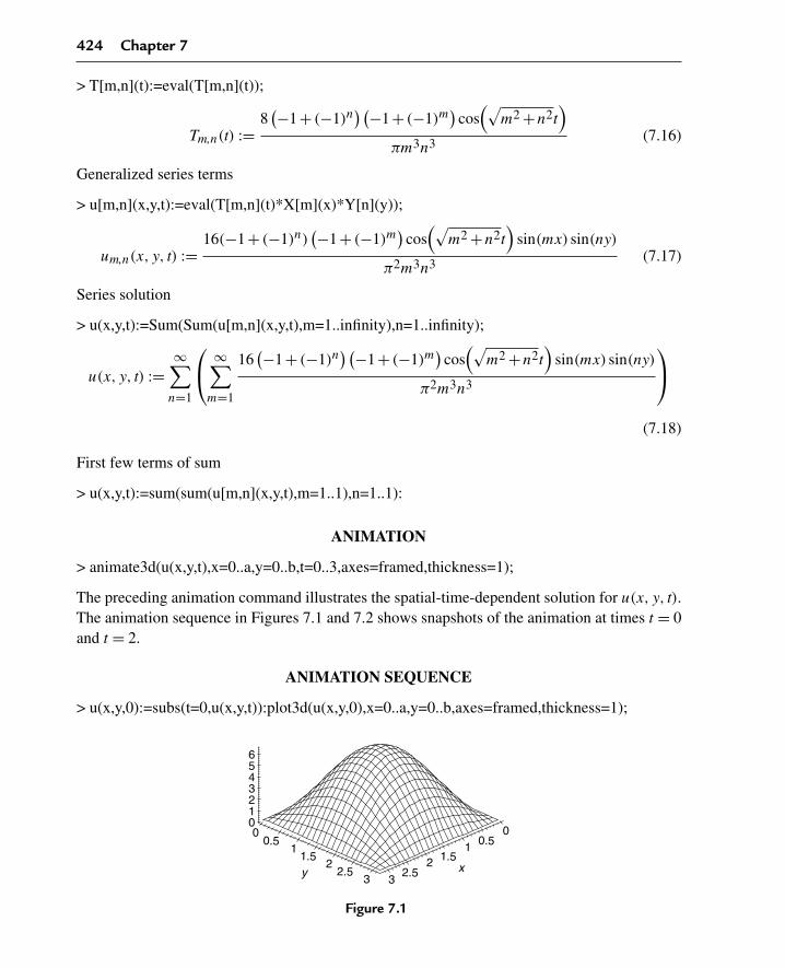
424 Chapter 7
> T[m,n](t):=eval(T[m,n](t));
Tm,n(t) :=8(−1+ (−1)n
) (−1+ (−1)m)
cos(√
m2 +n2t)
πm3n3(7.16)
Generalized series terms
> u[m,n](x,y,t):=eval(T[m,n](t)*X[m](x)*Y[n](y));
um,n(x, y, t) :=16(−1+ (−1)n)
(−1+ (−1)m)
cos(√
m2 +n2t)
sin(mx) sin(ny)
π2m3n3(7.17)
Series solution
> u(x,y,t):=Sum(Sum(u[m,n](x,y,t),m=1..infinity),n=1..infinity);
u(x, y, t) :=∞∑
n=1
⎛⎝ ∞∑
m=1
16(−1+ (−1)n
) (−1+ (−1)m)
cos(√
m2 +n2t)
sin(mx) sin(ny)
π2m3n3
⎞⎠
(7.18)
First few terms of sum
> u(x,y,t):=sum(sum(u[m,n](x,y,t),m=1..1),n=1..1):
ANIMATION
> animate3d(u(x,y,t),x=0..a,y=0..b,t=0..3,axes=framed,thickness=1);
The preceding animation command illustrates the spatial-time-dependent solution for u(x, y, t).The animation sequence in Figures 7.1 and 7.2 shows snapshots of the animation at times t = 0and t = 2.
ANIMATION SEQUENCE
> u(x,y,0):=subs(t=0,u(x,y,t)):plot3d(u(x,y,0),x=0..a,y=0..b,axes=framed,thickness=1);
6543210
y x
0.51
1.52
2.53
2.51.5
0.5
21
3
0 0
Figure 7.1

The Wave Equation in Two Spatial Dimensions 425
> u(x,y,2):=subs(t=2,u(x,y,t)):plot3d(u(x,y,2),x=0..a,y=0..b,axes=framed,thickness=1);
0212223242526
0
12
3 32
1
x
0.50.51.5
y2.5 2.5
1.5
0
Figure 7.2
EXAMPLE 7.6.2: We seek the wave amplitude u(x, y, t) for the transverse wave propagationon a thin rectangular membrane over the finite two-dimensional domain D = {(x, y) |0 < x < π,
0 < y < π}. The membrane is in a medium with zero damping, and the wave speed is c = 1/2.The boundaries x = 0 and x = π are unsecured and the boundaries y = 0 and y = π are heldfixed. The initial displacement distribution f(x, y) and the initial speed distribution g(x, y) aregiven as follows.
SOLUTION: The two-dimensional homogeneous wave equation is
∂2
∂t2u(x, y, t) = c2
(∂2
∂x2u(x, y, t)+ ∂2
∂y2u(x, y, t)
)−γ
(∂
∂tu(x, y, t)
)
The boundary conditions are type 2 at x = 0, type 2 at x = π, type 1 at y = 0, and type 1 aty = π:
ux(0, y, t) = 0 and ux(π, y, t) = 0
and
u(x,0, t) = 0 and u(x,π, t) = 0
The initial conditions are
u(x, y,0) = xy(π−y) and ut(x, y,0) = 0
The ordinary differential equations from the method of separation of variables are
d2
dt2T(t)+γ
(d
dtT(t)
)+ c2λT(t) = 0
d2
dx2X(x)+αX(x) = 0
d2
dy2Y(y)+βY(y) = 0

426 Chapter 7
The coupling equation reads
λ = α+β
The boundary conditions on the spatial equations are
Xx(0) = 0 and Xx(π) = 0
and
Y(0) = 0 and Y(π) = 0
Assignment of system parameters
> restart:with(plots):a:=Pi:b:=Pi:c:=1/2:unprotect(gamma):gamma:=0:
Allowed eigenvalues and orthonormal eigenfunctions are obtained from Examples 2.5.1and 2.5.3.
> alpha[m]:=(m*Pi/a)ˆ2;beta[n]:=(n*Pi/b)ˆ2;lambda[m,n]:=alpha[m]+beta[n];lambda[0,n]:=beta[n];
αm :=m2
βn :=n2
λm,n :=m2 +n2
λ0,n :=n2 (7.19)
for m = 0,1,2,3, . . . , and n = 1,2,3, . . . .
Orthonormal eigenfunctions
For m = 0,
> X[0](x):=1/sqrt(a);
X0(x) := 1√π
(7.20)
For m = 1,2,3, . . . ,
> X[m](x):=sqrt(2/a)*cos(m*Pi/a*x);X[r](x):=subs(m=r,X[m](x)):
Xm(x) :=√
2 cos(mx)√π
(7.21)
For n = 1,2,3, . . . ,

The Wave Equation in Two Spatial Dimensions 427
> Y[n](y):=sqrt(2/b)*sin(n*Pi/b*y);Y[s](y):=subs(n=s,Y[n](y)):
Yn(y) :=√
2 sin(ny)√π
(7.22)
Statements of orthonormality with their respective weight functions
> w(x):=1:Int(X[m](x)*X[r](x)*w(x),x=0..a)=delta(m,r);
π∫0
2 cos(mx) cos(rx)
πdx = δ(m, r) (7.23)
> w(y):=1:Int(Y[n](y)*Y[s](y)*w(y),y=0..b)=delta(n,s);
π∫0
2 sin(ny) sin(sy)
πdy = δ(n, s) (7.24)
Time-dependent solution
> T[m,n](t):=exp(−gamma/2*t)*(A(m,n)*cos(omega[m,n]*t)+B(m,n)*sin(omega[m,n]*t));
Tm,n(t) := A(m,n) cos(ωm,nt
)+B(m,n) sin(ωm,nt
)(7.25)
> T[0,n](t):=exp(−gamma/2*t)*(A(0,n)*cos(omega[0,n]*t)+B(0,n)*sin(omega[0,n]*t));
T0,n(t) := A(0, n) cos(ω0,nt
)+B(0, n) sin(ω0,nt
)(7.26)
Generalized series terms
> u[m,n](x,y,t):=T[m,n](t)*X[m](x)*Y[n](y);
um,n(x, y, t) := 2(A(m,n) cos
(ωm,nt
)+B(m,n) sin(ωm,nt
))cos(mx) sin(ny)
π(7.27)
> u[0,n](x,y,t):=T[0,n](t)*X[0](x)*Y[n](y);
u0,n(x, y, t) :=(A(0, n) cos
(ω0,nt
)+B(0, n) sin(ω0,nt
))√2 sin(ny)
π(7.28)
Eigenfunction expansion

428 Chapter 7
> u(x,y,t):=Sum(u[0,n](x,y,t),n=1..infinity)+Sum(Sum(u[m,n](x,y,t),m=1..infinity),n=1..infinity);
u(x, y, t) : =∞∑
n=1
(A(0, n) cos
(ω0,nt
)+B(0, n) sin(ω0,nt
))√2 sin(ny)
π
+∞∑
n=1
( ∞∑m=1
2(A(m,n) cos
(ωm,nt
)+B(m,n) sin(ωm,nt
))cos(mx) sin(ny)
π
)
(7.29)
> omega[m,n]:=sqrt(4*lambda[m,n]*cˆ2−gammaˆ2);
ωm,n :=√
m2 +n2 (7.30)
> omega[0,n]:=subs(m=0,omega[m,n]);
ω0,n :=√
n2 (7.31)
We consider the special case where the initial condition functions u(x, y,0) = f(x, y) andut(x, y,0) = g(x, y) are given as
> f(x,y):=x*y*(Pi−y);
f(x, y) := xy(π−y) (7.32)
> g(x,y):=0;
g(x, y) := 0 (7.33)
From Section 7.5, the double Fourier coefficients A(m,n) and B(m,n) are determined from theintegrals
For m = 1,2,3, . . . , and n = 1,2,3, . . . ,
> A(m,n):=eval(Int(Int(f(x,y)*X[m](x)*w(x)*Y[n](y)*w(y),x=0..a),y=0..b));A(m,n):=expand(value(%)):
A(m,n) :=π∫
0
π∫0
2xy(π−y) cos(mx) sin(ny)
πdxdy (7.34)
> A(m,n):=factor(subs({sin(m*Pi)=0,cos(m*Pi)=(−1)ˆm,sin(n*Pi)=0,cos(n*Pi)=(−1)ˆn},A(m,n)));
A(m,n) := −4(−1+ (−1)n
) (−1+ (−1)m)
πm2n3(7.35)

The Wave Equation in Two Spatial Dimensions 429
> B(m,n):=eval(Int(Int((f(x,y)*gamma/2+g(x,y))/(omega[m,n])*X[m](x)*Y[n](y),x=0..a),y=0..b));B(m,n):=expand(value(%)):
B(m,n) :=π∫
0
π∫0
0 dxdy (7.36)
> B(m,n):=simplify(subs({sin(m*Pi)=0,cos(m*Pi)=(−1)ˆm,sin(n*Pi)=0,cos(n*Pi)=(−1)ˆn},B(m,n)));
B(m,n) := 0 (7.37)
For m = 0 and n = 1, 2,3, . . . ,
> A(0,n):=eval(Int(Int(f(x,y)*X[0](x)*w(x)*Y[n](y)*w(y),x=0..a),y=0..b));A(0,n):=expand(value(%)):
A(0, n) :=π∫
0
π∫0
xy(π−y)√
2 sin(ny)
πdxdy (7.38)
> A(0,n):=simplify(subs({sin(m*Pi)=0,cos(m*Pi)=(−1)ˆm,sin(n*Pi)=0,cos(n*Pi)=(−1)ˆn},A(0,n)));
A(0, n) := −π√
2(−1+ (−1)n
)n3
(7.39)
> B(0,n):=eval(Int(Int((f(x,y)*gamma/2+g(x,y))/(omega[0,n])*X[0](x)*Y[n](y),x=0..a),y=0..b));B(0,n):=expand(value(%)):
B(0, n) :=π∫
0
π∫0
0 dxdy (7.40)
> B(0,n):=simplify(subs({sin(m*Pi)=0,cos(m*Pi)=(−1)ˆm,sin(n*Pi)=0,cos(n*Pi)=(−1)ˆn},B(0,n)));
B(0, n) := 0 (7.41)
> T[m,n](t):=eval(T[m,n](t));
Tm,n(t) := −4(−1+ (−1)n
) (−1+ (−1)m)
cos(√
m2 +n2 t)
πm2n3(7.42)

430 Chapter 7
> T[0,n](t):=eval(T[0,n](t));
T0,n(t) := −π√
2(−1+ (−1)n
)cos
(√n2 t
)n3
(7.43)
Generalized series terms
> u[m,n](x,y,t):=eval(T[m,n](t)*X[m](x)*Y[n](y));
um,n(x, y, t) := −8(−1+ (−1)n
) (−1+ (−1)m)
cos(√
m2 +n2 t)
cos(mx) sin(ny)
π2m2n3(7.44)
> u[0,n](x,y,t):=eval(T[0,n](t)*X[0](x)*Y[n](y));
u0,n(x, y, t) := −2(−1+ (−1)n
)cos
(√n2t
)sin(ny)
n3(7.45)
Series solution
> u(x,y,t):=Sum(u[0,n](x,y,t),n=1..infinity)+Sum(Sum(u[m,n](x,y,t),m=1..infinity),n=1..infinity);
u(x, y, t) :=∞∑
n=1
⎛⎝−
2(−1+ (−1)n
)cos
(√n2t
)sin(ny)
n3
⎞⎠+
∞∑n=1
⎛⎝ ∞∑
m=1
⎛⎝−
8(−1+ (−1)n
) (−1+ (−1)m)
cos(√
m2 +n2t)
cos(mx) sin(ny)
π2m2n3
⎞⎠⎞⎠
(7.46)
First few terms of sum
> u(x,y,t):=sum(u[0,n](x,y,t),n=1..1)+sum(sum(u[m,n](x,y,t),m=1..1),n=1..1):
ANIMATION
> animate3d(u(x,y,t),x=0..a,y=0..b,t=0..3,axes=framed,thickness=1);
The preceding animation command illustrates the spatial-time-dependent solution for u(x, y, t).The animation sequence in Figures 7.3 and 7.4 shows snapshots of the animation at times t = 0and t = 2.
ANIMATION SEQUENCE
> u(x,y,0):=subs(t=0,u(x,y,t)):plot3d(u(x,y,0),x=0..a,y=0..b,axes=framed,thickness=1);

The Wave Equation in Two Spatial Dimensions 431
7654321
00
1
2
3 32
1
x
0.50.5
1.5y 2.5 2.5
1.5
0
Figure 7.3
> u(x,y,2):=subs(t=2,u(x,y,t)):plot3d(u(x,y,2),x=0..a,y=0..b,axes=framed,thickness=1);
10
21222324
0
1
2
3 3
2
1
x
0.50.5
1.5y
2.5 2.5
1.5
0
Figure 7.4
EXAMPLE 7.6.3: We seek the wave amplitude u(x, y, t) for the transverse wave propagationon a thin rectangular membrane over the finite two-dimensional domain D = {(x, y) |0 < x < 1,
0 < y < 1}. The membrane is in a medium with no damping and the wave speed is c = 1/2.The boundaries x = 0, x = 1, and y = 0 are held fixed, and the boundary y = 1 is constrained tomove on an elastic hinge. The initial displacement function f(x, y) and the initial speedfunction g(x, y) are given as follows.
SOLUTION: The two-dimensional homogeneous wave equation is
∂2
∂t2u(x, y, t) = c2
(∂2
∂x2u(x, y, t)+ ∂2
∂y2u(x, y, t)
)−γ
(∂
∂tu(x, y, t)
)
The boundary conditions are type 1 at x = 0, type 1 at x = 1, type 1 at y = 0, and type 3 at y = 1:
u(0, y, t) = 0 and u(1, y, t) = 0
and
u(x,0, t) = 0 and u(x,1, t)+uy(x,1, t) = 0
432 Chapter 7
The initial conditions are
u(x, y,0) = xy(1−x)
8and ut(x, y,0) = 0
The ordinary differential equations from the method of separation of variables are
d2
dt2T(t)+γ
(d
dtT(t)
)+ c2λT(t) = 0
d2
dx2X(x)+αX(x) = 0
d2
dy2Y(y)+βY(y) = 0
The coupling equation reads
λ = α+β
The boundary conditions on the spatial equations are
X(0) = 0 and X(1) = 0
and
Y(0) = 0 and Y(1)+Yy(1) = 0
Assignment of system parameters
> restart:with(plots):a:=1:b:=1:c:=1/2:unprotect(gamma):gamma:=0:
Allowed eigenvalues and corresponding orthonormal eigenfunctions are obtained fromExamples 2.5.1 and 2.5.4.
> alpha[m]:=(m*Pi/a)ˆ2;lambda[m,n]:=alpha[m]+beta[n];
αm :=m2π2
λm,n :=m2π2 +βn (7.47)
for m = 1,2,3, . . . , and n = 1,2,3, . . . , where βn are the roots of the eigenvalue equation
> tan(sqrt(beta[n])*b)=−sqrt(beta[n]);
tan(√
βn
)= −√
βn (7.48)
Orthonormal eigenfunctions
> X[m](x):=sqrt(2/a)*sin(m*Pi/a*x);X[r](x):=subs(m=r,X[m](x)):
Xm(x) := √2 sin(mπx) (7.49)

The Wave Equation in Two Spatial Dimensions 433
> Y[n](y):=sqrt(2)*(1/sqrt((cos(sqrt(beta[n])*b)ˆ2+b)))*sin(sqrt(beta[n])*y);Y[s](y):=subs(n=s,Y[n](y)):
Yn(y) :=√
2 sin(√
βny)
√cos
(√βn
)2 +1(7.50)
Statements of orthonormality with their respective weight functions
> w(x):=1:Int(X[m](x)*X[r](x)*w(x),x=0..a)=delta(m,r);
1∫0
2 sin(mπx) sin(rπx)dx = δ(m, r) (7.51)
> w(y):=1:Int(Y[n](y)*Y[s](y)*w(y),y=0..b)=delta(n,s);
1∫0
2 sin(√
βny)
sin(√
βsy)
√cos
(√βn
)2 +1√
cos(√
βs
)2 +1dy = δ(n, s) (7.52)
Time-dependent solution
> T[m,n](t):=exp(−gamma/2*t)*(A(m,n)*cos(omega[m,n]*t)+B(m,n)*sin(omega[m,n]*t));
Tm,n(t) := A(m,n) cos(ωm,nt
)+B(m,n) sin(ωm,nt
)(7.53)
Generalized series terms
> u[m,n](x,y,t):=T[m,n](t)*X[m](x)*Y[n](y);
um,n(x, y, t) := 2(A(m,n) cos
(ωm,nt
)+B(m,n) sin(ωm,nt
))sin(mπx) sin
(√βny
)√
cos(√
βn
)2 +1(7.54)
Eigenfunction expansion
> u(x,y,t):=Sum(Sum(u[m,n](x,y,t),m=1..infinity),n=1..infinity);
u(x, y, t) :=∞∑
n=1
⎛⎜⎝ ∞∑
m=1
2(A(m,n) cos
(ωm,nt
)+B(m,n) sin(ωm,nt
))sin(mπx) sin
(√βn y
)√
cos(√
βn
)2 +1
⎞⎟⎠
(7.55)
> omega[m,n]:=sqrt(4*lambda[m,n]*cˆ2−gammaˆ2);
ωm,n :=√
m2π2 +βn (7.56)

434 Chapter 7
We consider the special case where the initial condition functions u(x, y,0) = f(x, y) andut(x, y,0) = g(x, y) are given as
> f(x,y):=x*y*(1−x)/8;
f(x, y) := 1
8xy(1−x) (7.57)
> g(x,y):=0;
g(x, y) := 0 (7.58)
From Section 7.5, the double Fourier coefficients A(m,n) and B(m,n) are determined from theintegrals:
> A(m,n):=eval(Int(Int(f(x,y)*X[m](x)*w(x)*Y[n](y)*w(y),x=0..a),y=0..b));A(m,n):=expand(value(%)):
A(m,n) :=1∫
0
1∫0
1
4
xy(1−x) sin(mπx) sin(√
βny)
√cos
(√βn
)2 +1dxdy (7.59)
> A(m,n):=simplify(subs({sin(sqrt(beta[n])*b)=−sqrt(beta[n])*cos(sqrt(beta[n])*b),sin(m*Pi)=0,cos(m*Pi)=(−1)ˆm},A(m,n)));
A(m,n) := cos(√
βn
) (−1+ (−1)m)
m3π3√βn
√cos
(√βn
)2 +1(7.60)
> B(m,n):=eval(Int(Int((f(x,y)*gamma/2+g(x,y))/(omega[m,n])*X[m](x)*Y[n](y),x=0..a),y=0..b));B(m,n):=expand(value(%)):
B(m,n) :=1∫
0
1∫0
0 dxdy (7.61)
> B(m,n):=simplify(subs({sin(sqrt(beta[n])*b)=−sqrt(beta[n])*cos(sqrt(beta[n])*b),sin(m*Pi)=0,cos(m*Pi)=(−1)ˆm},B(m,n)));
B(m,n) := 0 (7.62)
> T[m,n](t):=eval(T[m,n](t));
Tm,n(t) :=cos
(√βn
) (−1+ (−1)m)
cos(√
m2π2 +βn t)
m3π3√βn
√cos
(√βn
)2 +1(7.63)
Generalized series terms

The Wave Equation in Two Spatial Dimensions 435
> u[m,n](x,y,t):=eval(T[m,n](t)*X[m](x)*Y[n](y));
um,n(x, y, t) :=2 cos
(√βn
) (−1+ (−1)m)
cos(√
m2π2 +βn t)
sin(mπx) sin(√
βny)
m3π3√βn
(cos
(√βn
)2 +1) (7.64)
Series solution
> u(x,y,t):=Sum(Sum(u[m,n](x,y,t),m=1..infinity),n=1..infinity);
u(x, y, t) :=∞∑
n=1
⎛⎝ ∞∑
m=1
2 cos(√
βn
) (−1+ (−1)m)
cos(√
m2π2 +βnt)
sin(mπx) sin(√
βn y)
m3π3√βn
(cos
(√βn
)2 +1)
⎞⎠
(7.65)
Evaluation of the eigenvalues βn from the roots of the eigenvalue equation yields
> tan(sqrt(beta[n])*b)+sqrt(beta[n])=0;
tan(√
βn
)+√
βn = 0 (7.66)
> plot({tan(v),−v},v=0..20,y=−20..0,thickness=10);
v5 10 15 20
y
220
215
210
25
0
Figure 7.5
If we set v = √βb, then the eigenvalues βn are found from the intersection points of the curves
shown in Figure 7.5. Some of these eigenvalues using the Maple fsolve command areevaluated here:
> beta[1]:=(1/bˆ2)*(fsolve((tan(v)+v),v=1..3))ˆ2;
β1 := 4.115858365 (7.67)
> beta[2]:=(1/bˆ2)*(fsolve((tan(v)+v),v=3..6))ˆ2;
β2 := 24.13934203 (7.68)

436 Chapter 7
> beta[3]:=(1/bˆ2)*(fsolve((tan(v)+v),v=6..9))ˆ2;
β3 := 63.65910654 (7.69)
First few terms of sum
> u(x,y,t):=eval(sum(sum(u[m,n](x,y,t),m=1..3),n=1..3)):
ANIMATION
> animate3d(u(x,y,t),x=0..a,y=0..b,t=0..3,axes=framed,thickness=1);
The preceding animation command illustrates the spatial-time-dependent solution for u(x, y, t).The animation sequence in Figures 7.6 and 7.7 shows snapshots of the animation at the twotimes t = 0 and t = 4.
ANIMATION SEQUENCE
> u(x,y,0):=subs(t=0,u(x,y,t)):plot3d(u(x,y,0),x=0..a,y=0..b,axes=framed,thickness=1);
0.0250.02
0.0150.01
0.00500
0.20.4
0.60.8
1 10.8
0.60.4
xy
0.20
Figure 7.6
> u(x,y,4):=subs(t=4,u(x,y,t)):plot3d(u(x,y,4),x=0..a,y=0..b,axes=framed,thickness=1);
20.00520.01
20.0220.015
0
00.2
0.4y 0.6
0.81 1
0.80.6
0.4x
0.20
Figure 7.7

The Wave Equation in Two Spatial Dimensions 437
7.7 Wave Equation in the Cylindrical Coordinate System
If we replace the Laplacian operator from Section 7.2 in rectangular coordinates in twodimensions to its equivalent in cylindrical coordinates, then the nonhomogeneous partialdifferential equation for wave phenomena in the cylindrical coordinate system in twodimensions is given as
∂2
∂t2u(r, θ, t) = c2
⎛⎝ ∂
∂r u (r, θ, t)+ r(
∂2
∂r2 u(r, θ, t))
r+
∂2
∂θ2 u(r, θ, t)
r2
⎞⎠−γ
(∂
∂tu(r, θ, t)
)+h(r, θ, t)
where r is the coordinate radius of the system and θ is the polar angle. The γ term takes intoaccount any viscous damping in the medium, and h(r, θ, t) takes into account any externalapplied forces acting on the system. There is no z dependence here because we will onlyexamine wave phenomena along very thin membranes or plates that have no extension alongthe z-axis.
As for the rectangular coordinate system, we can write the preceding equation in terms of thelinear operator for the wave equation in cylindrical coordinates as
L(u) = h(r, θ, t)
where the wave operator in cylindrical coordinates reads
L(u) = ∂2
∂t2u(r, θ, t)− c2
⎛⎝ ∂
∂r u(r, θ, t)+ r(
∂2
∂r2 u(r, θ, t))
r+
∂2
∂θ2 u(r, θ, t)
r2
⎞⎠+γ
(∂
∂tu(r, θ, t)
)
Generally, one seeks a solution to this equation over the finite two-dimensional domainD = {(r, θ) |0 < r < a,0 < θ < b} subject to the following homogeneous boundary conditions:
|u(0, θ, t)| < ∞κ1u(a, θ, t)+κ2ur(a, θ, t) = 0
κ3u(r,0, t)+κ4uθ(r,0, t) = 0
κ5u(r, b, t)+κ6uθ(r, b, t) = 0
along with the two initial conditions
u(r, θ,0) = f(r, θ) and ut(r, θ,0) = g(r, θ)
We now attempt to solve the homogeneous version [no external applied forces, h(r, θ, t) = 0] ofthis partial differential equation using the method of separation of variables. We set
u(r, θ, t) = R(r)�(θ)T(t)

438 Chapter 7
Substituting this into the preceding homogeneous partial differential equation, we get
R(r)�(θ)
(d2
dt2T(t)
)+γR(r)�(θ)
(d
dtT(t)
)
= c2
⎛⎝
(ddr
R(r))
�(θ)T(t)+ r(
d2
dr2 R(r))
�(θ)T(t)
r+
R(r)(
d2
dθ2 �(θ))
T(t)
r2
⎞⎠
Dividing both sides by the product solution yields
d2
dt2T(t)+γ
(ddt
T(t))
c2T(t)=
�(θ)r(
ddr
R(r))
+�(θ)r2(
d2
dr2 R(r))
+R(r)(
d2
dθ2 �(θ))
R(r)�(θ)r2
Because the left-hand side is an exclusive function of t and the right-hand side an exclusivefunction of r and θ, and r, θ, and t are independent, the only way we can ensure equality of thepreceding for all values of r, θ, and t is to set each side equal to a constant. Doing so, we arriveat the following three ordinary differential equations in terms of the separation constants (forconvenience here, we square the constants to ensure positivity):
d2
dt2T(t)+γ
(d
dtT(t)
)+ c2λ2T(t) = 0
d2
dθ2�(θ)+μ2�(θ) = 0
r2
(d2
dr2R(r)
)+ r
(d
drR(r)
)+
(λ2r2 −μ2
)R(r) = 0
The preceding differential equation in t is an ordinary second-order linear equation for whichwe already have the solution from Chapter 1. The second differential equation in the variable θ
is recognized as being an Euler-type differential equation for which we generated solutions inSection 1.4. The third differential equation is a Bessel-type differential equation whosesolutions are Bessel functions of the first kind of order μ as shown in Section 1.11.
We easily recognize each of the two spatial differential equations in θ and r, with theircorresponding boundary conditions, as being Sturm-Liouville-type differential equations.
We first consider the differential equation with respect to the variable θ subject to thehomogeneous boundary conditions over the finite interval I = {θ |0 < θ < b}. TheSturm-Liouville problem for the θ-dependent portion of the wave equation consists of theordinary differential equation
d2
dθ2�(θ)+μ2�(θ) = 0

The Wave Equation in Two Spatial Dimensions 439
along with its respective corresponding regular homogeneous boundary conditions
κ3�(0)+κ4�θ(0) = 0
and
κ5�(b)+κ6�θ(b) = 0
We recognize this problem in the variable θ to be a regular Sturm-Liouville eigenvalueproblem whereby the allowed values of μ are called the system “eigenvalues” and thecorresponding solutions are called the “eigenfunctions.” Note that the ordinary differentialequation given is of the Euler type, and the weight function is w(θ) = 1. The indexedeigenvalues and corresponding eigenfunctions are given, respectively, as
μm,�m(θ)
for m = 0,1,2,3, . . . .
These eigenfunctions can be normalized and the corresponding statement of orthonormalitywith respect to the weight function w(θ) = 1 reads
b∫0
�m(θ)�q(θ)dθ = δ(m,q)
We now consider the r-dependent differential equation over the finite intervalI = {r |0 < r < a}. The Sturm-Liouville problem for the r-dependent portion of the waveequation consists of the ordinary differential equation
r2
(d2
dr2R(r)
)+ r
(d
drR(r)
)+
(λ2r2 −μ2
)R(r) = 0
along with its respective corresponding nonregular homogeneous boundary conditions
|R(0)| < ∞and
κ1R(a)+κ2Rr(a) = 0
As discussed in Chapters 1 and 2 on the Bessel differential equation, we recognize this problemin the spatial variable r as a singular Sturm-Liouville eigenvalue problem. This comes about,since the differential equation fails to be “normal” at the origin. Nevertheless, the singularproblem can be solved, and the allowed values of λ are called the system “eigenvalues” and thecorresponding solutions are called the “eigenfunctions.” We note that the allowed values of λ
are also dependent on the values of μ. The ordinary differential equation given is of the Bessel

440 Chapter 7
type, and, from Section 2.6, the weight function is w(r) = r. The indexed eigenvalues andcorresponding eigenfunctions are given, respectively, as
λm,n,Rm,n(r)
for m = 0,1,2,3, . . . , and n = 0,1,2,3, . . . .
Again, these eigenfunctions can be normalized and the corresponding statement oforthonormality with respect to the weight function w(r) = r reads
a∫0
Rm,n(r)Rm,p(r)r dr = δ(n,p)
What was stated in Section 2.2 about regular Sturm-Liouville eigenvalue problems in onedimension can be extended to two dimensions here; that is, the product of the aboveeigenfunctions in r and θ form a “complete” set with respect to any piecewise smooth functionf(r, θ) over the finite two-dimensional domain D = {(r, θ) |0 < r < a,0 < θ < b}.Finally, we focus on the time-dependent equation, which reads
d2
dt2T(t)+γ
(d
dtT(t)
)+ c2λ2T(t) = 0
For the indexed values of λm,n given, the solution to this second-order differential equationfrom Section 1.4 is
Tm,n(t) = e− γ t2
⎛⎜⎝A(m,n) cos
⎛⎜⎝
√4λ2
m,nc2 −γ2 t
2
⎞⎟⎠+B(m,n) sin
⎛⎜⎝
√4λ2
m,nc2 −γ2 t
2
⎞⎟⎠
⎞⎟⎠
where the coefficients A(m,n) and B(m,n) are unknown arbitrary constants.
Throughout most of our example problems, we make the assumption of small damping in thesystem—that is,
γ2 < 4λ2m,nc2
This assumption yields time-dependent solutions that are oscillatory. The argument of the sineand cosine expressions denotes the angular frequency of the (m,n) term in the system. Thedamped angular frequency of oscillation of the (m,n)th term or mode is given formally as
ωm,n =√
4λ2m,nc2 −γ2
2
Thus, by the method of separation of variables, we arrive at an infinite number of indexedsolutions for the homogeneous wave partial differential equation, over a finite domain. Thesesolutions are(
um,n
)(r, θ, t) = Rm,n(r)�m(θ)e− γ t
2(A(m,n) cos
(ωm,nt
)+B(m,n) sin(ωm,nt
))for m = 0,1,2,3, . . . , and n = 0,1,2,3, . . . .

The Wave Equation in Two Spatial Dimensions 441
Using arguments similar to those used for the regular Sturm-Liouville problem given earlier,we can write our general solution to the partial differential equation as the superposition of theproducts of the solutions to each of the preceding ordinary differential equations.
Thus, the generalized solution to the homogeneous wave partial differential equation can bewritten as the double infinite sum
u(r, θ, t) =∞∑
n=0
( ∞∑m=0
Rm,n(r)�m(θ)e−γ t2
(A(m,n) cos
(ωm,nt
)+B(m,n) sin(ωm,nt
)))(7.70)
The unknown Fourier coefficients A(m,n) and B(m,n) are to be evaluated from the initialconditions on the problem. We now demonstrate an illustrative example problem.
DEMONSTRATION: We seek the wave amplitude u(r, θ, t) for transverse waves on a thincircular membrane in a viscous medium over the two-dimensional domainD = {(r, θ) |0 < r < 1,0 < θ < π/2}. The damping coefficient is zero and the wave speed isc = 1/2. The plate is fixed at θ = 0, at θ = π/2, and at the outer periphery (r = 1). The initialdisplacement function f(r, θ) and the initial speed function g(r, θ) are given as follows.
SOLUTION: The two-dimensional homogeneous wave equation in cylindrical coordinatesreads
4
(∂2
∂t2u(r, θ, t)
)=
∂∂r u(r, θ, t)+ r
(∂2
∂r2 u(r, θ, t))
r+
∂2
∂θ2 u(r, θ, t)
r2
The boundary conditions are type 1 at r = 1, type 1 at θ = 0, type 1 at θ = π/2, and we requirea finite solution at the origin:
u(1, θ, t) = 0 and |u(0, θ, t)| < ∞and
u(r,0, t) = 0 and u(r,
π
2, t
)= 0
The initial conditions are
u(r, θ,0) = f(r, θ) and ut(r, θ,0) = g(r, θ)
The ordinary differential equations from the method of separation of variables are
d2
dt2T(t)+ λ2T(t)
4= 0
d2
dθ2�(θ)+μ2�(θ) = 0
r2
(d2
dr2R(r)
)+ r
(d
drR(r)
)+
(λ2r2 −μ2
)R(r) = 0

442 Chapter 7
The boundary conditions on the spatial variables are
�(0) = 0 and �(π
2
)= 0
and
|R(0)| < ∞ and R(1) = 0
We consider the θ-dependent equation first. Here, we have a Sturm-Liouville differentialequation of the Euler type with weight function w(θ) = 1. The allowed eigenvalues andcorresponding orthonormal eigenfunctions, from Example 2.5.1, are
μm = 2m
and
�m(θ) = 2 sin(2mθ)√π
for m = 1,2,3, . . . .
We next consider the r-dependent equation. This is a Sturm-Liouville differential equation ofthe Bessel type with weight function w(r) = r. From Example 2.6.2, the eigenvalues λm,n arethe roots of the eigenvalue equation
J(2m,λm,n
) = 0
for m = 1,2,3, . . . , and n = 1,2,3, . . . . Here, J(2m,λm,n
)is the Bessel function of the first
kind of order 2m. The corresponding orthonormalized r-dependent eigenfunctions are
Rm,n(r) = J(2m,λm,nr
)√∫ 1
0J(2m,λm,nr
)2r dr
The statements of orthonormality, with their respective weight functions, are
1∫0
J(2m,λm,nr
)J(2m,λm,pr
)r√∫ 1
0J(2m,λm,nr
)2r dr
√∫ 1
0J(2m,λm,pr
)2r dr
dr = δ(n,p)
andπ2∫
0
4 sin(2mθ) sin(2qθ)
πdθ = δ(m,q)
for m,q = 1,2,3, . . . , and n,p = 1,2,3, . . . .
The Wave Equation in Two Spatial Dimensions 443
Finally, we focus on the time-dependent differential equation, which reads
d2
dt2T(t)+ λ2
m,nT(t)
4= 0
The solution to this second-order differential equation from Section 1.4 is
Tm,n = A(m,n) cos(ωm,nt
)+B(m,n) sin(ωm,nt
)where ωm,n is the undamped angular frequency
ωm,n = λm,n
2
Forming the superposition of the product of the solutions to each of the preceding threeordinary differential equations, the general eigenfunction expansion solution to the partialdifferential equation reads
u(r, θ, t) =∞∑
n=1
⎛⎜⎜⎜⎜⎝
∞∑m=1
2(A(m,n) cos
(ωm,nt
)+B(m,n) sin(ωm,nt
))J(m,λm,nr
)sin(2mθ)
√π
√∫ 1
0J(2m,λm,nr
)2r dr
⎞⎟⎟⎟⎟⎠
The Fourier coefficients A(m,n) and B(m,n) are to be determined from the initial conditionfunctions u(r, θ,0) = f(r, θ) and ut(r, θ,0) = g(r, θ).
7.8 Initial Conditions for the Wave Equation in CylindricalCoordinates
We now consider the initial conditions on the problem. At time t = 0, let the initialdisplacement distribution be given as
u(r, θ,0) = f(r, θ)
and the initial speed distribution be
ut(r, θ,0) = g(r, θ)
Substituting the first condition into the following general solution
u(r, θ, t) =∞∑
n=0
( ∞∑m=0
Rm,n(r)�m(θ)e−γ t2
(A(m,n) cos
(ωm,nt
)+B(m,n) sin(ωm,nt
)))

444 Chapter 7
at time t = 0 yields
f(r, θ) =∞∑
n=0
( ∞∑m=0
Rm,n(r)�m(θ)A(m,n)
)
Substituting the second condition into the time derivative of the solution at time t = 0 yields
g(r, θ) =∞∑
n=0
( ∞∑m=0
(B(m,n)ωm,n − A(m,n)γ
2
)Rm,n(r)�m(θ)
)
Because the eigenfunctions of the Sturm-Liouville problem form a complete set with respect topiecewise smooth functions over the finite two-dimensional domain, the preceding sums arethe generalized double Fourier series expansions of the functions f(r, θ) and g(r, θ) in terms ofthe allowed eigenfunctions. We can evaluate the unknown Fourier coefficients A(m,n) andB(m,n) by taking advantage of the given familiar orthonormality statements.
Similar to what was done in Section 2.4 for the generalized Fourier series expansion in onevariable, we evaluate the double Fourier coefficients A(m,n) and B(m,n) as follows. We takethe double inner products of both sides of the preceding equations, with respect to the r- andθ-dependent eigenfunctions, and we assume the validity of the interchange between thesummation and integration operators. For the first equation we get
b∫0
a∫0
f(r, θ)Rq,p(r)�q(θ)r dr dθ =
∞∑n=0
⎛⎝ ∞∑
m=0
A(m,n)
⎛⎝ a∫
0
Rq,p(r)Rm,n(r)r dr
⎞⎠
⎛⎝ b∫
0
�m(θ)�q(θ)dθ
⎞⎠
⎞⎠
Taking advantage of the given orthonormality statements, the first condition yields
b∫0
a∫0
f(r, θ)Rq,p(r)�q(θ)r dr dθ =∞∑
n=0
( ∞∑m=0
A(m,n)δ(n,p)δ(m,q)
)
Due to the mathematical nature of the Kronecker delta function, only the n = p, m = q termsurvives the sum and the double Fourier coefficient A(m,n) reads
A(m,n) =b∫
0
a∫0
f(r, θ)Rm,n(r)�m(θ)r dr dθ

The Wave Equation in Two Spatial Dimensions 445
For the second condition, we get
b∫0
a∫0
g(r, θ)Rq,p(r)�q(θ)r dr dθ =
∞∑n=0
⎛⎝ ∞∑
m=0
(B(m,n)ωm,n − A(m,n)γ
2
)⎛⎝ a∫
0
Rq,p(r)Rm,n(r)r dr
⎞⎠
⎛⎝ b∫
0
�m(θ)�q(θ)dθ
⎞⎠
⎞⎠
Again, taking advantage of the given orthonormality statements, the second condition yields
b∫0
a∫0
g(r, θ)Rq,p(r)�q(θ)r dr dθ =∞∑
n=0
( ∞∑m=0
(B(m,n)ωm,n − A(m,n)γ
2
)δ(n,p)δ(m,q)
)
(7.71)
Again, due to the mathematical nature of the Kronecker delta function, only the n = p,m = q
term survives the sum, and, combining the previous value for A(m,n), the double Fouriercoefficient B(m,n) reads
B(m,n) =b∫
0
a∫0
(f(r,θ)γ
2 +g(r, θ))
rRm,n(r)�m(θ)
ωm,ndr dθ
We now demonstrate the evaluation of the Fourier coefficients for the example problem fromSection 7.7.
DEMONSTRATION: We consider the special case where the initial temperature distributionfunction u(r, θ,0) = f(r, θ) is given as
f(r, θ) =(r2 − r4
)sin(2θ)
and the initial speed distribution function is ut(r, θ,0) = g(r, θ) where
g(r, θ) = 0
SOLUTION: From the preceding, the Fourier coefficients A(m,n) and B(m,n) are evaluatedby taking the double inner product of the initial condition functions with respect to thecorresponding orthonormal eigenfunctions. For the coefficient A(m,n), we have the integral
A(m,n) =1∫
0
π2∫
0
(r2 − r4
)sin(2θ)Rm,n(r)r�m(θ)dθ dr

446 Chapter 7
where, from the example, the orthonormalized eigenfunctions are
�m(θ) = 2 sin(2mθ)√π
and
Rm,n(r) = J(2m,λm,nr
)√∫ 1
0J(2m,λm,nr
)2r dr
for m = 1,2,3,. . . , and n = 1,2,3, . . . . Insertion of these eigenfunctions into the precedingintegral yields
A(m,n) =1∫
0
π2∫
0
(r2 − r4) sin(2θ)Rm,n(r)r ·2 sin(2mθ)√π
dθ dr
Integrating first with respect to θ, and noting that f(r, θ) depends on the term sin(2mθ) for thecase m = 1, then from the statement of orthonormality for θ, we see that only the m = 1 termsurvives here. Thus, we are left with the integral
A(1, n) =1∫
0
π2∫
0
(r2 − r4) sin(2θ)2R1,n(r)r ·2√π
dθ dr
where, for m = 1,
R1,n = J(2, λ1,nr)√∫ 1
0J(2, λ1,nr)2r dr
Evaluation of R1,n yields
R1,n = J(2, λ1,nr)√
2
J(1, λ1,n)
Inserting this into A(1, n) and integrating twice yields
A(1, n) = −6√
2π
λ31,n
for n = 1, 2,3, . . . . Since there is no damping in the system and the initial speed distributiong(r, θ) = 0, the integral for B(m,n) is zero. Thus, the final solution to the problem reads
u(r, θ, t) =∞∑
n=1
⎛⎝−
24 cos(
λ1,nt
2
)J(2, λ1,nr) sin(2θ)
λ31,n
J(1, λ1,n)
⎞⎠

The Wave Equation in Two Spatial Dimensions 447
The preceding solution is completed on evaluation of the eigenvalues λ1,n from the eigenvalueequation
J(2, λ1,n) = 0
The details for the development of the solution and the graphics are given later in one of theMaple worksheets.
7.9 Example Wave Equation Problems in CylindricalCoordinates
We now consider several examples of partial differential equations for wave phenomena undervarious homogeneous boundary conditions over finite two-dimensional domains in thecylindrical coordinate system. We note that the r-dependent ordinary differential equations inthe cylindrical coordinate system are of the Bessel type and the θ-dependent equations are ofthe Euler type.
EXAMPLE 7.9.1: We seek the wave amplitude u(r, θ, t) for transverse waves on a thin circularmembrane in a viscous medium over the two-dimensional domain D = {(r, θ)|0 < r < 1,
0 < θ < π/2}. The damping coefficient γ is zero and the wave speed is c = 1/2. The plate isfixed at θ = 0, θ = π/2, and at the outer periphery (r = 1). The initial displacement functionf(r, θ) and the initial speed distribution g(r, θ)) are given as follows.
SOLUTION: The two-dimensional homogeneous wave equation in cylindrical coordinatesreads
∂2
∂t2u(r, θ, t)+γ
(∂
∂tu(r, θ, t)
)= c2
⎛⎝ ∂
∂r u(r, θ, t)+ r(
∂2
∂r2 u(r, θ, t))
r+
∂2
∂θ2 u(r, θ, t)
r2
⎞⎠
The boundary conditions are type 1 at r = 1, type 1 at θ = 0, type 1 at θ = π/2, and we requirea finite solution at the origin:
u(1, θ, t) = 0 and |u(0, θ, t)| < ∞
and
u(r,0, t) = 0 and u(r,
π
2, t
)= 0
The initial conditions are
u(r, θ,0) =(r2 − r4
)sin(2θ) and ut(r, θ,0) = 0

448 Chapter 7
The ordinary differential equations from the method of separation of variables are
d2
dt2T(t)+γ
(d
dtT(t)
)+ c2λ2T(t) = 0
d2
dθ2�(θ)+μ2�(θ) = 0
r2
(d2
dr2R(r)
)+ r
(d
drR(r)
)+
(λ2r2 −μ2
)R(r) = 0
The boundary conditions on the spatial variables are
�(0) = 0 and �(π
2
)= 0
and|R(0)| < ∞ and R(1) = 0
Assignment of system parameters
> restart:with(plots):a:=1:b:=Pi/2:c:=1/2:unprotect(gamma):gamma:=0:
Allowed eigenvalues and corresponding orthonormal eigenfunctions are obtained fromExamples 2.5.1 and 2.6.2.
> mu[m]:=m*Pi/b;
μm := 2m (7.72)
Eigenvalues λm,n are the roots of the eigenvalue equation
> BesselJ(mu[m],lambda[m,n]*a)=0;
BesselJ(2m,λm,n) = 0 (7.73)
for m = 1,2,3, . . . , and n = 1,2,3, . . . .
Orthonormal eigenfunctions
> Theta[m](theta):=sqrt(2/b)*sin(m*Pi/b*theta);Theta[q](theta):=subs(m=q,Theta[m](theta)):
�m(θ) := 2 sin(2mθ)√π
(7.74)
> R[m,n](r):=BesselJ(mu[m],lambda[m,n]*r)/sqrt(Int(BesselJ(mu[m],lambda[m,n]*r)ˆ2*r,r=0..a));R[m,p](r):=subs(n=p,R[m,n](r)):
Rm,n(r) := BesselJ(2m,λm,nr
)√∫ 1
0BesselJ
(2m,λm,nr
)2r dr
(7.75)

The Wave Equation in Two Spatial Dimensions 449
Statements of orthonormality with their respective weight functions
> w(r):=r:Int(R[m,n](r)*R[m,p](r)*w(r),r=0..a)=delta(n,p);
1∫0
BesselJ(2m,λm,nr)BesselJ(2m,λm,pr)r√∫ 1
0BesselJ
(2m,λm,nr
)2r dr
√∫ 1
0BesselJ
(2m,λm,pr
)2r dr
dr = δ(n,p) (7.76)
> w(theta):=1:Int(Theta[m](theta)*Theta[q](theta)*w(theta),theta=0..b)=delta(m,q);
12 π∫
0
4 sin(2mθ) sin(2qθ)
πdθ = δ(m,q) (7.77)
Time-dependent solution
> T[m,n](t):=exp(−gamma/2*t)*(A(m,n)*cos(omega[m,n]*t)+B(m,n)*sin(omega[m,n]*t));
Tm,n(t) := A(m,n) cos(ωm,nt
)+B(m,n) sin(ωm,nt
)(7.78)
Generalized series terms
> u[m,n](r,theta,t):=T[m,n](t)*R[m,n](r)*Theta[m](theta);
um,n(r, θ, t) := 2(A(m,n) cos
(ωm,nt
)+B(m,n) sin(ωm,nt
))BesselJ
(2m,λm,nr
)sin(2mθ)√∫ 1
0BesselJ
(2m,λm,nr
)2r dr
√π
(7.79)
Eigenfunction expansion
> u(r,theta,t):=Sum(Sum(u[m,n](r,theta,t),m=1..infinity),n=1..infinity);
u(r, θ, t) :=∞∑
n=1
⎛⎜⎜⎜⎜⎝
∞∑m=1
2(A(m,n) cos
(ωm,nt
)+B(m,n) sin(ωm,nt
))BesselJ
(2 m,λm,nr
)sin(2mθ)√∫ 1
0BesselJ
(2m,λm,nr
)2r dr
√π
⎞⎟⎟⎟⎟⎠
(7.80)
> omega[m,n]:=sqrt(4*lambda[m,n]ˆ2*cˆ2−gammaˆ2)/2;
ωm,n := 1
2
√λ2
m,n (7.81)
We consider the special case where the initial condition functions u(r, θ,0) = f(r, θ) andut(r, θ,0) = g(r, θ) are given as

450 Chapter 7
> f(r,theta):=(rˆ2−rˆ4)*sin(2*theta);
f(r, θ) :=(r2 − r4
)sin(2θ) (7.82)
> g(r,theta):=0;
g(r, θ) := 0 (7.83)
Because f(r, θ) depends on the term sin(2mθ) for the case where m = 1, then from the givenorthonormality statement for θ, only the m = 1 term survives here and we set
> Theta[1](theta):=subs(m=1,eval(Theta[m](theta)));
�1(θ) := 2 sin(2θ)√π
(7.84)
> omega[1,n]:=subs(m=1,omega[m,n]);
ω1,n := 1
2
√λ2
1,n(7.85)
Eigenvalues λ1,n are the roots of the eigenvalue equation
> subs({m=1,r=a},BesselJ(mu[m],lambda[1,n]*r))=0;
BesselJ(2, λ1,n
) = 0 (7.86)
For m = 1, we have the Bessel identity
> subs(m=1,BesselJ(0,lambda[m,n]*a)=2*BesselJ(1,lambda[m,n]*a)/(lambda[m,n]*a)−BesselJ(2,lambda[m,n]*a));
BesselJ(0, λ1,n
) = 2BesselJ(1, λ1,n
)λ1,n
−BesselJ(2, λ1,n
)(7.87)
Evaluation of the eigenfunctions and the Fourier coefficients with the preceding substitutionsyields
> R[1,n](r):=eval(subs(m=1,BesselJ(mu[m],lambda[m,n]*r)/sqrt(expand(int(subs(m=1,BesselJ(mu[m],lambda[m,n]*r))ˆ2*r,r=0..a)))));
R1,n(r) := 2BesselJ(2, λ1,nr
)√
2BesselJ(0, λ1,n
)2 +2BesselJ(1, λ1,n
)2 − 8BesselJ(1,λ1,n)2
λ21,n
(7.88)
The Wave Equation in Two Spatial Dimensions 451
Substitution of the eigenvalue equation and the preceding Bessel identity simplifies this
> R[1,n](r):=radsimp(subs(BesselJ(0,lambda[1,n]*a)=2*BesselJ(1,lambda[1,n]*a)/(lambda[1,n]*a),R[1,n](r)));
R1,n(r) := BesselJ(2, λ1,nr
)√2
BesselJ(1, λ1,n
) (7.89)
From Section 7.8, the double Fourier coefficients A(m,n) and B(m,n) are determined from theintegrals
> A(1,n):=Int(Int(f(r,theta)*R[1,n](r)*Theta[1](theta)*w(r),r=0..a),theta=0..b);
A(1, n) :=12 π∫
0
1∫0
2(r2 − r4
)sin(2θ)2 BesselJ
(2, λ1,nr
)√2r
BesselJ(1, λ1,n
)√π
dr dθ (7.90)
> A(1,n):=radsimp(subs(BesselJ(0,lambda[1,n]*a)=2*BesselJ(1,lambda[1,n]*a)/(lambda[1,n]*a),value(%)));
A(1, n) := −6√
π√
2
λ31,n
(7.91)
> B(1,n):=Int(Int((f(r,theta)*gamma/2+g(r,theta))/omega[1,n]*R[1,n](r)*Theta[1](theta)*w(r),r=0..a),theta=0..b);
B(1, n) :=12 π∫
0
1∫0
0 dr dθ (7.92)
> B(1,n):=radsimp(subs(BesselJ(0,lambda[1,n]*a)=2*BesselJ(1,lambda[1,n]*a)/(lambda[1,n]*a),value(%)));
B(1, n) := 0 (7.93)
> T[1,n](t):=eval(subs(m=1,T[m,n](t)));
T1,n(t) := −6
√π
√2 cos
(12
√λ2
1,nt)
λ31,n
(7.94)
Generalized series terms
> u[1,n](r,theta,t):=eval(T[1,n](t)*R[1,n](r)*Theta[1](theta));
u1,n(r, θ, t) := −24 cos
(12
√λ2
1,nt)
BesselJ(2, λ1,nr
)sin(2θ)
λ31,n
BesselJ(1, λ1,n
) (7.95)

452 Chapter 7
Series solution
> u(r,theta,t):=Sum(u[1,n](r,theta,t),n=1..infinity);
u(r, θ, t) :=∞∑
n=1
⎛⎜⎝−
24 cos(
12
√λ2
1,nt)
BesselJ(2, λ1,nr
)sin(2θ)
λ31,n
BesselJ(1, λ1,n
)⎞⎟⎠ (7.96)
Evaluation of the eigenvalues from the roots of the eigenvalue equation yields
> subs(m=1,BesselJ(mu[m],lambda[m,n]*a)=0);
BesselJ(2, λ1,n
) = 0 (7.97)
> plot(BesselJ(2,v),v=0..20,thickness=10);
0.4
0.3
0.2
0.1
05 10
v15 20
20.1
20.2
20.3
Figure 7.8
If we set v = λa, then the eigenvalues λ1,n are found from the intersection points of the curvesof J(2, v) with the v-axis shown in Figure 7.8. Some of these eigenvalues are calculated hereusing the Maple fsolve command
> lambda[1,1]:=(1/a)*fsolve(BesselJ(2,v)=0,v=1..6);
λ1,1 := 5.135622302 (7.98)
> lambda[1,2]:=(1/a)*fsolve(BesselJ(2,v)=0,v=6..10);
λ1,2 := 8.417244140 (7.99)
> lambda[1,3]:=(1/a)*fsolve(BesselJ(2,v)=0,v=10..14);
λ1,3 := 13.32369194 (7.100)
First few terms in sum
> u(r,theta,t):=sum(u[1,n](r,theta,t),n=1..1):
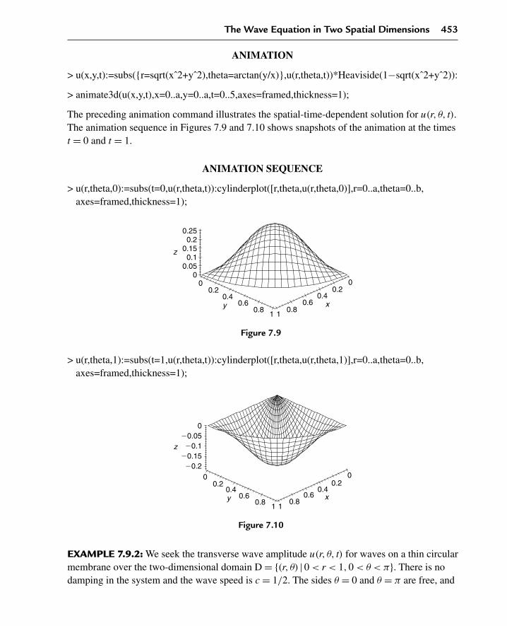
The Wave Equation in Two Spatial Dimensions 453
ANIMATION
> u(x,y,t):=subs({r=sqrt(xˆ2+yˆ2),theta=arctan(y/x)},u(r,theta,t))*Heaviside(1−sqrt(xˆ2+yˆ2)):
> animate3d(u(x,y,t),x=0..a,y=0..a,t=0..5,axes=framed,thickness=1);
The preceding animation command illustrates the spatial-time-dependent solution for u(r, θ, t).The animation sequence in Figures 7.9 and 7.10 shows snapshots of the animation at the timest = 0 and t = 1.
ANIMATION SEQUENCE
> u(r,theta,0):=subs(t=0,u(r,theta,t)):cylinderplot([r,theta,u(r,theta,0)],r=0..a,theta=0..b,axes=framed,thickness=1);
0.150.1
00.05
0.250.2
00.2
0.4y
z
0.60.8
1 10.8
0.60.4
x
0.20
Figure 7.9
> u(r,theta,1):=subs(t=1,u(r,theta,t)):cylinderplot([r,theta,u(r,theta,1)],r=0..a,theta=0..b,axes=framed,thickness=1);
20.1520.1
020.05
20.20
0.20.4y
z
0.60.8 1 1
0.80.6
0.4x
0.20
Figure 7.10
EXAMPLE 7.9.2: We seek the transverse wave amplitude u(r, θ, t) for waves on a thin circularmembrane over the two-dimensional domain D = {(r, θ) |0 < r < 1,0 < θ < π}. There is nodamping in the system and the wave speed is c = 1/2. The sides θ = 0 and θ = π are free, and

454 Chapter 7
the edge r = 1 is held fixed. The initial displacement function f(r, θ) and the initial speedfunction g(r, θ) are given as follows.
SOLUTION: The two-dimensional homogeneous wave equation in cylindrical coordinatesreads
∂2
∂t2u(r, θ, t)+γ
(∂
∂tu(r, θ, t)
)= c2
⎛⎝ ∂
∂r u(r, θ, t)+ r(
∂2
∂r2 u(r, θ, t))
r+
∂2
∂θ2 u(r, θ, t)
r2
⎞⎠
The boundary conditions are type 1 at r = 1, type 2 at θ = 0, type 2 at θ = π, and we require afinite solution at the origin:
u(1, θ, t) = 0 and |u(0, θ, t)| < ∞and
uθ(r,0, t) = 0 and uθ(r,π, t) = 0
The initial conditions are
u(r, θ,0) = r2 cos(2θ) and ut(r, θ,0) = 0
The ordinary differential equations from the method of separation of variables are
d2
dt2T(t)+γ
(d
dtT(t)
)+ c2λ2T(t) = 0
d2
dθ2�(θ)+μ2�(θ) = 0
r2
(d2
dr2R(r)
)+ r
(d
drR(r)
)+
(λ2r2 −μ2
)R(r) = 0
The boundary conditions on the spatial variables are
�θ(0) = 0 and �θ(π) = 0
and
|R(0)| < ∞ and R(1) = 0
Assignment of system parameters
> restart:with(plots):a:=1:b:=Pi:c:=1/2:unprotect(gamma):gamma:=0:
Allowed eigenvalues and corresponding orthonormal eigenfunctions are obtained fromExamples 2.5.3 and 2.6.2. For m = 1,2,3, . . . , n = 1,2,3,. . . ,
> mu[m]:=m*Pi/b;
μm := m (7.101)

The Wave Equation in Two Spatial Dimensions 455
Eigenvalues λm,n are the roots of the eigenvalue equation
> BesselJ(mu[m],lambda[m,n]*a)=0;
BesselJ(m,λm,n
) = 0 (7.102)
Orthonormal eigenfunctions
> R[m,n](r):=BesselJ(mu[m],lambda[m,n]*r)/sqrt(Int(BesselJ(mu[m],lambda[m,n]*r)ˆ2*r,r=0..a));R[m,p](r):=subs(n=p,R[m,n](r)):
Rm,n(r) := BesselJ(m,λm,nr
)√∫ 1
0BesselJ
(m,λm,nr
)2r dr
(7.103)
> Theta[m](theta):=sqrt(2/b)*cos(m*Pi/b*theta);Theta[q](theta):=subs(m=q,Theta[m](theta)):
�m(θ) :=√
2 cos(mθ)√π
(7.104)
For m = 0, n = 1,2,3, . . . , λ0,n are the roots of the equation
> BesselJ(0,lambda[0,n]*a)=0;
BesselJ(0, λ0,n
) = 0 (7.105)
Orthonormal eigenfunctions
> R[0,n](r):=BesselJ(0,lambda[0,n]*r)/sqrt(Int(BesselJ(0,lambda[0,n]*r)ˆ2*r,r=0..a));R[0,p](r):=subs(n=p,R[0,n](r)):
R0,n(r) := BesselJ(0, λ0,nr
)√∫ 1
0BesselJ
(0, λ0,nr
)2r dr
(7.106)
> Theta[0](theta):=sqrt(1/b);
�0(θ) := 1√π
(7.107)
Statements of orthonormality with their respective weight functions
> w(r):=r:Int(R[m,n](r)*R[m,p](r)*w(r),r=0..a)=delta(n,p);
1∫0
BesselJ(m,λm,nr
)BesselJ
(m,λm,pr
)r√∫ 1
0BesselJ
(m,λm,nr
)2r dr
√∫ 1
0BesselJ
(m,λm,pr
)2r dr
dr = δ(n,p) (7.108)

456 Chapter 7
> w(theta):=1:Int(Theta[m](theta)*Theta[q](theta)*w(theta),theta=0..b)=delta(m,q);
π∫0
2 cos(mθ) cos(qθ)
πdθ = δ(m,q) (7.109)
Time-dependent solution
> T[m,n](t):=exp(−gamma/2*t)*(A(m,n)*cos(omega[m,n]*t)+B(m,n)*sin(omega[m,n]*t));u[m,n](r,theta,t):=eval(T[m,n](t)*R[m,n](r)*Theta[m](theta)):
Tm,n(t) := A(m,n) cos(ωm,nt
)+B(m,n) sin(ωm,nt
)(7.110)
> T[0,n](t):=exp(−gamma/2*t)*(A(0,n)*cos(omega[0,n]*t)+B(0,n)*sin(omega[0,n]*t));u[0,n](r,theta,t):=T[0,n](t)*R[0,n](r)*Theta[0](theta):
T0,n(t) := A(0, n) cos(ω0,nt
)+B(0, n) sin(ω0,nt
)(7.111)
Eigenfunction expansion
> u(r,theta,t):=Sum(u[0,n](r,theta,t),n=1..infinity)+Sum(Sum(u[m,n](r,theta,t),m=1..infinity),n=1..infinity);
u(r, θ, t) : =∞∑
n=1
(A(0, n) cos
(ω0,nt
)+B(0, n) sin(ω0,nt
))BesselJ
(0, λ0,nr
)√∫ 1
0BesselJ
(0, λ0,nr
)2r dr
√π
+∞∑
n=1
⎛⎜⎜⎜⎜⎝
∞∑m=1
(A(m,n) cos
(ωm,nt
)+B(m,n) sin(ωm,nt
))BesselJ
(m,λm,nr
)√2 cos(mθ)√∫ 1
0BesselJ
(m,λm,nr
)2r dr
√π
⎞⎟⎟⎟⎟⎠
(7.112)
> omega[m,n]:=sqrt(4*lambda[m,n]ˆ2*cˆ2−gammaˆ2)/2;
ωm,n := 1
2
√λ2
m,n (7.113)
We consider the special case where the initial condition functions u(r, θ,0) = f(r, θ) andut(r, θ,0) = g(r, θ) are given as
> f(r,theta):=rˆ2*cos(2*theta);
f(r, θ) := r2 cos(2θ) (7.114)

The Wave Equation in Two Spatial Dimensions 457
> g(r,theta):=0;
g(r, θ) := 0 (7.115)
Since f(r, θ) depends on the term cos(mθ) for the case where m = 2, then from the givenorthonormality statement for θ, only the m = 2 term survives here and we set
> Theta[2](theta):=subs(m=2,eval(Theta[m](theta)));
�2(θ) :=√
2 cos(2θ)√π
(7.116)
> omega[2,n]:=subs(m=2,omega[m,n]);
ω2,n := 1
2
√λ2
2,n(7.117)
Eigenvalues λ2,n are the roots of the eigenvalue equation
> subs(m=2,BesselJ(mu[m],lambda[m,n]*a)=0);
BesselJ(2, λ2,n
) = 0 (7.118)
To simplify our answer, we take advantage of the Bessel identity
> BesselJ(0,lambda[2,n]*a)=2*BesselJ(1,lambda[2,n]*a)/(lambda[2,n]*a)−BesselJ(2,lambda[2,n]*a);
BesselJ(0, λ2,n
) = 2BesselJ(1, λ2,n
)λ2,n
−BesselJ(2, λ2,n
)(7.119)
Evaluation of the eigenfunctions and the Fourier coefficients with the preceding substitutionsyields
> R[2,n](r):=eval(subs(m=2,BesselJ(mu[m],lambda[m,n]*r)/sqrt(expand(int(subs(m=2,BesselJ(mu[m],lambda[m,n]*r))ˆ2*r,r=0..a)))));
R2,n(r) := 2BesselJ(2, λ2,nr
)√
2BesselJ(0, λ2,n
)2 +2BesselJ(1, λ2,n
)2 − 8BesselJ(1,λ2,n)2
λ22,n
(7.120)
Substitution of the eigenvalue equation and the preceding Bessel identity simplifies this
> R[2,n](r):=radsimp(subs(BesselJ(0,lambda[2,n]*a)=2*BesselJ(1,lambda[2,n]*a)/(lambda[2,n]*a),R[2,n](r)));
R2,n(r) := BesselJ(2, λ2,nr
)√2
BesselJ(1, λ2,n
) (7.121)
458 Chapter 7
From Section 7.8, the double Fourier coefficients A(m,n) and B(m,n) are determined from theintegrals
> A(2,n):=Int(Int(f(r,theta)*R[2,n](r)*Theta[2](theta)*w(r),r=0..a),theta=0..b);
A(2, n) :=π∫
0
1∫0
2r3 cos(2θ)2 BesselJ(2, λ2,nr
)BesselJ
(1, λ2,n
)√π
dr dθ (7.122)
> A(2,n):=subs(BesselJ(0,lambda[2,n]*a)=2*BesselJ(1,lambda[2,n]*a)/(lambda[2,n]*a),value(%));
A(2, n) := −√
π
λ2,n(7.123)
> B(2,n):=Int(Int((f(r,theta)*gamma/2+g(r,theta))/(omega[2,n])*R[2,n](r)*Theta[2](theta)*w(r),r=0..a),theta=0..b);
B(2, n) :=π∫
0
1∫0
0 dr dθ (7.124)
> B(2,n):=value(%);
B(2, n) := 0 (7.125)
> T[2,n](t):=eval(subs(m=2,T[m,n](t)));
T2,n(t) := −√
π cos(
12
√λ2
2,nt)
λ2,n(7.126)
Generalized series terms
> u[2,n](r,theta,t):=eval(T[2,n](t)*R[2,n](r)*Theta[2](theta));
u2,n(r, θ, t) := −2 cos
(12
√λ2
2,nt)
BesselJ(2, λ2,nr
)cos(2θ)
λ2,nBesselJ(1, λ2,n
) (7.127)
Series solution
> u(r,theta,t):=Sum(u[2,n](r,theta,t),n=1..infinity);
u(r, θ, t) :=∞∑
n=1
⎛⎜⎝−
2 cos(
12
√λ2
2,nt)
BesselJ(2, λ2,nr
)cos(2θ)
λ2,nBesselJ(1, λ2,n
)⎞⎟⎠ (7.128)
Evaluation of the eigenvalues λ2,n from the roots of the eigenvalue equation yields

The Wave Equation in Two Spatial Dimensions 459
> subs({r=a,m=2},BesselJ(mu[m],lambda[m,n]*r))=0;
BesselJ(2, λ2,n
) = 0 (7.129)
> plot(BesselJ(2,v),v=0..20,thickness=10);
0.4
0.3
0.2
20.1
20.2
20.3
0
0.1
5 10v
15 20
Figure 7.11
If we set v = λa, then the eigenvalues λ2,n are the roots of the equation J(2, v) shown inFigure 7.11. A few of these eigenvalues are evaluated here using the Maple fsolve command
> lambda[2,1]:=(1/a)*fsolve(BesselJ(2,v)=0,v=1..6);
λ2,1 := 5.135622302 (7.130)
> lambda[2,2]:=(1/a)*fsolve(BesselJ(2,v)=0,v=6..10);
λ2,2 := 8.417244140 (7.131)
> lambda[2,3]:=(1/a)*fsolve(BesselJ(2,v)=0,v=10..14);
λ2,3 := 11.61984117 (7.132)
First few terms in sum
> u(r,theta,t):=sum(u[2,n](r,theta,t),n=1..1):
ANIMATION
> u(x,y,t):=subs({r=sqrt(xˆ2+yˆ2),theta=arccos(x/sqrt(xˆ2+yˆ2))},u(r,theta,t))*Heaviside(1-sqrt(xˆ2+yˆ2)):
> animate3d(u(x,y,t),x=-a..a,y=0..a,t=0..5,axes=framed,thickness=1);
The preceding animation command illustrates the spatial-time-dependent solution for u(r, θ, t).The animation sequence in Figures 7.12 and 7.13 shows snapshots of the animation at the timest = 0 and t = 4.

460 Chapter 7
ANIMATION SEQUENCE
> u(r,theta,0):=subs(t=0,u(r,theta,t)):cylinderplot([r,theta,u(r,theta,0)],r=0..a,theta=0..b,axes=framed,thickness=1);
0.40.2
20.220.4
00.2
0.40.6
0.811
0.50
20.521
0z
y x
Figure 7.12
> u(r,theta,4):=subs(t=4,u(r,theta,t)):cylinderplot([r,theta,u(r,theta,4)],r=0..a,theta=0..b,axes=framed,thickness=1);
20.320.220.1
00.10.20.3
0
0.4
0.5
20.521
00.60.8
1 1x
0.2
y
z
Figure 7.13
EXAMPLE 7.9.3: We seek the wave amplitude u(r, θ, t) for transverse waves on a thincircularly symmetric membrane in a viscous medium over the two-dimensional domainD = {(r, θ) |0 < r < 1, 0 < θ < 2π}. The damping coefficient γ is very small and the wavespeed is c = 1. The membrane is clamped at its circular edge. The initial displacement functionf(r) and the initial speed function g(r) are given as follows. Because the membrane iscircularly symmetric and the initial distributions are θ-independent, then the solution is alsoθ-independent.
SOLUTION: The two-dimensional homogeneous wave equation in cylindrical coordinates fora θ-independent system reads
∂2
∂t2u(r, t)+γ
(∂
∂tu(r, t)
)=
c2(
∂∂r u(r, t)+ r
(∂2
∂r2 u(r, t)))
r

The Wave Equation in Two Spatial Dimensions 461
The boundary conditions are type 1 at r = 1, and we require a finite solution at the origin:
u(1, t) = 0 and |u(0, t)| < ∞The initial conditions are
u(r,0) = 1− r2 and ut(r,0) = 0
The ordinary differential equations from the method of separation of variables are
d2
dt2T (t)+γ
(d
dtT(t)
)+ c2λ2T(t) = 0
r2
(d2
dr2R(r)
)+ r
(d
drR(r)
)+λ2r2R(r) = 0
The boundary conditions on the r equation are
|R(0)| < ∞ and R(1) = 0
Assignment of system parameters
> restart:with(plots):a:=1:c:=1:unprotect(gamma):gamma:=1/2:
The r-dependent equation is a Bessel differential equation of the first kind of order m = 0. Theallowed eigenvalues and corresponding orthonormal eigenfunctions are obtained fromExample 2.6.2. The eigenvalues λ0,n are the roots of the eigenvalue equation
> subs(r=a,BesselJ(0,lambda[0,n]*r))=0;
BesselJ(0, λ0,n
) = 0 (7.133)
for n = 1,2,3, . . . .
Orthonormal eigenfunctions
> R[0,n](r):=BesselJ(0,lambda[0,n]*r)/sqrt(Int(BesselJ(0,lambda[0,n]*r)ˆ2*r,r=0..a));R[0,p](r):=subs(n=p,R[0,n](r)):
R0,n(r) := BesselJ(0, λ0,nr
)√∫ 1
0BesselJ
(0, λ0,nr
)2r dr
(7.134)
Statement of orthonormality with weight function w(r) = r
> w(r):=r:Int(R[0,n](r)*R[0,p](r)*w(r),r=0..a)=delta(n,p);
1∫0
BesselJ(0, λ0,nr
)BesselJ
(0, λ0,pr
)r√∫ 1
0BesselJ
(0, λ0,nr
)2r dr
√∫ 1
0BesselJ
(0, λ0,pr
)2r dr
dr = δ(n,p) (7.135)
462 Chapter 7
Time-dependent solution
> T[0,n](t):=exp(−gamma/2*t)*(A(0,n)*cos(omega[0,n]*t)+B(0,n)*sin(omega[0,n]*t));
T0,n(t) := e− 14 t
(A(0, n) cos
(ω0,nt
)+B(0, n) sin(ω0,nt
))(7.136)
Generalized series terms
> u[0,n](r,t):=T[0,n](t)*R[0,n](r);
u0,n(r, t) := e− 14 t
(A(0, n) cos
(ω0,nt
)+B(0, n) sin(ω0,nt
))BesselJ
(0, λ0,nr
)√∫ 1
0 BesselJ(0, λ0,nr
)2r dr
(7.137)
Eigenfunction expansion
> u(r,t):=Sum(u[0,n](r,t),n=1..infinity);
u(r, t) :=∞∑
n=1
e− 14 t
(A(0, n) cos
(ω0,nt
)+B(0, n) sin(ω0,nt
))BesselJ
(0, λ0,nr
)√∫ 1
0 BesselJ(0, λ0,nr
)2r dr
(7.138)
> omega[0,n]:=sqrt(4*lambda[0,n]ˆ2*cˆ2−gammaˆ2)/2;
ω0,n := 1
4
√16λ2
0,n−1 (7.139)
We consider the special case where the initial condition functions u(r, θ,0) = f(r, θ) andut(r, θ,0) = g(r, θ) are given as
> f(r):=1−rˆ2;
f(r) := 1− r2 (7.140)
> g(r):=0;
g(r) := 0 (7.141)
Eigenvalues λ0,n are the roots of the eigenvalue equation
> subs(r=a,BesselJ(0,lambda[0,n]*r))=0;
BesselJ(0, λ0,n
) = 0 (7.142)
Evaluation of the eigenfunctions yields
> R[0,n](r):=eval(BesselJ(0,lambda[0,n]*r)/sqrt(int(BesselJ(0,lambda[0,n]*r)ˆ2*r,r=0..a)));
R0,n(r) := BesselJ(0, λ0,nr
)√2√√
πλ0,nBesselJ(0,λ0,n)2+√
πλ0,nBesselJ(1,λ0,n)2
√πλ0,n
(7.143)
The Wave Equation in Two Spatial Dimensions 463
Substitution of the eigenvalue equation in the preceding simplifies this
> R[0,n](r):=radsimp(subs(BesselJ(0,lambda[0,n]*a)=0,R[0,n](r)));
R0,n(r) := BesselJ(0, λ0,nr
)√2
BesselJ(1, λ0,n
) (7.144)
From Section 7.8, the double Fourier coefficients A(m,n) and B(m,n) are determined from theintegrals:
> A(0,n):=Int(f(r)*R[0,n](r)*w(r),r=0..a);
A(0, n) :=1∫
0
(1− r2
)BesselJ
(0, λ0,nr
)√2r
BesselJ(1, λ0,n
) dr (7.145)
> A(0,n):=simplify(subs(BesselJ(0,lambda[0,n]*a)=0,value(%)));
A(0, n) := 4√
2
λ30,n
(7.146)
> B(0,n):=Int((f(r)*gamma/2+g(r))/omega[0,n]*R[0,n](r)*w(r),r=0..a);
B(0, n) :=1∫
0
4(
14 − 1
4r2)
BesselJ(0, λ0,nr
)√2 r√
16λ20,n
−1 BesselJ(1, λ0,n
) dr (7.147)
> B(0,n):=simplify(subs(BesselJ(0,lambda[0,n]*a)=0,value(%)));
B(0, n) := 4√
2
λ30,n
√16λ2
0,n−1
(7.148)
> T[0,n](t):=(eval(T[0,n](t)));
T0,n(t) := e− 14 t
⎛⎜⎝4
√2 cos
(14
√16λ2
0,n−1t
)λ3
0,n
+4√
2 sin(
14
√16λ2
0,n−1t
)λ3
0,n
√16λ2
0,n−1
⎞⎟⎠ (7.149)

464 Chapter 7
Generalized series terms
> u[0,n](r,t):=eval(T[0,n](t)*R[0,n](r));
u0,n(r, t) := 1
BesselJ(1, λ0, n)
⎛⎜⎝e− 1
4 t
⎛⎜⎝4
√2 cos
(14
√16λ2
0,n−1 t
)λ3
0,n
+4√
2 sin(
14
√16λ2
0,n−1 t
)λ3
0,n
√16λ2
0,n−1
⎞⎟⎠BesselJ(0, λ0,nr)
√2
⎞⎟⎠ (7.150)
Series solution
> u(r,t):=Sum(u[0,n](r,t),n=1..infinity);
u(r, t) :=∞∑
n=1
1
BesselJ(1, λ0,n)
⎛⎜⎝e− 1
4 t
⎛⎜⎝4
√2 cos
(14
√16λ2
0,n−1 t
)λ3
0,n
+4√
2 sin(
14
√16λ2
0,n−1 t
)λ3
0,n
√16λ2
0,n−1
⎞⎟⎠BesselJ(0, λ0,nr)
√2
⎞⎟⎠ (7.151)
Evaluation of eigenvalues λ0,n from the roots of the eigenvalue equation yields
> subs(r=a,BesselJ(0,lambda[0,n]*r)=0);
BesselJ(0, λ0,n) = 0 (7.152)
> plot(BesselJ(0,v),v=0..20,thickness=10);
If we set v = λa, then the eigenvalues λ0,n are the roots of the equation J(0, v) shown inFigure 7.14. Evaluation of some of these eigenvalues using the Maple fsolve command yields
1
0.8
0.6
20.2
20.4
0
0.2
0.4
10 15 20
v
5
Figure 7.14

The Wave Equation in Two Spatial Dimensions 465
> lambda[0,1]:=(1/a)*fsolve(BesselJ(0,v)=0,v=1..4);
λ0,1 := 2.404825558 (7.153)
> lambda[0,2]:=(1/a)*fsolve(BesselJ(0,v),v=4..7);
λ0,2 := 5.520078110 (7.154)
> lambda[0,3]:=(1/a)*fsolve(BesselJ(0,v)=0,v=7..11);
λ0,3 := 8.653727913 (7.155)
First few terms in sum
> u(r,t):=sum(u[0,n](r,t),n=1..3):
ANIMATION
> u(x,y,t):=subs(r=sqrt(xˆ2+yˆ2),u(r,t))*Heaviside(1−sqrt(xˆ2+yˆ2)):
> animate3d(u(x,y,t),x=−a..a,y=−a..a,t=0..3,axes=framed,thickness=1);
The preceding animation command illustrates the spatial-time-dependent solution for u(r, t).The animation sequence in Figures 7.15 and 7.16 shows snapshots of the animation at the timest = 0 and t = 2.
ANIMATION SEQUENCE
> u(r,0):=subs(t=0,u(r,t)):cylinderplot([r,theta,u(r,0)],r=0..a,theta=0..2*Pi,axes=framed,thickness=1);
0
0
0.20.4
0.51 1
0.50
0.60.8
1
20.521
20.521
z
y x
Figure 7.15
> u(r,2):=subs(t=2,u(r,t)):cylinderplot([r,theta,u(r,2)],r=0..a,theta=0..2*Pi,axes=framed,thickness=1);

466 Chapter 7
00.5
1 10.5
0
0
20.5
20.0220.015
20.0120.005
2120.5
21
z
y x
Figure 7.16
Chapter Summary
Nonhomogeneous wave equation in two dimensions in rectangular coordinates
∂2
∂t2u(x, y, t) = c2
(∂2
∂x2u(x, y, t)+ ∂2
∂y2u(x, y, t)
)−γ
(∂
∂tu(x, y, t)
)+h(x, y, t)
Linear wave operator in two dimensions in rectangular coordinates
L(u) = ∂2
∂t2u(x, y, t)+γ
(∂
∂tu(x, y, t)
)− c2
(∂2
∂x2u(x, y, t)+ ∂2
∂y2u(x, y, t)
)
The method of separation of variables solution
u(x, y, t) = X(x)Y(y)T(t)
Eigenfunction expansion solution for rectangular coordinates
u(r, y, t) =∞∑
n=0
( ∞∑m=0
Xm(x)Yn(y)e−γt2 (A(m,n) cos(ωm,nt)+B(m,n) sin(ωm,nt))
)
Fourier coefficients from initial conditions for rectangular coordinates
A(m,n) =b∫
0
a∫0
f(x, y)Xm(x)Yn(y)dxdy
and
B(m,n) =b∫
0
a∫0
(f(x,y)γ
2 +g(x, y))
Xm(x)Yn(y)
ωm,ndxdy
The Wave Equation in Two Spatial Dimensions 467
Nonhomogeneous wave equation in two dimensions in cylindrical coordinates
∂2
∂t2u(r, θ, t) = c2
⎛⎝ ∂
∂r u(r, θ, t)+ r(
∂2
∂r2 u(r, θ, t))
r+
∂2
∂θ2 u(r, θ, t)
r2
⎞⎠−γ
(∂
∂tu(r, θ, t)
)+h(r, θ, t)
Linear wave operator in two dimensions in cylindrical coordinates
L(u) = ∂2
∂t2u(r, θ, t)+γ
(∂
∂tu(r, θ, t)
)− c2
⎛⎝ ∂
∂r u(r, θ, t)+ r(
∂2
∂r2 u(r, θ, t))
r+
∂2
∂θ2 u(r, θ, t)
r2
⎞⎠
The method of separation of variables solution
u(r, θ, t) = R(r)�(θ)T(t)
Eigenfunction expansion solution in cylindrical coordinates
u(r, θ, t) =∞∑
n=0
( ∞∑m=0
Rm,n(r)�m(θ)e−γt2 (A(m,n) cos(ωm,nt)+B(m,n) sin(ωm,nt))
)
Initial condition Fourier coefficients for cylindrical coordinates
A(m,n) =b∫
0
a∫0
f(r, θ)Rm,n(r)�m(θ) r dr dθ
and
B(m,n) =b∫
0
a∫0
(f(r,θ)γ
2 +g(r, θ))
Rm,n(r)�m(θ)r
ωm,ndr dθ
We have examined homogeneous partial differential equations describing wave phenomena intwo spatial dimensions for both the rectangular and the cylindrical coordinate systems.
Exercises
We now consider problems for the wave equation with homogeneous boundary conditions intwo dimensions in both the rectangular and cylindrical coordinate systems. We use the methodof separation of variables and eigenfunction expansions to evaluate the solutions.
Two Dimensions, Rectangular Coordinates
We consider the transverse wave distribution in thin membranes over the two-dimensionaldomain D = {(x, y) |0 < x < a,0 < y < b} with a small amount of damping. The

468 Chapter 7
two-dimensional homogeneous wave partial differential equation with damping in rectangularcoordinates reads
∂2
∂t2u(x, y, t) = c2
(∂2
∂x2u(x, y, t)+ ∂2
∂y2u(x, y, t)
)−γ
(∂
∂tu(x, y, t)
)
For the wave equation, we have to consider the two initial conditions
u(x, y,0) = f(x, y) and ut(x, y,0) = g(x, y)
In Exercises 7.1 to 7.15, we seek solutions to the preceding problem for various givenboundary and initial conditions. Evaluate the eigenvalues and corresponding two-dimensionalorthonormalized eigenfunctions, and write the general solution. Generate the animatedthree-dimensional surface solution u(x, y, t), and plot the animated sequence for 0 < t < 5.
7.1. Boundaries x = 0, x = 1, y = 0, y = 1 are held secure, c = 1/2, γ = 1/10:
u(0, y, t) = 0 and u(1, y, t) = 0
u(x,0, t) = 0 and u(x,1, t) = 0
Initial conditions:
f(x, y) = x(1−x)y(1−y) and g(x, y) = 0
7.2. Boundaries x = 0, y = 0 are held secure, boundaries x = 1, y = 1 are unsecure,c = 1/2, γ = 1/10:
u(0, y, t) = 0 and ux(1, y, t) = 0
u(x,0, t) = 0 and uy(x,1, t) = 0
Initial conditions:
f(x, y) = 0 and g(x, y) = x(
1− x
2
)y(
1− y
2
)
7.3. Boundaries x = 0, y = 1 are held secure, boundaries x = 1, y = 0 are unsecure,c = 1/2, γ = 1/10:
u(0, y, t) = 0 and ux(1, y, t) = 0
uy(x,0, t) = 0 and u(x,1, t) = 0
Initial conditions:
f(x, y) = x(
1− x
2
)(1−y2) and g(x, y) = 0

The Wave Equation in Two Spatial Dimensions 469
7.4. Boundaries x = 0, x = 1 are held secure, boundaries y = 0, y = 1 are unsecure,c = 1/2, γ = 1/10:
u(0, y, t) = 0 and u(1, y, t) = 0
uy(x,0, t) = 0 and uy(x,1, t) = 0
Initial conditions:
f(x, y) = 0 and g(x, y) = x(1−x)y2(
1− 2y
3
)
7.5. Boundaries x = 0, x = 1, y = 1 are held secure, boundary y = 0 is unsecure,c = 1/2, γ = 1/10:
u(0, y, t) = 0 and u(1, y, t) = 0
uy(x,0, t) = 0 and u(x,1, t) = 0
Initial conditions:
f(x, y) = x(1−x)(1−y2) and g(x, y) = 0
7.6. Boundaries x = 0, x = 1, y = 0 are unsecure, boundary y = 1 is held secure,c = 1/2, γ = 1/10:
ux(0, y, t) = 0 and ux(1, y, t) = 0
uy(x,0, t) = 0 and u(x,1, t) = 0
Initial conditions:
f(x, y) = 0 and g(x, y) = x2(
1− 2x
3
)(1−y2)
7.7. Boundaries x = 0, x = 1, y = 1 are held secure, boundary y = 0 is attached to an elastichinge, c = 1/2, γ = 1/10:
u(0, y, t) = 0 and u(1, y, t) = 0
uy(x,0, t)−u(x,0, t) = 0 and u(x,1, t) = 0
Initial conditions:
f(x, y) = x(1−x)
(−2y2
3+ y
3+ 1
3
)and g(x, y) = 0

470 Chapter 7
7.8. Boundaries x = 0, y = 0, y = 1 are held secure, boundary x = 1 is attached to an elastichinge, c = 1/2, γ = 1/10:
u(0, y, t) = 0 and ux(1, y, t)+u(1, y,0) = 0
u(x,0, t) = 0 and u(x,1, t) = 0
Initial conditions:
f(x, y) = 0 and g(x, y) = x
(1− 2x
3
)y(1−y)
7.9. Boundaries x = 1, y = 0, y = 1 are held secure, boundary x = 0 is attached to an elastichinge, c = 1/2, γ = 1/10:
ux(0, y, t)−u(0, y, t) = 0 and u(1, y, t) = 0
u(x,0, t) = 0 and u(x,1, t) = 0
Initial conditions:
f(x, y) =(
−2x2
3+ x
3+ 1
3
)y(1−y) and g(x, y) = 0
7.10. Boundaries x = 1, y = 1 are held secure, boundary y = 0 is unsecure, and boundaryx = 0 is attached to an elastic hinge, c = 1/2, γ = 1/10:
ux(0, y, t)−u(0, y, t) = 0 and u(1, y, t) = 0
uy(x,0, t) = 0 and u(x,1, t) = 0
Initial conditions:
f(x, y) = 0 and g(x, y) =(
−2x2
3+ x
3+ 1
3
)(1−y2)
7.11. Boundaries x = 0, x = 1 are held secure, boundary y = 0 is unsecure, and boundaryy = 1 is attached to an elastic hinge, c = 1/2, γ = 1/10:
u(0, y, t) = 0 and u(1, y, t) = 0
uy(x,0, t) = 0 and uy(x,1, t)+u(x,1, t) = 0
Initial conditions:
f(x, y) = x(1−x)
(1− y2
3
)and g(x, y) = 0

The Wave Equation in Two Spatial Dimensions 471
7.12. Boundaries x = 0, y = 0 are held secure, boundary y = 1 is unsecure, and boundaryx = 1 is attached to an elastic hinge, c = 1/2, γ = 1/10:
u(0, y, t) = 0 and ux(1, y, t)+u(1, y, t) = 0
u(x,0, t) = 0 and uy(x,1, t) = 0
Initial conditions:
f(x, y) = 0 and g(x, y) = x
(1− 2x
3
)y(
1− y
2
)
7.13. Boundaries x = 1, y = 1 are held secure, boundary x = 0 is unsecure, and boundaryy = 0 is attached to an elastic hinge, c = 1/2, γ = 1/10:
ux(0, y, t) = 0 and u(1, y, t) = 0
uy(x,0, t)−u(x,0, t) = 0 and u(x,1, t) = 0
Initial conditions:
f(x, y) =(
1−x2)(
−2y2
3+ y
3+ 1
3
)and g(x, y) = 0
7.14. Boundaries y = 0, y = 1 are both unsecure, boundary x = 0 is secure, and boundaryx = 1 is attached to an elastic hinge, c = 1/2, γ = 1/10:
u(0, y, t) = 0 and ux(1, y, t)+u(1, y, t) = 0
uy(x,0, t) = 0 and uy(x,1, t) = 0
Initial conditions:
f(x, y) = x
(1− 2x
3
)y2
(1− 2y
3
)and g(x, y) = 1
7.15. Boundaries x = 0, y = 1 are both unsecure, boundaries x = 1, y = 0 are both attached toan elastic hinge, c = 1/2, γ = 1/10:
ux(0, y, t) = 0 and ux(1, y, t)+u(1, y, t) = 0
uy(x,0, t)−u(x,0, t) = 0 and uy(x,1, t) = 0
Initial conditions:
f(x, y) =(
1− x2
3
)(1− (y−1)2
3
)and g(x, y) = 0

472 Chapter 7
Angular Frequency and Multiplicity
From Section 7.4, for small damping in the system, the damped angular frequency of vibrationfor the (m,n) mode was given as
ωm,n =√
4λm,nc2 −γ2
2
where c is the propagation speed of the wave, γ is the damping coefficient, and λm,n is given as
λm,n = αm +βn
Here, αm is the eigenvalue corresponding to the x-dependent eigenvalue problem, and βn is theeigenvalue corresponding to the y-dependent eigenvalue problem. For a two-dimensionalmembrane, the propagation speed of the wave is given as
c =√
T
ρ
where T is the tension per unit length in the membrane and ρ is the area density (mass/area) ofthe membrane.
For the special case of no damping in the system, the undamped angular frequency is given by
ωm,n = c√
αm +βn
From Example 7.6.1 in Section 7.6, for generalized coordinates x = a, y = b of the rectangularmembrane, the values for αm,βn, and ωm,n are given, respectively, as
αm = m2π2
a2
βn = n2π2
b2
and
ωm,n = c
√m2π2
a2+ n2π2
b2
for m = 1,2,3,. . . , and n = 1,2,3, . . . .
The corresponding allowed eigenfunctions are
Xm(x)Yn(y) = sin(mπx
a
)sin
(nπy
b
)It is obvious from the preceding equations that two different values of m and n could give riseto two different eigenfunctions corresponding to the same angular vibration frequency.

The Wave Equation in Two Spatial Dimensions 473
For example, from Exercise 7.1, a = 1, b = 1, we see that the ω(1,2) mode angular frequencyis identical to that of the ω(2,1); yet the eigenfunctions are different. Thus, we get a“multiplicity” of the same eigenvalues corresponding to different eigenfunctions.
In Exercises 7.16 through 7.20, you are asked to evaluate the generalized expression for theundamped (γ = 0) angular frequency ωm,n and to evaluate the “fundamental” angularfrequency corresponding to the “smallest” allowed values of m and n; generally, the“fundamental” angular frequency is the ω(1,1) mode.
7.16. Reconsider Exercise 7.1 for the case of no damping (γ = 0). (a) Evaluate αm, βn, andωm,n for the given constants. (b) Evaluate the “fundamental” frequency. (c) Find anexample of multiplicity in the system by seeking two different sets of values (m,n) thatgive rise to the same angular frequency.
7.17. Reconsider Exercise 7.2 for the case of no damping (γ = 0). (a) Evaluate αm, βn, andωm,n for the given constants. (b) Evaluate the “fundamental” frequency. (c) Find anexample of multiplicity in the system by seeking two different sets of values (m,n) thatgive rise to the same angular frequency.
7.18. Reconsider Exercise 7.4 for the case of no damping (γ = 0). (a) Evaluate αm, βn, andωm,n for the given constants. (b) Evaluate the “fundamental” frequency. (c) Find anexample of multiplicity in the system by seeking two different sets of values (m,n) thatgive rise to the same angular frequency.
7.19. Reconsider Exercise 7.5 for the case of no damping (γ =0). (a) Evaluate αm, βn, andωm,n for the given constants. (b) Evaluate the “fundamental” frequency. (c) Find anexample of multiplicity in the system by seeking two different sets of values (m,n) thatgive rise to the same angular frequency.
7.20. Reconsider Exercise 7.6 for the case of no damping (γ = 0). (a) Evaluate αm, βn, andωm,n for the given constants. (b) Evaluate the “fundamental” frequency. (c) Find anexample of multiplicity in the system by seeking two different sets of values (m,n) thatgive rise to the same angular frequency.
Two Dimensions, Cylindrical Coordinates
We now consider the propagation of transverse waves in circular membranes over thetwo-dimensional domain D = {(r, θ) |0 < r < a,0 < θ < b} with a small amount of damping.The homogeneous partial differential equation reads as
∂2
∂t2u(r, θ, t) = c2
⎛⎝ ∂
∂r u(r, θ, t)+ r(
∂2
∂r2 u(r, θ, t))
r+
∂2
∂θ2 u(r, θ, t)
r2
⎞⎠−γ
(∂
∂tu(r, θ, t)
)

474 Chapter 7
with the two initial conditions
u(r, θ,0) = f(r, θ) and ut(r, θ,0) = g(r, θ)
In Exercises 7.21 to 7.32, we seek solutions to the preceding problem for various givenboundary and initial conditions. Evaluate the eigenvalues and corresponding two-dimensionalorthonormalized eigenfunctions, and write out the general solution. Generate the animatedthree-dimensional surface solution u(r, θ, t), and plot the animated sequence for 0 < t < 5.
7.21. The center of the membrane has a finite displacement, and the periphery at r = 1 is heldsecure. The boundaries θ = 0 and θ = π are held secure, c = 1/2, γ = 1/10:
|u(0, θ, t)| < ∞ and u(1, θ, t) = 0
u(r,0, t) = 0 and u(r,π, t) = 0
Initial conditions:
f(r, θ) =(r − r3
)sin(θ) and g(r, θ) = 0
7.22. The center of the membrane has a finite displacement, and the periphery at r = 1 is heldsecure. The boundaries θ = 0 and θ = π are unsecure, c = 1/2, γ = 1/10:
|u(0, θ, t)| < ∞ and u(1, θ, t) = 0
uθ(r,0, t) = 0 and uθ(r,π, t) = 0
Initial conditions:
f(r, θ) = 0 and g(r, θ) =(r2 − r4
)cos(2θ)
7.23. The center of the membrane has a finite displacement, and the periphery at r = 1 is heldsecure. The boundaries θ = 0 and θ = π are held secure, c = 1/2, γ = 1/10:
|u(0, θ, t)| < ∞ and u(1, θ, t) = 0
u(r,0, t) = 0 and u(r,π, t) = 0
Initial conditions:
f(r, θ) =(r3 − r5
)sin(3θ) and g(r, θ) = 0
7.24. The center of the membrane has a finite displacement, and the periphery at r = 1 is heldsecure. The boundaries θ = 0 and θ = π/2 are held secure, c = 1/2, γ = 1/10:
|u(0, θ, t)| < ∞ and u(1, θ, t) = 0
u(r,0, t) = 0 and u(r,
π
2, t
)= 0

The Wave Equation in Two Spatial Dimensions 475
Initial conditions:
f(r, θ) = 0 and g(r, θ) =(r2 − r4
)sin(2θ)
7.25. The center of the membrane has a finite displacement, and the periphery at r = 1 is heldsecure. The boundaries θ = 0 and θ = π/2 are unsecure, c = 1/2, γ = 1/10:
|u(0, θ, t)| < ∞ and u(1, θ, t) = 0
uθ(r,0, t) = 0 and uθ
(r,
π
2, t
)= 0
Initial conditions:
f(r, θ) =(r4 − r6
)cos(4θ) and g(r, θ) = 0
7.26. The center of the membrane has a finite displacement, and the periphery at r = 1 is heldsecure. The boundary conditions are such that we have periodic boundary conditions onθ, c = 1/2, γ = 1/10:
|u(0, θ, t)| < ∞ and u(1, θ, t) = 0
u(r,−π, t) = u(r,π, t) and uθ(r,−π, t) = uθ(r,π, t)
Initial conditions:
f(r, θ) =(r − r3
)cos(θ) and g(r, θ) = 0
7.27. The center of the membrane has a finite displacement, and the periphery at r = 1 isunsecure. The boundaries θ = 0 and θ = π are held secure, c = 1/2, γ = 1/10:
|u(0, θ, t)| < ∞ and ur(1, θ, t) = 0
u(r,0, t) = 0 and u(r,π, t) = 0
Initial conditions:
f(r, θ) =(
3r − r3)
sin(θ) and g(r, θ) = 0
7.28. The center of the membrane has a finite displacement, and the periphery at r = 1 isunsecure. The boundaries θ = 0 and θ = π are unsecure, c = 1/2, γ = 1/10:
|u(0, θ, t)| < ∞ and ur(1, θ, t) = 0
uθ(r,0, t) = 0 and uθ(r,π, t) = 0
Initial conditions:
f(r, θ) =(
2r2 − r4)
cos(2θ) and g(r, θ) = 0

476 Chapter 7
7.29. The center of the membrane has a finite displacement, and the periphery at r = 1 isunsecure. The boundaries θ = 0 and θ = π are held secure, c = 1/2, γ = 1/10:
|u(0, θ, t)| < ∞ and ur(1, θ, t) = 0
u(r,0, t) = 0 and u(r,π, t) = 0
Initial conditions:
f(r, θ) = 0 and g(r, θ) =(
5r3
3− r5
)sin(3θ)
7.30. The center of the membrane has a finite displacement, and the periphery at r = 1 isunsecure. The boundaries θ = 0 and θ = π/2 are held secure, c = 1/2, γ = 1/10:
|u(0, θ, t)| < ∞ and ur(1, θ, t) = 0
u(r,0, t) = 0 and u(r,
π
2, t
)= 0
Initial conditions:
f(r, θ) =(
4r6
3− r8
)sin(6θ) and g(r, θ) = 0
7.31. The center of the membrane has a finite displacement, and the periphery at r = 1 isunsecure. The boundaries θ = 0 and θ = π/2 are unsecure, c = 1/2, γ = 1/10:
|u(0, θ, t)| < ∞ and ur(1, θ, t) = 0
uθ(r,0, t) = 0 and uθ
(r,
π
2, t
)= 0
Initial conditions:
f(r, θ) = 0 and g(r, θ) =(
3r4
2− r6
)cos(4θ)
7.32. The center of the membrane has a finite displacement, and the periphery at r = 1 isunsecure. The boundary conditions are such that we have periodic boundary conditionson θ, c = 1/2, γ = 1/10:
|u(0, θ, t)| < ∞ and ur(1, θ, t) = 0
u(r,−π, t) = u(r,π, t) and uθ(r,−π, t) = uθ(r,π, t)
Initial conditions:
f(r, θ) =(
3r − r3)
sin(θ) and g(r, θ) = 0

CHAPTER 8
Nonhomogeneous PartialDifferential Equations
8.1 Introduction
Here we consider the nonhomogeneous counterpart to those partial differential equationsdiscussed in Chapters 3 and 4. In Chapters 3 and 4, all internal heat sources or external drivingforces were assumed to have the value zero. In addition, all boundary conditions wereassumed to be homogeneous. If either of these two conditions is not present, then the problembecomes nonhomogeneous.
We now consider nonhomogeneous versions of both the diffusion and wave partial differentialequations over finite intervals in one spatial dimension. We consider the very generalizednonhomogeneous problems whereby we have both nonzero external driving forces or nonzerointernal heat sources in addition to nonhomogeneous boundary conditions.
8.2 Nonhomogeneous Diffusion or Heat Equation
The generalized nonhomogeneous diffusion or heat partial differential equation in onedimension over a finite interval I = {x |0 < x < a} has the form
∂
∂tu(x, t) = k
(∂2
∂x2u(x, t)
)+h(x, t)
For heat phenomena, u(x, t) denotes the magnitude of the temperature, k is the thermaldiffusivity with dimensions of distance squared per time, and the function h(x, t), withdimensions of temperature per time, accounts for any internal heat sources within the system.We consider this partial differential equation with the time-dependent, nonhomogeneousboundary conditions
κ1u(0, t)+κ2ux(0, t) = A(t)
and
κ3u(a, t)+κ4ux(a, t) = B(t)
© 2009, 2003, 1999 Elsevier Inc. 477

478 Chapter 8
Here, A(t) and B(t) are the time-dependent, nonhomogeneous source terms at the boundariesof the domain. We seek a solution to the preceding problem subject to the initial condition
u(x,0) = f(x)
Our solution procedure is driven by our desire to find a complete set of orthonormalizedeigenfunctions over the given domain, subject to an equivalent set of homogeneous boundaryconditions. To move in this direction, we take advantage of the linearity of the operator, and weuse the superposition principle where we assume our solution to be partitioned into two terms
u(x, t) = v(x, t)+ s(x, t)
Depending on the character of the source term h(x, t) and the boundary conditions, the termv(x, t) may exhibit the characteristics of a “variable” or “transient” solution and s(x, t) willexhibit the characteristics of a “steady-state” or “equilibrium” solution.
We now substitute this assumed solution into the partial differential equation and get
∂
∂tv(x, t)+ ∂
∂ts(x, t) = k
(∂2
∂x2v(x, t)+ ∂2
∂x2s(x, t)
)+h(x, t)
Doing the same with the boundary conditions, we get
A(t) = κ1v(0, t)+κ2vx(0, t)+κ1s(0, t)+κ2sx(0, t)
and
B(t) = κ3v(a, t)+κ4vx(a, t)+κ3s(a, t)+κ4sx(a, t)
Similarly, substituting into the initial condition, we get
f(x) = v(x,0)+ s(x,0)
Depending on the character of the boundary conditions, our goal now is to substituteconditions on the partitioned solutions v(x, t) and s(x, t) so
1. s(x, t) (the steady-state portion) will be a linear function of x; thus, all second-orderpartials with respect to x will be zero
2. v(x, t) (the variable portion) will satisfy the corresponding nonhomogeneous equation withhomogeneous boundary conditions
Doing this yields two initial condition-boundary value problems that can be easily resolved.

Nonhomogeneous Partial Differential Equations 479
For v(x, t), the variable portion of the solution, we obtain the nonhomogeneous partialdifferential equation
∂
∂tv(x, t) = k
(∂2
∂x2v(x, t)
)−
(∂
∂ts(x, t)
)+h(x, t)
with (the now) homogeneous boundary conditions
κ1v(0, t)+κ2vx(0, t) = 0
and
κ3v(a, t)+κ4vx(a, t) = 0
and initial conditions
v(x,0) = f(x)− s(x,0)
Similarly, for s(x, t), the spatially linear portion of the solution, we obtain the ordinaryhomogeneous differential equation
∂2
∂x2s(x, t) = 0
with nonhomogeneous boundary conditions
A(t) = κ1s(0, t)+κ2sx(0, t)
and
B(t) = κ3s(a, t)+κ4sx(a, t)
We now focus on finding solutions for the variable and linear portions of the problem.
Solution for the Linear Portion
We first solve for s(x, t). From the earlier ordinary differential equation for s(x, t), the two basisvectors with respect to the variable x are
s1(x) = 1 and s2(x) = x
Thus, the general solution to s(x, t) is the linear (with respect to x) equation
s(x, t) = m(t)x+b(t)
Note that the coefficients m(t) and b(t) in the preceding linear equation are exclusively timedependent. Substituting the preceding nonhomogeneous boundary conditions yields
κ1b(t)+κ2m(t) = A(t)
480 Chapter 8
and
κ3(m(t)a+b(t))+κ4m(t) = B(t)
Solving the preceding for m(t) and b(t), we get
b(t) = κ3aA(t)+A(t)κ4 −B(t)κ2
κ1κ3a+κ1κ4 −κ2κ3
and
m(t) = κ1B(t)−A(t)κ3
κ1κ3a+κ1κ4 −κ2κ3
Thus, the final form for the linear (steady-state) portion of the solution s(x, t) reads
s(x, t) = (κ1B(t)−A(t)κ3) x
κ1κ3a+κ1κ4 −κ2κ3+ κ3aA(t)+A(t)κ4 −B(t)κ2
κ1κ3a+κ1κ4 −κ2κ3
for
κ1κ3a+κ1κ4 −κ2κ3 �= 0
This is the linear or steady-state portion of the solution to the problem.
Solution for the Variable Portion
We now focus on finding the solution to the remaining partial differential equation for v(x, t).If we write
q(x, t) = h(x, t)−(
∂
∂ts(x, t)
)
then the earlier partial differential equation in v(x, t) takes on the nonhomogeneous form
∂
∂tv(x, t) = k
(∂2
∂x2v(x, t)
)+q(x, t)
with the homogeneous boundary conditions
κ1v(0, t)+κ2vx(0, t) = 0
and
κ3v(a, t)+κ4vx(a, t) = 0
and initial condition
v(x,0) = f(x)− s(x,0)

Nonhomogeneous Partial Differential Equations 481
Note that the boundary conditions on v(x, t) are now homogeneous. The partial differentialequation continues to be nonhomogeneous because of the presence of the source term q(x, t).
We solve the preceding nonhomogeneous partial differential equation for v(x, t) by the methodof “eigenfunction expansion” where the eigenfunctions are those associated with thecorresponding homogeneous equation. The procedure goes as follows.
To solve for v(x, t), we temporarily set q(x, t) = 0. This yields the corresponding homogeneouspartial differential equation
∂
∂tv(x, t) = k
(∂2
∂x2v(x, t)
)
with homogeneous boundary conditions
κ1v(0, t)+κ2vx(0, t) = 0
and
κ3v(a, t)+κ4vx (a, t) = 0
By the method of separation of variables, as done in Chapter 3, we set v(x, t) to be a productof two functions: one that is an exclusive function of x and one that is an exclusivefunction of t:
v(x, t) = X(x)T(t) (8.1)
The resulting eigenvalue problem in the variable x has the form
d2
dx2X(x)+λX(x) = 0
with regular homogeneous boundary conditions
κ1X(0)+κ2Xx(0) = 0
and
κ3X(a)+κ4Xx(a) = 0
This is a familiar regular Sturm-Liouville eigenvalue problem where the differential equation isof the Euler type, and the boundary conditions are homogeneous. We solve this equation forthe eigenvalues and corresponding eigenfunctions, and we denote the indexed eigenvalues andcorresponding eigenfunctions, respectively, as
λn,Xn(x)
for n = 0,1,2,3, . . . .

482 Chapter 8
These eigenfunctions can be orthonormalized over the interval I with respect to the weightfunction w(x) = 1. The resulting statement of orthonormality reads
a∫0
Xn(x)Xm(x)dx = δ(n,m)
for n, m = 0, 1, 2, 3, . . . . Recall, δ(n,m) is the familiar Kronecker delta function.
Since the preceding boundary value problem is a regular Sturm-Liouville problem over thefinite interval I = {x |0 < x < a}, then the eigenfunctions form a “complete” set with respect toany piecewise smooth function over this interval. Using similar arguments from Section 2.4, ifwe assume the solution v(x, t) to be a piecewise smooth function with respect to the variable x
over this interval, then the eigenfunction expansion solution of v(x, t), in terms of the“complete” set of orthonormalized eigenfunctions Xn(x), reads
v(x, t) =∞∑
n=0
Tn(t)Xn(x)
Here, the terms Tn(t) are the time-dependent Fourier coefficients in the expansion of v(x, t).
To determine the Fourier coefficients, we face having to substitute the series solution for v(x, t)
into the partial differential equation. Thus, we will be differentiating the infinite series, and thiscan be a tricky process. Note, however, that the preceding series is an expansion in terms ofeigenfunctions Xn(x), which satisfy the same boundary conditions as v(x, t). This condition isin our favor for making the term-by-term differentiation of the series legitimate. Without proof,it can be simply stated that if v(x, t) and its derivatives with respect to both x and t arecontinuous, and if v(x, t) satisfies the same spatial boundary conditions as Xn(x), then term byterm differentiation of the infinite series is justified.
We now deal with the nonhomogeneous term q(x, t). In a similar manner, if we assume q(x, t)
to be a piecewise smooth function with respect to the variable x over this interval, then theeigenfunction expansion of q(x, t), in terms of the “complete” set of orthonormalizedeigenfunctions Xn(x), reads
q(x, t) =∞∑
n=0
Qn(t)Xn(x)
Here, the terms Qn(t) are the time-dependent Fourier coefficients of q(x, t). Since q(x, t) isalready determined from knowledge of the two functions h(x, t) and s(x, t) as shown earlier,then we can evaluate the Fourier coefficents Qn(t) by taking the inner product of the precedingwith respect to the orthonormal eigenfunctions and the weight function w(x) = 1. Doing soyields
a∫0
q(x, t)Xm(x)dx =∞∑
n=0
Qn(t)
⎛⎝ a∫
0
Xm(x)Xn(x)dx
⎞⎠

Nonhomogeneous Partial Differential Equations 483
Taking advantage of the orthonormality of the eigenfunctions, this reduces to
a∫0
q(x, t)Xm(x)dx =∞∑
n=0
Qn(t)δ(m,n)
Due to the mathematical nature of the Kronecker delta function, only one term survives thesum, and we evaluate the coefficients Qn(t) to be
Qn(t) =a∫
0
q(x, t)Xn(x)dx
We now focus on determining the time-dependent portion of the problem. The originalnonhomogeneous partial differential equation for the variable portion of the solution v(x, t)
reads
∂
∂tv(x, t) = k
(∂2
∂x2v(x, t)
)+q(x, t)
Substituting the eigenfunction expansions for v(x, t)
v(x, t) =∞∑
n=0
Tn(t)Xn(x)
and for q(x, t)
q(x, t) =∞∑
n=0
Qn(t)Xn(x)
into the preceding nonhomogeneous partial differential equation, and assuming the validity ofthe formal procedures of interchanging the summation and integration operations, we getthe following series equation:
∞∑n=0
(d
dtTn(t)
)Xn(x) =
∞∑n=0
(kTn(t)
(d2
dx2Xn(x)
)+Qn(t)Xn(x)
)
Recall that the spatial eigenfunctions Xn(x) satisfy the eigenvalue equation
d2
dx2Xn(x)+λnXn(x) = 0
Making this substitution in the preceding equation yields the series equation
∞∑n=0
(d
dtTn(t)+kλnTn(t)
)Xn(x) =
∞∑n=0
Qn(t)Xn(x)
484 Chapter 8
Since the eigenfunctions are linearly independent (orthogonal sets are linearly independent),the only way this series equation can hold is if the coefficients of the eigenfunctions on the leftare equal to the coefficients of the same eigenfunctions on the right. From this, we arrive at thetime-dependent differential equation for Tn(t):
d
dtTn(t)+kλnTn(t) = Qn(t)
This is a first-order nonhomogeneous differential equation. From Section 1.2, the system basisvector for this equation is
T 1(t) = e−kλnt
and the corresponding first-order Green’s function is
G1(t, τ) = e−kλn(t−τ)
Thus, from Section 1.3 on first-order initial value problems, the solution to the nonhomo-geneous ordinary differential equation in t reads
Tn(t) = C(n)e−kλnt +t∫
0
G1(t, τ)Qn(τ)dτ
where the C(n) are arbitrary constants.
The final solution for v(x, t) can be written as the superposition of the products of the solutionsto Xn(x) and Tn(t); that is,
vn(x, t) = Xn(x)Tn(t)
for n = 0,1,2,3, . . . . Thus, our solution to the partial differential equation for the variable(transient) portion v(x, t) reads
v(x, t) =∞∑
n=0
⎛⎝C(n)e−kλnt +
t∫0
G1(t, τ)Qn(τ)dτ
⎞⎠Xn(x)
We demonstrate these concepts with the solution of an illustrative problem.
DEMONSTRATION: We seek the temperature distribution u(x, t) in a thin rod whose lateralsurface is insulated over the interval I = {x |0 < x < 1}. The left end of the rod is up against atemperature bath with an oscillatory temperature variation, and the right end is held at the fixedtemperature of zero. There is no internal heat source (h(x, t) = 0), the initial temperaturedistribution u(x,0) = f(x) is given as follows, and the diffusivity is k = 1/4.

Nonhomogeneous Partial Differential Equations 485
SOLUTION: The system partial differential equation is
∂
∂tu(x, t) =
∂2
∂x2 u(x, t)
4
The initial condition temperature distribution is
u(x,0) = f(x)
where
f(x) = x(1−x)
Since the left end of the rod is in contact with an oscillatory heat bath and the right end is heldat the fixed temperature zero, the boundary conditions on the problem are
u(0, t) = sin(t) and u(1, t) = 0
In seeking the linear portion of the solution, we first compare the boundary conditions with thegeneralized nonhomogeneous boundary conditions that read
κ1u(0, t)+κ2ux(0, t) = A(t)
and
κ3u(a, t)+κ4ux(a, t) = B(t)
Comparing the boundary conditions with these generalized conditions, we identify thefollowing:
A(t) = sin(t), B(t) = 0
κ1 = 1, κ2 = 0, κ3 = 1, κ4 = 0
With the given values for κn, A(t), and B(t), we use the previous generalized equations for b(t)
and m(t) to solve for the components of the linear portion, and we get
b(t) = sin(t)
m(t) = −sin(t)
Thus, the linear portion of the solution reads
s(x, t) = −sin(t)x+ sin(t)
For the variable portion of the problem, the partial differential equation for v(x, t) reads
∂
∂tv(x, t) =
∂2
∂x2 v(x, t)
4+q(x, t)

486 Chapter 8
where, from the preceding,
q(x, t) = −(
∂
∂ts(x, t)
)
Because h(x, t) = 0, this evaluates to
q(x, t) = x cos(t)− cos(t)
The corresponding homogeneous boundary conditions on v(x, t) are
v(0, t) = 0 and v(1, t) = 0
and the initial conditions are
v(x,0) = f(x)− s(x,0)
which evaluates to
v(x,0) = x(1−x)
To solve the v(x, t) equation, we temporarily set q(x, t) = 0, and we assume a solution of theform
v(x, t) = X(x)T(t)
From the method of separation of variables, the corresponding spatial-dependent equation isthe Euler differential equation
d2
dx2X(x)+λX(x) = 0
with the corresponding homogeneous boundary conditions (type 1 at x = 0 and type 1 at x = 1)
X(0) = 0 and X(1) = 0
This eigenvalue problem was examined previously in Example 2.5.1, and the allowedeigenvalues and corresponding orthonormal eigenfunctions are
λn = n2π2
and
Xn(x) = √2 sin(nπ x)
for n = 1,2,3, . . . .

Nonhomogeneous Partial Differential Equations 487
The corresponding statement of orthonormality, with the weight function w(x) = 1, reads
1∫0
2 sin(nπx) sin(mπx)dx = δ(n,m)
We now focus on the nonhomogeneous time-dependent differential equation, which reads
d
dtTn(t)+kλnTn(t) = Qn(t)
where Qn(t) is the inner product of q(x, t) with the spatial eigenfunctions; that is,
Qn(t) =1∫
0
(cos(t)x− cos(t))√
2 sin(nπx)dx
Evaluation of this inner product yields
Qn(t) = −cos(t)√
2
nπ
Thus, the time-dependent differential equation reads
d
dtTn(t)+ n2π2Tn(t)
4= −
√2 cos(t)
nπ
A basis vector for this differential equation, from Section 1.3, reads
T 1(t) = e−n2π2t4
Evaluation of the corresponding first-order Green’s function yields
G1(t, τ) = en2π2(−t+τ)
4
Thus, the time-dependent solution for the variable portion v(x, t) is
Tn(t) = C(n)e−n2π2t4 +
t∫0
⎛⎜⎝−e
n2π2(−t+τ)4 cos(τ)
√2
nπ
⎞⎟⎠dτ
for n = 1,2,3, . . . . Evaluating the preceding integral yields
Tn(t) = C(n)e−n2π2t4 −
4√
2(n2π2 cos(t)+4 sin(t)
)(n4π4 +16
)nπ
+ 4√
2n2π2 e−n2 π2t4
nπ(n4π4 +16
)

488 Chapter 8
Finally, the solution for the variable portion of the problem is constructed from the super-position of the products of the time-dependent solutions and the given spatial eigenfunctions,and this reads
v(x, t) =∞∑
n=1
⎛⎜⎜⎜⎜⎝C(n)e−n2π2t
4 +4√
2
(n2π2e−n2π2t
4 −n2π2 cos(t)−4 sin(t)
)
nπ(n4π4 +16
)⎞⎟⎟⎟⎟⎠
√2 sin(nπx)
The arbitrary constants C(n) are determined from the initial conditions for the problem.
8.3 Initial Condition Considerations for theNonhomogeneous Heat Equation
Substitution of the initial condition into the general solution for the variable portion v(x, t),from Section 8.2, yields
v(x,0) = f(x)− s(x,0)
Substituting the preceding into the following general solution for v(x, t)
v(x, t) =∞∑
n=0
⎛⎝C(n)e−kλnt +
t∫0
G1(t, τ)Qn(τ)dτ
⎞⎠Xn(x)
at time t = 0 yields
f(x)− s(x,0) =∞∑
n=0
C(n)Xn(x)
This is the familiar Fourier series expansion of the left-hand side of the equation, and the C(n)
are the Fourier coefficients. Taking the inner product of both sides, with respect to theorthonormalized eigenfunctions Xn(x) and the weight function w(x) = 1, and assumingvalidity of the interchange between the summation and integration operations, yields
a∫0
(f(x)− s(x,0))Xm(x)dx =∞∑
n=0
C(n)
⎛⎝ a∫
0
Xm(x)Xn(x)dx
⎞⎠
From the statement of orthonormality of the spatial eigenfunctions, the preceding equationreduces to
a∫0
(f(x)− s(x,0))Xm(x)dx =∞∑
n=0
C(n)δ(m,n)
Nonhomogeneous Partial Differential Equations 489
Due to the properties of the Kronecker delta function, only one term (m = n) survives this sum,and the resulting Fourier coefficient reads
C(n) =a∫
0
(f(x)− s(x,0))Xn(x)dx (8.2)
Now that we have evaluated the coefficients C(n), we can write the final solution to ouroriginal nonhomogeneous partial differential equation as the sum of the linear portion plus thetransient portion as follows:
u(x, t) =∞∑
n=0
⎛⎝C(n)e−kλnt +
t∫0
G1(t, τ)Qn(τ)dτ
⎞⎠Xn(x)+ s(x, t)
Note that if there is no nonhomogeneous source term h(x, t) in the system, and if the boundaryconditions are time invariant, then the transient portion of the solution v(x, t) goes to zero as t
goes to infinity, and the only remaining term in the solution is the linear term s(x, t). For thisreason, this linear portion of the solution is referred to as the “steady-state” or “equilibrium”solution to the partial differential equation.
We now demonstrate these concepts for the illustrative problem given in Section 8.2.
DEMONSTRATION: From the given initial condition on the problem, we have
v(x,0) = f(x)− s(x,0)
which evaluates to
f(x)− s(x,0) = x(1−x)
SOLUTION: The coefficients C(n) are evaluated from the integral
C(n) =a∫
0
(f(x)− s(x,0))Xn(x)dx
Substituting the preceding into this integral yields
C(n) =1∫
0
x(1−x)√
2 sin(nπx)dx
Evaluation of this integral gives
C(n) = −2√
2((−1)n −1
)n3π3

490 Chapter 8
for n = 1,2,3, . . . . Thus, the solution for the variable portion of the problem reads
v(x, t) =∞∑
n=1
⎛⎜⎝2
√2(1− (−1)n
)e−n2π2t
4
n3π3
+4√
2
(n2π2e−n2π2t
4 −n2π2 cos(t)−4 sin(t)
)
nπ(n4π4 +16
)⎞⎟⎟⎟⎟⎠
√2 sin(nπx)
Finally, the solution to our problem is the sum of the linear plus the variable portions evaluatedearlier—that is, u(x, t) = v(x, t)+ s(x, t). This yields
u(x, t) = sin(t)(1−x)+∞∑
n=1
⎛⎜⎝2
√2(1− (−1)n
)e−n2π2t
4
n3π3
+4√
2
(n2π2e−n2π2t
4 −n2π2 cos(t)−4 sin(t)
)
nπ(n4π4 +16
)⎞⎟⎟⎟⎟⎠
√2 sin(nπx)
Note how the solution satisfies the given boundary and initial conditions. The details for thedevelopment of this solution along with the graphics are given later in one of the Mapleworksheet examples.
8.4 Example Nonhomogeneous Problems for theDiffusion Equation
We now consider solutions to some example nonhomogeneous problems for the heat ordiffusion equation using Maple.
EXAMPLE 8.4.1: We seek the temperature distribution u(x, t) in a thin rod whose lateralsurface is insulated over the interval I = {x |0 < x < 1}. The left end of the rod is held at afixed temperature of 10, and the right end is held at the fixed temperature of 20. There is nointernal heat source. The thermal diffusivity of the rod is k = 1/20, and the rod has an initialtemperature distribution u(x,0) = f(x) given as follows.
SOLUTION: The nonhomogeneous diffusion equation is
∂
∂tu(x, t) = k
(∂2
∂x2u(x, t)
)+h(x, t)

Nonhomogeneous Partial Differential Equations 491
The boundary conditions are nonhomogeneous type 1 at the left and type 1 at the right:
u(0, t) = 10 and u(1, t) = 20
The initial condition is
u(x,0) = 60x−50x2 +10
The internal heat source term is
h(x, t) = 0
The solution is u(x, t) = v(x, t)+ s(x, t), where s(x, t) is the linear portion of the solution andv(x, t) is the variable portion of the solution, which satisfies the partial differential equation
∂
∂tv(x, t) = k
(∂2
∂x2v(x, t)
)+q(x, t)
where
q(x, t) = h(x, t)−(
∂
∂ts(x, t)
)
Assignment of system parameters
> restart: with(plots):a:=1:k:=1/20:h(x,t):=0:
> A(t):=10:B(t):=20:kappa[1]:=1:kappa[2]:=0:kappa[3]:=1:kappa[4]:=0:
> b(t):=(kappa[3]*a*A(t)+A(t)*kappa[4]−B(t)*kappa[2])/(kappa[1]*kappa[3]*a+kappa[1]*kappa[4]−kappa[2]*kappa[3]);
b(t) := 10 (8.3)
> m(t):=(kappa[1]*B(t)−A(t)*kappa[3])/(kappa[1]*kappa[3]*a+kappa[1]*kappa[4]−kappa[2]*kappa[3]);
m(t) := 10 (8.4)
Linear portion of solution
> s(x,t):=m(t)*x+b(t);s(x,0):=eval(subs(t=0,s(x,t))):
s(x, t) := 10x+10 (8.5)
By the method of separation of variables, the variable solution is
v(x, t) =∞∑
n=0
Xn(x)Tn(t)
492 Chapter 8
where Tn(t) is the solution to the time-dependent differential equation
d
dtTn(t)+kλnTn(t) = Qn(t)
and Xn(x) is the solution to the spatial-dependent eigenvalue equation
d2
dx2Xn(x)+λnXn(x) = 0
with boundary conditions
X(0) = 0 and X(1) = 0
The corresponding homogeneous eigenfunction problem consists of the given Euler equation,along with the homogeneous boundary conditions that are type 1 at the left and type 1 at theright. The allowed eigenvalues and corresponding orthonormal eigenfunctions are obtainedfrom Example 2.5.1.
> lambda[n]:=(n*Pi/a)ˆ2;
λn := n2π2 (8.6)
> X[n](x):=sqrt(2/a)*sin(n*Pi/a*x);X[m](x):=subs(n=m,X[n](x)):
Xn(x) := √2 sin(nπx) (8.7)
for n = 1,2,3, . . . .
Statement of orthonormality with the respective weight function w(x) = 1
> w(x):=1:Int(X[n](x)*X[m](x)*w(x),x=0..a)=delta(n,m);
1∫0
2 sin (nπx) sin(mπx)dx = δ(n,m) (8.8)
Time-dependent equation
> diff(T[n](t),t)+k*lambda[n]*T[n](t)=Q[n](t);
d
dtTn(t)+ 1
20n2π2Tn(t) = Qn(t) (8.9)
> q(x,t):=h(x,t)−diff(s(x,t),t);
q(x, t) := 0 (8.10)
> Q[n](t):=Int(q(x,t)*X[n](x),x=0..a);Q[n](t):=expand(value(%)):
Qn(t) :=1∫
0
0 dx (8.11)

Nonhomogeneous Partial Differential Equations 493
> Q[n](t):=simplify(factor(subs({sin(n*Pi)=0,cos(n*Pi)=(−1)ˆn},Q[n](t))));Q[n](tau):=subs(t=tau,%):
Qn(t) := 0 (8.12)
Basis vector
> T1(t):=exp(−k*lambda[n]*t);
T 1(t) := e− 120n2π2t (8.13)
First-order Green’s function
> G1(t,tau):=simplify(T1(t)/(subs(t=tau,T1(t))));
G1(t, τ) := e− 120π2n2(t−τ) (8.14)
Time-dependent solution
> T[n](t):=eval(C(n)*T1(t)+Int(G1(t,tau)*Q[n](tau),tau=0..t));T[n](t):=value(%):
Tn(t) := C(n)e− 120n2π2t +
t∫0
0 dτ (8.15)
Generalized series terms
> v[n](x,t):=simplify(eval(T[n](t)*X[n](x)));
vn(x, t) := C(n)e− 120n2π2t
√2 sin(nπx) (8.16)
Variable portion of solution
> v(x,t):=Sum(v[n](x,t),n=1..infinity);
v(x, t) :=∞∑
n=1
C(n)e− 120n2π2t
√2 sin(nπx) (8.17)
The Fourier coefficients C(n) are determined from the integral in Section 8.3 for the specialcase where
> f(x):=60*x−50*xˆ2+10;
f(x) := 60x−50x2 +10 (8.18)
Substituting this into the integral for C(n) yields

494 Chapter 8
> C(n):=Int((f(x)−s(x,0))*X[n](x),x=0..a);C(n):=expand(value(%)):
C(n) :=1∫
0
(50x−50x2)√
2 sin(nπx)dx (8.19)
> C(n):=simplify(subs({sin(n*Pi)=0,cos(n*Pi)=(−1)ˆn},C(n)));
C(n) := −100√
2(−1+ (−1)n)
n3π3(8.20)
for n = 1,2,3, . . . .
> T[n](t):=(C(n)*T1(t)+int(G1(t,tau)*Q[n](tau),tau=0..t));
Tn(t) := −100√
2(−1+ (−1)n)e− 120n2π2t
n3π3(8.21)
Generalized series terms
> v[n](x,t):=simplify(eval(T[n](t)*X[n](x)));
vn(x, t) := −200(−1+ (−1)n)e− 120n2π2t sin(nπx)
n3π3(8.22)
Final solution (linear plus variable portion)
> u(x,t):=eval(Sum(v[n](x,t),n=1..infinity)+s(x,t));
u(x, t) :=∞∑
n=1
⎛⎝−200(−1+ (−1)n)e− 1
20n2π2t sin(nπx)
n3π3
⎞⎠+10x+10 (8.23)
First few terms of sum
> u(x,t):=s(x,t)+sum(v[n](x,t),n=1..3):
ANIMATION
> animate(u(x,t),x=0..a,t=0..5,thickness=3);
The preceding animation command displays the spatial-time-dependent solution of u(x, t) forthe given boundary conditions and initial conditions. The animation sequence here and inFigure 8.1 shows snapshots of the animation at times t = 0,1,2,3,4,5. Note how the solutionsatisfies the given boundary and initial conditions.

Nonhomogeneous Partial Differential Equations 495
ANIMATION SEQUENCE
> u(x,0):=subs(t=0,u(x,t)):u(x,1):=subs(t=1,u(x,t)):> u(x,2):=subs(t=2,u(x,t)):u(x,3):=subs(t=3,u(x,t)):> u(x,4):=subs(t=4,u(x,t)):u(x,5):=subs(t=5,u(x,t)):> plot({u(x,0),u(x,1),u(x,2),u(x,3),u(x,4),u(x,5)},x=0..a,thickness=10);
262422201816141210
0.2 0.4x
0.6 0.8 10
Figure 8.1
EXAMPLE 8.4.2: We seek the temperature distribution u(x, t) in a thin rod whose lateralsurface is insulated over the interval I = {x |0 < x < 1}. The left end of the rod is up against atemperature bath with an oscillatory temperature variation, and the right end is held at the fixedtemperature of zero. There is no internal heat source. The thermal diffusivity of the rod isk = 1/4, and the rod has an initial temperature distribution u(x,0) = f(x) given as follows.
SOLUTION: The nonhomogeneous diffusion equation is
∂
∂tu(x, t) = k
(∂2
∂x2u(x, t)
)+h(x, t)
The boundary conditions are nonhomogeneous type 1 at the left and homogeneous type 1 at theright:
u(0, t) = sin(t) and u(1, t) = 0
The initial condition is
u(x,0) = x(1−x)
The internal heat source term is
h(x, t) = 0

496 Chapter 8
The solution is u(x, t) = v(x, t)+ s(x, t), where s(x, t) is the linear portion of the solution andv(x, t) is the variable portion of the solution, which satisfies the partial differential equation
∂
∂tv(x, t) = k
(∂2
∂x2v(x, t)
)+q(x, t)
where
q(x, t) = h(x, t)−(
∂
∂ts(x, t)
)
Assignment of system parameters
> restart: with(plots):a:=1:k:=1/4:h(x,t):=0:
> A(t):=sin(t):B(t):=0:kappa[1]:=1:kappa[2]:=0:kappa[3]:=1:kappa[4]:=0:
> b(t):=(kappa[3]*a*A(t)+A(t)*kappa[4]−B(t)*kappa[2])/(kappa[1]*kappa[3]*a+kappa[1]*kappa[4]−kappa[2]*kappa[3]);
b(t) := sin(t) (8.24)
> m(t):=(kappa[1]*B(t)−A(t)*kappa[3])/(kappa[1]*kappa[3]*a+kappa[1]*kappa[4]−kappa[2]*kappa[3]);
m(t) := −sin(t) (8.25)
Linear portion of solution
> s(x,t):=m(t)*x+b(t);s(x,0):=eval(subs(t=0,s(x,t))):
s(x, t) := −sin(t)x+ sin(t) (8.26)
By the method of separation of variables, the variable solution is
v(x, t) =∞∑
n=0
Xn(x)Tn(t)
where Tn(t) is the solution to the time-dependent differential equation
d
dtTn(t)+kλnTn(t) = Qn(t)
and Xn(x) is the solution to the spatial-dependent eigenvalue equation
d2
dx2Xn(x)+λnXn(x) = 0

Nonhomogeneous Partial Differential Equations 497
with boundary conditions
X(0) = 0 and X(1) = 0
The corresponding homogeneous eigenfunction problem consists of the Euler equation, alongwith the homogeneous boundary conditions, which are type 1 at the left and type 1 at the right.The allowed eigenvalues and corresponding orthonormal eigenfunctions are obtained fromExample 2.5.1.
> lambda[n]:=(n*Pi/a)ˆ2;
λn := n2π2 (8.27)
> X[n](x):=sqrt(2/a)*sin(n*Pi/a*x);X[m](x):=subs(n=m,X[n](x)):
Xn(x) := √2 sin(nπx) (8.28)
for n = 1,2,3, . . . .
Statement of orthonormality with the respective weight function w(x) = 1
> w(x):=1:Int(X[n](x)*X[m](x)*w(x),x=0..a)=delta(n,m);
1∫0
2 sin(nπx) sin(mπx)dx = δ(n,m) (8.29)
Time-dependent equation
> diff(T[n](t),t)+k*lambda[n]*T[n](t)=Q[n](t);
d
dtTn(t)+ 1
4n2π2Tn(t) = Qn(t) (8.30)
> q(x,t):=h(x,t)−diff(s(x,t),t);
q(x, t) := cos(t)x− cos(t) (8.31)
> Q[n](t):=Int(q(x,t)*X[n](x),x=0..a);Q[n](t):=expand(value(%)):
Qn(t) :=1∫
0
(cos(t)x− cos(t))√
2 sin(nπx)dx (8.32)
> Q[n](t):=simplify(factor(subs({sin(n*Pi)=0,cos(n*Pi)=(−1)ˆn},Q[n](t))));Q[n](tau):=subs(t=tau,%):
Qn(t) := −√
2 cos(t)
πn(8.33)
Basis vector

498 Chapter 8
> T1(t):=exp(−k*lambda[n]*t);
T 1(t) := e−14n2π2t (8.34)
First-order Green’s function
> G1(t,tau):=simplify(T1(t)/(subs(t=tau,T1(t))));
G1(t, τ) := e−14π2n2(t−τ) (8.35)
Time-dependent solution
> T[n](t):=eval(C(n)*T1(t)+Int(G1(t,tau)*Q[n](tau),tau=0..t)):T[n](t):=value(%);
Tn(t) := C(n)e−14n2π2t −
4√
2
(−n2π2e−1
4n2π2t +n2π2 cos(t)+4 sin(t)
)nπ
(n4π4 +16
) (8.36)
Generalized series terms
> v[n](x,t):=(eval(T[n](t)*X[n](x))):
Variable portion of solution
> v(x,t):=Sum(v[n](x,t),n=1..infinity);
v(x, t) :=∞∑
n=1
⎛⎜⎜⎝C(n)e− 1
4 n2π2t −4√
2
(−n2π2e− 1
4 n2π2t +n2π2 cos(t)+4 sin(t)
)nπ
(n4π4 +16
)⎞⎟⎟⎠√
2 sin(nπx)
(8.37)
The Fourier coefficients C(n) are determined from the integral in Section 8.3 for the specialcase where
> f(x):=x*(1−x);
f(x) := x(1−x) (8.38)
> C(n):=Int((f(x)−s(x,0))*X[n](x),x=0..a);C(n):=expand(value(%)):
C(n) :=1∫
0
x(1−x)√
2 sin(nπx)dx (8.39)
> C(n):=simplify(subs({sin(n*Pi)=0,cos(n*Pi)=(−1)ˆn},C(n)));
C(n) := −2√
2(−1+ (−1)n
)π3n3
(8.40)
for n = 1, 2, 3, . . . .
Nonhomogeneous Partial Differential Equations 499
> T[n](t):=(C(n)*T1(t)+int(G1(t,tau)*Q[n](tau),tau=0..t));
Tn(t) := −2√
2(−1+ (−1)n
)e−1
4n2π2t
π3n3−
4√
2
(−n2π2e−1
4n2π2t +n2π2 cos(t)+4 sin(t)
)πn
(n4π4 +16
)(8.41)
Generalized series terms
> v[n](x,t):=(T[n](t)*X[n](x));
vn(x, t) :=⎛⎝−2
√2(−1+ (−1)n
)e−1
4n2π2t
π3n3
−4√
2
(−n2π2e−1
4n2π2t +n2π2 cos(t)+4 sin(t)
)πn
(n4π4 +16
)⎞⎟⎟⎠√
2 sin(nπx)
(8.42)
Final solution (linear plus variable portion)
> u(x,t):=(eval(Sum(v[n](x,t),n=1..infinity)+s(x,t)));
u(x, t) :=∞∑
n=1
⎛⎝−2
√2(−1+ (−1)n
)e−1
4n2π2t
π3n3(8.43)
−4√
2
(−n2π2e−1
4n2π2t −n2π2 cos(t)−4 sin(t)
)πn
(n4π4 +16
)⎞⎟⎟⎠√
2 sin(nπx)− sin(t)x+ sin(t)
First few terms of sum
> u(x,t):=s(x,t)+sum(v[n](x,t),n=1..3):
ANIMATION
> animate(u(x,t),x=0..a,t=0..5,thickness=3);
The preceding animation command displays the spatial-time-dependent solution of u(x, t) forthe given boundary conditions and initial conditions. The animation sequence here and inFigure 8.2 shows snapshots of the animation at times t = 0,1,2,3,4,5. Note how the solutionsatisfies the given boundary and initial conditions.
ANIMATION SEQUENCE
> u(x,0):=subs(t=0,u(x,t)):u(x,1):=subs(t=1,u(x,t)):> u(x,2):=subs(t=2,u(x,t)):u(x,3):=subs(t=3,u(x,t)):

500 Chapter 8
> u(x,4):=subs(t=4,u(x,t)):u(x,5):=subs(t=5,u(x,t)):> plot({u(x,0),u(x,1),u(x,2),u(x,3),u(x,4),u(x,5)},x=0..a,thickness=10);
0.8
20.8
0.2 0.4 0.6 0.8 1
0.6
20.6
0.4
20.4
0.2
20.2
0
x
Figure 8.2
EXAMPLE 8.4.3: We seek the temperature distribution u(x, t) in a thin rod whose lateralsurface is insulated over the interval I = {x |0 < x < 1}. The left end of the rod is held at afixed temperature of 5, and the right end loses heat by convection into a medium whosetemperature is 10. In addition, there is an internal heat source term h(x, t) that increaseslinearly with time. The thermal diffusivity of the rod is k = 1/20, and an initial temperaturedistribution u(x,0) = f(x) is given as follows.
SOLUTION: The nonhomogeneous diffusion equation is
∂
∂tu(x, t) = k
(∂2
∂x2u(x, t)
)+h(x, t)
The boundary conditions are nonhomogeneous type 1 at the left and nonhomogeneous type 3at the right:
u(0, t) = 5 and u(1, t)+ux(1, t) = 10
The initial condition is
u(x,0) = −40x2
3+ 45x
2+5
The internal heat source term is
h(x, t) = t
The solution is u(x, t) = v(x, t)+ s(x, t), where s(x, t) is the linear portion of the solution andv(x, t) is the variable portion of the solution, which satisfies the partial differential equation
∂
∂tv(x, t) = k
(∂2
∂x2v(x, t)
)+q(x, t)

Nonhomogeneous Partial Differential Equations 501
where
q(x, t) = h(x, t)−(
∂
∂ts(x, t)
)
Assignment of system parameters
> restart: with(plots):a:=1:k:=1/20:h(x,t):=t:
> A(t):=5:B(t):=10:kappa[1]:=1:kappa[2]:=0:kappa[3]:=1:kappa[4]:=1:
> b(t):=(kappa[3]*a*A(t)+A(t)*kappa[4]−B(t)*kappa[2])/(kappa[1]*kappa[3]*a+kappa[1]*kappa[4]−kappa[2]*kappa[3]);
b(t) := 5 (8.44)
> m(t):=(kappa[1]*B(t)−A(t)*kappa[3])/(kappa[1]*kappa[3]*a+kappa[1]*kappa[4]−kappa[2]*kappa[3]);
m(t) := 5
2(8.45)
Linear portion of solution
> s(x,t):=m(t)*x+b(t);s(x,0):=eval(subs(t=0,s(x,t))):
s(x, t) := 5
2x+5 (8.46)
By the method of separation of variables, the variable solution is
v(x, t) =∞∑
n=0
Xn(x)Tn(t)
where Tn(t) is the solution to the time-dependent differential equation
d
dtTn(t)+kλnTn(t) = Qn(t)
and Xn(x) is the solution to the spatial-dependent eigenvalue equation
d2
dx2Xn(x)+λnXn(x) = 0
with boundary conditions
X(0) = 0 and X(1)+Xx(1, t) = 0
The corresponding homogeneous eigenfunction problem consists of the Euler equation, alongwith the homogeneous boundary conditions that are type 1 at the left and type 3 at the right.

502 Chapter 8
The allowed eigenvalues and corresponding orthonormal eigenfunctions are obtained fromExample 2.5.4. The eigenvalues λn are the roots of the eigenvalue equation
> tan(sqrt(lambda[n]*a))=−sqrt(lambda[n]);
tan(√
λn
)= −√
λn (8.47)
> X[n](x):=sqrt(2)*sin(sqrt(lambda[n])*x)/sqrt((cos(sqrt(lambda[n])*a)ˆ2+a));X[m](x):=subs(n=m,X[n](x)):
Xn(x) :=√
2 sin(√
λnx)
√cos
(√λn
)2 +1(8.48)
for n = 1,2,3, . . . .
Statement of orthonormality with the respective weight function w(x) = 1
> w(x):=1:Int(X[n](x)*X[m](x),x=0..a)=delta(n,m);
1∫0
2 sin(√
λnx)
sin(√
λmx)
√cos
(√λn
)2 +1√
cos(√
λm
)2 +1dx = δ(n,m) (8.49)
Time-dependent equation
> diff(T[n](t),t)+k*lambda[n]*T[n](t)=Q[n](t);
d
dtTn(t)+ 1
20λnTn(t) = Qn(t) (8.50)
> q(x,t):=h(x,t)−diff(s(x,t),t);
q(x, t) := t (8.51)
> Q[n](t):=Int(q(x,t)*X[n](x),x=0..a);Q[n](t):=expand(value(%)):
Qn(t) :=1∫
0
t√
2 sin(√
λnx)
√cos
(√λn
)2 +1dx (8.52)
> Q[n](t):=simplify(factor(subs({sin(n*Pi)=0,cos(n*Pi)=(−1)ˆn},Q[n](t))));Q[n](tau):=subs(t=tau,%):
Qn(t) := − t√
2(−1+ cos
(√λn
))√
cos(√
λn
)2 +1√
λn
(8.53)

Nonhomogeneous Partial Differential Equations 503
Basis vector
> T1(t):=exp(−k*lambda[n]*t);
T 1(t) := e− 120λnt (8.54)
First-order Green’s function
> G1(t,tau):=simplify(T1(t)/(subs(t=tau,T1(t))));
G1(t, τ) := e− 120λn(t−τ) (8.55)
Time-dependent solution
> T[n](t):=eval(C(n)*T1(t)+Int(G1(t,tau)*Q[n](tau),tau=0..t));
Tn(t) := C(n)e− 120λnt +
t∫0
⎛⎜⎝−e− 1
20λn(t−τ)τ√
2(−1+ cos
(√λn
))√
cos(√
λn
)2 +1√
λn
⎞⎟⎠dτ (8.56)
> T[n](t):=value(%);v[n](x,t):=(eval(T[n](t)*X[n](x))):
Tn(t) :=C(n)e− 120λnt (8.57)
− 1
λ5/2n
√cos
(√λn
)2 +1
(20
√2
(−20 e− 1
20λnt +20 e− 120λnt cos
(√λn
)+20
−20 cos(√
λn
)−λnt +λnt cos
(√λn
)))Variable portion of solution
> v(x,t):=(Sum(v[n](x,t),n=1..infinity));
v(x, t) :=∞∑
n=1
1√cos
(√λn
)2 +1
((C(n)e− 1
20λnt (8.58)
− 1
λ5/2n
√cos
(√λn
)2 +1
(20
√2
(−20 e− 1
20λnt +20 e− 120λnt cos
(√λn
)+20
−20 cos(√
λn
)−λnt +λnt cos
(√λn
) )) )√2 sin
(√λnx
))
The Fourier coefficients C(n) are determined from the integral in Section 8.3 for the specialcase where

504 Chapter 8
> f(x):=−40/3*xˆ2+45/2*x+5;
f(x) := −40
3x2 + 45
2x+5 (8.59)
> C(n):=Int((f(x)−s(x,0))*X[n](x),x=0..a);C(n):=expand(value(%)):
C(n) :=1∫
0
(−40
3 x2 +20x)√
2 sin(√
λnx)
√cos
(√λn
)2 +1dx (8.60)
> C(n):=simplify(subs({sin(sqrt(lambda[n])*a)=−sqrt(lambda[n])*cos(sqrt(lambda[n])*a),sin(n*Pi)=0,cos(n*Pi)=(−1)ˆn},C(n)));
C(n) := −80
3
√2(−1+ cos
(√λn
))λ
(3/2)n
√cos
(√λn
)2 +1(8.61)
for n = 1, 2, 3, . . . .
> T[n](t):=(C(n)*T1(t)+int(G1(t,tau)*Q[n](tau),tau=0..t)):v[n](x,t):=(T[n](t)*X[n](x)):
Final solution (linear plus variable portion)
> u(x,t):=(Sum(v[n](x,t),n=1..infinity)+s(x,t));
u(x, t) :=∞∑
n=1
1√cos
(√λn
)2 +1
⎛⎜⎝⎛⎜⎝− 80
3
√2(−1+ cos
(√λn
))e− 1
20λnt
λ(3/2)n
√cos
(√λn
)2 +1(8.62)
− 1
λ(5/2)n
√cos
(√λn
)2 +1
(20
√2
(−20 e− 1
20λnt +20 e− 120λnt cos
(√λn
)+20
−20 cos(√
λn
)−λnt +λnt cos
(√λn
)))⎞⎟⎠√
2 sin(√
λnx)⎞⎟⎠+ 5
2x+5
Evaluation of the eigenvalues λn from the roots of the eigenvalue equation yields
> tan(sqrt(lambda[n])*a)+sqrt(lambda[n])=0;
tan(√
λn
)+√
λn = 0 (8.63)
> plot({tan(z),−z},z=0..20,y=−20..0,thickness=10);

Nonhomogeneous Partial Differential Equations 505
25
210
215
220
0
y
z5 10 15 20
Figure 8.3
If we set z = √λa, then the eigenvalues λn are the values of z at the intersection points of the
curves shown in Figure 8.3. A few of the eigenvalues using the Maple fsolve command areevaluated here:
> lambda[1]:=(1/aˆ2)*(fsolve((tan(z)+z),z=1..3)ˆ2);
λ1 := 4.115858365 (8.64)
> lambda[2]:=(1/aˆ2)*(fsolve((tan(z)+z),z=3..6)ˆ2);
λ2 := 24.13934203 (8.65)
> lambda[3]:=(1/aˆ2)*(fsolve((tan(z)+z),z=6..9)ˆ2);
λ3 := 63.65910654 (8.66)
First few terms of sum
> u(x,t):=s(x,t)+sum(v[n](x,t),n=1..3):
ANIMATION
> animate(u(x,t),x=0..a,t=0..5,thickness=3);
The preceding animation command displays the spatial-time-dependent solution of u(x, t) forthe given boundary conditions and initial conditions. The animation sequence here and inFigure 8.4 shows snapshots of the animation at times t = 0,1,2,3,4,5. Note how the solutionsatisfies the given boundary and initial conditions.
ANIMATION SEQUENCE
> u(x,0):=subs(t=0,u(x,t)):u(x,1):=subs(t=1,u(x,t)):> u(x,2):=subs(t=2,u(x,t)):u(x,3):=subs(t=3,u(x,t)):> u(x,4):=subs(t=4,u(x,t)):u(x,5):=subs(t=5,u(x,t)):> plot({u(x,0),u(x,1),u(x,2),u(x,3),u(x,4),u(x,5),x=0..a,thickness=10);

506 Chapter 8
18
16
14
12
10
8
6
0 0.2 0.4x
0.6 0.8 1
Figure 8.4
EXAMPLE 8.4.4: (Electrical heating of a rod) We seek the temperature distribution in a thinrod whose lateral surface is insulated over the interval I = {x |0 < x < 1}. The left and rightends of the rod are held at the fixed temperature of zero. The center of the rod is embeddedwith a wire whose winding pitch decreases linearly with x (the space between windingsdecreases linearly). The wire is electrically excited by a constant voltage source that isswitched into the circuit at time t = 0. The resistive heating effect of the wire gives rise to aninternal heat source term h(x, t) given as follows. The thermal diffusivity of the rod isk = 1/40, and the initial temperature distribution u(x,0) = f(x) is given here.
SOLUTION: The nonhomogeneous diffusion equation is
∂
∂tu(x, t) = k
(∂2
∂x2u(x, t)
)+h(x, t)
The boundary conditions are homogeneous type 1 at the left and homogeneous type 1 at theright:
u(0, t) = 0 and u(1, t) = 0
The initial condition is
u(x,0) = 0
The internal heat source term is
h(x, t) = xt
The solution is u(x, t) = v(x, t)+ s(x, t), where s(x, t) is the linear portion of the solutionand v(x, t) is the variable portion of the solution, which satisfies the partial differentialequation
∂
∂tv(x, t) = k
(∂2
∂x2v(x, t)
)+q(x, t)

Nonhomogeneous Partial Differential Equations 507
where
q(x, t) = h(x, t)−(
∂
∂ts(x, t)
)
Assignment of system parameters
> restart: with(plots):a:=1:k:=1/40:h(x,t):=x*t:
> A(t):=0:B(t):=0:kappa[1]:=1:kappa[2]:=0:kappa[3]:=1:kappa[4]:=0:
> b(t):=(kappa[3]*a*A(t)+A(t)*kappa[4]−B(t)*kappa[2])/(kappa[1]*kappa[3]*a+kappa[1]*kappa[4]−kappa[2]*kappa[3]);
b(t) := 0 (8.67)
> m(t):=(kappa[1]*B(t)−A(t)*kappa[3])/(kappa[1]*kappa[3]*a+kappa[1]*kappa[4]−kappa[2]*kappa[3]);
m(t) := 0 (8.68)
Linear portion of solution
> s(x,t):=m(t)*x+b(t);s(x,0):=eval(subs(t=0,s(x,t))):
s(x, t) := 0 (8.69)
By the method of separation of variables, the variable solution is
v(x, t) =∞∑
n=0
Xn(x)Tn(t)
where Tn(t) is the solution to the time-dependent differential equation
d
dtTn(t)+kλnTn(t) = Qn(t)
and Xn(x) is the solution to the spatial-dependent eigenvalue equation
d2
dx2Xn(x)+λnXn(x) = 0
with boundary conditions
X(0) = 0 and X(1) = 0
The corresponding homogeneous eigenfunction problem consists of the Euler equation, alongwith the homogeneous boundary conditions that are type 1 at the left and type 1 at the right.The allowed eigenvalues and corresponding orthonormal eigenfunctions are obtained fromExample 2.5.1.

508 Chapter 8
> lambda[n]:=(n*Pi/a)ˆ2;
λn := n2π2 (8.70)
> X[n](x):=sqrt(2/a)*sin(n*Pi/a*x);X[m](x):=subs(n=m,X[n](x)):
Xn(x) := √2 sin(nπx) (8.71)
for n = 1,2,3, . . . .
Statement of orthonormality with the respective weight function w(x) = 1
> w(x):=1:Int(X[n](x)*X[m](x)*w(x),x=0..a)=delta(n,m);
1∫0
2 sin(nπx) sin(mπx)dx = δ(n,m) (8.72)
Time-dependent equation
> diff(T[n](t),t)+k*lambda[n]*T[n](t)=Q[n](t);
d
dtTn(t)+ 1
40n2π2Tn(t) = Qn(t) (8.73)
> q(x,t):=h(x,t)−diff(s(x,t),t);
q(x, t) := xt (8.74)
> Q[n](t):=Int(q(x,t)*X[n](x),x=0..a);Q[n](t):=expand(value(%)):
Qn(t) :=1∫
0
xt√
2 sin(nπx)dx (8.75)
> Q[n](t):=simplify(factor(subs({sin(n*Pi)=0,cos(n*Pi)=(−1)ˆn},Q[n](t))));Q[n](tau):=subs(t=tau,%):
Qn(t) := − t√
2(−1)n
nπ(8.76)
Basis vector
> T1(t):=exp(−k*lambda[n]*t);
T 1(t) := e− 140n2π2t (8.77)
First-order Green’s function
> G1(t,tau):=simplify(T1(t)/(subs(t=tau,T1(t))));
G1(t, τ) := e− 140n2π2(t−τ) (8.78)
Nonhomogeneous Partial Differential Equations 509
Time-dependent solution
> T[n](t):=eval(C(n)*T1(t)+Int(G1(t,tau)*Q[n](tau),tau=0..t));
Tn(t) := C(n) e− 140n2π2t +
t∫0
⎛⎝−e− 1
40n2π2(t−τ)τ√
2(−1)n
nπ
⎞⎠dτ (8.79)
> T[n](t):=value(%);v[n](x,t):=simplify(eval(T[n](t)*X[n](x))):
Tn(t) := C(n) e− 140n2π2t +
40(−1)1+n√
2
(40 e− 1
40n2π2t −40+n2π2t
)n5π5 (8.80)
Variable portion of solution
> v(x,t):=Sum(v[n](x,t),n=1..infinity);
v(x, t) : =∞∑
n=1
1
n2π5
((C(n)e− 1
40n2π2tn5π5 +1600(−1)1+ne− 1
40n2π2t√
2
+ 1600√
2(−1)n +40(−1)1+n√
2n2π2t)√
2 sin(nπx))
(8.81)
The Fourier coefficients C(n) are determined from the integral in Section 8.3 for the specialcase where
> f(x):=0;
f(x) := 0 (8.82)
> C(n):=Int((f(x)−s(x,0))*X[n](x),x=0..a);C(n):=expand(value(%)):
C(n) :=1∫
0
0 dx (8.83)
> C(n):=simplify(subs({sin(n*Pi)=0,cos(n*Pi)=(−1)ˆn},C(n)));
C(n) := 0 (8.84)
for n = 1,2,3, . . . ,
> T[n](t):=(C(n)*T1(t)+int(G1(t,tau)*Q[n](tau),tau=0..t)):v[n](x,t):=(T[n](t)*X[n](x)):
Final solution (linear plus variable portion)
> u(x,t):=eval(Sum(v[n](x,t),n=1..infinity)+s(x,t));
u(x, t) :=∞∑
n=1
80(−1)1+n
(40 e− 1
40n2π2t −40+n2π2t
)sin(nπx)
n5π5 (8.85)

510 Chapter 8
First few terms of sum
> u(x,t):=s(x,t)+sum(v[n](x,t),n=1..3):
ANIMATION
> animate(u(x,t),x=0..a,t=0..5,thickness=3);
The preceding animation command displays the spatial-time-dependent solution of u(x, t) forthe given boundary conditions and initial conditions. The animation sequence here and inFigure 8.5 shows snapshots of the animation at times t = 0,1,2,3,4,5. Note how the solutionsatisfies the given boundary and initial conditions.
ANIMATION SEQUENCE
> u(x,0):=subs(t=0,u(x,t)):u(x,1):=subs(t=1,u(x,t)):> u(x,2):=subs(t=2,u(x,t)):u(x,3):=subs(t=3,u(x,t)):> u(x,4):=subs(t=4,u(x,t)):u(x,5):=subs(t=5,u(x,t)):> plot({u(x,0),u(x,1),u(x,2),u(x,3),u(x,4),u(x,5)},x=0..a,thickness=10);
5
4
3
2
1
00 0.2 0.4 0.6 0.8 1
x
Figure 8.5
8.5 Nonhomogeneous Wave Equation
The generalized nonhomogeneous wave partial differential equation in one dimension over thefinite interval I = {x |0 < x < a}, with no damping in the system, has the form
∂2
∂t2u(x, t) = c2
(∂2
∂x2u(x, t)
)+h(x, t)
Here, u(x, t) denotes the wave amplitude with dimensions of distance, c is the wave speed withdimensions of distance per time, and h(x, t), with dimensions of force per mass, now accounts

Nonhomogeneous Partial Differential Equations 511
for any external forces acting on the system. We consider this partial differential equationalong with the time-dependent nonhomogeneous boundary conditions
κ1u(0, t)+κ2ux(0, t) = A(t)
and
κ3u(a, t)+κ4ux(a, t) = B(t)
where A(t) and B(t) are the time-dependent nonhomogeneous source terms at the boundariesof the domain. We seek a solution to this problem subject to satisfying the following two initialconditions:
u(x,0) = f(x)
and
ut(x,0) = g(x)
Here, u(x, t) = f(x) denotes the initial amplitude distribution of the wave, and ut(x,0) = g(x)
denotes the initial speed distribution of the wave.
Similar to what we did earlier for the diffusion equation, the solution procedure is driven byour need to find a complete set of orthonormal eigenfunctions corresponding to the equivalentset of homogeneous boundary conditions over the given domain. To move in this direction, weuse the superposition principle, and we assume our solution to have the form
u(x, t) = v(x, t)+ s(x, t)
For the types of boundary conditions we will be considering, s(x, t) will continue to have theform of a “linear” solution and v(x, t) will have the form of a “variable” solution. Substitutingthe preceding assumed solution into the partial differential equation yields
∂2
∂t2v(x, t)+ ∂2
∂t2s(x, t) = c2
(∂2
∂x2v(x, t)+ ∂2
∂x2s(x, t)
)+h(x, t)
Doing the same with the boundary conditions, we get
A(t) = κ1v(0, t)+κ2vx(0, t)+κ1s(0, t)+κ2sx(0, t)
and
B(t) = κ3v(a, t)+κ4vx(a, t)+κ3s(a, t)+κ4sx(a, t)
Similarly, for the two initial conditions, we have
f(x) = v(x,0)+ s(x,0)

512 Chapter 8
and
g(x) = vt(x,0)+ st(x,0)
As we did with the diffusion equation, our goal now is to substitute the conditions on thesolutions v(x, t) and s(x, t) so
1. s(x, t) (steady-state portion) will be a linear function of x; thus, the second-order partialderivative of s(x, t) with respect to x is zero
2. v(x, t) (the variable portion) will satisfy the corresponding nonhomogeneous equation withhomogeneous boundary conditions
Doing so yields two initial condition-boundary value problems that have to be solved. Forv(x, t), the variable portion of the solution, we have the nonhomogeneous partial differentialequation
∂2
∂t2v(x, t) = c2
(∂2
∂x2v(x, t)
)−
(∂2
∂t2s(x, t)
)+h(x, t)
with the corresponding homogeneous boundary conditions
κ1v(0, t)+κ2vx(0, t) = 0
and
κ3v(a, t)+κ4vx(a, t) = 0
and initial conditions
v(x,0) = f(x)− s(x,0)
and
vt(x,0) = g(x)− st(x,0)
For s(x, t), the spatially linear portion of the solution, we have
∂2
∂x2s(x, t) = 0
with nonhomogeneous boundary conditions
A(t) = κ1s(0, t)+κ2sx(0, t)
and
B(t) = κ3s(a, t)+κ4sx(a, t)

Nonhomogeneous Partial Differential Equations 513
We solved the exact same problem for the linear portion of the preceding solution s(x, t) for thediffusion equation, and we got
s(x, t) = (κ1B(t)−A(t)κ3)x
κ1κ3a+κ1κ4 −κ2κ3+ κ3aA(t)+A(t)κ4 −B(t)κ2
κ1κ3a+κ1κ4 −κ2κ3
for
κ1κ3a+κ1κ4 −κ2κ3 �= 0
We now focus on finding the solution to the remaining partial differential equation for v(x, t).Writing
q(x, t) = h(x, t)−(
∂2
∂t2s(x, t)
)
the preceding partial differential equation for v(x, t) takes on the nonhomogeneous form
∂2
∂t2v(x, t) = c2
(∂2
∂x2v(x, t)
)+q(x, t)
with the corresponding homogeneous boundary conditions
κ1v(0, t)+κ2vx(0, t) = 0
and
κ3v(a, t)+κ4vx(a, t) = 0
and initial conditions
v(x,0) = f(x)− s(x,0)
and
vt(x,0) = g(x)− st(x,0)
Similar to what we did for the diffusion equation, we solve the preceding nonhomogeneouspartial differential equation for v(x, t) by the method of “eigenfunction expansion” where theeigenfunctions are those associated with the corresponding homogeneous equation.
To solve the v(x, t) equation, we temporarily set q(x, t) = 0 and the partial differential equationbecomes
∂2
∂t2v(x, t) = c2
(∂2
∂x2v(x, t)
)
with homogeneous boundary conditions
κ1v(0, t)+κ2vx(0, t) = 0

514 Chapter 8
and
κ3v(a, t)+κ4vx(a, t) = 0
By the method of separation of variables, as done in Chapter 4, we set
v(x, t) = X(x)T(t)
The corresponding eigenvalue problem in x has the familiar form
d2
dx2X(x)+λX(x) = 0
with regular homogeneous boundary conditions
κ1X(0)+κ2Xx(0) = 0
and
κ3X(a)+κ4Xx(a) = 0
This is a regular Sturm-Liouville eigenvalue problem with an Euler-type operator. The eigen-values and corresponding eigenfunctions are denoted, respectively, as
λn,Xn(x)
for n = 0,1,2,3, . . . .
The corresponding statement of orthonormality, with respect to the weight function w(x) = 1over the interval I, reads—here, δ(n,m) is the familiar Kronecker delta function—
a∫0
Xn(x)Xm(x)dx = δ(n,m)
The preceding boundary value problem is a regular Sturm-Liouville eigenvalue problem overthe finite interval I = {x |0 < x < a}, and the eigenfunctions form a “complete” set withrespect to any piecewise smooth function over this interval. If we assume the solution v(x, t)
and the nonhomogeneous function q(x, t) to both be piecewise smooth functions with respectto x over this interval, then the eigenfunction expansions for v(x, t) and q(x, t), in terms of theorthonormal eigenfunctions Xn(x), read, respectively, as
v(x, t) =∞∑
n=0
Tn(t)Xn(x)
and
q(x, t) =∞∑
n=0
Qn(t)Xn(x)

Nonhomogeneous Partial Differential Equations 515
where the terms Tn(t) and Qn(t) are the time-dependent Fourier coefficients of v(x, t) andq(x, t), respectively.
Because q(x, t) is already determined from knowledge of the functions h(x, t) and s(x, t), wecan evaluate the Fourier coefficients Qn(t) by taking the inner product of the preceding withrespect to the orthonormal eigenfunctions and the weight function w(x) = 1. Using a proceduresimilar to that in Section 8.2 yields
Qn(t) =a∫
0
q(x, t)Xn(x)dx
We now focus on determining the time-dependent portion of the problem. The originalnonhomogeneous partial differential equation for the variable portion of the solution v(x, t)
reads
∂2
∂t2v(x, t) = c2
(∂2
∂x2v(x, t)
)+q(x, t)
Substituting the eigenfunction expansions for v(x, t) and q(x, t) into this nonhomogeneouspartial differential equation, and assuming the validity of the formal procedures ofinterchanging the summation and integration operations, yields the following series equation:
∞∑n=0
(d2
dt2Tn(t)
)Xn(x) =
∞∑n=0
(c2Tn(t)
(d2
dx2Xn(x)
)+Qn(t)Xn(x)
)
Recall that the spatial eigenfunctions Xn(x) satisfy the eigenvalue equation
d2
dx2Xn(x)+λnXn(x) = 0
Making this substitution yields the series equation
∞∑n=0
(d2
dt2Tn(t)+ c2λnTn(t)
)Xn(x) =
∞∑n=0
Qn(t)Xn(x)
Since the eigenfunctions are linearly independent, the only way this series equation can hold isif the coefficients of the eigenfunctions on the left are equal to the coefficients of the sameeigenfunctions on the right. From this, we arrive at the time-dependent differential equationfor Tn(t):
d2
dt2Tn(t)+ c2λnTn(t) = Qn(t)
From Section 1.4, a set of system basis vectors for the preceding equation (for λn positive) is
T 1(t) = cos(c√
λnt)
and T 2(t) = sin(c√
λnt)

516 Chapter 8
From Section 1.8 on second-order initial-value problems, the corresponding second-orderGreen’s function (with no damping in the system) is evaluated to be
G2(t, τ) = sin(c√
λn(t − τ))
c√
λn
The complete solution to this ordinary nonhomogeneous second-order differential equation in t
reads
Tn(t) = C(n) cos(c√
λn t)
+D(n) sin(c√
λn t)
+t∫
0
G2(t, τ)Qn(τ)dτ
Here, C(n) and D(n) are arbitrary unknown coefficients. Similar to our analysis in Chapter 4,examination of the time-dependent behavior of the preceding system, for zero damping,reveals the nth-mode undamped angular frequency of the system to be given as
ωn = c√
λn
Thus, our solution to the partial differential equation for v(x, t) is of the form of a particularsolution, and we write it as
v(x, t) =∞∑
n=0
⎛⎝C(n) cos(ωnt)+D(n) sin(ωnt)+
t∫0
sin(ωn(t − τ))Qn(τ)
ωndτ
⎞⎠Xn(x)
We demonstrate these concepts by solving an illustrative problem.
DEMONSTRATION: We seek the wave amplitude u(x, t) for transverse wave motion on ataut rope over the interval I = {x |0 < x < 1}. The left end of the rope is attached to a verticaloscillatory motor, which provides a sinusoidal motion to the left end of the rope, and the rightend of the rope is held fixed. There is no damping in the system, and there is no externalapplied force acting [h(x, t) = 0]. The rope has an initial displacement distribution f(x) andspeed distribution g(x) given as follows. The wave speed is c = 1/2.
SOLUTION: The system partial differential equation is
∂2
∂t2u(x, t) =
∂2
∂x2 u(x, t)
4
The initial displacement distribution is
u(x,0) = f(x)
and the initial speed distribution is
ut(x,0) = g(x)

Nonhomogeneous Partial Differential Equations 517
Since the left end of the rope is moved sinusoidally and the right end is held secure, theboundary conditions are
u(0, t) = sin(t) and u(1, t) = 0
Comparing the boundary conditions with the generalized boundary conditions shown here,
κ1u(0, t)+κ2ux(0, t) = A(t)
and
κ3u(a, t)+κ4ux(a, t) = B(t)
we must set
A(t) = sin(t) and B(t) = 0
and
κ1 = 1, κ2 = 0, κ3 = 1, κ4 = 0
With the given values for κn, A(t), and B(t), the components for the linear portion of thesolution are evaluated to be
b(t) = sin(t)
and
m(t) = − sin(t)
Thus, the linear portion of the solution reads
s(x, t) = −x sin(t)+ sin(t)
For the variable (particular) portion of the problem, the partial differential equation for v(x, t)
reads
∂2
∂t2v(x, t) =
∂2
∂x2 v(x, t)
4+q(x, t)
where q(x, t) is
q(x, t) = h(x, t)−(
∂2
∂t2s(x, t)
)
Because h(x, t) = 0, this evaluates to
q(x, t) = −x sin(t)+ sin(t)

518 Chapter 8
The corresponding homogeneous boundary conditions on v(x, t) are
v(0, t) = 0 and v(1, t) = 0
The initial conditions on v(x, t) are
v(x,0) = f(x)− s(x,0)
which evaluates to
v(x,0) = f(x)
and
vt(x,0) = g(x)− st(x,0)
which evaluates to
vt(x,0) = g(x)+x−1
To solve the v(x, t) equation, we temporarily set q(x, t) = 0, and we assume a solution of theform
v(x, t) = X(x)T(t)
From the method of separation of variables, the corresponding spatial-dependent equation isthe Euler-type differential equation
d2
dx2X(x)+λX(x) = 0
The corresponding homogeneous boundary conditions are type 1 at x = 0 and type 1 at x = 1:
X(0) = 0 and X(1) = 0
The allowed eigenvalues and corresponding orthonormal eigenfunctions, obtained fromExample 2.5.1, are
λn = n2π2
and
Xn(x) = √2 sin(nπx)
for n = 1, 2, 3, . . . .
The statement of orthonormality with the weight function w(x) = 1 reads
1∫0
2 sin(nπx) sin(mπx)dx = δ(n,m)

Nonhomogeneous Partial Differential Equations 519
The time-dependent differential equation reads
d2
dt2Tn(t)+ λnTn(t)
4= Qn(t)
where Qn(t) is the inner product of q(x, t) with the spatial eigenfunction—that is,
Qn(t) =1∫
0
(−x sin(t)+ sin(t))√
2 sin(nπx)dx
Evaluation of this integral yields
Qn(t) =√
2 sin(t)
nπ
Thus, the nonhomogeneous time-dependent differential equation reads
d2
dt2Tn(t)+ n2π2Tn(t)
4=
√2 sin(t)
nπ
A set of basis vectors for this differential equation, from Section 1.4, reads
T 1(t) = cos(nπ t
2
)and T 2(t) = sin
(nπ t
2
)Evaluation of the corresponding second-order Green’s function yields
G2(t, τ) =2 sin
(nπ(t−τ)
2
)nπ
Thus, the solution to the preceding time-dependent differential equation is
Tn(t) = C(n) cos(nπ t
2
)+D(n) sin
(nπ t
2
)+
t∫0
2√
2 sin(
nπ(t−τ)2
)sin(τ)
n2π2dτ
for n = 1, 2, 3, . . . .
Finally, the solution for the variable or particular portion of the problem is constructed from thesuperposition of the products of the time-dependent solutions and the spatial eigenfunctionsevaluated earlier and this reads
v(x, t) =∞∑
n=1
(C(n) cos
(nπt
2
)+D(n) sin
(nπt
2
)+ 4
√2 sin(t)
nπ(n2π2 −4
)− 8
√2 sin
(nπt2
)n2π2
(n2π2 −4
))√
2 sin(nπx) (8.86)
The coefficients C(n) and D(n) are to be determined from the initial conditions on the problem.

520 Chapter 8
8.6 Initial Condition Considerations for theNonhomogeneous Wave Equation
At time t = 0, the two initial conditions on the solution are u(x,0) = f(x) and ut(x,0) = g(x).This converts to the equivalent initial conditions on the variable portion of the solution v(x, t)
to read
v(x,0) = f(x)− s(x,0)
and
vt(x,0) = g(x)− st(x,0)
If we set t = 0 in the eigenfunction expansion of the variable portion of the solution for v(x, t)
shown here
v(x, t) =∞∑
n=0
⎛⎝C(n) cos(ωnt)+D(n) sin(ωnt)+
t∫0
sin(ωn(t − τ))Qn(τ)
ωndτ
⎞⎠Xn(x)
and its corresponding time derivative, then the initial conditions on v(x, t) lead us to thefollowing two series equations
f(x)− s(x,0) =∞∑
n=0
C(n)Xn(x)
and
g(x)− st(x,0) =∞∑
n=0
D(n)ωnXn(x)
These are the familiar Fourier series expansions of the left-hand functions in terms of theorthonormalized eigenfunctions. To evaluate the Fourier coefficients C(n) and D(n), we takethe inner products of both sides with respect to the orthonormal eigenfunctions Xn(x) and theweight function w(x) = 1, and we get
a∫0
(f(x)− s(x,0))Xm(x)dx =∞∑
n=0
C(n)
⎛⎝ a∫
0
Xn(x)Xm(x)dx
⎞⎠
and
a∫0
(g(x)− st(x,0))Xm(x)dx =∞∑
n=0
D(n)ωn
⎛⎝ a∫
0
Xn(x)Xm(x)dx
⎞⎠

Nonhomogeneous Partial Differential Equations 521
Taking advantage of the statement of orthonormality, these two series reduce to
a∫0
(f(x)− s(x,0))Xm(x)dx =∞∑
n=0
C(n)δ(m,n)
anda∫
0
(g(x)− st(x,0))Xm(x)dx =∞∑
n=0
D(n)ωnδ(m,n)
Evaluating these sums and taking advantage of the mathematical character of the Kroneckerdelta functions (only the m = n terms survive), the Fourier coefficients C(n) and D(n) areevaluated from the integrals
C(n) =a∫
0
(f(x)− s(x,0))Xn(x)dx
and
D(n) =a∫
0
(g(x)− st(x,0))Xn(x)
ωndx
Now that we have evaluated the coefficients C(n) and D(n), we can write the final solution toour original nonhomogeneous partial differential equation as the sum of the variable plus thelinear solutions
u(x, t) =∞∑
n=0
⎛⎝C(n) cos(ωnt)+D(n) sin(ωnt)+
t∫0
sin(ωn(t − τ))Qn(τ)
ωndτ
⎞⎠Xn(x)+ s(x, t)
(8.87)
where C(n), D(n), Qn(τ), and s(x, t) were all evaluated earlier. We demonstrate the precedingconcepts for the illustrative problem from Section 8.5.
DEMONSTRATION: We consider the example problem done in Section 8.5 for the specialcase where the initial conditions are
u(x,0) = f(x)
where
f(x) = 0
and
ut(x,0) = g(x)

522 Chapter 8
where
g(x) = 0
SOLUTION: We previously evaluated the linear portion of the solution s(x, t) =−x sin(t)+ sin(t) and the natural angular frequency ωn = nπ/2. The given initial conditions onu(x, t) translate to the corresponding initial conditions on the variable portion of the solutionshown here:
v(x,0) = f(x)− s(x,0)
vt(x,0) = g(x)− st(x,0)
Insertion of these values into the integral for C(n)
C(n) =a∫
0
(f(x)− s(x,0))Xn(x)dx
yields
C(n) =1∫
0
0√
2 sin(nπx)dx
which evaluates to
C(n) = 0
Similarly, the integral for D(n)
D(n) =a∫
0
(g(x)− st(x,0))Xn(x)
ωndx
yields
D(n) = 2
⎛⎝ 1∫
0
(x−1)√
2 sin(nπx)
nπdx
⎞⎠
which evaluates to
D(n) = −2√
2
n2π2(8.88)
for n = 1,2,3, . . . .
Nonhomogeneous Partial Differential Equations 523
With these values for the Fourier coefficients, the sum of the particular portion plus the linearportion yields the final solution
u(x, t) = −4
( ∞∑n=1
(nπ sin
(nπt2
)−2 sin(t))
sin(nπx)
nπ(n2π2 −4
))
+ (1−x) sin(t)
Note how the solution satisfies the given boundary and initial conditions. The details for thedevelopment of this solution along with the graphics are given later in one of the Mapleworksheet examples.
8.7 Example Nonhomogeneous Problems for theWave Equation
EXAMPLE 8.7.1: (The whip-rope problem) We seek the amplitude u(x, t) for transverse wavemotion along a taut rope over the interval I = {x |0 < x < 1}. The left end of the rope isattached to a vertical oscillatory motor, which provides a sinusoidal motion to the end of therope, and the right end is held fixed. There is no damping in the system. There is no externalforce acting on the rope, and the rope has an initial displacement distribution u(x,0) = f(x)
and an initial speed distribution ut(x,0) = g(x) given as follows. The wave speed is c = 1/2.
SOLUTION: The nonhomogeneous wave equation is
∂2
∂t2u(x, t) = c2
(∂2
∂x2u(x, t)
)+h(x, t)
The boundary conditions are nonhomogeneous type 1 at the left and homogeneous type 1 at theright:
u(0, t) = sin(t) and u(1, t) = 0
The initial displacement distribution is
u(x,0) = 0
and the initial speed distribution is
ut(x,0) = 0
The external applied force is
h(x, t) = 0
The solution is u(x, t) = v(x, t)+ s(x, t), where s(x, t) is the linear portion of the solution andv(x, t) is the variable portion of the solution that satisfies the partial differential equation
∂2
∂t2v(x, t) = c2
(∂2
∂x2v(x, t)
)+q(x, t)

524 Chapter 8
where
q(x, t) = h(x, t)−(
∂2
∂t2s(x, t)
)
Assignment of system parameters
> restart: with(plots):a:=1:c:=1/2:h(x,t):=0:
> A(t):=sin(t):B(t):=0:kappa[1]:=1:kappa[2]:=0:kappa[3]:=1:kappa[4]:=0:
> b(t):=(kappa[3]*a*A(t)+A(t)*kappa[4]−B(t)*kappa[2])/(kappa[1]*kappa[3]*a+kappa[1]*kappa[4]−kappa[2]*kappa[3]);
b(t) := sin(t) (8.89)
> m(t):=(kappa[1]*B(t)−A(t)*kappa[3])/(kappa[1]*kappa[3]*a+kappa[1]*kappa[4]−kappa[2]*kappa[3]);
m(t) := −sin(t) (8.90)
Linear portion of solution
> s(x,t):=m(t)*x+b(t);s(x,0):=eval(subs(t=0,s(x,t))):s[t](x,0):=eval(subs(t=0,diff(s(x,t),t))):
s(x, t) := −sin(t)x+ sin(t) (8.91)
By the method of separation of variables, the variable solution is
v(x, t) =∞∑
n=0
Xn(x)Tn(t)
where Tn(t) is the solution to the time-dependent differential equation
d2
dt2Tn(t)+ c2λnTn(t) = Qn(t)
and Xn(x) is the solution to the spatial-dependent eigenvalue equation
d2
dx2Xn(x)+λnXn(x) = 0
with boundary conditions
X(0) = 0 and X(1) = 0
The corresponding homogeneous eigenfunction problem consists of the Euler equation, alongwith the homogeneous boundary conditions that are type 1 at the left and type 1 at the right.

Nonhomogeneous Partial Differential Equations 525
The allowed eigenvalues and corresponding orthonormal eigenfunctions, obtained fromExample 2.5.1, are
> lambda[n]:=(n*Pi/a)ˆ2;
λn := n2π2 (8.92)
> X[n](x):=sqrt(2/a)*sin(n*Pi/a*x);X[m](x):=subs(n=m,X[n](x)):
Xn(x) := √2 sin(nπx) (8.93)
for n = 1,2,3, . . . .
Statement of orthonormality with the respective weight function w(x) = 1
> w(x):=1:Int(X[n](x)*X[m](x)*w(x),x=0..a)=delta(n,m);
1∫0
2 sin(nπx) sin(mπx)dx = δ(n,m) (8.94)
Time-dependent equation
> diff(T[n](t),t,t)+cˆ2*lambda[n]*T[n](t)=Q[n](t);
d2
dt2Tn(t)+ 1
4n2π2Tn(t) = Qn(t) (8.95)
> q(x,t):=h(x,t)−diff(s(x,t),t,t);
q(x, t) := −sin(t)x+ sin(t) (8.96)
> Q[n](t):=Int(q(x,t)*X[n](x),x=0..a);Q[n](t):=expand(value(%)):
Qn(t) :=1∫
0
(−sin(t)x+ sin(t))√
2 sin(nπx)dx (8.97)
> Q[n](t):=simplify(factor(subs({sin(n*Pi)=0,cos(n*Pi)=(−1)ˆn},Q[n](t))));Q[n](tau):=subs(t=tau,%):
Qn(t) :=√
2 sin(t)
nπ(8.98)
Basis vectors
> T1(t):=cos(c*n*Pi*t/a);
T 1(t) := cos
(1
2nπt
)(8.99)

526 Chapter 8
> T2(t):=sin(c*n*Pi*t/a);
T 2(t) := sin
(1
2nπt
)(8.100)
Second-order Green’s function
> G2(t,tau):=sin(c*n*Pi/a*(t−tau))/(c*n*Pi/a);
G2(t, τ) :=2 sin
(12nπ(t − τ)
)nπ
(8.101)
Time-dependent solution
> T[n](t):=C(n)*T1(t)+D(n)*T2(t)+Int(G2(t,tau)*Q[n](tau),tau=0..t);
Tn(t) := C(n) cos
(1
2nπt
)+D(n) sin
(1
2nπt
)+
t∫0
2 sin(
12nπ(t − τ)
)√2 sin(τ)
n2π2dτ (8.102)
> T[n](t):=value(%);v[n](x,t):=(T[n](t)*X[n](x)):
Tn(t) := C(n) cos
(1
2nπt
)+D(n) sin
(1
2nπt
)+
4√
2(−2 sin
(12nπt
)+ sin(t)nπ
)n2π2
(n2π2 −4
) (8.103)
Variable portion of solution
> v(x,t):=Sum(v[n](x,t),n=1..infinity);
v(x, t) :=∞∑
n=1
(C(n) cos
(1
2nπt
)+D(n) sin
(1
2nπt
)
+4√
2(−2 sin
(12nπt
)+ sin(t)nπ
)n2π2
(n2π2 −4
)⎞⎠√
2 sin(nπx) (8.104)
The Fourier coefficients C(n) and D(n) are to be determined from the initial conditions onv(x, t). We now substitute the initial conditions v(x,0) = f(x)− s(x,0) andvt(x,0) = g(x)− st(x,0) into the integrals for C(n) and D(n) for the special case where
> f(x):=0;
f(x) := 0 (8.105)
> g(x):=0;
g(x) := 0 (8.106)

Nonhomogeneous Partial Differential Equations 527
The integrals for C(n) and D(n) are
> C(n):=Int((f(x)−s(x,0))*X[n](x),x=0..a);C(n):=expand(value(%)):
C(n) :=∫ 1
00 dx (8.107)
> C(n):=simplify(subs({sin(n*Pi)=0,cos(n*Pi)=(−1)ˆn},C(n)));
C(n) := 0 (8.108)
> D(n):=Int((g(x)−s[t](x,0))/(c*n*Pi/a)*X[n](x),x=0..a);D(n):=expand(value(%)):
D(n) :=1∫
0
2(−1+x)√
2 sin(nπx)
nπdx (8.109)
> D(n):=simplify(subs({sin(n*Pi)=0,cos(n*Pi)=(−1)ˆn},D(n)));
D(n) := − 2√
2
n2π2(8.110)
for n = 1,2,3, . . . .
Final solution (linear plus variable portion)
> u(x,t):=simplify(Sum(eval(v[n](x,t)),n=1..infinity))+s(x,t);
u(x, t) :=∞∑
n=1
4(−sin
(12nπt
)nπ+2 sin(t)
)sin(nπx)
nπ(n2π2 −4
) − sin(t)x+ sin(t) (8.111)
First few terms of sum
> u(x,t):=simplify(sum(eval(v[n](x,t)),n=1..3)+s(x,t)):
ANIMATION
> animate(u(x,t),x=0..a,t=0..5,thickness=3);
The preceding animation command displays the spatial-time-dependent solution of u(x, t) forthe given boundary conditions and initial conditions. The animation sequence here and inFigure 8.6 shows snapshots of the animation at times t = 0,1,2,3,4,5. Note how the solutionsatisfies the given boundary and initial conditions.
ANIMATION SEQUENCE
> u(x,0):=subs(t=0,u(x,t)):u(x,1):=subs(t=1,u(x,t)):> u(x,2):=subs(t=2,u(x,t)):u(x,3):=subs(t=3,u(x,t)):

528 Chapter 8
> u(x,4):=subs(t=4,u(x,t)):u(x,5):=subs(t=5,u(x,t)):> plot({u(x,0),u(x,1),u(x,2),u(x,3),u(x,4),u(x,5)},x=0..a,thickness=10);
x
1
0
0.5
0.2 0.4 0.6 0.8 1
20.5
21
21.5
Figure 8.6
EXAMPLE 8.7.2: (Applied force on a magnetic wire) We seek the wave amplitude u(x, t) fortransverse wave motion along a taut magnetic wire over the interval I = {x |0 < x < 1}. Bothends of the wire are held fixed. A nonuniform external applied magnetic force term h(x, t) actson the wire. There is no damping in the system. The wire has an initial displacementdistribution u(x,0) = f(x) and initial speed distribution ut(x,0) = g(x) given as follows. Thewave speed is c = 1/5.
SOLUTION: The nonhomogeneous wave equation is
∂2
∂t2u(x, t) = c2
(∂2
∂x2u(x, t)
)+h(x, t)
The boundary conditions are homogeneous type 1 at the left and homogeneous type 1 at theright:
u(0, t) = 0 and u(1, t) = 0
The initial displacement distribution is
u(x,0) = x(1−x)
and the initial speed distribution is
ut(x,0) = x
The external applied force is
h(x, t) = x sin(t)
Nonhomogeneous Partial Differential Equations 529
The solution is u(x, t) = v(x, t)+ s(x, t), where s(x, t) is the linear portion of the solution andv(x, t) is the variable portion of the solution that satisfies the partial differential equation
∂2
∂t2v(x, t) = c2
(∂2
∂x2v(x, t)
)+q(x, t)
where
q(x, t) = h(x, t)−(
∂2
∂t2s(x, t)
)
Assignment of system parameters
> restart: with(plots):a:=1:c:=1/5:h(x,t):=x*sin(t):
> A(t):=0:B(t):=0:kappa[1]:=1:kappa[2]:=0:kappa[3]:=1:kappa[4]:=0:
> b(t):=(kappa[3]*a*A(t)+A(t)*kappa[4]−B(t)*kappa[2])/(kappa[1]*kappa[3]*a+kappa[1]*kappa[4]−kappa[2]*kappa[3]);
b(t) := 0 (8.112)
> m(t):=(kappa[1]*B(t)−A(t)*kappa[3])/(kappa[1]*kappa[3]*a+kappa[1]*kappa[4]−kappa[2]*kappa[3]);
m(t) := 0 (8.113)
Linear portion of solution
> s(x,t):=m(t)*x+b(t);s(x,0):=eval(subs(t=0,s(x,t))):s[t](x,0):=eval(subs(t=0,diff(s(x,t),t))):
s(x, t) := 0 (8.114)
By the method of separation of variables, the variable solution is
v(x, t) =∞∑
n=0
Xn(x)Tn(t)
where Tn(t) is the solution to the time-dependent differential equation
d2
dt2Tn(t)+ c2λnTn(t) = Qn(t)
and Xn(x) is the solution to the spatial-dependent eigenvalue equation
d2
dx2Xn(x)+λnXn(x) = 0
with boundary conditions
X(0) = 0 and X(1) = 0
530 Chapter 8
The corresponding homogeneous eigenfunction problem consists of the Euler equation, alongwith the homogeneous boundary conditions that are type 1 at the left and type 1 at the right.The allowed eigenvalues and corresponding orthonormal eigenfunctions, obtained fromExample 2.5.1, are
> lambda[n]:=(n*Pi/a)ˆ2;
λn := n2π2 (8.115)
> X[n](x):=sqrt(2/a)*sin(n*Pi/a*x);X[m](x):=subs(n=m,X[n](x)):
Xn(x) := √2 sin(nπx) (8.116)
for n = 1, 2, 3, . . . .
Statement of orthonormality with the respective weight function w(x) = 1
> w(x):=1:Int(X[n](x)*X[m](x)*w(x),x=0..a)=delta(n,m);
1∫0
2 sin(nπx) sin(mπx)dx = δ(n,m) (8.117)
Time-dependent equation
> diff(T[n](t),t,t)+cˆ2*lambda[n]*T[n](t)=Q[n](t);
d2
dt2Tn(t)+ 1
25n2π2Tn(t) = Qn(t) (8.118)
> q(x,t):=h(x,t)−diff(s(x,t),t,t);
q(x, t) := x sin(t) (8.119)
> Q[n](t):=Int(q(x,t)*X[n](x),x=0..a);Q[n](t):=expand(value(%)):
Qn(t) :=1∫
0
x sin(t)√
2 sin(nπx)dx (8.120)
> Q[n](t):=simplify(factor(subs({sin(n*Pi)=0,cos(n*Pi)=(−1)ˆn},Q[n](t))));Q[n](tau):=subs(t=tau,%):
Qn(t) := −sin(t)√
2(−1)n
nπ(8.121)
Basis vectors
> T1(t):=cos(c*n*Pi*t/a);
T 1(t) := cos
(1
5nπt
)(8.122)

Nonhomogeneous Partial Differential Equations 531
> T2(t):=sin(c*n*Pi*t/a);
T 2(t) := sin
(1
5nπt
)(8.123)
Second-order Green’s function
> G2(t,tau):=sin(c*n*Pi/a*(t−tau))/(c*n*Pi/a);
G2(t, τ) :=5 sin
(15nπ (t − τ)
)nπ
(8.124)
Time-dependent solution
> T[n](t):=C(n)*T1(t)+D(n)*T2(t)+Int(G2(t,tau)*Q[n](tau),tau=0..t);
Tn(t) := C(n) cos
(1
5nπt
)+D(n) sin
(1
5nπt
)+
t∫0
⎛⎝−
5 sin(
15nπ(t − τ)
)sin(τ)
√2 (−1)n
n2π2
⎞⎠dτ
(8.125)
> T[n](t):=value(%);
Tn(t) := C(n) cos
(1
5nπt
)+D(n) sin
(1
5nπt
)+
25(−1)1+n√
2(−5 sin
(15nπt
)+ sin(t)nπ
)n2π2
(n2π2 −25
)(8.126)
Generalized series terms
> v[n](x,t):=(T[n](t)*X[n](x)):
Variable portion of solution
> v(x,t):=Sum(v[n](x,t),n=1..infinity);
v(x, t) :=∞∑
n=1
(C(n) cos
(1
5nπt
)+D(n) sin
(1
5nπt
)(8.127)
+25(−1)1+n
√2(−5 sin
(15nπt
)+ sin(t)nπ
)n2π2
(n2π2 −25
)⎞⎠√
2 sin(nπx)
The Fourier coefficients C(n) and D(n) are to be determined from the initial conditions onv(x, t). We now substitute the initial conditions v(x,0) = f(x)− s(x,0) andvt(x,0) = g(x)− st(x,0) into the integrals for C(n) and D(n) for the special case where

532 Chapter 8
> f(x):=x*(1−x);
f(x) := x(1−x) (8.128)
> g(x):=x;
g(x) := x (8.129)
The integrals for C(n) and D(n) are
> C(n):=Int((f(x)−s(x,0))*X[n](x),x=0..a);C(n):=expand(value(%)):
C(n) :=1∫
0
x(1−x)√
2 sin(nπx)dx (8.130)
> C(n):=simplify(subs({sin(n*Pi)=0,cos(n*Pi)=(−1)ˆn},C(n)));
C(n) := −2√
2(−1+ (−1)n
)n3π3
(8.131)
> D(n):=Int((g(x)−s[t](x,0))/(c*n*Pi/a)*X[n](x),x=0..a);D(n):=expand(value(%)):
D(n) :=1∫
0
5x√
2 sin(nπx)
nπdx (8.132)
> D(n):=simplify(subs({sin(n*Pi)=0,cos(n*Pi)=(−1)ˆn},D(n)));
D(n) := 5(−1)1+n√
2
n2π2(8.133)
for n = 1, 2, 3, . . . .
Final solution (linear plus variable portion)
> u(x,t):=Sum(eval(v[n](x,t)),n=1..infinity)+s(x,t);
u(x, t) :=∞∑
n=1
⎛⎝−
2√
2(−1+ (−1)n
)cos
(15nπt
)n3π3
+5(−1)1+n
√2 sin
(15nπt
)n2π2
(8.134)
+25(−1)1+n
√2(−5 sin
(15nπt
)+ sin(t)nπ
)n2π2
(n2π2 −25
)⎞⎠√
2 sin(nπx)
First few terms of sum
> u(x,t):=sum(eval(v[n](x,t)),n=1..3)+s(x,t):

Nonhomogeneous Partial Differential Equations 533
ANIMATION
> animate(u(x,t),x=0..a,t=0..5,thickness=3);
The preceding animation command displays the spatial-time-dependent solution of u(x, t) forthe given boundary conditions and initial conditions. The animation sequence here and inFigure 8.7 shows snapshots of the animation at times t = 0,1,2,3,4,5. Note how the solutionsatisfies the given boundary and initial conditions.
ANIMATION SEQUENCE
> u(x,0):=subs(t=0,u(x,t)):u(x,1):=subs(t=1,u(x,t)):> u(x,2):=subs(t=2,u(x,t)):u(x,3):=subs(t=3,u(x,t)):> u(x,4):=subs(t=4,u(x,t)):u(x,5):=subs(t=5,u(x,t)):> plot({u(x,0),u(x,1),u(x,2),u(x,3),u(x,4),u(x,5)},x=0..a,thickness=10);
0
0.5
1
1.5
2
0.2 0.4 0.6 1x
0.8
Figure 8.7
EXAMPLE 8.7.3: (Longitudinal wave motion) We seek the wave amplitude u(x, t) forlongitudinal wave motion in a rigid bar over the interval I = {x |0 < x < 1}. The left end of thebar is held fixed, and the right end experiences an oscillatory compression (Young’s modulusE = 1). There is no external applied force acting on the system. The bar has an initialdisplacement distribution f(x) and initial speed distribution g(x) given as follows. The wavespeed is c = 1/5.
SOLUTION: The nonhomogeneous wave equation is
∂2
∂t2u(x, t) = c2
(∂2
∂x2u(x, t)
)+h(x, t)
The boundary conditions are homogeneous type 1 at the left and nonhomogeneous type 2 at theright:
u(0, t) = 0 and ux(1, t) = sin(t)

534 Chapter 8
The initial displacement distribution is
u(x,0) = x(
1− x
2
)and the initial speed distribution is
ut(x,0) = 0
The external applied force is
h(x, t) = 0
The solution is u(x, t) = v(x, t)+ s(x, t), where s(x, t) is the linear portion of the solution andv(x, t) is the variable portion of the solution that satisfies the partial differential equation
∂2
∂t2v(x, t) = c2
(∂2
∂x2v(x, t)
)+q(x, t)
where
q(x, t) = h(x, t)− ∂2
∂t2s(x, t)
Assignment of system parameters
> restart: with(plots):a:=1:c:=1/5:h(x,t):=0:> A(t):=0:B(t):=sin(t):kappa[1]:=1:kappa[2]:=0:kappa[3]:=0:kappa[4]:=1:> b(t):=(kappa[3]*a*A(t)+A(t)*kappa[4]−B(t)*kappa[2])/(kappa[1]*kappa[3]*a
+kappa[1]*kappa[4]−kappa[2]*kappa[3]);
b(t) := 0 (8.135)
> m(t):=(kappa[1]*B(t)−A(t)*kappa[3])/(kappa[1]*kappa[3]*a+kappa[1]*kappa[4]−kappa[2]*kappa[3]);
m(t) := sin(t) (8.136)
Linear portion of solution
> s(x,t):=m(t)*x+b(t);s(x,0):=eval(subs(t=0,s(x,t))):s[t](x,0):=eval(subs(t=0,diff(s(x,t),t))):
s(x, t) := sin(t)x (8.137)
By the method of separation of variables, the variable solution is
v(x, t) =∞∑
n=0
Xn(x)Tn(t)

Nonhomogeneous Partial Differential Equations 535
where Tn(t) is the solution to the time-dependent differential equation
d2
dt2Tn(t)+ c2λnTn(t) = Qn(t)
and Xn(x) is the solution to the spatial-dependent eigenvalue equation
d2
dx2Xn(x)+λnXn(x) = 0
with boundary conditions
X(0) = 0 and Xx(1) = 0
The corresponding homogeneous eigenfunction problem consists of the Euler equation, alongwith the homogeneous boundary conditions that are type 1 at the left and type 2 at the right.The allowed eigenvalues and corresponding orthonormal eigenfunctions, obtained fromExample 2.5.2, are
> lambda[n]:=((2*n−1)*Pi/(2*a))ˆ2;
λn := 1
4(2n−1)2 π2 (8.138)
> X[n](x):=sqrt(2/a)*sin((2*n−1)*Pi/(2*a)*x);X[m](x):=subs(n=m,X[n](x)):
Xn(x) := √2 sin
(1
2(2n−1)πx
)(8.139)
for n = 1,2,3, . . . .
Statement of orthonormality with the respective weight function w(x) = 1
> w(x):=1:Int(X[n](x)*X[m](x)*w(x),x=0..a)=delta(n,m);
1∫0
2 sin
(1
2(2n−1)πx
)sin
(1
2(2m−1)πx
)dx = δ(n,m) (8.140)
Time-dependent equation
> diff(T[n](t),t,t)+cˆ2*lambda[n]*T[n](t)=Q[n](t);
d2
dt2Tn(t)+ 1
100(2n−1)2π2Tn(t) = Qn(t) (8.141)
> q(x,t):=h(x,t)−diff(s(x,t),t,t);
q(x, t) := sin(t)x (8.142)

536 Chapter 8
> Q[n](t):=Int(q(x,t)*X[n](x),x=0..a);Q[n](t):=expand(value(%)):
Qn(t) :=1∫
0
sin(t)x√
2 sin
(1
2(2n−1)πx
)dx (8.143)
> Q[n](t):=simplify(factor(subs({sin(n*Pi)=0,cos(n*Pi)=(−1)ˆn},Q[n](t))));Q[n](tau):=subs(t=tau,%):
Qn(t) := 4(−1)1+n sin(t)√
2
π2(2n−1)2(8.144)
Basis vectors
> T1(t):=cos(c*(2*n−1)*Pi*t/(2*a));
T 1(t) := cos
(1
10(2n−1)πt
)(8.145)
> T2(t):=sin(c*(2*n−1)*Pi*t/(2*a));
T 2(t) := sin
(1
10(2n−1)πt
)(8.146)
Second-order Green’s function
> G2(t,tau):=sin(c*(2*n−1)*Pi/(2*a)*(t−tau))/(c*(2*n−1)*Pi/(2*a));
G2(t, τ) :=10 sin
(110(2n−1)π(t − τ)
)(2n−1)π
(8.147)
Time-dependent solution
> T[n](t):=C(n)*T1(t)+D(n)*T2(t)+Int(G2(t,tau)*Q[n](tau),tau=0..t);T[n](t):=value(%):v[n](x,t):=(T[n](t)*X[n](x)):
Tn(t) := C(n) cos
(1
10(2n−1)πt
)+D(n) sin
(1
10(2n−1)πt
)(8.148)
+t∫
0
40 sin(
110(2n−1)π(t − τ)
)(−1)1+n sin(τ)
√2
(2n−1)3π3dτ
Variable portion of solution

Nonhomogeneous Partial Differential Equations 537
> v(x,t):=Sum(v[n](x,t),n=1..infinity);
v(x, t) :=∞∑
n=1
(C(n) cos
(1
10(2n−1)πt
)+D(n) sin
(1
10(2n−1)πt
)
+(
400(−1)1+n
(2 sin(t)πn− sin(t) −10 sin
(1
5πnt
)cos
(1
10πt
))√2
)/((
16n4π2 −32n3π2 +24π2n2 −8π2n+π2 −400n2 +400n−100)
(2n−1)π3))√
2 sin
(1
2(2n−1)πx
)(8.149)
The Fourier coefficients C(n) and D(n) are to be determined from the initial conditions onv(x, t). We now substitute the initial conditions v(x,0) = f(x)− s(x,0) and vt(x,0) =g(x)− st(x,0) into the integrals for C(n) and D(n) for the special case where
> f(x):=x*(1−x/2);
f(x) := x
(1− 1
2x
)(8.150)
> g(x):=0;
g(x) := 0 (8.151)
The integrals for C(n) and D(n) are
> C(n):=Int((f(x)−s(x,0))*X[n](x),x=0..a);C(n):=expand(value(%)):
C(n) :=1∫
0
x
(1− 1
2x
)√2 sin
(1
2(2n−1)πx
)dx (8.152)
> C(n):=simplify(subs({sin(n*Pi)=0,cos(n*Pi)=(−1)ˆn},C(n)));
C(n) := 8√
2
π3(8n3 −12n2 +6n−1
) (8.153)
> D(n):=Int((g(x)−s[t](x,0))/(c*(2*n−1)*Pi/(2*a))*X[n](x),x=0..a);D(n):=expand(value(%)):
D(n) :=1∫
0
⎛⎝−
10x√
2 sin(
12(2n−1)πx
)(2n−1)π
⎞⎠ dx (8.154)

538 Chapter 8
> D(n):=simplify(subs({sin(n*Pi)=0,cos(n*Pi)=(−1)ˆn},D(n)));
D(n) := 40√
2(−1)n
π3(8n3 −12n2 +6n−1
) (8.155)
for n = 1,2,3, . . . .
Final solution (linear plus variable portion)
> u(x,t):=Sum(eval(v[n](x,t)),n=1..infinity)+s(x,t);
u(x, t) : =∞∑
n=1
⎛⎝ 8
√2 cos
(1
10(2n−1)πt)
π3(8n3 −12n2 +6n−1
) +40
√2(−1)n sin
(1
10(2n−1)πt)
π3(8n3 −12n2 +6n−1
)
+(
400(−1)1+n
(2 sin(t)−10 sin
(1
5πnt
)cos
(1
10πt
))√2
)/((
16n4π2 −32n3π2 +24π2n2 −8π2n+π2 −400n2 +400n−100)
(2n−1)π3)
×√2 sin
(1
2(2n−1)πx
)+ sin(t)x (8.156)
First few terms of sum
> u(x,t):=sum(eval(v[n](x,t)),n=1..3)+s(x,t):
ANIMATION
> animate(u(x,t),x=0..a,t=0..5,thickness=3);
The preceding animation command displays the spatial-time-dependent solution of u(x, t) forthe given boundary conditions and initial conditions. The animation sequence here and inFigure 8.8 shows snapshots of the animation at times t = 0,1,2,3,4,5. Note how the solutionsatisfies the given boundary and initial conditions.
ANIMATION SEQUENCE
> u(x,0):=subs(t=0,u(x,t)):u(x,1):=subs(t=1,u(x,t)):> u(x,2):=subs(t=2,u(x,t)):u(x,3):=subs(t=3,u(x,t)):> u(x,4):=subs(t=4,u(x,t)):u(x,5):=subs(t=5,u(x,t)):> plot({u(x,0),u(x,1),u(x,2),u(x,3),u(x,4),u(x,5)},x=0..a,thickness=10);

Nonhomogeneous Partial Differential Equations 539
0.20
0
0.1
0.2
0.3
0.4
0.5
0.6
0.7
0.4 0.6 0.8 1x
Figure 8.8
EXAMPLE 8.7.4: (Resonance on a plucked magnetic wire) We again consider transversewave motion along the same taut magnetic wire as discussed in Example 8.7.2. Both ends ofthe wire are held fixed. An external applied magnetic force acts on the wire. The wire has aninitial displacement distribution f(x), corresponding to that of a wire plucked at the center, andan initial speed distribution g(x). The external force term h(x, t) acting upon the wire has acenter-symmetric x dependence and a sinusoidal time dependence (angular frequency equalsω), which matches a natural vibration frequency within the system, thus producing resonance.There is no damping in the system and the wave speed is c = 1.
SOLUTION: The nonhomogeneous wave equation is
∂2
∂t2u(x, t) = c2
(∂2
∂x2u(x, t)
)+h(x, t)
The boundary conditions are homogeneous type 1 at the left and homogeneous type 1 at theright:
u(0, t) = 0 and u(1, t) = 0
The initial displacement distribution is that of a center-plucked wire
u(x,0) =xH
(12 −x
)+ (1−x)H
(x− 1
2
)5
where H(x) denotes the Heaviside function. Recall the Heaviside function H(x) has the value 1for 0 < x and the value 0 for x < 0. A plot of this initial displacement is shown in Figure 8.9.
The initial speed distribution is
ut(x,0) = 0
and the external applied force is
h(x, t) = 10x(1−x) cos(ω t)

540 Chapter 8
0.200
0.02
0.04
0.06
0.09
0.4 0.6 0.8 1x
Figure 8.9
The solution is u(x, t) = v(x, t)+ s(x, t), where s(x, t) is the linear portion of the solution andv(x, t) is the variable portion of the solution that satisfies the partial differential equation
∂2
∂t2v(x, t) = c2
(∂2
∂x2v(x, t)
)+q(x, t)
where
q(x, t) = h(x, t)−(
∂2
∂t2s(x, t)
)
Assignment of system parameters
> restart:with(plots):a:=1:c:=1:h(x,t):=10*x*(1−x)*cos(omega*t):> A(t):=0:B(t):=0:kappa[1]:=1:kappa[2]:=0:kappa[3]:=1:kappa[4]:=0:> b(t):=(kappa[3]*a*A(t)+A(t)*kappa[4]−B(t)*kappa[2])/(kappa[1]*kappa[3]*a+kappa[1]*
kappa[4]−kappa[2]*kappa[3]);
b(t) := 0 (8.157)
> m(t):=(kappa[1]*B(t)−A(t)*kappa[3])/(kappa[1]*kappa[3]*a+kappa[1]*kappa[4]−kappa[2]*kappa[3]);
m(t) := 0 (8.158)
Linear portion of solution
> s(x,t):=m(t)*x+b(t);s(x,0):=eval(subs(t=0,s(x,t))):s[t](x,0):=eval(subs(t=0,diff(s(x,t),t))):
s(x, t) := 0 (8.159)
By the method of separation of variables, the variable solution is
v(x, t) =∞∑
n=0
Xn(x)Tn(t)

Nonhomogeneous Partial Differential Equations 541
where Tn(t) is the solution to the time-dependent differential equation
d2
dt2Tn(t)+ c2λnTn(t) = Qn(t)
and Xn(x) is the solution to the spatial-dependent eigenvalue equation
d2
dx2Xn(x)+λnXn(x) = 0
with boundary conditions
X(0) = 0 and X(1) = 0
The corresponding homogeneous eigenfunction problem consists of the Euler equation, alongwith the homogeneous boundary conditions that are type 1 at the left and type 1 at the right.The allowed eigenvalues and corresponding orthonormal eigenfunctions, obtained fromExample 2.5.1, are
> lambda[n]:=(n*Pi/a)ˆ2;
λn := n2π2 (8.160)
> X[n](x):=sqrt(2/a)*sin(n*Pi/a*x);X[m](x):=subs(n=m,X[n](x)):
Xn(x) := √2 sin(nπx) (8.161)
for n = 1,2,3, . . . .
Statement of orthonormality with the respective weight function w(x) = 1
> w(x):=1:Int(X[n](x)*X[m](x)*w(x),x=0..a)=delta(n,m);
1∫0
2 sin(nπx) sin(mπx)dx = δ(n,m) (8.162)
Time-dependent equation
> diff(T[n](t),t,t)+cˆ2*lambda[n]*T[n](t)=Q[n](t);
d2
dt2Tn(t)+n2π2Tn(t) = Qn(t) (8.163)
> q(x,t):=h(x,t)−diff(s(x,t),t,t);
q(x, t) := 10x(1−x) cos(ωt) (8.164)
> Q[n](t):=Int(q(x,t)*X[n](x),x=0..a);Q[n](t):=expand(value(%)):
Qn(t) :=1∫
0
10x(1−x) cos(ωt)√
2 sin(nπx)dx (8.165)

542 Chapter 8
> Q[n](t):=simplify(factor(subs({sin(n*Pi)=0,cos(n*Pi)=(−1)ˆn},Q[n](t))));Q[n](tau):=subs(t=tau,%):
Qn(t) := −20 cos(ωt)√
2(−1+ (−1)n
)n3π3
(8.166)
Basis vectors
> T1(t):=cos(c*n*Pi*t/a);
T 1(t) := cos(nπt) (8.167)
> T2(t):=sin(c*n*Pi*t/a);
T 2(t) := sin(nπt) (8.168)
Second-order Green’s function
> G2(t,tau):=sin(c*n*Pi/a*(t−tau))/(c*n*Pi/a);
G2(t, τ) := sin(nπ(t − τ))
nπ(8.169)
Time-dependent solution
> T[n](t):=C(n)*T1(t)+D(n)*T2(t)+Int(G2(t,tau)*Q[n](tau),tau=0..t);
Tn(t) := C(n) cos(nπt)+D(n) sin(nπt)+t∫
0
(−20 sin(nπ(t − τ)) cos(ωτ)
√2(−1+ (−1)n
)n4π4
)dτ
(8.170)
> T[n](t):=value(%);v[n](x,t):=(T[n](t)*X[n](x)):
Tn(t) := C(n) cos(nπt)+D(n) sin(nπt)− 20√
2(−1+ (−1)n
)(− cos(nπt)+ cos(ωt))
n3π3(n2π2 −ω2
)(8.171)
Variable portion of solution
> v(x,t):=Sum(v[n](x,t),n=1..infinity);
v(x, t) :=∞∑
n=1
(C(n) cos(nπt)+D(n) sin(nπt) (8.172)
−20√
2(−1+ (−1)n
)(− cos(nπt)+ cos(ωt))
n3π3(n2π2 −ω2
))√
2 sin(nπx)

Nonhomogeneous Partial Differential Equations 543
The Fourier coefficients C(n) and D(n) are to be determined from the initial conditions onv(x, t). We now substitute the initial conditions v(x,0) = f(x)− s(x,0) andvt(x,0) = g(x)− st(x,0) into the integrals for C(n) and D(n) for the special case where
> f(x):=1/5*(x*Heaviside(1/2−x)+(1−x)*Heaviside(x−1/2));
f(x) := 1
5x Heaviside
(1
2−x
)+ 1
5(1−x) Heaviside
(x− 1
2
)(8.173)
> g(x):=0;
g(x) := 0 (8.174)
The integrals for C(n) and D(n) are
> C(n):=Int((f(x)−s(x,0))*X[n](x),x=0..a);C(n):=expand(value(%)):
C(n) :=1∫
0
(1
5x Heaviside
(1
2−x
)+ 1
5(1−x) Heaviside
(x− 1
2
))√2 sin(nπx)dx
(8.175)
> C(n):=simplify(subs({sin(n*Pi)=0,cos(n*Pi)=(−1)ˆn},C(n)));
C(n) := 2
5
√2 sin
(12nπ
)n2π2
(8.176)
> D(n):=Int((g(x)−s[t](x,0))/(c*n*Pi/a)*X[n](x),x=0..a);D(n):=expand(value(%)):
D(n) :=1∫
0
0 dx (8.177)
> D(n):=simplify(subs({sin(n*Pi)=0,cos(n*Pi)=(−1)ˆn},D(n)));
D(n) := 0 (8.178)
for n = 1,2,3, . . . .
Final solution (linear plus variable portion)
> u(x,t):=Sum(eval(v[n](x,t)),n=1..infinity)+s(x,t);
u(x, t) :=∞∑
n=1
⎛⎝2
5
√2 sin
(12nπ
)cos(nπt)
n2π2
−20√
2(−1+ (−1)n
)(− cos(nπt)+ cos(ωt))
n3π3(n2π2 −ω2
))√
2 sin(nπx) (8.179)

544 Chapter 8
The Special Case for Resonance in the System
To demonstrate resonance, we consider the special case where the source angular frequency(ω) is identical to one of the natural vibration frequencies of the system—that is, the casewhere ω = 3π. We set
> omega:=3*Pi;
ω := 3π (8.180)
From the earlier solution, note that several terms in the denominator equal 0 for n = 3 whenω = 3π; this is a condition that gives rise to resonance in the system at that particularfrequency. In the evaluation of the preceding sum in the solution for u(x, t), we encounter anumerical problem because of the vanishing of these denominator terms. To evaluate thespecial term when n = 3, we must use l’Hopital’s rule, which takes a limit on the term. Wemake a separate evaluation of the limit for the n = 3 term, T3(t):
> T[3](t):=limit(eval(T[n](t)),n=3);v[3](x,t):=T[3](t)*subs(n=3,X[n](x)):
T3(t) := 1
405
400√
2t sin(πt) cos(πt)2 −100√
2t sin(πt)−72√
2 cos(πt)3π2 +54√
2 cos(πt)π2
π4
(8.181)
Note that the T3(t) term has components that increase linearly with time. This is due to thefact that we are driving the wire with a force whose frequency dependence is identical to thenatural vibration frequency of the n = 3 mode. We plot the T3(t) term in Figure 8.10, and wesee the linear increase in time of the amplitude of this particular component of the Fourierseries expansion. This increase in amplitude is the manifestation of what is called“resonance.”
> plot(T[3](t),t=0..10,thickness=3);
2
20.03
20.02
20.01
0
0.01
0.02
0.03
4 6 8 10t
Figure 8.10

Nonhomogeneous Partial Differential Equations 545
Final solution (particular plus linear portion) demonstrating resonance
> u(x,t):=eval(v(x,t))+s(x,t);
u(x, t) :=∞∑
n=1
⎛⎝2
5
√2 sin
(12nπ
)cos(nπt)
n2π2
−20√
2(−1+ (−1)n) (− cos(nπt)+ cos(3πt))
n3π3(n2π2 −9π2
))√
2 sin(nπx) (8.182)
First few terms of sum
> u(x,t):=s(x,t)+sum(eval(v[n](x,t)),n=1..2)+v[3](x,t):
ANIMATION
> animate(u(x,t),x=0..a,t=0..50,frames=50,thickness=3);
The preceding animation command displays the spatial-time-dependent solution of u(x, t) forthe given boundary conditions and initial conditions. The animation sequence here and inFigure 8.11 shows snapshots of the animation at times t = 0,10/4,20/4,30/4,40/4,50/4. Astime increases, the n = 3 term dominates the solution to the problem, and this is why we seethree antinodes in the display of the wave amplitude.
ANIMATION SEQUENCE
> u(x,0):=subs(t=0,u(x,t)):u(x,10/4):=subs(t=10/4,u(x,t)):> u(x,20/4):=subs(t=20/4,u(x,t)):u(x,30/4):=subs(t=30/4,u(x,t)):> u(x,40/4):=subs(t=40/4,u(x,t)):u(x,50/4):=subs(t=50/4,u(x,t)):> plot({u(x,0),u(x,10/4),u(x,20/4),u(x,30/4),u(x,40/4),u(x,50/4)},x=0..a,thickness=10);
0.2
0.08
0.06
0.04
0.02
20.02
20.04
20.06
20.08
00.4 0.6 0.8 1
x
Figure 8.11

546 Chapter 8
Chapter Summary
The nonhomogeneous diffusion or heat equation
∂
∂tu(x, t) = k
(∂2
∂x2u(x, t)
)+h(x, t)
The nonhomogeneous boundary conditions
κ1u(0, t)+κ2ux(0, t) = A(t)
and
κ3u(a, t)+κ4ux(a, t) = B(t)
Linear (equilibrium) portion of solution
s(x, t) = m(t)x+b(t)
First-order Green’s function
G1(t, τ) = e−λnk(t−τ)
Transient solution
v(x, t) =∞∑
n=0
⎛⎝C(n)e−kλnt +
t∫0
G1(t, τ)Qn(τ)dτ
⎞⎠Xn(x)
Final solution for the diffusion equation (variable plus linear portion)
u(x, t) =∞∑
n=0
⎛⎝C(n) e−kλnt +
t∫0
G1(t, τ)Qn(τ)dτ
⎞⎠Xn(x)+m(t)x+b(t)
The nonhomogeneous wave equation
∂2
∂t2u(x, t) = c2 ∂2
∂x2u(x, t)+h(x, t)
Nonhomogeneous boundary conditions
κ1u(0, t)+κ2ux(0, t) = A(t)
and
κ3u(a, t)+κ4ux(a, t) = B(t)
Nonhomogeneous Partial Differential Equations 547
General solution
u(x, t) = v(x, t)+ s(x, t)
Linear portion of the solution
s(x, t) = m(t)x+b(t)
Second-order Green’s function
G2(t, τ) = sin(c√
λn(t − τ))
c√
λn
Particular solution
v(x, t) =∞∑
n=0
⎛⎝C(n) cos
(c√
λn t)
+D(n)sin(c√
λn t)
+t∫
0
G2(t, τ)Qn(τ)dτ
⎞⎠Xn(x)
Final solution for the nonhomogeneous wave equation (particular plus linear portion)
u(x, t) =∞∑
n=0
⎛⎝C(n) cos
(c√
λn t)
+D(n) sin(c√
λn t)
+t∫
0
G2(t, τ)Qn(τ)dτ
⎞⎠Xn(x)+m(t)x+b(t)
In this chapter, we examined the nonhomogeneous equivalents to the diffusion and waveequations discussed in Chapters 3 and 4. The partial differential equations werenonhomogeneous either because of the presence of a driving term or because of the presenceof a nonhomogeneous boundary condition. The solutions were resolved by breaking up theproblem into two portions: a linear (equilibrium) portion and a variable (particular) portion.Using the method of eigenfunction expansions, we were able to obtain final solutions to thenonhomogeneous problem.
Exercises
We consider problems for nonhomogeneous diffusion and wave equations in the rectangularcoordinate system in a single dimension. The problems are nonhomogeneous eitherbecause there is an external source acting on the system or the boundary conditions arenonhomogeneous, or both of these reasons. Use the method of separation of variables andeigenfunction expansions to evaluate the solutions.

548 Chapter 8
Nonhomogeneous Heat Equations
We consider the temperature distribution along a thin rod whose lateral surface is insulatedover the finite interval I = {x |0 < x < 1}. We allow for an external heat source h(x, t) to act onthe system. The nonhomogeneous diffusion partial differential equation in rectangularcoordinates reads
∂
∂tu(x, t) = k
(∂2
∂x2u(x, t)
)+h(x, t)
with the initial condition
u(x,0) = f(x)
In Exercises 8.1 to 8.16, we seek solutions to the preceding problem for various given initialconditions and boundary conditions. Resolve the solution into two parts: the variable and thelinear, as was done in Section 8.4. Determine the eigenfunctions and eigenvalues for thecorresponding homogeneous problem, and write the solution as a sum of the partitionedsolutions. Generate the animated solution for u(x, t), and plot the animated sequence for0 < t < 5. Note whether the solution satisfies the given boundary and initial conditions.
8.1. Boundary x = 0 is held at fixed temperature 0, boundary x = 1 is up against asinusoidal temperature reservoir, there is no external heat source, k = 1/10:Boundary conditions:
u(0, t) = 0 and u(1, t) = sin(t)
Initial condition:
f(x) = x(1−x)
8.2. Boundary x = 1 is held at fixed temperature 0, boundary x = 0 is up against asinusoidal temperature reservoir, there is no external heat source, k = 1/10:
Boundary conditions:
u(0, t) = cos(t) and u(1, t) = 0
Initial condition:
f(x) = x(1−x)
8.3. Boundary x = 0 is held at fixed temperature 0, boundary x = 1 has an external heat fluxinput, there is no external heat source, k = 1/10:
Boundary conditions:
u(0, t) = 0 and ux(1, t) = te−t

Nonhomogeneous Partial Differential Equations 549
Initial condition:
f(x) = x(
1− x
2
)
8.4. Boundary x = 0 has an external heat flux input, x = 1 is held at fixed temperature 2,there is no external heat source, k = 1/10:
Boundary conditions:
ux(0, t) = − cos(t) and u(1, t) = 2
Initial condition:
f(x) = 1−x2
8.5. Boundary x = 0 is held at fixed temperature 0, boundary x = 1 is losing heat byconvection into a time-varying surrounding temperature medium, there is no externalheat source, k = 1/10:
Boundary conditions:
u(0, t) = 0 and ux(1, t)+u(1, t) = sin(t)
Initial condition:
f(x) = x
(1− 2x
3
)
8.6. Boundary x = 0 is losing heat by convection into a time-varying surroundingtemperature medium, boundary x = 1 is held at fixed temperature 1, there is noexternal heat source, k = 1/10:
Boundary conditions:
ux(0, t)−u(0, t) = cos(t) and u(1, t) = 1
Initial condition:
f(x) = 1
3+ x
3− 2x2
3
8.7. Boundary x = 0 has an external heat flux input, boundary x = 1 is losing heat byconvection into a time-varying surrounding temperature medium, there is no externalheat source, k = 1/10:
Boundary conditions:
ux(0, t) = sin(t) and ux(1, t)+u(1, t) = sin(t)

550 Chapter 8
Initial condition:
f(x) = 1− x2
3
8.8. Boundary x = 0 is losing heat by convection into a time-varying surroundingtemperature medium, boundary x = 1 has an input heat flux, there is no external heatsource, k = 1/10:
Boundary conditions:
ux(0, t)−u(0, t) = te−t and ux(1, t) = 1
Initial condition:
f(x) = 1− (x−1)2
3
8.9. Boundaries x = 0 and x = 1 are held at the fixed temperature of 0, there is an externalheat source term h(x, t), k = 1/10:
Boundary conditions:
u(0, t) = 0 and u(1, t) = 0
Initial condition and heat source:
f(x) = x(1−x) and h(x, t) = sin(t)
8.10. Boundary x = 0 is held at fixed temperature 0, boundary x = 1 is insulated, there is anexternal heat source term h(x, t), k = 1/10:
Boundary conditions:
u(0, t) = 0 and ux(1, t) = 0
Initial condition and heat source:
f(x) = 0 and h(x, t) = x(
1− x
2
)sin(t)
8.11. Boundary x = 0 is insulated, boundary x = 1 is held at fixed temperature 0, there is anexternal heat source term h(x, t), k = 1/10:
Boundary conditions:
ux(0, t) = 0 and u(1, t) = 0
Initial condition and heat source:
f(x) = 0 and h(x, t) =(
1−x2)
cos(t)
Nonhomogeneous Partial Differential Equations 551
8.12. Boundaries x = 0 and x = 1 are both insulated, there is an external heat source termh(x, t), k = 1/10:
Boundary conditions:
ux(0, t) = 0 and ux(1, t) = 0
Initial condition and heat source:
f(x) = 0 and h(x, t) = te−tx2(
1− 2x
3
)
8.13. Boundary x = 0 is held at fixed temperature 10, boundary x = 1 is held at fixedtemperature 5, there is an external heat source term h(x, t), k = 1/10:
Boundary conditions:
u(0, t) = 10 and u(1, t) = 5
Initial condition and heat source:
f(x) = 0 and h(x, t) = x(1−x) sin(t)
8.14. Boundary x = 0 is held at fixed temperature 0, boundary x = 1 has an external heat fluxinput, there is an external heat source term h(x, t), k = 1/10:
Boundary conditions:
u(0, t) = 0 and ux(1, t) = sin(t)
Initial condition and heat source:
f(x) = 0 and h(x, t) = x(
1− x
2
)cos(t)
8.15. Boundary x = 0 is held at fixed temperature 0, boundary x = 1 is losing heat byconvection into a time-varying surrounding medium, there is an external heat sourceterm h(x, t), k = 1/10:
Boundary conditions:
u(0, t) = 0 and ux(1, t)+u(1, t) = sin(t)
Initial condition and heat source:
f(x) = 0 and h(x, t) = x
(1− 2x
3
)cos(t)
8.16. Boundary x = 0 is held at fixed temperature 2, boundary x = 1 is losing heat byconvection into a time-varying surrounding medium, there is an external heat sourceterm h(x, t), k = 1/10:

552 Chapter 8
Boundary conditions:
u(0, t) = 2 and ux(1, t)+u(1, t) = sin(t)
Initial condition and heat source:
f(x) = x and h(x, t) = x
(1− 2x
3
)cos(t)
Nonhomogeneous Wave Equations
We consider transverse wave propagation over taut strings and longitudinal wave propagationin rigid bars over the finite, one-dimensional interval I = {x |0 < x < 1}. We allow for anexternal force to act on the system. The nonhomogeneous wave partial differential equation inrectangular coordinates reads
∂2
∂t2u(x, t) = c2
(∂2
∂x2u(x, t)
)+h(x, t)
with the two initial conditions
u(x,0) = f(x) and ut(x,0) = g(x)
In Exercises 8.17 through 8.23, we seek solutions to the preceding problem for various giveninitial and boundary conditions. Resolve the solution into two parts: the variable and the linearas was done in Section 8.7. Determine the eigenfunctions and eigenvalues for thecorresponding homogeneous problem, and write the solution as a sum of the partitionedsolutions. Generate the animated solution for u(x, t), and plot the animated sequence for0 < t < 5. Note whether the solution satisfies the given boundary and initial conditions.
8.17. Consider transverse motion in a taut string, boundary x = 0 is held secure, boundaryx = 1 is attached to a vertical oscillator, there is no external force acting, c = 1/2:
Boundary conditions:
u(0, t) = 0 and u(1, t) = sin(t)
Initial conditions:
f(x) = x(1−x) and g(x) = 0
8.18. Consider transverse motion in a taut string, boundary x = 0 is attached to a verticaloscillator, boundary x = 1 is held fixed, there is no external force acting, c = 1/2:
Boundary conditions:
u(0, t) = cos(t) and u(1, t) = 0

Nonhomogeneous Partial Differential Equations 553
Initial conditions:
f(x) = 0 and g(x) = x(1−x)
8.19. Consider longitudinal waves in a rigid bar whose boundary x = 0 is held fixed,boundary x = 1 has an applied compression (Young’s modulus E = 1), there is noexternal force, c = 1/2:
Boundary conditions:
u(0, t) = 0 and ux(1, t) = 2
Initial conditions:
f(x) = x(
1− x
2
)and g(x) = 0
8.20. Consider longitudinal waves in a rigid bar whose boundary x = 0 has an appliedcompression, boundary x = 1 is held fixed, there is no external force, c = 1/2:
Boundary conditions:
ux(0, t) = cos(t) and u(1, t) = 0
Initial conditions:
f(x) = 0 and g(x) = 1−x2
8.21. Consider transverse waves in a taut string whose boundary x = 0 is held fixed,boundary x = 1 is attached to an elastic hinge with a time-varying support, there is noexternal force, c = 1/2:
Boundary conditions:
u(0, t) = 0 and ux(1, t)+u(1, t) = sin(t)
Initial conditions:
f(x) = x
(1− 2x
3
)and g(x) = 0
8.22. Consider transverse waves in a taut string whose boundary x = 0 is attached to anelastic hinge with a time-varying support, boundary x = 1 is held fixed, there is noexternal force, c = 1/2:
Boundary conditions:
ux(0, t)−u(0, t) = cos(t) and u(1, t) = 1

554 Chapter 8
Initial conditions:
f(x) = 0 and g(x) = 1
3+ x
3− 2x2
3
8.23. Consider longitudinal waves in a rigid bar whose boundary x = 0 has a compressiveforce, boundary x = 1 is attached to an elastic hinge with a time-varying support,there is no external force, c = 1/2:
Boundary conditions:
ux(0, t) = cos(t) and ux(1, t)+u(1, t) = sin(t)
Initial conditions:
f(x) = 1− x2
3and g(x) = 0
8.24. Consider longitudinal waves in a rigid bar whose boundary x = 0 is attached to anelastic hinge with a time-varying support, boundary x = 1 has a compressive force,there is no external force, c = 1/2:
Boundary conditions:
ux(0, t)−u(0, t) = te−t and ux(1, t) = 1
Initial conditions:
f(x) = 0 and g(x) = 1− (x−1)2
3
Natural Angular Frequency and Resonance
In Chapter 4, we investigated homogeneous problems for transverse wave propagation on ataut string. Earlier in this chapter, we considered the corresponding nonhomogeneous problemfor transverse wave propagation. From our analysis for the case of no damping in the system,we arrived at a natural angular frequency of oscillation of the wave for the nth mode:
ωn = c√
λn
Here, λn is the allowed eigenvalue and c is the speed of propagation of the wave withdimensions of distance per time. For a taut string of linear density ρ under tension T , c isgiven as
c =√
T
ρ

Nonhomogeneous Partial Differential Equations 555
For a string of length l, which is secure at both ends, the allowed eigenvalues for the nth modeare given as
λn = n2π2
l2
for n = 1,2,3, . . . . Thus, the nth-mode natural angular frequency of oscillation for thetransverse wave on a taut string is given as
ωn =nπ
√Tρ
l
In the following exercises, we consider the nonhomogeneous problem for transverse wavepropagation on taut strings. We consider source functions whose driving frequency may or maynot coincide with the natural angular frequency of the string. In the case where the two areidentical, we have what is called “resonance” as demonstrated in Example 8.7.4.
For Exercises 8.25 through 8.30, we consider a taut string of length l = π, which is secure atboth ends. The initial conditions are given as follows along with the boundary conditions andthe source function.
Boundary conditions:
u(0, t) = 0 and u(π, t) = 0
Source function:
h(x, t) = x(π−x) sin(ω t)
Initial conditions:
f(x) = x(π−x) and g(x) = 0 (8.183)
8.25. For the given boundary and initial conditions, let the string tension and linear densitybe such that c = 1. Evaluate the eigenvalues and the corresponding eigenfunctions andthe general solution for u(x, t) for a generalized value of ω. What should the value of ω
be in order to trigger resonance for the n = 1 (fundamental) mode of the system? Forthis value of ω, generate the animated solution for u(x, t), and develop the animatedsequence for 0 < t < 5.
8.26. For the string in Exercise 8.25, let the tension in the string be increased by a factor of 4,keeping everything else the same. Evaluate the eigenvalues and the correspondingeigenfunctions and the general solution for u(x, t) for a generalized value of ω. Whatshould the value of ω be in order to trigger resonance for the n = 3 mode of the system?For this value of ω, generate the animated solution for u(x, t), and develop the animatedsequence for 0 < t < 5.
556 Chapter 8
8.27. For the string in Exercise 8.25, let the linear density of the string be increased by afactor of 4, keeping everything else the same. Evaluate the eigenvalues and thecorresponding eigenfunctions and the general solution for u(x, t) for a generalizedvalue of ω. What should the value of ω be in order to trigger resonance for the n = 1mode of the system? For this value of ω, generate the animated solution for u(x, t), anddevelop the animated sequence for 0 < t < 5.
8.28. For the string in Exercise 8.25, let the length of the string be decreased by a factor of 3,keeping everything else the same. Evaluate the eigenvalues and the correspondingeigenfunctions and the general solution for u(x, t) for a generalized value of ω. Whatshould the value of ω be in order to trigger resonance for the n = 5 mode of the system?For this value of ω, generate the animated solution for u(x, t), and develop the animatedsequence for 0 < t < 5.
8.29. For the string in Exercise 8.25, let the tension in the string be increased by a factor of 4,and let the length be increased by a factor of 2, keeping everything else the same.Evaluate the eigenvalues and the corresponding eigenfunctions and the general solutionfor u(x, t) for a generalized value of ω. What should the value of ω be in order totrigger resonance for the n = 3 mode of the system? For this value of ω, generate theanimated solution for u(x, t), and develop the animated sequence for 0 < t < 5.
8.30. For the string in Exercise 8.25, let the linear density of the string be decreased by afactor of 4, and let the tension be decreased by a factor of 9, keeping everything else thesame. Evaluate the eigenvalues and the corresponding eigenfunctions and the generalsolution for u(x, t) for a generalized value of ω. What should the value of ω be in orderto trigger resonance for the n = 5 mode of the system? For this value of ω, generate theanimated solution for u(x, t), and develop the animated sequence for 0 < t < 5.
8.31. For the string in Exercise 8.25, let the tension in the string be increased by a factor of 4,the density be increased by a factor of 9, and the length of the string be decreased by afactor of 2, keeping everything else the same. Evaluate the eigenvalues and thecorresponding eigenfunctions and the general solution for u(x, t) for a generalizedvalue of ω. What should the value of ω be in order to trigger resonance for the n = 3mode of the system? For this value of ω, generate the animated solution for u(x, t), anddevelop the animated sequence for 0 < t < 5.

CHAPTER 9
Infinite and Semi-infiniteSpatial Domains
9.1 Introduction
We now look at partial differential equations over spatial domains that are infinite orsemi-infinite. These problems definitely do not fall into the category of “regular”Sturm-Liouville problems and are often referred to as “singular” Sturm-Liouville problems.We treat these problems by way of an extension of the concepts of regular problems over finitedomains.
We shall see that our eigenvalues and corresponding eigenfunctions are no longer “discrete”and indexed by integers. Instead, for infinite domains, the eigenvalues consist of a“continuum” of real values, and we term the corresponding eigenfunctions as “singular.”Further, the extension of the superposition principle for regular problems, where our solutionsgave us a “series” that consisted of summations over the discrete, indexed eigenvalues, nowgives way to “integrations” over the continuum of eigenvalues.
Finally, we develop an equivalent concept of orthonormality for “singular” eigenfunctionswhere the Kronecker delta for regular problems gives way to the Dirac delta function forsingular problems.
9.2 Fourier Integral
We first consider recollection of the Fourier series for periodic functions over finite domains.From Section 2.6, we saw that such a series was a special case of the generalizedSturm-Liouville series. If the function f(x) was piecewise continuous and it satisfied theperiodic boundary conditions over the finite interval I = {x|−L < x < L}, then we couldexpress this function as a series of eigenfunctions that were said to be “complete” with respectto piecewise continuous functions over the interval. In terms of the orthonormalized
© 2009, 2003, 1999 Elsevier Inc. 557

558 Chapter 9
eigenfunctions, the series was shown to have the “real” form
f(x) = A(0)√
2
2√
L+
∞∑n=1
(A(n) cos
(nπxL
)√
L+ B(n) sin
(nπxL
)√
L
)
With some manipulation, using the Euler formulas
cos(u) = eiu + e−iu
2
and
sin(u) = eiu − e−iu
2i
the real form of the preceding series can be modified and rewritten in what is called the“complex” form of the Fourier series and it reads
f(x) =∞∑
n=−∞
F(n) einπxL
2L
The terms F(n) are the “complex” Fourier coefficients, and, from the Sturm-Liouville theorem,the preceding series converges to the average of the left- and right-hand limits of the functionat any point within the open interval I.
The preceding form of the Fourier series suggests that f(x) is being expanded in terms of ageneralized Sturm-Liouville series whose orthonormalized eigenfunctions φn(x) are given as
φn(x) =√
2 einπ,x
L
2√
L
for n = −3,−2,−1,0,1,2,3 . . . .
Because these eigenfunctions arise from the solution of a regular Sturm-Liouville problemwith periodic boundary conditions, we could have referred to them as “regular”eigenfunctions. The statement of orthonormality for these complex eigenfunctions is given asthe “complex” inner product (the product of the function times its complex conjugate), withrespect to the weight function w(x) = 1, over the interval I. In terms of the Kronecker deltafunction (see references for a more complete description of the mathematical chararcteristics ofthe Kronecker delta function and the Dirac delta function used following), this reads
L∫−L
einπxL e− imπx
L
2Ldx = δ(n,m)

Infinite and Semi-infinite Spatial Domains 559
Thus, to evaluate the Fourier coefficients as we did in Chapter 2, we take the complex innerproduct of both sides of the preceding series with respect to the orthonormalizedeigenfunctions and the weight function w(x) = 1, and we get
L∫−L
f(x) e− imπxL dx =
∞∑n=−∞
F(n)
⎛⎜⎝
L∫−L
einπxL e− imπx
L
2Ldx
⎞⎟⎠
Taking advantage of the earlier statement of orthonormality, this series reduces to
L∫−L
f(x) e− imπxL dx =
∞∑n=−∞
F(n)δ(n,m)
Due to the mathematical nature of the Kronecker delta function, only the m = n term survivesthe sum on the right, and from this sum, we evaluate the complex Fourier coefficients F(n)
to be
F(n) =L∫
−L
f(x) e− inπxL dx
Many textbooks cover the Fourier integral theorem, which deals with the transition fromFourier series to Fourier integrals. The Fourier integral theorem is a generalization of theFourier series expansion as we go from finite domains to infinite domains. The theorem statesthe following (see related references): let f(x) be piecewise smooth and absolutely integrableon the real line. Then f(x) can be represented by the following Fourier integral
f(x) =∞∫
−∞
F(ω)eiωx
πdω
This integral converges to the average of the left- and right-hand limits of f(x) at any pointover the infinite domain.
Comparing the preceding Fourier integral expansion of f(x) over infinite domains with theearlier Fourier series expansion of f(x) over finite domains, we see a remarkable parallel.Similar to Fourier series, the terms F(ω) are the singular Fourier coefficients of f(x).By convention, these terms F(ω) are more commonly called the “Fourier transform” of f(x).
We now recognize the transition from Fourier series to Fourier integrals: As the domain goesfrom finite to infinite, the series summation is replaced by an integration, and the discretesumming index over real integers is replaced by an integration over a continuous variable.

560 Chapter 9
It can be shown (see references) that the corresponding Fourier transform F(ω) (singularFourier coefficient) can be found from the following integral:
F(ω) =∞∫
−∞f(x) e−iωx dx
The functions f(x) and F(ω) constitute what is called a “Fourier transform pair.”
In the development of the transition of the concepts of Sturm-Liouville theory for regulareigenvalue problems over finite intervals to that over infinite intervals, we can view the Fourierintegral for f(x) as an expansion in terms of the “singular” eigenfunctions given here:√
2 eiωx
2√
π
for −∞ < ω < ∞.
The extension of these concepts would be complete except for the lack of an equivalentstatement of orthonormality. If we substitute f(x) in the integral for F(ω) and formallyinterchange the order of integration, we get
F(ω) =∞∫
−∞
∞∫−∞
F(β) eiβxe−iωx
2πdxdβ
We now compare this integral with the formal integral definition of the Dirac delta functionδ(β−ω) shown here:
∞∫−∞
F(β) δ(β−ω)dβ = F(ω)
From a comparison of the two preceding integrals, we can identify the previous operation asthe integral representation of the Dirac delta function in terms of the singulareigenfunctions—that is,
∞∫−∞
eiβx e−iωx
2πdx = δ(β−ω) (9.1)
Parallel with the statement of orthonormality for regular eigenfunctions, the precedingequation can be considered to be the equivalent to the statement of orthonormality for the“singular” eigenfunctions given earlier. Similar to the Kronecker delta function, the precedingDirac delta function has the value zero when β �= ω and has the value ∞ for β = ω. Because ofthe sharp character of this function, it is often called the “impulse” function. Thus, the parallelbetween singular eigenfunctions over infinite domains has been shown to be analogous to thatof regular eigenfunctions over finite domains.

Infinite and Semi-infinite Spatial Domains 561
9.3 Fourier Sine and Cosine Integrals
If f(x) is an even or odd function of x, then the preceding Fourier integral reduces to a slightlydifferent form. We now demonstrate this. Recall the Euler formula:
eiu = cos(u)+ i sin(u)
If we use the Euler formula in the expansion of the Fourier integral, we get
f(x) =∞∫
−∞
F(ω)(cos(ωx)+ i sin(ωx))
2πdω
Similarly, if we use the Euler formula in the expansion of the Fourier transform, we get
F(ω) =∞∫
−∞f(x)(cos(ωx)− i sin(ωx)) dx
Combining the two expressions and formally interchanging the order of integration yields
F(ω) =∞∫
−∞
∞∫−∞
F(β)(cos(βx)+ i sin(βx))(cos(ωx)− i sin(ωx))
2πdxdβ
To evaluate this integral, we must first recall the properties of integration of even and oddfunctions of x over symmetric intervals as shown:
∞∫−∞
even(f(x))dx = 2
⎛⎝ ∞∫
0
even(f(x))dx
⎞⎠
and
∞∫−∞
odd(f(x))dx = 0
The first states that an integration of an even function of x over a symmetric interval is equal totwice the integral over half that interval. The second states that an integration of an oddfunction of x over a symmetric interval is equal to zero.
We focus on evaluation of the earlier integral F(ω) for the two cases where f(x) is an even orodd function of x.
If f(x) is an even function of x, then, from the preceding Fourier transform, F(β) is an evenfunction of β, and the term F(β) cos(βx) cos(ωx) is the only term given that is even with

562 Chapter 9
respect to both x and β; all other terms are odd. Thus, the resulting Fourier transform reducesto the following expression:
F(ω) =∞∫
0
∞∫0
2F(β) cos(βx) cos(ωx)
πdxdβ
If we compare this integral with the formal integral definition of the preceding Dirac deltafunction, we can write the statement of orthonormality for the “singular” eigenfunctions as
∞∫0
2 cos(βx) cos(ωx)
πdx = δ(β−ω)
If we define the Fourier cosine transform C(ω) as the integral
C(ω) =∞∫
0
f(x) cos(ωx)dx
then we can express the even function f(x) as the Fourier cosine integral
f(x) =∞∫
0
2C(ω) cos(ωx)
πdω
We view this equation to be the generalized expansion of an even function of x in terms of thesingular, orthonormalized eigenfunctions
√2 cos(ωx)√
π
for 0 < ω < ∞. The preceding is the analog of the Fourier cosine series expansion of an evenperiodic function of x. The evaluation of the Fourier coefficients C(ω) can be viewed as theresult that comes about from taking the inner product of both sides of the preceding withrespect to the singular eigenfunctions and taking advantage of the statement of orthonormality.
The integral and its corresponding transform C(ω) constitute a “Fourier cosine transform” pair.We note here that for even functions of x, the relation between the cosine transform C(ω) andthe regular Fourier transform is
C(ω) = F(ω)
2
where F(ω) is the Fourier transform of the even extension of f(x).
Similarly, for odd functions, we do the following. If f(x) is an odd function of x, then, from thepreceding Fourier transform, the term F(β) is an odd function of β, and F(β) sin(βx) sin(ωx) is

Infinite and Semi-infinite Spatial Domains 563
the only term given that is even with respect to both β and x; all other terms are odd. Thus, theresulting integral reduces to
F(ω) =∞∫
0
∞∫0
2F(β) sin(βx) sin(ωx)
πdxdβ
If we compare this integral with the formal integral definition of the Dirac delta function givenearlier, we can write the statement of orthonormality for the “singular” eigenfunctions as
∞∫0
2 sin(βx) sin(ωx)
πdx = δ(β−ω)
If we define the Fourier sine integral S(ω) as
S(ω) =∞∫
0
f(x) sin(ωx)dx
then we can express the odd function f(x) as a Fourier sine integral
f(x) =∞∫
0
2S(ω) sin(ωx)
πdω
We view this equation to be the generalized expansion of an odd function of x in terms of thesingular orthonormalized eigenfunctions
√2 sin(ωx)√
π
for 0 < ω < ∞. The preceding is the analog of the Fourier sine series expansion of an oddperiodic function of x. The evaluation of the Fourier coefficients S(ω) can be viewed as theresult that comes about from taking the inner product of both sides of the preceding withrespect to the singular eigenfunctions and taking advantage of the statement of orthonormality.
The preceding integral and its corresponding transform S(ω) constitute a “Fourier sinetransform” pair. We note here that for odd functions of x, the relation between the sinetransform and the regular transform is
S(ω) = iF(ω)
2
where F(ω) is the Fourier transform of the odd extension of f(x).

564 Chapter 9
9.4 Nonhomogeneous Diffusion Equation over InfiniteDomains
We now use the Fourier integral method (singular eigenfunction expansion) to formulate thesolutions to diffusion partial differential equations over infinite or semi-infinite intervals.
We first consider the nonhomogeneous diffusion partial differential equation over the infiniteinterval I = {x |−∞ < x < ∞}. The equation reads
∂
∂tu(x, t) = k
(∂2
∂x2u(x, t)
)+h(x, t)
with the initial condition
u(x,0) = f(x)
Here, f(x) denotes the initial concentration or temperature distribution, and h(x, t) denotes thepresence of any internal source terms within the system. The boundary conditions are such thatu(x, t) is piecewise smooth and absolutely integrable over the infinite intervalI = {x |−∞ < x < ∞}.As we did in Chapter 8, we first consider the homogeneous version of the given equation.Using the method of separation of variables as in Chapter 3, we arrive at two ordinarydifferential equations: one in t and one in x. The x-dependent differential equation is of theEuler type, and it reads
d2
dx2X(x)+λX(x) = 0
A set of basis vectors for this differential equation for λ > 0 is, from Chapter 1,
x1(x) = ei√
λx
and
x2(x) = e−i√
λx
If we set λ = ω2 and we require that our x-dependent portion of the solution be bounded as x
goes to plus or minus infinity, then our x-dependent orthonormalized singular eigenfunctions,as shown in Section 9.2, can be written
√2 eiωx
2√
π
for −∞ < ω < ∞. From the Fourier integral theorem, these singular eigenfunctions are“complete” with respect to piecewise smooth, absolutely integrable functions over the infinite
Infinite and Semi-infinite Spatial Domains 565
interval I = {x |−∞ < x < ∞}. Thus, we can write our solution as the superposition of thepreceding singular eigenfunctions, or, equivalently, as the Fourier integral
u(x, t) =∞∫
−∞
U(ω, t) eiωx
2πdω
From Section 9.2, U(ω, t) is the time-dependent Fourier transform of u(x, t). If we substitutethe initial condition u(x,0) = f(x) in this solution, we get
f(x) =∞∫
−∞
U(ω,0) eiωx
2πdω
Obviously, U(ω,0) is the Fourier transform of the initial condition function f(x) where wehave assumed that f(x) is piecewise smooth and absolutely integrable over the infinite interval.
We now deal with the nonhomogeneous driving term in the same manner as we did inChapter 8. If the source term h(x, t) is piecewise smooth and absolutely integrable with respectto x over the infinite domain, then we can express its Fourier integral as
h(x, t) =∞∫
−∞
H(ω, t) eiωx
2πdω
where H(ω, t) is the Fourier transform of h(x, t) as given here:
H(ω, t) =∞∫
−∞h(x, t) e−iωx dx
We now require that all functions u(x, t), f(x), and h(x, t) be absolutely integrable with respectto x over the infinite interval. We also require that the solution u(x, t) and its first derivativeswith respect to x vanish at both positive and negative infinity. With these assumptions, wesubstitute the assumed solution into the given partial differential equation for u(x, t), and thisyields
∂
∂t
⎛⎝ ∞∫
−∞
U(ω, t) eiωx
2πdω
⎞⎠ = k
⎛⎝ ∂2
∂x2
⎛⎝ ∞∫
−∞
U(ω, t) eiωx
2πdω
⎞⎠
⎞⎠+
∞∫−∞
H(ω, t) eiωx
2πdω
Assuming the validity of the formal interchange between the differentiation and the integrationoperators, the preceding equation reduces to
∞∫−∞
(∂
∂tU(ω, t)+kω2U(ω, t)
)eiωx dω =
∞∫−∞
H(ω, t) eiωx dω

566 Chapter 9
In order for this equation to hold, due to the linear independence of the singular eigenfunctions,we set the integrands equal to each other, and we arrive at the following first-ordernonhomogeneous differential equation in time t:
∂
∂tU(ω, t)+kω2U(ω, t) = H(ω, t)
with the initial condition
U(ω,0) =∞∫
−∞f(x) e−iωx dx
This is a first-order initial value problem and, from Chapter 1, Section 1.3, the solution to thisdifferential equation is
U(ω, t) = U(ω,0) e−kω2t +t∫
0
H(ω, τ) e−kω2(t−τ) dτ
Thus, from knowledge of the Fourier transform, the general form of the solution to ournonhomogeneous diffusion partial differential equation can be written as the Fourier integral
u(x, t) =∞∫
−∞
(U(ω,0) e−kω2t + ∫ t
0 H(ω, τ) e−kω2(t−τ) dτ)
eiωx
2πdω
We demonstrate the preceding concepts with the solution of an illustrative problem.
DEMONSTRATION: Consider a long, thin cylinder over the infinite interval I = {x |−∞ <
x < ∞} containing a fluid that has an initial salt concentration density f(x) given as follows.We seek the spatial and time dependence of the density u(x, t) of the salt as it diffuses into thefluid. There is no source term in the system, and the diffusivity is k = 1/4.
SOLUTION: Because there is no source term, the system homogeneous diffusion partialdifferential equation reads
∂
∂tu(x, t) =
∂2
∂x2 u(x, t)
4
The boundary condition requires that the solution be absolutely integrable over the infinitespatial domain—that is,
∞∫−∞
|u(x, t)|dx < ∞
Infinite and Semi-infinite Spatial Domains 567
For this particular problem, the initial condition is u(x,0) = f(x) where
f(x) = e−x2
From the method of separation of variables, the spatial-dependent differential equation yieldsthe singular orthonormal eigenfunctions:
√2 eiωx
2√
π
The Fourier integral form of the solution, in terms of these spatial eigenfunctions, is
u(x, t) =∞∫
−∞
U(ω, t) eiωx
2πdω
The Fourier transform of the initial condition term for the given f(x) is
U(ω,0) =∞∫
−∞e−x2
e−iωx dx
Evaluation of this integral yields
U(ω,0) = e−ω2
4√
π
From the method of separation of variables, the resultant time-dependent Fourier transformterm satisfies the first-order differential equation
∂
∂tU(ω, t)+ ω2U(ω, t)
4= 0
The solution of this differential equation, which satisfies the preceding initial condition, is
U(ω, t) = e−ω2
4√
π e−ω2t4
Thus, we can write the solution to the problem as the Fourier integral
u(x, t) =∞∫
−∞
e−ω2
4 e−ω2t4 eiωx
2√
πdω
Evaluation of this integral yields the final form of the equation for the salt density
u(x, t) = e− x2
1+t√1+ t
The details for the development of this solution along with the graphics are given later in oneof the Maple worksheet example problems.

568 Chapter 9
9.5 Convolution Integral Solution for theDiffusion Equation
We can rewrite the form of the earlier general solution in a manner that introduces the conceptof the convolution integral in addition to the initial and source value Green’s functions. Webreak up the given solution into two parts. The first is due to the initial condition distributionterm f(x), and the second is due to the source term h(x, t). For the nonhomogeneous partialdifferential equation, the general solution was shown earlier to be
u(x, t) =∞∫
−∞
(U(ω,0) e−kω2t + ∫ t
0 H(ω, τ) e−kω2(t−τ) dτ)
eiωx
2πdω
This solution can be partitioned into two parts; that is, we can write
u(x, t) = u1(x, t)+u2(x, t)
where the first or initial condition part is
u1(x, t) =∞∫
−∞
U(ω,0) e−kω2t eiωx
2πdω
and the second or source term part is
u2(x, t) =∞∫
−∞
(∫ t0 H(ω, τ) e−kω2(t−τ) dτ
)eiωx
2πdω
We focus on the initial condition term first. If we make the substitution
U(ω,0) =∞∫
−∞f(s) e−iωs ds
into the first part of the solution, we get
u1(x, t) =∞∫
−∞
⎛⎝ ∞∫
−∞
f(s) e−iωs
2πds
⎞⎠ e−kω2t eiωx dω
Interchanging the order of integration yields
u1(x, t) =∞∫
−∞f(s)
⎛⎝ ∞∫
−∞
e−kω2t eiω(x−s)
2πdω
⎞⎠ds
Infinite and Semi-infinite Spatial Domains 569
We recognize the inner integral as the shifted Fourier integral of the term
e−kω2t
Evaluation of this Fourier integral yields what we call the “initial value Green’s function”given here:
G1(x, t, s) = e− (x−s)2
4kt
2√
πkt
Thus, we can write our initial value part of the solution as
u1(x, t) =∞∫
−∞
f(s) e− (x−s)2
4kt
2√
πktds
or, in terms of the initial value Green’s function, as
u1(x, t) =∞∫
−∞f(s)G1(x, t, s)ds
We now focus on the second part of the solution due to the source term. Making the substitution
H(ω, τ) =∞∫
−∞h(s, τ) e−iωs ds
into the second part yields
u2(x, t) =∞∫
−∞
⎛⎝ t∫
0
⎛⎝ ∞∫
−∞
h(s, τ) e−iωs
2πds
⎞⎠ e−kω2(t−τ) dτ
⎞⎠ eiωx dω
Interchanging the order of integration yields
u2(x, t) =t∫
0
∞∫−∞
h(s, τ)
⎛⎝ ∞∫
−∞
e−kω2(t−τ) eiω(x−s)
πdω
⎞⎠ds dτ
Again, we recognize the inner integral as the shifted Fourier integral of the term
e−kω2(t−τ)
Evaluating this integral yields what we call the “source value Green’s function” given here:
G2(x, t, s, τ) = e− (x−s)2
4k(t−τ)
2√
πk(t − τ)
570 Chapter 9
Thus, we can write the second part of the solution as
u2(x, t) =t∫
0
∞∫−∞
e− (x−s)2
4k(t−τ) h(s, τ)
2√
πk(t − τ)ds dτ
or, in terms of the source value Green’s function, as
u2(x, t) =t∫
0
∞∫−∞
h(s, τ)G2(x, t, s, τ)ds dτ (9.2)
Combining the two parts gives us the final solution to the diffusion equation in the convolutionform:
u(x, t) =∞∫
−∞
f(s) e− (x−s)2
4kt
2√
πktds+
t∫0
∞∫−∞
e− (x−s)2
4k(t−τ) h(s, τ)
2√
πk(t − τ)ds dτ
We will use this convolution form of the solution in some of the example problems usingMaple later.
9.6 Nonhomogeneous Diffusion Equation over Semi-infiniteDomains
We now consider the same problem as earlier, but over the semi-infinite interval I = {x |0 <
x < ∞}. We continue to assume that all functions are piecewise smooth and absolutelyintegrable with respect to x over the semi-infinite interval. Depending on the boundarycondition at x = 0, we utilize those singular eigenfunctions that are consistent with theboundary condition. We consider only homogeneous boundary conditions.
If, at x = 0, we have a type 1 boundary condition
u(0, t) = 0
then the appropriate (since they satisfy the type 1 boundary condition at the origin) singularorthonormalized eigenfunctions are, from Section 9.3,
√2 sin(ωx)√
π
for 0 < ω < ∞. Thus, we can write our solution in terms of these singular eigenfunctions as
u(x, t) =∞∫
0
2U(ω, t) sin(ωx)
πdω

Infinite and Semi-infinite Spatial Domains 571
From Section 9.3, we see that U(ω, t) is the time-dependent Fourier sine transform of u(x, t).If we substitute the initial condition u(x,0) = f(x) on this solution, we get
f(x) =∞∫
0
2U(ω,0) sin(ωx)
πdω
Here, U(ω,0) is the Fourier sine transform of the initial condition function f(x); that is,
U(ω,0) =∞∫
0
f(x) sin(ωx)dx (9.3)
In a similar manner, the source term h(x, t) can be expressed as the Fourier sine integral
h(x, t) =∞∫
0
2H(ω, t) sin(ω x)
πdω
where H(ω, t) is now the Fourier sine transform of h(x, t); that is,
H(ω, t) =∞∫
0
h(x, t) sin(ωx)dx
Proceeding formally, as we did earlier, U(ω, t) satisfies the first-order differential equation
∂
∂tU(ω, t)+kω2U(ω, t) = H(ω, t)
and the solution to this first-order initial value problem, from Section 1.3, is
U(ω, t) = U(ω,0) e−kω2t +t∫
0
H(ω, τ) e−kω2(t−τ) dτ
Thus, for the case of a semi-infinite interval with a type 1 condition at x = 0, the final solutionto our nonhomogeneous diffusion partial differential equation can be written as the Fourier sineintegral
u(x, t) =∞∫
0
2(U(ω,0) e−kω2t + ∫ t
0H(ω, τ) e−kω2(t−τ) dτ)
sin(ωx)
πdω
On the other hand, if, at x = 0, we have the type 2 condition
ux(0, t) = 0

572 Chapter 9
then the appropriate (since they satisfy the type 2 boundary condition at the origin) singularorthonormalized eigenfunctions are, from Section 9.3,
√2 cos(ωx)√
π
for 0 < ω < ∞. Thus, we can write our solution in terms of the singular eigenfunctions as
u(x, t) =∞∫
0
2U(ω, t) cos(ωx)
πdω
From Section 9.3, we see that U(ω, t) is the time-dependent Fourier cosine transform of u(x, t).If we substitute the initial conditions into the solution, we get
f(x) =∞∫
0
2U(ω,0) cos(ωx)
πdω
Here, U(ω,0) is the Fourier cosine transform of the initial condition function f(x); that is,
U(ω,0) =∞∫
0
f(x) cos(ωx)dx
In a similar manner, the source term h(x, t) can be expressed as the Fourier cosine integral
h(x, t) =∞∫
0
2H(ω, t) cos(ωx)
πdω
where, H(ω, t) is now the Fourier cosine transform of h(x, t); that is,
H(ω, t) =∞∫
0
h(x, t) cos(ωx)dx
Again, proceeding formally, as we did earlier, U(ω, t) satisfies the first-order differentialequation
∂
∂tU(ω, t)+kω2U(ω, t) = H(ω, t)
and the solution to this first-order initial value problem, from Section 1.3, is
U(ω, t) = U(ω,0) e−kω2t +t∫
0
H(ω, τ) e−kω2(t−τ) dτ

Infinite and Semi-infinite Spatial Domains 573
Thus, for the case of a semi-infinite interval with a type 2 condition at x = 0, the final solutionto our nonhomogeneous diffusion partial differential equation can be written as the Fouriercosine integral
u(x, t) =∞∫
0
2(U(ω,0) e−kω2t + ∫ t
0 H(ω, τ) e−kω2(t−τ) dτ)
cos(ωx)
πdω
The Method of Images
In some cases involving semi-infinite domain problems with homogeneous boundaryconditions at the origin, it may be advantageous for us to employ what is called the “method ofimages.” Depending on the boundary condition at the origin, we “reflect” the initial conditionfunction f(x) about the u-axis. For a problem with a type 1 condition at the origin, we simplyform the “odd” extension of f(x) and develop the rest of the solution using the regular Fourierintegral. Similarly, for a problem with a type 2 condition at the origin, we simply form the“even” extension of f(x) and develop the rest of the solution using the regular Fourier integral.We illustrate these techniques in some of the following examples.
9.7 Example Diffusion Problems over Infinite andSemi-infinite Domains
We now use the procedures discussed to investigate solutions to heat and diffusion problemsover infinite and semi-infinite domains.
EXAMPLE 9.7.1: (Diffusion of a salt concentration) We consider a long, thin cylinder over theinfinite interval I = {x |−∞ < x < ∞} containing a fluid that initially has a salt concentrationdensity u(x,0) = f(x) given as follows. We seek the density u(x, t) of the salt as it diffuses intothe fluid. The diffusivity of the medium is k = 1/4. There is no source term in the system.Solve the problem by the Fourier transform method.
SOLUTION: The diffusion partial differential equation is
∂
∂tu(x, t) = k
(∂2
∂x2u(x, t)
)
The boundary condition is that the solution be absolutely integrable over the interval; that is,
∞∫−∞
|u(x, t)|dx < ∞

574 Chapter 9
The initial condition is
u(x,0) = e−x2
The Fourier integral form of the solution is
u(x, t) =∞∫
−∞
U(ω, t) eiωx
2πdω
Here, U(ω, t) satisfies the differential equation
∂
∂tU(ω, t)+kω2U(ω, t) = 0
Assignment of system parameters
> restart:with(plots):k:=1/4:f(x):=exp(−xˆ2):
Fourier transform of initial condition term
> U(omega,0):=Int(f(x)*exp(−I*omega*x),x=−infinity..infinity);U(omega,0):=value(%):
U(ω,0) :=∞∫
−∞e−x2
e−Iωx dx (9.4)
> U(omega,0):=simplify(value(%));
U(ω,0) := e−14ω2√
π (9.5)
Fourier transform of solution
> U(omega,t):=U(omega,0)*exp(−k*omegaˆ2*t);
U(ω, t) := e−14ω2√
π e−14ω2t (9.6)
Fourier integral solution
> u(x,t):=Int(U(omega,t)/(2*Pi)*exp(I*omega*x),omega=−infinity..infinity);assume(t>0):
u(x, t) :=∞∫
−∞
1
2
e−14ω2
e−14ω2t eIωx
√π
dω (9.7)
> u(x,t):=simplify(value(%));
u(x, t∼) := e− x2
1+t∼√1+ t∼ (9.8)

Infinite and Semi-infinite Spatial Domains 575
ANIMATION
> animate(u(x,t),x=−5..5,t=0..5,thickness=3);
The preceding animation command shows the spatial-time-dependent solution of the densityu(x, t) in the medium. The animation sequence here and in Figure 9.1 shows snapshots of theanimation at times t = 0,1,2,3,4,5.
ANIMATION SEQUENCE
> u(x,0):=subs(t=0,u(x,t)):u(x,1):=subs(t=1,u(x,t)):
> u(x,2):=subs(t=2,u(x,t)):u(x,3):=subs(t=3,u(x,t)):
> u(x,4):=subs(t=4,u(x,t)):u(x,5):=subs(t=5,u(x,t)):
> plot({u(x,0),u(x,1),u(x,2),u(x,3),u(x,4),u(x,5)},x=−5..5,thickness=10);
24 22 0x
0.2
0.4
0.6
0.8
1
2 4
Figure 9.1
EXAMPLE 9.7.2: (Solution by convolution) We consider a long, thin cylinder over the infiniteinterval I = {x |−∞ < x < ∞} containing a fluid that initially has a salt concentration densityu(x,0) = f(x) given as follows. We seek the density u(x, t) of the salt as it diffuses into thefluid. The diffusivity of the medium is k = 1/4. There is no source term in the system. This isthe same problem as the preceding, but we now develop the solution using the method ofconvolution.
SOLUTION: The diffusion partial differential equation is
∂
∂tu(x, t) = k
(∂2
∂x2u(x, t)
)
The boundary condition is that the solution be absolutely integrable over the interval; that is,
∞∫−∞
|u(x, t)|dx < ∞

576 Chapter 9
The initial condition is
u(x,0) = e−x2
The convolution form of the solution, from Section 9.5 for no internal source, is
u(x, t) =∞∫
−∞
f(s) e− (x−s)2
4kt
2√
πktds
Assignment of system parameters
> restart:with(plots):k:=1/4:f(x):=exp(−xˆ2):f(s):=subs(x=s,f(x)):
Convolution of the initial condition contribution
> u(x,t):=Int(f(s)*exp(−(x−s)ˆ2/(4*k*t))/(2*sqrt(Pi*k*t)),s=−infinity..infinity);assume(t>0):
u(x, t) :=∞∫
−∞
e−s2e− (x−s)2
t√πt
ds (9.9)
Convolution solution
> u(x,t):=simplify(value(%));
u(x, t ∼) := e− x2
t∼+1√t∼ +1
(9.10)
Comparing our solution with Example 9.7.1, we arrive at the same answer by either thetransform method or the convolution method.
EXAMPLE 9.7.3: (The error function solution) We seek the temperature distribution u(x, t) ina thin, long rod over the infinite interval I = {x |−∞ < x < ∞} whose lateral surface isinsulated. The initial temperature distribution u(x,0) = f(x) is given as follows. There is nosource term in the system, and the thermal diffusivity is k = 1/2.
SOLUTION: The diffusion partial differential equation is
∂
∂tu(x, t) = k
(∂2
∂x∂xu[ ](x, t)
)
The boundary condition is that the solution be absolutely integrable over the interval; that is,
∞∫−∞
|u(x, t)|dx < ∞
Infinite and Semi-infinite Spatial Domains 577
The initial condition is
u(x,0) = H(x)
where H(x) is the Heaviside function.
The convolution form of the solution, from Section 9.5 for no internal source, is
u(x, t) =∞∫
−∞
f(s) e− (x−s)2
4kt
2√
πktds
Assignment of system parameters
> restart:with(plots):k:=1/2:f(x):=Heaviside(x):f(s):=subs(x=s,f(x)):assume(t>0):
Convolution of the initial condition contribution
> u(x,t):=Int(f(s)*exp(−(x−s)ˆ2/(4*k*t))/(2*sqrt(Pi*k*t)),s=−infinity..infinity);
u(x, t∼) :=∞∫
−∞
1
2
Heaviside(s) e−12
(x−s)2
t∼ √2√
πt∼ ds (9.11)
Convolution solution
> u(x,t):=simplify(value(%));
u(x, t∼) := 1
2erf
(1
2
x√
2√t∼
)+ 1
2(9.12)
where the erf (x) term denotes the error function.
ANIMATION
> animate(u(x,t),x=−5..5,t=1/100..5,thickness=3);
The preceding animation command shows the spatial-time-dependent solution of thetemperature u(x, t) in the medium. The animation sequence here and in Figure 9.2 showssnapshots of the animation at times t = 0,1,2,3,4,5.
ANIMATION SEQUENCE
> u(x,0):=subs(t=1/1000,u(x,t)):u(x,1):=subs(t=1,u(x,t)):
> u(x,2):=subs(t=2,u(x,t)):u(x,3):=subs(t=3,u(x,t)):
> u(x,4):=subs(t=4,u(x,t)):u(x,5):=subs(t=5,u(x,t)):
> plot({u(x,0),u(x,1),u(x,2),u(x,3),u(x,4),u(x,5)}x=−5..5,thickness=10);

578 Chapter 9
0x
0.2
0.4
0.6
0.8
1
2224 2 4
Figure 9.2
We note here that the initial condition function f(x) is not absolutely integrable over the infinitedomain, and we would not have been able to solve the preceding by the transform method. Theconvolution method is more forgiving on the conditions for f(x) in that it just requires that f(x)
be finite over the domain. For some problems, the convolution method is the preferred method.
EXAMPLE 9.7.4: (Fourier sine integral solution) We seek the temperature distribution u(x, t)
in a thin, long rod over the semi-infinite interval I = {x |0 < x < ∞} whose lateral surface isinsulated. The end x = 0 is held fixed at temperature 0. The initial temperature distributionu(x,0) = f(x) is given as follows. There is no source term in the system, and the thermaldiffusivity is k = 1/4.
SOLUTION: The diffusion partial differential equation is
∂
∂tu(x, t) = k
(∂2
∂x2u(x, t)
)
The boundary conditions are that the solution should be absolutely integrable over the intervaland we have a type 1 condition at x = 0:
∞∫0
|u(x, t)|dx < ∞ and u(0, t) = 0
The initial condition is
u(x,0) = 10x e−x2
Due to the type 1 condition at the origin, we choose the Fourier sine integral form of solution:
u(x, t) =∞∫
0
2U(ω, t) sin(ωx)
πdω

Infinite and Semi-infinite Spatial Domains 579
Here, U(ω, t) satisfies the differential equation
∂
∂tU(ω, t)+kω2U(ω, t) = 0
Assignment of system parameters
> restart:with(plots):k:=1/4:f(x):=10*x*exp(−xˆ2):
Fourier sine transform of initial condition term
> U(omega,0):=Int(f(x)*sin(omega*x),x=0..infinity);
U(ω,0) :=∞∫
0
10x e−x2sin(ωx)dx (9.13)
> U(omega,0):=simplify(value(%));
U(ω,0) := 5
2
√πω e−1
4ω2(9.14)
Fourier sine transform of solution
> U(omega,t):=U(omega,0)*exp(−k*omegaˆ2*t);
U(ω, t) := 5
2
√π ω e−1
4ω2e−1
4ω2t (9.15)
Fourier sine integral solution
> u(x,t):=Int(U(omega,t)*(2/Pi)*sin(omega*x),omega=0..infinity);assume(t>0):
u(x, t) :=∞∫
0
5ω e−14ω2
e−14ω2t sin(ωx)√π
dω (9.16)
> u(x,t):=simplify(value(%));
u(x, t∼) := 10 x e− x2
1+t∼(1+ t∼)3/2
(9.17)
ANIMATION
> animate(u(x,t),x=0..5,t=0..5,thickness=3);
The preceding animation command shows the spatial-time-dependent solution of thetemperature u(x, t) in the medium. The animation sequence here and in Figure 9.3 showssnapshots of the animation at times t = 0,1,2,3,4,5.

580 Chapter 9
ANIMATION SEQUENCE
> u(x,0):=subs(t=0,u(x,t)):u(x,1):=subs(t=1,u(x,t)):
> u(x,2):=subs(t=2,u(x,t)):u(x,3):=subs(t=3,u(x,t)):
> u(x,4):=subs(t=4,u(x,t)):u(x,5):=subs(t=5,u(x,t)):
> plot({u(x,0),u(x,1),u(x,2),u(x,3),u(x,4),u(x,5)}x=0..5,thickness=10);
2x
3 4 5100
1
2
3
4
Figure 9.3
EXAMPLE 9.7.5: (Solution by the method of images) Here we consider the same problem asin Example 9.7.4, except now we use the method of images, which allows for use of the regularFourier integral. Because the boundary conditions are homogeneous and of type 1 at x = 0, wereflect the initial condition function u(x,0) = f(x) about the origin, thus forming its oddextension onto the negative portion of the x-axis. Since we are only interested in the solutionfor x > 0, we will ignore that portion for x < 0.
SOLUTION: The diffusion partial differential equation is
∂
∂tu(x, t) = k
(∂2
∂x2u(x, t)
)
The boundary conditions are that the solution be absolutely integrable over the interval, and wehave a type 1 condition at x = 0:
∞∫0
|u(x, t)|dx < ∞ and u(0, t) = 0
The initial condition is
u(x,0) = 10x e−x2

Infinite and Semi-infinite Spatial Domains 581
By the method of images, we use the Heaviside function H(x) to form the odd extension fo(x)
of f(x) with the operation
fo(x) = f(x)H(x)−f(−x)H(−x)
The Fourier integral form of the solution is
u(x, t) =∞∫
−∞
U(ω, t) eiωx
2πdω
Here, U(ω, t) satisfies the differential equation
∂
∂tU(ω, t)+kω2U(ω, t) = 0
Assignment of system parameters
> restart:with(plots):k:=1/4:f(x):=10*x*exp(−xˆ2):f(−x):=subs(x=−x,f(x)):
Formation of the odd extension of f(x)
> fo(x):=f(x)*Heaviside(x)−f(−x)*Heaviside(−x);
fo(x) := 10x e−x2Heaviside(x)+10x e−x2
Heaviside(−x) (9.18)
Fourier transform of odd extension of initial condition term
> U(omega,0):=Int(−f(−x)*exp(−I*omega*x),x=−infinity..0)+Int(f(x)*exp(−I*omega*x),x=0..infinity);
U(ω,0) :=0∫
−∞10x e−x2
e−Iωx dx+∞∫
0
10x e−x2e−Iωx dx (9.19)
> U(omega,0):=simplify(value(%));
U(ω,0) := −5Iω√
π e−14ω2
(9.20)
Fourier transform of solution
> U(omega,t):=U(omega,0)*exp(−k*omegaˆ2*t);
U(ω, t) := −5Iω√
π e−14ω2
e−14ω2t (9.21)

582 Chapter 9
Fourier integral solution
> u(x,t):=Int(U(omega,t)*(1/(2*Pi))*exp(I*omega*x),omega=−infinity..infinity);assume(t>0):
u(x, t) :=∞∫
−∞
⎛⎝−
52Iω e−1
4ω2e−1
4ω2t eIωx
√π
⎞⎠dω (9.22)
> u(x,t):=simplify(value(%));
u(x, t∼) := 10 e− x2
1+t∼ x
(1+ t∼)3/2(9.23)
Note that we arrive at the exact same solution as we did when using the Fourier sine transformmethod.
EXAMPLE 9.7.6: (Fourier cosine integral solution) We seek the temperature distribution u(x, t)
in a long, thin rod over the semi-infinite interval I = {x |0 < x < ∞} whose lateral surface isinsulated and whose left end is insulated at x = 0. The initial temperature distribution in the rodu(x,0) = f(x) is given as follows. There is no source term in the system and the thermaldiffusivity is k = 1/4.
SOLUTION: The diffusion partial differential equation is
∂
∂tu(x, t) = k
(∂2
∂x2u(x, t)
)
The boundary conditions are that the solution be absolutely integrable over the interval, and wehave a type 2 condition at x = 0:
∞∫0
|u(x, t)|dx < ∞ and ux(0, t) = 0
The initial condition is
u(x,0) = 10 e−x2
Due to the type 2 condition at the origin, we choose the Fourier cosine integral form of solution:
u(x, t) =∞∫
0
2U(ω, t) cos(ωx)
πdω
Here, U(ω, t) satisfies the differential equation
∂
∂tU(ω, t)+kω2U(ω, t) = 0

Infinite and Semi-infinite Spatial Domains 583
Assignment of system parameters
> restart:with(plots):k:=1/4:f(x):=10*exp(−xˆ2):
Fourier cosine transform of initial condition term
> U(omega,0):=Int(f(x)*cos(omega*x),x=0..infinity);
U(ω,0) :=∞∫
0
10 e−x2cos(ωx)dx (9.24)
> U(omega,0):=simplify(value%));
U(ω,0) := 5√
π e−14ω2
(9.25)
Fourier cosine transform of solution
> U(omega,t):=U(omega,0)*exp(−k*omegaˆ2*t);
U(ω, t) := 5√
π e−14ω2
e−14ω2t (9.26)
Fourier cosine integral solution
> u(x,t):=Int(U(omega,t)*(2/Pi)*cos(omega*x),omega=0..infinity);assume(t>0):
u(x, t) :=∞∫
0
10 e−14ω2
e−14ω2t cos(ωx)√π
dω (9.27)
> u(x,t):=simplify(value(%));
u(x, t∼) := 10 e− x2
1+t∼√1+ t∼ (9.28)
ANIMATION
> animate(u(x,t),x=0..5,t=0..5,thickness=3);
The preceding animation command shows the spatial-time-dependent solution of thetemperature u(x, t) in the medium. The animation sequence here and in Figure 9.4 showssnapshots of the animation at times t = 0,1,2,3,4,5.

584 Chapter 9
ANIMATION SEQUENCE
> u(x,0):=subs(t=0,u(x,t)):u(x,1):=subs(t=1,u(x,t)):
> u(x,2):=subs(t=2,u(x,t)):u(x,3):=subs(t=3,u(x,t)):
> u(x,4):=subs(t=4,u(x,t)):u(x,5):=subs(t=5,u(x,t)):
> plot({u(x,0),u(x,1),u(x,2),u(x,3),u(x,4),u(x,5)}x=0..5,thickness=10);
00
2
4
6
8
10
1 2x
3 4 5
Figure 9.4
EXAMPLE 9.7.7: (Solution in integral form) We seek the temperature distribution u(x, t)
in a long, thin rod whose lateral surface is insulated over the infinite intervalI = {x |−∞<x<∞}. The rod has an internal heat source h(x, t) given as follows. The initialtemperature distribution along the rod is 0, and the thermal diffusivity of the rod is k = 1.
SOLUTION: The nonhomogeneous diffusion partial differential equation is
∂
∂tu(x, t) = k
(∂2
∂x2u(x, t)
)+h(x, t)
The boundary condition is that the solution be absolutely integrable over the interval; that is,
∞∫−∞
|u(x, t)|dx < ∞
The initial condition is
u(x,0) = 0
The internal source term is
h(x, t) = sin(t) e−x2
4

Infinite and Semi-infinite Spatial Domains 585
The Fourier integral form of the solution is
u(x, t) =∞∫
−∞
U(ω, t) eiωx
2πdω
Here, U(ω, t) satisfies the nonhomogeneous differential equation
∂
∂tU(ω, t)+kω2U(ω, t) = H(ω, t)
Assignment of system parameters
> restart:with(plots):k:=1:h(x,t):=sin(t)*exp(−xˆ2/4):
Fourier transform of source term
> H(omega,t):=Int(h(x,t)*exp(−I*omega*x),x=−infinity..infinity);U(omega,0):=value(%):
H(ω, t) :=∞∫
−∞sin(t) e−1
4x2e−Iωx dx (9.29)
> H(omega,t):=simplify(value(%));H(omega,tau):=subs(t=tau,H(omega,t)):
H(ω, t) := 2 e−ω2sin(t)
√π (9.30)
Fourier transform of solution
> U(omega,t):=Int(H(omega,tau)*exp(−k*omegaˆ2*(t−tau)),tau=0..t);
U(ω, t) :=t∫
0
2 e−ω2sin(τ)
√π e−ω2(t−τ) dτ (9.31)
> U(omega,t):=simplify(factor(value(%)));
U(ω, t) :=2√
π(
1− eω2t cos(t)+ eω2tω2 sin(t))
e−ω2(1+t)
ω4 +1(9.32)
Fourier integral solution
> u(x,t):=Int(U(omega,t)/(2*Pi)*exp(I*omega*x),omega=−infinity..infinity);
u(x, t) :=∞∫
−∞
(1− eω2t cos(t)+ eω2tω2 sin(t)
)e−ω2(1+t) eIωx
√π(ω4 +1
) dω (9.33)
We leave this answer in integral form.

586 Chapter 9
9.8 Nonhomogeneous Wave Equation over Infinite Domains
As we did earlier for the diffusion equation, here we use the Fourier integral method (singulareigenfunction expansion) to formulate the solutions to the wave partial differential equationsover infinite or semi-infinite intervals.
We first consider the nonhomogeneous wave partial differential equation over the infiniteinterval I = {x |−∞ < x < ∞} with no damping in the system
∂2
∂t2u(x, t) = c2
(∂2
∂x2u(x, t)
)+h(x, t)
with the two initial conditions
u(x,0) = f(x) and ut(x,0) = g(x)
where f(x) denotes the initial displacement of the wave, g(x) denotes the initial speed of thewave, and h(x, t) accounts for any external forces acting on the system. The boundaryconditions are such that we require u(x, t) to be piecewise smooth and absolutely integrableover the interval I.
As we did in Chapter 8, we first consider the homogeneous version of the preceding equation.Using the method of separation of variables, as in Chapter 3, we arrive at two ordinarydifferential equations: one in t and one in x. The x-dependent differential equation is, again,of the Euler type and it reads
d2
dx2X(x)+λX(x) = 0
A set of basis vectors of the preceding differential equation, for λ > 0, is, from Chapter 1,
x1(x) = ei√
λx
and
x2(x) = e−i√
λx
If we set λ = ω2 and we require that our x-dependent portion of the solution be bounded as x
goes to plus or minus infinity, then our x-dependent, orthonormalized singular eigenfunctions,as shown in Section 9.2, can be written
√2 eiωx
2√
π
for −∞ < ω < ∞.
From the Fourier integral theorem, these singular eigenfunctions are “complete” with respectto piecewise smooth and absolutely integrable functions over the infinite domain. Thus, we can
Infinite and Semi-infinite Spatial Domains 587
write our solution as the superposition of the given singular eigenfunctions, or, equivalently, asthe Fourier integral
u(x, t) =∞∫
−∞
U(ω, t) eiωx
2πdω
From Section 9.2, U(ω, t) is the time-dependent Fourier transform of u(x, t). If we substitutethe two initial conditions into this solution, we get
f(x) =∞∫
−∞
U(ω,0) eiωx
2πdω
and
g(x) =∞∫
−∞
V(ω,0) eiωx
2πdω
Here, U(ω,0) is the Fourier transform of the initial displacement function f(x) and V(ω,0) isthe Fourier transform of the initial speed function g(x). We must assume that f(x) and g(x) areboth piecewise smooth and absolutely integrable over the infinite interval.
We now deal with the nonhomogeneous driving term in the same manner as we did inChapter 8. If the source term h(x, t) is piecewise smooth and absolutely integrable with respectto x over the infinite domain, then we can express its Fourier integral as
h(x, t) =∞∫
−∞
H(ω, t) eiωx
2πdω
where H(ω, t) is the Fourier transform of h(x, t).
We now require that all of the preceding functions behave in the same manner as for thediffusion equation in Section 9.4; that is, if we substitute the assumed solution into the givenpartial differential equation, and we assume validity of the formal interchange between thedifferentiation and the integration operators, then we get the following equation:
∞∫−∞
(∂2
∂t2U(ω, t)+ c2ω2U(ω, t)
)eiωxdω =
∞∫−∞
H(ω, t) eiωx dω
In order for this equation to hold, due to the linear independence of the singular eigenfunctions,we set the integrands equal to each other and arrive at the following second-order

588 Chapter 9
nonhomogeneous differential equation in the time variable t:
∂2
∂t2U(ω, t)+ c2ω2U(ω, t) = H(ω, t)
with the two initial conditions
U(ω,0) =∞∫
−∞f(x) e−iωx dx
and
V(ω,0) =∞∫
−∞g(x) e−iωx dx
This is a second-order initial value problem and, from Chapter 1, Section 1.8, the solution tothe preceding differential equation is
U(ω, t) = U(ω,0) cos(ωct)+ V(ω,0) sin(ωct)
ωc+
t∫0
H(ω, τ) sin(ωc(t − τ))
ωcdτ
Thus, from the preceding transform, the solution to our nonhomogeneous partial differentialequation can be written as the Fourier integral
u(x, t) =∞∫
−∞
U(ω, t) eiωx
2πdω
where U(ω, t) is the solution to the preceding time equation.
9.9 Wave Equation over Semi-infinite Domains
We now consider the same problem as in the preceding section, but for a semi-infinite intervalI = {x |0 < x < ∞}. We continue to assume that all functions are piecewise smooth andabsolutely integrable with respect to x over the semi-infinite interval. Depending on theboundary condition at x = 0, we will utilize those singular eigenfunctions that are consistentwith the boundary condition.
If at x = 0 we have the type 1 condition
u(0, t) = 0

Infinite and Semi-infinite Spatial Domains 589
then the appropriate singular orthonormalized eigenfunctions, from Section 9.3, are given as√
2 sin(ωx)√π
for 0 < ω < ∞. Thus, we can write our solution in terms of the singular eigenfunctions as
u(x, t) =∞∫
0
2U(ω, t) sin(ωx)
πdω
From Section 9.3, U(ω, t) is the time-dependent Fourier sine transform of u(x, t). If wesubstitute the initial conditions into this solution, we get
f(x) =∞∫
0
2U(ω,0) sin(ωx)
πdω
and
g(x) =∞∫
0
2V(ω,0) sin(ωx)
πdω
Here, U(ω,0) is the Fourier sine transform of the initial condition function f(x), and V(ω,0) isthe Fourier sine transform of the initial speed function g(x); that is,
U(ω,0) =∞∫
0
f(x) sin(ωx)dx
and
V(ω,0) =∞∫
0
g(x) sin(ωx)dx
In a similar manner, the source term h(x, t) can be expressed as the Fourier sine integral
h(x, t) =∞∫
0
2H(ω, t) sin(ωx)
πdω
where H(ω, t) is now the Fourier sine transform of h(x, t); that is,
H(ω, t) =∞∫
0
h(x, t) sin(ωx)dx

590 Chapter 9
Proceeding formally as we did earlier, the solution for U(ω, t) is
U(ω, t) = U(ω,0) cos(ωct)+ V(ω,0) sin(ωct)
ωc+
t∫0
H(ω, τ) sin(ωc(t − τ))
ωcdτ
Thus, the final solution to our nonhomogeneous wave partial differential equation over thesemi-infinite interval, with type 1 conditions at the origin, can be written as the Fourier sineintegral
u(x, t) =∫ ∞
0 2U(ω, t) sin(ωx)dω
π
where U(ω, t) was given above.
On the other hand, if, at x = 0, we have the type 2 condition
ux(0, t) = 0
then the appropriate singular orthonormalized eigenfunctions, from Section 9.3, are given as
√2 cos(ωx)√
π
for 0 < ω < ∞.
Thus, we can write our solution in terms of the singular eigenfunctions as
u(x, t) =∞∫
0
2U(ω, t) cos(ωx)
πdω
From Section 9.3, U(ω, t) is the time-dependent Fourier cosine transform of u(x, t). If wesubstitute the two initial conditions on this solution, we get
f(x) =∞∫
0
2U(ω,0) cos(ωx)
πdω
and
g(x) =∞∫
0
2V(ω,0) cos(ωx)
πdω

Infinite and Semi-infinite Spatial Domains 591
Here, U(ω,0) is the Fourier cosine transform of the initial condition function f(x), and V(ω,0)
is the Fourier cosine transform of the initial speed function g(x); that is,
U(ω,0) =∞∫
0
f(x) cos(ωx)dx
and
V(ω,0) =∞∫
0
g(x) cos(ωx)dx
In a similar manner, the source term h(x, t) can be expressed as the Fourier cosine integral
h(x, t) =∞∫
0
2H(ω, t) cos(ωx)
πdω
where H(ω, t) is now the Fourier cosine transform of h(x, t); that is,
H(ω, t) =∞∫
0
h(x, t) cos(ωx)dx
Proceeding formally as we did earlier, the solution for U(ω, t) is again
U(ω, t) = U(ω,0) cos(ωct)+ V(ω,0) sin(ωct)
ωc+
t∫0
H(ω, τ) sin(ωc(t − τ))
ωcdτ
Thus, the final solution to our nonhomogeneous wave partial differential equation over thesemi-infinite interval, with type 2 boundary conditions at the origin, can be written as theFourier cosine integral
u(x, t) =∞∫
0
2U(ω, t) cos(ωx)
πdω
where U(ω, t) was given above.
Similar to the case for diffusion problems, the method of images can also be used for the waveequation problems over semi-infinite domains. We now demonstrate this concept by solving anillustrative problem.
DEMONSTRATION: We seek the wave amplitude u(x, t) for transverse waves on a longstring over the semi-infinite interval I = {x |0 < x < ∞}, which is unsecured at x = 0.

592 Chapter 9
The initial displacement of the string u(x,0) = f(x) is given as follows, and the initial speeddistribution ut(x,0) = g(x) has the value 0. There are no external forces acting on the string,and the wave speed is c = 1/2.
SOLUTION: For transverse waves on a string, the homogeneous wave partial differentialequation is
∂2
∂t2u(x, t) =
∂2
∂x2 u(x, t)
4
Because the string is unsecured at the end point x = 0 and we require the solution to beabsolutely integrable over the semi-infinite inteval I, the system boundary conditions are
ux(0, t) = 0 and
∞∫0
|u(x, t)|dx < ∞
The initial displacement function of the string is given as u(x,0) = f(x) where
f(x) = e−x2
and the initial speed distribution is given as ut(x,0) = g(x) where
g(x) = 0
We can solve this problem by using either the method of the Fourier cosine transform, asdiscussed earlier, or we can use the equivalent method of images. We choose the method ofimages here.
Using the Heaviside function, we establish the even extension fe(x) of the initial displacementdistribution f(x) by reflecting it about the y-axis as follows:
fe(x) = e−x2H(x)+ e−x2
H(−x)
and the even extension of the initial speed distribution is
ge(x) = 0
With the even extensions of the initial displacement and speed distributions defined over theinfinite interval I = {x |−∞ < x < ∞}, we can now use the method of the Fourier integral andwrite the solution as
u(x, t) =∞∫
−∞
U(ω, t) eiωx
2πdω

Infinite and Semi-infinite Spatial Domains 593
Substitution of this solution into the partial differential equation, as we did in Section 9.8,yields the time-dependent ordinary differential equation
∂2
∂t2U(ω, t)+ ω2U(ω, t)
4= 0
We must now solve this differential equation subject to the given initial conditions. Evaluationof the transform of the initial displacement function fe(x) (note the function in this case isalready even) yields
U(ω,0) =∞∫
−∞e−x2
e−iωx dx
which is evaluated to be
U(ω,0) = √πe−ω2
4
Similarly, evaluation of the transform of the initial speed distribution ge(x) yields
V(ω,0) = 0
Thus, from Section 9.8, the solution to the time-dependent differential equation for the Fouriertransform U(ω, t), subject to the two initial conditions, is
U(ω, t) = √πe−ω2
4 cos(ωt
2
)Finally, from this known transform, the Fourier integral form of the solution is given as
u(x, t) =∞∫
−∞
e−ω2
4 cos(ωt2
)2√
πdω
Evaluation of this integral yields the solution for the string displacement
u(x, t) =(
e−2xt +1)
e− (2x−t)2
4
2
for x > 0.
The details for the solution of this problem along with the graphics are given later in one of theMaple worksheet examples.

594 Chapter 9
9.10 Example Wave Equation Problems over Infinite andSemi-infinite Domains
We now consider solutions to some wave equation problems over infinite and semi-infinitedomains. We use the procedures from the preceding section to develop our solutions.
EXAMPLE 9.10.1: (Waves on an infinite string) We seek the wave amplitude u(x, t) fortransverse wave motion on a long string over the infinite interval I = {x |−∞ < x < ∞},which has an initial displacement u(x,0) = f(x) given as follows. The initial speed distributionut(x,0) = g(x) is 0, there are no external forces acting on the system, and the wave speed isc = 1/2.
SOLUTION: The wave partial differential equation is
∂2
∂t2u(x, t) = c2
(∂2
∂x2u(x, t)
)
The boundary condition is that the solution be absolutely integrable over the interval; that is,
∞∫−∞
|u(x, t)|dx < ∞
The initial conditions are
u(x,0) = e−x2and ut(x,0) = 0
The Fourier integral form of the solution is
u(x, t) =∞∫
−∞
U(ω, t) eiωx
2πdω
Here, U(ω, t) satisfies the differential equation
∂2
∂t2U(ω, t)+ c2ω2U(ω, t) = 0
Assignment of system parameters
> restart:with(inttrans):with(plots):c:=1/2:f(x):=exp(−xˆ2):g(x):=0:
Fourier transform of initial conditions
> U(omega,0):=Int(f(x)*exp(−I*omega*x),x=−infinity..infinity);U(omega,0):=value(%):
U(ω,0) :=∞∫
−∞e−x2
e−Iωx dx (9.34)

Infinite and Semi-infinite Spatial Domains 595
> U(omega,0):=simplify(value(%));
U(ω,0) := e−14ω2√
π (9.35)
> V(omega,0):=Int(g(x)*exp(−I*omega*x),x=−infinity..infinity);V(omega,0):=value(%):
V(ω,0) :=∞∫
−∞0 dx (9.36)
> V(omega,0):=simplify(value(%));
V(ω,0) := 0 (9.37)
Fourier transform of solution
> U(omega,t):=U(omega,0)*cos(omega*c*t)+V(omega,0)*sin(omega*c*t)/(omega*c);
U(ω, t) := e−14ω2√
π cos
(1
2ωt
)(9.38)
Fourier integral solution
> u(x,t):=Int(U(omega,t)/(2*Pi)*exp(I*omega*x),omega=−infinity..infinity);
u(x, t) :=∞∫
−∞
1
2
e−14ω2
cos(
12ωt
)eIωx
√π
dω (9.39)
> u(x,t):=invfourier(U(omega,t),omega,x);
u(x, t) := cosh(tx)e−14 t2−x2
(9.40)
ANIMATION
> animate(u(x,t),x=−5..5,t=0..5,thickness=3);
The preceding animation command shows the spatial-time-dependent solution of the waveamplitude u(x, t). The animation sequence here and in Figure 9.5 shows snapshots of theanimation at times t = 0,1,2,3,4,5.
ANIMATION SEQUENCE
> u(x,0):=subs(t=0,u(x,t)):u(x,1):=subs(t=1,u(x,t)):
> u(x,2):=subs(t=2,u(x,t)):u(x,3):=subs(t=3,u(x,t)):

596 Chapter 9
> u(x,4):=subs(t=4,u(x,t)):u(x,5):=subs(t=5,u(x,t)):
> plot({u(x,0),u(x,1),u(x,2),u(x,3),u(x,4),u(x,5)},x=−5..5,thickness=10);
0x
0.2
0.4
0.6
0.8
1
2 42224
Figure 9.5
EXAMPLE 9.10.2: (Solution by method of images) We seek the wave amplitude u(x, t) fortransverse waves over a long string over the semi-infinite interval I = {x |0 < x < ∞}. The endx = 0 is held fixed. The initial displacement distribution u(x,0) = f(x) is given as follows, andthe initial speed distribution ut(x,0) = g(x) is 0. There are no external forces acting on thesystem, and the wave speed is c = 1/2. We solve this problem using the method of images byforming the odd extension of f(x) and using the regular Fourier integral.
SOLUTION: The wave partial differential equation is
∂2
∂t2u(x, t) = c2
(∂2
∂x2u(x, t)
)
The boundary conditions are that the solution be absolutely integrable over the interval and wehave a type 1 condition at x = 0:
∞∫0
|u(x, t)|dx < ∞ and u(0, t) = 0
The initial conditions are
u(x,0) = xe−x2and ut(x,0) = 0
By the method of images, we use the Heaviside function H(x) to form the odd extension fo(x)
of f(x) with the operation
fo(x) = f(x)H(x)−f(−x)H(−x)

Infinite and Semi-infinite Spatial Domains 597
The Fourier integral form of the solution is
u(x, t) =∞∫
−∞
U(ω, t) eiωx
2πdω
Here, U(ω, t) satisfies the differential equation
∂2
∂t2U(ω, t)+ c2ω2U(ω, t) = 0
Assignment of system parameters
> restart:with(inttrans):with(plots):c:=1/2:f(x):=x*exp(−xˆ2):f(−x):=subs(x=−x,f(x)):g(x):=0:g(−x):=subs(x=−x,g(x)):
Formation of the odd extension of f(x) and g(x)
> fo(x):=f(x)*Heaviside(x)−f(−x)*Heaviside(−x);
fo(x) := x e−x2Heaviside(x)+x e−x2
Heaviside(−x) (9.41)
> go(x):=g(x)*Heaviside(x)−g(−x)*Heaviside(−x);
go(x) := 0 (9.42)
Fourier transform of initial conditions
> U(omega,0):=Int(fo(x)*exp(−I*omega*x),x=−infinity..infinity);
U(ω,0) :=∞∫
−∞
(x e−x2
Heaviside(x)+x e−x2Heaviside(−x)
)e−Iωx dx (9.43)
> U(omega,0):=expand(fourier(f(x),x,omega));
U(ω,0) := −1
2Iω e−1
4ω2√π (9.44)
> V(omega,0):=Int(go(x)*exp(−I*omega*x),x=−infinity..infinity);V(omega,0):=value(%):
V(ω,0) :=∞∫
−∞0 dx (9.45)
> V(omega,0):=simplify(value(%));
V(ω,0) := 0 (9.46)

598 Chapter 9
Fourier transform of solution
> U(omega,t):=U(omega,0)*cos(omega*c*t)+V(omega,0)*sin(omega*c*t)/(omega*c);
U(ω, t) := −1
2Iω e−1
4ω2√π cos
(1
2ωt
)(9.47)
Fourier integral solution
> u(x,t):=Int(U(omega,t)/(2*Pi)*exp(I*omega*x),omega=−infinity..infinity);
u(x, t) :=∞∫
−∞
⎛⎜⎝−
14Iω e−1
4ω2cos
(12ωt
)eIωx
√π
⎞⎟⎠dω (9.48)
> u(x,t):=Heaviside(x)*simplify(invfourier(U(omega,t),omega,x));
u(x, t) := −1
2Heaviside(x)(t sinh(tx)−2x cosh(tx)) e−x2−1
4 t2 (9.49)
ANIMATION
> animate(u(x,t),x=0..5,t=0..10,thickness=3);
The preceding animation command shows the spatial-time-dependent solution of the waveamplitude u(x, t). The animation sequence here and in Figure 9.6 shows snapshots of theanimation at times t = 0,1,2,3,4,5.
ANIMATION SEQUENCE
> u(x,0):=subs(t=0,u(x,t)):u(x,1):=subs(t=1,u(x,t)):
> u(x,2):=subs(t=2,u(x,t)):u(x,3):=subs(t=3,u(x,t)):
> u(x,4):=subs(t=4,u(x,t)):u(x,5):=subs(t=5,u(x,t)):
> plot({u(x,0),u(x,1),u(x,2),u(x,3),u(x,4),u(x,5)},x=0..5,thickness=10);
10
0.1
20.1
20.2
0.2
0.3
0.4
2 3x
4 5
Figure 9.6
Infinite and Semi-infinite Spatial Domains 599
EXAMPLE 9.10.3: (Solution by method of images) We seek the wave amplitude u(x, t) fortransverse waves on a long string over the semi-infinite interval I = {x |0 < x < ∞}. The endx = 0 is unsecured. The initial displacement distribution u(x,0) = f(x) is given as follows, andthe initial speed distibution ut(x,0) = 0. There are no external forces acting on the system, andthe wave speed is c = 1/2. We solve this problem using the method of images by forming theeven extension of f(x) and using the regular Fourier integral.
SOLUTION: The wave partial differential equation is
∂2
∂t2u(x, t) = c2
(∂2
∂x2u(x, t)
)
The boundary conditions are that the solution be absolutely integrable over the interval and wehave a type 2 condition at x = 0:
∞∫0
|u(x, t)|dx < ∞ and ux(0, t) = 0
The initial conditions are
u(x,0) = e−x2and ut(x,0) = 0
By the method of images, we use the Heaviside function H(x) to form the even extensionfe(x) of f(x) with the operation
fe(x) = f(x)H(x)+f(−x)H(−x)
The Fourier integral form of the solution is
u(x, t) =∞∫
−∞
U(ω, t) eiωx
2πdω
Here, U(ω, t) satisfies the differential equation
∂2
∂t2U(ω, t)+ c2ω2U(ω, t) = 0
Assignment of system parameters
>restart:with(inttrans):with(plots):c:=1/2:f(x):=exp(−xˆ2):f(−x):=subs(x=−x,f(x)):g(x):=0:g(−x):=subs(x=−x,g(x)):

600 Chapter 9
Formation of the even extension of f(x) and g(x)
> fe(x):=f(x)*Heaviside(x)+f(−x)*Heaviside(−x);
fe(x) := e−x2Heaviside(x)+ e−x2
Heaviside(−x) (9.50)
> ge(x):=g(x)*Heaviside(x)+g(−x)*Heaviside(−x);
ge(x) := 0 (9.51)
Fourier transform of initial conditions
> U(omega,0):=Int(fe(x)*exp(−I*omega*x),x=−infinity..infinity);U(omega,0):=value(%):
U(ω,0) :=∞∫
−∞
(e−x2
Heaviside(x)+ e−x2Heaviside(−x)
)e−Iωx dx (9.52)
> U(omega,0):=simplify(fourier(f(x),x,omega));
U(ω,0) := √π e−1
4ω2(9.53)
> V(omega,0):=Int(ge(x)*exp(−I*omega*x),x=−infinity..infinity);V(omega,0):=value(%):
V(ω,0) :=∞∫
−∞0 dx (9.54)
> V(omega,0):=simplify(value(%));
V(ω,0) := 0 (9.55)
Fourier transform of solution
> U(omega,t):=U(omega,0)*cos(omega*c*t)+V(omega,0)*sin(omega*c*t)/(omega*c);
U(ω, t) := √π e−1
4ω2cos
(1
2ωt
)(9.56)
Fourier integral solution
> u(x,t):=Int(U(omega,t)/(2*Pi)*exp(I*omega*x),omega=−infinity..infinity);
u(x, t) :=∞∫
−∞
1
2
e−14ω2
cos(
12ωt
)eIωx
√π
dω (9.57)

Infinite and Semi-infinite Spatial Domains 601
> u(x,t):=Heaviside(x)*(invfourier(U(omega,t),omega,x));
u(x, t) := Heaviside(x) cosh(tx) e−14 t2−x2
(9.58)
ANIMATION
> animate(u(x,t),x=0..10,t=0..10,thickness=3);
The preceding animation command shows the spatial-time-dependent solution of the waveamplitude u(x, t). The animation sequence here and in Figure 9.7 shows snapshots of theanimation at times t = 0,1,2,3,4,5.
ANIMATION SEQUENCE
> u(x,0):=subs(t=0,u(x,t)):u(x,1):=subs(t=1,u(x,t)):
> u(x,2):=subs(t=2,u(x,t)):u(x,3):=subs(t=3,u(x,t)):
> u(x,4):=subs(t=4,u(x,t)):u(x,5):=subs(t=5,u(x,t)):
> plot({u(x,0),u(x,1),u(x,2),u(x,3),u(x,4),u(x,5)},x=0..5,thickness=10);
x0
0
0.2
0.4
0.6
0.8
1
1 2 3 4 5
Figure 9.7
EXAMPLE 9.10.4: (Waves on an infinite string with initial speed) We seek the waveamplitude u(x, t) for transverse wave motion on a long string over the infinite intervalI = {x |−∞ < x < ∞}. The string has an initial displacement u(x,0) = 0 and an initial speeddistribution ut(x,0) = g(x) given as follows. There are no external forces acting on the system,and the wave speed is c = 1/2.
SOLUTION: The wave partial differential equation is
∂2
∂t2u(x, t) = c2
(∂2
∂x2u(x, t)
)

602 Chapter 9
The boundary conditions are that the solution be absolutely integrable over the interval; that is,
∞∫−∞
|u(x, t)|dx < ∞
The initial conditions are
u(x,0) = 0 and ut(x,0) = e−x2
The Fourier integral form of the solution is
u(x, t) =∞∫
−∞
U(ω, t) eiωx
2πdω
Here, U(ω, t) satisfies the differential equation
∂2
∂t2U(ω, t)+ c2ω2U(ω, t) = 0
Assignment of system parameters
> restart:with(inttrans):with(plots):c:=1/2:f(x):=0:g(x):=exp(−xˆ2):
Fourier transform of initial conditions
> U(omega,0):=Int(f(x)*exp(−I*omega*x),x=−infinity..infinity);U(omega,0):=value(%):
U(ω,0) :=∞∫
−∞0 dx (9.59)
> U(omega,0):=simplify(value(%));
U(ω,0) := 0 (9.60)
> V(omega,0):=Int(g(x)*exp(−I*omega*x),x=−infinity..infinity);V(omega,0):=value(%):
V(ω,0) :=∞∫
−∞e−x2
e−Iωx dx (9.61)

Infinite and Semi-infinite Spatial Domains 603
> V(omega,0):=simplify(fourier(g(x),x,omega));
V(ω,0) := e−14ω2√
π (9.62)
Fourier transform of solution
> U(omega,t):=U(omega,0)*cos(omega*c*t)+V(omega,0)*sin(omega*c*t)/(omega*c);
U(ω, t) :=2 e−1
4ω2√π sin
(12ωt
)ω
(9.63)
Fourier integral solution
> u(x,t):=Int(U(omega,t)/(2*Pi)*exp(I*omega*x),omega=−infinity..infinity);
u(x, t) :=∞∫
−∞
e−14ω2
sin(
12ωt
)eIωx
√πω
dω (9.64)
> u(x,t):=invfourier(U(omega,t),omega,x);
u(x, t) := 1
2
√π
(−erf
(x− 1
2t
)+ erf
(x+ 1
2t
))(9.65)
ANIMATION
> animate(u(x,t),x=−5..5,t=0..5,thickness=3);
The preceding animation command shows the spatial-time-dependent solution of the waveamplitude u(x, t). The animation sequence here and in Figure 9.8 shows snapshots of theanimation at times t = 0,1,2,3,4,5.
ANIMATION SEQUENCE
> u(x,0):=subs(t=0,u(x,t)):u(x,1):=subs(t=1,u(x,t)):
> u(x,2):=subs(t=2,u(x,t)):u(x,3):=subs(t=3,u(x,t)):
> u(x,4):=subs(t=4,u(x,t)):u(x,5):=subs(t=5,u(x,t)):
> plot({u(x,0),u(x,1),u(x,2),u(x,3),u(x,4),u(x,5)},x=-5..5,thickness=10);

604 Chapter 9
0
0.2
24 22
0.40.6
1.21.41.6
10.8
2x
4
Figure 9.8
EXAMPLE 9.10.5: (Waves on an infinite string with an external applied force) We seek thewave amplitude u(x, t) for transverse wave motion on a long string over the infinite intervalI = {x |−∞ < x < ∞}. The string has an initial displacement u(x,0) = 0 and an initial speeddistribution ut(x,0) = 0. There is an external applied force h(x, t) acting on the system, and thewave speed is c = 1/2.
SOLUTION: The nonhomogeneous wave partial differential equation is
∂2
∂t2u(x, t) = c2
(∂2
∂x2u(x, t)
)+h(x, t)
The boundary conditions are that the solution be absolutely integrable over the interval; that is,
∞∫−∞
|u(x, t)|dx < ∞
The initial conditions are
u(x,0) = 0 and ut(x,0) = 0
The external applied force is
h(x, t) = e−t e−x2
The Fourier integral form of the solution is
u(x, t) =∞∫
−∞
U(ω, t) eiωx
2πdω

Infinite and Semi-infinite Spatial Domains 605
Here, U(ω, t) satisfies the nonhomogeneous differential equation
∂2
∂t2U(ω, t)+ c2ω2U(ω, t) = H(ω, t)
Assignment of system parameters
> restart:with(inttrans):with(plots):c:=1/2:f(x):=0:g(x):=0:h(x,t):=exp(−t)*exp(−xˆ2):
Fourier transform of driving function
> H(omega,t):=Int(h(x,t)*exp(−I*omega*x),x=−infinity..infinity);H(omega,t):=simplify(fourier(h(x,t),x,omega)):
H(ω, t) :=∞∫
−∞e−t e−x2
e−Iωx dx (9.66)
> H(omega,t):=simplify(value(%));H(omega,tau):=subs(t=tau,H(omega,t)):
H(ω, t) := √π e−t−1
4ω2(9.67)
Fourier transform of solution
> U(omega,t):=Int(H(omega,tau)*sin(omega*c*(t−tau))/(omega*c),tau=0..t);
U(ω, t) :=t∫
0
2√
π e−τ−14ω2
sin(
12ω(t − τ)
)ω
dτ (9.68)
> U(omega,t):=simplify(value(%));
U(ω, t) := −4√
π e−t−14ω2(
etω cos(
12ωt
)−2 et sin
(12ωt
)−ω
)ω
(4+ω2
) (9.69)
Fourier integral solution
> u(x,t):=Int(U(omega,t)/(2*Pi)*exp(I*omega*x),omega=−infinity..infinity);
u(x, t) :=∞∫
−∞
⎛⎜⎝−
2 e−t−14ω2(
etω cos(
12ωt
)−2 et sin
(12ωt
)−ω
)eIωx
√πω
(4+ω2
)⎞⎟⎠ dω (9.70)
We leave this solution in integral form.
606 Chapter 9
9.11 Laplace Equation over Infinite and Semi-infiniteDomains
We now consider the Laplace equation, which is the steady-state version of both the diffusionand the wave partial differential equations. Recall from Chapter 5 that these equations were aresult of considering all solutions to be time invariant, thus forcing all time derivative termsequal to 0. We will use the Fourier integral method (singular eigenfunction expansion) toformulate the solutions to these partial differential equations over infinite or semi-infiniteintervals.
We consider the homogeneous Laplace partial differential equation in two dimensions in therectangular coordinate system where one of the coordinates is of infinite or semi-infinite extent.
∂2
∂x2u(x, y)+ ∂2
∂y2u(x, y) = 0
Using the method of separation of variables as in Chapter 5, we arrive at two ordinarydifferential equations: one in x and one in y. To obtain solutions that are finite as the variable x
or y approaches infinity, we purposely select the format of the differential equations so as tosatisfy this condition. Thus, depending on which variable, x or y, is infinite or semi-infinite inextent, we write the separated equations accordingly.
For example, if the domain is infinite or semi-infinite in extent with respect to the x variable,then we write the two separated equations as
d2
dx2X(x)+λX(x) = 0
and
d2
dy2Y(y)−λY(y) = 0
A set of basis vectors for the x equation for λ > 0 is, from Chapter 1,
x1(x) = ei√
λx
and
x2(x) = e−i√
λx
If we set λ = ω2, then we satisfy the condition that our x-dependent portion of the solution bebounded as x goes to plus or minus infinity. Therefore, the x-dependent orthonormalizedsingular eigenfunctions, as shown in Section 9.2, can be written as
√2 eiωx
2√
π
for −∞ < ω < ∞.

Infinite and Semi-infinite Spatial Domains 607
From the Fourier integral theorem, the singular eigenfunctions are “complete” with respect topiecewise smooth and absolutely integrable functions over the infinite domain. Thus, we canwrite our solution as the superposition of the singular eigenfunctions just given, or,equivalently, as the Fourier integral
u(x, y) =∞∫
−∞
U(ω,y) eiωx
2πdω
From Section 9.2, U(ω,y) is the Fourier transform of u(x, y) with respect to the variable x.If we substitute the assumed solution into the partial differential equation, and we assume thevalidity of the formal interchange between the differentiation and the integration operators,then we get the following differential equation in y:
∂2
∂y2U(ω,y)−ω2U(ω,y) = 0
From Chapter 1, a set of basis vectors for the preceding corresponding homogeneousdifferential equation is
y1(y) = eωy
and
y2(y) = e−ωy
The solution to the preceding y-dependent differential equation is
U(ω,y) = A(ω) eωy +B(ω) e−ωy
Thus, from the given transform, the solution to our homogeneous partial differential equationcan be written as the Fourier integral
u(x, y) =∞∫
−∞
(A(ω) eωy +B(ω) e−ωy
)eiωx
2πdω
The Fourier coefficients A(ω) and B(ω) are determined from the boundary conditions imposedon the problem.
In a similar manner, if the domain is infinite or semi-infinite in extent with respect to the y
variable, then we write the two separated equations as
d2
dy2Y(y)+λY(y) = 0
608 Chapter 9
and
d2
dx2X(x)−λX(x) = 0
A set of basis vectors for the y equation for λ > 0 is, from Chapter 1,
y1(y) = ei√
λy
and
y2(y) = e−i√
λy
If we set λ = ω2, then we satisfy the condition that the y-dependent portion of the solution bebounded as y goes to plus or minus infinity. Thus, the y-dependent orthonormalized singulareigenfunctions, as shown in Section 9.2, can be written as
√2 eiωy
2√
π
for −∞ < ω < ∞.
From the Fourier integral theorem, the singular eigenfunctions are “complete” with respect topiecewise smooth and absolutely integrable functions over the infinite domain. Thus, we canwrite our solution as the superposition of the singular eigenfunctions just given, or,equivalently, as the Fourier integral
u(x, y) =∞∫
−∞
U(ω,x) eiωy
2πdω
From Section 9.2, U(ω,x) is the Fourier transform of u(x, y) with respect to the variable y.If we substitute the assumed solution into the preceding partial differential equation, and weassume validity of the formal interchange between the differentiation and the integrationoperators, then we get the following differential equation in x:
∂2
∂x2U(ω,x)−ω2U(ω,x) = 0
From Chapter 1, a set of basis vectors for the preceding corresponding homogeneousdifferential equation is
x1(x) = eωx
and
x2(x) = e−ωx

Infinite and Semi-infinite Spatial Domains 609
The solution to the differential equation in x is
U(ω,x) = A(ω) eωx +B(ω) e−ωx
Thus, taking the inverse transform, the solution to our homogeneous partial differentialequation can be written as the Fourier integral
u(x, y) =∞∫
−∞
(A(ω) eωx +B(ω) e−ωx
)eiωy
2πdω
The Fourier coefficients A(ω) and B(ω) are determined from the boundary conditions imposedon the problem.
If the domain is semi-infinite in extent with respect to either the x or y variable, then dependingon the homogeneous boundary conditions imposed at the origin, we write our solution as eithera Fourier sine or Fourier cosine integral, and we proceed as we did in Sections 9.6 and 9.8; themethod of images is also available for use for semi-infinite intervals.
In Section 9.5, we discussed the convolution method in solving diffusion equation problems,and we provided several examples using this method. This method can also be used to solveLaplace equation problems. We now demonstrate the convolution method of solution for anillustrative problem.
DEMONSTRATION: We seek the electrostatic potential distribution u(x, y) in a charge-freeregion over the two-dimensional domain (the right half-plane) D = {(x, y) |0 < x < ∞,
−∞ < y < ∞}. The edge x = 0 has a potential distribution f(y) given as follows.
SOLUTION: The Laplace partial differential equation is
∂2
∂x2u(x, y)+ ∂2
∂y2u(x, y) = 0
The domain is infinite in extent with respect to the y variable and semi-infinite in extent withrespect to the x variable. We require the solution to be absolutely integrable over this infinitehalf-plane. In addition, there is a given potential distribution along the line x = 0. Thus, theboundary conditions on the problem are
u(0, y) = f(y) and
∞∫−∞
∞∫0
|u(x, y)|dxdy < ∞
Because we have a nonhomogeneous boundary condition with respect to x at the line x = 0,and the boundary with respect to y is infinite in extent, then we write the solution u(x, y) as a

610 Chapter 9
Fourier integral with respect to the y variable—that is,
u(x, y) =∞∫
−∞
U(ω,x) eiωy
2πdω
Substitution of this solution into the Laplace partial differential equation yields the ordinarydifferential equation in x:
∂2
∂x2U(ω,x)−ω2U(ω,x) = 0
From knowledge of the two basis vectors (see Section 1.4), the general solution of thishomogeneous differential equation for the Fourier transform of the solution is
U(ω,x) = A(ω) eωx +B(ω) e−ωx
Because the solution must remain bounded as x goes to infinity, and since ω takes on bothpositive and negative values, we set
U(ω,x) = C(ω) e−|ω|x
where C(ω) is an unknown arbitrary function of ω.
With knowledge of the given Fourier transform, the Fourier integral of the solution reads
u(x, y) =∞∫
−∞
C(ω) e−|ω|x eiωy
2πdω
Substitution of the boundary condition u(0, y) = f(y) at x = 0 yields
f(y) =∞∫
−∞
C(ω) eiωy
2πdω
Thus, C(ω) is the Fourier transform of f(y)—that is,
C(ω) =∞∫
−∞f(y) e−iωy dy
We can combine the two given integrals, as we did in Section 9.5 for the diffusion equation,and our solution becomes
u(x, y) =∞∫
−∞
⎛⎝ ∞∫
−∞
f(ζ) e−iωζ
2πdζ
⎞⎠e−|ω|x eiωy dω

Infinite and Semi-infinite Spatial Domains 611
If we assume validity of the formal interchange of the order of integration, we get
u(x, y) =∞∫
−∞f(ζ)
⎛⎝ ∞∫
−∞
e−|ω|x eiω(y−ζ)
2πdω
⎞⎠dζ
The interior integral is the Fourier integral, with respect to the variable v = y− ζ, of thefunction
g(x, y− ζ) = x
π(x2 + (y− ζ)2
)Thus, our solution can be written as the convolution integral
u(x, y) =∞∫
−∞f(ζ)g(x, y− ζ)dζ
From knowledge of the boundary function u(0, y) = f(y), we can evaluate the final solution.
We now provide an illustrative example where the given potential distribution along the x = 0line is u(x,0) = f(y), where
f(y) = H(y+1)−H(y−1)
From the definition of the Heaviside functions, this corresponds to a potential on the y-axis,which has a value of 1 for |y| < 1 and 0 for |y| > 1. For this special case of potentialdistribution along the y-axis, our integral solution above becomes
u(x, y) =∞∫
−∞
(H(ζ +1)−H(ζ −1)) x(x2 + (y− ζ)2
)π
dζ
This integral is reduced to the equivalent integral
u(x, y) =1∫
−1
x(x2 + (y− ζ)2
)π
dζ
Evaluation of this integral yields the electrostatic potential distribution
u(x, y) =− arctan
(y−1x
)+ arctan
(y+1x
)π
The details for the development of this solution along with the graphics are given later in oneof the Maple worksheet examples.

612 Chapter 9
9.12 Example Laplace Equation over Infinite andSemi-infinite Domains
We now consider some Laplace equation problems over both infinite and semi-infinite domains.
EXAMPLE 9.12.1: (Temperature distribution along an infinite strip) We seek the steady-statetemperature distribution u(x, y) in a thin plate over the domain D = {(x, y) |−∞ < x < ∞,
0 < y < 1} whose lateral surfaces are insulated. The edge y = 0 is at a fixed temperature of 0,and the edge y = 1 has the temperature distribution f(x) given as follows.
SOLUTION: The homogeneous Laplace equation is
∂2
∂x2u(x, y)+ ∂2
∂y2u(x, y) = 0
The boundary conditions are
∞∫0
∞∫−∞
|u(x, y)|dxdy < ∞
and
u(x,0) = 0 and u(x,1) = 1
1+x2
Since the domain is infinite in extent with respect to the x variable, we write the Fourierintegral solution with respect to the x variable as
u(x, y) =∞∫
−∞
U(ω,y) eiωx
2πdω
where the Fourier transform U(ω,y) satisfies the y-dependent differential equation
∂2
∂y2U(ω,y)−ω2U(ω,y) = 0
Assignment of system parameters
> restart:with(inttrans):with(plots):b:=1:f(x):=1/(1+xˆ2):
Solution to the y-dependent equation
> U(omega,y):=A(omega)*cosh(omega*y)+B(omega)*sinh(omega*y);
U(ω,y) := A(ω) cosh(ωy)+B(ω) sinh(ωy) (9.71)
Infinite and Semi-infinite Spatial Domains 613
Substitution of the boundary condition at y = 0 gives A(ω) = 0 and
> U(omega,y):=B(omega)*sinh(omega*y);
U(ω,y) := B(ω) sinh(ωy) (9.72)
Fourier integral solution
> u(x,y):=Int(B(omega)*sinh(omega*y)*(1/(2*Pi))*exp(I*omega*x),omega=−infinity..infinity);
u(x, y) :=∞∫
−∞
1
2
B(ω) sinh(ωy) eIωx
πdω (9.73)
Substituting the boundary condition u(x,1) = f(x) at y = 1 yields
> f(x)=subs(y=b,u(x,y));
1
1+x2=
∞∫−∞
B(ω) sinh(ω) eIωx
πdω (9.74)
The coefficient B(ω) is found from the Fourier transform
> B(omega):=Int(f(x)*(1/sinh(omega*b))*exp(−I*omega*x),x=−infinity..infinity);
B(ω) :=∞∫
−∞
e−Iωx(1+x2
)sinh(ω)
dx (9.75)
Evaluation of this integral yields
> B(omega):=factor(fourier(f(x)/sinh(omega*b),x,omega));
B(ω) := π(
eωHeaviside(−ω)+ e−ωHeaviside(ω))
sinh(ω)(9.76)
Solution for U(ω,y)
> U(omega,y):=Pi*exp(−abs(omega))*sinh(omega*y)/sinh(omega);
U(ω,y) := π e−|ω| sinh(ωy)
sinh(ω)(9.77)

614 Chapter 9
Fourier integral solution
> u(x,y):=int(U(omega,y)*(1/(2*Pi))*exp(I*omega*x),omega=−infinity..infinity);
u(x, y) :=∞∫
−∞
1
2
e−|ω| sinh(ωy) eIωx
sinh(ω)dω (9.78)
We leave our answer in integral form.
EXAMPLE 9.12.2: (Steady-state temperature in upper half of plane) We seek the steady-statetemperature distribution u(x, y) in a thin plate over the domain D = {(x, y) |−∞ < x < ∞,
0 < y < ∞} whose lateral surfaces are insulated. The edge y = 0 has a temperature distributionf(x) given as follows.
SOLUTION: The homogeneous Laplace equation is
∂2
∂x2u(x, y)+ ∂2
∂y2u(x, y) = 0
The boundary conditions are
∞∫0
∞∫−∞
|u(x, y)|dxdy < ∞ and u(x,0) = 16
16+x2
Because the domain is infinite in extent with respect to the x variable, we write the Fourierintegral solution with respect to the x variable as
u(x, y) =∞∫
−∞
U(ω,y) eiωx
2πdω
where the Fourier transform U(ω,y) satisfies the y-dependent differential equation
∂2
∂y2U(ω,y)−ω2U(ω,y) = 0
Assignment of system parameters
> restart:with(inttrans):with(plots):f(x):=16/(16+xˆ2):
Solution to the y-dependent equation
> U(omega,y):=A(omega)*exp(omega*y)+B(omega)*exp(−omega*y);assume(y>0):
U(ω,y) := A(ω) eωy +B(ω) e−ωy (9.79)

Infinite and Semi-infinite Spatial Domains 615
Because the solution must remain bounded as y goes to plus or minus infinity, and because ω
takes on positive and negative values, we set
> U(omega,y):=C(omega)*exp(−abs(omega)*y);
U(ω,y∼) := C(ω) e−|ω|y∼ (9.80)
Fourier integral solution
> u(x,y):=Int(U(omega,y)/(2*Pi)*exp(I*omega*x),omega=−infinity..infinity);
u(x, y∼) :=∞∫
−∞
1
2
C(ω) e−|ω|y∼ eIωx
πdω (9.81)
Substituting the boundary condition u(x,0) = f(x) at y = 0 yields
> f(x)=eval(subs(y=0,u(x,y)));
16
16+x2=
∞∫−∞
1
2
C(ω) eIωx
πdω (9.82)
Thus, the coefficient C(ω) is found from the Fourier transform
> C(omega):=Int(f(x)*exp(−I*omega*x),x=−infinity..infinity);
C(ω) :=∞∫
−∞
16 e−Iωx
16+x2dx (9.83)
Evaluation of this integral using the Maple fourier command yields
> C(omega):=fourier(f(x),x,omega);
C(ω) := 4π(
e4ωHeaviside(−ω)+ e−4ωHeaviside(ω))
(9.84)
Solution for U(ω,y)
> U(omega,y):=C(omega)*exp(−abs(omega)*y);
U(ω,y∼) := 4π(
e4ωHeaviside(−ω)+ e−4ωHeaviside(ω))
e−|ω|y∼ (9.85)
Fourier integral solution
> u(x,y):=Int(U(omega,y)*(1/(2*Pi))*exp(I*omega*x),omega=−infinity..infinity);
u(x, y∼) :=∞∫
−∞2(
e4ωHeaviside(−ω)+ e−4ωHeaviside(ω))
e−|ω|y∼ eIωx dω (9.86)

616 Chapter 9
Partitioning the integral over positive and negative values of ω yields
> u(x,y):=int(U(omega,y)*(1/(2*Pi))*exp(I*omega*x),omega=−infinity..0)+int(U(omega,y)*(1/(2*Pi))*exp(I*omega*x),omega=0..infinity):
> u(x,y):=simplify(evalc(value(%)));
u(x, y∼) := 4(4+y∼)
16+8y∼ +y∼2 +x2(9.87)
> plot3d(u(x,y),x=−5..5,y=0..5,axes=framed,thickness=1);
The three-dimensional surface shown in Figure 9.9 illustrates the steady-state temperaturedistribution u(x, y) in the plate. The temperature isotherms are obtained by clicking on thegraph and choosing the “Render the plot using the polygon patch and contour style” option andthen clicking the “redraw” button in the graphics bar.
0.80.70.60.50.4
0.91
0
2
2
2224
034
5 4x
1
y~
Figure 9.9
EXAMPLE 9.12.3: (Electrostatic potential solved by convolution) We seek the electrostaticpotential distribution u(x, y) in a charge-free region over the domain D = {(x, y) |0 < x < ∞,−∞ < y < ∞}. The edge x = 0 has a potential distribution f(y) given as follows.Since the domain is infinite in extent with respect to y, we use a Fourier integral solution in y
along with a convolution.
SOLUTION: The homogeneous Laplace equation is
∂2
∂x2u(x, y)+ ∂2
∂y2u(x, y) = 0
The boundary conditions are
∞∫−∞
∞∫0
|u(x, y)|dxdy < ∞ and u(0, y) = H(y+1)−H(y−1)
Infinite and Semi-infinite Spatial Domains 617
From the definition of the Heaviside function, this potential distribution corresponds to apotential of magnitude 1 at x = 0 along the y-axis for |y| < 1 and 0 for 1 < |y|.Because the domain is infinite in extent with respect to the y variable, we write the Fourierintegral solution with respect to the y variable as
u(x, y) =∞∫
−∞
U(ω,x) eiωy
2πdω
where the Fourier transform U(ω,x) satisfies the x-dependent differential equation
∂2
∂x2U(ω,x)−ω2U(ω,x) = 0
Assignment of system parameters
> restart:with(inttrans):with(plots):
Solution to the x-dependent equation
> U(omega,x):=A(omega)*exp(omega*x)+B(omega)*exp(−omega*x);
U(ω,x) := A(ω) eωx +B(ω) e−ωx (9.88)
Because the solution must remain bounded as x goes to infinity, and because ω takes onpositive and negative values, we set
> U(omega,x):=C(omega)*exp(−abs(omega)*x);
U(ω,x) := C(ω) e−|ω|x (9.89)
Fourier integral solution
> u(x,y):=Int(U(omega,x)*(1/(2*Pi))*exp(I*omega*y),omega=−infinity..infinity);
u(x, y) :=∞∫
−∞
1
2
C(ω) e−|ω|x eIωy
πdω (9.90)
Substituting the boundary condition u(0, y) = f(y) at x = 0 yields
> f(y)=eval(subs(x=0,u(x,y)));
f(y) =∞∫
−∞
1
2
C(ω) eIωy
πdω (9.91)

618 Chapter 9
Thus, the coefficient C(ω) is found from the following Fourier transform:
> C(omega):=Int(f(y)*exp(−I*omega*y),y=−infinity..infinity);
C(ω) :=∞∫
−∞f(y) e−Iωy dy (9.92)
To solve by convolution, we can combine the two preceding integrals, as we did in Section 9.5for the diffusion equation. Doing so, we get
> u(x,y):=Int(Int(f(zeta)/(2*Pi)*exp(−I*omega*zeta),zeta=−infinity..infinity)*exp(−abs(omega)*x)*exp(I*omega*y),omega=−infinity..infinity);
u(x, y) :=∞∫
−∞
⎛⎝ ∞∫
−∞
1
2
f(ζ) e−Iωζ
πdζ
⎞⎠e−|ω|x eIωy dω (9.93)
Assuming the validity of the formal interchange of the order of integration yields
> u(x,y):=Int(f(zeta)*Int(exp(−abs(omega)*x)*(1/(2*Pi))*exp(I*omega*(y−zeta)),omega=−infinity..infinity),zeta=−infinity..infinity);
u(x, y) :=∞∫
−∞f(ζ)
⎛⎝ ∞∫
−∞
1
2
e−|ω|x eIω(y−ζ)
πdω
⎞⎠ dζ (9.94)
If we set v = y− ζ, then we recognize the interior integral as the Fourier integral of
> assume(x>0):g(x,y−zeta):=subs(v=y−zeta,invfourier(exp(−abs(omega)*x),omega,v));
g(x∼, y− ζ) := x∼(x∼2 +(y− ζ)2
)π
(9.95)
Thus, our solution can be written as the convolution
> u(x,y):=Int(f(zeta)*′g(x,y−zeta)′,zeta=−infinity..infinity);
u(x∼, y) :=∞∫
−∞f(ζ)g(x, y− ζ) dζ (9.96)
We now consider the special case u(0, y) = f(y) where f(y) is given as
> f(y):=Heaviside(y+1)−Heaviside(y−1);f(zeta):=subs(y=zeta,f(y)):
f(y) := Heaviside(y+1)−Heaviside(y−1) (9.97)

Infinite and Semi-infinite Spatial Domains 619
Substitution of this into the previous integral yields the equivalent integral
> u(x,y):=Int(1*x/(Pi*(xˆ2+(y−zeta)ˆ2)),zeta=−1..1);
u(x∼, y) :=1∫
−1
x∼(x∼2 +(y− ζ)2
)π
dζ (9.98)
This integrates to
> u(x,y):=value(%);
u(x∼, y) := −arctan
(y+1x∼
)− arctan
(y−1x∼
)π
(9.99)
> plot3d(u(x,y),x=0..10,y=−2..2,axes=framed,thickness=1);
The three-dimensional surface shown in Figure 9.10 illustrates the electrostatic potentialdistribution u(x, y) over the given region. The electrostatic equipotential lines are obtained byclicking on the graph and choosing the “Render the plot using the polygon patch and contourstyle” option and then clicking the “redraw” button in the graphics bar.
02
46
8102
10
x~y
22
0.70.60.50.40.30.20.1
21
Figure 9.10
Chapter Summary
Fourier series representation of a function f(x) over a finite domain [−L,L]
f(x) =∞∑
n=−∞
F(n) einπxL
2L

620 Chapter 9
Regular orthonormalized eigenfunctions for Euler operator over a finite domain
φn(x) =√
2 einπxL
2√
L
for n = −3,−2,−1,0,1,2,3 . . . .
Statement of orthonormality for the regular eigenfunctions using the Kronecker delta function
L∫−L
einπxL e− imπx
L
2Ldx = δ(n,m)
Regular Fourier coefficients
F(n) =L∫
−L
f(x) e− inπL dx
Fourier integral representation of f(x) over an infinite domain (−∞,∞)
f(x) =∞∫
−∞
F(ω) eiωx
2πdω
Singular orthonormalized eigenfunctions for the Euler operator over an infinite domain√
2 eiωx
2√
π
for −∞ < ω < ∞.
Statement of orthonormality for singular eigenfunctions using the Dirac delta function
∞∫−∞
eiβx e−iωx
2πdx = δ(β−ω)
Singular Fourier coefficients (the Fourier integral)
F(ω) =∞∫
−∞f(x) e−iωx dx
The preceding material demonstrated the parallel for the representation of functions over finiteand infinite domains. For the case of finite domains, we used the Fourier series representation

Infinite and Semi-infinite Spatial Domains 621
in terms of the regular orthonormalized eigenfunctions where the regular Fourier coefficientsare evaluated using the statement of orthonormality for regular eigenfunctions. For the case ofinfinite domains, we used the Fourier integral representation in terms of the singulareigenfunctions where the singular Fourier coefficients are evaluated using the equivalentstatement of orthonormality for singular eigenfunctions. Comparison of the Fourierrepresentation for finite domains and infinite domains and the corresponding statements oforthonormality for the regular and singular eigenfunctions shown earlier demonstratesdramatic similarities.
Exercises
We first consider nonhomogeneous diffusion and wave equations in a single dimension overinfinite and semi-infinite intervals in rectangular coordinates. For the situation of infiniteintervals, we use the method of the Fourier integral, which is an extension of the eigenfunctionexpansion for finite intervals. For semi-infinite intervals, we use the method of Fourier sine orcosine integrals or the method of images.
Fourier Integral Solutions of the Diffusion Equation
We consider the temperature distribution along a thin rod whose lateral surface is insulatedover either the infinite interval I = {x |−∞ < x < ∞} or the semi-infinite intervalI = {x |0 < x < ∞}. We allow for an external heat source to act on the system. Thenonhomogeneous diffusion partial differential equation in rectangular coordinates in a singledimension reads
∂
∂tu(x, t) = k
(∂2
∂x2u(x, t)
)+h(x, t) (9.100)
with the initial condition u(x,0) = f(x). In Exercises 9.1 through 9.23, we seek solutions to thepreceding equation in the form of a Fourier integral with respect to x for various initial andboundary conditions over infinite or semi-infinite intervals. In some instances, we use theconvolution integral or the method of images to develop the final solution. For the followingexercises, whenever possible, generate the animated solution for u(x, t), and plot the animatedsequence for 0 < t < 5.
9.1. Consider a thin cylinder over the infinite interval I = {x |−∞ < x < ∞} containing afluid that has an initial salt concentration density given as f(x). There is no source termin the system, and the diffusivity is k = 1/4. Evaluate the concentration distributiondensity u(x, t) in the form of a Fourier integral. Evaluate the inverse by using either theinverse command or a convolution integral.

622 Chapter 9
Boundary condition:
∞∫−∞
|u(x, t)|dx < ∞
Initial condition:
f(x) = e−|x|2
9.2. Consider a thin rod whose lateral surface is insulated over the infinite intervalI = {x |−∞ < x < ∞}. The initial temperature distribution in the rod is given as f(x).There is no source term in the system, and the diffusivity is k = 1/4. Evaluate thetemperature distribution u(x, t) in the form of a Fourier integral. Evaluate the inverse byusing either the inverse command or a convolution integral.
Boundary condition:
∞∫−∞
|u(x, t)|dx < ∞
Initial condition:
f(x) = x e−|x|2
9.3. Consider a thin cylinder over the infinite interval I = {x |−∞ < x < ∞} containing afluid that has an initial salt concentration density given as f(x). There is no source termin the system, and the diffusivity is k = 1/4. Evaluate the concentration distributiondensity u(x, t) in the form of a Fourier integral. Evaluate the inverse by using either theinverse command or a convolution integral.
Boundary condition:
∞∫−∞
|u(x, t)|dx < ∞
Initial condition:
f(x) = 1
1+x2
9.4. Consider a thin rod whose lateral surface is insulated over the infinite intervalI = {x |−∞ < x < ∞}. The initial temperature distribution in the rod is given as f(x).There is no source term in the system, and the diffusivity is k = 1/4. Evaluate thetemperature distribution density u(x, t) in the form of a Fourier integral. Evaluate theinverse by using either the inverse command or a convolution integral.

Infinite and Semi-infinite Spatial Domains 623
Boundary condition:
∞∫−∞
|u(x, t)|dx < ∞
Initial condition:
f(x) = e−x2
2
9.5. Consider a thin cylinder over the infinite interval I = {x |−∞ < x < ∞} containing afluid that has an initial salt concentration density given as f(x). There is no source termin the system, and the diffusivity is k = 1/4. Evaluate the concentration distributiondensity u(x, t) in the form of a Fourier integral. Evaluate the inverse by using either theinverse command or a convolution integral.
Boundary condition:
∞∫−∞
|u(x, t)|dx < ∞
Initial condition:
f(x) = x e−x2
2
9.6. Consider a thin rod whose lateral surface is insulated over the infinite intervalI = {x |−∞ < x < ∞}. The initial temperature distribution in the rod is given as f(x).There is no source term in the system, and the diffusivity is k = 1/4. Evaluate thetemperature distribution u(x, t) in the form of a Fourier integral. Evaluate the inverse byusing either the inverse command or a convolution integral.
Boundary condition:
∞∫−∞
|u(x, t)|dx < ∞
Initial condition:
f(x) = x
(1+x2)2
9.7. Consider a thin cylinder over the semi-infinite interval I = {x |0 < x < ∞} containing afluid that has an initial salt concentration density given as f(x). There is no source termin the system, and the diffusivity is k = 1/4. Evaluate the concentration distributiondensity u(x, t) in the form of a Fourier sine integral. Evaluate the inverse by using eitherthe inverse command or a convolution integral.

624 Chapter 9
Boundary conditions:
u(0, t) = 0 and
∞∫0
|u(x, t)|dx < ∞
Initial condition:
f(x) = x e−x2
9.8. Consider Exercise 9.7. Develop the odd extension of f(x) and solve the problem by themethod of images.
9.9. Consider a thin rod whose lateral surface is insulated over the semi-infinite intervalI = {x |0 < x < ∞}. The initial temperature distribution in the rod is given as f(x).There is no source term in the system, and the diffusivity is k = 1/4. Evaluate thetemperature distribution u(x, t) in the form of a Fourier sine integral. Evaluate theinverse by using either the inverse command or a convolution integral.
Boundary conditions:
u(0, t) = 0 and
∞∫0
|u(x, t)|dx < ∞
Initial condition:
f(x) = x
1+x2
9.10. Consider Exercise 9.9. Develop the odd extension of f(x) and solve the problem by themethod of images.
9.11. Consider a thin cylinder over the semi-infinite interval I = {x |0 < x < ∞} containing afluid that has an initial salt concentration density given as f(x). There is no source termin the system, and the diffusivity is k = 1/4. Evaluate the concentration distributiondensity u(x, t) in the form of a Fourier sine integral. Evaluate the inverse by using eitherthe inverse command or a convolution integral.
Boundary conditions:
u(0, t) = 0 and
∞∫0
|u(x, t)|dx < ∞
Initial condition:
f(x) = x e−x2
4
Infinite and Semi-infinite Spatial Domains 625
9.12. Consider Exercise 9.11. Develop the odd extension of f(x) and solve the problem bythe method of images.
9.13. Consider a thin rod whose lateral surface is insulated over the semi-infinite intervalI = {x |0 < x < ∞}. The initial temperature distribution in the rod is given as f(x).There is no source term in the system, and the diffusivity is k = 1/4. Evaluate thetemperature distribution u(x, t) in the form of a Fourier cosine integral. Evaluate theinverse by using either the inverse command or a convolution integral.
Boundary conditions:
ux(0, t) = 0 and
∞∫0
|u(x, t)|dx < ∞
Initial condition:
f(x) = e−x2
9.14. Consider Exercise 9.13. Develop the even extension of f(x) and solve the problem bythe method of images.
9.15. Consider a thin cylinder over the semi-infinite interval I = {x |0 < x < ∞} containing afluid that has an initial salt concentration density given as f(x). There is no source termin the system, and the diffusivity is k = 1/4. Evaluate the concentration distributiondensity u(x, t) in the form of a Fourier cosine integral. Evaluate the inverse by usingeither the inverse command or a convolution integral.
Boundary conditions:
ux(0, t) = 0 and
∞∫0
|u(x, t)|dx < ∞
Initial condition:
f(x) = 1
1+x2
9.16. Consider Exercise 9.15. Develop the even extension of f(x) and solve the problem bythe method of images.
9.17. Consider a thin rod whose lateral surface is insulated over the semi-infinite intervalI = {x |0 < x < ∞}. The initial temperature distribution in the rod is given as f(x).There is no source term in the system, and the diffusivity is k = 1/4. Evaluate thetemperature distribution u(x, t) in the form of a Fourier cosine integral. Evaluate theinverse by using either the inverse command or a convolution integral.

626 Chapter 9
Boundary conditions:
ux(0, t) = 0 and
∞∫0
|u(x, t)|dx < ∞
Initial condition:
f(x) = e−x2
4
9.18. Consider Exercise 9.17. Develop the even extension of f(x) and solve the problem bythe method of images.
9.19. Consider a thin rod whose lateral surface is insulated over the infinite intervalI = {x |−∞ < x < ∞}. The initial temperature distribution in the rod is given as f(x).There is a heat source term h(x, t) (dimension of degrees per second) in the system, andthe diffusivity is k = 1/4. Evaluate the temperature distribution u(x, t) in the form of aFourier integral. If possible, evaluate the inverse by using either the inverse commandor a convolution integral.
Boundary condition:
∞∫−∞
|u(x, t)|dx < ∞
Initial condition:
f(x) = 0
Heat source:
h(x, t) = e−|x|2 cos(t)
9.20. Consider a thin rod whose lateral surface is insulated over the infinite intervalI = {x |−∞ < x < ∞}. The initial temperature distribution in the rod is given as f(x).There is a heat source term h(x, t) (dimension of degrees per second) in the system, andthe diffusivity is k = 1/4. Evaluate the temperature distribution u(x, t) in the form of aFourier integral. If possible, evaluate the inverse by using either the inverse commandor a convolution integral.
Boundary condition:
∞∫−∞
|u(x, t)|dx < ∞

Infinite and Semi-infinite Spatial Domains 627
Initial condition:
f(x) = 0
Heat source:
h(x, t) = x e−|x|2 sin(t)
9.21. Consider a thin rod whose lateral surface is insulated over the infinite intervalI = {x |−∞ < x < ∞}. The initial temperature distribution in the rod is given as f(x).There is a heat source term h(x, t) (dimension of degrees per second) in the system, andthe diffusivity is k = 1/4. Evaluate the temperature distribution u(x, t) in the form of aFourier integral. If possible, evaluate the inverse by using either the inverse commandor a convolution integral.
Boundary condition:
∞∫−∞
|u(x, t)|dx < ∞
Initial condition:
f(x) = 0
Heat source:
h(x, t) = cos(t)
1+x2
9.22. Consider a thin rod whose lateral surface is insulated over the infinite intervalI = {x |−∞ < x < ∞}. The initial temperature distribution in the rod is given as f(x).There is a heat source term h(x, t) (dimension of degrees per second) in the system, andthe diffusivity is k = 1/4. Evaluate the temperature distribution u(x, t) in the form of aFourier integral. If possible, evaluate the inverse by using either the inverse commandor a convolution integral.
Boundary condition:
∞∫−∞
|u(x, t)|dx < ∞
Initial condition:
f(x) = 0

628 Chapter 9
Heat source:
h(x, t) = e−x2
4 sin(t)
9.23. Consider a thin rod whose lateral surface is insulated over the infinite intervalI = {x |−∞ < x < ∞}. The initial temperature distribution in the rod is given as f(x).There is a heat source term h(x, t) (dimension of degrees per second) in the system, andthe diffusivity is k = 1/4. Evaluate the temperature distribution u(x, t) in the form of aFourier integral. If possible, evaluate the inverse by using either the inverse commandor a convolution integral.
Boundary condition:
∞∫−∞
|u(x, t)|dx < ∞
Initial condition:
f(x) = 0
Heat source:
h(x, t) = x e−x2
4 cos(t)
Fourier Integral Solutions for the Wave Equation
We now consider transverse wave propagation in taut strings and longitudinal wavepropagation in rigid bars over the one-dimensional infinite interval I = {x |−∞ < x < ∞} orsemi-infinite interval I = {x |0 < x < ∞}. We allow for an external force to act on the system,and there is no damping. The nonhomogeneous partial differential equation in rectangularcoordinates is
∂2
∂t2u(x, t) = c2
(∂2
∂x2u(x, t)
)+h(x, t)
with the two initial conditions
u(x,0) = f(x) and ut(x,0) = g(x)
In Exercises 9.24 through 9.42, we seek solutions to the preceding equation in the form of aFourier integral with respect to x for various initial and boundary conditions. For the followingexercises, whenever possible, generate the animated solution for u(x, t) and plot the animatedsequence for 0 < t < 5.

Infinite and Semi-infinite Spatial Domains 629
9.24. Consider transverse motion in a taut string over the infinite interval I = {x |−∞ <
x < ∞}. The initial displacement distribution f(x) and initial speed distribution g(x)
are given following. There is no external force in the system and c = 1/2. Evaluate thewave distribution u(x, t) in the form of a Fourier integral. Evaluate the integral either bythe inverse command or by direct integration.
Boundary condition:
∞∫−∞
|u(x, t)|dx < ∞
Initial conditions:
f(x) = e−|x|2 and g(x) = 0
9.25. Consider longitudinal motion in a rigid bar over the infinite interval I = {x |−∞ <
x < ∞}. The initial displacement distribution f(x) and initial speed distribution g(x)
are given following. There is no external force in the system and c = 1/2. Evaluate thewave distribution u(x, t) in the form of a Fourier integral. Evaluate the integral either bythe inverse command or by direct integration.
Boundary condition:
∞∫−∞
|u(x, t)|dx < ∞
Initial conditions:
f(x) = 0 and g(x) = x e−|x|2
9.26. Consider transverse motion in a taut string over the infinite interval I = {x |−∞ <
x < ∞}. The initial displacement distribution f(x) and initial speed distribution g(x)
are given following. There is no external force in the system and c = 1/2. Evaluate thewave distribution u(x, t) in the form of a Fourier integral. Evaluate the integral either bythe inverse command or by direct integration.
Boundary condition:
∞∫−∞
|u(x, t)|dx < ∞
Initial conditions:
f(x) = 1
1+x2and g(x) = 0

630 Chapter 9
9.27. Consider longitudinal motion in a rigid bar over the infinite interval I = {x |−∞ <
x < ∞}. The initial displacement distribution f(x) and initial speed distribution g(x)
are given following. There is no external force in the system and c = 1/2. Evaluate thewave distribution u(x, t) in the form of a Fourier integral. Evaluate the integral either bythe inverse command or by direct integration.
Boundary condition:
∞∫−∞
|u(x, t)|dx < ∞
Initial conditions:
f(x) = 0 and g(x) = e−x2
4
9.28. Consider transverse motion in a taut string over the infinite interval I = {x |−∞ <
x < ∞}. The initial displacement distribution f(x) and initial speed distribution g(x)
are given following. There is no external force in the system and c = 1/2. Evaluate thewave distribution u(x, t) in the form of a Fourier integral. Evaluate the integral either bythe inverse command or by direct integration.
Boundary condition:
∞∫−∞
|u(x, t)|dx < ∞
Initial conditions:
f(x) = x e−x2
4 and g(x) = 0
9.29. Consider longitudinal motion in a rigid bar over the semi-infinite interval I = {x |0 <
x < ∞}. The initial displacement distribution f(x) and initial speed distribution g(x)
are given following. There is no external force in the system and c = 1/2. Evaluate thewave distribution u(x, t) in the form of a Fourier sine integral. Evaluate the integraleither by the inverse command or by direct integration.
Boundary condition:
u(0, t) = 0 and
∞∫0
|u(x, t)|dx < ∞
Initial conditions:
f(x) = x e−x2 and g(x) = 0

Infinite and Semi-infinite Spatial Domains 631
9.30. Consider Exercise 9.29. Develop the odd extension of f(x) and solve the problem bythe method of images.
9.31. Consider transverse motion in a taut string over the semi-infinite interval I = {x |0 <
x < ∞}. The initial displacement distribution f(x) and initial speed distribution g(x)
are given following. There is no external force in the system and c = 1/2. Evaluate thewave distribution u(x, t) in the form of a Fourier sine integral. Evaluate the integraleither by the inverse command or by direct integration.
Boundary conditions:
u(0, t) = 0 and
∞∫0
|u(x, t)|dx < ∞
Initial conditions:
f(x) = 0 and g(x) = x
1+x2
9.32. Consider Exercise 9.31. Develop the odd extension of g(x) and solve the problem bythe method of images.
9.33. Consider longitudinal motion in a rigid bar over the semi-infinite interval I = {x |0 <
x < ∞}. The initial displacement distribution f(x) and initial speed distribution g(x)
are given following. There is no external force in the system and c = 1/2. Evaluate thewave distribution u(x, t) in the form of a Fourier sine integral. Evaluate the integraleither by the inverse command or by direct integration.
Boundary conditions:
u(0, t) = 0 and
∞∫0
|u(x, t)|dx < ∞
Initial conditions:
f(x) = x e−x2
4 and g(x) = 0
9.34. Consider Exercise 9.33. Develop the odd extension of f(x) and solve the problem bythe method of images.
9.35. Consider transverse motion in a taut string over the semi-infinite interval I = {x |0 <
x < ∞}. The initial displacement distribution f(x) and initial speed distribution g(x)
are given following. There is no external force acting and c = 1/2. Evaluate the wavedistribution u(x, t) in the form of a Fourier cosine integral. Evaluate the integral eitherby the inverse command or by direct integration.

632 Chapter 9
Boundary conditions:
ux(0, t) = 0 and
∞∫0
|u(x, t)|dx < ∞
Initial conditions:
f(x) = 0 and g(x) = x
1+x2
9.36. Consider Exercise 9.35. Develop the even extension of g(x) and solve the problem bythe method of images.
9.37. Consider longitudinal motion in a rigid bar over the semi-infinite interval I = {x |0 <
x < ∞}. The initial displacement distribution f(x) and initial speed distribution g(x)
are given following. There is no external force in the system and c = 1/2. Evaluate thewave distribution u(x, t) in the form of a Fourier cosine integral. Evaluate the integraleither by the inverse command or by direct integration.
Boundary conditions:
ux(0, t) = 0 and
∞∫0
|u(x, t)|dx < ∞
Initial conditions:
f(x) = e−x2
4 and g(x) = 0
9.38. Consider Exercise 9.37. Develop the even extension of f(x) and solve the problem bythe method of images.
9.39. Consider transverse motion in a taut string over the infinite interval I = {x |−∞ <
x < ∞}. The initial displacement distribution f(x) and initial speed distribution g(x)
are given following. There is an external force term h(x, t) (dimension of force per unitmass) acting and c = 1/2. Evaluate the wave distribution u(x, t) in the form of a Fourierintegral. If possible, evaluate the integral either by the inverse command or by directintegration.
Boundary condition:
∞∫−∞
|u(x, t)|dx < ∞
Initial conditions:
f(x) = 0 and g(x) = 0

Infinite and Semi-infinite Spatial Domains 633
External driving force:
h(x, t) = e−|x| sin(t)
9.40. Consider transverse motion in a taut string over the infinite interval I = {x |−∞ <
x < ∞}. The initial displacement distribution f(x) and initial speed distribution g(x)
are given following. There is an external force term h(x, t) (dimension of force per unitmass) acting and c = 1/2. Evaluate the wave distribution u(x, t) in the form of a Fourierintegral. If possible, evaluate the integral either by the inverse command or by directintegration.
Boundary condition:
∞∫−∞
|u(x, t)|dx < ∞
Initial conditions:
f(x) = 0 and g(x) = 0
External driving force:
h(x, t) = x cos(t)
1+x2
9.41. Consider transverse motion in a taut string over the infinite interval I = {x |−∞ <
x < ∞}. The initial displacement distribution f(x) and initial speed distribution g(x)
are given following. There is an external force term h(x, t) (dimension of force per unitmass) acting and c = 1/2. Evaluate the wave distribution u(x, t) in the form of a Fourierintegral. If possible, evaluate the integral either by the inverse command or by directintegration.
Boundary condition:
∞∫−∞
|u(x, t)|dx < ∞
Initial conditions:
f(x) = 0 and g(x) = 0
External driving force:
h(x, t) = e−x2
4 sin(t)

634 Chapter 9
9.42. Consider transverse motion in a taut string over the infinite interval I = {x |−∞ <
x < ∞}. The initial displacement distribution f(x) and initial speed distribution g(x)
are given following. There is an external force term h(x, t) (dimension of force per unitmass) acting and c = 1/2. Evaluate the wave distribution u(x, t) in the form of a Fourierintegral. If possible, evaluate the integral either by the inverse command or by directintegration.
Boundary condition:
∞∫−∞
|u(x, t)|dx < ∞
Initial conditions:
f(x) = 0 and g(x) = 0
External driving force:
h(x, t) = x e−x2
4 cos(t)
Fourier Integral Solutions of the Laplace Equation
We now consider problems involving the Laplace equation over infinite and semi-infiniteintervals. Recall that the Laplace equation was the time-invariant or steady-state solution toeither the wave or the diffusion equation. The Laplace equation reads
∂2
∂x2u(x, y)+ ∂2
∂y2u(x, y) = 0
We now consider the solution of this equation, over intervals that may be infinite orsemi-infinite, using the method of Fourier transforms. The choice as to which of the twovariables we apply to the Fourier transform, with respect to either x or y, depends on theboundary conditions impossed on the problem. Note that the temperature isotherms orthe electrostatic equipotential lines can be obtained by clicking on the graph and choosing the“Render the plot using the polygon patch and contour style” option and then clicking the“redraw” button in the graphics bar.
9.43. Consider the steady-state temperature distribution in a thin plate whose lateral surfacesare insulated over the domain D = {(x, y) |−∞ < x < ∞,0 < y < 1}. The boundaryconditions are
u(x,0) = 1
1+x2and u(x,1) = 0 and
∞∫−∞
1∫0
|u(x, y)|dy dx < ∞

Infinite and Semi-infinite Spatial Domains 635
Obtain the solution as a Fourier integral with respect to x. If possible, evaluate theFourier integral (by the inverse or convolution method) and generate thethree-dimensional surface showing the isotherms over a portion of the problemdomain.
9.44. Consider the steady-state temperature distribution in a thin plate whose lateral surfacesare insulated over the domain D = {(x, y) |−∞ < x < ∞,0 < y < 1}. The boundaryconditions are
u(x,0) = 0 and u(x,1) = e−x2
4 and
∞∫−∞
1∫0
|u(x, y)|dy dx < ∞
Obtain the solution as a Fourier integral with respect to x. If possible, evaluatethe Fourier integral (by the inverse or convolution method) and generate thethree-dimensional surface showing the isotherms over a portion of the problemdomain.
9.45. Consider the steady-state temperature distribution in a thin plate whose lateral surfacesare insulated over the domain D = {(x, y) |−∞ < x < ∞,0 < y < 1}. The boundaryconditions are
u(x,0) = 1
1+x2and u(x,1) = e−x2
4 and
∞∫−∞
1∫0
|u(x, y)|dy dx < ∞
Obtain the solution as a Fourier integral with respect to x. Show that the solution is asuperposition of the two solutions obtained in the two previous problems. If possible,evaluate the Fourier integral (by the inverse or convolution method) and generatethe three-dimensional surface showing the isotherms over a portion of the problemdomain.
9.46. Consider the electrostatic potential distribution in a charge-free region over the domainD = {(x, y) |−∞ < x < ∞,0 < y < 1}. The boundary conditions are
u(x,0) = x e−x2
4 and u(x,1) = 0 and
∞∫−∞
1∫∞
|u(x, y)|dy dx < ∞
Obtain the solution as a Fourier integral with respect to x. If possible, evaluatethe Fourier integral (by the inverse or convolution method) and generate thethree-dimensional surface showing the equipotential lines over a portion of the problemdomain.

636 Chapter 9
9.47. Consider the steady-state temperature distribution in a thin plate whose lateral surfacesare insulated over the domain D = {(x, y) |0 < x < ∞,−∞ < y < ∞}. The boundaryconditions are
u(0, y) = e−y2
4 and
∞∫−∞
∞∫0
|u(x, y)|dxdy < ∞
Obtain the solution as a Fourier integral with respect to y. If possible, evaluate theFourier integral (by the inverse command or convolution method), and generate thethree-dimensional surface showing the isotherms over a portion of the problem domain.
9.48. Consider the electrostatic potential distribution in a charge-free region over the domainD = {(x, y) |0 < x < 1,−∞ < y < ∞}. The boundary conditions are
u(0, y) = 0 and u(1, y) = 1
1+y2and
∞∫−∞
1∫0
|u(x, y)|dxdy < ∞
Obtain the solution as a Fourier integral with respect to y. If possible, evaluatethe Fourier integral (by the inverse or convolution method), and generate thethree-dimensional surface showing the equipotential lines over a portion of the problemdomain.
9.49. Consider the steady-state temperature distribution in a thin plate whose lateral surfacesare insulated over the domain D = {(x, y) |0 < x < ∞,0 < y < ∞}. The boundaryconditions are
u(0, y) = 0 and u(x,0) = x e−x2and
∞∫0
∞∫0
|u(x, y)|dxdy < ∞
Obtain the solution as a Fourier sine integral with respect to x. If possible, evaluate theFourier integral (by the inverse command or convolution method), and generate thethree-dimensional surface showing the isotherms over a portion of the problem domain.
9.50. Consider Exercise 9.49. Generate the odd extension of u(x,0) about the y-axis, andsolve by the method of images to obtain the solution as a Fourier integral with respectto x. If possible, evaluate the Fourier integral (by the inverse command or convolutionmethod), and generate the three-dimensional surface showing the isotherms over aportion of the problem domain.

Infinite and Semi-infinite Spatial Domains 637
9.51. Consider the electrostatic potential distribution in a charge-free region over the domainD = {(x, y) |0 < x < ∞,0 < y < ∞}. The boundary conditions are
u(0, y) = y
1+y2and u(x,0) = 0 and
∞∫0
∞∫0
|u(x, y)|dxdy < ∞
Obtain the solution as a Fourier sine integral with respect to y. If possible, evaluatethe Fourier integral (by the inverse or convolution method), and generate thethree-dimensional surface showing the equipotential lines over a portion of the problemdomain.
9.52. Consider Exercise 9.51. Generate the odd extension of u(0, y) about the x-axis, andsolve by the method of images to obtain the solution as a Fourier integral with respectto y. If possible, evaluate the Fourier integral (by the inverse command or convolutionmethod) and generate the three-dimensional surface showing the equipotential linesover a portion of the problem domain.
9.53. Consider the electrostatic potential distribution in a charge-free region over the domainD = {(x, y) |0 < x < ∞,0 < y < ∞}. The boundary conditions are
u(0, y) = y
1+y2and u(x,0) = x e−x2
and
∞∫0
∞∫0
|u(x, y)|dxdy < ∞
Note that we have nonhomogeneous boundary conditions with respect to both spatialvariables. Use the superposition method as outlined in the exercises of Chapter 5, andshow the solution to be a superposition of the two solutions obtained in Exercises 9.49and 9.51. If possible, evaluate the Fourier integral (by the inverse or convolutionmethod), and generate the three-dimensional surface showing the equipotential linesover a portion of the problem domain.

This page intentionally left blank

CHAPTER 10
Laplace Transform Methods forPartial Differential Equations
10.1 Introduction
In many partial differential equation problems that we encounter, such as the diffusion equationand the wave equation, the time variable is generally understood to have the domain0 < t < ∞. In the case of partial differential equations, the particular operation called the“Laplace transform” is often used to integrate out the time dependence of the equation, withthe result being a partial differential equation with one fewer independent variable that isgenerally easier to solve.
In the case of ordinary differential equations, the operation reduces the differential equation toan algebraic equation, and, because algebraic equations are generally easier to manipulate andsolve, we see an immediate advantage in the use of the Laplace operation.
10.2 Laplace Transform Operator
We begin by defining the Laplace operator as an integration operation with respect to the timevariable t. With certain restrictions on the function f(t), we define the Laplace operation ortransform of f(t) to be the integral
F(s) =∞∫
0
f(t) e−stdt
We note that the integration operation is performed on the integrand f(t)e−st , and the integra-tion is along the positive real t-axis. The result is a function of the Laplace variable s as indi-cated by the corresponding capital letter function F(s). The variable s is, in general, a complexvariable. The expression e−st is often called the “kernel” of the Laplace transformation.
The preceding integral is an “improper integral,” and in order for this integral to converge, therestrictions imposed on f(t) are that it be a “piecewise continuous” function of t and of“exponential order” over the interval I = {t |0 < t < ∞}.
© 2009, 2003, 1999 Elsevier Inc. 639

640 Chapter 10
By “piecewise continuous” we mean f(t) does not have to be continuous; the intervalI = {t |0 < t < ∞} can be divided into a finite number of subintervals such that the functionf(t) is continuous in the interior of each subinterval and appoaches finite limits at each endpoint of the subinterval. By “exponential order” we mean that there is a positive constant σ
such that the following product remains bounded by some constant M; that is,
e−σ t|f(t)| < M
as t goes to infinity. The greatest lower bound on the value of σ is called the “abscissa ofconvergence” of f(t).
Some functions and their evaluated Laplace transforms, that may be of immediate use to us insolving some partial differential equations, are given here:
1.
f1(t) = eat sin(bt),F1(s) = b
(s−a)2 +b2
2.
f2(t) = eat cos(bt),F2(s) = s−a
(s−a)2 +b2
3.
f3(t) = eattn,F3(s) = �(n+1)
(s−a)n+1
In the preceding integrations, we have assumed that a and b are real and the real part of s islarger than a, which is larger than σ—that is, Re{s} > a > σ. All of these integrations can beconfirmed by direct integration of the Laplace transform integral.
Because we will be confronting derivatives in our solutions to partial differential equations, wenow consider Laplace transforms of derivatives of functions with respect to the transformedvariable t. By integration by parts, it can be shown that the transform of the first derivativereads
∞∫0
(d
dtf(t)
)e−stdt = sF(s)−f(0)
and the transform of the second derivative reads
∞∫0
(d2
dt2f(t)
)e−stdt = s2F(s)− sf(0)−
(d
dtf(0)
)

Laplace Transform Methods for Partial Differential Equations 641
where f(0) and ddt
f(0) denote the zero and first derivative, respectively, of the function f(t) attime t = 0. These results are conditional on Re{s} being greater than the abscissa ofconvergence of f(t) and its first two derivatives.
10.3 Inverse Transform and Convolution Integral
If the function f(t) satisfies the conditions of exponential order and piecewise continuity, thenit can be shown that there exists a uniqueness between the function and its inverse. Fromcomplex analysis, it can be shown that we can retrieve the function f(t) from its transform F(s)
by performing the following inverse operation:
f(t) =a+i∞∫
a−i∞
F(s) est
2πids
This inverse operation is an integration over the variable s in the complex s-plane along theline Re{s} = a, where a is any point greater than σ, the “abscissa of convergence” of f(t). Wedo not intend to evaluate inverses from integrations in the complex plane here, since this wouldtake us too far from our immediate intentions.
Generally, inverse transforms are evaluated by doing partial fraction expansions on F(s) andthen relating the expansion terms to previously evaluated transforms. An alternative procedureis to use a convolution method similar to that developed in Chapter 9.
For Laplace transforms, the convolution integral reads as follows. Let F(s) be the Laplacetransform of f(t) and assume that it can be partitioned into a product of two functions F1(s)
and F2(s); that is,
F(s) = F1(s)F2(s)
where F1(s) is the Laplace transform of f1(t) and F2(s) is the Laplace transform of f2(t):
F1(s) =∞∫
0
f1(t) e−stdt
and
F2(s) =∞∫
0
f2(t) e−stdt
Of course, f1(t) and f2(t) must both be piecewise continuous and of exponential order. It canbe shown (see related references) that f(t), the inversion of F(s), can be expressed as theconvolution integral
f(t) =t∫
0
f1(τ)f2(t − τ)dτ

642 Chapter 10
We take advantage of the convolution integral in evaluating some inverses in some of thefollowing problems.
10.4 Laplace Transform Procedures on the DiffusionEquation
We first consider the nonhomogeneous partial differential equation for diffusion in one spatialdimension in rectangular coordinates as given here:
∂
∂tu(x, t) = k
(∂2
∂x2u(x, t)
)+h(x, t)
with the initial condition
u(x,0) = f(x)
where h(x, t) accounts for any internal source terms in the system.
In evaluating the Laplace transform of terms in the given partial differential equation, we haveto contend with taking improper integrals, with respect to t, of functions that are dependent onboth x and t. We denote the Laplace transform of u(x, t) with respect to the time variable t bythe capital letter representation shown here:
U(x, s) =∞∫
0
u(x, t) e−stdt
Proceeding formally with the evaluation of transforms of the derivative terms in the givenpartial differential equation, we get
∞∫0
(∂
∂tu(x, t)
)e−stdt = sU(x, s)−u(x,0)
where U(x, s) denotes the Laplace transform of u(x, t) with respect to t, and u(x,0) denotes theinitial value of u(x, t).
Proceeding formally in evaluating the transforms of the partial derivative terms with respect tothe spatial variable x, we get
∞∫0
(∂2
∂x2u(x, t)
)e−stdt = ∂2
∂x2U(x, s)
This operation suggests that we could interchange the differentiation operation, with respect tox, with the integration operation, with respect to t. The conditions for the validity of doing this

Laplace Transform Methods for Partial Differential Equations 643
are based on the uniform convergence of the improper integrals of the derivative terms.Assuming the validity of these operations, the Laplace transform, with respect to t, of thegiven partial differential equation yields
∂2
∂x2U(x, s)− sU(x, s)
k= −f(x)
k− H(x, s)
k
Here, H(x, s) is the Laplace transform of the source term; that is,
H(x, s) =∞∫
0
h(x, t) e−stdt
The preceding differential equation is an ordinary second-order nonhomogeneous differentialequation in the single spatial variable x. We investigated the solutions for this equation inChapter 1. The solutions are, of course, dependent on the spatial boundary conditions on theproblem.
The preceding operations demonstrate the advantage of using the Laplace transform operationon the original partial differential equation. The time dependence of the partial differentialequation has been integrated out, and the result is a lower-order differential equation in thesingle variable x.
We now consider the application of the Laplace transform to evaluate some solutions to theheat equation over semi-infinite domains with respect to the spatial variable x. We focus onthose types of problems that have nonhomogeneous boundary conditions. These are problemsthat cannot ordinarily be solved using the Fourier transform methods as covered in Chapter 9.Further, we do not consider using Laplace transform methods for diffusion problems over finitedomains here, since eigenfunction expansion methods, as used in Chapters 3, 6, and 8, aremore effective.
In general, we consider time-dependent boundary conditions that are nonhomogeneous atx = 0 and that are bounded at x = ∞; that is,
κ1u(0, t)+κ2ux(0, t) = q(t)
and
u(∞, t) < ∞The transform of these boundary conditions gives us
κ1U(0, s)+κ2
(∂
∂xU(0, s)
)= Q(s)
and
U(∞, s) < ∞

644 Chapter 10
where the term ∂∂xU(0, s) is understood to be the x-dependent derivative of U(x, s) evaluated at
x = 0 and Q(s) is the Laplace transform of q(t) as shown here:
Q(s) =∞∫
0
q(t) e−stdt
The earlier differential equation is a nonhomogeneous ordinary differential equation withrespect to the spatial variable x. We solved similar problems in Chapter 1. To develop a generalsolution, we must first consider finding a set of basis vectors for the correspondinghomogeneous differential equation:
∂2
∂x2U(x, s)− sU(x, s)
k= 0
Two basis vectors are
φ1(x, s) = e−√skx
and
φ2(x, s) = e√
skx
From the two basis vectors, as shown in Section 1.7, we are able to generate the second-orderGreen’s function G(x, v, s):
G(x, v, s) = φ1(v, s)φ2(x, s)−φ1(x, s)φ2(v, s)
W(φ1(v, s),φ2(v, s))
where the denominator term is the familiar Wronskian, which, for the just given basis vectors,is evaluated to be
W(φ1(v, s),φ2(v, s)) = 2
√s
k
Thus, from the method of variation of parameters, the particular solution to thenonhomogeneous ordinary differential equation in x is
Up(x, s) = −(∫
G(x, v, s)(f(v)+H(v, s))
kdv
)
The general solution to the x-dependent differential equation is the sum of the complementarysolution and the preceding particular solution. Combining the two solutions, we get the generalsolution for the transform U(x, s):
U(x, s) = C1(s)φ1(x, s)+C2(s)φ2(x, s)−(∫
G(x, v, s)(f(v)+H(v, s))
kdv
)

Laplace Transform Methods for Partial Differential Equations 645
The arbitrary coefficients C1(s) and C2(s) are to be determined from the boundary conditionsfor the problem. The final solution to our problem is the inverse Laplace transform of U(x, s).We demonstrate these concepts discussed by solving an illustrative problem.
DEMONSTRATION: We seek the temperature distribution u(x, t) in a thin rod over thesemi-infinite interval I = {x |0 < x < ∞} whose lateral surface is insulated. The left end of therod is held at the temperature 0, and the rod has the initial temperature distribution f(x) givenfollowing. There is no internal heat source in the system, and the diffusivity is k = 1/5.
SOLUTION: The diffusion partial differential equation is
∂
∂tu(x, t) =
∂2
∂x2 u(x, t)
5
Because the left end of the rod is held at the fixed temperature 0, we have a type 1 condition atx = 0. Further, we require the solution to be finite at infinity; thus, the boundary conditions are
u(0, t) = 0 and u(∞, t) < ∞The rod has an initial temperature distribution u(x,0) = f(x) given as
f(x) = sin(x)
We begin by taking the Laplace transform, with respect to the variable t, of the partialdifferential equation. This yields the ordinary differential equation in the spatial variable x:
∂2
∂x2U(x, s)−5sU(x, s) = −5 sin(x)
We solve this nonhomogeneous ordinary differential equation, in the variable x, subject to thetransformed boundary conditions
U(0, s) = 0 and U(∞, s) < ∞From Section 1.4, a set of basis vectors is
φ1(x, s) = e−√5s x
and
φ2(x, s) = e√
5s x
The Wronskian of this basis is evaluated to be
W(
e−√5s v, e
√5s v
)= 2
√5 s

646 Chapter 10
and the corresponding Green’s function is
G(x, v, s) =(
e−√5s v e
√5s x − e−√
5s x e√
5s v)√
5
10√
s
By the method of variation of parameters, from Section 1.7, the particular solution to thepreceding differential equation can be expressed in terms of the Green’s function as the integral
Up(x, s) = −⎛⎝∫ (
e−√5s v e
√5s x − e−√
5s x e√
5s v)√
5 sin(v)
2√
sdv
⎞⎠
which is evaluated to be
Up(x, s) = 5 sin(x)
5 s+1
Thus, the general solution to the transformed equation is
U(x, s) = C1(s) e−√5s x +C2(s) e
√5s x + 5 sin(x)
5s+1
where C1(s) and C2(s) are arbitrary constants. Substituting the boundary condition at x = 0and requiring the solution to be finite as x approaches infinity, for Re{s} > 0, we determine thatC1(s) = 0 and C2(s) = 0, and we arrive at the final transformed solution:
U(x, s) = 5 sin(x)
5s+1
The final solution for the spatial- and time-dependent temperature of the system is evaluatedfrom the inverse Laplace transform of the preceding, and this yields
u(x, t) = sin(x) e− t5 (10.1)
The details for the development of the solution and the graphics are given later in one of theMaple worksheet examples. Note that this problem could not be solved by using the Fourierintegral with respect to the variable x as we did in Chapter 9. The reason for this is that theinitial function f(x) is not absolutely integrable over the given interval I.
10.5 Example Laplace Transform Problems for theDiffusion Equation
We now look at some specific applications of the Laplace transform to evaluate solutions to theheat equation over semi-infinite intervals with respect to the spatial variable x. We focus onthose types of problems that have nonhomogeneous boundary conditions—problems thatcannot ordinarily be solved using Fourier transform methods as covered in Chapter 9.

Laplace Transform Methods for Partial Differential Equations 647
EXAMPLE 10.5.1: We seek the temperature distribution u(x, t) in a thin rod over thesemi-infinite interval I = {x |0 < x < ∞} whose lateral surface is insulated. The left end of therod is held at a fixed temperature given following, and the rod has an initial temperaturedistribution equal to 0. There is no internal heat source in the system and the thermaldiffusivity is k = 1/10. We solve by taking Laplace transforms with respect to t.
SOLUTION: The diffusion partial differential equation is
∂
∂tu(x, t) = k
(∂2
∂x2u(x, t)
)
The boundary conditions are
u(0, t) = 10 and u(∞, t) < ∞The initial condition is
u(x,0) = 0
The Laplace transformed equation reads
∂2
∂x2U(x, s)− sU(x, s)
k= −f(x)
k
Here, U(x, s) is the Laplace transform of u(x, t) with respect to t. The transformed boundaryconditions are
U(0, s) = Q(s) and U(∞, s) < ∞Assignment of system parameters
> restart:with(plots):with(inttrans):k:=1/10:q(t):=10:f(x):=0:
Transformed equation in x reads
> diff(U(x,s),x,x)−(1/k)*s*U(x,s)=−1/k*f(x);
∂2
∂x2U(x, s)−10 sU(x, s) = 0 (10.2)
Transformed boundary conditions
> Q(s):=Int(q(t)*exp(−s*t),t=0..infinity);
Q(s) :=∞∫
0
10 e−stdt (10.3)

648 Chapter 10
> Q(s):=laplace(q(t),t,s);
Q(s) := 10
s(10.4)
General solution for U(x, s)
> assume(x>0):U(x,s):=C1(s)*exp(−sqrt(s/k)*x)+C2(s)*exp(sqrt(s/k)*x);
U(x∼, s) := C1(s) e−√10
√s x∼ +C2(s) e
√10
√s x∼ (10.5)
Substituting the boundary conditions at x = 0 and as x approaches infinity, for Re{s} > 0, we get
> C2(s):=0;
C2(s) := 0 (10.6)
> eq:=Q(s)=eval(subs(x=0,U(x,s)));
eq := 10
s= C1(s) (10.7)
> C1(s):=solve(eq,C1(s));
C1(s) := 10
s(10.8)
Transformed solution
> U(x ,s):=eval(U(x,s));
U(x∼, s) := 10 e−√10
√s x∼
s(10.9)
Solution is the inverse Laplace of U(x, s)
> u(x,t):=invlaplace(U(x,s),s,t);
u(x∼, t) := 10 erfc
(1
2
x∼√10√
t
)(10.10)
ANIMATION
> animate(u(x,t),x=0..10,t=0..10,thickness=3);
The preceding animation command shows the spatial-time temperature distribution u(x, t) inthe rod. The animation sequence shown here and in Figure 10.1 shows snapshots of theanimation at times t = 1/10, 1, 2, 3, 4, 5.

Laplace Transform Methods for Partial Differential Equations 649
ANIMATION SEQUENCE
> u(x,0):=subs(t=1/10,u(x,t)):u(x,1):=subs(t=1,u(x,t)):> u(x,2):=subs(t=2,u(x,t)):u(x,3):=subs(t=3,u(x,t)):> u(x,4):=subs(t=4,u(x,t)):u(x,5):=subs(t=5,u(x,t)):> plot({u(x,0),u(x,1),u(x,2),u(x,3),u(x,4),u(x,5)},x=0..2,thickness=10);
x~0 0.5 1 1.5 2
0
2
4
6
8
10
Figure 10.1
EXAMPLE 10.5.2: (Solution by convolution) We seek the temperature distribution u(x, t) ina thin rod over the semi-infinite interval I = {x |0 < x < ∞} whose lateral surface is insulated.The left end of the rod has a temperature constraint u(0, t)= q(t) given following, and theinitial temperature distribution is 0. There is no internal heat source in the system and thethermal diffusivity is k. We solve the problem by using the convolution method.
SOLUTION: The diffusion partial differential equation is
∂
∂tu(x, t) = k
(∂2
∂x2u(x, t)
)
The boundary conditions are
u(0, t) = q(t) and u(∞, t) < ∞
The initial condition is
u(x,0) = 0
The Laplace transformed equation reads
∂2
∂x2U(x, s)− sU(x, s)
k= −f(x)
k

650 Chapter 10
Here, U(x, s) is the Laplace transform of u(x, t) with respect to t. The transformed boundaryconditions are
U(0, s) = Q(s) and U(∞, s) < ∞Assignment of system parameters
> restart:with(plots):with(inttrans):f(x):=0:
Transformed equation in x reads
> diff(U(x,s),x,x)−(1/k)*s*U(x,s)=−1/k*f(x);
∂2
∂x2U(x, s)− sU(x, s)
k= 0 (10.11)
Transformed boundary conditions
> Q(s)=Int(q(t)*exp(−s*t),t=0..infinity);
Q(s) =∞∫
0
q(t) e−stdt (10.12)
General solution for U(x, s)
> assume(x>0):assume(k>0):U(x,s):=C1(s)*exp(−sqrt(s/k)*x)+C2(s)*exp(sqrt(s/k)*x);
U(x∼, s) := C1(s) e−
√s
k∼ x∼ +C2(s) e
√s
k∼ x∼(10.13)
Substituting the boundary conditions at x = 0 and as x approaches infinity, for Re{s} > 0, we get
> C2(s):=0;
C2(s) := 0 (10.14)
> eq:=Q(s)=eval(subs(x=0,U(x,s)));
eq := Q(s) = C1(s) (10.15)
> C1(s):=solve(eq,C1(s));
C1(s) := Q(s) (10.16)
Transformed solution
> U(x,s):=eval(U(x,s));
U(x∼, s) := Q(s) e−
√s
k∼ x∼(10.17)

Laplace Transform Methods for Partial Differential Equations 651
Convolution partition
> U1(x,s):=Q(s);
U1(x∼, s) := Q(s) (10.18)
> U2(x,s):=U(x,s)/Q(s);
U2(x∼, s) := e−
√s
k∼ x∼(10.19)
> u1(x,t):=q(t);u1(x,tau):=subs(t=tau,u1(x,t)):
u1(x∼, t) := q(t) (10.20)
> u2(x,t):=simplify(invlaplace(U2(x,s),s,t));u2(x,t−tau):=subs(t=t−tau,u2(x,t)):
u2(x∼, t) := 1
2
x∼ e−14
x∼2
k∼t
√π√
k∼ t3/2(10.21)
Convolution integral solution
> u(x,t):=Int(u1(x,tau)*u2(x,t−tau),tau=0..t);u(x,t):=simplify(value(%)):
u(x∼, t) :=t∫
0
1
2
q(τ)x∼ e−1
4x∼2
k∼(t−τ)
√π√
k∼(t − τ)3/2dτ (10.22)
We leave the solution in the form of a convolution integral. This form of the solution canaccommodate any temperature constraint q(t) at x = 0. We leave specific cases for theexercises.
EXAMPLE 10.5.3: We seek the temperature distribution u(x, t) in a thin rod over thesemi-infinite interval I = {x |0 < x < ∞} whose lateral surface is insulated. The left end of therod is held at the temperature 0, and the rod has the initial temperature distribution f(x) givenfollowing. There is no internal heat source in the system, and the thermal diffusivity is k = 1/5.
SOLUTION: The diffusion partial differential equation is
∂
∂tu(x, t) = k
(∂2
∂x2u(x, t)
)
The boundary conditions are
u(0, t) = 0 and u(∞, t) < ∞

652 Chapter 10
The initial condition is
u(x,0) = sin(x)
The Laplace transformed equation reads
∂2
∂x2U(x, s)− sU(x, s)
k= −f(x)
k
Here, U(x, s) is the Laplace transform of u(x, t) with respect to t. The transformed boundaryconditions are
U(0, s) = Q(s) and U(∞, s) < ∞
Assignment of system parameters
> restart:with(plots):with(inttrans):k:=1/5:q(t):=0:f(x):=sin(x):f(v):=subs(x=v,f(x)):
Transformed equation in x reads
> diff(U(x,s),x,x)−(1/k)*s*U(x,s)=−1/k*f(x);
∂2
∂x2U(x, s)−5sU(x, s) = −5 sin(x) (10.23)
Transformed boundary conditions
> Q(s):=Int(q(t)*exp(−s*t),t=0..infinity);
Q(s) :=∞∫
0
0 dt (10.24)
> Q(s):=laplace(q(t),t,s);
Q(s) := 0 (10.25)
Basis vectors to x equation
> phi[1](x,s):=exp(−sqrt(s/k)*x);phi[1](v,s):=subs(x=v,phi[1](x,s)):phi[2](x,s):=exp(sqrt(s/k)*x);phi[2](v,s):=subs(x=v,phi[2](x,s)):
φ1(x, s) := e−√5√
s x
φ2(x, s) := e√
5√
s x (10.26)

Laplace Transform Methods for Partial Differential Equations 653
Evaluation of Wronskian
> W(phi[1](v,s),phi[2](v,s)):=simplify(phi[1](v,s)*diff(phi[2](v,s),v)−phi[2](v,s)*diff(phi[1](v,s),v));
W(
e−√5√
s v, e√
5√
s v)
:= 2√
5√
s (10.27)
Evaluation of Green’s function
> G(x,v,s):=(phi[1](v,s)*phi[2](x,s)−phi[1](x,s)*phi[2](v,s))/W(phi[1](v,s),phi[2](v,s));
G(x, v, s) := 1
10
(e−√
5√
s v e√
5√
s x − e−√5√
s x e√
5√
s v)√
5√
s(10.28)
Particular solution to the transformed equation
> Up(x,s):=−Int(G(x,v,s)*f(v)/k,v);Up(x,s):=value(%):
Up(x, s) := −⎛⎝∫
1
2
(e−√
5√
s v e√
5√
s x − e−√5√
s x e√
5√
s v)√
5 sin(v)√
sdv
⎞⎠ (10.29)
> Up(x,s):=simplify(subs(v=x,%));
Up(x, s) := 5 sin(x)
5s+1(10.30)
General solution
> U(x,s):=C1(s)*phi[1](x,s)+C2(s)*phi[2](x,s)+Up(x,s);
U(x, s) := C1(s) e−√5√
s x +C2(s) e√
5√
s x + 5 sin(x)
5s+1(10.31)
Substituting the boundary conditions at x = 0 and as x approaches infinity, for Re{s} > 0,we get
> C2(s):=0;
C2(s) := 0 (10.32)
> eq:=Q(s)=eval(subs(x=0,U(x,s)));
eq := 0 = C1(s) (10.33)
> C1(s):=solve(eq,C1(s));
C1(s) := 0 (10.34)
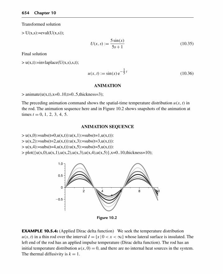
654 Chapter 10
Transformed solution
> U(x,s):=eval(U(x,s));
U(x, s) := 5 sin(x)
5s+1(10.35)
Final solution
> u(x,t):=invlaplace(U(x,s),s,t);
u(x, t) := sin(x) e−15 t (10.36)
ANIMATION
> animate(u(x,t),x=0..10,t=0..5,thickness=3);
The preceding animation command shows the spatial-time temperature distribution u(x, t) inthe rod. The animation sequence here and in Figure 10.2 shows snapshots of the animation attimes t = 0, 1, 2, 3, 4, 5.
ANIMATION SEQUENCE
> u(x,0):=subs(t=0,u(x,t)):u(x,1):=subs(t=1,u(x,t)):> u(x,2):=subs(t=2,u(x,t)):u(x,3):=subs(t=3,u(x,t)):> u(x,4):=subs(t=4,u(x,t)):u(x,5):=subs(t=5,u(x,t)):> plot({u(x,0),u(x,1),u(x,2),u(x,3),u(x,4),u(x,5)},x=0..10,thickness=10);
x2 4 6 8 10
20.5
0
0.5
1.0
Figure 10.2
EXAMPLE 10.5.4: (Applied Dirac delta function) We seek the temperature distributionu(x, t) in a thin rod over the interval I = {x |0 < x < ∞} whose lateral surface is insulated. Theleft end of the rod has an applied impulse temperature (Dirac delta function). The rod has aninitial temperature distribution u(x,0) = 0, and there are no internal heat sources in the system.The thermal diffusivity is k = 1.

Laplace Transform Methods for Partial Differential Equations 655
SOLUTION: The diffusion partial differential equation is
∂
∂tu(x, t) = k
(∂2
∂x2u(x, t)
)
The boundary conditions are
u(0, t) = δ(t) and u(∞, t) < ∞
The initial condition is
u(x,0) = 0
The Laplace transformed equation reads
∂2
∂x2U(x, s)− sU(x, s)
k= −f(x)
k
Here, U(x, s) is the Laplace transform of u(x, t) with respect to t. The transformed boundaryconditions are
U(0, s) = Q(s) and U(∞, s) < ∞
Assignment of system parameters
> restart:with(plots):with(inttrans):k:=1:q(t):=Dirac(t):f(x):=0:
Transformed equation in x reads
> diff(U(x,s),x,x)−(1/k)*s*U(x,s)=−1/k*f(x);
∂2
∂x2U(x, s)− sU(x, s) = 0 (10.37)
Transformed boundary conditions
> Q(s):=Int(q(t)*exp(−s*t),t=0..infinity);
Q(s) :=∞∫
0
Dirac(t) e−stdt (10.38)
> Q(s):=laplace(q(t),t,s);
Q(s) := 1 (10.39)

656 Chapter 10
General solution for U(x, s)
> assume(x>0):U(x,s):=C1(s)*exp(−sqrt(s/k)*x)+C2(s)*exp(sqrt(s/k)*x);
U(x∼, s) := C1(s) e−√s x∼ +C2(s) e
√s x∼ (10.40)
Substituting the boundary conditions at x = 0 and as x approaches infinity, for Re{s} > 0,we get
> C2(s):=0;
C2(s) := 0 (10.41)
> eq:=Q(s)=eval(subs(x=0,U(x,s)));
eq := 1 = C1(s) (10.42)
> C1(s):=solve(eq,C1(s));
C1(s) := 1 (10.43)
Transformed solution
> U(x,s):=eval(U(x,s));
U(x∼, s) := e−√s x∼ (10.44)
Solution is the inverse Laplace of U(x, s)
> u(x,t):=invlaplace(U(x,s),s,t);
u(x∼, t) := 1
2
x∼ e−14
x∼2
t√π t3/2
(10.45)
ANIMATION
> animate(u(x,t),x=0..10,t=0..5,thickness=3);
The preceding animation command shows the spatial-time temperature distribution u(x, t) inthe rod. The animation sequence here and in Figure 10.3 shows snapshots of the animation attimes t = 1/2, 1, 2, 3, 4, 5.
ANIMATION SEQUENCE
> u(x,0):=subs(t=1/2,u(x,t)):u(x,1):=subs(t=1,u(x,t)):> u(x,2):=subs(t=2,u(x,t)):u(x,3):=subs(t=3,u(x,t)):> u(x,4):=subs(t=4,u(x,t)):u(x,5):=subs(t=5,u(x,t)):> plot({u(x,0),u(x,1),u(x,2),u(x,3),u(x,4),u(x,5)},x=0..10,thickness=10);

Laplace Transform Methods for Partial Differential Equations 657
x~0 2 4 6 8 10
0
0.1
0.2
0.3
0.4
Figure 10.3
EXAMPLE 10.5.5: (End of rod with temperature constraint) We seek the temperaturedistribution u(x, t) in a thin rod over the interval I = {x |0 < x < ∞} whose lateral surface isinsulated. The left end of the rod is constrained at a varying temperature q(t) given following,and the rod has an initial temperature distribution u(x,0) = 0. There is no heat source in thesystem and the thermal diffusivity of the rod is k = 1/50.
SOLUTION: The diffusion partial differential equation is
∂
∂tu(x, t) = k
(∂2
∂x2u(x, t)
)
The boundary conditions are
u(0, t) = 1√t
and u(∞, t) < ∞
The initial condition is
u(x,0) = 0
The Laplace transformed equation reads
∂2
∂x2U(x, s)− sU(x, s)
k= −f(x)
k
Here, U(x, s) is the Laplace transform of u(x, t) with respect to t. The transformed boundaryconditions are
U(0, s) = Q(s) and U(∞, s) < ∞Assignment of system parameters
> restart:with(plots):with(inttrans):k:=1/50:q(t):=1/sqrt(t):f(x):=0:

658 Chapter 10
Transformed equation in x reads
> diff(U(x,s),x,x)−(1/k)*s*U(x,s)=−1/k*f(x);
∂2
∂x2U(x, s)−50sU(x, s) = 0 (10.46)
Transformed boundary conditions
> Q(s):=Int(q(t)*exp(−s*t),t=0..infinity);
Q(s) :=∞∫
0
e−st
√t
dt (10.47)
> Q(s):=laplace(q(t),t,s);
Q(s) :=√
π
s(10.48)
General solution for U(x, s)
> assume(x>0):U(x,s):=C1(s)*exp(−sqrt(s/k)*x)+C2(s)*exp(sqrt(s/k)*x);
U(x∼, s) := C1(s) e−5√
2√
s x∼ +C2(s) e5√
2√
s x∼ (10.49)
Substituting the boundary conditions at x = 0 and as x approaches infinity, for Re{s} > 0,we get
> C2(s):=0;
C2(s) := 0 (10.50)
> eq:=Q(s)=eval(subs(x=0,U(x,s)));
eq :=√
π
s= C1(s) (10.51)
> C1(s):=solve(eq,C1(s));
C1(s) :=√
π
s(10.52)
Transformed solution
> U(x,s):=eval(U(x,s));
U(x∼, s) :=√
π
se−5
√2√
sx∼ (10.53)

Laplace Transform Methods for Partial Differential Equations 659
Solution is the inverse Laplace of U(x, s)
> u(x,t):=invlaplace(U(x,s),s,t);
u(x∼, t) := e−252
x∼2
t√t
(10.54)
ANIMATION
> animate(u(x,t),x=0..1,t=0..5,thickness=3);
The preceding animation command shows the spatial-time temperature distribution u(x, t) inthe rod. The animation sequence here and in Figure 10.4 shows snapshots of the animation attimes t = 1/5, 1,2,3,4,5.
ANIMATION SEQUENCE
>u(x,0):=subs(t=1/5,u(x,t)):u(x,1):=subs(t=1,u(x,t)):> u(x,2):=subs(t=2,u(x,t)):u(x,3):=subs(t=3,u(x,t)):> u(x,4):=subs(t=4,u(x,t)):u(x,5):=subs(t=5,u(x,t)):> plot({u(x,0),u(x,1),u(x,2),u(x,3),u(x,4),u(x,5)},x=0..10,thickness=10);
x~0 0.2 0.4 0.6 0.8 1
0
0.5
1.0
1.5
2.0
Figure 10.4
EXAMPLE 10.5.6: (Input heat flux) We seek the temperature distribution u(x, t) in a thin rodover the semi-infinite interval I = {x |0 < x < ∞} whose lateral surface is insulated. The leftend of the rod has an input heat flux q(t) given following, and the initial temperaturedistribution is 0. There is no internal heat source in the system, and the thermal diffusivity isk = 1/20. We want to solve this problem using convolution methods.
SOLUTION: The diffusion partial differential equation is
∂
∂tu(x, t) = k
(∂2
∂x2u(x, t)
)

660 Chapter 10
The boundary conditions are
ux(0, t) = −10 and u(∞, t) < ∞The initial condition is
u(x,0) = 0
The Laplace transformed equation reads
∂2
∂x2U(x, s)− sU(x, s)
k= −f(x)
k
Here, U(x, s) is the Laplace transform of u(x, t) with respect to t. The transformed boundaryconditions are
∂
∂xU(0, s) = Q(s) and U(∞, s) < ∞
Assignment of system parameters
> restart:with(plots):with(inttrans):k:=1/20:q(t):=−10:f(x):=0:
Transformed equation in x reads
> diff(U(x,s),x,x)−(1/k)*s*U(x,s)=−1/k*f(x);
∂2
∂x2U(x, s)−20sU(x, s) = 0 (10.55)
Transformed boundary conditions
> Q(s)=Int(q(t)*exp(−s*t),t=0..infinity);
Q(s) =∞∫
0
(−10 e−st)
dt (10.56)
> Q(s):=laplace(q(t),t,s);
Q(s) := −10
s(10.57)
General solution for U(x, s)
> assume(x>0):U(x,s):=C1(s)*exp(−sqrt(s/k)*x)+C2(s)*exp(sqrt(s/k)*x);
U(x∼, s) := C1(s) e−2√
5√
s x∼ +C2(s) e2√
5√
s x∼ (10.58)

Laplace Transform Methods for Partial Differential Equations 661
Substituting the boundary conditions at x = 0 and as x approaches infinity, for Re{s} > 0, we get
> C2(s):=0;
C2(s) := 0 (10.59)
> eq:=Q(s)=eval(subs(x=0,diff(U(x,s),x)));
eq := −10
s= −2C1(s)
√5√
s (10.60)
> C1(s):=solve(eq,C1(s));
C1(s) :=√
5
s3/2(10.61)
Transformed solution
> U(x,s):=eval(U(x,s));
U(x∼, s) :=√
5 e−2√
5√
s x∼s3/2
(10.62)
Convolution partition
> U1(x,s):=U(x,s)*s;
U1(x∼, s) :=√
5 e−2√
5√
s x∼√
s(10.63)
> U2(x,s):=1/s;
U2(x∼, s) := 1
s(10.64)
> u1(x,t):=invlaplace(U1(x,s),s,t);u1(x,tau):=subs(t=tau,u1(x,t)):
u1(x∼, t) :=√
5 e− 5x∼2t√
πt(10.65)
> u2(x,t):=simplify(invlaplace(U2(x,s),s,t));u2(x,t−tau):=subs(t=t−tau,u2(x,t)):
u2(x ∼, t) := 1 (10.66)
Convolution integral solution
> u(x,t):=Int(u1(x,tau)*u2(x,t−tau),tau=0..t);u(x,t):=simplify(value(%)):
u(x∼, t) :=t∫
0
√5 e− 5x∼2
τ√πτ
dτ (10.67)
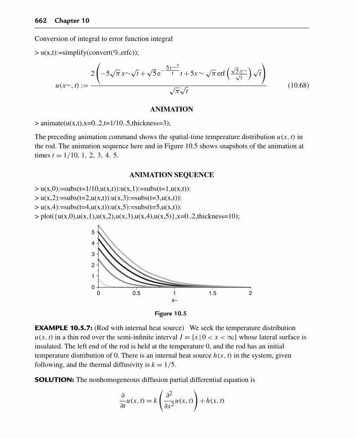
662 Chapter 10
Conversion of integral to error function integral
> u(x,t):=simplify(convert(%,erfc));
u(x∼, t) :=2
(−5
√π x∼√
t +√5 e−5x∼2
t t +5x∼ √π erf
(√5x∼√
t
)√t
)√
π√
t(10.68)
ANIMATION
> animate(u(x,t),x=0..2,t=1/10..5,thickness=3);
The preceding animation command shows the spatial-time temperature distribution u(x, t) inthe rod. The animation sequence here and in Figure 10.5 shows snapshots of the animation attimes t = 1/10, 1, 2, 3, 4, 5.
ANIMATION SEQUENCE
> u(x,0):=subs(t=1/10,u(x,t)):u(x,1):=subs(t=1,u(x,t)):> u(x,2):=subs(t=2,u(x,t)):u(x,3):=subs(t=3,u(x,t)):> u(x,4):=subs(t=4,u(x,t)):u(x,5):=subs(t=5,u(x,t)):> plot({u(x,0),u(x,1),u(x,2),u(x,3),u(x,4),u(x,5)},x=0..2,thickness=10);
x~0 0.5 1 1.5 2
0
1
2
3
4
5
Figure 10.5
EXAMPLE 10.5.7: (Rod with internal heat source) We seek the temperature distributionu(x, t) in a thin rod over the semi-infinite interval I = {x |0 < x < ∞} whose lateral surface isinsulated. The left end of the rod is held at the temperature 0, and the rod has an initialtemperature distribution of 0. There is an internal heat source h(x, t) in the system, givenfollowing, and the thermal diffusivity is k = 1/5.
SOLUTION: The nonhomogeneous diffusion partial differential equation is
∂
∂tu(x, t) = k
(∂2
∂x2u(x, t)
)+h(x, t)
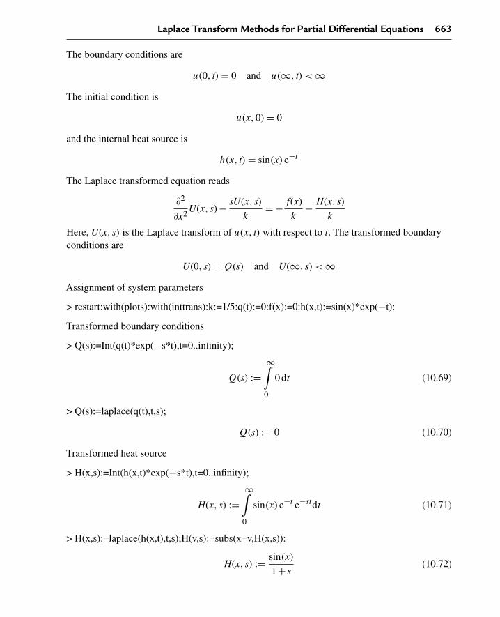
Laplace Transform Methods for Partial Differential Equations 663
The boundary conditions are
u(0, t) = 0 and u(∞, t) < ∞The initial condition is
u(x,0) = 0
and the internal heat source is
h(x, t) = sin(x) e−t
The Laplace transformed equation reads
∂2
∂x2U(x, s)− sU(x, s)
k= −f(x)
k− H(x, s)
k
Here, U(x, s) is the Laplace transform of u(x, t) with respect to t. The transformed boundaryconditions are
U(0, s) = Q(s) and U(∞, s) < ∞Assignment of system parameters
> restart:with(plots):with(inttrans):k:=1/5:q(t):=0:f(x):=0:h(x,t):=sin(x)*exp(−t):
Transformed boundary conditions
> Q(s):=Int(q(t)*exp(−s*t),t=0..infinity);
Q(s) :=∞∫
0
0 dt (10.69)
> Q(s):=laplace(q(t),t,s);
Q(s) := 0 (10.70)
Transformed heat source
> H(x,s):=Int(h(x,t)*exp(−s*t),t=0..infinity);
H(x, s) :=∞∫
0
sin(x) e−t e−stdt (10.71)
> H(x,s):=laplace(h(x,t),t,s);H(v,s):=subs(x=v,H(x,s)):
H(x, s) := sin(x)
1+ s(10.72)

664 Chapter 10
Transformed equation in x reads
> diff(U(x,s),x,x)−(1/k)*s*U(x,s)=−f(x)/k−H(x,s)/k;
∂2
∂x2U(x, s)−5sU(x, s) = −5 sin(x)
1+ s(10.73)
Basis vectors to x equation
> phi[1](x,s):=exp(−sqrt(s/k)*x);phi[1](v,s):=subs(x=v,phi[1](x,s)):phi[2](x,s):=exp(sqrt(s/k)*x);phi[2](v,s):=subs(x=v,phi[2](x,s)):
φ1(x, s) : = e−√5√
s x
φ2(x, s) : = e√
5√
s x (10.74)
Evaluation of Wronskian
> W(phi[1](v,s),phi[2](v,s)):=simplify(phi[1](v,s)*diff(phi[2](v,s),v)−phi[2](v,s)*diff(phi[1](v,s),v));
W(
e−√5√
s v, e√
5√
s v)
:= 2√
5√
s (10.75)
Evaluation of Green’s function
> G(x,v,s):=(phi[1](v,s)*phi[2](x,s)−phi[1](x,s)*phi[2](v,s))/W(phi[1](v,s),phi[2](v,s));
G(x, v, s) := 1
10
(e−√
5√
s v e√
5√
s x − e−√5√
s x e√
5√
s v)√
5√
s(10.76)
Particular solution to the transformed equation
> Up(x,s):=−Int(G(x,v,s)*H(v,s)/k,v);Up(x,s):=value(%):
Up(x, s) := −⎛⎝∫
1
2
(e−√
5√
s ve√
5√
s x − e−√5√
s x e√
5√
s v)√
5 sin(v)√
s(1+ s)dv
⎞⎠ (10.77)
> Up(x,s):=simplify(subs(v=x,%));
Up(x, s) := 5 sin(x)
(1+ s)(5s+1)(10.78)

Laplace Transform Methods for Partial Differential Equations 665
General solution
> U(x,s):=C1(s)*phi[1](x,s)+C2(s)*phi[2](x,s)+Up(x,s);
U(x, s) := C1(s) e−√5√
s x +C2(s) e√
5√
s x + 5 sin(x)
(1+ s)(5s+1)(10.79)
Substituting the boundary conditions at x = 0 and as x approaches infinity, for Re{s} > 0,we get
> C2(s):=0;
C2(s) := 0 (10.80)
> eq:=Q(s)=eval(subs(x=0,U(x,s)));
eq := 0 = C1(s) (10.81)
> C1(s):=solve(eq,C1(s));
C1(s) := 0 (10.82)
Transformed solution
> U(x,s):=eval(U(x,s));
U(x, s) := 5 sin(x)
(1+ s)(5s+1)(10.83)
Final solution
> u(x,t):=invlaplace(U(x,s),s,t);
u(x, t) := 5
2sin(x) e− 3
5 t sinh
(2
5t
)(10.84)
ANIMATION
> animate(u(x,t),x=0..10,t=0..5,thickness=3);
The preceding animation command shows the spatial-time temperature distribution u(x, t) inthe rod. The animation sequence here and in Figure 10.6 shows snapshots of the animation attimes t = 0, 1,2,3,4,5.
ANIMATION SEQUENCE
> u(x,0):=subs(t=0,u(x,t)):u(x,1):=subs(t=1,u(x,t)):> u(x,2):=subs(t=2,u(x,t)):u(x,3):=subs(t=3,u(x,t)):> u(x,4):=subs(t=4,u(x,t)):u(x,5):=subs(t=5,u(x,t)):> plot({u(x,0),u(x,1),u(x,2),u(x,3),u(x,4),u(x,5)},x=0..10,thickness=10);

666 Chapter 10
x
0.6
0.4
0.2
0
20.22 4 86 10
20.4
20.6
Figure 10.6
10.6 Laplace Transform Procedures on theWave Equation
We consider the nonhomogeneous partial differential equation for wave phenomena in onespatial dimension in rectangular coordinates as given here:
∂2
∂t2u(x, t) = c2
(∂2
∂x2u(x, t)
)+h(x, t)
with the two initial conditions
u(x,0) = f(x) and ut(x,0) = g(x)
The term h(x, t) accounts for any external sources in the system, f(x) denotes the initialdisplacment distribution, and g(x) denotes the initial speed distribution. We assume that thereis no damping in the system.
In evaluating the Laplace transform of terms in the preceding equation, we have to contendwith taking improper integrals with respect to t of functions that are dependent on both x and t.We denote the Laplace transform of u(x, t) with respect to the time variable t by the capitalletter representation as shown:
∞∫0
u(x, t) e−stdt = U(x, s)
Proceeding formally with the evaluation of transforms of the derivative terms in the givenpartial differential equation, we get
∞∫0
(∂2
∂t2u(x, t)
)e−stdt = s2U(x, s)− su(x,0)−ut(x,0)
Laplace Transform Methods for Partial Differential Equations 667
In the preceding, U(x, s) denotes the Laplace transform of u(x, t) with respect to t; u(x,0)
denotes the initial value of u(x, t); and ut(x,0) denotes the initial speed.
Proceeding formally, in evaluating the transforms of the partial derivative terms with respect tothe spatial variable x, we get
∞∫0
(∂2
∂x2u(x, t)
)e−stdt = ∂2
∂x2U(x, s)
This operation assumes that we could interchange the order of the differentiation operation,with respect to x, with the integration operation, with respect to t. The conditions for thevalidity of doing this are based on the uniform convergence of the improper integrals of thederivative terms.
Assuming the validity of all these given conditions, then the Laplace transform of the wavepartial differential equation gives us
∂2
∂x2U(x, s)− s2U(x, s)
c2= −sf(x)
c2− g(x)
c2− H(x, s)
c2
Here, H(x, s) is the Laplace transform of the source term given as
H(x, s) =∞∫
0
h(x, t) e−stdt
The preceding differential equation is an ordinary second-order nonhomogeneous differentialequation in the single spatial variable x. We investigated the solutions for this equation inChapter 1. The solutions are, of course, dependent on the spatial boundary conditions on theproblem.
We now implement the Laplace transform method to evaluate solutions to the wave equationover semi-infinite domains with respect to the spatial variable x. We focus on those types ofproblems that may or may not have nonhomogeneous boundary conditions—those problemsthat cannot ordinarily be solved using Fourier transform methods as covered in Chapter 9.Further, we do not consider using Laplace transform methods for wave problems over finitedomains here because eigenfunction expansion methods, as used in Chapters 4, 7, and 8, aremore effective.
In general, we consider time-dependent boundary conditions that are nonhomogeneous atx = 0 and are bounded as x approaches infinity; that is,
κ1u(0, t)+κ2ux(0, t) = q(t)
and
u(∞, t) < ∞

668 Chapter 10
The transform of these boundary conditions yields
κ1U(0, s)+κ2
(∂
∂xU(0, s)
)= Q(s)
and
U(∞, s) < ∞where the term ∂
∂xU(0, s) is understood to be the x-dependent derivative of U(x, s) evaluated atx = 0 and Q(s) is the Laplace transform of q(t) as shown here:
Q(s) =∞∫
0
q(t) e−stdt
To develop the general solution to the given nonhomogeneous differential equation, we use themethod of variation of parameters as outlined in Chapter 1 whereby we must first considerfinding a set of basis vectors for the following corresponding homogeneous differentialequation:
∂2
∂x2U(x, s)− s2U(x, s)
c2= 0
A set of two basis vectors is
φ1(x, s) = e− sxc
and
φ2(x, s) = esxc
From the two basis vectors, we are able to generate the second-order Green’s function
G(x, v, s) = φ1(v, s)φ2(x, s)−φ1(x, s)φ2(v, s)
W(φ1(v, s),φ2(v, s))
where the denominator term is the familiar Wronskian, which, for the basis vectors shown, isevaluated to be
W(φ1(v, s),φ2(v, s)) = 2 s
c
Thus, from the method of varaiation of parameters, the particular solution to thenonhomogeneous ordinary differential equation in x is
Up(x, s) = −(∫
G(x, v, s)(sf(v)+g(v)+H(v, s))
c2dv
)

Laplace Transform Methods for Partial Differential Equations 669
The general solution to the x-dependent differential equation is the sum of the complementarysolution and the particular solution preceding. Combining the two solutions, we get the generalsolution for the transform U(x, s):
U(x, s) = C1(s) e− sxc +C2(s) e
sxc −
(∫G(x, v, s)(sf(v)+g(v)+H(v, s))
c2dv
)
The arbitrary coefficients C1(s) and C2(s) are determined from the boundary conditions for theproblem. The final solution to our problem is the inverse Laplace transform of U(x, s). We nowdemonstrate these concepts by solving the illustrative problem of a string falling under its ownweight.
DEMONSTRATION: We seek the wave amplitude u(x, t) for transverse wave motion along ataut string over the semi-infinite interval I = {x |0 < x < ∞}. The left end of the string is heldsecure. The string has zero initial displacement and initial speed. An external force due togravity (acceleration = −980 cm/sec2) is acting uniformly on the string, and the wave speedconstant is c = 2. There is no damping in the system.
SOLUTION: The nonhomogeneous wave partial differential equation for the string is
∂2
∂t2u(x, t) = 4
(∂2
∂x2u(x, t)
)−980
Because the string is secure at the left end and we require the solution to be finite as x
approaches infinity, the boundary conditions are
u(0, t) = 0 and u(∞, t) < ∞The string is initially at rest, and it has no initial displacement; thus, the initial conditions are
u(x,0) = 0 and ut(x,0) = 0
The Laplace transform, with respect to t, of the partial differential equation yields the ordinarynonhomogeneous differential equation for the transformed variable U(x, s), which reads
∂2
∂x2U(x, s)− s2U(x, s)
4= 245
s
The corresponding transformed boundary conditions are
U(0, s) = 0 and U(∞, s) < ∞From Section 1.5, a set of basis vectors for the x-dependent differential equation is
φ1(x, s) = e− sx2

670 Chapter 10
and
φ2(x, s) = esx2
The Wronskian for this basis is
W
(e− sv
2 , esv2
)= s
From Section 1.7, the corresponding second-order Green’s function is
G(x, v, s) = e− sv2 e
sx2 − e− sx
2 esv2
s
The particular solution to the nonhomogeneous differential equation, for the transformedvariable U(x, s), is given as the Green’s function integral
Up(x, s) =∫ 245
(e− sv
2 esx2 − e− sx
2 esv2
)s2
dv
which is evaluated to be
Up(x, s) = −980
s3
Thus, the general solution to the ordinary differential equation for the transformed solutionU(x, s) is
U(x, s) = C1(s) e− sx2 +C2(s) e
sx2 − 980
s3(10.85)
Here, C1(s) and C2(s) are arbitrary constants that are determined from the boundaryconditions. Substituting the boundary condition at x = 0 and as x approaches infinity, forRe{s} > 0, we get the transformed solution
U(x, s) = 980 e− sx2
s3− 980
s3
Evaluation of the inverse Laplace transform yields the spatial- and time-dependent solutionu(x, t) for the falling string:
u(x, t) = 490H(t − x
2
)(t − x
2
)2 −490 t2
where H(t − x
2
)denotes the translated Heaviside function. The details for the development of
this solution and the graphics are given later in one of the Maple worksheet examples.

Laplace Transform Methods for Partial Differential Equations 671
10.7 Example Laplace Transform Problems for theWave Equation
We now look at some specific applications of the Laplace transform in evaluating solutions tothe wave equation over semi-infinite domains with respect to the spatial variable x. We focuson those types of problems that have nonhomogeneous boundary conditions—problems thatcannot ordinarily be solved using Fourier transform methods as covered in Chapter 9.
EXAMPLE 10.7.1: (The vibrating string) We seek the wave amplitude u(x, t) for transversewave motion along a taut string over the semi-infinite interval I = {x |0 < x < ∞}. The leftend of the string is constrained to move in accordance with the sinusoidal function q(t) givenfollowing. The string has an initial displacement distribution f(x) and an initial speeddistribution g(x). There is no external source function, and there is no damping in the system.The wave speed is c = 2.
SOLUTION: The wave partial differential equation is
∂2
∂t2u(x, t) = c2
(∂2
∂x2u(x, t)
)
The boundary conditions are
u(0, t) = sin(t) and u(∞, t) < ∞The initial conditions are
u(x,0) = 0 and ut(x,0) = 0
The Laplace transformed equation reads
∂2
∂x2U(x, s)− s2U(x, s)
c2= −sf(x)
c2− g(x)
c2
Here, U(x, s) is the Laplace transform of u(x, t) with respect to t. The transformed boundaryconditions are
U(0, s) = Q(s) and U(∞, s) < ∞Assignment of system parameters
> restart:with(plots):with(inttrans):c:=2:q(t):=sin(t):f(x):=0:g(x):=0:
Transformed equation in x reads
> diff(U(x,s),x,x)−sˆ2/cˆ2*U(x,s)=−s*f(x)/cˆ2−g(x)/cˆ2;
∂2
∂x2U(x, s)− 1
4s2U(x, s) = 0 (10.86)

672 Chapter 10
Transformed boundary conditions
> Q(s):=Int(q(t)*exp(−s*t),t=0..infinity);
Q(s) :=∞∫
0
sin(t) e−s tdt (10.87)
> Q(s):=laplace(q(t),t,s);
Q(s) := 1
s2 +1(10.88)
General solution for U(x, s)
> assume(x>0):U(x,s):=C1(s)*exp(−s/c*x)+C2(s)*exp(s/c*x);
U(x∼, s) := C1(s) e−12 sx∼ +C2(s) e
12 sx∼ (10.89)
Substituting the boundary conditions at x = 0 and as x approaches infinity, for Re{s} > 0,we get
> C2(s):=0;
C2(s) := 0 (10.90)
> eq:=Q(s)=eval(subs(x=0,U(x,s)));
eq := 1
s2 +1= C1(s) (10.91)
> C1(s):=solve(eq, C1(s));
C1(s) := 1
s2 +1(10.92)
Transformed solution
> U(x,s):=eval(U(x,s));
U(x∼, s) := e−12 sx∼
s2 +1(10.93)
Solution is the inverse Laplace of U(x, s)
> u(x,t):=invlaplace(U(x,s),s,t);
u(x∼, t) := Heaviside
(t − 1
2x∼
)sin
(t − 1
2x∼
)(10.94)

Laplace Transform Methods for Partial Differential Equations 673
ANIMATION
> animate(u(x,t),x=0..10,t=0..10,thickness=3);
The preceding animation command shows the spatial-time wave amplitude distribution u(x, t)
on the string. The animation sequence here and in Figure 10.7 shows snapshots of theanimation at times t = 0, 1, 2, 3, 4, 5.
ANIMATION SEQUENCE
> u(x,0):=subs(t=0,u(x,t)):u(x,1):=subs(t=1,u(x,t)):> u(x,2):=subs(t=2,u(x,t)):u(x,3):=subs(t=3,u(x,t)):> u(x,4):=subs(t=4,u(x,t)):u(x,5):=subs(t=5,u(x,t)):> plot({u(x,0),u(x,1),u(x,2),u(x,3),u(x,4),u(x,5)},x=0..10,thickness=10);
x~
1.0
0.5
02 4 6 8 10
20.5
Figure 10.7
EXAMPLE 10.7.2: (String falling under its own weight) We seek the wave amplitudeu(x, t) for transverse wave motion along a taut string over the semi-infinite intervalI = {x |0 < x < ∞}. The left end of the string is held fixed. The string has the initialdisplacement distribution f(x) = 0 and the initial speed distribution g(x) = 0. An externalforce due to gravity (acceleration = −980 cm/sec2) is acting uniformly on the string, and weassume no damping in the system. The wave speed is c = 2.
SOLUTION: The nonhomogeneous wave partial differential equation is
∂2
∂t2u(x, t) = c2
(∂2
∂x2u(x, t)
)+h(x, t)
The boundary conditions are
u(0, t) = 0 and u(∞, t) < ∞
674 Chapter 10
The initial conditions are
u(x,0) = 0 and ut(x,0) = 0
The Laplace transformed equation reads
∂2
∂x2U(x, s)− s2U(x, s)
c2= −sf(x)
c2− g(x)
c2− H(x, s)
c2
Here, U(x, s) is the Laplace transform of u(x, t) with respect to t. The transformed boundaryconditions are
U(0, s) = Q(s) and U(∞, s) < ∞Assignment of system parameters
> restart:with(plots):with(inttrans):c:=2:q(t):=0:f(x):=0:f(v):=subs(x=v,f(x)):g(x):=0:g(v):=subs(x=v,g(x)):h(x,t):=−980:
Transformed equation in x reads
> diff(U(x,s),x,x)−sˆ2/cˆ2*U(x,s)=−s*f(x)/cˆ2−g(x)/cˆ2−H(x,s)/cˆ2;
∂2
∂x2U(x, s)− 1
4s2U(x, s) = −1
4H(x, s) (10.95)
Transformed boundary conditions
> Q(s):=Int(q(t)*exp(−s*t),t=0..infinity);
Q(s) :=∞∫
0
0 dt (10.96)
> Q(s):=value(%);
Q(s) := 0 (10.97)
Transformed source term
> H(x,s):=Int(h(x,t)*exp(−s*t),t=0..infinity);
H(x, s) :=∞∫
0
(−980 e−st) dt (10.98)
> H(x,s):=laplace(h(x,t),t,s);H(v,s):=subs(x=v,H(x,s)):
H(x, s) := −980
s(10.99)

Laplace Transform Methods for Partial Differential Equations 675
Basis vectors
> assume(x>0):phi[1](x,s):=exp(−s/c*x);phi[1](v,s):=subs(x=v,phi[1](x,s)):phi[2](x,s):=exp(s/c*x);phi[2](v,s):=subs(x=v,phi[2](x,s)):
φ1(x∼, s) : = e−12 sx∼
φ2(x∼, s) : = e12 sx∼ (10.100)
Evaluation of the Wronskian
> W(phi[1](v,s),phi[2](v,s)):=simplify(phi[1](v,s)*diff(phi[2](v,s),v)−phi[2](v,s)*diff(phi[1](v,s),v));
W
(e− 1
2 sv, e12 sv
):= s (10.101)
Evaluation of the Green’s function
> G(x,v,s):=(phi[1](v,s)*phi[2](x,s)−phi[1](x,s)*phi[2](v,s))/W(phi[1](v,s),phi[2](v,s));
G(x∼, v, s) := e−12 sv e
12 sx∼ − e−1
2 sx∼ e12 sv
s(10.102)
Particular solution
> Up(x,s):=−Int(G(x,v,s)*(s*f(v)+g(v)+H(v,s))/cˆ2,v);
Up(x∼, s) := −
⎛⎜⎜⎝∫ ⎛
⎜⎜⎝−245
(e−1
2 sv e12 sx∼ − e−1
2 sx∼ e12 sv
)s2
⎞⎟⎟⎠dv
⎞⎟⎟⎠ (10.103)
> Up(x,s):=simplify(subs(v=x,value(%)));
Up(x∼, s) := −980
s3(10.104)
General solution
> U(x,s):=C1(s)*exp(−s/c*x)+C2(s)*exp(s/c*x)+Up(x,s);
U(x∼, s) := C1(s) e−12 sx∼ +C2(s) e
12 sx∼ − 980
s3(10.105)

676 Chapter 10
Substituting the boundary conditions at x = 0 and as x approaches infinity, for Re{s} > 0,we get
> C2(s):=0;
C2(s) := 0 (10.106)
> eq:=Q(s)=eval(subs(x=0,U(x,s)));
eq := 0 = C1(s)− 980
s3(10.107)
> C1(s):=solve(eq,C1(s));
C1(s) := 980
s3(10.108)
Transformed solution for U(x, s)
> U(x,s):=eval(U(x,s));
U(x∼, s) := 980 e−12 sx∼
s3− 980
s3(10.109)
Solution is the inverse Laplace of U(x, s)
> u(x,t):=invlaplace(U(x,s),s,t);
u(x∼, t) := −490 t2 + 245
2Heaviside
(t − 1
2x∼
)(2 t −x∼)2 (10.110)
ANIMATION
> animate(u(x,t),x=0..12,t=0..5,thickness=3);
The preceding animation command shows the spatial-time wave amplitude distribution u(x, t)
on the string. The animation sequence here and in Figure 10.8 shows snapshots of theanimation at times t = 0, 1, 2, 3, 4, 5.
ANIMATION SEQUENCE
> u(x,0):=subs(t=0,u(x,t)):u(x,1):=subs(t=1,u(x,t)):> u(x,2):=subs(t=2,u(x,t)):u(x,3):=subs(t=3,u(x,t)):> u(x,4):=subs(t=4,u(x,t)):u(x,5):=subs(t=5,u(x,t)):> plot({u(x,0),u(x,1),u(x,2),u(x,3),u(x,4),u(x,5)},x=0..12,thickness=10);

Laplace Transform Methods for Partial Differential Equations 677
02 4 6 8 10 12
22000
24000
26000
28000
210000
212000
x~
Figure 10.8
EXAMPLE 10.7.3: (Longitudinal vibrations in a bar) We seek the wave amplitude forlongitudinal wave motion in a bar over the semi-infinite interval I = {x |0 < x < ∞}. The leftend of the bar is experiencing an applied stress force q(t) (the Young’s modulus E = 1). Eachcross section of the bar has the initial displacement distribution f(x) = 0 and the initial speeddistribution g(x) = 0. There are no external forces acting upon the bar, and there is nodamping. The wave speed is c = 2.
SOLUTION: The wave partial differential equation is
∂2
∂t2u(x, t) = c2
(∂2
∂x2u(x, t)
)
The boundary conditions are
ux(0, t) = −cos(t) and u(∞, t) < ∞The initial conditions are
u(x,0) = 0 and ut(x,0) = 0
The Laplace transformed equation reads
∂2
∂x2U(x, s)− s2U(x, s)
c2= −sf(x)
c2− g(x)
c2
Here, U(x, s) is the Laplace transform of u(x, t) with respect to t. The transformed boundaryconditions are
∂
∂xU(0, s) = −Q(s) and U(∞, s) < ∞
Assignment of system parameters
> restart:with(plots):with(inttrans):c:=2:q(t):=cos(t):f(x):=0:g(x):=0:

678 Chapter 10
Transformed equation in x reads
> diff(U(x,s),x,x)−sˆ2/cˆ2*U(x,s)=−s*f(x)/cˆ2−g(x)/cˆ2;
∂2
∂x2U(x, s)− 1
4s2U(x, s) = 0 (10.111)
Transformed boundary conditions
> Q(s):=Int(q(t)*exp(−s*t),t=0..infinity);
Q(s) :=∞∫
0
cos(t) e−stdt (10.112)
> Q(s):=laplace(q(t),t,s);
Q(s) := s
s2 +1(10.113)
General solution for U(x, s)
> assume(x>0):U(x,s):=C1(s)*exp(−s/c*x)+C2(s)*exp(s/c*x);
U(x∼, s) := C1(s) e−12 sx∼ +C2(s) e
12 sx∼ (10.114)
Substituting the boundary conditions at x = 0 and as x approaches infinity, for Re{s} > 0, we get
> C2(s):=0;
C2(s) := 0 (10.115)
> eq:=Q(s)=−eval(subs(x=0,diff(U(x,s),x)));
eq := s
s2 +1= 1
2C1(s)s (10.116)
> C1(s):=solve(eq,C1(s));
C1(s) := 2
s2 +1(10.117)
Transformed solution
> U(x,s):=eval(U(x,s));
U(x∼, s) := 2 e−12 sx∼
s2 +1(10.118)

Laplace Transform Methods for Partial Differential Equations 679
Solution is the inverse Laplace of U(x, s)
> u(x,t):=simplify(invlaplace(U(x,s),s,t));
u(x∼, t) := −2 sin
(t − 1
2x∼
)(−1+ Heaviside(x∼ −2 t)) (10.119)
ANIMATION
> animate(u(x,t),x=0..10,t=0..10,thickness=3);
The preceding animation command shows the spatial-time wave amplitude distribution u(x, t)
in the bar. The animation sequence here and in Figure 10.9 shows snapshots of the animation attimes t = 0, 1, 2, 3, 4, 5.
ANIMATION SEQUENCE
> u(x,0):=subs(t=0,u(x,t)):u(x,1):=subs(t=1,u(x,t)):> u(x,2):=subs(t=2,u(x,t)):u(x,3):=subs(t=3,u(x,t)):> u(x,4):=subs(t=4,u(x,t)):u(x,5):=subs(t=5,u(x,t)):> plot({u(x,0),u(x,1),u(x,2),u(x,3),u(x,4),u(x,5)}x=0..10,thickness=10);
x~
2
1
02 4 6 8 10
21
Figure 10.9
EXAMPLE 10.7.4: (Initially displaced string) We seek the wave amplitude u(x, t) fortransverse wave motion along a taut string over the semi-infinite interval I = {x |0 < x < ∞}.The left end of the string is held fixed. The string has the initial displacement distributionu(x,0) = f(x) given following, and the initial speed distribution g(x) = 0. There are noexternal forces acting upon the string, and there is no damping in the system. The wave speedis c = 1.
SOLUTION: The wave partial differential equation is
∂2
∂t2u(x, t) = c2
(∂2
∂x2u(x, t)
)

680 Chapter 10
The boundary conditions are
u(0, t) = 0 and u(∞, t) < ∞The initial conditions are
u(x,0) = x e−x and ut(x,0) = 0
The Laplace transformed equation reads
∂2
∂x2U(x, s)− s2U(x, s)
c2= −sf(x)
c2− g(x)
c2
Here, U(x, s) is the Laplace transform of u(x, t) with respect to t. The transformed boundaryconditions are
U(0, s) = Q(s) and U(∞, s) < ∞Assignment of system parameters
> restart:with(plots):with(inttrans):c:=1:q(t):=0:f(x):=x*exp(−x):f(v):=subs(x=v,f(x)):g(x):=0:g(v):=subs(x=v,g(x)):
Transformed equation in x reads
> diff(U(x,s),x,x)−sˆ2/cˆ2*U(x,s)=−s*f(x)/cˆ2−g(x)/cˆ2;
∂2
∂x2U(x, s)− s2U(x, s) = −sx e−x (10.120)
Transformed boundary conditions
> Q(s):=Int(q(t)*exp(−s*t),t=0..infinity);
Q(s) :=∞∫
0
0 dt (10.121)
> Q(s):=value(%);
Q(s) := 0 (10.122)
Basis vectors
> assume(x>0):phi[1](x,s):=exp(−s/c*x);phi[1](v,s):=subs(x=v,phi[1](x,s)):phi[2](x,s):=exp(s/c*x);phi[2](v,s):=subs(x=v,phi[2](x,s)):
φ1(x∼, s) : = e−sx∼
φ2(x∼, s) : = esx∼ (10.123)

Laplace Transform Methods for Partial Differential Equations 681
Evaluation of the Wronskian
> W(phi[1](v,s),phi[2](v,s)):=simplify(phi[1](v,s)*diff(phi[2](v,s),v)−phi[2](v,s)*diff(phi[1](v,s),v));
W( e−sv, esv) := 2s (10.124)
Evaluation of the Green’s function
> G(x,v,s):=(phi[1](v,s)*phi[2](x,s)−phi[1](x,s)*phi[2](v,s))/W(phi[1](v,s),phi[2](v,s));
G(x∼, v, s) := 1
2
e−sv esx∼ − e−sx∼ esv
s(10.125)
Particular solution
> Up(x,s):=−Int(G(x,v,s)*(s*f(v)+g(v))/cˆ2,v);
Up(x∼, s) := −(∫
1
2( e−sv esx∼ − e−sx∼ esv)v e−vdv
)(10.126)
> Up(x,s):=simplify(subs(v=x,value(%)));
Up(x∼, s) := e−x∼s(−x∼ −2+x∼ s2)
(1+ s)2(−1+ s)2(10.127)
General solution
> U(x,s):=C1(s)*exp(−s/c*x)+C2(s)*exp(s/c*x)+Up(x,s);
U(x∼, s) := C1(s) e−sx∼ +C2(s) esx∼ + e−x∼s(−x∼ −2+x∼s2)
(1+ s)2(−1+ s)2(10.128)
Substituting the boundary conditions at x = 0 and as x approaches infinity, for Re{s} > 0, we get
> C2(s):=0;
C2(s) := 0 (10.129)
> eq:=Q(s)=eval(subs(x=0,U(x,s)));
eq := 0 = C1(s)− 2s
(1+ s)2(−1+ s)2(10.130)
> C1(s):=solve(eq,C1(s));
C1(s) := 2s
1−2s2 + s4(10.131)

682 Chapter 10
Transformed solution for U(x, s)
> U(x,s):=eval(U(x,s));
U(x∼, s) := 2se−sx∼1−2s2 + s4
+ e−x∼s(−x∼ −2+x∼s2)
(1+ s)2(−1+ s)2(10.132)
Solution is the inverse Laplace of U(x, s)
> u(x,t):=invlaplace(U(x,s),s,t);
u(x∼, t) := Heaviside (t −x∼)(t −x∼) sinh(t −x∼)+ e−x∼ (x∼ cosh(t)− t sinh(t))
(10.133)
ANIMATION
> animate(u(x,t),x=0..12,t=0..5,thickness=3);
The preceding animation command shows the spatial-time amplitude distribution u(x, t) on thestring. The animation sequence here and in Figure 10.10 shows snapshots of the animation attimes t = 0, 1, 2, 3, 4, 5.
ANIMATION SEQUENCE
> u(x,0):=subs(t=0,u(x,t)):u(x,1):=subs(t=1,u(x,t)):> u(x,2):=subs(t=2,u(x,t)):u(x,3):=subs(t=3,u(x,t)):> u(x,4):=subs(t=4,u(x,t)):u(x,5):=subs(t=5,u(x,t)):> plot({u(x,0),u(x,1),u(x,2),u(x,3),u(x,4),u(x,5),},x=0..12,thickness=10);
0.3
0.2
0.1
02 4 6 8 10 12
20.1 x~
Figure 10.10
EXAMPLE 10.7.5: (String with initial speed) We seek the wave amplitude u(x, t) fortransverse wave motion along a taut string over the semi-infinite interval I = {x |0 < x < ∞}.The left end of the string is held fixed. The string has an initial displacement distributionf(x) = 0 and an initial speed distribution ut(x,0) = g(x) given following. There are noexternal forces acting upon the string, and there is no damping. The wave speed is c = 2.

Laplace Transform Methods for Partial Differential Equations 683
SOLUTION: The wave partial differential equation is
∂2
∂t2u(x, t) = c2
(∂2
∂x2u(x, t)
)
The boundary conditions are
u(0, t) = 0 and u(∞, t) < ∞The initial conditions are
u(x,0) = 0 and ut(x,0) = sin(t)
The Laplace transformed equation reads
∂2
∂x2U(x, s)− s2U(x, s)
c2= −sf(x)
c2− g(x)
c2
Here, U(x, s) is the Laplace transform of u(x, t) with respect to t. The transformed boundaryconditions are
U(0, s) = Q(s) and U(∞, s) < ∞Assignment of system parameters
> restart:with(plots):with(inttrans):c:=2:q(t):=0:f(x):=0:f(v):=subs(x=v,f(x)):g(x):=sin(x):g(v):=subs(x=v,g(x)):
Transformed equation in x reads
> diff(U(x,s),x,x)−sˆ2/cˆ2*U(x,s)=−s*f(x)/cˆ2−g(x)/cˆ2;
∂2
∂x2U(x, s)− 1
4s2U(x, s) = −1
4sin(x) (10.134)
Transformed boundary conditions
> Q(s):=Int(q(t)*exp(−s*t),t=0..infinity);
Q(s) :=∞∫
0
0 dt (10.135)
> Q(s):=value(%);
Q(s) := 0 (10.136)

684 Chapter 10
Basis vectors
> assume(x>0):phi[1](x,s):=exp(−s/c*x);phi[1](v,s):=subs(x=v,phi[1](x,s)):phi[2](x,s):=exp(s/c*x);phi[2](v,s):=subs(x=v,phi[2](x,s)):
φ1(x∼, s) : = e−12 sx∼
φ2(x∼, s) : = e12 sx∼ (10.137)
Evaluation of the Wronskian
> W(phi[1](v,s),phi[2](v,s)):=simplify(phi[1](v,s)*diff(phi[2](v,s),v)−phi[2](v,s)*diff(phi[1](v,s),v));
W( e−12 sv
, e12 sv
) := s (10.138)
Evaluation of the Green’s function
> G(x,v,s):=(phi[1](v,s)*phi[2](x,s)−phi[1](x,s)*phi[2](v,s))/W(phi[1](v,s),phi[2](v,s));
G(x∼, v, s) := e−12 sv e
12 sx∼ − e−1
2 sx∼ e12 sv
s(10.139)
Particular solution
> Up(x,s):=−Int(G(x,v,s)*(s*f(v)+g(v))/cˆ2,v);
Up(x∼, s) := −⎛⎝∫
1
4
( e−12 sv e
12 sx∼ − e−1
2 sx∼ e12 sv
) sin(v)
sdv
⎞⎠ (10.140)
> Up(x,s):=simplify(subs(v=x,value(%)));
Up(x∼, s) := sin(x∼)
s2 +4(10.141)
General solution
> U(x,s):=C1(s)*exp(−s/c*x)+C2(s)*exp(s/c*x)+Up(x,s);
U(x∼, s) := C1(s) e−12 sx∼ +C2(s) e
12 sx∼ + sin(x∼)
s2 +4(10.142)
Substituting the boundary conditions at x = 0 and as x approaches infinity, for Re{s} > 0, we get
> C2(s):=0;
C2(s) := 0 (10.143)

Laplace Transform Methods for Partial Differential Equations 685
> eq:=Q(s)=eval(subs(x=0,U(x,s)));
eq := 0 = C1(s) (10.144)
> C1(s):=solve(eq,C1(s));
C1(s) := 0 (10.145)
Transformed solution for U(x, s)
> U(x,s):=eval(U(x,s));
U(x∼, s) := sin(x∼)
s2 +4(10.146)
Solution is the inverse Laplace of U(x, s)
> u(x,t):=simplify(invlaplace(U(x,s),s,t));
u(x∼, t) := 1
2sin(x∼) sin(2 t) (10.147)
ANIMATION
> animate(u(x,t),x=0..12,t=0..5,thickness=3);
The preceding animation command shows the spatial-time wave amplitude distribution u(x, t)
on the string. The animation sequence here and in Figure 10.11 shows snapshots of theanimation at times t = 0,1,2,3,4,5.
ANIMATION SEQUENCE
> u(x,0):=subs(t=0,u(x,t)):u(x,1):=subs(t=1,u(x,t)):> u(x,2):=subs(t=2,u(x,t)):u(x,3):=subs(t=3,u(x,t)):> u(x,4):=subs(t=4,u(x,t)):u(x,5):=subs(t=5,u(x,t)):> plot({u(x,0),u(x,1),u(x,2),u(x,3),u(x,4),u(x,5)},x=0..12,thickness=10);
0.10.20.30.4
02 4 6 8 10 1220.1
20.220.320.4
x~
Figure 10.11

686 Chapter 10
EXAMPLE 10.7.6: (Longitudinal vibrations in a bar with impulse force) We considerlongitudinal wave motion in a bar over the semi-infinite interval I = {x |0 < x < ∞}. The leftend of the bar is held fixed. Each cross section of the bar has the initial displacementdistribution f(x) = 0 and the initial speed distribution g(x) = 0. There is an applied impulseforce h(x, t), given following, acting on the bar at time t = 1. There is no damping in thesystem, and the wave speed is c = 1.
SOLUTION: The nonhomogeneous wave partial differential equation is
∂2
∂t2u(x, t) = c2
(∂2
∂x2u(x, t)
)+h(x, t)
The boundary conditions are
u(0, t) = 0 and u(∞, t) < ∞The initial conditions are
u(x,0) = 0 and ut(x,0) = 0
The Laplace transformed equation reads
∂2
∂x2U(x, s)− s2U(x, s)
c2= −sf(x)
c2− g(x)
c2− H(x, s)
c2
Here, U(x, s) is the Laplace transform of u(x, t) with respect to t. The transformed boundaryconditions are
U(0, s) = Q(s) and U(∞, s) < ∞Assignment of system parameters
> restart:with(plots):with(inttrans):c:=1:q(t):=0:f(x):=0:f(v):=subs(x=v,f(x)):g(x):=0:g(v):=subs(x=v,g(x)):h(x,t):=Dirac(t−1):
Transformed equation in x reads
> diff(U(x,s),x,x)−sˆ2/cˆ2*U(x,s)=−s*f(x)/cˆ2−g(x)/cˆ2−H(x,s)/cˆ2;
∂2
∂x2U(x, s)− s2U(x, s) = −H(x, s) (10.148)
Transformed boundary conditions
> Q(s):=Int(q(t)*exp(−s*t),t=0..infinity);
Q(s) :=∞∫
0
0 dt (10.149)

Laplace Transform Methods for Partial Differential Equations 687
> Q(s):=value(%);
Q(s) := 0 (10.150)
Transformed source term
> H(x,s):=Int(h(x,t)*exp(−s*t),t=0..infinity);
H(x, s) :=∞∫
0
Dirac(t −1) e−stdt (10.151)
> H(x,s):=laplace(h(x,t),t,s);H(v,s):=subs(x=v,H(x,s)):
H(x, s) := e−s (10.152)
Basis vectors
> assume(x>0):phi[1](x,s):=exp(−s/c*x);phi[1](v,s):=subs(x=v,phi[1](x,s)):phi[2](x,s):=exp(s/c*x);phi[2](v,s):=subs(x=v,phi[2](x,s)):
φ1(x∼, s) : = e−sx∼
φ2(x∼, s) : = esx∼ (10.153)
Evaluation of the Wronskian
> W(phi[1](v,s),phi[2](v,s)):=simplify(phi[1](v,s)*diff(phi[2](v,s),v)−phi[2](v,s)*diff(phi[1](v,s),v));
W( e−sv, esv) := 2s (10.154)
Evaluation of the Green’s function
> G(x,v,s):=(phi[1](v,s)*phi[2](x,s)-phi[1](x,s)*phi[2](v,s))/W(phi[1](v,s),phi[2](v,s));
G(x∼, v, s) := 1
2
e−sv esx∼ − e−sx∼ esv
s(10.155)
Particular solution
> Up(x,s):=−Int(G(x,v,s)*(s*f(v)+g(v)+H(v,s))/cˆ2,v);
Up(x∼, s) := −(∫
1
2
( e−sv esx∼ − e−sx∼ esv) e−s
sdv
)(10.156)
> Up(x,s):=simplify(subs(v=x,value(%)));
Up(x∼, s) := e−s
s2(10.157)

688 Chapter 10
General solution
> U(x,s):=C1(s)*exp(−s/c*x)+C2(s)*exp(s/c*x)+Up(x,s);
U(x∼, s) := C1(s) e−sx∼ +C2(s) esx∼ + e−s
s2(10.158)
Substituting the boundary conditions at x = 0 and as x approaches infinity, for Re{s} > 0,we get
> C2(s):=0;
C2(s) := 0 (10.159)
> eq:=Q(s)=eval(subs(x=0,U(x,s)));
eq := 0 = C1(s)+ e−s
s2(10.160)
> C1(s):=solve(eq,C1(s));
C1(s) := − e−s
s2(10.161)
Transformed solution for U(x, s)
> U(x,s):=eval(U(x,s));
U(x∼, s) := − e−s e−sx∼s2
+ e−s
s2(10.162)
Solution is the inverse Laplace of U(x, s)
> u(x,t):=invlaplace(U(x,s),s,t);
u(x∼, t) := −Heaviside(t −1−x∼)(t −1−x∼)+Heaviside(t −1)(t −1) (10.163)
ANIMATION
> animate(u(x,t),x=0..12,t=0..5,thickness=3);
The preceding animation command shows the spatial-time wave amplitude distribution u(x, t)
in the bar. The animation sequence here and in Figure 10.12 shows snapshots of the animationat times t = 0,1,2,3,4,5.
ANIMATION SEQUENCE
> u(x,0):=subs(t=0,u(x,t)):u(x,1):=subs(t=1,u(x,t)):> u(x,2):=subs(t=2,u(x,t)):u(x,3):=subs(t=3,u(x,t)):

Laplace Transform Methods for Partial Differential Equations 689
> u(x,4):=subs(t=4,u(x,t)):u(x,5):=subs(t=5,u(x,t)):> plot({u(x,0),u(x,1),u(x,2),u(x,3),u(x,4),u(x,5)},x=0..10,thickness=10);
4
3
2
1
00 2 4 6 8 10
x~
Figure 10.12
Note that for times t < 1, the longitudinal displacements of the bar are zero because theimpulse does not occur until time t = 1.
EXAMPLE 10.7.7: (String with external applied force) We seek the wave amplitudeu(x, t) for transverse wave motion along a taut string over the semi-infinite intervalI = {x |0 < x < ∞}. The left end of the string is held fixed. The string has the initialdisplacement distribution f(x) = 0 and the initial speed distribution g(x) = 0. An externalapplied force h(x, t), given following, acts on the system. There is no damping in the system,and the wave speed is c = 1.
SOLUTION: The nonhomogeneous wave partial differential equation is
∂2
∂t2u(x, t) = c2
(∂2
∂x2u(x, t)
)+h(x, t)
The boundary conditions are
u(0, t) = 0 and u(∞, t) < ∞The initial conditions are
u(x,0) = 0 and ut(x,0) = 0
The Laplace transformed equation reads
∂2
∂x2U(x, s)− s2U(x, s)
c2= −sf(x)
c2− g(x)
c2− H(x, s)
c2

690 Chapter 10
Here, U(x, s) is the Laplace transform of u(x, t) with respect to t. The transformed boundaryconditions are
U(0, s) = Q(s) and U(∞, s) < ∞Assignment of system parameters
> restart:with(plots):with(inttrans):c:=1:q(t):=0:f(x):=0:f(v):=subs(x=v,f(x)):g(x):=0:g(v):=subs(x=v,g(x)):h(x,t):=exp(−x)*t*exp(−t):
Transformed equation in x reads
> diff(U(x,s),x,x)−sˆ2/cˆ2*U(x,s)=−s*f(x)/cˆ2−g(x)/cˆ2−H(x,s)/cˆ2;
∂2
∂x2U(x, s)− s2U(x, s) = −H(x, s) (10.164)
Transformed boundary conditions
> Q(s):=Int(q(t)*exp(−s*t),t=0..infinity);
Q(s) :=∞∫
0
0 dt (10.165)
> Q(s):=value(%);
Q(s) := 0 (10.166)
Transformed source term
> H(x,s):=Int(h(x,t)*exp(−s*t),t=0..infinity);
H(x, s) :=∞∫
0
e−xt e−t e−stdt (10.167)
> H(x,s):=laplace(h(x,t),t,s);H(v,s):=subs(x=v,H(x,s)):
H(x, s) := e−x
(1+ s)2(10.168)
Basis vectors
> assume(x>0):phi[1](x,s):=exp(−s/c*x);phi[1](v,s):=subs(x=v,phi[1](x,s)):phi[2](x,s):=exp(s/c*x);phi[2](v,s):=subs(x=v,phi[2](x,s)):
φ1(x∼, s) := e−sx∼
φ2(x∼, s) := esx∼ (10.169)
Laplace Transform Methods for Partial Differential Equations 691
Evaluation of the Wronskian
> W(phi[1](v,s),phi[2](v,s)):=simplify(phi[1](v,s)*diff(phi[2](v,s),v)−phi[2](v,s)*diff(phi[1](v,s),v));
W( e−sv, esv) := 2s (10.170)
Evaluation of the Green’s function
> G(x,v,s):=(phi[1](v,s)*phi[2](x,s)−phi[1](x,s)*phi[2](v,s))/W(phi[1](v,s),phi[2](v,s));
G(x∼, v, s) := 1
2
e−sv esx∼ − e−sx∼ esv
s(10.171)
Particular solution
> Up(x,s):=−Int(G(x,v,s)*(s*f(v)+g(v)+H(v,s))/cˆ2,v);
Up(x∼, s) := −(∫
1
2
( e−sv esx∼ − e−sx∼ esv) e−v
s(1+ s)2dv
)(10.172)
> Up(x,s):=simplify(subs(v=x,value(%)));
Up(x∼, s) := e−x∼(1+ s)3(−1+ s)
(10.173)
General solution
> U(x,s):=C1(s)*exp(−s/c*x)+C2(s)*exp(s/c*x)+Up(x,s);
U(x∼, s) := C1(s) e−sx∼ +C2(s) esx∼ + e−x∼(1+ s)3(−1+ s)
(10.174)
Substituting the boundary conditions at x = 0 and as x approaches infinity, for Re{s} > 0,we get
> C2(s):=0;
C2(s) := 0 (10.175)
> eq:=Q(s)=eval(subs(x=0,U(x,s)));
eq := 0 = C1(s)+ 1
(1+ s)3(−1+ s)(10.176)
> C1(s):=solve(eq,C1(s));
C1(s) := − 1
−1−2s+2s3 + s4(10.177)

692 Chapter 10
Transformed solution for U(x, s)
> U(x,s):=eval(U(x,s));
U(x∼, s) := − e−sx∼−1−2 s+2s3 + s4
+ e−x∼(1+ s)3(−1+ s)
(10.178)
Solution is the inverse Laplace of U(x, s)
> u(x,t):=invlaplace(U(x,s),s,t);
u(x∼, t) := 1
8Heaviside(−t +x∼) et−x∼ + 1
8e−t+x∼ Heaviside(t −x∼)(2t2 −4tx∼
+ 2x∼2 +2t −2x∼ +1)− 1
8e−x∼− t(2t2 +2t +1) (10.179)
ANIMATION
> animate(u(x,t),x=0..12,t=0..5,thickness=3);
The preceding animation command shows the spatial-time wave amplitude distribution u(x, t)
on the string. The animation sequence here and in Figure 10.13 shows snapshots of theanimation at times t = 0, 1, 2, 3, 4, 5.
ANIMATION SEQUENCE
> u(x,0):=subs(t=0,u(x,t)):u(x,1):=subs(t=1,u(x,t)):> u(x,2):=subs(t=2,u(x,t)):u(x,3):=subs(t=3,u(x,t)):> u(x,4):=subs(t=4,u(x,t)):u(x,5):=subs(t=5,u(x,t)):> plot({u(x,0),u(x,1),u(x,2),u(x,3),u(x,4),u(x,5)},x=0..10,thickness=10);
0
0.20
0.15
0.10
0.05
02 4 6 8 10
x~
Figure 10.13

Laplace Transform Methods for Partial Differential Equations 693
Chapter Summary
Laplace transform of a piecewise continuous exponential-order function f(t)
F(s) =∞∫
0
f(t) e−stdt
Diffusion partial differential equation
∂
∂tu(x, t) = k
(∂2
∂x2u(x, t)
)+h(x, t)
Initial condition
u(x,0) = f(x)
Laplace-transformed diffusion equation
∂2
∂x2U(x, s)− sU(x, s)
k= −f(x)
k− H(x, s)
k
Wave partial differential equation
∂2
∂t2u(x, t) = c2
(∂2
∂x2u(x, t)
)+h(x, t)
Initial conditions
u(x,0) = f(x) and ut(x,0) = g(x)
Laplace-transformed wave equation
∂2
∂x2U(x, s)− s2U(x, s)
c2= −sf(x)
c2− g(x)
c2− H(x, s)
c2
Transformed solution
U(x, s) =∞∫
0
u(x, t) e−stdt
Transformed source function
H(x, s) =∞∫
0
h(x, t) e−stdt

694 Chapter 10
Solution from inverse transform
u(x, t) =a+i∞∫
a−i∞
U(x, s) est
2πids
Partitioned transform of solution
U(x, s) = U1(x, s)U2(x, s)
Convolution integral solution
u(x, t) =t∫
0
u1(x, τ)u2(x, t − τ)dτ
where u1(x, t) is the inverse transform of U1(x, s) and u2(x, t) is the inverse transform ofU2(x, s).
In this chapter, we used the Laplace transform procedure for evaluating solutions to thediffusion and the wave partial differential equations. The spatial domains of interest here weresemi-infinite or infinite. We did not consider Laplace transform methods on finite spatialdomains because these types of problems generally give rise to having to use the morecomplicated methods of complex variables and residue theory to evaluate the inversetranforms. For finite domains, the eigenfunction methods covered in Chapters 3, 4, 6, 7, and 8are generally much easier to implement.
Exercises
We now consider diffusion and wave equations in a single dimension over semi-infiniteintervals with nonhomogeneous boundary conditions. The time variable of interest has thedomain {t |0 < t < ∞}. Because of the possibility of a nonhomogeneous boundary condition,the methods of Chapter 9 may fail here; thus, we use the Laplace transform method to solvethese types of problems. The Laplace transforms are taken with respect to the time variable t.We do not consider problems over finite intervals here because the eigenfunction expansionmethods of earlier chapters are more convenient to use.
Laplace Transform Methods on the Diffusion Equation
We consider the temperature distribution along a thin rod whose lateral surface is insulatedover the semi-infinite interval I = {x |0 < x < ∞} for times {t |0 < t < ∞}. We allow for an

Laplace Transform Methods for Partial Differential Equations 695
external heat source h(x, t) to act on the system. The nonhomogeneous diffusion partialdifferential equation in rectangular coordinates in a single dimension reads
∂
∂tu(x, t) = k
(∂2
∂x2u(x, t)
)+h(x, t)
with the initial condition u(x,0) = f(x).
For Exercises 10.1 through 10.20, we seek solutions to the preceding equation for variousgiven initial and boundary conditions. Evaluate the temperature distribution u(x, t) using theLaplace transform method with respect to the variable t. Evaluate the inverse if possible;otherwise, use the convolution method and leave the answer in the form of a convolutionintegral. When possible, generate the animated solution for u(x, t), and plot the animatedsequence for 0 < t < 5.
10.1. Consider a thin rod whose lateral surface is insulated over the semi-infinite intervalI = {x |0 < x < ∞}. The initial temperature distribution in the rod is given as f(x).There is no source term in the system, and the diffusivity has the magnitude k = 1/4.
Boundary conditions:
ux(0, t) = 0 and u(∞, t) < ∞Initial condition:
f(x) = e− x2
10.2. Consider a thin rod whose lateral surface is insulated over the semi-infinite intervalI = {x |0 < x < ∞}. The initial temperature distribution in the rod is given as f(x).There is no source term in the system, and the diffusivity has the magnitude k = 1/4.
Boundary conditions:
u(0, t) = 0 and u(∞, t) < ∞Initial condition:
f(x) = x e− x2
10.3. Consider a thin rod whose lateral surface is insulated over the semi-infinite intervalI = {x |0 < x < ∞}. The initial temperature distribution in the rod is given as f(x).There is no source term in the system, and the diffusivity has the magnitude k = 1/4.
Boundary conditions:
u(0, t) = 0 and u(∞, t) < ∞
Initial condition:
f(x) = sin(x)

696 Chapter 10
10.4. Consider a thin cylinder over the semi-infinite interval I = {x |0 < x < ∞}containing a fluid that has an initial salt concentration density given as f(x). There isno source term in the system, and the diffusivity has the magnitude k = 1/4.
Boundary conditions:
u(0, t) = 0 and u(∞, t) < ∞Initial condition:
f(x) = Dirac(x−1)
10.5. Consider a thin rod whose lateral surface is insulated over the semi-infinite intervalI = {x |0 < x < ∞}. The initial temperature distribution in the rod is given as f(x).There is no source term in the system, and the diffusivity has the magnitude k = 1/4.
Boundary conditions:
u(0, t) = 0 and u(∞, t) < ∞Initial condition:
f(x) = sin(x) e−x
10.6. Consider a thin rod whose lateral surface is insulated over the semi-infinite intervalI = {x |0 < x < ∞}. The left end of the rod is constrained to a temperatureu(0, t) = q(t) given following. The initial temperature distribution in the rod is 0,there is no source term in the system, and the diffusivity has the magnitude k = 1/4.
Boundary conditions:
u(0, t) = 5 and u(∞, t) < ∞Initial condition:
f(x) = 0
10.7. Consider a thin rod whose lateral surface is insulated over the semi-infinite intervalI = {x |0 < x < ∞}. The left end of the rod is constrained to the temperatureu(0, t) = q(t) given following. The initial temperature distribution in the rod is 0,there is no source term in the system, and the diffusivity has the magnitude k = 1/4.
Boundary conditions:
u(0, t) = sin(t) and u(∞, t) < ∞Initial condition:
f(x) = 0

Laplace Transform Methods for Partial Differential Equations 697
10.8. Consider a thin rod whose lateral surface is insulated over the semi-infinite intervalI = {x |0 < x < ∞}. The left end of the rod is constrained to the temperatureu(0, t) = q(t) given following. The initial temperature distribution in the rod is 0,there is no source term in the system, and the diffusivity has the magnitude k = 1/4.
Boundary conditions:
u(0, t) = e−t and u(∞, t) < ∞Initial condition:
f(x) = 0
10.9. Consider a thin rod whose lateral surface is insulated over the semi-infinite intervalI = {x |0 < x < ∞}. The left end of the rod is constrained to a temperatureu(0, t) = q(t) given following. The initial temperature distribution in the rod is 0,there is no source term in the system, and the diffusivity has the magnitude k = 1/4.
Boundary conditions:
u(0, t) = t e−t and u(∞, t) < ∞Initial condition:
f(x) = 0
10.10. Consider a thin rod whose lateral surface is insulated over the semi-infinite intervalI = {x |0 < x < ∞}. The left end of the rod is constrained to the temperatureu(0, t) = q(t) given following. The initial temperature distribution in the rod is 0,there is no source term in the system, and the diffusivity has the magnitude k = 1/4.
Boundary conditions:
u(0, t) = sin(t) e−t and u(∞, t) < ∞Initial condition:
f(x) = 0
10.11. Consider a thin rod whose lateral surface is insulated over the semi-infinite intervalI = {x |0 < x < ∞}. The left end of the rod has the input heat flux ux(0, t) = q(t)
given following. The initial temperature distribution in the rod is 0, there is nosource term in the system, and the diffusivity has the magnitude k = 1/4.
Boundary conditions:
ux(0, t) = −5 and u(∞, t) < ∞Initial condition:
f(x) = 0

698 Chapter 10
10.12. Consider a thin rod whose lateral surface is insulated over the semi-infinite intervalI = {x |0 < x < ∞}. The left end of the rod has the input heat flux ux(0, t) = q(t)
given following. The initial temperature distribution in the rod is 0, there is nosource term in the system, and the diffusivity has the magnitude k = 1/4.
Boundary conditions:
ux(0, t) = − e−t and u(∞, t) < ∞Initial condition:
f(x) = 0
10.13. Consider a thin rod whose lateral surface is insulated over the semi-infinite intervalI = {x |0 < x < ∞}. The left end of the rod has the input heat flux ux(0, t) = q(t)
given following. The initial temperature distribution in the rod is 0, there is nosource term in the system, and the diffusivity has the magnitude k = 1/4.
Boundary conditions:
ux(0, t) = −t e−t and u(∞, t) < ∞Initial condition:
f(x) = 0
10.14. Consider a thin rod whose lateral surface is insulated over the semi-infinite intervalI = {x |0 < x < ∞}. The left end of the rod has the input heat flux ux(0, t) = q(t)
given following. The initial temperature distribution in the rod is 0, there is nosource term in the system, and the diffusivity has the magnitude k = 1/4.
Boundary conditions:
ux(0, t) = − sin(t) and u(∞, t) < ∞Initial condition:
f(x) = 0
10.15. Consider a thin rod whose lateral surface is insulated over the semi-infinite intervalI = {x |0 < x < ∞}. The left end of the rod has an input heat flux ux(0, t) = q(t)
given following. The initial temperature distribution in the rod is 0, there is nosource term in the system, and the diffusivity has the magnitude k = 1/4.
Boundary conditions:
ux(0, t) = − sin(t) e−t and u(∞, t) < ∞Initial condition:
f(x) = 0

Laplace Transform Methods for Partial Differential Equations 699
10.16. Consider a thin rod whose lateral surface is insulated over the semi-infinite intervalI = {x |0 < x < ∞}. The left end of the rod is held at the fixed temperature 0, andthe initial temperature distribution in the rod is 0. There is a heat source term h(x, t)
(dimension of degrees per second) in the system and the diffusivity has themagnitude k = 1/4.
Boundary conditions:
u(0, t) = 0 and u(∞, t) < ∞Initial condition:
f(x) = 0
Heat source:
h(x, t) = e−x
10.17. Consider a thin rod whose lateral surface is insulated over the semi-infinite intervalI = {x |0 < x < ∞}. The left end of the rod is held at the fixed temperature 0, andthe initial temperature distribution in the rod is 0. There is a heat source term h(x, t)
in the system, and the diffusivity has the magnitude k = 1/4.
Boundary conditions:
u(0, t) = 0 and u(∞, t) < ∞Initial condition:
f(x) = 0
Heat source:
h(x, t) = e−x e−t
10.18. Consider a thin rod whose lateral surface is insulated over the semi-infinite intervalI = {x |0 < x < ∞}. The left end of the rod is held at the fixed temperature 0, andthe initial temperature distribution in the rod is 0. There is a heat source term h(x, t)
in the system and the diffusivity has the magnitude k = 1/4.
Boundary conditions:
u(0, t) = 0 and u(∞, t) < ∞Initial condition:
f(x) = 0
Heat source:
h(x, t) = Dirac(x−1) e−t

700 Chapter 10
10.19. Consider a thin rod whose lateral surface is insulated over the semi-infinite intervalI = {x |0 < x < ∞}. The left end of the rod is held at the fixed temperature 0, andthe initial temperature distribution in the rod is 0. There is a heat source term h(x, t)
in the system, and the diffusivity has the magnitude k = 1/4.
Boundary conditions:
u(0, t) = 0 and u(∞, t) < ∞Initial condition:
f(x) = 0
Heat source:
h(x, t) = e−x sin(t)
10.20. Consider a thin rod whose lateral surface is insulated over the semi-infinite intervalI = {x |0 < x < ∞}. The left end of the rod is held at the fixed temperature 0, andthe initial temperature distribution in the rod is 0. There is a heat source term h(x, t)
in the system, and the diffusivity has the magnitude k = 1/4.
Boundary conditions:
u(0, t) = 0 and u(∞, t) < ∞Initial condition:
f(x) = 0
Heat source:
h(x, t) = sin(x) sin(t)
Laplace Transform Methods on the Wave Equation
We now consider transverse wave propagation in taut strings and longitudinal wavepropagation in rigid bars over the one-dimensional semi-infinite interval I = {x |0 < x < ∞}.We allow for an external force to act and we assume no damping in the system. Thenonhomogeneous partial differential equation in rectangular coordinates reads
∂2
∂t2u(x, t) = c2
(∂2
∂x2u(x, t)
)+h(x, t)
with the two initial conditions
u(x,0) = f(x) and ut(x,0) = g(x)

Laplace Transform Methods for Partial Differential Equations 701
For Exercises 10.21 through 10.46, we seek solutions to the preceding equation for variousinitial and boundary conditions. Evaluate the wave distribution u(x, t) using the Laplacetransform method with respect to the variable t. Evaluate the inverse if possible; otherwise, usethe convolution method and leave the answer in the form of a convolution integral. Whenpossible, generate the animated solution for u(x, t), and plot the animated sequence for0 < t < 5.
10.21. Consider transverse motion over a taut string over the semi-infinite intervalI = {x |0 < x < ∞}. The left end of the string is held secure. The initial displacementdistribution f(x) and initial speed distribution g(x) are given following. No externalforce is acting and c = 1/2.
Boundary conditions:
u(0, t) = 0 and u(∞, t) < ∞Initial conditions:
f(x) = e−x2 and g(x) = 0
10.22. Consider transverse motion over a taut string over the semi-infinite intervalI = {x |0 < x < ∞}. The left end of the string is held secure. The initial displacementdistribution f(x) and initial speed distribution g(x) are given following. No externalforce is acting and c = 1/2.
Boundary conditions:
u(0, t) = 0 and u(∞, t) < ∞Initial conditions:
f(x) = x e−x2 and g(x) = 0
10.23. Consider transverse motion over a taut string over the semi-infinite intervalI = {x |0 < x < ∞}. The left end of the string is held secure. The initial displacementdistribution f(x) and initial speed distribution g(x) are given following. No externalforce is acting and c = 1/2.
Boundary conditions:
u(0, t) = 0 and u(∞, t) < ∞Initial conditions:
f(x) = 0 and g(x) = e−x

702 Chapter 10
10.24. Consider transverse motion over a taut string over the semi-infinite intervalI = {x |0 < x < ∞}. The left end of the string is held secure. The initial displacementdistribution f(x) and initial speed distribution g(x) are given following. No externalforce is acting and c = 1/2.
Boundary conditions:
u(0, t) = 0 and u(∞, t) < ∞Initial conditions:
f(x) = sin(x) e−x and g(x) = 0
10.25. Consider transverse motion over a taut string over the semi-infinite intervalI = {x |0 < x < ∞}. The left end of the string is held secure. The initial displacementdistribution f(x) and initial speed distribution g(x) are given following. No externalforce is acting and c = 1/2.
Boundary conditions:
u(0, t) = 0 and u(∞, t) < ∞Initial conditions:
f(x) = 0 and g(x) = Dirac(x−1)
10.26. Consider transverse motion over a taut string over the semi-infinite intervalI = {x |0 < x < ∞}. The left end of the string is constrained to move in accordancewith u(0, t) = q(t) given following. The initial displacement distribution f(x) andinitial speed distribution g(x) are given following. No external force is acting andc = 1/2.
Boundary conditions:
u(0, t) = e−t and u(∞, t) < ∞Initial conditions:
f(x) = 0 and g(x) = 0
10.27. Consider transverse motion over a taut string over the semi-infinite intervalI = {x |0 < x < ∞}. The left end of the string is constrained to move in accordancewith u(0, t) = q(t) given following. The initial displacement distribution f(x) andinitial speed distribution g(x) are given following. No external force is acting andc = 1/2.
Boundary conditions:
u(0, t) = sin(t) e−t and u(∞, t) < ∞Initial conditions:
f(x) = 0 and g(x) = 0

Laplace Transform Methods for Partial Differential Equations 703
10.28. Consider transverse motion over a taut string over the semi-infinite intervalI = {x |0 < x < ∞}. The left end of the string is constrained to move in accordancewith u(0, t) = q(t) given following. The initial displacement distribution f(x) andinitial speed distribution g(x) are given following. No external force is acting andc = 1/2.
Boundary conditions:
u(0, t) = t e−t and u(∞, t) < ∞Initial conditions:
f(x) = 0 and g(x) = 0
10.29. Consider transverse motion over a taut string over the semi-infinite intervalI = {x |0 < x < ∞}. The left end of the string is constrained to move in accordancewith u(0, t) = q(t) given following. The initial displacement distribution f(x) andinitial speed distribution g(x) are given following. There is no external force actingand c = 1/2.
Boundary conditions:
u(0, t) = Dirac(t) and u(∞, t) < ∞Initial conditions:
f(x) = 0 and g(x) = 0
10.30. Consider transverse motion over a taut string over the semi-infinite intervalI = {x |0 < x < ∞}. The left end of the string is constrained to move in accordancewith u(0, t) = q(t) given following. The initial displacement distribution f(x) andinitial speed distribution g(x) are given following. No external force is acting andc = 1/2.
Boundary conditions:
u(0, t) = −t cos(t) and u(∞, t) < ∞Initial conditions:
f(x) = 0 and g(x) = 0
10.31. Consider longitudinal wave motion in a rigid bar over the semi-infinite intervalI = {x |0 < x < ∞}. The left end of the bar experiences the applied stress forceux(0, t) = q(t) given following (Young’s modulus E = 1). The initial displacementdistribution f(x) and initial speed distribution g(x) are given following. No externalforce is acting and c = 1/2.

704 Chapter 10
Boundary conditions:
ux(0, t) = − sin(t) and u(∞, t) < ∞Initial conditions:
f(x) = 0 and g(x) = 0
10.32. Consider longitudinal wave motion in a rigid bar over the semi-infinite intervalI = {x |0 < x < ∞}. The left end of the bar experiences the applied stress forceux(0, t) = q(t) given following (Young’s modulus E = 1). The initial displacementdistribution f(x) and initial speed distribution g(x) are given following. No externalforce is acting and c = 1/2.
Boundary conditions:
ux(0, t) = −e−t and u(∞, t) < ∞Initial conditions:
f(x) = 0 and g(x) = 0
10.33. Consider longitudinal wave motion in a rigid bar over the semi-infinite intervalI = {x |0 < x < ∞}. The left end of the bar experiences the applied stress forceux(0, t) = q(t) given following (Young’s modulus E = 1). The initial displacementdistribution f(x) and initial speed distribution g(x) are given following. No externalforce is acting and c = 1/2.
Boundary conditions:
ux(0, t) = −t e−t and u(∞, t) < ∞Initial conditions:
f(x) = 0 and g(x) = 0
10.34. Consider longitudinal wave motion in a rigid bar over the semi-infinite intervalI = {x |0 < x < ∞}. The left end of the bar experiences the applied stress forceux(0, t) = q(t) given following (Young’s modulus E = 1). The initial displacementdistribution f(x) and initial speed distribution g(x) are given following. No externalforce is acting and c = 1/2.
Boundary conditions:
ux(0, t) = − sin(t) e−t and u(∞, t) < ∞Initial conditions:
f(x) = 0 and g(x) = 0

Laplace Transform Methods for Partial Differential Equations 705
10.35. Consider longitudinal wave motion in a rigid bar over the semi-infinite intervalI = {x |0 < x < ∞}. The left end of the bar experiences the applied stress forceux(0, t) = q(t) given following (Young’s modulus E = 1). The initial displacementdistribution f(x) and initial speed distribution g(x) are given following. No externalforce is acting and c = 1/2.
Boundary conditions:
ux(0, t) = −Dirac(t −1) e−t and u(∞, t) < ∞Initial conditions:
f(x) = 0 and g(x) = 0
10.36. Consider transverse wave motion over a taut string over the semi-infinite intervalI = {x |0 < x < ∞}. The left end of the string is held secure, and the initialdisplacement distribution f(x) and initial speed distribution g(x) are given following.There is an external source term h(x, t) (dimension of force per unit mass) acting andc = 1/2.
Boundary conditions:
u(0, t) = 0 and u(∞, t) < ∞Initial conditions:
f(x) = 0 and g(x) = 0
External force:
h(x, t) = e−x e−t
10.37. Consider transverse wave motion over a taut string over the semi-infinite intervalI = {x |0 < x < ∞}. The left end of the string is held secure, and the initialdisplacement distribution f(x) and initial speed distribution g(x) are given following.There is an external source term h(x, t) (dimension of force per unit mass) acting andc = 1/2.
Boundary conditions:
u(0, t) = 0 and u(∞, t) < ∞Initial conditions:
f(x) = 0 and g(x) = 0
External force:
h(x, t) = sin(x) e−t

706 Chapter 10
10.38. Consider transverse wave motion in a taut string over the semi-infinite intervalI={x |0 < x < ∞}. The left end of the string is held secure, and the initialdisplacement distribution f(x) and initial speed distribution g(x) are given following.There is an external source term h(x, t) (dimension of force per unit mass) acting andc = 1/2.
Boundary conditions:
u(0, t) = 0 and u(∞, t) < ∞Initial conditions:
f(x) = 0 and g(x) = 0
External force:
h(x, t) = x e−x e−t
10.39. Consider transverse wave motion in a taut string over the semi-infinite intervalI={x |0 < x < ∞}. The left end of the string is held secure, and the initialdisplacement distribution f(x) and initial speed distribution g(x) are given following.There is an external source term h(x, t) (dimension of force per unit mass) acting andc = 1/2.
Boundary conditions:
u(0, t) = 0 and u(∞, t) < ∞Initial conditions:
f(x) = 0 and g(x) = 0
External force:
h(x, t) = Dirac(x−1) e−t
10.40. Consider transverse wave motion in a taut string over the semi-infinite intervalI={x |0 < x < ∞}. The left end of the string is held secure, and the initialdisplacement distribution f(x) and initial speed distribution g(x) are given following.There is an external source term h(x, t) (dimension of force per unit mass) acting andc = 1/2.
Boundary conditions:
u(0, t) = 0 and u(∞, t) < ∞Initial conditions:
f(x) = e−x and g(x) = 0
External force:
h(x, t) = e−t

Laplace Transform Methods for Partial Differential Equations 707
10.41. Consider transverse wave motion in a taut string over the semi-infinite intervalI={x |0 < x < ∞}. The left end of the string is held secure, and the initialdisplacement distribution f(x) and initial speed distribution g(x) are given following.There is an external source term h(x, t) (dimension of force per unit mass) acting andc = 1/2.
Boundary conditions:
u(0, t) = 0 and u(∞, t) < ∞Initial conditions:
f(x) = 0 and g(x) = e−x
External force:
h(x, t) = e−t
10.42. Consider transverse wave motion in a taut string over the semi-infinite intervalI={x |0 < x < ∞}. The left end of the string is held secure, and the initialdisplacement distribution f(x) and initial speed distribution g(x) are given following.There is an external source term h(x, t) (dimension of force per unit mass) acting andc = 1/2.
Boundary conditions:
u(0, t) = 0 and u(∞, t) < ∞Initial conditions:
f(x) = x e−x and g(x) = 0
External force:
h(x, t) = e−t
10.43. Consider transverse wave motion in a taut string over the semi-infinite intervalI={x |0 < x < ∞}. The left end of the string is held secure, and the initialdisplacement distribution f(x) and initial speed distribution g(x) are given following.There is an external source term h(x, t) (dimension of force per unit mass) acting andc = 1/2.
Boundary conditions:
u(0, t) = 0 and u(∞, t) < ∞Initial conditions:
f(x) = 0 and g(x) = x e−x
External force:
h(x, t) = e−t

708 Chapter 10
10.44. Consider transverse wave motion in a taut string over the semi-infinite intervalI={x |0 < x < ∞}. The left end of the string is held secure, and the initialdisplacement distribution f(x) and initial speed distribution g(x) are given following.There is an external source term h(x, t) (dimension of force per unit mass) acting andc = 1/2.
Boundary conditions:
u(0, t) = 0 and u(∞, t) < ∞Initial conditions:
f(x) = e−x and g(x) = x e−x
External force:
h(x, t) = e−t
10.45. Consider transverse wave motion in a taut string over the semi-infinite intervalI={x |0 < x < ∞}. The left end of the string is held secure, and the initialdisplacement distribution f(x) and initial speed distribution g(x) are given following.There is an external source term h(x, t) (dimension of force per unit mass) acting andc = 1/2.
Boundary conditions:
u(0, t) = 0 and u(∞, t) < ∞Initial conditions:
f(x) = e−x and g(x) = x e−x
External force:
h(x, t) = e−x e−t
10.46. Consider transverse wave motion in a taut string over the semi-infinite intervalI={x |0 < x < ∞}. The left end of the string is held secure, and the initialdisplacement distribution f(x) and initial speed distribution g(x) are given following.There is an external source term h(x, t) (dimension of force per unit mass) acting andc = 1/2.
Boundary conditions:
u(0, t) = 0 and u(∞, t) < ∞Initial conditions:
f(x) = e−x and g(x) = x e−x
External force:
h(x, t) = sin(x) e−t

References
Abell, M., Braselton, J., Differential Equations with Maple V, Academic Press, 1994.
Abell, M., Braselton, J., Maple V by Example, Academic Press, 1994.
Abell, M., Braselton, J., The Maple V Handbook, Academic Press, 1994.
Artino, C., Johnson, J., Kolod, J., Exploring Calculus with Maple, John Wiley and Sons, 1994.
Bauldry, W., Johnson, J., Linear Algebra with Maple, John Wiley and Sons, 1995.
Bauldry, W.C., Fielder, J.R., Calculus Laboratories with Maple, Brooks/Cole, 1995.
Burbulla, D.C.M., Dodson, C.T.J., Self-Tutor for Computer Calculus Using Maple, PrenticeHall Canada, 1993.
Char, B.W., Geddes, K.O., Gonnet, G.H., Leong, B.L., Monagan, M.B., Watt, S.M., FirstLeaves: A Tutorial Introduction to Maple V, Springer-Verlag, 1992.
Char, B.W., Geddes, K.O., Gonnet, G.H., Leong, B.L., Monagan, M.B., Watt, S.M., Maple VLanguage Reference Manual, Springer-Verlag, 1991.
Char, B.W., Geddes, K.O., Gonnet, G.H., Leong, B.L., Monagan, M.B., Watt, S.M., Maple VLibrary Reference Manual, Springer-Verlag, 1991.
Cheung, C., Harer, J., A Guide to Multivariable Calculus with Maple V, John Wiley and Sons,1994.
Decker, R., Calculus and Maple V, Prentice Hall, 1994.
Devitt, J.S., Calculus with Maple V, Brooks/Cole, 1993.
Ellis, W., Lodi, E., Maple for the Calculus Student: A Tutorial, Brooks/Cole, 1989.
Ellis, W., Lodi, E., Johnson, E., and Schwalbe, D., The Maple V Flight Manual, Brooks/Cole,1992.
Fattahi, A., Maple V Calculus Labs, Brooks/Cole, 1995.
Harris, K., Lopez, R., Discovering Calculus with Maple, John Wiley and Sons, 1995.
709

710 References
Heck, A., Introduction to Maple-A Computer Algebra System, Springer-Verlag, 1993.
Holmes, M.H., Ecker, J.G., Boyce, W.E., Siegmann, W.L., Exploring Calculus with Maple,Addison-Wesley, 1993.
Johnson, E., Linear Algebra with Maple V, Brooks/Cole, 1993.
Kreyszig, H.E., Maple Computer Manual for Advanced Engineering Mathematics, John Wileyand Sons, 1994.
Redfern, D., The Maple Handbook, Springer-Verlag, 1995.

Index
Aacceleration, 218angular frequency
damped, 222, 246, 417, 440, 472multiplicity, 472–473natural, 522, 554–555undamped, 443, 473, 516
areal density, 274, 472
Bbasis vector, 5, 6, 9, 13–14, 32Bessel function
first kind, 60second kind, 62
boundary conditionDirichlet, 78
mixed, 129Neumann, 78nonmixed, 73, 74, 77
periodic, 129regular, 74, 77Robin, 78
Ccharacteristic equation, 23concavity, 162, 163, 218
convergenceof derivative, 187pointwise, 82, 83uniform, 82, 83, 187
convolution integral, 568–570coordinate radius, 190, 244, 365, 437
Ddamping coefficient, 217, 414, 460decay time, 406
mode, 406differential equation, 4
Bessel, 56–63, 65Cauchy-Euler, 29–32, 64, 115, 119,
124Euler, 9, 24–28, 51–55, 64first-order, 19, 166, 371first-order homogeneous, 14first-order linear nonhomogeneous,
14, 37, 63first-order nonhomogeneous, 63homogeneous, 13linear operator, 10normal linear second-order
nonhomogeneous, 13ordinary, 8–10ordinary linear homogeneous, 8
711

712 Index
differential equation (continued)partial, 10–11second-order, 8, 45–49second-order constant coefficients,
23–28second-order linear, 23–28, 147second-order linear
nonhomogeneous, 63second-order nonhomogeneous, 37second-order variable coefficients,
28–32differential operator, 73
second-order linear, 75diffusion equation, homogeneous in one
spatial dimensionbasis vectors, 166dimension of solution space, 166eigenfunctions, 165, 195eigenfunction expansion solution,
182eigenvalues, 165, 192Fourier coefficients, 205, 206Fourier-Bessel series expansion, 194homogeneous, 163homogeneous boundary conditions,
163initial conditions, 168, 194method of separation of variables,
163, 191, 205, 206partial differential in cylindrical
coordinate system, 190, 205partial differential in rectangular
coordinate system, 161, 205separation constant, 164, 191spatial boundary conditions, 165
spatial differential equation, 167,168, 193
Sturm-Liouville problem, 165time-dependent differential equation,
166, 194diffusion equation, homogeneous in two
spatial dimensionsbasis vector, 345boundary condition, 341coupling equation, 342double Fourier coefficients, 348, 372,
395double Fourier series expansion, 348,
372eigenfunctions, 343, 368, 395eigenvalues, 343, 344, 368homogeneous boundary condition,
341, 366initial condition, 347, 351, 371, 377method of separation of variables,
341, 366, 394, 395partial differential in cylindrical
coordinates, 365, 402partial differential in rectangular
coordinates, 339, 396r-dependent equation, 368, 370separation constant, 342, 367theta-dependent equation, 370time-dependent equation, 344, 347,
359, 364, 369x-dependent equation, 342y-dependent equation, 343
diffusion equation, nonhomogeneous inone spatial dimension, 477, 546
eigenfunction, 481eigenvalue, 481

Index 713
Fourier coefficient, 482, 488Fourier series expansion, 488homogeneous boundary condition,
477, 478initial condition, 478, 479, 488linear (steady-state) solution, 478,
480, 546, 547method of separation of variables,
481nonhomogeneous boundary
condition, 477, 479, 546, 547nonhomogeneous source term, 478substitution of condition, 478time-dependent equation, 484variable (transient) solution, 478,
484, 489, 546x-dependent equation, 539
diffusion equation, nonhomogeneousover infinte domain
convolution integral, 568–570Fourier integral, 564, 565Fourier transform, 565initial condition, 564method of separation of variables,
564nonhomogeneous partial differential
equation, 564singular eigenfunctions, 564time-dependent equation, 565x-dependent equation, 564
diffusion equation, nonhomogeneousover semi-infinite domain,570–573
Fourier transform, 571, 572Fourier integral, 571, 572
homogeneous boundary condition,570
diffusion operator, in one spatialdimension
cylindrical coordinates, 190–194, 205
rectangular coordinates, 161–166,205
diffusion operator, in two spatialdimensions
cylindrical coordinates, 365–371, 402
rectangular coordinates, 339–341,394
Dirac delta function, 557, 560
displacement distribution, 219, 223, 226
dot product, 6
driving (source) function, 13, 16
dynamic equation of motion, 46
Eeigenfunction
regular, 558, 621
singular, 560, 606
eigenvalue equation, 80
Euler’s constant, 62
Euler formula, 9, 558, 561
external applied forces, 217, 409, 437,523, 604
FFourier coefficient, 82, 147
complex, 558, 559
regular, 620
singular, 620
714 Index
Fourier integral, 557–560, 606cosine, 562sine, 563
Fourier integral theorem, 559Fourier series, 82, 146, 619
complex form, 558convergence of, 82cosine, 562real form, 558sine, 563
Fourier transform, 559, 560convergence of, 82cosine, 562pair, 560sine, 561–563
Frobenius method of series solution,49–50, 56–63
functioneven, 561, 562odd, 561–563
fundamental frequency, 473
GGreen’s formula, 75–81Green’s function
first-order, 16, 63, 484, 546initial value, 569second-order, 36–44, 63, 516, 547source value, 568–570
Hheat loss, 400heat loss coefficient, 400heat phenomena, 162, 190, 340
heat sources, 162, 163Heaviside function, 539, 581Hermite equation, 148
Iinitial amplitude, 225, 249, 511indicial equation, 50, 52, 58, 59initial condition, 19initial displacement, 410, 415, 417, 443initial speed, 410, 415, 443, 511initial value problem, 45–49inner product, 5integrating factor, 70, 138internal heat source, 477
KKlein-Gordon equation, 270, 271Kronecker delta function, 8, 75
LLaguerre equation, 148Laplace equation, over non-infinite
domain, 10, 276as diffusion equation, 276as wave equation, 276basis vectors, 279, 280, 302boundary conditions, 276eigenfunctions, 278, 280, 301, 302eigenvalues, 278, 280, 301Fourier coefficients, 283, 306Fourier series expansion, 283, 306homogeneous boundary condition,
277–279, 301, 302, 325, 326

Index 715
method of separation of variables,276, 300
partial differential in cylindricalcoordinates, 301–306, 326
partial differential in rectangularcoordinates, 276–277, 325
r-dependent equation, 303, 326separation constant, 277steady-state, 275, 276theta-dependent equation, 301, 307x-dependent equation, 278y-dependent equation, 278, 280
Laplace equation, homogeneous overinfinite/semi-infinte domain,606–611
convolution integral, 611convolution method, 609Fourier coefficient, 607, 609Fourier integral, 607, 608Fourier integral method, 606Fourier transform, 607, 608method of images, 609method of separation of variables,
606with respect to x variable, 606with respect to y variable, 607x-dependent equation, 606y-dependent equation, 607, 608
Laplacian operator, 275, 339linear density, 554linear independence, 5, 14, 50
Mmagnitude of temperature, 477maple commands, 2, 4, 51, 65
> (prompt), 2:= (command equality statement), 2; (semi-colon), 2: (colon), 2+ (addition), 2* (product), 2/ (quotient), 2abs (absolute value), 613animate, 22animate3d, 200assume, 574BesselJ, 60, 136BesselY, 62, 136coeff, 54collect, 54, 60combine, 47, 118convert, 62cylinderplot, 310diff (derivative), 3eval, 22evalc, 25exp (exponential), 17expand, 44factor, 3for . . . do (loop), 54fourier, 615fsolve, 103, 182Int (integral), 3invfourier, 595invlaplace, 648laplace, 648limit, 323, 544plot, 4, 22plot3d, 287radsimp, 88restart, 4, 17
716 Index
maple commands (continued)series, 54simplify, 18solve, 25sqrt, 28subs, 3Sum (summation), 3trig, 47unprotect, 88value (%), 4with (inttrans), 4, 594with (plots), 4
mass density, 161, 215, 274Maclaurin series, 54method of reduction of order, 32–36method of undetermined coefficients,
17, 23, 28, 40method of variation of parameters,
36–44, 73
Nnatural angular oscillation frequency,
46, 554–555Newton’s law of cooling, 20, 67non-collinear, 5non-linear superposition, 37norm, 6, 77normal, 8, 9normalization, 7, 88, 92, 96, 125
Ooperators, 81, 348, 444, 565
linear, 10, 161, 190, 217, 437partial differential, 11, 161, 217, 345
orthogonal, 7, 77, 159
orthonormal, 7, 77, 92, 133, 288, 361,432
Ppartial differential equation, 10, 29, 73,
161
diffusion equation, 10, 190, 339, 564
homogeneous, 11, 163, 219, 340
Laplace, 275, 606
wave equation, 10, 217, 275, 409,639
particular solution, 14, 16, 36
polar angle, 365, 437
RRayleigh quotient, 158–159
recursion formula, 50, 52, 58
residual term, 52, 58
resistance-capacitance circuit, 67
resistance-inductance circuit, 67
resonance, 539, 544–545, 554–555
restoring force, 267, 269
Sself-adjoint, 76, 158
series RLC circuit, 70
simple spring mass system, 69
slope, 162
solution space, 10
dimension of, 13
span, 5, 14

Index 717
spatial domainsinfinite, 557semi-infinite, 557
spatially invariant, 162, 190, 339spatial-time dependent temperature,
161, 339spatial-time dependent wave amplitude,
217, 409spatial variable, 162, 221, 301, 339, 409specific heat, 161, 215, 339speed, 162, 273speed distribution, 219, 223, 226statement of orthogonality, 75, 77, 159statement of orthonormality, 75–81, 137Sturm-Liouville operator, 75, 86, 146Sturm-Liouville problem, 74, 165, 221,
278, 301, 342Bessel differential equation, 136, 140Cauchy-Euler differential equation,
115, 119, 124convergence, 82differential operator, 73, 75eigenfunction, 74eigenvalue, 73–75, 86Euler differential equation, 78, 86,
90, 94, 99, 104, 109, 119Fourier coefficient, 74, 98, 138, 348Fourier series, 73, 134homogeneous differential equation,
73, 221homogeneous nonmixed boundary
condition, 73nonregular, 129periodic boundary condition, 129regular, 86
regular boundary condition, 74, 77,159
superposition of solutions, 331–332cylindrical coordinates, 336rectangular coordinates, 327
TTaylor series, 49Tchebycheff equation, 148telegraph equation, 267, 269tension, 472, 554thermal conductivity, 161, 215thermal diffusivity, 162, 339, 477
magnitude of, 215significance of, 215
time-rate of input, 339time variable, 162
Vvector space
dimension of, 5linear, 4two-dimensional, 4
verification of solution (three-step)procedure, 186
viscous damping, 67, 69
Wwave amplitude, 409, 510
initial, 679wave equation, 10
basis vectors, 222damped angular frequency of
oscillation, 222, 246
718 Index
wave equation (continued)eigenfunction, 221, 246eigenfunction expansion solution,
248eigenvalue, 221, 246homogeneous, 219homogeneous boundary condition,
219initial condition, 220, 224–228method of separation of variables,
219–221, 245, 261partial differential in cylindrical
coordinates, 244, 251partial differential in rectangular
coordinates, 217, 228, 261separation constant, 220, 245spatial differential equation, 223, 248time-dependent differential equation,
222, 246wave equation, homogeneous in two
spatial dimensions, 409basis vector, 415boundary condition, 410coupling equation, 412, 414double Fourier coefficient, 418, 444double Fourier series expansion, 418,
423, 444eigenfunction, 413, 440, 444eigenvalue, 413, 440homogeneous, 410homogeneous boundary condition,
411, 413, 437, 438, 439initial condition, 411, 417–420, 423,
443method of separation of variables,
411, 423, 432, 437
partial differential in cylindricalcoordinates, 437, 437
partial differential in rectangularcoordinates, 409, 420
r-dependent equation, 442separation constant, 412, 438theta-dependent equation, 442time-dependent equation, 414, 417,
440, 443x-dependent equation, 412y-dependent equation, 413
wave equation, nonhomogeneous in onespatial dimension, 477
eigenfunction, 478eigenvalue, 481Fourier coefficient, 482, 488Fourier series expansion, 488homogeneous boundary condition,
477, 478, 479initial condition, 478, 479, 480, 488linear solution, 479, 480, 485method of separation of variables,
481nonhomogeneous boundary
conditions, 477, 479, 485, 511nonhomogeneous source term, 478substitution of condition, 478, 488variable solution, 478, 511
wave equation, nonhomogeneous overinfinite domain, 586–588
Fourier integral, 587, 588Fourier integral method, 586Fourier transform, 586initial condition, 586, 587method of separation of variables,
586

Index 719
time-dependent equation, 587x-dependent equation, 586
wave equation, nonhomogeneous oversemi-infinite domain, 588–593
Fourier integral, 592, 593Fourier transform, 591, 592, 593
wave operator, in one spatial dimensioncylindrical coordinates, 244, 261rectangular coordinates, 217–219
wave operator, in two spatialdimensions
cylindrical coordinates, 437, 467rectangular coordinates, 410, 466
wave phenomena, 217, 409, 437
wave speed, 217, 223, 251, 415, 421,460, 523
initial, 586
linear density, 274
longitudinal wave, 274
mass density, 274
significance of, 273–274
tension, 274
transverse wave, 273
Young’s modulus of elasticity, 274
Weierstrass M-test, 83, 189
weight function, 75, 77
Wronskian, 9, 14, 645

This page intentionally left blank