Parallel (Block) Coordinate Descent Methods for Big Data

Parallel (Block) Coordinate Descent Methods forBig Data Optimization

by Peter Richtarik and Martin Takac

Ming Yan

Rice CAAM

Introduction

Parallel Block Coordinate Descent Methods

Block Sampling

Expected Separable Overapproximation (ESO)

Expected Separable Overapproximation (ESO) of Partially SeparableFunctions

Iteration Complexity

Outline

Introduction


Block Sampling




Introduction

I Big data optimization: The size of problems grows with ourcapacity to solve them, and is projected to grow dramatically in thenext decade. Developing optimization algorithms suitable for thetask.

I Coordinate descent methods: Coordinate descent methods(CDM) drastically reduces memory requirements as well as thearithmetic complexity of a single iteration, making the methodseasily implementable and scalable. As observed by numerousauthors, serial CDMs are much more efficient for big dataoptimization problems than most other competing approaches, suchas gradient methods.

I Parallelization: For truly huge-scale problems it is absolutelynecessary to parallelize.

Problem

Minimizing a partially separable composite objective.

As it turns out, and as we discuss later in this section, many real-world big data optimizationproblems are, quite naturally, “close to being separable”. We believe that this means that PCDMsis a very promising class of algorithms when it comes to solving structured big data optimizationproblems.

Minimizing a partially separable composite objective. In this paper we study the problem

minimize f(x) + Ω(x)︸︷︷︸def=F (x)

subject to x ∈ RN , (1)

where f is a (block) partially separable smooth convex function and Ω is a simple (block) separableconvex function. We allow Ω to have values in R∪∞, and for regularization purposes we assumeΩ is proper and closed. While (1) is seemingly an unconstrained problem, Ω can be chosen to modelsimple convex constraints on individual blocks of variables. Alternatively, this function can be usedto enforce a certain structure (e.g., sparsity) in the solution. For a more detailed account we referthe reader to [13]. Further, we assume that this problem has a minimum (F ∗ > −∞). What wemean by “smoothness” and “simplicity” will be made precise in the next section.

Let us now describe the key concept of partial separability. Let x ∈ RN be decomposed inton non-overlapping blocks of variables x(1), . . . , x(n) (this will be made precise in Section 2). Weassume throughout the paper that f : RN → R is partially separable of degree ω, i.e., that it canbe written in the form

f(x) =∑

J∈JfJ(x), (2)

where J is a finite collection of nonempty subsets of [n]def= 1, 2, . . . , n (possibly containing identical

sets multiple times), fJ are differentiable convex functions such that fJ depends on blocks x(i) fori ∈ J only, and

|J | ≤ ω for all J ∈ J . (3)

Clearly, 1 ≤ ω ≤ n. Most of the many variations of the basic PCDM we analyze in this paper donot require the decomposition (2) to be known; all we need to know is ω, which is very often aneasily computable quantity.

Examples of partially separable functions. Many objective functions naturally encountered inthe big data setting are partially separable. Here we give examples of three loss/objective functionsfrequently used in the machine learning literature and also elsewhere. For simplicity, we assume allblocks are of size 1 (i.e., N = n). Let

f(x) =m∑

j=1

L(x,Aj , yj), (4)

where m is the number of examples, x ∈ Rn is the vector of features, (Aj , yj) ∈ Rn×R are labeledexamples and L is one of the three loss functions listed in Table 1. Let A ∈ Rm×n with row j equalto ATj . Often, each example depends on a few features only; the maximum over all features is thedegree of partial separability ω. More formally, note that the j-th function in the sum (4) in all

3

where f is a (block) partially separable smooth convex function and Ωis a simple (block) separable convex function. Assume that Ω is properand closed, and this problem has a minimum (F ∗ > −∞).

Partial separability

Let x ∈ RN be decomposed into n non-overlapping blocks of variablesx (1), . . . , x (n). We assume that f : RN → R is partially separable ofdegree ω, i.e., that it can be written in the form

f (x) =∑

J∈J

fJ(x), (1)

where J is a finite collection of nonempty subsets of [n] ≡ 1, 2, . . . , n(possibly containing identical sets multiple times), fJ are differentiableconvex functions such that fJ depends on blocks x (i) for i ∈ J only, and

|J| ≤ ω for all J ∈ J .

We do not need to know the decomposition, all we need is ω, which isoften an easily computable quantity.

Examples of partially separable functionsFor simplicity, we assume all blocks are of size 1 (i.e., N = n). Let

f (x) =m∑

j=1

L(x ,Aj , yj),

where m is the number of examples, x ∈ Rn is the vector of features,(Aj , yj) ∈ Rn × R are labeled examples and L is one of the three lossfunctions listed below. Let A ∈ Rm×n with row j equal to AT

j . Often,each example depends on a few features only; the maximum over allfeatures is the degree of partial separability ω.

Square Loss 12(ATj x− yj)2

Logistic Loss log(1 + e−yjATj x)

Hinge Square Loss 12 max0, 1− yjATj x2

Table 1: Three examples of loss of functions

cases depends on ‖Aj‖0 coordinates of x (the number of nonzeros in the j-th row of A) and hencef is partially separable of degree

ω = maxj‖Aj‖0.

All three functions of Table 1 are smooth (as per the definition in the next section). We refer thereader to [9] for more examples of interesting (but nonsmooth) partially separable functions arisingin graph cuts and matrix completion.

Brief literature review. Several papers were written recently studying the iteration complexityof serial CDMs of various flavours and in various settings. We will only provide a brief summaryhere, for a more detailed account we refer the reader to [13].

Classical CDMs update the coordinates in a cyclic order; the first attempt at analyzing thecomplexity of such a method is due to [15]. Stochastic/randomized CDMs, that is, methods wherethe coordinate to be updated is chosen randomly, were first analyzed for quadratic objectives [17,2], later independently generalized to L1-regularized problems [16] and smooth block-structuredproblems [7], and finally unified and refined in [12, 13]. The problems considered in the abovepapers are either unconstrained or have (block) separable constraints. Recently, randomized CDMswere developed for problems with linearly coupled constraints [4, 5].

A greedy CDM for L1-regularized problems was first analyzed in [11] and a CDM with inexactupdates was first proposed and analyzed in [10]. Partially separable problems were independentlystudied in [9], where an asynchronous parallel stochastic gradient algorithm was developed to solvethem. Parallel CDMs were proposed and analyzed in [1, 3].

Contents. We start in Section 2 by describing the block structure of the problem, establishingnotation and detailing assumptions. Subsequently we propose and comment in detail on two parallelcoordinate descent methods. Section 2 ends with a list of some of the contributions/findings of thispaper. In Section 3 we deal with issues related to the selection of the blocks to be updated in eachiteration. It will involve the development of some elementary random set theory. Sections 4-5 dealwith issues related to the computation of the update to the selected blocks and develop a theoryof Expected Separable Overapproximation (ESO), which is a novel tool we propose for the analysisof our algorithms. In Section 6 we analyze the iteration complexity of our methods and finally,Section 7 reports on some very promising preliminary computational experiments with a big data(cca 350GB) LASSO problem with a billion variables. We are able to solve the problem using one

4

Outline

Introduction


Block Sampling




Block structure

Let U ∈ RN×N be a column permutation of the N × N identity matrixand further let U = [U1,U2, . . . ,Un] be a decomposition of U into nsubmatrices, with Ui being of size N × Ni , where

∑i Ni = N.

I Block decomposition: Any vector x ∈ RN can be written uniquelyas

x =n∑

i=1

Uix(i),

where x (i) ∈ Ri ≡ RNi . Moreover x (i) = UTi x . For now on we write

x (i) ≡ UTi x ∈ Ri , and refer to x (i) as the i-th block of x .

I Projection onto a set of blocks: For S ⊂ [n] and x ∈ RN , we write

x[S] ≡∑

i∈S

Uix(i).

Notations

I Inner products: Let 〈·, ·〉 denote the standard Euclidean innerproduct in space RN and Ri , i ∈ [n]. 〈x , y〉 =

∑ni=1〈x (i), y (i)〉. For

any w ∈ Rn and x , y ∈ RN , we define

〈x , y〉 ≡n∑

i=1

wi 〈x (i), y (i)〉.

For vectors z = (z1, . . . , zn)T and w = (w1, . . . ,wn)T , we writew z ≡ (w1z1, . . . ,wnzn)T .

I Norms: Spaces Ri , i ∈ [n] are equipped with a pair of conjugatenorms: ‖t‖(i) and ‖t‖∗(i) ≡ max‖s‖(i)≤1〈s, t〉, t ∈ Ri . For w ∈ Rn

+

define a pair of conjugate norms in RN by

‖x‖w =

[n∑

i=1

wi‖x (i)‖2(i)

]1/2

, ‖y‖∗w =

[n∑

i=1

w−1i (‖y (i)‖∗(i))2

]1/2

.

We will use w = L ≡ (L1, L2, . . . , Ln)T , where Li are defined below.

Assumptions

I Smoothness of f : We assume that the gradient of f is blockLipschitz, uniformly in x , with positive constants L1, . . . , Ln, i.e.,that for all x ∈ RN , i ∈ [n] and t ∈ Ri ,

‖∇i f (x + Ui t)−∇i f (x)‖ ≤ Li‖t‖(i),

where ∇i f (x) ≡ (∇f (x))(i) = UTi ∇f (x) ∈ Ri . We have

f (x + Ui t) ≤ f (x) + 〈∇i f (x), t〉+Li

2‖t‖2

(i).

I Separability of Ω: We assume that Ω : RN → R⋃+∞ is (block)

separable, i.e., that it can be decomposed as follows:

Ω(x) =n∑

i=1

Ωi (x (i)),

where the functions Ωi : Ri → R⋃+∞ are convex and closed.

I Strong convexity: We will assume that either f or Ω (or both) isstrongly convex. A function φ : RN → R

⋃+∞ is strongly convexwith respect to the norm ‖ · ‖w with convexity parameter µφ(w) ≥ 0if for all x , y ∈ dom φ,

φ(y) ≥ φ(x) + 〈φ′(x), y − x〉+µφ(w)

2‖y − x‖2

w ,

where φ′(x) is any subgradient of φ at x . The case with µφ(w) = 0reduces to convexity.

µF (w) ≥ µf (w) + µΩ(w).

φ(λx + (1− λ)y) ≤ λφ(x) + (1− λ)φ(y)− µφ(w)λ(1− λ)

2‖x − y‖2

w .

Algorithms

where φ′(x) is any subgradient of φ at x. The case with µφ(w) = 0 reduces to convexity. Strongconvexity of F may come from f or Ω (or both); we write µf (w) (resp. µΩ(w)) for the (strong)convexity parameter of f (resp. Ω). It follows from (14) that

µF (w) ≥ µf (w) + µΩ(w). (15)

The following characterization of strong convexity will be useful. For all x, y ∈ domφ andλ ∈ [0, 1],

φ(λx+ (1− λ)y) ≤ λφ(x) + (1− λ)φ(y)− µφ(w)λ(1−λ)2 ‖x− y‖2w. (16)

It can be shown using (12) and (14) that µf (w) ≤ Liwi.

2.2 Algorithms

In this paper we develop and study two generic parallel coordinate descent methods. The mainmethod is PCDM1; PCDM2 is its “regularized” version which explicitly enforces monotonicity. Aswe will see, both of these methods come in many variations, depending on how Step 3 is performed.

Algorithm 1 Parallel Coordinate Descent Method 1 (PCDM1)1: Choose initial point x0 ∈ RN

2: for k = 0, 1, 2, . . . do3: Randomly generate a set of blocks Sk ⊂ 1, 2, . . . , n4: xk+1 ← xk + (h(xk))[Sk]

5: end for

Algorithm 2 Parallel Coordinate Descent Method 2 (PCDM2)1: Choose initial point x0 ∈ RN

2: for k = 0, 1, 2, . . . do3: Randomly generate a set of blocks Sk ⊂ 1, 2, . . . , n4: xk+1 ← xk + (h(xk))[Sk]

5: If F (xk+1) > F (xk), then xk+1 ← xk6: end for

Let us comment on the individual steps of the two methods.Step 3. At the beginning of iteration k we pick a random set (Sk) of blocks to be updated (in

parallel) during that iteration; Sk is a realization of a random set-valued mapping S with valuesin 2[n]. For brevity, in this paper we refer to such a mapping by the name sampling. We limit ourattention to uniform samplings, i.e., random sets having the following property: P(i ∈ S) = constfor all blocks i. That is, the probability that a block gets selected is the same for all blocks. Althoughwe give an iteration complexity result covering all such samplings (provided that each block has achance to be updated, i.e., const > 0), there are interesting subclasses of uniform samplings (suchas doubly uniform and nonoverlapping uniform samplings; see Section 3) for which we give betterresults.

Step 4. For x ∈ RN we define

h(x)def= arg min

h∈RNHβ,w(x, h), (17)

7

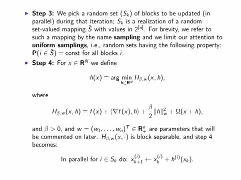
I Step 3: We pick a random set (Sk) of blocks to be updated (inparallel) during that iteration; Sk is a realization of a randomset-valued mapping S with values in 2[n]. For brevity, we refer tosuch a mapping by the name sampling and we limit our attention touniform samplings, i.e., random sets having the following property:P(i ∈ S) = const for all blocks i .

I Step 4: For x ∈ RN we define

h(x) ≡ arg minh∈RN

Hβ,w (x , h),

where

Hβ,w (x , h) ≡ f (x) + 〈∇f (x), h〉+β

2‖h‖2

w + Ω(x + h),

and β > 0, and w = (w1, . . . ,wn)T ∈ Rn+ are parameters that will

be commented on later. Hβ,w (x , ·) is block separable, and step 4becomes:

In parallel for i ∈ Sk do: x(i)k+1 ← x

(i)k + h(i)(xk).

E[F (x + h[S])] = E[f (x + hS) + Ω(x + h[S])]

≤ f (x) +E[|S |]

n

(〈∇f (x), h〉+

β

2‖h‖2

w

)

+

(1− E[|S |]

n

)Ω(x) +

E[|S |]n

Ω(x + h)

=

(1− E[|S |]

n

)F (x) +

E[|S |]n

Hβ,w (x , h)

Hβ,w (x , 0) = F (x)

I Step 5: In some situations we are not able to analyze the iterationcomplexity of PCDM1 (non-strongly-convex F where monotonicityof the method is not guaranteed by other means than by directlyenforcing it by inclusion of Step 5).Let us remark that this issue arises for general Ω only. It does notexist for Ω = 0, Ω(·) = λ‖ · ‖1 and for Ω encoding simple constraintson individual blocks; in these cases one does not need to considerPCDM2.

Contributions

I Problem generality. We give the first complexity analysis for aparallel coordinate descent method in its full generality.

I Partial separability. We give the first analysis of a coordinatedescent type method dealing with a partially separable objective. Inorder to run the method, all we need to know about f are theLipschitz constants Li and the degree of partial separability ω.

I Algorithm unification. Depending on the choice of the blockstructure and the way blocks are selected at every iteration, we givethe first analysis of a method which continuously interpolatesbetween a serial coordinate descent method and the gradientmethod.

I Expected Separable Overapproximation (ESO). En route toproving the iteration complexity results for our algorithms, wedevelop a theory of deterministic and expected separableoverapproximation. We believe this is of independent interest; forinstance, methods based on ESO can be compared favorably to theDiagonal Quadratic Approximation (DQA) approach used in thedecomposition of stochastic optimization programs.

I Variable number of updates per iteration. We give the firstanalysis of a PCDM which allows for a variable number of blocks tobe updated throughout the iterations. This may be useful in somesettings such as when the problem is being solved in parallel by τunreliable processors each of which computes its update h(i)(xk)with probability pb and is busy/down with probability 1− pb.

I Parallelization speedup. We show theoretically and numericallythat PCDM accelerates on its serial counterpart for partiallyseparable problems.

Outline

Introduction


Block Sampling




Block sampling

A sampling S is uniquely characterized by the probability density function

P(S) ≡ P(S = S), S ⊂ [n].

Further we let p = (p1, . . . , pn)T , where

pi ≡ P(i ∈ S).

I A sampling is proper if pi > 0 for all blocks i . PCDM can notconverge for a sampling that is not proper.

I A sampling S is uniform if all blocks get updated with the sameprobability, i.e., if pi = const.

I A sampling S is nil if P(∅) = 1.

Special classes of uniform samplingsI Doubly uniform (DU) samplings: A DU sampling is one which

generates all sets of equal cardinality with equal probability. That isP(S ′) = P(S ′′) whenever |S ′| = |S ′′|. Let qj = P(|S | = j) forj = 0, 1, . . . , n, DU sampling is uniquely characterized by the vectorof probabilities q; its density function is given by

P(S) =q|S|(

n

|S |

) , S ⊆ [n].

I Nonoverlapping uniform (NU) sampling: A NU sampling is onewhich is uniform and which assigns positive probabilities only to setsforming a partition of [n]. Let S1,S2, . . . ,S l be a partition of [n],with ‖S j‖ > 0 for all j . The density function of a NU samplingcorresponding to this partition is given by

P(S) =

1l S ∈ S1,S2, . . . ,S l

0, otherwise

Note that E[|S |] = nl .

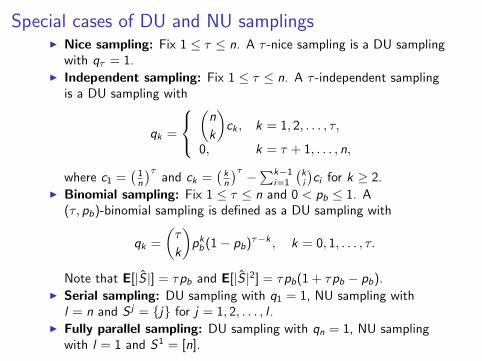
Special cases of DU and NU samplingsI Nice sampling: Fix 1 ≤ τ ≤ n. A τ -nice sampling is a DU sampling

with qτ = 1.I Independent sampling: Fix 1 ≤ τ ≤ n. A τ -independent sampling

is a DU sampling with

qk =

(n

k

)ck , k = 1, 2, . . . , τ,

0, k = τ + 1, . . . , n,

where c1 =(

1n

)τand ck =

(kn

)τ −∑k−1i=1

(ki

)ci for k ≥ 2.

I Binomial sampling: Fix 1 ≤ τ ≤ n and 0 < pb ≤ 1. A(τ, pb)-binomial sampling is defined as a DU sampling with

qk =

(τ

k

)pkb (1− pb)τ−k , k = 0, 1, . . . , τ.

Note that E[|S |] = τpb and E[|S |2] = τpb(1 + τpb − pb).I Serial sampling: DU sampling with q1 = 1, NU sampling with

l = n and S j = j for j = 1, 2, . . . , l .I Fully parallel sampling: DU sampling with qn = 1, NU sampling

with l = 1 and S1 = [n].

Let ∅ 6= J ⊂ [n] and S be any sampling. Further, let g be a blockseparable function, i.e., g(x) =

∑i gi (x (i)), then

E[g(x + hS)] =n∑

i=1

[pigi (x (i) + h(i)) + (1− pi )gi (x (i))].

In addition, if S is a uniform sampling, we have

E[g(x + hS)] =E[|S |]

ng(x + h) +

(1− E[|S |]

n

)g(x).

Outline

Introduction


Block Sampling





DefinitionLet β > 0, w ∈ Rn

+ and let S be a proper uniform sampling. We say that

f : RN → R admits a (β,w)-ESO with respect to S if

E[f (x + h[S])] ≤ f (x) +E[|S |]

n

(〈∇f (x), h〉+

β

2‖h‖2

w

),

holds for all x , h ∈ RN . For simplicity, we write (f , S) ∼ ESO(β,w). Wesay that the ESO is monotonic if F (x + (h(x))[S]) ≤ F (x) with

h(x) = arg minh∈RN Hβ,w (x , h) for all x ∈ domF .

I Inflation. If (f , S) ∼ ESO(β,w), then for β′ ≥ β and w ′ ≥ w ,(f , S) ∼ ESO(β′,w ′).

I Reshuffling. (f , S) ∼ ESO(cβ,w)⇔ (f , S) ∼ ESO(β, cw), c > 0.

I Strong convexity. If (f , S) ∼ ESO(β,w), then β ≥ µf (w).

Deterministic Separable Overapproximation (DSO) ofPartially Separable Functions

TheoremAssume f is partially separable. Letting Supp(h) ≡ i ∈ [n] : h(i) 6= 0,for all h ∈ RN , we have

f (x + h) ≤ f (x) + 〈∇f (x), h〉+maxJ∈J |J ∩ Supp(h)|

2‖h‖2

L.

Outline

Introduction


Block Sampling




Uniform samplings

Consider an arbitrary proper sampling S and let ν = (ν1, . . . , νn)T bedefined by

νi ≡ E[minω, |S ||i ∈ S ] =1

pi

∑

S:i∈S

P(S) minω, |S |, i ∈ [n].

LemmaIf S is proper, then E[f (x + h[S])] ≤ f (x) + 〈∇f (x), h〉p + 1

2‖h‖2pνL.

TheoremIf S is proper and uniform, then

(f , S) ∼ ESO(1, ν L).

If, in addition, P(|S | = τ) = 1 (τ -uniform), then

(f , S) ∼ ESO(minω, τ, L).

Moreover, the ESO is monotonic.

Nonoverlapping uniform samplings

Let S be a (proper) nonoverlapping uniform sampling. If i ∈ S j , for somej ∈ 1, 2, . . . , l, define

γi ≡ maxJ∈J|J ∩ S j |,

and let γ = (γ1, . . . , γn)T .

TheoremIf S is a nonoverlapping uniform sampling, then

(f , S) ∼ ESO(1, γ L).

Moreover, this ESO is monotonic.

Nice samplings

TheoremIf S is the τ -nice sampling and τ 6= 0, then

(f , S) ∼(

1 +(ω − 1)(τ − 1)

max1, n − 1 , L)

Doubly uniform samplings

TheoremIf S is a (proper) doubly uniform sampling, then

(f , S) ∼ ESO

1 +

(ω − 1)(

E[|S|2]

E[|S|] − 1)

max1, n − 1 , L

Summary of results

This theorem could have alternatively been proved by writing S as a convex combination of nicesamplings and applying Theorem 9.

Note that Theorem 15 reduces to that of Theorem 14 in the special case of a nice sampling, andgives the same result as Theorem 13 in the case of the serial and fully parallel samplings.

5.5 Summary of results

In Table 2 we summarize all ESO inequalities established in this section. The first three resultscover all the remaining ones as special cases.

S α β w Monotonic? Follows from

uniform E[|S|]n 1 ν L No Thm 12

nonoverlapping uniform nl 1 γ L Yes Thm 13

doubly uniform E[|S|]n 1 +

(ω−1)

(E[|S|2]

E[|S|] −1

)

max(1,n−1) L No Thm 15

τ -uniform τn minω, τ L Yes Thm 12

τ -nice τn 1 + (ω−1)(τ−1)

max(1,n−1) L No Thm 14/15

(τ, pb)-binomial τpbn 1 + pb(ω−1)(τ−1)

max(1,n−1) L No Thm 15

serial 1n 1 L Yes Thm 13/14/15

fully parallel 1 ω L Yes Thm 13/14/15

Table 2: Values of parameters β and w of an ESO for partially separable f (of degree ω) and variousproper uniform samplings S: (f, S) ∼ ESO(β,w). We also include α = E[|S|]

n as it appears in thecomplexity estimates.

6 Iteration Complexity

In this section we prove two iteration complexity theorems. The first result (Theorem 19) is fornon-strongly-convex F and covers PCDM2 with no restrictions and PCDM1 only in the case whena monotonic ESO is used. The second result (Theorem 20) is for strongly convex F and coversPCDM1 without any monotonicity restrictions. Let us first establish two auxiliary results.

Lemma 16. For all x ∈ domF , Hβ,w(x, h(x)) ≤ miny∈RN F (y) +β−µf (w)

2 ‖y − x‖2w.Proof.

Hβ,w(x, h(x))(17)= min

y∈RNHβ,w(x, y − x) = min

y∈RNf(x) + 〈∇f(x), y − x〉+ Ω(y) + β

2 ‖y − x‖2w(14)≤ min

y∈RNf(y)− µf (w)

2 ‖y − x‖2w + Ω(y) + β2 ‖y − x‖2w.

25

Outline

Introduction


Block Sampling




LemmaFix x0 ∈ RN and let xkk≥0 be a sequence of random vectors in RN withxk+1 depending on xk only. Let φ : RN → R be a nonnegative functionand define ξk = φ(xk). Lastly, choose accuracy level 0 < ε < ξ0,confidence level 0 < ρ < 1, and assume that the sequence of randomvariables ξkk≥0 is nonincreasing and has one of the followingproperties:(i) E[ξk+1|xk ] ≤ (1− ξk

c1)ξk , for all k, where c1 > ε is a contant.

(ii) E[ξk+1|xk ] ≤ (1− 1c2

)ξk , for all k, such that εk ≥ ε, where c2 > 1 is aconstant.if property (i) holds and we choose K ≥ 2 + c1

ε (1− εξ0

+ log( 1ρ )), or if

property (ii) holds, and we choose K ≥ c2 log( ξ0

ερ ), then

P(ξK ≤ ε) ≥ 1− ρ.

Let ξ = F (xk)− F ∗, we have

E[ξk+1|xk ] ≤ (1− α)ξk + α(Hβ,w (xk , h(xk))− F ∗).

We need a upper bound for Hβ,w (xk , h(xk))− F ∗.

Two auxiliary results

From the definition of h(x) and strong convexity of f , we have

LemmaFor all x ∈ dom F , Hβ,w (x , h(x)) ≤ miny∈RNF (y) + β−µf (w)

2 ‖y − x‖2w

Lemma(i) Let x∗ be an optimal solution, x ∈ dom F and let R = ‖x − x∗‖w .Then

Hβ,w (x , h(x))−F ∗ ≤ (

1− F (x)−F∗

2βR2

)(F (x)− F ∗), if F (x)− F ∗ ≤ βR2

12βR2 < 1

2 (F (x)− F ∗), otherwise

(ii) If µf (w) + µΩ(w) > 0 and β ≥ µf (w), then for all x ∈ dom F ,

Hβ,w (x , h(x))− F ∗ ≤ β − µf (w)

β + µΩ(w)(F (x)− F ∗)

Iteration complexity: convex case

TheoremAssume that (f , S) ∼ ESO(β,w), where S is a proper uniform sampling, and

α = E[|S|]n

. Choose x0 ∈ RN satisfying

Rw (x0, x∗) ≡ max

x‖x − x∗‖w : F (x) ≤ F (x0) < +∞,

where x∗ is an optimal point. Further choose target confidence level 0 < ρ < 1,target accuracy level ε > 0 and iteration counter K in any of the following twoways:(i)ε < F (x0)− F ∗ and

K ≥ 2 +2( β

α)max

R2

w (x0, x∗), F (x0)−F∗

β

ε

(1− ε

F (x0)− F ∗+ log

(1

ρ

))(ii)ε < min2( β

α)R2

w (x0, x∗),F (x0)− F ∗ and

K ≥ 2β

αmaxR

2w (x0, x

∗)

ε,1

β log

(F (x0)− F ∗

ερ

)If xk, k ≥ 0 are the random iterates of PCDM2 or PCDM1 if the ESO ismonotonic, then P(F (xK )− F ∗ ≤ ε) ≥ 1− ρ.

Since F (xk) ≤ F (x0) for all k , we have ‖xk − x∗‖w ≤ Rw (x0, x∗).

E[ξk+1|xk ] ≤ (1− α)ξk + α(Hβ,w (xk , h(xk))− F ∗)

≤ (1− α)ξk + αmax

1− ξk

2β‖xk − x∗‖2w

,1

2

ξk

= max

1− αξk

2β‖xk − x∗‖2w

, 1− α

2

ξk

≤ max

1− αξk

2βR2w (x0, x∗)

, 1− α

2

ξk

I Let c1 = 2βα maxR2w (x0, x

∗), ξ0

β , we have E[ξk+1|xk ] ≤ (1− ξkc1

)ξk

I Let c2 = 2βα maxR2w (x0,x

∗)ε , 1

β , we have E[ξk+1|xk ] ≤ (1− 1c2

)ξk .

Speedup factor for convex case

The iteration complexity of our methods in the convex case is O(βα1ε ).

Let us define the parallelization speedup factor by

parallelization speedup factor =βα of the serial methodβα of a parallel method

=n

βα of a parallel method

Speedup for DU samplings

The important message of the above theorem is that the iteration complexity of our methods inthe convex case is O(βα

1ε ). Note that for the serial method (PCDM1 used with S being the serial

sampling) we have α = 1n and β = 1 (see Table 2), and hence β

α = n. It will be interesting to studythe parallelization speedup factor defined by

parallelization speedup factor =βα of the serial methodβα of a parallel method

=n

βα of a parallel method

. (78)

Table 3, computed from the data in Table 2, gives expressions for the parallelization speedupfactors for PCDM based on a DU sampling (expressions for 4 special cases are given as well).

S Parallelization speedup factor

doubly uniform E[|S|]

1+(ω−1)((E[|S|2]/E[|S|])−1)

max(1,n−1)

(τ, pb)-binomial τ1pb

+(ω−1)(τ−1)max(1,n−1)

τ -nice τ

1+(ω−1)(τ−1)max(1,n−1)

fully parallel nω

serial 1

Table 3: Convex F : Parallelization speedup factors for DU samplings. The factors below the lineare special cases of the general expression. Maximum speedup is naturally obtained by the fullyparallel sampling: n

ω .

The speedup of the serial sampling (i.e., of the algorithm based on it) is 1 as we are comparingit to itself. On the other end of the spectrum is the fully parallel sampling with a speedup of n

ω .If the degree of partial separability is small, then this factor will be high — especially so if n ishuge, which is the domain we are interested in. This provides an affirmative answer to the researchquestion stated in italics in the introduction.

Let us now look at the speedup factor in the case of a τ -nice sampling. Letting r = ω−1max(1,n−1) ∈

[0, 1] (degree of partial separability normalized), the speedup factor can be written as

s(r) =τ

1 + r(τ − 1).

Note that as long as r ≤ k−1τ−1 ≈ k

τ , the speedup factor will be at least τk . Also note that max1, τω ≤

s(r) ≤ minτ, nω. Finally, if a speedup of at least s is desired, where s ∈ [0, nω ], one needs to use atleast 1−r

1/s−r processors. For illustration, in Figure 1 we plotted s(r) for a few values of τ . Note thatfor small values of τ , the speedup is significant and can be as large as the number of processors (in

28

Iteration complexity: strongly convex caseF (xk) converges to F ∗ linearly, with high probability.

TheoremAssume F is strongly convex with µf (w) + µΩ(w) > 0. Further, assume(f , S) = ESO(β,w), where S is a proper uniform sampling and let

α = E[|S|]n . Choose initial point x0 ∈ RN , target confidence level

0 < ρ < 1, target accuracy level 0 < ε < F (x0)− F ∗, and

K ≥ 1

α

β + µΩ(w)

µf (w) + µΩ(w)log

(F (x0)− F ∗

ερ

).

If xk are the random points generated by PCDM1 or PCDM2, thenP(F (xK )− F ∗ ≤ ε) ≥ 1− ρ.

E[ξk+1|xk ] ≤ (1− α)ξk + α(Hβ,w (xk , h(xk))− F ∗)

≤(

1− αµf (w) + µΩ(w)

β + µΩ(w)

)ξk ≡ (1− γ)ξk

P[ξK > ε] ≤ E[ξk ]

ε≤ (1− γ)K ξ0

ε≤ ρ

Strongly convex case

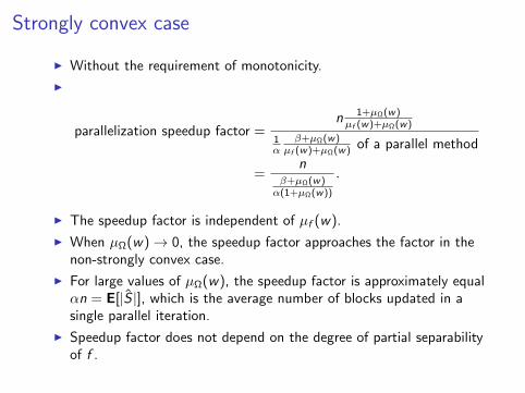
I Without the requirement of monotonicity.

I

parallelization speedup factor =n 1+µΩ(w)µf (w)+µΩ(w)

1α

β+µΩ(w)µf (w)+µΩ(w) of a parallel method

=n

β+µΩ(w)α(1+µΩ(w))

.

I The speedup factor is independent of µf (w).

I When µΩ(w)→ 0, the speedup factor approaches the factor in thenon-strongly convex case.

I For large values of µΩ(w), the speedup factor is approximately equalαn = E[|S |], which is the average number of blocks updated in asingle parallel iteration.

I Speedup factor does not depend on the degree of partial separabilityof f .

Documents

Parallel (Block) Coordinate Descent Methods for Big Data