Embed Size (px)
Citation preview
Distributed Coordinate Descent for Logistic Regression withRegularization
Ilya Tro�mov (Yandex Data Factory)
Alexander Genkin (AVG Consulting)
presented by Ilya Tro�mov
Machine Learning: Prospects and Applications5�8 October 2015, Berlin, Germany
Large Scale Machine Learning
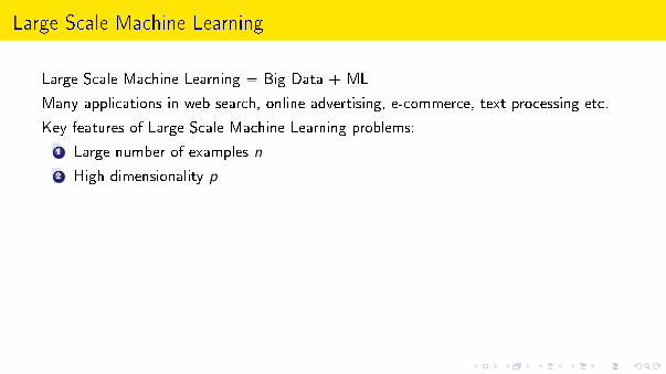
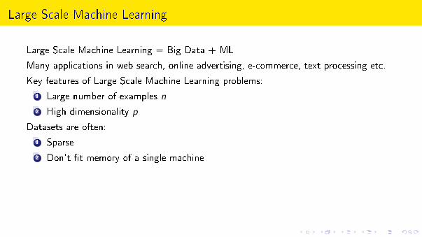
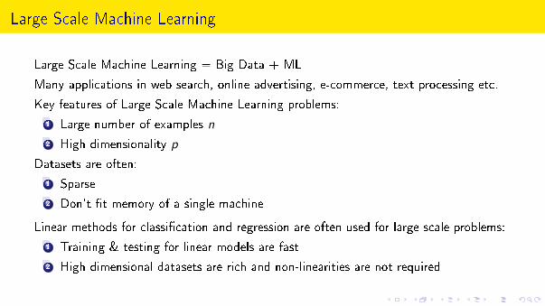
Large Scale Machine Learning = Big Data + ML
Many applications in web search, online advertising, e-commerce, text processing etc.
Key features of Large Scale Machine Learning problems:
1 Large number of examples n
2 High dimensionality p
Datasets are often:
1 Sparse
2 Don't �t memory of a single machine
Linear methods for classi�cation and regression are often used for large-scale problems:
1 Training & testing for linear models are fast
2 High dimensional datasets are rich and non-linearities are not required
Large Scale Machine Learning
Large Scale Machine Learning = Big Data + ML
Many applications in web search, online advertising, e-commerce, text processing etc.
Key features of Large Scale Machine Learning problems:
1 Large number of examples n
2 High dimensionality p
Datasets are often:
1 Sparse
2 Don't �t memory of a single machine
Linear methods for classi�cation and regression are often used for large-scale problems:
1 Training & testing for linear models are fast
2 High dimensional datasets are rich and non-linearities are not required
Binary Classi�cation
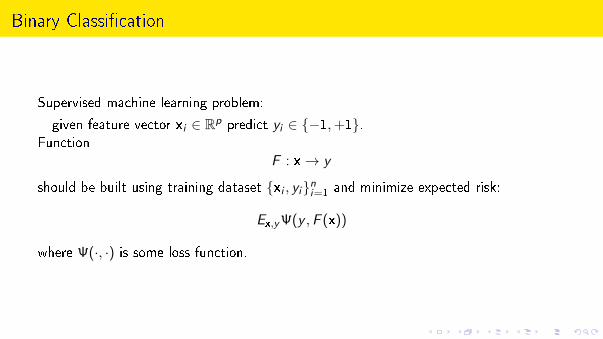
Supervised machine learning problem:
given feature vector xi ∈ Rp predict yi ∈ {−1,+1}.Function
F : x→ y
should be built using training dataset {xi , yi}ni=1and minimize expected risk:
Ex,yΨ(y ,F (x))
where Ψ(·, ·) is some loss function.
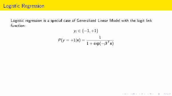
Logistic Regression
Logistic regression is a special case of Generalized Linear Model with the logit link
function:
yi ∈ {−1,+1}
P(y = +1|x) =1
1 + exp(−βTx)
Negated log-likelihood (empirical risk) L(β)
L(β) =n∑
i=1
log(1 + exp(−yiβTxi ))
β∗ = argminβ
L(β)
+ R(β) regularizer
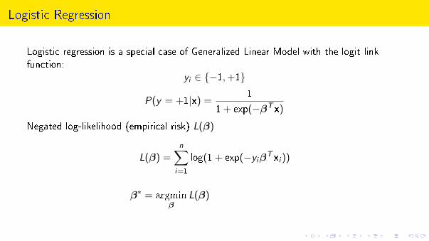
Logistic Regression
Logistic regression is a special case of Generalized Linear Model with the logit link
function:
yi ∈ {−1,+1}
P(y = +1|x) =1
1 + exp(−βTx)
Negated log-likelihood (empirical risk) L(β)
L(β) =n∑
i=1
log(1 + exp(−yiβTxi ))
β∗ = argminβ
L(β)
+ R(β) regularizer
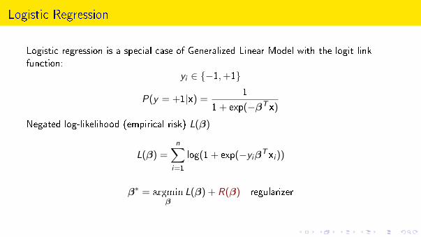
Logistic Regression
Logistic regression is a special case of Generalized Linear Model with the logit link
function:
yi ∈ {−1,+1}
P(y = +1|x) =1
1 + exp(−βTx)
Negated log-likelihood (empirical risk) L(β)
L(β) =n∑
i=1
log(1 + exp(−yiβTxi ))
β∗ = argminβ
L(β) + R(β) regularizer
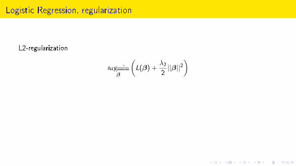
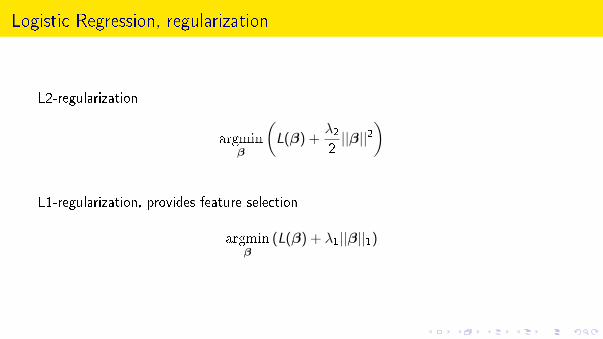
Logistic Regression, regularization
L2-regularization
argminβ
(L(β) +
λ22||β||2
)
L1-regularization, provides feature selection
argminβ
(L(β) + λ1||β||1)
Logistic Regression, regularization
L2-regularization
argminβ
(L(β) +
λ22||β||2
)
L1-regularization, provides feature selection
argminβ
(L(β) + λ1||β||1)
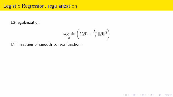
Logistic Regression, regularization
L2-regularization
argminβ
(L(β) +
λ22||β||2
)Minimization of smooth convex function.
Optimization techniques for large datasets
, distributed
SGD
poor parallelization
Conjugate gradients
good parallelization
L-BFGS
good parallelization
Coordinate descent (GLMNET, BBR)
?
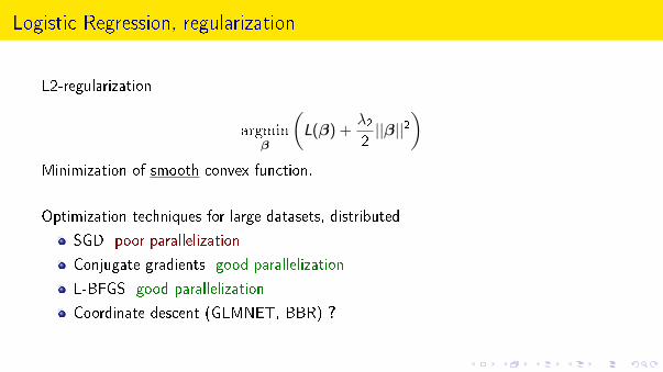
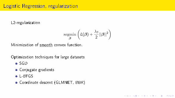
Logistic Regression, regularization
L2-regularization
argminβ
(L(β) +
λ22||β||2
)Minimization of smooth convex function.
Optimization techniques for large datasets, distributed
SGD poor parallelization
Conjugate gradients good parallelization
L-BFGS good parallelization
Coordinate descent (GLMNET, BBR) ?
Logistic Regression, regularization
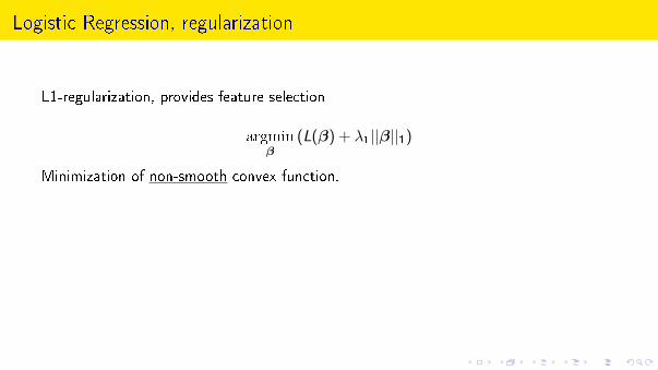
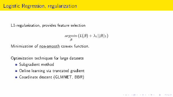
L1-regularization, provides feature selection
argminβ
(L(β) + λ1||β||1)
Minimization of non-smooth convex function.
Optimization techniques for large datasets
, distributed
Subgradient method
slow
Online learning via truncated gradient
poor parallelization
Coordinate descent (GLMNET, BBR)
?
Logistic Regression, regularization
L1-regularization, provides feature selection
argminβ
(L(β) + λ1||β||1)
Minimization of non-smooth convex function.
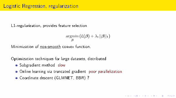
Optimization techniques for large datasets, distributed
Subgradient method slow
Online learning via truncated gradient poor parallelization
Coordinate descent (GLMNET, BBR) ?
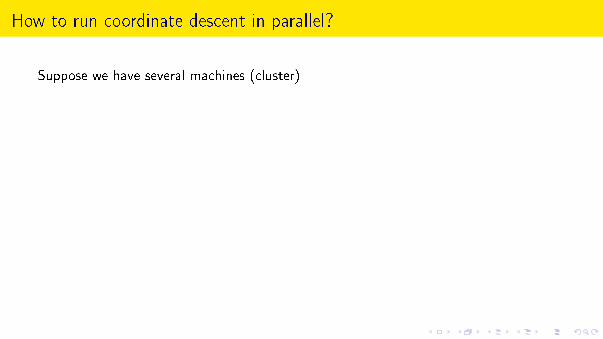
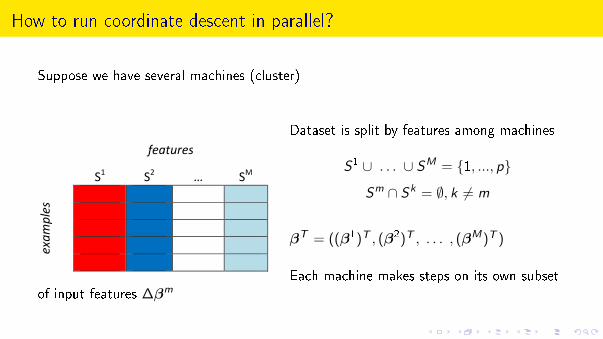
How to run coordinate descent in parallel?
Suppose we have several machines (cluster)
features
S1
S2
… SM
exa
mp
les
Dataset is split by features among machines
S1 ∪ . . . ∪ SM = {1, ..., p}
Sm ∩ Sk = ∅, k 6= m
βT = ((β1)T , (β2)T , . . . , (βM)T )
Each machine makes steps on its own subset
of input features ∆βm
Problems
Two main questions:
1 How to compute ∆βm
2 How to organize communication between machines
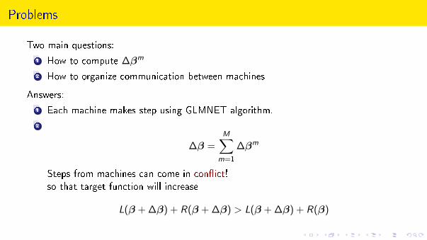
Answers:
1 Each machine makes step using GLMNET algorithm.
2
∆β =M∑
m=1
∆βm
Steps from machines can come in con�ict!
so that target function will increase
L(β + ∆β) + R(β + ∆β) > L(β + ∆β) + R(β)
Problems
Two main questions:
1 How to compute ∆βm
2 How to organize communication between machines
Answers:
1 Each machine makes step using GLMNET algorithm.
2
∆β =M∑
m=1
∆βm
Steps from machines can come in con�ict!
so that target function will increase
L(β + ∆β) + R(β + ∆β) > L(β + ∆β) + R(β)
Problems
Two main questions:
1 How to compute ∆βm
2 How to organize communication between machines
Answers:
1 Each machine makes step using GLMNET algorithm.
2
∆β =M∑
m=1
∆βm
Steps from machines can come in con�ict!
so that target function will increase
L(β + ∆β) + R(β + ∆β) > L(β + ∆β) + R(β)
Problems
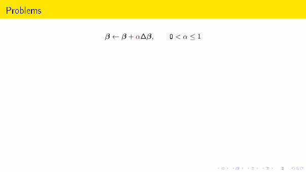
β ← β + α∆β, 0 < α ≤ 1
where α is found by an Armijo rule
L(β + ∆β) + R(β + ∆β) ≤ L(β) + R(β) + ασDk
Dk = ∇L(β)T∆β + R(β + ∆β)− R(β)
L(β + α∆β) =n∑
i=1
log(1 + exp(−yi (β + α∆β)Txi ))
R(β + α∆β) =M∑
m=1
R(βm + α∆βm)
Problems
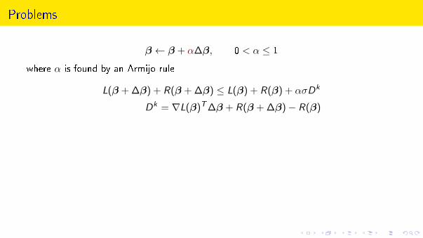
β ← β + α∆β, 0 < α ≤ 1
where α is found by an Armijo rule
L(β + ∆β) + R(β + ∆β) ≤ L(β) + R(β) + ασDk
Dk = ∇L(β)T∆β + R(β + ∆β)− R(β)
L(β + α∆β) =n∑
i=1
log(1 + exp(−yi (β + α∆β)Txi ))
R(β + α∆β) =M∑
m=1
R(βm + α∆βm)
Problems
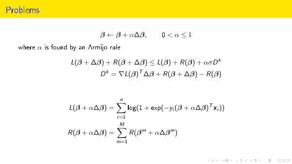
β ← β + α∆β, 0 < α ≤ 1
where α is found by an Armijo rule
L(β + ∆β) + R(β + ∆β) ≤ L(β) + R(β) + ασDk
Dk = ∇L(β)T∆β + R(β + ∆β)− R(β)
L(β + α∆β) =n∑
i=1
log(1 + exp(−yi (β + α∆β)Txi ))
R(β + α∆β) =M∑
m=1
R(βm + α∆βm)
E�ective communication between machines
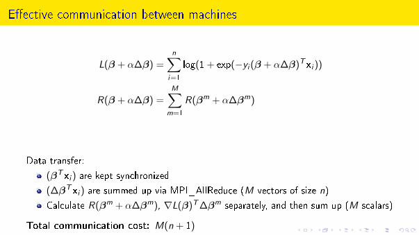
L(β + α∆β) =n∑
i=1
log(1 + exp(−yi (β + α∆β)Txi ))
R(β + α∆β) =M∑
m=1
R(βm + α∆βm)
Data transfer:
(βTxi ) are kept synchronized
(∆βTxi ) are summed up via MPI_AllReduce (M vectors of size n)
Calculate R(βm + α∆βm), ∇L(β)T∆βm separately, and then sum up (M scalars)
Total communication cost: M(n + 1)
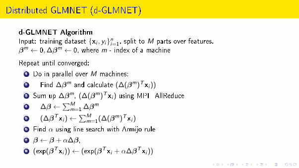
Distributed GLMNET (d-GLMNET)
d-GLMNET AlgorithmInput: training dataset {xi , yi}ni=1
, split to M parts over features.
βm ← 0,∆βm ← 0, where m - index of a machine
Repeat until converged:
1 Do in parallel over M machines:
2 Find ∆βm and calculate (∆(βm)Txi ))
3 Sum up ∆βm, (∆(βm)Txi ) using MPI_AllReduce
4 ∆β ←∑M
m=1∆βm
5 (∆βTxi )←∑M
m=1(∆(βm)Txi )
6 Find α using line search with Armijo rule
7 β ← β + α∆β,
8 (exp(βTxi ))← (exp(βTxi + α∆βTxi ))
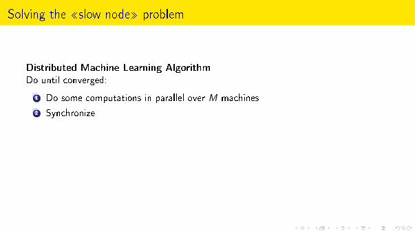
Solving the ¾slow node¿ problem
Distributed Machine Learning AlgorithmDo until converged:
1 Do some computations in parallel over M machines
2 Synchronize
PROBLEM!
M − 1 fast machines will wait for 1 slow
Our solution: machine m at iteration k updates subset Pmk ⊆ Sm of input features at
iteration.
The synchronization is done in separate thread asynchronously, we call it
"Asynchronous Load Balancing" (ALB).
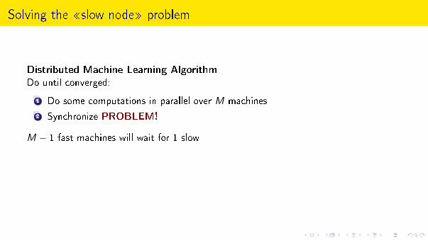
Solving the ¾slow node¿ problem
Distributed Machine Learning AlgorithmDo until converged:
1 Do some computations in parallel over M machines
2 Synchronize PROBLEM!
M − 1 fast machines will wait for 1 slow
Our solution: machine m at iteration k updates subset Pmk ⊆ Sm of input features at
iteration.
The synchronization is done in separate thread asynchronously, we call it
"Asynchronous Load Balancing" (ALB).
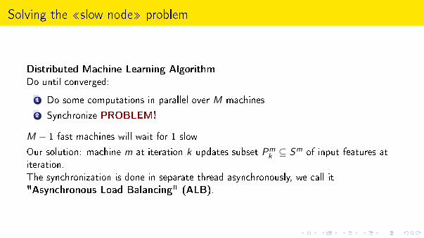
Solving the ¾slow node¿ problem
Distributed Machine Learning AlgorithmDo until converged:
1 Do some computations in parallel over M machines
2 Synchronize PROBLEM!
M − 1 fast machines will wait for 1 slow
Our solution: machine m at iteration k updates subset Pmk ⊆ Sm of input features at
iteration.
The synchronization is done in separate thread asynchronously, we call it
"Asynchronous Load Balancing" (ALB).
Theoretical Results
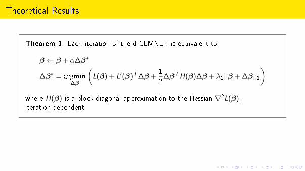
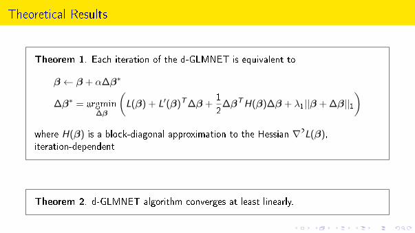
Theorem 1. Each iteration of the d-GLMNET is equivalent to
β ← β + α∆β∗
∆β∗ = argmin∆β
(L(β) + L′(β)T∆β +
1
2∆βTH(β)∆β + λ1||β + ∆β||1
)where H(β) is a block-diagonal approximation to the Hessian ∇2L(β),iteration-dependent
Theorem 2. d-GLMNET algorithm converges at least linearly.
Theoretical Results
Theorem 1. Each iteration of the d-GLMNET is equivalent to
β ← β + α∆β∗
∆β∗ = argmin∆β
(L(β) + L′(β)T∆β +
1
2∆βTH(β)∆β + λ1||β + ∆β||1
)where H(β) is a block-diagonal approximation to the Hessian ∇2L(β),iteration-dependent
Theorem 2. d-GLMNET algorithm converges at least linearly.
Numerical Experiments
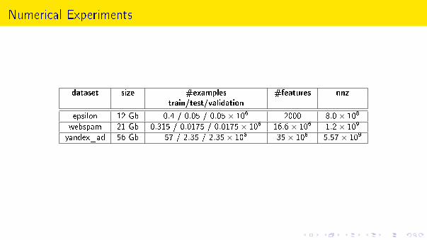
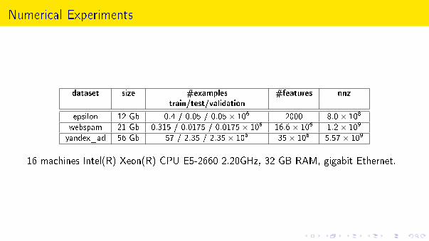
dataset size #examples #features nnztrain/test/validation
epsilon 12 Gb 0.4 / 0.05 / 0.05× 10⁶ 2000 8.0× 10⁸
webspam 21 Gb 0.315 / 0.0175 / 0.0175× 10⁶ 16.6× 10⁶ 1.2× 10⁹
yandex_ad 56 Gb 57 / 2.35 / 2.35× 10⁶ 35× 106 5.57× 10⁹
16 machines Intel(R) Xeon(R) CPU E5-2660 2.20GHz, 32 GB RAM, gigabit Ethernet.
Numerical Experiments
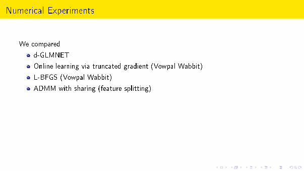
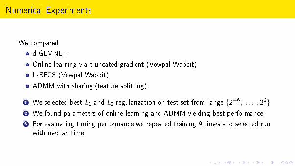
We compared
d-GLMNET
Online learning via truncated gradient (Vowpal Wabbit)
L-BFGS (Vowpal Wabbit)
ADMM with sharing (feature splitting)
1 We selected best L1 and L2 regularization on test set from range {2−6, . . . , 26}2 We found parameters of online learning and ADMM yielding best performance
3 For evaluating timing performance we repeated training 9 times and selected run
with median time
Numerical Experiments
We compared
d-GLMNET
Online learning via truncated gradient (Vowpal Wabbit)
L-BFGS (Vowpal Wabbit)
ADMM with sharing (feature splitting)
1 We selected best L1 and L2 regularization on test set from range {2−6, . . . , 26}2 We found parameters of online learning and ADMM yielding best performance
3 For evaluating timing performance we repeated training 9 times and selected run
with median time
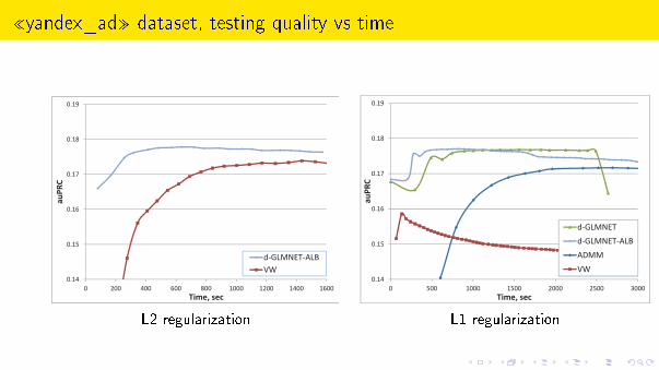
¾yandex_ad¿ dataset, testing quality vs time
����
����
����
����
����
���
� �� ��� ��� ��� ���� ��� ���� ����
�����
�����
�� ���������
��
����
����
����
����
����
���
� ��� ���� ���� ��� ��� ����
�����
�����
� ������
� ������ ���
����
��
L2 regularization L1 regularization
Conclusions & Future Work
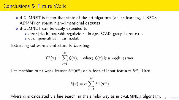
d-GLMNET is faster that state-of-the-art algoritms (online learning, L-BFGS,
ADMM) on sparse high-dimensional datasets
d-GLMNET can be easily extended toother [block-]separable regularizers: bridge, SCAD, group Lasso, e.t.c.other generalized linear models
Extending software architecture to boosting
F ∗(x) =M∑i=1
fi (x), where fi (x) is a week learner
Let machine m �t weak learner f mi (xm) on subset of input features Sm. Then
fi (x) = αM∑
m=1
f mi (xm)
where α is calculated via line search, in the similar way as in d-GLMNET algorithm.
Conclusions & Future Work
d-GLMNET is faster that state-of-the-art algoritms (online learning, L-BFGS,
ADMM) on sparse high-dimensional datasets
d-GLMNET can be easily extended toother [block-]separable regularizers: bridge, SCAD, group Lasso, e.t.c.other generalized linear models
Extending software architecture to boosting
F ∗(x) =M∑i=1
fi (x), where fi (x) is a week learner
Let machine m �t weak learner f mi (xm) on subset of input features Sm. Then
fi (x) = α
M∑m=1
f mi (xm)
where α is calculated via line search, in the similar way as in d-GLMNET algorithm.
Conclusions & Future Work
Software implementation:
https://github.com/IlyaTrofimov/dlr
paper is available by request :
Ilya Tro�mov - [email protected]
Conclusions & Future Work
Software implementation:
https://github.com/IlyaTrofimov/dlr
paper is available by request :
Ilya Tro�mov - [email protected]

Thank you :)Questions ?


![arXiv:1711.10467v3 [cs.LG] 30 Jul 2019Implicit Regularization in Nonconvex Statistical Estimation: Gradient Descent Converges Linearly for Phase Retrieval, Matrix Completion, and Blind](https://img.dokumen.tips/doc/110x75/5f05e0327e708231d41527c4/arxiv171110467v3-cslg-30-jul-2019-implicit-regularization-in-nonconvex-statistical.jpg)