ASYNCHRONOUS STOCHASTIC COORDINATE DESCENT:PARALLELISM AND CONVERGENCE PROPERTIES

JI LIU∗ AND STEPHEN J. WRIGHT†

Abstract. We describe an asynchronous parallel stochastic proximal coordinate descent algo-rithm for minimizing a composite objective function, which consists of a smooth convex functionplus a separable convex function. In contrast to previous analyses, our model of asynchronous com-putation accounts for the fact that components of the unknown vector may be written by some coressimultaneously with being read by others. Despite the complications arising from this possibility,the method achieves a linear convergence rate on functions that satisfy an optimal strong convexityproperty and a sublinear rate (1/k) on general convex functions. Near-linear speedup on a mul-ticore system can be expected if the number of processors is O(n1/4). We describe results fromimplementation on ten cores of a multicore processor.

Key words. stochastic coordinate descent, asynchronous parallelism, inconsistent read, com-posite objective

AMS subject classifications. 90C25, 68W20, 68W10, 90C05

1. Introduction. We consider the convex optimization problem

minx

F (x) := f(x) + g(x), (1.1)

where f : Rn 7→ R is a smooth convex function and g : Rn 7→ R∪ ∞ is a separable,closed, convex, and extended real-valued function. “Separable” means that g(x) canbe expressed as g(x) =

∑ni=1 gi((x)i), where (x)i denotes the ith element of x and

each gi : R 7→ R ∪ ∞, i = 1, 2, . . . , n is a closed, convex, and extended real-valuedfunction.

Formulations of the type (1.1) arise in many data analysis and machine learningproblems, for example, the linear primal or nonlinear dual formulation of supportvector machines [9], the LASSO approach to regularized least squares, and regular-ized logistic regression. Algorithms based on gradient and approximate / partialgradient information have proved effective in these settings. We mention in partic-ular gradient projection and its accelerated variants [28], proximal gradient [42] andaccelerated proximal gradient [4] methods for regularized objectives, and stochasticgradient methods [27, 36]. These methods are inherently serial, in that each iter-ation depends on the result of the previous iteration. Recently, parallel multicoreversions of stochastic gradient and stochastic coordinate descent have been describedfor problems involving large data sets; see for example [30, 33, 3, 20, 37, 21].

This paper proposes an asynchronous stochastic proximal coordinate-descent al-gorithm, called AsySPCD, for composite objective functions. The basic step ofAsySPCD, executed repeatedly by each core of a multicore system, is as follows:Choose an index i ∈ 1, 2, . . . , n; read x from shared memory and evaluate theith element of ∇f ; subtract a short, constant, positive of this partial gradient from(x)i; and perform a proximal operation on (x)i to account for the regularization termgi(·). We use a simple model of computation that matches well to modern multi-core architectures. Each core performs its updates on centrally stored vector x in an

∗Department of Computer Sciences, University of Wisconsin-Madison, 1210 W. Dayton St., Madi-son, WI 53706-1685, US (ji-liu@cs.wisc.edu)†Department of Computer Sciences, University of Wisconsin-Madison, 1210 W. Dayton St., Madi-

son, WI 53706-1685, US (swright@cs.wisc.edu)

1

2

asynchronous, uncoordinated fashion, without any form of locking. A consequenceof this model is that the version of x that is read by a core in order to evalute itsgradient is usually not the same as the version to which the update is made later, asit is updated in the interim by other cores. (Generally, we denote by x the version ofx that is used by a core to evalaute its component of ∇f(x).) We assume, however,that indefinite delays do not occur between reading and updating: There is a bound τsuch no more than τ component-wise updates to x are missed by a core, between thetime at which it reads the vector x and the time at which it makes its update to thechosen element of x. A similar model of parallel asynchronous computation was usedin Hogwild! [30] and AsySCD [20]. However, there is a key difference in this paper:We do not assume that the evaluation vector x is a version of x that actually existedin the shared memory at some point in time. Rather, we account for the fact that thecomponents of x may be updated by multiple cores while in the process of being readby another core, so that x may be a “hybrid” version that never actually existed inmemory. Our new model, which we call an “inconsistent read” model, is significantlycloser to the reality of asynchronous computation, and dispenses with the somewhatunsatisfying “consistent read” assumption of previous work. It also requires a quitedistinct style of analysis; our proofs differ substantially from those in previous relatedworks.

We show that, for suitable choices of steplength, our algorithm converges at alinear rate if an “optimal strong convexity” property (1.2) holds. It attains sublinearconvergence at a “1/k” rate for general convex functions. Our analysis also defines asufficient condition for near-linear speedup in the number of cores used. This condi-tion relates the value of delay parameter τ (which corresponds closely to the numberof cores / threads used in the computation) to the problem dimension n. A parameterthat quantifies the cross-coordinate interactions in ∇f also appears in this relation-ship. When the Hessian of f is nearly diagonal, the minimization problem is almostseparable, so higher degrees of parallelism are possible.

We review related work in Section 2. Section 3 specifies the proposed algorithm.Convergence results are described in Section 4, with proofs given in the appendix.Computational experience is reported in Section 5. A summary and conclusions ap-pear in Section 6.

Notation and Assumption. We use the following notation in the remainder ofthe paper.

• Ω denotes the intersection of dom(f) and dom(g)• S denotes the set on which F attains its optimal value, which is denoted byF ∗.

• PS(·) denotes Euclidean-norm projection onto S.• ei denotes the ith natural basis vector in Rn.• Given a matrix A, we use A·j to denote its jth column and Ai· to denote itsith row.

• ‖ · ‖ denotes the Euclidean norm ‖ · ‖2.• xj ∈ Rn denotes the jth iterate generated by the algorithm.• f∗j := f(PS(xj)) and g∗j := f(PS(xj)).• F ∗ := F (PS(x)) denotes the optimal objective value. (Note that F ∗ = f∗j +g∗j

for any j.)• We use (x)i for the ith element of x, and ∇if(x), (∇f(x))i, or ∂f/∂xi for

the ith element of ∇f(x).

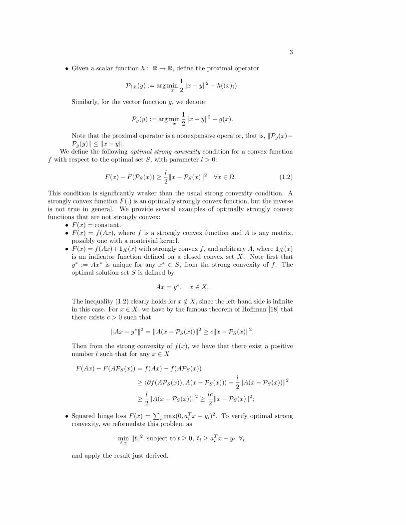
3

• Given a scalar function h : R→ R, define the proximal operator

Pi,h(y) := arg minx

1

2‖x− y‖2 + h((x)i).

Similarly, for the vector function g, we denote

Pg(y) := arg minx

1

2‖x− y‖2 + g(x).

Note that the proximal operator is a nonexpansive operator, that is, ‖Pg(x)−Pg(y)‖ ≤ ‖x− y‖.

We define the following optimal strong convexity condition for a convex functionf with respect to the optimal set S, with parameter l > 0:

F (x)− F (PS(x)) ≥ l

2‖x− PS(x)‖2 ∀x ∈ Ω. (1.2)

This condition is significantly weaker than the usual strong convexity condition. Astrongly convex function F (.) is an optimally strongly convex function, but the inverseis not true in general. We provide several examples of optimally strongly convexfunctions that are not strongly convex:

• F (x) = constant.• F (x) = f(Ax), where f is a strongly convex function and A is any matrix,

possibly one with a nontrivial kernel.• F (x) = f(Ax)+1X(x) with strongly convex f , and arbitrary A, where 1X(x)

is an indicator function defined on a closed convex set X. Note first thaty∗ := Ax∗ is unique for any x∗ ∈ S, from the strong convexity of f . Theoptimal solution set S is defined by

Ax = y∗, x ∈ X.

The inequality (1.2) clearly holds for x /∈ X, since the left-hand side is infinitein this case. For x ∈ X, we have by the famous theorem of Hoffman [18] thatthere exists c > 0 such that

‖Ax− y∗‖2 = ‖A(x− PS(x))‖2 ≥ c‖x− PS(x)‖2.

Then from the strong convexity of f(x), we have that there exist a positivenumber l such that for any x ∈ X

F (Ax)− F (APS(x)) = f(Ax)− f(APS(x))

≥ 〈∂f(APS(x)), A(x− PS(x))〉+l

2‖A(x− PS(x))‖2

≥ l

2‖A(x− PS(x))‖2 ≥ lc

2‖x− PS(x)‖2;

• Squared hinge loss F (x) =∑i max(0, aTi x − yi)2. To verify optimal strong

convexity, we reformulate this problem as

mint,x‖t‖2 subject to t ≥ 0, ti ≥ aTi x− yi ∀i,

and apply the result just derived.

4

Note that optimal strong convexity (1.2) is a weaker version of the “essentialstrong convexity” condition used in [20]. A concept called “restricted strong convex-ity” proposed in [19] (See Lemma 4.6) is similar in that it requires a certain quantityto increase quadratically with distance from the solution set, but different in that theobjective is assumed to be differentiable. Anitescu [2] defines a “quadratic growthcondition” for (smooth) nonlinear programming in which the objective is assumed togrow at least quadratically with distance to a local solution in some feasible neighbor-hood of that solution. Since our setting (unconstrained, nonsmooth, convex) is quitedifferent, we believe the use of a different term is warranted here.

Throughout this paper, we make the following assumption.Assumption 1. The optimal solution set S of (1.1) is nonempty.

Lipschitz Constants. We define two different Lipschitz constants Lres and Lmax

that are critical to the analysis, as follows. Lres is the restricted Lipschitz constant for∇f along the coordinate directions: For any x ∈ Ω, for any i = 1, 2, . . . , n, and anyt ∈ R such that x+ tei ∈ Ω, we have

‖∇f(x)−∇f(x+ tei)‖ ≤ Lres|t|.

The coordinate Lipschitz constant Lmax is defined for x, i, t satisfying the same con-ditions as above:

‖∇f(x)−∇f(x+ tei)‖∞ ≤ Lmax|t|.

Note that

f(x+ tei)− f(x) ≤ 〈∇if(x), t〉+Lmax

2t2. (1.3)

We denote the ratio between these two quantities by Λ:

Λ := Lres/Lmax. (1.4)

Making the implicit assumption that Lres and Lmax are chosen to be the smallestvalues that satisfy their respective definitions, we have from standard relationshipsbetween the `2 and `∞ norms that

1 ≤ Λ ≤√n.

Besides bounding the nonlinearity of f along various directions, the quantities Lres

and Lmax capture the interactions between the various components in the gradient∇f . In the case of twice continuously differentiable f , we can understand theseinteractions by observing the diagonal and off-diagonal terms of the Hessian ∇2f(x).

Let us consider upper bounds on the ratio Λ in various situations. For simplicity,we suppose that f is quadratic with positive semidefinite Hessian Q.

• If Q is sparse with at most p nonzeros per row/column, we have that

Lres = maxi‖Q·i‖2 ≤

√pmax

i‖Q·i‖∞ =

√pLmax,

so that Λ ≤ √p in this situation.• If Q is diagonally dominant, we have for any column i that

‖Q·i‖2 ≤ Qii + ‖[Qji]j 6=i‖2 ≤ Qii +∑j 6=i

|Qji| ≤ 2Qii,

which, by taking the maximum of both sides, implies that Λ ≤ 2 in this case.

5

• Suppose that Q = ATA, where A ∈ Rm×n is a random matrix whose entriesare i.i.d from N (0, 1). (For example, we could be solving the linear least-squares problem f(x) = 1

2‖Ax − b‖2). We show in [20] that Λ is upper-

bounded roughly by 1 +√n/m in this case.

2. Related Work. We have surveyed related work on coordinate descent andstochastic gradient methods in a recent report [20]. Our discussion there includednon-stochastic, cyclic coordinate descent methods [38, 23, 41, 5, 39, 40], synchronousparallel methods that distribute the work of function and gradient evaluation [15, 24,17, 7, 11, 1, 10, 35], and asynchronous parallel stochastic gradient methods (includingthe randomized Kaczmarz algorithm) [30, 21]. We make some additional commentshere on related topics, and include some recent references from this active researcharea.

Stochastic coordinate descent can be viewed as a special case of stochastic gradient,so analysis of the latter approach can be applied, to obtain for example a sublinear 1/krate of convergence in expectation for strongly convex functions; see, for example [27].However, stochastic coordinate descent is “special” in that it is possible to guaranteeimprovement in the objective at every step. Nesterov [29] studied the convergencerate for a stochastic block coordinate descent method for unconstrained and separablyconstrained convex smooth optimization, proving linear convergence for the stronglyconvex case and a sublinear 1/k rate for the convex case. Richtarik and Takac [32] andLu and Xiao [22] extended this work to composite minimization, in which the objectiveis the sum of a smooth convex function and a separable nonsmooth convex function,and obtained similar (slightly stronger) convergence results. Stochastic coordinatedescent is extended by Necoara and Patrascu [26] to convex optimization with asingle linear constraint, randomly updating two coordinates at a time to maintainfeasibility.

In the class of synchronous parallel methods for coordinate descent, Richtarik andTakac [33] studied a synchronized parallel block (or minibatch) coordinate descent al-gorithm for composite optimization problems of the form (1.1), with a block separableregularizer g. At each iteration, processors update the randomly selected coordinatesconcurrently and synchronously. Speedup depends on the sparsity of the data matrixthat defines the loss functions. A similar synchronous parallel method was studied in[25] and [8]; the latter focuses on the case of g(x) = ‖x‖1. Scherrer et al. [34] makegreedy choices of multiple blocks of variables to update in parallel. Another greedyway of selecting coordinates was considered by Peng et al. [31], who also describe aparallel implementation of FISTA, an accelerated first-order algorithm due to Beckand Teboulle [4]. Fercoq and Richtarik [14] consider a variant of (1.1) in which fis allowed to be nonsmooth. They apply Nesterov’s smoothing scheme to obtain asmoothed version and update multiple blocks of coordinates using block coordinatedescent in parallel. Sublinear convergence rate is established for both strongly convexand weakly convex cases. Fercoq and Richtarik [13] applies Nesterov’s acceleratedscheme to the synchronous parallel block coordinate algorithm of [33], and providesan improved sublinear convergence rate, whose efficiency again depends on sparsityin the data matrix.

We turn now to asynchronous parallel methods. Bertsekas and Tsitsiklis [6] de-scribed an asynchronous method for fixed-point problems x = q(x) over a separableconvex closed feasible region. (The optimization problem (1.1) can be formulated inthis way by defining q(x) := Pαg[(I − α∇f)(x)] for a fixed α > 0.) They use aninconsistent-read model of asynchronous computation, and establish linear conver-

6

gence provided that components are not neglected indefinitely and that the iterationx = q(x) is a maximum-norm contraction. The latter condition is quite strong. Inthe case of g null and f convex quadratic in (1.1) for instance, it requires the Hes-sian to satisfy a diagonal dominance condition — a stronger condition than strongconvexity. By comparison, AsySCD [20] guarantees linear convergence under an“essential strong convexity” condition, though it assumes a consistent-read model ofasynchronous computation. Elsner et al. [12] considered the same fixed point problemand architecture as [6], and describe a similar scheme. Their scheme appears to re-quire locking of the shared-memory data structure for x to ensure consistent readingand writing. Frommer and Szyld [16] give a comprehensive survey of asynchronousmethods for solving fixed-point problems.

Liu et al. [20] followed the asynchronous consistent-read model of Hogwild! todevelop an asynchronous stochastic coordinate descent (AsySCD) algorithm andproved sublinear (1/k) convergence on general convex functions and a linear conver-gence rate on functions that satisfy an “essential strong convexity” property. Sridharet al. [37] developed an efficient LP solver by relaxing an LP problem into a bound-constrained QP problem, which is then solved by AsySCD.

Liu et al. [21] developed an asynchronous parallel variant of the randomizedKaczmarz algorithm for solving a general consistent linear system Ax = b, prov-ing a linear convergence rate. Avron et al. [3] proposed an asynchronous solverfor the system Qx = c where Q is a symmetric positive definite matrix, proving alinear convergence rate. This method is essentially an asynchronous stochastic coor-dinate descent method applied to the strongly convex quadratic optimization problemminx

12x

TQx−cTx. The paper considers both inconsistent- and consistent-read casesare considered, with slightly different convergence results.

3. Algorithm. In our algorithm AsySPCD, multiple processors have access toa shared data structure for the vector x, and each processor is able to compute arandomly chosen element of the gradient vector ∇f(x). Each processor repeatedlyruns the following proximal coordinate descent process. (Choice of the steplengthparameter γ is discussed further in the next section.)

R: Choose an index i ∈ 1, 2, . . . , n at random, read x into the local storagelocation x, and evaluate ∇if(x);

U: Update component i of the shared x by taking a step of length γ/Lmax in thedirection −∇if(x), follows by a proximal operation:

x← Pi, γLmax

gi

(x− γ

Lmaxei∇if(x)

).

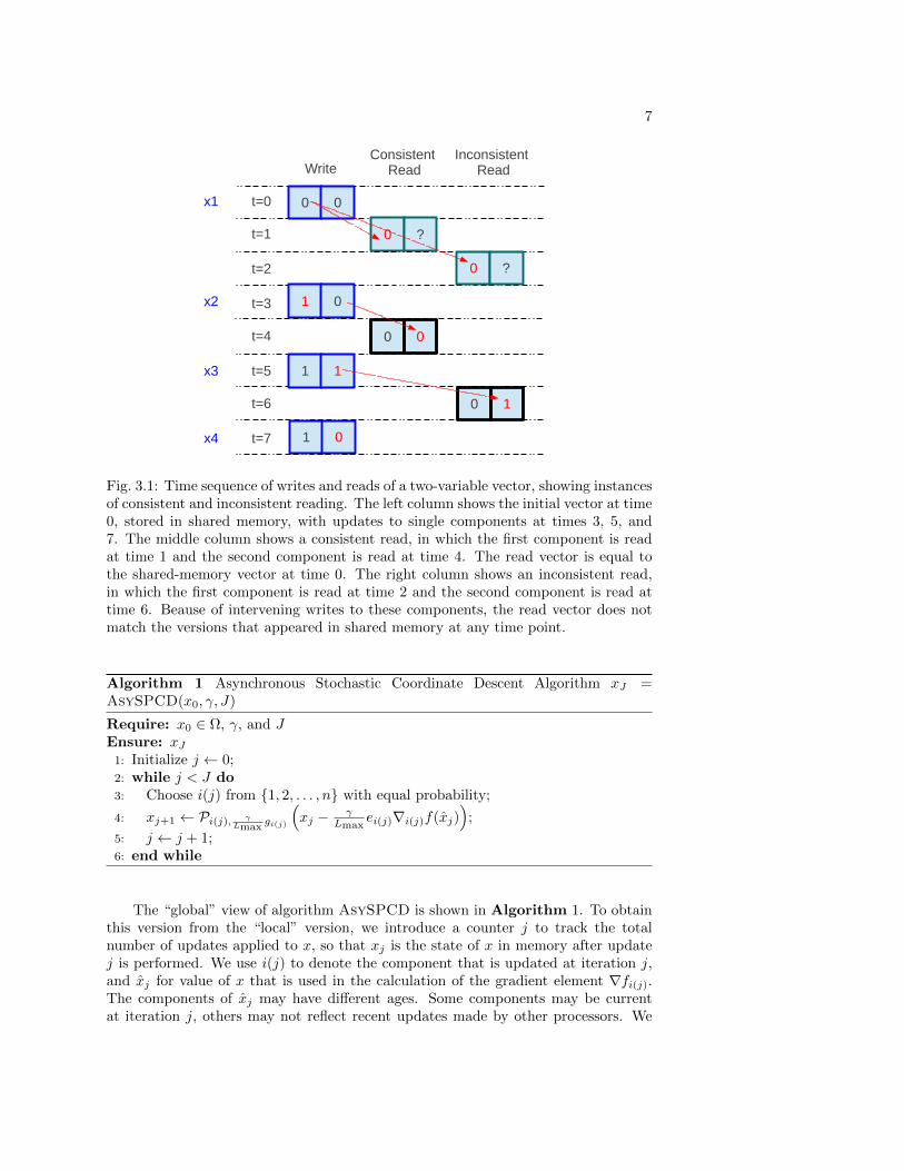
Notice that each step changes just a single element of x, that is, the ith element. Unlikestandard proximal coordinate descent, the value x at which the coordinate gradient iscalculated usually differs from the value of x to which the update is applied, becausewhile the processor is evaluating its gradient, other processors may repeatedly updatethe value of x stored in memory. As mentioned above, we used an “inconsistent read”model of asynchronous computation here, in contrast to the “consistent read” modelsof AsySCD [20] and Hogwild! [30]. Figure 3.1 shows how inconsistent reading canoccur, as a result of updating of components of x while it is being read. Consistentreading can be guaranteed only by means of a software lock, but such a mechanismdegrades parallel performance significantly. In fact, the implementations of Hogwild!and AsySCD described in the papers [30, 20] do not use any software lock, and in thisrespect the computations in those papers are not quite compatible with the analysis.

7

Fig. 3.1: Time sequence of writes and reads of a two-variable vector, showing instancesof consistent and inconsistent reading. The left column shows the initial vector at time0, stored in shared memory, with updates to single components at times 3, 5, and7. The middle column shows a consistent read, in which the first component is readat time 1 and the second component is read at time 4. The read vector is equal tothe shared-memory vector at time 0. The right column shows an inconsistent read,in which the first component is read at time 2 and the second component is read attime 6. Beause of intervening writes to these components, the read vector does notmatch the versions that appeared in shared memory at any time point.

Algorithm 1 Asynchronous Stochastic Coordinate Descent Algorithm xJ =AsySPCD(x0, γ, J)

Require: x0 ∈ Ω, γ, and JEnsure: xJ1: Initialize j ← 0;2: while j < J do3: Choose i(j) from 1, 2, . . . , n with equal probability;

4: xj+1 ← Pi(j), γLmax

gi(j)

(xj − γ

Lmaxei(j)∇i(j)f(xj)

);

5: j ← j + 1;6: end while

The “global” view of algorithm AsySPCD is shown in Algorithm 1. To obtainthis version from the “local” version, we introduce a counter j to track the totalnumber of updates applied to x, so that xj is the state of x in memory after updatej is performed. We use i(j) to denote the component that is updated at iteration j,and xj for value of x that is used in the calculation of the gradient element ∇fi(j).The components of xj may have different ages. Some components may be currentat iteration j, others may not reflect recent updates made by other processors. We

8

assume however that there is an upper bound of τ on the age of each component,measured in terms of updates. K(j) defines an iterate set such that

xj = xj +∑

d∈K(j)

(xd+1 − xd).

One can see that d ≤ j − 1 ∀d ∈ K(j). Here we assume τ to be the upper boundon the age of all elements in K(j), for all j, so that τ ≥ j −mind | d ∈ K(j). Weassume further that K(j) is ordered from oldest to newest index (that is, smallestto largest). Note that K(j) is empty if xj = xj , that is, if the step is simply anordinary stochastic coordinate gradient update. The value of τ corresponds closely tothe number of processors involved in the computation.

4. Main Results. This section presents results on convergence of AsySPCD.The theorem encompasses both the linear rate for optimally strongly convex f andthe sublinear rate for general convex f . The result depends strongly on the delayparameter τ . The proofs are highly technical, and are relegated to Appendix A. Wenote the proof techniques differ significantly from those used for the consistent-readalgorithms of [30] and [20].

We start by describing the key idea of the algorithm, which is reflected in the waythat it chooses the steplength parameter γ. Denoting xj+1 by

xj+1 := P γLmax

g

(xj −

γ

Lmax∇f(xj)

), (4.1)

we can see that

(xj+1)i(j) = (xj+1)i(j), (xj+1)i = (xj)i for i 6= i(j),

so that xj+1 − xj = [(xj+1)i(j) − (xj)i(j)]ei(j). Thus, we have

Ei(j)(xj+1 − xj) =1

n

n∑i=1

[(xj+1)i − (xj)i]ei =1

n[xj+1 − xj ].

Therefore, we can view xj+1−xj as capturing the expected behavior of xj+1−xj . Notethat when g(x) = 0, we have xj+1 − xj = −(γ/Lmax)∇f(xj), a standard negative-gradient step. The choice of steplength parameter γ entails a tradeoff: We would likeγ to be long enough that significant progress is made at each step, but not so longthat the gradient information computed at xj is stale and irrelevant by the time theupdate is applied to xj . We enforce this tradeoff by means of a bound on the ratio ofexpected squared norms on xj − xj+1 at successive iterates; specifically,

E‖xj−1 − xj‖2 ≤ ρE‖xj − xj+1‖2, (4.2)

where ρ > 1 is a user defined parameter. The analysis becomes a delicate balancingact in the choice of ρ and steplength γ between aggression and excessive conservatism.We find, however, that these values can be chosen to ensure steady convergence for theasynchronous method at a linear rate, with rate constants that are almost consistentwith a standard short-step proximal full-gradient descent, when the optimal strongconvexity condition (1.2) is satisfied.

Our main convergence result is the following.

9

Theorem 4.1. Suppose that Assumption 1 is satisfied. Let ρ be a constant thatsatisfies ρ > 1 + 4/

√n, and define the quantities θ, θ′, and ψ as follows:

θ :=ρ(τ+1)/2 − ρ1/2

ρ1/2 − 1, θ′ :=

ρ(τ+1) − ρρ− 1

, ψ := 1 +τθ′

n+

Λθ√n. (4.3)

Suppose that the steplength parameter γ > 0 satisfies the following two bounds:

γ ≤ 1

ψ, γ ≤

√n(1− ρ−1)− 4

4(1 + θ)Λ. (4.4)

Then we have

E‖xj−1 − xj‖2 ≤ ρE‖xj − xj+1‖2, j = 1, 2, . . . . (4.5)

If the optimal strong convexity property (1.2) holds with l > 0, we have for j = 1, 2, . . .that

E‖xj − PS(xj)‖2 +2γ

Lmax(EF (xj)− F ∗)

≤(

1− l

n(l + γ−1Lmax)

)j (‖x0 − PS(x0)‖2 +

2γ

Lmax(F (x0)− F ∗)

), (4.6)

while for general smooth convex function f , we have

EF (xj)− F ∗ ≤n(‖x0 − PS(x0)‖2Lmax + 2γ(F (x0)− F ∗))

2γ(n+ j). (4.7)

The following corollary proposes an interesting particular choice for the parame-ters for which the convergence expressions become more comprehensible. The resultrequires a condition on the delay bound τ in terms of n and the ratio Λ.

Corollary 4.2. Suppose that Assumption 1 holds and that

4eΛ(τ + 1)2 ≤√n. (4.8)

If we choose

ρ =

(1 +

4eΛ(τ + 1)√n

)2

, (4.9)

then the steplength γ = 1/2 will satisfy the bounds (4.4). In addition, when theoptimal strong convexity property (1.2) holds with l > 0, we have for j = 1, 2, . . . that

EF (xj)− F ∗ ≤(

1− l

n(l + 2Lmax)

)j(Lmax‖x0 − PS(x0)‖2 + F (x0)− F ∗), (4.10)

while for the case of general convex f , we have

EF (xj)− F ∗ ≤n(Lmax‖x0 − PS(x0)‖2 + F (x0)− F ∗)

j + n. (4.11)

We note that the linear rate (4.10) is broadly consistent with the linear rate forthe classical steepest descent method applied to strongly convex functions, which has

10

a rate constant of (1 − 2l/L), where L is the standard Lipschitz constant for ∇f .Suppose we assume (not unreasonably) that n steps of stochastic coordinate descentcost roughly the same as one step of steepest descent, and that l ≤ Lmax. It followsfrom (4.10) that n steps of stochastic coordinate descent would achieve a reductionfactor of about

1− l

2Lmax + l≤ 1− l

3Lmax,

so a standard argument would suggest that stochastic coordinate descent would re-quire about 6Lmax/L times more computation. Since Lmax/L ∈ [1/n, 1], the stochas-tic asynchronous approach may actually require less computation. It may also gain anadvantage from the parallel asynchronous implementation. A parallel implementationof standard gradient descent would require synchronization and careful division of thework of evaluating ∇f , whereas the stochastic approach can be implemented in anasynchronous fashion.

For the general convex case, (4.11) defines a sublinear rate, whose relationshipwith the rate of standard gradient descent for general convex optimization is similarto the previous paragraph.

Note that the results in Theorem 4.1 and Corollary 4.2 are consistent with theanalysis for constrained AsySCD in [20], but this paper considers the more generalcase of composite optimization and the inconsistent-read model of parallel computa-tion.

As noted in Section 1, the parameter τ corresponds closely to the number ofcores that can be involved in the computation, since if all cores are working at thesame rate, we would expect each other core to make one update between the timesat which x is read and (later) updated. If τ is small enough that (4.8) holds, theanalysis indicates that near-linear speedup in the number of processors is achievable.A small value for the ratio Λ (not much greater than 1) implies a greater degree ofpotential parallelism. As we note at the end of Section 1, this ratio tends to closerto 1 than to

√n in some important applications. In these situations, the bound (4.8)

indicates that τ can vary like n1/4 and still not affect the iteration-wise convergencerate. (That is, linear speedup is possible.) This quantity is consistent with the analysisfor constrained AsySCD in [20] but weaker than the unconstrained AsySCD (whichallows the maximal number of cores being O(n1/2)). A further comparison is withthe asynchronous randomized Kaczmarz algorithm [21] which allows O(m) cores tobe used efficiently when solving an max consistent sparse linear system.

We conclude this section with a high-probability bound. The result follows im-mediately from Markov’s inequality. See Theorem 3 in [20] for a related result andcomplete proof.

Theorem 4.3. Suppose that the conditions of Corollary 4.2 hold, including thechoice of ρ. Then for ε > 0 and η ∈ (0, 1), we have that

P (F (xj)− F ∗ ≤ ε) ≥ 1− η.

provided that one of the following conditions holds. In the optimally strongly convexcase (1.2) with l > 0, we require

j ≥ n(l + 2Lmax)

l

∣∣∣∣logLmax‖x0 − PS(x0)‖2 + F (x0)− F ∗

εη

∣∣∣∣ ,

11

iterations, while in the general convex case, it suffices that

j ≥ n(Lmax‖x0 − PS(x0)‖2 + F (x0)− F ∗)εη

− n.

5. Experiments. This section presents some results to illustrate the effective-ness of AsySPCD, in particular, the fact that near-linear speedup can be observedon a multicore machine. We note that more comprehensive experiments can be foundin [20] and [37], for unconstrained and box-constrained problems. Although the theanalaysis in [20] assumes consistent read, this is not enforced in the implementation,so apart from the fact that we now include a prox-step to account for the regulariza-tion term, the implementations in [20] and [37] are quite similar to the one employedin this section.

We apply our code for AsySPCD to the following “`2-`1” problem:

minx

1

2‖Ax− b‖2 + λ‖x‖1 ≡

1

2xTATAx− bTAx+

1

2bT b+ λ‖x‖1.

The elements of A ∈ Rm×n are selected i.i.d. from a Gaussian N (0, 1) distribution.To construct a sparse true solution x∗ ∈ Rn, given the dimension n and sparsity s,we select s entries of x∗ at random to be nonzero and N (0, 1) normally distributed,and set the rest to zero. The measurement vector b ∈ Rm is obtained by b = Ax∗+ ε,where elements of the noise vector ε ∈ Rm are i.i.d. N (0, σ2), where the value of σcontrols the signal-to-noise ratio.

Our experiments run on 1 to 10 threads of an Intel Xeon machine, with all threadssharing a single memory socket. Our implementations deviate modestly from the ver-sion of AsySPCD described in Section 3. We compute Q := ATA ∈ Rn×n andc := AT b ∈ Rn offline. Q and c are partitioned into slices (row submatrices) and sub-vectors (respectively) of equal size, and each thread is assigned one submatrix from Qand the corresponding subvector from c. During the algorithm, each thread updatesthe elements of x corresponding to its slice of Q, in order. After one scan, or “epoch”is complete, it reorders the indices randomly, then repeats the process. This schemeessentially changes the scheme from sampling with replacement (as analyzed) to sam-pling without replacement, which has demonstrated empirically better performanceon many related problems. (The same advantage is noted in the implementations ofHogwild! [30].)

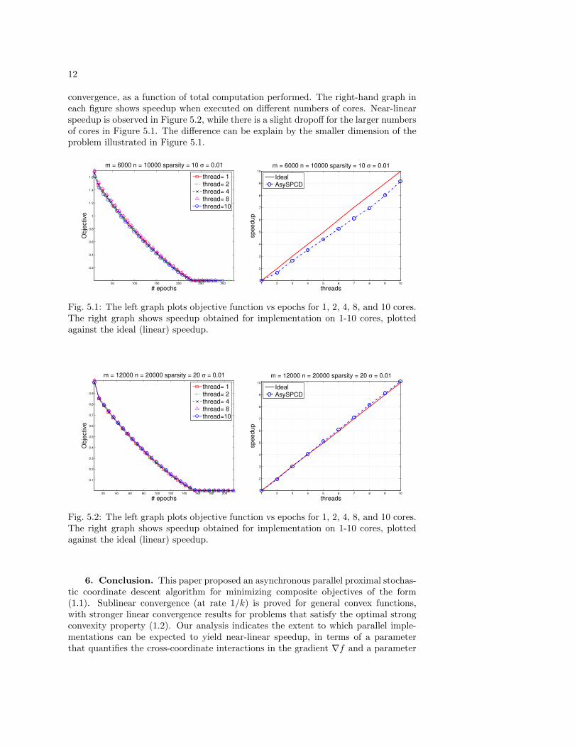
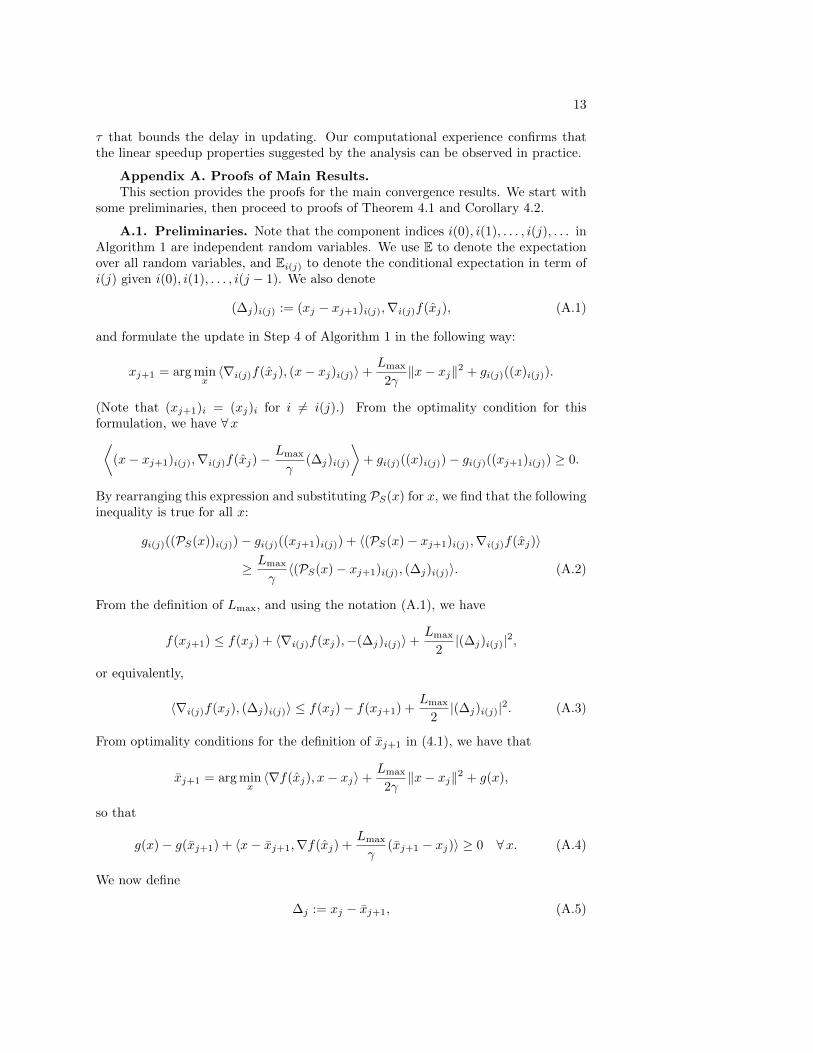
For the plots in Figures 5.1 and 5.2, we choose σ = 0.01 with m = 6000, n =10000, and s = 10 in Figure 5.1 and m = 12000, n = 20000, and s = 20 in Figure 5.2.We set λ = 20

√m log(n)σ (a value of the order of

√m log(n)σ is suggested by

compressed sensing theory) and the steplength γ is set as 1 in both figures. Note thatin both cases, we can estimate the ratio of Lres/Lmax roughly by 1 +

√n/m ≈ 2.3 as

suggested in the end of Section 1. Our final computed values of x x have nonzeros inthe same locations as the chosen solution x∗, though the values differ, because of thenoise in b.

The left-hand graph in each figure indicates the number of threads / cores andplots objective function value vs epoch count, where one epoch is equivalent to niterations. Note that the curves are almost overlaid, indicating that the total work-load required for AsySPCD is almost independent of the number of cores used in thecomputation. This observation validates our result in Corollary 4.2, which indicatesthat provided τ is below a certain threshold, it does not seriously affect the rate of

12

convergence, as a function of total computation performed. The right-hand graph ineach figure shows speedup when executed on different numbers of cores. Near-linearspeedup is observed in Figure 5.2, while there is a slight dropoff for the larger numbersof cores in Figure 5.1. The difference can be explain by the smaller dimension of theproblem illustrated in Figure 5.1.

50 100 150 200 250 300

0.2

0.4

0.6

0.8

1

1.2

1.4

1.6

m = 6000 n = 10000 sparsity = 10 σ = 0.01

# epochs

Ob

jective

thread= 1thread= 2thread= 4thread= 8thread=10

1 2 3 4 5 6 7 8 9 101

2

3

4

5

6

7

8

9

10

m = 6000 n = 10000 sparsity = 10 σ = 0.01

threads

speedup

IdealAsySPCD

Fig. 5.1: The left graph plots objective function vs epochs for 1, 2, 4, 8, and 10 cores.The right graph shows speedup obtained for implementation on 1-10 cores, plottedagainst the ideal (linear) speedup.

20 40 60 80 100 120 140 160 180 200

0.1

0.2

0.3

0.4

0.5

0.6

0.7

0.8

0.9

1

m = 12000 n = 20000 sparsity = 20 σ = 0.01

# epochs

Ob

jective

thread= 1thread= 2thread= 4thread= 8thread=10

1 2 3 4 5 6 7 8 9 101

2

3

4

5

6

7

8

9

10

m = 12000 n = 20000 sparsity = 20 σ = 0.01

threads

speedup

IdealAsySPCD

Fig. 5.2: The left graph plots objective function vs epochs for 1, 2, 4, 8, and 10 cores.The right graph shows speedup obtained for implementation on 1-10 cores, plottedagainst the ideal (linear) speedup.

6. Conclusion. This paper proposed an asynchronous parallel proximal stochas-tic coordinate descent algorithm for minimizing composite objectives of the form(1.1). Sublinear convergence (at rate 1/k) is proved for general convex functions,with stronger linear convergence results for problems that satisfy the optimal strongconvexity property (1.2). Our analysis indicates the extent to which parallel imple-mentations can be expected to yield near-linear speedup, in terms of a parameterthat quantifies the cross-coordinate interactions in the gradient ∇f and a parameter

13

τ that bounds the delay in updating. Our computational experience confirms thatthe linear speedup properties suggested by the analysis can be observed in practice.

Appendix A. Proofs of Main Results.This section provides the proofs for the main convergence results. We start with

some preliminaries, then proceed to proofs of Theorem 4.1 and Corollary 4.2.

A.1. Preliminaries. Note that the component indices i(0), i(1), . . . , i(j), . . . inAlgorithm 1 are independent random variables. We use E to denote the expectationover all random variables, and Ei(j) to denote the conditional expectation in term ofi(j) given i(0), i(1), . . . , i(j − 1). We also denote

(∆j)i(j) := (xj − xj+1)i(j),∇i(j)f(xj), (A.1)

and formulate the update in Step 4 of Algorithm 1 in the following way:

xj+1 = arg minx〈∇i(j)f(xj), (x− xj)i(j)〉+

Lmax

2γ‖x− xj‖2 + gi(j)((x)i(j)).

(Note that (xj+1)i = (xj)i for i 6= i(j).) From the optimality condition for thisformulation, we have ∀x⟨

(x− xj+1)i(j),∇i(j)f(xj)−Lmax

γ(∆j)i(j)

⟩+ gi(j)((x)i(j))− gi(j)((xj+1)i(j)) ≥ 0.

By rearranging this expression and substituting PS(x) for x, we find that the followinginequality is true for all x:

gi(j)((PS(x))i(j))− gi(j)((xj+1)i(j)) + 〈(PS(x)− xj+1)i(j),∇i(j)f(xj)〉

≥ Lmax

γ〈(PS(x)− xj+1)i(j), (∆j)i(j)〉. (A.2)

From the definition of Lmax, and using the notation (A.1), we have

f(xj+1) ≤ f(xj) + 〈∇i(j)f(xj),−(∆j)i(j)〉+Lmax

2|(∆j)i(j)|2,

or equivalently,

〈∇i(j)f(xj), (∆j)i(j)〉 ≤ f(xj)− f(xj+1) +Lmax

2|(∆j)i(j)|2. (A.3)

From optimality conditions for the definition of xj+1 in (4.1), we have that

xj+1 = arg minx〈∇f(xj), x− xj〉+

Lmax

2γ‖x− xj‖2 + g(x),

so that

g(x)− g(xj+1) + 〈x− xj+1,∇f(xj) +Lmax

γ(xj+1 − xj)〉 ≥ 0 ∀x. (A.4)

We now define

∆j := xj − xj+1, (A.5)

14

and note that this definition is consistent with (∆j)i(j) defined in (A.1). It can beseen that

Ei(j)(‖xj+1 − xj‖2) =1

n‖xj+1 − xj‖2. (A.6)

Recalling that all indices in K(j) are sorted in the increasing order from smallest(oldest) iterate to largest (newest) iterate, we use K(j)t to denote the t-th smallestentry in K(j). We define

xj,T := xj +

T∑t=1

(xK(j)t+1 − xK(j)t).

We have the following relations:

xj = xj,0

xj = xj,|K(j)|

xj − xj =

|K(j)|−1∑t=0

(xj,t+1 − xj,t)

∇f(xj)−∇f(xj) =

|K(j)|−1∑t=0

(∇f(xj,t+1)−∇f(xj,t)).

Furthermore, we have

‖∇f(xj)−∇f(xj)‖ = ‖∇f(xj,0)−∇f(xj,|K(j)|)‖

=

∥∥∥∥∥∥|K(j)|−1∑t=0

(∇f(xj,t)−∇f(xj,t+1))

∥∥∥∥∥∥≤|K(j)|−1∑t=0

‖∇f(xj,t)−∇f(xj,t+1)‖

≤ Lres

|K(j)|−1∑t=0

‖xj,t − xj,t+1‖

= Lres

|K(j)|∑t=1

‖xK(j)t − xK(j)t+1‖

= Lres

∑d∈K(j)

‖xd+1 − xd‖, (A.7)

where the second inequality holds because xj,t and xj,t+1 differ in only a single coor-dinate.

A.2. Proof of Theorem 4.1. Proof. We prove (4.5) by induction. First, notethat for any vectors a and b, we have

‖a‖2 − ‖b‖2 =2‖a‖2 − (‖a‖2 + ‖b‖2)

≤2‖a‖2 − 2〈a, b〉=2〈a, a− b〉≤2‖a‖‖b− a‖,

15

Thus for all j, we have

‖xj−1 − xj‖2 − ‖xj − xj+1‖2 ≤ 2‖xj−1 − xj‖‖xj − xj+1 − xj−1 + xj‖. (A.8)

The second factor in the r.h.s. of (A.8) is bounded as follows:

‖xj − xj+1 − xj−1 + xj‖

=

∥∥∥∥xj − PΩ

(xj −

γ

Lmax∇f(xj)

)−(xj−1 − PΩ(xj−1 −

γ

Lmax∇f(xj−1))

)∥∥∥∥≤ ‖xj − xj−1‖+

∥∥∥∥PΩ

(xj −

γ

Lmax∇f(xj)

)− PΩ

(xj−1 −

γ

Lmax∇f(xj−1)

)∥∥∥∥≤ 2‖xj − xj−1‖+

γ

Lmax‖∇f(xj)−∇f(xj−1)‖

(by the nonexpansive property of PΩ)

= 2‖xj − xj−1‖+γ

Lmax‖∇f(xj)−∇f(xj) +∇f(xj)−∇f(xj−1)

+∇f(xj−1)−∇f(xj−1)‖

≤ 2‖xj − xj−1‖+γ

Lmax

(‖∇f(xj)−∇f(xj)‖+ ‖∇f(xj)−∇f(xj−1)‖

+ ‖∇f(xj−1)−∇f(xj−1)‖)

≤ (2 + Λγ) ‖xj − xj−1‖+γ

Lmax‖∇f(xj)−∇f(xj)‖

+γ

Lmax‖∇f(xj−1)−∇f(xj−1)‖

≤ (2 + Λγ) ‖xj − xj−1‖+ Λγ∑

d∈K(j)

‖xd − xd+1‖

+ Λγ∑

d∈K(j−1)

‖xd − xd+1‖ (from (A.7)) (A.9)

≤ (2 + Λγ) ‖xj − xj−1‖+ Λγ

j−1∑d=j−τ

‖xd − xd+1‖+ Λγ

j−2∑d=j−1−τ

‖xd − xd+1‖

≤ (2 + 2Λγ) ‖xj − xj−1‖+ 2Λγ

j−2∑d=j−1−τ

‖xd − xd+1‖, (A.10)

where the fourth inequality uses ‖∇f(xj) − ∇f(xj−1)‖ ≤ Lres‖xj − xj−1‖, since xjand xj−1 differ in just one component.

We set j = 1, and note that K(0) = ∅ and K(1) ⊂ 0. In this case, we obtain abound from (A.9)

‖x1 − x2 + x0 − x1‖ ≤ (2 + Λγ) ‖x1 − x0‖+ Λγ‖x1 − x0‖ = (2 + 2Λγ) ‖x1 − x0‖.

By substituting this bound in (A.8) and setting j = 1, and taking expectations, weobtain

E(‖x0 − x1‖2)− E(‖x1 − x2‖2) ≤ 2E(‖x0 − x1‖‖x1 − x2 − x0 + x1‖)≤ (4 + 4Λγ)E(‖x1 − x0‖‖x1 − x0‖). (A.11)

16

For any positive scalars µ1, µ2, and α, we have

µ1µ2 ≤1

2(αµ2

1 + α−1µ22). (A.12)

It follows that

E(‖xj − xj−1‖‖xj − xj−1‖) ≤1

2E(n1/2‖xj − xj−1‖2 + n−1/2‖xj − xj−1‖2)

=1

2E(n1/2Ei(j−1)(‖xj − xj−1‖2) + n−1/2‖xj − xj−1‖2)

=1

2E(n−1/2‖xj − xj−1‖2 + n−1/2‖xj − xj−1‖2) (from (A.6))

= n−1/2E‖xj − xj−1‖2. (A.13)

By taking j = 1 in (A.13), and substituting in (A.11), we obtain

E(‖x0 − x1‖2)− E(‖x1 − x2‖2) ≤ n−1/2 (4 + 4Λγ)E‖x1 − x0‖2,

which implies that

E(‖x0 − x1‖2) ≤(

1− 4 + 4γΛ√n

)−1

E(‖x1 − x2‖2) ≤ ρE(‖x1 − x2‖2).

To see the last inequality, one only needs to verify that

ρ−1 ≤ 1− 4 + 4γΛ√n

⇔ γ ≤√n(1− ρ−1)− 4

4Λ,

where the last inequality follows from the second bound for γ in (4.4). We have thusshown that (4.5) holds for j = 1.

To take the inductive step, we assume that show that (4.5) holds up to indexj − 1. We have for j − 1− τ ≤ d ≤ j − 2 and any β > 0 (using (A.12) again) that

E(‖xd − xd+1‖‖xj − xj−1‖)

≤ 1

2E(n1/2β‖xd − xd+1‖2 + n−1/2β−1‖xj − xj−1‖2)

=1

2E(n1/2βEi(d)(‖xd − xd+1‖2) + n−1/2β−1‖xj − xj−1‖2)

=1

2E(n−1/2β‖xd − xd+1‖2 + n−1/2β−1‖xj − xj−1‖2) (from (A.6))

≤ 1

2E(n−1/2βρj−1−d‖xj−1 − xj‖2 + n−1/2β−1‖xj − xj−1‖2)

(by the inductive hypothesis).

Thus by setting β = ρ(d+1−j)/2, we obtain

E(‖xd − xd+1‖‖xj − xj−1‖) ≤ρ(j−1−d)/2

n1/2E(‖xj − xj−1‖2

). (A.14)

17

By substituting (A.10) into (A.8) and taking expectation on both sides of (A.8),we obtain

E(‖xj−1 − xj‖2)− E(‖xj − xj+1‖2)

≤2E(‖xj − xj−1‖‖xj − xj+1 + xj − xj−1‖)

≤2E

‖xj − xj−1‖

(2 + 2Λγ) ‖xj − xj−1‖+ 2Λγ

j−2∑d=j−1−τ

‖xd − xd+1‖

= (4 + 4Λγ)E(‖xj − xj−1‖‖xj − xj−1‖) + 4Λγ

j−2∑d=j−1−τ

E(‖xj − xj−1‖‖xd − xd+1‖)

≤n−1/2(4 + 4Λγ)E(‖xj − xj−1‖2)

+ n−1/24ΛγE(‖xj−1 − xj‖2)

j−2∑d=j−1−τ

ρ(j−1−d)/2 (from (A.13) and (A.14))

≤n−1/2(4 + 4Λγ)E(‖xj − xj−1‖2) + n−1/24ΛγE(‖xj−1 − xj‖2)

τ∑t=1

ρt/2

=n−1/2 (4 + 4Λγ(1 + θ))E(‖xj−1 − xj‖2),

where the last equality follows from the definition of θ in (4.3). It follows that

E(‖xj−1 − xj‖2) ≤(

1− n−1/2 (4 + 4Λγ(1 + θ)))−1

E(‖xj − xj+1‖2)

≤ρE(‖xj − xj+1‖2).

To see the last inequality, one only needs to verify that

ρ−1 ≤ 1− 4 + 4γΛ(1 + θ)√n

⇔ γ ≤√n(1− ρ−1)− 4

4Λ(1 + θ),

and the last inequality is true because of the upper bound of γ in (4.4). We have thusproved (4.5).

Next we will show the expectation of the objective F is monotonically decreasing.We have using the definition (A.1) that

Ei(j)F (xj+1) = Ei(j)[f(xj − (∆j)i(j)) + g(xj+1)

]≤ Ei(j)

[f(xj) + 〈∇i(j)f(xj), (xj+1 − xj)i(j)〉+

Lmax

2‖(xj+1 − xj)i(j)‖2

+ gi(j)((xj+1)i(j)) +∑l 6=i(j)

gl((xj+1)l)

]

= Ei(j)

[f(xj) + 〈∇i(j)f(xj), (xj+1 − xj)i(j)〉+

Lmax

2‖(xj+1 − xj)i(j)‖2

+ gi(j)((xj+1)i(j)) +∑l 6=i(j)

gl((xj)l)

]

= f(xj) +n− 1

ng(xj) + n−1

(〈∇f(xj), xj+1 − xj〉+

Lmax

2‖xj+1 − xj‖2 + g(xj+1)

)

18

where we used Since Ei(j)∑l 6=i(j) gl(xj)l = n−1

n g(xj) in the last equality. By addingand subtracting a term involving xj , we obtain

Ei(j)F (xj+1)

=F (xj) +1

n

(〈∇f(xj), xj+1 − xj〉+

Lmax

2‖xj+1 − xj‖2 + g(xj+1)− g(xj)

)+

1

n〈∇f(xj)−∇f(xj), xj+1 − xj〉

≤F (xj) +1

n

(Lmax

2‖xj+1 − xj‖2 −

Lmax

γ‖xj+1 − xj‖2

)+

1

n〈∇f(xj)−∇f(xj), xj+1 − xj〉 (from (A.4) with x = xj)

=F (xj)−(

1

γ− 1

2

)Lmax

n‖xj+1 − xj‖2 +

1

n〈∇f(xj)−∇f(xj), xj+1 − xj〉. (A.15)

Consider the expectation of the last term on the right-hand side of this expression.We have

E〈∇f(xj)−∇f(xj), xj+1 − xj〉≤ E (‖∇f(xj)−∇f(xj)‖‖xj+1 − xj‖)

≤ LresE

∑d∈K(j)

‖xd+1 − xd‖‖xj+1 − xj‖

(from (A.7))

≤ Lres

j−1∑d=j−τ

ρ(j−d)/2

n1/2E(‖xj − xj+1‖2) (from (A.14) replace “j” by “j + 1”)

≤ n−1/2LresθE(‖xj − xj+1‖2) (from (4.3)) (A.16)

By taking expectations on both sides of (A.15) and substituting (A.16), we obtain

EF (xj+1) ≤ EF (xj)−1

n

((1

γ− 1

2

)Lmax −

Lresθ

n1/2

)E‖xj+1 − xj‖2.

To see(

1γ −

12

)Lmax − Lresθ

n1/2 ≥ 0 or equivalently(

1γ −

12

)− Λθ

n1/2 ≥ 0, we note from

(4.3) and (4.4) that

γ−1 ≥ ψ ≥ 1

2+

Λθ√n.

Therefore, we have proved the monotonicity of the expectation of the objectives, thatis,

EF (xj+1) ≤ EF (xj), j = 0, 1, 2, . . . . (A.17)

Next we prove the sublinear convergence rate for the constrained smooth convex

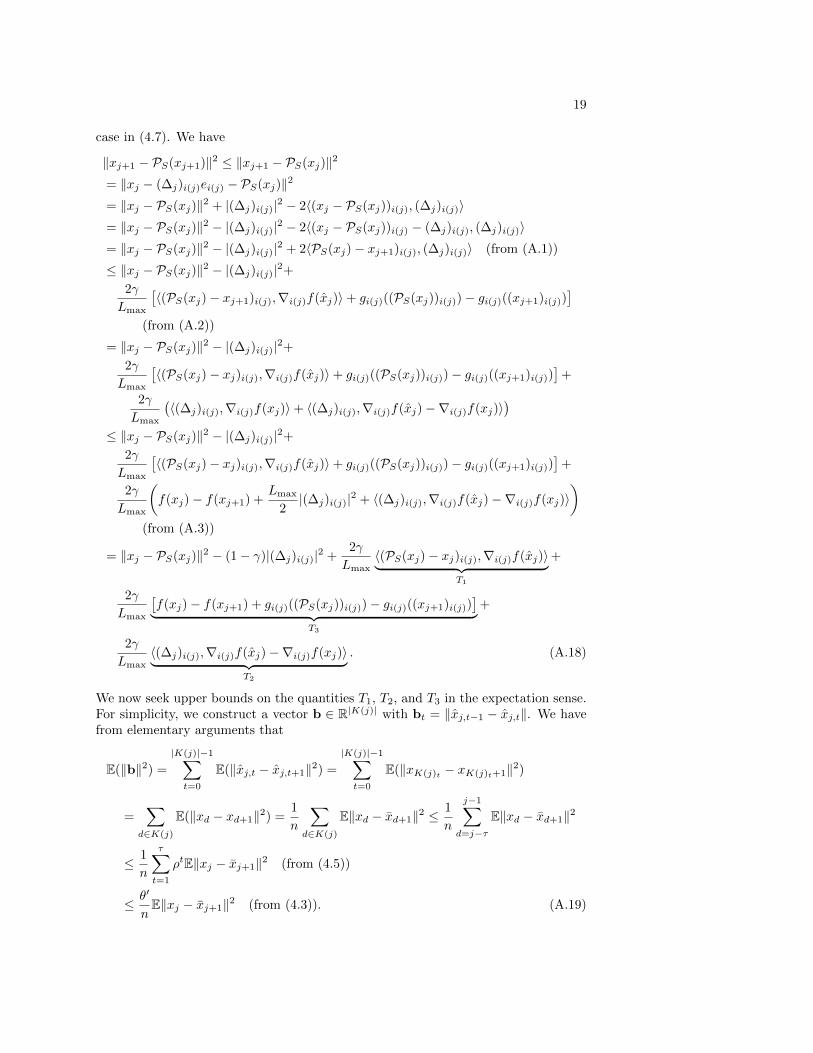
19

case in (4.7). We have

‖xj+1 − PS(xj+1)‖2 ≤ ‖xj+1 − PS(xj)‖2

= ‖xj − (∆j)i(j)ei(j) − PS(xj)‖2

= ‖xj − PS(xj)‖2 + |(∆j)i(j)|2 − 2〈(xj − PS(xj))i(j), (∆j)i(j)〉= ‖xj − PS(xj)‖2 − |(∆j)i(j)|2 − 2〈(xj − PS(xj))i(j) − (∆j)i(j), (∆j)i(j)〉= ‖xj − PS(xj)‖2 − |(∆j)i(j)|2 + 2〈PS(xj)− xj+1)i(j), (∆j)i(j)〉 (from (A.1))

≤ ‖xj − PS(xj)‖2 − |(∆j)i(j)|2+

2γ

Lmax

[〈(PS(xj)− xj+1)i(j),∇i(j)f(xj)〉+ gi(j)((PS(xj))i(j))− gi(j)((xj+1)i(j))

](from (A.2))

= ‖xj − PS(xj)‖2 − |(∆j)i(j)|2+

2γ

Lmax

[〈(PS(xj)− xj)i(j),∇i(j)f(xj)〉+ gi(j)((PS(xj))i(j))− gi(j)((xj+1)i(j))

]+

2γ

Lmax

(〈(∆j)i(j),∇i(j)f(xj)〉+ 〈(∆j)i(j),∇i(j)f(xj)−∇i(j)f(xj)〉

)≤ ‖xj − PS(xj)‖2 − |(∆j)i(j)|2+

2γ

Lmax

[〈(PS(xj)− xj)i(j),∇i(j)f(xj)〉+ gi(j)((PS(xj))i(j))− gi(j)((xj+1)i(j))

]+

2γ

Lmax

(f(xj)− f(xj+1) +

Lmax

2|(∆j)i(j)|2 + 〈(∆j)i(j),∇i(j)f(xj)−∇i(j)f(xj)〉

)(from (A.3))

= ‖xj − PS(xj)‖2 − (1− γ)|(∆j)i(j)|2 +2γ

Lmax〈(PS(xj)− xj)i(j),∇i(j)f(xj)〉︸ ︷︷ ︸

T1

+

2γ

Lmax

[f(xj)− f(xj+1) + gi(j)((PS(xj))i(j))− gi(j)((xj+1)i(j))

]︸ ︷︷ ︸T3

+

2γ

Lmax〈(∆j)i(j),∇i(j)f(xj)−∇i(j)f(xj)〉︸ ︷︷ ︸

T2

. (A.18)

We now seek upper bounds on the quantities T1, T2, and T3 in the expectation sense.For simplicity, we construct a vector b ∈ R|K(j)| with bt = ‖xj,t−1 − xj,t‖. We havefrom elementary arguments that

E(‖b‖2) =

|K(j)|−1∑t=0

E(‖xj,t − xj,t+1‖2) =

|K(j)|−1∑t=0

E(‖xK(j)t − xK(j)t+1‖2)

=∑

d∈K(j)

E(‖xd − xd+1‖2) =1

n

∑d∈K(j)

E‖xd − xd+1‖2 ≤1

n

j−1∑d=j−τ

E‖xd − xd+1‖2

≤ 1

n

τ∑t=1

ρtE‖xj − xj+1‖2 (from (4.5))

≤ θ′

nE‖xj − xj+1‖2 (from (4.3)). (A.19)

20

For the expectation of T1, defined in (A.18), we have

E(T1) = E((PS(xj)− xj)i(j)∇i(j)f(xj)

)= n−1E〈PS(xj)− xj ,∇f(xj)〉

= n−1E〈PS(xj)− xj ,∇f(xj)〉+ n−1E|K(j)|−1∑t=0

〈xj,t − xj,t+1,∇f(xj)〉

= n−1E〈PS(xj)− xj ,∇f(xj)〉

+ n−1E|K(j)|−1∑t=0

(〈xj,t − xj,t+1,∇f(xj,t)〉+ 〈xj,t − xj,t+1,∇f(xj)−∇f(xj,t)〉)

≤ n−1E(f∗j − f(xj))

+ n−1E|K(j)|−1∑t=0

(f(xj,t)− f(xj,t+1) +

Lmax

2‖xj,t − xj,t+1‖2

)

+ n−1E|K(j)|−1∑t=0

〈xj,t − xj,t+1,∇f(xj)−∇f(xj,t)〉 (from (1.3))

= n−1E(f∗j − f(xj)) +Lmax

2nE‖b‖2

+ n−1E|K(j)|−1∑t=0

〈xj,t − xj,t+1,∇f(xj)−∇f(xj,t)〉

= n−1E(f∗j − f(xj)) +Lmax

2nE‖b‖2

+ n−1E|K(j)|−1∑t=0

⟨xj,t − xj,t+1,

t−1∑t′=0

∇f(xj,t′)−∇f(xj,t′+1)

⟩

≤ n−1E(f∗j − f(xj)) +Lmax

2nE‖b‖2

+ n−1E|K(j)|−1∑t=0

Lmax

(‖xj,t − xj,t+1‖

t−1∑t′=0

‖xj,t′ − xj,t′+1‖

)

= n−1E(f∗j − f(xj)) +Lmax

2nE‖b‖2 + n−1LmaxE

|K(j)|−1∑t=0

(bt+1

t−1∑t′=0

bt′+1

)

= n−1E(f∗j − f(xj)) +Lmax

2nE‖b‖2 +

Lmax

2nE(‖b‖21 − ‖b‖2)

= n−1E(f∗j − f(xj)) +Lmax

2nE(‖b‖21)

≤ n−1E(f∗j − f(xj)) +Lmaxτ

2nE(‖b‖2) (since ‖b‖1 ≤

√|K(j)|‖b‖ ≤

√τ‖b‖)

≤ n−1E(f∗j − f(xj)) +Lmaxτθ

′

2n2E(‖xj − xj+1‖2) (from (A.19)). (A.20)

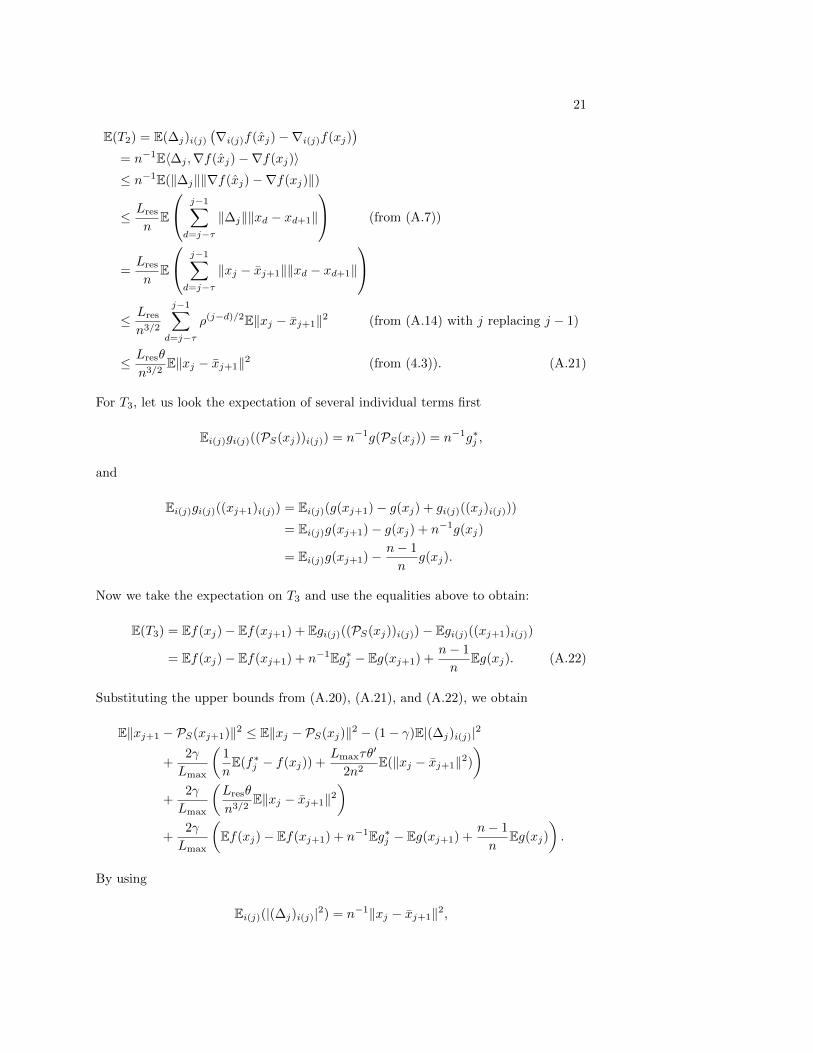
For the expectation of T2, we have

21

E(T2) = E(∆j)i(j)(∇i(j)f(xj)−∇i(j)f(xj)

)= n−1E〈∆j ,∇f(xj)−∇f(xj)〉≤ n−1E(‖∆j‖‖∇f(xj)−∇f(xj)‖)

≤ Lres

nE

j−1∑d=j−τ

‖∆j‖‖xd − xd+1‖

(from (A.7))

=Lres

nE

j−1∑d=j−τ

‖xj − xj+1‖‖xd − xd+1‖

≤ Lres

n3/2

j−1∑d=j−τ

ρ(j−d)/2E‖xj − xj+1‖2 (from (A.14) with j replacing j − 1)

≤ Lresθ

n3/2E‖xj − xj+1‖2 (from (4.3)). (A.21)

For T3, let us look the expectation of several individual terms first

Ei(j)gi(j)((PS(xj))i(j)) = n−1g(PS(xj)) = n−1g∗j ,

and

Ei(j)gi(j)((xj+1)i(j)) = Ei(j)(g(xj+1)− g(xj) + gi(j)((xj)i(j)))

= Ei(j)g(xj+1)− g(xj) + n−1g(xj)

= Ei(j)g(xj+1)− n− 1

ng(xj).

Now we take the expectation on T3 and use the equalities above to obtain:

E(T3) = Ef(xj)− Ef(xj+1) + Egi(j)((PS(xj))i(j))− Egi(j)((xj+1)i(j))

= Ef(xj)− Ef(xj+1) + n−1Eg∗j − Eg(xj+1) +n− 1

nEg(xj). (A.22)

Substituting the upper bounds from (A.20), (A.21), and (A.22), we obtain

E‖xj+1 − PS(xj+1)‖2 ≤ E‖xj − PS(xj)‖2 − (1− γ)E|(∆j)i(j)|2

+2γ

Lmax

(1

nE(f∗j − f(xj)) +

Lmaxτθ′

2n2E(‖xj − xj+1‖2)

)+

2γ

Lmax

(Lresθ

n3/2E‖xj − xj+1‖2

)+

2γ

Lmax

(Ef(xj)− Ef(xj+1) + n−1Eg∗j − Eg(xj+1) +

n− 1

nEg(xj)

).

By using

Ei(j)(|(∆j)i(j)|2) = n−1‖xj − xj+1‖2,

22

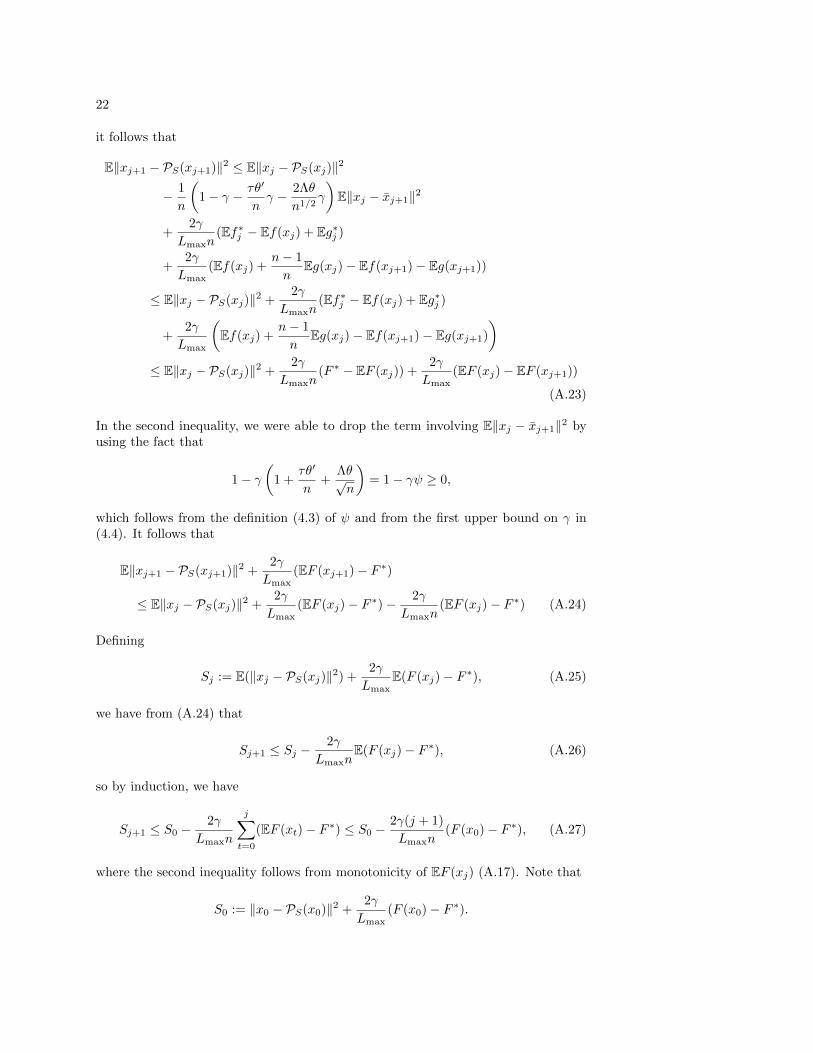
it follows that

E‖xj+1 − PS(xj+1)‖2 ≤ E‖xj − PS(xj)‖2

− 1

n

(1− γ − τθ′

nγ − 2Λθ

n1/2γ

)E‖xj − xj+1‖2

+2γ

Lmaxn(Ef∗j − Ef(xj) + Eg∗j )

+2γ

Lmax(Ef(xj) +

n− 1

nEg(xj)− Ef(xj+1)− Eg(xj+1))

≤ E‖xj − PS(xj)‖2 +2γ

Lmaxn(Ef∗j − Ef(xj) + Eg∗j )

+2γ

Lmax

(Ef(xj) +

n− 1

nEg(xj)− Ef(xj+1)− Eg(xj+1)

)≤ E‖xj − PS(xj)‖2 +

2γ

Lmaxn(F ∗ − EF (xj)) +

2γ

Lmax(EF (xj)− EF (xj+1))

(A.23)

In the second inequality, we were able to drop the term involving E‖xj − xj+1‖2 byusing the fact that

1− γ(

1 +τθ′

n+

Λθ√n

)= 1− γψ ≥ 0,

which follows from the definition (4.3) of ψ and from the first upper bound on γ in(4.4). It follows that

E‖xj+1 − PS(xj+1)‖2 +2γ

Lmax(EF (xj+1)− F ∗)

≤ E‖xj − PS(xj)‖2 +2γ

Lmax(EF (xj)− F ∗)−

2γ

Lmaxn(EF (xj)− F ∗) (A.24)

Defining

Sj := E(‖xj − PS(xj)‖2) +2γ

LmaxE(F (xj)− F ∗), (A.25)

we have from (A.24) that

Sj+1 ≤ Sj −2γ

LmaxnE(F (xj)− F ∗), (A.26)

so by induction, we have

Sj+1 ≤ S0 −2γ

Lmaxn

j∑t=0

(EF (xt)− F ∗) ≤ S0 −2γ(j + 1)

Lmaxn(F (x0)− F ∗), (A.27)

where the second inequality follows from monotonicity of EF (xj) (A.17). Note that

S0 := ‖x0 − PS(x0)‖2 +2γ

Lmax(F (x0)− F ∗).

23

By substituting the definition of Sj+1 into (A.27), we obtain

E‖xj+1 − PS(xj+1)‖2 +2γ

Lmax(EF (xj+1)− F ∗) +

2γ(j + 1)

Lmaxn(EF (xj+1)− F ∗)

≤ ‖x0 − PS(x0)‖2 +2γ

Lmax(F (x0)− F ∗).

The sublinear convergence expression (4.7) follows when we drop the (nonnegative)first term on the left-hand side of this expression, and rearrange.

Finally, we prove the linear convergence rate (4.6) for the optimally stronglyconvex case. All bounds proven above continue to hold, and we make use the optimalstrong convexity property in (1.2):

F (xj)− F ∗ ≥l

2‖xj − PS(xj)‖2.

By using this result together with some elementary manipulation, we obtain

F (xj)− F ∗ =

(1− Lmax

lγ + Lmax

)(F (xj)− F ∗) +

Lmax

lγ + Lmax(F (xj)− F ∗)

≥(

1− Lmax

lγ + Lmax

)(F (xj)− F ∗) +

Lmaxl

2(lγ + Lmax)‖xj − PS(xj)‖2

=Lmaxl

2(lγ + Lmax)

(‖xj − PS(xj)‖2 +

2γ

Lmax(F (xj)− F ∗)

). (A.28)

By taking expectations of both sides in this expression, and comparing with (A.25),we obtain

E(F (xj)− F ∗) ≥Lmaxl

2(lγ + Lmax)Sj .

By substituting into (A.26), we obtain

Sj+1 ≤Sj −(

2γ

Lmaxn

)Lmaxl

2(lγ + Lmax)Sj

=

(1− lγ

n(lγ + Lmax)

)Sj

≤(

1− lγ

n(lγ + Lmax)

)j+1

S0,

where the last inequality follows from induction over j. We obtain (4.6) by substitut-ing the definition (A.25) of Sj .

A.3. Proof of Corollary 4.2. Proof. Note that for ρ defined by (4.9), andusing (4.8), we have

ρ(1+τ)/2 =

(1 +

4eΛ(τ + 1)√n

)1+τ

=

(1 +4eΛ(τ + 1)√

n

) √n

4eΛ(τ+1)

4eΛ(τ+1)2√

n

≤ e4eΛ(τ+1)2√

n ≤ e. (A.29)

24

Thus from the definition of ψ (4.3), we have that

ψ = 1 +τθ′

n+

Λθ√n

≤ 1 +τ2ρτ

n+

Λτρτ/2√n

(from θ =

τ∑t=1

ρt/2 ≤ τρτ/2 and θ′ =

τ∑t=1

ρt ≤ τρτ)

≤ 1 +τ2e2

n+

Λτe√n

(from (A.29))

≤ 1 +1

16+

1

4≤ 2,

where for the second-past inequality we used (4.8) to obtain

Λτe√n≤ Λτe

4eΛ(τ + 1)2≤ 1

4,

τ2e2

n=

(τe√n

)2

≤(

Λτe√n

)≤ 1

16.

Thus, the steplength parameter choice γ = 1/2 satisfies the first bound in (4.4). Toshow that the second bound in (4.4) holds also, we have

√n(1− ρ−1)− 4

4(1 + θ)Λ

≥√n(1− ρ−1)

4(1 + θ)Λ− 1

2(from θ ≥ 1 and Λ ≥ 1)

≥√n(1− ρ−1/2)

4(1 + θ)Λ− 1

2

≥√n(ρ1/2 − 1)

4(1 + θ)ρ1/2Λ− 1

2

≥√n(ρ1/2 − 1)

4(τ + 1)ρ(τ+1)/2Λ− 1

2

(from (1 + θ)ρ

12 ≤ (1 + τρτ/2)ρ1/2 ≤ (1 + τ)ρ(τ+1)/2

)≥ 4eΛ(τ + 1)

4e(τ + 1)Λ− 1

2(from (4.9) and (A.29))

≥ 1− 1

2=

1

2.

We can thus set γ = 1/2, and by substituting this choice into (4.6), we obtain (4.10).We obtain (4.11) by making the same substitution into (4.7).

REFERENCES

[1] A. Agarwal and J. C. Duchi, Distributed delayed stochastic optimization, in Proceedings ofthe Conference on Decision and Control, 2012, pp. 5451–5452.

[2] M. Anitescu, Degenerate nonlinear programming with a quadratic growth condition, SIAMJournal on Optimization, 10 (2000), pp. 1116–1135.

[3] H. Avron, A. Druinsky, and A. Gupta, Revisiting asynchronous linear solvers: Provableconvergence rate through randomization, in Proceedings of the IEEE International Paralleland Distributed Processing Symposium, May 2014.

[4] A. Beck and M. Teboulle, A fast iterative shrinkage-thresholding algorithm for linear inverseproblems, SIAM Journal on Imaging Sciences, 2 (2009), pp. 183–202.

[5] A. Beck and L. Tetruashvili, On the convergence of block coordinate descent type methods,SIAM Journal on Optimization, 23 (2013), pp. 2037–2060.

25

[6] D. P. Bertsekas and J. N. Tsitsiklis, Parallel and Distributed Computation: NumericalMethods, Prentice Hall, 1989.

[7] S. Boyd, N. Parikh, E. Chu, B. Peleato, and J. Eckstein, Distributed optimization andstatistical learning via the alternating direction method of multipliers, Foundations andTrends in Machine Learning, 3 (2011), pp. 1–122.

[8] J. K. Bradley, A. Kyrola, D. Bickson, and C. Guestrin, Parallel coordinate descent forL1-regularized loss minimization, in International Conference on Machine Learning, 2011.

[9] C. Cortes and V. Vapnik, Support vector networks, Machine Learning, (1995), pp. 273–297.[10] A. Cotter, O. Shamir, N. Srebro, and K. Sridharan, Better mini-batch algorithms via ac-

celerated gradient methods, in Advances in Neural Information Processing Systems, vol. 24,2011, pp. 1647–1655.

[11] J. C. Duchi, A. Agarwal, and M. J. Wainwright, Dual averaging for distributed optimiza-tion: Convergence analysis and network scaling, IEEE Transactions on Automatic Control,57 (2012), pp. 592–606.

[12] L. Elsner, I. Koltracht, and M. Neumann, Convergence of sequential and asyn-chronous paracontractions nonlinear paracontractuions, Numerische Mathematik, 62(1992), pp. 305–316.

[13] O. Fercoq and P. Richtarik, Accelerated, parallel, and proximal coordinate descent, technicalreport, School of Mathematics, University of Edinburgh, 2013. arXiv: 1312.5799.

[14] , Smooth minimization of nonsmooth functions by parallel coordinate descent, technicalreport, School of Mathematics, University of Edinburgh, 2013. arXiv:1309.5885.

[15] M. C. Ferris and O. L. Mangasarian, Parallel variable distribution, SIAM Journal on Op-timization, 4 (1994), pp. 815–832.

[16] A. Frommer and D. B. Szyld, On asynchronous iterations, Journal of Computational andApplied Mathematics, 123 (2000), pp. 201–216.

[17] D. Goldfarb and S. Ma, Fast multiple-splitting algorithms for convex optimization, SIAMJournal on Optimization, 22 (2012), pp. 533–556.

[18] A. J. Hoffman, On approximate solutions of systems of linear inequalities, Journal of Researchof the National Bureau of Standards, 49 (1952), pp. 263–265.

[19] M. Lai and W. Yin, Augmented L1 and nuclear-norm models with a globally linearly conver-gent algorithm, SIAM Journal on Imaging Sciences, 6 (2013), pp. 1059–1091.

[20] J. Liu, S. J. Wright, C. Re, V. Bittorf, and S. Sridhar, An asynchronous parallel stochasticcoordinate descent algorithm, technical report, Computer Sciences Department, Universityof Wisconsin-Madison, February 2014. arXiv: 1311.1873.

[21] J. Liu, S. J. Wright, and S. Sridhar, An asynchronous parallel randomized Kaczmarz algo-rithm, technical report, Computer Sciences Department, University of Wisconsin-Madison,2014. arXiv: 1401.4780.

[22] Z. Lu and L. Xiao, On the complexity analysis of randomized block-coordinate descent methods,Technical Report MSR-TR-2013-53, Microsoft Research, May 2013. arXiv:1305.4723.

[23] Z.-Q. Luo and P. Tseng, On the convergence of the coordinate descent method for convexdifferentiable minimization, Journal of Optimization Theory and Applications, 72 (1992),pp. 7–35.

[24] O. L. Mangasarian, Parallel gradient distribution in unconstrained optimization, SIAM Jour-nal on Optimization, 33 (1995), pp. 916–1925.

[25] I. Necoara and D. Clipici, Efficient parallel coordinate descent algorithm for convex op-timization problems with separable constraints: application to distributed MPC, techni-cal report, Automation and Systems Engineering Department, University PolitechnicaBucharest, 2013. arXiv: 1302.3092.

[26] I. Necoara and A. Patrascu, A random coordinate descent algorithm for optimization prob-lems with composite objective function and linear coupled constraints, technical report, Au-tomation and Systems Engineering Department, University Politechnica Bucharest, 2013.arXiv: 1302.3074.

[27] A. Nemirovski, A. Juditsky, G. Lan, and A. Shapiro, Robust stochastic approximationapproach to stochastic programming, SIAM Journal on Optimization, 19 (2009), pp. 1574–1609.

[28] Y. Nesterov, Introductory Lectures on Convex Optimization: A Basic Course, Kluwer Aca-demic Publishers, 2004.

[29] , Efficiency of coordinate descent methods on huge-scale optimization problems, SIAMJournal on Optimization, 22 (2012), pp. 341–362.

[30] F. Niu, B. Recht, C. Re, and S. J. Wright, Hogwild: A lock-free approach to parallelizingstochastic gradient descent, Advances in Neural Information Processing Systems, 24 (2011),pp. 693–701.

26

[31] Z. Peng, M. Yan, and W. Yin, Parallel and distributed sparse optimization, tech. report,Department of Mathematics, UCLA, 2013.

[32] P. Richtarik and M. Takac, Iteration complexity of randomized block-coordinate descentmethods for minimizing a composite function, Mathematical Programing, Series A, (2012).(Published Online).

[33] , Parallel coordinate descent methods for big data optimization, technical report, Math-ematics Department, University of Edinburgh, 2012. arXiv: 1212.0873.

[34] C. Scherrer, A. Tewari, M. Halappanavar, and D. Haglin, Feature clustering for accel-erating parallel coordinate descent, in Advances in Neural Information Processing, vol. 25,2012, pp. 28–36.

[35] S. Shalev-Shwartz and T. Zhang, Accelerated mini-batch stochastic dual coordinate as-cent, in Advances in Neural Information Processing Systems, C. J. C. Burges, L. Bottou,M. Welling, Z. Ghahramani, and K. Q. Weinberger, eds., vol. 26, 2013, pp. 378–385.

[36] O. Shamir and T. Zhang, Stochastic gradient descent for non-smooth optimization: Conver-gence results and optimal averaging schemes, in Proceedings of the International Confer-ence on Machine Learning, 2013.

[37] S. Sridhar, V. Bittorf, J. Liu, C. Zhang, C. Re, and S. J. Wright, An approximateefficient solver for LP rounding, in Advances in Neural Information Processing Systems,vol. 26, 2013.

[38] P. Tseng, Convergence of a block coordinate descent method for nondifferentiable minimiza-tion, Journal of Optimization Theory and Applications, 109 (2001), pp. 475–494.

[39] P. Tseng and S. Yun, A coordinate gradient descent method for nonsmooth separable mini-mization, Mathematical Programming, Series B, 117 (2009), pp. 387–423.

[40] , A coordinate gradient descent method for linearly constrained smooth optimizationand support vector machines training, Computational Optimization and Applications, 47(2010), pp. 179–206.

[41] P.-W. Wang and C.-J. Lin, Iteration complexity of feasible descent methods for convex opti-mization, technical report, Department of Computer Science, National Taiwan University,2013.

[42] S. J. Wright, R. D. Nowak, and M. A. T. Figueiredo, Sparse reconstruction by separableapproximation, IEEE Transactions on Signal Processing, 57 (2009), pp. 2479–2493.