P.1

JAMES S. BethelWonjo Jung

Geomatics EngineeringSchool of Civil Engineering

Purdue UniversityAPR-30-2008

Sensor Modeling and Triangulation for an Airborne Three Line Scanner

< 2008 ASPRS Annual Conference >

P.2

Outline1. Introduction2.Dataset

– Camera Design– Flight and observations (3-OC Atlanta, GA)

3.Sensor Model4.Trajectory Model5.Pseudo Observation Equations6.Data Ajustment7. Implementation8.Results9.Conclusions10.Future plans

P.3

1. Introduction

MAIN OBJECTIVE

Developing an algorithm to recover orientation parameters for an airborne three line scanner

P.4

1. Introduction- Types of three line scanners

Lens

Linear arrays on the same focal plane

Three separate cameras

P.5

1. Introduction

nx

ny

Instantaneous gimbal rotation center

nf

flight trajectory

fx

fy ff

bx

bybf

fV

nV

bV

fLXYZ

''''''''''''''

gXYZ''''''''''''''

nLXYZ

''''''''''''''

bLXYZ

''''''''''''''

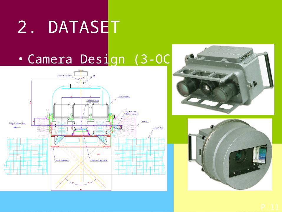
• While ADS40, TLS and JAS placed CCD arrays on the focal plane in a single optical system, 3-DAS-1 and 3-OC use three optical systems, rigidly fixed to each other.

• For this reason, we need to develop a photogrammetirc model for three different cameras moving together along a single flight trajectory

P.6

1. Introduction

• Parameters to be estimated– Exterior orientation parameters

• 6 parameters per an image line

– Additional external parameters• Translation vector between a gimbal center to perspective centers• Rotation angles between gimbal axis and sensor coordinate

systems

– Interior orientation parameters• Focal lengths• Principal points• Radial distortions

P.7

1. Introduction

• There have been two kinds of approaches.

– Reducing number of unknown parameters• Piece-wise polynomials

– Providing fictitious observations in addition to the real observations

• Stochastic models

P.8

1. Introduction

• Reducing number of unknown parameters– Piecewise polynomials

20 0 0 1 2

20 0 0 1 2

20 0 0 1 2

20 0 0 1 2

20 0 0 1 2

20 0 0 1 2

X X dX X x x t x t

Y Y dY Y y y t y t

Z Z dZ Z z z t z t

R R dR R r rt r t

P P dP P p p t p t

H H dH H h h t h t

given

estimated

1000×6=6000

3×6=18

P.9

1. Introduction

• Providing fictitious observations in addition to the real observations– 1st-Order Gauss-Markov Model

given

1 1

2 1

3 1

4 1

5 1

6 1

Conventional Pseudo Observation Equation

( ) ( ) 0

( ) ( ) 0

( ) ( ) 0

( ) ( ) 0

( ) ( ) 0

( ) ( ) 0

XL

YL

ZL

s

G L i L i

s

G L i L i

s

G L i L i

sG i i

sG i i

sG i i

F e X X

F e Y Y

F e Z Z

F e

F e

F e

estimated

observations

P.10

1. Introduction

• Self-calibration– Partial camera calibration information is provided.

• focal length, aperture ratio, shift of the distortion center, radial distortion

– Coordinates of projection center of the camera relative to the gimbal center is not measured. Just design values are provided.

– Need to refine some of the parameters

P.11

2. DATASET

• Camera Design (3-OC)

P.12

2. DATASETStrip ID Heading Altitude

2 E

5,500ft

3 W

4 E

5 W

6 S

8 N

9 S

10 N

11 S

10,500ft

12 N

13 S

14 N

15 E

16 W

17 E

18 W

: 20 GCPs

: 8Check points

2 3

4 5

6

8

9

10

11

12

13

14

15 16

17 18

P.13

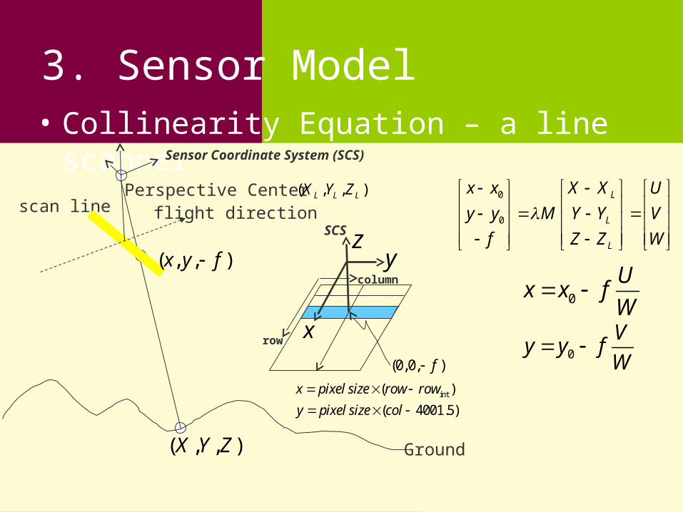
3. Sensor Model• Collinearity Equation – a line scanner

( , , )X Y Z Ground

scan linePerspective Center ( , , )L L LX Y Z

( , , )x y f

0

0

L

L

L

x x X X U

y y M Y Y V

f Z Z W

0

Ux x f

W

0

Vy y f

W

flight direction

Sensor Coordinate System (SCS)

row

column

x

yz

(0,0, )f

SCS

int( )

( 4001.5)

x pixel size row row

y pixel size col

P.14

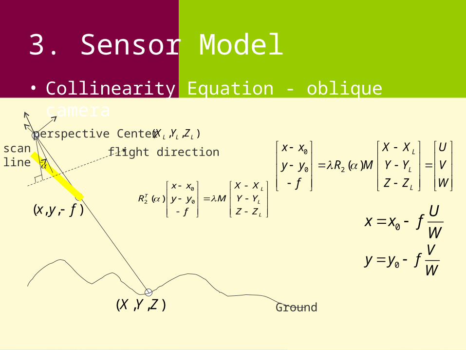
3. Sensor Model• Collinearity Equation - oblique camera

( , , )X Y Z Ground

scanline

perspective Center ( , , )L L LX Y Z

( , , )x y f

flight direction

0

2 0( )L

TL

L

x x X X

R y y M Y Y

f Z Z

0

0 2 ( )L

L

L

x x X X U

y y R M Y Y V

f Z Z W

0

Ux x f

W

0

Vy y f

W

P.15

3. Sensor Model• Collinearity in a three line scanner

flight directiongimbal center

plumb line

F

N

B 0

2 0

0

0

0

2 0

Forward Camera

( )

Nadir Camera

Backward Camera

( )

f fL

T f fL

f fL

n nL

n nL

n nL

b bL

T b bL

b bL

x x X X

R y y M Y Y

f Z Z

x x X X

y y M Y Y

f Z Z

x x X X

R y y M Y Y

f Z Z

three angles should be considered

P.16

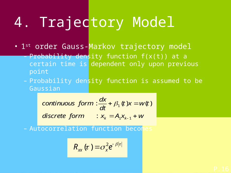
4. Trajectory Model

• 1st order Gauss-Markov trajectory model– Probability density function f(x(t)) at a certain time is

dependent only upon previous point– Probability density function is assumed to be Gaussian

– Autocorrelation function becomes

1

1 1

: ( ) ( )

: k k

dxcontinuous form t x w t

dtdiscrete form x A x w

2( )xx xR e

P.17

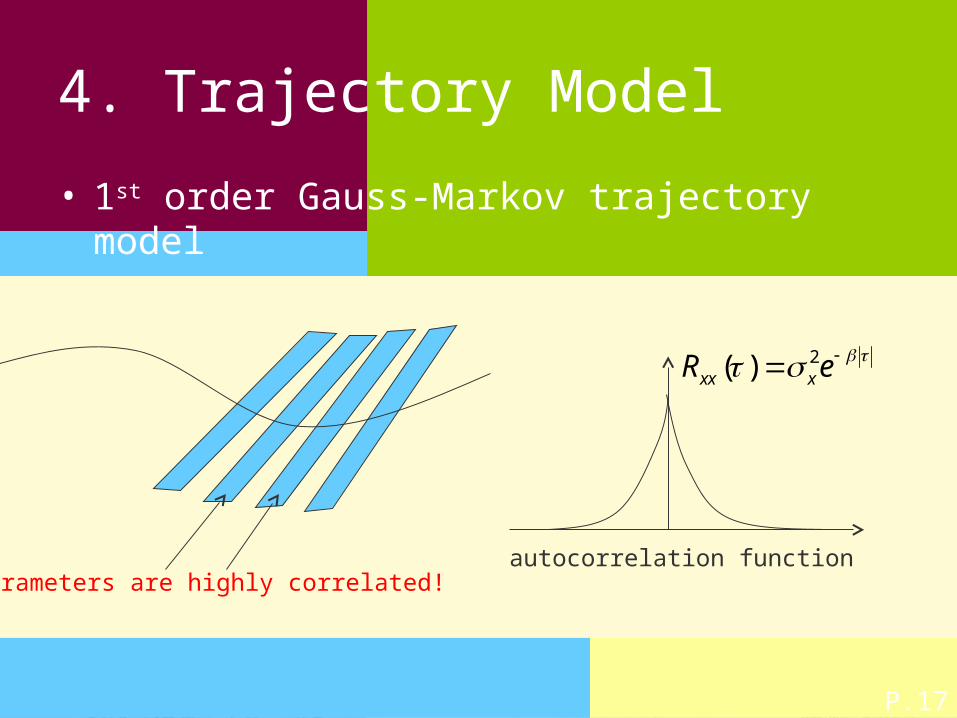
4. Trajectory Model

• 1st order Gauss-Markov trajectory model

Parameters are highly correlated!

2( )xx xR e

autocorrelation function

P.18

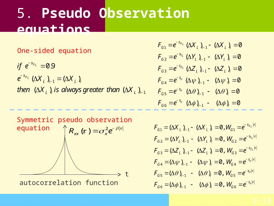
5. Pseudo Observation equations

1 1

2 1

3 1

4 1

5 1

6 1

( ) ( ) 0

( ) ( ) 0

( ) ( ) 0

( ) ( ) 0

( ) ( ) 0

( ) ( ) 0

XL

YL

ZL

s

G L i L i

s

G L i L i

s

G L i L i

sG i i

sG i i

sG i i

F e X X

F e Y Y

F e Z Z

F e

F e

F e

t

2( )xx xR e

autocorrelation function

One-sided equation

1

1

0.9

( ) ( )

( ) ( )

XL

XL

s

s

L i L i

L i L i

if e

e X X

then X is always greater than X

1 1 1

2 1 2

3 1 3

4 1 4

5 1 5

6 1 6

( ) ( ) 0,

( ) ( ) 0,

( ) ( ) 0,

( ) ( ) 0,

( ) ( ) 0,

( ) ( ) 0,

XL

YL

ZL

s

G L i L i G

s

G L i L i G

s

G L i L i G

sG i i G

sG i i G

sG i i G

F X X W e

F Y Y W e

F Z Z W e

F W e

F W e

F W e

Symmetric pseudo observation equation

P.19

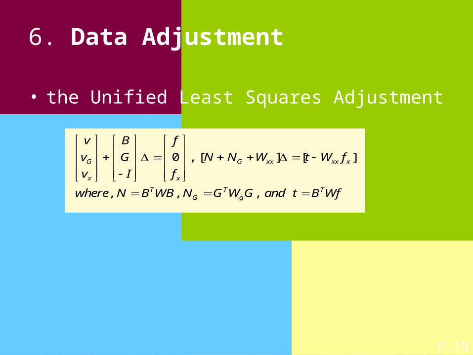
6. Data Adjustment

• the Unified Least Squares Adjustment

0 , [ ] [ ]

, , ,

G G xx xx x

x x

T T TG g

v B f

v G N N W t W f

v I f

where N B WB N G W G and t B Wf

P.20

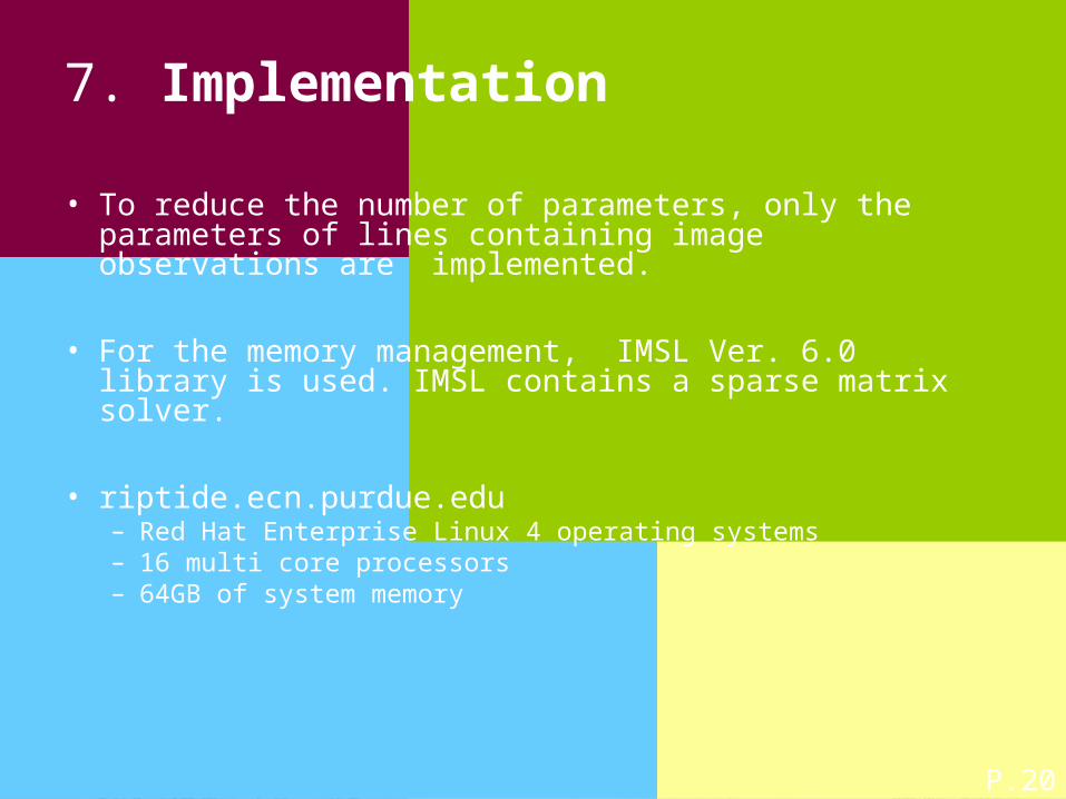
7. Implementation

• To reduce the number of parameters, only the parameters of lines containing image observations are implemented.

• For the memory management, IMSL Ver. 6.0 library is used. IMSL contains a sparse matrix solver.

• riptide.ecn.purdue.edu– Red Hat Enterprise Linux 4 operating systems – 16 multi core processors– 64GB of system memory

P.21

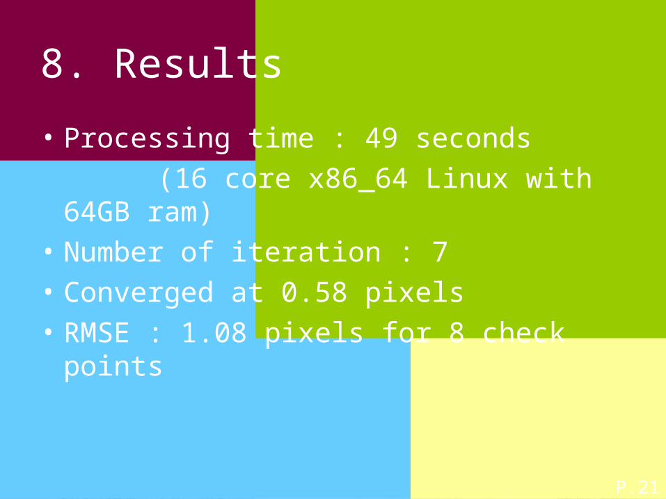
8. Results

• Processing time : 49 seconds

(16 core x86_64 Linux with 64GB ram)

• Number of iteration : 7

• Converged at 0.58 pixels

• RMSE : 1.08 pixels for 8 check points

P.22

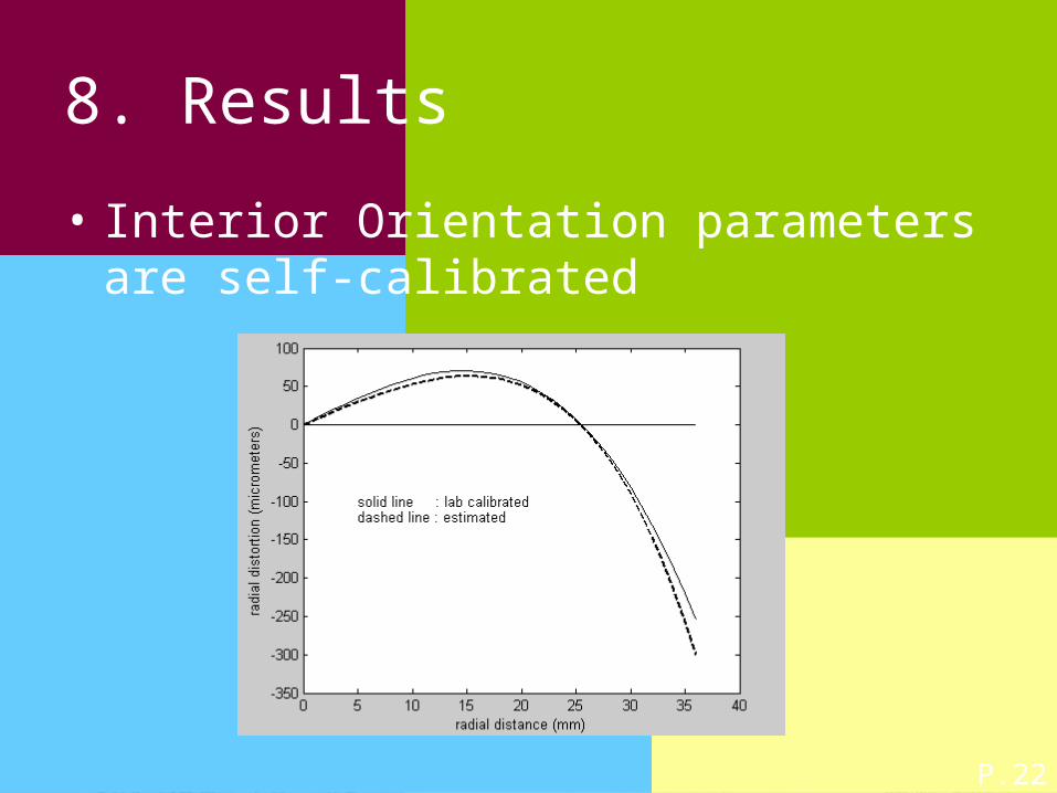
8. Results

• Interior Orientation parameters are self-calibrated

P.23

9. Conclusions

• We could successfully recover the orientation parameters using stochastic trajectory model

• Interior orientation parameters of three cameras can be refined through the self calibration process

P.24

9. Future Plans

• Analysis on the model properties

• Adding pass points

• Automated passpoints generation