Embed Size (px)
DESCRIPTION
P REDICTION O F F RONTOGENETICALLY F ORCED P RECIPITATION B ANDS. PETER C. BANACOS NWS / Storm Prediction Center WDTB Winter Weather Workshop IV Boulder, CO ~ 23 July 2003. O UTLINE. Frontogenesis …where it fits in the forecast process kinematics and dynamics of frontogenesis - PowerPoint PPT Presentation
Citation preview
PREDICTION OF FRONTOGENETICALLY FORCED
PRECIPITATION BANDS
PETER C. BANACOSNWS / Storm Prediction Center
WDTB Winter Weather Workshop IVBoulder, CO ~ 23 July 2003
OUTLINE
I. Frontogenesis …where it fits in the forecast process kinematics and dynamics of frontogenesis synoptic pattern recognition Case #1 – examine band formation
II. Mesoscale Banding Characteristics modulation by local wind profile col point aloft modulation by stability Case #2 – numerical model considerations
INGREDIENTS BASED
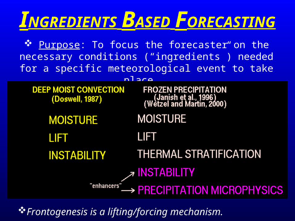
FORECASTING Purpose: To focus the forecaster on the necessary conditions (“ingredients”) needed for a specific
meteorological event to take place.
Frontogenesis is a lifting/forcing mechanism.
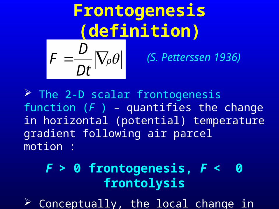
Frontogenesis (definition)
pDt
DF
The 2-D scalar frontogenesis function (F ) – quantifies the change in horizontal (potential) temperature gradient following air parcel motion :
F > 0 frontogenesis, F < 0 frontolysis
Conceptually, the local change in horizontal temperature gradient near an existing front, baroclinic zone, or feature as it moves.
(S. Petterssen 1936)
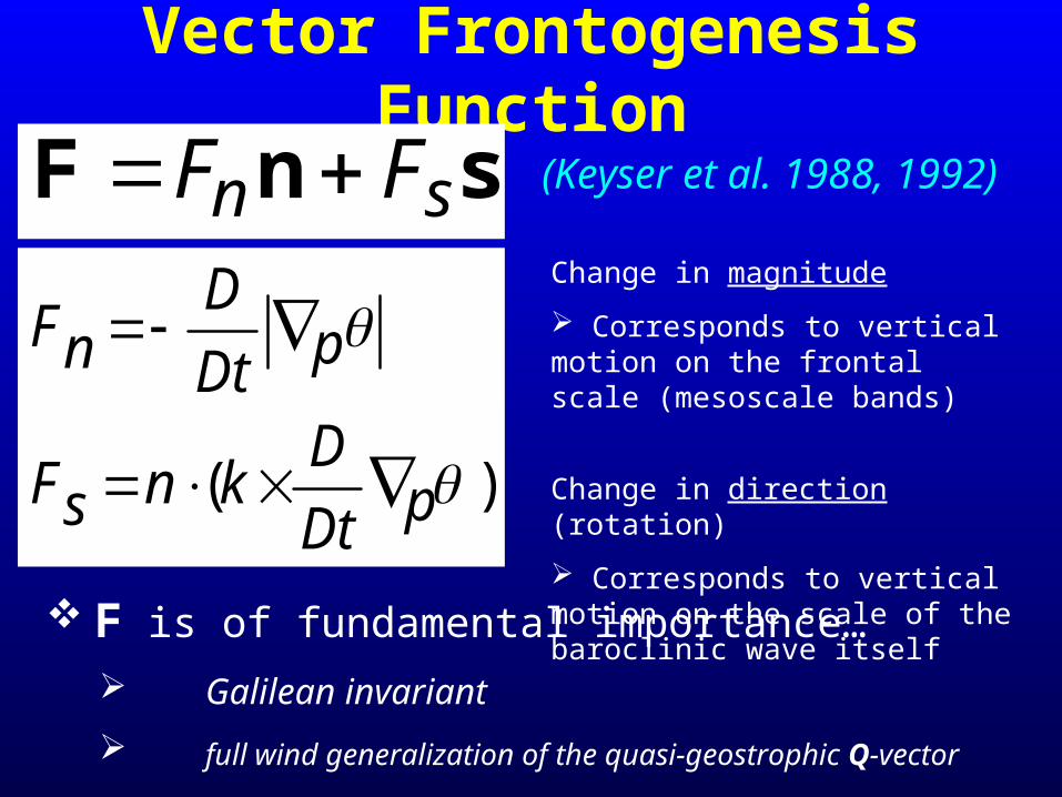
Vector Frontogenesis Function
(Keyser et al. 1988, 1992)
snF sn FF
)(
pDt
DknsF
pDt
DnF
Change in magnitude
Corresponds to vertical motion on the frontal scale (mesoscale bands)
Change in direction (rotation)
Corresponds to vertical motion on the scale of the baroclinic wave itself F is of fundamental importance…
Galilean invariant
full wind generalization of the quasi-geostrophic Q-vector
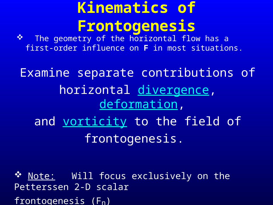
Kinematics of Frontogenesis
The geometry of the horizontal flow has a first-order influence on F in most situations.
Examine separate contributions ofhorizontal divergence, deformation,
and vorticity to the field offrontogenesis.
Note: Will focus exclusively on the Petterssen 2-D
scalar frontogenesis (Fn)
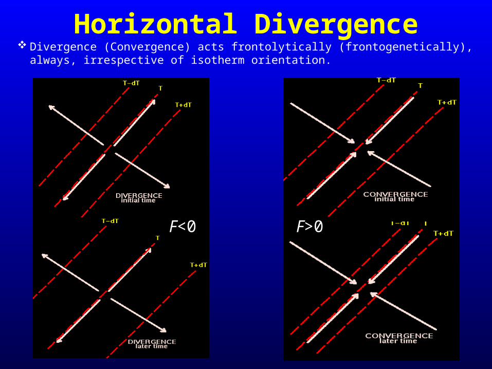
Horizontal Divergence Divergence (Convergence) acts frontolytically (frontogenetically),
always, irrespective of isotherm orientation.
F<0 F>0
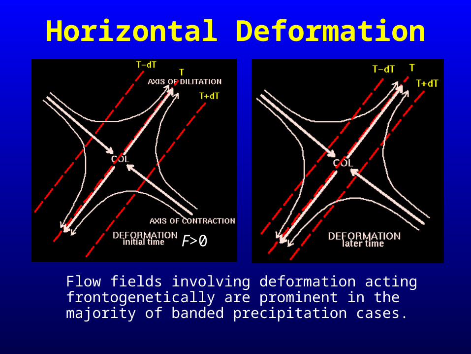
Horizontal Deformation
Flow fields involving deformation acting frontogenetically are prominent in the majority of banded precipitation cases.
F>0
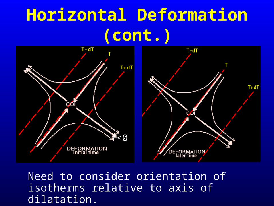
Horizontal Deformation (cont.)
F<0
Need to consider orientation of isotherms relative to axis of dilatation.

Vertical Vorticity
Pure vorticity acts to rotate isotherms, cannot tighten or weaken them.
F=0
Other Contributing Factors to
FrontogenesisThe kinematic field, and deformation in particular, plays the
most prominent role in the 2-D frontogenesis aloft.
Other processes such as diabatic heating and tilting effects may also contribute to frontogenesis.
Examples:differential solar heatingLatent heating with convective motions
(documented in coastal frontogenesis process).
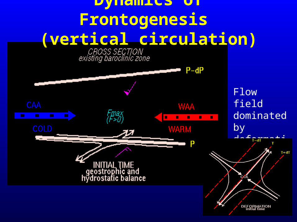
Dynamics of Frontogenesis
(vertical circulation)
Flow field dominated by deformation.

Dynamics of Frontogenesis (cont.)
Ageostrophic circulation develops as a response to increasing temperature gradient.
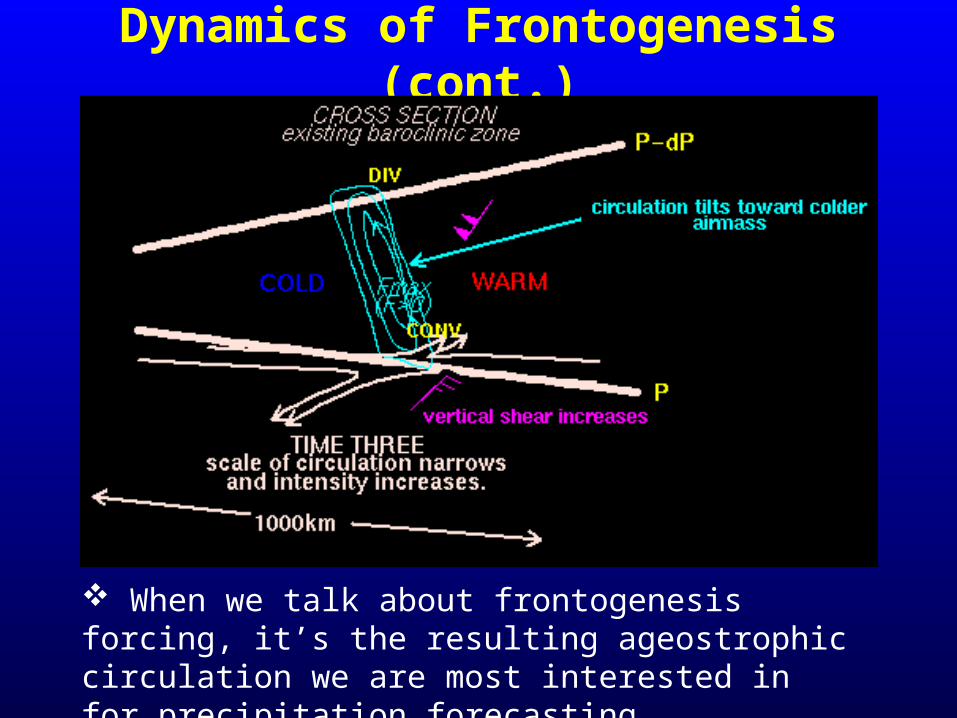
Dynamics of Frontogenesis (cont.)
When we talk about frontogenesis forcing, it’s the resulting ageostrophic circulation we are most interested in for precipitation forecasting.
Forecasting Applications
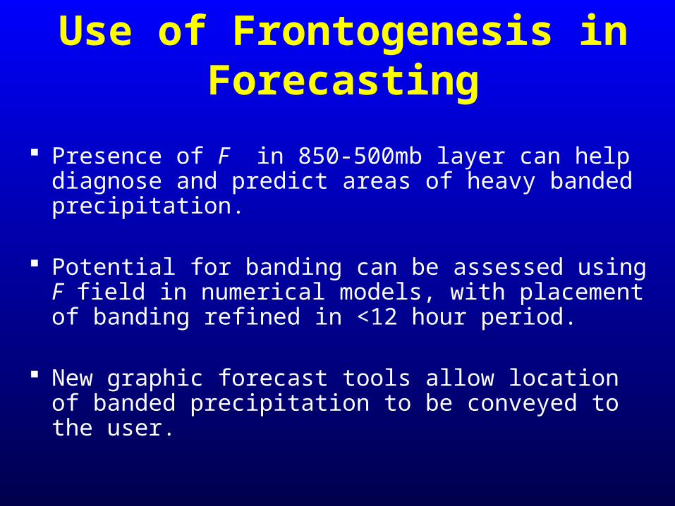
Use of Frontogenesis in Forecasting
Presence of F in 850-500mb layer can help diagnose and predict areas of heavy banded precipitation.
Potential for banding can be assessed using F field in numerical models, with placement of banding refined in <12 hour period.
New graphic forecast tools allow location of banded precipitation to be conveyed to the user.

Common Synoptic Patterns
TWO CLASSES OF BANDS: Bands associated with surface cyclogenesis Bands not associated with surface cyclogenesis
Forecast premise for mesoscale banding:
• Requires a strengthening baroclinic zone in the presence of sufficient moisture for precipitation (AND – for snow, the proper thermal stratification).
• Large-scale deformation zones are BY FAR AND AWAY the most common means of manifesting areas of frontogenesis within the 850-500mb layer.
• Does NOT require a strong surface cyclone, only a low-mid tropospheric baroclinic zone
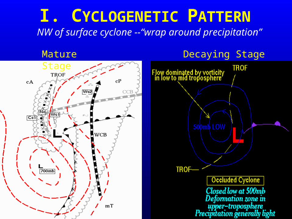
I. CYCLOGENETIC PATTERN
Mature Stage
Decaying Stage
NW of surface cyclone --“wrap around precipitation”
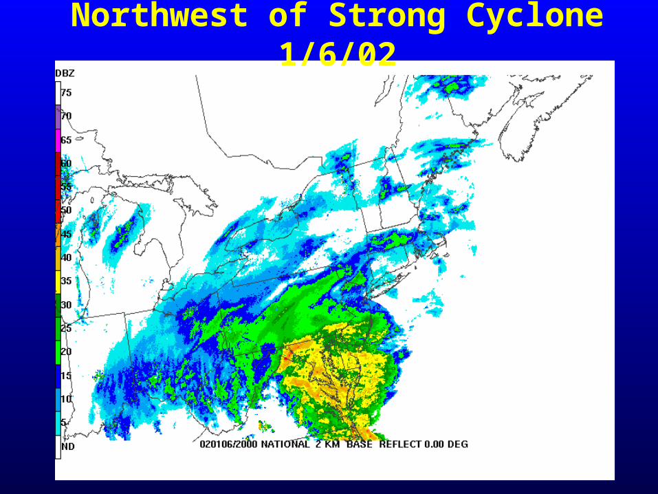
Northwest of Strong Cyclone 1/6/02
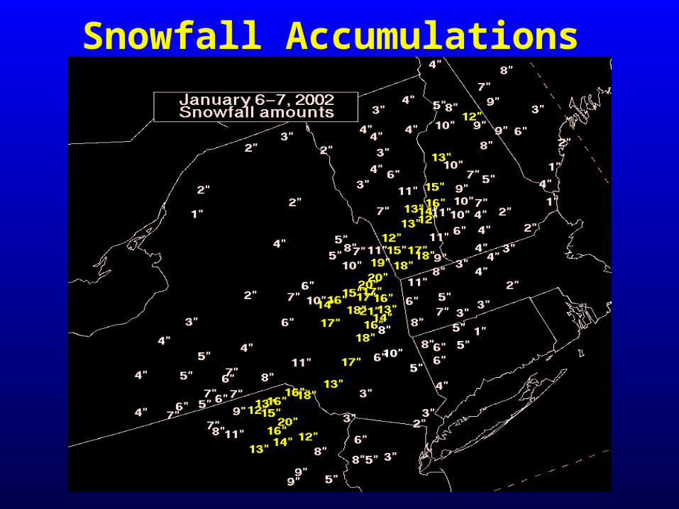
Snowfall Accumulations
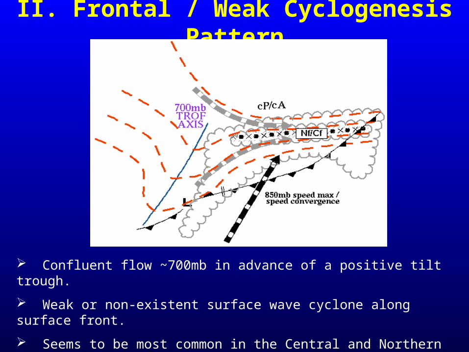
II. Frontal / Weak Cyclogenesis Pattern
Confluent flow ~700mb in advance of a positive tilt trough.
Weak or non-existent surface wave cyclone along surface front.
Seems to be most common in the Central and Northern Plains with quasi-stationary arctic boundaries.
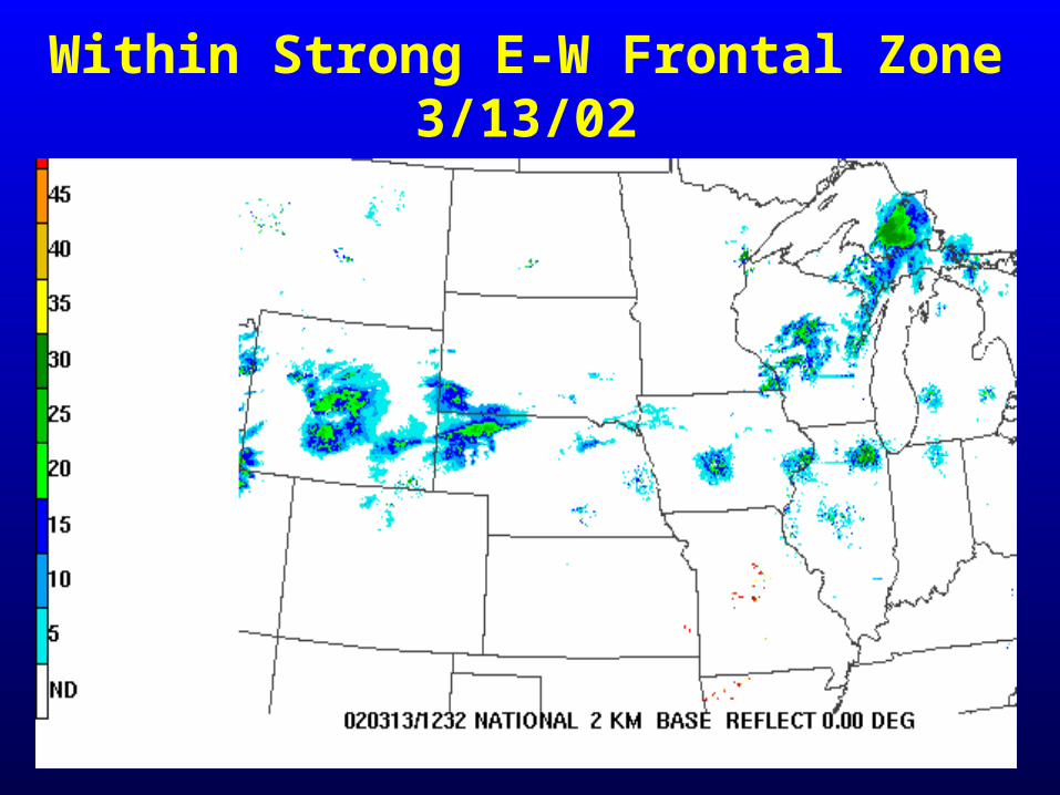
Within Strong E-W Frontal Zone3/13/02

Example Case of Frontogenesis and
Banded PrecipitationDate: 15 October 2001 (Case #1)
• Narrow band (1-2 counties wide) of moderate to heavy rainfall from eastern KS to central IL.
• Associated with weak surface features but a moderately strong baroclinic zone and frontogenesis forcing.
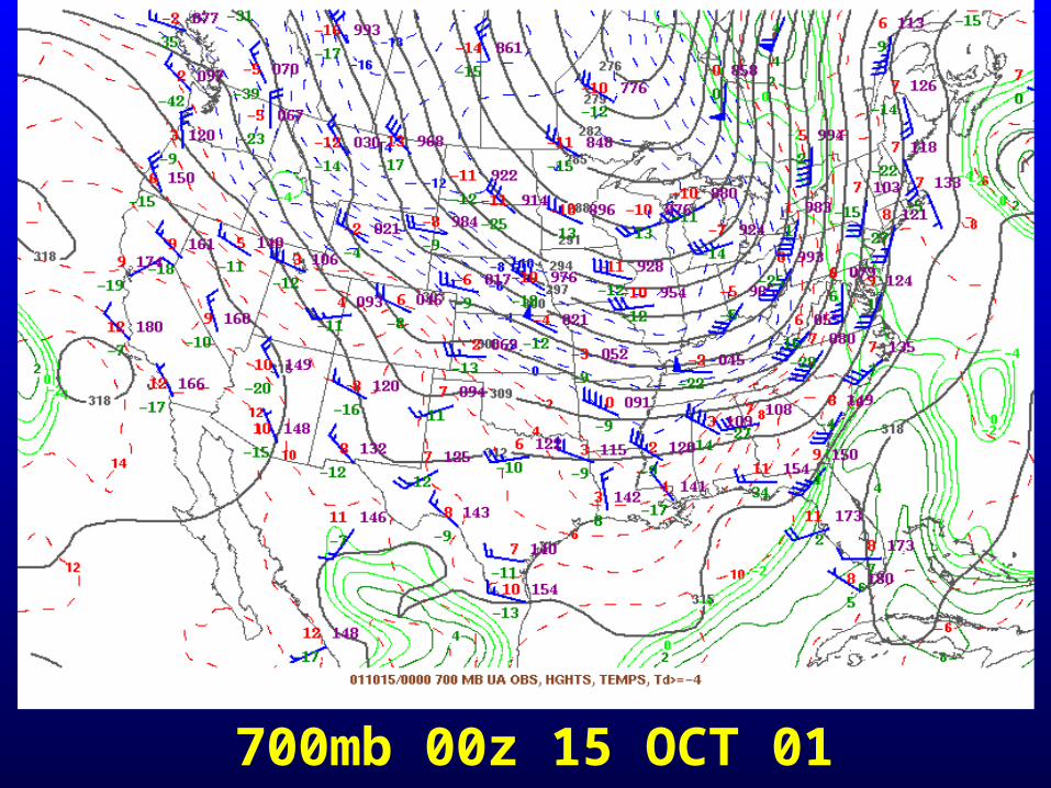
700mb 00z 15 OCT 01

Surface 15 OCT 2001
12z00z
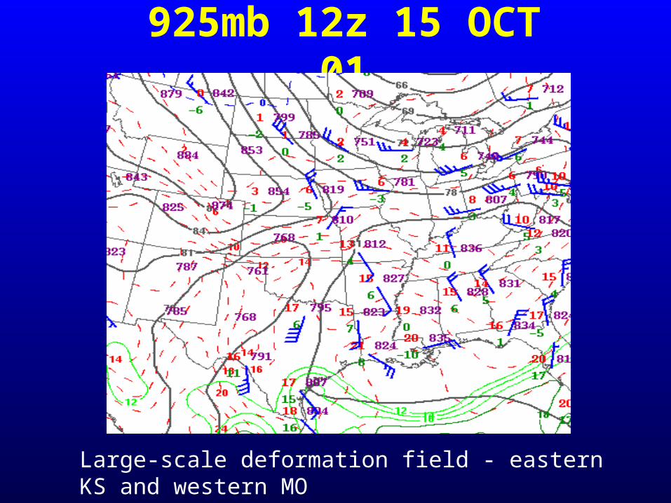
925mb 12z 15 OCT 01
Large-scale deformation field - eastern KS and western MO
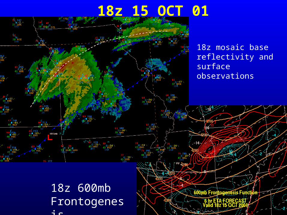
18z 15 OCT 01
18z 600mb Frontogenesis
18z mosaic base reflectivity and surface observations
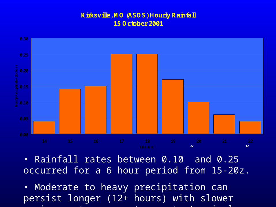
Kirksville, MO (ASOS) Hourly Rainfall15 October 2001
0.00
0.05
0.10
0.15
0.20
0.25
0.30
14 15 16 17 18 19 20 21 22TIME (UTC)
Ho
url
y P
rec
ipit
ati
on
(in
ch
es
)
• Rainfall rates between 0.10” and 0.25” occurred for a 6 hour period from 15-20z.
• Moderate to heavy precipitation can persist longer (12+ hours) with slower moving systems or mature extratropical cyclones.
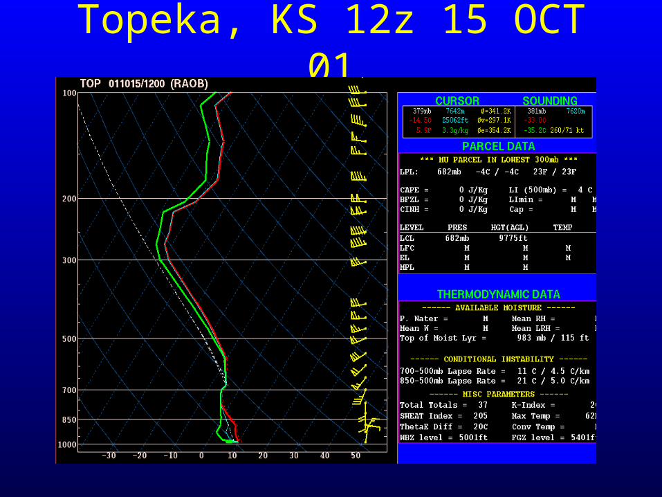
Topeka, KS 12z 15 OCT 01
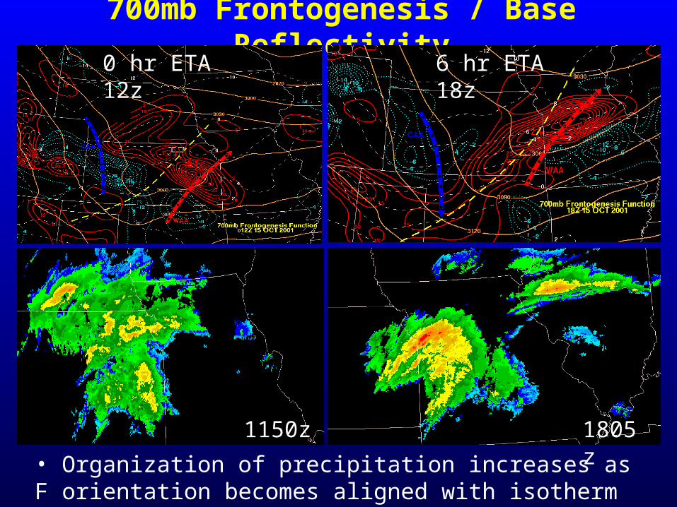
700mb Frontogenesis / Base Reflectivity
0 hr ETA 12z
6 hr ETA 18z
1150z 1805z • Organization of precipitation increases as F
orientation becomes aligned with isotherm orientation at lower levels.
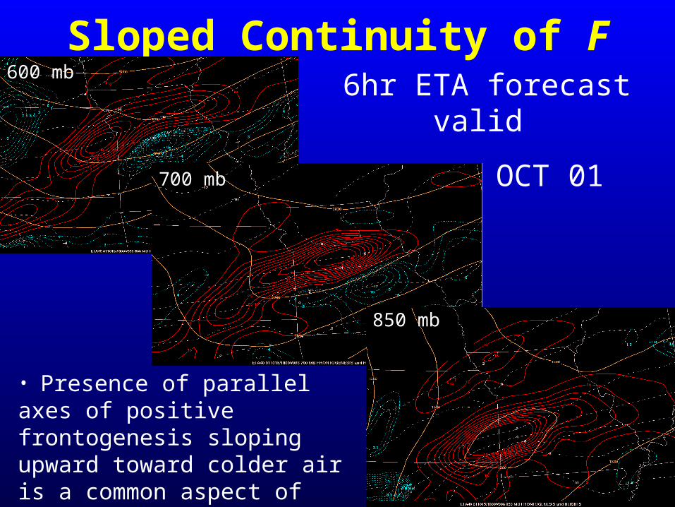
Sloped Continuity of F6hr ETA forecast
valid
18z 15 OCT 01
• Presence of parallel axes of positive frontogenesis sloping upward toward colder air is a common aspect of heavy banded precipitation areas.
600 mb
700 mb
850 mb

Sloped Continuity of F
The plane of the cross-section should be taken perpendicular to the mid-level (850-500mb) thermal wind vector or thickness lines.

Sloped Continuity of Frontogenesis Forcing
(cont.) The previous two slides have several important
implications:1) Several levels (or a x-section) should be assessed
for spatial continuity and orientation of F, to see if banding is likely to occur at a given time.
2) Vertical averaging should probably be avoided.3) The sloped continuity tells us something about the
structure of the wind field we can use to infer frontogenesis from single sounding (observed or model derived), VAD, or wind profiler data, and large-scale flow fields.
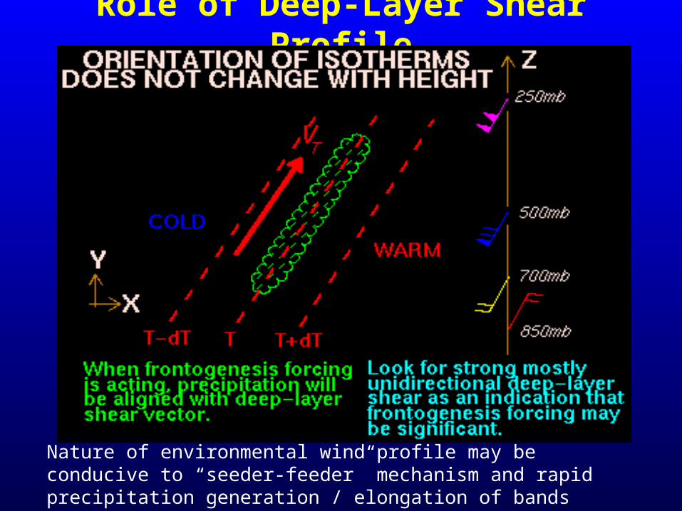
Role of Deep-Layer Shear Profile
Nature of environmental wind profile may be conducive to “seeder-feeder” mechanism and rapid precipitation generation / elongation of bands during initial development phase.
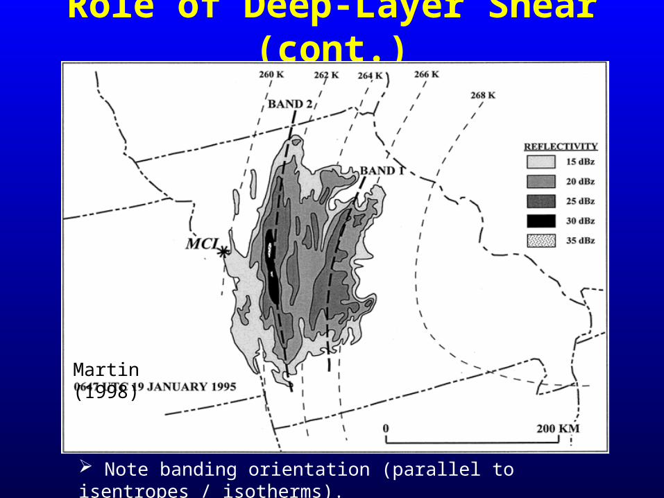
Role of Deep-Layer Shear (cont.)
Martin (1998)
Note banding orientation (parallel to isentropes / isotherms).
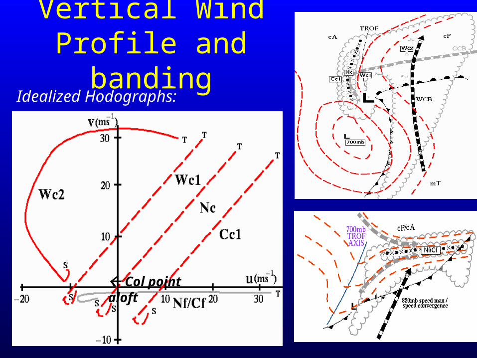
Vertical Wind Profile and
bandingIdealized Hodographs:
Col point aloft
Mesoscale Band Variations
- Band movement (short and long-axis translation)
- Warm season vs. cool season bands
- Multiple parallel bands (stability driven)
- Non-banded (the “null wind structure”)
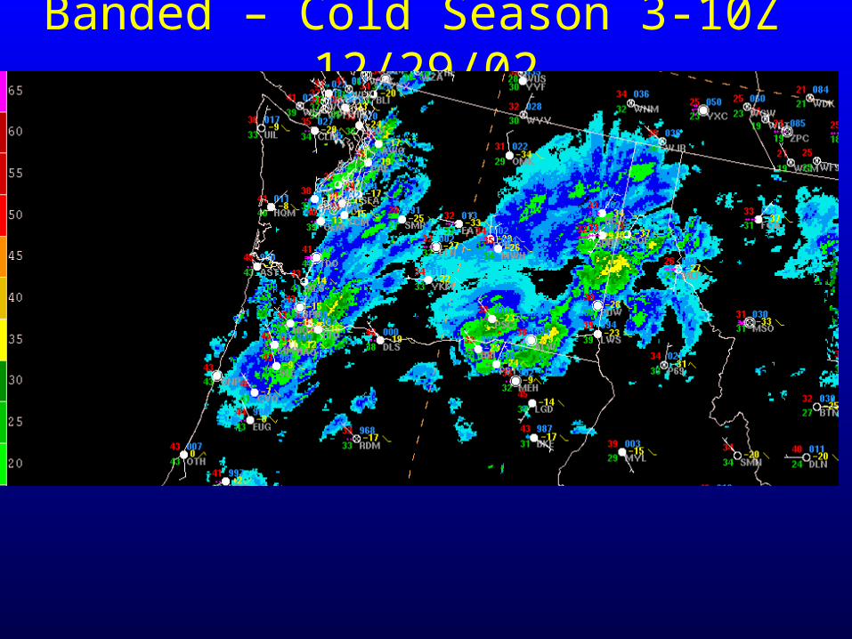
Banded – Cold Season 3-10Z 12/29/02
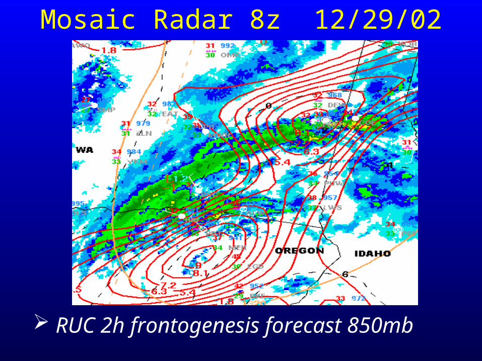
Mosaic Radar 8z 12/29/02
RUC 2h frontogenesis forecast 850mb
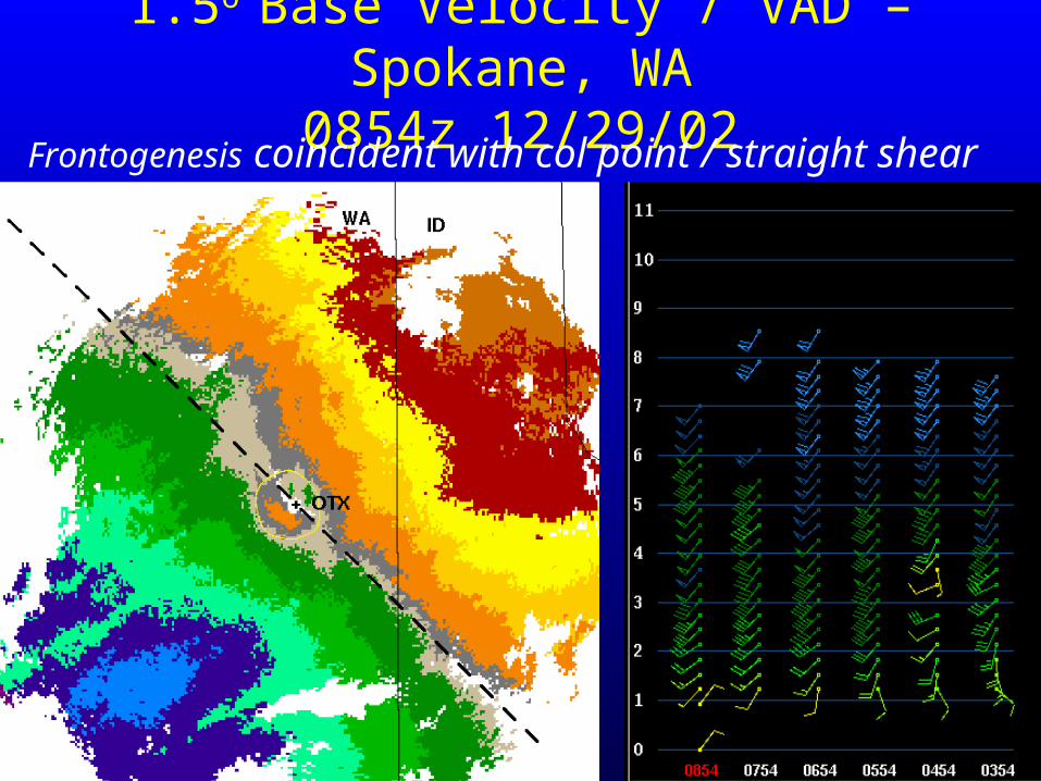
1.5o Base Velocity / VAD – Spokane, WA
0854z 12/29/02Frontogenesis coincident with col point / straight shear
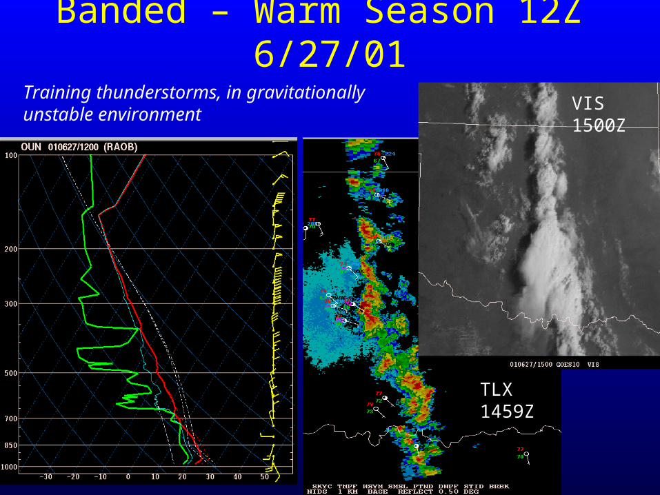
Banded – Warm Season 12Z 6/27/01
Training thunderstorms, in gravitationally unstable environment
TLX 1459Z
VIS 1500Z
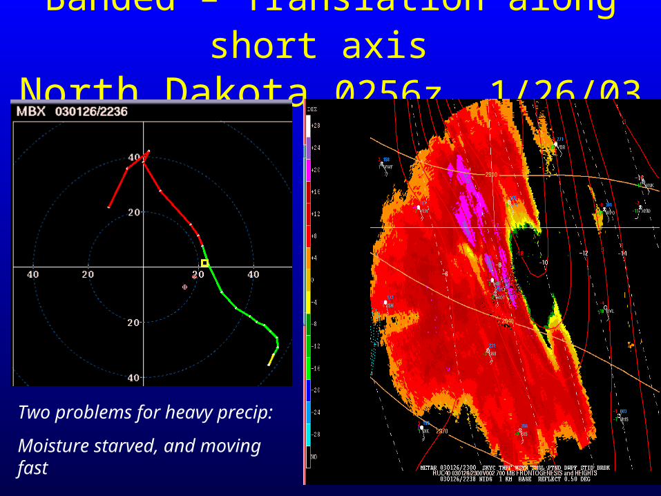
Banded – Translation along short axis
North Dakota 0256z 1/26/03
Two problems for heavy precip:
Moisture starved, and moving fast
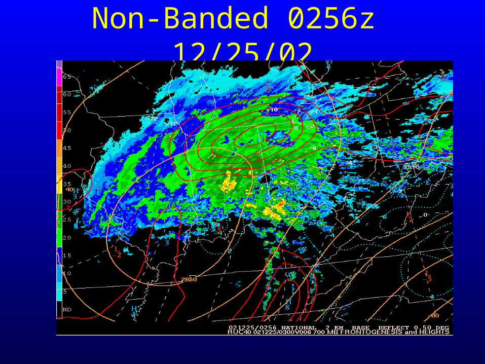
Non-Banded 0256z 12/25/02
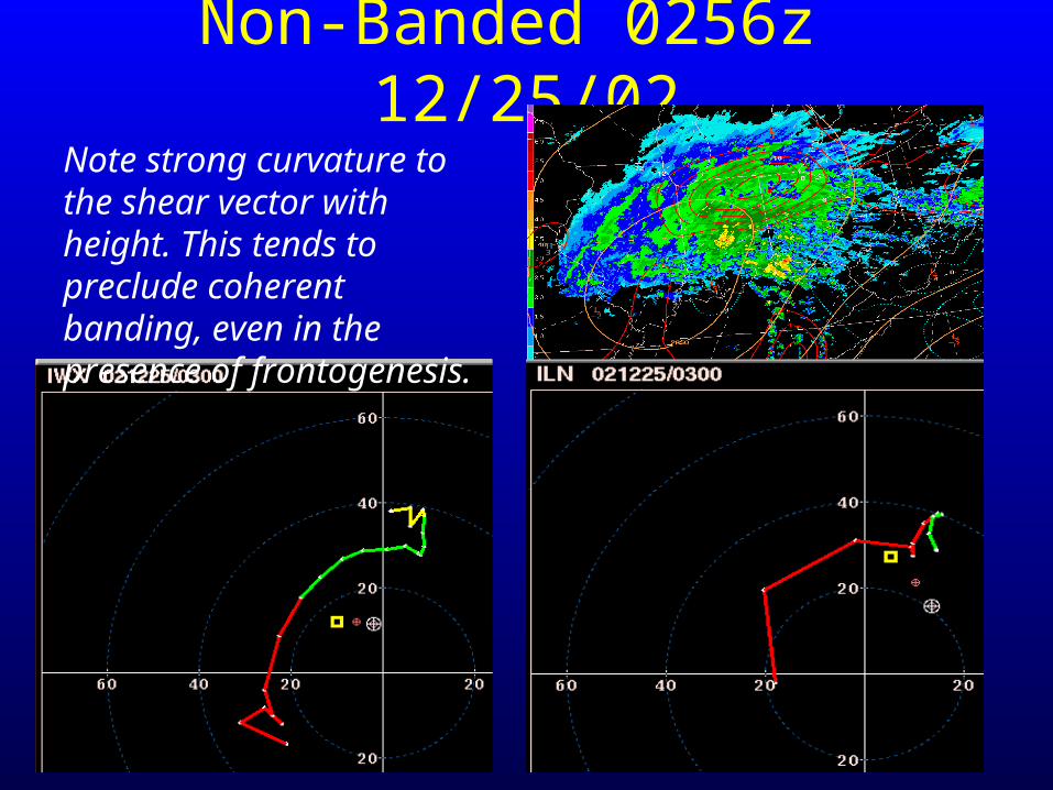
Non-Banded 0256z 12/25/02
Note strong curvature to the shear vector with height. This tends to preclude coherent banding, even in the presence of frontogenesis.
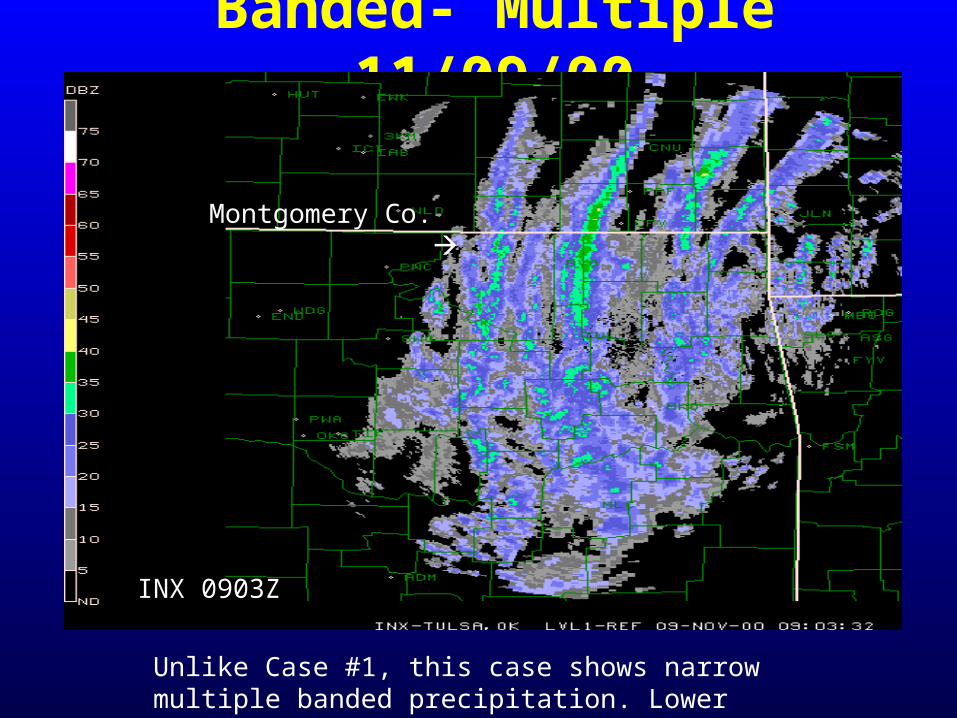
Banded- Multiple 11/09/00
INX 0903Z
Montgomery Co.
Unlike Case #1, this case shows narrow multiple banded precipitation. Lower stability likely played a role.
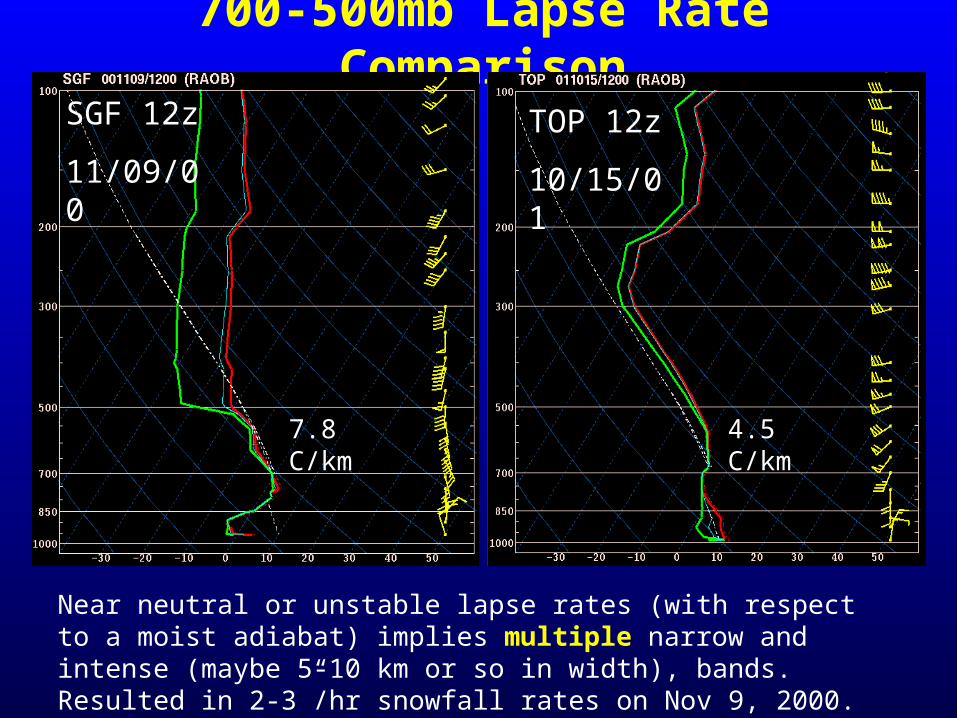
700-500mb Lapse Rate Comparison
Near neutral or unstable lapse rates (with respect to a moist adiabat) implies multiple narrow and intense (maybe 5-10 km or so in width), bands. Resulted in 2-3”/hr snowfall rates on Nov 9, 2000.
7.8 C/km
4.5 C/km
SGF 12z
11/09/00
TOP 12z
10/15/01
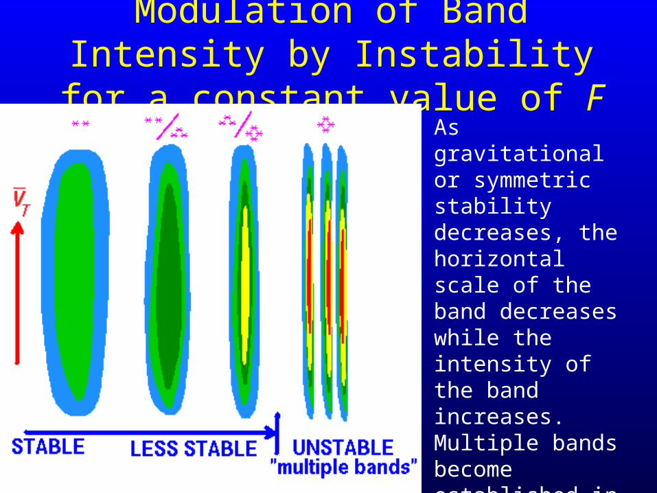
Modulation of Band Intensity by Instability for a constant value
of FAs gravitational or symmetric stability decreases, the horizontal scale of the band decreases while the intensity of the band increases. Multiple bands become established in an unstable regime.
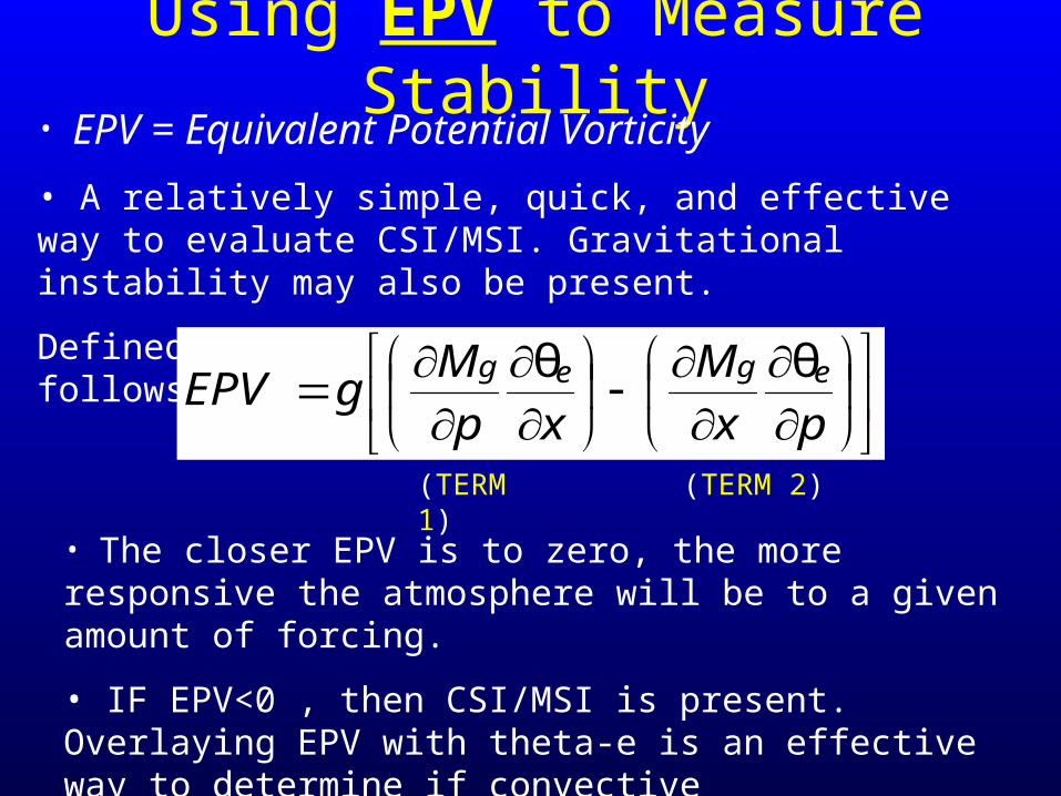
Using EPV to Measure Stability
• EPV = Equivalent Potential Vorticity
• A relatively simple, quick, and effective way to evaluate CSI/MSI. Gravitational instability may also be present.
Defined by Moore and Lambert (1993) as follows:
px
M
xp
MgEPV egeg θθ
(TERM 1) (TERM 2)
• The closer EPV is to zero, the more responsive the atmosphere will be to a given amount of forcing.
• IF EPV<0 , then CSI/MSI is present. Overlaying EPV with theta-e is an effective way to determine if convective (gravitational) instability also exists.
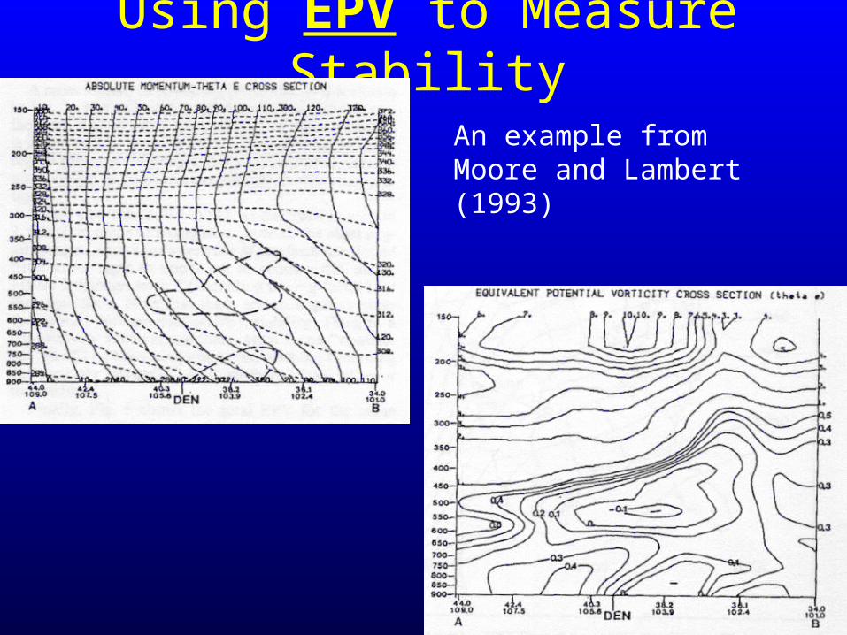
Using EPV to Measure Stability
An example from Moore and Lambert (1993)
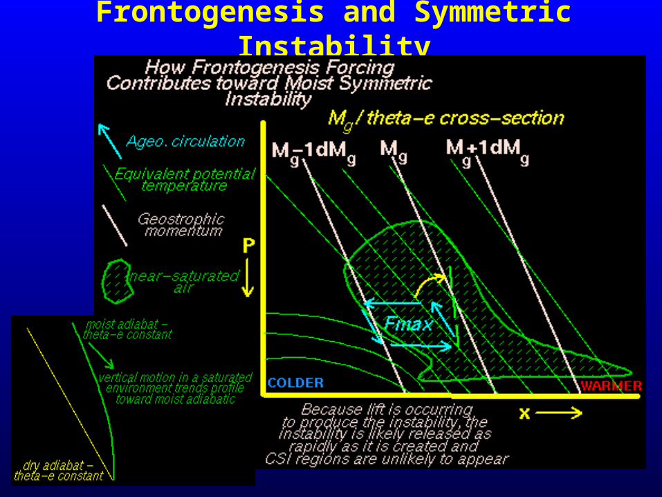
Frontogenesis and Symmetric Instability
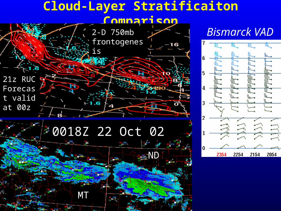
Cloud-Layer Stratificaiton Comparison
MT
ND
0018Z 22 Oct 02
21z RUC Forecast valid at 00z
2-D 750mb frontogenesis
Bismarck VAD
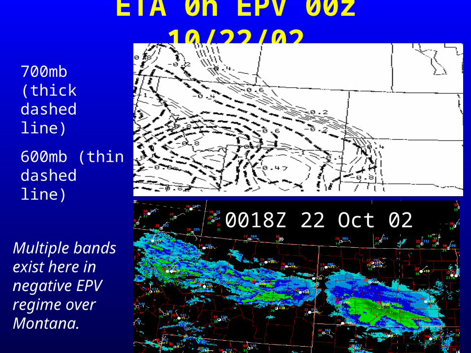
ETA 0h EPV 00z 10/22/02
0018Z 22 Oct 02
700mb (thick dashed line)
600mb (thin dashed line)
Multiple bands exist here in negative EPV regime over Montana.
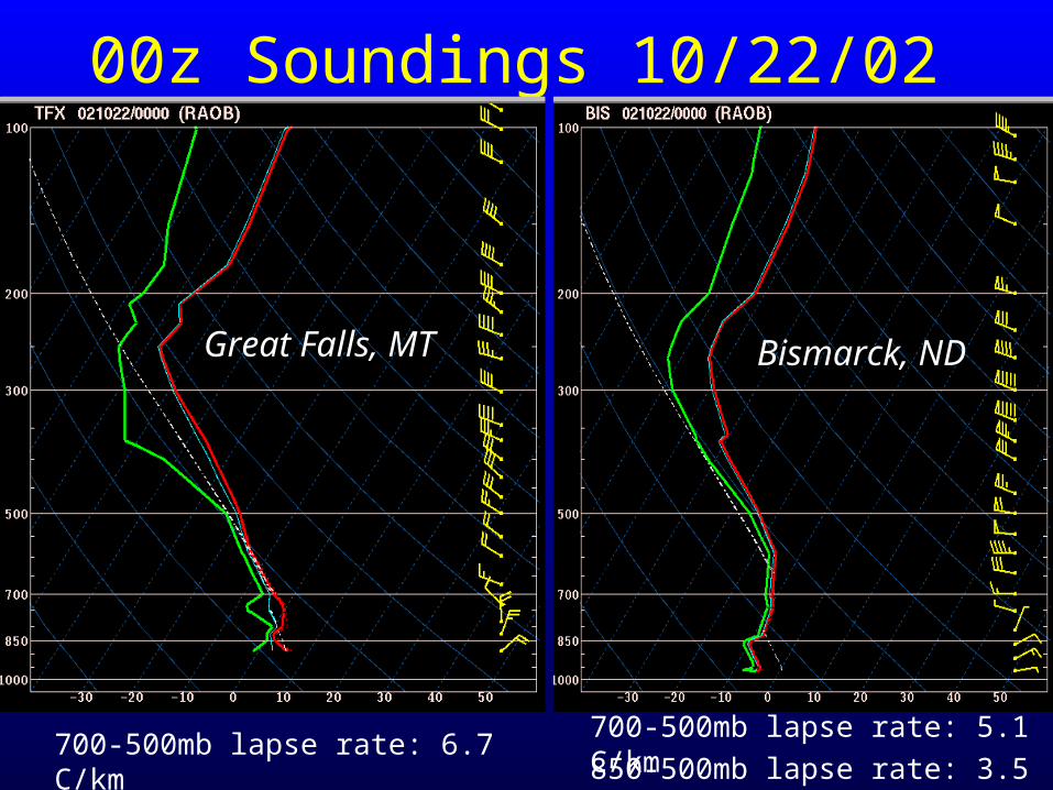
00z Soundings 10/22/02
850-500mb lapse rate: 3.5 C/km
700-500mb lapse rate: 6.7 C/km
700-500mb lapse rate: 5.1 C/km
Great Falls, MT
Bismarck, ND
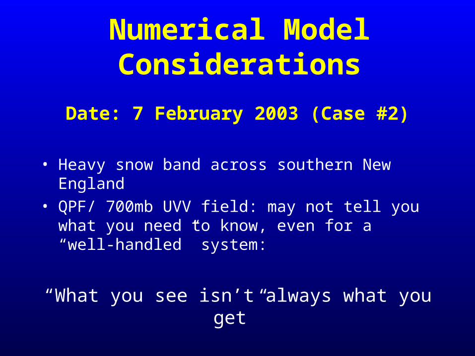
Numerical Model Considerations
Date: 7 February 2003 (Case #2)
• Heavy snow band across southern New England
• QPF/ 700mb UVV field: may not tell you what you need to know, even for a “well-handled” system:
“What you see isn’t always what you get”
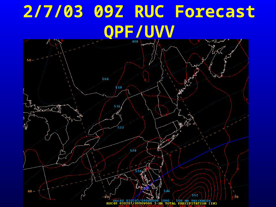
2/7/03 09Z RUC Forecast QPF/UVV
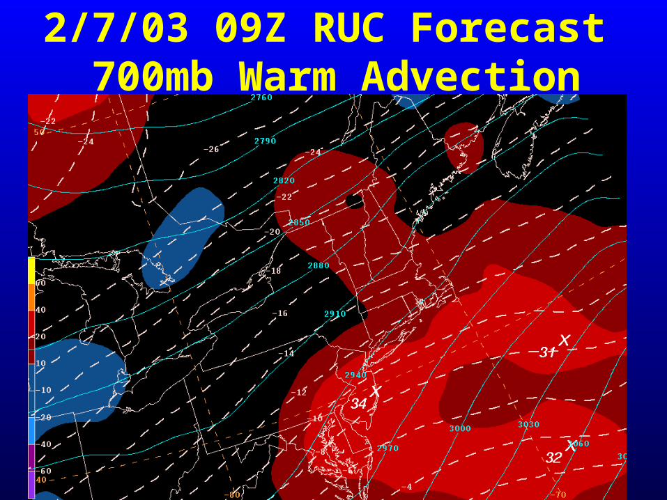
2/7/03 09Z RUC Forecast 700mb Warm Advection
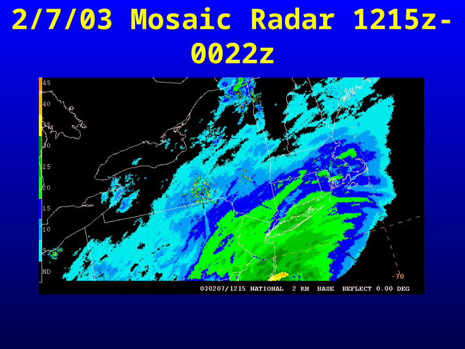
2/7/03 Mosaic Radar 1215z-0022z
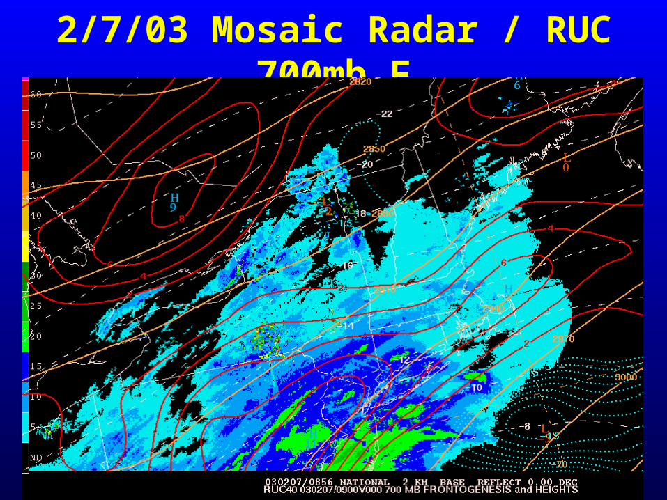
2/7/03 Mosaic Radar / RUC 700mb F
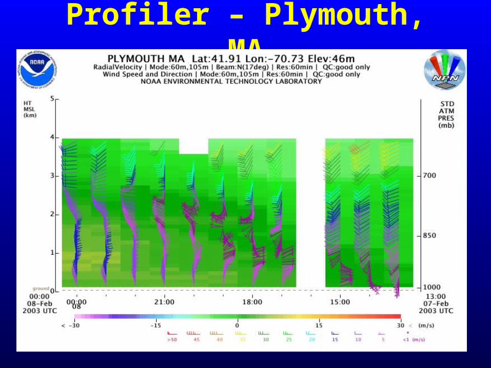
Profiler – Plymouth, MA

Boston, MA Surface Observations
BOS 13 UTC 1 1/2SM –SN
BOS 14 UTC 1/2 SM SN
BOS 15 UTC 1/2 SM SN SNINCR 1/ 2
BOS 16 UTC 1/2 SM SN SNINCR 1/ 3
BOS 17 UTC 1/2 SM SN SNINCR 2/ 4
BOS 18 UTC 1/4 SM +SN SNINCR 2/ 6
BOS 19 UTC 1/4 SM +SN SNINCR 2/ 8
BOS 20 UTC 1/4 SM +SN SNINCR 2/10
BOS 21 UTC 1/4 SM SN SNINCR 1/10
BOS 22 UTC 1/4 SM -SN
BOS 23 UTC 2 SM –SN
BOS 00 UTC 10 SM
700 mb
F, 18Z
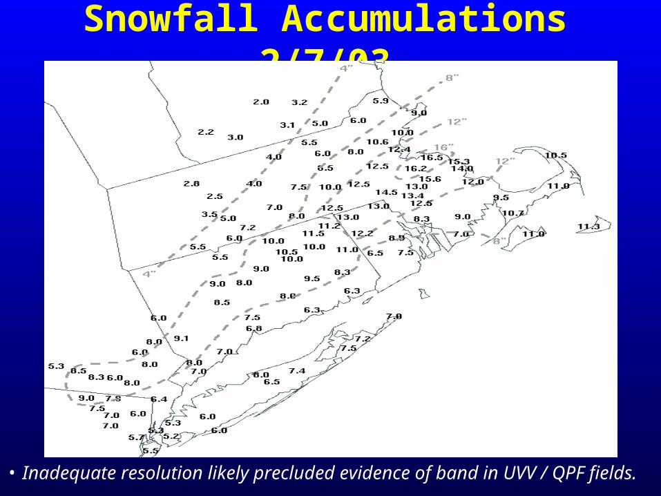
Snowfall Accumulations 2/7/03
• Inadequate resolution likely precluded evidence of band in UVV / QPF fields.

Suggested Snow Band Checklist
Presence of (1”/hr):
limited dry air advection in near surface.
near saturated / high low-mid level RH present (east CONUS, 1000-500mb >85%)
Favorable thermodynamic profile for snow (i.e. cloud top temp <-9C, no melting layers)
Sloped region of mid-level 2-D frontogenesis / Deformation axis in 850-500mb range
Relative minimum in wind speed (<20kt) within 850- 700mb region (col point aloft) and/or uniform deep- layer shear profile absence of substantial hodograph curvature
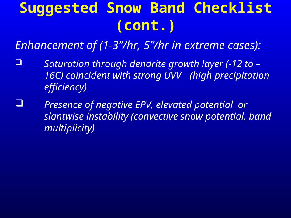
Suggested Snow Band Checklist (cont.)
Enhancement of (1-3”/hr, 5”/hr in extreme cases):
Saturation through dendrite growth layer (-12 to – 16C) coincident with strong UVV (high precipitation efficiency)
Presence of negative EPV, elevated potential or slantwise instability (convective snow potential, band multiplicity)
SUMMARY When applied within the context of ingredients based
forecasting, frontogenesis is useful for assessing potential for mesoscale banded precipitation areas.
Doesn’t require a strong cyclone, only a strong baroclinic zone, often developed through horizontal deformation and associated w/ a col point aloft
Col point aloft = YOUR cue to investigate F and banding potential
Location of col point aloft = approximate band location
Banding is modulated by wind structure and stability Banding is not always represented by the models