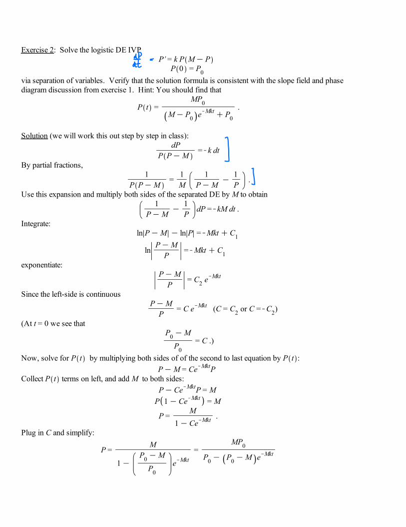
> >

Exercise 2: Solve the logistic DE IVPP = k P M P

P 0 = P0 via separation of variables. Verify that the solution formula is consistent with the slope field and phase diagram discussion from exercise 1. Hint: You should find that

P t =MP0

M P0 e Mkt P0

.

Solution (we will work this out step by step in class):dP

P P M= k dt

By partial fractions,1

P P M=

1M

1P M

1P

.

Use this expansion and multiply both sides of the separated DE by M to obtain1

P M1P

dP = kM dt .

Integrate:ln P M ln P = Mkt C1

lnP M

P= Mkt C1

exponentiate:P M

P= C2 e Mkt

Since the left-side is continuous

P M

P= C e Mkt (C = C2 or C = C2)

(At t = 0 we see thatP0 M

P0= C .)

Now, solve for P t by multiplying both sides of of the second to last equation by P t :P M = Ce MktP

Collect P t terms on left, and add M to both sides:P Ce MktP = M

P 1 Ce Mkt = M

P =M

1 Ce Mkt .

Plug in C and simplify:

P =M

1P0 M

P0e Mkt

=MP0

P0 P0 M e Mkt

P t =MP0

P0 M P0 e Mkt .

Finally, because limt

e Mkt = 0 , we see that

limt

P t =MP0

P0= M as expected.

Note: If P0 0 the denominator stays positive for t 0, so we know that the formula for P t is a differentiable function for all t 0. (If the denominator became zero, the function would blow up at the corresponding vertical asymptote.) To check that the denominator stays positive check that (i) if P0 M then the denominator is a sum of two positive terms; if P0 = M the separation algorithm actually fails because you divided by 0 to get started but the formula actually recovers the constant equilibrium solution P t M; and if P0 M then M P0 P0 so the second term in the denominator can never be negative enough to cancel out the positive P0 , for t 0 .)

P t =MP0

P0 M P0 e Mkt .

Finally, because limt

e Mkt = 0 , we see that

limt

P t =MP0

P0= M as expected.

Note: If P0 0 the denominator stays positive for t 0, so we know that the formula for P t is a differentiable function for all t 0. (If the denominator became zero, the function would blow up at the corresponding vertical asymptote.) To check that the denominator stays positive check that (i) if P0 M then the denominator is a sum of two positive terms; if P0 = M the separation algorithm actually fails because you divided by 0 to get started but the formula actually recovers the constant equilibrium solution P t M; and if P0 M then M P0 P0 so the second term in the denominator can never be negative enough to cancel out the positive P0 , for t 0 .)

Question: You have a couple of homework problems where you are asked to find solutions x t to differential equations of the form

x t = a x b x c .How would you proceed?

> >

> >

> >

> >

> >

> >

(1)(1)

(2)(2)> >

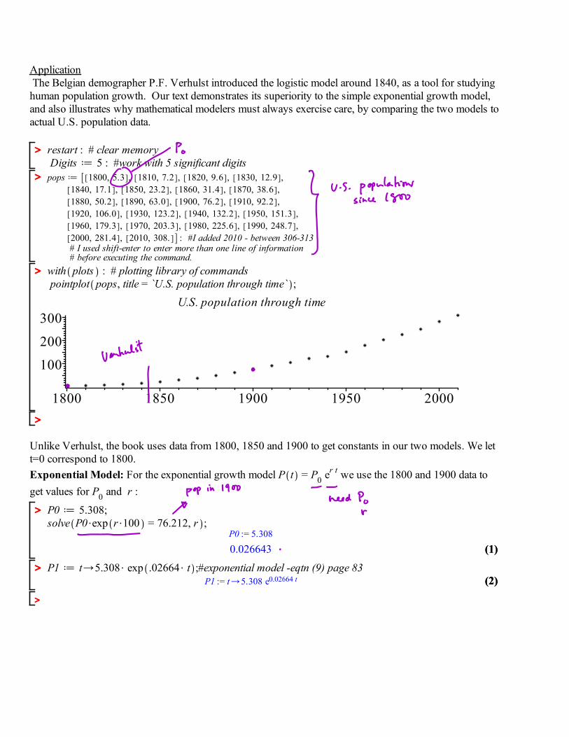
Application The Belgian demographer P.F. Verhulst introduced the logistic model around 1840, as a tool for studying human population growth. Our text demonstrates its superiority to the simple exponential growth model, and also illustrates why mathematical modelers must always exercise care, by comparing the two models toactual U.S. population data.

restart : # clear memory Digits 5 : #work with 5 significant digitspops 1800, 5.3 , 1810, 7.2 , 1820, 9.6 , 1830, 12.9 , 1840, 17.1 , 1850, 23.2 , 1860, 31.4 , 1870, 38.6 , 1880, 50.2 , 1890, 63.0 , 1900, 76.2 , 1910, 92.2 , 1920, 106.0 , 1930, 123.2 , 1940, 132.2 , 1950, 151.3 , 1960, 179.3 , 1970, 203.3 , 1980, 225.6 , 1990, 248.7 , 2000, 281.4 , 2010, 308. : #I added 2010 - between 306-313 # I used shift-enter to enter more than one line of information # before executing the command.with plots : # plotting library of commands pointplot pops, title = `U.S. population through time` ;

1800 1850 1900 1950 2000

100

200

300U.S. population through time

Unlike Verhulst, the book uses data from 1800, 1850 and 1900 to get constants in our two models. We let t=0 correspond to 1800. Exponential Model: For the exponential growth model P t = P0 er t we use the 1800 and 1900 data to get values for P0 and r :

P0 5.308;solve P0 exp r 100 = 76.212, r ;

P0 := 5.308

0.026643

P1 t 5.308 exp .02664 t ;#exponential model -eqtn (9) page 83P1 := t 5.308 e0.02664 t

> >

> >

(3)(3)

(5)(5)

> >

> >

(4)(4)

> >

> >

> >

Logistic Model: We get P0 from 1800, and use the 1850 and 1900 data to find k and M :

P2 t M P0 / P0 M P0 exp M k t ; # logistic solution we worked out

P2 := tM P0

P0 M P0 e M k t

solve P2 50 = 23.192, P2 100 = 76.212 , M, k ;M = 188.12, k = 0.00016772

M 188.12; k .16772e-3;P2 t ; #should be our logistic model function, #equation (11) page 84.

M := 188.12k := 0.00016772

998.545.308 182.81 e 0.031551 t

Now compare the two models with the real data, and discuss. The exponential model takes no account of the fact that the U.S. has only finite resources. Any ideas on why the logistic model begins to fail (with our parameters) around 1950?

plot1 plot P1 t 1800 , t = 1800 ..1950, color = black, linestyle = 3 : #this linestyle gives dashes for the exponential curveplot2 plot P2 t 1800 , t = 1800 ..2010, color = black :plot3 pointplot pops, symbol = cross :display plot1, plot2, plot3 , title = `U.S. population dataand models` ;

t1800 1850 1900 1950 2000

50100150200250300

U.S. population dataand models

Math 2280-01Wed Jan 282.2: Autonomous Differential Equations.

Recall, that a general first order DE for x = x t is written in standard form asx = f t, x ,

which is shorthand for x t = f t, x t . Definition: If the slope function f only depends on the value of x t , and not on t itself, then we call the first order differential equation autonomous:

x = f x .

Example: The logistic DE, P = k P M P is an autonomous differential equation for P t .

Definition: Constant solutions x t c to autonomous differential equations x = f x are calledequilibrium solutions. Since the derivative of a constant function x t c is zero, the values c of equilibrium solutions are exactly the roots c to f c = 0 .

Example: The functions P t 0 and P t M are the equilibrium solutions for the logistic DE.

Exercise 1: Find the equilibrium solutions of 1a) x t = 3 x x2

1b) x t = x3 2 x2 x

1c) x t = sin x .

Def: Let x t c be an equilibrium solution for an autonomous DE. Then · c is a stable equilibrium solution if solutions with initial values close enough to c stay close to c. There is a precise way to say this, but it requires quantifiers: For every 0 there exists a 0 so that for solutions with x 0 c , we have x t c for all t 0 . · c is an unstable equilibrium if it is not stable. · c is an asymptotically stable equilibrium solution if it's stable and in addition, if x 0 is close enough to c , then lim

tx t = c, i.e. there exists a 0 so that if x 0 c then

limt

x t = c . (Notice that this means the horizontal line x = c will be an asymptote to the solution graphs x = x t in these cases.)

Exercise 2: Use phase diagram analysis to guess the stability of the equilibrium solutions in Exercise 1. For (a) you've worked out a solution formula already, so you'll know you're right. For (b), (c), use the Theorem on the next page to justify your answers.

2a) x t = 3 x x2

2b) x t = x3 2 x2 x

2c) x t = sin x .

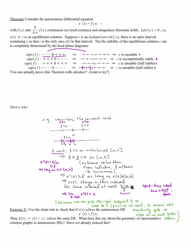
Theorem: Consider the autonomous differential equationx t = f x

with f x and x

f x continuous (so local existence and uniqueness theorems hold). Let f c = 0 , i.e.

x t c is an equilibrium solution. Suppose c is an isolated zero of f, i.e. there is an open interval containing c so that c is the only zero of f in that interval. The the stability of the equilibrium solution c canis completely determined by the local phase diagrams:

sign f : 0 c c is unstable sign f : 0 c c is asymptotically stable

sign f : 0 c c is unstable (half stable) sign f : 0 c c is unstable (half stable)

You can actually prove this Theorem with calculus!! (want to try?)

Here's why!

Exercise 3) Use the chain rule to check that if x t solves the autonomous DEx t = f x

Then X t x t c solves the same DE. What does this say about the geometry of representative solution graphs to autonomous DEs? Have we already noticed this?

Further application: Doomsday-extinction. With different hypotheses about fertility and mortality rates, one can arrive at a population model which looks like logistic, except the right hand side is the opposite of what it was in that case:

Logistic: P t = a P2 b P Doomsday-extinction: Q t = a Q2 b Q

For example, suppose that the chances of procreation are proportional to population density (think alligators or crickets), i.e. the fertility rate = a Q t , where Q t is the population at time t. Suppose themorbidity rate is constant, = b. With these assumptions the birth and death rates are a Q2 and b Q .... which yields the DE above. In this case factor the right side:

Q t = a Q Qba

= k Q Q M .

Exercise 4a) Construct the phase diagram for the general doomsday-extinction model and discuss the stability of the equilbrium solutions.