Organizational Behavior, Efficiency, and Dynamics in Non-ProfitMarkets: Evidence from Transitional Housing

James T. Edwards∗

December 1, 2013

Abstract

While there has been considerable research into patterns of charitable giving to non-profits, comparativelylittle is known about the behavior and motivations of organizations within these markets. This study forms adynamic model of oligopoly in a non-profit market, specifically allowing for organizational utility to followseveral specifications proposed by the literature: own revenues, own provision of services, and/or total marketsurplus. I obtain theoretical results on market efficiency under these different utility specifications, as well asfor different underlying market parameters. Using nationwide shelter-level panel data of U.S. transitional housingprograms, I employ the dynamic model to gain inference on the true specification of organizational utility. Finally,I use the estimated model to simulate market responses to shocks to the number of providers, the demand forservices, and the supply of contributions. None of the utility functions proposed by the literature significantlyexplains organizational behavior, with the results more consistent with a fixed organizational utility associatedwith entry. Relatedly, the market structure shows slow and relatively small responses to the simulated shocks.This questions the efficacy of increasing government donations to non-profits or the ability of non-profit marketsto increase production in response to a decrease in government service provision.

∗The University of Chicago, Department of Economics. I thank John List, Brent Hickman, Guenter Hitsch, Chad Syverson,Ronald Goettler, Rasool Zandvakil, Gregor Jarosch, Kevin Corinth, Leonardo Espinosa, and seminar participants at the University ofChicago for their helpful comments. I am also indebted to Rep. Charlie Dent, Dennis Culhane, and FOIA representatives at theDepartment of Housing and Urban Development for their help in data acquistion. Updated versions of the paper can be found athttp://home.uchicago.edu/˜jedwards/nonprofitbehavior.pdf.

1 IntroductionThe non-profit sector has a valuable role in the global economy, with the potential to correct various market

failures and provide a direct substitute for government provision of public goods. At the same time, there is a

concern that these institutions are shrouded from conventional competitive market forces, resulting in inefficiency,

ineptitude, and a lack of innovation in comparison to for-profit markets. At the extreme, the negative view of non-

profits holds that these organizations are simply “for-profits in disguise”, employing their non-profit status solely

to attain higher levels of net revenue, and circumventing monetary non-distribution constraints by transferring rents

through employee salaries and other benefits.

Understanding the relative performance of the non-profit sector in terms of efficiency and welfare, as well as the

policy that can be employed to increase these measures, is an issue that comes with increasingly high stakes. In

2010, non-profit organizations in the United States reported total revenues of $1.51 trillion, or 9.6% of GDP (The

Non-Profit Almanac, 2012). This is a figure that has risen steadily over the past thirty years. In an age of increasing

global fiscal austerity, non-profits in many fields have and will be asked to do more in response to the reduction in

government services. The ability of non-profits markets to respond to changing market conditions and the increase

in demand for their services is an important welfare concern. At the same time, governments often exist as the

major donor in many non-profit markets. This calls into question how efficiently public funds are being spent,

and whether the market power afforded by the status of lead contributor can be wielded to create superior market

outcomes.

Analyzing the expected market outcomes of the non-profit sector requires a two-fold approach. The most primal

concern is quantifying what actually motivates the managers of the organizations within the sector, thus defining the

actions that lead to market equilibria and dynamics. Just as important, however, is the analysis of the constraints

faced by these organizations. Specific market conditions, particularly the behavior of donors, have great power to

affect observed outcomes, regardless of the objective function of the organizations themselves.

The literature on non-profits has failed to adequately address either of these issues. There are several distinct

theories behind the motivation of non-profit entrepreneurs and organizations. The major specifications of non-profit

objective functions put forth by the literature are that these organizations maximize their own output, total market

surplus, or their net-revenue. Parsing between these theories becomes an empirical question, and there have been

several empirical studies attempting to answer it. This work has several unifying characteristics. Firstly, it has

almost exclusively been limited to the health care sector, presumably due to the prevalence of data and interest

in health care outcomes. Due to the nature of this sector, the empirical strategy employed by researchers has

been to attempt to confirm testable predictions of differential behavior between non-profits and for-profits. This

approach has failed to provide conclusive identification of the true motivation of non-profits, with research leading

to conflicting results, and a question of whether endogenous differences between the market realities faced by non-

profit and for-profits have been adequately controlled for. As noted in Horowitz and Nichols (2007), the lack of

clear inference may result from the difficulty of estimating or even generating conclusive predictions in an industry

rife with well known market failures.

Limiting research on organizational behavior solely to the health care field has an additional drawback of fo-

cusing on a sub-sector that is in many ways not representative of non-profit organizations as a whole. Non-profit

hospitals represent a very distinct subset of non-profits, notably one that receives almost all of its income from com-

mercial enterprise. One of the defining characteristics of many non-profit markets is that the vast majority of revenue

1

is received from charitable donations rather than the sale of goods. Empirical and theoretical research focusing on

non-profit markets where donations are a large portion of revenue tend to focus solely on the fundraising process

itself. This literature often appears to subscribe to an implicit belief that the welfare gain resulting from a specific

market is completely defined by the amount of donation money entering the market. What is more, the response of

donors to the structure of markets, such as the amount of additional marketwide donations resulting from an addi-

tional entrant, is poorly understood. Only recently have researchers diverged from a “manna from heaven” view of

donation and allowed organizations an active role in resource accrual. There has been less interest, however, on the

active role of these organizations in other decisions such as entry, exit, and investment in these markets.

Even leaving aside the lack of conclusive inference on the nature of organizational behavior, the empirical

literature has failed to answer how this behavior affects the performance of non-profit markets in terms of efficient

production of public goods and in response to shocks in market structure. No matter the true specification of

organization’s objective functions, the magnitude to which these motivations affect practical market outcomes is

unanswered. The reduced form focus on individual organizations rather than markets as a whole has left unclear the

efficacy of policy levers such as increasing donations to non-profits and reducing active government participation in

these markets. It is even unclear how these markets will respond to changes in societal demand for their services.

This work seeks to fill this void in the literature in several ways. First, I build a simple entry-exit model of

oligopoly in a non-profit market where contributions make up a substantial portion of organizational income. I

derive a variety of theoretical results within this model for several specifications of the objective function being

maximized by non-profits. This analysis centers primarily on the relative optimality of free entry of non-profit

organizations as a function of these objective functions under different market conditions. I find that not only

do different organizational objective functions lead to different predictions in the optimality of free entry and the

response to market shocks, but that free entry should not be expected to lead to socially optimal outcomes regardless

of the true objective function specification.

With this theory as a backdrop, I modify the model into a dynamic empirical framework in the spirit of Ericson

and Pakes (1995). From several data sources, I form a rich dataset of the U.S. transitional housing sector that

includes data on individual shelter capacities, market demand shares, donation revenues, and assets. The data

also include market level data on the number of homeless individuals in each jurisdiction, and have the advantage

of displaying naturally delineated regional markets, completeness in terms of entered organizations, and an easily

quantifiable good in the amount of beds provided. I employ observed organizational behavior in entry, exit, and

capacity to reveal which of the proposed objective specifications best describe organizations actions.

My empirical strategy, a modification of the estimator of Bajari, Benkard and Levin (2007), forward simulates

the structural model to determine the expected utility resulting from an action that the organization does take, as

well as actions that they did not. I then estimate utility parameters under each of the proposed objective function

specifications by finding the values that maximize the likelihood of observed actions given the relative expected

utilities. This allows me to determine how well each proposed specification fits the data. The forward simulation

is made tractable by a reduction of a large state space into a smaller set of market moments that affect future

organizational utility, and a structural vector autoregressive (sVAR) process that governs the transition of these

moments and allows them to be conditional on individual organization actions. The sVAR structure also allows me

to simulate market responses to both short-term and long-term shocks to market conditions. I employ this to estimate

market responses to shocks in the demand for services, shocks in donations to the market, and supply shocks which

2

simulate a reduction in direct government services in the market.

I find several interesting results. Most importantly, I find that the non-profit sector in question does not respond

rapidly or strongly to changes in market structure resulting from the above shocks. A 25% long-term increase

in demanders only results in a estimated 10% increase in market capacity over a 10 year period. A 25% one

period increase in market donations has no discernable effect on capacity. Finally, a 25% drop in market supply

capacity only results in an increase to 85% of the original market capacity in a 10 year period. Next, there is little

evidence supporting the own provision maximization, market surplus maximization, and net-revenue maximization

specifications of organizational utility espoused by the literature. This assertion is supported by reduced form

analysis of organization’s policy functions. The data instead supports the idea that practitioners of non-profits

receive fixed or idiosyncratic utility not highly correlated with these simple market values.

The first-stage estimation of a end consumer demand system with capacity constrained options and a donation

system leads to additional insights. Most notably, I find no evidence that the presence of additional organizations in

a market leads to additional total market donation to that market.

Section 2 discusses the relationship of this paper with the existing literature on non-profits. In Section 3, I build

a simple theoretical model of non-profit oligopoly with contributions as the major source of income. Sections 4

summarizes the transitional housing sector and describe the data. Sections 5 and 6 specify the dynamic empirical

model and my empirical strategy. Section 7 presents my empirical results, and Section 8 presents the simulations of

market shocks. Section 9 discusses the results as a whole, and Section 10 concludes.

2 Relationship to Existing LiteratureThree major specifications of the objective function maximized by non-profit firms have been suggested in

the literature. The first, originally put forth by Newman (1970), posits that non-profits are output-maximizers,

subject to some financial constraint that insures they remain solvent. The general justification of this specification

is that non-profit organizations either attract or are founded by individuals who care about provision of the good

produced by the organization (Rose-Ackerman 1996). Importantly, this output-maximization only encompasses

an organization’s own provision of services, and not the total production of the public good. Under this objective

function, an organization would receive return from providing goods in a market, even if counter-factually the same

level of goods would be provided if the organization was not active in the market. The root of this desire for own

provision of the good can be modeled similarly to that of donors to public goods: a justification of this objective

function is that the managers of non-profits are not truly altruistic, but rather receive warm-glow utility from being

the direct provider of services (see Andreoni 1990 for a discussion of warm-glow). Alternatively, if the organization

managers are direct consumers of the good in question (consider for example non-profit arts programs, see Ben-Ner

1983) they may enjoy privileged consumption or perceived ability to affect the characteristics of the good should

they produce it.

Organizations may alternatively have an objective function that maximizes market output or market surplus

(Weisbrod 1988). This surplus is traditionally viewed as the surplus resulting from consumption of the good pro-

duced by the market. In this view, organizations will in fact take into account their marginal effect in the market,

and on total output or surplus. A theoretical justification of this theory is similar to that above, however in this case,

non-profits managers are either truly altruistic, or consume the good in a way that is unaffected by the identity of its

producer.

3

Finally, on the other side of the spectrum is the view that non-profits are in fact actually profit maximizers.

This for-profit in disguise specification was first described by Pauly and Redisch (1973) which modeled non-profit

hospitals simply as physician collectives which reaped market rents as higher wage levels. Although returning net-

revenue to employees is obviously forbidden by the non-distribution constraint (Hansmann 1980) required of non-

profits, it is conceivable that this sort of transfer still occurs implicitly through wage contracts, laxity regarding the

enforcement of rules for non-profits, and symbiotic cooperation between non-profit employees and board members.

Several other strains of theory regarding the objective function are also extant. These include various theories

combining two of the above three specifications, the maximization of perquisites other than output related to man-

aging a non-profit, and other motivations of organizational creation generic to entrepreneurs (see Steinberg 2006 for

a longer discussion).

Empirical research attempting to parse between these theories has been inconclusive and contained almost en-

tirely within the health-care sector. The usual empirical strategy of these works is to attempt to confirm some

theoretically proven differential in behavior between non-profit and for-profit hospitals. Sloan and Vraciu (1983)

find no observable differences in the provision or pricing of services between the two types of producers, while other

studies conclude that non-profits provide better quality care (Shen, 2002) or a higher proportion of unprofitable care

(Horowitz 2005, Schlesinger et. al 1997), suggesting motives other than profit-maximization. Chang and Jacobson

(2012) and Deneffe and Mason (2002) reject models of pure profit maximization or pure surplus maximization, and

Horowitz and Nichols (2007) support some mixture of quality and output provision as entering the utility function.

These studies are hampered, however, by the attempt to find true exogenous variation in a market as complicated in

structure as that of health care.

Research on other non-profit sectors typically focuses on giving patterns of donors. There is a large literature on

how charitable giving is affected by tax rates, notably Clotfelter (1985), Randolph (1995), and Auten et. al (2002).

Another well-researched topic is on how government spending crowds out private giving, e.g. Payne (1998) and

Okten and Weisbrod (2000). These papers typically assume a static role of organizations in the fundraising process,

an idea that was corrected by Andreoni and Payne (2003), who allowed organizations active decisions in the extent of

effort put forth in fundraising. They found that crowd out of private giving in response to government giving could

be explained significantly by lower expenditures on fundraising by organizations once they had received government

grants.

The only paper to my knowledge outside of the health care sector that specifically looks at non-profit output

decisions is Hungerman (2005), who looks at the spending response of Presbyterian denomination churches to

changes in government spending on human services resulting from the 1996 welfare reform. He finds a significant

response in terms of church spending on human services in response to the shock.

Another literature important in relationship to this work is the question of the value of non-profits in a general

equilibrium sense. The prevailing explanation of why non-profits exist and their value to society is the “three

failures theory” first posited by Weisbrod (1975) and developed by Hansmann (1980) and Salamon (1987). In

this theory, non-profits respond to market failure and government failure to provide adequate levels of a public

good that is valued by society. Market failure can result from allocative inefficiencies, free-rider problems, or

contract failure. Although governments on some level can fill this underprovision in public goods, political economy

interactions may lead to a level still too low or misallocated in relation to the desire of some citizens. Non-profits

thus exist to complement and augment this government provision of services. The third failure is within non-

4

profits themselves: non-profits can still be unable to provide an adequate level of services due to philanthropic

insufficiency, particularism, paternalism, and amateurism (again, see Steinberg 2006 for a longer discussion of this

theory). Important in relation to the empirical results of this paper are particularism, where non-profits focus on

specific groups at the expense of others, paternalism, where the practitioners of organizations address problems as

they see them rather then as society values them, and amateurism, where non-profits employ workers with inadequate

skills to capably address the underprovision of the good in question. These are discussed in relation to the empirical

results at the end of the paper.

3 ModelThe first task in modeling a non-profit is defining the scope of that market. Unlike in for-profits, where the set

of firms constituting the market is defined by the substitutability of the goods they provide to consumers, non-profits

can compete not only in the provision of goods, but also in the acquisition of donations. While the degree of good

competition for non-profits is expected to vary in each market similarly to for-profit markets, the lack of knowledge

of donor behavior makes the extent of competition between firms in donation acquisition an open question. Donor

pools may at one extreme be completely disjoint for different firms, resulting in no competition for donations. At the

other extreme, firms may be actively competing for each donation dollar with every other extant firm, regardless of

product or region. My own discussions with non-profit practitioners indicate that they unanimously feel competition

from other firms when securing funding, and that this competition primarily comes from firms providing similar

goods and services in their region. As such, the model, while general, is geared to oligopolistic markets where firms

experience some degree of competition both on the end consumer and donor markets.

To model a non-profit market, I separate the agents into three groups: end consumers, donors, and non-profit

firms. Let there be i = 1, ...I donors, j = 1, ..., J end consumers, and n = 1, ..., N entered firms in the market1.

End Consumers End consumers are the population of individuals to whom the good provided by the market is

available. These individuals pay (a possibly zero price) for the good, may incur costs of consumption beyond the

price of the good, and may overlap with donors. The consumption choice of end consumers is modeled in a discrete

choice framework between the firms in the market and an outside option. I further assume that each end consumer

can only consume a single unit of the good. The indirect utility of end consumer j of consuming from firm n is

given as:

Vjn = fECj (Xn) + V n + ejn

where Xn is a k-dimensional vector of firm characteristics, fCj is an unspecified function, V n is the average

idiosyncratic taste variable associated with firm n (shared for all individuals), and ejn is a stochastic term from an

unspecified mean-zero distribution. The utility of the outside no consumption option V0n is normalized to 0. End

consumers consume one unit of the option with the highest Vjn.

Donors Donors constitute any individual or group that could possibly donate money to a firm in the non-profit

market. This encompasses private individuals, public foundations, corporations, and the government. The role of

donors is to choose which (if any) firm to give to, and if so, how much to give. The donation choice of donors is

modeled in a discrete choice framework similar to that of end consumers. The indirect utility of potential donor i1I will refer to non-profit organizations as firms for the remainder of the paper to keep with the standard of industrial organization models.

5

associated with giving to firm n be given as:

Win = fDi (Xn) +Wn + uin

where Xn is a k-dimensional vector of firm characteristics, fDi is an unspecified function, Wn is the average

idiosyncratic taste variable associated with firm n (shared for all individuals), and uin is a stochastic term from an

unspecified mean-zero distribution. The utility of the outside no donation option W0n is normalized to 0. Potential

donors donate an amount δ(Win) to its highest utility option. I assume ∂δ(Win)∂Win

≥ 0, that is, the higher the utility of

donation, the weakly higher the amount donated.

Non-Profit Firms The firms choose whether to enter the market, when to exit, and in some cases make decisions

on other choice variables such as the quantity supplied, prices, capacity investments, and fundraising intensity.

Each firm has an unspecified utility function U(.), and has outside utility Yn > 0 which they receive if they are

not in the market. Firms are also defined by a cost function Cn(Q) and their characteristics Xn2.

Of prime importance in characterizing the equilibrium in this market is the specification of the firm utility

function. As discussed above there are three major potential motivations suggested by the literature to dictate the

decisions of non-profits. For the sake of this analysis, I have limited the terms entering firm’s utility functions to

these three possibilities:

1. Own Provision: Firms maximize their own provision of goods min(Qn, Dn), where Qn is the amount of the

good supplied by the firm and Dn is end consumer demand for their good.

2. Market Surplus: Firms maximize end consumer market surplus CSm.

3. Net Revenue: Firms receive utility from net revenue Rn−Cn(Qn). This monetary return is primarily passed

to firm members through higher salaries or benefits.

3.1 One-Period Model

Many of the important mechanics that lead to market equilibria can be illustrated in a simple one period model.

Here I discuss the results of the model integral to my empirical work, with a more formal discussion given in

Appendix A. Let there be M potentially entering firms and unit measures of end consumers and donors. For

simplicity, I initially assume symmetric firms, no scope for fundraising, no ability to price goods above zero, and

“oblivious” donors and end consumers with Vjn = V + ejn,∀j and Win = W + uin ,∀i 3 .

Under the very weak assumption that the stochastic utility error terms for end consumers eimand donors ujm are

drawn from unspecified donations with non-perfectly correlated draws and full supports, total market donations and

total market end consumer demand increases with the entry of a new firm. Intuitively, this results from a taste for

variety on the part of donors and end consumers. Total market donations and total market end demand for the good

increase concavely with the number of entrants, however, resulting in mean firm donations and mean firm demand

decreasing in the number of entrants. An additional entrant thus leads to both market expansion and “stealing” from

other incumbents in the donation and end demand markets.2 These characteristics can include product characteristics and taste characteristics, and potentially enter donor or patron utility above.

Due to their generic nature, these characteristics can be modeled as exogenous or chosen by the firm.3This is a stronger condition than saying the firms are symmetric, as it limits donors from having variation in taste based on equilibrium

values such as service provision, marginal surplus, and efficiency of the firms.

6

Firms face two constraints on their ability to provide goods to end consumers: they must have end demand Dn

for the amount of goods Qn they supply, and they must have revenue Rn =∑iδin to pay for the cost of production

of Qn. Even if firms are Net Revenue maximizers, and are not seeking to maximize own or market output, revenues

Rn associated with entry will obviously affect their return of being in the market. Thus, in each specification either

the end demand or donation markets define the entry behavior of firms.

Equilibrium entry patterns are defined by the number of entrants such that the return of entry is equal to firm’s

outside option Y (assuming entrants and non-entrants, and ignoring integer constraints). Under the three specifica-

tions, this leads to the number of entrants NFE that solves:

Own Provision : min(C−1(R(N)), D(N)) = Y

Market Surplus : CS(N)− CS(N − 1) = Y

Net Revenue : R(N)− C(0) = Y

Note that under this simple set up, Net Revenue maximizers will choose not produce any goods and must only pay

a fixed cost of production. This has the potential to change as the assumption of “oblivious” donors is dropped, as

discussed below.

3.1.1 Efficiency of Free Entry

How does free entry in the above specifications compare to socially optimal entry? First, one must define

what a social planner should optimize. For the remainder of the paper, I will treat the surplus of the market as

being the surplus of the end consumers of the good. This falls into the “three failures theory” discussed above,

in that the societal value of the market is its added provision of a good that is underallocated due to market and

government failures. One might also wish to include in market surplus donor utility and firm utility to the extent

that it differs from consumer surplus. My justification for limiting the discussion of surplus to end consumers is that

the differences between these marginal surpluses and the marginal surplus of end consumers is likely second order,

and focusing only on end consumer surplus allows for more exact predictions in terms of the optimality of different

market structures.

A social planner limited to the second-best choice of the number of entrants will choose the number of entrants

N∗ that maximizes end consumer surplus:

CS(N) = N min(C−1(R(N)), D(N))EUEC(N)

where EUEC , the expected end consumer utility of consuming a unit of the good, is concavely increasing in N .

Note that an additional entrant can never decrease end consumer surplus as long as C−1(R(N)) > D(N), or the

amount of good that can be produced by each firm based on their revenue is higher than end consumer demand for

each firm. In this case an extra entrant will increase market demand, and this demand will be able to be fulfilled

by supply, raising surplus. Thus the constraint that must hold is the revenue constraint, resulting in the first order

condition:

(C−1(R(N)) +N∂C−1

∂R

∂R

∂N)EUEC(N) +NC−1(R(N))

∂EUEC(N)

∂N= 0

The second term in this equation denotes the increase in surplus due to the taste for variety by end consumers,

7

and will always be positive. The first denotes the change in good production resulting from the redistribution of

donations due to entry: the overall amount of market donations increases, but each individual firm receives less

revenue. This will be surplus reducing if the possibly negative effect of the change in average cost of production

exceeds the positive effect of the increase in overall donation revenue. Thus optimality is highly contingent on

the cost function of production. Fixed costs and decreasing returns to scale in production can lead to a number of

entrants that far exceeds the efficient allocation of production. If this duplication in production exceeds the taste for

variety among end consumers and donors, overentry will result.

Entry under the three above objective function specifications has no direct link to this socially optimal number

of entrants N∗. The number of entrants can vary widely based on the value of the outside option Y . For the

specification Own Provision, this can result in underentry, optimal entry, or over entry. For Market Surplus, there

will always be underentry4. In this simple set up, all entry patterns under Net Revenue are equally suboptimal as no

goods are produced.

It is clear even from this simple setup that there is no guarantee free-market equilibria in non-profit sectors

will be socially optimal, and that different firm objective functions can radically change the patterns and extent of

this suboptimality. This highlights the need for empirical work to parse between the different proposed objective

functions. Knowledge of the true motivation of non-profits along with the environmental constraints faced by these

firms will lead to greater understanding of the relative performance of non-profits and the ability of specific policy

measures to improve this performance.

3.1.2 Donor Taste Preferences and Market Outcomes

Donor taste preferences have a large ability to effect observed market equilibria. In the above setup, the taste

for variety among donors affects both the number of free entrants and the socially optimal entrants. Dropping the

assumption of “oblivious” donors and allowing donors to have a taste for production outcomes has further effects on

observed and optimal entry. One important dimension of donor tastes is a taste for output by the firm to which they

donate. The predicted production outcome under the Net Revenue specification above was for none of the entrants

to produce: we would not expect donors, however, to donate to a firm that was producing zero units of the market

good. If donor utility Win is a function of the firm’s quantity supplied Qn, then a net-revenue maximizing firm

would produce at the Qn that maximized:

maxQn

Rn(Qn)− C(Qn)

and observed production under the Net Revenue specification may be positive, obviously increasing the optimality

of production. Donor tastes can at the same time be detrimental to observed market outcomes. Keeping with a

donor taste for quantity supplied Qn, if Own Provision holds and the value of Y is such that underentry occurs in

the “oblivious” donor set up above, a taste for Qn can increase the extent of underentry by reducing the market

donation expansion resulting from an additional entrant. Donors may also have taste preferences on average cost

of production or the marginal market surplus of a firm. Often these tastes improve the performance of market

outcomes, with the relative effect a function of the strength of this taste, but in some cases may also have perverse

effects on surplus and efficiency. Again, understanding donor preferences both in terms of a taste for variety or firm4While the degree of underentry would appear to be small, for a market structure such that the additional consumer surplus from an

additional entrant decreases slowly as N increases, the surplus difference CS(N∗)-CS(NFE) bounded above by Y (N∗ − NFE) can bequite large (with NFE the number of observed entrants).

8

outcomes is an empirical question and one that has not been adequately answered by the literature.

3.1.3 Extensions to Simple One Period Model

Although the simple symmetric one period model motivates many of the important concerns of market structure

with respect to non-profits, increasing the complexity of the model within the one period framework can illuminate

other issues and possible policy responses. When firms are asymmetric in terms of their productive efficiency, the

probability of entry as a function of this efficiency is dependant again on the objective function of the firms and

donor behavior. When fundraising is added to the model, there are fixed fundraising costs, and fundraising to some

extent steals revenue from other firms rather than expanding the market pool of revenues, the probability that free

entry results in overentry in relation to social optimal entry is greatly increased.

All these scenarios lead to the conclusion that money entering the market can often end up in the wrong firm’s

hands in relation to the allocation that maximizes consumer surplus. This allocative inefficiency leads to the question

of how much surplus can be enhanced by a social optimizer who can reallocate the money entering the market. The

policy equivalent to this would be to have marketwide donation funds that can be allocated to firms rather than having

individual firm funding. While many of these issues are not empirically testable given the analyzed sub-sector and

dataset, the above ideas are discussed in more detail in Appendix A.

3.2 Infinite Period Model

Now consider an infinite period model. Most generally, let the state of the market in period t be given as St ∈ S.

With Ant as the set of available options for firm n at time t, assume a Markov strategy for each firm ρn : S → An.

Impose that when a firm leaves the market it does so forever and receives its outside option Ynt in every following

period. Thus, the value function of each potentially entering or incumbent firm conditional on the profile of firm

strategies is:

V (Xnt, St|ρn, ρ−n) = Eρn,ρ−n [τi∑k=t

βk−tU(Xnt, St) +∞∑k=τi

βk−tYnt|Xnt = X,St = S]

with τi a random variable conditional on the strategy profiles that denote the time the firm leaves the market.

Firms will choose an optimal strategy to fulfill:

maxρn

V (Xnmt, Smt|ρn, ρ−n)

s.t.Eρn,ρ−n [

∞∑k=t

βk−tCnt(Xnk, Sk)] ≤ ωnt + Eρn,ρ−n [

∞∑k=t

βk−tRnt(Xnk, Sk)]

where ωnt is the assets of the firm in period t and it is assumed that β = 11+r , where r is a constant real interest rate.

That is, the firm chooses a Markov strategy that maximizes the value function of the firm, conditional on the fact that

at each period expected discounted future costs must not exceed expected discounted future income. In equilibrium,

this will result in the smoothing of expenditures in relation to donations so as to attempt to equate marginal utility as

much as possible in each period.

Despite the infinite time horizon, the important implications of the model remain the same as in the one period

model above. Free entry is highly unlikely to maximize patron welfare in comparison to the action of a social

planner who can control entry or the allocation of donations.

9

A model with infinite periods raises the additional dimension of how quickly and to what extent markets can

respond to shocks in the demand to their services, the relative market supply, and the donations donated to the

industry. The theoretical predictions of responses to shocks will again be a function of the objective functions of

the firms. As a simple example, let there be a shock in the demand of the good provided by a market. Under

the specification Own Provision, more firms will enter to capture the higher demand available to them if they were

previously constrained by demand. For Market Surplus, firm entry and exit patterns will change in relation to the

new optimal number of firms in regards to surplus maximization. Net Revenue firms, however, should have no

change in response to these shocks.

This brings up another dimension of suboptimality of free entry as a function of the objective function: although

as shown above, free entry has the potential to be optimal for any of the specifications by chance, their response to

changing market conditions will vary based on their objective functions. The relative amount of suboptimally, and

thus the scope of welfare improvement through policy, is again a function of two aspects of the market: the exact

objective function being maximized by non-profits firms, and the giving patterns of individuals in relation to the

characteristics of firms. The spirit of the empirical work that follows is to attempt to increase the understanding of

these two parameters through the analysis of a single sub-sector of non-profits.

4 Data

4.1 Sector Background

Transitional housing programs in the United States are the second step in a three tiered structure designed by the

Department of Housing and Urban Development (HUD) to move previously homeless individuals into permanent

housing. Emergency shelters, the first tier, offer temporary housing to people suffering from homelessness. These

shelters serve as the initial point of entry of individuals into the system, and stays are meant to be very short.

In theory, individuals who need assistance over longer periods of time to return to housing are then rapidly

moved to transitional housing projects, defined by HUD as “A project that has its purpose facilitating the movement

of homeless individuals and families to permanent housing within a reasonable amount of time (usually 24 months).”

Those who cannot subsequently attain private housing are moved to permanent supportive housing, the third tier,

within this time period.

Transitional housing projects are run by a variety of institutions: sector-specific charities, religious firms, and

government firms. They can be run either at a single site or in a scattered-location system. Projects may be directed

at specific populations such as families, individuals, single genders, or youth. They may offer a range of supportive

services, such as case management, abuse counseling, mental health services, child care, and education. It is not

uncommon for the controlling firms to run more than one transitional housing project or to run projects on multiple

tiers of the system. In my data, covering 2007-2011, 28.4% of firms ran more than one transitional housing project

in a given year, with a mean of 1.54 projects. Of all firms with a transitional housing project, 52.6% ran at least one

emergency shelter or permanent supportive housing in a given year, with a mean of 1.13 other projects.

According to the 2010 Annual Homeless Assessment Report to Congress, there were 200,623 transitional hous-

ing beds in the U.S. in 2010, or a mean of 27.9 beds per program. In my data, the median size of a program was

17 beds. Of all beds, 52.9% were allocated to serving families and the rest for individuals. The mean stay of an

individual in transitional housing was 142 days for individuals and 186 days for families. The overall utilization of

beds was 82.6% in 2010, and many firms that I talked to had no openings and demand that greatly exceeded supply.

10

FIGURE 1: Map of CoC Jurisdictions by number of Transitional Housing Programs

This leads in practice to many individuals remaining unsheltered or in emergency shelter for longer than intended

periods. In addition, many transitional housing programs reported receiving individuals from unsheltered situations

as opposed to from emergency shelter.

Contrary to popular notions, homelessness is not solely an urban problem: 36.2% of homeless individuals were

in rural or suburban areas in 2010 (2010 AHAR). As such, transitional housing programs exist across the nation.

They are grouped in HUD jurisdictions known as Continuum of Cares (CoCs) based on relatively homogenous

interrelated regions. There are 471 CoCs in my data covering the entire U.S., and their size ranged from specific

areas of large cities to several counties and even whole states in sparsely populated rural areas. A map of the CoC

jurisdictions is given in Figure 1.

The main function of CoCs is to group the yearly application of individual projects for federal funding from

HUD. Each CoC presents a single application for these funds, which are allocated competitively between CoCs. The

CoC in turn has significant autonomy in the allocation of these funds among member projects, which are usually

ranked based on an instrument prior agreed upon by the member firms. Transitional housing projects also receive

significant revenue from state and local funding, as well as private funding. My discussion with these firms indicates

the majority of private funding comes from corporations and private foundations as opposed to individual donations.

This sector is well-suited for this study for several reasons. First, the division of markets has been delineated

from within the sector itself. Due to the nature of the good produced by the sector, housing, distinct markets will

not interact with each other on the demand side, and it appears competition in terms of funding also primarily exists

within these markets. Second, the product is easily quantifiable (in this case in terms of beds) and considerably

homogenous between providers. Finally, as discussed below, the quality and the extent of firm level data far exceed

the norm in the non-profit sector.

4.2 Data Sources

The data on transitional housing is collected from a variety of sources. The principle source of data is the

Department of Housing and Urban Development (HUD). This first consists of the publicly available Point-in-Time

11

TABLE 1: Continuum of Care Summary Statistics

Variable Mean Std. Dev.Homeless Individuals 919.891 2549.99Individuals in TH 190.674 425.424Unsheltered Individuals 447.771 1832.686Homeless Family Ind. 543.863 1680.841Family Ind. in TH 203.983 347.478Unsheltered Family Ind. 128.795 578.076COC TH Family Beds 247.55 413.321COC TH Ind. Beds 211.841 460.222COC TH Fam Shelters 8.106 11.112COC TH Ind Shelters 12.296 16.929COC TH Fam Organizations 5.878 7.276COC TH Ind Organizations 7.556 9.15Observations 2226

Population/Sub-Population count (PIT) and Housing Inventory Chart (HIC) submitted annually by each CoC from

2007-2011 (this data actually goes back to 2005, but the first two years were dropped for the purpose of this project

in response to voiced concerns on the efficacy of the data in these years by HUD representatives).

The PIT is a count of all sheltered and unsheltered homeless individuals in the CoC on a date in late January

in the corresponding year. Individuals are broken down as either being in families or single, in emergency shelter,

transitional housing, or unsheltered (individuals in permanent supportive housing are not considered homeless) and

as chronically homeless, severely mentally ill, victims of chronic substance abuse, veterans, having HIV/AIDS,

victims of domestic violence, and being unaccompanied youth.

The HIC indicates the capacity of beds supplied by each project in the CoC on the same date in late January

each year. By rule, this must be an exhaustive list of every provider of homeless housing services in the jurisdiction.

Beds provided are broken down as being emergency shelter, transitional housing, or permanent supportive housing,

and as being intended for families or individuals. The firm running the program is also listed. Supplemental fields

including the target demographic of each project were acquired from HUD through a Freedom of Information Act

request (FOIA). The supplemental data included the amount of individuals sheltered in each specific project from

the PIT count, allowing for market share calculations for each shelter.

Also acquired through FOIA from HUD was the Annual Progress Reports/Annual Performance Reports (the

name was altered in 2009) for each project receiving federal funding over the same period. The APRs must be

submitted each year by projects as a requirement of receiving HUD funding, and constitute a rich dataset of the

project’s characteristics, outcomes, and financial information. I primarily use the APR to calculate cost functions

for the shelters.

Because the APR only lists expenditures and not income, I employ IRS data acquired from the National Center

for Charitable Statistics (NCCS) as a source of income streams of the firms that ran transitional projects. These

income streams are broken down as from public funding (donations plus governmental support), program revenue,

and also contain information on yearly assets. Using this data required linking the firms from the HUD data to

the NCCS data through Employee Identification Numbers (EINs). Of the 6,680 firms running transitional housing

projects in my sample, 69.4% were able to be linked to the NCCS income stream data.

Finally, for market demographics, I employ county-level data from the American Community Survey from 2005-

2011. This county data was linked to CoCs and geocodes through GIS data supplied by HUD, which also contained

CoC and geocode information such as total population and square mileage. The HUD data also includes Preliminary

Pro-Rata Need (PPRN) amounts for each CoC, which is a measure of the need in each market for homeless services.

12

TABLE 2: Transitional Housing Organizations Summary Statistics

Individual FamilyVariable Mean Std. Dev. Mean Std. Dev.

Ind/Fam Beds 28.036 54.567 42.113 59.353Occupancy 0.818 0.215 0.798 0.222Constrained .563 .527All Beds 45.708 77.725 55.745 86.239Total Shelters 3.059 3.176 3.085 2.987TH Shelters 1.678 1.449 1.716 1.506McKinney Funding 0.364 0.433Exit Rate 4.78% 5.18%Entry Rate 6.90% 8.07%Size of Entrant 7.84 21.03Size of Exiter 9.02 23.56Investment Rate 23.32% 23.37%Median Investment 10 7Mean Investment 19.31 17.09Disinvestment Rate 16.46% 15.01%Median Disinvestment 8 6Mean Disinvestment 18.33 15.44Observations 16820 13085

Since these values are also used as a measure to decide federal funding, they can be seen as correlated with revenues

received by the firms in the market. I use this value as an additional demographic control in the analysis.

5 Empirical Model SpecificationFor purposes of estimation I specify a variant of the infinite period model described in Section 2.4, tailored to fit

the realities of this specific sector. I define a market to be on the CoC level, and make the assumption that firms only

receive competition in terms of demand and donations from other firms within their market5. Each period is defined

as one year, and the state of market m in year t can be fully described by the state vector Smt, further discussed

below.

The good produced and supplied to clients is in this case is a housing bed. This is not to say that the quantity of

beds completely defines a firms provision of services to the market, but rather only that is an important dimension in

regards to the surplus of the market and the practitioner utility in the above specifications. I allow for heterogeneity in

beds based on the characteristics of each shelter as well as an unobserved shelter-level effect. The major complexity

added to the infinite period model in section 2 is to impose that each firm n has a capacity of beds Qnmt in period

t, and that the number of clients each firm houses (the amount of goods actually supplied) cannot exceed this bed

capacity in each period.

I also impose that firms cannot limit the potential supply of beds to be lower than the capacity of beds in the

project, thus making actual supply in each period the minimum of a firms capacity and the demand of the firms beds.

This is to reflect the assertion I heard from all program administrators that no one is ever turned away from a project

if there is an empty bed. Such a reality suggests that the variable cost of housing an individual is negligible or zero:

this was also corroborated by project administrators, who stated that even the intensity of support services must be

decided upon far enough in advance as to be able to treat these costs as fixed costs. As such, I define program costs

in a period to be a function of capacity and supportive service intensity, and not as a function of the number of

individuals being housed at any point in time.

In each period, every active firm makes three decisions: whether or not to exit the market, how many beds to5This is not to say that firms do not face competition for donations from firms in other sectors in their geographical area, a point discussed

above in regards to welfare analysis.

13

invest or divest in relative to their current amount of beds, and how many shelters to invest or divest in relative

to their current number of shelters . Investment is costly and completely determinant in return, and divestment is

costless. I also assume that firms that leave the market do so forever.

Before presenting the complete dynamic model, I begin by specifying several of the first-stage static components:

the bed product demand system, the donations demand system, and the cost functions of the firms. This allows for

a fuller discussion of the exact specification of the dynamic model.

5.1 First Stage Specifications

5.1.1 Bed Demand System

Demand for beds from clients of the transitional housing projects are modeled in the discrete choice framework

specified in section 2. The amount of end consumers in marketm in period t is given by Jmt and each end consumer

j = 1, ..., Jmt has a utility of consuming a bed from shelter s given by:

Vjmt = XORGsmt B

O,k +XMARKmt BM,k + ξEC,ORGsm + ξEC,MARK

m + ejsmt,m ∈Mk, k = ind, fam

whereXORGnmt are characteristics of firm n andXMARK

mt are demographics of the market, and the utility of the outside

option Vj0mt normalized to Vj0mt = ej0mt. Individual end consumers and family end consumers thus have separate

taste parameters. Within each group, the mean utility between an average firm and the outside option is allowed to

vary from market to market (by the amount XMARKmt BM,k + ξEC,MARK

m , k = ind, fam), but beyond that utility

tastes are homogenous up to the random taste shocks ejnmt. Although this homogeneity in tastes is to some extent a

simplification, I do expect many of the important characteristics (especially distance to shelter) to be approximately

symmetric in tastes.

With regards to the shelter and market effects I assumeE[ξEC,ORGsm |XORGsmt , X

MARKmt , ejsmt] = 0 andE[ξEC,MARK

m |XORGsmt , X

MARKmt , ejsmt] = 0 , and that the shelter and market characteristics are also exogenous with respect to the

random errors ejsmt. Because I am acutely interested in the effect of additional firms on utility and thus demand, I

specify the ejsmt for each individual j to be drawn from the cumulative distribution:

CDF (ejmt) = exp(−S∑s=1

exp(−ejsmt/λk)λk), k = ind, fam

with 0 < λk ≤ 1, and λk varying between individual and family markets but constant within these groups. This is the

familiar generalized extreme value distribution, with the random errors for each individual becoming more correlated

as λk increases. This leads to the marginal expected utility (and thus increased market demand) corresponding to an

extra shelter decreasing as λk increases, with a limit of zero additional market demand as λk approaches one. The

demand model with this error distribution becomes equivalent to a nested logit demand system (dating to McFadden

1978) with all the shelters in the market in one nest, and the outside option outside the nest. The conditional choice

probabilities of end consumer j consuming from each shelter are:

Psmt =

exp( Vsmt1−λk )(

∑n

exp( Vsmt1−λk ))−λ

k

1 + (∑n

exp( Vsmt1−λk ))−λk

14

with Vsmt = Vjsmt − ejsmt.Another important characteristic of the industry that the model must address is the large number of shelters

where demand is constrained by the capacity of the shelter. When this is the case, I allow the excess demanders

to attempt to consume from the option with the next highest utility. This process continues until the client finds an

open spot (since the outside option has unlimited capacity, every individual is guaranteed to be placed through this

process). The problem with estimating the above demand system using observed market shares when demand real-

location is present is that it would result in underestimating Vsmt for constrained shelters, and overestimating Vsmtfor unconstrained shelters. A similar problem was faced by de Palma, Picard, and Waddell (2007), who investigate

a discrete choice demand system in the Parisian housing market. Utilizing their assumptions on reallocation and

adapting their approach to the error structure in my demand system, I derive an equation for the term Ωmnt which

relates the conditional choice probabilities Psmt with the observed market shares δsmt:

δsmt = min(ΩmtPsmt,QsmtJmt

)

Ωmt =

1− (1−∑

s∈CONmt

QsmtJmt −

∑s∈UNCmt

Psmt −P0mt)θmt −P0mt −∑

s∈CONmt

QsmtJmt∑

s∈UNCmtPsmt

where UNCmt and CONmt are the set of unconstrained and constrained shelters in the market, respectively,

and θmt is the percentage of reallocated individuals choosing the outside option. The value Ωmt represents to some

extent the tightness of the market, in that it relates the amount of increased demand for unconstrained shelters as

a result of overflow from constrained shelters. For a full discussion of the assumptions necessary to derive these

equations, the derivations themselves, and the value of the term θmt, please refer to Appendix B.

5.1.2 Donation Demand System

Given the data on donations that I possess, estimating a discrete choice system with quantity as a choice variable

would require highly restrictive functional forms. As such, I model donations differently then the setup that was

presented in Section 2. This allows me to maintain flexibility in estimation, particularly in the relationship between

the amount of firms and total contributions, which is again important for welfare analysis.

Let there be representative consumer in each market with a Dixit-Stiglitz utility:

U(Ymt, (∑

Anmt(Rnmt)ρ)1/ρ)

where Ymt is the consumption of the outside good, Rnmt is donations to each individual firm, and Anmt is a pa-

rameter representing differing tastes of the average consumer for each firm. I leave the form of the function U

unspecified, but assume that utility function is weakly separable in its two arguments. This allows sequential ac-

counting in utility maximization: because the consumption of Y does not affect the marginal rate of substitution

between contributions, the representative consumer can first decide how much to contribute, and then how to divide

this sum between individual firms. With the price of each good given as one (contributions and the outside good are

15

just in units of dollars spent), and a total income Imt, this leads to Marshallian demand functions:

Ymt = (1− φ)Imt

Rnmt =φmtImtAnmt

1/(1−ρ)∑n∈Nmt

Anmt1/(1−ρ)

where φmt is the percentage of total income donated to the market, a function dependent on the functional form of

U , as discussed below. Since the term Anmt1/(1−ρ) is simply a scalar relative taste value, I can parameterize it as a

function of firm characteristics6:

Anmt1/(1−ρ) = exp(XORG

nmt BO + ξD,ORGnm + enmt)

The form of function φmt,which indicates the percentage of overall income given to firms in the market, is

unknown with the representative consumer function U unspecified. In practice I will estimate this function semi-

parametically. Several potential parameters that could affect this function are the number of firms Nmt, the sum of

the step one predicted firm taste parameters∑n∈mt

Anmt1/(1−ρ), the total income itself Imt, and demographic variables

of the market XMARKmt .I thus specify φmt as a cubic linear function of each of these variables, plus a constant, and

include market level fixed effects:

φmt = f cubic(Nmt,1

Nmt

∑n∈mt

Anmt1/(1−ρ), Imt, X

MARKmt ) + ξD,MARK

m + emt

5.1.3 Cost Functions

I model the total cost function of the firm as a summation of a baseline cost function CQ and an investment

cost function CI . Given that the IRS data for each firm includes an entry for total cost, one would initially think

that these functions could be estimated through this variable. Since many of the firms in the dataset are involved in

many markets beyond transitional housing, however, this data is very noisy in terms of estimating the above costs,

in addition to the many possible endogeneities that these further operations impose. There is also some question of

how reliable entered costs are for IRS non-profit data, as pointed out by Froelich et.al (2000). As such, I estimate the

functionsCQ andCI using the APR expenditure data described above. To allow for assets to change due to activities

beyond the provision of transitional housing beds, I employ a third function, the unobserved asset change function

∆ωU . This function can include both costs and revenues from operations beyond that of transitional housing, and

also some heterogeneity in transitional housing costs, as discussed below.

Baseline Cost Function I model the baseline cost function CQ as homogenous between firms, linear in the quan-

tity of individual and family beds provided QIND and QFAM , and including a fixed cost of operation FQ:

CQ = FQ + bQindQind + bQfamQfam

Homogeneity and linearity in costs seems to be a reasonable assumption for such a homogenous good, and indeed,

allowing for firm or market-specific heterogeneities in cost is infeasible due to the small size of the APR data6Note that differences in the relative taste value based on market observables are included in the term φmt.

16

relative to the number of firms in the housing data. The APR total expenditures used as an estimate of CQ includes

supportive service costs, a dimension where variation in intensity is expected. Thus, when estimating the function

above using the APR data, the fixed and marginal costs include mean supportive service costs as a function of the

number of individual and family beds. I treat the residual estimation errors as coming from variations in supportive

service intensity. Serial correlation in these variations by firms can be accounted for by the unobserved asset change

function ∆ωU below.

Investment Cost Function The investment cost function CI is modeled similarly to the baseline cost function.

As can be seen in the firm summary statistics in Table 2, shelters change their number of beds often. This would

indicate a small or zero fixed cost of investment. Investing in a new shelter, however, would be likely to incur a

large fixed cost. Given the data that I possess on investment costs, I model the investment cost function as having a

fixed cost associated with the building of a new shelter, with linear marginal costs in investment in beds. As there

would seem to be no large difference in investing in family or individual beds, I specify the costs as equal between

the two values. I also specify investment costs as homogenous between firms up to a random shock. Disinvestment

is beds is costless, leading to the function:

CI = F IIshelter[Ishelter > 0] + bIIQ[IQ > 0]

Unobserved Asset Change As mentioned above, the fact that many firms participate in markets beyond transi-

tional housing, as well as variations in supportive service intensity, often lead to large differences between the change

in the observed assets of a firm and those implied by the observed firm contributions Rn and the functions estimated

above. This unobserved change in assets for firm n is given by:

∆ωUn,t =1

1 + rωn,t+1 − [ωn,t +Rn − CQ(Qindn,t , Q

famn,t )− CI(Iindn,t , I

famn,t )]

with r = 0.05. Since this unobserved change in assets results from activities specific to the firm, it is a function

of unobserved decisions in outlays made by the firm. For that reason, it is important for the purpose of this study

that it is modeled to allow for changes as a function of the observed decisions of the firm within the transitional

housing market. Although I stop short of estimating a complete policy function of ∆ωUn,t as a function of the state

space Smt, I allow ∆ωUn,t to be a function of changes in the provision of beds in the market, that is, Iindn,t and Ifamn,t ,

as well as the current value of net assets ωn,t. I also treat ∆ωUn,t as an AR(1) process, allowing it to be affected by

persistent unobserved heterogeneity between firms. This leads to the estimated function:

∆ωUn,t = b0 + ρ∆ωUn,t−1 + f quad(ωn,t) + f quad(In,t) + ut

Where f quad is a quadratic function of the variables. I additionally allow for heterogeneity in ut as a function

of ωn,t by expressly modeling E[u2t ] = exp(b0 + b1ωn,t).

5.2 Dynamic Model Specification

Let the current state of a market be completely encompassed by a vector Sm,t ∈ S. For a market that begins

period t in any state Smt, I specify the order of events in each period to progress in the following manner:

1. Potentially entering firms are born (although they cannot produce in their first period).

17

2. Incumbents and potential entrants make a bed investment decision, a shelter investment decision, and an exit

decision, all of which take one period to go into place. All firms that choose not to exit must invest such that

their capacity is greater than zero.

3. Incumbent firms receive donations, regardless of their exit decision. Potential entrants that have chosen to

remain in the market also receive donations.

4. Firms pay the costs of their current capacity and investment decisions, including the unobserved asset compo-

nent.

5. Incumbent firms supply a quantity of services based on their capacity and the amount of product demand for

their services.

6. Exiting firms exit and receive their discounted outside option for periods t+ 1 to∞. Investments in capacity

come to fruition.

7. The characteristic and number of “entering” firms is determined for the following period, all other stochastic

components receive a value, and the industry takes on a new state Sm,t+1.

Clearly, the state space evolution Smt → Sm,t+1 is stochastic and also dependant on the actions of the firms

within the markets. I further restrict the sequence of realizations of the state vector Smt to be a Markov chain. Let

the vector of investment and exit actions by firm n be given by Anmt ∈ A, where A is the set of all possible actions

by the firm. Each firm chooses a policy function ρnm over actions A to maximize their discounted expected future

utility given the policy functions of the other market firms ρ−nm. This leads to the conditional value function:

V (Xnmt, Smt|ρnm, ρ−nm) = U(Xnmt, Smt) + Eρn,ρ−n [∞∑

k=t+1

βk−tUnm(Xnmk, Smk)|Xnmt = X,Smt = S]

s.t. Eρn,ρ−n [∞∑k=t

βk−tC(Xnk, Sk) ≤ ωnt + Eρn,ρ−n [∞∑k=t

βk−tR(Xnk, Sk)]

where Xnmt ⊂ Smt is a vector of the firms characteristics, a subset of the complete state space vector. As before,

the constraint restricts firms to have total discounted future expected costs being no greater than the total discounted

future expected income at any point. This serves as a tranversality condition and limits the firms from building up

huge debts and then declaring bankruptcy when they exit. To achieve the goal of parsing between different possible

utility functions, I must identify the policy function of each firm. For this identification to exist in my estimation

strategy, I must make the assumption that each firm has identical utility functions, as is noted by the lack of a subscript

on the function U . This assumption is discussed further below. I restrict the policy functions to be Markovian,

symmetric, and anonymous, as is standard in the dynamic model literature dating back to Maskin and Tirole (1988)

and Ericson and Pakes (1995). This is actually quite unrestrictive given the earlier specifications. Finally, I

make the additional standard assumption that the same equilibrium is being played in different markets. This all

results in ρnm = ρ(Xnmt, Smt), ∀n,∀m, where V (Xnmt, Smt|ρnm, ρ−nm) ≥ V (Xnmt, Smt|ρ′nm, ρ−nm),∀Smt ∈

S,∀Xnmt ∈ X,∀ρ′nm ∈ X × S ×A.

18

5.2.1 Reduced State Space

The two-step estimator of Bajari, Benkard and Levin (2007) (henceforward BBL), which I use a variant of

to parse between the utility functions, requires an estimation of the state space transition probability distributions

P (Sm,t+1|Smt, ρ(Xnmt, Smt)) and the empirical policy functions ρ(Xnmt, Smt). The general strategy of the esti-

mator (which will be discussed further below) is to forward simulate from each observation in the data, both for the

action Anmt that the firm has taken in that period, and for other possible actions Anmt ∈ A that the firm has not

decided to take. Given many simulations from each starting point, the researcher estimates the expected utility of

both the actual action and the alternative actions, and estimates the unknown parameters (in this case the parameters

of the utility function) by minimizing the sum of squared positive values of E[V (Smt, Anmt)]−E[V (Smt, Anmt)].

Given the richness of the empirical model specified above, the state space vector Smt consists of a count vari-

able of the number of firms in the market at each possible combination of bed capacity, shelter capacity, and firm

characteristics, in addition to the characteristics of the market itself in the period. The sheer dimension of the state

space yields empirical estimation of the state transitions and the policy function intractable. Observe, however, that

the simulation for each firm n in the BBL estimator requires only simulated values of the subset of the state space

vector Sm,t+s, s > 0 that affects either the utility of the firm in each period Unmt+s, s > 0, or the policy function

ρnm. More formally, if:

Unm(SUnm) ρnm(Sρnm)

SUnm, Sρnm ⊂ Sm

then the BBL estimator only requires simulation of S∗nm,t+s, s > 0 for each firm, where S∗nm,t+s ∈ S∗ = SU ∪ Sρ.Given that all the characteristics of the firm from the first stage estimation make up the vector Xnmt:

Xnmt = [Qnmt, XORGsmt

Smnts=1 , XORG

nmt , XMARKmt , ξD,ORGsm , ξD,MARK

m , ξC,ORGnm , ξC,MARKm ]

From all of the possible specifications of the utility function, it follows that:

SUnm = [Imt, Jmt, Nmt,∑n∈mt

Anmt1/(1−ρ),

∑s∈mt

exp(Vsmt

1− λk),Ωmt, CSnmt, Xnmt],∀n,∀m

The vector SUnm thus encompasses the important moments of the the state space vector from the perspective of the

firm (as these moments define their utility in each period), in addition the firm’s characteristics. I add to SUnm two

other important moments of the state space: the total market beds∑n∈mt

Qnmt and the total market shelters∑n∈mt

Shnmt.

I then assume that:

P (SUnm,t+1,∑

n∈m,t+1Qnm,t+1,

∑n∈m,t+1

Shnm,t+1, Xnmt|SUnmt,∑n∈mt

Qnmt,∑n∈mt

Shnmt, Xnmt, Anmt) =

P (SUnm,t+1,∑

n∈m,t+1Qnm,t+1,

∑n∈m,t+1

Shnm,t+1, Xnmt|Smt)

that is for each firm n, the probability function of the joint distribution of [SUnm,t+1,∑

n∈m,t+1Qnm,t+1,

∑n∈m,t+1

Shnm,t+1,

Xnmt] is fully described by the values of those terms in the current period and the action of the firm itself. This

being the case, the policy function of the firm ρnm will be a function of the same vector, or Sρnm = [SUnm,

19

∑n∈m

Qnm,∑n∈m

Shnm, Xnm], as the present values of the terms completely determine utility corresponding from

each action under all future periods. Therefore:

S∗nm = SUnm ∪ Sρnm = [Imt, Jmt,∑n∈mt

Qnmt,∑n∈mt

Shnmt, Nmt,∑n∈mt

Anmt1/(1−ρ),

∑s∈mt

exp(Vsmt

1− λk),Ωmt, CSmt, Xnmt], ∀n, ∀m

Intuitively, the setup implies that firms treat the realizations of the variables in S∗nm as a recursive Markov chain.

Some of the variables in S∗nmt transition deterministically based on their actions (such as the capacity of the firm).

The transition of the marketwide variables, however, is a function of the equilibrium play of the agents in the market,

which although obviously in part affected by the actionsAnm of the firm, also contain a component that is orthogonal

to the firms actions. These transitions are stochastic due to random marketwide and firm specific shocks.

Again, the important assumption being made is that fS∗(S∗nmt+1|S∗nmt, Anmt) = f S

∗(S∗nmt+1|Snmt, Anmt), or

that there is no state variables not included in the S∗nmt that add predictive power to the next period realization7. It

is a common assumption in BBL estimation that there are no serially-correlated unobserved state variables. Here,

however, such potential variables are omitted for the sake of tractability rather than non-observance. In return, I gain

the ability to include far more heterogeneity than a model with full state-space estimation would allow. This strategy

of reducing the size of the state space to important choice variables has been used extensively in the macroeconomic

literature beginning with Krussel and Smith (1995).

Even if such an assumption on the transition fS∗(S∗nmt+1|S∗nmt, Anmt) is not strictly true, it is equally valid if

the firms act as if it were the case. This would be the true if the information set of the firms is limited such that

fS∗(S∗nmt+1|S∗nmt, Anmt) occurs in the specified matter from the perspective of the firm. In this scenario, firms

may view important moment conditions of the market, but not the entire structure of the market in each period.

Just as valid would be a limited-rationality argument that firms make decisions based on this simplification of the

state-space. Given that extreme sophistication in decision making and forecasting in this market appears unlikely,

this argument also does not seem particularly unpalatable.

5.2.2 Prospective Utility Functions

As discussed in Section 3, I am interested in the extent that the decisions of the firms can be explained by three

different factors related to their existence in the market: the net revenue that they receive, the amount of the product

they supply, and their affect on patron surplus. I treat the values of these factors in each period as:

Firm Demand = δsmtJmt

Market Surplus = CSmt

Net Revenue = Rnmt − CQnmt − CInmt

In practice, I estimate 15 specifications including these terms. First, I estimate a model of utility only including

a constant to reflect the value of being entered, with the outside option normalized to Y = 0. I then estimate

linear specifications for all possible omission and inclusion combinations of these three terms, for 7 models in total.

Finally, I estimate specifications under the same combinations with a cubic term for each omitted variable, and a7As shown below, the estimator can handle period specific unobserved shocks, even those that are correlated between firms in a market.

20

interaction term for all linear included terms, for 7 further specifications.

5.2.3 Reduced State Space Transition Function

The vector S∗nmt consists of nine scalar marketwide variables and a vector of firm and marketwide characteristics

Xnmt. Besides the firm’s total number of beds, total number of shelters, and entry status, I specify all remaining

variables in Xnmt as static. In practice, there is very little variation in these characteristics in the sample. Because

the firm’s actions, determined by their policy function ρ(S∗nmt), are embodied in the transitions of the marketwide

variables, the transition of the nine marketwide variables can be estimated separately from the actions themselves8.

I specify the transition of these variables as a structural vector auto-regression (sVAR). Throughout, I try to

make reasonable assumptions on the transition functions to fit the realities of the industry and to attempt to minimize

the number of parameters being estimated.

First, consider the donation system denominator∑n∈mt

Anmt1/(1−ρ),the end consumer demand system denomi-

nator∑s∈mt

exp( Vsmt(1−λk)

),the market tightness term Ωmt, and the end consumer surplus CSmt. These variables are

a function of the underlying market structure in each period, a structure that transitions directly from the capac-

ity decisions embodied in∑n∈mt

Qnmt,∑n∈mt

Shnm, Nmt, as well as the stochastic changes in Imt and Jmt. Because

the variables∑n∈mt

Anmt1/(1−ρ),

∑s∈mt

exp( Vsmt1−λk ),Ωmt, CSmt are more a “snapshot” of the current market structure

than independently evolving entities, it seems reasonable to model them as a function of the other contemporaneous

values of the variables. I thus specify these variables as:

log(∑n∈mt

Anmt1/(1−ρ)) = f linear(log(Imt), log(Jmt), log(

∑n∈mt

Qnmt), log(∑

n∈mtShnm), log(Nmt)) + e

∑A

mt

log(∑s∈mt

exp(Vsmt

1− λk)) = f linear(log(Imt), log(Jmt), log(

∑n∈mt

Qnmt), log(∑

n∈mtShnm), log(Nmt), ξ

EC,MARKm )+e

∑V

mt

log(Ωmt) = f linear(log(Imt), log(Jmt), log(∑n∈mt

Qnmt), log(∑

n∈mtShnm), log(Nmt), log(

∑n∈mt

Anmt1/(1−ρ)),

log(∑s∈mt

exp(Vsmt

1− λk)), ξEC,MARK

m , ξD,MARKm ) + eΩ

mt

log(CSmt) = f linear(log(Imt), log(Jmt), log(∑n∈mt

Qnmt), log(∑

n∈mtShnm), log(Nmt), log(

∑n∈mt

Anmt1/(1−ρ)),

log(∑s∈mt

exp(Vsmt

1− λk), log(Ωmt), ξ

EC,MARKm , ξD,MARK

m ) + eDSmt

with f linear a linear function of the variables with a constant, and each error term AR(1) serially correlated (for

example: eΩmt = ρΩeΩ

mt−1 + uΩmt). The reasoning behind the structure of the error terms is that it seems likely that

deviations form the predicted value of the variables will to some extent carry over from one period to the next, due to

stability in the underlying market structure. There is no reason to believe there is systematic long-term difference in

these deviations between markets, however, and therefore I do not included a market level effect term. The functions

of each variable show a tiered dependence structure that follows directly from the model. This leads to the error

terms being independent between the variables.8Due to utility shocks specified in the model, the observed actions in the data vary from the estimated policy functions. During simulation,

therefore, I allow the difference between the firms action and its predicted action to affect the transition function of the marketwide variables.This is discussed in Appendix B below.

21

The first remaining variable, the total income of the CoC Imt , can be reasonably assumed to transition indepen-

dently of the all other estimated variables. I thus specify it as transitioning via an independent AR(1) process:

log(Imt+1) = ρI log(Imt) + ξIm + eImnt

The transition of the total number of end consumers Jmt, total market beds∑n∈mt

Qnmt,total market shelters∑n∈mt

Shnmt, and total market firms Nmt is specified as:

log(Jmt+1)

log(∑

n∈mt+1Qnmt+1)

log(∑

n∈mt+1Shnmt+1)

log(Nmt+1)

= ρT

log(Imt)

log(Jmt)

log(∑n∈mt

Qnmt)

log(∑n∈mt

Shnmt)

log(Nmt)

e

∑A

mt

e

∑V

mt

eΩmt

eCSmt

ξMARK,ECm

eMARK,Dm

log(Jnmt−1)

+

ξJm

ξ

∑Q

m

ξ

∑Sh

m

ξNm

+

eJmt+1

e

∑Q

mt+1

e

∑Sh

mt+1

eNmt+1

where ρT is an 4 by 12 matrix of coefficients9. I use a system GMM estimator to estimate the transition functions,

which allows for a test of the AR(1) process of the variables. The number of end consumers Jmt+1 was the only

variable that exhibited dependence on its second lag, and I therefore include it in the specification. The process

remains Markovian by including Jnmt−1 in the state space S∗nmt. Because the variables log(∑n∈mt

Anmt1/(1−ρ)),

log(∑s∈mt

exp( Vsmt1−λk )), log(Ωmt),and log(CSmt) are linear functions of the other variables, only their deviations

from these predicted functions are included in the transition function. 10 This allows the next period realizations to

be a function of the underlying market structure leading to these deviations.

The idea behind letting the number of end consumers Jmt+1 be a function of the market structure variables is

that, given that the goal of the industry is to reduce homelessness, the market structure this year may affect the

number of homeless people next year. Note, however, that since firm’s capacity decisions take one period to mature,

the actual realization of Jmt+1 should not affect the realization of marketwide capacity variables in period t+1.

Thus, although I allow the error terms eImnt and eJm to be correlated, I specify these two error terms as independent

of the market capacity error terms e∑

Qm , e

∑Sh

m , eNm.

The realization of the total market beds∑

n∈mt+1Qnmt+1, total market shelters

∑n∈mt+1

Shnmt+1, and total market

9The reasoning behind including the realization of the market donation error rather than the market effect is that future states can beaffected by the present donation error through altered future assets of firms. This is true even though there is no evidence of serial correlationin the end consumer or donation market errors.

10In practice, I employ the inverse of Ω due to it being infinite for some market structures and the CS per market demander j due to itshigh correlation with the number of demanders J .

22

FIGURE 2: Diagram of Policy Function Specification

firms Nmt+1 are a summation of the entered firm’s policy decisions in the previous period , so they are a function of

the marketwide values affecting the policy functions in that period. There is probable dependence in the error terms

e

∑Q

m , e

∑Sh

m , eNm for these variables, so I allow them to be correlated.

The inclusion of the market level effect terms ξm allow for the mean of the long run ergodic distribution of the

variables to differ from market to market. If this was not included, the markets would simply be moving to the

same ergodic distribution, which seems unlikely given unobserved differences between markets. Finally, I allow

heterogeneity in the contemporaneously drawn portion of the error term for each of the nine variables by modeling

the variance of each error as a function of the lagged value of the dependant variable (for example: E[(eImnt+1)2] =

exp(bI0 + bI1Imt) and E[(eΩmnt)

2] = exp(bΩ0 + bΩ1 Ωmt) ).

5.2.4 Policy Functions

I estimate policy functions regarding the exit decision of the firm, the choice of total number of beds, and the

choice of the total number of shelters. All these variables only relate to the market in question. Thus if a firm

is involved in both the family and individual markets in a CoC, or in multiple CoCs, I estimate only their policy

functions in the specific market. Their characteristics in other markets are thus treated as static, although the

inclusion of the unobserved assets variable allows for decisions in other markets to affect a firm’s financial position,

and thus their decision making in the specific market. This approach is justifiable due to the fact that the scope of

this study is on single market effects, rather than general equilibrium.

A firm with multiple shelters in a market is obviously making separate bed capacity decisions for each of its

shelters. To make policy estimation and simulation feasible, I treat all the shelters of an firm as homogenous, each

having capacity equal to the average capacity of the firm’s shelters in the market. I also treat the characteristics of

each shelter as the average of each characteristic variable of the firm’s shelters in the market.11 Thus when a firm

with Shnmt shelters invests in Q additional beds, it is treated as increasing the capacity of each shelter by QShnmt

.

To retain as much flexibility in the estimation of the policy functions, I model the firms decision making as

occurring in the tiered structure given in Figure 3.

I specify each decision as being a function of the vector:

Sρmt = [S∗nmt, Xnmt, ξS∗m ]

11Note that this simplification does not apply to the first stage demand estimation, where the demand system is calculated on the shelterlevel.

23

where ξS∗

mt = [ξImt, ξJm, ξ

∑Q

m , ξ

∑Sh

m , ξNm ].is the vector of state variable fixed effects.

The first decision is whether to exit the market or not. Due to the entry mechanism, potential entrants are

identical to incumbents with zero capacity. There are no entry costs beyond the investment required to build

positive capacity. Therefore, their “entry” decision is included in the exit decision the period in which they are born.

I specify this policy function as a probit equation:

Pr(EXITnmt = 1) = Φ(f quad(Sρnmt)BEXIT )

with f quad a vector of a linear and quadratic term for each variable, in addition to a constant. Given that a firm

chooses to remain entered, the next decision is whether to invest in bed capacity, remain at the constant bed capacity,

or disinvest in bed capacity. I model their choice over the three options as an ordered probit, or:

Y INV ESTnmt = f quad(Sρmt)B

INV EST + eINV ESTmnt

INV ESTnmt =

1 if Y INV EST

nmt > ΠI

0 if ΠI < Y INV ESTnmt < ΠI

−1 if Y INV ESTnmt < ΠI

where INV ESTnmt = 1 indicates positive investment, INV ESTnmt = 0 no investment or divestment, and

INV ESTnmt = −1 divestment in capacity. The error term eINV EST~N(0, 1), andBINV EST ,ΠINV EST ,ΠDIV EST

are parameters to be estimated. Due to the current capacity being included as a covariant, this structure allows for

lumpy investment behavior where fixed costs of investment lead to the firm only changing its capacity when the

current level moves far enough away from the from the optimal level.

The final decision is that of the post-investment level of capacity of both shelters and beds. I specify these

capacity decision policy functions separately based on value of INV ESTnmt, and allow the error term in the

shelter and bed decision for each respective value of INV ESTnmt to be correlated. This leads to the equations:

SInmt+1 = f quad(Sρmt)BSI + e

SI

nmt SInmt+1 = f quad(Sρmt)B

SI + eSI

nmt

QInmt+1 = f quad(Sρmt)BQI + e

QI

nmt QInmt+1 = f quad(Sρmt)B

QI + eQI

nmt

with the error terms normally distributed, heterogenous variance based on the current levels of capacity, and the

errors allowed to be correlated between shelters and quantities for the prospective investment or divestment functions

(for example for positive investment: eSI

nmt˜N(0, σSI), e

QI

nmt˜N(0, σQI), E[e

SI

nmteQI

nmt] = σQISI ).

The error terms in the policy functions can be interpreted as arising from period specific shocks either arising

from unobserved firm characteristics shocks or market-level shocks. This leads to the possibility that these devia-

tions from the estimated expected policy are correlated among firms, both directly from the correlated shocks and as

a result of the equilibrium play resulting from these unobserved shocks. During simulation, I therefore allow these

error terms to be correlated, as discussed in my simulation specification below.

6 Empirical StrategyThe empirical strategy of the paper is first to estimate models of the end consumption and donation systems,

as well as the cost structures faced by firms. These are required as inputs to the dynamic estimation, and reveal

24

interesting results in themselves. I then see what can be gleaned regarding firm behavior from reduced form specifi-

cations of the policy functions of these firms. These suffer from their static nature, which does not take into account

the expectations of future states that may be affecting firm behavior. Correlation between current period market

variables and behavior also often does not clearly parse between different specifications of the objective functions

of firms. For example, if firms do not respond with investment when the demand increases, it could either be the

case that they do not value own provision, or that they wish to increase capacity but are restrained financially from

doing so. These drawbacks offer support for the structural modeling of the market that is imbedded in the dynamic

estimator.

6.1 Product Demand

For estimation of the constrained model of demand for beds, I employ a modification of the routine suggested by

de Palma et.al. In this work the authors lay out an algorithm with an inner loop and outer loop that they claim, albeit

without a proof, converges to the correct values of the taste parameters for a multinomial logit model. I choose to

use maximum likelihood rather than their convergence routine, but do employ a variation of their inner loop to find

the likelihood value for each guess of the parameters BO,BM , and λk.

The general strategy of my estimation routine is to iteratively allocate demand for each guess of the taste param-

eters. Excess demand for each shelter in the previous iteration is allocated to other shelters based on the expected

probability that each shelter is each end consumer’s next choice. The estimated parameters are those that lead to

the maximum likelihood of the observed market shares given the capacity constraints. End consumer surplus as a

function of these parameters is then found by calculating the percentage of end consumers who are allocated their

nth highest option and the expected utility of the nth highest option12. Details of this estimation routine are given in

Appendix B.

6.2 Contributions

The parameterization of Anmt1/(1−ρ) given in Section 4 leads to the log of each firm’s donations Rnmt to be

equal to:

log(Rnmt) = XORGnmt B

O + ξORGnm − log(∑XORGnmt B

O + ξORGnm ) + log(φmt) + log(Imt) + enmt

This transformation linearizes the model in a similar way to the Berry inversion of Berry (1994). If the characteristics

XORGnmt are considered exogenous to ξORGnm and enmt, the characteristic taste parameters BO could be estimated by

simple market-year level fixed effects. In my case, however, several of the important characteristics to estimate are

likely to be correlated with ξORGnm and enmt. Specifically, this includes the amount of shelters Sh, beds in an firm Q,

and the number of end consumer being housed at a firm D . These characteristics are especially important because

if left uncontrolled for, a firm that was truly only attempting to maximize contributions might appear to be concerned

about its demand instead.

Since investments in capacity Q and Sh are costly, current capacity should be positively correlated with past

contributions, makingQnmt and Shnmt positively correlated with the firm effect ξORGnm and past values of the random

error enm,t−t′ , t′ > 0. SinceDnmt is also likely positively correlated with capacity it is also potentially endogenous.

To identify the parameters BO under this setup, I employ the system generalized method of moments (sGMM)12An advantage of the specified error distribution is that expected utility of each individuals nth highest choice is equal regardless of which

option it may be.

25

estimator proposed by Blundell and Bond (1998). The sGMM estimator actually stacks two separate estimation

equations: a first differenced transformation of the estimation equation instrumented by all available lags of the

endogenous variables, and a untransformed estimation equation instrumented by all available lagged differences

of the endogenous variables. In this case, my initial equation is demeaned by market prior to using the sGMM

estimation procedure. I will repeat the use of sGMM below both for the estimation of φmt and for the estimation of

the state transition equations. For a fuller discussion of the identification for the estimator, see Blundell and Bond.

I semiparametrically estimate φmt via a cubic linear function of each of these variables, plus a constant:

φmt = f cubic(Nmt,1

Nmt

∑n∈mt

Anmt1/(1−ρ), Imt, X

MARKmt ) + ξD,MARK

m + emt

The unit of observation is clearly on the market-year level. As stated in Section 5, one of the issues with the con-

tribution data is that there are a substantial percentage of firms without observed contributions. Thus, total market

donations as a percentage of market income φmt =

∑n∈mt

Rnmt

Imtis unobserved. For estimation of the above equation, I

avoid using predicted values from the within market first stage above, avoiding the possibility of spurious correlation

due to the presence of the average estimated taste parameter 1Nmt

∑n∈mt

Anmt1/(1−ρ) as a covariate. Instead, I treat un-

observed firms as merely an average firm from the market, leading to a value of φmt =

NmtNOBSmt

∑n∈OBSmt

Rmt

Imt. Although

there is obviously error in the dependant variable, the estimator below remains consistent as long as the probability

of being observed is uncorrelated with the taste characteristics. The average predicted taste Anmt1/(1−ρ) is almost

identical between firms with observed and non-observed contributions, so this appears to be the case.

When estimating the function φmt, there is again the concern that the number of firms in the market Nmt and the

average estimated taste parameter 1Nmt

∑Anmt

1/(1−ρ) is correlated with the error term ξMARKm and past values of

the error term em,t−t′ , t′ > 0. Thus, I once again use sGMM to control for these endogeneities. I use year dummies

to insure no intra-period error correlation between markets, as required by the estimator. The fixed effect terms

ξD,ORGn and ξD,MARKm are estimated as the average residuals of the market demeaned log(Rnmt) function and the

function φmt, respectively.

6.3 State Space Transition

I estimate the specified functions of the variables∑n∈mt

Anmt1/(1−ρ),

∑s∈mt

exp( Vsmt1−λk ),Ωmt, CSmt using the

Cochrane-Orcutt estimator. For example, consider the specified function of∑n∈mt

Anmt1/(1−ρ) :

∑n∈mt

Anmt1/(1−ρ) = f linear(Imt, Jmt,

∑n∈mt

Qnmt,∑n∈mt

Shnm, Nmt) + e

∑A

mt

Since the covariates Jmt,∑n∈mt

Qnmt,∑n∈mt

Shnm and Nmt in these equations are a function of the lagged error term

e

∑A

m,t−1, they are also correlated with the contemporaneous error term e

∑A

mt under the specified serial correlation.

This renders OLS or Prais-Winston estimation inconsistent. The Cochrane-Orcutt transformation fixes this issue by

removing the portion of e∑

Amt correlated with e

∑A

m,t−1 from the regression equation. As first pointed out by Betancourt

and Kelejian (1981), however, when the estimation equation includes covariates correlated with the lagged error, the

26

textbook Cochrane-Orcutt convergence algorithm can be inconsistent due to multiple local minima in the sum of

squared errors (SSE). Thus, I find the global minimum in SSE by regressing the transformed equation for a fine grid

search over the values of∣∣∣ρ∑A

∣∣∣ < 1. I estimate the heterogeneity equation using the residuals from the estimated

coefficients, but as elsewhere in the paper I report the original coefficients rather than FGLS coefficients due to their

robustness to heterogeneity specification error. The functions for the other three variables∑s∈mt

exp( Vsmt1−λk ),Ωmt,

and CSmt are all estimated in a similar manner to that of∑n∈mt

Anmt1/(1−ρ).

The estimation of the transition functions of Imt,Jmt,∑n∈mt

Qnmt,∑n∈mt

Shnm and Nmt face a different problem:

the presence of fixed effects leads to the dynamic panel bias first pointed out by Nickell (1981). Here OLS overes-

timates the coefficient on the lagged dependant variable due to its positive correlation with the fixed effect. Fixed

effects estimation also fails due to negative correlation between the transformed lagged dependant variable and the

transformed error. As a solution to the problem I again use the sGMM estimator of Blundell and Bond (1998) to

estimate each transition function separately. Again, I use year dummies to avoid intra-period correlation in error

between markets.

The estimation of the market level effects ξIm, ξJm, ξ∑

Qm , ξ

∑S

m , ξNm become very important because they define

the mean of the ergodic distribution of the state space variables for each specific market. Typically, one would

estimate these effects by taking the mean of the market residuals from the estimated transition functions. The issue

is that with a small number of observed periods (5 in my case) a non-zero sample average of the random errors is

picked up in the estimated market effect. This can often lead to the estimated means of the ergodic distribution to

be implausibly far from the observed data. As such, I assume that each market is observed in its ergodic distribution

and set the market effects such that the mean of the observed variables in each market is the mean of the ergodic

distribution. Details relating to the calculation of market level fixed effects under this assumption are given in

Appendix B.

6.4 Policy Functions

The exit policy function is estimated via a probit regression, the investment decision equation is estimated via

an ordered probit regression, and the four capacity decision equations are estimated via OLS. Heterogeneity in the

errors of the capacity equations are measured from the residuals of these equations, and correlation between the

error in shelter and bed capacity decisions for each investment value are estimated by fitting Gaussian copulas to the

normal CDFs (from the predicted variance) of the residuals.

6.5 Second Stage

6.5.1 Simulation

For each observation, I estimate the expected utility of three different action sets, where an action set includes

the exit decision, investment decision, and capacity decision of the firm:

• Anmt : The exit decision, investment decision, and capacity decisions the firm actually took in the observed

period.

• A1nmt : The exit decision that is the opposite of the exit decision of Anmt. If this causes the firm to stay in the

market, the investment decision is to keep capacity at its current value, or INV ESTnmt = 0.

27

• A2nmt : The exit decision is not to exit, or EXITnmt = 0. If the exit decision in Anmt is also EXITnmt = 0,

with equal probability I randomly draw one of the two investment decisions not taken in Anmt. I then draw

capacity decisions from the firm’s estimated policy function distribution. If the exit decision in Anmt is to

EXITnmt = 1, with equal probability I draw either INV ESTnmt = 1 or INV ESTnmt = −1 (positive

investment or divestment). I then draw capacity decisions from the firm’s estimated policy function distribu-

tion.

For each observation, I perform 500 independent simulations of a chain of 30 periods for each of the three action

sets above. Unless stated above, I assume normality in for all errors, and draw from a normal distribution for each

error term in the simulation. This is obviously to some extent an approximation, and although it might seem more

accurate to estimate kernel densities for each error, I choose the normal approximation as it allows for heterogeneity

in errors that seem likely in many portions of the model. For details of the mechanics of each simulated period

s = t, t+ 1, ..., t+ 30, see Appendix B.

6.5.2 Objective Function Parameter Estimator

The method of moments estimator suggested by BBL for the dynamic parameters θ (in this case the parameters

of the utility function) is:

θ = arg minθ∈Θ

1

2NT

N∑n∈1

T∑t=1

2∑k=1

max(V (Snmt, Aknmt)− V (Smt, Anmt), 0)2

This estimator finds the value θ that minimizes the sum of squares of positive differences between the value of

actions not taken by the firm and the value of the action taken by the firm. To see why this estimator is not identified

for my model, consider the prospective utility function with only a linear net revenue term included:

Unmt(ENTEREDnmt, NetRnmt) = θ1[ENTERED = 0] + θ2[ENTERED = 1] + θ3NetRnmt

Clearly, one of the terms θ1, θ2, θ3 must be normalized for V (S,A) to be scale identified. Thus, set θ1 = 1.

Assume NetRnmt does affect utility and thus θ3 6= 0. Note that if θ2, θ3 are estimated unrestricted over Θ = R2,

the BBL estimator is minimized to zero by θ2 = 1; θ3 = 0, as it creates zero deviation in V between any decisions

by the firm. The estimator is unidentified because the BBL estimator requires deviations in the value function for

all values in the set Θ, which is obviously not the case here.

Inducing variation between entered and exited states by say, restricting θ2 = 0, also fails to identify as it not

only does not solve the possibility of zero deviation in the value of entered states but also restricts the value of entry

to be completely determined by the covariates, in this case NetRnmt. As the goal of the exercise is to measure

whether the specified covariates can explain behavior better than a constant, this is obviously misspecified. As such,

I do not employ the common BBL estimator, but instead estimate the parameters θ by maximum likelihood. This

obviously has the drawback of assuming a distribution on the utility error terms eU . I attempt to alleviate this issue

by estimating the MLE assuming both normal and type-1 extreme value errors. The estimator is thus:

θ = arg maxθ∈Θ

1

2NT

N∑n∈1

T∑t=1

2∑k=1

log(Pr[V (Smt, Anmt) > V (Snmt, Aknmt)])

28

TABLE 3: Demand System Estimates

Individual FamilyUnconstrained Constrained Unconstrained Constrained

λ 0.840∗∗∗ 0.356∗∗∗ 0.426∗∗∗ 0.00333∗∗

(0.0217) (0.00152) (0.0335) (0.00165)

Male Only 0.0171 0.0299∗ -0.450∗∗ -0.981∗∗∗

(0.0193) (0.0165) (0.190) (0.0617)

Female Only -0.114∗∗∗ -0.0287 -0.133∗∗∗ -0.104∗∗

(0.0270) (0.0336) (0.0408) (0.0404)

Total Shelters 0.0107∗∗∗ 8.45e-05 -0.00147 -0.0248∗∗∗

(0.00201) (0.00148) (0.00348) (0.00251)

Mckinney Funding -0.0714∗∗∗ -0.0973∗∗∗ 0.243∗∗∗ 0.634∗∗∗

(0.0196) (0.0222) (0.0335) (0.021)

COC Population -0.356∗∗∗ -0.611∗∗∗ -0.100∗∗∗ -0.0894∗∗∗

(0.0185) (0.0103) (0.0318) (0.0182)

COC PPRN 0.101∗∗∗ 0.247∗∗∗ -0.122∗∗∗ -0.327∗∗∗

(0.0167) (0.00922) (0.0272) (0.0153)

COC Area 0.0239∗∗∗ 0.0297∗∗∗ -0.152∗∗∗) -0.434∗∗∗

(0.00654) (0.00405) (0.0106) (0.00651)

Market Chronic Homeless % -3.362∗∗∗ -3.98∗∗∗ -0.127 0.411∗∗∗

(0.0953) (0.0331) (0.168) (0.0896)

Market Substance Abuse % 1.986∗∗∗ 2.03∗∗∗ 1.603∗∗∗ 2.28∗∗∗

(0.0731) (0.0342) (0.140) (0.074)

Market HIV % -2.017∗∗∗ -1.25∗∗∗ -12.56∗∗∗ -19.2∗∗∗

(0.435) (0.0906) (0.882) (0.164)

Market Domestic Violence % 0.222 0.138∗∗ 0.0591 0.397∗∗∗

(0.138) (0.0582) (0.214) (0.142)

Constant 1.794∗∗∗ 2.24∗∗∗ 2.638∗∗∗ 6.43∗∗∗

(0.187) (0.0555) (0.324) (0.081)Observations 7197 7197 5024 5024R2 0.759 0.539Standard errors in parentheses

Note: λ is the intramarket correlation of idiosyncratic error terms..∗ p < 0.10, ∗∗ p < 0.05, ∗∗∗ p < 0.01

With the normalization θ1 = 0 and all other variables unrestricted in R. The probability values are determined

by the choice of the distribution of the error terms eU . For this estimator to be identified, it of course requires

that there is variation conditional on actions between the discounted future values of the three primal covariates:

net revenue, supplied demand, and consumer utility. It is clear that net revenue differs from supplied demand and

consumer utility, due to costly investment increasing future own and market provision and decreasing net revenue.

Variation in marginal own provision and marginal market revenue of actions is supplied by a taste for variety among

consumers and capacity constraints leading to excess demand in first choices for consumers: this can lead to the

marginal return of investment, entry and exit for equal values of own provision to have different marginal consumer

surplus.

7 Empirical Results

7.1 First Stage

Demand System Estimates The taste parameter estimates from the specified demand system are given in Table

3. I present results from both a conventional specification with unconstrained options, and for the system with

constrained options specified above. The parameters for the unconstrained system are estimated linearly using the

nested-logit form of the Berry inversion given by Berry (1994), with log(δnmt− δ0mt) as the dependant variable and

the error covariance terms λ estimated from the term log(∑n=m

δnmt) instrumented by the sum of the exogenous taste

characteristics of other firms in the market. The parameters for the constrained system are estimated by MLE using

the algorithm discussed above.

The taste parameters are roughly similar under the unconstrained and constrained systems for both Individual and

Family shelters. This is to be expected unless being constrained is highly correlated with certain firm characteristics,

which is not the case in the data. What is quite different, however, is the estimate of the error covariance terms λi

29

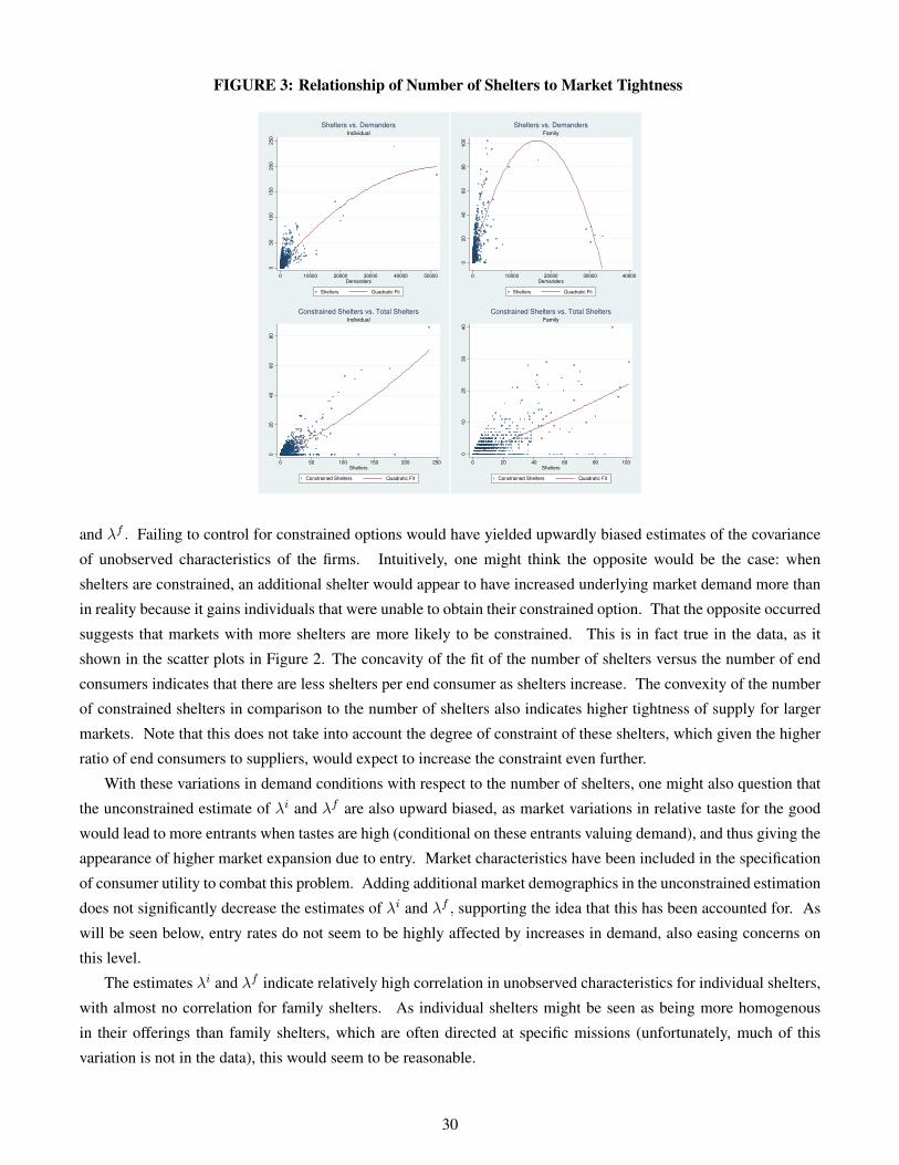
FIGURE 3: Relationship of Number of Shelters to Market Tightness

050

100

15

020

0250

0 10000 20000 30000 40000 50000

Demanders

Shelters Quadratic Fit

Individual

Shelters vs. Demanders

020

40

60

80

0 50 100 150 200 250

Shelters

Constrained Shelters Quadratic Fit

Individual

Constrained Shelters vs. Total Shelters

020

40

60

80

100

0 10000 20000 30000 40000Demanders

Shelters Quadratic Fit

Family

Shelters vs. Demanders

010

20

30

40

0 20 40 60 80 100Shelters

Constrained Shelters Quadratic Fit

Family

Constrained Shelters vs. Total Shelters

and λf . Failing to control for constrained options would have yielded upwardly biased estimates of the covariance

of unobserved characteristics of the firms. Intuitively, one might think the opposite would be the case: when

shelters are constrained, an additional shelter would appear to have increased underlying market demand more than

in reality because it gains individuals that were unable to obtain their constrained option. That the opposite occurred

suggests that markets with more shelters are more likely to be constrained. This is in fact true in the data, as it

shown in the scatter plots in Figure 2. The concavity of the fit of the number of shelters versus the number of end

consumers indicates that there are less shelters per end consumer as shelters increase. The convexity of the number

of constrained shelters in comparison to the number of shelters also indicates higher tightness of supply for larger

markets. Note that this does not take into account the degree of constraint of these shelters, which given the higher

ratio of end consumers to suppliers, would expect to increase the constraint even further.

With these variations in demand conditions with respect to the number of shelters, one might also question that

the unconstrained estimate of λi and λf are also upward biased, as market variations in relative taste for the good

would lead to more entrants when tastes are high (conditional on these entrants valuing demand), and thus giving the

appearance of higher market expansion due to entry. Market characteristics have been included in the specification

of consumer utility to combat this problem. Adding additional market demographics in the unconstrained estimation

does not significantly decrease the estimates of λi and λf , supporting the idea that this has been accounted for. As

will be seen below, entry rates do not seem to be highly affected by increases in demand, also easing concerns on

this level.

The estimates λi and λf indicate relatively high correlation in unobserved characteristics for individual shelters,

with almost no correlation for family shelters. As individual shelters might be seen as being more homogenous

in their offerings than family shelters, which are often directed at specific missions (unfortunately, much of this

variation is not in the data), this would seem to be reasonable.

30

TABLE 4: Organization Level Contribution System Estimates

(1) OLS (2) OLS (3) sysGMM (4) sysGMMlog(A1/p) log(A1/p) log(A1/p) log(A1/p)

Shelters 0.0970∗∗∗ 0.0684∗∗∗ 0.0733∗∗ 0.0653∗

(0.00739) (0.00808) (0.0370) (0.0355)

Beds 0.000967∗∗∗ 0.000801∗∗∗ 0.000238 0.00000796(0.000203) (0.000200) (0.000660) (0.00107)

Housed Individuals 0.000367 0.000297 0.000775 0.0000199(0.000264) (0.000259) (0.00101) (0.00148)

Shelter Invest/Divest 0.0935(0.0775)

Beds Invest/Divest 0.000586(0.000759)

% Emergency Shelter -1.723∗∗∗ -1.001∗∗∗ -0.944∗∗∗

(0.400) (0.341) (0.366)

% Transitional Housing -2.613∗∗∗ -1.844∗∗∗ -1.747∗∗∗

(0.396) (0.347) (0.377)

% Permanent Sup. Housing -2.029∗∗∗ -1.249∗∗∗ -1.300∗∗∗

(0.405) (0.368) (0.370)

% Fam Only -0.000279 -0.0103 0.0546(0.0624) (0.0774) (0.0848)

% Ind Only -0.177∗∗∗ -0.184∗∗ -0.0743(0.0568) (0.0740) (0.0915)

% Male Only -0.452∗∗∗ -0.393∗∗∗ -0.535∗∗∗

(0.0581) (0.0708) (0.108)

% Female Only -0.416∗∗∗ -0.369∗∗∗ -0.325∗∗∗

(0.0572) (0.0682) (0.0800)

% HIV -0.00807 -0.0163 -0.00712(0.109) (0.149) (0.173)

% Domestic Violence 0.163∗∗∗ 0.150∗∗ 0.177∗∗

(0.0602) (0.0720) (0.0859)

% Veterans -0.215∗∗ -0.237 -0.144(0.102) (0.160) (0.174)

McKinney Funding? 0.233∗∗∗ 0.198∗∗∗ 0.163∗∗∗

(0.0381) (0.0469) (0.0542)Observations 9286 9286 9286 6122R2 0.060 0.101Hansen Statistic 12.50 10.52P > chi2 (df) 0.407 (12) 0.723 (14)Arellano-Bond AR(1) Test -6.08 -4.85P > z 0.000 0.000Arellano-Bond AR(2) Test 0.73P > z 0.464Year dummies and constant also included. Standard errors in parentheses.∗ p < 0.10, ∗∗ p < 0.05, ∗∗∗ p < 0.01

Contribution System Estimates The first-stage contribution estimates (that is, for the taste parameters between

firms) are given in Table 4. One of the important questions both in terms of contributor behavior and inference on

the objective functions of firms is whether contributors have a taste for firms with more shelters, more beds, and

more individuals housed. In the OLS estimates of panels 1 and 2 of Table 4, there would seem to be a strong

taste preference among potential contributors for larger capacity firms, although not significantly for the amount of

individuals they house. This of course fails to control for the possible endogeneity of firms with higher unobserved

contribution taste effects being able to increase their capacity to higher levels, nor some relationship between the

general scope of an firm in multiple non-profit sectors and their size in the analyzed market. The system GMM

estimation in panel 3 controls for this by relying on in sample variation. The estimator of the contributor taste for

beds falls sharply in this specification and becomes insignificant (even in respect to the smaller standard errors of

the OLS estimates). The shelter taste parameter remains significant, however.

If the causality of the model is broken, and firms decide on investment decisions with knowledge of their future

contributions in hand (for example, due to a major future pledge for a donor contingent on investment), then this

taste for size might erroneously appear in these estimates. One test for this is to include the amount of realized

investment in shelters and beds in a period in the specification. This is given in panel 4, and the estimates show

no evidence for such a scenario, with the investment parameters insignificant and the capacity parameters staying

roughly the same. Therefore the data does suggest some taste for size on the shelter level among contributors.

31

TABLE 5: Market Level Contribution System Estimates

(1) OLS (2) OLS (3) sysGMM (4) sysGMMShare of GDP Share of GDP Share of GDP Share of GDP

Organizations 0.000131∗∗∗ 0.000137∗∗∗ 0.0000211 0.0000775(0.0000262) (0.0000264) (0.0000643) (0.0000857)

Organizations2 -0.00000194∗∗ -0.00000208∗∗∗ -0.000000229 -0.00000143(0.000000774) (0.000000775) (0.000000971) (0.00000206)

Organizations3 1.11e-08∗ 1.21e-08∗ 1.45e-09 9.02e-09(6.32e-09) (6.32e-09) (4.00e-09) (1.43e-08)

mean exp(XB) 0.00324∗∗ 0.00434(0.00146) (0.00272)

(mean exp(XB))2 -0.00270∗∗ -0.00336∗∗

(0.00137) (0.00166)

(mean exp(XB))3 0.000541∗∗ 0.000623∗∗

(0.000264) (0.000252)

COC GDP -4.31e-14∗ -5.17e-14∗∗ -5.66e-14∗∗ -6.22e-14∗∗

(2.48e-14) (2.50e-14) (2.47e-14) (2.61e-14)

COC GDP2 3.27e-25∗ 3.70e-25∗ 4.60e-25∗∗∗ 4.35e-25∗∗

(1.95e-25) (1.96e-25) (1.47e-25) (1.95e-25)

COC GDP3 -5.17e-37 -5.36e-37 -6.35e-37∗∗∗ -5.10e-37(4.36e-37) (4.35e-37) (2.11e-37) (4.75e-37)

Observations 1892 1892 1390 1390R2 0.1205 0.1205Hansen Statistic 17.88 33.87P > χ2 (df) 0.809 (24) 0.939 (48)Arellano-Bond AR(1) Test -1.90 -1.82P > z 0.058 0.068Arellano-Bond AR(2) Test -0.71 -0.65P > z 0.481 0.513Constant, year dummies, and cubic terms for COC PPRN, area, and size included. Standard errors in parentheses∗ p < 0.10, ∗∗ p < 0.05, ∗∗∗ p < 0.01

The second-stage contribution estimation, given in Table 5, attempts to semi-parametrically estimate the un-

known share of GDP donated to the market. Of prime importance here is the relationship between the number of

firms in the market and the overall amount of money entering the market. The OLS estimates in panel 1 and 2 imply

a concave increase in the share of GDP donated due to the number of firms. It is of interest that this function is

indeed concave: It implies that firms are indeed competing over a limited sum of donations, and thus entry does

not merely expand the amount of resources entering, but rather also steals some from other firms. Given the almost

complete lack of knowledge of substitution of contributions between firms in a market, this is an important result.

This relationship in the OLS specification between firms and resources is also suspected to be upward biased due to

the fact that firms may enter in search of contributions when the relative market taste is high. This is controlled in the

system GMM estimates of panel 3 and 4. The estimates on the effect of an additional firm on total donations fall by

an order of magnitude, and do not even approach significance. The data thus gives no evidence of market donation

expansion due to entry, and it appears that the firms are competing over an almost fixed pie in the contribution side

of the market. The inclusion of the mean of the taste parameters of firms in panel 4 also have an insignificant effect

on the share of GDP donated.

Although at first glance it may appear that the result of increased contributions attracting more firms would lend

support to the Net Revenue specification of the objective function, this is not clearly inferred. As above, firms may

be constrained from entry by a lack of funding, even if they are actually motivated by maximizing their own demand

or surplus.

Costs and Unobserved Asset Function Estimates Baseline cost estimates are given in Table 6. The linear

marginal cost specification in panel 1 shows a large fixed cost of operation, and a reasonable marginal cost of each

shelter bed. I test for quadratic terms in the cost function in panel 2. This leads to a decrease in the linear term for

both individual and family beds, and the individual bed cost actually shows the strange result of convexity in costs.

Given the noise induced by the presence of supportive service costs, and the skewness of the data in terms of costs,

there is some question of whether this is being induced by extreme outliers. In panel 3, I check this by removing

32

TABLE 6: Cost and Unobserved Asset Function Estimates

a) Baseline Costs

(1) (2) (3)Base Costs Base Costs Base Costs

Individual Beds 10760.3∗∗∗ 4055.2∗∗∗ 9925.1∗∗∗

(152.7) (330.4) (203.8)

Family Beds 8873.8∗∗∗ 7614.8∗∗∗ 11484.7∗∗∗

(332.8) (773.1) (448.1)

(Individual Beds)2 60.62∗∗∗ -46.08∗∗∗

(2.586) (1.766)

(Family Beds)2 -2.288 -79.92∗∗∗

(17.65) (10.27)

Constant 134302.1∗∗∗ 180308.1∗∗∗ 130094.9∗∗∗

(4337.0) (5552.7) (3228.7)Observations 17007 17007 16820R2 0.239 0.263 0.222Outliers (over 3 s.d. from mean) removed in spec. 3. Standard errors in parentheses∗ p < 0.10, ∗∗ p < 0.05, ∗∗∗ p < 0.01

b) Investment Costs

(1) (2)Investment Costs Investment Costs

Shelter Investment 344180.7∗∗∗ 288054.2∗∗

(80850.7) (127815.3)

Bed Investment 15738.4∗∗∗ 21041.5∗∗

(2821.1) (9760.7)

(Bed Investment)2 -76.27(134.4)

Observations 199 199R2 0.136 0.138Standard errors in parentheses∗ p < 0.10, ∗∗ p < 0.05, ∗∗∗ p < 0.01

c) Unobserved Assets

(1) (2)Unobs Asset Change t Unobs Asset Change t

Unobserved Asset Change t-1 0.951∗∗∗ 0.963∗∗∗

(0.00676) (0.00682)

Assets t-1 -0.0794∗∗∗ -0.0290∗∗∗

(0.00155) (0.00563)

(Assets t-1)2 -2.87e-11∗∗∗

(3.08e-12)

Shelter Investment/Disinvestment 201009.2∗ 236139.5∗∗

(104083.5) (114563.9)

(Shelter Inv/Div)2 15006.7(16349.5)

Bed Investment/Disinvestment 5723.0∗∗ 6522.5∗∗

(2702.4) (2785.6)

(Bed Inv/Div)2 14.91(9.585)

Constant -144383.5∗∗ -307386.8∗∗∗

(71528.0) (73222.8)Observations 6676 6676R2 0.805 0.808Standard errors in parentheses∗ p < 0.10, ∗∗ p < 0.05, ∗∗∗ p < 0.01

the outliers in terms of the dependant variable (defined as being over three standard deviations from the sample

mean) and the result is linear terms similar to the model in panel 1, and significant but economically small (under

100 dollars per bed) economies of scale in individual and family beds. Given the questionable nature of removing

outliers, the uncertainty in the effect of scale on marginal costs, and the original postulation of linear marginal costs

in the model, I choose to retain the linear marginal costs in panel 1. I explain the noise in the estimates indicated

by a low R2 value to be a result of the presence of variable supportive service costs, which as discussed above are

observed in the unobserved asset function.

Investment cost estimates are given in the second subtable. As stated above, all data on investments are from

firms that are building new shelters. Thus, I treat the fixed cost in this estimate as the cost of building a shelter, and

in panel 1, specify a linear cost of each bed. I test in panel 2 for an effect of economy of scale, but find no significant

effect. Again, the R2 value is low, which I justify by treating investment costs as random shocks. Although it

may be superior to control for some differences in input costs between markets, the small size of the investment

data relative to the firm data set, and the non-uniform jurisdictional areas of the markets unfortunately makes this

infeasible.

The unobserved asset function estimates are given in the third subtable. Note that unobserved assets are al-

most always negative, with as expected unobserved costs exceeding unobserved revenues (contributions are always

observed). Unobserved assets show strong serial correlation from one period to the next, and their relationship to

current asset levels and investment patterns are similar to what might be expected. Unobserved assets decrease

(that is, become more negative) when the asset levels are higher, thus implying higher net outlays when firms have

more funds. When shelters increase (decrease) their capacity in shelters and beds, this increases (decreases) their

unobserved asset levels. This implies that firms are actively shifting their spending between different sectors and/or

between capacity and supportive services, as might be expected. Although investigating the possible substitution

between different variables of service provision (in this case, capacity and supportive services) is an interesting

question, data limitations lead it to be outside the scope of this paper.

Policy Functions

33

TABLE 7: Reduced Form Organizational Investment Policy Functions

Individual Family(1) (2) (3) (4) (5) (6)

Invest Beds Invest Beds Invest Beds Invest Beds Invest Beds Invest Beds(Homeless by Type)/Shelters (COC) 0.0230∗ 0.0307∗ 0.0310∗ 0.000281∗ -0.0000311 -0.000127

(0.0126) (0.0169) (0.0169) (0.000160) (0.000194) (0.000191)

Unsheltered Homeless by Type -0.0334∗ 0.00299 0.00230 -0.0175 -0.00175 0.00198(0.0181) (0.0233) (0.0233) (0.0191) (0.0238) (0.0238)

Occupancy % (Org) 0.0247∗∗ 0.0191 0.0190 0.0291∗∗ 0.0204 0.0196(0.0103) (0.0132) (0.0132) (0.0119) (0.0151) (0.0151)

Beds by Type (Org) -0.191∗∗∗ -0.291∗∗∗ -0.292∗∗∗ -0.00435 -0.242∗∗∗ -0.249∗∗∗

(0.0164) (0.0205) (0.0205) (0.0190) (0.0277) (0.0276)

Shelters by Type (Org) -0.00464 0.0387 0.0387 -0.00737 0.0643∗∗∗ 0.0683∗∗∗

(0.0202) (0.0237) (0.0237) (0.0193) (0.0235) (0.0235)

All Beds (Org) -0.0221 0.0293 0.0289 -0.348∗∗∗ -0.0153 -0.00742(0.0159) (0.0192) (0.0192) (0.0164) (0.0327) (0.0326)

All TH Shelters (Org) 0.00340 -0.0176 -0.0180 0.106∗∗∗ 0.00843 0.00567(0.0221) (0.0257) (0.0257) (0.0231) (0.0296) (0.0296)

McKinney Funding? (Org) 0.00569 0.00684 0.00687 0.00685 0.0267∗ 0.0270∗

(0.0103) (0.0128) (0.0128) (0.0121) (0.0151) (0.0152)

Total Shelters (Org) -0.00396 -0.00236 -0.00258 0.00791 -0.0164 -0.0196(0.0144) (0.0166) (0.0166) (0.0185) (0.0220) (0.0221)

Contributions t -0.0560 -0.0581 -0.0227 -0.0213(0.0430) (0.0430) (0.0454) (0.0454)

Contributions t-1 0.0585 0.0575 0.0316 0.0267(0.0431) (0.0430) (0.0450) (0.0450)

Assets 0.00189 0.143∗∗∗

(0.0474) (0.0393)

Liabilities 0.00434 -0.143∗∗∗

(0.0493) (0.0384)

log(Net Assets+3e08) 0.0154 0.0439∗∗

(0.0134) (0.0175)

COC Total Income 0.189∗∗ 0.120 0.118 0.0776 0.269∗∗∗ 0.260∗∗∗

(0.0789) (0.0952) (0.0951) (0.0827) (0.0998) (0.0999)Observations 6453 3935 3935 5236 3402 3402R2 0.059 0.087 0.087 0.162 0.082 0.080Constant, CoC population, area, and PPRN also included.

Coefficients are standardized to reflect changes in standard deviations. Standard errors in parentheses

Type is either Family or Individual based on market type. Constant added to Net Assets to ensure real logarithm.∗ p < 0.10, ∗∗ p < 0.05, ∗∗∗ p < 0.01

Reduced Form I begin my analysis of firm behavior by looking at what can be inferred from reduced form

specifications of the policy function. The advantage of these specifications is that they are freed from any of

the assumptions of the structural model. The disadvantage is that as discussed above, they often fail to lead to

clean inference between different specifications of the objective function. Their static nature also fails to control

for expectations of future structure that should affect firm decision making, nor allows for analysis of long-term

responses to market shocks.

In Table 7, I present several specifications of the function of a firms investment decision conditional on it staying

in the market, be it positive, negative, or zero. In Table 8, I present specifications for exit probabilities, and in Table

9, specifications for the number of entrants. The value EXIT = 1 corresponds to the firm leaving the specific

market, be it individual or family, and not that it necessarily folded as a entity altogether. I include several important

variables that would support different objective functions for firms. The ratio of homeless persons of the firms type

(be it family or individual) to the number of shelters by type would indicate the presence of additional demand that

could be captured by a firm by investment, entry, or not exiting. A correlation of this variable with the firm’s actions

would support both Own Demand and Market Surplus specifications of firm utility. Correlation with the number of

unsheltered individuals in the market would also support both these specifications, although controlling for the other

variables it should skew towards the Market Surplus specification, as this would indicate a higher marginal utility

due to taking people from the streets as opposed to other shelters.

Two caveats of this interpretation are in order. Firstly, if a firm already has spare capacity, that is, more beds

than are being demanded, they may not increase their capacity in response to the presence of more individuals in the

34

TABLE 8: Reduced Form Organizational Exit Policy Functions

Individual Family(1) (2) (3) (4) (5) (6)

%Mfx %Mfx %Mfx %Mfx %Mfx %Mfx(Homeless by Type)/Shelters (COC) -.1510155∗∗ -.078954 -.0782966 .0007581 .0006561 .000774

(.0663658) (.1099665) (.1099549) (.0007259) (.0012496) (.0012284)

Unsheltered Homeless by Type -.0541202 -.1376858 -.1353058 .3250557∗∗∗ .4233594∗∗∗ .4104445∗∗∗

(.0793894) (.163836) (.1638282) (.063446) (.1032996) (.1026421)

Occupancy % (Org) .0108798 .044533 .0471241 -.0021122 -.0986882 -.100151(.047225) (.0760833) (.0760813) (.0589304) (.0888423) (.0887352)

Beds by Type (Org) .2862418∗∗ .2282431 .2323787 .0071519 -.006273 .0178622(.1452509) (.2011192) (.2019944) (.1519301) (.2218857) (.2239047)

Shelters by Type (Org) -.2359088∗ -.2553821 -.2596215 -.1238878 .0816008 .0935237(.1214631) (.1768661) (.1771799) (.1323069) (.1969951) (.1989978)

All Beds (Org) -.4431815∗∗∗ -.1988267 -.1956298 -.1918838 -.0677982 -.0994937(.1564112) (.19463) (.1957032) (.1845419) (.2692614) (.2745309)

All TH Shelters (Org) .486238∗∗∗ .2124421 .2124748 .3386276∗∗ -.1716061 -.2905552(.1412498) (.1925702) (.1928529) (.1493309) (.2432738) (.2118623)

McKinney Funding? (Org) -.4411632∗∗∗ -.422567∗∗∗ -.4249264∗∗∗ -.2993008∗∗∗ -.3352507∗∗∗ -.3353765∗∗∗

(.0585258) (.0855138) (.0855202) (.0648713) (.100395) (.1002256)

Total Shelters (Org) -.7521458∗∗∗ -.3771415∗∗∗ -.3725827∗∗∗ -.6584362∗∗∗ -.1402226(.1230554) (.1416563) (.1424597) (.1345587) (.1515275)

Contributions t .155125 .1657519 -.0668709 -.084903(.2674156) (.270814) (.353034) (.3522475)

Contributions t-1 -.119681 -.1014186 .1018822 .1149244(.2730338) (.2767734) (.344726) (.343486)

Assets -.6799932 -.1339174(.4477633) (.3021575)

Liabilities .4601587∗∗ .1828785(.1963969) (.2787057)

log(Net Assets+3e08) -.2247973∗∗ .0041043(.1022606) (.124645)

COC Total Income -1.368975∗∗∗ -1.539104∗∗ -1.522838∗∗ .4231241 .496539 .4907157(.4032475) (.6185543) (.6182097) (.4086952) (.6322736) (.6297348)

Observations 6453 3935 3935 5236 3402 3402Baseline Probability .0442173 .0429241 .0429304 .0350994 .0338946 .0339015Psuedo-R2 .0594 .0484 .0480 .0456 .0452 .0438Constant, CoC population, area, and PPRN also included.

Reported parameters are percentage effect of one standard deviation change in independent variable. Standard errors of Mfx in parentheses

Note: Type is either Family or Individual based on market type. Constant added to Net Assets to ensure real logarithm.∗ p < 0.10, ∗∗ p < 0.05, ∗∗∗ p < 0.01

market, as long as their capacity still exceeds this increased demand. Thus, only firms with constrained or nearly

constrained capacities should increase their number of beds or shelters in response to demand shocks. For this

reason, I also include in the specifications the number of beds and shelters of a firm, and the percentage occupancy

at the current date.

Secondly, if firms are constrained financially, they will not be able to increase their capacities, even if they would

like to increase their own demand or marginal market surplus. In fact, the effect of contributions and asset levels on

behavior can be supportive of different specifications depending on the action type and the constraints faced by the

firms. For the Own Demand and Market Surplus specifications, contributions and assets will have a high effect on

investment if firms are constrained in terms of output by the amount of money they have on hand or plan to receive.

If they are constrained in terms of output by the demand for their services, however, increasing contributions and

assets will not affect their investment levels. The same holds true for exit and entry: the affect of money can be

very important if is indeed constraining output, but an infinite amount of money is not useful to a firm seeking to

maximize output or affect surplus if their are no end consumers to serve with this money.

In terms of investment, if firms’ utility corresponds with the Net Revenue interpretation, there should be little

effect of asset or contribution levels on investment. Entry and exit, on the other hand, should be heavily influenced

by contribution streams, as firms would only forgo their outside option if there was a sufficient amount of net revenue

to acquire.

In what will become a running theme throughout the analysis, the overall implication of the data is not so much

strong evidence parsing between the alternative specifications of the objective functions, but rather that none of the

35

TABLE 9: Reduced Form Organizational Entry Policy Functions

Individual Family(1) (2) (3) (4)

Entrants Entrants Entrants Entrants(Homeless by Type)/Beds COC 0.101∗∗ 0.0616

(0.0401) (0.0428)

I(Homeless by Type)/Shelters COC 0.0771∗ 0.0508(0.0406) (0.0435)

Unsheltered Homeless by Type -0.0569 -0.0370 -0.00806 -0.00556(0.0499) (0.0450) (0.0439) (0.0416)

COC Total Orgs 0.632∗∗∗ 0.647∗∗∗ 0.571∗∗∗ 0.572∗∗∗

(0.0557) (0.0555) (0.0599) (0.0590)

Average Incumbent Contributions -0.0315 -0.0552 -0.0379 -0.0404(0.0421) (0.0471) (0.0404) (0.0407)

COC Total Income -1.188∗∗∗ -1.241∗∗∗ -0.553∗∗ -0.552∗∗

(0.230) (0.231) (0.252) (0.248)

Area Total -0.0680∗∗ -0.0734∗∗ -0.0549 -0.0555(0.0333) (0.0333) (0.0356) (0.0357)

Population Total 1.212∗∗∗ 1.263∗∗∗ 0.656∗∗∗ 0.661∗∗∗

(0.228) (0.229) (0.249) (0.247)

PPRN amount -0.107∗ -0.106∗ -0.160∗∗ -0.143∗∗

(0.0610) (0.0610) (0.0674) (0.0653)

Constant 0.0403 0.0508 0.0686 0.0651(0.0745) (0.0702) (0.0753) (0.0723)

Observations 547 539 546 539R2 0.312 0.323 0.255 0.260Coefficients are standardized to reflect changes in standard deviations. Standard errors in parentheses

Note: Type is either Family or Individual based on market type.∗ p < 0.10, ∗∗ p < 0.05, ∗∗∗ p < 0.01

proposed specifications are clearly supported by the data to be the driving force of decision making. In the num-

ber of investment beds determinants in Table 7, firms in individual markets show significantly higher investment

when the ratio of homeless individuals to shelters is higher. Of note is the fact that these values, though signifi-

cant, are economicaly small. Standardized coefficients are reported, indicating a standard deviation change in the

Homeless/Shelter ratio increases predicted investment by under .031 standard deviations for each specification. The

confidence intervals on these values are fairly tight, supportive of only a small effect of differences in demand. The

values are similarly small for investment of firms in family markets, and only significant when financial variables are

not included. The amount of unsheltered homeless are not significant either statistically or economically for either

group of firms. In either case, the included variables are not highly predictive of behavior.

In Table 8 I present a marginal percentage change on the likelihood of exit due to a standard deviation change

in the independant variable (a semi-elasticity), and in Table 9 again report standardized coefficients. The effect of

these two variables on exit and entry rates is not always directionally supportive of maximization of own demand

or surplus maximization, and again not supportive of being an important driver of behavior. Increases in the home-

less/beds ratio and the amount of unsheltered homeless for individual markets generally decrease exit probabilities

and increase entry rates, but are only sporadically significant and are again economically small. In family markets,

the effects are of similar magnitude but for exit are in the opposite direction, in several cases significantly. This may

suggest some unobserved differences in markets not accounted for by the reduced firm model, which I will attempt

to rectify in the more complete structural specification. The occupancy percentage of a organization, which would

imply more utility if firms were own provision pr ,market surplus maximizing, does not significantly explain exit

rates.

Again, I have pointed out two explanations why these market demand variables may not affect behavior: firms

may already have enough capacity to satisfy increased demand, or may be financially constrained and thus not

be able to respond to demand shifts. There does not appear to be strong evidence for either of these scenarios.

Controlling for a number of capacity variables for the firm, the percentage occupancy of the firm (which would

indicate capacity tightness) has a insignificant and tighly small effect on capacity investment for all specifications.

36

The effect of occupancy on exit would be unaffected from these constraints, and again is insignificant.

The effect of assets and liabilities on investment are directionality supportive of financially constrained firms,

but are mainly insignificant and again relatively small. Given the wide range of assets between firms, the standard

deviation change is very large numerically. As ane example, It would take somewhere on the order of a billion dollars

to increase the amount of expected investment by one bed. Since investment cost of a bed is estimated to be roughly

$16000, it is not highly supportive of tight financial constraints on growth. I also include a specification with logged

net assets, shifted by a constant such that the log is always a real number. Again, this finds very small effect on

investment, with the average net asset level of $3.6 million having to be increased to $53 million (individual) and

$22 million (family) to expect one more invested bed.

If there is not strong evidence that firms make decision to increase demand or surplus, than this is supportive

of firms being solely concerned with net revenues, or “for-profits in disguise”. If this were the case, however, we

would expect exit and entry to be affected by prospective inflows of revenue. The affect of revenue inflows, that is

contributions, on exit is insignificant. The level of assets and liabilities is significant for individual firms, but not

for family firms, and is again relatively small. Even this significance does not imply entry and exit in the search for

revenue flows: lower levels of net assets could just as easily imply a lack of money available to fulfill demand, or to

remain solvent as an entity altogether.

Entry rates are also not significantly affected by demand variables, or variables such as CoC income or the

average contribution level of incumbent firms which may indicate the presence of additional funds for entrants.

Higher average contribution levels of course could also indicate incumbents with high contribution taste levels, thus

making revenues harder to come by for entrants. I again will attempt to control for this in the structural model.

Structural Attempting to gain inference on utility specifications from the structural policy functions without

the context of the transition of the state space suffers from many of the same pitfalls as the reduced form policy

functions. In particular, their static nature fails to control for expectations of future market states. The presence of

first stage structural parameters, however, allows for greater controls on the actual market structure in the estimation

period.

The estimates of the structural policy functions echo many of the insights of the reduced form policy functions:

firms have small and usually insignificant responses to market parameters affecting demand, surplus, and contribu-

tions. The larger confidence intervals induced by controlling for errors in first stager parameter estimation lead to

even less significant relationships between market and firm parameters and firm behavior.

The structural policy functions do, however, offer more but still not convincing support for financially con-

strained firms who which to maximize some measure of demand. The investment decision functions in Table 15

(given in the additional table section) are ordered logit models with three choices: to disinvest in capacity, stay at

the current level of capacity, or invest in capacity. The level of net-assets significantly increases the probability

of investing, both for individual and family firms. It does not, however, significantly affect exit probabilities or

investment or divestment quantities. For individual firms, the higher the level of the market sum of firm contribution

taste parameters log(∑n∈mt

A1/pnmt) , the significantly lower the probability of investment, which would be indicative

of investment in the presence of less competition for funds in the market. In another somewhat strange result, the

higher the number of market shelters, the higher the propensity to invest. Since the model controls for the market

sum of end consumer taste parameters log(∑s∈mt

exp( Vsmt1−λk )), this may indicate less competition for demand, but if

37

this was the case, we would expect at least a negative coefficient on log(∑s∈mt

exp( Vsmt1−λk )), which we do not. In any

case, even if firms are attempting to maximize their output or market surplus but are financially constrained from

doing so, the market shock response simulations below will show that this response is very small in comparison to

the size of the shocks.

State Space Transitions The state space transitions offer yet another look at firm responses to changes in market

structure, this time at the market level. An immediate insight is that higher levels of supply, be it in terms of beds,

shelters, or firms, do not have a significant effect on the number of end consumers in the following period. Again,

as in the policy functions, the more shelters in the market, the higher expected number of beds in the next period.

None of the capacity measures are significantly affected by the current level of demand, nor the estimate of market

tightness Ω, echoing the lack of market response to demand shocks implied above.

The state space variables∑n∈mt

Anmt1/(1−ρ),

∑s∈mt

exp( Vsmt1−λk ),Ωmt, and CSmt, which are modeled as functions

of the other transitioning state space variables, show the relationships that would be expected from the structural

model. This is important as in the simulation they are estimated as a projection of the transitioning variables by

these functions. The market sum of contribution taste parameters log(∑n∈mt

Anmt1/(1−ρ)) increases significantly with

the logged number of market firms. The market sum of demand taste parameters log(∑s∈mt

exp( Vsmt1−λk )) increases

significantly with higher numbers of market shelters and also with the market demand error. It also is positively

correlated with the number of market beds and negatively correlated with the number of end consumers. This results

from correlation with these values with the market demographic taste parameters estimated in the demand system.

The estimate of market tightness Ωmt is positively correlated with the number of demanders and negatively correlated

with the number of beds, as would be expected. Finally, the estimate of consumer surplus per end consumer CSmtis also positively correlated with the number of demanders and negatively correlated with the number of beds.

Each of these variables also show relatively high levels of serial correlation in terms of their deviations with their

expected values based on the transitioning state space variables, as related by the serial correlation terms ρ. This

indicates the expected serial correlation of market structure not explained by the transitioning state space variables

Imt,Jmt,∑n∈mt

Qnmt,∑n∈mt

Shnm and Nmt.

7.2 Dynamic Estimates

As stated above, I estimate 30 different specifications of the objective function being maximized by firms. First,

assuming normal shocks to the utility of each action, I estimate a model of utility only including a constant to reflect

the value of being entered, with the outside option normalized to Y=0. I then estimate linear specifications for

all possible omission and inclusion combinations of these three terms, for 7 models in total. Finally, I estimate

specifications under the same combinations with a cubic term for each omitted variable, and a interaction term for

all linear included terms, for 7 further specifications. This is repeated under the assumption of Type-1 Extreme

Value errors, for 30 specifications in total.

The estimates of the objective function parameters are reported for the assumption of normal shocks to utility

in Table 12. I do not report the values for T1EV errors, as they turned out to be quite similar. As one can see

in the table, none of the parameters estimated is significant with respect to the bootstrapped confidence intervals.

Additionally, nothing can be inferred from the size of these parameters, as the utility function has been scaled and

normalized by the restriction of the outside option to Y=0 and the standard deviation of 1 for the normal errors to

38

TABLE 10: Individual State Space Transition

log(COC Income t+1) log(Market Demanders t+1) log(Market Beds t+1) log(Market Shelters t+1) log(MarketOrgs t+1)β 95% CI β 95% CI β 95% CI β 95% CI β 95% CI

Constant .92037 -.084852 2.9778 1.9143 -4.22016 2.21382 5.0721 -1.25012 7.22278 -.17131 -3.61774 2.04998 -.73677 -3.08076 .751054log(COC Income) .96006 .871034 1.00364 -.057056 -.0771558 .239008 -.20611 -.316526 .073358 .0069617 -.108204 .162152 .038754 -.0246888 .150998log(Market Demanders) .54852 .374064 .742232 .17897 -.043995 .352174 .0037746 -.103216 .190132 .041302 -.0377996 .127092log(Market Beds) -.027705 -.0922054 .0513678 .38427 .22707 .642552 .0045792 -.0973196 .0824862 -.029119 -.104256 .0433994log(Market Shelters) .089157 -.0864236 .255154 .64472 .233856 .726604 .77728 .571636 .917638 .091787 -.0295888 .219514log(Market Orgs) .15783 -.177514 .332836 .12049 -.12204 .503716 .16914 -.0613792 .394744 .8356 .610096 .990224log(sum A1/p) -.10626 -.150762 .019365 -.025196 -.179426 .106852 .031694 -.0900158 .13724 .046816 -.0158186 .0961348log(sum V) -.01948 -.0831616 .0370012 .019545 -.0480766 .0905204 .038139 -.0211268 .080122 .0031325 -.0182982 .03593881/omega .066429 -.146444 .192354 .027478 -.147816 .292286 .16629 -.146838 .213772 .051501 -.0788856 .123498log(Market Surplus) -3.1581 -15.4316 4.3999 .66279 -9.54896 9.75892 2.7404 -8.440559 11.5122 2.8735 -1.57746 6.88196Market Demand Effect -.04472 -.18548 .046679 .24829 .0276126 .373206 -.039891 -.148592 .0836058 .0064499 -.0804822 .0520884Market Contributions Effect -3.4574 -8.458159 5.17978 .20035 -9.169519 18.3964 -2.37 -7.49936 8.42886 3.5727 -3.2642 8.7543log(Lag Market Demanders) .28521 .138588 .388476 -.047692 -.178566 .131842 .01687 -.106202 .129812 -.022097 -.0662138 .069181

log(sum A1/p) log(sum V) (1/omega) log(Market Surplus/Demanders)β 95% CI β 95% CI β 95% CI β 95% CI

Constant -1.4116 -3.6512 -.2419482 7.6462 1.92612 43.3992 -1.123 -2.49736 .935928 3.4573 3.41764 3.48414log(COC Income) .035698 -.0290496 .11954 -.39186 -2.29816 -.1153156 .11666 .0166708 .179588 -.0017816 -.0033498 .0004963log(Market Demanders) -.047627 -.110078 .0390362 -.90047 -1.68446 -.714398 -.37243 -.40145 -.25312 -.0069702 -.0086467 -.005398log(Market Beds) -.014341 -.0634112 .0603294 .88061 .652656 1.81078 .32902 .238588 .362546 .0063517 .0052788 .0075976log(Market Shelters) .074448 -.139054 .215902 .59399 .38395 1.42664 -.11279 -.192112 -.0063278 .0016453 -.0005228 .0037398log(Market Orgs) 1.0772 .895414 1.26218 -.063767 -.58898 .419552 -.040276 -.107892 .09099 .000518 -.0026557 .0023559log(sum A1/p) -.031756 -.0840806 .017317 .0000506 -.0008849 .0008048log(sum V) -.034399 -.096206 .0296346 .0028714 .0003869 .00439161/omega .0010074 -.003019 .0046307log(Mean Market Surplus)Market Demand Effect 1.2378 .466404 12.401 .032466 -.0526964 .208676 .0099167 .0050355 .0140844Market Contributions Effect -3.4846 -10.5566 7.0439 -.023974 -.176606 .0882896log(Lag Market Demanders)Rho .516 .363975 .657725 .243 .10545 .41705 .418 .2799 .503 .638 .2836 .7351

TABLE 11: Family State Space Transition

log(COC Income t+1) log(Market Demanders t+1) log(Market Beds t+1) log(Market Shelters t+1) log(MarketOrgs t+1)β 95% CI β 95% CI β 95% CI β 95% CI β 95% CI

Constant .92037 -.084852 2.9778 -1.7815 -6.0438 .756356 .29591 -3.51668 2.94666 -.86196 -2.79346 1.41104 -.85538 -2.86716 .199052log(COC Income) .96006 .871034 1.00364 .12156 .0190025 .343324 .024029 -.103052 .200034 .022668 -.0817752 .112792 .03762 -.0094058 .13647log(Market Demanders) .71911 .476224 .854722 .018858 -.0888992 .138742 .015037 -.0446542 .144238 .026684 -.042842 .0799438log(Market Beds) .019032 -.130568 .162254 .59693 .519602 .750878 .071839 -.0318766 .136344 -.013673 -.0676946 .048179log(Market Shelters) -.014621 -.0912868 .224026 .20183 .0983738 .37093 .78937 .63035 .907352 .037013 -.0325776 .115166log(Market Orgs) .15637 -.16349 .237788 .22408 -.0512926 .307518 .044887 -.0335602 .223088 .84846 .7372 .952844log(sum A1/p) -.074614 -.160406 .086201 -.050595 -.132876 .030563 -.021083 -.0923536 .0930602 .037214 -.0385846 .070361log(sum V) -.04217 -.072517 -.01044 .000485 -.0107368 .0198848 -.0009236 -.0173438 .0141112 -.0004775 -.0103073 .00936271/omega -.13448 -.348146 .145804 -.0025362 -.131496 .28219 .026784 -.163114 .157732 .080047 -.0379956 .172412log(Mean Market Surplus) 2.2883 -1.72458 6.89162 .90073 -1.567 3.25838 .36458 -.984074 4.1752 -.40333 -1.79484 1.4511Market Demand Effect -.01784 -.13749 .0533608 .075355 .0156866 .181418 .013102 -.0470354 .0547288 -.0003184 -.051081 .0330262Market Contributions Effect 5.2041 1.298204 18.0902 2.0691 -2.94246 12.0224 1.7377 -3.99892 7.90104 3.7691 -3.89492 6.85174log(Lag Market Demanders) .021638 -.0651688 .140782 .02002 -.0581274 .120206 .037001 -.0418166 .0915974 .027543 -.0226856 .0775304

log(sum A1/p) log(sum V) (1/omega) log(Market Surplus/Demanders)β 95% CI β 95% CI β 95% CI β 95% CI

Constant -.69478 -2.56506 .503374 4.3134 -1.36614 15.6976 -1.3446 -2.55098 .58686 3.5045 3.44346 3.54462log(COC Income) -.013618 -.0644694 .0433484 -.20735 -.776072 .0983048 .10857 .0204104 .164352 -.0037648 -.0058526 -.0009505log(Market Demanders) .038335 -.0132444 .109792 -1.5962 -2.4747 -1.19446 -.30393 -.420332 -.260174 -.013069 -.0152458 -.0094701log(Market Beds) -.0080272 -.0591494 .10668 1.4721 1.0867 2.4207 .26067 .218814 .352358 .015568 .0108556 .0169696log(Market Shelters) .11899 -.0872838 .238098 .7361 .294414 1.28482 -.072392 -.136734 -.000413 .0036461 -.0002589 .0078351log(Market Orgs) 1.0029 .885622 1.1721 .3614 -.288436 1.20192 .0070794 -.065614 .0694278 -.0012964 -.00335 .0023888log(sum A1/p) -.022993 -.0385496 .0157896 .0008183 -.000988 .0029391log(sum V) .048186 .0262778 .0599992 .0030701 .0019725 .00397131/omega .002193 -.0112052 .0089551log(Mean Market Surplus)Market Demand Effect .9471 .603988 3.65268 .12502 .0059762 .156364 .012389 .0096241 .0178316Market Contributions Effect -3.4229 -6.9524 2.76836 -.23523 -.568068 .0045564log(Lag Market Demanders)Rho .523 .3919 .612025 .25 .09595 .375325 .484 .266375 .537925 .408 .213375 .45785

39

the utility of each action.

Despite the fact that each parameter is individually not significantly different from zero, it could be the case that

some of the parameters are jointly distinct from zero, thus indicating that the parameters included explained firm

behavior better than the model with only a constant value of being entered. Usual tests of joint significance such

as the likelihood ratio test are not applicable in this case as a result of the first stage errors, clustering of errors on

markets, and clustering of the utility shocks within firms (these are all accounted for by the bootstrap) leading to

a potentially different distribution of the estimator under the null hypothesis than what is required by these tests.

As such, I estimate rectangular joint confidence regions for the parameters via the bootstrapped distributions of the

estimator. For a confidence level α, this forms the joint confidence region for parameters x1, x2, ..., xI:

JCR(x1, x2, ..., xI) = x1, x2, ..., xI s.t. maxi

|xi − xi|σBOOTxi

< CBOOT1−α

where xi is the estimated parameter, σBOOTxi is the standard deviation of each estimator in the bootstrap distri-

bution, and CBOOT1−α is the 1-α percentile of the distribution of CBOOT1−α = maxi|xBOOTi − xi|, with xBOOT =

xBOOT1 , xBOOT2 , ..., xBOOTI being the set of estimators for each bootstrap run. From this distribution I deduct

the confidence percentage that each of the sets of unrestricted parameters compared between each unrestricted and

restricted specification is not jointly zero. These estimates are given in Table 13 and Table 14. As one can see,

none of the single or joint parameter regions even approach significance. Thus, I find no evidence from the dynamic

estimation supporting Net Revenues, Own Demand, or Market Surplus entering the objective function of firms in

the market.

8 Simulations of the Effect of Shocks on Market StructureAlthough the utility specifications show no significant evidence for any of the specified values entering the firm

utility specifications, I am still able to run simulations of responses on the market and firm level to changes in market

structure. This is achieved by administering shocks to the state space variables, and forecasting the estimated market

response over time to these shocks. The estimated responses come from the estimated state space transitions and

policy functions, and are completely distinct from any estimation of the objective function of firms.

The first set of responses to shocks are estimated on the market level. These are given in Figure 4. I begin each

simulation in the steady state of the estimated state transition function. Recall that this has been restricted to the

mean values of the state variables. I report responses to shocks as the ratio of the value of each term to its value in

this steady state. Confidence intervals are formed from running the same simulation for every bootstrapped value

of the state transition parameters estimated above.

In the first row of Figure 4, I add a one period 25% positive shock to the number of end consumers in the market.

Thus, the graph of the predicted number of market beds over the next 10 years is an impulse response function to

this shock. As can be seen, the predicted response of the number of market beds to this 25% shock is quite small.

Although the shock dissipates somewhat slowly, the number of market beds is estimated to never increase more than

5% for individual markets, and even less for family markets. As can be seen by the confidence bounds, this shock

is insignificant, and even at its most optimistic level only increases by 10% in response to the shock.

Under the specified state transitions, firms know that this shock is transitory and thus may not have enough in-

centive in terms of future discounted own provision or marginal surplus to overcome the cost of capacity investment.

40

TAB

LE

12:O

bjec

tive

Func

tion

Spec

ifica

tion

Est

imat

es

12

34

56

78

β95

%C

Iβ

95%

CI

β95

%C

Iβ

95%

CI

β95

%C

Iβ

95%

CI

β95

%C

Iβ

95%

CI

Ent

ered

Val

ue.1

2684

.110

174

.207

796

.149

79.1

0865

8.2

0953

2.1

2675

.071

6402

.181

424

.116

41.1

1104

2.2

0154

.134

73.0

7171

52.1

7872

4.1

3799

.108

466

.202

626

.117

84.0

6612

82.1

7856

.127

98.0

6701

88.1

7777

Net

Rev

enue

-7.6

3e-1

1-5

.11e

-10

3.74

e-09

-1.2

3e-1

0-7

.20e

-10

2.99

e-09

-8.0

4e-1

1-5

.94e

-10

2.98

e-09

-1.1

9e-1

0-6

.67e

-10

2.69

e-09

Ow

nPr

ovis

ion

.000

0249

-.000

1821

.008

2117

.001

2142

-.000

24.0

0771

3-.0

0005

92-.0

0022

49.0

0818

17.0

0102

67-.0

0038

35.0

0709

48M

arke

tSur

plus

7.49

e-06

-1.0

2e-0

6.0

0002

358.

51e-

06-2

.09e

-06

.000

0183

7.54

e-06

-1.9

5e-0

6.0

0002

186.

88e-

06-3

.32e

-06

.000

0182

12

34

56

78

β95

%C

Iβ

95%

CI

β95

%C

Iβ

95%

CI

β95

%C

Iβ

95%

CI

β95

%C

Iβ

95%

CI

Ent

ryV

alue

.126

84.1

1016

6.2

1032

6.1

5679

.106

74.2

2001

2.1

0976

.059

3436

.190

35.1

0846

.106

792

.200

73.1

3943

.059

6924

.192

18.1

3697

.099

877

.202

384

.101

67.0

5826

36.1

8274

8.1

3355

.055

609

.186

466

Net

Rev

enue

-5.3

7e-1

0-3

.71e

-09

5.01

e-09

-3.7

9e-1

0-3

.73e

-09

6.18

e-09

-4.6

5e-1

0-4

.05e

-09

6.12

e-09

-5.0

1e-1

0-3

.24e

-09

6.15

e-09

Net

Rev

enue∧2

-8.3

0e-2

0-1

.48e

-17

3.97

e-17

4.54

e-20

-1.8

9e-1

72.

60e-

17-1

.70e

-19

-1.7

9e-1

74.

93e-

171.

00e-

19-1

.40e

-17

3.04

e-17

Net

Rev

enue∧3

5.48

e-28

-4.5

7e-2

62.

20e-

261.

90e-

28-2

.02e

-26

1.43

e-26

5.60

e-28

-4.6

8e-2

62.

26e-

262.

66e-

28-2

.31e

-26

2.19

e-26

Ow

nPr

ovis

ion

.003

3465

-.004

357

.011

3204

.002

3652

-.004

0931

.012

4952

.002

0373

-.004

183

.009

2966

.000

4273

-.004

2898

.011

7538

Ow

nPr

ovis

ion∧

2-.0

0005

8-.0

0015

44.0

0013

78-.0

0004

01-.0

0015

27.0

0013

76-.0

0004

-.000

1496

.000

153

4.20

e-06

-.000

1482

.000

1358

Ow

nPr

ovis

ion∧

32.

09e-

07-1

.90e

-07

8.26

e-07

1.45

e-07

-1.9

0e-0

76.

32e-

071.

45e-

07-1

.97e

-07

7.94

e-07

-5.3

4e-0

9-1

.73e

-07

6.31

e-07

Mar

ketS

urpl

us.0

0001

56-.0

0001

25.0

0004

1.0

0001

68-.0

0001

13.0

0003

76.0

0001

56-9

.82e

-06

.000

033

.000

0144

-.000

0114

.000

0334

Mar

ketS

urpl

us∧2

-1.3

2e-1

1-1

.57e

-10

1.20

e-10

-1.6

5e-1

1-2

.26e

-10

1.43

e-10

-1.4

7e-1

1-1

.77e

-10

8.32

e-11

-1.2

5e-1

1-2

.38e

-10

5.12

e-11

Mar

ketS

urpl

us∧3

3.65

e-18

-3.7

6e-1

63.

29e-

166.

48e-

18-3

.80e

-16

4.07

e-16

5.35

e-18

-3.7

2e-1

64.

11e-

164.

45e-

18-2

.54e

-16

4.82

e-16

Net

Rev

enue

*O

wn

Prov

isio

n1.

65e-

12-4

.56e

-11

4.25

e-11

6.84

e-13

-1.8

2e-1

14.

23e-

11N

etR

even

ue*

Mar

ketS

urpl

us-2

.33e

-17

-1.2

9e-1

42.

53e-

14-3

.95e

-17

-1.2

4e-1

42.

20e-

14O

wn

Prov

isio

n*

Mar

ketS

urpl

us2.

09e-

10-1

.07e

-08

2.50

e-08

-1.1

3e-0

9-9

.65e

-09

2.63

e-08

TAB

LE

13:C

onfid

ence

Perc

enta

gest

hatR

estr

icte

dVa

riab

lesa

reno

tJoi

ntly

Zer

o(L

inea

rSp

ecifi

catio

ns)

Unr

estr

icte

dM

odel

Res

tric

ted

Mod

elY

Y,N

RY,

OD

Y,M

SY,

NR

,OD

Y,N

R,M

SY,

OD

,MS

Y,N

R0.

219

Y,O

D0.

169

Y,M

S0.

690

Y,N

R,O

D0.

248

0.48

80.

248

Y,N

R,M

S0.

665

0.73

10.

223

Y,O

D,M

S0.

451

0.66

50.

095

Y,O

D,N

R,M

S0.

459

0.54

90.

525

0.26

40.

632

0.51

60.

264

TAB

LE

14:C

onfid

ence

Perc

enta

gest

hatR

estr

icte

dVa

riab

lesa

reno

tJoi

ntly

Zer

o(C

ubic

Spec

ifica

tions

)

Unr

estr

icte

dM

odel

Res

tric

ted

Mod

elY

Y,N

RY,

OD

Y,M

SY,

NR

,OD

Y,N

R,M

SY,

OD

,MS

Y,N

R0.

209

Y,O

D0.

400

Y,M

S0.

618

Y,N

R,O

D0.

136

0.31

80.

163

Y,N

R,M

S0.

518

0.61

80.

163

Y,O

D,M

S0.

427

0.62

70.

291

Y,O

D,N

R,M

S0.

282

0.36

30.

418

0.02

30.

555

0.06

40.

159

41

FIGURE 4: Estimated Market Shock Response Functions

11.1

1.2

1.3

0 2 4 6 8 10year

Demanders in Market Market Beds

Individual

Short Run Shock in Market Demanders

.91

1.1

1.2

1.3

1.4

0 2 4 6 8 10year

Demanders in Market Market Beds

Individual

Long Run Shock in Market Demanders

.6.7

.8.9

1

0 2 4 6 8 10year

Market Beds Market Shelters

Market Orgs

Individual

Short Run Shock in Market Supply

.995

11.0

05

1.0

1

0 2 4 6 8 10year

Market Beds Market Shelters

Market Orgs

Individual

Short Run Shock in Market Contributions

11.1

1.2

1.3

0 2 4 6 8 10year

Demanders in Market Market Beds

Family

Short Run Shock in Market Demanders

.91

1.1

1.2

1.3

0 2 4 6 8 10year

Demanders in Market Market Beds

Family

Long Run Shock in Market Demanders

.7.8

.91

0 2 4 6 8 10year

Market Beds Market Shelters

Market Orgs

Family

Short Run Shock in Market Supply

.995

11.0

05

1.0

1

0 2 4 6 8 10year

Market Beds Market Shelters

Market Orgs

Family

Short Run Shock in Market Contributions

42

FIGURE 5: Estimated Firm Response to Shocks and Characteristic Differences.8

5.9

.95

11.0

51

.1

0 2 4 6 8 10year

Organization Beds (if Entered) Exit Probability

Individual

One Period 25% Shock in an Organization’s Contributions

.51

1.5

2

0 2 4 6 8 10year

Organization Beds (if Entered) Exit Probability

Individual

Ratio of Actions with 25% Higher Organizational Contributions

11.5

22

.53

3.5

0 2 4 6 8 10year

Organization Beds (if Entered) Exit Probability

Individual

Ratio of Actions with 25% Higher Organizational Demand

.9.9

51

1.0

51

.1

0 2 4 6 8 10year

Organization Beds (if Entered) Exit Probability

Family

One Period 25% Shock in an Organization’s Contributions

.4.6

.81

1.2

1.4

0 2 4 6 8 10year

Organization Beds (if Entered) Exit Probability

Family

Ratio of Actions with 25% Higher Organizational Contributions

.95

11.0

51.1

1.1

5

0 2 4 6 8 10year

Organization Beds (if Entered) Exit Probability

Family

Ratio of Actions with 25% Higher Organizational Demand

43

In the second row of Figure 4, I impose a long run shock on the number of end consumers in the market. This is

achieved by increasing the fixed effect of market end consumers such that the number of market end consumers is

increased by 25% in the steady state. It is true that this fixed effect obviously does not vary in the data for any of

the markets. I justify using this procedure to simulate a long run shock due to the fact that when the fixed effect

is increased, the market is no different then a market with an unchanged fixed effect that has received a large neg-

ative transitory effect. As firms thus face situations when the market structure is away from its steady state, this

simulation does take make use of variation within the dataset.

The response of market firms to a long run shock in the number of potential market demanders is insignificant

and small in comparison to the demand shock. Even in the most optimistic case for individual firms, it takes ten years

for the market to increase capacity to match the increase in demanders. Family firms show nearly zero estimated

response, and the upper confidence bounds only reach an 18% increase over the 7 year period.

Another interesting shock is on supply itself. In many markets, including the one in question, governments

directly control much of the supply of services. A negative short run shock to capacity (in this case, a 25% decrease

in shelters, firms, and beds) simulates an immediate removal of such service providers from the market. As can be

seen, the response of the market in making up this lost capacity is small, slow, and insignificant. Even in the most

optimistic cases, the market does not return to its original level of capacity within the 10 year period.

Short run changes in donations entering the market can be simulated by a shock on the market donation error

term. As mentioned earlier, despite a lack of serial correlation, this can affect future states by affecting the assets of

the firms in future periods. There is a very small and insignficant change associated with increasing the contributions

to the market by 25% in one period. Simulating long-run changes in contributions is difficult in the model. Because

the donation market fixed effects have no variation in the data, it is not applicable to vary them to display responses

to shocks. Increasing CoC income also does not have a clear positive effect on increasing contributions as can be

seen in the share of GDP given as contributions estimated in Table 5.

I also estimate a one-period shock to contributions using the estimated policy functions of firms. I use a media

firm in all characteristics for these simulations. As can be seen in the first row of Figure 5, the response to an

increase in contributions for a firm is insignificant and small, although the estimates move directionally as one might

expect. Although higher asset levels significantly increased the probability of investment, the lack of significance

with the quantity of investment and divestment leads to this insignificant relationship. This result seconds the state

transition results, and does not seem to suggest that firms are tightly financially constrained and will respond to

increases in contributions with large increases in output.

I also include two simulations which vary the amount of contributions and demand a firm receives in the long

run. This is achieved by administering changes in the firm demand and contribution effects. Because these values

do not vary, it can not be seen as a real shock in an firms contributions and demand. Instead, it should be a viewed

as a comparison between two hypothetical firms, one with a 25% higher contributions or demand effect.

As can be seen from the bottom two panels, there is no significant effect of varying these parameters. Effects that

go the opposite direction than what would be expected, notably the probability of exit increasing when the demand

effect is increased, suggest that these parameters are indeed correlated with unobserved firm characteristics.

44

9 Discussion of ResultsThe overall empirical results present a picture of non-profits, at least in the analyzed sector, as highly static in

response to changes in demand, supply, and revenue levels. This is an important result in terms of understanding the

ability of non-profits to respond to changing environments that may result from an increase in those desiring their

services, changes in government service provision, and changes in the amount of contributions to their sector. It

is also in direct opposition to the results of Hungerman (2005), who found changes in church welfare spending in

response to government spending cuts. Part of the explanation for this difference could be in the fact that his results

focus on variable cost outlays, while mine focus on changes in capital stocks. This may suggest that firms are less

likely to respond to market variation when it requires changes in their structural makeup or their specified mission.

The other major result of the paper is the fact that none of the major theories expounded by the literature to

explain the motivations of non-profits could significantly explain the behavior of firms in the transitional housing

market. There are several explanations for this. First, under the assumption that at least one of net revenue, own

service provision, or market surplus is present in the objective functions of these firms, it could first be the case that

practitioners chose to maximize their objective functions through changes in other dimensions of the good then the

amount of capacity they provided. Since capacity is a very important component of demander surplus, provision,

and revenues, both as ascertained from the data and anecdotally in discussion with market practitioners, it seems

unlikely that maximization would not involve changing this important dimension.

It could be the case that noise in the data led to failure to infer the presence of these terms in regards to firm

behavior. One explanation of this noise could be measurement error in the data. Non-profit data, particularly

financial data, has been known to be questionably accurate. For this reason, however, I only use broad financial

data rather than the more detailed quantities questioned by other researchers. It is also known that quantifying the

amount of homeless individuals in a given area is a difficult task to undertake. Despite this, the dataset I use, from

national accounting undertaken by the Department of Housing and Urban Development, represents perhaps the most

far reaching and complete data in non-profit human services existent at the present date. If measurement error is

indeed at fault for creating noise in the data, it is telling that the specified theories in the literature were not able to

be detected at significant levels in spite of this noise.

Next, there could be misspecification error in the simulations causing the true value of each action to not be

estimated accurately enough to indicate correlation of behavior with the maximization of the covariates. The

reduced form policy functions, the structural policy functions, and the state transition functions all independently

are consistent, however, with there being a small or no effect of the specified covariates on firm behavior.

The next explanation of noise is in the information sets of the firm practitioners themselves. It could be the

case that although practitioners are attempting to maximize one of the specified terms, their information set on the

state of the market itself is incomplete or only conveyed with a noise term. This would support the criticism of

philanthropic amateurism against non-profits: non-profit practitioners wish to maximize one of the term in the above

specifications but do not have the sophistication to accurately obtain them. If this is the case, the results do not

reject the presence of the specified terms in the firm objective function, but they do question how accurately a model

based on objective functions with these terms can explain firm behavior.

Finally, the significant value of being entered estimated by the constant in each objective functions is consistent

which some other consideration entering the objective function beyond the three specified terms. Variations in

this unknown value could have created enough noise in the actions of firms to outweigh other results. Again, this

45

questions whether these covariates can be useful in accurately modelling the actions of non-profits.

Alternatively, it could be the case that outside the noise of market conditions and the estimation process, the

values of net revenue, surplus maximization, and own provision maximization do not enter the utility of the firms.

Regardless of if these terms enter into the objective functions or are only make up a small part of firms utility, a

theory that could explain the results seen in the paper is one in which entrepreneurs or entrepreneurial firms enter

into non-profit markets because they have some value of running a firm that is not strongly correlated with the above

terms. Entrepreneurs could simply have fixed warm-glow utility associated with running a firm. This warm-glow

utility may be maximized by some specific type of firm or target group, rather than in the more simplistic values

of simply maximizing a global value such as the above specifications. As these firms evolve, the board members

running the firms may be attracted to this specific mission, and find value in that mission rather than in changing

it to maximize a global quantity such as market surplus or own provision. This philanthropic particularism and

parentalism would lead to firms not strongly responding to changes in market structure that would allow them to

increase market surplus or own provision.

To take this theory a step further, the fixed utility of running an firm may not have anything to do with the public

good, or some monetary return on the part of practitioners. The entrepreneurial literature has stressed that the

value of starting a firm may not be completely monetary. Individuals or firms may enter markets for non-pecuniary

perquisites such as social prestige, social connections, or the hope for monetary returns outside of the market in

question.

Whether the utility associated with starting and running a non-profit is weakly correlated with one of the speci-

fications espoused by the literature or not correlated with it at all, we should not expect firms to respond to rapidly

or strongly to changes in market conditions that allow for more ability to consume the terms in these specifications.

Although the results that support this are limited to the sectors in question and it is unclear whether they can be

externalized to other sectors, it draws doubt on the ability of non-profits to dynamically independently respond to

changes in market conditions in a way that maximizes efficiency and overall societal welfare.

10 ConclusionIn this paper I form a general model of oligopoly non-profit firms where contributions is the major source of

revenue. I show that free-entry is unlikely to be socially optimal in the sense of maximizing demander surplus,

and that the degree of suboptimality is largely a function of the objective specification of firms and behavior of

contributors. I then form a dynamic empricial model to test several specifications of firm utility functions proposed

by the literature. The data does not support any of own provision maximization, market surplus maximization, or

net revenue maximization as key components of the objective function being maximized by firms.

Instead, the data suggests that firms in transtitional housing markets do not respond strongly or rapidly to shocks

in market demand, supply, or contribution levels. Although this does suggest non-profits are not entering or exiting

markets solely in search of monetary returns, it does not appear likely that the market would be able to respond to

changes in the government provision of services or in changes to the number of homeless individuals in a given area.

It also questions whether allocating more resources to the sector would increase provision levels.

Overall, the results call into question how well commonly held beliefs on what motivates non-profits can be

used to explain their behavior, and suggests the search for more nuanced understanding of their true motivations.

The data is consistent with firms receiving fixed utility from being in a market that is either from warm-glow utility

46

or non-pecuniary in nature. These results are obviously drawn from one specific market, and further research is

necessary to answer whether these results can be extended to other non-profit sectors.

11 BibliographyAndreoni, James, 1990. “Impure Altruism and Donations to Public Goods: A Theory of Warm-Glow Giving?”

Economic Journal, 100(401): 464-77.

Andreoni, J., Payne, A., 2003. “Do Government Grants to Private Charities Crowd Out Giving or Fund-raising?”

American Economic Review, 93(3): 792-812.

Auten, G., Sieg, H., Clotfelter, C., 2002. “Charitable Giving, Income, and Taxes: An Analysis of Panel Data,”

American Economic Review: 371-382.

Bajari, P., Lanier Benkard, C., Levin, J., 2007. “Estimating Dynamic Models of Imperfect Competition,” Econo-

metrica,75(5): 1331-1370.

Ben-Ner, A., Hoomissen, V., 1991. “Nonprofit organizations in the mixed economy: a demand and supply

analysis,” Annals of Public and Cooperative Economics, 63: 519-550.

Berry, S., 1994. “Estimating Discrete-Choice Models of Product Differentiation,” RAND Journal of Economics,

25(2): 242-262.

Betancourt, R., Kelejian, H., 1981. “Lagged Endogenous Variables and the Cochrane-Orcutt Procedure,” Econo-

metrica, 22(3): 1073-1078.

Blundell, Richard & Bond, Stephen, 1998. “Initial conditions and moment restrictions in dynamic panel data

models,” Journal of Econometrics: 87(1):115-143.

Chang, T. and Jacobson, M., 2008. “What Do Not-For-Profit Hospitals Maximize?” Evidence from California’s

Seismic Retrofit Mandate,“ NBER Working Paper.

Charles T. Clotfelter, 1985. ”Tax Policy and Support for the Nonprofit Sector:An Overview,“ Chapter in Federal

Tax Policy and Charitable Giving, 1-15, National Bureau of Economic Research, Inc.

de Palma, Andre,Picard, Nathalie,Waddell, Paul, 2007. ”Discrete choice models with capacity constraints: An

empirical analysis of the housing market of the greater Paris region,“ Journal of Urban Economics,62(2): 204-230.

de Palma, Andre, Kilani, Karim., 2012. ”Lower-order logsums,“ Working Papers hal-00690299, HAL.

Deneffe, Daniel and Robert T. Masson, 2002. ”What do nonprofit Hospitals Maximize?“ International Journal

of Industrial Organization, 20(4):461-492.

Ericson, R., Pakes, A., 1995. ”Markov-Perfect Industry Dynamics: A Framework for Empirical Work,“ The

Review of Economic Studies, 62(1): 53-82.

Froelich, K.A., Knoepfle, T.W., and Pollak, T.H., 2000. ”Financial Measures in Nonprofit Organization Re-

search: Comparing IRS 990 Return and Audited Financial Statement Data,“ Nonprofit and Voluntary Sector Quar-

terly 29(2): 232-254.

Hansmann, H., 1980. ”The role of nonprofit enterprise,“ Yale Law Journal 89: 835-901.

Horwitz, J., Nichols, A., 2007. ”What Do Nonprofits Maximize? Nonprofit Hospital Service Provision and

Market Ownership Mix“, National Bureau of Economic Research, Working Paper No. 13246

Horwitz, Jill R., 2005. ”Making Profits And Providing Care: Comparing Nonprofit, For Profit, And Government

Hospitals“ Health Affairs, 24(3): 790-801.

47

Hungerman, Daniel M., 2005. ”Are church and state substitutes? Evidence from the 1996 welfare reform,“ Jour-

nal of Public Economics, 89(11-12): 2245-2267.

Maskin, Eric, Tirole, Jean, 1988. ”A Theory of Dynamic Oligopoly, I: Overview and Quantity Competition with

Large Fixed Costs,“ Econometrica, Econometric Society, 56(3): 549-69.

McFadden, D., 1978. ”Modeling the choice of residential location, “ in A. Karlqvist, L. Lundqvist, F. Snickars,

and J. Weibull, eds., Spatial Interaction Theory and Planning Models, North-Holland, Amsterdam, 75-96.

Newhouse, Joseph, 1970.”Towards a Theory of Nonprofit Institutions: An Economic Model of a Hospital,“ Amer-

ican Economic Review, 60(1): 64-74.

Nickell, Stephen J, 1981. ”Biases in Dynamic Models with Fixed Effects,“ Econometrica, Econometric Society,

49(6): 1417-26.

Okten, Cagla and Burton A. Weisbrod. 2000. ”Determinants of Donations in Private Nonprofit Markets.“,

Journal of Public Economics, 75: 255-272.

Pauly, M., Redisch, M., 1973. ”The not-for-profit hospital as physicians’ cooperative,“ American Economic

Review 63: 87-99.

Payne, A. Abigail, 1998. ”Does the government crowd-out private donations? New evidence from a sample of

non-profit firms,“ Journal of Public Economics, 69(3): 323-345.

Randolph, W., 1995. ”Dynamic income, progressive taxes, and the timing of charitable contributions,“ Journal

of Political Economy 103: 709-738.

Roeger, K., Blackwood, A., Sarah, L., 2012. ”The Nonprofit Almanac 2012,“ Urban Institute Press.

Rose-Ackerman, S., 1982, ”Charitable Giving and ’Excessive’ Fundraising,“ Quart. J. Econ., 97(2): 193-212.

Rose-Ackerman, Susan, 1996. ”Altruism, nonprofits, and Economic Theory,“ Journal of Economic Literature,

34: 701-728.

Schlesinger, Mark et al., 1997. ”Competition, Ownership and Access to Hospital Services, Medical Care“ 35(9):

974-992.

Shen, Y. 2002. ”The effect of ownership choice on patient outcomes after treatment for acute myocardial infarc-

tion“. Journal of Health Economics 21 (5): 901-922.

Sloan, Frank and Robert A. Vraciu, 1983. ”Investor-owned and nonprofit Hospitals: Addressing Some Is-

sues,“ Health Affairs, 2(1): 25-37.

Steinberg, R., 2006, ”Economic Theories of Nonprofit Organizations“, Chapter in The Non-Profit Sector: A

Research Handbook, New Haven, CT: Yale UP.

US Department of Housing and Urban Development, Office of Community Planning and Development, ”The

2010 Annual Homeless Assessment Report to Congress“, Mimeo.

Weisbrod, Burton 1988. ”The Nonprofit Economy,“ Cambridge, MA: Harvard UP.

48

12 Additional Tables

TABLE 15: Structural Organizational Entry and Investment Type Policy Functions

Individual FamilyExit Decision Investment Type Decision Exit Decision Investment Type Decision

β 95% CI β 95% CI β 95% CI β 95% CIConstant -1349.3 -5943.717 10970.47 163.29 -2335.63 1118.101 -829.71 -17585.92 20545.32 40.287 -762.973 409.1305log(COC Income) 3.1401 -11.10717 26.328 166.38 -2332.335 1121.103 17.321 -12.52422 47.69072 42.85 -760.2673 411.7908∧2 -.081239 -.6083668 .2230873 -6986.8 -13978.5 1705.198 -.37377 -1.003294 .269696 8809 -9239.473 17598.88log(Market Demanders) .23549 -1.125305 1.001859 14.125 -1.394661 35.3772 -.17243 -1.306775 1.563993 -.59666 -14.37208 9.758027∧2 -.033726 -.1009147 .0300477 -.30485 -.7703637 .0334597 .014985 -.118751 .0992578 .0098429 -.2079335 .3309822log(Market Beds) .74976 -.0671925 1.305 -.03051 -.8312365 .737055 .30309 -.4511923 1.81867 .093791 -.8423555 1.089855∧2 -.033412 -.0838306 .0470683 .016568 -.0509184 .0714 -.0050859 -.147208 .1026258 -.013316 -.1069139 .0720126log(Market Shelters) -.10739 -.798817 .8561442 1.9033 1.174355 2.509732 .91221 -.0374057 1.651205 1.1024 .3225305 1.923318∧2 .093188 -.0999138 .2043015 -.12513 -.2006682 -.0588912 -.045504 -.1766418 .1819785 .0010713 -.0794685 .087042log(Market Orgs) 1.3786 -.3212903 2.301243 -.96889 -1.73907 -.1394445 .49214 -.5763417 2.492882 -.33563 -.9417565 .4771633∧2 -.13169 -.3228022 .1358725 .17442 .0017391 .3089605 -.0048621 -.3292167 .200333 -.039877 -.1513265 .1130275log(sum A1/p) -.03574 -.3992327 .3811107 -1.4931 -3.118507 -.2654342 .13052 -.3863778 .5027675 -.90816 -1.497755 .6143028∧2 .0021448 -.0665489 .0814574 .030582 -.181504 .279828 -.044311 -.0967441 .0585604 .052407 -.215941 .140383log(sum V) -.12169 -.3714407 .2147508 .20716 -.1918385 .691873 .021916 -.2602983 .23788 .022181 -.429167 .3505097∧2 .013462 -.0587071 .0562125 -.021309 -.1129133 .070805 -.0005255 -.0382847 .0198838 .0056297 -.0525815 .12489481/omega -.12403 -.8757205 .7406765 .1391 -.0840132 .463627 -.44592 -2.39908 2.038855 .046135 -.1316723 .2504443∧2 .12784 -1.190545 .852979 .030439 -.011168 .1071068 .0021422 -1.976347 1.646232 .0059856 -.0074774 .0221771log(Mean Market Surplus) 1374.6 -2127.51 5705.367 .23695 -.782311 1.419448 141.71 -2138.185 2023.68 -.28708 -1.784217 1.675748∧2 -201.63 -830.562 307.758 -.34202 -1.602905 .7469568 -20.684 -293.2347 308.7465 -.13899 -1.936967 1.586517log(Lagged Market Demanders) -.55722 -1.383635 .4481927 3704.6 -3.517447 7390.448 -.088301 -.8127112 .7082482 620.55 -235.5703 1738.12∧2 .050412 -.0283769 .1219117 -539.48 -1078.348 .2270217 .010325 -.0627564 .078615 -89.589 -251.012 33.58855Organization Shelters -.33141 -.5037495 -.1361082 -.26194 -1.196718 .4075482 -.26568 -.423189 -.0250476 -.064384 -1.016973 .8360792∧2 .026261 -.0040038 .0473171 .027264 -.0300012 .1022796 .0087671 -.0528903 .0260253 .0087989 -.0738398 .0932787Organization Ind Beds -.0054024 -.0127788 -.0023875 .033552 -.1739327 .289503 -.0053384 -.0098786 -.003492 -.29105 -.504171 -.137066∧2 4.03e-06 -2.46e-06 .0000418 -.0036411 -.0390189 .0168235 8.28e-06 4.75e-06 .0000203 .016561 -.0008429 .0524108log(Assets+3e08) -103.45 -1135.288 16.49298 .016845 .0126124 .0362063 42.089 -2115.18 1831.545 .017552 .0128741 .0253478∧2 2.6468 -.4762647 28.97555 -.0000245 -.000123 -.0000153 -1.1183 -46.89412 53.96785 -.0000292 -.0000505 -.0000141Organization Fam Beds -.27755 -.391674 -.2087925 31.65 -507.5905 172.205 -.24833 -.4351662 -.1541483 -1013.8 -1814.922 765.8782∧2 .0000634 -.0022941 .0021746 -.83443 -4.451095 12.929 .0089013 .005195 .0184703 25.865 -19.64418 46.32905McKinney Funding? -7.40e-07 -.0000116 4.21e-06 -.0015963 -.1042098 .1324125 -.0000476 -.0001357 -.0000318 -.1097 -.2204385 .0244245% Male Only Shelters .16649 -.7395385 1.33464 .0040799 .0018361 .006203 .72347 -1.762123 2.59467 .0006101 -.0018253 .0054317∧2 -.2364 -1.40789 .6949345 -.0000112 -.0000183 -3.27e-06 -.79122 -2.62932 1.719213 -3.31e-06 -.0000216 1.99e-06% Female Only Shelters .18985 -.93083 1.112671 -1.4633 -2.859937 -.2938135 -1.535 -75.74561 .3883145 1.1738 -.1944958 2.991028∧2 -.37505 -1.317365 .7692347 1.3934 .2536285 2.979722 1.7903 -.0454045 75.87984 -1.1624 -2.95503 .2124187Total Org Shelters -.026675 -.058495 .0094893 .83963 -.6288242 2.209095 -.035988 -.095162 .029713 1.85 -.7568697 4.040965∧2 .0009915 -.001049 .0024006 -.98926 -2.280713 .4780942 .0017969 -.0020378 .0041202 -1.6369 -3.753227 .9822853COC Population -2.3163 -6.188365 2.931547 -.067548 -.1314342 -.0214688 -2.4464 -6.998238 5.590912 -.020609 -.0890283 .0339336∧2 .09209 -.1120303 .2066945 .0026196 .0007264 .00545 .095006 -.195976 .2561245 .0012394 -.0019109 .0055571COC Area -.11036 -.3328772 .1065737 -.061336 -6.51529 4.941198 .36833 .1101097 .7704657 1.8729 -3.135273 6.04151∧2 .007081 -.005959 .0196034 .0086846 -.161453 .2703355 -.019869 -.0419784 -.0054526 -.063962 -.2316988 .1071253COC PPRN -.15063 -1.883865 1.03962 .057794 -.1938937 .3107805 .43095 -2.210892 2.61856 .097781 -.2255448 .236075∧2 .0034571 -.0423855 .0628384 -.0061219 -.020228 .0076318 -.024719 -.1035177 .0641774 -.0002155 -.0104175 .0174018Market Chronic Homeless % -2.6854 -5.17294 .5346882 -.47543 -1.864713 .1774645 -1.5384 -3.96952 1.261623 -.11035 -2.34958 1.171512∧2 2.9985 -2.791102 6.58985 .014169 -.0119815 .0661331 2.9204 -2.183558 8.707248 .0066056 -.0395586 .0894023Market Substance Abuse % 1.3053 -.9058105 3.836745 1.4088 -.8620703 4.925502 2.4491 .2224728 5.308407 .58474 -1.836608 2.603757∧2 -.54394 -2.52626 1.866867 -.75344 -5.413578 3.382 -3.3626 -7.849355 .360961 -3.3482 -6.496568 1.024145Market HIV % -4.3944 -12.89915 4.80733 -.9412 -3.08766 1.088268 .46299 -11.22299 12.34263 -.23248 -2.02998 1.620732∧2 23.564 -49.99913 124.7583 -.11268 -2.468748 2.168303 -14.884 -109.5825 61.52595 -.36019 -3.119315 2.576765Market Domestic Violence % -.31506 -3.91913 1.781538 .60588 -9.17028 8.100329 -.93629 -5.549715 2.877648 .86285 -7.355283 9.335483∧2 -.5352 -5.382145 11.16486 -4.8162 -65.53205 90.63002 1.6604 -7.150137 16.4636 28.385 -38.81375 76.1423Org Contributions Effect -.0022985 -.0421954 .0422331 -.11569 -3.400647 3.110028 -.022456 -.0579046 .0309204 -.49421 -4.11028 1.591845∧2 .016949 .0056097 .0295339 .1178 -5.583145 11.3136 .025466 .0099618 .0454027 1.4516 -2.996615 11.61812Market Contributions Effect -58.205 -103.5105 21.23742 -.04088 -.0800322 -.0070562 -95.811 -161.0335 31.00655 -.0057217 -.0419134 .0458452∧2 946.66 -1139.748 3104.843 -.0028363 -.0137267 .0131902 1172.4 -2363.695 3637.93 .0074077 -.0116156 .0215275Org Demand Effect .41978 .1670578 2.271988 14.311 -35.4924 84.15977 .079148 -.0045492 .2262647 -9.5865 -67.7988 56.99358∧2 .14225 .0247112 2.779133 -90.365 -2989.907 2352.7 .0038341 -.0276034 .0292441 -1003.2 -3211.667 1401.218Market Demand Effect .35501 -.3727317 1.345813 -.43211 -2.352135 -.2293428 -.12714 -.3698155 .2137433 -.12465 -.3587925 -.0719623∧2 -.020332 -.316164 .12987 -.11341 -3.169475 -.0301173 -.01201 -.1892535 .0901297 -.0093988 -.0633797 -.0020916Income Fixed Effect 1.4654 -101.2763 50.04782 -.24321 -1.040291 .3844197 -24.64 -175.9783 180.0012 -.31974 -.5668925 -.1084133∧2 5.6533 -567.3288 7655.298 .010921 -.2161213 .1252557 208.78 -212.5957 42663.35 .018582 -.0993843 .0911153Market Demanders Fixed Effect -1.1365 -10.58813 6.138398 6.8494 -69.24992 48.5327 -2.6846 -13.02812 1.224567 -11.098 -165.197 45.31717∧2 -1.828 -8.865585 4.846725 165.24 -19.5899 26532.43 .79004 -2.665587 5.660917 6.5341 -802.5942 3102.417Market Beds Fixed Effect -.39589 -2.224495 1.460003 -2.8612 -10.90321 1.047022 -1.5838 -11.0241 2.13755 -2.0695 -11.55752 1.46526∧2 .96003 -.2485385 2.11937 .2021 -7.81419 4.25846 .46543 -2.80064 3.820495 .888 -3.256593 3.60506Market Shelters Fixed Effect -6.5754 -10.48265 1.889377 -1.4821 -3.62436 -.1535077 -6.032 -23.55812 -.9973447 -3.3937 -11.50218 -1.246935∧2 -.26678 -6.80068 10.52863 .25865 -.554457 1.226297 .49797 -20.20038 28.00272 -1.2271 -5.18799 .4967522Market Orgs Fixed Effect -13.601 -38.65852 10.14285 -5.262 -11.30533 -.2123965 -9.1458 -34.51018 .9197665 -1.6083 -13.50008 4.880135∧2 15.504 -43.35242 77.95795 -5.7467 -8.802253 4.17188 -8.6416 -25.07162 19.36003 -2.9174 -23.66512 5.94364Intercept Disinvest/No Invest -2.082 -17.56397 10.58742 -2.4383 -16.49442 8.132552Intercept No Invest/Invest -10.871 -34.70895 34.797 -11.085 -18.77398 10.66831Note: “∧2” is the square of the above term.

49

TABLE 16: Structural Investment Quantity Functions (Individual)

Bed Invest Quantity Shelter Invest Quantity Bed Divest Quantity Shelter Divest Quantityβ 95% CI β 95% CI β 95% CI β 95% CI

Constant 104380 -541252.3 223893.5 -3969.7 -15494.45 7525.27 -65530 -470492 279719 -380.87 -16838.4 16143.2log(COC Income) -82.741 -458.399 218.8613 -.70266 -17.41043 9.993967 83.287 -219.681 421.7928 -.83895 -13.76173 18.49257∧2 1.8183 -4.671625 10.23555 .012303 -.2211487 .3907895 -1.8948 -9.248603 4.556105 .0095295 -.403355 .286362log(Market Demanders) -1.6597 -14.8729 21.60938 -.32095 -1.839825 .6126055 -1.7075 -34.53687 29.74925 .75556 -.6868583 1.851713∧2 -.18737 -1.99481 1.10149 .028572 -.0421702 .1788517 -.28386 -2.193815 2.713832 -.051623 -.1130585 .0636056log(Market Beds) -12.535 -28.2799 1.410506 -.086885 -.689211 .571978 -12.398 -34.55155 8.900805 -.27153 -.8860343 .811525∧2 -.068962 -1.354483 1.07156 .010492 -.0479337 .0622813 .83206 -1.851337 2.742895 .022196 -.0815367 .0850866log(Market Shelters) 11.959 .8971292 28.96425 -.0009769 -1.248278 .5373408 -4.0419 -19.7214 24.34875 -.88585 -1.737198 .0958649∧2 -.97743 -4.43616 1.72341 -.11049 -.2396935 .1009386 -1.5296 -5.680448 1.867483 -.029579 -.1885308 .207799log(Market Orgs) -.58736 -23.09695 29.8111 -.47149 -1.532347 1.525975 -11.805 -40.64058 21.32862 .47363 -.1646972 1.738888∧2 2.2805 -2.699093 6.42252 .1522 -.1318993 .3192562 3.7089 -3.447268 7.511827 .041807 -.2135393 .1393477log(sum A1/p) -.83076 -9.178178 4.77251 -.0077932 -.3858168 .249546 5.8026 -3.555832 10.80138 .073214 -.3189543 .3664725∧2 .095154 -.9585655 1.413323 .0093107 -.0353839 .102877 -1.4016 -2.504493 .918669 -.019163 -.0812949 .0567247log(sum V) 1.0711 -7.125167 3.509207 .29515 -.0775089 .4373055 .29993 -7.726983 3.802065 -.097856 -.4141408 .1345643∧2 -.41517 -2.51575 .545154 .074106 -.0169867 .1223703 -.016845 -1.584342 .8193445 -.043009 -.1488238 .00419011/omega 1.6189 -23.95475 19.7481 -.42107 -1.47112 .670885 6.5045 -24.01498 21.42785 -.35422 -1.320278 .6079153∧2 1.4494 -18.81175 24.94257 .77963 -.4653807 2.183905 -6.9133 -21.85892 22.24077 .47408 -.6150972 1.374218log(Mean Market Surplus) -47834 -121204.9 67897.08 2094.3 -3798.313 8538.152 -73068 -164619.5 58003.93 -1969.8 -5177.495 6343.995∧2 6921.9 -10054.09 17671.55 -311.04 -1254.055 550.3885 10649 -8479.747 24051.47 286.96 -925.358 757.016log(Lag Market Demanders) -7.7877 -27.60253 11.72774 .28599 -.9634722 1.712057 -6.4535 -25.48605 22.418 -.64118 -1.47813 .6694252∧2 .38861 -1.014926 2.223613 -.010339 -.1328585 .0799623 .73669 -1.829965 2.6557 .048222 -.063742 .1144568Organization Shelters 1.277 -2.979673 5.018712 .80574 .3553083 1.028938 .12461 -11.1971 7.33047 .74158 .287516 .9193788∧2 -.11265 -.4745038 .543385 -.0014239 -.0454672 .0634954 .016538 -1.056573 1.536288 -.019791 -.0480768 .0514662Organization Ind Beds .90149 .720264 1.013132 .0073087 .0001399 .0116897 .58497 .4012723 .8434702 .000224 -.002839 .0062653∧2 .0004914 .0002491 .0009915 -.0000148 -.0000343 .0000261 .0002668 -.0006742 .000649 7.81e-06 -.0000145 .000016log(Assets+3e08) -2151.6 -12765.58 57829.43 45.202 -400.2483 927.6087 19268 -9626.895 58157.43 384.26 -1318.313 1119.989∧2 56.225 -1474.262 327.5855 -1.1684 -23.69413 10.17455 -489.53 -1482.75 246.199 -9.8182 -28.67777 33.576Organization Fam Beds .71934 -1.801915 2.924682 -.01952 -.151218 .1083265 .30104 -1.708663 2.627172 -.0027452 -.100703 .0928423∧2 -.079564 -.1568052 .000156 -.00026 -.0029817 .001844 -.061447 -.1131148 .0229077 -.0001194 -.0023105 .0028976McKinney Funding? .0001788 -.0000575 .0004225 9.55e-07 -4.71e-06 7.72e-06 .0002383 .0000266 .0004934 1.00e-06 -9.44e-06 7.34e-06% Male Only Shelters 40.644 -.8966773 100.1899 1.1463 -.0481489 2.403585 23.403 -7.065455 50.23005 .84081 -.200765 1.97981∧2 -40.966 -102.366 1.604021 -1.1062 -2.360053 .1240627 -22.427 -51.7569 11.20926 -.83291 -2.082835 .2055842% Female Only SHelters -20.694 -74.08727 21.0177 -1.0926 -2.22438 .1333793 -6.6611 -25.11967 14.10705 -.59613 -1.189897 .2428827∧2 19.254 -19.82357 73.57948 .96807 -.2834178 2.168925 10.923 -12.11737 30.93847 .77355 -.0442728 1.375105Total Org Shelters 1.686 .61245 2.74563 .099281 .0555698 .1440552 2.5506 -.7219333 4.77232 .048272 -.0053315 .0858636∧2 -.067376 -.1127902 -.0134912 -.0028493 -.0054719 -.0006472 -.15053 -.263261 .033638 -.002571 -.004472 .00133COC Population 7.7563 -83.81812 118.349 2.1027 -3.383223 7.24648 41.821 -97.90513 154.2122 2.3304 -4.025375 5.708188∧2 -.4213 -4.21522 2.950458 -.06837 -.2462192 .1315362 -1.5769 -5.878225 3.322227 -.07913 -.204418 .1466827COC Area .78977 -2.785707 5.357687 .02957 -.1955355 .2584583 -2.3507 -8.881488 3.902307 .01647 -.205347 .2634017∧2 -.041889 -.3269402 .1798603 -.0042022 -.0168738 .0094806 .1119 -.2505933 .427426 -.003482 -.0210008 .0088751COC PPRN -26.794 -55.74302 -2.795078 .52068 -1.271475 1.564433 25.803 -21.30165 54.47525 .058828 -1.29329 1.292275∧2 1.0088 .0590204 2.173685 -.022851 -.0584863 .0422991 -.96327 -1.98873 .7267542 -.0052322 -.0514075 .0431019Market Chronic Homeless % -22.212 -119.1625 31.26668 -.023187 -3.180443 3.222748 5.6382 -69.64252 59.0535 .041625 -3.558112 2.117243∧2 10.369 -65.45813 196.8877 -.95789 -3.93008 6.165315 -28.18 -90.08086 47.02678 .006497 -2.994473 4.285688Market Substance Abuse % -37.661 -84.98695 32.5598 -1.4631 -3.545213 .8224763 8.9358 -29.26937 61.0842 -1.1362 -2.282502 1.540435∧2 89.822 8.226673 146.788 2.3724 -1.446265 5.230308 -6.9572 -79.6832 67.0955 2.2738 -.770339 3.93155Market HIV % -15.259 -183.9055 139.7108 3.1635 -8.646177 10.76288 -184.91 -370.6995 26.37347 -2.4363 -8.413955 5.263663∧2 48.29 -2001.09 2094.52 -5.6965 -97.66687 115.627 1626.7 -892.0705 3065.585 24.637 -66.19838 74.28508Market Domestic Violence % 21.636 -42.3902 61.59362 -.39261 -4.019763 1.728525 -8.5323 -51.8004 33.0642 -.062453 -1.808815 2.301438∧2 -35.71 -125.1702 171.4675 2.4644 -4.315345 15.03335 42.294 -91.0754 117.7345 1.4214 -5.69334 5.24649Org Contributions Effect -.24742 -1.439388 .3524238 -.01679 -.0629607 .0367497 -.54954 -1.323537 .4016192 -.004842 -.0389674 .0443406∧2 .097975 -.3250973 .3710975 .0006843 -.0147303 .0188367 .0024136 -.692043 .3385918 .0053483 -.0158773 .0136302Market Contributions Effect -26.879 -1298.16 945.642 -26.122 -55.56535 44.71607 153.82 -1265.815 966.1357 7.6454 -45.07588 61.69938∧2 6311.6 -31366.8 71388.35 1350.5 -1150.224 2900.8 -2510.3 -31109.38 46268.8 -638.15 -1995.988 1486.085Org Demand Effect 11.957 5.671675 57.13942 -.20014 -1.28873 -.0619273 3.4495 -7.544767 34.06035 -.014095 -.292059 .4555342∧2 2.4744 .4630328 82.12801 -.069211 -2.690755 -.0129379 .5759 -17.9913 42.55703 .034184 -.1357573 1.926815Market Demand Effect .053897 -9.641535 23.62425 -.056623 -.7369232 .2077635 -1.4424 -7.757298 19.79615 -.20405 -.4744813 .5746728∧2 1.0201 -3.243035 7.144573 -.031712 -.1737665 .1409878 -.74855 -3.519073 3.470643 .042055 -.1124792 .2349648Income Fixed Effect -74.766 -1021.531 2600.683 -.29736 -89.54507 33.99163 195.68 -1180.044 2498.315 8.493 -327.2701 49.45198∧2 -1642.2 -65857.95 114609.2 8.1116 -730.3967 3133.58 1969 -13038.01 26898.42 36.792 -1674.146 5787.07Market Demanders Fixed Effect 117.51 8.906071 201.084 -1.4001 -5.04184 4.022782 41.187 -50.53865 154.5595 .11427 -3.456053 7.33444∧2 -4.7628 -123.2035 149.4102 .502 -11.4922 4.203507 -35.299 -177.5957 108.332 -.99809 -8.824981 2.987782Market Beds Fixed Effect 19.302 -4.300829 57.43962 -.015944 -1.173985 .8496995 5.9613 -17.69438 41.6626 .12167 -1.183357 .9466698∧2 7.679 -15.7664 29.29177 -.0014561 -1.353805 .72897 11.713 -6.48759 44.00452 -.040618 -.9360552 1.031435Market Shelters Fixed Effect 114.61 -51.9217 230.8273 3.9404 .2479897 9.271092 151.4 25.90015 211.7827 7.0858 .6750347 11.41252∧2 25.955 -154.03 254.998 11.983 -1.304852 18.2756 142.24 -252.1532 244.9852 13.283 -8.183403 14.73053Market Orgs Fixed Effect 200.39 -175.459 298.484 1.0509 -10.93987 6.484357 152.75 -186.01 400.1652 2.2646 -10.46684 10.2895∧2 -148.21 -1151.735 1401.833 -6.2764 -54.89885 50.1214 -184.98 -890.3177 1576.373 .022331 -32.26325 88.22625Note: “∧2” is the square of the above term.

50

TABLE 17: Structural Investment Quantity Functions (Family)

Bed Invest Quantity Shelter Invest Quantity Bed Divest Quantity Shelter Divest Quantityβ 95% CI β 95% CI β 95% CI β 95% CI

Constant -311700 -1160075 901734.2 -2079.1 -18888.28 27970.18 -76373 -219260 719437 -2229.7 -7143.473 12028.01log(COC Income) -241.25 -1036.176 640.391 -29.584 -51.5921 2.0214 24.83 -552.5963 269.1915 2.9532 -9.921282 13.50123∧2 5.1058 -14.48785 22.86 .61356 -.0425913 1.07921 -.22683 -5.462177 12.22347 -.065969 -.2954272 .219931log(Market Demanders) 23.854 -19.11377 47.73045 .22795 -.8176818 1.056904 -.34474 -24.29675 23.51443 .42421 -.711139 .842629∧2 -1.9832 -4.375557 2.147012 -.027033 -.0935688 .0579629 .58952 -1.239045 2.46184 -.013316 -.053406 .0676363log(Market Beds) -2.0157 -23.85595 14.83533 -.098534 -.7348632 .3221647 -22.691 -48.52845 6.924887 .23384 -.3808125 1.018864∧2 -1.2159 -3.73089 .6724808 .015609 -.0370586 .084796 .49781 -2.15064 2.5713 -.027764 -.0957922 .0371797log(Market Shelters) 4.0272 -10.25957 20.38223 -.38537 -1.317358 .121687 17.926 -4.344882 29.73465 -.50535 -1.03253 .0376231∧2 2.7794 -1.359178 5.95191 .058408 -.0625241 .2081745 -1.8752 -4.604113 1.759392 -.0061018 -.1214002 .1045085log(Market Orgs) 6.1195 -24.19395 34.69182 .56339 -.14758 1.943453 1.1048 -21.1446 21.96255 .01115 -.2225885 1.327215∧2 .47394 -5.428473 5.136948 -.041291 -.2963757 .0508515 .2289 -3.832428 4.402097 .024581 -.1915333 .1050997log(sum A1/p) 6.9024 -6.3277 18.4948 .22951 .0074501 .579636 -5.691 -14.23175 5.375707 .043176 -.3171293 .160422∧2 -1.08 -2.935383 1.102509 -.033143 -.1175852 .0025342 .54828 -1.919375 2.164415 -.026382 -.0594859 .0394808log(sum V) .12392 -5.947142 2.353795 -.079159 -.2529733 .0313199 -2.4413 -7.187432 .5341895 -.090796 -.2259035 .1239114∧2 -.065407 -.4746988 .2694295 -.010536 -.0258052 .001572 -.11337 -.5026365 .1630515 -.0068476 -.0181349 .0101861/omega -34.25 -60.4592 33.2169 -.10709 -1.197397 1.441548 .90936 -38.0808 35.65785 .51355 -1.143025 1.093264∧2 33.436 -30.3246 72.05657 .36821 -1.050938 1.50091 2.2947 -30.07325 40.7375 -.33169 -.9233217 .9954262log(Mean Market Surplus) 2780.6 -21795.6 37392.32 -45.617 -944.7798 747.4628 29428 -5843.397 55553.48 1047 -266.075 2035.172∧2 -421.62 -5381.975 3120.217 6.7817 -108.1876 138.694 -4245.6 -8042.667 866.1508 -150.91 -295.6775 37.83263log(Lagged Market Demanders) -18.935 -47.08545 4.618675 -.33674 -.7866215 .390135 10.536 -4.58781 31.9278 .25793 -.6663133 .6223788∧2 1.9693 -.4740413 4.380337 .030154 -.0345977 .0728183 -1.0511 -2.843155 .1299352 -.02446 -.052179 .0515809Organization Shelters 5.5653 .4735058 13.10178 .72886 .6419762 1.150975 1.2886 -3.049245 3.246355 .70676 .525451 .8717532∧2 -.39152 -1.728362 .0594941 .011501 -.0792857 .0154057 .057712 -.0806936 .5445318 .0012025 -.0200011 .0210565Organization Ind Beds .97288 .8736978 1.13102 -.0008694 -.0040657 .0012822 .68032 .6058953 .7726055 .001693 -.0010925 .0034986∧2 .0002286 -.0003134 .0005687 2.39e-06 -1.91e-06 .000016 .0002289 -.0000493 .0003339 -4.55e-07 -4.54e-06 5.51e-06log(Assets+3e08) 31546 -91795.05 117692 251.6 -2833.76 2049.827 2518.1 -77304.58 21004.9 39.648 -1291.018 510.5845∧2 -804.56 -3009.913 2346.965 -6.3506 -52.3413 72.47045 -63.601 -533.632 1978.1 -1.0266 -12.9753 32.8805Organization Fam Beds 1.096 -3.768167 4.76135 -.010112 -.1439945 .1112135 2.1157 -.7000037 4.259045 -.012261 -.0920476 .0920974∧2 -.032828 -.2482612 .0827077 -.0034803 -.007744 .0001893 -.073099 -.27796 .0203701 .0004664 -.0027466 .0042032McKinney Funding? 5.93e-06 -.0004219 .0011277 5.73e-06 -.0000111 .0000257 .0002928 -.0000451 .000988 -5.28e-07 -.0000239 .0000238% Male Only Shelters 6.0223 -51.452 72.10358 .10245 -1.671273 1.71181 3.2603 -32.80005 47.49697 -.27258 -1.330423 .9557818∧2 -7.924 -70.81542 48.63622 -.040533 -1.72942 1.783695 -3.4752 -45.4399 31.22277 .25488 -.9813812 1.307897% Female Only SHelters -29.534 -82.98867 7.545743 -.33226 -1.55809 .8129643 -3.5621 -34.20018 29.87538 -.2066 -1.351987 .8516695∧2 22.156 -13.56405 75.72855 .16367 -.8937945 1.388915 1.6881 -30.3353 30.08247 .14164 -.9670105 1.316827Total Org Shelters .62772 -.6581025 2.057755 .12361 .0521524 .1698465 -1.1621 -2.202922 .4085273 .039671 -.0431509 .0900527∧2 -.040477 -.1006084 .0261643 -.0043864 -.0063795 .001178 .026654 -.0362818 .0679713 -.001813 -.0056692 .0038944COC Population 157.29 -44.2077 366.8022 2.7633 -2.714197 6.394415 1.0393 -119.0785 182.2007 .47826 -2.804178 5.150068∧2 -5.9346 -13.6759 1.538368 -.088576 -.2113925 .1082245 -.55431 -7.15376 4.131135 -.020414 -.1815845 .0984038COC Area -1.3295 -10.17405 8.454618 .05202 -.1312585 .2900405 .64969 -5.636142 6.839902 -.053689 -.1825593 .204508∧2 -.029559 -.5875753 .3995298 -.0078534 -.0194007 .0071222 -.016035 -.4191473 .313838 -.0011516 -.014853 .0067959COC PPRN -40.002 -86.25962 15.55085 .046576 -1.787615 1.5968 17.672 -18.02757 56.64362 -.7913 -1.545905 .47547∧2 1.4025 -.6505958 3.142902 -.0060011 -.0599348 .059848 -.60427 -1.99747 .6972395 .02542 -.0239378 .0513557Market Chronic Homeless % -31.866 -156.4 27.8555 1.0729 -1.108695 2.855905 -24.258 -109.5153 26.58715 -1.269 -4.284688 .9084523∧2 77.509 -16.42422 399.8672 -1.6115 -6.587173 2.335603 59.605 -36.37115 286.2535 2.3298 -.8075375 11.2146Market Substance Abuse % .82227 -52.58855 75.76563 .93926 -.5243092 2.19821 -37.04 -75.3904 24.78423 -.67793 -2.023832 1.296898∧2 8.269 -147.5885 86.57863 -.7946 -2.969162 1.39204 80.524 -36.5633 160.9565 .86852 -2.254488 2.401765Market HIV % -230.06 -848.5892 80.94324 -8.4896 -14.32975 -.130686 11.605 -197.1435 512.4998 -1.8696 -7.606195 6.60182∧2 3730.9 -794.117 15046.58 38.482 -27.84835 119.2738 -337.12 -8623.085 3007.08 3.1124 -58.11953 77.9337Market Domestic Violence % -73.359 -147.124 -8.112072 -3.4557 -5.25724 -1.26238 -2.2463 -81.25217 42.26755 .73512 -.6840417 3.352163∧2 91.884 -25.14717 394.9832 6.558 -.7661337 12.62978 -9.7266 -118.6572 199.3787 -.78574 -7.996307 2.067685Org Contributions Effect .37856 -1.722288 1.445732 -.028977 -.06986 .0126535 .44553 -1.098491 1.167025 .012641 -.0275556 .0544971∧2 -.027812 -.6146827 .664213 -.0075149 -.0172533 .0026539 .085862 -.3136065 .4256858 .0092948 -.0033185 .0239625Market Contributions Effect 347.4 -516.2603 1621.593 13.188 -16.90538 70.23862 586.46 -803.486 1272.977 30.999 -19.0195 69.4033∧2 -43692 -78635.55 27585.32 -845.42 -2353.908 1460.627 -1524.1 -37444.8 59037.38 -242.85 -1829.09 1696.015Org Demand Effect 4.2923 2.806005 10.15502 -.03055 -.0785465 .0514175 .4065 -1.245372 2.802007 -.032225 -.1008732 .0171584∧2 .38428 .16899 1.66541 -.0029004 -.02791 .0152722 .051542 -.330243 .427072 -.0051849 -.033774 .0021835Market Demand Effect 1.2236 -2.91712 12.4678 .12437 -.0700847 .254866 1.5189 -2.755805 6.26919 .014322 -.147101 .184863∧2 .5796 -1.78728 3.268045 .027498 -.0334359 .1027725 .039175 -1.321645 2.293035 .040865 -.0809356 .123016Income Fixed Effect -80.872 -1101.813 1189.747 20.736 -27.33302 136.3418 60.555 -595.768 2413.747 12.5 -53.53925 92.12772∧2 74.549 -46985.05 486527 -327.28 -24966.75 27.30787 1346.1 -31729.47 33080.72 49.344 -1016.009 2727.4Market Demanders Fixed Effect -17.368 -40.30817 150.9708 .46659 -1.48163 3.807 13.733 -16.72743 118.0933 1.1587 -.899233 3.198145∧2 -10.827 -228.2603 68.73155 -1.2507 -5.433542 2.195233 -33.202 -106.8083 67.9391 -.12713 -5.642565 1.165702Market Beds Fixed Effect 38.791 2.535147 116.4283 .18237 -1.267763 3.41184 35.094 -6.200003 105.856 -.044948 -1.860037 1.938478∧2 17.084 -47.39252 131.937 -.17211 -2.63752 1.10076 14.855 -29.45238 120.8681 -.89329 -4.74714 1.014153Market Shelters Fixed Effect -55.621 -104.0677 103.1401 2.5133 .0914335 8.135964 -2.776 -78.75575 115.9108 3.965 1.264707 9.236856∧2 -75.064 -585.7652 290.091 3.3055 -9.849498 17.01222 135.43 -357.4153 389.066 3.2701 -4.857605 19.48837Market Orgs Fixed Effect -73.489 -202.6927 157.1232 -3.2375 -10.55521 3.11186 75.317 -50.00267 305.6992 1.6445 -4.524 7.025668∧2 -70.678 -407.4875 664.4645 4.1099 -9.1278 33.64385 -144.06 -729.2712 261.2443 -8.4816 -17.75873 13.3211Note: “∧2” is the square of the above term.

51

13 Appendices

13.1 Appendix A: Further Discussion of Theoretical Model

To illustrate the equilibrium and important mechanics, I first specify a simple one-period model. Let there be

M potentially entering firms and unit measures of potential demanders and potential contributors. Let the stochastic

error term eim for each potential demander be drawn from an identical unspecified distribution F e with non-perfectly

correlated draws and a full support. Likewise, let ujm for each potential contributor be drawn from an identical

unspecified distribution Gu with non-perfectly correlated draws and a full support.

To begin, it is clear that the overall contributions and donor demand for the market increases with the entry of a

new firm.13 Individual firm contributions and demand, however, decrease with the entry of a new firm.14. When an

additional firm enters, it both incites potential demanders and contributors to enter the market and “steals” potential

demanders and contributors from other entered firms. The more correlated the individual firm draws, the less taste

for variety among potential demanders and contributors, leading to less expansion and more stealing due to entry.

For maximum simplicity, let there initially be no scope for investment, pricing above zero, or fundraising.

The firms m = 1, ...,M have identical values of their innate characteristics Xm = X, minimum cost functions

Cm(Q) = C(Q) and idiosyncratic average taste variables V n = V and Wm = W . They have identical utility

functions Um(.) = U(.) and outside utilities Ym = Y . Donors and end consumers are all “oblivious” to observed

characteristics in that fEC(Xn) + V n = V and fD(Xn) + Wn = W.15 Firms play a two stage entry game: they

choose whether or not to enter in the first stage, and in the second stage firms that enter receive donations, produce

goods, and sell (in this case for price zero) the goods to end consumers. Firms that did not enter receive their outside

utility Y > 0.

Let individual firm donations and end demand as a function of the number of entrants N be given by R(N)

and D(N), respectively, and CS(N) be the consumer surplus associated with N entrants. If F1:n and G1:n are the

cumulative distribution functions of the max of n draws from their respective joint distributions,

D(N) =1− F e1:n(−V )

NR(N) =

∞∫−W

δ(W + gu1:Nudu) ∗ 1−Gu1:n(−W )

N

DS(N) = N min(C−1(R(N)), D(N))

∞∫−V

V + fe1:Nudu

Since all firms are identical, in equilibrium the utility of entry must equal the utility of non-entry (ignoring integer

constraints, and assuming there are both entrants and non-entrants). Thus, for the proposed utility specifications,13To see this, note that for the nth entrant, P (Vjn > 0 ∩ Vjn′ < 0;∀n′ < n) > 0 and P (Wjn > 0 ∩Wjn′ < 0;∀n′ < n) > 0 based on

the extremely weak distributional assumptions.14Note that for the nth entrant, P (Vjn > Vjn′) ∩ P (Vjn′ > Vjn′′∀n′′ < n, n′′ 6= n′) > 0; ∀n′ < n and P (Wjn > Wjn′) ∩ P (Wjn′ >

Wjn′′∀n′′ < n, n′′ 6= n′) > 0; ∀n′ < n15This is a stronger condition than saying the firms are identical, as it limits contributors from having variation in taste based on equilibrium

values such as service provision, marginal surplus, and efficiency of the firms.

52

the number of entrants in the market is given by the NFE that solves:

Own Provision : min(C−1(R(N)), D(N)) = Y

Market Surplus : CS(N)− CS(N − 1) = Y

Net Revenue : R(N)− C(0) = Y

For specification Own Provision, entry is constrained by the decrease in goods provided by each firm as more

firms enter, eventually leading to low enough good provision to dissuade further entry. Note that good provision

is either constrained by demand for goods, or from the amount of contributions acquired by each firm. Since the

utility of providing zero goods may exceed the outside utility Y (with fixed utility for market existence) equilibrium

may occur when the amount of contributions fall below some set-up cost, or lacking that, result in infinite entry (or

with the above finite potential entrants, entry for all firms m = 1, ...,M ). For Market Surplus, entry stops when

the utility associated with the added patron surplus of another firm is equated by the outside option. Since the limit

of the increase in patron surplus with an additional firm is 0 as entry goes to infinity, entry will be finite under the

assumption that the utility of adding zero patron surplus to the market is 0. For Net Revenue, firms need not choose

the cost minimizing production: in this setup they will raise their factor returns in the form of wages such that they

have in effect infinite production costs, converting all contributions to monetary returns. Entry will stop when the

utility of these returns equal the outside option.

13.1.1 Efficiency of Free Entry

How does free entry in the above specifications compare to socially optimal entry? First, one must define what

a social planner should optimize. For the remainder of the paper, I will treat the surplus of the market as being the

surplus of the demanders of the good. This falls into the “three failures theory” discussed above, in that the societal

value of the market is its added provision of a good that is underallocated due to market and government failures.

One might also wish to include in surplus contributor utility and practitioner utility (that of the firms) to the extent

that it differs from demander surplus. My justification for limiting the discussion of surplus to demanders is that

the differences between these marginal surpluses and the marginal surplus of demanders is likely second order, and

focusing only on demander surplus allows for more exact predictions in terms of the optimality of different market

structures.

Let the social planner thus wish to maximize consumer surplus in the market. Limit the social planner to the

second-best policy of choosing optimal entry. To maximize consumer surplus, a planner would choose the amount

of entrants that maximized:

N min(C−1(R(N)), D(N))

∞∫−W

V + fe1:Nudu

First, note that it cannot be for optimal entry N∗ that D(N∗) < C−1(R(N∗)) (ignoring integer constraints). If

this inequality holds, an extra entrant will increase overall demand (as well as the average utility of each consumed

unit of goods), and will receive contributions in excess of the cost of producing the amount of its good demanded by

patrons. Thus N∗ is the N with highest patron surplus that solves:

53

(C−1(R(N)) +N∂C−1

∂R

∂R

∂N)EUEC(N) +NC−1(R(N))

∂EUEC(N)

∂N= 0

Where:

EUEC(N) =

∞∫−V

V + fe1:nudu

is the mean utility of a consumed unit of the good with N entrants. The second term above denotes the increase

in surplus due to the taste for variety by consumers, and will always be positive. The first denotes the change in

good production resulting from the redistribution of contributions due to entry: the overall amount of contributions

increases, but each individual firm receives less. This will be surplus reducing if the possibly negative effect of

the change in average cost of production exceeds the positive effect of the increase in overall contributions. Thus

optimality is contingent on the cost function of production. If there is a fixed cost to productionK > 0, then optimal

entry will be finite. An easy proof of this is the fact that there is some finite N such that R(N) < K for any K > 0,

and thus production and patron surplus will be 0 for N ≥ N . If K = 0, optimal entry may be infinite.

Free entry, alternatively, is defined completely by the outside option Y under any of the specifications. For

specification Own Provision, the number of entrants N e can be any non-negative number with variation of the

outside option Y . Entry therefore can be too high, too low, or optimal. For Market Surplus, entry can be any non-

negative N e < N∗ based on variation in Y > 0. There will therefore always be underentry16. For Net Revenue,

patron utility is zero for all entry patterns in this simple set up, making all entry patterns equally poor in terms of

welfare.

Returning to the above discussion of the unknown scope of the contributions market, the above analysis relies

on the implicit assumption that the above market is exclusive in terms of contributions (that is, no firm outside of the

market is competing for contributions with those inside the market). If not, then both a social planner optimizing

patron surplus as above, and firms who gain utility from the market patron surplus in Market Surplus, will not be

making choices that reflect concern for overall non-profit sector surplus. To see this, let there be multiple “markets”

that are completely distinct in terms of demand for goods, but who operate in a single contributions market. The

parameters of the market are the same as above and all firms are identical, regardless of market. If Nl=the amount

of entrants in market l , then patron surplus in market l, DSl is:

CSl(Nl,∑−lNl) = Nl min(C−1(R(Nl +

∑−lNl)), D(Nl))

∞∫−W

V + fe1:Nudu,

For two markets l = 1, 2, a social planner that was attempting to maximize patron surplus solely in market

1 through optimal entry would set ∂CS1(N1,N2)∂N1

= 0. However, since total patron surplus in the two markets is

16While the degree of underentry would appear to be small, for a market structure such that the additional patron surplus from an additionalentrant decreases slowly as N increases, the surplus difference SP (N∗)-Sp(Ne) bounded above by Y (N∗ −Ne) can be quite large.

54

CS1(N1, N2) + CS2(N1, N2), the partial derivative ∂[CS1(N1,N2)+CS2(N1,N2)]∂N1

is equal to:

∂CS1(N1, N2)

∂N1+N2

∂C−1

∂R

∂R

∂N1EUEC(N)

Since the second term is negative, the social planner optimizing patron surplus in market 1 (setting the first term

to 0) would choose an entry rate higher than what is optimal for total patron surplus in both markets. This is due

to not taking into account the loss in contributions that entry in market 1 causes to firms in market 2. This caveat

is useful to keep in mind in terms of policy makers looking into a supposedly individual market, as well as in the

empirical work that follows. More importantly, it also means that if specification Market Surplus holds, but firms

only care about patron surplus in their own market, overentry may occur.

13.1.2 Contributor Taste Preferences and Efficiency

The equilibria above can change dramatically when the assumption of “oblivious” contributors unconcerned

with the characteristics of firms is dropped. For each utility specification, contributors have the power to control

the amount of production of each firm, and indirectly, their entry decisions, through the contributions they make to

firms. If contributors have a taste for patron welfare maximization, then they can move the equilibria of free entry

closer to the socially optimal equilibrium. The extent of this movement depends on the relative strength of this taste.

While maintaining the assumption of symmetric firms, let us first focus on cases when the firm characteristics

that determine contributor utility are production based: for example average cost of production, or the amount of

production itself. When all firms are identical in terms of their innate characteristics, they can only differ in terms

of their production, and thus individual firm contributions will be solely be a function of the production of each

entering firm Qn, or Rn = R(Q), ∀n, with Q a vector of all production decisions Qn. Equilibrium will occur at a

fixed point Q∗ where min(C−1(R(Q∗)), D(Q∗)) = Q∗n, ∀n.As an example, say that the socially optimal equilibrium was for each entering firm to produce Qn = Q∗ units

of goods. Let the indirect utility of each contributor i be Win = A − γ|Qn − Q∗| + ein. If γ = ∞, a firm can

only receive contributions and therefore exist if they produce Q∗, causing the optimal equilibrium regardless of the

utility specification of the firms. For finite positive γ, firms will still receive contributions when producing at non-

optimal amounts, and thus equilibria may still exist with production at non-optimal amounts. The fact that overall

contributions increase as production reaches optimal levels mean the extent of over or underentry found above will

be reduced but not eliminated.

For specification Net Revenue, such a taste for efficiency or welfare by contributors can result in positive equi-

librium production. To see this, note that a “selfish” firm chooses to produce at the Qn that solves

maxQn

Rn(Qn)− C(Qn)

That is, the amount they receive above the minimum cost of production, which goes to increased returns to

factors (this is akin to profit maximizing). With contributions as a function of production, this is not necessarily

maximized atQn = 0, as it was above. Equilibrium may occur with positive production levels, and symmetric firms

may produce at different levels in equilibrium, if there are multiple solutions to the above term.

On the contrary, contributor taste preferences may also lead to perverse incentives for firms in terms of production

55

levels. For instance, suppose contributors have a taste simply for greater production by an firm, or Win = h(Qn) +

ein with h/(Qn) > 0, h

//(Qn) < 0, h(∞) = 0. If for example utility specification Own Provision holds and there

was underentry in the free entry equilibria with oblivious contributors, this can cause the degree of underentry to be

even greater than above.

13.1.3 Asymmetric Firms

Allow potentially entering firms m=1,...,M to differ in terms of their cost functions Cm, innate characteristics

Xm, outside option Ym. Let the entry decision of firm m be given as a binary variable Em, and the vector of

entry decisions of the other M − 1 firms be given as E−m. Now the equilibrium conditions for the three utility

specifications are that for all entering firms:

Own Provision : U−1(Ym) ≤ min(C−1m (Rm(1, E−m), Dm(1, E−m))

Marginal Surplus: U−1(Ym) ≤ CS(1, E−m)− CS(0, E−m)

Net Revnue : U−1(Ym) ≤ OCm(1, E−m)− C(Q)

with non-entering firms having the opposite inequalities. Q is the utility maximizing production choice of a

“for-profit in disguise” firm, and Rm, Dm, and SP are functions of the characteristics Xm of the entering firms,

which may be choice variables.

Let the vector of entry decisions of all m firms be given by E. Multiple equilibria in terms of entry will be

common. The observed equilibrium can fall short of the patron surplus maximizing optimal entry pattern in several

ways. First, the actual equilibrium in the market can be one which does not result in the maximum patron surplus

of all free entry equilibria, or:

CS(E′) < CS(E∗)

where E′ is the actual free entry equilibria in the market and E∗ is the free entry equilibria for the market with

the highest patron surplus. When this occurs will be, for our purposes, completely idiosyncratic. I will give free

entry the benefit of the doubt and assume that the equilibrium in the market is always E∗.

The patron surplus maximizing free entry equilibrium E∗ itself can be suboptimal to another non-equilibrium

entry pattern E. As in the symmetric case, this can be a result of overentry or underentry in equilibrium, occurring

when there is at least one non-entering firm m in equilibrium which would increase patron surplus with unilateral

entry, or at least one entering firm in equilibrium which would increase surplus through unilateral non-entry. The

mechanism for this is analogous to the symmetric case, and can happen for any of the three utility specifications.

Formally:

56

U(1, E∗−m) < Ym and CS(1,E∗−m) > CS(0,E∗−m) for some firm m

or

U(1, E∗−m) > Ym and CS(1,E∗−m) < CS(0,E∗−m) for some firm m

As in the symmetric case, the amount of entry is contingent on the outside options Ym, and nearly any number

of entrants N can be an equilibrium based on variation in the Ym. The asymmetric case adds scope for further

suboptimality due to the fact that, conditional on there being a fixed amount of entrants N , the patron surplus

maximizing free entry equilibrium EN∗ can have a lower patron surplus than some other entry pattern with N

entrants EN . This result stems from cases where firms with the highest marginal utility of entry are not those that

would provide the highest marginal patron surplus due to entry. As one can see from the firm equilibrium conditions

above, this can happen in all utility specifications when the ranking of firms in terms of their outside option Ym is

not the same as the ranking of their marginal patron surplus due to entry. Relatively inefficient surplus producing

firms are willing to accept lower in-market utility returns due to lower outside options, sucking away contributions

and demand and dissuading more efficient firm with higher outside options from entering.

In specification Own Provision, this can also occur when there is an asymmetry between contributor utility

and patron utility in regards to a firm: since firm utility is based on their provision of services, not surplus, if the

contributions constraint on production holds, a firm that receives more contributions than another with the same

cost function can produce more goods, causing it to be more likely to enter even if those goods produce less patron

surplus. In specification Net Revenue, a further case occurs when higher production by a firm does not imply higher

contributions received, leading to greater “profits” for possibly less efficient firms.

While the above shows that the free entry equilibria with asymmetric firms will likely be non-optimal in terms

of entry patterns, the scope for welfare improvement can be greatly enhanced if a social planner is given the ability

to reallocate contributions across firms. This is exactly analogous to the ability of a social planner to change

the preferences of contributors such that total contributions in the market remain constant but the portion of total

contributions that go to each entrant is changed. Clearly the socially optimal equilibrium in terms of contribution

allocation is for each dollar to be allocated to the firm which can create the highest marginal social surplus with it.

Thus a necessary but not sufficient condition for optimal contribution allocation is ∂CS∂OCm

= ∂CS∂OC

m/, ∀ m,m′ with

OCm > 0, OCm/ > 0.

To show how optimality in terms of patron surplus changes with different specifications of choice variables for

the social planner, consider an example where firms differ only in their cost functions Cm(Q) = C(Q)αm

and some

idiosyncratic contributor taste parameterWn. Let contributor utility be given asWim = θαm+(1−θ)Wm+uim, ∀i,and Vjm = V, ∀j.(thus the goods of different firms are completely indistinguishable to all patrons). Let uim˜T1EV

for all contributors, and αm and Wm be independent draws from the same unspecified distribution with support

(0,∞]. Assume utility specification 1) holds and demand is large such that it never constrains production. Given

the entry pattern D−m of the other M − 1 firms, firm m enters if:

U−1(Y ) ≤ C−1m (

exp(θαm + (1− θ)Wm)

1 +∑

Dm′=1

exp(θαm′ + (1− θ)Wm′))

57

Or, using simple algebra:

C(U−1(Y )) ≤ (exp(θαm + (1− θ)Wm + logαm)

1 +∑

Dm′=1

exp(θαm′ + (1− θ)Wm′))

The left hand side is the contributions required to have utility of entry equal to the outside option and the right

hand side is the actual contributions received. First, note that overentry or underentry may occur in equilibrium,

based on the cost function and the outside option value Y. The makeup of entrants conditional on there being N

entrants, however, is optimal based on the given contribution utility: the firms that are able to produce more goods,

thus leading to more patron surplus, are the ones that enter. This is not to say the most efficiently producing firms

are entering: only if θ = 1, and thus the amount of goods a firm can produce is perfectly correlated with its efficiency

αm, will this be the case. A social planner could clearly increase patron surplus by increasing the parameter θ to

1.

Furthermore, this is not the optimal patron surplus conditional on there being N producing entrants: if the social

planner was given full power to reallocate contributions, it would do so as above, splitting incoming funds such that∂CS∂OCm

= ∂CS∂R

m/, ∂S

P

∂Rm= ∂SP

∂Rm/, ∀ m,m′. In this case that reduces to C ′(Qm) = C ′(Q

m/ ). This same allocation

can be achieved by changing contributor preferences to Wim=Wm such that free entry achieves the socially optimal

entry pattern. For instance, with cost function C(Q) = K + 12Q

2, this leads to the Wm that solves:

K

αm+

1

2αmγ

2 =exp(Wm)

1 +∑N

exp(Wm)

For each entering firm n, with γ a parameter that insures total contributions remain constant.

13.1.4 Fundraising

I briefly mention fundraising here to show how it can actually increase the inefficiency in a market. This

was first shown theoretically by Rose-Ackerman (1982). Suppose in addition to the model above, each entering

firm chooses an amount Fn on fundraising. The change in contributions received due to fundraising is given by

∆Rn = H(F1, ..., FN ), with ∂H∂Fn

> 0 and ∂H∂Fn′

< 0,∀n′ 6= n. The total amount of funds used for production in

the market is therefore:

∑N

R0n +H(F1, ..., FN )− Fn

with OC0n the contributions of firm n with no fundraising in the market.

58

Fundraising can lower the amount of money entering the market if it increases a firm’s funds more by stealing

from another firm than by expanding the scope of the contributions market. For instance, ifN∑i=1H(F1, ..., FN ) =

0,∀F, then fundraising is purely combative. In general, however, equilibrium fundraising outlays Fn will be greater

than 0. Additional entry can therefore actually reduce the amount of total contributions used in production if it

sufficiently increases the difference between market fundraising outlay and market fundraising return. If, for

instance, there was a fixed cost of setting up fundraising before any increase in contributions was viable, then the

entry of one additional entry could move equilibrium fundraising from Fn = 0, ∀n, to large fundraising outlays. If

this fundraising is predominantly combative, the patron surplus loss associated with this one additional entrant may

be explosively large.

13.2 Appendix B: Details of Empirical Methods

13.2.1 Demand System with Reallocation

In de Palma, Picard, and Waddell (2007), the authors estimate a standard multinomial logit model (MNL) with

limited capacity for some options that lead to constrained choices in equilibrium. The important process in this

estimation is relating observed market shares to the unconstrained conditional choice probabilities implied by re-

spective values of the taste parameters. This requires exactly specifying how reallocation of excess demand occurs.

The authors make two relatively straightforward assumptions about the pattern of reallocation in a discrete choice

framework:

Assumption 1: (Free Allocation) If, in the final allocation of demand, demand is not constrained by capacity

for firm n, then P (j allocated to n| j prefers n) = 1.

Assumption 2: (No Priority Rule) With Pjmnt the probability of allocation of client j to firm n in the uncon-

strained system, let Pjmnt be the same term in the constrained system. If, in the final allocation of demand, demand

is constrained by capacity for firm n, then PjmntPjmnt

=Pj′mntPj′mnt

, all j, j′ ∈ Jmt.The first assumption simply states that each client must be consuming its most preferred available option in

demand equilibrium, and the second states that in cases of excess demand for a firm, beds are allocated between

demanders completely at random. de Palma et.al solve for market shares with the above reallocation rules under a

simple logit demand system, and show that this leads to final market shares δsmt to be equal to:

δsmt = min(ΩmtPsmt,QsmtJmt

)

Ωmt =

1−∑

s∈CON

QsmtJmt∑

s∈UNCPsmt + P0mt

Intuitively, the fact that market shares for unconstrained firms equal ΩmtPsmt results simply from taking the unit

measure of potential demanders, removing those demanders that are allocated to fully constrained options (leaving

1−∑

s∈CON

QsmtJmt consumers), and taking advantage of the independence of irrelevant alternatives (IIA) to allocate the

remaining consumers to the unconstrained options by the logit rule Psmt∑s∈UNC

Psmt. In the case of this study, this formula

59

is complicated by the fact that for the specified joint distribution of the random errors, IIA still hold between shelters

but not between shelters and the outside option. Specifically, P (Vj0mt > Vjsmt,∀s) > P (Vj0mt > Vjsmt,∀s 6=s′|Vjs′mt > Vjsmt,∀s and Vjs′mt > Vj0mt). The probability that the outside option is second best (or third best,

etc.) conditional on a shelter being first best will actually differ for each shelter based on its inclusive value Vsmt.

Because computing this for each shelter in each iteration of optimization is computationally infeasible, I employ the

approximation of the percentage of individuals that would migrate from the constrained options to the outside option

if all the constrained options were removed from an unconstrained discrete choice set, or:

θ =P0mt[s ∈ UNC]−P0mt[s ∈ S]∑

s∈CONPsmt[s ∈ S]

Where, in a slight abuse of notation, P [s ∈ ∗] is the unconstrained share when the specific group of firms are

included as options. This leads to the new value of market shares δsmt and Ωmt :

δsmt = min(ΩmtPsmt,QsmtJmt

)

Ωmt =

1− (1−∑

s∈CONmt

QsmtJmt −

∑s∈UNCmt

Psmt −P0mt)θmt −P0mt −∑

s∈CONmt

QsmtJmt∑

s∈UNCmtPsmt

where intuitively, the numerator of Ωmt now removes all potential demanders going to the constrained options

and the outside option.

13.2.2 Demand System Estimation

Given a guess of the parameters, I first calculate the choice probabilities Psmt for each firm in a market, with

ξORGsm , ξMARKm = 0. I find which firms are constrained and unconstrained with these choice probabilities Psmt

(and implicitly Ωmt =1), and use this to calculate a value of the market tightness variable Ω1mt. I then update the

conditional choice probabilities to be equal to P1smt = ΩmtPsmt for the unconstrained firms and then use this value

to update whether any of these previously unconstrained firms are now constrained. If so, this will update the

market tightness variable to Ω2mt. I continue this process to iteratively find Ωn

mt.Given a finite number of firms in

the market, at some iteration, Ωnmt = Ωn+1

mt , at which point I calculate the predicted share probabilities δsmt and

compare them to the observed market shares to find a likelihood value for these parameters. In essence, all this

inner loop is doing is reallocating excess demand in steps to unconstrained options, and it should be noted that it is

not in fact a convergence routine in the conventional sense.

I maximize the likelihood function using the estimates of the unconstrained nested logit model as an initial value,

as well as normal shocks from this value. Although I use the full dataset for the share probability estimation routine

δsmt above, I include in the likelihood function only shelters which have solely individual beds or family beds, as

it allows me to greatly simplify a still complicated optimization routine by estimating the individual and family

parameters separately. This of course is only valid if mixed shelters are no different than single operation shelters,

although this has already been implicitly assumed given the exogenous characteristics assumption above.

The estimates of the shelter and market effects are retrieved as the mean errors of each shelter and market over

60

the observed periods. One issue is that the estimates of Ωmt and [ξORGsm , ξMARKm ] are not separately identified, as a

change in the effects will alter the market tightness parameter. Thus I retain the maximum likelihood estimates of

Ωmt, which assumed ξORGsm , ξMARKm = 0 but remain consistent for non-zero values of the effects, to retrieve these

values. A full derivation of the identification of these shelter and market level effects is given below.

Patron surplus estimation follows directly from the product demand specification. The normal derivation of

expected utility as a function of the inclusive values Vsmt is complicated, however, by the fact that in a constrained

system many individuals do not receive their first choice. This will obviously serve to lower expected utility when

more individuals are forced to choose secondary options. De Palma and Kilani (2012) derive a function of expected

utility in simple MNL model for the nth-choice of each individual. The expected utility equation corresponding to

the error specification in my demand system, is given in the appendix.

Exploiting this function requires predicting the amount of individuals who will receive each nth-choice in a mar-

ket, which will be a function of the capacity of each firm. As such, I allocate demand in each market in an iterative

fashion. In the first period, I assign demand based on the choice probabilities Psmt. I take all excess demand

for each choice and reallocate it based on the probabilities P [Vs′mt > Vsmt,∀s 6= s′, s′′|Vs′′mt > Vsmt,∀s 6= s′′].

Because of the correlated error pattern, the probability that shelter s is the nth-highest choice is a function of all n-1

higher prospective choices. For exact form of these probabilities, see below.

Both the formulas for the expected utility of the nth-highest choice and the nth choice probablities increase

exponentially in computing power as n→ ∞. As these quickly become computationally intractable, I use an ap-

proximation for n<4 in each formula, also discussed in Appendix B. In practice, this only affects less than 3% of

all prospective product demanders.

Demand Market and firm Effects Estimation The estimates of market tightness Ωmt and BO are calculated

using the algorithm described in Section 4. Although they are calculated under the assumption that ξORGsm , ξMARKm =

0,∀s, ∀m, they remain consistent for non-zero realizations of these terms. Because (as discussed in Section 6) Ωmt

and ξORGsm , ξMARKm are not joint-identified, I use the estimate Ωmt when calculating the market and firm effects

ξORGsm and ξMARKm . These are calculated as the mean of the residuals of predicted shares versus observed shares for

each firm and market. To find the residual of ξMARKm , note that the market share of the outside option is equal to:

δ0mt =

(1−∑

s∈CONmt

QsmtJmt −

∑s∈UNCmt

Psmt −P0mt)θmt

P0mt

(1

1 + (∑s∈mt

exp( Vsmt1−λk ))1−λk

)

Where the first quotient on the right is the proportional increase in outside share due to the constrained system,

and the second quotient is the outside share in the unconstrained system. Rearranging:

∑s∈mt

exp(Vsmt

1− λk) = (

(1−∑

s∈CONmt

QsmtJmt −

∑s∈UNCmt

Psmt −P0mt)θmt

P0mtδ0mt− 1)

1

1−λk

Given Vsmt = XORGsmt B

O,fam +XMARKmt BM,fam + eORGsm + eMARK

m :

61

∑s∈mt

exp(Vsmt

1− λk) = exp(

eMARKm

1− λk)∑s∈mt

exp(XORGsmt B

O,fam +XMARKmt BM,fam

1− λk) exp(

eORGsm

1− λk)

eMARKm = (1− λk)[log(

(1−∑

s∈CONmt

QsmtJmt −

∑s∈UNCmt

Psmt −P0mt)θmt

P0mtδ0mt− 1)

1

1−λk

− log(∑s∈mt

exp(XORGsmt B

O,fam +XMARKmt BM,fam

1− λk) exp(

eORGsm

1− λk))]

I estimate eMARKm by setting eORGsm = 0, ∀s, ∀m. Note that the estimator eMARK is downward biased, as:

E[eMARK ] = E[eMARK ] + (1− λk) logE[exp(eORG

1− λk)]

under the assumption of exogeneity of the demand covariates. The bias logE[exp( eORGsm

1−λk )] is positive (as

E[eORG] = 0), but unknown and therefore uncorrectable as it is a function of the unknown distribution of eORGsm .

This bias does not affect any of the subsequent analysis in the paper, however, as it is constant for all markets as-

suming the distribution of eORGsm is not different between markets, and the bias is simply absorbed into the estimates

of eORGsm below. In the demander surplus and simulation that follows, the terms eORGsm and eMARK are always used

in their summation (which is unbiased) or to allow for correlation in shocks on Vsmt between shelters in a market,

which is unaffected by this constant bias in the terms.

To estimate the values of the shelter errors eORG, note that market share of each shelter is given by:

δsmt = min(ΩmtPsmt,QsmtJmt

)

Because the value of Vsmt is right censored by the capacity of the shelter, eORG is only observed if the shelter

is observed as unconstrained, that is δsmt = ΩmtPsmt. For these shelters, I calculate eORG by taking the log of this

equation and rearranging17:

eORG = (1− λk)(log δsmt − (log(Ωmt) +XORGsmt B

O,fam +XMARKmt BM,fam

1− λk

−λk log(∑

s∈mtexp(

Vsmt1− λk

))− log(1 + (∑

s∈mtexp(

Vsmt1− λk

))−λk)))

∑s∈mt

exp(Vsmt

1− λk) = exp(

eMARKm

1− λk)∑s∈mt

exp(XORGsmt B

O,fam +XMARKmt BM,fam

1− λk)

For those shelters that are observed constrained, eORG is only observed up to a lower bound, specifically that is

large enough such that ΩmtPsmt >QsmtJmt

. Thus, I first assume that the unconditional distribution of errors? eORG

is constant between all shelters, and assuming a normal distribution of these errors calculate the variance of these

17In regards to the discussion of biasedness in the previous paragrah, it is easily shown that ∑s∈mt

exp( Vsmt

1−λk ) is an unbiased estimator of∑s∈mt

exp( Vsmt

1−λk )

62

errors using those which are observed (that is, from unconstrained shelters). I thus calculate eORG for constrained

shelters as the expectation of eORG given the known lower bound, or:

eORG = E[eORG|ΩmtPsmt >QsmtJmt

]

This use of uncensored errors to calculate the expectation of censored errors is viable under the assumption that

the unconditional distribution of eORG is symmetric.

Product Demander Surplus Demand Allocation The constrained product demand system allocates individuals

to different shelters within each market, as well as to the outside option. For the sake of finding product demander

surplus within each market, the calculation is complicated by the fact that in a constrained system, many demanders

will not receive their highest utility option in the discrete choice framework. This obviously affects the calculation

of expected product demander surplus, as being allocated to a secondary option will yield less utility in expectation

than being allocated to one’s first option.

Fortunately, as shown in De Palma and Kilani (2012), the individual’s expected utility conditional on being

allocated to their n-th highest option is constant no matter which option they are allocated to. From De Palma et.al,

the expected utility of the kth choice in market-year mt is given by the equation:

EUr

mt =

log(1 + exp((1− λ) log(

∑s∈mt

exp( Vsmt1−λk )))), r = 1

N∑q=N−n+1

(−1)q−1−N+n

(q − 1

N − n

) ∑Sq⊂mt

σSq , 2 ≤ k ≤ Kmt

σSq =

(1− λk) log(

∑s∈Sq

exp( Vsmt1−λk ))) if 0 /∈ Sq

log(1 + exp((1− λk) log(∑s∈Sq

exp( Vsmt1−λk )))) if 0 ∈ Sq

With k varying based on whether mt is a family or indivdual market, s = 0 indicates the outside option, and

the total number of options Kmt = Smt + 1 to account for this outside option. The Sq are all possible sets with

q elements within the NEUmt options in market-year mt (see De Palma et.al for a longer discussion18). For larger

markets, the number of possible sets Sq is exponentially increasing as q goes from 1 to N2 . Calculating EUnmt

for increasing n thus becomes quickly computationally infeasible. To keep similarity in computation between

all markets, I calculate EUnmt with the above equations for n < 6 and then approximate the subsequent utilities

EUnmt for n ≥ 6 by calculating an approximation of expected utility EUn

mt that treats each shelter in the market as

symmetric with ˜exp( Vsmt1−λk ) = 1

N

∑s∈mt

exp( Vsmt1−λk ) for each shelter smt. I then attempt to increase the accuracy of

these approximations by correcting EUn

mt for n ≥ 6 through the addition of the term EU5

mt − EU5

mt. This leads

to the value of expected utility of the n-th choice in this analysis to be given as:18Note that I employ slightly different notation than in their work.

63

EUnmt =

EU

n

mt, n < 6

EUn

mt + EU5

mt − EU5

mt, n ≥ 6

In practice the approximation affects very few individuals in the below demand allocation.

With expected utilities conditional on choice calculated, the derivation of demander surplus requires calculation

of the predicted amount of individuals who receive their n-th choice. I calculate this numerically for each market

by allocating demand in an the iterative sequence of excess demand allocation specified above. Let ODksmt be the

total demand for shelter smt in iteration n (corresponding to the n-th choice of individual demanders not already

allocated by iteration n). Then ODksmt, the allocate demand of shelter smt in iteration k, is given by:

ODksmt = min[XQksmt, OD

ksmt]

where XQksmt is the unallocated demand of shelter smt at the beginning of iteration k. Let XDknmt be the

excess demand of shelter smt in period following the attempt to allocate the total demand ODksmt to the shelter.

XDknmt is given by:

XDknmt = min[0, OD

ksmt −XQksmt]

Unallocated capacity XQksmtis given by subtracting the previous period’s allocated demand ODk−1nmt from the

previous period’s unallocated capacity XQk−1smt :

XQ1nmt = Qnmt

XQksmt = XQk−1smt −OD

k−1nmt, k > 1

Thus all that remains is to determine total demand for each shelter (and the outside option, with infinite capacity)

at each iteration. For the first three iterations, this is given as:

OD1smt = JmtPsmt

OD2smt =

∑s′∈mt/n

(1−Ps′0mt)

Psmt

1−Ps′mtXD1

s′mt

OD3smt = (1−P2

0mt)∑

s′′∈mt/s,s′

∑s′∈mt/n

(1−Ps′s′′0mt)

Pnmt

1−Ps′mt −Ps′′mt(XD2

s′′mt

OD2

smt

)(1−Ps′0mt)

Ps′′mt

1−Ps′mtXD1

s′mt

where Ps′

0mt is the probability that an individual will have the outside choice as the second best option condi-

tional on shelter s′

being the best option, and Ps′s′′0mt the probability that the outside option is the third best optional

conditional on s′ being the best option and s′′ being the second best option:

Ps′

0mt =P0mt[s ∈ mt/s′]−P0mt[s ∈ mt]

Ps′mt[s ∈ mt]

64

Ps′s′′0mt =

P0mt[s ∈ mt/s′, s′′]−P0mt[s ∈ mt/s′]Ps′′mt[s ∈ mt/s′]

Note in the formulas that estimation of choice probabilities requires computing the predicted percentage of

still unallocated individuals coming from each possible permutation of previous choices (these percentages will

differ based on the ratio of Pnmt to the capacity of those previous choices, leading to their being more or less still

unallocated individuals remaining from that path). As k increases the amount of summations necessary to compute

ODk

smt increases exponentially, again becoming computationally infeasible. I thus employ a similar strategy to the

above, computing ODksmt using the above equations for k < 4, and then employing an approximation for k ≥ 4.

The approximation I employ is to find the shelters that will still receive demand ODksmt in iteration k, and allocate

the remaining unallocated demanders based on the ratio of total demand in the last period ODk−1smt for those shelters.

To find which shelters will still receive demand in iteration k, note that if there are x shelters with ODk−1smt > 0 and

XQksmt = 0, then all shelters with XQksmt > 0 will still receive demanders until iteration k + x − 1 (unless one

of these shelters becomes constrained, in which case the calculation restarts). Shelters with XQksmt = 0 will only

receive demand until iteration k + x − 2 (the difference is due to demand coming from the excess of x different

sources for unconstrained shelters, and x− 1 sources for constrained sources).

This process continues until all individuals are allocated, which must occur in Smt + 1 iterations. Then product

demander surplus is simply the summation:

PSmt =Smt+1∑k=1

EUkmtSmt∑s=0

ODksmt

13.3 Estimating Market Level Fixed Effects of State Space Transition

Given the specifications of the reduced state space transition functions given in Section 6, the entire dynamic

system of state space variables can be defined as:

log(Imt+1)

log(Jmt+1)

log(∑n∈mt

Qnmt+1)

log(∑n∈mt

Snmt+1)

log(Nmt+1)

e

∑A

mt+1

e

∑V

mt+1

eΩmt+1

ePSmt+1

ξMARKm

ξMARKm

log(Jnmt)

= BT

log(Imt)

log(Jmt)

log(∑n∈mt

Qnmt)

log(∑n∈mt

Snmt)

log(Nmt)

e

∑A

mt

e

∑V

mt

eΩmt

eDSmt

ξD,MARKm

ξC,MARKm

log(Jnmt−1)

+

ξIm

ξJm

ξ

∑Q

m

ξ

∑S

m

ξNm

0

0

0

0

0

0

0

+

eImt+1

eJmt+1

e

∑Q

mt+1

e

∑S

mt+1

eNmt+1

u

∑A

mt+1

u

∑V

mt+1

uΩmt+1

uPSmt+1

0

0

0

65

With BT is defined by the specified transition equations above. If STmt = [log(Imt), log(Jmt), log(∑n∈mt

Qnmt),

log(∑n∈mt

Snmt), log(Nmt), e

∑A

mt , e

∑V

mt , eΩmt, e

TSmt , ξ

D,MARKm , ξC,MARK

m , log(Jnmt−1)]′, ξTm = [ξIm, ξJm, ξ

∑Q

m

, ξ

∑S

m , ξNm , 0, 0, 0, 0, 0, 0, 0]′, and eT is the vector of random errors, then the mean of the ergodic distribution for

each market is given as:

(I −BT )−1ξTm

Thus, if STm is the observed mean of STmt for each market, I restrict ξTm = (I − BT )STm for each market. The

BT matrix of course comes from the estimated transition equations. For the estimation to be internally consistent,

the transition equations must be estimated with a constant equal to the mean over markets of the restricted market

effects ξTm = (I −BT )STm, which is ξ

Tm = (I −BT ) 1

M

M∑m=1

STm. The matrix BT is unknown before estimation, but

simple algebra shows the dynamic system above with these restrictions:

STmt+1 = BTSTmt + (I −BT )1

M

M∑m=1

STm + eT

can also be expressed as:

STmt −1

M

M∑m=1

STm = BT (STmt −

1

M

M∑m=1

STm) + eT

which can be estimated separately for each equation via the sGMM estimator. Simply put, for each transition

equation above, I demean each variable by the mean of that variable over the entire dataset and estimate the equation

without a constant. For example, for Imt+1, this leads to the estimation equation:

log(Imt+1)− 1

MT

T∑t=1

M∑m=1

log(Imt) = ρI(log(Imt)−1

MT

T∑t=1

M∑m=1

log(Imt)) + eImnt

I then estimate market errors for each market via the equation ξTm = (I −BT )STmt.

Heterogeneity in errors is estimated using a similar procedure to the other state space variables above. I estimate

the specified correlations between the errors in each transition function by fitting Gaussian copulas to the normal

CDFs (from the predicted variance) of the residuals from the estimated equations.

13.4 Simulation Period Mechanics

For the deriviation of the expected utility of each current period action, each simulation period s = t, t +

1, ..., t+ 30 progresses in the following manner:

1. The action of each firm Anms is specified based on the the current state space vector Sρmt. For s = t this

action is specified as in Section 6.1.1. For s > t it is drawn from the estimated policy function distributions.

2. The baseline cost is calculated CQ as a function of the firm’s current capacity, and the investment cost CI as

a function of the firm’s investment from Anms.

66

3. The variables potentially affecting utility are calculated and recorded: contributions minus costs, supplied

demand, and marketwide demander utility.

4. Unobserved asset change is drawn from the current asset level and the investment decision in Anms.

5. The marketwide state variables Imt,Jmt,∑n∈mt

Qnmt,∑n∈mt

Snmt and Nmt for the next period are drawn given

the current values of these terms Sρmt and the actionAnms. Recall that the marketwide state variable transitions

were estimated separately from the actions of the firm. This is due to the fact that the estimated state space

transitions should embody the expected policy function of the firm. In the simulation, however, the actions of

the firm vary from the expected policy function: this occurs in period t based on the specified actions above,

and in future periods based on the error draws in the policy functions. This will directly affect the transition

of the state space variables∑n∈ms

Qnms,∑n∈ms

Snms and Nms, and thus these transitions for each simulation are

specified as:

∑n∈ms+1

Qnms+1 = E[∑

n∈ms+1Qnms+1|Sρms]e

∑Q

ms + (Qnms+1 − E[Qnms+1|Sρms])∑n∈ms+1

Snms+1 = E[∑

n∈ms+1Snms+1|Sρms]e

∑S

ms + (Snms+1 − E[Snms+1|Sρms])∑n∈ms+1

Nms+1 = E[∑

n∈ms+1Nms+1|Sρms]eNms − (EXITnms − E[EXITnms|Sρms])

Note the errors are now multiplicative as the dependant variables are no longer expressed in logs. There is

reason to believe that the errors in the policy functions (example: (Qnms+1 − E[Qnms+1|Sρms])) could be

correlated with the errors in the state transitions (example: e∑

Qm ), resulting from correlation in unobserved

period specific shocks between firms in the same market. Thus, I allow correlation between the three state

transition errors and policy function errors above, estimating the correlation via a Gaussian copula. The state

transition errors are drawn from their conditional distributions based on the previously drawn policy function

errors.

6. The marketwide state variables∑

n∈ms+1Anms+1

1/(1−ρ),∑

s∈ms+1exp(Vsms+1

1−λk ),Ωmt, PSmt are drawn (in that

order) given the drawn values of Sρms+1. While the inclusion of policy function errors above account for much

of the effect of the firm’s actions on these variables, I account for differences in inclusive product and contribu-

tion demand variables between the firm and an average firm by correcting the variables∑

n∈ms+1Anms+1

1/(1−ρ)

and∑

s∈ms+1exp(Vsms+1

1−λk ) to:

∑n∈ms+1

Anms+11/(1−ρ) = E[

∑n∈ms+1

Anms+11/(1−ρ)|Sρms+1]e

∑A

ms − (EXITnms − E[EXITnms|Sρms])

(Anms1/(1−ρ) −

∑n∈ms

Anms1/(1−ρ)

Nms)

∑n∈ms+1

exp(Vsms+1

1− λk) = E[

∑n∈ms+1

exp(Vsms+1

1− λk)|Sρms+1]e

∑V

ms − (EXITnms − E[EXITnms|Sρms])

67

exp(Vsms+1

1− λk)−

∑n∈ms

exp(Vsms+1

1−λk )

Nms)

7. The change in the firm’s assets is calculated based on contributions, costs, and unobserved asset change. The

exit, and investment decisions of the firm come to fruition, the remaining stochastic terms (firm and market

contribution and product demand errors) are drawn, and the simulation shifts to period s+ 1.

68