Assessment of Issue Handling Efficiency

Bart LuijtenDelft University of Technology &

Software Improvement Group, The NetherlandsEmail: b.j.h.luijten@student.tudelft.nl

Joost VisserSoftware Improvement Group

The NetherlandsEmail: j.visser@sig.eu

Andy ZaidmanDelft University of Technology

The NetherlandsEmail: a.e.zaidman@tudelft.nl

Abstract—We mined the issue database of GNOME to assesshow issues are handled. How many issues are submittedand resolved? Does the backlog grow or decrease? How fastare issues resolved? Does issue resolution speed increase ordecrease over time? In which subproject are issues handledmost efficiently? To answer such questions, we apply severalvisualization and quantification instruments to the raw issuedata. In particular, we aggregate issues into four risk categories,based on their resolution time. These categories are the basisboth for visualizing and ranking, which are used in concert forissue database exploration.

Keywords-Defect resolution, Issue mining

I. INTRODUCTION

Software development and maintenance are typically or-ganized around issues (defects, feature requests, ...) that needto be resolved. These issues can be managed with an IssueTracking System (ITS), which plays a central role in thecommunication between members of the development teamand between developers and users of the system.

While not designed for mining purposes, issue trackerscan be a valuable source of information. Through analysis ofthe historical data in the ITS, we are able to (1) gain insightinto the issue handling process, (2) identify bottlenecks orproblem areas and (3) find ways to optimize the process [1].

This leads us to our central research question for thispaper: How do developers and maintainers deal with issues?More concretely, this paper addresses these questions:RQ1 Can the efficiency of issue handling be assessed in an

objective way?RQ2 Are there significant fluctuations in bug solving effi-

ciency throughout time?RQ3 Are there significant differences in bug solving effi-

ciency between software components or packages?In order to answer these research questions, we create threeviews that offer alternative perspectives on the historicalissue information. We also present an approach which al-lows software engineers to iteratively refine the analysisand which can be used to identify problematic areas (e.g.,components in the system that suffer from many open issues)or bottlenecks in the issue handling process. Due to spacerestrictions, this paper focuses on a particular type of issue,namely bugs, but our methodology and views are equallysuitable for studying other types of issues.

This paper is structured as follows. In Section II we de-scribe our approach and tool for analyzing issue repositories.Section III describes the GNOME issue data, while theresults and their interpretation are provided in Section IV.Related work is provided in Section V. We conclude thepaper in Section VI.

II. ASSESSMENT APPROACH AND TOOLS

We constructed a Java tool to capture information from anITS. The tool includes a generic data model that stores theneeded data from different issue trackers in a unified fashion.The data model is optimized for post-mortem queries onlarge batches of issues.

After loading the issue data into our tool, we are ableto generate three different views that enable assessmentof the issue handling process. A high-level overview isprovided by the Issue Churn View. When a problem areahas been identified, the Issue Risk Profiles can give a morequantitative view on these areas, while the Issue LifecycleView can be used to zoom in on a particular (sub)componentto get a detailed view on the lifecycle of issues.

A. Issue Churn View

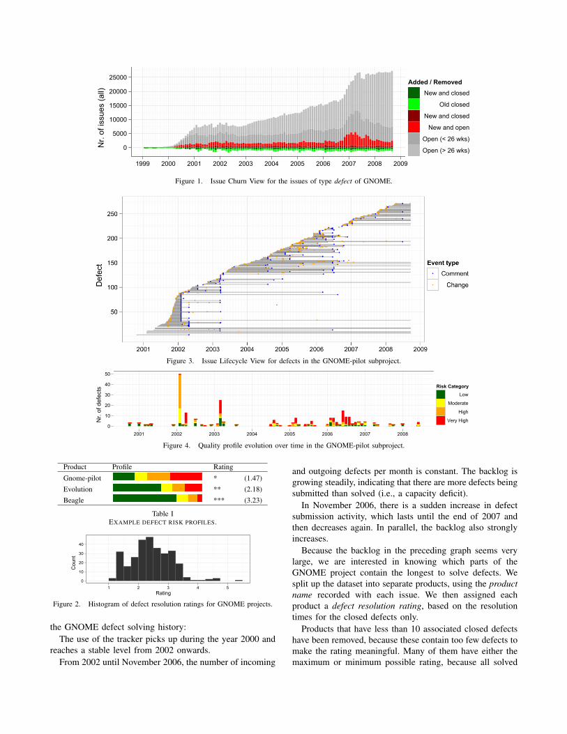
The high-level Issue Churn View (ICV) shows the issuehandling on a monthly basis (see Figure 1). The X-axisrepresents time and the positive and negative values on theY-axis represent, respectively, the number of submitted andresolved issues. For the submitted issues we use (1) darkred to indicate that an issue was opened and solved inthe same month, (2) light red for issues that were openedbut not closed, (3) dark grey for recent backlog (issuesopen ≤ 6 months) and (4) light grey for long-term backlog(issues open > 6 months). For the resolved issues, we againdistinguish between issues both submitted and closed in thismonth (dark green) and older issues that have been solvedin this month (light green).

Important facts that we can derive from the ICV are: thenumber of incoming and outgoing issues, visible throughthe red and green colors, and the development of backlog.An increase of the backlog may indicate that issue solvingcapacity is below what is needed or that submitted bugreports are of low quality and require too much effort toreproduce or track down.

ICVs are best constructed separately for defects and otherissues, since their numbers and priorities are very different.

B. Issue Risk Profiles

To quantify the speed of issue resolution, we aggregateresolution times of individual issues into so-called riskprofiles, which are subsequently mapped to ratings.

We define the resolution time as the time an issue is in anopen state. Thus, we look at the time an issue is marked asbeing in the new or assigned state but not in the closed orresolved state. If an issue has been closed and then reopened,all open intervals count towards the issue resolution time, butthe intervals in which the issue was closed do not.

Individual issue resolution times do not follow a normaldistribution, but rather a power-law-like distribution. As aresult, a simple aggregation by taking the mean or medianof the issue resolution times is not appropriate. Instead weconstruct risk profiles by assigning items to risk categoriesbased on their metric values. For defect resolution time, weuse the following risk categories:

Category ThresholdsLow [0, 28] days (4 weeks)Moderate (28, 70] days (10 weeks)High (70, 182] days (6 months)Very high (182, ∞) days

For example, a defect with a resolution time of 42 daysfalls into the moderate risk category. The thresholds betweenthese risk categories were chosen to coincide roughly withthe 70th, 80th, and 90th percentile of defect resolutiontimes in a set of about 100 releases of various open sourcesoftware products, because at these percentiles the variabilitybetween releases was observed to be higher than at lowerpercentiles [2].

Based on this risk assignment, a risk profile is constructedby calculating the percentage of items in each category.For example, ⟨70, 19, 11, 0⟩ is the risk profile of a producthistory where 70% of all defects were resolved within 4weeks, 89% were solved within 10 weeks, and none tooklonger than 6 months to solve.

Risk profiles can be constructed for the entire history ofa product but also for sub-groups of the defects, such asreleases or sub-products. When grouping issues by productversion, we take the issues that are resolved between thatversion and the next. For grouping by sub-product, weexploit issue categorization tags in the ITS.

Risk profiles can be mapped to ratings to enable straight-forward comparison. We rate on a unitless scale between 0.5and 5.5 that can be rounded to an integral number of stars.By benchmarking against the defect sets of the same 100systems, we calculated the following mapping [2]:

Rating Moderate High Very High***** 8.3% 1.0% 0.0%**** 14% 11% 2.2%*** 35% 19% 13%** 77% 23% 34%

For example, a snapshot with risk profile ⟨70, 19, 11, 0⟩ willbe eligible for a ranking of 3 stars. By interpolation ourranking algorithm establishes an exact rating of 3.25.

Risk profiles and ratings for issue resolution time areuseful for comparing (slices of) the history of softwareproducts in a quantitative manner. As such, systems orcomponents who perform relatively worse can be identifiedand action can be undertaken. Table I shows examples.

C. Issue Lifecycle ViewThe Issue Lifecycle View (ILV), which is loosely based

on the Change History View by Zaidman et al. [3], is ascatter plot of issues versus modification dates. An exampleILV can be seen in Figure 3. The X-axis represents time,while the Y-axis is populated by issues, sorted by the datethey first appeared in the tracker. An issue is represented bya horizontal line fragment, which indicates that the issue ismarked open. Blue dots on this line signify that a commentwas placed on the issue and yellow dots point at otherevents, i.e., any change in a property for that issue, exceptfor opening, closing or commenting (e.g., reassignment,attaching a patch or a change in priority).

A number of interesting facts can be derived from theILV: the number of horizontal lines directly above a point intime (X-axis) shows the number of open issues at that point.The length of the lines indicates the time an issue has beenopen and thus also shows potential backlog. By studyingthe length of lines we also see the age composition of openissues, which in turn helps to understand how the backlog isbeing handled. For example, a system with a constant (non-addressed) backlog has a set of very long lifecycle lines,the backlog, and a set of short lines, issues that are actuallybeing solved. Vice versa, when the backlog is addressed, theline lengths would be more uniform, since the older issuesare solved quicker, but the younger ones slower.

III. INPUT DATA

As input data for the study reported in this paper wehave used and ITS dump of the GNOME project1. This datarepresents the period between 1999-01-01 and 2008-09-19.A few issues from before this period are in the dataset, butwe removed those from our analysis. In the period underanalysis, 431838 issues were recorded. Issues marked asduplicate (143568), invalid (114611, including notgnomeetc.) or wontfix (18093) were not taken into consideration.Using the severity field of each issue, we discovered that22120 of the remaining issues are in fact enhancements andthe rest are true defects (133446). Of these defects, 106932are closed and 26514 are still open.

IV. RESULTS

Figure 1 shows an ICV for the defects in the GNOMEissue tracker. A number of observations can be made about

1http://msr.uwaterloo.ca/msr2009/challenge/gnome data/gnomebugzilla.xml.bz2

Date (month)

Nr.

of is

sues (

all)

0

5000

10000

15000

20000

25000

1999 2000 2001 2002 2003 2004 2005 2006 2007 2008 2009

Added / Removed

New and closed

Old closed

New and closed

New and open

Open (< 26 wks)

Open (> 26 wks)

Figure 1. Issue Churn View for the issues of type defect of GNOME.

Figure 3. Issue Lifecycle View for defects in the GNOME-pilot subproject.

Time

Nr.

of d

efec

ts

0

10

20

30

40

50

2001 2002 2003 2004 2005 2006 2007 2008

Risk Category

Low

Moderate

High

Very High

Figure 4. Quality profile evolution over time in the GNOME-pilot subproject.

Product Profile Rating

Gnome-pilot * (1.47)Evolution ** (2.18)Beagle *** (3.23)

Table IEXAMPLE DEFECT RISK PROFILES.

Rating

Count

0

10

20

30

40

1 2 3 4 5

Figure 2. Histogram of defect resolution ratings for GNOME projects.

the GNOME defect solving history:The use of the tracker picks up during the year 2000 and

reaches a stable level from 2002 onwards.From 2002 until November 2006, the number of incoming

and outgoing defects per month is constant. The backlog isgrowing steadily, indicating that there are more defects beingsubmitted than solved (i.e., a capacity deficit).

In November 2006, there is a sudden increase in defectsubmission activity, which lasts until the end of 2007 andthen decreases again. In parallel, the backlog also stronglyincreases.

Because the backlog in the preceding graph seems verylarge, we are interested in knowing which parts of theGNOME project contain the longest to solve defects. Wesplit up the dataset into separate products, using the productname recorded with each issue. We then assigned eachproduct a defect resolution rating, based on the resolutiontimes for the closed defects only.

Products that have less than 10 associated closed defectshave been removed, because these contain too few defects tomake the rating meaningful. Many of them have either themaximum or minimum possible rating, because all solved

defects are in the highest or lowest risk category. Theresulting dataset contains 300 products. Three example riskprofiles are shown in Table I. For example, Evolution hasthe risk profile ⟨54, 13, 14, 19⟩, giving it a rating of 2.18.

Figure 2 shows a histogram of all ratings for the 300products. The ratings seem to be skewed to the left, in-dicating that in GNOME products it takes longer to solvedefects than in the systems in our calibration set. Lookingat the products in the lower end of this graph, we noticeda number of interesting candidates for further analysis.Gnome-pilot, gnome-media and gnome-core all have morethan 200 defects and a rating below 1.6.

We picked gnome-pilot, a product for hand-held comput-ers, for further investigation. It has 237 closed defects andrates 1.47, with over 35% of defects taking more than half ayear to solve. To find out why this rating is so low, we usethe ILV to investigate the defect lifecycle in more detail.

The ILV for gnome-pilot, Figure 3, shows us that thereare many defects that are open for multiple years. The graphshows a number of clearly visible vertical stripes, where alarge number of defects was solved simultaneously. Lookingat the comments associated to these issues, we found thatmany (but not all) had been solved some time previously,but were left open in the issue tracker. At the dates wherethe stripes show, these were closed as a clean-up.

We suspected these large simultaneous actions to be thecause of the low overall rating. To investigate this, weconstructed an issue resolution quality profile per month forgnome-pilot. The result is displayed in Figure 4. In this graphthe height of a bar indicates how many defects were solved.The peaks coincide with the large actions in the ILV, and areprimarily composed of (very) high risk defects. The largesimultaneous actions do indeed seem to form the bulk ofthe high-risk defects. Nonetheless, since not all defects withlong resolution times are closed as part of clean up actions,the rating of gnome-pilot remains low.

V. RELATED WORK

Kim and Whitehead investigated the bug-fixing time ofeach file in a software system. They found that the files withthe longest bug-fixing time also contain the most bugs [4].Similar to our study, they also try to identify problem areas.

Ihara et al. propose a method to analyze the bug modi-fication process. They calculate the time required to transitbetween states in the bug modification process [5]. Similarto our own study, their aim is to identify bottlenecks in thebug modification process. One of the bottlenecks they haveidentified is the verification of resolved bugs, which was themost time-consuming step in the bug resolution process inboth Apache and Firefox.

VI. CONCLUDING REMARKS

In this paper we have presented three views and anapproach that allow software engineers to retrospectively

assess the issue handling process on the basis of recordedissue data. We have applied these to the GNOME project.We can now answer the research questions of Section I:

RQ1: Can the efficiency of issue handling be assessedin an objective way?: Yes. We can perform a high-levelassessment of the issue handling process using the IssueChurn View. Using Issue Risk Profiles and ratings derivedfrom them, we can zoom in and assess issue handling duringparticular periods and/or for particular system components.Finally, the Issue Lifecycle View allows detailed assessmenton the level of individual issues.

RQ2: Are there significant fluctuations in bug solvingefficiency throughout time?: Yes. In the case of GNOME theIssue Churn View revealed certain periods (e.g., November2006 – end of 2007) with an increase in the number ofdefects reported and a subsequent sharp increase in thedefect backlog. The monthly Issue Risk Profiles showed asimultaneous increase in high risk defects (resolution timesover 6 months) and a drop in the defect resolution rating.

RQ3: Are there significant differences in bug solvingefficiency between software components or packages?: Yes.The Issue Risk Profiles offer a quick way of comparingthe defect solving efficiency, by assigning a rating to eachcomponent. In the case of GNOME we have seen thatthere is a large difference in the time it takes to solvedefects between subprojects, with some packages wheremost defects are solved within 28 days, while for some otherpackages many defects take 182 days or more to solve.

Our case study has shown that a number of straightfor-ward instruments for visualisation and quantification of issuehandling can be used in concert to assess the efficiency ofissue handling both at a high abstraction level and in detail.

In future work we expect to refine these instruments. Inparticular, we want to take into account the difficult to solvea bug (e.g., blocker bugs). Furthermore, we aim to apply ourapproach to commercial software projects.

REFERENCES

[1] J. Anvik, L. Hiew, and G. C. Murphy, “Coping with an openbug repository,” in Proc. 2005 OOPSLA workshop on Eclipsetechnology eXchange (eclipse’05). ACM, 2005, pp. 35–39.

[2] B. Luijten, “The influence of software maintainability on issuehandling,” Master’s thesis, Delft University of Technology,2010.

[3] A. Zaidman, B. Van Rompaey, S. Demeyer, and A. vanDeursen, “Mining software repositories to study co-evolutionof production and test code,” in Proceedings of the Inter-national Conference on Software Testing, Verification andValidation (ICST). IEEE, 2008, pp. 220–229.

[4] S. Kim and E. J. Whitehead, Jr., “How long did it take to fixbugs?” in Proc. Int’l workshop on Mining software repositories(MSR). ACM, 2006, pp. 173–174.

[5] A. Ihara, M. Ohira, and K.-i. Matsumoto, “An analysis methodfor improving a bug modification process in open source soft-ware development,” in Proc. joint int’l workshops on Principlesof software evolution (IWPSE) and software evolution (Evol).ACM, 2009, pp. 135–144.