Exploiting Quality-Efﬁciency Tradeoffs with …homes.cs.washington.edu/~moreau/media/slides/qappa-codes2017-slides...Exploiting Quality-Efﬁciency Tradeoffs with Arbitrary Quantization

Exploiting Quality-Efficiency Tradeoffs with Arbitrary Quantization

Special Session - CODES+ISSS Thierry Moreau, Felipe Augusto, Patrick Howe

Armin Alaghi, Luis Ceze

Internet of Things Revolution

noisy, real world sensory input processing

aggregate analytics,

consumed by human etc.

… double temp = sensor_acquire();

…

… double temp = sensor_acquire();

…

Approximate computing: eliminate inefficiencies in systems by producing just-the-right quality

Quantization: going back to basics

noisy, real world sensory input processing

aggregate analytics,

consumed by human etc.

SRAM

SRAM

ALU

ALU

This Talk: A “Limit Study” on Precision Scaling

n

doublefloat

1

Assumption: hardware that can dynamically and arbitrarily scale its precision

SW Scope: compute heavy, regular applications

HW Scope: hardware accelerators

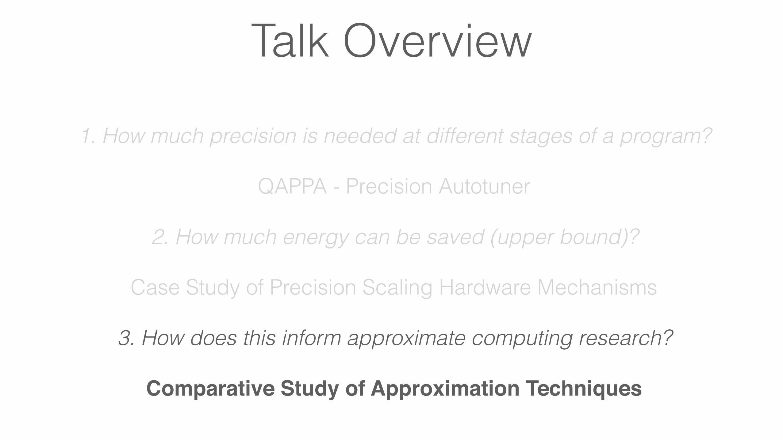
Talk Overview

1. How much precision is needed at different stages of a program?

2. How much energy can be saved (upper bound)?

3. How does this inform approximate computing research?

Talk Overview


QAPPA - Precision Autotuner

2. How much energy can be saved?


QAPPA: Quality Autotuner for Precision-Programmable Accelerators

Goal: Minimize instruction-level precision requirements given a quality target

kernel.c

desired quality target

QAPPA framework instruction-level

precision requirements

quality &energy savings

Built on top of ACCEPT, the approximate C/C++ compiler http://accept.rocks

http://accept.rocks

QAPPA Autotuner Overview

application quality

savings

bad OK

instruction 0instruction 1instruction 2…instruction n-1instruction n

Default (no savings)

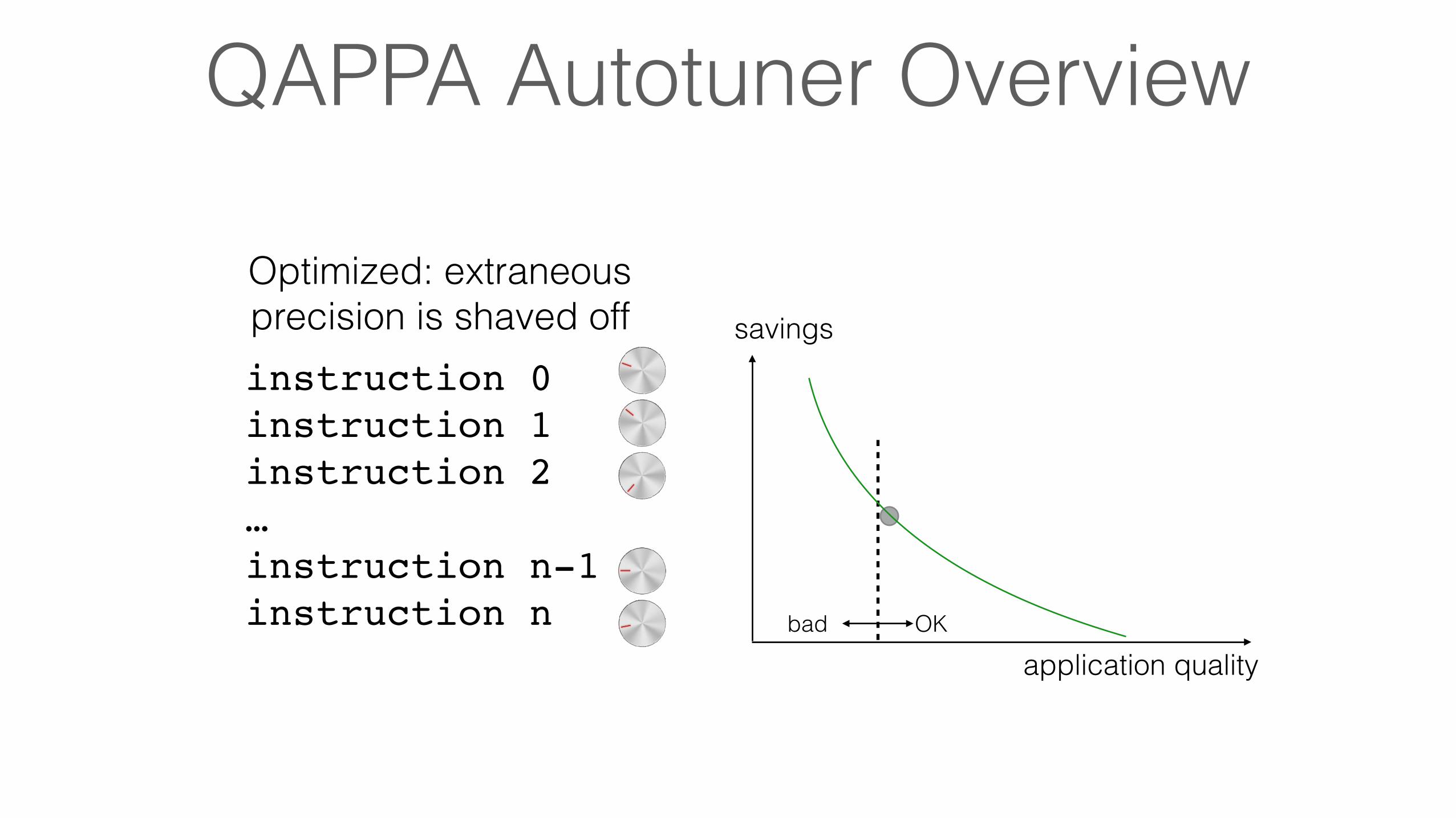
QAPPA Autotuner Overview

instruction 0instruction 1instruction 2…instruction n-1instruction n

Optimized: extraneous precision is shaved off savings

bad OK

application quality

QAPPA 5-Step Description

AnnotatedProgram

Program Inputs &Quality Metrics

ACCEPTstatic analysis ILPC*

ACCEPTerror injection & instrumentation

ApproximateBinary

Execution & Quality

Assessment

Quality AutotunerOutput Configuration

Quality Results& Bit Savings

* Instruction-level Precision Configuration

1. Program AnnotationAnnotatedProgram




ApproximateBinary

Execution & Quality

Assessment




void conv2d (APPROX pix *in, APPROX pix *out, APPROX flt *filter){ for (row) { for (col) { APPROX flt sum = 0 int dstPos = … for (row_offset) { for (col_offset) { int srcPos = … int fltPos = … sum += in[srcPos] * filter[fltPos] } } out[dstPos] = sum / normFactor } }}

Key: use the APPROXtype qualifier [*]

[*] EnerJ, Sampson et al., PLDI’11

2. Static Analysis

Instruction-Level Precision Configuration (ILPC)

conv2d:13:7:load:Int32 conv2d:13:10:load:Float conv2d:13:11:fmul:Float conv2d:13:12:fadd:Float conv2d:15:1:fdiv:Float conv2d:15:7:store:Int32

void conv2d (APPROX pix *in, APPROX pix *out, APPROX flt *filter){ for (row) { for (col) { APPROX flt sum = 0 int dstPos = … for (row_offset) { for (col_offset) { int srcPos = … int fltPos = … sum += in[srcPos] * filter[fltPos] } } out[dstPos] = sum / normFactor } }}

ACCEPT

AnnotatedProgram




ApproximateBinary

Execution & Quality

Assessment




ACCEPT identifies safe-to-approximate instructions from data annotations using flow analysis

3. Error InjectionAnnotatedProgram




ApproximateBinary

Execution & Quality

Assessment




Approximate Binary

Instruction-Level Precision Configuration (ILPC)

conv2d:13:7:load:Int4 conv2d:13:10:load:Fix2.3 conv2d:13:11:fmul:Fix2.3 conv2d:13:12:fadd:Fix4.5 conv2d:15:1:fdiv:Fix2.3 conv2d:15:7:store:Int4

Instrumentation & Compilation

Each instruction in the ILCP acts as a quality knob that the autotuner can use to maximize bit-savings

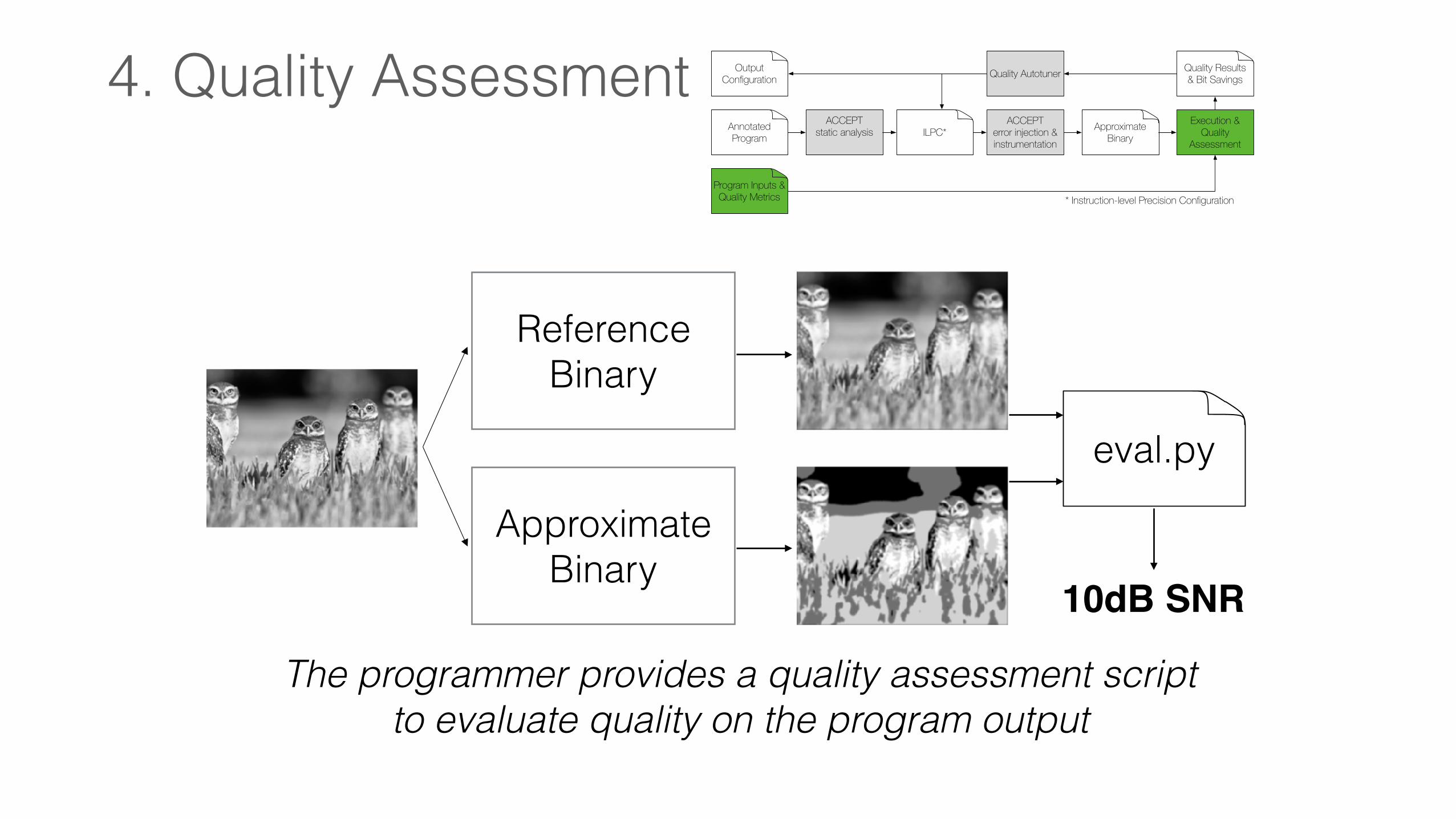
4. Quality AssessmentAnnotatedProgram




ApproximateBinary

Execution & Quality

Assessment




The programmer provides a quality assessment script to evaluate quality on the program output

Reference Binary

Approximate Binary

eval.py

10dB SNR

5. Autotuning AlgorithmAnnotatedProgram




ApproximateBinary

Execution & Quality

Assessment




config k: error = 0.10%

config [k+1, i-1]: error = 5.91%

config [k+1, i]: error = 0.30%

config [k+1, i+1]: error = 0.12%

config [k+2, i-1]: error = 5.91%

config [k+2, i]: error = 0.33%

config [k+2, i+1]: error = 1.6%

…

…

…

…

…

…

Greedy iterative algorithm [*]: reduces precision requirement of the instruction that impacts quality the least

Finds solution in O(m2n) worst case where m is the number of static safe-to-approximate instructions and n are the levels of precision for all instructions

[*] Precimonious, Rubio-Gonzalez et al., SC’13

AnnotatedProgram




ApproximateBinary

Execution & Quality

Assessment




precise60dB40dB

20dB

10dB The autotuner greedily maximizes bit-savings as the quality target is lowered

5. Autotuning Algorithm

PERFECT Application StudyApplication Domain Kernels Metric

PERFECT Application 1Discrete Wavelet Transform

Signal to Noise Ratio(SNR)

[120dB to 10dB] (0.0001% to 31.6% MSE)

2D ConvolutionHistogram Equalization

Space Time Adaptive Processing

Outer ProductSystem SolveInner Product

Synthetic Aperture RadarInterpolation 1Interpolation 2

Back Projection

Wide Area Motion ImagingDebayer

Image RegistrationChange Detection

Required Kernels FFT 1DFFT 2D

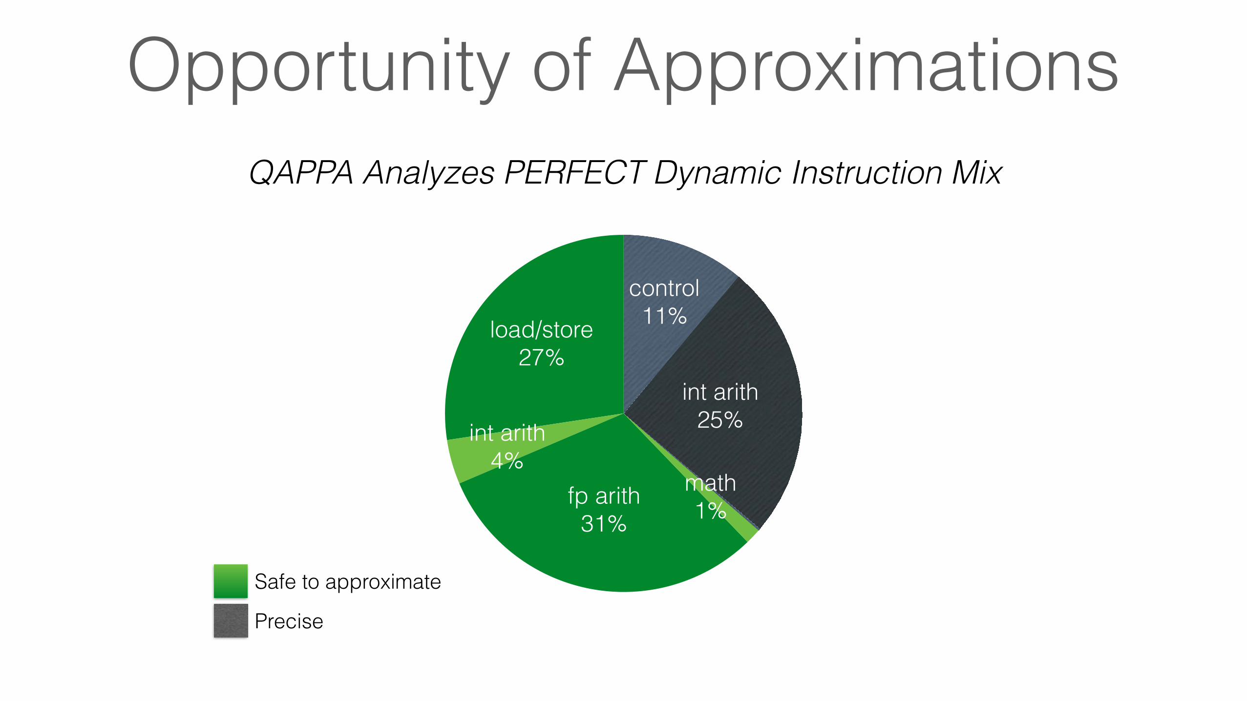
Opportunity of ApproximationsQAPPA Analyzes PERFECT Dynamic Instruction Mix

load/store27%

int arith4%

fp arith31%

math1%

int arith25%

control11%

Safe to approximate

Precise

Average Precision Reduction Achieved Across PERFECT Kernels

Dyn

amic

pre

cisi

on re

duct

ion

on

safe

-to-a

ppro

xim

ate

inst

ruct

ions

0%

20%

40%

60%

80%

100%

Target Application SNR (dB)10 20 40 60 80 100 120

26%32%

40%48%

57%

74%

83%

High QualityApproximateMore savings


Dyn

amic

pre

cisi

on re

duct

ion

on

safe

-to-a

ppro

xim

ate

inst

ruct

ions

0%

20%

40%

60%

80%

100%

Average SNR (dB)10 20 40 60 80 100 120

26%32%

40%48%

57%

74%

83%

PERFECT Manual 0.001% MSE


Dyn

amic

pre

cisi

on re

duct

ion

on

safe

-to-a

ppro

xim

ate

inst

ruct

ions

0%

20%

40%

60%

80%

100%

Average SNR (dB)10 20 40 60 80 100 120

26%32%

40%48%

57%

74%

83%

Approximate Computing 10% MSE

Talk Overview




Case Study of Precision Scaling Hardware Mechanisms


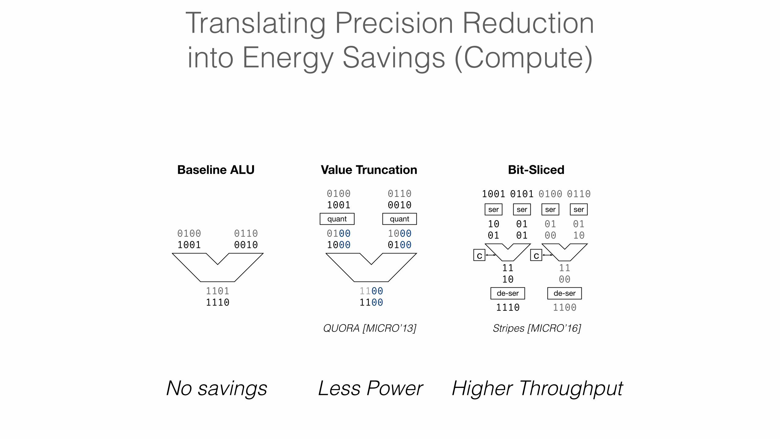
Translating Precision Reduction into Energy Savings (Compute)

11011110

01001001

01100010

(a) (b)

01001000

11001100

10000100

quant quant

01001001

01100010

(c)

1001

1110

0101

c

ser ser1001 0101

de-ser

1110

0100

1100

0110

c

ser ser0100 0110

de-ser

1100

(d)

10

11

01

c

q q1001 0101

de-ser

1100

01

11

10

c

q q0100 0110

de-ser

1100

Baseline ALU

No savings


11011110

01001001

01100010

(a) (b)

01001000

11001100

10000100

quant quant

01001001

01100010

(c)

1001

1110

0101

c

ser ser1001 0101

de-ser

1110

0100

1100

0110

c

ser ser0100 0110

de-ser

1100

(d)

10

11

01

c

q q1001 0101

de-ser

1100

01

11

10

c

q q0100 0110

de-ser

1100

QUORA [MICRO’13]

Baseline ALU Value Truncation

No savings Less Power


11011110

01001001

01100010

(a) (b)

01001000

11001100

10000100

quant quant

01001001

01100010

(c)

1001

1110

0101

c

ser ser1001 0101

de-ser

1110

0100

1100

0110

c

ser ser0100 0110

de-ser

1100

(d)

10

11

01

c

q q1001 0101

de-ser

1100

01

11

10

c

q q0100 0110

de-ser

1100

Bit-Sliced

Stripes [MICRO’16]QUORA [MICRO’13]

Baseline ALU Value Truncation

No savings Less Power Higher Throughput

Case Study: Precision Scaled Adder

Methodology: Post-place-and-route prime-time power analysis on 65nm TSMC library

Goal: Design an precision scalable adder that can elegantly trade lower precision for energy savings

Exploration: Combine value truncation and bit slicing techniques, and vary the slice width in increments of powers of 2

Precision Scaled Adder Study

Ener

gy C

ost (

pJ)

0.00

0.45

0.90

1.35

1.80

Input Bit-Width

0 8 16 24 32 40 48 56 64

64

technique 1: value truncation

offset due to static power

Precision Scaled Adder Study

Ener

gy C

ost (

pJ)

0.00

0.45

0.90

1.35

1.80

Input Bit-Width

0 8 16 24 32 40 48 56 64

1 64

technique 2: bit slicing

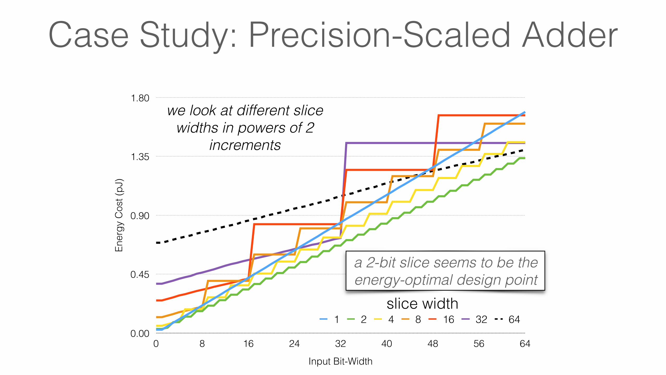
Case Study: Precision-Scaled Adder

Ener

gy C

ost (

pJ)

0.00

0.45

0.90

1.35

1.80

Input Bit-Width

0 8 16 24 32 40 48 56 64

1 2 4 8 16 32 64

we look at different slice widths in powers of 2

increments

slice width

a 2-bit slice seems to be the energy-optimal design point

Average Compute Energy Savings vs. Application SNREn

ergy

Sav

ings

(x) -

Hig

her i

s Be

tter

0

1

2

3

4

5

6

7

8

9

10

Application SNR (dB) - Higher is Better

20 30 40 50 60

2.52.62.93.13.8 3.6

4.34.8

5.6

7.1

2.83.03.23.6

7.7

1.41.51.72.02.5

1 2 4 816 32

PERFECT Study: Compute Energy Savings

quora

stripesslice width



ergy

Sav

ings

(x) -

Hig

her i

s Be

tter

0

1

2

3

4

5

6

7

8

9

10


20 30 40 50 60

2.52.62.93.13.8 3.6

4.34.8

5.6

7.1

2.83.03.23.6

7.7

1.41.51.72.02.5

1 2 4 816 32

slice widthAt 40dB a 16b sliced ALU can

achieve 4.8 energy reduction!



ergy

Sav

ings

(x) -

Hig

her i

s Be

tter

0

1

2

3

4

5

6

7

8

9

10


20 30 40 50 60

2.52.62.93.13.8 3.6

4.34.8

5.6

7.1

2.83.03.23.6

7.7

1.41.51.72.02.5

1 2 4 816 32

slice widthAt 20dB the optimal design

point shifts to 8-bit slice

Talk Overview






Comparative Study of Approximation Techniques

Comparative StudyMany papers on approximate computing state:

“Our technique provided n times speedup at x% error”

Problem: This give us a data point but doesn’t quite say much about the merits of the technique at

trading accuracy for efficiency

Solution: Use QAPPA to produce quick comparison results to assess effectiveness of technique

Comparative Study - Voltage Overscaling

0

10

0.8

20

01

Erro

r Pro

babi

lity

(%)

2

30

30.85 456

40

789100.9 11

Overscaling Factor

1213

Bit Position

141516170.95 181920212223241 25262728293031

Methodology (1/2): Spice simulation of ALU/FPU design under different voltage overscaling factors.

fp adder example

Comparative Study - Voltage Overscaling

Results: Precision scaling always produces better quality/efficiency

Methodology (2/2): Then we feed the error model into QAPPA’s error injection framework to assess

application error.SN

R (d

B) -

hige

r is

bette

r

0

10

20

30

40

2dconv

dwthisteq

outersystemsolve

innerinterp1

interp2bp debayer

lucaskanade

changedet

fft1dfft2d

VOF=0.95 VOF=0.90 VOF=0.84

Future Directions in Architecture/CAD

Precision Scaling Architectures: Need to see more precision-scaled accelerators for more applications of the likes of Quora[MICRO’13], Stripes[MICRO’16]

CAD tools with Quality Awareness: Need to see more tools that can leverage quantization, especially in the

FPGA community, of the likes of AHLS[DATE’17]

Conclusion






Comparative Study of Approximation Techniques

Special Session - CODES+ISSS Thierry Moreau, Felipe Augusto, Patrick Howe

Armin Alaghi, Luis Ceze

Exploiting Quality-Efficiency Tradeoffs with Arbitrary Quantization

Thank you!

Documents

Exploiting Quality-Efﬁciency Tradeoffs with …homes.cs.washington.edu/~moreau/media/slides/qappa-codes2017-slides...Exploiting Quality-Efﬁciency Tradeoffs with Arbitrary Quantization