ORCA-Quest qCMOS camera C15550-20UP Technical note

Technical noteSEP 2021

ORCA®-QuestqCMOS® camera C15550-20UP

2

Table of contents

Introduction ······································· P3

1. Key Features ································· P31-1. Readout noise1-2. Photon number resolving

2. Sensor Features ···························· P72-1. Sensor readout structure2-2. Back illuminated sensor2-3. Deep trench isolation structure2-4. On-chip micro lens2-5. Quantumefficiency2-6. MTF (Modulation Transfer Function)2-7. Etaloning-desensitized2-8. Sensor size2-9. Digitization2-10. Simultaneous dual-row readout with

single direction

3. Camera Features ························· P103-1. Readout and frame rate3-2. Camera structure and features

4. Readout Modes ··························· P124-1. Readout modes4-2. Scan modes4-3. Operation modes4-4. Other readout modes

5. Synchronization ·························· P145-1. Synchronizationwithotherinstruments5-2. Trigger input5-3. Trigger output5-4. Master pulse

6. Data Managements ······················ P166-1. Selectable pixel bit depth6-2. User selectable Look Up Table (LUT)6-3. Real-time defect pixel correction6-4. PhotoResponseNon-Uniformity(PRNU)

andDarkSignalNon-Uniformity(DSNU)

7. Software Support ························· P177-1. DCAM-API®

7-2. DCAM-SDK & DCIMG-SDK7-3. Hamamatsu software7-4. Thirdpartysoftwaresupport/options

8. Various Timing Charts ·················· P188-1. Explanation of timing charts8-2. Standard and Ultra quiet scan mode8-3. Normal area and photon number

resolving modes8-4. Lightsheet readout mode

9. Understanding SNR ····················· P229-1. SNR9-2. rSNR9-3. Camera Simulation Engine

10. Application Examples ·················· P2310-1.Quantumtechnology

(Neutral atom, Ion trap)10-2.Astronomy(Lucky/Speckleimaging)10-3. Life science

(Delayedfluorescenceofplants)10-4.Ramanspectroscopy

11.Specifications ····························· P2511-1.Specificationchart11-2. Dimensional Outlines11-3.SystemConfiguration11-4. Options

1.KeyFeatures

3

1. Key Features

1-1. Readout noise1-1-1. Readout noiseFundamentally,acamerahasthreetofourtypesnoisesources:readout noise, dark current noise, photon shot noise and in the caseofelectronmultiplyingcameras,excessnoise. (Refer tothe white paper “ORCA®-Flash4.0 Changing the Game”, https://www.hamamatsu.com/resources/pdf/sys/e_flash4_whitepaper.pdf). The excess noise is a unique to EM-CCDs, and is not present in CCD and CMOS cameras. In the absence of excess noise, the readout noise becomes the noise which determines the low light performance of the camera. Especially forqCMOS®, the readout noise is the most important as photon number resolving capability can only be performed withextremelylowreadoutnoise.The dominant factor of readout noise is the noise generated at the floating diffusion amplifier (FDA) of the sensor. TheqCMOS® is designed to minimize the readout noise using cutting edge technology. Not only in optimizing the FDAbut also the correlated double sampling (CDS) and other electronics, give the ORCA®-Quest the lowest readout noise which has never been seen before.

1-1-2. Readout noise measurement methodSincetheCCDimagesensorhasonereadoutamplifierpersensor, the readout noise of multiple pixels in a single image can be utilized to measure the read noise.In contrast, as the CMOS image sensor has an amplifierforeachpixel, the readoutnoise isdifferent foreachpixel.Therefore, the readout noise in each pixel (called pixel readout noise)mustbemeasuredfromhundredsofimagesfirst.Themedianandrootmeansquare(rms)noisesarestatisticallycalculated from the distribution of those pixel readout noises.In CMOS cameras of other manufacturers, Median readout noises are used for camera readout noises. Since the median ignores the shape of the distribution of readout noise presentinCMOScameras,especiallyforsCMOScameras,the RMS is used for the metric which includes the shape of the distribution recently. Together, both metrics providean estimate for the noise distribution across the sensor, which can be seen in Fig. 1-1. In some sCMOS cameras themediansaresignificantlylowerthanRMS,thereforeitisimportanttocomparecamerasbythesamemetric.

Introduction

The ORCA®-QuestisthefirstquantitativeCMOS(qCMOS®) camera which has photon number resolving capability.Photonnumberresolving isuniqueandquitedifferent fromphoton counting (more precisely the method resolves thenumber of photoelectrons. However, since single photon counting instead of single photoelectron counting has been usedasacomparablemethod in thisfield,wewilluse theterm “photon number resolving” in this technical note).Photon counting is well-known as a quantitative method of measurement because it can mitigate the readout noise (electronic circuit noise) and multiplication noise (excess noise). It is often used with photomultiplier tubes (PMT) and 2D sensors such as EM-CCD and Intensified CCDcameras.They all have the electronmultiplication functionwhichenablesphotoncountingandtheabilitytodistinguishbetween zero or one photon. However they cannot countmultiple photon numbers like one, two, three, etc., because the electron multiplication function generates noise which detrimentallyeffectstheabilitytocountmultiplephotons.The ORCA®-Quest has extremely low readout noise andcan therefore realize photon counting. Since the ORCA®-Quest can achieve photon counting without an electron multiplication function, it can also count multiple photons (This is called “Photon number resolving”). This photon number resolving method enables accurate and quantitative measurements in a wider range of photons than a standard photon counting method. Additionally, the ORCA®-Quest hasnotonlyphotonnumberresolvingbutalsoalargepixelnumber of 9.4 megapixels. It is much larger than the EM-CCD’s pixel number of 1 megapixel. (Refer to Hamamatsu’s white paper, “qCMOS®: Quantitative CMOS technologyenabledbyPhotonNumberResolving”).The ORCA®-Quest has a lot of unique features ideal for a wide range of imaging applications in addition to photon number resolving, and we will introduce them in this technical note.

qCMOS® sensors

https://www.hamamatsu.com/resources/pdf/sys/e_flash4_whitepaper.pdf

1.KeyFeatures

4

1-1-3. Readout noise performanceFig. 1-1 shows typical pixel readout noise distributionsof qCMOS® (in red), Gen III sCMOS (in green) and Gen II sCMOS (in blue). It clearly shows that distribution shapesare different for each sensor. The distribution of qCMOS® has the lowest peak, the narrowest FWHM and a short thin tail. The distribution of Gen III sCMOS has the second lowest peak, the second narrowest FWHM and a short thick tail. The distribution of Gen II sCMOS has the highest peak, the widest FWHM and a long thick tail.The anti-symmetrical shape of the distribution results in awide variation of statistical readout noise values. The RMS readout noises of qCMOS® is 0.27 electrons, mean readout noise is 0.24 electrons, median readout noise is 0.21 electrons andmodereadoutnoiseis0.19electrons.Theyshowahalfof pixel readout noises are less than 0.21 electrons and peak pixel readout noise is 0.19 electrons.

Readout noise (electrons)

qCMOS®

Gen III sCMOSGen II sCMOS

10-4

10-3

10-2

10-1

1

Rel

ativ

e fre

quen

cy

0 2 4 6 8 10

Fig. 1-1. Typicalpixelreadoutnoisedistributions

1-1-4. Cumulative pixel number ratio for readout noises

Fig. 1-2 shows typical cumulative pixel number ratio forreadout noises of qCMOS®. It shows 95.5 % of pixels are less than 0.40 electrons rms, 82.5 % are less than 0.3 electrons and 75.1 % are less than 0.27 electrons rms.

0.000

0.100

0.200

0.300

0.400

0.500

0.600

0.700

0.800

0.900

1.000

0 0.1 0.2 0.3 0.4 0.5 0.6 0.7 0.8 0.9 1

Cum

ulat

ive

ratio


Fig. 1-2. Typicalcumulativepixelnumberratioforreadout noises of qCMOS®

1-2. Photon number resolving1-2-1. Photon number resolvingAs mentioned, photon number resolving is quite differentfrom photon counting. Photon counting cameras which use multiplication gain such as EM-CCDs or ICCDs to accomplish the low noise needed for counting photons can never realize photon number resolving because of their excess multiplicationnoise.Onthecontrary,qCMOS® achieves the low noise for photon counting without the multiplication gain, and therefore without the multiplication noise.Fig. 1-3 shows the probability distribution of the observedphotoelectrons for a Poisson distribution P3(k) with a mean of N = 3 photoelectrons, and three different values of thereadout noise: σR = 0.5 electrons rms (blue curve), σR =0.3electronsrms(redcurve),andσR=0.15electronsrms(green curve). The smaller the readout noise is the deeper thevalleysbetween thephotoelectronpeaks. If theCMOSsensor can reduce the readout noise, it enables photon number resolving.

Normalized photodetection signal (electrons)

Prob

abilit

y de

nsity

0.7

0.6

0.5

0.4

0.3

0.2

0.1

0.00 1 2 3 4 5 6 7 8

Fig. 1-3. Probabilitydistributionoftheobservedphotoelectronsfor a Poissonian distribution P3(k) with a mean of N=3 photoelectrons,andthreedifferentvaluesofthereadoutnoise:σR=0.5electrons(bluecurve),σR=0.3electrons(redcurve),andσR=0.15electrons(greencurve).

The following graph is real qCMOS® data measured with a single pixel and hundreds of frames. The readout noise of the pixel is 0.16 electrons. The average generated photoelectron number is 2 electrons. The real distribution at approx. 2 electrons seems almost the same as the simulated distribution.

Frame number

Out

put V

alue

(D

igita

l Num

ber)

Out

put V

alue

(D

igita

l Num

ber)

200

190

180

170

150

160

140

1300 800200 400 600 1000

Frequency

0 800200 400 600 1000

6 photons

5 photons

4 photons

2 photons

3 photons

1 photon

0 photon

Threshold200

190

180

170

150

160

140

130

Fig. 1-4. Averagegeneratedphotoelectronnumber:approx.2electrons,Readoutnoise:0.16electrons

1.KeyFeatures

5

The following graph is also real qCMOS® data measured with a single pixel, the readout noise of which is 0.16 electrons. The average generated photoelectron number is 55 electrons. Even with a large photoelectron number, the distribution can showthevalleysclearly.

Frame number

Out

put V

alue

(D

igita

l Num

ber)

Out

put V

alue

(D

igita

l Num

ber)

680660640620600

560580

540

500520

0 800200 400 600 1000

700680660640620600

560580

540

500520

Frequency0 8020 40 60 100 120 140 160 180

700

Fig. 1-5. Averagegeneratedphotoelectronnumber: 55electrons,Readoutnoise:0.16electrons

1-2-2. Error rateThe error rate is the percent probability that each datasamplecanbeclassifiedasanincorrectphotonnumber,orfalsedata.Asthiserrorrateincreases,thevalleysbetweenthe photoelectron peaks become shallower and the photon number becomesmore difficult to resolve. This probabilitythatthedatasamplewillbeclassifiedasthenexthigher,ornext lower photoelectron number is dependent the sample distribution caused by the readout noise. Tomake photonnumberresolvingpossiblethereshouldbeahighprobabilitythat the data sample will be within ±0.5 electrons of the nominalnumber.Conversely, thismeansthat theerrorrateneeds be low that the data sample will fall outside of this range.Fig. 1-6 shows the -0.5 electrons to +0.5 electrons error rates vs readout noise for a range of readout noises to include those shown in Fig. 1-3. From this curve it can be noted that for a readout noise of 0.5 electrons rms, then 31.7 % of the data samples will be false. If the readout noise is 0.25 electrons rms, then 4.6 % of the data samples will be false, and if the readout noise is 0.167 electrons rms, then 0.3 % of the data samples will be false.

10-1

10-2

10-3

10-4

10-5

1

0.10 0.15 0.20 0.25 0.30 0.35 0.40 0.45 0.50 0.55

Sigma (electrons)

Nor

mal

ized

are

a ou

tsid

e [-0

.5, 0

.5]

Fig. 1-6. Error rates vs readout noise

1-2-3. Readout noise at photon number resolving

Photon number resolving (PNR) is a method that converts output signals of the electron number from real number to an integral number. As we can estimate from Fig. 1-3, the numbers after the decimal point aremade by the readoutnoise.Ifthereadoutnoiseisverysmall,thenumbersafterthedecimalpointcanberemovedbythePNRmethod.Onthecontrary, if thereadoutnoise isnotsmall, then thereadoutnoise is detected in its error rates.Fig. 1-7 shows simulated readout noise when it is measured with the PNR method. If the original readout noise is less than 0.3 electrons, then the readout noise with PNR method is smaller than original. If the original readout noise are 0.2 electrons, the readout noise with the PNR method become approximately 0.1 electrons. If the original readout noiseis 0.1 electrons, the readout noise with the PNR method becomesapproximately0electron.

0.0

0.2

0.4

0.6

0.8

1.0

0.0 0.2 0.4 0.6 0.8 1.0

Rea

dout

noi

se w

ith P

hoto

n nu

mbe

r re

solv

ing

(ele

ctro

ns)


Photon number resolvingOriginal

Fig. 1-7. Readout noise at photon number resolving

1-2-4. Photon number resolving modeThe ORCA®-Quest has a photon number resolving mode whichcanoutputtheelectronnumberbyadaptingthephotonnumber resolving method inside the camera. When the photon number resolving mode is selected, the scan speed is set to Ultra quiet scan mode and one count of output data becomesoneelectron.Thesensorpixelgainsaredifferentin pixel by pixel, but the photon number resolving modecan output themore precise photon number by correctingpixelgaindifferencesinsidethecamera.Asphotonnumberresolvingisvalidtoonlyahighgainamplifierwithlownoise,the maximum output of photon number resolving mode becomes 200 counts which is equivalent to 200 electrons.

1.KeyFeatures

6

1-2-5. Merit of photon number resolving mode

The merit of photon number resolving mode is that it has a wider detectable photon number range when compared to traditional photon counting cameras. It has the potential to providesuperiormeasurementinlinearity.With the photon counting camera, the input photon number for each pixel must be less than one pixel/frame to keepgoodlinearity.However,itisverydifficultforphotoncountingcameras to keep less than one electron/pixel/frame on allpixels because it can output just zero or one electron. The users try to estimate whether all pixels are less than oneelectron/pixel/frameornotbycalculatingthemeanofsomeframes.Ifnot,theymustreducetheinputphotonnumbertolessthanoneelectron/pixel/framebyanymeansorgiveupthemeasurementwithgoodlinearity.With the photon number resolving mode of the ORCA®-Quest, the camera outputs photon numbers and it can be usedatsignallevellessthan200electrons/pixel/framewhilekeepinggoodlinearity.Thephotonnumberresolvingmodeisveryusefulforpreciseimaging when there are both high and low photon number regions.

1-2-6. Binning in photon number resolving mode

As described in section “4-4-2 Binning readout”, the binning is a method of adding the signal of adjacent pixels together to achievehighsensitivityatthecostofresolution.Thisbinningfor CMOS sensors which is called digital binning, adds not only signals but also readout noises. However, ORCA®-Quest’sreadoutnoiseisverysmallevenwhenincreasedbybinning.Additionally,asFig.1-7shows,readoutnoiseswiththe PNR method become smaller than the original readout noises.In terms of binning and PNR method, we have two alternatives, thefirst isperforming thePNRmethodbeforebinning,andthe second is performing binning before PNR method. Since the PNR method has higher merit for low readout noise, the ORCA®-Quest performs the PNR method before increasing thereadoutnoisebybinning.

2. Sensor Features

7

2. Sensor Features

2-1. Sensor readout structureThefollowingfigure is thereadoutstructureof theORCA®-Quest qCMOS® sensor very similar to standard sCMOSsensor. Each pixel has a photodiode (PD) and Floating DiffusionAmplifier(FDA).AtthePDthephotonsareconvertedto photoelectrons and at the FDA the photoelectrons are converted to voltages. The FDA is the dominant source of readout noise of the sensor. Each column has two Correlated Double Samplings (CDSs) and column Analog to Digital Converters (ADCs). Even and odd rows are readout simultaneously fromtop tobottom.EvenandoddrowsarereadoutthroughdifferentCDSsandADCs.

Fig. 2-1. Sensor structure

2-2. Back illuminated sensorThe ORCA®-Quest qCMOS® sensor has a cutting edge back illuminatedsensorwhichhasnotonlyhighQE,butalsohighresolution.

2-3. Deep trench isolation structureThe ORCA®-Quest features a deep trench pixel structure, an innovationinscientificimagesensors.Thebackilluminatedsensor is thinned to less than 20μm thickness to achievehigher resolution in short and visible wavelengths. For a sensorwithasmallpixelsize,athinnersensorisnecessaryforgoodresolution.Onthecontrary, thinnersensorscausethe lower quantum efficiency in near infra-red wavelength(NIR).Sothereisatrade-offbetweenresolutionandquantumefficiencydependingonthesensorthickness.The ORCA®-Quest has a sensor which has enough thickness for NIR-QE with a deep trench structure in each pixel, and it enables both good resolution and NIR-QE with the small sensorsizeof4.6μmsquareeven.Thetrenchstructurecanreflecttheinputphotonsandpreventthemfromreachingtheadjacent pixels. It prevents not only the input photons, butalso the photoelectrons from migrating to the adjacent pixels.

1

2

3

5

4

Fig. 2-2. Schematic cross section through the back-illuminated qCMOS® image sensor showing DTI (Deep Trench

Isolation) structures and microlenses on top.1:Microlenses,2:Field-freeregion(photochargetransportthroughdiffusion),3:DTI(DeepTrench

Isolation)structures,4:Electricfieldregion(photochargetransportthroughdrift),5:Pixelstructure

for electronic photocharge detection

2-4. On-chip micro lensThe ORCA®-Quest has an on-chip micro lens in each pixel. The microlenses compensate for the loss in active area due to the DTI structures and therefore maximize QE.

2. Sensor Features

8

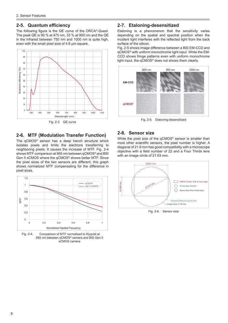
2-5. QuantumefficiencyThe following figure is theQE curve of theORCA®-Quest. The peak QE is 90 % at 475 nm, 33 % at 900 nm and the QE in the infrared between 750 nm and 1000 nm is quite high, evenwiththesmallpixelsizeof4.6μmsquare.

0

10

20

30

40

50

60

70

80

90

100

Qua

ntum

effi

cien

cy (%

)

300 400 500 600 700 800 900 1000 1100

Wavelength (nm)

Fig. 2-3. QE curve

2-6. MTF (Modulation Transfer Function)The qCMOS® sensor has a deep trench structure which isolates pixels and limits the electrons transferring to neighboring pixels. It causes the increase of MTF. Fig. 2-4 shows MTF comparison at 565 nm between qCMOS® and BSI Gen II sCMOS where the qCMOS® shows better MTF. Since the pixel sizes of the two sensors are different, this graphshows normalizedMTF compensating for the difference inpixel sizes.

Normalized Spatial Frequency

MTF

10.80.60.40 0.2

1

0.8

0.6

0.4

0

0.2

1.2

qCMOS®

Gen II sCMOS

Fig. 2-4. ComparisonofMTFnormalizedtoNyquistat565 nm between qCMOS® camera and BSI Gen II

sCMOS camera

2-7. Etaloning-desensitizedEtaloning is a phenomenon that the sensitivity variesdepending on the spatial and spectral position when the incidentlightinterfereswiththereflectedlightfromthebacksurface of the silicon.Fig.2-5showsimagedifferencebetweenaBSIEM-CCDandqCMOS® with uniform monochrome light input. While the EM-CCD shows fringe patterns even with uniform monochrome light input, the qCMOS®doesnotshowsthemclearly.

EM-CCD

qCMOS®

800 nm 900 nm 1000 nm

Fig. 2-5. Etaloning-desensitized

2-8. Sensor sizeWhile the pixel size of the qCMOS® sensor is smaller than mostotherscientificsensors, thepixelnumber ishigher.Adiagonalof21.6mmhasgoodcompatibilitywithamicroscopeobjectivewithafieldnumberof22andaFourThirds lenswith an image circle of 21.63 mm.

18.841 mm

21.617 mm

10.5

98 m

m ORCA®-Quest: field of view angle

Microscope Adapter

Macro lens (Four thirds lens)

Number of field of view 22 mmImage circle 21.63 mm

Fig. 2-6. Sensor size

2. Sensor Features

9

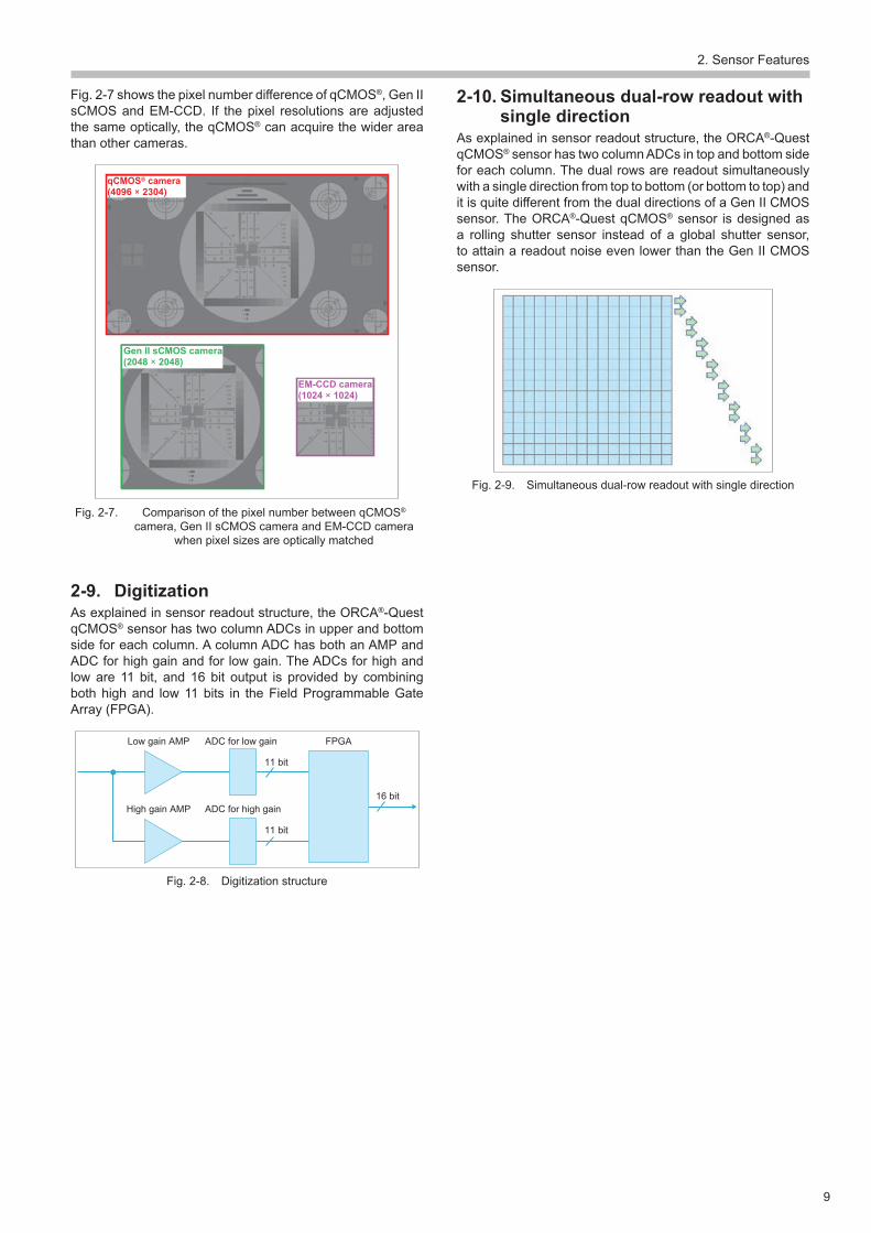
Fig.2-7showsthepixelnumberdifferenceofqCMOS®, Gen II sCMOS and EM-CCD. If the pixel resolutions are adjusted thesameoptically,theqCMOS® can acquire the wider area than other cameras.

qCMOS® camera (4096 × 2304)

Gen II sCMOS camera (2048 × 2048)

EM-CCD camera(1024 × 1024)

Fig. 2-7. Comparison of the pixel number between qCMOS® camera, Gen II sCMOS camera and EM-CCD camera

whenpixelsizesareopticallymatched

2-9. DigitizationAs explained in sensor readout structure, the ORCA®-Quest qCMOS® sensor has two column ADCs in upper and bottom side for each column. A column ADC has both an AMP and ADC for high gain and for low gain. The ADCs for high and low are 11 bit, and 16 bit output is provided by combiningboth high and low 11 bits in the Field Programmable Gate Array(FPGA).

Low gain AMP

High gain AMP ADC for high gain

ADC for low gain FPGA

11 bit

11 bit

16 bit

Fig. 2-8. Digitization structure

2-10. Simultaneous dual-row readout with single direction

As explained in sensor readout structure, the ORCA®-Quest qCMOS® sensor has two column ADCs in top and bottom side foreachcolumn.Thedualrowsarereadoutsimultaneouslywith a single direction from top to bottom (or bottom to top) and itisquitedifferentfromthedualdirectionsofaGenIICMOSsensor. The ORCA®-Quest qCMOS® sensor is designed as a rolling shutter sensor instead of a global shutter sensor, to attain a readout noise even lower than the Gen II CMOS sensor.

Fig. 2-9. Simultaneous dual-row readout with single direction

3. Camera Features

10

3. Camera Features

3-1. Readout and frame rate3-1-1. Frame rate (readout speed)The frame rate (readout speed) refers to the number of imagesthatcanbecontinuouslyproducedandisspecifiedinframes per second (fps). The maximum full frame rate of the ORCA®-Questis120frames/s(at4096×2304pixels)andisachieved using a simultaneous dual-row readout with single direction.

0.46

0.89

1

Relative S/R ratio(Wavelength 500 nm, 1 photon/pixel)

Number of pixels(megapixel)

Data rate(megapixel/s)

120010 1133

4004.2

9.4

271

0.75

ORCA®-Quest

Gen II sCMOS camera

EM-CCD camera

Fig. 3-1. Frame rate and pixel number

3-1-2. CoaXPress and USB 3.1 Gen 1 interfacesTheneedtoimageatspeedshigherthan30-40fpsishighlydependent on the experimental conditions and scientificquestions. Since high speed imaging comes with additional costs and considerations, the ORCA®-Quest was designed tobeversatile.EveryORCA®-Quest can be used with either USB 3.1 Gen 1 or CoaXPress. You can purchase either board and cable set according to your budget and application.CoaXPress is the state-of-the-art high speed camera interface thatenablescapturinglargequantitiesofimagedataquickly.Our DCAM drivers are optimized for either interface and the chartbelowshowsthespeedtradeoffforarangeofcommonROI sizes.

USB 3.1 Gen 1CoaXPress

Fig. 3-2. CoaXPress and USB 3.1 Gen 1

3-1-3. CoaXPress interfaceWhen connecting with the CoaXPress interface, images of 9.4 megapixel and 16 bit each can be transferred to a computer in 120 frames/s (full frame). The interface speed is evenhigher than the sensor readout speed and it means there is no compromise in speed with the CoaXPress interface.

3-1-4. USB 3.1 Gen 1 interfaceThe USB 3.1 Gen 1 interface is a general-purpose interface withamaximumspeedof500MB/sec.Itcomesasstandardwith many computers and is equipped in many notebookcomputers.ThemaximumframerateinUSBis17.7frame/swith full frame. However, the ORCA®-Quest offers user-controllable Look Up Tables (LUT) for 8 bit or 12 bit data in ordertorecordonlythenecessaryrangeofdigitaloutput.Withthiscapability,userscannotonlyreduceimagedatavolumebutalsoimprovethecameraframeratesbyeliminatingtheneedtorecordunnecessaryimagedata.

Table 3-1. Maximumframerateswithsub-array(fps)

ROI Scan modesCoaXPress USB

16 bit 8 bit 12 bit 16 bit

4096×2304Standard 120 35.3 23.5 17.6Ultra quiet 5.0 5.0 5.0 5.0

3. Camera Features

11

3-2. Camera structure and features3-2-1. Water and air (fan) coolingIn a design similar to the ORCA®-Flash4.0 and ORCA®-Fusion/ORCA®-Fusion BT, the ORCA®-Quest is enabled for either fan or water cooling. In most cases the cooling achievedby the fan issufficient to reduce thedarkcurrenttoinsignificantlevels.Watercoolingalsoreducesvibrationsfrom the fan.

Air coolingWater cooling

Air coolingWater cooling

Fig. 3-3. Water and air (fan) cooling

3-2-2. Dark currentThe ORCA®-Quest has two target temperatures, stable cooling and maximum cooling. When stable cooling is selected, the sensor temperature goes down to -20 °C and the typicaldarkcurrentachieved is0.016electrons/pixel/s.When maximum cooling is selected, the sensor temperature goesdownto-35°Candthetypicaldarkcurrentachievedis0.006electrons/pixel/s.

3-2-3. Fan vibrationThe fan vibration of the ORCA®-Quest is designed to be sub-pixellevelwith100×objectiveonaninvertedmicroscope.Fig.3-4showsthevibrationdifferencebetweenFan-onandFan-off.ThepurevibrationofthefanisestimatedbysubtractingFan-offfromFan-on.In the case the minimal fan vibration is too much for the experiment, the water cooling becomes another alternative.

Fig. 3-4. Fan vibration

3-2-4. Wide operation temperatureInaperfect labenvironment, the temperatureandhumiditywouldbe tightlycontrolledandstable.Unfortunately, this isoftennotthecaseespeciallyinlabsintropicaland/orhumidsummerclimates. In theseconditions, if the roomhumidityexceedstheoperatinghumidityspecificationofthecamera,the front window of the camera can develop condensation and destroy image quality. To prevent this the ORCA®-Quest was designed with a wide operating temperature and humidityrange.

Table 3-2. Operatingtemperatureandhumidity

Operating temperature 0 ºC to +40 ºCOperatinghumidity 30 % to 80 % without condensation

4. Readout Modes

12

4. Readout Modes

Acameraisjustonepieceofacomplicatedimagingsystem.To successfully integrate the ORCA®-Quest into manyimagingscenariosweoffernumerouscameramodeswhichare realized with the combination of readout modes, scan modes and operation modes.

4-1. Readout modesReadout modes offered are normal area mode, photonnumber resolving mode and lightsheet readout mode.

4-1-1. Normal area modeNormal area mode is a fundamental mode offered by allstandard 2D cameras.

4-1-2. Photon number resolving modePhoton number resolving mode is a unique mode of the ORCA®-Quest which can count the number of photons (photoelectrons).

4-1-3. Lightsheet readout modeLightsheet readout mode is a special mode which is applicable for the readout of Digital Scanned Light sheet Microscopy(DSLM).Bysynchronizingthecamerarowscanspeedwiththebeam scanning speed and arranging the exposing row widths withthebeamwidth,thehighcontrastimageisacquiredbyremovingthefluorescentlightfromtheout-of-focusplane.

4-2. Scan modesThe ORCA®-Quest has two scan modes, Standard scan mode and Ultra quiet scan mode. The readout noise is the most important noise for low light imaging, and it is well-known slower scan speed gives lower readout noise. However, since the slower scan speed also gives a slower frame rate, the scan speed should be selected according to the imaging scenario.

4-2-1. Standard scan modeIn Standard scan mode, the ORCA®-Quest can achieve a fast frame rate of 120 fps with the full frame of 9.4 megapixels. It is equivalent to a pixel rate of 1.13 gigapixels per second. Even at the fast frame rate and pixel rate, the readout noise of 0.5 electrons rms is the higher level of that offered byCMOS cameras.

4-2-2. Ultra quiet scan modeIn Ultra quiet scan mode, the ORCA®-Quest can achieve the lowest readout noise which enables photon number resolving. In this mode the frame rate is 5 fps with a full frame of 9.4 megapixels.

Edge

Edge

Level

External

External

Start

Start

Standard

StandardLightsheet

Normal area

Ultra quiet

Ultra quiet

Free running(Internal)

Photon numberresolving

Free running(Internal)

Synchronousreadout

Global resetlevel

Global resetedge

Readout modes Scan modes Operation modes Externaltrigger modes

Fig. 4-1. Various readout modes

4-3. Operation modesAs a camera is just one piece of a complicated imaging system, it is used with other instruments. With someinstruments e.g. light source, shutter, x-y stage, camerasynchronizationissometimesnecessary.TheORCA®-Quest has three operation modes for the trigger.

4-3-1. Free running mode (internal trigger mode)

In free running mode, which is sometimes called internal mode,thecameraoperationtimingissynchronizedwiththeinternaltriggergeneratedinsidethecamera.Ifsynchronizationis needed, other instruments can use the output trigger from the camera for synchronization. In this synchronization thecamera is master and other instruments are slaves. The ORCA®-Questhasmanyoutputtriggerswhicharedescribedlater.

4-3-2. Start trigger modeIn start trigger mode, the camera operation is started synchronizing with one pulse (one trigger) from the otherinstruments.Thefirstexposureofthecameraissynchronizedwith the input of the external trigger, but the second and later exposures are synchronized by the internal timing of thecamera.

4. Readout Modes

13

4-3-3. External trigger modeIn external trigger mode, the camera waits for the input trigger from the other instruments. Once the trigger is input, then the camera exposure for one frame starts, more triggers are required for more frames. The ORCA®-Quest has fiveexternal trigger modes, edge, global reset edge, level, global resetlevelandsynchronousreadouttrigger.All of them are selectable in normal area and photon number resolving modes. Only edge trigger mode is selectable inlightsheet readout mode. The best external trigger mode is uniquely dependent on the application. The timing chartsare described in the chapter “Various Timing Charts”. The finetimingdetailsofthesemodesarealsodescribedintheORCA®-Quest camera manual and our worldwide sales and technical teams are available worldwide to provide customized support.

4-4. Other readout modes4-4-1. Sub-array readout or Region of

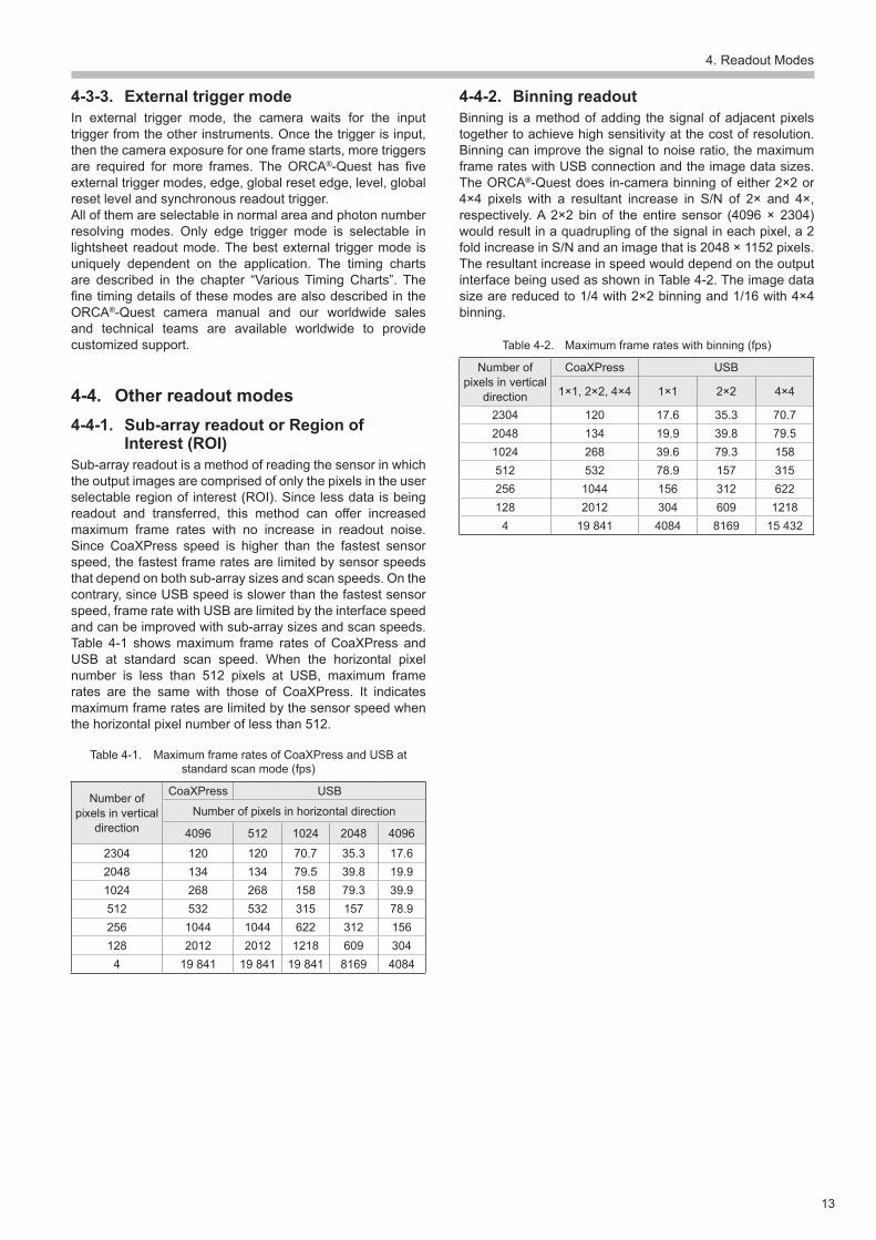
Interest (ROI)Sub-arrayreadoutisamethodofreadingthesensorinwhichtheoutputimagesarecomprisedofonlythepixelsintheuserselectable region of interest (ROI). Since less data is being readout and transferred, this method can offer increasedmaximum frame rates with no increase in readout noise. Since CoaXPress speed is higher than the fastest sensor speed,thefastestframeratesarelimitedbysensorspeedsthatdependonbothsub-arraysizesandscanspeeds.Onthecontrary,sinceUSBspeedisslowerthanthefastestsensorspeed,frameratewithUSBarelimitedbytheinterfacespeedandcanbeimprovedwithsub-arraysizesandscanspeeds.Table 4-1 shows maximum frame rates of CoaXPress and USB at standard scan speed. When the horizontal pixel number is less than 512 pixels at USB, maximum frame rates are the same with those of CoaXPress. It indicates maximumframeratesarelimitedbythesensorspeedwhenthe horizontal pixel number of less than 512.

Table 4-1. Maximum frame rates of CoaXPress and USB at standard scan mode (fps)

Number of pixels in vertical

direction

CoaXPress USB

Number of pixels in horizontal direction

4096 512 1024 2048 40962304 120 120 70.7 35.3 17.62048 134 134 79.5 39.8 19.91024 268 268 158 79.3 39.9512 532 532 315 157 78.9256 1044 1044 622 312 156128 2012 2012 1218 609 304

4 19 841 19 841 19 841 8169 4084

4-4-2. Binning readoutBinning is a method of adding the signal of adjacent pixels togethertoachievehighsensitivityatthecostofresolution.Binning can improve the signal to noise ratio, the maximum frame rates with USB connection and the image data sizes. The ORCA®-Questdoes in-camerabinningofeither2×2or4×4 pixels with a resultant increase in S/N of 2× and 4×,respectively.A 2×2 bin of the entire sensor (4096 × 2304)would result in a quadrupling of the signal in each pixel, a 2 foldincreaseinS/Nandanimagethatis2048×1152pixels.The resultant increase in speed would depend on the output interface being used as shown in Table 4-2. The image data sizearereducedto1/4with2×2binningand1/16with4×4binning.

Table 4-2. Maximum frame rates with binning (fps)

Number of pixels in vertical

direction

CoaXPress USB

1×1,2×2,4×4 1×1 2×2 4×4

2304 120 17.6 35.3 70.72048 134 19.9 39.8 79.51024 268 39.6 79.3 158512 532 78.9 157 315256 1044 156 312 622128 2012 304 609 1218

4 19 841 4084 8169 15 432

5.Synchronization

14

5. Synchronization

5-1. Synchronization with other instruments

As a camera is just one piece of a complicated imaging system,itisoftennecessaryforittobeusedinsynchronizationwith other instruments. In some cases, the other instrument is a camera. The fastest synchronization is establishedwith an electrical signal by connecting the cable betweenthe instruments. In synchronization, only one instrumentbecomes a master, including cameras, and all others become slave instruments.

5-1-1. Use the camera as a slave instrumentExternal trigger mode is the operation mode used when the ORCA®-Quest is a slave instrument. The camera has a trigger input connector and is synchronizedwith the pulsefrom other instruments.

5-1-2. Use the camera as a master instrumentThere are three operation modes in which the ORCA®-Quest isusedasamasterinstrument.Thefirstisfreerunningmode,the second is start trigger mode and the last is external trigger modewiththemasterpulse.Theyallusetheinternaltriggergenerated inside the camera. The camera has three trigger outputconnectorsand three typesof triggeroutputsignalsareselectableforsynchronizationswithotherinstruments.

5-2. Trigger inputTosynchronizethecamerawithotherinstruments,thecamerauses the trigger input signal from the other instruments through the trigger input connector. The signal level needs TTL or 3.3 V LVCMOS and both positive and negative polarity isselectable.Theinput triggercanbedelayedwiththeprogramabledelayedtimeof0μsto10sby1μsstep.Trigger times is a function that allows the number of enabled triggerstobereducedbytheratioofthetimesnumber.Forexample, if the Trigger times is four, three trigger inputs are ignored, and the next trigger input is enabled.

5-3. Trigger outputTosynchronizeotherinstrumentswiththecamera,ORCA®-Quest has three trigger output connectors and various trigger output signals.

5-3-1. Global exposure timing outputThecamerasimultaneouslyoutputstheperiodwhereallrowsare exposed. Since the timing of the exposure in each row is differentfortherollingshutter,itispossiblethataphenomenonmaybeobservedpartiallyineachoftwoconsecutiveframes.Globalexposuretimingallowsforsynchronizingoftheeventto the time when all rows are exposing, therefore moving the event into a single frame. Exposure should be set to longer thanthereadouttotakeadvantageofthissynchronization.

Internal exposure timing settingExtarnal trigger

*Delay and Jitter

Sensor readoutCoaXPress data output

USB data outputGlobal exposure timing output

Any-row exposure timing outputTrigger ready output (CoaXPress)

Trigger ready output (USB)

0(H)1(H)

N-1(H)N(H)

Fig. 5-1. Global exposure timing output

5-3-2. Any row exposure timing outputSincethetimingoftheexposureineachrowisdifferentforthe rolling shutter, the total exposure period from the start to the end of all rows is longer than the exposure time of a single row.Anyrowexposuretimingoutputgivesthestartandendtiming of the total exposure period of all rows and it is useful forsynchronizingwithotherinstruments.

5-3-3. Trigger ready outputWhen operating in external trigger mode, the interval from one exposure to the next can be shortened with the use of the trigger ready output.When the camera is operating inexternal trigger mode, for example for the edge trigger, the next exposure will start only after the sensor readout hasended. For this reason, a trigger for the start of the next exposure cannot be accepted during an exposure or readout. Bymonitoringtheoutputsignalattheendofreadouttheinputtriggermaybesentimmediatelytostartthenextexposure,toreduce the dead time as much as possible.

5.Synchronization

15

5-3-4. Programmable timing outputFor the programmable timing output, pulses with a delaytimeandpulsewidtharesetbyacommand,andreferencedto the user selection of the end of the sensor readout, Vsync (vertical synchronous signal) or Hsync (horizontalsynchronous signal). By using the programmable timingoutput,simplesynchronizationwithexternaldeviceswillbeenabled,allowing it to replaceasimpledelayunitorpulsegenerator.Thesettingrangeofthetimedelayis0μsto10s,andpulsewidthis10μsto10s.

Extarnal trigger

Sensor readout

Read end

Vsync

Trigger

0(H)1(H)

N-1(H)N(H)

Delay Width

Delay Width

Delay Width

Fig. 5-2. Programmable timing output (normal area mode, edge trigger)

5-3-5. Pre-HsyncIn lightsheet readout mode, a timing signal referenced to therowreadoutmaybeoutputbysettingtheHsyncoutputtrigger.Thedelayandwidtharesetbycommand.Inaddition,thestartofthelightsheetreadoutmodemaybedelayedbysettinganumberofPre-Hsyncpulses.

Extarnal trigger

Hsync

PreHsync Pulse Num

0(H)1(H)

N-1(H)N(H)

DelayWidth

Fig. 5-3. Pre-Hsync

5-4. Master pulse5-4-1. Master pulseInsomeconventionalsystems,anadditionalexternalpulsegenerator is required tosynchronize thecameraandotherinstruments. The ORCA®-Quest has a master pulse function which can generate pulses that are independent of the exposure or readout timing of the image sensor. The camera canbesynchronizedwiththemasterpulseinexternaltriggermode, except for lightsheet readout mode. The camera can alsooutputtriggerswhicharesynchronizedwiththemasterpulse.

5-4-2. Two cameras simultaneous exposure without an external pulse generator

The master pulse can realize simultaneous exposure of two cameras without an external pulse generator. When two camerasareconnectedwithatriggercable,thefirstcamerais synchronized with its master pulse, the first cameraoutputsthetriggerpulsesynchronizedwiththemasterpulse,the second camera is synchronizedwith the output triggerfromthefirstcamera, theexposureof twocamerascanbecontrolled to be the same timing.

The first camera

Trigger out

Master pulse

The second camera

Trigger in

Master pulse

The first cameraExposure

The second camera Exposure

Master pulse

Camera timing generator

Camera timing generator

The trigger output from the first camera

Fig. 5-4. Two cameras simultaneous exposure without an external pulse generator

5-4-3. Master pulse functionThe master pulse function can be turned ON and OFF (Default is OFF). The master pulse has three modes, free running mode, start trigger mode and burst mode. The range ofintervaltimeis10μsto10s,andthestepis1μsforthemaster pulse.

6. Data Managements

16

6. Data Managements

6-1. Selectable pixel bit depthUsing 8 bit (256 gray levels) or 12 bit (4096 gray levels)depth is a method to reduce the image data volume to a user significantintensityresolution.12bitdigitaloutput:Thedataisreducedto3/4,ofthe16bitoutput.8bitdigitaloutput:Thedataisreducedto1/2,ofthe16bitoutput.Thus8bitor12bitdigital output can also boost the USB interface frame rates, while reducing image data volume.

Fig. 6-1. LUT OFF

6-2. User selectable Look Up Table (LUT)The reduced 8 or 12 bit-depth acquisition can result in the compressionofpixelintensitydata,therebyreducingintensityresolution. The user-controllable Look Up Table (LUT) can be usedtoregain intensityresolutionbyallowingaselectable,reduced range, of intensities to be mapped into the reduced bit-depth. Selectable LUT is adjustable up to 16 bit-depth resolution.

Fig. 6-2. LUT ON

6-3. Real-time defect pixel correctionAs all CMOS image sensors have defect pixels, the sensor utilized in the ORCA®-Questhasaverysmallratioofdefectpixels to normal pixels. To reduce the effect of the defectpixels, the ORCA®-Quest has a real-time variant pixel correction feature. This correction is performed in real-time with no impact on image readout speed. The correction functioncanbeturnedonoroffusingthesoftware,andthecamera defaults to the ON condition when powered up. User selectable correction levels and associated exposure time examples are listed below.

Table 6-1. Ratio of defect pixel number to be corrected

Correction level for white spots Number of pixels to be corrected

High Thousands of pixelsMedium Tens of pixels

Low Several pixels

6-4. Photo Response Non-Uniformity (PRNU) and Dark Signal Non-Uniformity (DSNU)

Quantitativeaccuracyisarequirementforscientificcameras.In order to achieve excellent quantitative performance, goodlinearity,reducedfixedpatternnoiseandminimalpixeldifferencesareneeded,allowingtheusertoacquireuniformbackground images.Hamamatsu builds in outstanding uniform image qualityusingofourmanyyearsofknowledgeandexperiencewithdigital circuit technology. Our attention to detail deliversoutstanding linearity, especially at low light, and offersimprovedphotonresponsenon-uniformity(PRNU)anddarksignal nonuniformity (DSNU) to minimize pixel differencesandreducefixedpatternnoise.

7. Software Support

17

7. Software Support

7-1. DCAM-API®

ORCA®-QuestissupportedbyDCAM-API®, which is provided as driver software. DCAM-API®supportsmanyHamamatsudigital cameras for scientific measurement, including theORCA®-Quest, and isdesigned toabsorb thedifference intheir properties and to allow control by a common callingmethod. DCAM-API® supports Microsoft Windows® and Linux. Please refer to Hamamatsu software information page at the link below.https://dcam-api.com/structure/ForthelatestdetailedinformationsuchascompatibleOS,I/Fcardandapplicationsoftware,pleasecontactyourlocalsalesrepresentative.

7-2. DCAM-SDK & DCIMG-SDKSDK is a Software Development Kit for the integration of Hamamatsu digital cameras with the customer software. Users,dependingon their requirements,maydevelop theirown application software, for camera control with the DCAM-SDKand for recordingDCIMG fileswith theDCIMG-SDK.DCAM-SDK and DCIMG-SDK can be downloaded from the link below after completion of user registration. The current DCAM-SDK4 and DCIMG-SDK supports C/C++with increased language support expected in near future (includingPython).PleaserefertotheHamamatsusoftwareinformation page at the link below.https://dcam-api.com/dcam-sdk-login/Forthelatestdetailedinformation,pleasecontactyourlocalsales representative.

7-3. Hamamatsu softwareHamamatsuofferssoftwareproductsforusewithallDCAMbased Hamamatsu cameras, dedicated to life science applications:HCImageandHoKaWo;for(bio-)physicsandfor industrial application, our HiPic software is the optimum choice.HSRsoftwarehaslimitedfunctionsandiseasy.Forthe full range of Hamamatsu software, please refer to the followinglink:https://camera.hamamatsu.com/all/en/software/hamamatsu_software/index.html

7-4. Third party software support/optionsAs imaging setups become more complex, software has to notonlytocontrolacamera,butmanyotherdevicessuchasmicroscopes,stagesandfilterwheels…Therefore,softwarecompanies have integrated Hamamatsu DCAM based camerasintotheirsoftwareproducts.CurrentlytheORCA®-Quest is supported in LabVIEW,MATLAB, and μManager.Thirdpartysoftwareislistedonhere.https://camera.hamamatsu.com/all/en/software/third_party_software/index.html

https://camera.hamamatsu.com/all/en/software/hamamatsu_software/index.html

https://camera.hamamatsu.com/all/en/software/third_party_software/index.html

8. Various Timing Charts

18


8-1. Explanation of timing chartsIn Chapter 8, each imaging mode is described with reference to a timing chart. First, the chapter discusses how to read the timing charts. The horizontal axis in Fig. 8-1 represents the passageof time.Thepart colored inyellow represents theexposureconditionoftheCMOSsensor.Thetopofthefigurerepresents the top of the image of the CMOS sensor, and the bottomofthefigurerepresentsthebottomoftheimageoftheCMOS sensor. As the CMOS sensor controls the exposure in row increments, the transverse timing of the CMOS sensor isomittedinthefigure.Thisfigureshowstheexternaltriggeris input. After inputting an external trigger (1), a sensor readout (readout of the data in the previous frame) is started (2), and the first and second rows (0H, 1H) of the screenwill start exposing at the same time. Refer to the section of “Simultaneous dual-row readout with single direction”. At the end of exposure the sensor reads out and for the frame grabber interface the data output also starts (3). With the passage of time, the sequential readout of previous frames onarow-by-rowbasisandexposureofthenextframestarts.In the period where all rows are exposed (red square in the figure), theglobalexposure timingoutput (4) isenabled. Inaddition, a trigger ready output (5)will be output once thereadout of one frame is completed and the next external trigger reception is enabled, and if USB is connected, USB data output will be output (6).


*Delay and Jitter



Any-row exposure timing outputTrigger ready output (CoaXPress)


0(H)1(H)

N-1(H)N(H)

Fig. 8-1. Camera operation mode

8-2. Standard and Ultra quiet scan modeIn the Ultra quiet scan mode, the readout slope can be adjusted from 8.3 ms to 20 ms, and the fastest frame rate is 5.0frames/s.Asthereisnochangeintherelationshipofeachtrigger input and output other than the readout slope, please see the timing diagrams of Fig. 8-2 for the Ultra quiet scan.

The normal area mode has both Standard and Ultra quiet scanmodes.PhotonnumberresolvingmodeonlyhasUltraquiet scan mode. The lightsheet readout mode has onlyStandard scan mode

0(H)1(H)

N-1(H)N(H)

Internal exposure timing setting

Sensor readout

CoaXPress data output

USB data output

Global exposure timing output

Any-row exposure timing output

Fig. 8-2. Ultra quiet scan mode in free running mode

8-3. Normal area and photon number resolving modes

The normal area mode has both Standard and Ultra quiet scanmodes.PhotonnumberresolvingmodehasonlyUltraquiet scan mode. The timing of both the normal area mode with Ultra quiet scan and photon resolving mode with Ultra quietscanare thesame.ThedifferencebetweenStandardand Ultra quiet scans is the slope of readout.

8-3-1. Free running modeORCA®-Questallowstheexposuretimetobesetbysoftwareand is equipped with a free running mode that operates in the camera itself. The free running mode is equipped with normal readout mode (when the exposure time is longer than the readout time of one frame) and electrical shutter mode (when the exposure time is shorter than the readout time of oneframe).Thesemodesautomaticallyswitchaccordingtothe exposure time setting.


19

8-3-1-1. Normal readout modeThe normal readout mode is a mode where the set exposure time is either the same as, or longer than the frame readout time. In this case there is the period called global exposure timing in which all pixels are exposed at the same. In that timing the global exposure timing output signal will be high. In normal readout mode there is no time when the pixels are not exposing (dead time) because exposure of the next image starts as soon as the pixel is read out.

0(H)1(H)

N-1(H)N(H)





Fig. 8-3. Normal readout mode

8-3-1-2. Electrical shutter modeTheelectricalshuttermode isusedwhenthe light intensityis too high and the output signal overflows in the normalreadout mode. By adjusting the exposure time to shorterthan the frame readout, the output signal can be reduced to a suitable signal level. As the exposure time is shorter than the frame readout time, there is no global exposure timing. The frame rate is at the maximum.

0(H)1(H)

N-1(H)N(H)


Sensor readout




Fig. 8-4. Electrical shutter mode

0(H)1(H)

N-1(H)N(H)


Sensor readout

USB data output



Fig. 8-5. Electrical shutter mode (USB)

8-3-2. External trigger modeAs described in the chapters of Readout modes and synchronizations, the ORCA®-Quest has various external triggermodesforsynchronizationwiththeinputtriggerfromthe other instruments.

8-3-2-1. Edge trigger modeThe edge trigger mode is used when performing exposure in synchronizationwithanexternaltriggersignal.Theexposuretime is externally set using the software. In edge triggermode,theexposureofthetoprow(0Hinthefigurebelow)isstartedbytheedge(rising/fallingedge)timingofthetriggersignal input to the camera. Then, after the readout time of the row, exposure of the next row (1 H) starts, after which each rowsuccessivelystartsexposure.Fig.8-6showsthetimingchart of the rising edge example.

0(H)1(H)

N-1(H)N(H)

Extarnal trigger


Trigger ready output (CoaXPress)Trigger ready output (USB)


Sensor readout



*Delay and Jitter

Fig. 8-6. Edge trigger mode

8-3-2-2. Global reset edge trigger modeInglobalresetedgetriggermode,theglobalresetismadebytheedge(rising/fallingedge)ofthetriggersignalinputtothecamera. At the same time, global exposure is started, and the readoutismadebynormalreadoutmode.Thetiming,otherthan reset, is the same as the edge trigger mode.

0(H)1(H)

N-1(H)N(H)

Extarnal trigger

*Delay and Jitter




Sensor readout



Fig. 8-7. Global reset edge mode


20

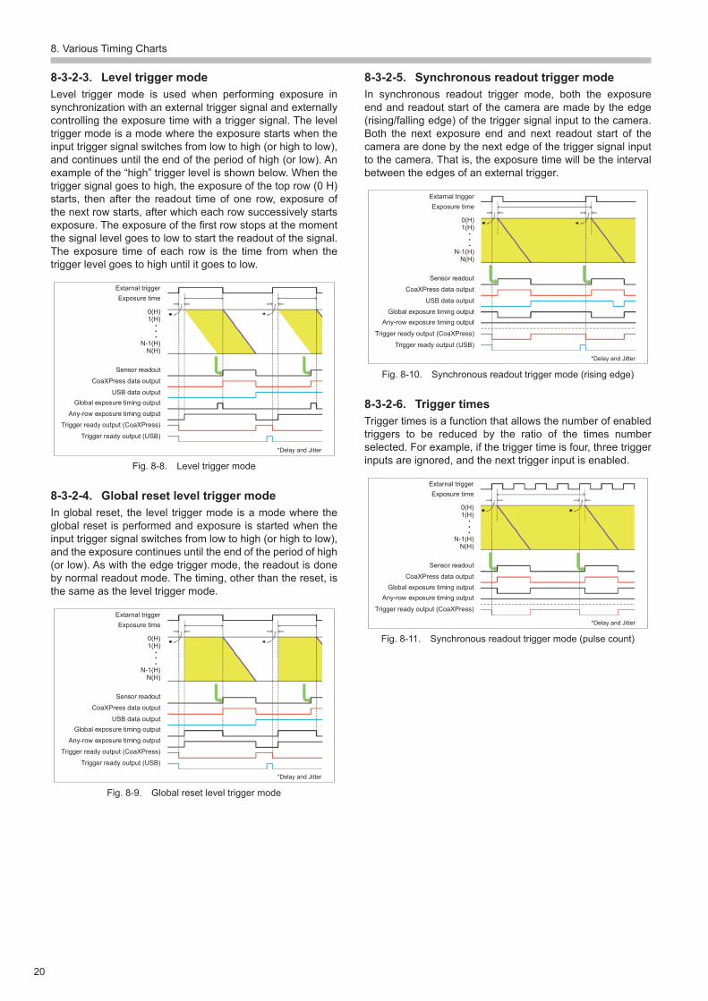
8-3-2-3. Level trigger modeLevel trigger mode is used when performing exposure in synchronizationwithanexternaltriggersignalandexternallycontrolling the exposure time with a trigger signal. The level trigger mode is a mode where the exposure starts when the input trigger signal switches from low to high (or high to low), and continues until the end of the period of high (or low). An example of the “high” trigger level is shown below. When the trigger signal goes to high, the exposure of the top row (0 H) starts, then after the readout time of one row, exposure of thenextrowstarts,afterwhicheachrowsuccessivelystartsexposure.Theexposureofthefirstrowstopsatthemomentthe signal level goes to low to start the readout of the signal. The exposure time of each row is the time from when the trigger level goes to high until it goes to low.

0(H)1(H)

N-1(H)N(H)

Extarnal trigger

*Delay and Jitter



Exposure time

Sensor readout



Fig. 8-8. Level trigger mode

8-3-2-4. Global reset level trigger modeIn global reset, the level trigger mode is a mode where the global reset is performed and exposure is started when the input trigger signal switches from low to high (or high to low), and the exposure continues until the end of the period of high (or low). As with the edge trigger mode, the readout is done bynormalreadoutmode.Thetiming,otherthanthereset,isthe same as the level trigger mode.

0(H)1(H)

N-1(H)N(H)

Extarnal trigger

*Delay and Jitter



Exposure time

Sensor readout



Fig. 8-9. Global reset level trigger mode

8-3-2-5. Synchronous readout trigger modeIn synchronous readout trigger mode, both the exposureendandreadoutstartofthecameraaremadebytheedge(rising/fallingedge)ofthetriggersignalinputtothecamera.Both the next exposure end and next readout start of the cameraaredonebythenextedgeofthetriggersignalinputto the camera. That is, the exposure time will be the interval between the edges of an external trigger.

0(H)1(H)

N-1(H)N(H)

Extarnal trigger

*Delay and Jitter



Exposure time

Sensor readout



Fig. 8-10. Synchronousreadouttriggermode(risingedge)

8-3-2-6. Trigger timesTrigger times is a function that allows the number of enabled triggers to be reduced by the ratio of the times numberselected. For example, if the trigger time is four, three trigger inputs are ignored, and the next trigger input is enabled.

0(H)1(H)

N-1(H)N(H)

Extarnal trigger

*Delay and Jitter


Trigger ready output (CoaXPress)

Exposure time

Sensor readout

Global exposure timing outputAny-row exposure timing output

Fig. 8-11. Synchronousreadouttriggermode(pulsecount)


21

8-3-2-7. Start trigger modeStart trigger mode captures continuous images with one externaltriggerpulse,byswitchingthecameraoperationtofree running mode. It is capable of operating at the fastest framerate.Theexposureofthefirstfameissynchronizedtotheexternalinputtrigger(rising/fallingedge).

0(H)1(H)

N-1(H)N(H)

Extarnal trigger

*Delay and Jitter


Trigger ready output (CoaXPress)


Sensor readout

Global exposure timing outputAny-row exposure timing output

USB data output


Fig. 8-12. Start trigger mode (rising edge)

8-4. Lightsheet readout mode8-4-1. Free running modeAs with the normal area mode, this allows the exposure time to be set using the software and is equipped with a free running mode that operates within the camera. In free running mode, the exposure time, readout slope (line interval) and readout direction can be set by the software. In the top to bottomreadout, exposure is performed from row 0 H of the sensor top to 2303 H in 2 H increments. When the exposure ends, readout continues sequentially from row 0H. The readoutslope is used for synchronizing the readout timing in rowswith the light beam scan speed.

0(H)1(H)

N-1(H)N(H)


CoaXPress data outputUSB data output

Sensor readout

Fig. 8-13. Free running mode (top to bottom readout)

8-4-2. Edge trigger modeInedgetriggermode,exposureismadesequentiallyfrom0Hbytheedge(rising/fallingedge)ofthetriggersignalinputtothe camera. When the exposure ends, readout is performed byeachrow.

0(H)1(H)

N-1(H)N(H)


*Delay and Jitter

CoaXPress data outputUSB data output

Trigger ready output (USB)Trigger ready output (CoaXPress)

Sensor readout

Fig. 8-14. Edge trigger mode (top to bottom readout)

8-4-3. Start trigger modeThe start trigger mode is used when controlling the timing for externallystartingtheimagecaptureaswiththenormalareamode. In the start trigger mode, the exposure of the camera is started at the same time as the camera is switched to the free running by the edge (rising/falling edge) of the triggersignal input to the camera.

0(H)1(H)

N-1(H)N(H)

Extarnal trigger

*Delay and Jitter




Sensor readout

USB data outputTrigger ready output (CoaXPress)

Fig. 8-15. Start trigger mode (top to bottom readout)

9. Understanding SNR

22

9. Understanding SNR

9-1. SNRNo single technical specification can provide all theinformation needed to match a camera to an application. Howeverwhenquantumefficiencyandnoisecharacteristicsof a camera are considered in light of the signal and signal noise, we can understand the theoretical limits of a camera under the full range of light conditions. The signal to noise ratio (SNR) provides tremendous value in predicting which camera performs best for certain applications, assuming the light levels for that application are known.

SNRisdefinedastheratioofthetotalsignaltothetotalnoise.SNRs including EM-CCDs are calculated with Equation 9-1. In the equation, QE is quantum efficiency (%/100), S isinputphotonnumber(photons/pixel),Fnistheexcessnoisefactor (EM-CCD Fn=1.4, others Fn=1), Ib is background (photons/pixel),Nrisreadoutnoise(electronrms),Misthemultiplication gain of EM-CCD (M=1 for CCD or sCMOS). The equation omits the dark current and also applies when the dark current is much smaller than the signal or background such as a short exposure time. For more detailed info please see our ORCA®-Flash4.0 White Paper.

Equation 9-1. Equation of SNR

9-2. rSNRTo make SNR data even more approachable, a useful variation is to look at relative SNR (rSNR), where all data is normalizedtoanimaginary“perfectcamera”thathas100%QE and zero readout noise.Withthistransformation,itiseasytoseethatatalllightlevelswhich are 0.1 photons per pixel or higher with 0 background, the ORCA®-QuesthasbetterSNRthanEM-CCDs.Especiallyat light levels below 3 photons per pixel, the ORCA®-Quest delivers the best SNR of all sCMOS cameras.

0.0

0.1

0.2

0.3

0.4

0.5

0.6

0.7

0.8

0.9

1.0

1.1

0.1 1 10 100

rSN

R

Average number of photons (per pixel)

Relative SNR (Relative to perfect camera)

Perfect camera QE=100 %, RN=0 e-ORCA®-Quest (Ultra quiet) QE=90 %, RN=0.27 e-ORCA®-Fusion BT QE=95 %, RN=0.7 e-ORCA®-Fusion QE=80 %, RN=0.7e-Gen II BSI sCMOS camera QE=95 %, RN=1.8 e-Gen II sCMOS camera QE=82 %, RN=1.4 e-EM-CCD camera QE=92 %, RN=0.1 e-

Fig. 9-1. Relative SNRs of various cameras

9-3. Camera Simulation EngineTo help to easily understand SNR, a “Camera SimulationEngine” is available in our website, please see the following link:https://camera.hamamatsu.com/all/en/camera_simulation_engine/index.htmlThisenginecanproducesimulationimagesbyselectingtheparameters of QE, readout noise, dark noise, excess noise, exposure time, input photon numbers, etc. The images are made by calculating signal and noises that are based onanSNRequation. It providesaeasy to follow, visualSNRcomparisonofmanycameras.

https://camera.hamamatsu.com/all/en/camera_simulation_engine/index.html

https://www.hamamatsu.com/resources/pdf/sys/e_flash4_whitepaper.pdf

10. Application Examples

23


10-1. Quantum technology (Neutral atom, Ion trap)

Neutral atoms and ions can be regarded as so-called qubits because they can take on a superposition state in whicheven a single atom has multiple properties. This propertyisbeingactively investigatedtorealizequantumcomputingand quantum simulation. Observing the fluorescence fromtrapped ions and neutral atoms with a low-noise camera is often used for determining the state of the qubit.Fig. 10-1. shows a simulated image example of Rb atoms. Twenty-fiveRbatomsarepositionedina5×5arraywith5μmdistance each. In this simulation, each atom is the source for 2000photonsat780nmandis imagedbya20×(NA:0.4)objective onto an ORCA®-Questpixelarray,withanadded5photons/pixelbackgroundsignal.

Fig. 10-1. A simulated image example of neutral atoms

10-2. Astronomy (Lucky / Speckle imaging)When observing stars from the ground, it is very hard tocapture clear star images with long exposure because the imagesareblurredbyatmospheric turbulence. In contrast,clear images are sometimes captured with short exposure when those exposures match with atmospheric conditions. Lucky imaging is a method of acquiring a large stack ofimages. It then uses a subset of these images which have the least amount of atmospheric turbulence, shifts the brightest points to the same reference position and then averages the subset together to make a higher resolution image.Fig. 10-2. shows an example image of Orion Nebula captured byluckyimagingwith3colorfilters.

Fig. 10-2. LuckyimagingofOrionNebula

10-3. Lifescience(Delayedfluorescenceof plants)

Plants release a very small portion of the absorbed lightenergy, through photosynthesis, as photons over a longtime.Thisphenomenon isknownasdelayedfluorescence.Detecting those photons makes it possible to observe the effectsofchemicals,pathogens,theenvironment,andotherstress factors on plants.Fig.10-3.showsadelayedfluorescenceexampleofornamentalplants. The image is taken with 10 s exposure after 10 s has passedfromwhentheexcitationlightisturnedoff.

Fig. 10-3. Plantphoton(delayedfluorescence)


24

10-4. Raman spectroscopyRamaneffectisascatteringoflight,thewavelengthofwhichis shifted away from that of the incident light, andRamanspectroscopy is a technique for determining the materialproperties by measuring this wavelength shift. Ramanspectroscopy enables structural analysis at the molecularlevel, which provides information on chemical bonding, crystallinity,etc.Fig.10-4.showsanexampleofaRamaneffect imageandthe resulting spectrum for acetone. Since Raman scattering isveryweak,lownoisecamerasarenecessaryfordetecting.In addition, since the wavelength shift is small, high resolution andlargepixelnumbersarenecessaryforthisapplication.

Average Raman spectrum of the straight line(10 pixels vertically)

0

50

100

150

200

250

300

350

300500700900110013001500

Ramanshift/cm-1

Cou

nt

Raman spectrum image of acetone

04000 3600 3200 2800 2400 2000 1600 1200 800 400 0

200

400

600

800

1000

1200

1400

1600

1800

2000

2200

500

400

300

200

100

0

Fig. 10-4. An example of Raman spectrum

11.Specifications

25

11. Specifications

11-1. Specificationchart

Product number C15550-20UPImaging device qCMOS® image sensorEffectivenumberofpixels 4096(H)×2304(V)Pixel size 4.6μm(H)×4.6μm(V)Effectivearea 18.841mm(H)×10.598mm(V)Quantumefficiency(typ.) 90 % (peak QE)Fullwellcapacity(typ.) 7000 electronsReadoutnoise(typ.) Standard scan 0.43 electrons rms

Ultra quiet scan 0.27 electrons rmsDynamicrange(typ.)*1 25900:1Darksignalnon-uniformity(DSNU)(typ.)*2 0.06 electrons rmsPhotoresponsenon-uniformity(PRNU)(typ.)*2*3 0.1 % rmsLinearityerror EMVA1288standard(typ.) 0.5 %

Cooling Sensor temperature Darkcurrent(typ.)Forced-aircooled(Ambienttemperature:+25°C) −20°C 0.016electrons/pixels/sWatercooled(Watertemperature:+25°C) −20°C 0.016electrons/pixels/sWatercooled(maxcooling)(typ.)*4 −35°C 0.006electrons/pixels/s

At Normal area readout and Photon number resolvingReadout mode Fullresolution,Digitalbinning(2×2,4×4),Sub-arrayFrame rate at full resolution Standard scan *5 120frames/s(CoaXPress),17.6frames/s(USB)

Ultra quiet scan 5frames/s(CoaXPress,USB)Exposure time Standard scan *5 7.2μsto1800s

Ultra quiet scan 199.9 ms to 1800 s *6

Trigger input External trigger input mode Edge/Globalresetedge/Level/Globalresetlevel /Syncreadout/Start

Software trigger Edge/Globalresetedge/StartTriggerdelayfunction 0sto10sin1μssteps

At Lightsheet readout *7

Readout mode Fullresolution,Sub-arrayRow interval time 7.2μsto237.6μsExposure time 7.2μsto271.872msTrigger input External trigger input mode Edge/Start

Software trigger Edge/StartTriggerdelayfunction 0sto10sin1μssteps

11.Specifications

26

Trigger output Global exposure timing output / Any-row exposure timingoutput/Triggerreadyoutput/3programmabletimingoutputs/Highoutput/Lowoutput

Master pulse Pulse mode Freerunning/Starttrigger/BurstPulse interval 5μsto10sin1μsstepBurst count 1 to 65 535

Digital output 16bit/12bit/8bitImage processing function Defect pixel correction

(ON or OFF, hot pixel correction 3 steps)Interface USB 3.1 Gen 1, CoaXPress (Quad CXP-6)Trigger input connector SMATrigger output connector SMALens mount C-mountPowersupply AC100VtoAC240V,50Hz/60HzPower consumption Approx. 155 VAAmbient operating temperature 0 °C to +40 °CAmbientoperatinghumidity 30 % to 80 % (With no condensation)Ambient storage temperature −10°Cto+50°CAmbientstoragehumidity 90 % Max. (With no condensation)

*1:CalculatedfromtheratioofthefullwellcapacityandthereadoutnoiseinUltraquietscan*2:InUltraquietscan*3:At3500electrons,thecenter1500×1500areaoftheimagesensor,1000timesintegration*4:Thewatertemperatureis+20˚Candtheambienttemperatureis+20˚C*5:Normalareareadoutmodeonly*6:Whenglobalresetedgeorglobalresetleveltriggerisselected,theexposuretimeis172.8µsto1800s.Whensyncreadout

trigger is selected, 200.2 ms to 1800 s.*7:SoftwaresuchasHCImageisrequired.Fordetails,pleasecontactyourlocalHamamatsurepresentativeordistributor.

11.Specifications

27

11-2. Dimensional Outlines

141.6 10

4.5

18.3 113.632 50

5737 40

405070

4×ϕ4.5 ϕ8 4.53×M6×84×M3×8

1/4-20UNC×8

11055

55 110

8

55

55

4×M4×5

1-32UN×5 C-MOUNT

Camera (Approx. 3.8 kg)

Fig. 11-1. Dimensional outlines

11-3. SystemConfiguration

ORCA®-Quest

C-mount lens

Microscope

software

Water circulator

M9982-30 Frame grabber board CoaXPress 4BNCA14590-05-40 CoaXPress cable DIN-BNC 5 m Set of 4 (with CoaXPress)

C-mountTV adapter

StandardOption

AC adapter M9982-25Frame grabber board

with USB 3.0 A-B 3 m Cable(with USB)

PC

Fig. 11-2. Configurationexample

11-4. OptionsProduct number Product nameM9982-30 Frame grabber board CoaXPress 4BNCA14590-05-40 CoaXPress cable DIN-BNC 5 m Set of 4M9982-25 Frame grabber board with USB 3.0 A-B 3 m CableA12106-05 External trigger cable SMA-BNC 5 mA12107-05 External trigger cable SMA-SMA 5 m

DCAM-API is registered trademark of Hamamatsu Photonics K.K. (EU, Japan, U.K., U.S.A.)ORCAisregisteredtrademarkofHamamatsuPhotonicsK.K.(China,France,Germany,Japan,U.K.,U.S.A.) qCMOS is registered trademark of Hamamatsu Photonics K.K. (China, EU, Japan, U.K.) Windows is registered trademark of Microsoft Corporation in the U.S.A.

Product and software package names noted in this documentation are trademarks or registered trademarks of their respective manufacturers. Subjecttolocaltechnicalrequirementsandregulations,availabilityofproductsincludedinthispromotionalmaterialmayvary.Pleaseconsultyourlocalsalesrepresentative.InformationfurnishedbyHAMAMATSUisbelievedtobereliable.However,noresponsibilityisassumedforpossibleinaccuraciesoromissions. Specificationsandexternalappearancearesubjecttochangewithoutnotice.© 2021 Hamamatsu Photonics K.K.

Cat. No. SCAS0154E03SEP/2021HPKCreated in Japan

HAMAMATSU PHOTONICS K.K.Systems Division812 Joko-cho, Higashi-ku, Hamamatsu City, 431-3196, Japan, Telephone: (81)53-431-0124, Fax: (81)53-433-8031, E-mail: [email protected].: Hamamatsu Corporation: 360 Foothill Road, Bridgewater, NJ 08807, U.S.A., Telephone: (1)908-231-0960, Fax: (1)908-231-1218 E-mail: [email protected]: Hamamatsu Photonics Deutschland GmbH.: Arzbergerstr. 10, 82211 Herrsching am Ammersee, Germany, Telephone: (49)8152-375-0, Fax: (49)8152-265-8 E-mail: [email protected]: Hamamatsu Photonics France S.A.R.L.: 19, Rue du Saule Trapu, Parc du Moulin de Massy, 91882 Massy Cedex, France, Telephone: (33)1 69 53 71 00, Fax: (33)1 69 53 71 10 E-mail: [email protected] Kingdom: Hamamatsu Photonics UK Limited: 2 Howard Court,10 Tewin Road, Welwyn Garden City, Hertfordshire AL7 1BW, UK, Telephone: (44)1707-294888, Fax: (44)1707-325777 E-mail: [email protected] Europe: Hamamatsu Photonics Norden AB: Torshamnsgatan 35 16440 Kista, Sweden, Telephone: (46)8-509 031 00, Fax: (46)8-509 031 01 E-mail: [email protected]: Hamamatsu Photonics Italia S.r.l.: Strada della Moia, 1 int. 6, 20044 Arese (Milano), Italy, Telephone: (39)02-93 58 17 33, Fax: (39)02-93 58 17 41 E-mail: [email protected]: Hamamatsu Photonics (China) Co., Ltd.: 1201 Tower B, Jiaming Center, 27 Dongsanhuan Beilu, Chaoyang District, 100020 Beijing, P.R. China, Telephone: (86)10-6586-6006, Fax: (86)10-6586-2866 E-mail: [email protected]: Hamamatsu Photonics Taiwan Co., Ltd.: 8F-3, No.158, Section 2, Gongdao 5th Road, East District, Hsinchu, 300, Taiwan R.O.C. Telephone: (886)3-659-0080, Fax: (886)3-659-0081 E-mail: [email protected]

www.hamamatsu.com

Documents

ORCA-Quest qCMOS camera C15550-20UP Technical note