Optimisation of Pre-set Forearm EMG Electrode Combinations

Optimisation of Pre-set Forearm EMG

Electrode Combinations using Principal

Component Analysis

Kyle Gavin Hans McWilliam Fyvie

Johannesburg, October 2018

A dissertation submitted to the Faculty of Engineering and the Built Environment,

University of the Witwatersrand, Johannesburg, in fulfilment of the requirements

for the degree of Master of Science in Engineering.

The financial assistance of the National Research Foundation (NRF) towards this

research is hereby acknowledged. Opinions expressed, and conclusions arrived at,

are those of the author and are not necessarily to be attributed to the NRF.

i

Declaration

I declare that this dissertation is my own unaided work. It is being submitted to the

degree of Master of Science in Engineering to the University of the Witwatersrand,

Johannesburg. It has not been submitted before for any degree or examination to

any other University.

....................................................................................................................................

(Signature of Candidate)

……………. day of ………………………… year ………………….

ii

Abstract

Trans-radial amputees struggle daily when it comes to performing one or more of

their activities of daily living (ADLs). Myoelectric prosthetic hands have recently

been developed to a point where they can assist trans-radial amputees to perform

their ADLs, making use of electromyographic (EMG) signals to drive the prosthetic

hand. In order to function, a myoelectric prosthetic hand requires multiple

electrodes to collect EMG data (denoted a channel) from a prosthetic user’s

remaining forearm muscles, as well as complex classification algorithms to process

the data in real time. The focus of research in this field is directed at developing or

improving the classification algorithms, often ignoring the optimisation of the EMG

electrodes themselves. The electrodes can be optimised either by position or

number, however in research where electrodes are optimised, classification

accuracy is used as a measure of success for the optimisation, which requires

optimisation of the classification algorithm itself.

The focus of the current study was to develop a method that could optimise the

EMG electrode placements and number, without needing a classification algorithm.

A pre-existing 8-EMG channel dataset for seven subjects was used. The

experimental method involved generating combinations of two, three and four

channels from which optimal channel combinations were selected. The

optimisation process made use of principal component analysis (PCA), which

generated a reduced-quality model for each potential combination. The

reduced-quality and original models were compared, and the optimal channel

combinations identified from those comparisons with the least error. The success

of the optimisation was defined as the impact that a reduced number of EMG

channels would have on the percentage of variance retained (PVR) by the optimal

channel combinations.

The optimal channels for each subject were compared, and although each subject

displayed variation, in general the important channels were identified as those that

were located over the Extensor digitorum (ED), Flexor pollicis longus (FPL),

Flexor digitorum superficialis (FDS), Flexor digitorum profundis (FDP), and

iii

Extensor carpi ulnaris (ECU) muscles. The optimal channel combinations for all

subjects together had an average of 64.5% PVR for the 2-channel setup, 73.9% for

the 3-channel setup, and 76.5% for the 4-channel setup. This shows that it is

possible to reduce the number of channels and retain a large amount of variance in

the data without the use of classification algorithms.

iv

Acknowledgements

I would like to start by thanking both of my supervisors, Prof Vered Aharonson and

Mr Abdul-Khaaliq Mohamed. Their valuable advice most certainly shaped the

course of this study, and upon the completion of this task I am very grateful for the

guiding approach that they took to assisting me. Being guided to choose my own

topic and define my own research goals and methods was tough to start with, but I

am much more confident in my own abilities as a researcher because of them.

I would also like to acknowledge the National Research Foundation for the financial

assistance that they provided over the course of this project.

I also want to thank my fellow researcher Gabriel for his company while going

through this project, and I hope his journey is as successful as mine.

Lastly but not least, I want to express my appreciation for all the support I have

received from my wife Carmen, my sister Robyn and my parents Guy and Nicky,

throughout the process of completing this project. They have never doubted my

ability to complete it, and have been waiting very patiently for the outcome. I’m

truly glad to have a family like you.

v

Table of Contents

Declaration i

Abstract ii

Acknowledgements iv

Table of Contents v

List of Figures viii

List of Tables x

Glossary of Terms and Abbreviations xi

– Introduction to Study 1

Background to Problem................................................................... 1

Significance ..................................................................................... 4

Dissertation Structure ...................................................................... 4

– Literature Review and Background 7

Electromyography (EMG) .............................................................. 7

2.1.1 Forearm EMG ……………………………………………………... 8

2.1.2 Optimal Electrode Combinations ……..……..……..………..... 9

Principal Component Analysis (PCA) ......................................... 12

2.2.1 PCA on EMG Signals …………………………………………...14

2.2.2 Fixed Effect Model in PCA …………………………………… 15

2.2.3 Data Variance Content of Selected PCs ……………………. 16

Literature Review Summary ......................................................... 16

Background ................................................................................... 17

2.4.1 Signal Error Analysis ……………………………………………17

2.4.2 Muscles of the Forearm and Grasping ……………………….19

Chapter Summary.......................................................................... 22

vi

– Experimental Setup 23

Dataset ........................................................................................... 23

3.1.1 Subjects ……………………………………………………………. 23

3.1.2 Experimental Setup, Hardware and Software ……………... 23

3.1.3 Electrode Placements on the Forearm ………………………. 24

3.1.4 Experimental Procedure and Results ………………………... 25

Data and Function Validation ....................................................... 26

Chapter Summary.......................................................................... 28

– Methods for Identifying Optimal Channel

Combinations 29

Mapping the Grasps ...................................................................... 30

Generation of Channel Combinations ........................................... 32

Error Calculation ........................................................................... 33

Error Analysis ............................................................................... 34

Chapter Summary.......................................................................... 36

– Methods for Graphical Representation of Results 37

Percentage of Variance Retained (PVR) ....................................... 37

Chapter Summary.......................................................................... 38

– Results 39

Subject 1 ........................................................................................ 40

Subject 2 ........................................................................................ 41

Subject 3 ........................................................................................ 42

Subject 4 ........................................................................................ 43

Subject 5 ........................................................................................ 44

Subject 7 ........................................................................................ 45

Subject 8 ........................................................................................ 46

Most Common Channel Combinations ......................................... 47

Average Percentage Variance Retained ........................................ 48

vii

Chapter Summary.......................................................................... 49

– Discussion 50

Updated Electrode Placements on the Forearm ............................ 50

2-Channel Setup Trends ................................................................ 53



Percentage Variance Retained Trends .......................................... 58

Answering the Research Question ................................................ 60

Future Work .................................................................................. 61

Chapter Summary.......................................................................... 62

– Conclusion 64

References 67

Appendix A – Ethics Clearance Certification 74

viii

List of Figures

Figure 1.1: Flow diagram of research goals. Solid lines indicate a splitting up of

goals into smaller parts, dotted lines indicate the use of smaller goals to

answer their parent goals. ..................................................................... 5

Figure 2.1: Adjusting on axes based on direction of greatest variance (the values

are zero-meaned). ............................................................................... 13

Figure 2.2: FDS muscle (blue) below the anterior surface layer (Adapted from [58]).

............................................................................................................ 21

Figure 2.3: FDP-M muscle (blue), FDP-L muscle (orange) and FPL muscle (green)

of the anterior deep layer. Note the distinction between the medial and

lateral parts of FDP, because the index and middle fingers are flexed by

FDP-L and the ring and little fingers are flexed by FDP-M (Adapted

from [59]). .......................................................................................... 21

Figure 2.4: ECRL (blue), ED (red), ECU (green), ECRB (orange), EPL (purple),

APL (light green) and EPB (light blue) of the posterior surface layer

(Adapted from [60]). .......................................................................... 22

Figure 3.1: Individual and combined finger grasps investigated by Khushaba and

Kodagoda [26] (with permission). ..................................................... 25

Figure 3.2: Typical time-series plot of EMG data for some channels within a short

time period.......................................................................................... 26

Figure 3.3: Typical FFT plot of a channel (Subject 8, Trial 3, M Grasp, Channel 5).

............................................................................................................ 27

Figure 4.1: Method overview - the five block elements are each discussed as a

section in Chapter 4 (except for the Input Data block). ..................... 29

Figure 6.1: Subject 1’s PVR for the All Grasps GA. ............................................ 40


ix






Figure 6.8: Average PVR for each subject for each channel combination (coloured

lines), including the average for all subjects (black line). .................. 49

Figure 7.1: Anterior surface view of the right forearm, showing the electrode

placements (numbered red circles) and FDS (blue) (Adapted from [58]).

............................................................................................................ 51

Figure 7.2: Anterior deep view of the right forearm, showing the same electrode

placements as in Figure 7.1 (numbered red circles). Seen here are the

FPL (green), FDP-L (orange) and FDP-M (blue) (Adapted from [59]).

............................................................................................................ 51

Figure 7.3: Posterior surface view of the right forearm, showing the electrodes

placements (numbered red circles). Seen here are ECRL (blue), ED

(red), ECU (green), ECRB (orange), EPL (purple), APL (light green)

and EPB (light blue) (Adapted from [60]). ........................................ 51

Figure 7.4: Anterior deep view of the right forearm, highlighting the notable

channels in yellow (Adapted from [59]). ........................................... 58

Figure 7.5: Anterior surface view of the right forearm, highlighting the notable


Figure 7.6: Posterior surface view of the right forearm, highlighting the notable


x

List of Tables

Table 2.1: Forearm muscles and their actions. ...................................................... 20

Table 3.1: Naik et al. [61] surface muscle and their corresponding EMG electrodes

for the dataset provided by Khushaba and Kodagoda [26]. ............... 24

Table 4.1: Details on the different GA categories, the GAs and the grasps included.

............................................................................................................ 31

Table 4.2: Number of possible combinations when using only two, three or four

channels. ............................................................................................. 32

Table 6.1: Subject 1’s optimal channel combinations for the GAs....................... 40







Table 6.8: Overall most common channels for each subject for the 2-channel, 3-

channel and 4-channel setups. ............................................................ 47

Table 6.9: PVR by each subject for the All Grasps optimal channel combinations,

for the 2-channel, 3-channel and 4-channel setups. ........................... 48

Table 7.1: Muscle-electrode associations used in the current study, including the

deeper active muscles. In some cases, the active muscles are deeper in

the forearm. ........................................................................................ 52

xi

Glossary of Terms and Abbreviations

Abbreviation/Term Full Name/Description

ADL

APL

Activity of daily living

Abductor pollicis longus

CC Correlation coefficient

DOA Degrees of actuation

DOF

ECRB

ECRL

Degrees of freedom

Extensor carpi radialis brevis

Extensor carpi radialis longus

ECU Extensor carpi ulnaris

ED Extensor digitorum

EMG

EPB

EPL

Electromyography

Extensor pollicis brevis

Extensor pollicis longus

FCR Flexor carpi radialis

FCU Flexor carpi ulnaris

FDP Flexor digitorum profundis

FDP-L Flexor digitorum profundis (lateral aspect)

FDP-M Flexor digitorum profundis (medial aspect)

FDS Flexor digitorum superficialis

FEM Fixed effect model

FPL Flexor pollicis longus

GA Grasp analysis

HC Hand close

I Index finger

iEMG Intramuscular electromyography

I-M Index-middle

I-M-R Index-middle-ring

L Little finger

LDA Linear discriminant analysis

M Middle finger

xii

MCA Mutual component analysis

MI Mutual information

M-R Middle-ring

M-R-L Middle-ring-little

MSC Magnitude squared coherence

MUAP Motor unit action potential

NAP Nerve action potential

NRMSE Normalised root mean squared error

PC Principal component

PCA Principal component analysis

PVR Percentage variance retained

R Ring finger

RA1 Research aim 1

RA1-P1 Research aim 1 – part 1

RA1-P2 Research aim 1 – part 2

RA2 Research aim 2

R-L Ring-little

RMSE Root mean squared error

RQ Research question

sEMG Surface electromyography

T Thumb

T-I Thumb-index

T-L Thumb-little

T-M Thumb-middle

TP Time period

T-R Thumb-ring

1

– Introduction to Study

This chapter discusses the background to the problem identified for study in Section

1.1, followed by Section 1.2 which identifies the significance of solving such a

problem. Lastly, Section 1.3 describes the structure that the remainder of this

dissertation takes.

Background to Problem

Trans-radial amputation refers to the loss of any portion of the forearm through

amputation [1]. This type of amputation can occur at several different levels of the

forearm, meaning that different forearm amputees can have different degrees of

residual limb remaining. These differences in degrees of amputation make it

difficult to find a standardised way to assist trans-radial amputees. The challenge

that trans-radial amputees face is the degree (if any) to which they can perform one

or more of the activities of daily living (ADLs) [2]. ADLs involving the hand

include writing (requiring fine motor control of the fingers), typing (requiring

movement of the fingers), lifting a telephone receiver (requiring coarse motor

control of the fingers) or pouring water from a jug (requiring stability of the hand)

[2]. Each ADL requires the fingers to be manipulated in a specific way to achieve

the desired performance. If an ADL requires the fingers/hand to be held stable for

a period of time (such as holding a jug of water), as opposed to a transitional action

(such as typing), the position the fingers maintain is known as a grasp. For some

ADLs the grasps are very similar, for example lifting the telephone receiver and

pouring water from a jug.

In order to simplify the analysis of ADLs, various sets of common grasps have been

defined for the purpose of achieving the ADLs using a functional hand [3]–[5].

Some ADLs can be achieved using these common grasps [2], [3]. Other ADLs may

require the use of a combination of the grasps together in order to generate a more

complex or specialised grasp [4], [6], [7]. Often the grasps that are performed to

achieve ADLs do not require the participation of all the fingers of the hand, such as

2

the case of pressing a button with the index finger or pinching an object between

the thumb and index finger.

Prosthetic hands can be used to assist trans-radial amputees in performing their

ADLs. They are generally programmed to perform a set of grasps, using some form

of input from a user. Of interest are myoelectric prosthetic hands that make use of

electromyographic (EMG) signals as an information source for actuating the

prosthetic hand into a grasp. EMG is the measure of electrical signals generated by

muscle contractions, and are collected by electrodes that are placed on the surface

of the users’ skin, referred to as surface EMG (sEMG), to measure the underlying

muscle [8], [9]. EMG electrodes can also be implanted in the muscles themselves,

known as intramuscular EMG (iEMG) [10]. While iEMG may provide more

accurate measurements of the electrical activity, the implantation requires invasive

measures and this is often not desirable [10]–[12]. The physical EMG electrode is

responsible for collecting data, and the collected data in digital form is known as an

EMG channel.

Given recent progress in myoelectric prosthetic hand technology, multiple different

prosthetic hands are commercially available [13]–[15]. The prosthetic hands are

often complex, allowing for multiple degrees of freedom (DOF) and degrees of

actuation (DOA) to be implemented [3], [16]. These allow for the programmed

generation of many of the grasps needed for ADLs, including individual finger

grasps, which until recently were beyond the prosthetic hands’ capabilities [17].

This means that the prosthetic hands can be programmed to perform grasps with

almost human-like dexterity, but enabling a user to control them with such accuracy

in real-time presents a major challenge [16], [18].

The challenge with controlling a myoelectric prosthetic hand with a high accuracy

in real-time is often the lack of informative EMG data that can be processed to

generate the required control [19]. This can be due to a number of reasons, one of

which is the limitation of potential EMG electrode placement sites on a trans-radial

amputee’s forearm [20], [21]. Studies often make use of more than five EMG

electrodes to measure data [14], [16]. This provides a large amount of data that is

often helpful with classification [22], [23]. However, it is not practical to make use

3

of so many muscle placement sites for real-time EMG data acquisition. This is

because there are often only two or three independent muscle placement sites

available [24] on a trans-radial amputee.

There are generally two methods of overcoming this control challenge. One method

considers the fact that the muscles normally responsible for some grasps may be

atrophied or missing due to the amputation. Studies have made use of a mapping

system that uses alternate forearm muscles usually reserved for controlling other

grasps [13], [24]. These systems map the EMG channel measurements from these

alternate muscles onto the grasps required to perform the ADLs. The problem with

this type of system is two-fold: 1) The muscles in the mapping normally perform

other grasps, so a user must learn to use these muscles for a different purpose. 2)

The learning process is complex, so a user may have trouble using the prosthetic

hand effectively and may reject it [3], [25].

The second method considers the use of a limited number of EMG channels as

inputs to control the prosthetic hand. With such a method, the position of placement

of EMG electrodes on a potential myoelectric prosthetic user’s forearm becomes

imperative to generate good-quality EMG channel data for classification. The

success of such a system depends on what grasps are being classified, and which

muscles are used to generate these grasps. The use of two EMG channels as an input

is the minimum for any useful control, and a number of studies make use of this

[3], [4], [13]. The successful use of a limited number of channels for EMG data

collection requires that the selection of channels be optimised – in terms of both the

physical placements of the electrodes on the relevant muscles, as well as the number

of channels that are used for data collection.

Using intuitive-to-control myoelectric prosthetic hands can enable trans-radial

amputees to perform grasps and achieve their ADLs. However, for the prosthetic

hands to function properly, good-quality EMG channel data, collected from a

limited number of electrode placement sites, is required. Identifying these optimal

sites currently requires a lengthy and complex process of experimental placement

and testing of the resultant EMG channel data. Additionally, the use of

classification algorithms is generally required to validate the optimisation. A

4

potential solution that identifies these optimal EMG electrode placement sites

without the use of a classification algorithm needs to be pursued.

Significance

Many studies that make use of the collection of EMG channel data to control

myoelectric prosthetic hands do not address the possible benefits of selecting an

optimal combination of EMG channels. This may be largely due to the focus of

these studies on the classification of the EMG data, rather than on the quality of the

data. This is because being able to successfully classify sub-optimal data means that

the classification system is robust. Some of the studies that do discuss optimal

electrode placements [17], [26] use a classification system to measure the success

of the optimisation. This poses the challenge of having to optimise the classification

system in addition to the EMG channel selection to be sure that the results are

accurate.

This study aims to identify a new method for optimising the EMG electrode

placement process. This process is to be done prior to the use of a classification

algorithm, to confirm that the EMG channel optimisation was successful. In

addition to determining the most important EMG channels to use for a given set of

grasps, the underlying relevant muscles can also be identified so that future

classification systems may base their EMG electrode placements on the results of

this study.

Dissertation Structure

This study aims to answer the following research question (RQ): In using an

8-channel EMG dataset, what are the optimal combinations of two, three and four

EMG channels that preserve their data variance content when compared to the

original 8-channel dataset?

To answer this question fully, the study is split into two main research aims (RAs).

Research aim 1 (RA1) is as follows: What are the optimal two, three and four

channel combinations for each subject within the dataset, and how good is it

5

compared to the original 8-channel dataset for each subject? And research aim 2

(RA2): Given the two, three and four channel optimal combinations identified in

RA1, which muscles are mainly responsible for generating this EMG data?

Figure 1.1 indicates how the RQ was broken down into goals. The splitting of RA1

into two parts (RA1-P1 and RA1-P2) is discussed when looking at the overview for

Chapter 4 and Chapter 5. The process of answering the RQ is as follows: RA1-P1

is used to answer RA1-P2, and they together answer RA1. Then RA1 is used to

answer RA2, and they together answer the RQ.

Figure 1.1: Flow diagram of research goals. Solid lines indicate a splitting up of goals into

smaller parts, dotted lines indicate the use of smaller goals to answer their parent goals.

To answer these RAs and subsequently the RQ, the rest of the study is structured

as follows:

Chapter 2 looks at the prominent techniques in this study, namely EMG and

principal component analysis (PCA). It explains the concepts behind these

technologies and reviews the relevant literature to define the RQ. In addition, the

background of the signal error metrics used in this study and their definitions are

reviewed, followed by a description of the relevant anatomical muscular structures

of the forearm.

Chapter 3 describes the 8-channel EMG dataset that was used for this study,

including the subjects that participated in the data collection experiment, and the

6

hardware and software used. The chapter further presents information regarding the

placement of electrodes, specifies the limitations of the experimental procedures

and validates the data.

Chapter 4 and Chapter 5 focus on the methodologies used in answering RA1, by

splitting it into two parts, RA1-P1 and RA1-P2. The methodology in Chapter 4

(based on PCA), focusses on RA1-P1: What are the optimal channel combination

trends that can be identified within and across subjects? Following this, Chapter 5

uses the results of Chapter 4 to focus on RA1-P2: How much impact does the

reduction in the number of electrodes have on the variance content of the data?

Chapter 6 presents the results of both RA1-P1 (in a tabular format) and RA1-P2 (in

a graphical format) for each subject that were generated by the methods in Chapter

4 and Chapter 5. Additional results derived from the individual subject results are

presented for discussion.

Chapter 7 discusses the derived results presented in Chapter 6. Following the

discussion, the various goals of this study are answered, using the structure

identified in Figure 1.1.

Chapter 8 concludes the study and identifies potential future work.

7

– Literature Review and

Background

This chapter covers the various concepts and technologies that are used within the

scope of this study. Section 2.1 and Section 2.2 cover the major topics that are tied

directly to the title of the dissertation, namely: EMG and PCA respectively. Section

2.3 relates the RQ defined in Chapter 1 to the literature review of these major topics.

Section 2.4 covers the background of other important concepts that complement the

major topics, such as the signal error metric calculations used in this study and the

relevant anatomy of the forearm muscles.

Electromyography (EMG)

Criswell discusses in [12] that the most basic level of organisation with regards to

muscles is the motor unit, which includes a bundle of muscle fibres and their

associated motor neuron from the spinal cord. A nerve action potential (NAP) will

run through the neuron towards the muscle fibre. Upon reaching the muscle the

NAP causes a depolarisation within the muscle fibre, which spreads throughout the

muscle fibre, causing a contraction. This is what is known as a muscle unit action

potential (MUAP). Several MUAPs acting together is what would more generally

be known as a muscle contraction, and this depolarisation is what is being measured

when using EMG. To change the strength of a contraction, a muscle may recruit

different numbers of muscle fibres to be involved. The change in the number of

recruited muscle fibres causes the amplitude of the corresponding EMG recording

to change, since the EMG is recording the combined spatial and temporal

depolarisations of the recruited muscle fibres, rather than a stronger depolarisation

from a single muscle fibre.

There are two different forms of EMG, sEMG and iEMG [11], [12]. iEMG

electrodes are implanted into individual muscles to generate more focussed

recordings [11]. This is noticeable with the amplitude of the electrical signal, given

that measurements using iEMG generate recordings in the range of millivolts versus

8

using sEMG, which measures microvolts [12]. Specifically, the current study

makes use of sEMG (referred to as EMG unless specified otherwise). It is safe and

non-invasive and thus much easier to generate recordings, as the electrodes only

need to be placed on the surface of the skin above the muscle that is being measured

[8], [12]. Although the measurements are not as focussed on individual muscles or

as strong amplitude-wise as iEMG, sEMG is still able to generate meaningful

information. This is because muscles generally work in groups to achieve goals, a

concept known as muscle synergy [27]. Muscle synergy in action is seen in Table

2.1, where multiple muscles work together to produce a grasp, and these muscles

are involved in multiple other grasps as well.

Criswell discusses further [12]: Muscle fibres can work in different ways. There are

three clearly identifiable types of muscle contractions: isometric, concentric and

eccentric. Of interest here is the isometric contraction type, where a constant muscle

length is maintained during contraction. Such a contraction is generally used for

stability and postural control, or during manual muscle testing. EMG recordings are

generally of highest amplitude when the muscle(s) measured are contracting in an

isometric fashion.

2.1.1 Forearm EMG

Given that the muscles of the forearm are responsible for the movements of the

hand at the wrist as well as most of the individual and combined finger movements

and grasps, EMG measurement on the forearm is well documented [12]. Many

studies look at using these EMG measurements as inputs for prosthetic hand

controllers [3], [13], [16], [20], [26], [28], [29]. Understanding the control

mechanisms employed to control the hand is vital to knowing which muscles

become important when certain grasps or movements are performed [30], [31].

There are two general methods of electrode placement when measuring EMG on

the forearm. The first is the general placement method, where the electrodes are

placed on areas of the forearm (determined by anatomical knowledge) or around

the circumference of the forearm [9], [16], [17], [26], [32], [33]. This method relies

on the fact that the placement of the electrodes allows for differential EMG

9

measurements to be taken. This assists in the classification process, since any

classification algorithm relies on the differences within features to be successful

[34]–[36]. The second method is to place the electrodes above specific muscles to

measure them when they contract for a grasp [12]–[14], [37]–[39]. This method

relies on the understanding of what muscles will contract to perform a grasp. This

allows for a stronger EMG signal to be measured and processed for classification.

2.1.2 Optimal Electrode Combinations

The optimisation of EMG electrode placements is a focal point in the realm of EMG

measurements used for prosthetic hands, and they can be optimised in multiple

ways. These optimisations can be the choice of a correct placement of a single

electrode to collect the best quality EMG data, the optimal spatial placement of

several electrodes together, or the reduction of the total number of electrodes.

Reducing the number of electrodes used in measurement is of particular

importance, since a reduction in the number of required inputs for a classification

system reduces its complexity [40]. The importance of the electrode placements

and/or electrode reduction is largely contextual to the application and type of data

collected. Even so, it is useful to be able to compare different datasets and identify

which EMG electrode placement sites remain important throughout different

studies.

Celadon et al. [33] made use of a linear discriminant analysis (LDA) classification

system as a method for selecting an optimal reduced number of EMG electrodes.

EMG data was collected from nine subjects using a sleeve of 192 electrodes,

arranged in eight rings of 24 electrodes around the circumference of the forearm.

The subjects performed tasks involving isometric contractions of the individual

fingers of the dominant hand (not including the thumb), with a visual feedback of

the force produced in their contractions. The tasks included both flexion and

extension contractions while attempting to maintain force to prescribed levels.

There were different inputs tested with the LDA classifier which included a single

ring of the sleeve, two rings of the sleeve, determining the barycentre of EMG

activity (referring to the centre of EMG activity on the sleeve) for each finger during

the tasks, and lastly using all the electrodes available. The results of this study

10

determined that using all the electrodes gave a classification accuracy of more than

91% on average. The performance of the barycentre and two-row methods was

similar, producing a classification accuracy of approximately 82% on average.

Lastly the single-row method gave the worst performance, with a classification

accuracy of 75% on average. It is important to note that while the single row of

electrodes had the worst performance, the use of eight EMG electrodes managed to

give a performance that only had a 16% worse classification accuracy than using

all the EMG electrodes. An explanation for this could be attributed to the lack of

optimisation in the classification system for each subject, not necessarily the

number of electrodes themselves. Even so, the Celadon et al. [33] study showed

that a significant reduction in the number of electrodes was still able to extract most

of the information that was present in the full electrode set.

Andrews [41] focussed on finger movement classification. This included

optimising classifiers for each of twelve subjects, where data for this optimisation

was collected from several typing tasks. It is noted that the generally-optimised

classifiers performed worse than the classifier optimisation for each subject

individually. This work extended into Andrews et al. [17] which focussed on

selecting optimal EMG electrodes from a set of eight around the circumference of

the forearm, using the optimised classifier for each subject. All possible

combinations of eight electrodes were analysed for the classification accuracy. The

results of this study determined that the electrodes placed on Flexor digitorum

profundis (FDP) and Extensor digitorum communis (also known as Extensor

digitorum (ED)) muscles were selected for most often overall. Some of the subjects

didn’t generate a classification accuracy above 50% until they used between five

and seven electrodes. Even so, the Andrews et al. [17] study indicates that using

seven electrodes gives a classification accuracy of 92.7%, which was not

significantly different from the results achieved when using only three electrodes.

Khushaba and Kodagoda [26] proposed optimising the classification of fifteen

finger grasps. Data was collected from eight subjects, using EMG electrodes placed

around the circumference of the forearm. A combined feature selection and

projection algorithm was proposed, called mutual component analysis (MCA).

11

MCA has two stages – firstly a mutual information (MI) algorithm is applied to

determine the information redundancy between two features. If the MI between two

features is high, then one of the features can be discarded without significant loss

to data content. Once MI has been used to rank the features, a second stage using

PCA is applied to remove noisy and redundant features, preserving the features that

exhibit the most variance. The features preserved were run through several different

classifiers to check classification accuracies. MCA reduced the original 168

features to between 42 and 44 features for the eight subjects. The classification

accuracy for this study using the proposed method was above 95% on average

across all subjects, using four or more EMG electrodes. This proves the success of

the system with a greatly reduced number of EMG electrodes. The observation of

the retained features identified that a particular subset of the eight electrodes used

for data collection are important, namely those corresponding to ED, Extensor carpi

ulnaris (ECU), and Flexor carpi ulnaris (FCU). The Khushaba and Kodagoda [26]

study was limited to eight subjects, and so would need to be expanded in future

work to validate the results.

Hargrove et al. [19] investigated the use of iEMG vs sEMG in a classification

system. Six subjects were used, performing ten different movements of the hand

and wrist. Each subject had sixteen sEMG electrodes spaced equally around the

circumference of the forearm (the experimental setup used unipolar electrodes, so

there were fifteen EMG channels), as well as six iEMG electrodes implanted in

muscles. This facilitated the simultaneous collection of EMG data from both

sources. Using multiple classification methods, the study determined that there was

no difference between using six iEMG electrodes and using sixteen sEMG

electrodes. The second part of this study involved identifying optimal sEMG

electrode placements. The study used two different approaches, the first being a

symmetrical selection of subsets of the original fifteen channels, and the second

being a brute-force selection of all possible subsets. Using the symmetrical method

identified that there was no benefit to having more than four electrodes; using the

brute-force method determined that there was no benefit to having more than three

electrodes. The optimal electrode subsets were investigated and the most important

muscles for EMG collection were identified as the Supinator, FCU and Flexor

12

digitorum sublimis, also known as Flexor digitorum superficialis (FDS). Using only

three channels, the study could achieve an average classification accuracy of 97%.

It is noted that the iEMG signals measured were measured from surface muscles,

except for ECU.

Principal Component Analysis (PCA)

PCA is the process of analysing a data table in order to extract important

information that is often not clearly seen in the data [42]. This data table is a matrix

X with rows I and columns J, where each row corresponds to an observation, and

each column corresponds to a variable [42]. PCA decorrelates this multivariate data

and projects it onto a new orthogonal coordinate system, by using the variance

exhibited by the variables [43]. The new coordinate system is defined according to

diminishing variance, where the first dimension is the direction in which the

original data exhibited the highest variance, and the orthogonal dimensions will

exhibit diminishing variance of the original data [43]. Viewing the data on this new

coordinate system allows for correlations/redundancies in the data to be more

clearly seen, and compression of the data can be performed without losing too much

of the information within the original data [44]. Compression in this context refers

to the removal of dimensions/axes that explain to a lesser degree the variance in the

data as a whole, leaving only a subset of the dimensions from the original system

[42]. To achieve this, it is common practice to keep only a few of the highest

variance dimensions that together explain a desired amount of variance. The rest of

the dimensions are removed from the data [45].

Smith [44] briefly describes the process of performing PCA. Once some form of

multivariate data has been collected, the mean of each column J is subtracted from

the values for that column. This ensures that the dataset’s mean is zero, which is

important when considering that some variables may exhibit a form of bias. The

covariance shown in Equation 1 (adapted from [44]) is calculated between each

column in J:

𝐶𝑂𝑉(𝑥, 𝑦) =∑ (𝑥𝑖 − �̅�)(𝑦𝑖 − �̅�)𝑛

𝑖=1

(𝑛 − 1)(1)

13

Where x and y are the columns being compared, and n is the number of observations

(number of rows I). The calculation of the covariance between all columns J

generates a covariance matrix.

Each column of the covariance matrix represents an eigenvector, and each

eigenvector has an associated eigenvalue. The eigenvectors are re-ordered from

high to low according to their eigenvalues. The eigenvalues represent the amount

of variance that is described by the new coordinate system, the axes of which

overlap on each of the eigenvectors. These re-organised eigenvectors and

eigenvalues are denoted the principal components (PCs). The data can then be

mapped onto this new coordinate system, which will more clearly show the

variance in the data, shown in a 2-dimensional example in Figure 2.1. In addition,

dimensions that display minimal amounts of variance can be removed, so that the

data can be viewed with only the most important variances present.

Figure 2.1: Adjusting on axes based on direction of greatest variance (the values are

zero-meaned).

Smith [44] further describes how the removal of minimal-variance dimensions can

be viewed in light of their impact on the data in the original coordinate system. This

is particularly important when the PCA transform is used for data compression. The

covariance matrix that was previously generated is used to reverse the mapping of

the data, and the original mean is added back in to give the data points their original

bias. Now that the reduced-dimension data has been remapped to the original

coordinates, it can be visualised and compared to the original-dimension data.

14

It is important to note the terminology that EMG studies generally use for PCA.

The variables of the columns J correspond to the specific EMG channels. Each

observation in the row I corresponds to a timestamp within the collected EMG data.

2.2.1 PCA on EMG Signals

PCA is often used as an analysis tool for EMG signals, more specifically in the

current study, the forearm muscles. The large number of muscles in the forearm

don’t work independently, rather they assist each other to achieve tasks [46]. This

is known as muscular or neuromotor synergy, which is a common basis for the use

of PCA on EMG signals, since PCA is able to identify these synergies [6]. Muscular

synergy may be broadly defined in two categories [47]. Goal-directed synergy

considers a unit (of synergy) to consist of components (in this case, muscles) that

work together to form a net output [47]. The muscles of the synergy unit may work

in different spatial and temporal combinations, but any synergies developed are

considered to be equivalent so long as the net outputs are the same [47]. The other

synergy is morphological synergy, which focuses on the importance of the spatial

and temporal activity of the individual muscles [47]. In contrast to goal-directed

synergy, two synergies are not considered to be equivalent unless their spatial and

temporal profiles match exactly [47]. Musculoskeletal systems in general have

many DOFs. The implementation of a controller that can map a nearly infinite

number of behavioural movement goals onto an equally large number of muscle

contractions can be extremely difficult [27]. Muscle synergy and PCA are

techniques used to reduce the number of dimensions that such a system needs to

process. In particular, goal-directed synergy is used since it can describe the same

set of muscles differently depending on their activation sequences [27].

Artemiadis and Kyriakopoulos [48] focussed on a three-dimensional mapping of

the shoulder and elbow joints using a magnetic position-tracking system. This

mapping is correlated to the activation of nine muscles, which are all measured

using EMG. The use of PCA in this study is two-fold: 1) To reduce the

dimensionality of the EMG data, since the first and second PCs contained 95% of

the variance data, and 2) to reduce the dimensionality of the joint angle data, where

the first and second PCs contained 93% of the variance data.

15

Zhang et al. [49] based their study on the dimensionality reduction achieved by

Artemiadis and Kyriakopoulos. The study reported that it was only possible to

reduce from eight dimensions of EMG to five, while maintaining 95% of the

variance data. This dimensionality reduction is applied before the generation of

features for a classification system. PCA is noted for having an impact on the

classification accuracy of the motions investigated, however the movements

investigated were of the shoulder and elbow joints. The discussion of the Zhang et

al. study evaluates this use of PCA on EMG signals for dimensionality reduction.

2.2.2 Fixed Effect Model in PCA

A fixed effect model (FEM) is a popular statistical model, that assumes that there

is only one true effect that interacts with all the observations or timestamps in an

analysis. All the observed differences in this effect are due to a sampling error (also

known as noise as discussed in Section 2.4.1) [50]. In the context of an FEM, PCA

is descriptive, where the amount of variance within the timestamps are explained

by the PCs, and the amount of variance described by a PC indicates its importance

[42]. Using PCA as an FEM means that the quality of the PCA model can be

assessed by comparing a reduced-dimension model (as described in Section 2.2.1)

to the original data [42]. Studies often derive new metrics that can be used to assess

the models, and determine the optimal number of dimensions that the system can

be reduced to [42], [45], [51].

All previously discussed studies that made use of PCA as an FEM aimed to identify

how many PCs are required to retain a certain amount of variance. Those PCs that

were not required to meet this goal are removed from the model. This is known as

dimensionality reduction. They have not placed a restriction on the number of PCs

that need to be retained. The current study does not use PCA to reduce

dimensionality (with a variable number of PCs), but instead places a restriction on

the number of PCs intentionally to reduce the quality of the reduced-dimension

model. This allows for a greater deviation in values when compared to the original

data. When the data is reconstructed to the original coordinate system, the deviation

in data quality allows the original-dimension model and the reduced-dimension

model to be compared using some form of error metric. A minimal error in this case

16

indicates that the reduced-dimension model more accurately resembles the original-

dimension model. Multiple error metrics are used in the current study for this

purpose, which are described in Section 2.4.1.

2.2.3 Data Variance Content of Selected PCs

As discussed, PCA operates on the variance that the analysed data exhibits.

Covariance is a measure of the variance that is exhibited by two variables [44]. To

extend the concept of covariance further, a covariance matrix is used where all

variables are represented on the row and column, and the cells are filled with the

computed covariances of all variable pairs [44].

The trace of a square matrix refers to the sum of all the diagonal elements in the

matrix [52]. In a covariance matrix these diagonal elements are the variances of

each individual variable, thus the trace is a measure of the total amount of variance

exhibited by all the variables of the covariance matrix [52]. To determine how much

variance is attributed to a subset of variables, the variances of the variables in

question can be divided by the trace of the covariance matrix and presented as a

percentage [53]. This process is useful to determine the relative contribution of each

variable to the information content of a system in terms of variance [53].

Literature Review Summary

The studies involving EMG generally attempted to use the acquired EMG data as

inputs to classification algorithms. The classification algorithms were used to drive

a myoelectric prosthetic hand. In each of these studies, there is an optimisation of

the EMG electrode placement and/or the number of EMG electrodes, making use

of the classification accuracy as a metric for success. The current study attempts to

achieve an optimisation without resorting to the use of a classification algorithm to

verify the success of the optimisation.

Each of the studies discussed in this chapter introduced some form of optimisation

for their EMG data, and their results suggested that most EMG datasets can be

optimised. In particular, the data used in the current study is provided by Khushaba

and Kodagoda [26]. Where they used a classification system to optimise the number

17

of EMG electrodes, the current study did not use a classification system.

Additionally, the muscles that contributed most to the optimised EMG data were

identified by Khushaba and Kodagoda [26]. This allowed for a comparison between

an established classification-based method and a potential non-classification based

method.

PCA is frequently used in EMG processing applications, but usually in the form of

determining a limit for dimensionality reduction for a classification system. In the

current study, PCA was used as an FEM, and the original-dimension and

reduced-dimension models were compared on a variable-by-variable basis using

the three signal error metrics described in Section2.4.1.

Background

The following subsections relate to other concepts and techniques that were used in

the current study, namely signal error analysis and muscles of the forearm.

2.4.1 Signal Error Analysis

Three signal error metrics were prominently used to compare original EMG signals

to 2-PC reconstructed signals, namely: normalised root mean squared error

(NRMSE), correlation coefficient (CC) and magnitude squared coherence (MSC).

The reconstructed EMG signal is considered to have only one type of error – noise

[54]. This is due to the fact that the two signals being compared are not compared

from a cross-session perspective, which reduces the presence of bias and scaling

errors [54]. NRMSE and CC metrics are chosen for their ability to measure noise

effectively, and are measured in the time domain [54]. MSC is a measure of the

energy distribution in the frequency domain [55].

The use of multiple error metrics in combination allows for a “majority vote” to be

applied when choosing optimal channel combinations. This voting system also

helps resolve cases where the three error metrics do not always converge to the

same optimal channel solution. Each error metric is given the same weighting for

this study. Considering alternative weightings for the error metrics is beyond the

scope of this study, and is discussed in Section 7.7.

18

Normalised Root Mean Squared Error

This metric is a variation of the more general root mean squared error (RMSE).

Normalising the RMSE avoids potential problems that can arise if the datasets that

are being compared have differing scales [54], [56]. The equation for the NRMSE

can vary depending on what measure the RMSE is divided by for the normalisation

[54], [56]. The NRMSE used in the current study is shown in Equation 2 (adapted

from [57]):

𝑁𝑅𝑀𝑆𝐸 = √∑ [𝑜(𝑛) − 𝑟(𝑛)]2𝑁

𝑛=1

∑ [𝑜(𝑛)]2𝑁𝑛=1

(𝟐)

Where o(n) is the original EMG signal, r(n) is the reconstructed EMG signal, and

N is the number of time points over which the analysis was performed. The error

value is generally found to be between 0 and 1, but in cases where r(n) and o(n) are

completely opposite the error value may be greater than 1.

Correlation Coefficient

This metric measures how closely two signals change with each other. In this case,

the output from Equation 3 (adapted from [57]) needs to be as big as possible,

indicating a close relationship.

𝐶𝐶 = 𝑐𝑜𝑣(𝑜, 𝑟)

𝜎𝑜𝜎𝑟

(3)

Where cov(o,r) is the covariance of the original EMG signal and the reconstructed

EMG signal. σo and σr are the standard deviations of the original EMG and

reconstructed EMG signals respectively. The output value is bound between 0 and

1.

Magnitude Squared Coherence

This is a measure of the correlation between two signals based on their energy

distribution in the frequency domain [55]. In this case, the output from Equation 4

(adapted from [57]) needs to be as big as possible, indicating a close relationship in

terms of the frequency content.

19

𝑀𝑆𝐶 = |𝑃𝑜𝑟(𝑓)|2

𝑃𝑜(𝑓)𝑃𝑟(𝑓)(4)

Where Por(f) is the cross power spectral density of the original EMG signal and the

reconstructed EMG signal. Po(f) and Pr(f) are the power spectral density of the

original EMG signal and the reconstructed EMG signal respectively. The output

value is bound between 0 and 1.

2.4.2 Muscles of the Forearm and Grasping

The discussion in this section is based on Moore et al. [46]. To understand the hand

movements and grasps used to perform ADLs, an understanding of the musculature

involved is needed. Muscles are only able to pull in a single direction during

contraction, so the degree of involvement that a single muscle has in performing a

grasp is strongly correlated to its location. The largest group of muscles involved

in performing movements related to the fingers are in the forearm.

Commonly, the forearm is divided into two compartments, namely the flexor

compartment and the extensor compartment. These compartments are split by the

ulna and radius bones, along with the interosseous membrane between the two

bones. The flexor compartment contains the muscles involved in flexing the fingers

or closing the hand. The extensor compartment houses the muscles involved in

extending the fingers or opening the hand. Table 2.1 lists the main muscles of the

forearm involved in these movements, excluding some of the more specialised,

smaller muscles that are not considered relevant. Note that this study is only

concerned with the flexion and extension of the finger; however, the listed muscles

also perform other actions such as flexion and extension of the wrist. These

movements are not relevant to this study and are therefore excluded.

20

Table 2.1: Forearm muscles and their actions.

Compartment Muscle Name Shorthand

Name

Action(s)

Flexor Flexor digitorum

superficialis

FDS index, middle, ring and

little finger flexion

Flexor digitorum

profundis (lateral)

FDP-L index and middle finger

flexion

Flexor digitorum

profundis (medial)

FDP-M ring and little finger

flexion

Flexor pollicis

longus

FPL thumb flexion

Extensor Extensor digitorum ED index, middle, ring and

little finger extension (all

together is hand opening)

Extensor carpi

radialis longus

ECRL hand closing

Extensor carpi

radialis brevis

ECRB hand closing

Extensor carpi

ulnaris

ECU hand closing

Abductor pollicis

longus

APL thumb extension

Extensor pollicis

brevis

EPB thumb extension

Extensor pollicis

longus

EPL thumb extension

The flexor compartment is split into three layers; the surface layer, the intermediate

layer, and the deep layer. The surface layer contains no muscles involved in the

hand and finger movements. Figure 2.2 shows the right forearm anteriorly, from

the surface perspective.

21

Figure 2.3 shows the third, deep layer of the right forearm with surface muscles

removed.

The extensor compartment also has layers, but the muscles involved in the finger

and hand movements are on the surface, and so can be seen in Figure 2.4, which

shows the right forearm posteriorly. Note that what is displayed as ED in fact

includes a smaller muscle, Extensor digiti minimi, but for the purposes of this study

this muscle performs it actions alongside ED.

Figure 2.2: FDS muscle (blue) below the anterior surface layer (Adapted from [58]).

Figure 2.3: FDP-M muscle (blue), FDP-L muscle (orange) and FPL muscle (green) of the

anterior deep layer. Note the distinction between the medial and lateral parts of FDP, because

the index and middle fingers are flexed by FDP-L and the ring and little fingers are flexed by

FDP-M (Adapted from [59]).

22

Figure 2.4: ECRL (blue), ED (red), ECU (green), ECRB (orange), EPL (purple), APL (light

green) and EPB (light blue) of the posterior surface layer (Adapted from [60]).

Chapter Summary

EMG is conceptually important to the current study, as it was the method with

which the experimental data was collected, as detailed in Chapter 3. The studies

involving EMG data were focussed on the optimisation of EMG electrodes, through

selecting a reduced number of electrodes and/or identifying important EMG

electrode placement locations. All these studies made use of some form of

classification algorithm to produce a result as to how effective the optimisation was.

The current study attempts to avoid the use of a classification algorithm. It relies

rather on PCA as an FEM to identify important PCs and their variances to identify

optimal electrode locations and channel combinations.

Lastly, the anatomical structure of the relevant forearm muscles is discussed in

general. This is vital to understanding which muscles are involved in which

different types of grasps, when using individual or combinations of fingers. The

correspondence of these muscles to the EMG electrodes used in the dataset is

discussed in Chapter 7, where the optimal channel combinations are discussed. By

extension of having the optimal channel combination results, the active muscles

were identified.

23

– Experimental Setup

This chapter describes and discusses the dataset that was used in the current study.

No EMG data collection was performed. Rather a suitable EMG dataset was

identified and used. Section 3.1 discusses the source that supplied the data. It

includes the details about the subjects, the hardware and software used, the relevant

muscles and EMG electrode placements and lastly the experimental procedure that

was used to collect the EMG data. Section 3.2 discusses the limitations of the

dataset, as well as validations performed.

Dataset

The data used in this study was made available by Khushaba and Kodagoda [26].

Permission for use of this data was provided in the EMG Datasets repository [32],

provided that the corresponding paper is cited. Ethics clearance for the use of the

EMG data was provided by the University of the Witwatersrand, provided in

Appendix A with ethics clearance certificate number M161180. All details

discussed in Sections 3.1.1, 3.1.2 and 3.1.4 are provided by Khushaba and

Kodagoda [26] and the EMG Datasets repository [32].

3.1.1 Subjects

A total of eight subjects (six males and two females) participated in the data

collection process of Khushaba and Kodagoda [26]. The subjects’ ages ranged from

twenty to 35, had no limb abnormalities or amputations, and had no neurological or

muscular disorders. All the participants of the study provided informed consent

prior to their participation in the study.

3.1.2 Experimental Setup, Hardware and Software

Subjects were seated on an armchair, with the arm supported and fixed at one

position for the duration of the data collection process. EMG data was recorded

using eight EMG bipolar electrodes (DE 2.x series EMG sensors) that were

mounted around the circumference of each subject’s forearm, using a two-slot

24

adhesive skin interface to stick the sensors firmly to each subject’s skin. A

conductive adhesive dermatode reference electrode was placed on the wrist of each

subject, on the same arm that the EMG data was recorded from. The collected data

was amplified to a total gain of 1000 (Delsys Bagnoli-8 amplifier). A twelve-bit

ADC (National Instruments, BNC-2090) sampled the signal at 4000 Hz, and the

data was acquired using the Delsys EMGWorks Acquisition software. The data was

processed by the Bagnoli desktop EMG system (Delsys Inc), with a bandpass filter

between 20 Hz and 450 Hz and notch filter at 50 Hz to remove line noise.

3.1.3 Electrode Placements on the Forearm

Note that the electrodes used to collect the data were surface EMG electrodes. The

muscles involved in the hand and finger grasps are not always located near the

forearm surface, and are often located below other muscles. To associate an EMG

electrode with a muscle found deep in the forearm, the muscle located on the surface

of the forearm between them is considered. It is reasonable to assume that the signal

associated with a finger or hand movement can generally be picked up by the EMG

electrode(s) closest to it. Thus, when an electrode measures an EMG signal, the use

of anatomical knowledge on muscle positions and inter-relations can generally

identify the deeper muscle responsible.

The dataset originates from Khushaba and Kodagoda [26], [32], and provides no

reference to the surface muscles the EMG electrodes were placed on. However, a

study by Naik et al. [61] – which also makes use of this EMG dataset – have

proposed the following surface muscle to EMG electrode associations in Table 3.1.

Table 3.1: Naik et al. [61] surface muscles and their corresponding EMG electrodes for the

dataset provided by Khushaba and Kodagoda [26].

Electrode(s) Surface Muscle

1 ED

2 and 3 Brachioradialis

4 Flexor carpi radialis (FCR)

5, 6 and 7 FCU

8 ECU

25

Additionally, Naik et al. [61] proposed that electrodes 1, 2, 7 and 8 be considered

as being located on the posterior aspect of the forearm, where electrodes 3, 4, 5 and

6 are placed on the anterior aspect. In most respects the associations in Table 3.1 as

well as the anterior/posterior identification are carried into the current study,

however some changes to these associations have been proposed and implemented.

These differences are covered in Chapter 7.

3.1.4 Experimental Procedure and Results

A total of fifteen different finger movements were investigated, as shown in Figure

3.1. The movements include flexion of the individual fingers: thumb (T), index (I),

middle (M), ring (R) and little (L). Additional movements are combinations of

fingers: thumb-index (T-I), thumb-middle (T-M), thumb-ring (T-R), thumb-little

(T-L), index-middle (I-M), middle-ring (M-R), ring-little (R-L), index-middle-ring

(I-M-R), middle-ring-little (M-R-L) and a full hand close (HC).

Figure 3.1: Individual and combined finger grasps investigated by Khushaba and Kodagoda

[26] (with permission).

During the data collection process, each subject performed a total of six trials per

grasp (although only three were made available for public use). A single trial

consisted of holding a grasp for a period of twenty seconds (only the first five

seconds were used in Khushaba and Kodagoda [26]). The EMG signals were made

available in the form of csv files, where each file was a single trial for a single grasp

26

for a single subject. The files consisted of the raw data points that were taken over

the twenty second period.

Data and Function Validation

Matlab 2015b was used to import the data from the csv files and to perform all the

processing that will be discussed in this section, as well as in Chapter 4 and Chapter

5. Some processing was performed on the data before it was made available for

public use as described in Section 3.1.2. The quality of the resulting data needed to

be assessed and therefore the following validation process was initially performed:

Visual Inspection of Channel Data

The data was visualised to ensure that each csv data file contains valid data for each

grasp for each subject. Figure 3.2 shows a typical time-series plot that was used for

this visual validation. During the visualisation, it was noted that the datasets for

Subject 6 and Subject 7 were the same for some of the grasps, and in other cases

Subject 6’s data did not look similar in structure to any of the other subjects. For

this reason, it was decided to omit Subject 6’s data from the study.

Figure 3.2: Typical time-series plot of EMG data for some channels within a short time

period.

27

Data Length

Given that twenty seconds of data was collected per grasp at a sampling frequency

of 4000 Hz, each grasp should have 80 000 data points per channel. This was

confirmed using a counting script.

Data Filtering

The spectra of the data were inspected using a Matlab FFT script to validate the 20

Hz to 450 Hz bandpass filter as well as the 50 Hz notch filter. It appeared that the

20 Hz and 450 Hz filters had been implemented, but in some cases a 50 Hz peak

was apparent in the data, implying that the notch filter was either missing or

inefficient in the data provided. To correct this, a 50 Hz notch filter was applied to

the data. A typical example of the frequency structure of the data can be seen in

Figure 3.3.

Figure 3.3: Typical FFT plot of a channel (Subject 8, Trial 3, M Grasp, Channel 5).

Limitations of the Dataset

Although this dataset was suitable for the purposes of the current study, several

limitations were found. There was a limited number of subjects that participated in

the data collection process. This restricted the conclusions reached in this study.

The demographics information on the participants was not disclosed, although with

such a limited number of participants this may not have been useful in any case.

28

In terms of the experimental setup, the order and type of filters used for processing

the EMG data were not disclosed. This means that the experiment itself could be

difficult to replicate if desired.

The experimental procedure did not mention any rest period(s) provided to the

subjects between the recording sessions, so fatigue might have had an unknown

impact on the EMG recordings. Additionally, there was no indication whether the

grasp being recorded was initiated before recording began, or as the recording

started. Lastly, there were no recordings during a rest period, which could have

been used as a baseline for comparative purposes.

Matlab PCARES Function Validation

The PCA algorithm is a central component of this study. To ensure that the use of

the PCARES function in Matlab would provide acceptable results, a manually-

written function was built from PCA’s first principles. This function and the

PCARES function were both applied to the same dataset to validate that Matlab’s

function performed exactly as the PCA algorithm was understood to perform.

Chapter Summary

This chapter described the dataset that was selected for use in the current study. The

information was based upon the source that provided the dataset: Khushaba and

Kodagoda [26]. It included details of the equipment used, the subjects and the

experimental setup. The information was lacking in some respects, and notes were

taken for consideration in the current study. Validation methods were applied to

ensure that the data was in a good-quality state, and in cases where the data was

found to be corrupted or inadequate (as in the case of Subject 6), the data was

excluded from the current study. In addition to the validations on the data, Matlab’s

built-in PCARES function was validated.

29

– Methods for Identifying

Optimal Channel Combinations

Chapter 4 and Chapter 5 discuss the methodology that produced the results

presented in Chapter 6. The methods of Chapter 4 focus on RA1-P1: What are the

optimal channel combination trends that can be identified within and across

subjects? Chapter 5 deals with the RA1-P2.

The method employed here aimed to identify optimal channel combinations for

each subject, if only two, three or four EMG electrodes out of the original eight

EMG electrodes were available. The original grasps of the EMG dataset were

mapped into groups, denoted Grasp Analyses (GAs). The results consider each GA

and its associated optimal channel combination for the cases of a 2-channel,

3-channel or 4-channel setup. They are displayed in tabular format. In all the results,

the channel combinations are a subset of the original eight channels that were used

by Khushaba and Kodagoda [26], [32] to collected the EMG data.

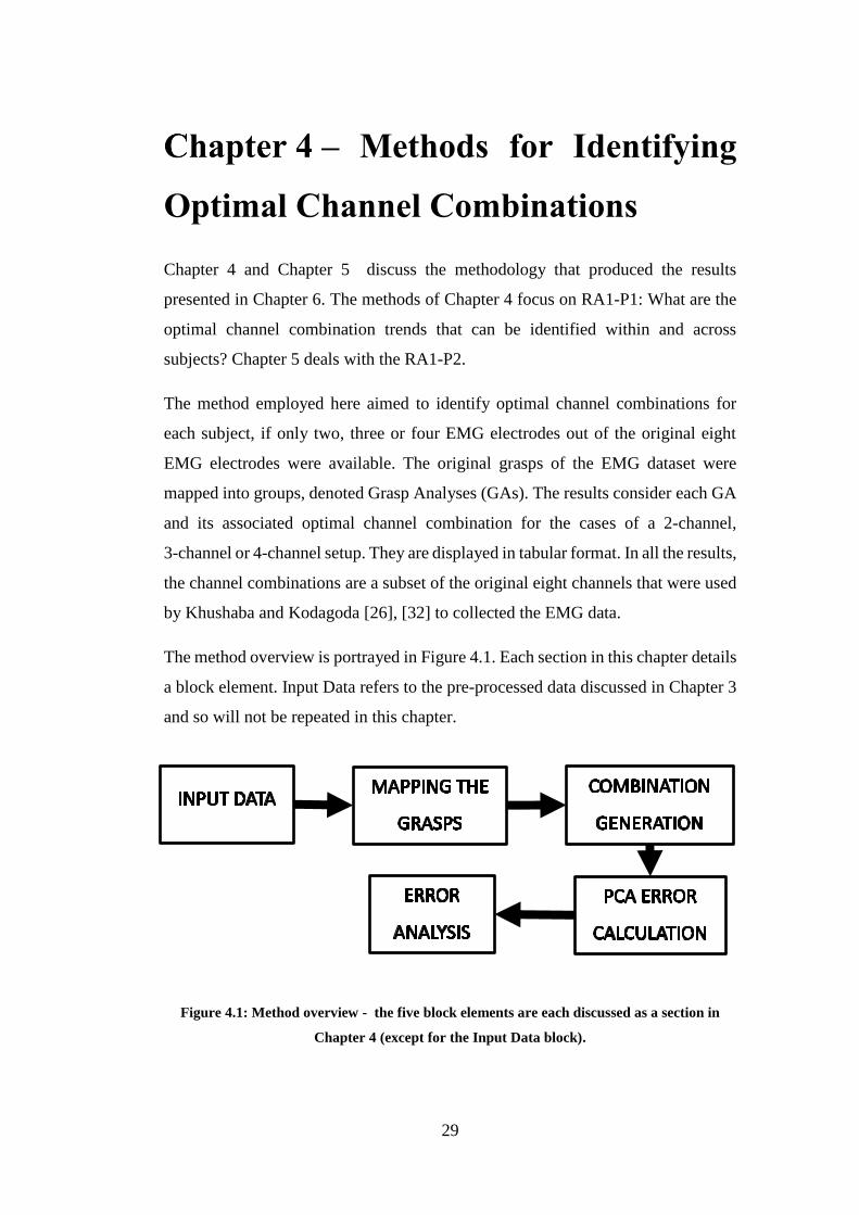
The method overview is portrayed in Figure 4.1. Each section in this chapter details

a block element. Input Data refers to the pre-processed data discussed in Chapter 3

and so will not be repeated in this chapter.

Figure 4.1: Method overview - the five block elements are each discussed as a section in

Chapter 4 (except for the Input Data block).

30

Mapping the Grasps

A total of fifteen different grasps for each subject were investigated by the dataset

providers Khushaba and Kodagoda [26], [32] as discussed previously in Chapter 3.

Each of these grasps includes data for the eight channels that were placed around

the forearm of the subject during the data collection process. Each subject has three

trials for each grasp. To reduce the number of signals to analyse and reduce noise

in the signals, the current study averaged the three trials on a channel-by-channel

basis. To provide an analysis that was focussed on the EMG contributions for each

finger of the hand, the fifteen grasps were firstly grouped into three categories. The

three categories of GA are All Grasps, Single Grasp and Focal Grasp. Each

category has a specific pattern in terms of which grasps were used in a GA. All

Grasps considered all the grasps together, Single Grasp considered only the

individual finger grasps, and Focal Grasp included all the grasps related to the

“focal finger”. Table 4.1 summarizes this mapping.

The All Grasps category contains a single GA – All Grasps - which encompasses

all the grasps together. This GA would typically be done to identify the optimal

channel combination in a straightforward manner when it comes to training a

classification system. Since the All Grasps category obviously includes grasps that

are present in the other GAs, often the All Grasps GA yielded similar optimal

channel combinations to some of the other GAs, though this was not always the

case. The All Grasps GA was overall considered to be the best determinant for

identifying the optimal channel combinations, since it includes all the grasps. The

other GAs served to confirm this as well as provide insight into the more specific

channels that become more relevant with specific GAs.

The Single Grasp category of GAs contains only grasps that relate specifically to

the use of a single finger. Given that there are five grasps in the original fifteen that

meet this criterion, there are five GAs that map exactly from the grasps to the GAs.

These GAs were used to identify which channels are important for each individual

finger, and these important channels were expected to be different for the different

fingers. There were cases where different GAs identify the same channels as being

important, most notably in the case of any combination of the middle, ring and little

31

fingers, since these fingers tend to use muscles that are closely anatomically related.

These muscles are the FDS and FDP, which have been previously discussed in

Chapter 2. In such cases a single channel placed over these muscles would register

an EMG signal that is generated by either of them.

Table 4.1: Details on the different GA categories, the GAs and the grasps included.

GA

Category GA Name

Number of

Grasps in GA Grasps Included

All Grasps All Grasps 15

T, I, M, R, L, T-I, T-M, T-R, T-L,

I-M, M-R, R-L, I-M-R, M-R-L,

HC

Single Grasp

Thumb 1 T

Index 1 I

Middle 1 M

Ring 1 R

Little 1 L

Focal Grasp

Thumb Focal 6 T, T-I, T-M, T-R, T-L, HC

Index Focal 5 I, T-I, I-M, I-M-R, HC

Middle Focal 7 M, T-M, I-M, M-R, I-M-R, M-R-

L, HC

Ring Focal 7 R, T-R, M-R, R-L, I-M-R, M-R-

L, HC

Little Focal 5 L, T-L, R-L, M-R-L, HC

The Focal Grasp category contains all GAs that were defined for containing any

grasps that involved the use of the ‘focal finger’. The focus of these GAs was on

the impact that the ‘focal finger’ would have on the selection process when it came

to the optimal channel combination. In many cases the result for different GAs in

this category were expected to be similar, since there were grasps that were

common to multiple GAs. However, there were cases where a GA identified a

different set of optimal channels, and these differences were investigated.

32

Generation of Channel Combinations

To find the best channel combination for the 2-channel, 3-channel and 4-channel

setups, all possible combinations needed to be generated and compared. The limit

on the number of channels in each respective setup lead to the maximum number

of possible combinations indicated in Table 4.2. For example, for any GA, when

analysing the GA to find the best 2-channel setup, there were a total of 28

combinations of the channels 1 to 8 that needed be generated and analysed against

each other. These values are calculated using the binomial coefficient method, in

this case (82

) = 28, (83

) = 56 and (84

) = 70. In total there were 154 (28 + 56 + 70)

combinations generated across the three reduced-channel setups for a single GA.

Table 4.2: Number of possible combinations when using only two, three or four channels.

Number of Channels Number of Combinations

2 28

3 56

4 70

The data used in this study was collected over a twenty-second time period [26],

[32]. This total time was split into four smaller time periods (TPs): 0 – 5s, 5 – 10s,

10 – 15s and 15 – 20s. In addition to these smaller TPs, a full 0 – 20s TP was used

as a comparison marker when it came to analysing the combinations. The splitting

up of the TPs allowed for a more detailed analysis into how prevalent channel

combinations change with time. Each combination thus consisted of a group of five

TP sections.

In cases where a GA had multiple grasps associated with it, the relevant TPs from

each grasp were appended together to form the full amount of data required for the

analysis. For example, consider the Thumb Focal GA, which contained six grasps.

When generating the 2-channel combinations for this GA, the 0 – 5s TP for the

relevant channels for all six grasps were appended together, and this occurred in the

same order for each TP.

33

Once the combinations and TPs were generated, there were a total of 770 (28*5 +

56*5 + 70*5) channel combinations for a single GA, spanning the 2-channel,

3-channel and 4-channel setups.

Error Calculation

In order to find which channel combination best represented the 2-channel,

3-channel and 4-channel setups, three error metrics: NRMSE, CC, and MSC were

used, as reviewed in Chapter 2. These error metrics were applied to each of the

individual TPs within each combination. This allowed for comparisons between

similar TP’s in different combinations.

The original eight channels of data for the GA were used to compute the error

metrics. PCA was applied as an FEM, as described previously in Chapter 2. The

use of PCA generated an eight-by-eight covariance matrix along with its

eigenvalues and eigenvectors. The Eigenvectors are re-ordered according to the

eigenvalues, such that the columns represent the eight PCs of the data, in order from

highest to lowest variance values. A 2-PC model of the data was created by

retaining only the first two PCs from the 8-PC model. This 2-PC model was

reversed to give the reconstructed signals for the eight channels of data. Note that

PCA was not used as a dimensionality reduction technique in this case.

The 2-PC model enabled a comparison between the eight original channels and

eight reconstructed channels. Each channel of the 8-PC and 2-PC models was

compared using the NRMSE, CC and MSC error metrics. These three values

represent the correlation between the two models for each channel. To calculate the

error metric values for a particular combination (which includes either two, three

or four channels), the error values for all the channels included in the combination

were averaged. This gave three error metrics that represented each combination.

This process was performed for each of the TPs, so each channel combination had

three error metrics that represent each of its five TPs.

The reason that the 8-PC model and the 2-PC model were compared to each other

was due to signal variance bias. When a particular muscle contracts, the channel

34

that is measuring that muscle has an increased amplitude. This can be seen in a PCA

as a larger variance when compared to non-active channels. Performing PCA and

retaining only the first two PCs meant that once the channel signals were

reconstructed, the channels that were actively measuring contraction had lower

error values (since PCA retains variance) which is equivalent to a larger amplitude.

Thus, when comparing the 8-PC model with the 2-PC model using the error metrics,

the active channels within the combination of channels were determined according

to least overall error.

Error Analysis

For each of the three channel setups, all possible combinations were generated, each

combination consisting of five TPs, and each TP being represented by three error

metrics. These error metrics were compared to identify a single best channel

combination for each of the 2-channel, 3-channel and 4-channel setups. This was

done in two stages:

In the first stage the error metrics for the same TPs across combinations were

compared, and a best channel combination was identified for each of the five TPs.

This reduces the 770 (28*5 + 56*5 + 70*5) combinations to 15 (5 + 5 + 5). For

example, in the 2-channel setup, the 28 combinations are compared on a TP-to-TP

basis, and only a single channel combination is identified for each TP. The error

metrics for the channel combinations were compared using the following rules:

1) The channel combination with the lowest NRMSE, highest CC and highest

MSC was chosen from all the combinations.

2) This optimal channel combination’s error metrics were compared to the

average of all the error metrics to ensure that they are lower than the

average, since if the best error values were not better than the total average,

then there was a mistake in the selection of the optimal channel

combination.

3) There were cases where the three error metrics did not all agree on what the

optimal channel combination was. In these cases, the combination that

35

showed the best two out of the three metrics was selected as the optimal

channel combination.

4) There were cases where none of the three error metrics agreed on what the

optimal channel combination was. Since the three error metrics were given

the same weight, such a result was completely inconclusive.

Upon completion of this process, each channel setup had five channel combinations

(one for each TP), or in very rare cases there was no outcome.

In the second stage, all channel combinations within either the 2-channel, 3-channel

or 4-channel setups, for the different TPs, were compared to each other. This

identified the overall best combination through all the TPs, giving a single optimal

channel combination for each of the 2-channel, 3-channel and 4-channel setups. In

the majority of cases the channel combinations remained consistent throughout the

different TPs, and were confirmed by the 0 – 20s TP. In cases where this did not

occur however, a single optimal channel combination was identified. A sequence

of steps was followed when comparing the optimal channel combinations from the

different TPs to each other. This sequence was followed until an outcome was

reached, and is as follows:

1) Considering all four of the TPs (excluding the 0-20s TP), select the most

common channel combination.

2) If there is no clear optimal channel combination, include the 0-20 s TP as

well.

3) If there is still no clear optimal channel combination, weight the

combinations to favour those that were determined to be the optimal channel

combination in their TP with confirmation of all three error metrics (as

opposed to only two of the error metrics).

4) If there is still no clear optimal channel combination, choose the 0-20 s TP

combination as the optimal channel combination.

5) If there is no 0-20 s TP optimal channel combination (due to being

inconclusive), choose the combination that has the highest variance data

content.

36

6) If all the TP combinations are inconclusive (none of them were confirmed

by two or three error metrics), the channel combination is considered

completely inconclusive, and this is indicated.

The sequences identified a single optimal channel combination for each of the

2-channel, 3-channel and 4-channel setups. It tended to show a progression of what

channel was added when going from the 2-channel setup to the 3-channel setup for

example.

This two-stage process was repeated for each GA, generating for each subject the

table described at the beginning of Chapter 4 and seen in Chapter 6.

Chapter Summary

This chapter described the methodology for identifying the optimal channel

combination for each GA, for the 2-channel, 3-channel and 4-channel setups. The

described process yielded results for all eleven GAs for each subject.

37

– Methods for Graphical

Representation of Results

Chapter 4 focussed on identifying the optimal channel combinations for the

2-channel, 3-channel and 4-channel setups for each GA, for each subject to answer

RA1-P1. This chapter discusses the methodology that could answer RA1-P2: How

much impact does the reduction in the number of electrodes have on the variance

content of the data? These results serve as a quality evaluation, where the

reduced-channel setups can be compared directly to their baseline eight-channel

setup counterparts.

This quantitative analysis employed the variance of PCA as a metric for the

information content retained in the reduced-channel combinations. For each All

Grasps optimal channel combination, the percentage of variance retained (PVR) by

the reduced-channel setup was calculated. These percentages are presented in a

graphical form in Chapter 6 that allows for comparison when different numbers of

channels, as well as the different TPs are considered.

PCA employs variance to indicate which dimensions of a dataset are important, and

this principle was applied to provide a measure indicating which channels are

important: The PVR quantified the contribution that a channel had relative to the

total amount of variance for all channels measured together.

The computation of the PVR metric is detailed in Section 5.1.

Percentage of Variance Retained (PVR)

As discussed in Chapter 4 PCA involves the generation of an eight-by-eight

covariance matrix involving all the channels. This was done prior to identifying the

PCs. For each GA a covariance matrix for all eight channels was calculated, denoted

C. The trace of this covariance matrix sums all variances of all eight channels. This

value is a baseline variance content using all the electrodes which can be compared

to the reduced electrodes setup. The same procedure is followed to generate a

38

covariance matrix for only the optimal reduced channel combinations, denoted B.

The trace of B reflects the total amount of variance when only using the optimal

channels. A PVR is defined as the ratio between the two traces:

𝑃𝑉𝑅 =𝑡𝑟𝑎𝑐𝑒 (𝐵)

𝑡𝑟𝑎𝑐𝑒 (𝐶)𝑥 100 (2)

This PVR calculation can be repeated for each TP within a channel combination,

thus allowing for the different TPs to be compared. The patterns of these

percentages were compared across different subjects, as well as between the Single

Grasp GAs and the Focal Grasp GAs. These results are discussed in Chapter 7.

Chapter Summary

Additional results were generated to supplement the tables generated in Chapter 4

and presented in Chapter 6 to provide an answer for RA1-P2: How much impact

does the reduction in the number of channels have on the variance content of the

data?

39

– Results

The results generated using the methodologies described in Chapter 4 and Chapter

5 are presented here. Each subject’s results are in the form of: 1) A table that shows

all optimal channel combinations for all the GAs that were investigated, for the

2-channel, 3-channel and 4-channel setups, and 2) A graph that shows the PVR for

the All Grasps GA. These are displayed in Sections 6.1 to 6.7. Note that for each

subject, only the most common optimal channel combinations are presented. This

follows the process outlined in Section 4.4., whereby the five TPs for each GA were

combined to get a single optimal channel combination.

Section 6.8 used the individual subject results to compile a table of the most

common optimal channel combinations for each subject for the 2-channel,

3-channel and 4-channel setups. These compiled results are compared in discussion

in Chapter 7.

Section 6.9 considers the averages of the PVRs for each subject across each of their

TPs, which were visualised for further discussion in Chapter 7.

40

Subject 1

The results of the optimal channel combinations for Subject 1 are shown in Table

6.1, followed by the PVR results of the All Grasps GA for the 2-channel, 3-channel

and 4-channel setups in Figure 6.1.

Table 6.1: Subject 1’s optimal channel combinations for the GAs.

GA Analysed Most Common Combination

Name Grasp count 2-channel 3-channel 4-channel

All 15 1 7 1 7 8 1 2 7 8

Thumb 1 1 6 1 5 6 1 5 6 8

Index Finger 1 1 6 1 2 6 1 2 6 8

Middle Finger 1 1 8 1 2 8 1 2 7 8

Ring Finger 1 1 5 1 2 5 1 2 5 8

Little Finger 1 1 4 1 4 5 1 4 5 8

Thumb Focal 6 1 7 1 7 8 1 2 7 8

Index Focal 5 1 7 1 7 8 1 2 7 8

Middle Focal 7 1 7 1 7 8 1 2 7 8

Ring Focal 7 5 7 5 6 7 5 6 7 8

Little Focal 5 1 7 1 7 8 1 2 7 8

Figure 6.1: Subject 1’s PVR for the All Grasps GA.

40

50

60

70

80

90

100

2-channel 3-channel 4-channel

VA

RIA

NC

E D

AT

A C

ON

TE

NT

(%

)

0-5s TP

5-10s TP

10-15s TP

15-20s TP

41

Subject 2


6.2, followed by the PVR of the All Grasps GA for the 2-channel, 3-channel and

4-channel setups in Figure 6.2.




All 15 5 8 4 5 8 3 4 5 8

Thumb 1 1 8 1 7 8 1 2 7 8

Index Finger 1 1 8 1 7 8 1 2 7 8

Middle Finger 1 1 8 1 2 8 1 2 7 8

Ring Finger 1 5 7 5 7 8 1 5 7 8

Little Finger 1 1 8 1 7 8 1 2 7 8

Thumb Focal 6 7 8 6 7 8 1 6 7 8

Index Focal 5 5 8 4 5 8 5 6 7 8

Middle Focal 7 5 8 1 5 8 None

Ring Focal 7 5 8 5 7 8 1 5 7 8

Little Focal 5 5 8 5 7 8 None


40

50

60

70

80

90

100


VA

RIA

NC

E D

AT

A C

ON

TE

NT

(%

)

0-5s TP

5-10s TP

10-15s TP

15-20s TP

42

Subject 3







All 15 7 8 1 7 8 1 6 7 8

Thumb 1 1 8 1 2 8 1 2 7 8

Index Finger 1 1 8 1 7 8 1 6 7 8

Middle Finger 1 1 8 1 7 8 1 2 7 8

Ring Finger 1 1 6 1 6 8 1 2 6 8

Little Finger 1 1 8 1 2 8 1 2 7 8

Thumb Focal 6 7 8 1 7 8 1 6 7 8

Index Focal 5 7 8 1 7 8 1 6 7 8

Middle Focal 7 7 8 1 7 8 1 6 7 8

Ring Focal 7 7 8 1 7 8 1 6 7 8

Little Focal 5 7 8 1 7 8 1 6 7 8


40

50

60

70

80

90

100


VA

RIA

NC

E D

AT

A C

ON

TE

NT

(%

)

0-5s TP

5-10s TP

10-15s TP

15-20s TP

43

Subject 4







All 15 5 6 5 6 7 3 4 5 6

Thumb 1 5 6 3 5 6 1 2 6 8

Index Finger 1 5 6 4 5 6 4 5 6 7

Middle Finger 1 5 6 4 5 6 4 5 6 7

Ring Finger 1 5 6 5 6 7 4 5 6 7

Little Finger 1 5 6 1 5 6 1 4 5 6

Thumb Focal 6 1 7 1 7 8 1 2 7 8

Index Focal 5 6 7 5 6 7 4 5 6 7

Middle Focal 7 6 7 5 6 7 3 5 6 7

Ring Focal 7 6 7 5 6 7 None

Little Focal 5 6 7 5 6 7 5 6 7 8


40

50

60

70

80

90

100


VA

RIA

NC

E D

AT

A C

ON

TE

NT

(%

)

0-5s TP

5-10s TP

10-15s TP

15-20s TP

44

Subject 5







All 15 1 5 1 2 5 1 2 5 8

Thumb 1 1 6 1 5 6 1 5 6 8

Index Finger 1 1 6 1 2 6 1 2 4 6

Middle Finger 1 1 5 1 5 6 1 5 6 8

Ring Finger 1 1 5 1 5 6 1 2 5 6

Little Finger 1 1 6 1 5 6 1 2 5 6

Thumb Focal 6 1 5 1 2 5 1 2 5 8

Index Focal 5 1 5 1 2 5 1 2 4 5

Middle Focal 7 1 5 1 5 8 1 4 5 8

Ring Focal 7 1 5 1 5 8 1 2 5 8

Little Focal 5 1 5 1 2 5 1 2 5 8


40

50

60

70

80

90

100


VA

RIA

NC

E D

AT

A C

ON

TE

NT

(%

)

0-5s TP

5-10s TP

10-15s TP

15-20s TP

45

Subject 7







All 15 1 5 1 2 5 1 2 5 8

Thumb 1 1 8 1 7 8 1 2 7 8

Index Finger 1 1 8 1 7 8 1 2 7 8

Middle Finger 1 1 8 1 2 8 1 2 7 8

Ring Finger 1 5 8 1 5 8 1 5 7 8

Little Finger 1 1 5 1 2 5 1 2 5 6

Thumb Focal 6 1 5 1 2 5 1 2 5 8

Index Focal 5 1 5 1 5 8 1 2 5 8

Middle Focal 7 5 7 5 7 8 1 5 7 8

Ring Focal 7 5 7 5 7 8 5 6 7 8

Little Focal 5 5 7 5 7 8 1 5 7 8


40

50

60

70

80

90

100


VA

RIA

NC

E D

AT

A C

ON

TE

NT

(%

)

0-5s TP

5-10s TP

10-15s TP

15-20s TP

46

Subject 8







All 15 1 5 1 5 6 1 5 6 7

Thumb 1 1 2 1 2 8 1 2 3 8

Index Finger 1 1 8 1 7 8 1 2 7 8

Middle Finger 1 1 2 1 2 3 1 2 3 8

Ring Finger 1 1 5 1 5 6 1 2 5 6

Little Finger 1 1 2 1 2 8 1 2 3 8

Thumb Focal 6 1 5 1 5 6 1 5 6 7

Index Focal 5 1 6 1 6 7 1 5 6 7

Middle Focal 7 1 6 1 5 6 1 5 6 7

Ring Focal 7 5 8 5 6 8 5 6 7 8

Little Focal 5 1 5 1 5 6 1 5 6 7


40

50

60

70

80

90

100


VA

RIA

NC

E D

AT

A C

ON

TE

NT

(%

)

0-5s TP

5-10s TP

10-15s TP

15-20s TP

47

Most Common Channel Combinations

The overall most common channel combinations for the 2-channel, 3-channel and

4-channel setups for each subject are presented in Table 6.8.

In identifying the most common channel combinations for each subject, the results

for the GAs were weighted. The All Grasps GA was given a weighting of value

three, the Focal Grasp GAs were each given a weighting of value two, and the

Single Grasp GAs were each given a weighting value of one. These weightings

were assigned according to the number of grasps in the GAs; the All Grasps GA

has 15 grasps, the Focal Grasp GAs have between five and seven grasps, and the

Single Grasp GAs have a single grasp each.

This was done to give more weight to the GAs that included more grasps, since

these GAs found optimal channel combinations under more complex circumstances

(the inclusion of multiple grasps into the analysis as opposed to a single grasp). It

is noted that each of the Focal Grasp and Single Grasp GA categories have five

GAs each; and the All Grasps GA only has one. The score for the All Groups GA

was kept at three to avoid over-fitting the optimal channel combination to a single

result.

Table 6.8: Overall most common channels for each subject for the 2-channel, 3-channel and

4-channel setups.

Subject Number Most common channel combinations

2-channel setup 3-channel setup 4-channel setup

1 1 7 1 7 8 1 2 7 8

2 5 8 5 7 8 1 2 7 8

3 7 8 1 7 8 1 6 7 8

4 5 6 5 6 7 4 5 6 7

5 1 5 1 2 5 1 2 5 8

7 1 5 1 2 5 1 2 5 8

8 1 5 1 5 6 1 5 6 7

48

The optimal channel combination for each reduced-channel setup with the highest

score was identified and presented. This analysis did not yield any pattern for 3 out

of the 231 (33*7) results, a total of 1.3%, which were not considered further in this

study.

Average Percentage Variance Retained

As described in Chapter 5 the results for the PVRs for each TP were calculated

using the identified optimal channel combinations for the All Grasps GA for each

subject. These results were displayed in a graph for each subject, showing the

progression of TPs. Table 6.9 displays the average PVR of all TPs for each channel

setup for each subject. These results are presented graphically in Figure 6.8.

Table 6.9: PVR by each subject for the All Grasps optimal channel combinations, for the

2-channel, 3-channel and 4-channel setups.

Subject Variance Data Content (%)


1 57.1 70.9 74.5

2 62.5 62.8 63.1

3 60.1 78.1 87.5

4 58.4 74.9 59.1

5 84.9 86.0 88.9

7 67.2 73.7 83.2

8 61.4 70.7 79.2

49

Figure 6.8: Average PVR for each subject for each channel combination (coloured lines),

including the average for all subjects (black line).

Chapter Summary

This chapter presented the results obtained using the methods described in Chapter

4 and Chapter 5. Results for each of the seven subjects were presented and were

followed by results summarising the overall most common optimal channel

combinations, as well as the average PVR, across all subjects. The main findings

of this study could be better observed and discussed by looking at the results across

all subjects, as opposed to on a subject-by-subject basis. These latter results will be

discussed in Chapter 7.

50

55

60

65

70

75

80

85

90


Per

cen

tage

of

Var

ian

ce R

etai

ned

(%

)

Subject 1

Subject 2

Subject 3

Subject 4

Subject 5

Subject 7

Subject 8

Average

50

– Discussion

This chapter discusses the derived results presented Table 6.8, Table 6.9 and Figure

6.8, in Chapter 6. The insights gained from these results are presented, with the aim

of using them to answer the RQ.

Section 7.1 covers the proposed EMG electrode placement and muscle associations

that the current study uses as a basis for discussion. These were based on the study

where the data was originally collected by Khushaba and Kodagoda [26], and the

proposed placements by Naik et al. [61] discussed in Chapter 3.

Section 7.2 discusses the optimal channel combinations for the 2-channel setup.

Following this, the 3-channel setup is discussed in Section 7.3, and lastly the 4-

channel setup is discussed in Section 7.4. A number of conclusions are made in

each section. These were used to answer RQ and related research goals.

Section 7.5 discusses the PVR trends and identifies some important results that are

used to help answer the RQ and associated research goals.

Lastly, Section 7.6 combines the discussions and results of the previous sections to

answer the RQ proposed in Chapter 1. This is done through systematically dealing

with each goal: RA1-P1, RA1-P2, RA1 and RA2 and their relations to each other.

Updated Electrode Placements on the Forearm

The proposed electrode placements used in this study were based on the electrode

placement proposed by Naik et al. [61], which were themselves based on the

placements in the Khushaba and Kodagoda [26]. These placements were marked

on anatomical diagrams from Chapter 2 such that the association between the

electrodes and muscles can be identified, as shown in Figure 7.1, Figure 7.2 and

Figure 7.3. Following this, the active underlying muscles (if they are below the

surface muscles) are identified and their associations mapped, as shown in Table

7.1.

51

Figure 7.1: Anterior surface view of the right forearm, showing the electrode placements

(numbered red circles) and FDS (blue) (Adapted from [58]).

Figure 7.2: Anterior deep view of the right forearm, showing the same electrode placements

as in Figure 7.1 (numbered red circles). Seen here are the FPL (green), FDP-L (orange) and

FDP-M (blue) (Adapted from [59]).

Figure 7.3: Posterior surface view of the right forearm, showing the electrodes placements

(numbered red circles). Seen here are ECRL (blue), ED (red), ECU (green), ECRB (orange),

EPL (purple), APL (light green) and EPB (light blue) (Adapted from [60]).

1

2

8

7

2

3

4

5

6

2

3

4

56

52

Table 7.1: Muscle-electrode associations used in the current study, including the deeper

active muscles.

Surface Muscle Electrode(s) Active Muscles (might be deeper

to the surface muscle)

ED 1 ED

Brachioradialis 2, 3 FPL

Supinator 4 FDS, FPL, FDP-L

FCR 5 FDS, FDP-L, FDP-M

FCU 6, 7 FDP-M

ECU 8 ECU

These associations assist the discussion on the results of Chapter 6 with respect to

the optimal electrode placements that were identified, and the associated muscles

involved. Although the exact placement of the electrodes in the original Khushaba

and Kodagoda study could not be verified [26], the current study provides

correspondence between EMG electrodes and muscles which may give some

indication on the relative importance of the various muscles in the grasps. This

avoids the traditional assumption that an electrode placed directly over a specific

muscle will always yield and acceptable-quality EMG signal.

The region near electrodes 5, 6 and 7 is commonly referred to as the common flexor

tendon, where some of the anterior surface muscles, including non-marked muscles

FCR and FCU attach. Although these muscles are not directly involved in the hand

grasps as discussed in Chapter 2, the common attachment at the common flexor

tendon may in some cases cause electrodes 6 and 7 to record additional EMG

signals that may be generated by other muscles.

Additionally, Naik et al. [61] consider electrodes 1, 2, 7 and 8 to be located on the

posterior aspect of the forearm, with electrodes 3, 4, 5 and 6 on the anterior aspect.

The current study proposes that electrode 7 is a part of the anterior electrodes, where

only electrodes 1, 2 and 8 are located posteriorly, and electrodes 3, 4, 5, 6 and 7 are

located anteriorly. Even though channel 2 is a posterior channel, its unique location

means that it might still be activated when the thumb is flexed, which requires the

FPL muscle.

53

2-Channel Setup Trends

When considering the 2-channel setup in Table 6.8, it becomes clear that there is a

posterior channel and an anterior channel for each subject, except for Subject 4,

where there are two anterior channels present. The deviation from the trend for

Subject 4 will be addressed at multiple points in the discussions to follow.

In terms of the posterior channels, channels 1 and 8 correspond to the ED and ECU

muscles respectively. The presence of these channels in the optimal combinations

could initially be questioned, since the grasps under investigation are only

concerned with finger flexion, not extension. However, the inclusion of these

channels can be explained by the positioning of the non-active fingers when a single

or group of fingers is flexed. The grasp images in Chapter 3 show that when

performing any grasp, the non-active fingers are not relaxed, but are rather extended

to be held straight. The extension is achieved by activating the ED muscle, hence

the inclusion of channel 1.

Channel 8 is located next to channel 1 on the posterior forearm. It is normally

associated with the ECU muscle as seen in Figure 7.3. The ECU muscle should

only be active when all the fingers are closed together (as indicated in Table 2.1),

so would not be considered very commonly active. There are two possible reasons

why channel 8 is seen actively: 1) The nature of EMG electrode placements

(because of differences in the anatomy of subjects) can cause electrodes to be

shifted from their noted positions. In this case, channel 8 is measuring the activity

of the ED muscle, not the ECU muscle. 2) The EMG signals measured by the

electrodes is often a combination of EMG generated by multiple different muscles,

not only the muscle the electrode is placed over. In this case, channel 8 may be

placed correctly, but is still measuring the cross-talk from the ED muscle due to its

proximity.

The anterior channels in the 2-channel setup are channels 5, 6 and 7. These channels

correspond to the FDS, FDP-L and FDP-M muscles. Their presence is expected,

since the muscles correspond directly to the flexion of the fingers, and these

54

muscles are associated with the common flexor tendon, where these muscles are

attached.

The 2-channel combination of Subject 4 has a different pattern compared to the

other subjects. In this case channels 5 and 6 are present, corresponding to the FDS

and FDP muscles. The presence of these channels is not surprising. The lack of

presence of any posterior channels could to be due to a lack of co-contraction by

the ED muscle of this subject during testing. This presents an issue, since an optimal

channel selection needs to account for the flexion of the fingers during contraction,

as well as the extension of the fingers to return the hand to rest.

There are a few conclusions that can be drawn from the 2-channel setup. Firstly,

the combinations for each subject consist of an anterior channel (channel 5, 6 or 7)

and a posterior channel (channel 1 or 8), except in Subject 4’s case. Due to this, the

channels for the subjects generally tend to be on opposite sides of the forearm to

maximise EMG data collection. This is not the case for Subject 4, since channels 5

and 6 are directly next to each other on the anterior side of the forearm. Secondly,

posterior channels 1 (over ED) and 8 (over ECU) are confirmed as important by

Khushaba and Kodagoda [26], as well as Naik et al. [61]. Khushaba and Kodagoda

[26] generally suggest that these muscles may be relevant, and Naik et al. [61]

specifically discusses the importance of ED and ECU as a part of their Simple

Finger Movements results.


The 3-channel setups from Table 6.8 follow on from the 2-channel setups. For each

subject, an additional channel is added to the channels presented in the 2-channel

setup. This progression is important to note, since if channels are identified as

important for the strictest optimisation process (2-channel setup), then they should

appear in the 3-channel and 4-channel setups.

The channel added from the 2-channel to 3-channel setup is not the same for each

subject. Although the subjects are consistent in terms of adding a channel to the

channels seen in the 2-channel setup, these additional channels are not the same for

55

each subject. This indicates that there is some inter-subject variance, which is

expected for an optimisation process such as this, since the subjects’ all have

differing muscle profiles.

The exact combinations in the 3-channel setups might be different across subjects,

but trends can still be identified. With the addition of a third channel, some

identifiable subject sub-groups can be seen. Subjects 1, 2 and 3 show a disposition

towards including channels 7 and 8, with some variation on the third channel

(denoted group 1). Subjects 5, 7 and 8 select for channels 1 and 5, again with some

variation on the third channel (denoted group 2). Note the presence of a posterior

channel and an anterior channel when identifying these sub-groups. Subject 4

continues to show a deviation from the other subjects when considering the

3-channel setup. Even though this is the case, Subject 4 remains consistent in the

addition of a channel (channel 7) to the channels present in the 2-channel setup

(channels 5 and 6), but this additional channel is also an anterior channel. This

further supported the idea that there was no finger extension during testing.

An additional posterior channel was added for Subjects 1, 3, 5 and 7. Channel 2 is

the new type of channel that is seen in the 3-channel setup, and its unique location

(lying over FPL) indicates that its inclusion is due to the flexion actions of the

thumb.

An additional anterior channel was added for Subjects 2, 4 and 8. The anterior

channels show more consistency than the posterior channels in terms of location.

All the anterior channels (channels 5, 6 and 7) are located around the common

flexor tendon, corresponding to the FDS, FDP-L and FDP-M muscles. This

indicates that the grasps that tend to give a higher EMG reading are those were

multiple muscles are involved at the same time.

When Andrews [41] and Andrews et al. [17] considered a multiple-finger typing

task, the FDP and ED muscles are identified as being most commonly selected for

when using two channels. Extending this result to four channels showed selection

for electrode placements over FDS, FDP, ED and ECU. In the current study

channels 5, 6 (and 7), 1 and 8 correspond to these muscles.

56


The 4-channel setups from Table 6.8 follow on from the 3-channel setups. As

discussed previously, an additional optimal channel is added to the previously

optimally-selected channels in the 3-channel setup. This occurs in all subjects

except Subject 2, where channels 1 and 2 are added, and channel 5 is removed from

the combination.

As before, the inter-subject variation is evidenced by the difference in optimal

channel combinations for the different subjects. The two subject sub-groups

identified previously in Section 7.3, namely group 1 (channels 7, 8 and a variable

channel)) and group 2 (channel 1, 5 and a variable channel) can be extended to

include an additional channel. Channel 1 can be added group 1, so it includes

channels 1, 7, 8 and a variable fourth channel. Channel 2 can be added to group 2,

so it includes channels 1, 2, 5 and a variable fourth channel.

Similarly to the previous case, there is variation on the fourth channel within the

sub-groups. The sub-groups display some interesting trends, even though overall

the channel combinations are converging. The electrodes for group 1 (channels 1,

7 and 8) are all located in a focussed area on the forearm. This contrasts the

placements of the electrodes for group 2 (channels 1, 2 and 5), where the electrodes

are placed in a dispersed fashion. This indicates that there is no particular pattern to

the groupings of channels.

As channels have been added, in terms of posterior channels channel 2 has become

much more common. Its unique location influences the inclusion of it. It is

interesting to note that there are many GAs that include some form of thumb grasp

(whether multiple-finger or single-finger). Due to this, it was expected that channel

2 would become more common in either the 2-channel or 3-channel setups.

However, as evidenced, the contributions from the other GAs outweighed channel

2 until the 4-channel setup. This is potentially due to the combined contraction

strength of the other fingers that was stronger than the thumb. This meant that the

optimal channels selected for were focussed around these muscles.

57

Subject 4 is an outlier for the 4-channel setup as well, when comparing their channel

combinations to the other subjects. As mentioned previously, the possible reason

for this could be a lack of co-contraction of non-active fingers during the EMG data

collection process. However, only identifying anterior optimal channels in only one

subject might indicate a form of data corruption that was not identified during the

visual screening process.

When considering the 2-channel, 3-channel and 4-channel setups together, some of

the more notable channels are 1, 2, 5, 6, 7 and 8. These are shown in Figure 7.4,

Figure 7.5 and Figure 7.6. These notable channels correspond to the following

active muscles: ED, FPL, FDS/FDP-L/FDP-M (common flexor tendon), and ECU.

Channel 2 was a notable inclusion, for the fact that it was not relevant in the 2-

channel context and not as commonly seen as the other channels in the 3-channel

setup. Its inclusion is crucial, since it accounts for the flexion activity of the thumb.

As previously mentioned, some of these muscles were also identified as important

by the dataset authors, Khushaba and Kodagoda [26]. Their conclusions were that

the surface muscles ED, ECU, and FCU (which lies over the active muscle FDP)

were relevant, even though their conclusions about what these muscles represent

was somewhat limited in scope.

These differences in optimal channel combinations mean that the process of

identifying optimal electrode placements is heavily subject-dependent. This is

similar to a finding by Andrews et al. [17]. The important channels identified in

this study can most certainly reduce the number of EMG electrode placements

required. However, in some cases these electrode placements should be considered

a preliminary starting point. Should the EMG data not be of sufficient quality,

further testing of electrode placements may be necessary.

58

Figure 7.4: Anterior deep view of the right forearm, highlighting the notable channels in

yellow (Adapted from [59]).

Figure 7.5: Anterior surface view of the right forearm, highlighting the notable channels in


Figure 7.6: Posterior surface view of the right forearm, highlighting the notable channels in


Percentage Variance Retained Trends

The average PVR for each subject for the 2-channel, 3-channel and 4-channel

setups increase as the number of available channels increased, as illustrated in Table

6.9 and in Figure 6.8. This can be expected since more information is available for

processing as the number of channels increase. Subject 4 was the exception to this

rule, where the average PVR in the 4-channel setup was lower than the 3-channel

1

2

8

7

2

3

4

5

6

2

3

4

56

59

setup. This could potentially be due to the selection of only anterior channels for

the optimal 2-channel, 3-channel and 4-channel combinations.

Subject 5 displayed the highest consistent PVR for all the channel setups. In this

case, the reduction in the number of channels to two still yielded a PVR of 84.9%.

Subject 3 had the most significant change in PVR, increasing from 60.1% in the

2-channel setup to 87.5% in the 4-channel setup. There doesn’t appear to be any

correlation between the optimal channels in the 2-channel, 3-channel and 4-channel

setups for these two well-performing subjects. Subject 3 was part of group 1 in

terms of channel sub-groups, and Subject 5 was part of group 2. Even if a

connection cannot be found between these sub-groups, it can be concluded that

neither sub-grouping of channels is superior to the other. Thus, the problem of EMG

electrode placement remains a subject-dependent task.

Subjects 2 and 4 showed unique results in terms of their PVR values. Subject 2’s

PVR was similar for all combinations at 62.5% for the 2-channel, 62.8% for the

3-channel and 63.1% for the 4-channel setups. Subject 4’s PVR curve didn’t

increase from the 3-channel setup to the 4-channel setup, but rather decreased

sharply. The potential reasons for these outlier cases can be attributed to the

different patterns in the channel combinations for these subjects. In Subject 2’s

case, the loss of channel 5 in the 4-channel setup indicates that the channel

combinations for the GAs were not converging. In Subject 4’s case, the lack of a

posterior channel present in the 4-channel setup could be the reason that the PVR

was lower than in the 3-channel setup. It is not known why this is the case.

Apart from these two subjects, the PVR results support the assumption that this

dataset can be optimised for a reduced number of electrodes. For the seven subjects

used in this study, the minimum 2-channel setup PVR was 57.1% (Subject 1). The

minimum 3-channel setup PVR was 62.8% (Subject 2), and the minimum 4-channel

setup PVR was 59.1% (Subject 4). If the results for Subjects 2 and 4 are omitted

due to their deviation from the trends, the minimum 2-channel setup PVR was

57.1% (Subject 1), the minimum 3-channel PVR was 70.7% (Subject 8) and the

minimum 4-channel setup PVR was 74.5% (Subject 1).

60

Answering the Research Question

As described in Chapter 1 this study was segmented into various components. Each

component will repeat the relevant question then answer the component. To answer

the RQ, the components are answered in the following order: RA1-P1, RA1-P2,

RA1, RA2, and finally the RQ.

Research Aim 1 – Part 1

What are the optimal channel combination trends that can be identified within and

across subjects? Table 6.8 presents the most common optimal channel

combinations for each subject. In addition to the individual trends noted for each

subject, overall the most common channels are channels 1, 2, 5, 6, 7 and 8.

Research Aim 1 – Part 2

How much impact does the reduction in the number of electrodes have on the

variance content of the data? Table 6.9 and Figure 6.8 show the impact of using

limited numbers of EMG electrodes to collect data. With the minimum number of

channels considered in this study (2-channel setup), the minimum PVR was 57.1%.

The PVR improved to a minimum of 74.5% in the 4-channel setup, excluding the

results of the problematic Subjects 2 and 4.

Research Aim 1

What are the optimal two, three and four channel combinations for each subject

within the dataset, and how good is it compared to the original eight-channel dataset

for each subject? This component of the study is answered by RA1-P1 and RA1-P2.

Research Aim 2

Given the two, three and four channel optimal combinations identified in RA1,

which muscles are mainly responsible for generating this EMG data? Overall the

most common channels are channels 1, 2, 5, 6, 7 and 8. The channels correspond to

the following active muscles: ED, FPL, FDS, FDP-L, FDP-M (which make up the

common flexor tendon), and ECU.

61

Research Question

In using an eight-channel EMG dataset, what are the optimal combinations of two,

three and four EMG channels that consider the reduction in number of electrodes

and their variance data content when compared to the original eight-channel

dataset? As discussed previously, the optimal channel combinations for each

subject vary, but overall the most common channels have been identified for the

2-channel, 3-channel and 4-channel setups for each subject, as well as the overall

dominant channels being channels 1, 2, 5, 6, 7, and 8. The use of the optimal

channel combinations for each subject gives a 2-channel PVR range of

57.1 – 84.9% a 3-channel PVR range of 70.7 – 86.0% and a 4-channel PVR range

of 74.5 – 88.9%, when omitting the results for Subjects 2 and 4.

Future Work

The current study developed an algorithm that worked on the data that was used.

This implies that it will work on future datasets of a similar format as well. An

algorithm was developed as a proof-of-concept, but additional work needs to be

done to further develop and validate the algorithm. Discussed here are a number of

aspects that would benefit from additional work.

Future datasets that use the algorithm could benefit from using more electrodes (for

example 16 electrodes). These 16 electrodes could be set up in different

configurations, either in a single band around the forearm, or multiple bands at

different levels of the forearm. This effectively gives the algorithm more data to

work with to find optimal channel combinations.

Additional movements can also be added to the dataset, such as wrist movements.

Previous work by Eisenberg et al. [62] identified that EMG data generated by wrist

movements can be similar EMG generated by finger movements, and it would be

important to be able to differentiate between the wrist and finger movements.

This study focussed on the amount of PVR that was maintained by the optimal

channel combinations, but an aspect of PVR that would need to be investigated in

future would be the threshold amount of PVR that is considered to be acceptable.

62

This would be very dependent on the context of the application. In general, once

classification algorithms reach accuracies of more than 75% they start being

considered “useful”. The same could apply to the PVR in this study. It would

require substantial additional work to be able to conclude at what PVR there is

enough data variance for use in further processing, such as training classification

algorithms.

Lastly, the three error metrics (NRMSE, CC, and MSC) used to identify the optimal

channel combinations were given an equal weighting when it came to using them

to identify optimal channel combinations. Future work would involve identifying

which of these metrics may be more important or relevant than the others; or which

other error metrics could be used to better find optimal channel combinations.

Chapter Summary

This chapter aimed to answer the research goals of the RQ identified in Chapter 1.

This was done using discussion into the results presented in Chapter 6 and there

were some important insights that were gained in the process of answering these

research goals, as well as the RQ.

The 2-channel, 3-channel and 4-channel setups were discussed, and each provided

more insight into the trends that were shown in the results. For instance, the

common presence of channel 1 (located on the ED muscle) in optimal channel

combinations revealed that the extension of the fingers not actively involved in the

grasps was noticeable. This is important when it comes to collecting the EMG data,

and this should be accounted for when placing electrodes.

Given the insights gained, it was concluded that the subjects do show different

optimal channel combinations due to inter-subject variability, but channels 1, 2, 5,

6, 7 and 8 were the common across the subjects. These channels correspond

approximately to the ED, FDS, FDP and ECU muscles.

The PVR when using only select channels was discussed, and it was identified that

the PVR improved with the increase in number of electrodes. The reduction in

number of channels showed that a minimum PVR of more than 57% was seen when

63

using a 2-channel setup, more than 62% when using the 3-channel setup, and more

than 74% when using the 4-channel setup. These results do not include the PVRs

for Subjects 2 and 4, since their PVRs did not follow the trends identified.

These results and discussions were used to directly answer each of the identified

research goals, which were combined to answer the RQ proposed in Chapter 1.

Lastly, aspects of the study that are important to further explore in future work were

identified and discussed. These aspects were outside of the scope of the current

work, but are important to address.

64

– Conclusion

This chapter summarises the study, briefly covering the main points for each

chapter and their context with relation to the study goals.

Chapter 1 identified the need for trans-radial amputees to be able to perform their

ADLs using a prosthetic hand, where such a hand is controlled using EMG. To

effectively control a prosthetic hand using EMG, the placement and number of

electrodes needs to be optimised. Often this is done using the classification accuracy

of a classification algorithm as a metric for success, but this requires investigation

into the correct use of the classification algorithm as well. A requirement to

optimise the placement and number of EMG electrodes was identified, where the

solution doesn’t require a classification algorithm to be successful. To this end, an

RQ was identified, and split into a series of research goals. These focussed on the

optimal placement and number of EMG electrodes and the effects thereof when

using these optimal placements in a limited-channel context.

Chapter 2 considered the research on the optimisation of EMG electrodes on the

forearm, either by reducing the number of electrodes, or finding the best electrode

placements. All these studies make use of classification accuracy as the metric for

success. PCA is a method used to reduce the number of dimensions for

classification systems, but can also be used to reduce the dimensionality and

subsequently the quality of the data and compare the reduced-dimension model to

the original data. The reduced-dimension model can be used to identify important

EMG electrodes without the use of classification algorithms. To compare the

reduced model and the original data, three error metrics are defined: NRMSE, CC

and MSC. Additionally, the musculature of the forearm was reviewed in order to

derive optimal electrode placements.

Chapter 3 describes an 8-channel EMG dataset that was ideal for use in this study.

The subjects, hardware, software and testing procedures were outlined. This dataset

consisted of eight subjects. Each subject performed a series of fifteen grasps with

different combinations of fingers, and the EMG data was recorded using eight EMG

65

electrodes arranged around the forearm. Validations were performed to ensure the

quality of the dataset and note its limitations, as well as additional validations to

ensure that Matlab’s built-in PCARES function performed as expected.

Chapter 4 outlined the methodology to generate results that were used to answer

part of the research objectives. It discusses generating all possible combinations of

two, three and four channels of the original 8-channel EMG dataset. These

combinations are compared to the original 8-channel dataset using PCA. The

combination that showed the smallest error was identified as the optimal channel

combination for that number of electrodes. This process was repeated for each

subject for each of the defined GAs, to find an optimal channel combination for

each GA. These results were tabulated for each subject.

Chapter 5 complemented Chapter 4, using the optimal channel combinations

identified to find the variance data content that was retained from the original data

to see what impact the reduction in EMG electrodes had on the amount of variance

in the data. These results were shown in graphical format for each subject.

Chapter 6 presents the results generated in Chapter 4 and Chapter 5 for each subject.

These results are compiled for simpler discussion in Chapter 7.

Chapter 7 discusses the results obtained with a focus on the optimal channel

combinations for the 2-channel, 3-channel and 4-channel setups for the subjects.

The discussion identified channels 1, 2, 5, 6, 7 and 8 as being important in the

current study, which correspond approximately to the ED, FPL, FDS, FDP-L, FDP-

M and ECU muscles. The impact of reducing the number of EMG electrodes was

discussed, and it was seen that even when only using two of the channels, the PVR

was more than 57%. These results provided answers to the multiple research goals,

which led to answering the RQ in full. Potential future work on certain aspects of

the study were also outlined.

In terms of future work, the results obtained using a non-classification method for

optimisation of EMG electrode placement needs to be extended to different

datasets. The robustness of the methods should be tested on EMG datasets of

different data qualities, with different numbers of subjects. This ensures that

66

research making use of this method will not generate poor quality EMG data, that

could hamper further research efforts. To further extend the method, it can be

applied to more subjects, and subjects with different EMG datasets. This ensures

that the method is applicable to varying-application EMG datasets.

67

References

[1] Orthopaedic Trauma Institute, “Transradial Amputation - Orthopaedic

Trauma Institute (OTI),” Orthopaedic Trauma Institute (OTI). .

[2] C. Sollerman and A. Ejeskär, “Sollerman hand function test: a standardised

method and its use in tetraplegic patients,” Scand. J. Plast. Reconstr. Surg.

Hand Surg., vol. 29, no. 2, pp. 167–176, 1995.

[3] G. C. Matrone, C. Cipriani, E. L. Secco, G. Magenes, and M. C. Carrozza,

“Principal components analysis based control of a multi-dof underactuated

prosthetic hand,” J. NeuroEngineering Rehabil., vol. 7, p. 16, Apr. 2010.

[4] G. Magenes, F. Passaglia, and E. L. Secco, “A new approach of multi-d.o.f.

prosthetic control,” in 2008 30th Annual International Conference of the IEEE

Engineering in Medicine and Biology Society, 2008, pp. 3443–3446.

[5] A. Adewuyi, L. Hargrove, and T. Kuiken, “An Analysis of Intrinsic and

Extrinsic Hand Muscle EMG for Improved Pattern Recognition Control,”

IEEE Trans. Neural Syst. Rehabil. Eng., vol. PP, no. 99, pp. 1–1, 2015.

[6] M. Santello, M. Flanders, and J. F. Soechting, “Postural Hand Synergies for

Tool Use,” J. Neurosci., vol. 18, no. 23, pp. 10105–10115, Dec. 1998.

[7] J. R. Napier, “The Prehensile Movements of the Human Hand,” Bone Jt. J.,

vol. 38–B, no. 4, pp. 902–913, Nov. 1956.

[8] K. Englehart, B. Hudgins, P. A. Parker, and M. Stevenson, “Classification of

the myoelectric signal using time-frequency based representations,” Med.

Eng. Phys., vol. 21, no. 6–7, pp. 431–438, Jul. 1999.

[9] Y. Fang and H. Liu, “Robust sEMG electrodes configuration for pattern

recognition based prosthesis control,” in 2014 IEEE International Conference

on Systems, Man and Cybernetics (SMC), 2014, pp. 2210–2215.

[10] D. R. Merrill, J. Lockhart, P. R. Troyk, R. F. Weir, and D. L. Hankin,

“Development of an Implantable Myoelectric Sensor for Advanced Prosthesis

Control,” Artif. Organs, vol. 35, no. 3, pp. 249–252, Mar. 2011.

[11] T. R. Farrell and R. F. Weir, “Pilot comparison of surface vs. implanted EMG

for multifunctional prosthesis control,” in 9th International Conference on

Rehabilitation Robotics, 2005. ICORR 2005, 2005, pp. 277–280.

68

[12] E. Criswell, CRAM’s INTRODUCTION TO Surface Electromyography. Jones

and Bartlett Publishers.

[13] G. C. Matrone, C. Cipriani, M. C. Carrozza, and G. Magenes, “Real-time

myoelectric control of a multi-fingered hand prosthesis using principal

components analysis,” J. NeuroEngineering Rehabil., vol. 9, p. 40, Jun. 2012.

[14] P. Shenoy, K. J. Miller, B. Crawford, and R. P. N. Rao, “Online

Electromyographic Control of a Robotic Prosthesis,” IEEE Trans. Biomed.

Eng., vol. 55, no. 3, pp. 1128–1135, Mar. 2008.

[15] R. Kato, T. Fujita, H. Yokoi, and T. Arai, “Adaptable EMG Prosthetic Hand

using On-line Learning Method -Investigation of Mutual Adaptation between

Human and Adaptable Machine,” in The 15th IEEE International Symposium

on Robot and Human Interactive Communication, 2006. ROMAN 2006, 2006,

pp. 599–604.

[16] F. Tenore, A. Ramos, A. Fahmy, S. Acharya, R. Etienne-Cummings, and N.

V. Thakor, “Towards the Control of Individual Fingers of a Prosthetic Hand

Using Surface EMG Signals,” in 29th Annual International Conference of the

IEEE Engineering in Medicine and Biology Society, 2007. EMBS 2007, 2007,

pp. 6145–6148.

[17] A. Andrews, E. Morin, and L. McLean, “Optimal Electrode Configurations

for Finger Movement Classification using EMG,” in 2009 Annual

International Conference of the IEEE Engineering in Medicine and Biology

Society, 2009, pp. 2987–2990.

[18] A. d’Avella, “Decomposition of EMG patterns as combinations of time-

varying muscle synergies,” in First International IEEE EMBS Conference on

Neural Engineering, 2003. Conference Proceedings, 2003, pp. 55–58.

[19] L. J. Hargrove, K. Englehart, and B. Hudgins, “A Comparison of Surface and

Intramuscular Myoelectric Signal Classification,” IEEE Trans. Biomed. Eng.,

vol. 54, no. 5, pp. 847–853, May 2007.

[20] C. Cipriani et al., “Online Myoelectric Control of a Dexterous Hand Prosthesis

by Transradial Amputees,” IEEE Trans. Neural Syst. Rehabil. Eng., vol. 19,

no. 3, pp. 260–270, Jun. 2011.

69

[21] A. J. Young, L. H. Smith, E. J. Rouse, and L. J. Hargrove, “Classification of

Simultaneous Movements Using Surface EMG Pattern Recognition,” IEEE

Trans. Biomed. Eng., vol. 60, no. 5, pp. 1250–1258, May 2013.

[22] M. Oskoei and H. Hu, “Myoelectric control systems—A survey.”

[23] G. Bosco, “Principal component analysis of electromyographic signals: an

overview,” Open Rehabil. J., vol. 3, no. 1, 2010.

[24] J. Segil, R. F. Weir, and D. Reamon, “Design of a myoelectric controller for a

multi-DOF prosthetic hand based on principal component analysis,” 2011.

[25] K. A. Farry, I. D. Walker, and R. G. Baraniuk, “Myoelectric teleoperation of

a complex robotic hand,” IEEE Trans. Robot. Autom., vol. 12, no. 5, pp. 775–

788, Oct. 1996.

[26] R. N. Khushaba and S. Kodagoda, “Electromyogram (EMG) feature reduction

using mutual components analysis for multifunction prosthetic fingers

control,” in Control Automation Robotics & Vision (ICARCV), 2012 12th

International Conference on, 2012, pp. 1534–1539.

[27] A. d’Avella, P. Saltiel, and E. Bizzi, “Combinations of muscle synergies in

the construction of a natural motor behavior,” Nat. Neurosci., vol. 6, no. 3, pp.

300–308, Mar. 2003.

[28] G. Tsenov, A. H. Zeghbib, F. Palis, N. Shoylev, and V. Mladenov, “Neural

Networks for Online Classification of Hand and Finger Movements Using

Surface EMG signals,” in 2006 8th Seminar on Neural Network Applications

in Electrical Engineering, 2006, pp. 167–171.

[29] D. Peleg, E. Braiman, E. Yom-Tov, and G. F. Inbar, “Classification of finger

activation for use in a robotic prosthesis arm,” IEEE Trans. Neural Syst.

Rehabil. Eng., vol. 10, no. 4, pp. 290–293, Dec. 2002.

[30] S. N. Sidek and A. J. H. Mohideen, “Mapping of EMG signal to hand grip

force at varying wrist angles,” in 2012 IEEE EMBS Conference on Biomedical

Engineering and Sciences (IECBES), 2012, pp. 648–653.

[31] J. F. Soechting and M. Flanders, “Flexibility and repeatability of finger

movements during typing: analysis of multiple degrees of freedom,” J.

Comput. Neurosci., vol. 4, no. 1, pp. 29–46, Jan. 1997.

70

[32] R. Khushaba, “Electromyogram (EMG) Repository,” Dr. Rami Khushaba.

[Online]. Available: http://www.rami-khushaba.com/electromyogram-emg-

repository.html. [Accessed: 14-Jul-2016].

[33] N. Celadon, S. Dosen, M. Paleari, D. Farina, and P. Ariano, “Individual finger

classification from surface EMG: Influence of electrode set,” in 2015 37th

Annual International Conference of the IEEE Engineering in Medicine and

Biology Society (EMBC), 2015, pp. 7284–7287.

[34] N. Uchida, A. Hiraiwa, N. Sonehara, and K. Shimohara, “EMG pattern

recognition by neural networks for multi fingers control,” in 1992 14th Annual

International Conference of the IEEE Engineering in Medicine and Biology

Society, 1992, vol. 3, pp. 1016–1018.

[35] A. Khorshidtalab, M. J. E. Salami, and M. Hamedi, “Evaluating the

effectiveness of time-domain features for motor imagery movements using

SVM,” in 2012 International Conference on Computer and Communication

Engineering (ICCCE), 2012, pp. 909–913.

[36] A. Phinyomark, P. Phukpattaranont, and C. Limsakul, “Feature reduction and

selection for EMG signal classification,” Expert Syst. Appl., vol. 39, no. 8, pp.

7420–7431, Jun. 2012.

[37] Y. H. Liu and H. P. Huang, “Towards a high-stability EMG recognition

system for prosthesis control: A one-class classification based non-target

EMG pattern filtering scheme,” in IEEE International Conference on Systems,

Man and Cybernetics, 2009. SMC 2009, 2009, pp. 4752–4757.

[38] M. A. Oskoei and H. Hu, “Support Vector Machine-Based Classification

Scheme for Myoelectric Control Applied to Upper Limb,” IEEE Trans.

Biomed. Eng., vol. 55, no. 8, pp. 1956–1965, Aug. 2008.

[39] T. Kondo, O. Amagi, and T. Nozawa, “Proposal of anticipatory pattern

recognition for EMG prosthetic hand control,” in IEEE International

Conference on Systems, Man and Cybernetics, 2008. SMC 2008, 2008, pp.

897–902.

[40] P. M. Baggenstoss, “Class-specific classifier: avoiding the curse of

dimensionality,” IEEE Aerosp. Electron. Syst. Mag., vol. 19, no. 1, pp. 37–52,

Jan. 2004.

71

[41] A. Andrews, “Finger Movement Classification Using Forearm EMG Signals.”

[42] H. Abdi and L. J. Williams, “Principal component analysis,” Wiley

Interdiscip. Rev. Comput. Stat., vol. 2, no. 4, pp. 433–459, Jul. 2010.

[43] L. J. Hargrove, Guanglin Li, K. B. Englehart, and B. S. Hudgins, “Principal

Components Analysis Preprocessing for Improved Classification Accuracies

in Pattern-Recognition-Based Myoelectric Control,” IEEE Trans. Biomed.

Eng., vol. 56, no. 5, pp. 1407–1414, May 2009.

[44] L. I. Smith, “A tutorial on Principal Components Analysis,” 2002.

[45] S. Dray, “On the number of principal components: A test of dimensionality

based on measurements of similarity between matrices,” Comput. Stat. Data

Anal., vol. 52, no. 4, pp. 2228–2237, Jan. 2008.

[46] K. Moore, A. Dalley, and A. Agur, Moore Clinically Orientated Anatomy, 7th

ed. Lippincott Williams and Wilkins.

[47] W. A. Lee, “Neuromotor synergies as a basis for coordinated intentional

action,” J. Mot. Behav., vol. 16, no. 2, pp. 135–170, Jun. 1984.

[48] P. K. Artemiadis and K. J. Kyriakopoulos, “EMG-Based Control of a Robot

Arm Using Low-Dimensional Embeddings,” IEEE Trans. Robot., vol. 26, no.

2, pp. 393–398, Apr. 2010.

[49] Q. Zhang, C. Zheng, and C. Xiong, “EMG-based estimation of shoulder and

elbow joint angles for intuitive myoelectric control,” in 2015 IEEE

International Conference on Cyber Technology in Automation, Control, and

Intelligent Systems (CYBER), 2015, pp. 1912–1916.

[50] M. Borenstein, L. V. Hedges, J. P. T. Higgins, and H. R. Rothstein, “A basic

introduction to fixed-effect and random-effects models for meta-analysis,”

Res. Synth. Methods, vol. 1, no. 2, pp. 97–111, Apr. 2010.

[51] J. C. Lingoes and P. H. Schönemann, “Alternative measures of fit for the

Schönemann-carroll matrix fitting algorithm,” Psychometrika, vol. 39, no. 4,

pp. 423–427, Dec. 1974.

[52] Penn State, “Lesson 1.5: Additional Measures of Dispersion | STAT 505.”

[Online]. Available: https://onlinecourses.science.psu.edu/stat505/node/21.

[Accessed: 30-May-2017].

72

[53] U. Lorenzo-Seva, “How to report the percentage of explained common

variance in exploratory factor analysis,” Available Ftp Httppsico Fcep Urv,

2013.

[54] M. Spüler, A. Sarasola-Sanz, N. Birbaumer, W. Rosenstiel, and A. Ramos-

Murguialday, “Comparing metrics to evaluate performance of regression

methods for decoding of neural signals,” in 2015 37th Annual International

Conference of the IEEE Engineering in Medicine and Biology Society

(EMBC), 2015, pp. 1083–1086.

[55] K. Padmavathi and K. S. R. Krishna, “Myocardial infarction detection using

magnitude squared coherence and Support Vector Machine,” in 2014

International Conference on Medical Imaging, m-Health and Emerging

Communication Systems (MedCom), 2014, pp. 382–385.

[56] N. R. Watson, C. K. Ying, and C. P. Arnold, “A global power quality index

for aperiodic waveforms,” in Ninth International Conference on Harmonics

and Quality of Power. Proceedings (Cat. No.00EX441), 2000, vol. 3, pp.

1029–1034 vol.3.

[57] M. A. Motin, C. K. Karmakar, and M. Palaniswami, “An EEMD-PCA

approach to extract heart rate, respiratory rate and respiratory activity from

PPG signal,” in 2016 38th Annual International Conference of the IEEE

Engineering in Medicine and Biology Society (EMBC), 2016, pp. 3817–3820.

[58] H. Carter, Flexor digitorum superficialis muscle (plate 414), Anatomy of the

Human Body (Henry Gray, 1918) Sourced from Wikimedia Commons. 2017.

[59] H. Carter, Flexor digitorum profundis muscle, (plate 415), Anatomy of the


[60] H. Carter, Extensor carpi radialis longus muscle, (plate 418), Anatomy of the


[61] G. R. Naik, K. G. Baker, and H. T. Nguyen, “Dependence Independence

Measure for Posterior and Anterior EMG Sensors Used in Simple and

Complex Finger Flexion Movements: Evaluation Using SDICA,” IEEE J.

Biomed. Health Inform., vol. 19, no. 5, pp. 1689–1696, Sep. 2015.

73

[62] G. D. Eisenberg, K. G. H. M. Fyvie, and A.-K. Mohamed, “Real-Time

Segmentation and Feature Extraction of Electromyography: Towards Control

of a Prosthetic Hand,” IFAC-Pap., vol. 50, no. 2, pp. 151–156, Dec. 2017.

74

Appendix A – Ethics Clearance

Certification

Documents

Optimisation of Pre-set Forearm EMG Electrode Combinations